Embed Size (px)
Citation preview
NETWORKS
Laboratory Manual
By
Mr. S.Suresh M.Tech.
Assistant Professor, EEE
Department of Electrical and Electronics Engineering
MAHAVEER INSTITUTE OF SCIENCE & TECHNOLOGY (Approved by AICTE, Affiliated to JNTU, Hyd)
Vyasapur, Bandlaguda, Post : Keshavgiri, Hyderbad - 500 0051
Ex. No. 1.A VERIFICATION OF THEVENIN’S THEOREM
Date:
Aim:
To verify Thevenin’s theorem
Apparatus Required:
S.No Name of the Apparatus Range Type Quantity
1 Regulated Power Supply (0-30)V - 1
2 Resistors
1 kΩ
220 Ω
560 Ω
470 Ω
-
2
1
1
1
3 Decade resistance box - - 1
4 Ammeter (0-200) mA MC 1
5 Multimeter - - 1
6 Connecting Wires - - Required
Theory:
Any linear active network with input terminals A and B is shown in fig. It can be replaced by a
single voltage source Vth in series with a single impedance (ZTh = Z L)
VTh is the thevenin’s voltage. It is the voltage between the terminals A and B on open circuit
condition .hence it is called as open circuit voltage denoted by Voc
ZTh is called Thevenin’s impedance. It is the driving point impedance as the terminals A and B
When all internal sources are killed in case of open circuit, ZTh is replaced by RTh
If a load impedance ZL is connected across AB we can find the current through it by the
expression
IL = VTH/(ZTH+ZL)
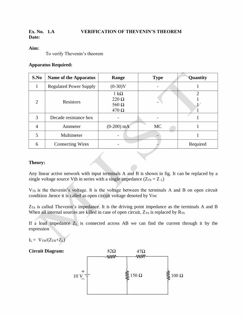
Circuit Diagram:
82Ω 47Ω
150 Ω 10 V 100 Ω
(0-20) V
MC V
82Ω 47Ω
150 Ω 10 V
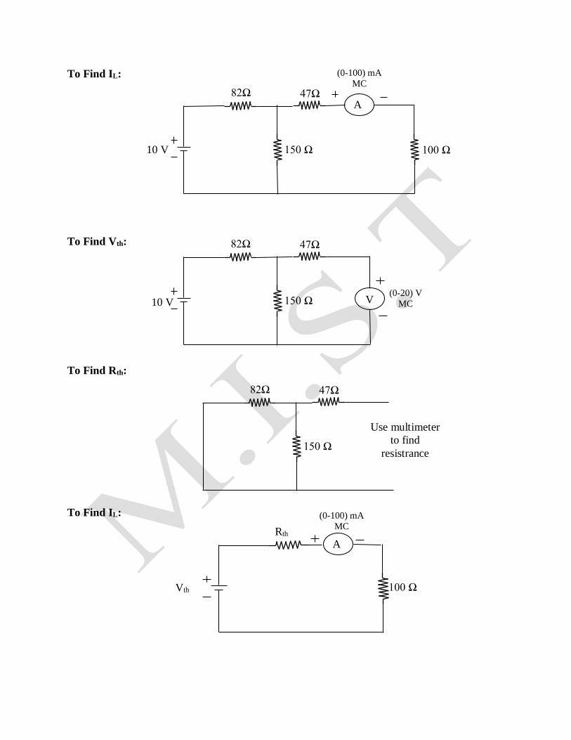
To Find IL:
To Find Vth:
To Find Rth:
To Find IL:
Rth
Vth
(0-100) mA
MC
A
100 Ω
82Ω 47Ω
150 Ω
Use multimeter
to find
resistrance
82Ω 47Ω
150 Ω 10 V 100 Ω
A
(0-100) mA
MC

Formulae used:
IL = Vth / (RL + Rth) in Amps.
Where IL = Load current in amps
Vth = Thevenin’s voltage in volts
RL = Load resistance in ohms
Rth = Thevenin’s resistance in ohms
Theoretical Calculation:
Tabulation:
Parameter
Theoretical Value
Practical Value
VTh
RTh
IL
Parameter
With Theorem
Without Theorem
IL

Procedure:
1. Give the connections as per the circuit diagram.
2. Set the required voltage by using RPS.
3. Replace load resistance by voltmeter for the same voltage.
4. Measure Voc(Vth) by using voltmeter for the same voltage.
5. Remove RPS from the circuit and short circuit the terminals to measure equivalent
resistance Rth.
6. Using thevenin’s equivalent circuit, the current through the load resistor IL is measured by
using an ammeter.
7. Verify thevenin’s theorem by comparing theoretical value and practical value.
Precaution:
1. Avoid loose connections.
2. Check the connections before giving supply.
3. Keep the RPS in Minimum Position.
Result:
Ex.No. 1.B VERIFICATION OF NORTON’S THEOREM
Date :
Aim:
To verify Norton’s theorem.
Apparatus Required:
S.No Name of the Apparatus Range Type Quantity
1 Regulated Power Supply (0-30)V - 1
2 Resistors
1 kΩ
220 Ω
560 Ω
470 Ω
-
2
1
1
1
3 Decade resistance box - - 1
4 Ammeter (0-200) mA MC 1
5 Multimeter - - 1
6 Connecting Wires - - Required
Theory:
Any linear active network with output terminals A and B is shown in fig. It can be
replaced by a single current source ISc = IN in parallel with a single impedance (RTh = R L). Isc is
the current through the terminals AB of the active network when shorted Zth is the thevenin’s
impedance. The current through impedance connected to the terminals of the Norton’s equivalent
circuit must have the same direction as the current through the same impedance connected to the
original active network. After evaluating the values of Isc and Rth.The current through Rl
connected across A and B we can find the current through it by the expression
IL = ( Isc x RN)/( RN +RL)
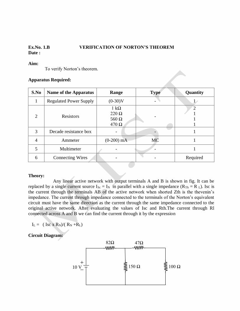
Circuit Diagram:
82Ω 47Ω
150 Ω 10 V 100 Ω
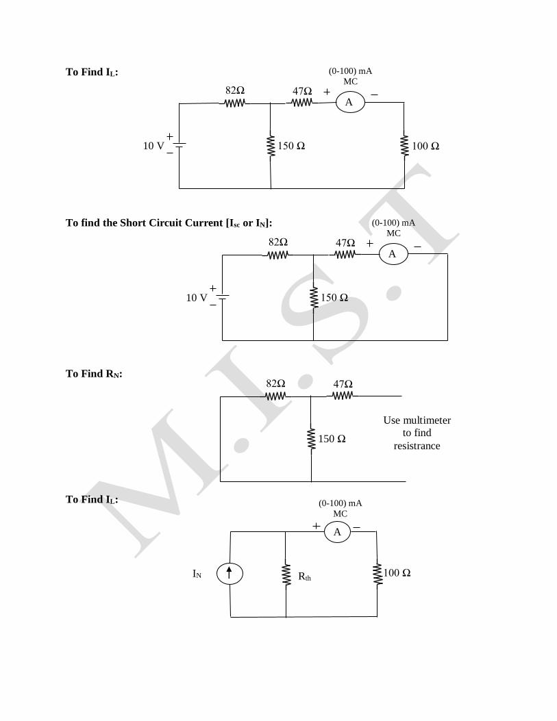
To Find IL:
To find the Short Circuit Current [Isc or IN]:
To Find RN:
To Find IL:
Rth IN
(0-100) mA
MC
100 Ω
A
82Ω 47Ω
150 Ω 10 V 100 Ω
A
(0-100) mA
MC
82Ω 47Ω
150 Ω 10 V
A
(0-100) mA
MC
82Ω 47Ω
150 Ω
Use multimeter
to find
resistrance

Formulae used:
To find IL:
By using current divider rule,
IL = (IN *RN)/( RN + RL)
Where,
IL = Load current in amps
IN = Norton’s current (or) Short circuit current in amps
RN = Norton’s resistance (or) Equivalent resistance in ohms
RL = Load resistance in ohms
Precaution:
1. Avoid loose connections.
2. Check the connections before giving supply.
3. Keep the RPS in Minimum Position.
Procedure:
1. Give the connections as per the circuit diagram
2. Set the required voltage by using RPS
3. The load resistance RL is removed and it is shorted to create a short circuit path and
measure the short circuit current using ammeter.
4. Remove RPS from the circuit and short circuit the terminals and measure the equivalent
resistance of the circuit RN.
5. Using Norton’s equivalent circuit, the current through the load and voltage across the load
is measured by using ammeter and voltmeter.
6. Verify Norton’s theorem by comparing theoretical value and practical value

Tabulation:
Theoretical Calculation:
Result:
Parameter
Theoretical Value
Practical Value
IN
RTh
IL
Parameter
With Theorem
With out Theorem
IL
Ex.No. 2.A VERIFICATION OF SUPERPOSITION AND RECIPROCITY
THEOREMS
Date :
Aim:
To verify superposition theorem.
Apparatus Required:
S.No Name of the Apparatus Range Type Quantity
1 Regulated Power Supply (0-30)V - 1
2 Resistors
1 kΩ
220 Ω
560 Ω
470 Ω
-
2
1
1
1
3 Ammeter (0-200) mA MC 1
4 Connecting Wires - - Required
Superposition Theorem:
Theory:
With the help of this theorem, we can find the current through or the voltage across a given
element in a linear circuit consisting of two or more sources. The statement is as follows:
In a linear circuit containing more than one source, the current that flows at any point or the
voltage that exists between any two points is the algebraic sum of the currents or the voltages that
would have been produced by each source taken separately with all other sources removed.
Circuit Diagram:
To find I:
82Ω 100Ω
56 Ω
15 V
A
10 V
(0-100) mA
MC
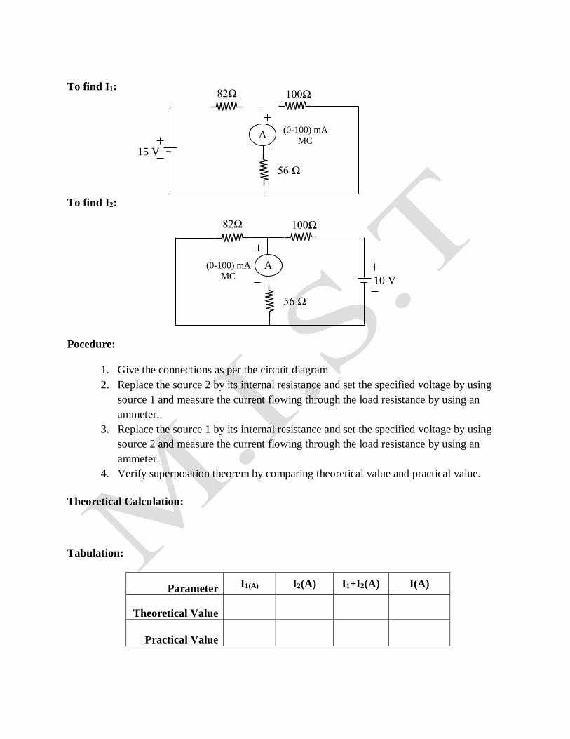
To find I1:
To find I2:
Pocedure:
1. Give the connections as per the circuit diagram
2. Replace the source 2 by its internal resistance and set the specified voltage by using
source 1 and measure the current flowing through the load resistance by using an
ammeter.
3. Replace the source 1 by its internal resistance and set the specified voltage by using
source 2 and measure the current flowing through the load resistance by using an
ammeter.
4. Verify superposition theorem by comparing theoretical value and practical value.
Theoretical Calculation:
Tabulation:
Parameter I1(A) I2(A) I1+I2(A) I(A)
Theoretical Value
Practical Value
82Ω 100Ω
56 Ω
A
10 V
(0-100) mA
MC
(0-100) mA
MC
82Ω 100Ω
56 Ω
15 V
A
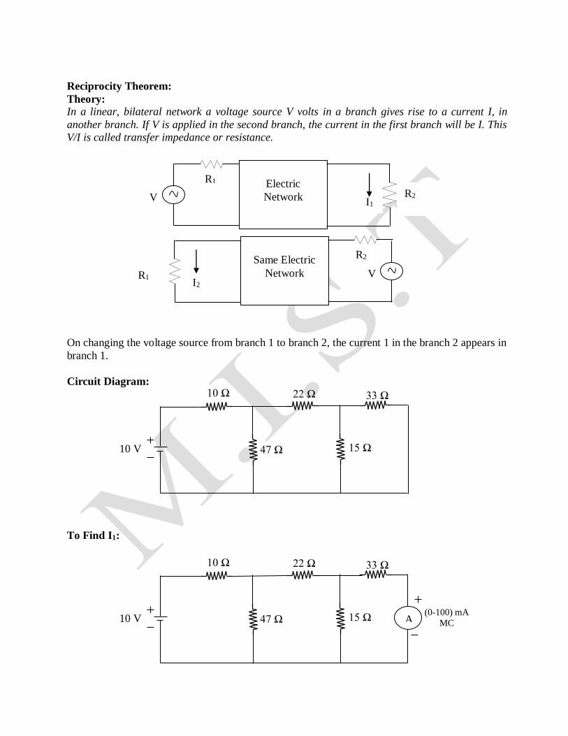
Reciprocity Theorem:
Theory: In a linear, bilateral network a voltage source V volts in a branch gives rise to a current I, in
another branch. If V is applied in the second branch, the current in the first branch will be I. This
V/I is called transfer impedance or resistance.
On changing the voltage source from branch 1 to branch 2, the current 1 in the branch 2 appears in
branch 1.
Circuit Diagram:
To Find I1:
Same Electric
Network R1
R2
I2
Electric
Network V
R1
R2 I1
V
10 Ω
47 Ω 10 V
22 Ω 33 Ω
15 Ω
10 Ω
47 Ω 10 V
22 Ω 33 Ω
15 Ω A (0-100) mA
MC
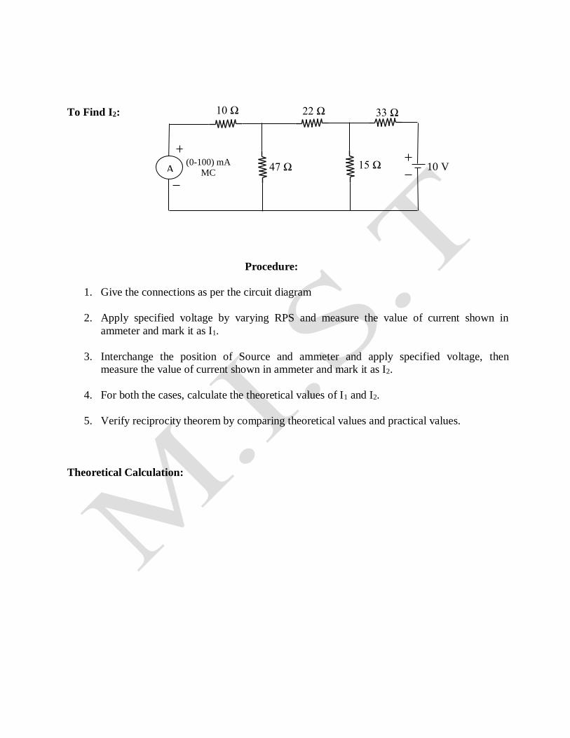
To Find I2:
Procedure:
1. Give the connections as per the circuit diagram
2. Apply specified voltage by varying RPS and measure the value of current shown in
ammeter and mark it as I1.
3. Interchange the position of Source and ammeter and apply specified voltage, then
measure the value of current shown in ammeter and mark it as I2.
4. For both the cases, calculate the theoretical values of I1 and I2.
5. Verify reciprocity theorem by comparing theoretical values and practical values.
Theoretical Calculation:
10 Ω
47 Ω 10 V
22 Ω 33 Ω
15 Ω A (0-100) mA
MC

Tabulation:
Precaution:
1. Avoid loose connections.
2. Check the connections before giving supply.
3. Keep the RPS in Minimum Position.
Result:
Parameter
Theoretical Value
Practical Value
I1
I2
MAXIMUM POWER TRANSFER THEOREM Exp. No. 2.B
Date:
AIM:- To verify the maximum power transfer theorem.
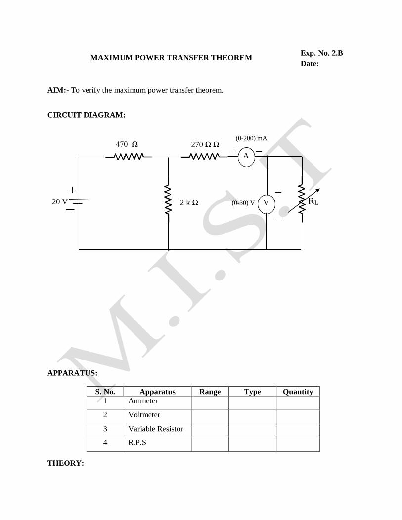
CIRCUIT DIAGRAM:
APPARATUS:
S. No. Apparatus Range Type Quantity
1 Ammeter
2 Voltmeter
3 Variable Resistor
4 R.P.S
THEORY:
270 Ω Ω 470 Ω
2 k Ω RL 20 V
A
V (0-30) V
(0-200) mA

DC Circuit: The maximum power transfer theorem states that “maximum power is delivered from a source
resistance to a load resistance when the load resistance is equal to source resistance.”
Rs = RL is the condition required for maximum power transfer.
PROCEDURE:
1. Connect the circuit as per the practical circuit shown in fig.1
2. Vary the load resistance in steps and note down voltage across the load and current
flowing through the circuit.
3. Calculate power delivered to the load by using formula P=V X l
4. Draw the graph between resistance and power (resistance on X- axis and power on Y-
axis).
5. Verify the maximum power is delivered to the load when RL = Rs.
TABULAR COLUMN:
R VL IL P=VLIL
THEORETICAL CALCULATIONS: Maximum Power = PMax = VTH
2 / 4RL
Parameters Theoretical Value (PMax) Practical Value (PMax)
D.C. Circuit
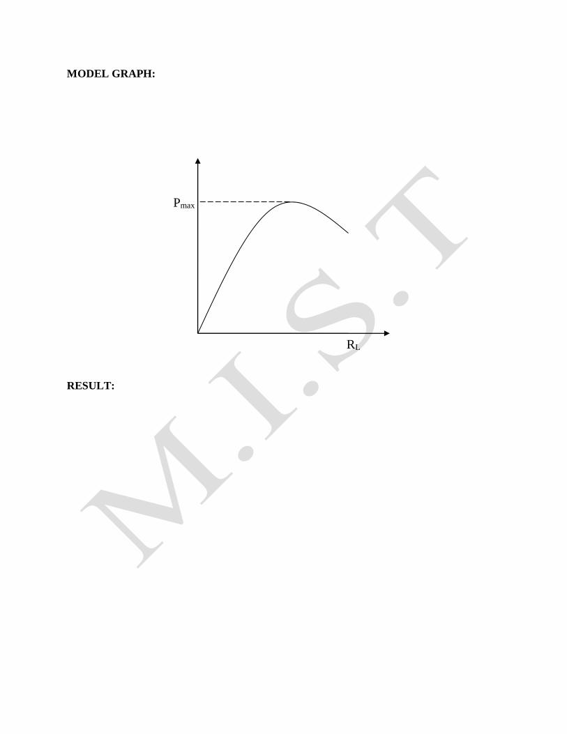
MODEL GRAPH:
RESULT:
Pmax
RL
EXP: 3
LOCUS DIAGRAMS OF RL AND RC SERIES CICUITS.
AIM:-To draw the current locus of RL and RC circuits with L & C variables
respectively.
APPARATUS:-
S.No Name of the equipment Range Type Quantity
1.
2.
3.
4.
5.
6.
7.
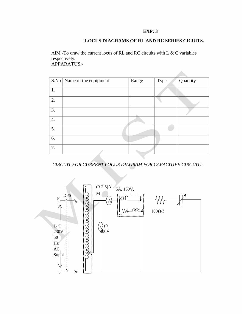
CIRCUIT FOR CURRENT LOCUS DIAGRAM FOR CAPACITIVE CIRCUIT:-
(0-2.5)A 5A, 150V,
UPF P
DPST
MI
A M L
V 100Ω/5A C
1- Φ
230V
50
Hz
AC
Suppl
y
V (0-
300V MI)
(0-2.5)A 5A,
150V,UPF P
DPST
MI
A M L
V 100Ω/5A C
1- Φ
230V
50
Hz
AC
Suppl
y
V (0-
300V MI)
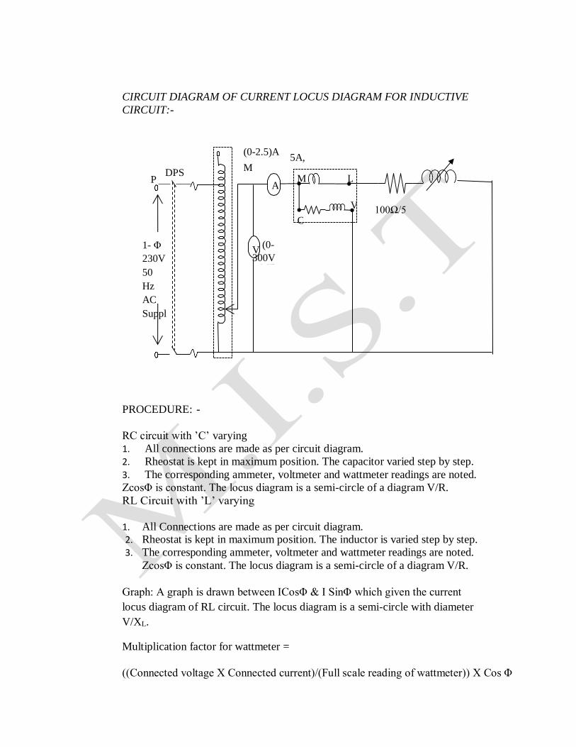
CIRCUIT DIAGRAM OF CURRENT LOCUS DIAGRAM FOR INDUCTIVE
CIRCUIT:-
PROCEDURE: -
RC circuit with ’C’ varying
1. All connections are made as per circuit diagram.
2. Rheostat is kept in maximum position. The capacitor varied step by step.
3. The corresponding ammeter, voltmeter and wattmeter readings are noted.
ZcosΦ is constant. The locus diagram is a semi-circle of a diagram V/R.
RL Circuit with ’L’ varying
1. All Connections are made as per circuit diagram. 2. Rheostat is kept in maximum position. The inductor is varied step by step.
3. The corresponding ammeter, voltmeter and wattmeter readings are noted.
ZcosΦ is constant. The locus diagram is a semi-circle of a diagram V/R.
Graph: A graph is drawn between ICosΦ & I SinΦ which given the current
locus diagram of RL circuit. The locus diagram is a semi-circle with diameter
V/XL.
Multiplication factor for wattmeter =
((Connected voltage X Connected current)/(Full scale reading of wattmeter)) X Cos Φ

Observations:
RL Circuits with L as variable:-
S.N
o
V I W Z=V/I CosΦ=W/V
I
sin
Φ
Zc
os
Φ
I
Co
sΦ
I SinΦ
RC Circuits with C as variable:-
S.N
o
V I W Z=V/I CosΦ=W/
VI
sinΦ ZcosΦ I
CosΦ
I SinΦ
RESULT:-
SERIES AND PARALLEL RESONANCE Exp. No. 4
Date:
AIM:
To find the resonant frequency, quality factor, and band width of a series and parallel
resonant circuit.
APPARATUS REQUIRED :
S. No. Apparatus Range Type Quantity
1 Function generator - - 1
2 Decade resistance box - - 1
3 Decade inductance box - - 1
4 Decade capacitance box - - 1
5 Ammeter (0-100)mA DC 1
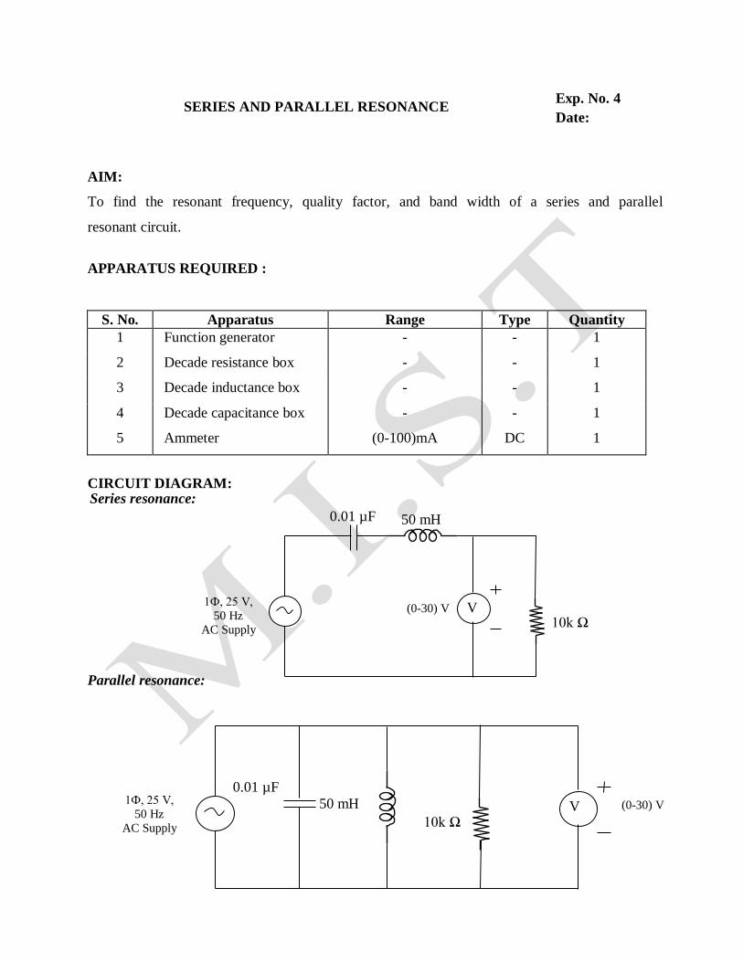
CIRCUIT DIAGRAM: Series resonance:
Parallel resonance:
10k Ω
1Ф, 25 V,
50 Hz
AC Supply
0.01 µF 50 mH
V (0-30) V
10k Ω
1Ф, 25 V,
50 Hz
AC Supply
0.01 µF
50 mH V (0-30) V
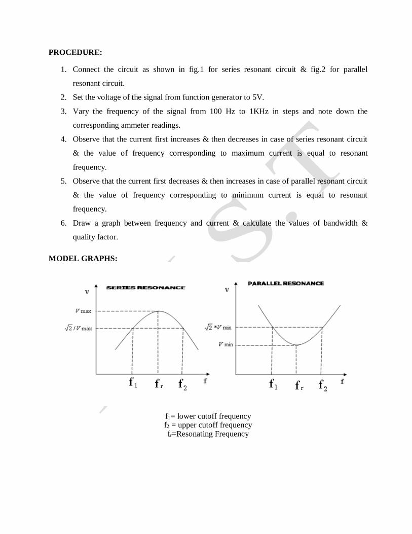
PROCEDURE:
1. Connect the circuit as shown in fig.1 for series resonant circuit & fig.2 for parallel
resonant circuit.
2. Set the voltage of the signal from function generator to 5V.
3. Vary the frequency of the signal from 100 Hz to 1KHz in steps and note down the
corresponding ammeter readings.
4. Observe that the current first increases & then decreases in case of series resonant circuit
& the value of frequency corresponding to maximum current is equal to resonant
frequency.
5. Observe that the current first decreases & then increases in case of parallel resonant circuit
& the value of frequency corresponding to minimum current is equal to resonant
frequency.
6. Draw a graph between frequency and current & calculate the values of bandwidth &
quality factor.
MODEL GRAPHS:
f1= lower cutoff frequency f2 = upper cutoff frequency fr=Resonating Frequency

TABULATION : Series Resonance
S. No. Frequency
(Hz)
Voltage
(V)
TABULATION : Parallel Resonance
S. No. Frequency
(Hz)
Voltage
(V)
RESULT:
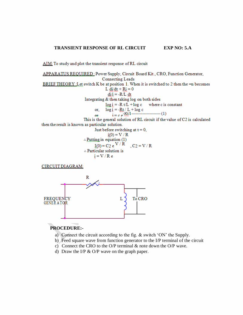
TRANSIENT RESPONSE OF RL CIRCUIT EXP NO: 5.A
PROCEDURE:-
a) Connect the circuit according to the fig. & switch ‘ON’ the Supply.
b) Feed square wave from function generator to the I/P terminal of the circuit
c) Connect the CRO to the O/P terminal & note down the O/P wave.
d) Draw the I/P & O/P wave on the graph paper.
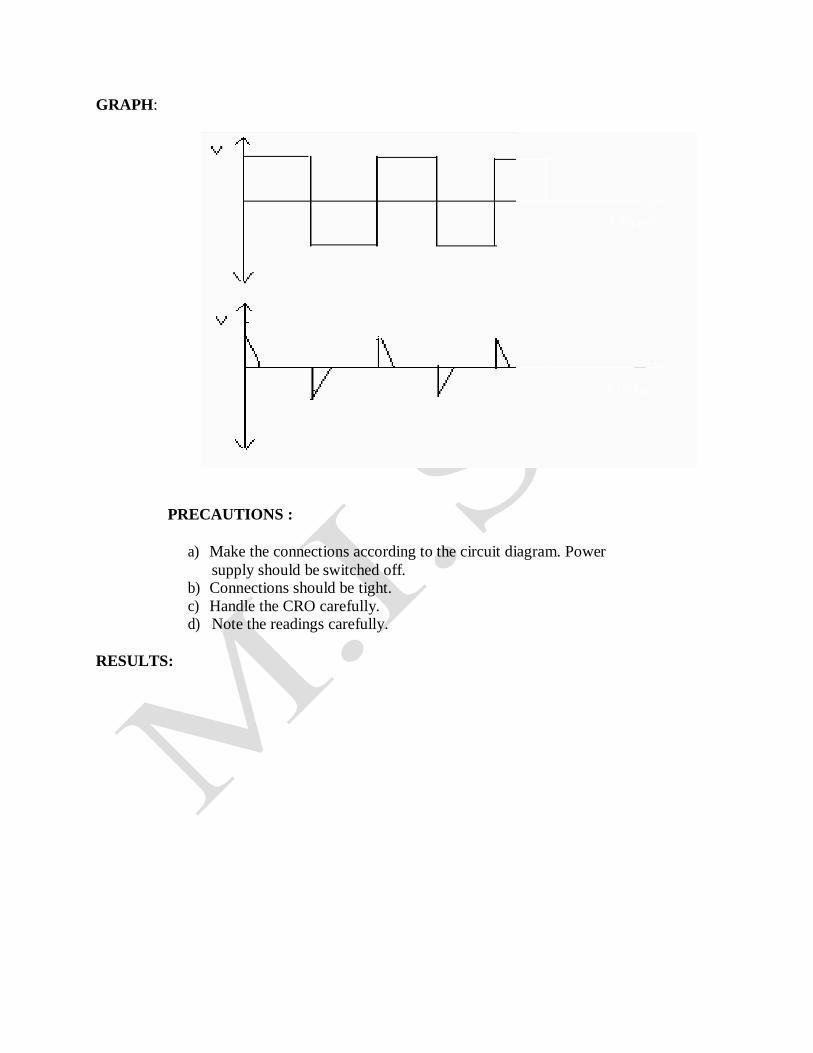
GRAPH:
PRECAUTIONS :
a) Make the connections according to the circuit diagram. Power
supply should be switched off. b) Connections should be tight.
c) Handle the CRO carefully. d) Note the readings carefully.
RESULTS:
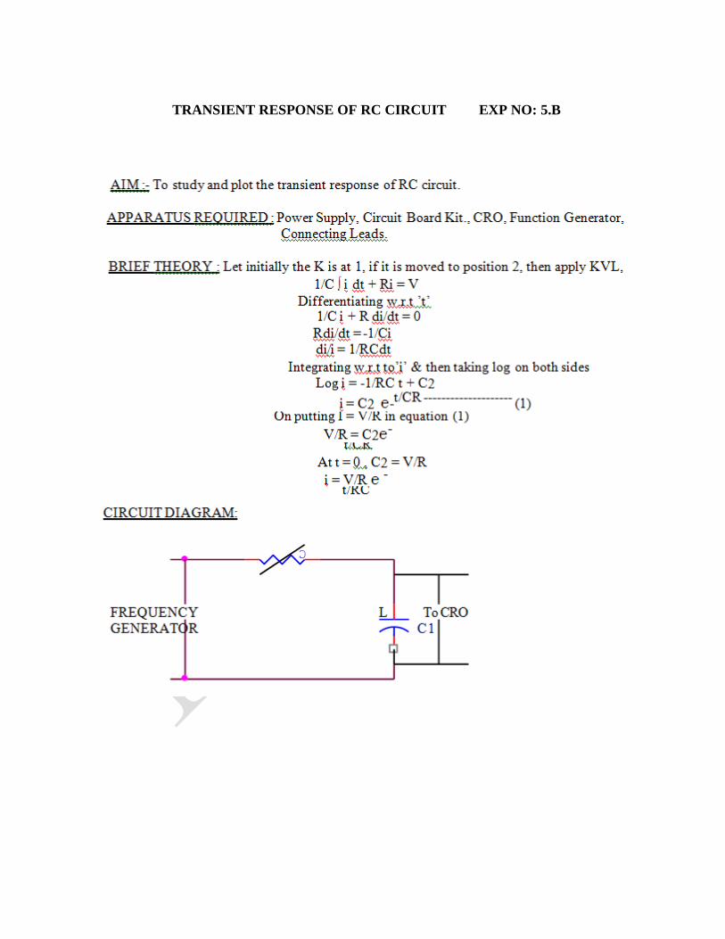
TRANSIENT RESPONSE OF RC CIRCUIT EXP NO: 5.B
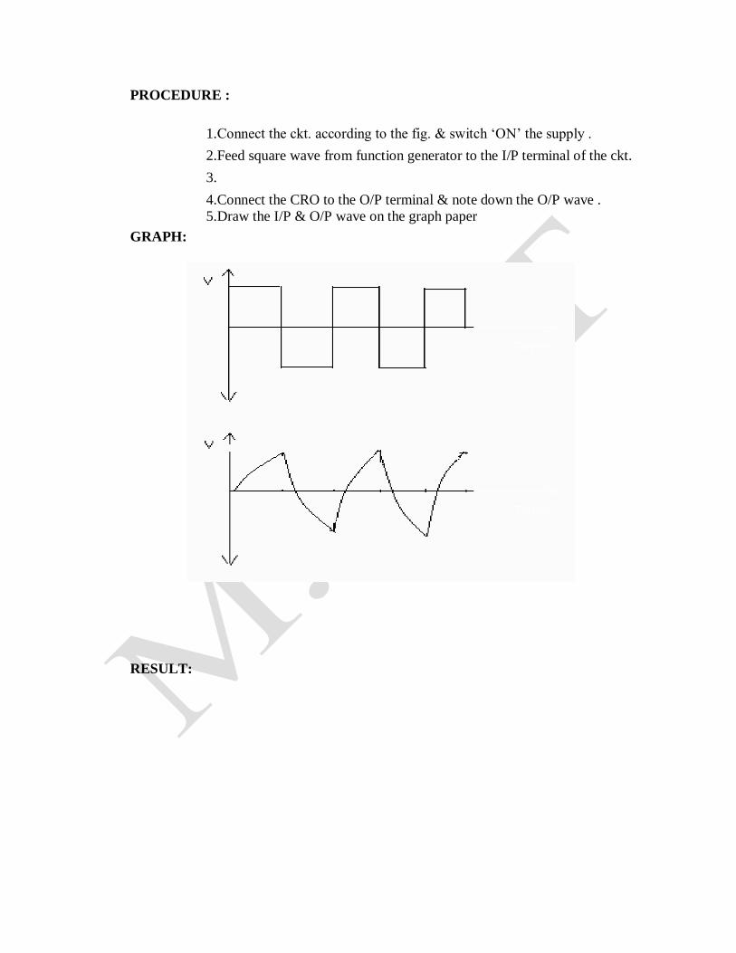
PROCEDURE :
1.Connect the ckt. according to the fig. & switch ‘ON’ the supply .
2.Feed square wave from function generator to the I/P terminal of the ckt.
3.
4.Connect the CRO to the O/P terminal & note down the O/P wave .
5.Draw the I/P & O/P wave on the graph paper
GRAPH:
RESULT:
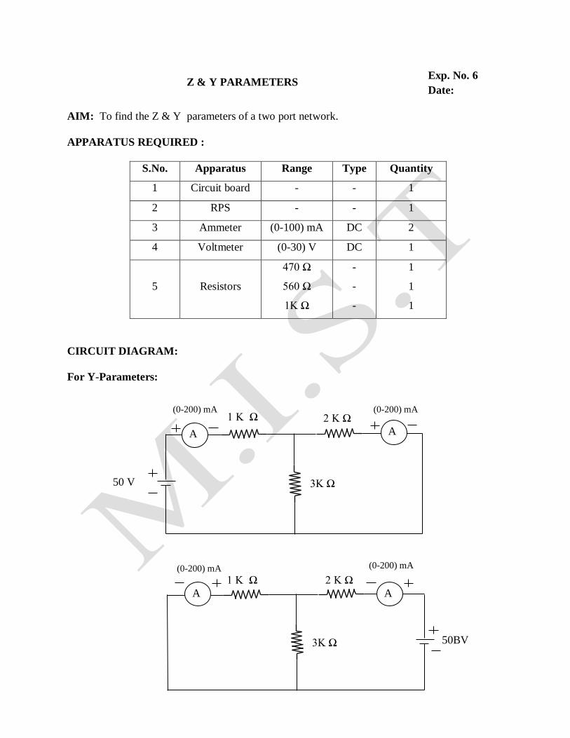
Z & Y PARAMETERS Exp. No. 6
Date:
AIM: To find the Z & Y parameters of a two port network.
APPARATUS REQUIRED :
S.No. Apparatus Range Type Quantity
1 Circuit board - - 1
2 RPS - - 1
3 Ammeter (0-100) mA DC 2
4 Voltmeter (0-30) V DC 1
5 Resistors
470 Ω
560 Ω
1K Ω
-
-
-
1
1
1
CIRCUIT DIAGRAM:
For Y-Parameters:
3K Ω
2 K Ω 1 K Ω
50BV
A A
(0-200) mA
(0-200) mA
3K Ω
2 K Ω 1 K Ω
50 V
(0-200) mA
(0-200) mA
A A
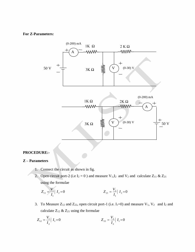
For Z-Parameters:
PROCEDURE:-
Z – Parameters
1. Connect the circuit as shown in fig.
2. Open circuit port-2 (i.e I2 = 0 ) and measure V1,I2 and V2 and calculate Z11 & Z21
using the formulae
02
1
111 I
I
VZ 02
1
221 I
I
VZ
3. To Measure Z12 and Z22, open circuit port-1 (i.e. I1=0) and measure V1, V2 and I2 and
calculate Z12 & Z21 using the formulae
01
2
112 I
I
VZ 01
2
222 I
I
VZ
3K Ω
2 K Ω 1K Ω
50 V (0-30) V
(0-200) mA
A
V
3K Ω
2K Ω 1K Ω
50 V (0-30) V
(0-200) mA
V
A
Y – Parameters
1. Connect the circuit as shown in fig.
2. Short circuit port-2 (i.e V2 = 0 ) and measure V1, I1 & I2 and
calculate Y11 & Y21 using the formulae
02
1
111 V
V
IY 02
1
221 V
V
IY
3. To Measure Y12 and Y22, short circuit port-1 (i.e. V1=0) and measure V2, I1 and I2 and
calculate Y12 & Y22 using the formulae
01
2
112 V
V
IY 01
2
222 V
V
IY
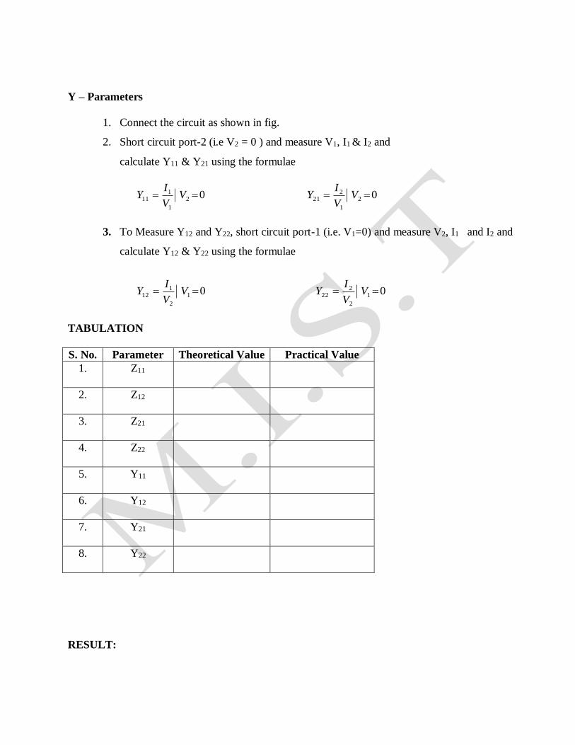
TABULATION
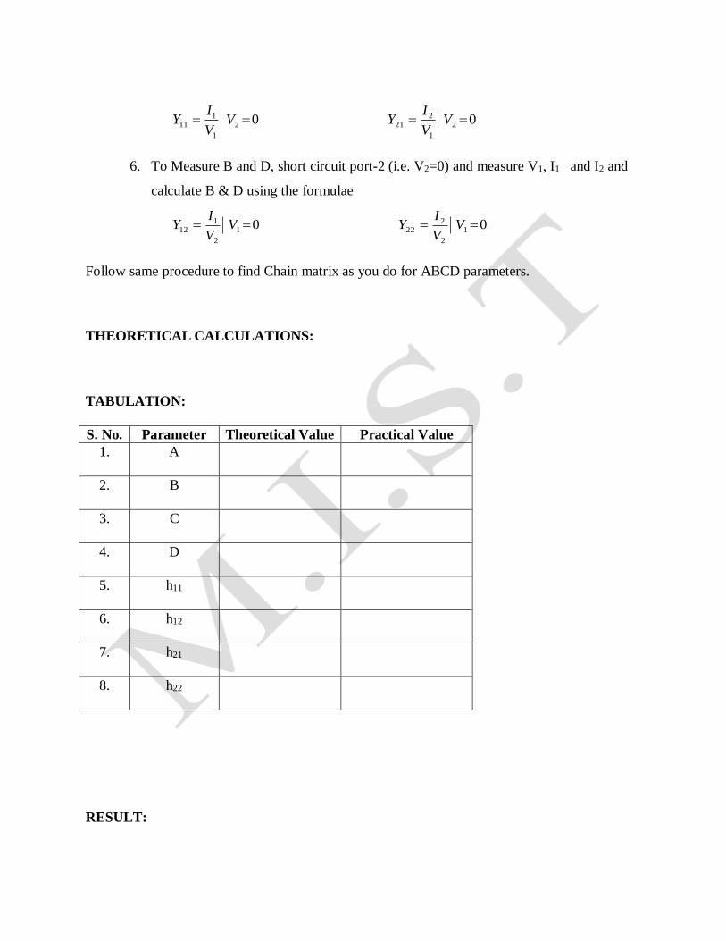
S. No. Parameter Theoretical Value Practical Value
1. Z11
2. Z12
3. Z21
4. Z22
5. Y11
6. Y12
7. Y21
8. Y22
RESULT:
H, ABCD PARAMETERS & CHAIN MATRIX Exp. No. 7
Date:
AIM: To find the H, ABCD and to verify CHAIM MATRIX of a two port network.
APPARATUS REQUIRED :
S.No. Apparatus Range Type Quantity
1 Circuit board - - 1
2 RPS - - 1
3 Ammeter (0-100) mA DC 2
4 Voltmeter (0-30) V DC 1
5 Resistors
470 Ω
560 Ω
1K Ω
-
-
-
2
2
2
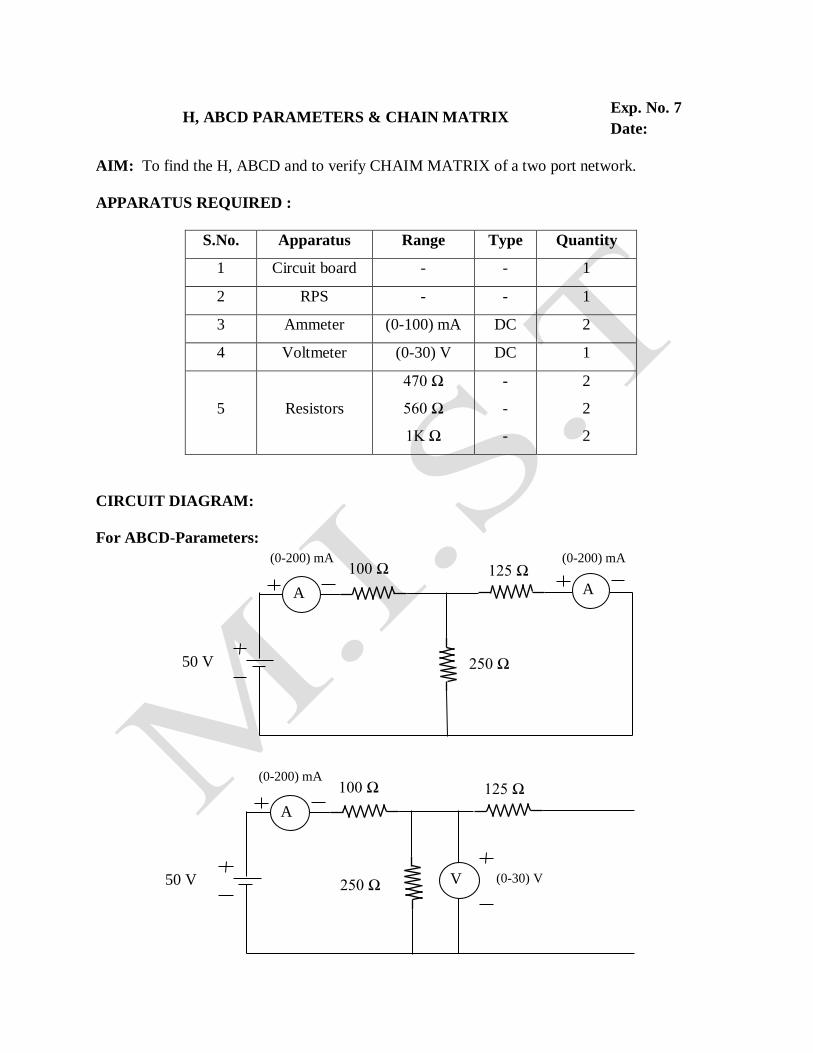
CIRCUIT DIAGRAM:
For ABCD-Parameters:
250 Ω
125 Ω 100 Ω
50 V
(0-200) mA
(0-200) mA
A A
250 Ω
125 Ω 100 Ω
50 V (0-30) V
(0-200) mA
A
V
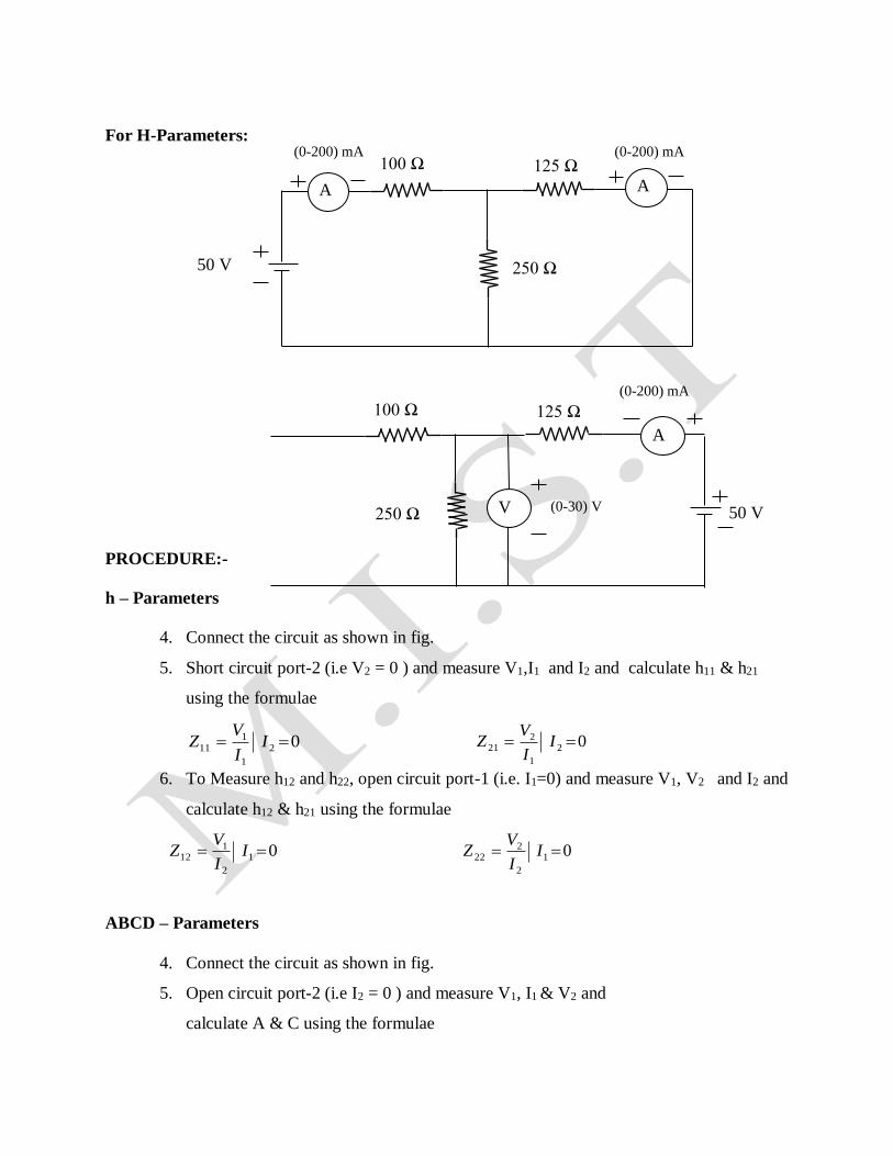
For H-Parameters:
PROCEDURE:-
h – Parameters
4. Connect the circuit as shown in fig.
5. Short circuit port-2 (i.e V2 = 0 ) and measure V1,I1 and I2 and calculate h11 & h21
using the formulae
02
1
111 I
I
VZ 02
1
221 I
I
VZ
6. To Measure h12 and h22, open circuit port-1 (i.e. I1=0) and measure V1, V2 and I2 and
calculate h12 & h21 using the formulae
01
2
112 I
I
VZ 01
2
222 I
I
VZ
ABCD – Parameters
4. Connect the circuit as shown in fig.
5. Open circuit port-2 (i.e I2 = 0 ) and measure V1, I1 & V2 and
calculate A & C using the formulae
250 Ω
125 Ω 100 Ω
50 V
(0-200) mA
(0-200) mA
A A
250 Ω
125 Ω 100 Ω
50 V (0-30) V
(0-200) mA
V
A
02
1
111 V
V
IY 02
1
221 V
V
IY
6. To Measure B and D, short circuit port-2 (i.e. V2=0) and measure V1, I1 and I2 and
calculate B & D using the formulae
01
2
112 V
V
IY 01
2
222 V
V
IY
Follow same procedure to find Chain matrix as you do for ABCD parameters.
THEORETICAL CALCULATIONS:
TABULATION:
S. No. Parameter Theoretical Value Practical Value
1. A
2. B
3. C
4. D
5. h11
6. h12
7. h21
8. h22
RESULT:
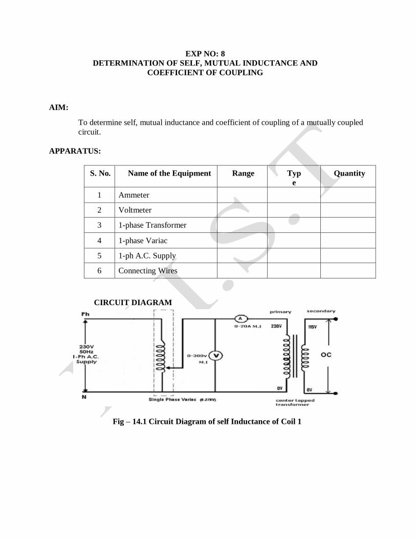
EXP NO: 8
DETERMINATION OF SELF, MUTUAL INDUCTANCE AND
COEFFICIENT OF COUPLING
AIM:
To determine self, mutual inductance and coefficient of coupling of a mutually coupled
circuit.
APPARATUS:
S. No. Name of the Equipment Range Typ
e
Quantity
1 Ammeter
2 Voltmeter
3 1-phase Transformer
4 1-phase Variac
5 1-ph A.C. Supply
6 Connecting Wires
CIRCUIT DIAGRAM
Fig – 14.1 Circuit Diagram of self Inductance of Coil 1
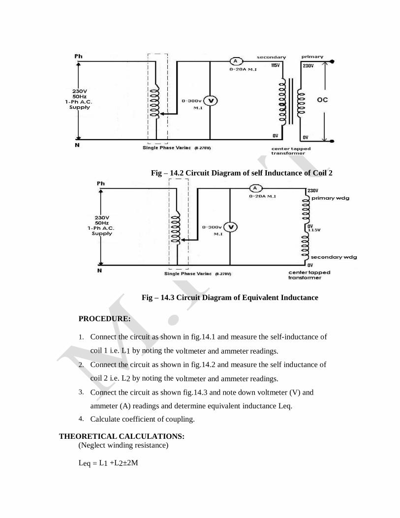
Fig – 14.2 Circuit Diagram of self Inductance of Coil 2
Fig – 14.3 Circuit Diagram of Equivalent Inductance
PROCEDURE:
1. Connect the circuit as shown in fig.14.1 and measure the self-inductance of
coil 1 i.e. L1 by noting the voltmeter and ammeter readings.
2. Connect the circuit as shown in fig.14.2 and measure the self inductance of
coil 2 i.e. L2 by noting the voltmeter and ammeter readings.
3. Connect the circuit as shown fig.14.3 and note down voltmeter (V) and
ammeter (A) readings and determine equivalent inductance Leq.
4. Calculate coefficient of coupling.
THEORETICAL CALCULATIONS:
(Neglect winding resistance)
Leq = L1 +L2±2M
Mutual Inductance M=[(Leq – (L1+L2))/2]
Coefficient of Coupling K = M/√ (L1L2)
Where L1 and L2 are determined as follows
Determination of L1
From fig.14.1
XL1= voltmeter reading /ammeter reading
XL1= ωL1 = 2ΠfL1
L1 = XL1/2Πf (Henry)
Determination of L2
From fig 14.2
XL2 = Voltmeter reading /Ammeter reading
XL2 = ωL2 = 2ΠfL2
L2= XL2/2Πf (Henry)
Determination of Leq
From fig 14.3
XLeq = Voltmeter reading /Ammeter reading
XLeq = ωLeq = 2ΠfLeq
Leq = XLeq/2Πf (Henry)
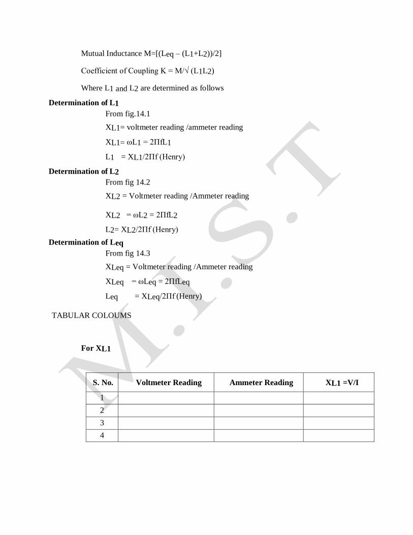
TABULAR COLOUMS
For XL1
S. No. Voltmeter Reading Ammeter Reading XL1 =V/I
1
2
3
4
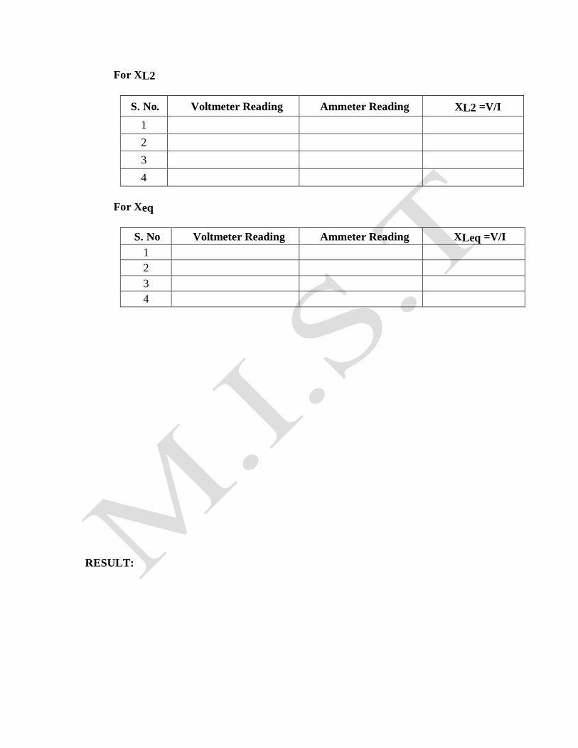
For XL2
S. No. Voltmeter Reading Ammeter Reading XL2 =V/I
1
2
3
4
For Xeq
S. No Voltmeter Reading Ammeter Reading XLeq =V/I
1
2
3
4
RESULT:
EXP NO:9.A
VERIFICATION OF COMPENSATION THEOREM
AIM:
To verify the compensation theorem and to determine the change in current.
APPARATUS:
S. No. Name of the
Equipment
Range Type Quantity
1 Ammeter
2 Voltmeter
3 R.P.S
4 Resistors
5 Bread Board
6 Connecting Wires
STATEMENT
Compensation theorem states that any element in electrical network can be
replaced by its equivalent voltage source, whose value is equal to product of
current flowing through it and its value. (Compensation theorem got the
importance of determining the change in current flowing through element or
circuit because of change in the resistance value).
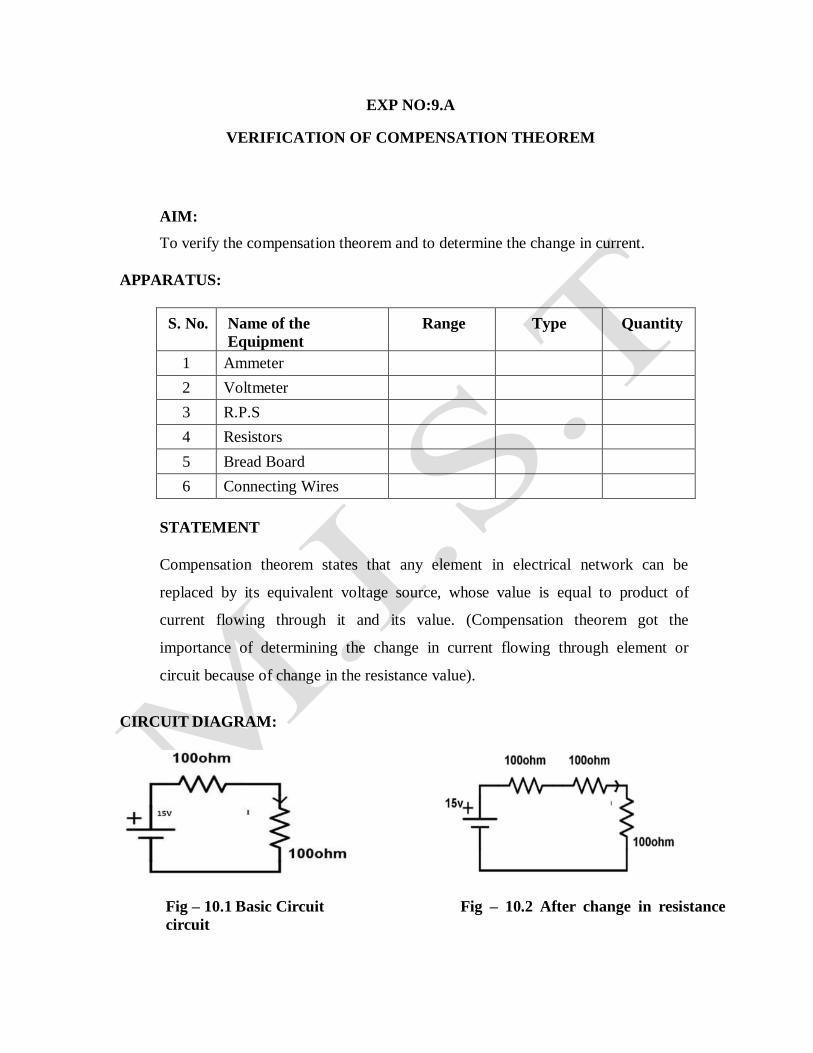
CIRCUIT DIAGRAM:
Fig – 10.1 Basic Circuit Fig – 10.2 After change in resistance
circuit

Fig -10.3 Compensation Theorem Circuit
PROCEDURE:
1. Connect the circuit as shown in fig10.1.
2. Measure the current I..
3. Connect the circuit as shown in fig10.2. by increasing the
circuit resistance(∆R), Measure the current I1.
4. The change in current in the circuit can be found by connecting a voltage
source equal to I1∆R as shown in fig10.3.
5. Measure the current I" i.e., the change in current.
6. Observe that I"= I- I1.
TABULAR COLUMN:
S.No
.
Parameters
Theoretical value
Practical value
1
2
3
RESULT:
EXP NO:9.B
VERIFICATION OF MILLIMAN'S THEOREM
AIM:
To verify the Milliman’s Theorem.
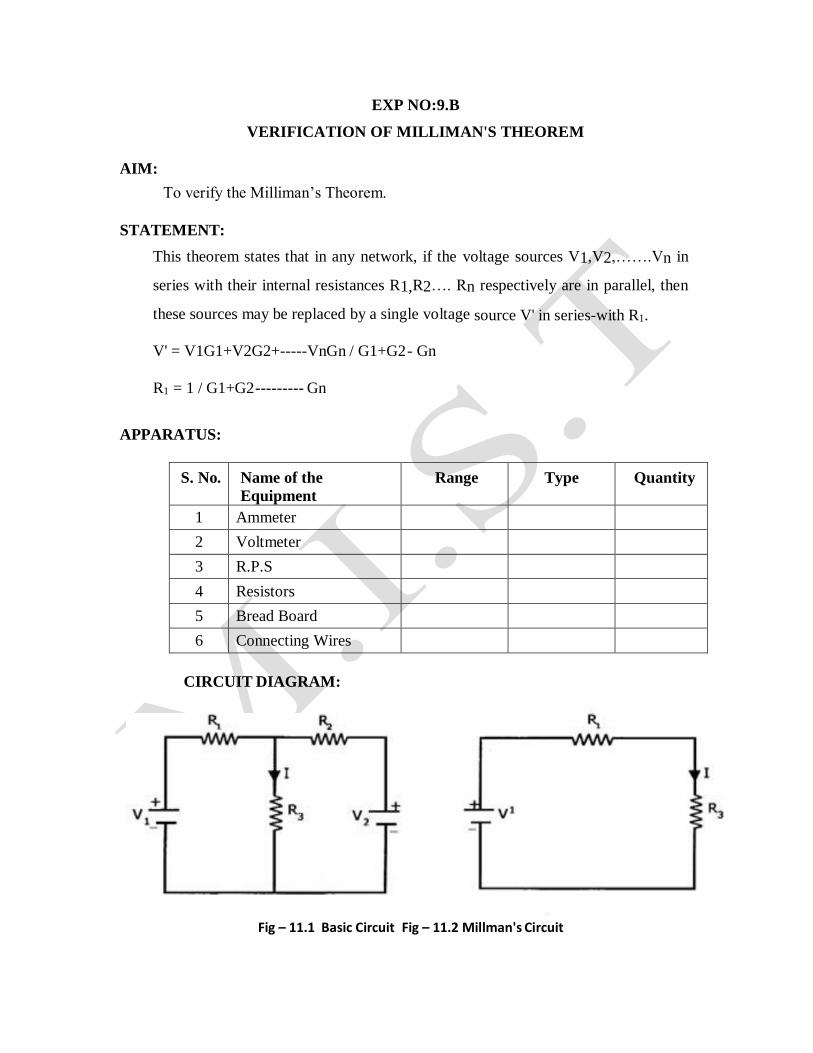
STATEMENT:
This theorem states that in any network, if the voltage sources V1,V2,…….Vn in
series with their internal resistances R1,R2…. Rn respectively are in parallel, then
these sources may be replaced by a single voltage source V' in series-with R1.
V' = V1G1+V2G2+-----VnGn / G1+G2 - Gn
R1 = 1 / G1+G2 --------- Gn
APPARATUS:
S. No. Name of the
Equipment
Range Type Quantity
1 Ammeter
2 Voltmeter
3 R.P.S
4 Resistors
5 Bread Board
6 Connecting Wires
CIRCUIT DIAGRAM:
Fig – 11.1 Basic Circuit Fig – 11.2 Millman's Circuit
PROCEDURE:
1. Connect the circuit as shown in fig.11.1
2. Measure the current through the resistor R3.
3. Connect the circuit as shown in fig.11.2 and measure the current through R3.
4. Observe that the two currents are same.
TABULAR COLUMN:
S.No. Parameters Theoretical value Practical value
1
2
RESULT:
EXP NO:10
AVERAGE VALUE, RMS VALUE, FORM FACTOR, PEAK
FACTOR OF SINUSOIDAL WAVE, SQUARE WAVE
AIM:
To determine the average value, RMS value, form factor, peak factor of
sinusoidal wave, square wave.
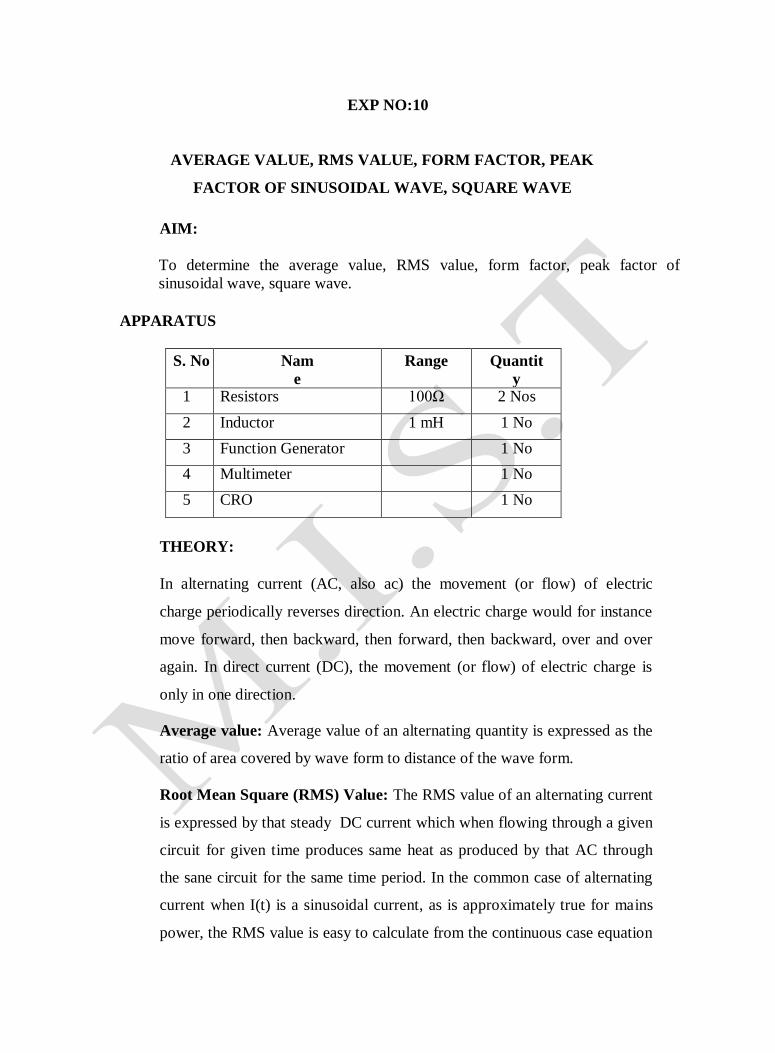
APPARATUS
S. No Nam
e
Range Quantit
y 1 Resistors 100Ω 2 Nos
2 Inductor 1 mH 1 No
3 Function Generator 1 No
4 Multimeter 1 No
5 CRO 1 No
THEORY:
In alternating current (AC, also ac) the movement (or flow) of electric
charge periodically reverses direction. An electric charge would for instance
move forward, then backward, then forward, then backward, over and over
again. In direct current (DC), the movement (or flow) of electric charge is
only in one direction.
Average value: Average value of an alternating quantity is expressed as the
ratio of area covered by wave form to distance of the wave form.
Root Mean Square (RMS) Value: The RMS value of an alternating current
is expressed by that steady DC current which when flowing through a given
circuit for given time produces same heat as produced by that AC through
the sane circuit for the same time period. In the common case of alternating
current when I(t) is a sinusoidal current, as is approximately true for mains
power, the RMS value is easy to calculate from the continuous case equation
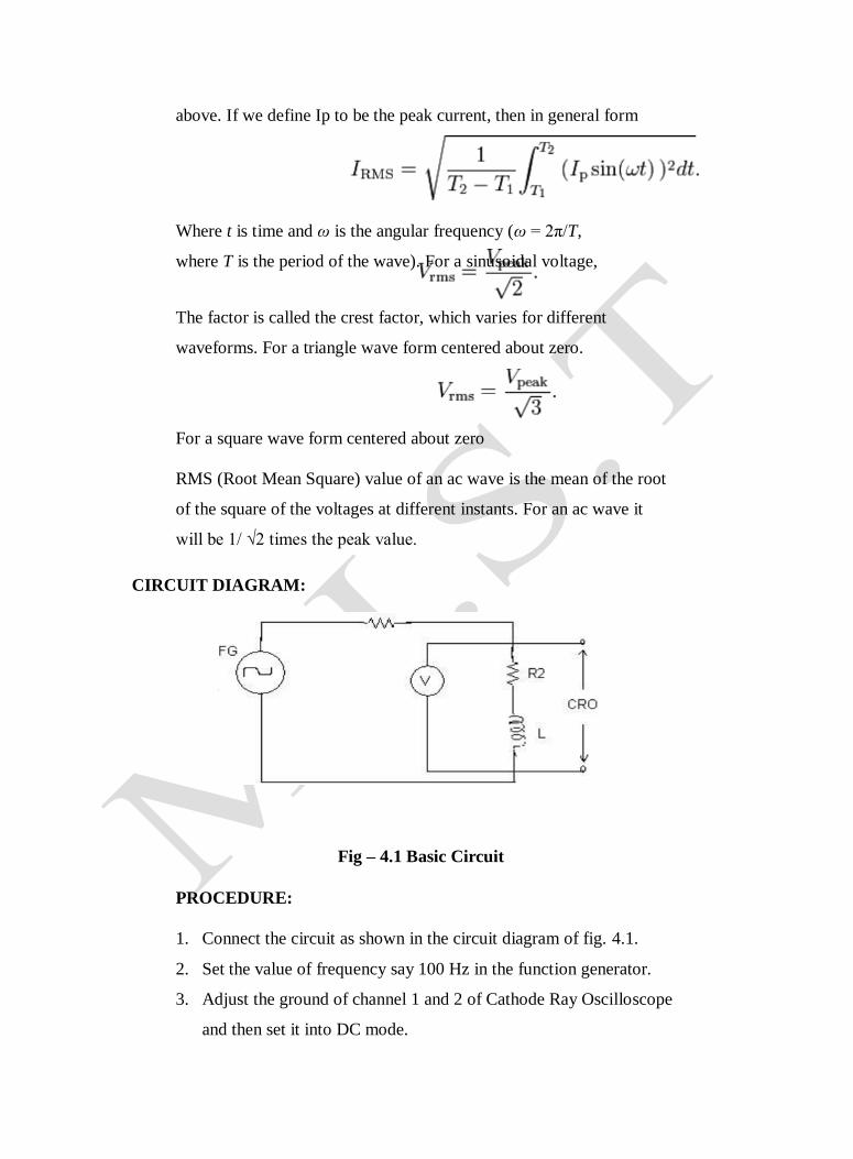
above. If we define Ip to be the peak current, then in general form
Where t is time and ω is the angular frequency (ω = 2π/T,
where T is the period of the wave). For a sinusoidal voltage,
The factor is called the crest factor, which varies for different
waveforms. For a triangle wave form centered about zero.
For a square wave form centered about zero
RMS (Root Mean Square) value of an ac wave is the mean of the root
of the square of the voltages at different instants. For an ac wave it
will be 1/ √2 times the peak value.
CIRCUIT DIAGRAM:
Fig – 4.1 Basic Circuit
PROCEDURE:
1. Connect the circuit as shown in the circuit diagram of fig. 4.1.
2. Set the value of frequency say 100 Hz in the function generator.
3. Adjust the ground of channel 1 and 2 of Cathode Ray Oscilloscope
and then set it into DC mode.
4. Connect CRO across the load in DC mode and observe the waveform.
Adjust the DC offset of function generator.
5. Note down the amplitude and frequency.
6. Set the multimeter into AC mode and measure input voltage and voltage
across point AB. This value gives RMS value of sinusoidal AC.
7. Calculate the average value.
8. Repeat experiment for different frequency and different peak to peak voltage.
Measure the RMS and Average value of DC signal also where
instead of function generator you can use DC supply.
OBSERVATIONS & CALCULATIONS:
Peak value
(V)
RMS value
(V)
Average value
(V)
PRECAUTIONS:
1. Check for proper connections before switching ON the supply
2. Make sure of proper color coding of resistors
3. The terminal of the resistance should be properly connected
RESULT:
EXP NO: 11
MEASUREMENT OF REACTIVE POWER FOR STAR AND DELTA
CONNECTED NETWORK
Aim: To measure the active power for the given star and delta network.
Apparatus:
S.No Name of the equipment Range Type Quantity
1 Wattmeter 0-10A/600V UPF 2
2 3- Φ Reactive load 10A Wire wound 1
3 Connecting wires - - As per the
requirement
Theory:
A three phase balanced voltage is applied on a balanced three phase load when the current
in each of the phase lags by an angle Φ behind corresponding phase voltages. Current
through current coil of w1=Ir, current through current coil of W2=IB, while potential
difference across voltage coil of W1=VRN-VYN=VRY(line voltage), and the potential
difference across voltage coil of W2= VRN-VYN=VBY.
Also , phase difference between IR and VRY is (300+ Φ).While that between IB and VBY is
(300- Φ). Thus reading on wattmeter W1 is given by W1=VRYIYCos(300+ Φ) While reading
on wattmeter W2 is given by W2=VBYIBCos(300- Φ) Since the load is balanced,
|IR|=|IY|=|IB|=I and |VRY|=|VBY|=VL
Thus total power P is given by
W= W1 +W2 = VLICos(300+ Φ) + VLICos(300- Φ)
= VLI[Cos(300+ Φ) + Cos(300- Φ)]
= [√3/2 *2Cos Φ]VLI
= √3VLICos Φ.
Reactive Power=√3(W1 -W2)
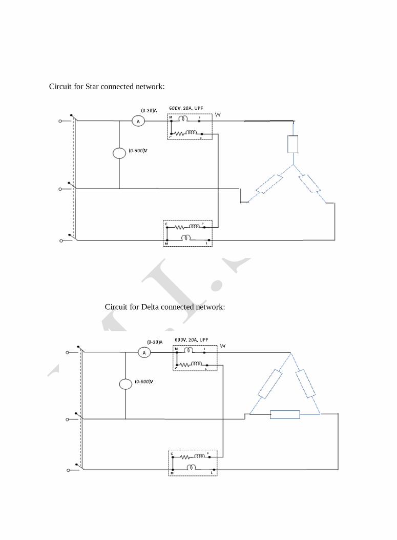
Circuit for Star connected network:
Circuit for Delta connected network:

Procedure:
(Star connection):
1) Connect the circuit as shown in the figure.
2) Ammeter is connected in series with wattmeter whose other
end is connected to one of the loads of the balanced loads.
3) The Y-phase is directly connected to one of the nodes of the 3-ph
supply.
4) A wattmeter is connected across R-phase & Y-phase as shown
in fig. The extreme of B- phase is connected to the third
terminal of the balanced 3-ph load.
5) Another wattmeter is connected across Y & B phase, the
extreme of B-phase is connected to the third terminal of the
balanced three phases load.
6) Verify the connections before switching on the 3-ph power supply.
(Delta connection):
1) Connect the circuit as shown in the figure.
2) Ammeter is connected in series with wattmeter whose other
end is connected to one of the loads of the balanced loads.
3) The Y-phase is directly connected to one of the nodes of the 3-ph
supply.
4) A wattmeter is connected across Y & B phase, the extreme of B-
phase is connected to the third terminal of the balanced 3-ph
load.
5) Another wattmeter is connected across R & Yphase, the
extreme of R-phase is connected to the third terminal of the
balanced three phases load.
6) Verify the connections before switching on the 3-ph power supply.
Precautions:
1. Avoid making loose connections.
2. Readings should be taken carefully without parallax error.
Result:
EXP NO: 12
MEASUREMENT OF ACTIVE POWER FOR STAR AND DELTA
CONNECTED NETWORK
Aim: To measure the active power for the given star and delta network.
Apparatus:
S.No Name of the equipment Range Type Quantity
1 Wattmeter 0-10A/600V LPF 2
2 3- Φ Resistive load - - 1
3 Connecting wires - - As per the
requirement
Theory:
A three phase balanced voltage is applied on a balanced three phase load when the current
in each of the phase lags by an angle Φ behind corresponding phase voltages. Current
through current coil of w1=Ir, current through current coil of W2=IB, while potential
difference across voltage coil of W1=VRN-VYN=VRY(line voltage), and the potential
difference across voltage coil of W2= VRN-VYN=VBY.
Also , phase difference between IR and VRY is (300+ Φ).While that between IB and VBY is
(300- Φ). Thus reading on wattmeter W1 is given by W1=VRYIYCos(300+ Φ) While reading
on wattmeter W2 is given by W2=VBYIBCos(300- Φ) Since the load is balanced,
|IR|=|IY|=|IB|=I and |VRY|=|VBY|=VL
Thus total power P is given by
W= W1 +W2 = VLICos(300+ Φ) + VLICos(300- Φ)
= VLI[Cos(300+ Φ) + Cos(300- Φ)]
= [√3/2 *2Cos Φ]VLI
= √3VLICos Φ.
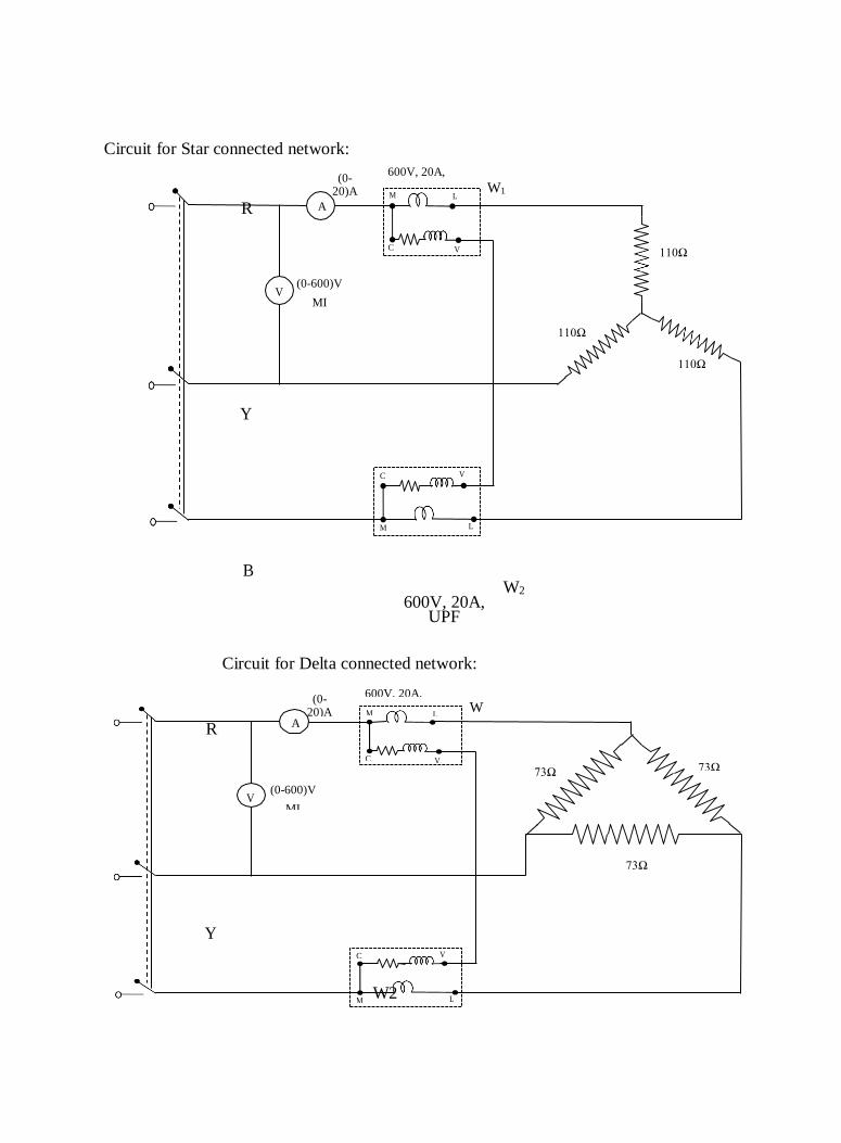
(0-20)A
MI
600V, 20A, UPF M L
W1
A
C V 110Ω
(0-600)V V
MI
110Ω
110Ω
C V
M L
(0-20)A
MI
600V, 20A, UPF M L
W11 A
C V
73Ω 73Ω
(0-600)V V
MI
73Ω
C V
M L
Circuit for Star connected network:
R
Y
B
W2 600V, 20A,
UPF
Circuit for Delta connected network:
R
Y
W2
Procedure:
(Star connection):
7) Connect the circuit as shown in the figure.
8) Ammeter is connected in series with wattmeter whose other end is
connected to one of the loads of the balanced loads.
9) The Y-phase is directly connected to one of the nodes of the 3-ph
supply.
10) A wattmeter is connected across R-phase & Y-phase as shown in fig.
The extreme of B- phase is connected to the third terminal of the
balanced 3-ph load.
11) Another wattmeter is connected across Y & B phase, the extreme of B-
phase is connected to the third terminal of the balanced three phases
load.
12) Verify the connections before switching on the 3-ph power supply.
(Delta connection):
7) Connect the circuit as shown in the figure.
8) Ammeter is connected in series with wattmeter whose other end is
connected to one of the loads of the balanced loads.
9) The Y-phase is directly connected to one of the nodes of the 3-ph
supply.
10) A wattmeter is connected across Y & B phase, the extreme of B-phase
is connected to the third terminal of the balanced 3-ph load.
11) Another wattmeter is connected across R & Yphase, the extreme of R-
phase is connected to the third terminal of the balanced three phases
load.
12) Verify the connections before switching on the 3-ph power supply.
Precautions:
3. Avoid making loose connections.
4. Readings should be taken carefully without parallax error.
Result: