Embed Size (px)
Citation preview

Networks and Systems
Prof. V. G. K. Murti
Department of Electrical Engineering
Indian Institute of Technology, Madras
Lecture - 34
Network Theorems (1)
Superposition Theorem
Substitution Theorem
The next topic, we will take up for discussion is Network Theorems. I am sure that you
had acquaintance with various types of networks theorems in your earlier circuit analysis
courses. Like, the superposition theorem, Thevenin’s theorem, Norton’s theorem and so
on. So, we will have a brief review of the various network theorems. And this will be as I
said a review of, what you are already know.
But, perhaps it will deepen your understanding of the theorems, in one or more respects
in the respect of certain theorems. You may also learn a few additional theorems, which
you have been not exposed to in your earlier courses. But, the normal feature of what we
are going to discuss here, from your point of view. May be the application of these
theorems in the Laplace transform domain, which is of course, a new feature, which you
would not have had in your earlier courses.
Now, network theorems, furnish a particularly simple solutions of network problems in
special cases. So, often times, the solution of a particular problem using the routine
methods, may enter long computation or calculations. But, if you use a particular
theorem, which is relevant to the problem on hand. Then the solution, may become quite
simple and straight forward.
So, after studying the various network theorems, one should develop the facility of
identifying a particular theorem, which fetches us the solution in the most direct and
simple way, from the whole lot of theorem that are available to you. So, this
discrimination and the facility of choosing a particular theorem, relevant to the context is
something very important. Certainly network theorems also provide us special insights
into the network behavior, quite often.
And this is an additional reason why, we study network theorems. As you are aware by
now, there are three main realms of network analysis, using the algebraic method. One is
the DC circuit analysis methods, then the AC circuit analysis methods. Then the methods
using transform diagram in the Laplace transform domain. All these three methods have
a common set of techniques of network analysis.
Whether, you use the loop current method or the node voltage method. The principle, the
essential basics of the network analysis methods are the same in. However, in the case of
DC circuits you write the equations in terms of various constants, which are the
resistance of the network or the conductance of the network. And the variables, which
are DC quantities, which are constants.
In the case of AC circuit analysis, the constants are complex constants and the variables
are the phases of the voltage and currents, which you are trying to solve. In the case of
Laplace transform technique, the equations once again turn out to be algebraic. But, the
coefficients of the various variables that you are trying to solve for are functions of s,
algebraic functions of s. The impedance functions, the admittance functions are the
functions there of. And the variables themselves, which you are trying to solve for are
functions of the complex variables s.
The transform of the voltage, the transform of the current as the case may be. So, all the
three domains. Whether, it is a DC circuit analysis, the AC circuit analysis or the
transform domain, essential techniques are one at the same. However, the details will
vary. And so provided, you pay special attention to the small details, which are
demanded by the requirements of the particular realm. We can be assured that the
general principles, governing the network analysis are the same.
Consequently, the network theorem that we are going to talk about also have validity in
all the three domains. Whether, the DC circuit analysis, AC circuit analysis or the
transform domain. So, what we will do is, try to give the statements of the various
network theorems. And try to discuss them in the most general context, which is the
Laplace transform domain. And it is simplification when, it is the AC circuit analysis or
the DC circuit analysis will be almost evident.
So, let us now start with a review of superposition theorem, which you are sure, all of
them you are familiar with already, in the context of DC circuits or AC circuits.

(Refer Slide Time: 06:47)
The statement, of the superposition theorem would be something like this. In a linear
network, acted upon by several sources. I would say, let us say several independent
sources, the response in any element of the network. Of course, is the sum of the
responses obtained with one source, acting at a time the other sources being deactivated.
Since, I am sure you already know about this. We will not elaborate on this except of
course, to point out that when you have a whole lot of sources acting upon a linear
network, the crucial statement is a linear network.
In a linear network, acted upon by several independent sources then if, you want to
calculate the response in any particular quantity, in a particular element say the voltage
response or current response in a particular element. It is obtained, by the superposition
of the responses, obtained by the individual sources. One each one acting at one time and
when, the particular source is acting all the other sources are deactivated. So, we
specifically mention what is meant by deactivation in a moment.
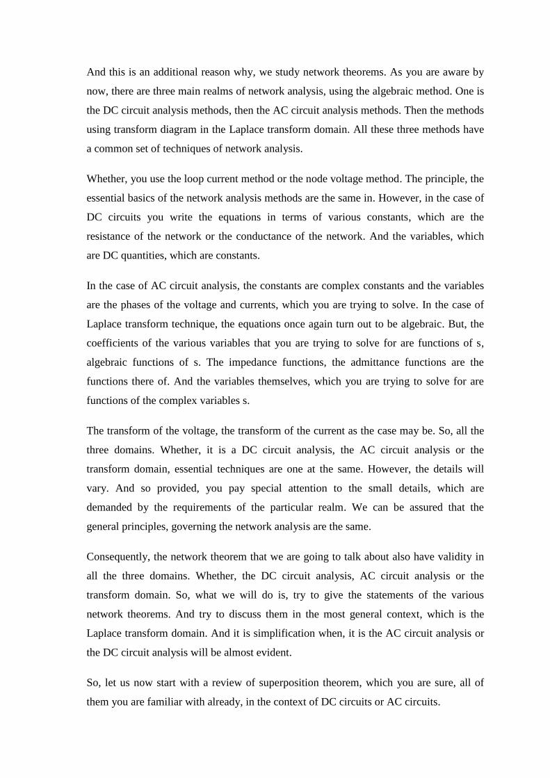
(Refer Slide Time: 09:56)
So, comments on this, is the superposition when you talk about superposition, it may be
you have several sources distributed into the network. So, then you take one source at a
time. It can be superposition of several sources distributed in a network. So, each source
you take at a time. Alternately, if there is a single source, you can decompose that you
can resolve that into several elementary sources, much as we have done in the case of
Fourier analysis.
And consider the effect of each source at a time or superposition of the elementary
sources, into which a single source is resolved. So, in other words, it may be the spatial
distribution of the sources, which you have super positioned or a single source at a given
location, which is resolved into a sum of several elementary resources. And then you
find the effect of each source in turn. So; that means, a temporal or if it is a waveform,
there is a. It may be a particular source, may be resolved into several functions of time
independent functions of time like, a Fourier analysis.
So, the resolution of a periodic waveform into a several sinusoids or it could be
exponential type of distribution, in which you take the effect of one source at a time.

(Refer Slide Time 12:04)
Second comment is deactivation means, voltage sources are replaced by short circuits
because the voltage strength is made equal to 0. That means, a particular voltage source
is replaced by a short circuit. Current sources, if there are any and when you are
considering the effect of other sources, a particular current source is replaced by an open
circuit. Current sources are replaced by open circuit.
In other words, you are reducing the strength of that source whether it is a voltage source
or a current source to 0. So, when you are reducing this strength of voltage source to 0, it
means you are replacing it by a short circuit. If you are replacing this the strength of a
current source, if you are reducing the strength of a current source to 0, it means it is
replaced by an open circuit.
Third point is when we are considering the effect of this various sources at a time, it is
only the independent sources that you should consider, dependent sources if they are any,
they form part of the linear network. A linear network contains, linear elements and the
linear elements include, the dependent sources also because the dependent voltage source
is linearly dependent on the controlling quantity.
(Refer Slide Time: 13:48)
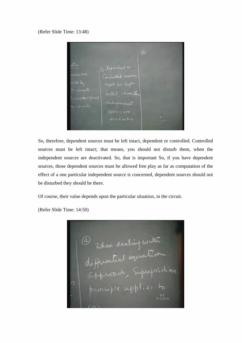
So, therefore, dependent sources must be left intact, dependent or controlled. Controlled
sources must be left intact; that means, you should not disturb them, when the
independent sources are deactivated. So, that is important So, if you have dependent
sources, those dependent sources must be allowed free play as far as computation of the
effect of a one particular independent source is concerned, dependent sources should not
be disturbed they should be there.
Of course, their value depends upon the particular situation, in the circuit.
(Refer Slide Time: 14:50)

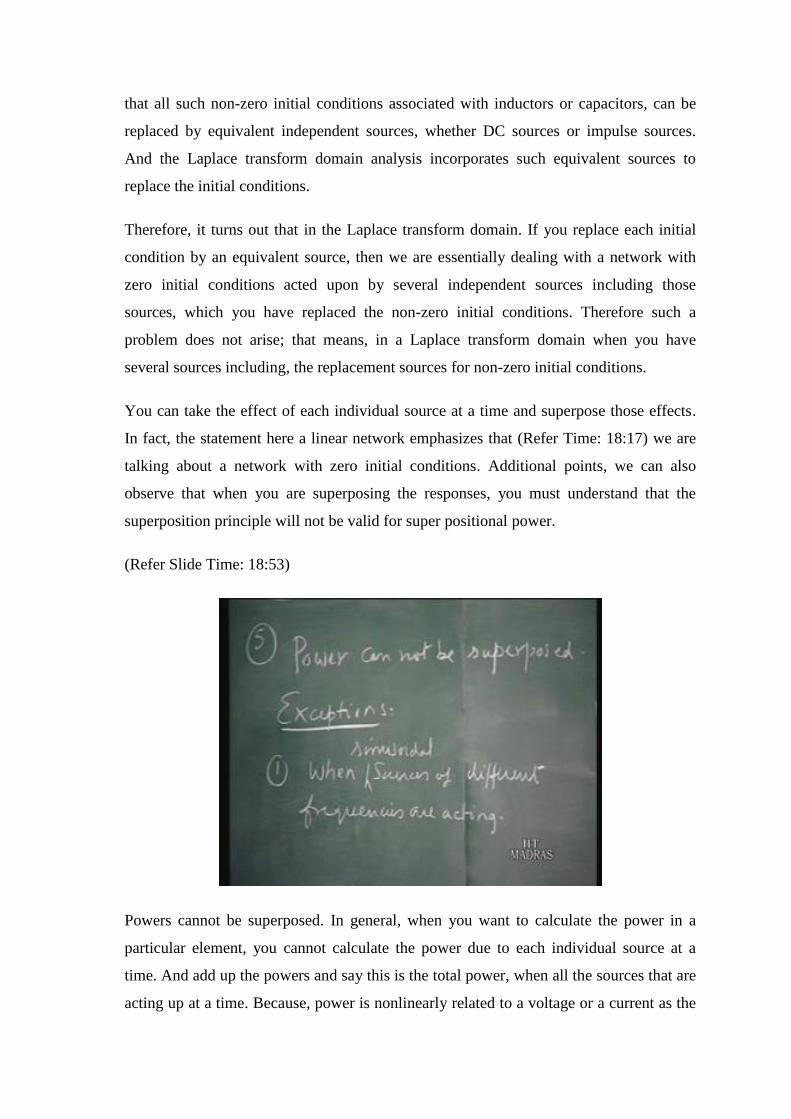
The fourth point, which we should like to observe, is when dealing with differential
equations. When dealing with differential equations, differential equation approach, the
superposition principle applies to a. Suppose, you are taking up a differential equations
approach to solution of a network problem and then you have several sources. And you
consider one source at a time then you would like to find out the response due to leak
source in turn.
Then, you can superpose the responses to the individual sources, provided the response
that you are talking about is a particular integral solution.
(Refer Slide Time: 15:52)
So, superposition will be applicable to particular integral solutions alternately, the total
solution with zero initial conditions. So, you can superpose the responses, if they are in
the form of particular integral solutions or alternately, if the total solution is what you are
looking for and you want to superpose this total solution due to each, individual source
acting at a time. Then the superposition principle is valid, provided the network has zero
initial conditions
This is because, when you have an initial current in an inductor or an initial charge in
capacitor. It spoils the linearity of the terminal relations, of the equations terminal
relations between the voltage and current in an inductor or a capacitor. You may recall,
that all such non-zero initial conditions associated with inductors or capacitors, can be
replaced by equivalent independent sources, whether DC sources or impulse sources.
And the Laplace transform domain analysis incorporates such equivalent sources to
replace the initial conditions.
Therefore, it turns out that in the Laplace transform domain. If you replace each initial
condition by an equivalent source, then we are essentially dealing with a network with
zero initial conditions acted upon by several independent sources including those
sources, which you have replaced the non-zero initial conditions. Therefore such a
problem does not arise; that means, in a Laplace transform domain when you have
several sources including, the replacement sources for non-zero initial conditions.
You can take the effect of each individual source at a time and superpose those effects.
In fact, the statement here a linear network emphasizes that (Refer Time: 18:17) we are
talking about a network with zero initial conditions. Additional points, we can also
observe that when you are superposing the responses, you must understand that the
superposition principle will not be valid for super positional power.
(Refer Slide Time: 18:53)
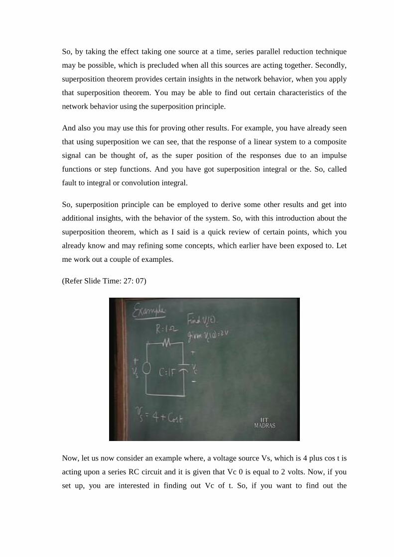
Powers cannot be superposed. In general, when you want to calculate the power in a
particular element, you cannot calculate the power due to each individual source at a
time. And add up the powers and say this is the total power, when all the sources that are
acting up at a time. Because, power is nonlinearly related to a voltage or a current as the

case may be; however, there are special exceptions to this because in such cases, the
power can be superposed.
Exceptions are 1, when sources of different frequencies, when sinusoidal sources of
different frequencies are acting in which case, because as you have seen when we talked
about in fury with short. In terms of a calculation of power, when we are discussing the
Fourier series that the cross products of two different frequency terms. We will have a
zero average therefore, it turns out when sinusoidal source have different frequencies are
acting; you can calculate the power due to each source at a time, each frequency source.
And then superpose them, the total power will can be superposed in this context.
(Refer Slide Time: 20:35)
Secondly, it may arise that when two sources when two sinusoidal sources of the same
frequency, but with a 90 degree phase shift are acting. So, if I have one sinusoid, which
is sin omega t type of thing and the other is cos omega t. You can find out the power due
to each individual source and add them up because, it turns out that the magnitude of a
plus j b is square root of a square plus b square
Therefore, from that relation, you will find that when two sinusoidal sources of same
frequency, but a 90 degree space shift act then also power can be superposed.

(Refer Slide Time: 21:43)
A third interesting situation arises, when a DC network that is a resistor network acted
upon, is acted upon by voltage and current sources.
(Refer Slide Time: 22:29)
Then, the total power delivered by the sources is the sum of powers delivered by voltage
sources alone. And power delivered by the voltage by the sum of power delivered, power
delivered by the voltage sources alone and power delivered by current sources alone.
This is a very special result, which is interesting that if we have several voltage sources

and current sources, acting upon a resistive network then you calculate the total power
delivered by the voltage source acting alone.
All the current sources are open circuited then, let us call that PV then, find out the total
power delivered by the current sources acting with the voltage source deactivated. Let us
call that Pi then the total power is Pv plus Pi, which is the superposition of these two
powers. These are exceptional case, special cases. Then, lastly we might like to ask at
this point, what is the advantage of this superposition theorem, application to
superposition theorem to network analysis.
One answer to this is that, if you have a complicated network acting upon by several
sources. Then the network analysis method that you have to apply, may be a general one
like, the loop current method and the node voltage method, which requires a considerable
algebra. On the other hand, if you are taking only one source at a time. It may be that the
whole network configuration may be one of the series parallel type.
Therefore, the analysis technique that you would employ would be one where, you
combine two elements in series or in parallel and analysis may be that much simpler. So,
this will not be possible if you are two or three other sources plus two or three sources
present at the same time. Therefore, by using the superposition theorem, you may reduce
the complexity of the network or the configuration of the network to a simpler form and
the analysis may be that much faster.
(Refer Slide Time: 25:11)
So, by taking the effect taking one source at a time, series parallel reduction technique
may be possible, which is precluded when all this sources are acting together. Secondly,
superposition theorem provides certain insights in the network behavior, when you apply
that superposition theorem. You may be able to find out certain characteristics of the
network behavior using the superposition principle.
And also you may use this for proving other results. For example, you have already seen
that using superposition we can see, that the response of a linear system to a composite
signal can be thought of, as the super position of the responses due to an impulse
functions or step functions. And you have got superposition integral or the. So, called
fault to integral or convolution integral.
So, superposition principle can be employed to derive some other results and get into
additional insights, with the behavior of the system. So, with this introduction about the
superposition theorem, which as I said is a quick review of certain points, which you
already know and may refining some concepts, which earlier have been exposed to. Let
me work out a couple of examples.
(Refer Slide Time: 27: 07)
Now, let us now consider an example where, a voltage source Vs, which is 4 plus cos t is
acting upon a series RC circuit and it is given that Vc 0 is equal to 2 volts. Now, if you
set up, you are interested in finding out Vc of t. So, if you want to find out the
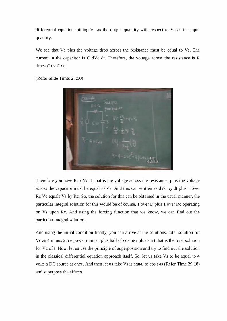
differential equation joining Vc as the output quantity with respect to Vs as the input
quantity.
We see that Vc plus the voltage drop across the resistance must be equal to Vs. The
current in the capacitor is C dVc dt. Therefore, the voltage across the resistance is R
times C dv C dt.
(Refer Slide Time: 27:50)
Therefore you have Rc dVc dt that is the voltage across the resistance, plus the voltage
across the capacitor must be equal to Vs. And this can written as dVc by dt plus 1 over
Rc Vc equals Vs by Rc. So, the solution for this can be obtained in the usual manner, the
particular integral solution for this would be of course, 1 over D plus 1 over Rc operating
on Vs upon Rc. And using the forcing function that we know, we can find out the
particular integral solution.
And using the initial condition finally, you can arrive at the solutions, total solution for
Vc as 4 minus 2.5 e power minus t plus half of cosine t plus sin t that is the total solution
for Vc of t. Now, let us use the principle of superposition and try to find out the solution
in the classical differential equation approach itself. So, let us take Vs to be equal to 4
volts a DC source at once. And then let us take Vs is equal to cos t as (Refer Time 29:18)
and superpose the effects.

(Refer Slide Time: 29:23)
So, if I take Vs as 4 volts. So, you have a 4 volts source and then you have a resistance
and capacitance Vc.
(Refer Slide Time: 29:34)
So, the particular integral solution for that when, you have 4 volts DC, Vc will also be
equal to 4 volts. The complementary function for this Vc will turn out to be minus 2 e to
the power of minus t therefore, the total solution taking Vc 0 to be 2 volts. So, if you take
the total solution, this is particular complementary is also taken with that initial condition
this will turn out to be 4 minus 2 e to the power of minus t volts that is Vc.

(Refer Slide Time: 30:24)
Now, on the other hand you take the source to be a sinusoidal function cos t and then you
have RC network. And if, you have 1 ohm resistance and a 1 farad capacitor, so you find
out the impedance of this. This is cos t, omega equals 1 impedance is 1 minus j that is
root 2 at an angle of minus 45 degrees. So, if cos t is a driving voltage and the impedance
is root 2 at the angle of minus 45 degrees.
(Refer Slide Time: 31:03)
It turns out that the particular integral solution is 0.5 cos t plus sin t, that is the particular
integral solution. And complementary function will turn out to be 1.5 e to the power

minus t. Therefore, the total solution is 1.5 e to the power of minus t plus 0.5 cos t plus
sin t. Now, if you add these, the total particular integral solution is 4 plus 0.5 cos t plus
sin t. If, you take the sum of the total solution this is 4 minus 2 e to power of minus t,
minus 2 e to the power of minus t plus 1.5 minus e t.
So, therefore, 4 minus 0.5 e to the power minus t plus 0.5 cos t plus sin t, this is what you
get. Now, if you compare these two expressions, with the result that you would obtain
under normal calculations, you will observe that 4 plus half cos t is sin t, the particular
integral solution here is the correct one. However, the total solution you have get 4 minus
2.5 e to the power of minus t plus this whereas, here you get 4 minus 0.5 e to the power
minus t.
The discrepancy arose because when, you are calculating this total solution you have
taken the initial capacity voltage to be 2 volts. When you have taken this, the cap with
this the second source, you have taken the initial capacitance voltage once again as 2
volts. Therefore, when you are adding this up, you are getting the initial capacitor
voltage as 4 volts. And that is what this gives when t equals 0.
So, the total solutions will not add up because, you have taken the initial capacitance
voltage as 2 volts. On the other hand, if you have taken the total solution taking the
initial capacitance voltage to be 0 volts, you would get some value. And if you replace
the initial voltage, across the capacitor by an additional DC source of 2 volts then you get
the total solution correct. So, you can work that out, I will leave the details to you.

(Refer Slide Time: 33:36)
Then you take three sources, now you replace the initial capacitor voltage by 2 volt
source; that means, you take a 4 volts DC source here as before then a cos t term, a
resistance here R equals 1 ohms. And the capacitor you replace it by an uncharged
capacitor, plus a 2 volt source represent the initial conditions. And you take this your to
be your Vc and calculate this Vc using this source as one time and this source as another
time, you will get the correct solution, even if you superpose the total solution.
So, that is what we meant earlier that you can superpose the total solutions with 0 initial
conditions, because now this capacitor is assumed to have 0 voltages. Because whatever,
non-zero initial conditions was there it is replaced by the equivalent source. Let us take
another example.
(Refer Slide Time: 34:32)
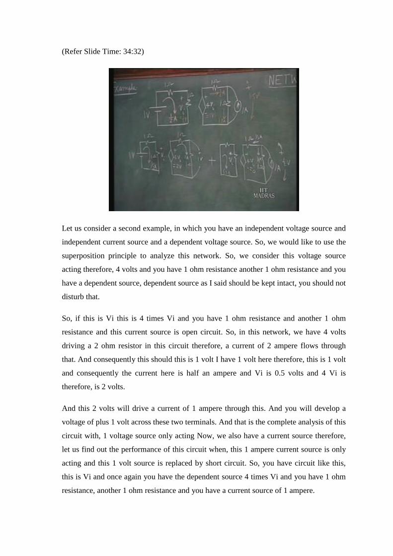
Let us consider a second example, in which you have an independent voltage source and
independent current source and a dependent voltage source. So, we would like to use the
superposition principle to analyze this network. So, we consider this voltage source
acting therefore, 4 volts and you have 1 ohm resistance another 1 ohm resistance and you
have a dependent source, dependent source as I said should be kept intact, you should not
disturb that.
So, if this is Vi this is 4 times Vi and you have 1 ohm resistance and another 1 ohm
resistance and this current source is open circuit. So, in this network, we have 4 volts
driving a 2 ohm resistor in this circuit therefore, a current of 2 ampere flows through
that. And consequently this should this is 1 volt I have 1 volt here therefore, this is 1 volt
and consequently the current here is half an ampere and Vi is 0.5 volts and 4 Vi is
therefore, is 2 volts.
And this 2 volts will drive a current of 1 ampere through this. And you will develop a
voltage of plus 1 volt across these two terminals. And that is the complete analysis of this
circuit with, 1 voltage source only acting Now, we also have a current source therefore,
let us find out the performance of this circuit when, this 1 ampere current source is only
acting and this 1 volt source is replaced by short circuit. So, you have circuit like this,
this is Vi and once again you have the dependent source 4 times Vi and you have 1 ohm
resistance, another 1 ohm resistance and you have a current source of 1 ampere.
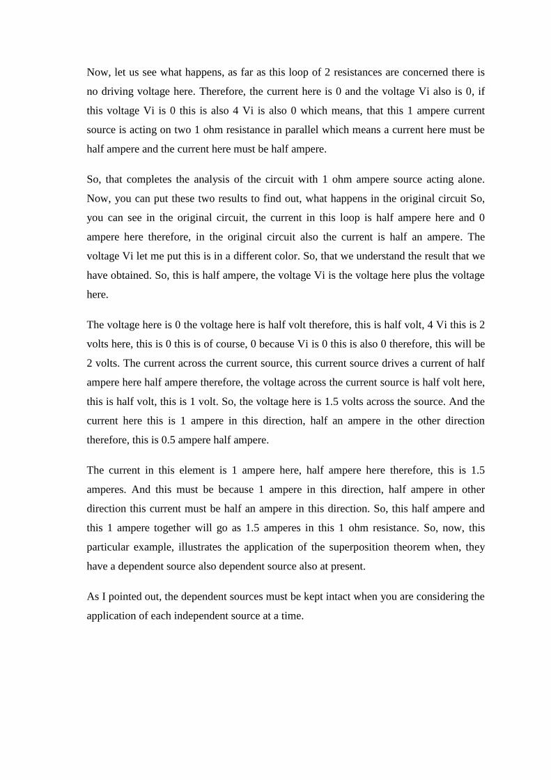
Now, let us see what happens, as far as this loop of 2 resistances are concerned there is
no driving voltage here. Therefore, the current here is 0 and the voltage Vi also is 0, if
this voltage Vi is 0 this is also 4 Vi is also 0 which means, that this 1 ampere current
source is acting on two 1 ohm resistance in parallel which means a current here must be
half ampere and the current here must be half ampere.
So, that completes the analysis of the circuit with 1 ohm ampere source acting alone.
Now, you can put these two results to find out, what happens in the original circuit So,
you can see in the original circuit, the current in this loop is half ampere here and 0
ampere here therefore, in the original circuit also the current is half an ampere. The
voltage Vi let me put this is in a different color. So, that we understand the result that we
have obtained. So, this is half ampere, the voltage Vi is the voltage here plus the voltage
here.
The voltage here is 0 the voltage here is half volt therefore, this is half volt, 4 Vi this is 2
volts here, this is 0 this is of course, 0 because Vi is 0 this is also 0 therefore, this will be
2 volts. The current across the current source, this current source drives a current of half
ampere here half ampere therefore, the voltage across the current source is half volt here,
this is half volt, this is 1 volt. So, the voltage here is 1.5 volts across the source. And the
current here this is 1 ampere in this direction, half an ampere in the other direction
therefore, this is 0.5 ampere half ampere.
The current in this element is 1 ampere here, half ampere here therefore, this is 1.5
amperes. And this must be because 1 ampere in this direction, half ampere in other
direction this current must be half an ampere in this direction. So, this half ampere and
this 1 ampere together will go as 1.5 amperes in this 1 ohm resistance. So, now, this
particular example, illustrates the application of the superposition theorem when, they
have a dependent source also dependent source also at present.
As I pointed out, the dependent sources must be kept intact when you are considering the
application of each independent source at a time.
(Refer Slide Time: 39:42)
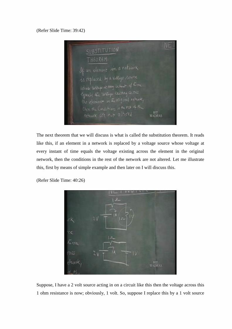
The next theorem that we will discuss is what is called the substitution theorem. It reads
like this, if an element in a network is replaced by a voltage source whose voltage at
every instant of time equals the voltage existing across the element in the original
network, then the conditions in the rest of the network are not altered. Let me illustrate
this, first by means of simple example and then later on I will discuss this.
(Refer Slide Time: 40:26)
Suppose, I have a 2 volt source acting in on a circuit like this then the voltage across this
1 ohm resistance is now; obviously, 1 volt. So, suppose I replace this by a 1 volt source

and consider this network 2 volts 1 ohm then the current in the network, everything else
will remain the same, here we have a 1 ohm, 1 ampere current here also you have 1
ampere current. The voltage across this resistance here and here are the same; that
means, this element which had a 1 volts potential drop across this is replaced by a
source. So, that is the statement of this theorem.
(Refer Slide Time: 41:20)
In general, you have a network here and let us say that we have an element here, may be
linear, may be non-linear that element we have not made in this particular stipulation. It
has in the Laplace transform domain let us say it has a voltage Vs. And it has a certain
current, I of s. Now, what this substitution theorem tells us is that in this network, if you
replace this element by a voltage source whose voltage is Vs, which is the same as this
then all the other conditions in the network will remain the same.
Suppose, I have an element here, whose voltage is Vk and whose current is Ik in this will
continue to be Vk and the current will be Ik. What is the justification for this,
justification is that if you are doing the node voltage method of analysis. Let us take this
as datum node, take this as the datum node then the node equations at all other nodes
inside the network will remain the same.
As far as this node is concerned, (Refer Time: 42:32) in the original network V of s is the
solution for this node voltage. Now, here we are stipulating that node voltage to be Vs.
So, this node voltage stipulation is consistent with the solution that is obtained in the

original network. The other node equations are the same, for this particular node you are
giving the solution itself as the data therefore, it is consistent. Therefore, whatever
solution you have obtained here, will be the same as this as far the other nodes are
concerned.
Similarly, if you are using the loop equations, the other loop equations are the same. In
this loop equation corresponding to I of s across this in particular element you have some
fair example, as Zs I of s something would have written. And now whatever, solution
you had obtained for this is now incorporated here. So, this stipulation for this loop
equation is consistent with the solution, the other loop equations are the same. Therefore,
the solution for the other element responses will be the same this is the principle of the
substitution theorem.
Now, there were couples of points, which I would like to emphasize here. We do not
have a tremendous advantage in using the substitution theorem to solve the network
problems. However, it turns out to be very useful, in proving some other theorems using
the substitution principle we can use several other theorems. Also in some cases where,
the switches are opened and closed you can apply the substitution theorem and get
special insights in the circuit behavior and also the total solution with fairly straight
forward fashion. So, that is the usefulness of the substitution theorem.
Second point I would like to emphasize is that the element that you are replacing, can be
linear or non-linear does not matter what it is. A third point is when you replace for
example, when you in this particular let us take the same case here.

(Refer Slide Time: 44:30)
Suppose, I have a similar case, I mean not the same case suppose I have a case here you
have a 2 volt source acting upon a 1 ohm resistance. So, the voltage across this is 2 volts.
Now, suppose you replace this 1 ohm resistor by another 2 volt source. So, we have this
resultant circuit and what is the current in this. It can be anybody’s guess, because this is
a particular type of circuit, in which any current I is a possible solution. So, this network
we can say is not solvable, because you do not have a definite solution for this network.
So, we have used this substitution theorem, this is the one particular solution which is
equal to 2 amperes is also solution, but that is not a definite solution for this network.
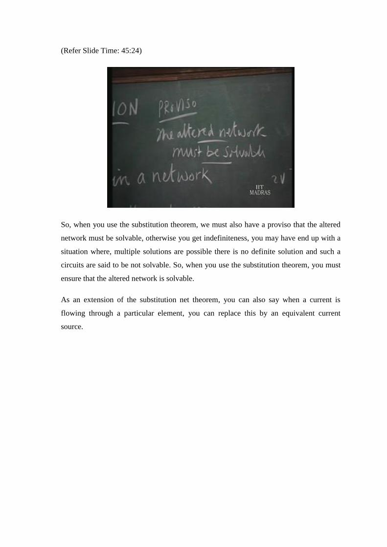
(Refer Slide Time: 45:24)
So, when you use the substitution theorem, we must also have a proviso that the altered
network must be solvable, otherwise you get indefiniteness, you may have end up with a
situation where, multiple solutions are possible there is no definite solution and such a
circuits are said to be not solvable. So, when you use the substitution theorem, you must
ensure that the altered network is solvable.
As an extension of the substitution net theorem, you can also say when a current is
flowing through a particular element, you can replace this by an equivalent current
source.

(Refer Slide Time: 46:08)
So, you can also have a current source I of s. This is alternative form of substitution
theorem you can replace this particular element by a current source, whose value at every
instant of time is the current in the original network. So, you can replace this element by
a voltage source or a current source. This is also a substitution theorem, which is an
alternate version of the main theorem in which, we said an element can be replaced by a
voltage source.
As I mentioned, the substitution theorem gives us some special insights in circuit
behavior when, particularly when switches are opened and closed, which we will see in
later. And it is also used to prove several other theorems this is the special advantage of
the substitution theorem. So, in this lecture, we have started the discussion of various
network theorems. I mentioned, network theorems are used to simplify the analysis of
networks, in particular cases. And depending upon the problem on hand, one of the
network theorems may be quite appropriate to apply it provides us a solution in a straight
forward fashion.
So, we should develop the ability to choose the particular theorem, which facilitates the
solution in the most effective way in a given situation. And we talked about
superposition theorem, in which we said the response of a particular element situated in a
network linear network. When it is acted upon by several independent sources, can be
obtained by finding out the response in that element with each source acting in turn,
keeping all the other source as deactivated. And superposing, the individual responses to
get the total response.
We mentioned that in the case of deactivation, what we mean by deactivation is that the
voltage source strength is reduced to 0 and current source strength is reduced to 0 which
means, that the voltage is replaced by the short circuit, the current is replaced by an open
circuit. And this is to be done for all independent sources, dependent source if they are
any must be kept intact, they are part of the linear system.
Secondly we observe that when you want to find out that transient solution in a network.
Then, the superposition principle can be applied with 0 initial conditions in the system or
with all initial conditions replaced by equivalent sources. And therefore, the principle of
superposition can be extended to the sources, which stand for the non-zero initial
conditions. And this is what we do in the Laplace transform domain where, non-zero
initial conditions are replaced by equivalent sources.
We also mentioned that the superposition principle, will be can prove to be effective,
when we are when we take one source at a time, the network configuration becomes
simpler like in the series parallel structure. Then, we can use the analysis with each
source in turn by request taking request simplify it in form of network analysis, provided
by this series parallel structure, where as if you had more than one source such a series
parallel reduction technique may not be possible.
We observed that power cannot be superposed in general, but there are few exception,
which we pointed out. Then, we discuss the so called substitution theorem where, in a
given network. If, you so choose a particular element can be replaced by a current source
or a voltage source. The current source being having a value, which is equal at every
instant of time to the actual current that, was existing in network, original network and
similarly the voltage source.
Then the question that you will naturally ask is if, you know the current in the network
then what is the purpose of using a network theorem to follow for it. The answer to that
is, we do not use the substitution theorem to find out the current in a network in most of
the appropriate cases. We use this as a kind of artifices or tactic to prove other network
theorems.

Also in some cases, it turns out that where, you are opening or closing the switches
replacement of an open or a close switch by a suitable current source or a voltage source
as we will see, will be effective in providing us a solution, which is a straight forward
one. We will discuss other network theorems, in the next lecture. But, before that let me
mention that we a third network theorem, which is called the reciprocity theorem is
something which you have already discussed.
And you can just read right, now that if in a linear reciprocal network, which consist of
bilateral elements and reciprocal elements. The ratio of the Laplace transform, the
response emolument, response to the excitation Laplace transform is the same when, the
locations of the response and the excitation are interchanged. This is true in a network
containing bilateral elements and reciprocal elements, this is a something which we have
already discussed, when we talked when we have discussing the two port network
characteristics.
So, we will not discuss reciprocity theorem specially, here as one of the network
theorems. This we will assume as already being discussed with this, but; however, some
ramifications of reciprocity theorem will be discussed, when we talk about Thevenis’s
theorem at a later point of time.