Embed Size (px)
Citation preview
NETWORKED CONTROL SYSTEMS:EMULATION-BASED DESIGN
MOHAMMAD TABBARA, DRAGAN NESIC AND ANDREW R. TEEL
Abstract. A common approach to the implementation of digi-tal systems is through the emulation of idealized continuous-timeblocks in order to be able to leverage the rich expanse of re-sults and design tools available in the continuous-time domain.So called sampled-data systems are now commonplace in prac-tice and rely upon results that ensure that many properties ofthe nominal continuous-time system, including notions of stability,are preserved under sampling when certain conditions are verified.In analogy with (fast) sampled-data design, this chapter exploresan emulation-based approach to the analysis and design of net-worked control systems (NCS). To that end, we survey a selec-tion of emulation-type NCS results in the literature and highlightthe crucial role that scheduling between disparate components ofthe control systems plays, above and beyond sampling. We detailseveral different properties that scheduling protocols need to ver-ify together with appropriate bounds on inter-transmission timessuch that various notions of input-output stability of the nominal“network-free” system are preserved when deployed as an NCS.
1. Introduction
Control of a system is to influence its behavior to achieve a desiredgoal, often, through the use of feedback. Diagrammatically, we areoften concerned with the setup depicted in Figure 1: analysis of plantP with (vector) output y and design of a controller C with a (vector)control u to achieve a desired closed-loop behavior, typically, a notionof stability.
C Py u
Figure 1. Conceptual Block diagram of Feedback Control.
The interconnection of physical signals between controller and plantis seldom as elementary as that depicted in Figure 1. Many propertiesof the plant including its physical size, complexity and mobile nature
1
2 MOHAMMAD TABBARA, DRAGAN NESIC AND ANDREW R. TEEL
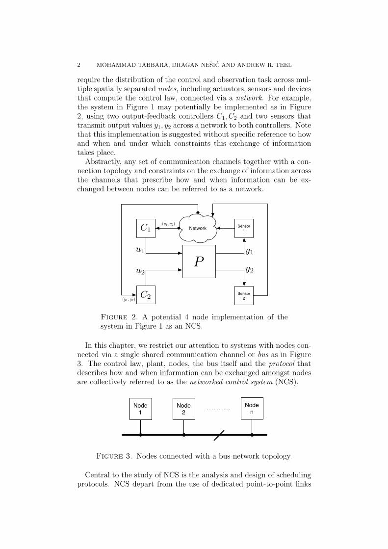
require the distribution of the control and observation task across mul-tiple spatially separated nodes, including actuators, sensors and devicesthat compute the control law, connected via a network. For example,the system in Figure 1 may potentially be implemented as in Figure2, using two output-feedback controllers C1, C2 and two sensors thattransmit output values y1, y2 across a network to both controllers. Notethat this implementation is suggested without specific reference to howand when and under which constraints this exchange of informationtakes place.
Abstractly, any set of communication channels together with a con-nection topology and constraints on the exchange of information acrossthe channels that prescribe how and when information can be ex-changed between nodes can be referred to as a network.
Sensor 2
Sensor 1
Pu1
u2 y2
y1
C2
C1 Network
(y1, y2)
(y1, y2)
Figure 2. A potential 4 node implementation of thesystem in Figure 1 as an NCS.
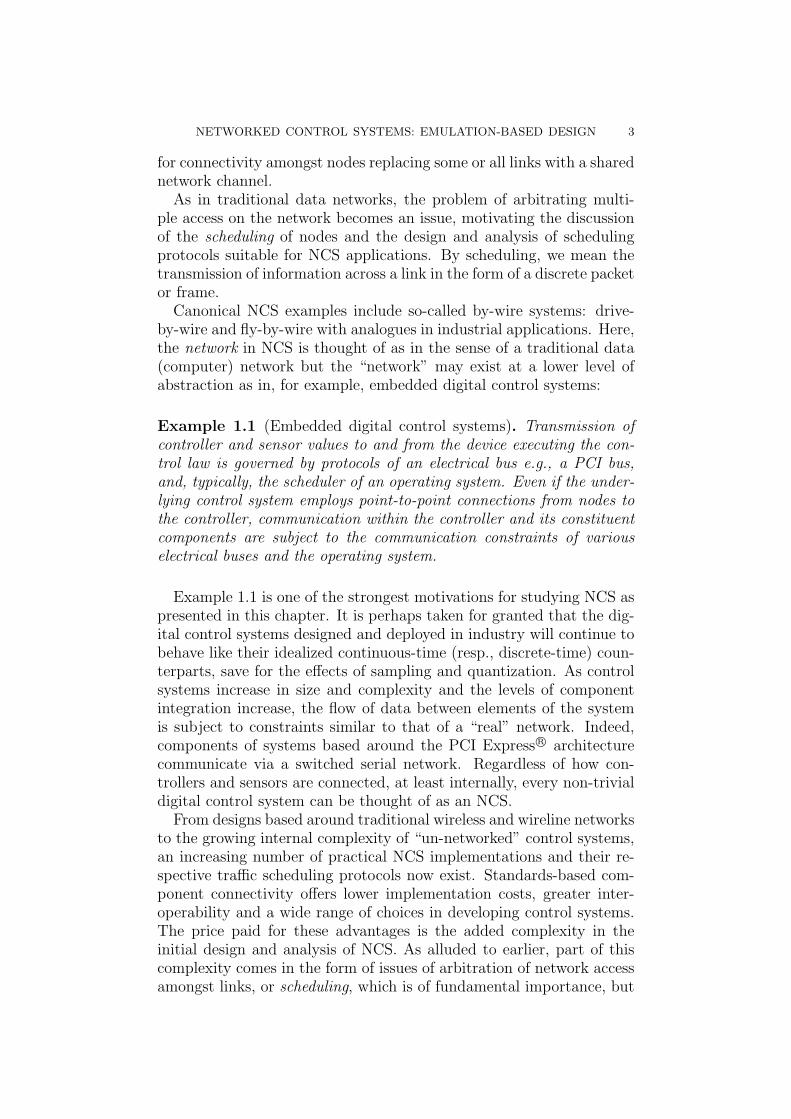
In this chapter, we restrict our attention to systems with nodes con-nected via a single shared communication channel or bus as in Figure3. The control law, plant, nodes, the bus itself and the protocol thatdescribes how and when information can be exchanged amongst nodesare collectively referred to as the networked control system (NCS).
Node 1
Node2
Noden
Figure 3. Nodes connected with a bus network topology.
Central to the study of NCS is the analysis and design of schedulingprotocols. NCS depart from the use of dedicated point-to-point links
NETWORKED CONTROL SYSTEMS: EMULATION-BASED DESIGN 3
for connectivity amongst nodes replacing some or all links with a sharednetwork channel.
As in traditional data networks, the problem of arbitrating multi-ple access on the network becomes an issue, motivating the discussionof the scheduling of nodes and the design and analysis of schedulingprotocols suitable for NCS applications. By scheduling, we mean thetransmission of information across a link in the form of a discrete packetor frame.
Canonical NCS examples include so-called by-wire systems: drive-by-wire and fly-by-wire with analogues in industrial applications. Here,the network in NCS is thought of as in the sense of a traditional data(computer) network but the “network” may exist at a lower level ofabstraction as in, for example, embedded digital control systems:
Example 1.1 (Embedded digital control systems). Transmission ofcontroller and sensor values to and from the device executing the con-trol law is governed by protocols of an electrical bus e.g., a PCI bus,and, typically, the scheduler of an operating system. Even if the under-lying control system employs point-to-point connections from nodes tothe controller, communication within the controller and its constituentcomponents are subject to the communication constraints of variouselectrical buses and the operating system.
Example 1.1 is one of the strongest motivations for studying NCS aspresented in this chapter. It is perhaps taken for granted that the dig-ital control systems designed and deployed in industry will continue tobehave like their idealized continuous-time (resp., discrete-time) coun-terparts, save for the effects of sampling and quantization. As controlsystems increase in size and complexity and the levels of componentintegration increase, the flow of data between elements of the systemis subject to constraints similar to that of a “real” network. Indeed,components of systems based around the PCI Express R© architecturecommunicate via a switched serial network. Regardless of how con-trollers and sensors are connected, at least internally, every non-trivialdigital control system can be thought of as an NCS.
From designs based around traditional wireless and wireline networksto the growing internal complexity of “un-networked” control systems,an increasing number of practical NCS implementations and their re-spective traffic scheduling protocols now exist. Standards-based com-ponent connectivity offers lower implementation costs, greater inter-operability and a wide range of choices in developing control systems.The price paid for these advantages is the added complexity in theinitial design and analysis of NCS. As alluded to earlier, part of thiscomplexity comes in the form of issues of arbitration of network accessamongst links, or scheduling, which is of fundamental importance, but
4 MOHAMMAD TABBARA, DRAGAN NESIC AND ANDREW R. TEEL
above and beyond scheduling, NCS also presents the designer with thelimitations of
(a) finite bandwidth of communication channels;(b) finite precision of encoding and decoding schemes for transmitted
information;(c) pure (propagation) delays of channels;(d) and data dropouts from unreliable channels.
These limitations are not mutually exclusive, however. As transmis-sion rates increase and, with frame and packet sizes well in excess ofmachine (CPU) precision, effects of quantization and pure delay playan increasingly diminishing role in the analysis of most NCS and weforego their consideration in this chapter. We will, however, examinemodels of data dropouts and unreliable channels with Ethernet andso-called p-persistent collision-sense multiple access (CSMA) as primeexamples of such channels.
2. Overview of emulation-based NCS design
2.1. Principles of emulation-based NCS design. As stated in theintroduction, scheduling and scheduling protocols are an integral partof NCS design. A survey of scheduling and various scheduling protocolsis provided in [1] and stability and performance results of NCS havebeen examined in [1–6]. An elementary example of a scheduling pro-tocol, round-robin (RR), grants network access to NCS components insequential, round-robin fashion and is used almost exclusively in prac-tice. The aforementioned works present various alternative protocolsthat demonstrate a performance gain over RR in simulations and, inspecial cases, demonstrate the superiority of the alternative protocolsanalytically. The NCS design approach adopted in [2, 3, 5–7] and [8],and this chapter consists of the following steps:
(a) design a stabilizing controller ignoring the network;(b) choose an appropriate scheduling protocol;(c) and analyze the robustness of stability with respect to effects that
scheduling within a network introduce.
The principal advantage of this approach is its simplicity – the designerof the NCS can exploit familiar tools for controller design and selectan appropriate scheduling protocol and transmission rate such that thedesired properties of the network-free system are preserved.
This chapter will introduce and characterize the various classes ofadmissible protocols for which stability results are developed but it isimportant to note that when the network-free system verifies a nomi-nal stability property and an admissible protocol is chosen, stability ofthe resultant NCS can be achieved through sufficiently high transmis-sion rates (or equivalently, sufficiently low inter-transmission times).
NETWORKED CONTROL SYSTEMS: EMULATION-BASED DESIGN 5
Moreover, stability (robustness) properties of the NCS are actually pa-rameterized by the transmission rate and, hence, step (c) in the designprocess can be reinterpreted as:
(ci) choose a transmission rate (above requisite minimum) to achievea desired degree of robust stability.
Results will be presented where this design approach is adopted withvarious notions of transmission rate (minimum or expected) and robuststability (uniform global exponential or asymptotic stability, Lp or Lp
in-expectation or input-to-state stability).
2.2. Results in Perspective. Consider the following LTI control sys-tem:
xP = APxP +BPu xC = ACxC +BCy(1)
y = CPxP u = CCxC ,(2)
where xP , xC , y and u denote, respectively, plant state, controller state,plant output and control. In the presence of a network and an associ-ated scheduling protocol, y and u cannot be continuously transmittedbetween the plant and controller. The network introduces the followinglimitations:
(a) transmissions occur only at specific transmission instants ti∞i=0;and
(b) only one logical component of the NCS is allowed to transmit(broadcast) data onto the network at a given transmission instant tie.g., for a 3-output 2-input system, one component of y = (y1, y2, y3),u = (u1, u2) can be transmitted.
Let y denote the “stand-in” for y available to and maintained by thedevice(s) that compute the control law and u denote the “stand-in” foru available to and maintained by the device(s) that actuate the plant.In effect, the NCS for the network-free system is described by
xP = APxP +BP u xC = ACxC +BC y(3)
y = CPxP u = CCxC .(4)
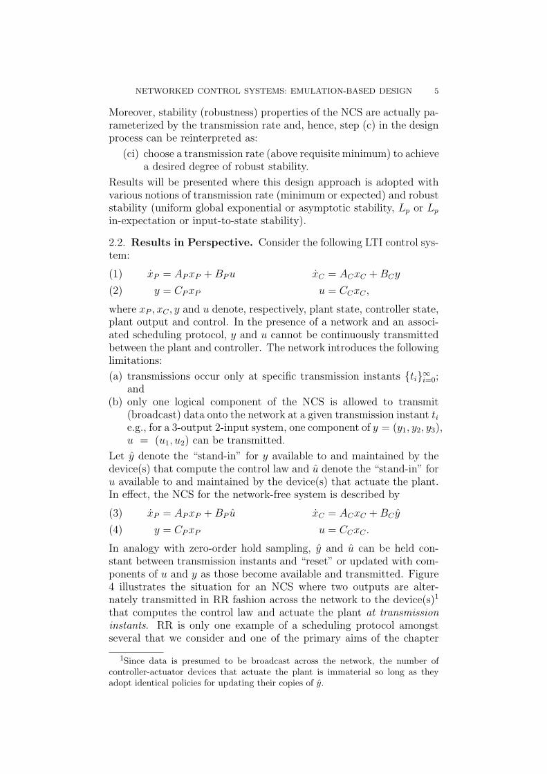
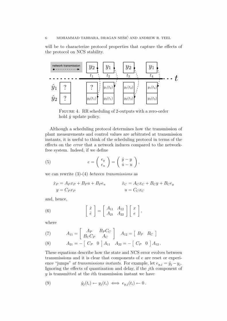
In analogy with zero-order hold sampling, y and u can be held con-stant between transmission instants and “reset” or updated with com-ponents of u and y as those become available and transmitted. Figure4 illustrates the situation for an NCS where two outputs are alter-nately transmitted in RR fashion across the network to the device(s)1
that computes the control law and actuate the plant at transmissioninstants. RR is only one example of a scheduling protocol amongstseveral that we consider and one of the primary aims of the chapter
1Since data is presumed to be broadcast across the network, the number ofcontroller-actuator devices that actuate the plant is immaterial so long as theyadopt identical policies for updating their copies of y.
6 MOHAMMAD TABBARA, DRAGAN NESIC AND ANDREW R. TEEL
will be to characterize protocol properties that capture the effects ofthe protocol on NCS stability.
y1
y2 ?
y1y2 y2 y1
t1 t2 t3 t4
? ?y2(t1) y2(t1)
y1(t2) y1(t2)
y2(t3) y2(t3)
y1(t4)
network transmission
t
Figure 4. RR scheduling of 2-outputs with a zero-orderhold y update policy.
Although a scheduling protocol determines how the transmission ofplant measurements and control values are arbitrated at transmissioninstants, it is useful to think of the scheduling protocol in terms of theeffects on the error that a network induces compared to the network-free system. Indeed, if we define
(5) e =
(ey
eu
)=
(y − yu− u
),
we can rewrite (3)-(4) between transmissions as
xP = APxP +BPu+BP eu xC = ACxC +BCy +BCey
y = CPxP u = CCxC
and, hence,
(6)
[xe
]=
[A11 A12
A21 A22
] [xe
],
where
A11 =
[AP BPCC
BCCP AC
]A12 =
[BP BC
](7)
A21 = −[CP 0
]A11 A22 = −
[CP 0
]A12 .(8)
These equations describe how the state and NCS error evolves betweentransmissions and it is clear that components of e are reset or experi-ence “jumps” at transmissions instants. For example, let ey,j = yj−yj.Ignoring the effects of quantization and delay, if the jth component ofy is transmitted at the ith transmission instant we have
(9) yj(ti)← yj(ti) ⇐⇒ ey,j(ti)← 0 .
NETWORKED CONTROL SYSTEMS: EMULATION-BASED DESIGN 7
Hence, the effect of the scheduling protocol is to reset components of theNCS error2 at transmission instants. An NCS model in this fashion isthus completely prescribed by:
(a) NCS continuous-time dynamics as in (6) and depicted conceptuallyin Figure 5;
(b) a sequence of increasing transmission instants ti∞i=0; and(c) a scheduling protocol, or error reset map that is described via its
effect on the error, e, at transmission instants.
Regarding the NCS continuous-time dynamics as fixed, we would liketo characterize the sequence of transmission instants or, equivalently,the sequence of inter-transmission intervals and the set of protocols forwhich we can conclude that the NCS state (x, e) is stable in an appro-priate sense. The origins of emulation-based NCS design in this sensebegin with the pioneering work of Walsh et al. in [5] and [3] whereNCS models in the form of (6) and its nonlinear counterpart werepresented, together with conditions on the maximum allowable trans-mission interval (MATI) such that the resultant NCS was uniformlyglobally asymptotic or exponentially stable (UGES, UGAS) when us-ing the RR or maximum-error-first try-once-discard (TOD) schedulingprotocols. We defer a detailed discussion of these and other protocolsuntil Section 3.2 and outline results in the spirit of those presentedin [3–5].
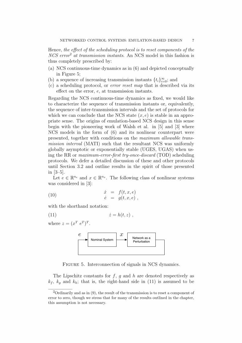
Let e ∈ Rne and x ∈ Rnx . The following class of nonlinear systemswas considered in [3]:
(10)x = f(t, x, e)e = g(t, x, e) ,
with the shorthand notation:
(11) z = h(t, z) ,
where z = (xT eT )T .
Nominal System Network as a Perturbation
e x
Figure 5. Interconnection of signals in NCS dynamics.
The Lipschitz constants for f , g and h are denoted respectively askf , kg and kh; that is, the right-hand side in (11) is assumed to be
2Ordinarily and as in (9), the result of the transmission is to reset a component oferror to zero, though we stress that for many of the results outlined in the chapter,this assumption is not necessary.
8 MOHAMMAD TABBARA, DRAGAN NESIC AND ANDREW R. TEEL
globally Lipschitz, uniformly in t. The class of linear systems (6) withthe obvious shorthand:
(12) z = Az
was considered in [4, 5].It is supposed in [3] that there exists a continuously differentiable
Lyapunov function V such that the system (10) satisfies:
c1|x|2 ≤ V (t, x) ≤ c2|x|2 for all x ∈ Rnx ,(13)
∂V
∂t+∂V
∂xf(t, x, 0) ≤ −c3|x|2 for almost all x ∈ Rnx ,(14) ∣∣∣∣∂V∂x
∣∣∣∣ ≤ c4 |x| ,(15)
where c1, c2, c3, c4 are positive constants. A similar condition was usedin [4,5] for the linear system (6). Indeed, it was assumed that for somepositive definite and symmetric matrix Q there exists a positive definiteand symmetric matrix P that solves the Lyapunov matrix equation3:
(16) AT11P + PA11 = −Q .
It is obvious that (16) implies that (13), (14), (15) are satisfied for thelinear system (6), V (x) = xTPx and
(17) c1 = λmin(P ); c2 = λmax(P ); c3 = λmin(Q) ; c4 = 2λmax(P ),
where λmin(·) and λmin(·) denote the minimum and maximum singularvalue of a symmetric matrix, respectively. For linear systems, we canlet
(18) kh = kf = kg = |A| .
A bound on MATI that guarantees the stability of the linear system(6) with the RR and TOD protocols was obtained in [4,5]. We denotebounds computed in [4, 5] respectively as τRR
∗ and τTOD∗ for the RR
and TOD protocols. Similar bounds were obtained in [3] for nonlin-ear systems (10) with the RR and TOD protocols, where4 the boundsobtained are also such that τRR
∗ = τTOD∗ . The bounds in [3–5] can be
expressed as:
τRR∗ = τTOD
∗ =c3
M`(`+ 1)khkfc4.(19)
3The results in [5] are only presented for the special case Q = I. The result withgeneral Q is presented in [4].
4Note that we do not use different notation for MATI bounds for linear andnonlinear systems, although they are different in general. This is because it alwayswill be always clear from the context which bound we mean.
NETWORKED CONTROL SYSTEMS: EMULATION-BASED DESIGN 9
where the value of the constant M is different for linear and nonlinearsystems and ` denotes the number of nodes that participate in sched-uling. For nonlinear systems, we have
(20) M = MNL = 16
(c2c1
)3/2(√c2c1
+ 1
),
established in [3]. Analogously in [4, 5], the following is obtained forlinear systems
(21) M = ML = 8
√λmax(P )
λmin(P )
(√λmax(P )
λmin(P )+ 1
),
where the meaning of all constants in (19) is explained through (17)and (18). These MATI bounds obtained in [3–5] do not differentiatebetween RR and TOD; that is τTOD
∗ = τRR∗ .
In general, intuition suggests that MATI bounds should be protocol-dependent. Significant improvements upon these MATI bounds weremade in [2] by efficiently capturing protocols properties through protocol-specific Lyapunov functions and characterizing the effects of transmis-sion errors through Lp gains. Essentially, UGES and Lp input-outputstability is with a MATI of:
0 < τ <1
Lln
(1 +
1− θγL
+ θ
),(22)
where θ ∈ [0, 1) characterizes the the ability of the protocol to re-duce network error at transmission instants while L > 0 describes thespeed of the network-error dynamics, and γ > 0 captures the effect ofnetwork-error on the behavior of the ideal system through an Lp gain.In particular, τ is protocol-dependent through θ – the better the pro-tocol is at reducing network-error at transmission instants, the largerthe MATI bound is and, hence, the less frequent transmissions have tobe to guarantee stability of the NCS.
3. Modeling Networked Control Systems & SchedulingProtocols
The premise of networked control systems (NCS) is to spatially dis-tribute a “traditional” control system across a number of nodes thatexchange data subject to the constraints of a shared data channel.These nodes include sensors, actuators and units that compute variouscontrol laws and the data channel is typically a wireless or wirelinecomputer network, many examples of which can be found in [9].
Computer networks and communications systems present rich andsophisticated models of varying degrees of complexity, within stochasticand deterministic settings, and of various underlying physical commu-nication media. For the vast majority of computer networks describedin [9], the primary constraint on the exchange of data between nodes
10 MOHAMMAD TABBARA, DRAGAN NESIC AND ANDREW R. TEEL
is that the respective channels are exclusive. This means that the at-tempt of more than one node to transmit data at a given time willresult in data loss, i.e., a collision. Collisions can be prevented by arbi-tration of network access through the use of scheduling protocols thatdecide which node(s) can transmit and at what times.
The network models presented in this chapter aim to capture theessential aspects of control over networks in the context of several im-portant settings:
(a) locally5 arbitrated network access without packet dropouts;(b) arbitrated network access with and without packet dropouts; and(c) unarbitrated network access with and without packet dropouts.
Arbitration takes place through the use of a scheduling protocoladopted by every node in the network. A protocol can be thoughtof as a map
(23) h : W → 1, .., `that selects the node currently being allowed to transmit and an associ-ated dynamical system that evolves the scheduler state variable ω ∈ W .For spatially separated nodes, this generally means that each node mustmaintain a copy of the state ω that is evolved identically by the node(local knowledge with globally-known inputs), or, ω is known globallyand updated in a distributed fashion. Such protocols are often referredto as contentionless protocols. For example, labeling the NCS nodesa1, a2, ..., a`, round-robin scheduling would entail apportioning thechannel’s time, [0,∞), into slots s1 := [t0, t1), s2 := [t1, t2), . . . , suchthat node ai is permitted to transmit during slot si+k`, k = 0, 1, . . . .Depending on the context, this scheduling protocol is also known astime-division multiplexing or Token Ring and relies on each node be-ing able to count transmissions. In this case,
ω = number of transmissions from some initial time.
For networks with a large number of nodes, mobile nodes that arespatially separated across varying distances or networks with a varyingnumber of nodes, it may be impractical or impossible to keep ω, thestate information, synchronized across all nodes.
The alternative is unarbitrated access in the sense that there is noglobal policy to enforce exclusive network access for a given node ata transmission instant. In particular, collisions may occur, and haveto be detected and recovered from. The number that occur can of-ten be reduced by employing various heuristics using data available toeach node locally. Concrete and familiar examples of this approachinclude the family of carrier-sense multiple access protocols (CSMA)
5By “locally” we mean that the arbitration process takes place without theexchange of global arbitration information prior to network access e.g., a priorityfield.
NETWORKED CONTROL SYSTEMS: EMULATION-BASED DESIGN 11
exemplified by Ethernet, p-persistent CSMA (Bluetooth, 802.11a/b/g)and variants of ALOHA. See [9] for an overview of these protocols andtheir operational characteristics.
Thus far, the discussion holds true for both computer and controlnetworks. Where computer networks and control networks differ rad-ically is in access patterns – ideally, a continuous-time control systemwould have nodes constantly transmitting sensors values and constantlyreceiving control values, in complete contrast to the usual assumptionof access in short and irregular bursts for nodes in a computer net-work. Stated explicitly, we assume continuous-time controllers andplant outputs are such that there will always be data to transmit whenthe network channel becomes idle.
This assumption applies to all forms of network access in NCS, thekey difference being that the unarbitrated network access does notenforce a particular choice of which link to transmit when the channelbecomes idle whereas global arbitration would. We present a unifiedapproach for the analysis of NCS both for ideal channels and in thepresence of random packet dropouts and random inter-transmissiontimes – effects that are essentially attributes of non-ideal or stochasticnetwork channels.
We assume that every link in the NCS contests access to the networkat either predetermined time-slots or at times at which the network issensed to be idle. This results in two potential sources of randomness:
(a) At any idle time or transmission slot, either some node j trans-mits successfully or a collision results or the transmitted packetis dropped. Denoting the probability that a packet is droppedor a collision occurs by p0, we will always assume that the prob-abilities of successful transmission of links is identically equal to(1− p0)/` for a `-link NCS without global arbitration. While thisis not strictly necessary in our analyses, there is no reason to stati-cally (off-line) favor any one link over another during contention byadjusting transmission-success probabilities. Contentionless proto-cols do, however, enforce a particular choice of which link to trans-mit in a given slot eliminating the possibility of a collision.
(b) Sensing the network as being idle, synchronizing to transmissionstime-slots or else randomly waiting for a period of time after anyof these events to reduce the likelihood of collisions are commonfeatures of network protocols. These uncertainties can be faith-fully modeled with a stochastic (renewal) process. For the set ofprotocols we discuss, it is sufficient to restrict our attention to Pois-son processes with some intensity λ or a class of renewal processeswhere inter-transmission times are uniformly bounded i.e., by theMATI.
12 MOHAMMAD TABBARA, DRAGAN NESIC AND ANDREW R. TEEL
3.1. Scheduling and a Hybrid System Model for NCS. We modelthe NCS as a so-called jump-continuous (hybrid) system, where jumptimes and the associated jump or reset maps are both potentially ran-dom but not necessarily so. Our NCS model incorporates the effectsof exogenous perturbations w as first presented in [2]. As alluded toearlier, the model we present is general enough to examine severalscheduling alternatives with and without packet dropouts when inter-transmission time are either uniformly bounded with a MATI or ran-dom.
Node data (controller and sensor values) are transmitted at (possi-bly) random transmission instants t0, t1, . . . , ti, i ∈ N and our NCSmodel is prescribed by the following dynamical and jump equations.In particular, for all t ∈ [ti−1, ti]:
xP = fP (t, xP , u, w)(24)
xC = fC(t, xC , y, w)(25)
u = gC(t, xC) y = gP (t, xP )(26)
˙y = 0 ˙u = 0 6 ˙e = 0(27)
and at each transmission instant ti,
e(t+i ) = Qi(e(ti))e(ti)7 or,(28a)
(28b)e(t+i ) = Qi(e(ti))e(ti)e(t+i ) = Λ
(i, (I −Qi(e(ti)))e(ti), e(ti)
).
The effect of the protocol on the error is such that if the mth tonth nodes are successfully transmitted at transmission instant ti thecorresponding components of error, en, . . . , em, experience a “jump”.It may be the case that a single logical node (a “link”) consists ofseveral sensors or several actuators or both with the transmission ofthat link having the effect of setting multiple components of e to zero.It may also be the case that the network allows the transmission of morethan one node at each transmission and our model allows for this extradegree of freedom. For transmission of nodes mth to nth nodes, we willalways assume that en(t+i ), . . . , em(t+i ) = 0 and, hence, Qi(·)e = [akj]e,where akj = 0 for k = j ∈ [n,m] ∪ k 6= j and 1 elsewhere. We groupthe nodes that are transmitted together into logical links, associatinga partition of size si, denoted by ei = (ei1, ei2, . . . , eisi
), of the errorvector e such that we can write e = (e1, . . . , e`). We say that the NCS
has ` links and∑`
i=1 li nodes. Note that this is purely a notational
7The assumption that ˙y and ˙u are zero simplifies the presentation and is notstrictly necessary. Non-zero choices correspond to schemes that predict y and ubetween transmissions in an open-loop sense.
8Given t ∈ R and a piecewise continuous function f : R → Rn, we use thenotation f(t+) = lims→t,s>t f(s).
NETWORKED CONTROL SYSTEMS: EMULATION-BASED DESIGN 13
convenience and simplifies the description of scheduling protocols andthe NCS itself.
The two alternative forms of the error jump-map (28a) and (28b)refer to two different situations with respect to the scheduler state ωin the abstract description of a scheduling protocol given in (23):
(a) ω ≡ (i, e) in (28a), where Qi(·) may be a random jump map – inparticular, Qi may be the identity in the case where nothing wastransmitted or a collision or dropout occurred.
(b) ω ≡ (i, e) in (28b), where Qi(·) is an ordinary map and e is a statevariable synchronously maintained and updated by all nodes.
In both cases, we refer to Q as the scheduling function and Λ as thedecision-update function in (28b). The key difference between thesetwo alternatives is the decision-vector e. Special cases of e-based sched-uling were first considered in [7]. The model we introduced in [8] anddescribed here formalizes the e-based scheduling that was consideredin [7] and it generalizes the NCS models considered in [2].
With respect to the available state-information, there are several al-ternatives as to what information the scheduler has available in makingscheduling decisions prior to transmissions:
(a) (x, e, i) is known by all nodes;(b) (e, i) is known by all nodes;(c) i is known and any broadcast data becomes known after transmis-
sions;9
(d) only i is known globally; or(e) only local policies are adopted and no global information is used in
scheduling.
These correspond to the following NCS scenarios:
(a) “Classical” control, that is, if (x, e, i) is known to all nodes priorto transmissions, transmissions would not be necessary as any ofx, y, u could be recovered.
(b) Each node can encode e into an arbitration field and participatein what is, in effect, a distributed scheduling decision e.g., throughbinary countdown.
(c) Nodes only have i and local information available to make a sched-uling decision and, once a transmission (broadcast) has taken place,are free to update their local information (e) with the broadcastdata10. To ensure that the nodes arrive at a unanimous decision,the update rule, and hence the local data is updated in the samefashion across all nodes.
9This data can be used to evolve locally maintained state e.g., e.10For reasons that shall become apparent, there is no loss of generality in as-
suming that the broadcast data is given by (I −Qi(e(ti)))e(ti) – the component oferror that was reset to zero at the ith transmission instant and, hence, appears asthe only input in (28b).
14 MOHAMMAD TABBARA, DRAGAN NESIC AND ANDREW R. TEEL
(d) For situations (b)-(c) it is assumed that nodes can count the num-ber of transmissions that have passed from some reference time andhence i is known. In this NCS scenario, no other data is known ormaintained by nodes for scheduling purposes.
(e) Network access is, in effect, unarbitrated and access patterns aredetermined by local policy.
The maps prescribed by (28a) and (28b) are sufficiently general tocapture the scenarios (b)-(e). We combine the controller and plantstates into a vector x = (xP , xC) and, assuming gP , gC are continuousand a.e. C1, for example, we can rewrite (24)-(31b) in a form moreamenable to analysis:
x = f(t, x, e, w) t ∈ [ti−1, ti](29)
e = g(t, x, e, w) t ∈ [ti−1, ti](30)
and
(31a) e(t+i ) = Qi(e(ti))e(ti), or
(31b)e(t+i ) = Qi(e(ti))e(ti)e(t+i ) = Λ
(i, (I −Qi(e(ti)))e(ti), e(ti)
),
where x ∈ Rnx , e ∈ Rne , w ∈ Rnw , e ∈ Rne .Implicit in this definition is that there are no (pure) propagation
delays. Transmission at time ti results in the instant reset of the rele-vant error component to zero. We appeal to the robustness propertiesverified by the class of systems considered to assert that the results inthis chapter remain true for sufficiently small delays.
With respect to (24)-(28b) and (29)-(31b), we further assume thatthe sequence of (attempted) transmission times tii∈N is such thatti+1− ti is exponentially distributed for all i or satisfy ε < tj+1− tj ≤ τfor all j ≥ 0 where τ > 0 and ε > 0.11 The constant τ is the maximumallowable transmission interval (MATI).
3.2. NCS Scheduling Protocol Properties. We have previouslydescribed protocols in a general setting as maps that effect errors attransmission instants. We now aim to identify general protocol prop-erties that appropriately characterize protocol behaviors and that areable to parametrize NCS stability under appropriate conditions. Re-call that by “protocol” we are referring to both the maps of the form(31a) and (31b) as well as an associated sequence of transmission timesti∞i=0, where ti+1−ti is either uniformly bounded or exponentially dis-tributed.
We introduce several protocol properties that are phrased in termsof membership in the class of Lyapunov UGES (uniformly globally
11This ensures that Zeno solutions cannot occur. Zeno behavior occurs in hybridsystems when there are an infinite number of discrete transitions in a finite periodof time.
NETWORKED CONTROL SYSTEMS: EMULATION-BASED DESIGN 15
exponentially stable) protocols, the class of PET (persistently exciting)protocols, the class of almost surely Lyapunov UGES protocols and theclass of almost surely (a.s.) covering protocols.
3.3. Lyapunov UGES and a.s. UGES Scheduling Protocols.Let E[·],P · denote the expectation and probability operators andlet X ∼ Exp(λ) denote that X is an exponentially-distributed randomvariable with E[X] = 1/λ. For purely deterministic maps and ignoringthe dynamics introduced by (30), we can regard (31a) as a discrete-time system that captures the behavior of the scheduling protocol.The system is given by:
(32) e+ = Qi(e)e .
Maps of this form were used to capture the behavior of the protocolin [2] on an ideal network. Describing the protocol in this fashionallows one to speak of uniformly globally asymptotically and expo-nentially stable (UGAS and UGES) scheduling protocols whenever theassociated discrete-time system (32) is UGAS or UGES. Beyond tax-onomy, the notion of UGES and UGAS protocols and the constructionof smooth Lyapunov functions for the associated UGAS and UGESdiscrete-time systems is central to the stability analysis approach de-veloped in [6] and [2].
NCS employing UGES and UGAS protocols on non-ideal networkchannels are still subject to packet losses and varying inter-transmissiontimes. By assigning a probability, p0, to the event that the channeldrops a packet, we model the behavior of the protocol on non-idealchannels in this section with jump maps of the form
(33) Qi(e)e = qiQi(e) + (1− qi)e,where qi is an iid12 sequence of Bernoulli random variables that modelthe dropout process of channel with P qi = 1 = 1−p0. Depending onthe specific system, the sequence of arrival times (transmission instants)tii∈N are either random and defined inductively by:
t0 = τ0,
where τ0 ∼ Exp(λ) and for each i > 0,
ti = ti−1 + τi,
τi ∼ Exp(λ), where the sequence τi is iid or, inter-transmission timesare uniformly (deterministically) bounded by a MATI.
As in (32), it becomes natural to define the associated auxiliarydiscrete-time system for (33):
(34) e+ = qiQi(e)e+ (1− qi)e i ∈ N,where the sequence qi is defined as in (33).
We introduce the following definition with respect to system (34):
12Independently identically distributed.
16 MOHAMMAD TABBARA, DRAGAN NESIC AND ANDREW R. TEEL
Definition 3.1 (Almost surely Lyapunov UGES protocols). Let W :N×Rne → R≥0 be given and suppose that κi is a sequence of nonnegativeiid random variables and a1, a2 > 0 such that the following conditionshold for the discrete-time system (34) for all i ∈ N and all e ∈ Rne:
a1|e| ≤W (i, e) ≤ a2|e|(35)
W (i+ 1, Qi(e)e) ≤ κiW (i, e)(36)
E[κi] < 1 .(37)
Then we say that (34) (equivalently, the contentionless protocol) is al-most surely uniformly globally exponentially stable (a.s. UGES) withLyapunov function W .
Before discussing implications of this definition, we present a moti-vating example:
Example 3.2 (Try-Once-Discard). The TOD protocol was introducedin [5] and can be expressed with a model of the form (34) where
Qi(e) = (I −Ψ(e))
and Ψ(e) = diagψ1(e)Il1 , . . . , ψ`(e)Il`, with Ilj identity matrices ofdimension lj and
(38) ψj(e) =
1, if j = min(arg maxj |ej|)0, otherwise.
That is, TOD picks out the node with the largest magnitude of error fortransmission. It was shown that TOD preserves stability properties ofthe network-free system in (linear systems) [3] and (nonlinear systemswith disturbance) [2] for sufficiently small MATI. As in [2, Proposition5], we set W (i, e) = |e| and claim that TOD is a.s. Lyapunov UGESwhenever the probability of a dropout, p0 is such that
(39) p0 + (1− p0)
√`− 1
`< 1.
The inequality (39) is a particular example of a more general condi-tion that ensures that any Lyapunov UGES protocol in the sense of [2]is an a.s. Lyapunov UGES for sufficiently low probability of dropout.We first recall the definition of a Lyapunov UGES protocol:
Definition 3.3 (Lyapunov UGES protocols). A protocol (34) on anideal channel (p0 = 0 ⇒ qi = 1) is said to be Lyapunov UGES inthe sense of [2] if there exists W : N × Rne → R≥0, a1, a2 > 0, and0 ≤ θ < 1 such that for all i ∈ N and all e ∈ Rne:
a1|e| ≤W (i, e) ≤ a2|e|(40)
W (i+ 1, Qi(e)e) ≤ θW (i, e) .(41)
This definition admits the following proposition:
NETWORKED CONTROL SYSTEMS: EMULATION-BASED DESIGN 17
Proposition 3.4. Suppose that the protocol (34) on an ideal channel(p0 = 0 ⇒ qi = 1) is Lyapunov UGES. Then (34) is a.s. LyapunovUGES on a non-ideal channel (p0 ≥ 0) if
(42) p0 + (1− p0)θ < 1.
Remark 1. The rationale for the introduction of the class of a.s. Lya-punov UGES protocols is to provide an analysis framework for Lya-punov UGES protocols capable of handling random packet dropouts –any Lyapunov UGES protocol is automatically an a.s. Lyapunov UGESprotocol for sufficiently low p0. In the case where inter-transmissiontimes are uniformly bounded by a MATI and p0 = 0, we recover the theusual definition of Lyapunov UGES protocols as in Definition 3.3. /
Remark 2. The definition of Lyapunov UGAS and, hence, a.s. Lya-punov UGAS protocols is analogous and we refer to the reader to [6]for details and results.
3.4. PET Scheduling Protocols. Intuition suggests that schemessuch as TOD should perform better than RR, as the node with thegreatest error is transmitted at each transmission instant. TOD is cer-tainly implementable in variants of CAN13 as the error can be encodedinto an arbitration field14 in a frame but no such arbitration is possiblefor wireless channels and, indeed, many wireline channels and, hence,it is often unreasonable to assume knowledge of the entire error vectore in these contexts.
Several variants of TOD were introduced in [7] that “estimate” theerror vector and were shown to outperform RR in simulations. Stabil-ity results are also provided for linear systems that lead to conservativeestimates on performance bounds. One model of NCS that accom-modates these variants was proposed in [8] that is a special case of(29)-(31b).
The variants of TOD presented in [7] as well as the RR schedulingprotocol satisfy the following property: there is a fixed (finite) numberof transmissions T such that all nodes of the NCS have transmittedwithin T transmissions. This T is related to the notion of a node’s“silent-time” in [7]. This property is the point of departure of this sec-tion and, for reasons that will become apparent, we call protocols thatsatisfy this property uniformly persistently exciting scheduling proto-cols, or simply, PE protocols. Whenever T is known, we say that theprotocol is PET . Round-robin is the first example of a PET protocol:
Example 3.5 (Round-robin). Round-robin scheduling is employed inthe Token Ring and Token Bus network protocols as well as (once)being the ubiquitous scheduling protocol of time-sharing operating sys-tems. Each link of the network is assigned a unique index and links
13Control Area Network.14Specifically, through binary countdown in– see [9] and [1] for details.
18 MOHAMMAD TABBARA, DRAGAN NESIC AND ANDREW R. TEEL
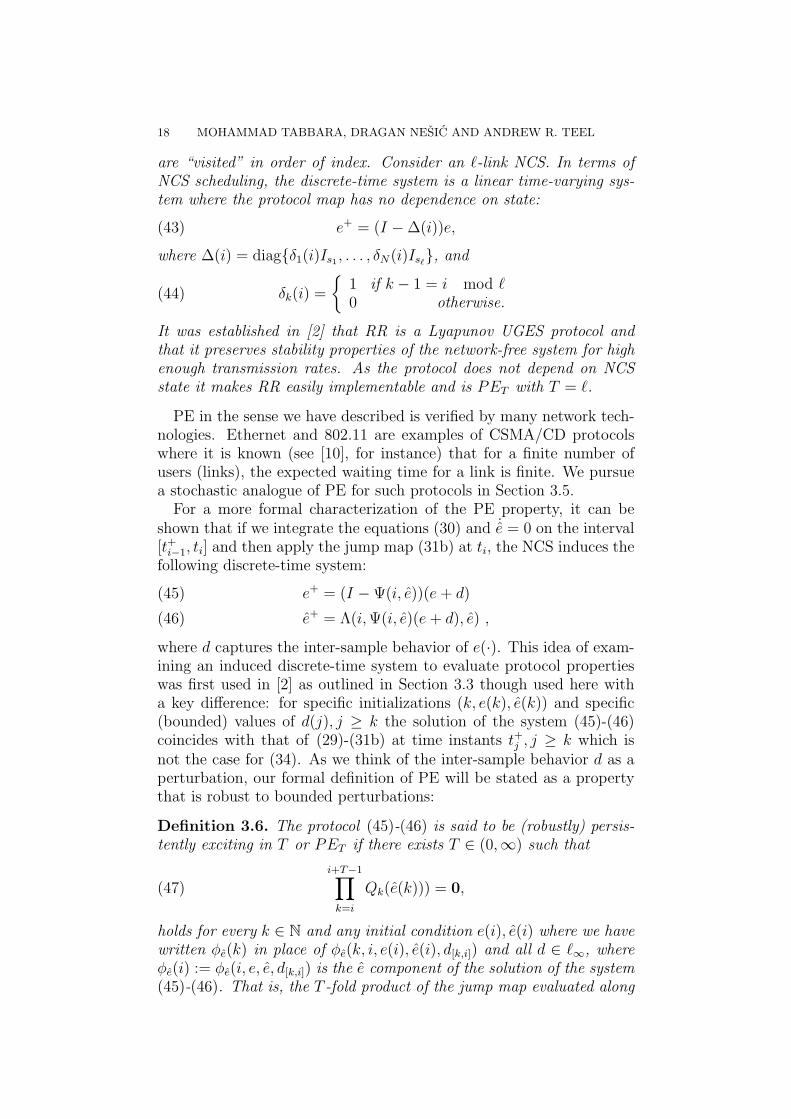
are “visited” in order of index. Consider an `-link NCS. In terms ofNCS scheduling, the discrete-time system is a linear time-varying sys-tem where the protocol map has no dependence on state:
(43) e+ = (I −∆(i))e,
where ∆(i) = diagδ1(i)Is1 , . . . , δN(i)Is`, and
(44) δk(i) =
1 if k − 1 = i mod `0 otherwise.
It was established in [2] that RR is a Lyapunov UGES protocol andthat it preserves stability properties of the network-free system for highenough transmission rates. As the protocol does not depend on NCSstate it makes RR easily implementable and is PET with T = `.
PE in the sense we have described is verified by many network tech-nologies. Ethernet and 802.11 are examples of CSMA/CD protocolswhere it is known (see [10], for instance) that for a finite number ofusers (links), the expected waiting time for a link is finite. We pursuea stochastic analogue of PE for such protocols in Section 3.5.
For a more formal characterization of the PE property, it can beshown that if we integrate the equations (30) and ˙e = 0 on the interval[t+i−1, ti] and then apply the jump map (31b) at ti, the NCS induces thefollowing discrete-time system:
e+ = (I −Ψ(i, e))(e+ d)(45)
e+ = Λ(i,Ψ(i, e)(e+ d), e) ,(46)
where d captures the inter-sample behavior of e(·). This idea of exam-ining an induced discrete-time system to evaluate protocol propertieswas first used in [2] as outlined in Section 3.3 though used here witha key difference: for specific initializations (k, e(k), e(k)) and specific(bounded) values of d(j), j ≥ k the solution of the system (45)-(46)coincides with that of (29)-(31b) at time instants t+j , j ≥ k which isnot the case for (34). As we think of the inter-sample behavior d as aperturbation, our formal definition of PE will be stated as a propertythat is robust to bounded perturbations:
Definition 3.6. The protocol (45)-(46) is said to be (robustly) persis-tently exciting in T or PET if there exists T ∈ (0,∞) such that
(47)i+T−1∏
k=i
Qk(e(k))) = 0,
holds for every k ∈ N and any initial condition e(i), e(i) where we havewritten φe(k) in place of φe(k, i, e(i), e(i), d[k,i]) and all d ∈ `∞, whereφe(i) := φe(i, e, e, d[k,i]) is the e component of the solution of the system(45)-(46). That is, the T -fold product of the jump map evaluated along
NETWORKED CONTROL SYSTEMS: EMULATION-BASED DESIGN 19
any set of trajectories that can be generated by (45)-(46) from any setof initial condition is the zero matrix.
The protocols below are typical of what has been proposed in NCSliterature and what is used in practice. In what follows, we will alwaysassume an `-link NCS with the ith linking consisting of li nodes andan error vector ei. Two PET protocols are presented next though wenote that the simplest example of a PE protocol is RR (Example 3.5).
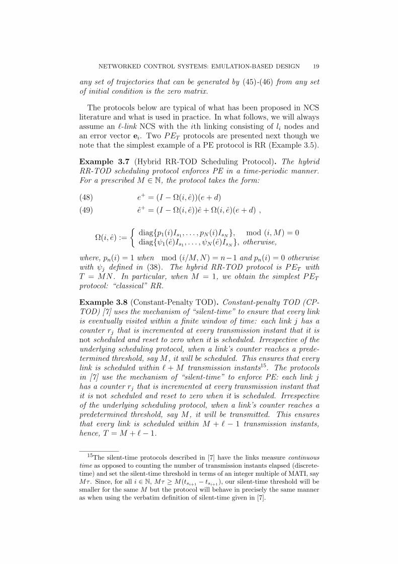
Example 3.7 (Hybrid RR-TOD Scheduling Protocol). The hybridRR-TOD scheduling protocol enforces PE in a time-periodic manner.For a prescribed M ∈ N, the protocol takes the form:
e+ = (I − Ω(i, e))(e+ d)(48)
e+ = (I − Ω(i, e))e+ Ω(i, e)(e+ d) ,(49)
Ω(i, e) :=
diagp1(i)Is1 , . . . , pN(i)IsN
, mod (i,M) = 0diagψ1(e)Is1 , . . . , ψN(e)IsN
, otherwise,
where, pn(i) = 1 when mod (i/M,N) = n−1 and pn(i) = 0 otherwisewith ψj defined in (38). The hybrid RR-TOD protocol is PET withT = MN . In particular, when M = 1, we obtain the simplest PET
protocol: “classical” RR.
Example 3.8 (Constant-Penalty TOD). Constant-penalty TOD (CP-TOD) [7] uses the mechanism of “silent-time” to ensure that every linkis eventually visited within a finite window of time: each link j has acounter rj that is incremented at every transmission instant that it isnot scheduled and reset to zero when it is scheduled. Irrespective of theunderlying scheduling protocol, when a link’s counter reaches a prede-termined threshold, say M , it will be scheduled. This ensures that everylink is scheduled within ` + M transmission instants15. The protocolsin [7] use the mechanism of “silent-time” to enforce PE: each link jhas a counter rj that is incremented at every transmission instant thatit is not scheduled and reset to zero when it is scheduled. Irrespectiveof the underlying scheduling protocol, when a link’s counter reaches apredetermined threshold, say M , it will be transmitted. This ensuresthat every link is scheduled within M + ` − 1 transmission instants,hence, T = M + `− 1.
15The silent-time protocols described in [7] have the links measure continuoustime as opposed to counting the number of transmission instants elapsed (discrete-time) and set the silent-time threshold in terms of an integer multiple of MATI, sayMτ . Since, for all i ∈ N, Mτ ≥ M(tsi+1 − tsi+1), our silent-time threshold will besmaller for the same M but the protocol will behave in precisely the same manneras when using the verbatim definition of silent-time given in [7].
20 MOHAMMAD TABBARA, DRAGAN NESIC AND ANDREW R. TEEL
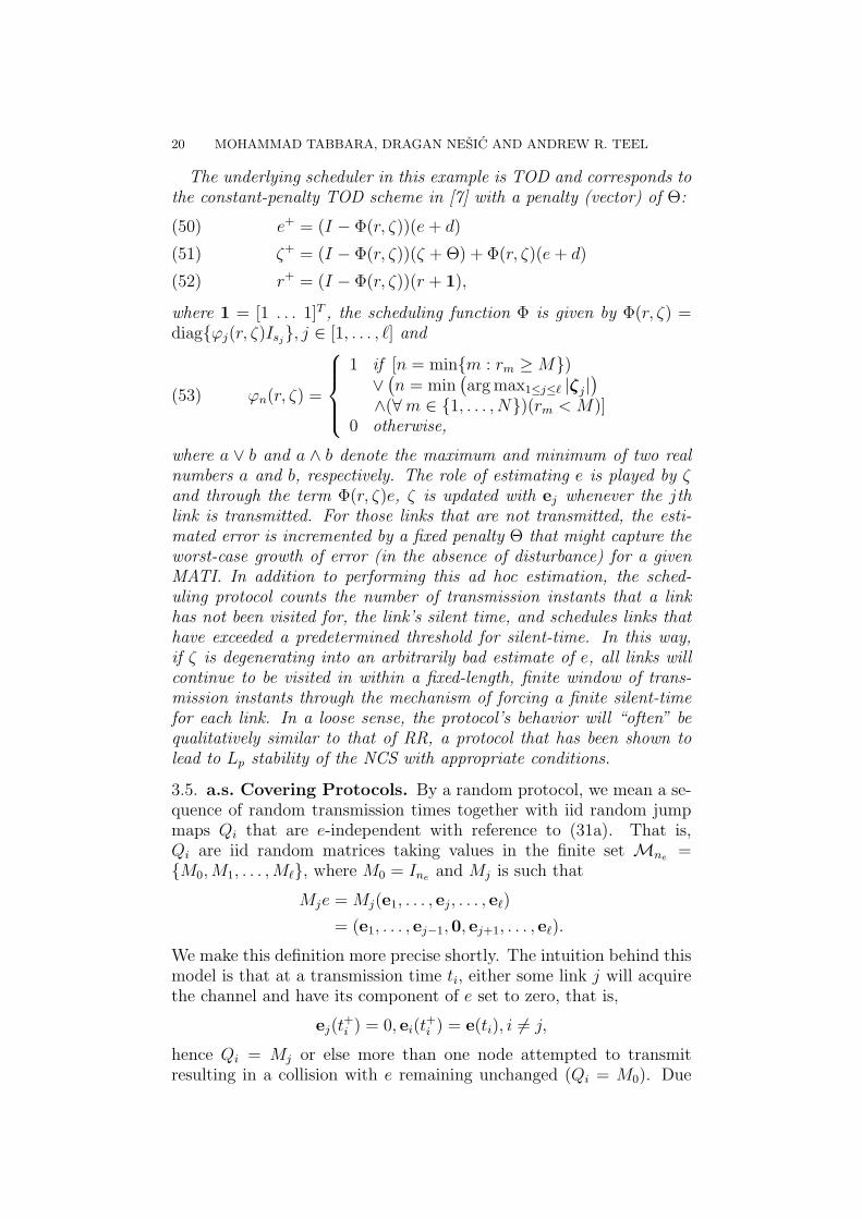
The underlying scheduler in this example is TOD and corresponds tothe constant-penalty TOD scheme in [7] with a penalty (vector) of Θ:
e+ = (I − Φ(r, ζ))(e+ d)(50)
ζ+ = (I − Φ(r, ζ))(ζ + Θ) + Φ(r, ζ)(e+ d)(51)
r+ = (I − Φ(r, ζ))(r + 1),(52)
where 1 = [1 . . . 1]T , the scheduling function Φ is given by Φ(r, ζ) =diagϕj(r, ζ)Isj
, j ∈ [1, . . . , `] and
(53) ϕn(r, ζ) =
1 if [n = minm : rm ≥M)∨(n = min
(arg max1≤j≤` |ζj|
)∧(∀m ∈ 1, . . . , N)(rm < M)]
0 otherwise,
where a ∨ b and a ∧ b denote the maximum and minimum of two realnumbers a and b, respectively. The role of estimating e is played by ζand through the term Φ(r, ζ)e, ζ is updated with ej whenever the jthlink is transmitted. For those links that are not transmitted, the esti-mated error is incremented by a fixed penalty Θ that might capture theworst-case growth of error (in the absence of disturbance) for a givenMATI. In addition to performing this ad hoc estimation, the sched-uling protocol counts the number of transmission instants that a linkhas not been visited for, the link’s silent time, and schedules links thathave exceeded a predetermined threshold for silent-time. In this way,if ζ is degenerating into an arbitrarily bad estimate of e, all links willcontinue to be visited in within a fixed-length, finite window of trans-mission instants through the mechanism of forcing a finite silent-timefor each link. In a loose sense, the protocol’s behavior will “often” bequalitatively similar to that of RR, a protocol that has been shown tolead to Lp stability of the NCS with appropriate conditions.
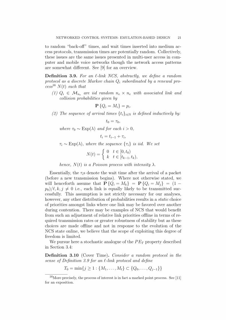
3.5. a.s. Covering Protocols. By a random protocol, we mean a se-quence of random transmission times together with iid random jumpmaps Qi that are e-independent with reference to (31a). That is,Qi are iid random matrices taking values in the finite set Mne =M0,M1, . . . ,M`, where M0 = Ine and Mj is such that
Mje = Mj(e1, . . . , ej, . . . , e`)
= (e1, . . . , ej−1,0, ej+1, . . . , e`).
We make this definition more precise shortly. The intuition behind thismodel is that at a transmission time ti, either some link j will acquirethe channel and have its component of e set to zero, that is,
ej(t+i ) = 0, ei(t
+i ) = e(ti), i 6= j,
hence Qi = Mj or else more than one node attempted to transmitresulting in a collision with e remaining unchanged (Qi = M0). Due
NETWORKED CONTROL SYSTEMS: EMULATION-BASED DESIGN 21
to random “back-off” times, and wait times inserted into medium ac-cess protocols, transmission times are potentially random. Collectively,these issues are the same issues presented in multi-user access in com-puter and mobile voice networks though the network access patternsare somewhat different. See [9] for an overview.
Definition 3.9. For an `-link NCS, abstractly, we define a randomprotocol as a discrete Markov chain Qi subordinated by a renewal pro-cess16 N(t) such that
(1) Qi ∈ Mne are iid random ne × ne with associated link andcollision probabilities given by
P Qi = Mi = pi.
(2) The sequence of arrival times tii∈N is defined inductively by:
t0 = τ0,
where τ0 ∼ Exp(λ) and for each i > 0,
ti = ti−1 + τi,
τi ∼ Exp(λ), where the sequence τi is iid. We set
N(t) =
0 t ∈ [0, t0)k t ∈ [tk−1, tk),
hence, N(t) is a Poisson process with intensity λ.
Essentially, the τis denote the wait time after the arrival of a packet(before a new transmission begins). Where not otherwise stated, wewill henceforth assume that P Qi = Mk = P Qi = Mj = (1 −p0)/`, k, j 6= 0 i.e., each link is equally likely to be transmitted suc-cessfully. This assumption is not strictly necessary for our analyses,however, any other distribution of probabilities results in a static choiceof priorities amongst links where one link may be favored over anotherduring contention. There may be examples of NCS that would benefitfrom such an adjustment of relative link priorities offline in terms of re-quired transmission rates or greater robustness of stability but as thesechoices are made offline and not in response to the evolution of theNCS state online, we believe that the scope of exploiting this degree offreedom is limited.
We pursue here a stochastic analogue of the PET property describedin Section 3.4:
Definition 3.10 (Cover Time). Consider a random protocol in thesense of Definition 3.9 for an `-link protocol and define
T0 = minj ≥ 1 : M1, . . . ,M` ⊂ Q0, . . . , Qj−1
16More precisely, the process of interest is in fact a marked point process. See [11]for an exposition.
22 MOHAMMAD TABBARA, DRAGAN NESIC AND ANDREW R. TEEL
and, inductively for i > 0,
Ti = minj ≥ 0 : M1, . . . ,M` ⊂ QTi−1, . . . , QTi−1+j−1.
We refer to Ti as the ith cover time and, collectively the cover timeprocess. It is clear from our definition of Qi that Ti is a stationaryprocess.
Definition 3.11 (Covering sequence). Let τi = ti+1 − ti, as in Defini-tion 3.9, that is, τi are inter-arrival times. We say that
C(j, k) = (Qj, τj), . . . , (Qk, τk), k ≥ j
is a covering sequence iff M1, . . . ,M` ⊂ C(1)(j, k).17 It is easy to see
that cover times are simply the lengths of consecutive disjoint coveringsequences.
Remark 3. From our definition of random protocols, the distributionof Tn is given by the solution to the (weighted) coupon collectors prob-lem. When pi = pj, i, j 6= 0, we have the closed form expression forthe expectation:
(54) E[T ] = `H`/(1− p0),
where H` is the `th harmonic number and we have dropped the timeindex n since Tn is stationary. We also have the bound for the distri-bution, P Tn ≥ β` ln `/(1− p0) ≤ `−(β−1)/(1 − p0), for any β > 1.Intuitively, Tn = E[T ] “most of the time” and P Tn <∞ = 1. /
Our abstract definition of a contention protocol is a model for thecontention protocols discussed earlier and to that end we present twonatural examples in this setting.
Definition 3.12 (Almost Surely Finite Cover Time). We say that aprotocol is a.s. covering or has an a.s. finite cover time if in Definition3.10
(∀i ∈ N) P Ti <∞ = 1.
Note that from the preceding discussion, this property is verified by allcontention protocols in the sense of Definition 3.9.
3.6. Slotted p-Persistent CSMA. What has been referred to as“scheduling” and the associated scheduling protocols by [12] is gen-erally known as medium access in the communications literature. Car-rier sense multiple access with collision detection (CSMA/CD) is byfar the most widely used medium access protocol by virtue of the sheervolume of Ethernet and Ethernet-like networking devices shipped andmanufactured each year.
CSMA/CD is a simple protocol: Links listen for transmissions onthe channel. A link wanting to transmit acquires the channel when
17The notation C(1)(j, k) refers to the covering sequence of matrices Qi with noreference to inter-transmission times τi i.e., Qj , . . . , Qk.
NETWORKED CONTROL SYSTEMS: EMULATION-BASED DESIGN 23
it senses that the channel is idle. When more than one link sensesthat the channel is idle and begins transmission, a collision occurs.At this point, all transmissions are immediately aborted. There areseveral variants of CSMA/CD that prescribe how transmissions arerescheduled and how links initially acquire the channel.
With slotted p-persistent CSMA, rather than have links transmitwhenever the channel is idle, links are only permitted to transmit atprescribed transmission slots that occur every ts > 0 seconds in slottedprotocols. At the start of slot sk, links S = i, .., j intending totransmit acquire the channel with a probability of p. If a collisionoccurs, links Sc are permitted to transmit in the next slot and links Sc
reschedule their transmissions at slots sk+di, . . . , sk+dj
.As alluded to earlier, the primary reason that CSMA protocols and,
indeed, all contention protocols work in practice is that the access pat-terns of computer and voice networks are “bursty” in nature. The as-sumption is that a link will occasionally transmit a burst of informationand remain otherwise idle. Transmissions are expected to eventuallysucceed as links are “infrequently” contending for the channel.
The situation is quite different for control networks with the impli-cation that medium access patterns are constant rather than burstyand for slotted p-persistent CSMA, we assume that every slot will bein contention. Another key difference between computer networks andNCS is in the treatment of collisions and dropouts. NCS should notbuffer failed transmissions of controller or sensor values but, rather,attempt to transmit the latest values when a slot is free. As the maxi-mum number of links contending slots is constant for every slot, thereis no reason for a link to delay transmission for any more than one slotafter a collision.
With these assumptions, consider an `-link NCS with the p-persistentCSMA protocol. The probability P Qi = Mj that a particular link jtransmits successfully during the ith slot is given by
P Qi = Mj = p(1− p)`−1.
It is clear that P Qi = Mj is maximized when p = 1/`. We willhenceforth set p = 1/` and have that
P Qi = Mj =1
`
(1− 1
`
)`−1
=(`− 1)`−1
``.
Notice that in this “optimal” case, P Qi = Mj = P Qi = Mk =(` − 1)`−1/`` for i, k 6= 0 and the probability of a collision is given byP Qi = M0 = 1− (`−1)`−1/``−1. Finally, we assume that slots occurevery ts > 0 seconds and, hence, p-persistent CSMA is a contentionprotocol in the sense of Definition 3.9 where inter-arrival times τi aredeterministic.
24 MOHAMMAD TABBARA, DRAGAN NESIC AND ANDREW R. TEEL
3.7. CSMA with Random Waits. Whereas the use of fixed slotstends to improve throughput and reduce collisions with computer net-works e.g., slotted versus pure ALOHA, the contention by every linkat every slot forces transmissions to happen in lock-step with NCSnetwork access patterns with the potential for a collision at every slot.
Suppose that instead of immediately acquiring the channel withprobability p after sensing the channel to be idle or after a new slotarrives, links instead wait a random amount of time before transmit-ting. In particular, if a particular link j waits for a random timeη′j ∼ Exp(λ/`) then, P Qi = Mj = (1−p0)/`, j 6= 0. The actual waittime before any particular transmission will be given
τ = minη′1, . . . , η′`;that is, the link that waits the least gets to transmit first, hence,τ ∼ Exp(λ). Assuming the wait times are iid for each link, thisis the prototypical example of what we mean by a stochastic protocoland a stochastic channel.
In the presence of transmission errors, p0 is generally nonzero and,conceptually, p-persistent CSMA and CSMA with random waits areessentially the same save for the fact that the transmission process istruly random with the latter. While CSMA with random waits can bethought of as a protocol in its own right when the random waits areenforced explicitly in the implementation, it can also be thought of asa model of medium access with NCS access patterns while using a classof CSMA wireless protocols. Delays in signal detection, multi-path ef-fects and varying processor loads mean that links are only prepared totransmit after some delay upon sensing the channel being idle and al-though the cumulative effects of these delays may not be exponentiallydistributed, the principle remains the same.
4. NCS Stability
The notion of robustness of various stability properties plays a funda-mental role in practical design and implementation of control systemsas evidenced by the extensive literature discussing, for example, input-to-state stability (ISS), H2, H∞ design and variants of robust stability.To that end, [2] and [6] have examined Lp and input-to-state stabilityof NCS, respectively and it was shown in [12] that persistently excitingscheduling protocols lead to Lp stable NCS when appropriate conditionsare imposed on transmission rates and the nominal system and similarresults were provided for UGES and UGAS protocols in [2] and [6],respectively. While the proof techniques and settings are substantiallydifferent, the novel use of various small-gain theorems is a unifyingtheme throughout these results and a powerful tool for quantifying ro-bustness. See [13, Chapter 5.4] for an introduction to the notion ofinput/output stability gain and [14] for general ISS small-gain results.
NETWORKED CONTROL SYSTEMS: EMULATION-BASED DESIGN 25
We outline several NCS stability results in the ensuing sections andrefer to the reader to [2], [6] and [12] for where the results are stated andproved in greater generality. Finally, while these results are ISS/IOStype results, whenever exogeneous perturbations are removed, UGESand UGAS can be recovered under additional mild technical assump-tions. See [2, Section II-B], for instance.
We first recall the definition of Lp stability and detectability for asystem Σz with jumps:
(55) Σz : z = f(t, z, w) t ∈ [ti, ti+1] ,
output y(t) = g(t, z) and with jump equation
(56) z(t+i ) = h(i, z(ti)),
Let f : R → Rn be a (Lebesgue) measurable function and de-
fine ‖f‖p :=(∫
R |f(s)|pds)1/p
for 1 ≤ p < ∞ and define ‖f‖∞ :=ess. supt∈R |f(t)|. We say that f ∈ Lp for p ∈ [1,∞] whenever ‖f‖p <∞. Let f : R→ Rn and let [a, b] ⊂ R. We use the notation
‖f [a, b]‖p :=
(∫[a,b]
|f(s)|pds)1/p
to denote the Lp norm of f when restricted to the interval [a, b].
Definition 4.1. Let p ∈ [1,∞] and γ ≥ 0 be given. We say thatΣz is Lp stable from w to y with gain γ if ∃ K ≥ 0 : ‖y[t0, t]‖p ≤K|z0|+ γ‖w[t0, t]‖p.Definition 4.2. Let p, q ∈ [1,∞] and γ ≥ 0 be given. The state zof Σz is said to be Lp to Lq detectable from output y with gain γ if∃K ≥ 0 : ‖z[t0, t]‖q ≤ K|z0|+ γ‖y[t0, t]‖p + γ‖w[t0, t]‖p.
An exposition of these ideas as they pertain to NCS can be foundin [2, Section II-B].
4.1. Lp Stability of NCS with Lyapunov UGES Protocols. Amore general version of the following result was first presented in [2] andasserts that Lyapunov UGES scheduling protocols preserve Lp stabilityof the network-free system under appropriate conditions and for smallenough values of MATI.
Theorem 4.3. Consider NCS (29)-(31b) and suppose that:
(i) That the NCS scheduling protocol (31a) is Lyapunov UGES withLyapunov function W that is locally Lipschitz in e, uniformly ini and there exists L ≥ 0 such that:
(57)
⟨∂W (i, e)
∂e, g(t, x, e, w)
⟩≤ LW (i, e) + |y|,
for almost all e ∈ Rne, for all (x,w) ∈ Rnx×Rnw , all t ∈ (ti, ti+1),for all i ∈ N, where y : Rne × Rnw → R is a continuous functionof (x,w);
26 MOHAMMAD TABBARA, DRAGAN NESIC AND ANDREW R. TEEL
(ii) system (29) is Lp stable from (W,w) to y with gain γ for somep ∈ [1,∞]; (x,w) is Lp to Lp detectable from y; (e, w) is Lp to Lp
detectable from W ;(iii) and MATI satisfies τ ∈ (ε, τ ∗), ε ∈ (0, τ ∗), where
(58) τ ∗ =1
Lln
(L+ γ
θL+ γ
),
where θ comes from (41).
Then, the NCS is Lp-stable from w to (x, e) with linear gain.
Remark 4. Within the framework of hybrid systems presented in [15],results analogous to Theorem 4.3 are developed in [16] where τ ∗ is givenby
τ ∗ =
1
Lrarctan
(r(1− θ)
2 θ1+θ
(γL− 1)
+ 1 + θ
)γ > L
1
L
1− θ1 + θ
γ = L
1
Lrarctanh
(r(1− θ)
2 θ1+θ
(γL− 1)
+ 1 + θ
)γ < L ,
(59)
where
(60) r =
√∣∣∣∣(γL)2
− 1
∣∣∣∣ .This bound is shown improve upon (58) in [16] when verifying UGES,the results therein are stated for UGAS, UGES and semi-global practicalISS and can, in principle, be extended to apply to Lp IOS.
4.2. Lp Stability of NCS with PET Protocols. The following the-orem asserts that PE protocols lead to Lp stability of the NCS forsufficiently small MATI. While we do not provide a closed-form ex-pression for MATI bounds, the bounds are readily obtained in exam-ples by numerically solving for τ ∗ in (62). Note that we only considerstability of e and x. The decision-vector, if used in the protocol beinganalyzed, may fail to verify any stability properties but as e has nophysical significance as a state vector whose evolution is governed bythe protocol, this is generally not an issue. Let An denote the set ofall n×n matrices and let A+
n denote the subset of all matrices that arepositive semi-definite, symmetric and have positive entries and let Rn
+
denote the nonnegative orthant.
Theorem 4.4. Consider NCS (29)-(31b) and suppose that:
(i) The NCS scheduling protocol (31b) is uniformly persistently ex-citing in time T and there exists A ∈ A+
neand a continuous
NETWORKED CONTROL SYSTEMS: EMULATION-BASED DESIGN 27
y : Rnx × Rnw → Rne+ so that the error dynamics (30) satisfy18
(61) g(t, x, e, w) Ae+ y(x,w)
for all (x, e, w) ∈ Rnx ×Rne ×Rnw , all t ∈ (ti, ti+1), for all i ∈ N.hold with y = G(x) +H(w);
(ii) system (29) is Lp stable from (e, w) to G(x) with gain γ for somep ∈ [1,∞]; (x,w) is Lp to Lp detectable from y;
(iii) and MATI satisfies τ ∈ (ε, τ ∗), ε ∈ (0, τ ∗), where τ ∗ = ln(z)|A|T and z
solves
(62) γκTz1+1/T + z(|A| − γκT )− 2|A| = 0,
where κ = exp(−1) and |A| comes from (61).
Then, the NCS is Lp-stable from w to (x, e) with linear gain.
Remark 5. Suppose that g(t, x, e, w) = Bx+Ce+Dw and let A = [aij],where aij = max|cij|, |cji| and y(x,w) = Bx+Dw. We immedi-ately have that A and y(x,w) satisfy condition 2 of Theorem 4.4 and‖y(x,w)‖p = ‖Bx +Dw‖p ≤ ‖Bx‖p + ‖Dw‖p. Whenever g satisfies alinear growth bound of the form |g(t, x, e, w)| ≤ L(|x|+ |e|+ |w|), it isstraightforward to construct an appropriate A and y. /
Remark 6. Suppose that the network-free system is Lp stable fromw to x with gain γ and the NCS satisfies the hypotheses of Theorem4.4. Then for any γ∗ > γ, it is possible to show that there exists aMATI τ such that the NCS is Lp stable from w to x with gain γ∗.This corollary of Theorem 4.4 is particularly useful in the design ofoptimal/robust controllers. /
4.3. Lp stability of NCS with Random Protocols. This followingresult analyzes the input-output Lp stability (IOS) of NCS (in expecta-tion), the essence of which is that outputs (or state) of an NCS verify arobustness property with respect to exogenous disturbances. We stressthat it is only the network protocol and channel that induces random-ness in our models and that the exogenous disturbances are Lp signalsas in [2] and [12].
Although link cover times and inter-transmission are now randomand, hence, not uniform, if the network-free system is Lp stable, theNCS remains so with any contention protocol, in the sense of our def-inition, whenever attempted transmissions occur “fast enough”. By“fast enough” we mean that there exists a choice of intensity λ of thetransmission process parameterized by properties of the protocol and
18Let x = (x1, . . . , xn), y = (y1, . . . , yn) ∈ Rn. The vector partial order isgiven by x y ⇐⇒ (x1 ≤ y1) ∧ · · · ∧ (xn ≤ yn) and e and g are given by
e := (|e1|, . . . , |ene|)T and t
g7→ g(t), respectively. That is, e is the vector thatresults from taking the absolute value of each scalar component of e and g doesoperates analogously on the image of g.
28 MOHAMMAD TABBARA, DRAGAN NESIC AND ANDREW R. TEEL
the NCS dynamics such that the NCS is Lp stable-in-expectation fromdisturbance to NCS state with a finite expected gain.
Intuitively, and despite the presence of collisions, random packetdropouts and random inter-arrival times, it seems natural to expectthat the stability of the NCS (24)-(28a) for high enough “average”transmission rates and in light of the a.s. cover times of contentionprotocols and in analogy with persistently exciting scheduling proto-cols, this stability ought to be robust in an Lp sense. In fact, if werelax our notion of “Lp stability” to “Lp stability-in-expectation”, wecan prove a positive result in that direction. The definition of theseproperties is obtained, essentially, by using expected norms E‖ · ‖ inlieu of ‖ · ‖ in Definition 4.1 and Definition 4.2. We stress that, asdeveloped in this chapter, these notions only apply to hybrid systemsof the form (55)-(56), i.e., we insist that w is “essentially” an Lp signaland not a Levy process (c.f. [17]) specifically because we are concernedwith robustness of stability in the sense of e.g., [18], whereas a Levyprocess characterization of disturbances may be more appropriate inmodeling sensor noise and quantization phenomena.
While the following results are stated for the delay and inter-arrivalprocesses presented in Definition 3.9, it is straightforward to extendthem to a more general class of processes.
Theorem 4.5. Consider an `-link NCS (29)-(31b) and suppose that:
(i) the NCS employs a contention scheduling protocol with iid covertimes Ti and the inter-arrival process is Poisson with intensity λand also suppose that the NCS error dynamics satisfy
(63) g(t, x, e, w) Ae+ y(x,w)
for all (x, e, w) ∈ Rnx × Rne × Rnw and almost all t, where A isa nonnegative symmetric ne×ne matrix with nonnegative entriesand y = G(x) +H(w);
(ii) system (29) is Lp stable-in-expectation from (e, w) to G(x) withexpected gain γ for some p ∈ [1,∞]; (30) is Lp to Lp detectable-in-expectation from y;
Then, there exists λ < ∞ depending on (`, |A|, γ,E[T ], p0) such thatthe NCS is Lp stable-in-expectation from w to (x, e) with a finite linearexpected gain 1/(1− γγ∗). Specifically, λ solves γ∗γ < 1 with
γ∗ =E[T ](1 + ρ)
(λ− |A|)(1− ρ),
where,
ρ = (α(1− p0))`∏k=1
`− (k − 1)
`(1− p0α)− (k − 1)(1− p0)α− 1,
and α =(
λλ−|A|
)and λ > |A|
1−p0.
NETWORKED CONTROL SYSTEMS: EMULATION-BASED DESIGN 29
Remark 7. While no bounds for λ are given, the requisite intensitycan be found numerically. /
4.4. Lp stability of NCS with a.s. Lyapunov Protocols. Thefollowing result is a natural extension to Theorem 4.3 for channels thathave a non-zero probability of packet dropout and is intended to beused in much the same way as the latter result. While [2] presentssufficient conditions for Lp stability in the presence of deterministicallycharacterized packet dropouts for Lyapunov UGES protocols, we be-lieve the following result is a more natural treatment of dropouts andthe conditions are directly verifiable.
Theorem 4.6. Consider NCS (29)-(31b) and suppose that:
(i) The NCS scheduling protocol (31a) is a.e. Lyapunov UGES withLyapunov function W that is locally Lipschitz in e, uniformly ini and there exists L ≥ 0 such that:
(64)
⟨∂W (i, e)
∂e, g(t, x, e, w)
⟩≤ LW (i, e) + |y|,
for almost all e ∈ Rne, for all (x,w) ∈ Rnx×Rnw , all t ∈ (ti, ti+1),for all i ∈ N, where y : Rne × Rnw → R is a continuous functionof (x,w);
(ii) system (29) is Lp stable from (W,w) to y with finite expected gainγ for some p ∈ [1,∞]; (x,w) is Lp to Lp detectable from y withfinite expected gain; e is Lp detectable from W with finite expectedgain;
(iii) the channel packet dropout probability is given by p0 ≥ 0 and (36)is satisfied with an iid sequence κi such that the intensity of theinter-transmission process λ satisfies
(65) λ >γ + L
1− E[κ].
Then, the NCS is Lp-stable from w to (x, e) with finite expected lineargain:
(66)λ(1− E[κ])− L
λ(1− E[κ])− L− γ.
Remark 8. As the motivation for studying a.s. Lyapunov UGEScomes from the use of Lyapunov UGES protocols on non-ideal chan-nels, we can restate several of the conditions of Theorem 4.6 in lightof Proposition 3.4. Let θ be as in (41) and let the probability of packetdropout p0 satisfy (42). The requisite intensity in (65) becomes
(67) λ >γ + L
(1− p0)(1− θ)and the resultant gain (66) can be re-expressed in a similar manner.
30 MOHAMMAD TABBARA, DRAGAN NESIC AND ANDREW R. TEEL
Remark 9. As in [2] and [12], in both this and the preceding section,several generalizations and specializations of the stability results arepossible. With additional technical assumptions on the NCS dynamics,one can conclude uniform global exponential stability (in expectation)and the assumptions on the various reset maps can be relaxed so asto infer ISS-like properties in lieu of Lp stability as discussed [6]. Ifwe forgo the detectability assumptions in the hypotheses of Theorem4.5 and Theorem 4.6 we can only infer input-to-output stability-in-expectation. /
5. Case Studies & Comparisons
The aim of this section is to examine the various results presentedin this chapter and compare and contrast them to results presented inthe literature. For simplicity will focus on the following linear time-invariant systems where the simplified equations for an `-link NCS aregiven by (6) together with jump equations (31a) or (31b):
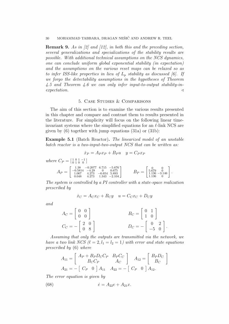
Example 5.1 (Batch Reactor). The linearized model of an unstablebatch reactor is a two-input-two-output NCS that can be written as:
xP = APxP +BPu y = CPxP
where CP = [ 1 0 1 −10 1 0 0 ]
AP =
[1.38 −0.2077 6.715 −5.676
−0.5814 −4.29 0 0.6751.067 4.273 −6.654 5.8930.048 4.273 1.343 −2.104
]BP =
[0 0
5.679 01.136 −3.1461.136 0
].
The system is controlled by a PI controller with a state-space realizationprescribed by
xC = ACxC +BCy u = CCxC +DCy
and
AC =
[0 00 0
]BC =
[0 11 0
]CC = −
[2 00 8
]DC = −
[0 2−5 0
].
Assuming that only the outputs are transmitted via the network, wehave a two link NCS (` = 2, l1 = l2 = 1) with error and state equationsprescribed by (6) where
A11 =
[AP +BPDCCP BPCC
BCCP AC
]A12 =
[BPDC
BC
]A21 = −
[CP 0
]A11 A22 = −
[CP 0
]A12.
The error equation is given by
(68) e = A22e+ A21x.
NETWORKED CONTROL SYSTEMS: EMULATION-BASED DESIGN 31
This example is used as the benchmark in comparing the inter-transmission bounds with the stability analysis frameworks outlinedin this chapter and in [4, 5, 7].
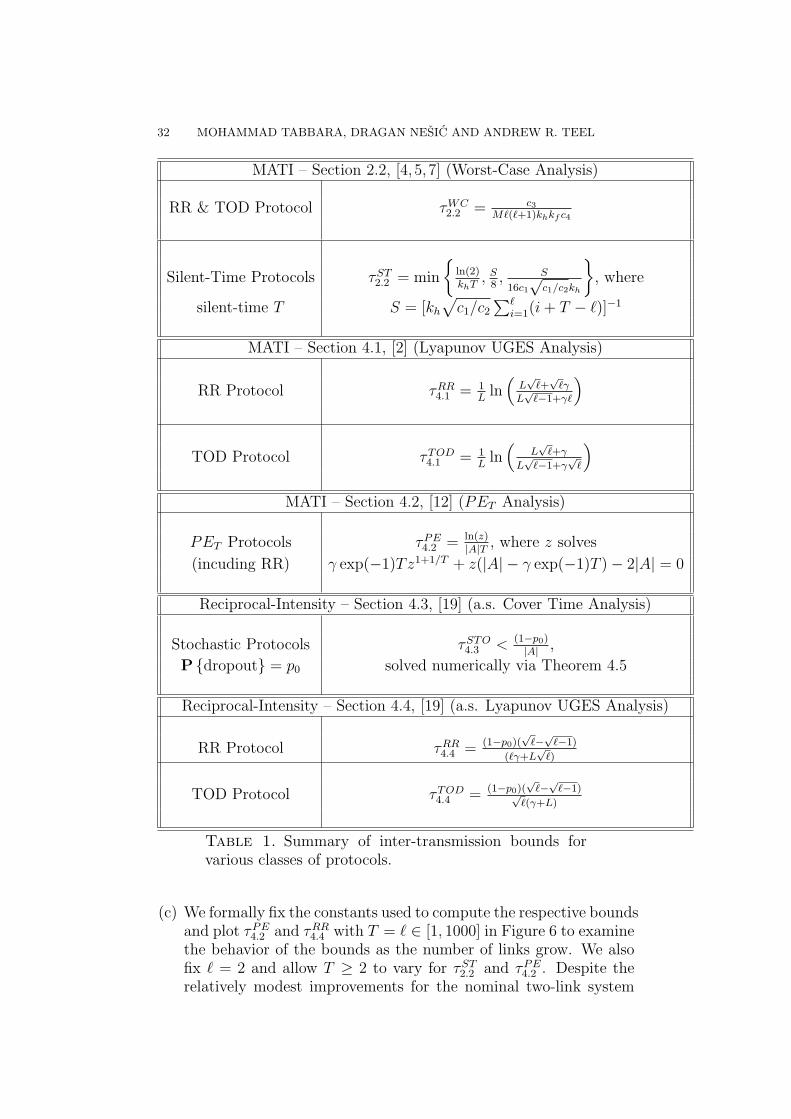
5.1. Analytical Inter-transmission Bounds Comparison. Priorto making numerical comparisons with respect to the bounds obtainedfor Example 5.1, we provide a brief summary of the analytical boundsin Table 1 as they apply in general. The various constants used aredefined and explained in the respective referenced sections and detailscan be found in the respective sources cited in the table. These arebounds at the boundary of stability. For all bounds presented, stabilityis in the sense of Lp (in-expectation) except for those derived in [4,5,7],where UGES is the applicable notion of stability.
Table 2 compares a selection of these MATI bounds as they apply toTOD and RR. It is shown in [12][Section VI-C] that for LTI systemsemploying RR scheduling, MATI bounds obtained within the frame-work outlined in Section 4.2 are asymptotically larger by a factor ofO(`1/2) than the MATI obtained in [2] which are, in turn, shown tobe analytically superior to the bounds in [3] for both TOD and RR.As indicated in Remark 4, for protocols that are Lyapunov UGES orUGAS, [16] may offer improved MATI bounds over [2] and, for thebatch reactor example, these were demonstrated to be an improvementof approximately 10%.
5.2. Numerical Inter-transmission Bounds Comparison (p0 =0). For simplicity, and since Lp stability results are not provided in [7],we will largely restrict our discussion absence of exogenous disturbancesand examine bounds that verify UGES and related properties. Much ofthe focus will be on RR scheduling as it is the only scheduling protocolthat can been mutually treated by the analysis frameworks in thischapter, [2] and [7] but several other protocols will be examined aswell.
We present and compare various results for the batch reactor exam-ple, Example 5.1, following [2], [3] and [12]. The comparison resultsare summarized below:
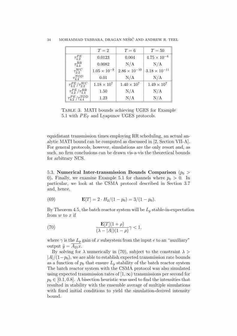
(a) The MATI bounds are shown in Table 3 with the bounds computedvia the PE framework larger than those obtained using the resultsof [7] by a factor of 107 and larger than the bound obtained by theresults of [2] by factor of 1.5. The bounds τPE
4.2 and τWC2.2 apply to
any PET protocol for the original two-link system. The bound τRR4.1
only applies to RR (T = ` = 2).(b) When using RR, τPE
4.2 that achieves UGES is equivalent to a networkthroughput of 84 kbps (assuming 128 byte frames), achievable oncurrent 802.11g and 802.11b wireless networks and τRR
4.4 requires aneffective network throughput of approximately 125 kbps.
32 MOHAMMAD TABBARA, DRAGAN NESIC AND ANDREW R. TEEL
MATI – Section 2.2, [4, 5, 7] (Worst-Case Analysis)
RR & TOD Protocol τWC2.2 = c3
M`(`+1)khkf c4
Silent-Time Protocols τST2.2 = min
ln(2)khT
, S8, S
16c1√
c1/c2kh
, where
silent-time T S = [kh
√c1/c2
∑`i=1(i+ T − `)]−1
MATI – Section 4.1, [2] (Lyapunov UGES Analysis)
RR Protocol τRR4.1 = 1
Lln(
L√
`+√
`γ
L√
`−1+γ`
)
TOD Protocol τTOD4.1 = 1
Lln(
L√
`+γ
L√
`−1+γ√
`
)MATI – Section 4.2, [12] (PET Analysis)
PET Protocols τPE4.2 = ln(z)
|A|T , where z solves
(incuding RR) γ exp(−1)Tz1+1/T + z(|A| − γ exp(−1)T )− 2|A| = 0
Reciprocal-Intensity – Section 4.3, [19] (a.s. Cover Time Analysis)
Stochastic Protocols τSTO4.3 < (1−p0)
|A| ,
P dropout = p0 solved numerically via Theorem 4.5
Reciprocal-Intensity – Section 4.4, [19] (a.s. Lyapunov UGES Analysis)
RR Protocol τRR4.4 = (1−p0)(
√`−√
`−1)
(`γ+L√
`)
TOD Protocol τTOD4.4 = (1−p0)(
√`−√
`−1)√`(γ+L)
Table 1. Summary of inter-transmission bounds forvarious classes of protocols.
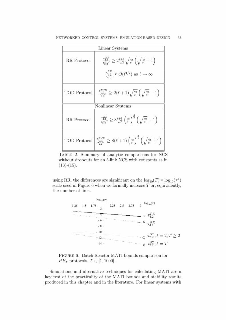
(c) We formally fix the constants used to compute the respective boundsand plot τPE
4.2 and τRR4.4 with T = ` ∈ [1, 1000] in Figure 6 to examine
the behavior of the bounds as the number of links grow. We alsofix ` = 2 and allow T ≥ 2 to vary for τST
2.2 and τPE4.2 . Despite the
relatively modest improvements for the nominal two-link system
NETWORKED CONTROL SYSTEMS: EMULATION-BASED DESIGN 33
Linear Systems
RR ProtocolτRR4.1
τWC2.2≥ 2 `+1√
`
√c2c1
(√c2c1
+ 1)
τPE4.2
τRR4.1≥ O(`1/2) as `→∞
TOD ProtocolτTOD4.1
τWC2.2≥ 2(`+ 1)
√c2c1
(√c2c1
+ 1)
Nonlinear Systems
RR ProtocolτRR4.1
τWC2.2≥ 8 `+1√
`
(c2c1
) 32(√
c2c1
+ 1)
TOD ProtocolτTOD4.1
τWC2.2≥ 8(`+ 1)
(c2c1
) 32(√
c2c1
+ 1)
Table 2. Summary of analytic comparisons for NCSwithout dropouts for an `-link NCS with constants as in(13)-(15).
using RR, the differences are significant on the log10(T )× log10(τ∗)
scale used in Figure 6 when we formally increase T or, equivalently,the number of links.
Theorem 5.2 [1, Section III] T=N [2, Theorem 1] N=2, T ≥ 2 [2, Theorem 1] T=N
log10HTLlog10(t )*
1.25 1.5 1.75 2.25 2.5 2.75 3
- 14
- 12
- 10
- 8
- 6
- 4
- 2
τPE4.2
τRR4.1
τST2.2 , ` = 2, T ≥ 2
τST2.2 , ` = T
Figure 6. Batch Reactor MATI bounds comparison forPET protocols, T ∈ [1, 1000].
Simulations and alternative techniques for calculating MATI are akey test of the practicality of the MATI bounds and stability resultsproduced in this chapter and in the literature. For linear systems with
34 MOHAMMAD TABBARA, DRAGAN NESIC AND ANDREW R. TEEL
T = 2 T = 6 T = 50
τPE4.2 0.0123 0.004 4.75× 10⁻⁴
τRR4.4 0.0082 N/A N/A
τWC2.2 1.05× 10⁻⁹ 2.86× 10⁻¹⁰ 3.18× 10⁻¹¹
τTOD4.4 0.01 N/A N/A
τPE4.2 /τWC
2.2 1.18× 10⁷ 1.40× 10⁷ 1.49× 10⁷
τPE4.2 /τRR
4.4 1.50 N/A N/A
τPE4.2 /τTOD
4.4 1.23 N/A N/A
Table 3. MATI bounds achieving UGES for Example5.1 with PET and Lyapunov UGES protocols.
equidistant transmission times employing RR scheduling, an actual an-alytic MATI bound can be computed as discussed in [2, Section VII-A].For general protocols, however, simulations are the only resort and, assuch, no firm conclusions can be drawn vis-a-vis the theoretical boundsfor arbitrary NCS.
5.3. Numerical Inter-transmission Bounds Comparison (p0 >0). Finally, we examine Example 5.1 for channels where p0 > 0. Inparticular, we look at the CSMA protocol described in Section 3.7and, hence,
(69) E[T ] = 2 ·H2/(1− p0) = 3/(1− p0).
By Theorem 4.5, the batch reactor system will be Lp stable-in-expectationfrom w to x if
(70)E[T ](1 + ρ)
(λ− |A|)(1− ρ)γ < 1,
where γ is the Lp gain of x subsystem from the input e to an “auxiliary”output y = A21x.
By solving for λ numerically in (70), subject to the constraint λ >|A|/(1−p0), we are able to establish expected transmission rate boundsas a function of p0 that ensure Lp stability of the batch reactor systemThe batch reactor system with the CSMA protocol was also simulatedusing expected transmission rates of [1,∞) transmissions per second forp0 ∈ [0.1, 0.8]. A bisection heuristic was used to find the intensities thatresulted in stability with the ensemble average of multiple simulationswith fixed initial conditions to yield the simulation-derived intensitybound.
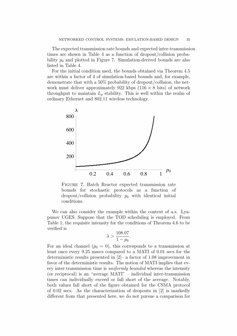
NETWORKED CONTROL SYSTEMS: EMULATION-BASED DESIGN 35
The expected transmission rate bounds and expected inter-transmissiontimes are shown in Table 4 as a function of dropout/collision proba-bility p0 and plotted in Figure 7. Simulation-derived bounds are alsolisted in Table 4.
For the initial condition used, the bounds obtained via Theorem 4.5are within a factor of 4 of simulation-based bounds and, for example,demonstrate that with a 50% probability of dropout/collision, the net-work must deliver approximately 922 kbps (116 × 8 bits) of networkthroughput to maintain Lp stability. This is well within the realm ofordinary Ethernet and 802.11 wireless technology.
0.2 0.4 0.6 0.8 1p0
200
400
600
800
lλ
Figure 7. Batch Reactor expected transmission ratebounds for stochastic protocols as a function ofdropout/collision probability p0 with identical initialconditions.
We can also consider the example within the context of a.s. Lya-punov UGES. Suppose that the TOD scheduling is employed. FromTable 1, the requisite intensity for the conditions of Theorem 4.6 to beverified is
λ >108.07
1− p0
.
For an ideal channel (p0 = 0), this corresponds to a transmission atleast once every 9.25 msecs compared to a MATI of 0.01 secs for thedeterministic results presented in [2]– a factor of 1.08 improvement infavor of the deterministic results. The notion of MATI implies that ev-ery inter-transmission time is uniformly bounded whereas the intensity(or reciprocal) is an “average MATI” – individual inter-transmissiontimes can individually exceed or fall short of the average. Notably,both values fall short of the figure obtained for the CSMA protocolof 0.02 secs. As the characterization of dropouts in [2] is markedlydifferent from that presented here, we do not pursue a comparison for
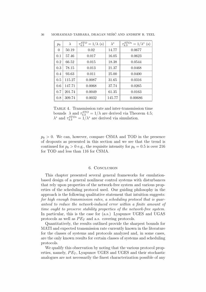
36 MOHAMMAD TABBARA, DRAGAN NESIC AND ANDREW R. TEEL
p0 λ τSTO4.3 = 1/λ (s) λ∗ τSTO∗
4.3 = 1/λ∗ (s)
0 50.19 0.02 14.77 0.0677
0.1 57.46 0.017 16.05 0.0623
0.2 66.52 0.015 18.38 0.0544
0.3 78.15 0.013 21.37 0.0468
0.4 93.63 0.011 25.00 0.0400
0.5 115.27 0.0087 31.65 0.0316
0.6 147.71 0.0068 37.74 0.0265
0.7 201.74 0.0049 61.35 0.0163
0.8 309.74 0.0032 145.77 0.00686
Table 4. Transmission rate and inter-transmission timebounds λ and τSTO
4.3 = 1/λ are derived via Theorem 4.5;λ∗ and τSTO∗
4.3 = 1/λ∗ are derived via simulation.
p0 > 0. We can, however, compare CSMA and TOD in the presenceof dropouts as presented in this section and we see that the trend iscontinued for p0 > 0 e.g., the requisite intensity for p0 = 0.5 is over 216for TOD and less than 116 for CSMA.
6. Conclusion
This chapter presented several general frameworks for emulation-based design of a general nonlinear control systems with disturbancesthat rely upon properties of the network-free system and various prop-erties of the scheduling protocol used. Our guiding philosophy in theapproach is the following qualitative statement that intuition suggests:for high enough transmission rates, a scheduling protocol that is guar-anteed to reduce the network-induced error within a finite amount oftime ought to preserve stability properties of the network-free system.In particular, this is the case for (a.s.) Lyapunov UGES and UGASprotocols as well as PET and a.s. covering protocols.
Quantitatively, the results outlined provide the sharpest bounds forMATI and expected transmission rate currently known in the literaturefor the classes of systems and protocols analyzed and, in some cases,are the only known results for certain classes of systems and schedulingprotocols.
We qualify this observation by noting that the various protocol prop-erties, namely, PET , Lyapunov UGES and UGES and their stochasticanalogues are not necessarily the finest characterization possible of any
NETWORKED CONTROL SYSTEMS: EMULATION-BASED DESIGN 37
particular protocol. This is reflected in the disparity between theoret-ical MATI and transmission rate values and those obtained by simu-lations. For example, it is known that for LTI systems employing RRwith equidistant inter-transmission times, analytic MATI bounds thatachieve UGES can be computed and, indeed, are as sharp or sharperthan those obtained by any result in this chapter. The aim of thischapter, however, was to present emulation-type results and designprocedures for the largest class of systems for which results are cur-rently known and which are useful in practice. To that end, we believethat this work serves as a useful starting point from which there is stillmuch scope for improvement.
References
[1] G. Walsh and H. Ye, “Scheduling of Networked Control Systems,” IEEE Con-trol Syst. Mag., vol. 21, no. 1, pp. 57–65, 2001.
[2] D. Nesic and A. Teel, “Input-output stability properties of networked controlsystems,” IEEE Trans. Automat. Contr., vol. 49, no. 10, pp. 1650–1667, 2004.
[3] G. Walsh, O. Beldiman, and L. Bushnell, “Asymptotic behaviour of nonlinearnetworked control systems,” IEEE Trans. Automat. Contr., vol. 46, no. 7, pp.1093–1097, 2001.
[4] W. Zhang, M. Branicky, and S. Phillips, “Stability of networked control sys-tems,” IEEE Control Syst. Mag., vol. 21, no. 1, pp. 84–99, 2001.
[5] G. Walsh, H.Ye, and L. Bushnell, “Stability analysis of networked controlsystems,” in American Control Conference, San Deigo, CA, Jun 1999.
[6] D. Nesic and A. Teel, “Input-to-state stability of networked control system,”Automatica, vol. 40, no. 12, pp. 2121–2128, 2004.
[7] H. Ye, G. Walsh, and L. Bushnell, “Real-time mixed-traffic wireless networks,”IEEE Trans. Ind. Electron., vol. 48, no. 5, pp. 883–890, 2001.
[8] M. Tabbara, D. Nesic, and A. Teel, “Input-output stability of wireless net-worked control systems,” in Proc. 44th IEEE Conf. on Dec. and Control, 2005.
[9] A. S. Tanenbaum, Computer Networks, 4th ed. Prentice Hall, 2003.[10] E. Coyle and B. Liu, “A Matrix Representation of CSMA/CD Networks,”
IEEE Trans. Commun., vol. 33, no. 1, pp. 53–64, Jan. 1985.[11] K. Sigman, Stationary marked point processes: an intuitive approach. Chap-
man & Hall, 1995.[12] M. Tabbara, D. Nesic, and A. Teel, “Stability of Wireless and Wireline Net-
worked Control Systems,” to appear in IEEE Trans. Automat. Contr., 2007.[13] H. Khalil, Nonlinear Systems, 3rd ed. Prentice Hall, 2002.[14] Z. Jiang, A. Teel, and L. Praly, “Small gain theorem for iss systems and ap-
plications,” Math. Contr. Sign. Syst., vol. 7, pp. 95–120, 1994.[15] R. Goebel and A. Teel, “Solutions to hybrid inclusions via set and graphical
convergence with stability theory applications,” Automatica, vol. 42, no. 4, pp.573–587, 2006.
[16] D. Carnevale, A. Teel, and D. Nesic, “A Lyapunov proof of an improved max-imum allowable transfer interval for networked control systems,” to appear inIEEE Trans. Automat. Contr., 2007.
[17] J. Hespanha and A. Teel, “Stochastic Impulsive Systems Driven by RenewalProcesses,” in 17th International Symposium on Mathematical Theory of Net-works and Systems, 2006.

38 MOHAMMAD TABBARA, DRAGAN NESIC AND ANDREW R. TEEL
[18] G. E. Dullerud and F. Paganini, A Course in Robust Control Theory. Springer,2000.
[19] M. Tabbara and D. Nesic, “Input-Output Stability of Networked Control Sys-tems with Stochastic Protocols and Channels,” to appear in IEEE Trans. Au-tomat. Contr., March 2006.


![Submodularity in Input Node Selection for Networked Systems · control networked systems [5]. Moreover, new sub-disciplines of control theory have emerged including networked control](https://img.pdfslide.us/doc/110x75/5fbfedb80f1b723af376becf/submodularity-in-input-node-selection-for-networked-systems-control-networked-systems.jpg)