Embed Size (px)
Citation preview

Network traffic profiling and anomaly
detection for cyber security
Laurens D’hooge Student number: 01309688
Supervisors: Prof. dr. ir. Filip De Turck, dr. ir. Tim Wauters
Counselors: Prof. dr. Bruno Volckaert, dr. ir. Tim Wauters
A dissertation submitted to Ghent University in partial fulfilment of the requirements for the degree of
Master of Science in Information Engineering Technology
Academic year: 2017-2018


Acknowledgements
This thesis is the result of 4 months work and I would like to express my gratitude towards thepeople who have guided me throughout this process.
First and foremost I’d like to thank my thesis advisors prof. dr. Bruno Volckaert and dr. ir.Tim Wauters. By virtue of their knowledge and clear communication, I was able to maintain aclear target. Secondly I would like to thank prof. dr. ir. Filip De Turck for providing me theopportunity to conduct research in this field with the IDLab research group. Special thanks toAndres Felipe Ocampo Palacio and dr. Marleen Denert are in order as well. Mr. Ocampo’s Phdresearch into big data processing for network traffic and the resulting framework are an integralpart of this thesis. Ms. Denert has been the go-to member of the faculty staff for general adviceand administrative dealings. The final token of gratitude I’d like to extend to my family andfriends for their continued support during this process.
Laurens D’hooge

Network traffic profiling and anomaly detection forcyber security
Laurens D’hooge
Supervisor(s): prof. dr. ir. Filip De Turck, dr. ir. Tim Wauters
Abstract— This article is a short summary of the research findings of aMaster’s dissertation on the intersection of network intrusion detection, bigdata processing and machine learning. Its results contribute to the founda-tion of a new research project at the Internet Technology and Data ScienceLab (IDLab) of the University of Ghent.
Keywords— Network intrusion detection, big data, Apache Spark, ma-chine learning, Metasploit
I. INTRODUCTION
THE full text of this dissertation covers a wide range of top-ics, connected to existing research fields at IDLab [1], a.o.:
• Machine learning and data mining• Cloud and big data infrastructures• Cyber security
The three main sections that were researched are summarizedbriefly. These sections are:• A capture setup for network traffic with an automated hackerand intentionally vulnerable target• A detailed study of the state of the art in big data process-ing for the purpose of network intrusion detection (NIDS), withspecial attention for the Apache Spark engine and ecosystem.• The processing of a public NIDS data set, with machine learn-ing algorithms. Implementations cover both Scikit-Learn andApache Spark to research the benefits and drawbacks of single-host versus distributed processing.
II. AUTOMATED ATTACKER AND VULNERABLE TARGET
Data quality is of paramount importance to build any machinelearning system. A system that can generalize needs to haveseen lots of normal and attack traffic. Obtaining clean samplesis a difficult problem, especially if those samples have to be la-beled. Human labeling is hard because network traffic quicklygenerates large volumes of varied data. The labeling is com-plicated further by the contextual classification difficulty of net-work packets and flows. They might not be anomalous on theirown, but when seen as part of a set, do indicate an attack. Tosolve this problem a setup was created that combines an auto-mated hacker and a target with intentionally vulnerable servicesto exploit. This experiment was tested on the cloud experimentinfrastructure of the University, the Virtual Wall [2].
A. Automated hacker
Manual penetration testing is a laborious, repetitive processthat can be automated. This thought was the inspiration for the
L. D’hooge does his dissertation at the IDLab research group of the facultyof engineering and architecture, Ghent University (UGent), Gent, Belgium. E-mail: [email protected] .
creation of APT2. An open source project on Github, by anemployee of Rapid7, the company behind the biggest frame-work for penetration testing, Metasploit. APT2 [3] is a Python-powered extensible framework for Metasploit and nmap au-tomation. APT2 starts with an nmap scan or an nmap file withthe details of a previous scan. Based on the information from thescan, events are fired that get picked up by automated versions ofreconnaissance and exploit modules from Metasploit. The pro-gram requires almost no human interaction and is customizable.To avoid unwanted intrusiveness, a safety setting is available inAPT2, with values ranging from one to five. One is the most ag-gressive level and can potentially crash the target server. Level5 is the weakest intrusiveness level and does only informationgathering tasks. As a final extension to this research part, I havewritten an attack that automates another Metasploit module andnmap to find hosts with a vulnerability in the TCP/IP stack, al-lowing them to act as intermediaries for a stealthy port scan ofthe real target.
B. Vulnerable target
An automated hacker isn’t useful without a target to attack.To collect quality traffic beyond probing (=port scanning, finger-printing), the target should be exploitable. The second stage ofthis research part was the search and integration of a deliberatelyvulnerable system in a controlled environment. After comparingdifferent options, Metasploitable3, was chosen to be the target.It integrates well with Metasploit because it is also invented andmaintained by Rapid7 (and the open source community). Metas-ploitable3 is a portable, virtual machine (VM) built on Pakcer,Chef and Vagrant [4]. Packer uses a template system to specifythe creation steps of virtual machines in a portable way. Chef isa tool to configure what software should be installed on a VMand how it should be configured. Chef’s configuration files arecalled recipes and are listed in a section of the Packer build tem-plate. After building the VM, the final configuration (e.g. net-working) is done by Vagrant, which also acts as a managementsystem for virtual machines, with functionality akin to Dockerfor containers.
C. Results
The setup has been experimentally verified on the VirtualWall. The experiment layout is shown in figure 1. The layout isa stripped down version of the full layout to reduce the resourceclaim on the Virtual Wall. An even smaller layout without theus and dst nodes has been used for testing as well. Traffic col-lection was done with TShark, Wireshark’s command line inter-face. The packet capture files were transformed into flows withJoy, an open source tool by Cisco for network security research,
monitoring and forensics [5]. Inspection of the generated trafficat the available safety levels revealed that APT2 was success-ful in gathering information with the modules for which Metas-ploitable ran a service. This proves the validity of the setup andopens more extension of APT2 and Metasploitable in tandem toexploit a greater number of services. Labeling the resulting cap-tures is less problematic, because of the controlled environmentin which the experiment runs. Specific modules can activated toattack specific services, with much less overhead and noise thancapturing in a network with active users.
Fig. 1. Experiment layout
III. BIG DATA FOR NETWORK INTRUSION DETECTIONSYSTEMS
Network traffic maps directly onto the three dimensions ofbig data, volume, velocity and variety. Because of this, a partof the research time was invested in getting to the state-of-theart of big data processing, with the specific purpose of networkintrusion detection. After this research phase, the Apache Sparkengine was studied from an architectural overview down to theoptimization efforts at the byte- and native code level.
A. Apache Spark
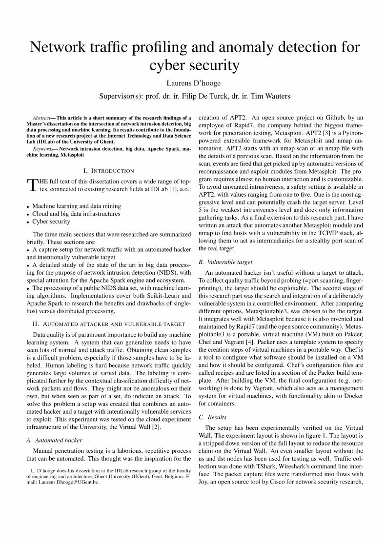
The core processing engine in this dissertation is ApacheSpark, the successor of Apache Hadoop. Spark is an in-memorybig data engine, with three layers (see figure 2). The Spark Core,which provides shared functionality for the four libraries on topof it. Those libraries are Spark-SQL for SQL-database-like pro-cessing of data, Spark Streaming for real-time event processing(micro-batch streaming), Spark-ML with distributed implemen-tations of machine learning algorithms and GraphX for graphprocessing. The third component is the scheduler to distributethe data and the work to the worker nodes. Spark is flexible andcan work with Apache YARN, Apache Mesos or its standalonescheduler.
Fig. 2. The Spark ecosystem
The main abstraction underlying Spark is the resilient, dis-tributed data set (RDD) on top of which more recent additionslike DataFrames and DataSets have been built. More efficientprocessing is continually introduced into the Spark project andits libraries. Two main projects stand out: the Spark-SQL cata-lyst optimizer works like a database query optimizer, receiving aprogrammed logical query plan, generating an optimized logicalquery plan and ultimately outputting Java bytecode that runs oneach machine. The other umbrella project concerned with opti-mization is called Project Tungsten. The research efforts underTungsten are focused on improving memory management andbinary processing (elimination of memory and garbage collec-tion overhead), cache-aware computation (making optimal useof on-die CPU cache) and code generation (improving serializa-tion and removing virtual function calls). These improvementsaim to make Spark the dominant big data processing engine fortimes to come.
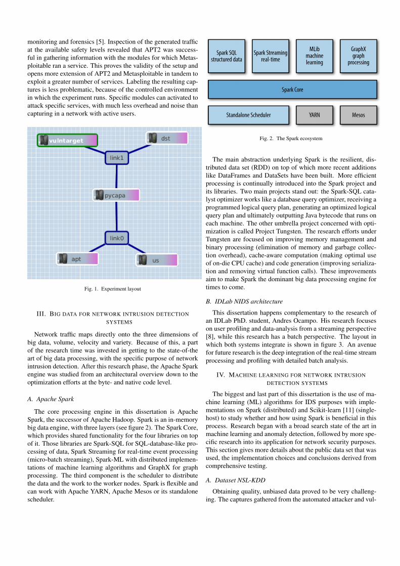
B. IDLab NIDS architecture
This dissertation happens complementary to the research ofan IDLab PhD. student, Andres Ocampo. His research focuseson user profiling and data-analysis from a streaming perspective[8], while this research has a batch perspective. The layout inwhich both systems integrate is shown in figure 3. An avenuefor future research is the deep integration of the real-time streamprocessing and profiling with detailed batch analysis.
IV. MACHINE LEARNING FOR NETWORK INTRUSIONDETECTION SYSTEMS
The biggest and last part of this dissertation is the use of ma-chine learning (ML) algorithms for IDS purposes with imple-mentations on Spark (distributed) and Scikit-learn [11] (single-host) to study whether and how using Spark is beneficial in thisprocess. Research began with a broad search state of the art inmachine learning and anomaly detection, followed by more spe-cific research into its application for network security purposes.This section gives more details about the public data set that wasused, the implementation choices and conclusions derived fromcomprehensive testing.
A. Dataset NSL-KDD
Obtaining quality, unbiased data proved to be very challeng-ing. The captures gathered from the automated attacker and vul-
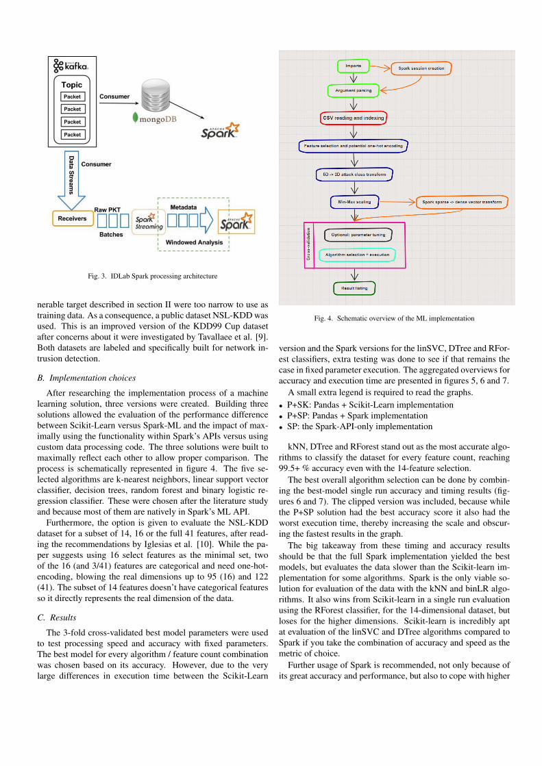
Fig. 3. IDLab Spark processing architecture
nerable target described in section II were too narrow to use astraining data. As a consequence, a public dataset NSL-KDD wasused. This is an improved version of the KDD99 Cup datasetafter concerns about it were investigated by Tavallaee et al. [9].Both datasets are labeled and specifically built for network in-trusion detection.
B. Implementation choices
After researching the implementation process of a machinelearning solution, three versions were created. Building threesolutions allowed the evaluation of the performance differencebetween Scikit-Learn versus Spark-ML and the impact of max-imally using the functionality within Spark’s APIs versus usingcustom data processing code. The three solutions were built tomaximally reflect each other to allow proper comparison. Theprocess is schematically represented in figure 4. The five se-lected algorithms are k-nearest neighbors, linear support vectorclassifier, decision trees, random forest and binary logistic re-gression classifier. These were chosen after the literature studyand because most of them are natively in Spark’s ML API.
Furthermore, the option is given to evaluate the NSL-KDDdataset for a subset of 14, 16 or the full 41 features, after read-ing the recommendations by Iglesias et al. [10]. While the pa-per suggests using 16 select features as the minimal set, twoof the 16 (and 3/41) features are categorical and need one-hot-encoding, blowing the real dimensions up to 95 (16) and 122(41). The subset of 14 features doesn’t have categorical featuresso it directly represents the real dimension of the data.
C. Results
The 3-fold cross-validated best model parameters were usedto test processing speed and accuracy with fixed parameters.The best model for every algorithm / feature count combinationwas chosen based on its accuracy. However, due to the verylarge differences in execution time between the Scikit-Learn
Fig. 4. Schematic overview of the ML implementation
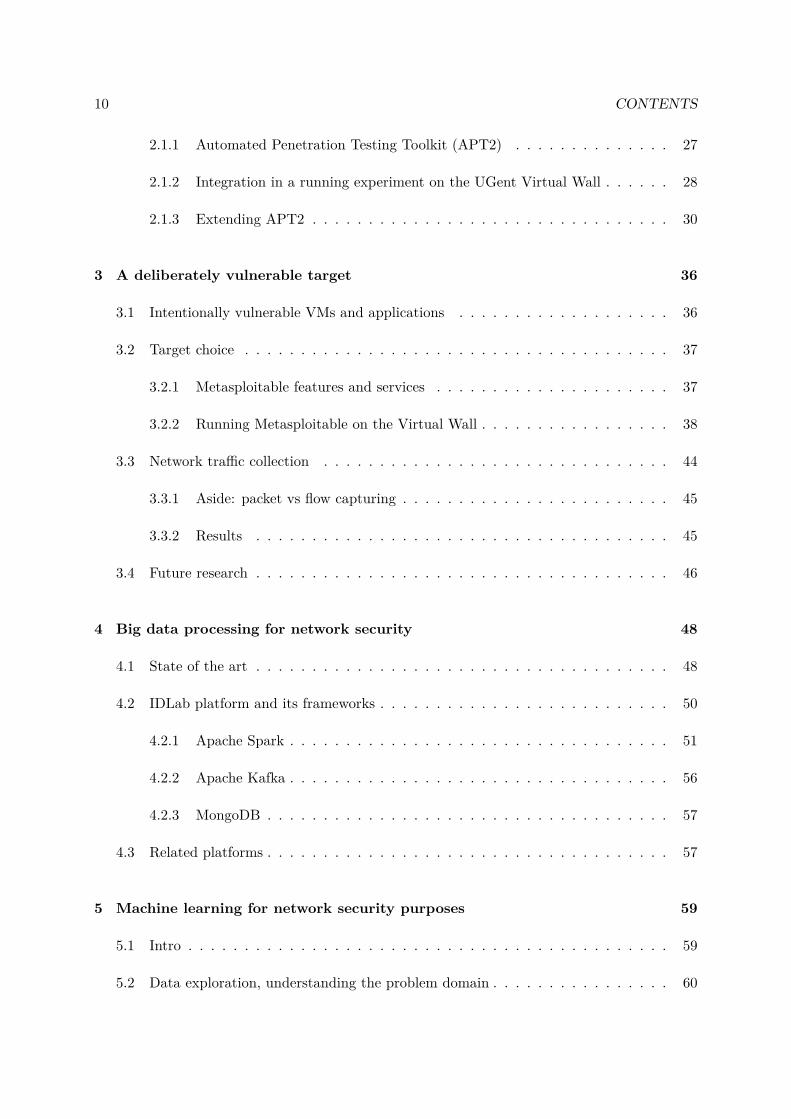
version and the Spark versions for the linSVC, DTree and RFor-est classifiers, extra testing was done to see if that remains thecase in fixed parameter execution. The aggregated overviews foraccuracy and execution time are presented in figures 5, 6 and 7.
A small extra legend is required to read the graphs.• P+SK: Pandas + Scikit-Learn implementation• P+SP: Pandas + Spark implementation• SP: the Spark-API-only implementation
kNN, DTree and RForest stand out as the most accurate algo-rithms to classify the dataset for every feature count, reaching99.5+ % accuracy even with the 14-feature selection.
The best overall algorithm selection can be done by combin-ing the best-model single run accuracy and timing results (fig-ures 6 and 7). The clipped version was included, because whilethe P+SP solution had the best accuracy score it also had theworst execution time, thereby increasing the scale and obscur-ing the fastest results in the graph.
The big takeaway from these timing and accuracy resultsshould be that the full Spark implementation yielded the bestmodels, but evaluates the data slower than the Scikit-learn im-plementation for some algorithms. Spark is the only viable so-lution for evaluation of the data with the kNN and binLR algo-rithms. It also wins from Scikit-learn in a single run evaluationusing the RForest classifier, for the 14-dimensional dataset, butloses for the higher dimensions. Scikit-learn is incredibly aptat evaluation of the linSVC and DTree algorithms compared toSpark if you take the combination of accuracy and speed as themetric of choice.
Further usage of Spark is recommended, not only because ofits great accuracy and performance, but also to cope with higher
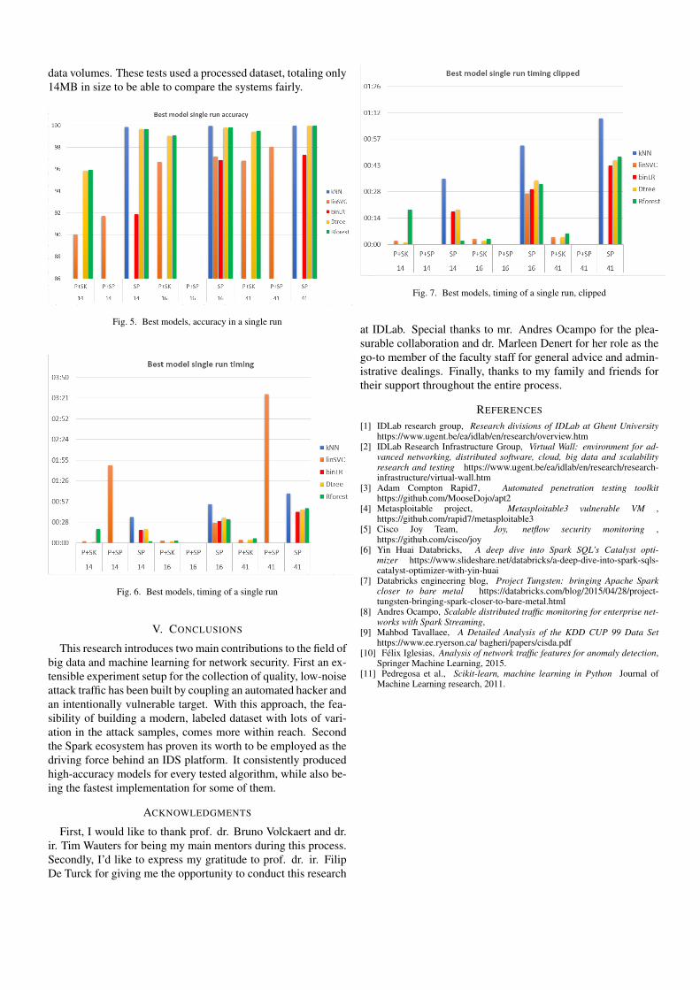
data volumes. These tests used a processed dataset, totaling only14MB in size to be able to compare the systems fairly.
Fig. 5. Best models, accuracy in a single run
Fig. 6. Best models, timing of a single run
V. CONCLUSIONS
This research introduces two main contributions to the field ofbig data and machine learning for network security. First an ex-tensible experiment setup for the collection of quality, low-noiseattack traffic has been built by coupling an automated hacker andan intentionally vulnerable target. With this approach, the fea-sibility of building a modern, labeled dataset with lots of vari-ation in the attack samples, comes more within reach. Secondthe Spark ecosystem has proven its worth to be employed as thedriving force behind an IDS platform. It consistently producedhigh-accuracy models for every tested algorithm, while also be-ing the fastest implementation for some of them.
ACKNOWLEDGMENTS
First, I would like to thank prof. dr. Bruno Volckaert and dr.ir. Tim Wauters for being my main mentors during this process.Secondly, I’d like to express my gratitude to prof. dr. ir. FilipDe Turck for giving me the opportunity to conduct this research
Fig. 7. Best models, timing of a single run, clipped
at IDLab. Special thanks to mr. Andres Ocampo for the plea-surable collaboration and dr. Marleen Denert for her role as thego-to member of the faculty staff for general advice and admin-istrative dealings. Finally, thanks to my family and friends fortheir support throughout the entire process.
REFERENCES
[1] IDLab research group, Research divisions of IDLab at Ghent Universityhttps://www.ugent.be/ea/idlab/en/research/overview.htm
[2] IDLab Research Infrastructure Group, Virtual Wall: environment for ad-vanced networking, distributed software, cloud, big data and scalabilityresearch and testing https://www.ugent.be/ea/idlab/en/research/research-infrastructure/virtual-wall.htm
[3] Adam Compton Rapid7, Automated penetration testing toolkithttps://github.com/MooseDojo/apt2
[4] Metasploitable project, Metasploitable3 vulnerable VM ,https://github.com/rapid7/metasploitable3
[5] Cisco Joy Team, Joy, netflow security monitoring ,https://github.com/cisco/joy
[6] Yin Huai Databricks, A deep dive into Spark SQL’s Catalyst opti-mizer https://www.slideshare.net/databricks/a-deep-dive-into-spark-sqls-catalyst-optimizer-with-yin-huai
[7] Databricks engineering blog, Project Tungsten: bringing Apache Sparkcloser to bare metal https://databricks.com/blog/2015/04/28/project-tungsten-bringing-spark-closer-to-bare-metal.html
[8] Andres Ocampo, Scalable distributed traffic monitoring for enterprise net-works with Spark Streaming,
[9] Mahbod Tavallaee, A Detailed Analysis of the KDD CUP 99 Data Sethttps://www.ee.ryerson.ca/ bagheri/papers/cisda.pdf
[10] Felix Iglesias, Analysis of network traffic features for anomaly detection,Springer Machine Learning, 2015.
[11] Pedregosa et al., Scikit-learn, machine learning in Python Journal ofMachine Learning research, 2011.

Contents
List of Figures 13
List of Tables 15
1 Introduction 17
1.1 Big data . . . . . . . . . . . . . . . . . . . . . . . . . . . . . . . . . . . . . . . . . 18
1.2 Paradigms of big data frameworks . . . . . . . . . . . . . . . . . . . . . . . . . . 19
1.2.1 Batch-only . . . . . . . . . . . . . . . . . . . . . . . . . . . . . . . . . . . 19
1.2.2 Stream-only . . . . . . . . . . . . . . . . . . . . . . . . . . . . . . . . . . . 19
1.2.3 Hybrid . . . . . . . . . . . . . . . . . . . . . . . . . . . . . . . . . . . . . . 21
1.3 Categories of cyber attacks . . . . . . . . . . . . . . . . . . . . . . . . . . . . . . 22
1.3.1 Denial of service . . . . . . . . . . . . . . . . . . . . . . . . . . . . . . . . 22
1.3.2 U2R . . . . . . . . . . . . . . . . . . . . . . . . . . . . . . . . . . . . . . . 23
1.3.3 R2L . . . . . . . . . . . . . . . . . . . . . . . . . . . . . . . . . . . . . . . 23
1.3.4 Probing . . . . . . . . . . . . . . . . . . . . . . . . . . . . . . . . . . . . . 23
1.4 Problem statement and purpose of this dissertation . . . . . . . . . . . . . . . . . 24
2 Building an automated attacker 26
2.1 Metasploit framework . . . . . . . . . . . . . . . . . . . . . . . . . . . . . . . . . 26
9
10 CONTENTS
2.1.1 Automated Penetration Testing Toolkit (APT2) . . . . . . . . . . . . . . 27
2.1.2 Integration in a running experiment on the UGent Virtual Wall . . . . . . 28
2.1.3 Extending APT2 . . . . . . . . . . . . . . . . . . . . . . . . . . . . . . . . 30
3 A deliberately vulnerable target 36
3.1 Intentionally vulnerable VMs and applications . . . . . . . . . . . . . . . . . . . 36
3.2 Target choice . . . . . . . . . . . . . . . . . . . . . . . . . . . . . . . . . . . . . . 37
3.2.1 Metasploitable features and services . . . . . . . . . . . . . . . . . . . . . 37
3.2.2 Running Metasploitable on the Virtual Wall . . . . . . . . . . . . . . . . . 38
3.3 Network traffic collection . . . . . . . . . . . . . . . . . . . . . . . . . . . . . . . 44
3.3.1 Aside: packet vs flow capturing . . . . . . . . . . . . . . . . . . . . . . . . 45
3.3.2 Results . . . . . . . . . . . . . . . . . . . . . . . . . . . . . . . . . . . . . 45
3.4 Future research . . . . . . . . . . . . . . . . . . . . . . . . . . . . . . . . . . . . . 46
4 Big data processing for network security 48
4.1 State of the art . . . . . . . . . . . . . . . . . . . . . . . . . . . . . . . . . . . . . 48
4.2 IDLab platform and its frameworks . . . . . . . . . . . . . . . . . . . . . . . . . . 50
4.2.1 Apache Spark . . . . . . . . . . . . . . . . . . . . . . . . . . . . . . . . . . 51
4.2.2 Apache Kafka . . . . . . . . . . . . . . . . . . . . . . . . . . . . . . . . . . 56
4.2.3 MongoDB . . . . . . . . . . . . . . . . . . . . . . . . . . . . . . . . . . . . 57
4.3 Related platforms . . . . . . . . . . . . . . . . . . . . . . . . . . . . . . . . . . . . 57
5 Machine learning for network security purposes 59
5.1 Intro . . . . . . . . . . . . . . . . . . . . . . . . . . . . . . . . . . . . . . . . . . . 59
5.2 Data exploration, understanding the problem domain . . . . . . . . . . . . . . . . 60
CONTENTS 11
5.2.1 Different levels of detail . . . . . . . . . . . . . . . . . . . . . . . . . . . . 60
5.2.2 Obtaining quality, unbiased data . . . . . . . . . . . . . . . . . . . . . . . 61
5.3 Steps in a machine learning solution . . . . . . . . . . . . . . . . . . . . . . . . . 61
5.3.1 First projects . . . . . . . . . . . . . . . . . . . . . . . . . . . . . . . . . . 61
5.3.2 Mathematical background, Coursera . . . . . . . . . . . . . . . . . . . . . 62
5.4 State of the art . . . . . . . . . . . . . . . . . . . . . . . . . . . . . . . . . . . . . 63
5.5 NSL-KDD . . . . . . . . . . . . . . . . . . . . . . . . . . . . . . . . . . . . . . . . 66
5.6 Implementation . . . . . . . . . . . . . . . . . . . . . . . . . . . . . . . . . . . . . 67
5.6.1 Pandas + Scikit-learn . . . . . . . . . . . . . . . . . . . . . . . . . . . . . 68
5.6.2 Spark . . . . . . . . . . . . . . . . . . . . . . . . . . . . . . . . . . . . . . 76
5.7 Benchmarking and results . . . . . . . . . . . . . . . . . . . . . . . . . . . . . . . 84
5.7.1 Methodology . . . . . . . . . . . . . . . . . . . . . . . . . . . . . . . . . . 84
5.7.2 Model parameter tuning results . . . . . . . . . . . . . . . . . . . . . . . . 85
5.7.3 Best models, single run results and ML conclusion . . . . . . . . . . . . . 87
5.7.4 Execution environment . . . . . . . . . . . . . . . . . . . . . . . . . . . . 90
6 Future work 91
6.1 Building a data set . . . . . . . . . . . . . . . . . . . . . . . . . . . . . . . . . . . 91
6.2 Working with different data sets . . . . . . . . . . . . . . . . . . . . . . . . . . . 92
6.3 More ML algorithms . . . . . . . . . . . . . . . . . . . . . . . . . . . . . . . . . . 92
6.4 User profile integration . . . . . . . . . . . . . . . . . . . . . . . . . . . . . . . . . 92
6.5 Big data performance and scaling . . . . . . . . . . . . . . . . . . . . . . . . . . . 92
6.6 Exploration of multi-model architectures . . . . . . . . . . . . . . . . . . . . . . . 93
7 Conclusion 94

12 CONTENTS
Bibliography 96
8 Appendix 101
8.1 A: ML parameter tuning results in tabular format . . . . . . . . . . . . . . . . . 101
8.2 B: ML optimal model testing . . . . . . . . . . . . . . . . . . . . . . . . . . . . . 103

List of Figures
1.1 Big data processing frameworks overseen by the Apache Software Foundation . . 18
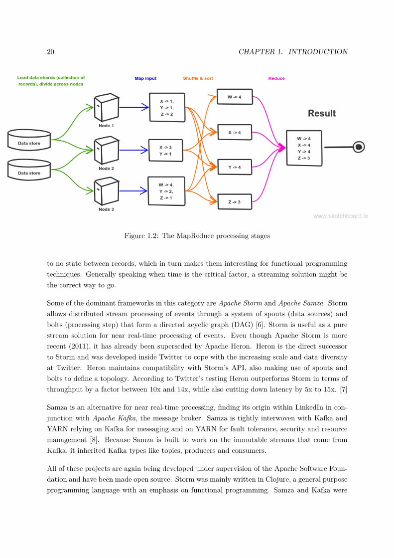
1.2 The MapReduce processing stages . . . . . . . . . . . . . . . . . . . . . . . . . . 20
2.1 Nodes in the full test layout . . . . . . . . . . . . . . . . . . . . . . . . . . . . . . 29
2.2 Nodes in the reduced layout . . . . . . . . . . . . . . . . . . . . . . . . . . . . . . 30
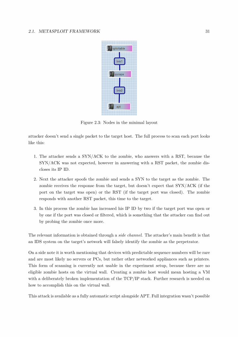
2.3 Nodes in the minimal layout . . . . . . . . . . . . . . . . . . . . . . . . . . . . . . 31
2.4 IP identification scanning . . . . . . . . . . . . . . . . . . . . . . . . . . . . . . . 32
4.1 The architecture used within IDlab . . . . . . . . . . . . . . . . . . . . . . . . . . 51
4.2 The architecture of the Spark framework, [1] . . . . . . . . . . . . . . . . . . . . 52
4.3 Spark’s execution model, [1] . . . . . . . . . . . . . . . . . . . . . . . . . . . . . . 53
4.4 Catalyst optimizer, [2] . . . . . . . . . . . . . . . . . . . . . . . . . . . . . . . . . 54
4.5 Catalyst optimizer, [3] . . . . . . . . . . . . . . . . . . . . . . . . . . . . . . . . . 55
5.1 Diagram of the implementations . . . . . . . . . . . . . . . . . . . . . . . . . . . 68
5.2 Average best model accuracies . . . . . . . . . . . . . . . . . . . . . . . . . . . . . 86
5.3 Parameter tuning search times . . . . . . . . . . . . . . . . . . . . . . . . . . . . 87
5.4 Parameter tuning search times clipped at 1h30m . . . . . . . . . . . . . . . . . . 88
5.5 Best models, accuracy in a single run . . . . . . . . . . . . . . . . . . . . . . . . . 88
13

14 LIST OF FIGURES
5.6 Best models, timing of a single run . . . . . . . . . . . . . . . . . . . . . . . . . . 89
5.7 Best models, timing of a single run, clipped . . . . . . . . . . . . . . . . . . . . . 90
List of Tables
3.1 summary of intentionally vulnerable practice targets . . . . . . . . . . . . . . . . 37
3.2 summary of the attack traffic captures . . . . . . . . . . . . . . . . . . . . . . . . 45
3.3 summary of the normal traffic captures . . . . . . . . . . . . . . . . . . . . . . . . 46
5.1 ML algorithms parameter tuning ranges . . . . . . . . . . . . . . . . . . . . . . . 85
8.1 kNN parameter tuning best models and search time . . . . . . . . . . . . . . . . 101
8.2 linSVC parameter tuning best models and search time . . . . . . . . . . . . . . . 102
8.3 binLR parameter tuning best models and search time . . . . . . . . . . . . . . . 102
8.4 DTree parameter tuning best models and search time . . . . . . . . . . . . . . . . 102
8.5 RForest parameter tuning best models and search time . . . . . . . . . . . . . . . 103
8.6 kNN best models accuracy and runtime . . . . . . . . . . . . . . . . . . . . . . . 103
8.7 linSVC best models accuracy and runtime . . . . . . . . . . . . . . . . . . . . . 103
8.8 binLR best models accuracy and runtime . . . . . . . . . . . . . . . . . . . . . . 104
8.9 DTree best models accuracy and runtime . . . . . . . . . . . . . . . . . . . . . . 104
8.10 RForest best models accuracy and runtime . . . . . . . . . . . . . . . . . . . . . 104
15
List of Listings
1 Metasploit Python MSFRPC interaction . . . . . . . . . . . . . . . . . . . . . . . 342 Python nmap automation . . . . . . . . . . . . . . . . . . . . . . . . . . . . . . . 353 Packer build template: builders section . . . . . . . . . . . . . . . . . . . . . . . . 404 Packer build template: provisioners section . . . . . . . . . . . . . . . . . . . . . 415 Packer build template: post-processors . . . . . . . . . . . . . . . . . . . . . . . . 416 Packer build template: user-defined variables . . . . . . . . . . . . . . . . . . . . 427 Chef: Metasploit iptables recipe . . . . . . . . . . . . . . . . . . . . . . . . . . . . 438 Vagrantfile with additional configuration (a.o. VM networking) . . . . . . . . . . 449 Pandas + Scikit-learn solution: imports . . . . . . . . . . . . . . . . . . . . . . . 6910 Pandas + Scikit-learn solution: argument parsing . . . . . . . . . . . . . . . . . . 7011 Pandas + Scikit-learn solution: reading CSV and indexing . . . . . . . . . . . . . 7112 Pandas + Scikit-learn solution: feature selection . . . . . . . . . . . . . . . . . . 7213 Pandas + Scikit-learn solution: binarize attack classes . . . . . . . . . . . . . . . 7314 Pandas + Scikit-learn solution: min-max scaling . . . . . . . . . . . . . . . . . . 7315 Pandas + Scikit-learn solution: cross-validation . . . . . . . . . . . . . . . . . . . 7416 Pandas + Scikit-learn solution: kNN parameter tuning . . . . . . . . . . . . . . . 7517 Pandas + Scikit-learn solution: kNN fixed parameter . . . . . . . . . . . . . . . . 7518 Pandas + Scikit-learn solution: result processing . . . . . . . . . . . . . . . . . . 7619 Full Spark solution: imports . . . . . . . . . . . . . . . . . . . . . . . . . . . . . . 7720 Full Spark solution: Spark session building . . . . . . . . . . . . . . . . . . . . . 7821 Full Spark solution: typed CSV reading . . . . . . . . . . . . . . . . . . . . . . . 7822 Full Spark solution: indexing and binarizing attack classes . . . . . . . . . . . . . 8023 Full Spark solution: feature selection . . . . . . . . . . . . . . . . . . . . . . . . . 8124 Full Spark solution: min-max scaling . . . . . . . . . . . . . . . . . . . . . . . . . 8125 Full Spark solution: sparse to dense vector udf . . . . . . . . . . . . . . . . . . . 8226 Full Spark solution: routing logic . . . . . . . . . . . . . . . . . . . . . . . . . . . 8327 Full Spark solution: kNN with cross-validation and parameter tuning . . . . . . . 8328 Full Spark solution: kNN with fixed parameters . . . . . . . . . . . . . . . . . . . 84
16
1Introduction
Nowadays no year goes by without some major security breaches. Equifax, Sony, Netflix, Yahooand the Democratic National Committee are just the (prominent) tip of the iceberg, hacked inthe last five years [4]. One important thing nearly all hacks have in common is the remote aspect.They can be carried out from anywhere on the planet with internet access. This means thatat some point the traffic carrying the attack was in transit on the internet. More importantlyit wasn’t caught along the way! The content of this master dissertation is at the intersectionof cyber security, big data processing and machine learning. This text describes the processand results of the two major research parts. The first part is the creation of a setup for thegeneration of high-quality traffic samples with baseline and attack traffic. The second part isthe comparison between using Apache Spark, a distributed big data processing engine and asingle-host processing system to run machine learning algorithms for classifying network trafficinto normal and attack traffic.
This dissertation starts with the introduction of several concepts in the big data and networksecurity domains, followed by a problem statement. The next two chapters give a detaileddescription of an experiment setup, which includes an automated attacker (based on the Metas-ploit Framework) and a deliberately vulnerable target. The second chapter ends with the resultsof letting the automated hacker attack the vulnerable target in terms of network traffic. Thesecond part of this dissertation spans another two chapters. The first one is a deep dive intobig data for network security and the Spark processing engine. The second chapter details the
17
18 CHAPTER 1. INTRODUCTION
Figure 1.1: Big data processing frameworks overseen by the Apache Software Foundation
process and results of developing machine learning solutions both in- and outside the Sparkecosystem. The final chapter before the conclusion is an introduction to the research areas thathave opened themselves as a result of this work.
1.1 Big data
What is big data? At what point is data considered big? How does the processing of big datadiffer from the traditional methods? These are only some of the relevant questions regardingbig data. The three main traits to determine whether you’re working with big data are volume,variety and velocity. When the combination of these dimensions exceeds a threshold, the storageand processing of the data becomes problematic. At that point we start to use the term bigdata. It is not possible to delineate the precise points along the three dimensions, where big datastarts to come into play. From a business perspective one could argue that big data techniquesare considered when it is no longer financially interesting to use a single high-powered machine.The wording of that sentence also reveals the main difference between ”normal” and big datamethods. Big data solutions spread the workload over a collection of machines. Key aspects ofthe big data solutions are distributed storage systems and distributed processing models.
1.2. PARADIGMS OF BIG DATA FRAMEWORKS 19
1.2 Paradigms of big data frameworks
Current solutions are on either side of the dichotomy between batch-only and stream-only frame-works, with some hybrid forms emerging as well.
1.2.1 Batch-only
The batch processing approach is the most well-known strategy. The key characteristic of thismodel is that it operates on a large, static data set that was persisted (stored) earlier. The datais often a historic collection of records, collected over a certain time period, e.g. one month ofproduct orders. The most prevalent framework in this category was Apache Hadoop. Forgedin 2006 from the Google file system and the MapReduce processing model, it gained tractionthrough its wins in big data sorting competitions. Today the Hadoop framework consists offour components [5]: Hadoop Common libraries and utilities, Hadoop Distributed File System(HDFS), Hadoop YARN (Yet Another Resource Negotiator) and an implementation of theMapReduce processing model. The MapReduce API consists of only two functions map() andreduce(). The total processing model is split into four stages (see figure 1.2). The processingpart of the Hadoop framework has been replaced by Apache Spark. More information on ApacheSpark can be found in the hybrids paragraph and in chapter 4.
1. Read input files and split them into records for the available processing nodes
2. Call the map function to extract a key-value pair from each record
3. Shuffle and sort all the pairs by their key
4. Call the reduce function to iterate over the sorted set of key-value pairs and output theresult
The Hadoop framework is primarily written in the Java language. Its development is opensource and is overseen by the Apache Software Foundation.
1.2.2 Stream-only
The stream-only strategy is found opposite to the batch processing strategy. The key charac-teristics are operation on an unbounded amount of data as it enters the system, processing onlyone item at a time. A slight variation of this model is micro-batching and while it by definitioncan’t be called true stream processing, it comes close. These systems end up holding very little
20 CHAPTER 1. INTRODUCTION
Figure 1.2: The MapReduce processing stages
to no state between records, which in turn makes them interesting for functional programmingtechniques. Generally speaking when time is the critical factor, a streaming solution might bethe correct way to go.
Some of the dominant frameworks in this category are Apache Storm and Apache Samza. Stormallows distributed stream processing of events through a system of spouts (data sources) andbolts (processing step) that form a directed acyclic graph (DAG) [6]. Storm is useful as a purestream solution for near real-time processing of events. Even though Apache Storm is morerecent (2011), it has already been superseded by Apache Heron. Heron is the direct successorto Storm and was developed inside Twitter to cope with the increasing scale and data diversityat Twitter. Heron maintains compatibility with Storm’s API, also making use of spouts andbolts to define a topology. According to Twitter’s testing Heron outperforms Storm in terms ofthroughput by a factor between 10x and 14x, while also cutting down latency by 5x to 15x. [7]
Samza is an alternative for near real-time processing, finding its origin within LinkedIn in con-junction with Apache Kafka, the message broker. Samza is tightly interwoven with Kafka andYARN relying on Kafka for messaging and on YARN for fault tolerance, security and resourcemanagement [8]. Because Samza is built to work on the immutable streams that come fromKafka, it inherited Kafka types like topics, producers and consumers.
All of these projects are again being developed under supervision of the Apache Software Foun-dation and have been made open source. Storm was mainly written in Clojure, a general purposeprogramming language with an emphasis on functional programming. Samza and Kafka were
1.2. PARADIGMS OF BIG DATA FRAMEWORKS 21
written in the Java and Scala languages.
1.2.3 Hybrid
As a natural consequence of the dichotomy between the former two approaches, a third optionhas emerged in an effort to combine the virtues of the distinct models. Hybrid frameworks offerthe ability to work with both batches and streams, while providing APIs that can work with thedifferent types. The goal is to simplify the way of interacting with the fundamentally differentdata types. Two currently popular solutions include Apache Spark, which has been used for thisresearch, and Apache Flink. Spark started as a batch-oriented framework and added streaming,while Flink started as a streaming framework and added batches. Apache Spark can be seenas the second generation of the Hadoop framework, more specifically as a replacement for themap-reduce implementation of Hadoop. The project first saw light in 2009 at the University ofBerkeley, California and was open sourced in 2010. By 2009 Hadoop was already proving itsworth [9], but despite the strides it made in big data processing, it wasn’t flawless. The maingripe users of Hadoop had, was the disk I/O (input/output) required by Hadoop. A map-reducejob starts with reading files before the map operation and outputs to files after the reduceoperation. Storage speeds were the main limiting factor in processing. That’s where Sparkcomes in with its in-memory processing that removes writing of intermittent results to disk.Spark also comes with other optimizations, but the in-memory processing is the main benefit.The inner workings of Spark will be discussed in more detail in a later chapter, because thisdetection system is built on Spark. As the successor to the hugely popular Hadoop framework,Spark is touted as the framework-to-adopt for big data processing. Spark became a top-levelApache project in February of 2014. Its Apache mirror is available on Github and the frameworkis mostly written in Scala and Java.
Flink is a stream-oriented framework that can also work with batches. The core concept in Flinkis its predication on the Kappa architecture. In the Kappa architecture everything is a stream. Areal stream has no presumed end, whereas a batch is seen as a finite stream. This is in contrast tothe older Lambda architecture where batches played the central role. Flink works with streamsas immutable series without bounds upon which operations can be performed that generate otherstreams [10]. Streams enter the system from sources and leave through sinks. Spark, based onLambda architecture treats batches as the primary type and streams are micro-batches. For realstream processing this can be undesirable and that’s where Flink fits in, flipping the hierarchyand treating real streams as its foundation. Flink started as a fork of a research project at threeuniversities in or close to Berlin. It was adopted by the Apache Software Foundation in theincubator stage in 2014. The main languages used to develop Flink are Scala and Java. Aninteresting comparison between the performance of Spark, Flink and Storm has been done ina research paper by a group of Yahoo employees. A real world pipeline was built with Apache
22 CHAPTER 1. INTRODUCTION
Kafka, the Redis data and the three aforementioned processing frameworks to store, relay andtransform events in Javascript Object Notaton (JSON) format. After testing they conclude thatFlink and Storm behave like real streaming engines, offering near real-time processing of events.Spark streaming is disadvantaged in terms of latency because of its micro-batching design, butthat is what makes enables it to handle higher event throughput [11].
1.3 Categories of cyber attacks
The DARPA (Defense Advanced Research Projects Agency) 1998 data set for intrusion detectionevaluation contains captures of real attacks against a network and its hosts. The sample containsthe four main attack types, which are Denial of Service (Dos), User to Root (U2R), Remote toLocal (R2L) and Probe. The DARPA 1999 data set added an additional category, exfiltrationattempts of sensitive data.
1.3.1 Denial of service
DoS is an attack type where the goal is to prevent access to a service. Networked applicationscan be targeted in a variety of ways, the two most common are: crashing the service by sendingit malformed requests that trigger runtime exceptions which in turn aren’t handled properly oroverloading the service with requests. An attack against the application is also called a layer 7attack, because the application layer is the seventh in the OSI network stack. Network basedattacks are most common in the form of using all available bandwidth of the target by sending somany requests that the network can’t relay the requests in time. Those attacks are volume basedand there are no structural solutions other than to increase the network capacity. Because of therequired amount of ingress bandwidth to bring a service down, a collection of hosts is often usedto attack a single target. This variation is called a distributed denial of service attack (DDoS).Modern DDoS attacks either leverage a huge amount of hosts (e.g. the Mirai IoT botnet [12]) ormake use of amplification to increase the attack bandwidth. Forms of amplification are, amongothers, DNS amplification [13] (for instance through AXFR queries on open resolvers) and NTPamplification [14]. The effectiveness of the amplification is measured by the amplifying factor,e.g. a 100 byte request that results in a 5000 byte response has an amplifying factor of 50.
Lastly there are attacks using the characteristics of network protocols and software implemen-tations that build on that protocol. A well-known example is the slow loris attack against webservers, nested in a broader category of HTTP-flooding attacks [15]. A partial HTTP headeris sent to establish a connection to the server, after which the minimum amount of data tokeep the connection alive is sent, simulating an excruciatingly slow client. Once all availableconnections on the web server are exhausted, no other clients can connect. Because I couldn’t
1.3. CATEGORIES OF CYBER ATTACKS 23
find a recent paper describing the impact of this attack, I ran it myself. The most prominenttarget, susceptible to this attack is Apache HTTP server, which at the time of writing still hasa 42,41% market share (450.000.000 million servers) [16]. Even the latest version (albeit withdefault configuration) becomes unreachable against an attacker opening 1000 connections everyfive seconds. This attack uses little bandwidth and is easily carried out by a single attacker.
1.3.2 U2R
User to root attacks attempt to gain full control over the target, rather than making it unavail-able. Every interaction point with clients is a potential entry point. These attacks are sent overthe network, but its their payload that makes them dangerous, not the traffic that carries it.The payload includes an exploit against a vulnerability in the service. Buffer overruns are atypical vulnerability that can lead to total takeover. From a network perspective these attacksare not as obvious as denial of service. A full attack can consist of only a handful of packets,while the impact is much more severe. The low packet footprint is due to the availability of thebinaries of the programs, including web servers or other public facing services. It has also beenshown that an exploit can be built and run, even without access to the binary [17].
1.3.3 R2L
Remote to local attacks try to insert the attacker as a host in a network. Once the attackerhas access to the network he can try to increase his foothold, by spreading laterally and /or vertically (provided he obtains administrator credentials or abuses a privilege escalationvulnerability). Common ways to enter a subnetwork are insufficiently secured services (suchas FTP or password guessing. The noise caused by these attacks varies with the strategy, e.g.brute force password guessing generates more network requests than an FTP exploit.
1.3.4 Probing
Located early in the attack cycle, the probing phase uses tools to map the attack surface of thetarget. Nmap is an example of a probing tool. It’s a network scanner with a host of options tocustomize the results. Included features are host discovery, port scanning, version and operatingsystem (OS) detection. Nessus and OpenVas are, in contrast to nmap, not just network scanners.They are vulnerability scanners, which means that in addition to the network portion they alsotry to identify if a service is running a vulnerable software version. In the first stages of thisthesis I have focused on probing, because this attack stage is a prerequisite to the others (exceptDoS).

24 CHAPTER 1. INTRODUCTION
1.4 Problem statement and purpose of this dissertation
There are a lot of commercial e.g. FireEye or AlienVault and non-commercial e.g. snort orfail2ban (network) intrusion detection and prevention systems (IDS / IPS) available. Theyoperate mainly as signature based systems or statistical anomaly based systems. Detectionsystems only signal (possible) intrusion attempts, while their preventing counterparts activelytry to block the attempt.
Solutions that work with signatures have the advantage of high detection rates, but only forpreviously encountered attacks. These systems won’t be able to detect zero day attacks if thatattack has a sufficiently different fingerprint compared to the known set of fingerprints. Thissignature approach needs a signature database that is constantly updated with new attacks orvariants of old attacks [18]. The failure to protect against novelty and inertia associated withupdating the knowledge base, weaken this system against a motivated attacker.
Statistical solutions operate on meta data of the network traffic to find outliers. This approachis able to detect novel attacks, but it has issues generalizing. The rule set has to be changingconstantly to remain effective. Intrusion detection systems that cause too many false positiveswill eventually be ignored by network administrators. A third option is profile-based IDS, wherea baseline is established, based on historic data.
An additional distinction has to be made based on the location of the system that evaluates thenetwork traffic. Common options include a central network intrusion detection system (NIDS)that looks at the traffic of the entire (sub)network or a host-based solution that runs on everyindividual machine. IDS can be viewed as a component of the larger security information andevent management (SIEM) architecture. SIEMs are broader in the sense that they includeall kinds of logging output and their main focus is monitoring operation, of which securitymonitoring is one part.
This thesis will focus on the generalization of detection systems and the advantages of modernbig data frameworks as the foundation on which new tools are built. Ultimately the goal istwofold, designing a system that can detect anomalous behavior without signatures and provingthat big data platforms are capable as the processing platform for this task in modern, large-scale networks. This system is also suitable for novel data-intensive application use cases such ashealthcare, smart cities, internet of things (IoT) networks, manufacturing or smart grids. Thenecessary adaptation would be gaining insight in the data of those problem domains. This thesisis part of the setup of a new research project at Ghent University, aimed at building a platformfor anomaly detection. My work is the batch processing arm of said platform, complementaryto mr. Ocampo’s stream processing.
The stages of this dissertation include:

1.4. PROBLEM STATEMENT AND PURPOSE OF THIS DISSERTATION 25
1. Research into the state of the art of intrusion detection systems w.r.t. big data and machinelearning
2. Building an automated attacker and integrating it into the current experiment layout (see 2.1)
3. Building a vulnerable target and integrating that as well
4. Investigation into the design and added value of using the Spark big data framework forprocessing
5. Application of the chosen machine learning techniques to build a predictive model
6. Future work, including integration with the profile-based approach that is under develop-ment within the research group
2Building an automated attacker
This chapter is a report of the build process for an automated attacker and its integration in anexisting experiment. Most of the content is centered around the automation of the Metasploitframework, the comprehensive, open-source tool for exploitation. This automation is facilitatedthrough the Metasploit Remote Procedure Calling (MSFRPC) API.
2.1 Metasploit framework
The Metasploit framework is the world’s most used penetration testing framework. Its inceptiondates back to 2003 when it was created by its founder H.D. Moore. In 2009 the Metasploitproject was acquired by Rapid7, a private company offering a range of cyber security products.Development of the Metasploit platform is open source, available on Github under the BSD-3-clause license. The original was written in Perl, but a rewrite in Ruby happened early on andRuby is still the language to develop for the platform today.On Linux-based systems, especially headless ones (without peripherals, accessible only throughSSH or a similar protocol), the preferred way of interacting with the Metasploit framework isthrough the msfconsole or msfcli programs. Msfconsole offers an interactive session to run apenetration test all the way from host discovery to getting a root shell on the target machine.The exploitation phase of the penetration testing process with Metasploit can be summarized
26

2.1. METASPLOIT FRAMEWORK 27
as follows
1. Use tools for host discovery like nmap or Metasploit’s discovery modules.
2. Use the results of the host discovery to run vulnerability scanning tools like Nessus, Open-Vas or Nexpose against (part of) the found hosts to assemble a list of potential targetservices.
3. Choose a suitable exploit for a vulnerable service found in step 2. The exploits are writtenby a community of pentesters, sometimes the same people who submitted a CommonVulnerability and Exposure (CVE) entry to prove the validity of their finding.
4. Pick a payload to run on the compromised host. The most feature rich payload is themeterpreter shell to run arbitrary commands on the target. It injects itself as a dynami-cally loaded library (dll) into an existing process and leaves no traces on disk. Moreovermeterpreter sets up a Transport Layer Security v1 (TLSv1) session to communicate andload custom plugins [19].
5. Using an encoder to mask the attack traffic in an attempt to fool IDS systems.
6. Running the combination of exploit, payload and encoder to attack the target.
Metasploit became the most popular because of its modular architecture, allowing the combina-tion of any exploit with any payload and any encoding. Currently 3664 exploits are registeredin Rapid7’s exploit-db [20]. These are all integrated in the pro version of the Metasploit frame-work.The penetration testing process is laborious and often repetitive. This is in part due to therequired interaction between the attacker and his tools. A service might be exploitable, but notwith default settings. The knowledge of the attacker is still a very important factor so he needsthe possibility to interact with his tools. Certain tasks however can be automated, especiallywith regards to information gathering. Automating this attacker was a first step in this thesis.
2.1.1 Automated Penetration Testing Toolkit (APT2)
Adam Compton, a Rapid7 employee laid the foundation for an automation framework for Metas-ploit. The tool integrates nmap and Metasploit through the Metasploit RPC interface, to auto-mate the chain of host and service discovery, choosing suitable exploits, exploiting the target(s)and post-exploitation steps. I have forked the project to my own Github to make modificationsand additions. This work started with learning the architecture of APT2 and its capabilities.The project is written in Python, which added some additional complexity, because I had little
28 CHAPTER 2. BUILDING AN AUTOMATED ATTACKER
to no Python experience previous to this.APT2 has several features that contribute to the automation
• The ability to import results from nmap, Nexpose or Nessus as a starting point
• An option to run an nmap scan with chosen options to generate a starting point
• A knowledge base with the parsed results from the starting point
• An event-based system that looks through the knowledge base and triggers upon findingprotocols, ports or self-defined features of interest.
• A collection of modules, each of which reacts to a certain collection of events to load itselfas a viable candidate for automatic execution
• Automatic execution of the modules that were loaded and interaction with the outputgenerated by the Metasploit framework to add to the knowledge base and build a report
• The liberty to write a configuration file and feeding that to APT2 to avoid any userinteraction
The exploratory tests with APT2 and Metasploit were performed on my home network insidean Ubuntu 16.04 Virtual Machine (VM). I chose this setup because it bears similarity with theoperating system that would be available as a VM on the universities’ infrastructure.
After understanding the inner workings of APT2, some time was required to get it to work onmy system, mostly pertaining to running the tool as a non-privileged user. Upon achieving astable environment that hosted all the dependencies of APT2, Metasploit and nmap, I bundledthe setup in a Markdown manual and a shell script file. Those resources were subsequentlyused to build the same environment on the stock Ubuntu 16.04 LTS image that is available onthe UGent Virtual Wall, a testbed for researchers. More information about that environmentcan be found in the subsection about the integration. The main practical difficulties with thepreparation of an attacking VM were finding a suitable Metasploit version that was capable ofrunning headless and finding and installing the required dependencies for APT2.
2.1.2 Integration in a running experiment on the UGent Virtual Wall
My research is happening complementary to the work of PhD student Andres Ocampo. Histopic is big data processing for network traffic with a focus on streaming and user profiling. Mywork is focused on batch processing and simulation. When I started there were some captures ofsimulated normal traffic like web browsing, email and FTP traffic, but there was no attack traffic
2.1. METASPLOIT FRAMEWORK 29
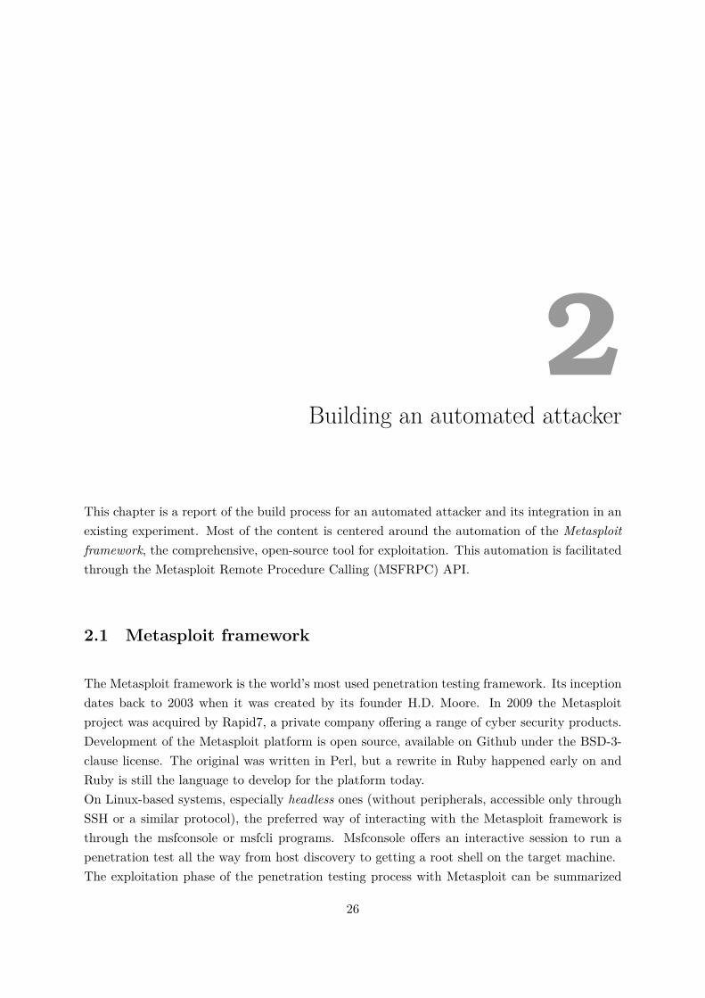
Figure 2.1: Nodes in the full test layout
yet. We had a need for clean attack traffic, meaning that it should be possible to distinguishbetween attack and non-attack traffic. The VMs of the experiment on the virtual wall are silentif my attacker is not running, so they won’t pollute an attack data capture.
The full layout can be seen in the figure 2.1.
A brief description of the components
• link0-2: represent the subnetworks 192.168.x.y, with configuration of the connected nodes
• pycapa: a central network capture node, in charge of relaying between the three /24subnets
• us: the user node, simulates multiple physical hosts and is used to replay previous capturesto the destination
• apt: my custom VM, running the aforementioned setup. The traffic of attack sessions canbe captured for replay from the us node
• dst: the target host to attack
• mongodb: the long-term storage database for traffic captures
30 CHAPTER 2. BUILDING AN AUTOMATED ATTACKER
Figure 2.2: Nodes in the reduced layout
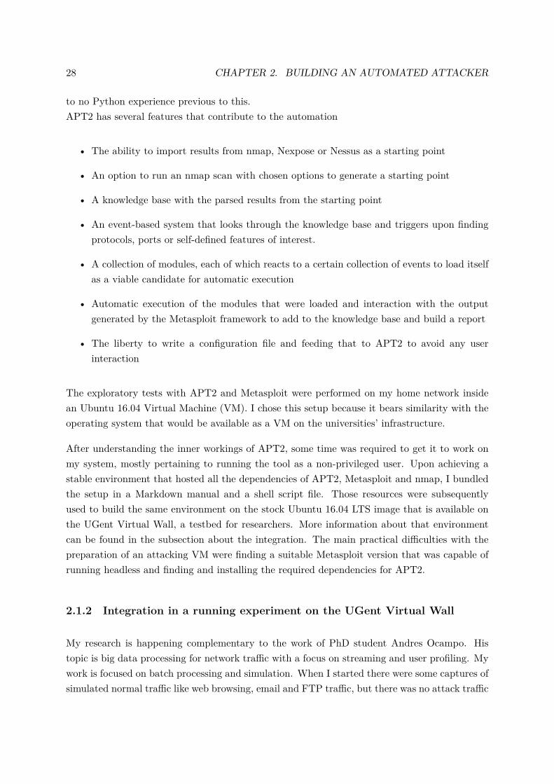
• spark: the node running the Spark big data framework
• kafka: the node running the Kafka message broker
The destination node has some deficiencies. It doesn’t permanently host other services besidesssh. This meant that probing the dst node yields no interesting results. There are no vulnerableservices to attack. What is available is only some basic information gathering. To overcomethis problem, I have finished the integration of the Metasploitable project, an intentionallyvulnerable VM as a target into the experiment layout (details in chapter 3). Until there wassuch a vulnerable node, successful U2R or exfiltration attacks couldn’t be captured.
The nodes that make up the big data processing layout aren’t necessary yet. To avoid unnec-essarily claiming resources from the Virtual Wall, I’m working in a stripped layout that lookslike 2.2 or in the even smaller 2.3 . For more information regarding the architecture of the dataprocessing, I’d like to refer to the big data chapter.
2.1.3 Extending APT2
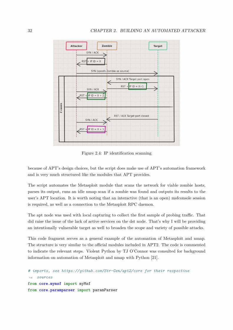
APT2 can start off with an nmap scan, but only certain types of scanning are available dueto the way the nmap statement gets built. A more challenging case was made by one of mymentors, when he brought up the concept of TCP idle scanning. TCP idle scanning is a stealthyapproach to scan a target, but there is a prerequisite. This prerequisite is the existence of azombie host in the network. That zombie host must be in an idle network state for this approachto work and more importantly needs to have predictable IP sequence numbers (IP ID). The real
2.1. METASPLOIT FRAMEWORK 31
Figure 2.3: Nodes in the minimal layout
attacker doesn’t send a single packet to the target host. The full process to scan each port lookslike this:
1. The attacker sends a SYN/ACK to the zombie, who answers with a RST, because theSYN/ACK was not expected, however in answering with a RST packet, the zombie dis-closes its IP ID.
2. Next the attacker spoofs the zombie and sends a SYN to the target as the zombie. Thezombie receives the response from the target, but doesn’t expect that SYN/ACK (if theport on the target was open) or the RST (if the target port was closed). The zombieresponds with another RST packet, this time to the target.
3. In this process the zombie has increased his IP ID by two if the target port was open orby one if the port was closed or filtered, which is something that the attacker can find outby probing the zombie once more.
The relevant information is obtained through a side channel. The attacker’s main benefit is thatan IDS system on the target’s network will falsely identify the zombie as the perpetrator.
On a side note it is worth mentioning that devices with predictable sequence numbers will be rareand are most likely no servers or PCs, but rather other networked appliances such as printers.This form of scanning is currently not usable in the experiment setup, because there are noeligible zombie hosts on the virtual wall. Creating a zombie host would mean hosting a VMwith a deliberately broken implementation of the TCP/IP stack. Further research is needed onhow to accomplish this on the virtual wall.
This attack is available as a fully automatic script alongside APT. Full integration wasn’t possible
32 CHAPTER 2. BUILDING AN AUTOMATED ATTACKER
Figure 2.4: IP identification scanning
because of APT’s design choices, but the script does make use of APT’s automation frameworkand is very much structured like the modules that APT provides.
The script automates the Metasploit module that scans the network for viable zombie hosts,parses its output, runs an idle nmap scan if a zombie was found and outputs its results to theuser’s APT location. It is worth noting that an interactive (that is an open) msfconsole sessionis required, as well as a connection to the Metasploit RPC daemon.
The apt node was used with local capturing to collect the first sample of probing traffic. Thatdid raise the issue of the lack of active services on the dst node. That’s why I will be providingan intentionally vulnerable target as well to broaden the scope and variety of possible attacks.
This code fragment serves as a general example of the automation of Metasploit and nmap.The structure is very similar to the official modules included in APT2. The code is commentedto indicate the relevant steps. Violent Python by TJ O’Connor was consulted for backgroundinformation on automation of Metasploit and nmap with Python [21].
# imports, see https://github.com/Str-Gen/apt2/core for their respectivesources↪→
from core.mymsf import myMsffrom core.paramparser import paramParser
2.1. METASPLOIT FRAMEWORK 33
from core.mynmap import mynmapfrom core.utils import Display
# parse parametersp = paramParser()p.parseParameters(sys.argv)
# printer setuppp = pprint.PrettyPrinter(indent=2)pp.pprint(p.config)
This is the normal way to interact with msfrpc. Connect to the service, check if the connectionwas successful, pick a module and fill its options for the right target, run it and collect the result.It is worth noting that in order to collect the result, the msfrpc service had to be started in aninteractive msfconsole session.
# connect to Metasploit RPC servicemsf = myMsf(host=p.config['msfhost'], port=p.config['msfport'],
user=p.config['msfuser'], password=p.config['msfpass'])↪→
if not msf.isAuthenticated():sys.exit("Authentication failure to msfprc, QUITTING\n")
# metasploit load module & provide argumentsmsf.execute("use auxiliary/scanner/ip/ipidseq\n")msf.execute("set RHOSTS %s\n" % p.config["rhosts"])msf.execute("set THREADS %d\n" % p.config["threads"])msf.execute("set RPORT %d\n" % p.config["rport"])print("Running metasploit module auxiliary/scanner/ip/ipidseq with:\n")print("RHOSTS => %s THREADS => %d RPORT => %d\n" %(p.config["rhosts"],
p.config["threads"], p.config["rport"]))↪→
# run metasploit modulemsf.execute("run\n")msf.sleep(5)result = msf.getResult()pp.pprint(result)msf.cleanup()
lines = result.splitlines()
34 CHAPTER 2. BUILDING AN AUTOMATED ATTACKER
pp.pprint(lines)
Listing 1: Metasploit Python MSFRPC interaction
Hosts on the network can be used as zombies if their IP identifiers are sequential. The outputof the Metasploit module is a text, showing a host on every line and a message to say if it is apotential zombie. A regular expression for an IPv4 address is used to extract the zombie’s IP.After that a location is created to store the result of the scan.
# extract potential zombie hostspattern = re.compile("(((25[0-
5]|2[0-4][0-9]|[01]?[0-9][0-9]?).){3}(25[0-5]|2[0-4][0-9]|[01]?[0-9][0-9]?))'sIPID sequence class: Incremental!")
↪→
↪→
ip_matches = []for l in lines:
match = pattern.search(l)if match is not None:
ip_match = match.group(1)print ip_match, "is a potential zombie"ip_matches.append(ip_match)
# Create an output folder for these results if it doesn't exist yettry:
os.makedirs(os.path.expanduser("~/.apt2/ipidseq/"))except OSError as e:
if e.errno != errno.EEXIST:raise
p.config["proofsDir"] = os.path.expanduser("~/.apt2/ipidseq/")
The final part is an example of nmap automation. The parsed results of running the Metasploitmodule are included to designate a zombie for the scan. The scan results are stored in thelocation that was set earlier. Every step of the process is automated. The attack can belaunched with a single shell command.
# create an nmap instancen = mynmap(p.config,Display())
scan_results = {}if ip_matches:
flagstring = "-sI %s %s" % (ip_matches[0],p.config["nmapargs"])print flagstring,"\n"
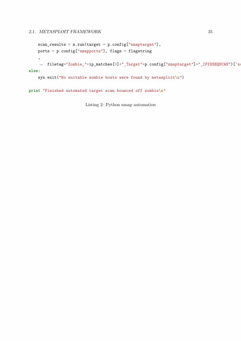
2.1. METASPLOIT FRAMEWORK 35
scan_results = n.run(target = p.config["nmaptarget"],ports = p.config["nmapports"], flags = flagstring,
filetag="Zombie_"+ip_matches[0]+"_Target"+p.config["nmaptarget"]+"_IPIDSEQSCAN")['scan']↪→
else:sys.exit("No suitable zombie hosts were found by metasploit\n")
print "Finished automated target scan bounced off zombie\n"
Listing 2: Python nmap automation
3A deliberately vulnerable target
A shortcoming in the existing experiment was discovered after running the fully automatedattacker, described in the previous chapter. The previous target, the dst machine, only runs theSSH daemon to provide login functionality. This lack of available services led to a tiny capturefile ( 250 KB) when probing the system. APT2 couldn’t fire events for interesting ports andservices, because all but one are closed. This severely restricts the scope of possible attacks.In order to solve this problem, a more interesting target was needed. More interesting means atarget that hosts intentionally vulnerable services, to gain maximum benefit from the automaticexploitation capabilities of APT2.
3.1 Intentionally vulnerable VMs and applications
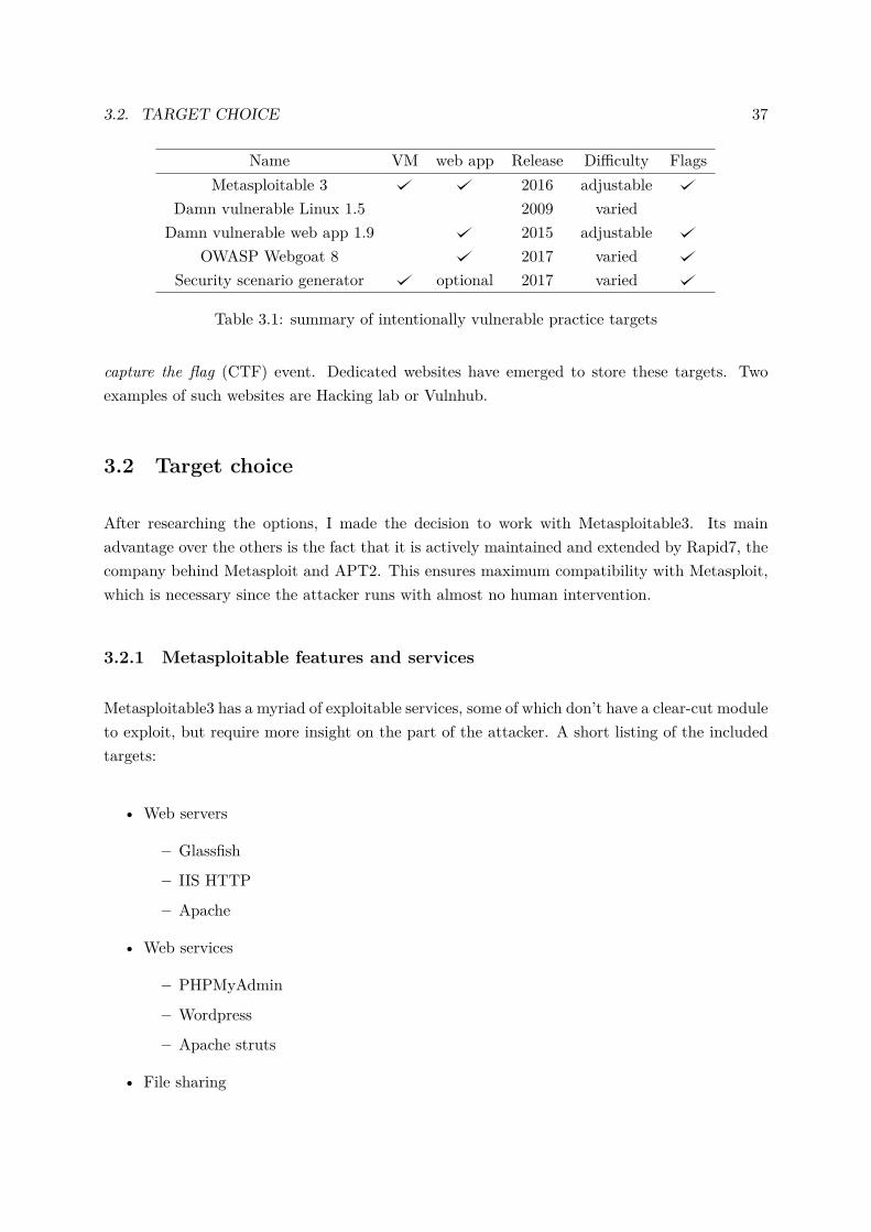
Students and professionals aspiring to become penetration tester have several options at theirdisposal to grow their skill. Over the years a collection of deliberately vulnerable virtual machinesand standalone applications have been developed to practice different security aspects. Table3.1 gives a brief listing of some available options.
This table only lists some of the popular or interesting options, but it is worth noting that thereis a very large collection of machines like these. These are often created for a single security
36
3.2. TARGET CHOICE 37
Name VM web app Release Difficulty FlagsMetasploitable 3 2016 adjustable
Damn vulnerable Linux 1.5 2009 variedDamn vulnerable web app 1.9 2015 adjustable
OWASP Webgoat 8 2017 variedSecurity scenario generator optional 2017 varied
Table 3.1: summary of intentionally vulnerable practice targets
capture the flag (CTF) event. Dedicated websites have emerged to store these targets. Twoexamples of such websites are Hacking lab or Vulnhub.
3.2 Target choice
After researching the options, I made the decision to work with Metasploitable3. Its mainadvantage over the others is the fact that it is actively maintained and extended by Rapid7, thecompany behind Metasploit and APT2. This ensures maximum compatibility with Metasploit,which is necessary since the attacker runs with almost no human intervention.
3.2.1 Metasploitable features and services
Metasploitable3 has a myriad of exploitable services, some of which don’t have a clear-cut moduleto exploit, but require more insight on the part of the attacker. A short listing of the includedtargets:
• Web servers
– Glassfish
– IIS HTTP
– Apache
• Web services
– PHPMyAdmin
– Wordpress
– Apache struts
• File sharing

38 CHAPTER 3. A DELIBERATELY VULNERABLE TARGET
– SMB
– IIS FTP
• Databases
– MySQL
– ElasticSearch
• SSH, SNMP daemon and more
Metasploitable is an impressive testing environment that is under active development, whichmade it a well-suited choice.
3.2.2 Running Metasploitable on the Virtual Wall
After recognizing the benefits of Metasploitable, a working version for the virtual wall had tobe built. The project’s wiki on Github gives a short overview of the required soft- and hardwareto build Metasploitable for your platform.
The two software requirements to build the virtual machine Packer and Vagrant. Packer is atool that provides hardware abstraction for the creator of the VM through the ability to usethe same configuration file on different machines. Vagrant is a tool to create portable, virtualenvironments by gluing together other tools like Puppet or Chef for provisioning and Virtualbox,Docker or Hyper-V as providers.
The Metasploitable virtual machine can be built to run for the Virtualbox and VMWare plat-forms.
Hardware requirements for the Windows Metasploitable include CPU virtualization support(Intel VT-X or AMD-V), 4.5 GB of RAM and 65 GB available disk space. The Ubuntu Linuxflavor of Metasploitable requires the same CPU support as well as 4 GB of RAM and 40 GB offree disk space [22]. The disk space requirement is a recommendation that can be reduced inthe build template.
Those requirements are steep, but necessary to run the feature-rich target. Some issues havearisen in trying to run this on the Virtual Wall. The most glaring issue is the virtualization insidean already virtualized environment. In contrast to the automated attacker it is not possible tomodify the stock Ubuntu image that is available for everyone on the wall. Doing that wouldessentially amount to rebuilding Metasploitable from scratch.
The preparation of the stock Ubuntu VM with the required software is available in the appendix.
3.2. TARGET CHOICE 39
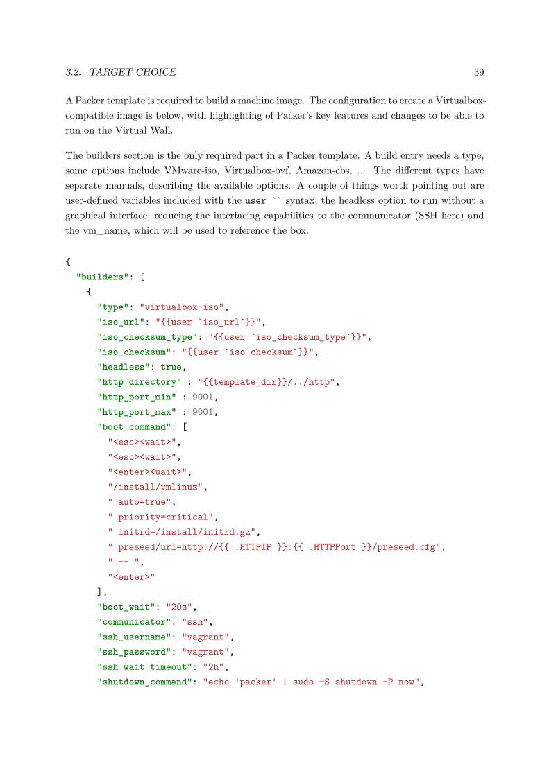
A Packer template is required to build a machine image. The configuration to create a Virtualbox-compatible image is below, with highlighting of Packer’s key features and changes to be able torun on the Virtual Wall.
The builders section is the only required part in a Packer template. A build entry needs a type,some options include VMware-iso, Virtualbox-ovf, Amazon-ebs, ... The different types haveseparate manuals, describing the available options. A couple of things worth pointing out areuser-defined variables included with the user `` syntax, the headless option to run without agraphical interface, reducing the interfacing capabilities to the communicator (SSH here) andthe vm_name, which will be used to reference the box.
{"builders": [{
"type": "virtualbox-iso","iso_url": "{{user `iso_url`}}","iso_checksum_type": "{{user `iso_checksum_type`}}","iso_checksum": "{{user `iso_checksum`}}","headless": true,"http_directory" : "{{template_dir}}/../http","http_port_min" : 9001,"http_port_max" : 9001,"boot_command": ["<esc><wait>","<esc><wait>","<enter><wait>","/install/vmlinuz"," auto=true"," priority=critical"," initrd=/install/initrd.gz"," preseed/url=http://{{ .HTTPIP }}:{{ .HTTPPort }}/preseed.cfg"," -- ","<enter>"
],"boot_wait": "20s","communicator": "ssh","ssh_username": "vagrant","ssh_password": "vagrant","ssh_wait_timeout": "2h","shutdown_command": "echo 'packer' | sudo -S shutdown -P now",
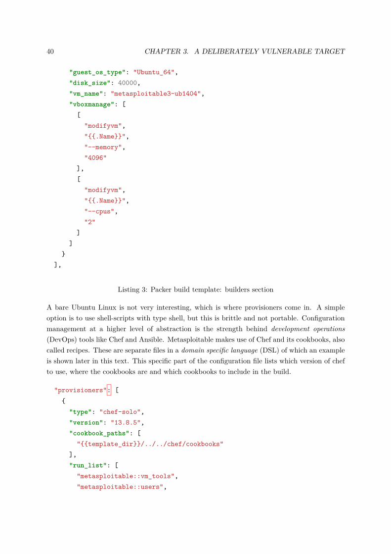
40 CHAPTER 3. A DELIBERATELY VULNERABLE TARGET
"guest_os_type": "Ubuntu_64","disk_size": 40000,"vm_name": "metasploitable3-ub1404","vboxmanage": [[
"modifyvm","{{.Name}}","--memory","4096"
],[
"modifyvm","{{.Name}}","--cpus","2"
]]
}],
Listing 3: Packer build template: builders section
A bare Ubuntu Linux is not very interesting, which is where provisioners come in. A simpleoption is to use shell-scripts with type shell, but this is brittle and not portable. Configurationmanagement at a higher level of abstraction is the strength behind development operations(DevOps) tools like Chef and Ansible. Metasploitable makes use of Chef and its cookbooks, alsocalled recipes. These are separate files in a domain specific language (DSL) of which an exampleis shown later in this text. This specific part of the configuration file lists which version of chefto use, where the cookbooks are and which cookbooks to include in the build.
"provisioners": [{
"type": "chef-solo","version": "13.8.5","cookbook_paths": ["{{template_dir}}/../../chef/cookbooks"
],"run_list": ["metasploitable::vm_tools","metasploitable::users",
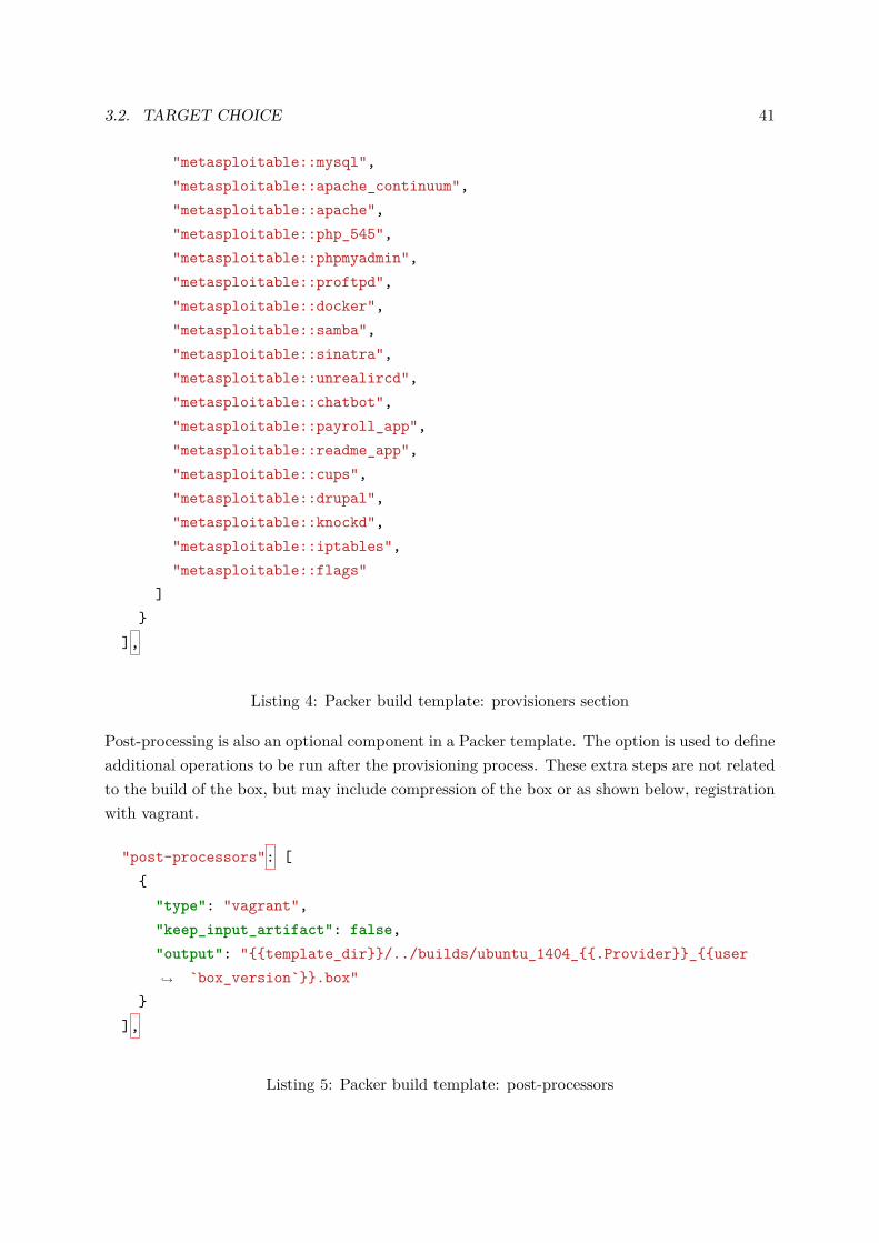
3.2. TARGET CHOICE 41
"metasploitable::mysql","metasploitable::apache_continuum","metasploitable::apache","metasploitable::php_545","metasploitable::phpmyadmin","metasploitable::proftpd","metasploitable::docker","metasploitable::samba","metasploitable::sinatra","metasploitable::unrealircd","metasploitable::chatbot","metasploitable::payroll_app","metasploitable::readme_app","metasploitable::cups","metasploitable::drupal","metasploitable::knockd","metasploitable::iptables","metasploitable::flags"
]}
],
Listing 4: Packer build template: provisioners section
Post-processing is also an optional component in a Packer template. The option is used to defineadditional operations to be run after the provisioning process. These extra steps are not relatedto the build of the box, but may include compression of the box or as shown below, registrationwith vagrant.
"post-processors": [{
"type": "vagrant","keep_input_artifact": false,"output": "{{template_dir}}/../builds/ubuntu_1404_{{.Provider}}_{{user
`box_version`}}.box"↪→
}],
Listing 5: Packer build template: post-processors
42 CHAPTER 3. A DELIBERATELY VULNERABLE TARGET
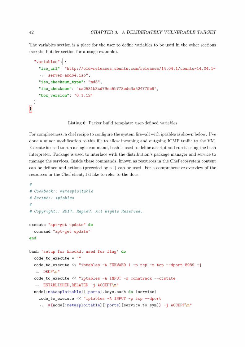
The variables section is a place for the user to define variables to be used in the other sections(see the builder section for a usage example).
"variables": {"iso_url": "http://old-releases.ubuntu.com/releases/14.04.1/ubuntu-14.04.1-
server-amd64.iso",↪→
"iso_checksum_type": "md5","iso_checksum": "ca2531b8cd79ea5b778ede3a524779b9","box_version": "0.1.12"
}}
Listing 6: Packer build template: user-defined variables
For completeness, a chef recipe to configure the system firewall with iptables is shown below. I’vedone a minor modification to this file to allow incoming and outgoing ICMP traffic to the VM.Execute is used to run a single command, bash is used to define a script and run it using the bashinterpreter. Package is used to interface with the distribution’s package manager and service tomanage the services. Inside these commands, known as resources in the Chef ecosystem contentcan be defined and actions (preceded by a :) can be used. For a comprehensive overview of theresources in the Chef client, I’d like to refer to the docs.
## Cookbook:: metasploitable# Recipe:: iptables## Copyright:: 2017, Rapid7, All Rights Reserved.
execute "apt-get update" docommand "apt-get update"
end
bash 'setup for knockd, used for flag' docode_to_execute = ""code_to_execute << "iptables -A FORWARD 1 -p tcp -m tcp --dport 8989 -j
DROP\n"↪→
code_to_execute << "iptables -A INPUT -m conntrack --ctstateESTABLISHED,RELATED -j ACCEPT\n"↪→
node[:metasploitable][:ports].keys.each do |service|code_to_execute << "iptables -A INPUT -p tcp --dport
#{node[:metasploitable][:ports][service.to_sym]} -j ACCEPT\n"↪→
3.2. TARGET CHOICE 43
endcode_to_execute << "iptables -A INPUT -p tcp --dport 22 -j ACCEPT\n"code_to_execute << "iptables -A INPUT -p icmp -j ACCEPT\n"code_to_execute << "iptables -A OUTPUT -p icmp -j ACCEPT\n"code_to_execute << "iptables -A INPUT -j DROP\n"code code_to_execute
end
package 'iptables-persistent' doaction :install
end
service 'iptables-persistent' doaction [:enable, :start]
end
Listing 7: Chef: Metasploit iptables recipe
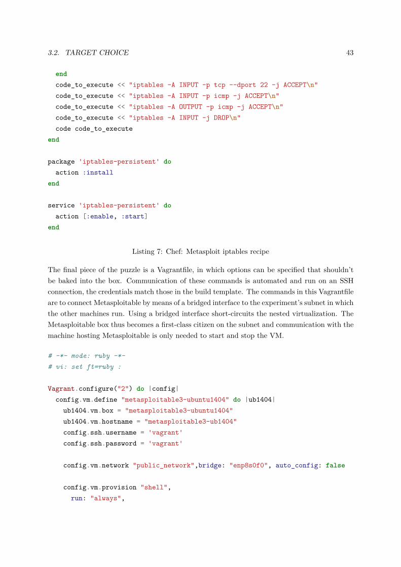
The final piece of the puzzle is a Vagrantfile, in which options can be specified that shouldn’tbe baked into the box. Communication of these commands is automated and run on an SSHconnection, the credentials match those in the build template. The commands in this Vagrantfileare to connect Metasploitable by means of a bridged interface to the experiment’s subnet in whichthe other machines run. Using a bridged interface short-circuits the nested virtualization. TheMetasploitable box thus becomes a first-class citizen on the subnet and communication with themachine hosting Metasploitable is only needed to start and stop the VM.
# -*- mode: ruby -*-# vi: set ft=ruby :
Vagrant.configure("2") do |config|config.vm.define "metasploitable3-ubuntu1404" do |ub1404|ub1404.vm.box = "metasploitable3-ubuntu1404"ub1404.vm.hostname = "metasploitable3-ub1404"config.ssh.username = 'vagrant'config.ssh.password = 'vagrant'
config.vm.network "public_network",bridge: "enp8s0f0", auto_config: false
config.vm.provision "shell",run: "always",
44 CHAPTER 3. A DELIBERATELY VULNERABLE TARGET
inline: "ifconfig eth1 192.168.1.4 netmask 255.255.255.0 up"
config.vm.provision "shell",run: "always",inline: "route add default gw 192.168.1.1 eth1"
config.vm.provision "shell",run: "always",inline: "ip route add 192.168.0.0/16 via 192.168.1.1 dev eth1"
ub1404.vm.provider "virtualbox" do |v|v.name = "Metasploitable3-ubuntu1404"v.memory = 4096
endend
end
Listing 8: Vagrantfile with additional configuration (a.o. VM networking)
To recapitulate this section: Metasploitable 3 is built with portability and maintainability inmind. The vulnerable VM uses Packer templates to support multiple VM executors and callsChef to automate the machine configuration. At the highest level Vagrant is used to managethe created boxes and automate environment specific setup. This hierarchy of tools allows torun Metasploitable with a single command vagrant up after building the box.
3.3 Network traffic collection
After completing the vulnerable VM, I tested it by running the automated attacker against it.The attacker has various levels of intrusiveness, ranging from level 5 (safest) to level 1 (use allmodules).
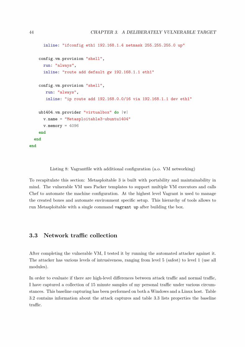
In order to evaluate if there are high-level differences between attack traffic and normal traffic,I have captured a collection of 15 minute samples of my personal traffic under various circum-stances. This baseline capturing has been performed on both a Windows and a Linux host. Table3.2 contains information about the attack captures and table 3.3 lists properties the baselinetraffic.
3.3. NETWORK TRAFFIC COLLECTION 45
Intrusiveness Scan type .pcap size .joy sizelevel 5 TCP SYN 612.6 KB 1.2 MBlevel 5 TCP Connect 539.1 KB 966.8 KBlevel 4 TCP SYN 631.2 KB 1.2 MBlevel 4 TCP Connect 564.5 KB 982.6 KBlevel 3 TCP SYN 632.3 KB 1.2 MBlevel 3 TCP Connect 570.3 KB 984.7 KBlevel 2 TCP SYN 637.6 KB 1.2 MBlevel 2 TCP Connect 574.4 KB 986.0 KBlevel 1 TCP SYN 632.9 KB 1.2 MBlevel 1 TCP Connect 568.4 KB 987.7 KB
Table 3.2: summary of the attack traffic captures
3.3.1 Aside: packet vs flow capturing
Wireshark captures raw packets and stores them in packet capture files (.pcap or .pcapng). Rawpackets contain a lot of information, but nothing aggregated. Aggregated info is useful thoughe.g. to get connection duration, total connection size. That is why the second paradigm ofnetwork traffic capturing is flow-based capturing. Internet Protocol Flow information Export(IPFIX) is the standardized IETF protocol for export of IP flow information. This standardis open, but was derived from what Cisco Systems already had as a proprietary feature for itshardware. Writing a new system to restitch the packets back into flows would be redundant,for such software already exists. I have used an open source project by Cisco called Joy. Joyfocuses on capturing and analyzing flow data, with the purpose of network research, forensicsand security monitoring [23]. It can ingest .pcap files and its output is in Javascript ObjectNotation (JSON) format.
3.3.2 Results
Two things stand out in these basic statistics, the first of which is the inverse relation betweenpacket capture and flow capture in terms of size. Because each attack starts with a port scanof the target, every probe initiates a connection, because it targets a different port. The TCPConnect scan type uses the connect() system call and finishes the TCP handshake. If a con-nection is established, it gets broken off by the scanning host. TCP SYN scanning doesn’t evenestablish a full connection. The scan uses raw packets and notices if a port is open, filtered orclosed based on the first packet response of the server (in order SYN/ACK, RST, no answereven after retransmit or ICMP unreachable). A SYN/ACK response is immediately followed bya RST [24].
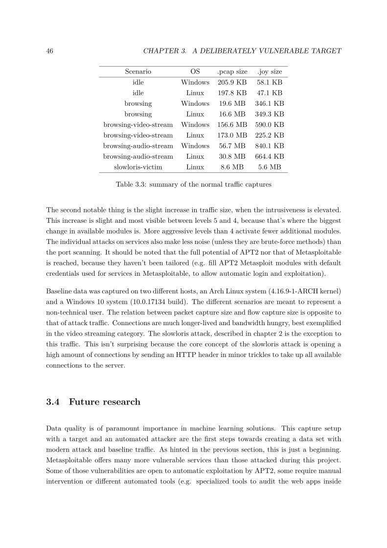
46 CHAPTER 3. A DELIBERATELY VULNERABLE TARGET
Scenario OS .pcap size .joy sizeidle Windows 205.9 KB 58.1 KBidle Linux 197.8 KB 47.1 KB
browsing Windows 19.6 MB 346.1 KBbrowsing Linux 16.6 MB 349.3 KB
browsing-video-stream Windows 156.6 MB 590.0 KBbrowsing-video-stream Linux 173.0 MB 225.2 KBbrowsing-audio-stream Windows 56.7 MB 840.1 KBbrowsing-audio-stream Linux 30.8 MB 664.4 KB
slowloris-victim Linux 8.6 MB 5.6 MB
Table 3.3: summary of the normal traffic captures
The second notable thing is the slight increase in traffic size, when the intrusiveness is elevated.This increase is slight and most visible between levels 5 and 4, because that’s where the biggestchange in available modules is. More aggressive levels than 4 activate fewer additional modules.The individual attacks on services also make less noise (unless they are brute-force methods) thanthe port scanning. It should be noted that the full potential of APT2 nor that of Metasploitableis reached, because they haven’t been tailored (e.g. fill APT2 Metasploit modules with defaultcredentials used for services in Metasploitable, to allow automatic login and exploitation).
Baseline data was captured on two different hosts, an Arch Linux system (4.16.9-1-ARCH kernel)and a Windows 10 system (10.0.17134 build). The different scenarios are meant to represent anon-technical user. The relation between packet capture size and flow capture size is opposite tothat of attack traffic. Connections are much longer-lived and bandwidth hungry, best exemplifiedin the video streaming category. The slowloris attack, described in chapter 2 is the exception tothis traffic. This isn’t surprising because the core concept of the slowloris attack is opening ahigh amount of connections by sending an HTTP header in minor trickles to take up all availableconnections to the server.
3.4 Future research
Data quality is of paramount importance in machine learning solutions. This capture setupwith a target and an automated attacker are the first steps towards creating a data set withmodern attack and baseline traffic. As hinted in the previous section, this is just a beginning.Metasploitable offers many more vulnerable services than those attacked during this project.Some of those vulnerabilities are open to automatic exploitation by APT2, some require manualintervention or different automated tools (e.g. specialized tools to audit the web apps inside

3.4. FUTURE RESEARCH 47
Metasploitable). Other attacks won’t be automatable, because they require careful crafting ortoo many interactions between the attacker and his tools. Nevertheless it is a valid goal tointroduce reliable, portable automation. Metasploitable can be extended with other vulnera-ble services, because of its flexible architecture. APT2 can be adapted in tandem with moreMetasploit modules.
Getting real attack traffic isn’t sufficient though and feature engineering, both on the packetand flow level are equally important.
4Big data processing for network security
Network traffic collection quickly becomes a big data story. By recalling the three main char-acteristics of big data: volume, velocity and variety and overlaying these on modern computernetworks, it becomes clear that a singular machine won’t be able to store, let alone process thisamount of data. Consider the following example: a small subnetwork of 10 physical nodes, eachwith their own 1 Gbit/s network interface card (NIC). Even if the averaged load across a 24hour period on the NICs is only 0.1 percent of their capacity, that is still 1 Mbit/s. Over theperiod of one day that amounts to 108 GB of network traffic for only those 10 hosts. A quicknapkin math calculation like this, highlights the volume aspect of network traffic. Networkinghardware becomes cheaper and capable of processing a higher bit rates to cater to the increasingneeds of the consumers, indicating the increase in velocity. Network traffic is varied by its natureencapsulating a vast collection of protocols and their characteristics. This chapter includes anoverview of the state of the art in big data application for network traffic, an in-depth look atthe IDlab platform, its frameworks and some comparable projects.
4.1 State of the art
During my research I’ve assembled and read a collection of academic papers about specific topicson the intersection of traffic analysis and big data. These papers approach the current situation
48
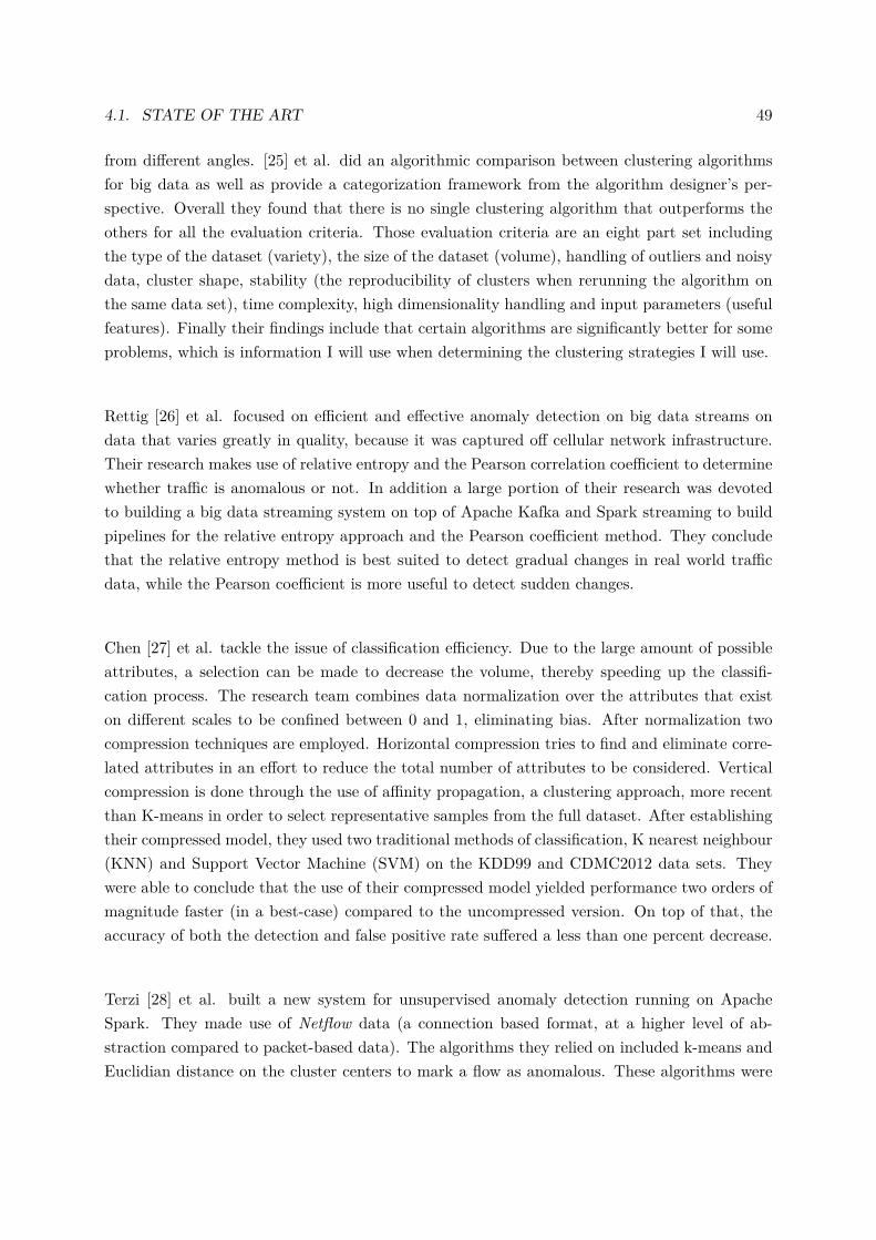
4.1. STATE OF THE ART 49
from different angles. [25] et al. did an algorithmic comparison between clustering algorithmsfor big data as well as provide a categorization framework from the algorithm designer’s per-spective. Overall they found that there is no single clustering algorithm that outperforms theothers for all the evaluation criteria. Those evaluation criteria are an eight part set includingthe type of the dataset (variety), the size of the dataset (volume), handling of outliers and noisydata, cluster shape, stability (the reproducibility of clusters when rerunning the algorithm onthe same data set), time complexity, high dimensionality handling and input parameters (usefulfeatures). Finally their findings include that certain algorithms are significantly better for someproblems, which is information I will use when determining the clustering strategies I will use.
Rettig [26] et al. focused on efficient and effective anomaly detection on big data streams ondata that varies greatly in quality, because it was captured off cellular network infrastructure.Their research makes use of relative entropy and the Pearson correlation coefficient to determinewhether traffic is anomalous or not. In addition a large portion of their research was devotedto building a big data streaming system on top of Apache Kafka and Spark streaming to buildpipelines for the relative entropy approach and the Pearson coefficient method. They concludethat the relative entropy method is best suited to detect gradual changes in real world trafficdata, while the Pearson coefficient is more useful to detect sudden changes.
Chen [27] et al. tackle the issue of classification efficiency. Due to the large amount of possibleattributes, a selection can be made to decrease the volume, thereby speeding up the classifi-cation process. The research team combines data normalization over the attributes that existon different scales to be confined between 0 and 1, eliminating bias. After normalization twocompression techniques are employed. Horizontal compression tries to find and eliminate corre-lated attributes in an effort to reduce the total number of attributes to be considered. Verticalcompression is done through the use of affinity propagation, a clustering approach, more recentthan K-means in order to select representative samples from the full dataset. After establishingtheir compressed model, they used two traditional methods of classification, K nearest neighbour(KNN) and Support Vector Machine (SVM) on the KDD99 and CDMC2012 data sets. Theywere able to conclude that the use of their compressed model yielded performance two orders ofmagnitude faster (in a best-case) compared to the uncompressed version. On top of that, theaccuracy of both the detection and false positive rate suffered a less than one percent decrease.
Terzi [28] et al. built a new system for unsupervised anomaly detection running on ApacheSpark. They made use of Netflow data (a connection based format, at a higher level of ab-straction compared to packet-based data). The algorithms they relied on included k-means andEuclidian distance on the cluster centers to mark a flow as anomalous. These algorithms were
50 CHAPTER 4. BIG DATA PROCESSING FOR NETWORK SECURITY
preceded by a temporal splitting, aggregation by source IP and normalization of the netflowdata. They conclude that their system reached 96% accuracy.
Rana [29] et al. have collected methods for outlier detection, with an emphasis on real-timeprocessing, but not only confined to the domain of traffic analysis. As stated in their paper’sconclusion, the main goal was to categorize and recommend available techniques such as statisti-cal, classification and clustering, to other researchers who have trouble deciding which techniqueto use.
Finally, Casas [30] et al. decided to devote their research project to the development of a bigdata analytics framework that is capable of both batch and stream processing. The streamingportion is underpinned by the Spark streaming framework and the batch portion is built onSpark and uses Cassandra as its data store. They tested their framework on the MAWILabdataset, a collection of 15 minute traces, collected on a daily basis on a backbone connectionbetween the United States and Japan. The research team used five available algorithms fromSpark’s machine learning library to train on the traffic. Further effort included benchmarkingtheir system, Big-DAMA, to a plain Spark cluster also with 12 nodes and a previous solutionby the same team using DBStream. They conclude that their system is able to store largeamounts of structured and unstructured data and is capable of processing that data, an orderof magnitude faster than a regular Spark cluster and significantly faster than their previoussolution.
This overview wraps up my state of the art analysis in big data, with special attention for itsuse in anomaly detection for network traffic.
4.2 IDLab platform and its frameworks
Ocampo [31] et al. presented an architecture for network traffic analysis, founded on Spark andSpark Streaming, backed by MongoDB and bound together by Apache Kafka. The architectureis capable of both batch- and stream processing.
The research also includes profiling users’ behavior, which I will delve deeper into in the finalchapter. In this chapter the focus is on the big data platform for which the main componentswill be examined in more detail.
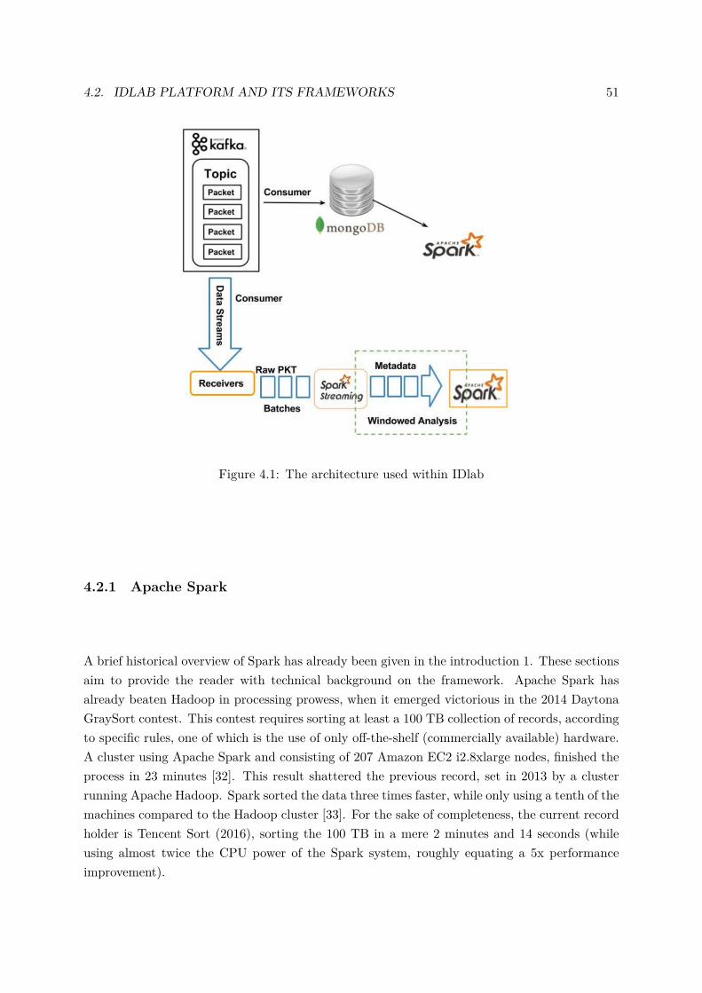
4.2. IDLAB PLATFORM AND ITS FRAMEWORKS 51
Figure 4.1: The architecture used within IDlab
4.2.1 Apache Spark
A brief historical overview of Spark has already been given in the introduction 1. These sectionsaim to provide the reader with technical background on the framework. Apache Spark hasalready beaten Hadoop in processing prowess, when it emerged victorious in the 2014 DaytonaGraySort contest. This contest requires sorting at least a 100 TB collection of records, accordingto specific rules, one of which is the use of only off-the-shelf (commercially available) hardware.A cluster using Apache Spark and consisting of 207 Amazon EC2 i2.8xlarge nodes, finished theprocess in 23 minutes [32]. This result shattered the previous record, set in 2013 by a clusterrunning Apache Hadoop. Spark sorted the data three times faster, while only using a tenth of themachines compared to the Hadoop cluster [33]. For the sake of completeness, the current recordholder is Tencent Sort (2016), sorting the 100 TB in a mere 2 minutes and 14 seconds (whileusing almost twice the CPU power of the Spark system, roughly equating a 5x performanceimprovement).
52 CHAPTER 4. BIG DATA PROCESSING FOR NETWORK SECURITY
Figure 4.2: The architecture of the Spark framework, [1]
Components
Figure 4.2 shows the parts of the Spark system, the most important of which is the Spark core.The central concept in the Spark architecture are the resilient, distributed datasets (RDD). Asmentioned in 1 Spark improved over Hadoop with its in-memory capabilities. Spark’s API isavailable for the Java, Scala and Python languages. In this thesis the Python language willbe used to interface with Spark. This research is focused on batch processing and thereforemakes most use of the Spark SQL and Spark Mlib libraries. This research happens alongsideir. Ocampo’s work which focuses on stream analysis and profile derivation. The integrationstrategy for these two research avenues is documented in the final chapter 6.
RDD
The resilient component of RDD means that even if data in memory is lost, it can be recon-structed. The distributed aspect means that data is either stored in memory or on disk, spreadacross the cluster of machines. The dataset is a type that can hold records. RDDs are createdeither from file or after an operation on another RDD. This is because RDDs are read-onlyand transformations result in a new RDD. In fact the previous statement isn’t entirely correct.Spark’s transformations are lazy, meaning that they don’t get executed and serve as an operationthat needs to happen later on. Those transformations all trigger when an action is performedon the RDD. Count() is such an action, when called all transformations happen and count iscalled on the resulting RDD. Actions don’t return new RDDs, actions return values.
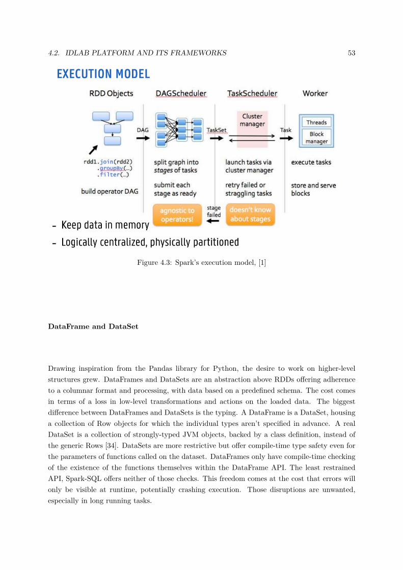
4.2. IDLAB PLATFORM AND ITS FRAMEWORKS 53
Figure 4.3: Spark’s execution model, [1]
DataFrame and DataSet
Drawing inspiration from the Pandas library for Python, the desire to work on higher-levelstructures grew. DataFrames and DataSets are an abstraction above RDDs offering adherenceto a columnar format and processing, with data based on a predefined schema. The cost comesin terms of a loss in low-level transformations and actions on the loaded data. The biggestdifference between DataFrames and DataSets is the typing. A DataFrame is a DataSet, housinga collection of Row objects for which the individual types aren’t specified in advance. A realDataSet is a collection of strongly-typed JVM objects, backed by a class definition, instead ofthe generic Rows [34]. DataSets are more restrictive but offer compile-time type safety even forthe parameters of functions called on the dataset. DataFrames only have compile-time checkingof the existence of the functions themselves within the DataFrame API. The least restrainedAPI, Spark-SQL offers neither of those checks. This freedom comes at the cost that errors willonly be visible at runtime, potentially crashing execution. Those disruptions are unwanted,especially in long running tasks.
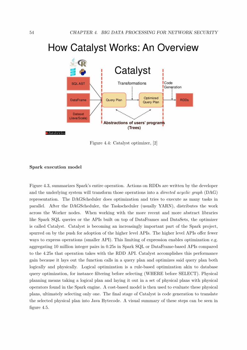
54 CHAPTER 4. BIG DATA PROCESSING FOR NETWORK SECURITY
Figure 4.4: Catalyst optimizer, [2]
Spark execution model
Figure 4.3, summarizes Spark’s entire operation. Actions on RDDs are written by the developerand the underlying system will transform those operations into a directed acyclic graph (DAG)representation. The DAGScheduler does optimization and tries to execute as many tasks inparallel. After the DAGScheduler, the Taskscheduler (usually YARN), distributes the workacross the Worker nodes. When working with the more recent and more abstract librarieslike Spark SQL queries or the APIs built on top of DataFrames and DataSets, the optimizeris called Catalyst. Catalyst is becoming an increasingly important part of the Spark project,spurred on by the push for adoption of the higher level APIs. The higher level APIs offer fewerways to express operations (smaller API). This limiting of expression enables optimization e.g.aggregating 10 million integer pairs in 0.25s in Spark SQL or DataFrame-based APIs comparedto the 4.25s that operation takes with the RDD API. Catalyst accomplishes this performancegain because it lays out the function calls in a query plan and optimizes said query plan bothlogically and physically. Logical optimization is a rule-based optimization akin to databasequery optimization, for instance filtering before selecting (WHERE before SELECT). Physicalplanning means taking a logical plan and laying it out in a set of physical plans with physicaloperators found in the Spark engine. A cost-based model is then used to evaluate these physicalplans, ultimately selecting only one. The final stage of Catalyst is code generation to translatethe selected physical plan into Java Bytecode. A visual summary of these steps can be seen infigure 4.5.
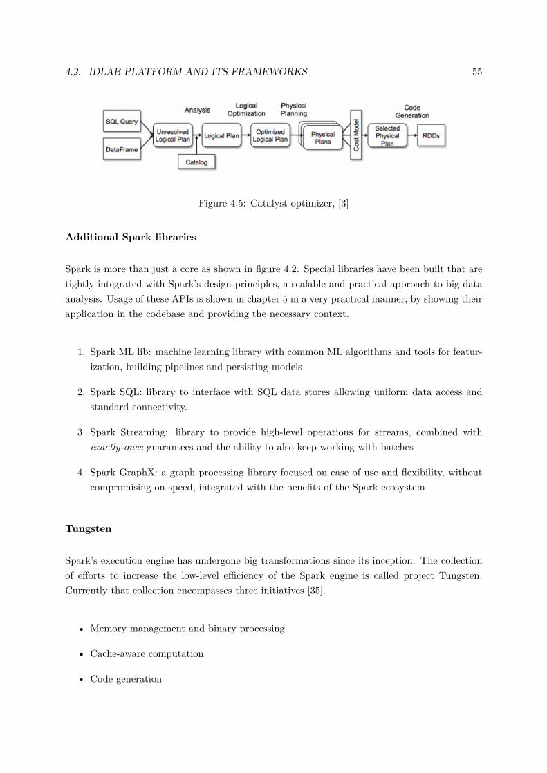
4.2. IDLAB PLATFORM AND ITS FRAMEWORKS 55
Figure 4.5: Catalyst optimizer, [3]
Additional Spark libraries
Spark is more than just a core as shown in figure 4.2. Special libraries have been built that aretightly integrated with Spark’s design principles, a scalable and practical approach to big dataanalysis. Usage of these APIs is shown in chapter 5 in a very practical manner, by showing theirapplication in the codebase and providing the necessary context.
1. Spark ML lib: machine learning library with common ML algorithms and tools for featur-ization, building pipelines and persisting models
2. Spark SQL: library to interface with SQL data stores allowing uniform data access andstandard connectivity.
3. Spark Streaming: library to provide high-level operations for streams, combined withexactly-once guarantees and the ability to also keep working with batches
4. Spark GraphX: a graph processing library focused on ease of use and flexibility, withoutcompromising on speed, integrated with the benefits of the Spark ecosystem
Tungsten
Spark’s execution engine has undergone big transformations since its inception. The collectionof efforts to increase the low-level efficiency of the Spark engine is called project Tungsten.Currently that collection encompasses three initiatives [35].
• Memory management and binary processing
• Cache-aware computation
• Code generation
56 CHAPTER 4. BIG DATA PROCESSING FOR NETWORK SECURITY
The memory aspect aims to eliminate the memory and garbage collector (GC) overhead. Bothissues are tackled by invoking advanced functionality of the JVM that allows explicit, C-stylememory management. The architecture-specific code is Just-In-Time compiled.
Cache-aware computation works towards lifting the in-memory aspect of Spark to new levels,by making effective use of the L1/L2/L3 caches of CPUs. Rewriting algorithms to avoid CPUcache swapping as much as possible, drastically increasing execution speed (e.g. cache-awaresort is 3X faster than the previous cache-unaware method).
The final part of the Tungsten project is code generation. Two key bottlenecks are addressed,first by eliminating polymorphic function dispatching (virtual function calling) and second byimproving serialization for network transport. Polymorphic function dispatching is the methodby which the appropriate functions on objects of classes with inheritance are chosen. Thatprocess of figuring out which method to call on that specific type of object is costly. The secondoptimization involving code generation is serialization. Spark is designed to run in a cluster ofconnected machines. This means that moving data over the wire is a very frequent operation.Increases in performance on the operation of translating back and forth wire protocol and binaryin-memory structure are advantageous across the board.
Conclusion
The previous sections try to give an overview of the Spark project. Starting at the highest levelof abstraction and working down to the optimizations at the level of the Java Virtual Machine(JVM), even going deeper to finish at the improvements on the bare metal.
4.2.2 Apache Kafka
The full layout of the experiment 4.1 has other components besides Apache Spark. Apache Kafkais one of them. It is a distributed streaming platform intended for real-time data pipelines.Speed, horizontal scalability and fault-tolerance are the central goals of Kafka. Because thisthesis isn’t focused on streaming and therefore doesn’t use Apache Kafka, I will only give aminor overview of Kafka’s API.
Kafka has four central APIs [36], the producer API is used to publish (sets of) records in a stream,the consumer API contains functions to handle subscription to those streams, the streaming APIoffers transformations on ingested streams to produce new outgoing ones. Finally the connectorAPI helps to build reusable Kafka endpoints on existing data systems.
A stream of records is called a topic in Kafka. Topics are logical structures, physically they map
4.3. RELATED PLATFORMS 57
onto a distributed collection of partitions, ordered immutable sequences.
For more details about the design principles of Kafka, I’d like to refer to the documentation.
4.2.3 MongoDB
Big data needs distributed, scalable storage. In the streaming experiment setup this storage isdone by MongoDB. Although MongoDB is primarily a JSON store, it can store large files ina binary format called BSON. This is an advantage because Mongo can store both raw packetcapture files and their processed counterparts in JSON (like those exported by Joy). MongoDBincludes a connector for Spark, making integration easy. This research focused on Spark anddidn’t need to use MongoDB for storage. Similar to Apache Kafka only the minimum necessarycontext is given. The MongoDB team puts their product forward as a highly available, scalabledata store. These principles are expressed by the built-in replication and failover as well as nativesharding in MongoDB [37]. So far it has not yet been opportune to integrate with MongoDB,because the research has taken place on a preexisting dataset that can easily be stored on asingle host.
4.3 Related platforms
Other research groups and open source projects exist that focus on the intersection betweenbig data and cyber security. One of these projects BigDAMA has already been described in anearlier section 4.1. The joint project between the Austrian Institute of Technology, TechnicalUniversity of Vienna and the Polytechnic University of Turin, has already published 39 paperssince its inception, a little over two years ago. Those publications are always in the field ofcomputer networking, with special interest for traffic analysis, machine learning and big data,often in the context of security.
The domain registrar for the Dutch national DNS domain (.nl) SIDN has a research arm calledSIDN labs in which it partners with universities including among others the Technical Universityof Delft and the University of Twente. One of the supported research projects is ENTRADA,a High-Performance Network Traffic Data Streaming Warehouse. Entrada [38] converts pcapsof DNS traffic into https://parquet.apache.org/ files after which those get ingested by ApacheImpala, a highly parallel SQL query engine for Hadoop. Apache Spark can be used for morecomplicated forms of analysis.
Another project, which is community-driven and currently incubating as an Apache projectis Spot. Spot other tools of the Apache Project, most notably Apache Spark for the scalable

58 CHAPTER 4. BIG DATA PROCESSING FOR NETWORK SECURITY
machine learning, but also HDFS, YARN, Kafka and others [39]. The full process from ingestionto visualization is covered.
5Machine learning for network security purposes
5.1 Intro
This chapter covers the use of machine learning (ML) as the method of data analysis. A part ofthis chapter is dedicated to the process of becoming familiar with the field of ML, at the datalevel (domain-specific), at the algorithmic level and at the implementation level. It also aimsto indicate the path I have taken as a student who didn’t have any experience in ML beforestarting this dissertation. Conclusions derived from this process are included in the text to serveas documentation about the choices I made and their outcomes. While not entirely relevant forthe technical content of this dissertation, I hope they may prove useful for students in a similarsituation.
59
60 CHAPTER 5. MACHINE LEARNING FOR NETWORK SECURITY PURPOSES
5.2 Data exploration, understanding the problem domain
5.2.1 Different levels of detail
Raw packet capture and flow capture
Network traffic data is high volume, varied data that can be aggregated at different resolutions.The highest resolution network data are full packet captures because they hold all header andpayload information. Zooming out one level brings the data at the flow level, where the individualpackets are no longer visible, but new meta data about the logical connections is kept. Reducingthe resolution even further, means no longer inspecting singular hosts or a collection of hostsinside a subnetwork, but looking at differences between subnetworks. Each step in the hierarchygives new meta data about the collected traffic. The varied nature of network traffic is mostvisible at the packet level. It is due to the plethora of rigorously defined protocols. Meta data atthe packet level is stored in the protocol headers. These are deliberately crafted to contain onlythe necessary information to fulfill the protocol’s requirements. This does mean that every fieldin a header has a distinct set of possible values and associated meaning. Before any attempt athorizontal data reduction, that is selection of relevant headers as features for analysis, can bemade, it is imperative that the working of the protocol itself is well understood. Pure packetdata already has a lot of information to offer, but adding flow data about the same traffic opensup even more options. In theory, packet data should suffice to extract higher level features(flow-level and beyond), but redoing the work to aggregate the packets into logical connections,would be inefficient. For that reason, manufacturers of network hardware support packet andflow based capturing at the hardware level.
Creating context
Packet and flow captures contain detailed information, but may lack in terms of explanationpower of the captured information. Some examples: information like source and destination ad-dress are stored, but they are only numerical representations of network endpoints. Connectionsto endpoints in physical locations, that have shown to carry a higher risk of malicious trafficare not automatically weighted as more dangerous. A similar argument can be made for DNSqueries to known or suspected malicious domains. Only the data associated with the query itselfis stored, not the risk. Temporal information is another form of context that is present in thedata, but not readily available. Unexpected periodicity or off-hour traffic can be a giveawayof malicious activity. A first critique of the introduction of context can be the reliance on lists(which need to be accurate and up-to-date) and a close connection to rule-based intrusion detec-tion systems. In my view these concerns can be dealt with by training other machine learning
5.3. STEPS IN A MACHINE LEARNING SOLUTION 61
models, adapted to a specific task (e.g. malicious URL recognition) supplant simple list check-ing. Those systems would need quality data to learn from, which does mean keeping the listsup-to-date to continuously retrain the models. A second issue with using context, can be thecomputational cost of calculating the feature itself or the cost of calculating a risk score basedon the context of said feature.
Further aggregation
Identification of features at higher levels of abstraction is often left to the network administrators.Data at this resolution quickly becomes the domain of Internet Service Providers (ISP), whichmakes its acquisition harder. Nevertheless I think that there might be relevant data to be foundat this level.
5.2.2 Obtaining quality, unbiased data
The biggest problem I encountered when writing a script to parse the pcap files and extractfeatures from them, was which features to select. The traces I worked with back then, were thefirst captures of APT2, not against Metasploitable because I was still working on the vulnerableVM. The target was another server in the experiment, but due to the lack of running services onthat server, the amount of captured data was so tiny that I didn’t feel it was useful data to learnfrom. In order to get going, I decided to work with a public data set called NSL-KDD. Moreinformation about the content of that data set is in subsection 5.5. An additional complicationwas that I didn’t know if the feature set would lend itself to be processed by machine learningalgorithms in a meaningful way. I had never solved a machine learning problem and didn’t knowwhich processing steps were typically required, nor how they interacted with different types ofdata.
5.3 Steps in a machine learning solution
5.3.1 First projects
I started with entry level tutorial projects like processing the iris flower data set. I had alreadydecided to use Python as the language for this dissertation. I had no previous experience inPython, but knew that Python was easy to learn and a great addition to my existing arsenalof languages. By following Machine learning blogs like Machine Learning Mastery, I was ableto pick up the essential steps of writing machine learning solutions from start to finish. The
62 CHAPTER 5. MACHINE LEARNING FOR NETWORK SECURITY PURPOSES
process can be broken down like this:
• Delimit the problem space, this means mostly to set a heading and trying to understandhow the available data relates to the goal
• Data loading, this means taking the data out of (potentially multiple) data stores
• Data preprocessing, this means molding the data into a form that is processable by theML algorithm. This process potentially has a lot of steps including, but not limited to
– Feature encoding (one-hot encoding, binary encoding, string indexing, ...)
– Feature scaling (normalization, max-min, ...)
– Outlier removal
– Horizontal data reduction = dimensional reduction (selecting high-impact features,removing correlated ones)
– Vertical data reduction (selecting representative samples)
• Evaluate the chosen algorithms, using evaluation metrics like accuracy, precision, recall,time spent, memory requirements, ...
• Parameter optimization and algorithm validation (cross-validation) to improve and stabi-lize the results
• Final model training and model storage
This list is not definitive, some steps may be omitted, others may be added. These choicesdepend on the data being worked with.
My preferred approach to learning these steps in practice, was working through tutorials, anno-tating each step with explanation. The annotated versions are available on the Github of thisdissertation. After acquiring this knowledge, I built my implementations. There are three ofthem and they range from using only pandas and scikit-learn to one with maximal usage of theSpark API. These versions will be discussed later in this text.
5.3.2 Mathematical background, Coursera
I attribute high value to deep understanding of the inner workings of machine learning algorithmsto learn why they exhibit their positive and negative characteristics. To fill in the lack of coursematerial in my curriculum about machine learning / AI, I enrolled in the Coursera MachineLearning course. This course focuses on implementation of machine learning algorithms in
5.4. STATE OF THE ART 63
Octave (a MATLAB dialect), always starting from the relevant mathematical background. Thecourse is created by Stanford University and taught by Andrew Ng, former head of the BaiduAI group and Google Brain. Unfortunately I have had to abandon this course, not because ofthe quality of the content, but because I couldn’t fit the time requirements into my planning.Implementation of machine learning algorithms isn’t the focus of this dissertation and it didn’tprovide enough material immediately applicable to this research. Ideally, I would have had thisknowledge before starting and that’s why I am very keen on picking this course back up afterthis research, in preparation of further research.
5.4 State of the art
In order to get a comprehensive overview, I have read a collection of published material, startingwith survey papers to get a base understanding before proceeding with recent papers proposingnew or improved solutions.
Buczak et al. have written a survey paper about data mining and ML methods for IDS purposes.They give an overview of the process of writing machine learning solutions, network trafficcapture types (packet vs flow) and available public data sets. The bulk of their research isa comparison between the algorithms typically used in intrusion detection. Their comparisonis a.o. based on time complexity, accuracy, understandability of the model and capability ofstreaming [40]. Their research guided me in choosing part of the set of algorithms, which includesk-nearest-neighbors (kNN), decision trees (DTree), random forests (RForest) and support vectormachines (SVM).
Zuech et al. wrote about the application of intrusion detection on big, heterogeneous data.They aim to provide insight in the specific issues arising from both the scale of the problem andthe heterogeneity of the data. In their research they highlight the importance of other sourcesof data that should be included in a detection system, trying to move the research up a levelin terms of abstraction to SIEMs. They conclude that correlation between traditional cybersecurity data and anomalous real-world measurements should be the direction to follow. Thisin an effort to monitor and protect industrial sites and critical infrastructure. [41]
Chandola et al.’s paper ”anomaly detection: a survey” was used to get an introduction into theconcepts, types and challenges of anomalies as well as a listing of the fields for which anomalydetection is studied. Furthermore the paper gives detailed descriptions with advantages anddisadvantages of anomaly detection techniques (like classification, clustering, statistical, a.o.)[42]. This information was very helpful to recognize the different types of anomalies (point,contextual and collective) in network traffic and to make informed decisions on the types ofalgorithmic solutions to adopt.
64 CHAPTER 5. MACHINE LEARNING FOR NETWORK SECURITY PURPOSES
Bhuyan et al. have wrote a review paper classifying other research papers about IDS into anumber of categories, covering more methods and stages than other survey papers of this kind.They give details about the categorization of attacks, a generic architecture for IDS systems,data sets, proximity measures, cluster validity measures and evaluation metrics [43]. Thatinformation is provided to give enough context for a good understanding of the comparisonbetween the methods, invented by other researchers. For my this review paper filled some gapsin my knowledge with regard to the available tools and served as a formulary for proximity andevaluation metrics.
The final review paper by Liao et al. focuses on the different design choices for an IDS system,splitting them across four dimensions [44].
• The detection methodology (rule-based, anomaly-based or protocol analysis)
• The technology type (host-based, wired, wireless and network behavior analysis)
• The attack detection (known, unknown, combination)
• The accuracy
This information served to enhance my understanding of the strengths and weaknesses of eachsystem.
Karimi et al. have written about feature extraction in real-time IDS scenarios by proposingan architecture built on Apache Spark and HDFS that can extract features in near real-time.They used the CAIDA data set which contains the traces of a DDos attack. This research wasinteresting for this dissertation, because it showed that Spark can be used for efficient featureextraction when given enough hardware to scale [45].
Portnoy et al. describe an unsupervised anomaly detection method based on clustering. Theypropose a new clustering algorithm that divides new samples into clusters based on proximityto the existing clusters and cluster width. After training (clustering) a portion of the clustersis labeled normal and the other portion is labeled anomalous. The two parameters to tune forthis model are the cluster width and the percentage of clusters to be labeled as normal. Thetesting was done on the KDD99 data set. After testing they observed that a smaller numberof clusters labeled as normal resulted in higher accuracy, but also higher false positive rate.They also tweaked the cluster width and used the results in a 10-fold cross validation. Thedetection rates varied between 18,56% and 56,25% [46]. My main takeaway for this study wasthat the advantages of using unsupervised methods (no labeling and detection of novel attacks)were overshadowed by the poor classification performance. It should be noted that this researchhappened before the feasibility of neural networks, relying solely on a clustering algorithm.
5.4. STATE OF THE ART 65
Lin et al. introduce a new technique for intrusion detection based on the combination of nearestneighbors and cluster centers (CANN). For a new dataset a clustering technique is used to findthe cluster centers. For the individual data points in the set, their closest neighbors are sought.Then for each sample the distance to its cluster center and its nearest neighbor are summedinto a new metric. This metric replaces all previous metrics for that point and is added to anew dataset. The transformed dataset and the original set are combined and a kNN classifier istrained on that data. The KDD99 data set was used to evaluate this algorithm. CANN provesto reach very similar results to kNN on the same dataset with a selection of 19 features fromKDD99 and outperforms kNN on when the dataset uses only 6 features [47].
Suthaharan et al. explore the problems and challenges introduced by machine learning solutionto the intrusion detection problem. They start their analysis by suggesting a new triplet ofcharacteristics for big data to replace volume, velocity and variety. They suggest using cardinal-ity (number of records), continuity and complexity. Cardinality and continuity mainly impactstorage technologies. The complexity parameter consists of attributes like number of classes,structured vs. unstructured data, dimensionality and requirements in processing speed. Interms of algorithmic improvements they focus on the improvement of SVMs with representationlearning to cope with the big scale. Representation learning transforms the data into anotherdomain, reducing computational complexity to increase processing speed with possible gains inaccuracy as well. The impact of continuity for machine learning is the necessary introduction oflifelong learning systems that need retraining, with partial retention of the previous model [48].This paper was useful to know the problems with machine learning systems in production andhow to alleviate them.
Shon et al. propose an enhanced SVM with three additional techniques to improve the per-formance of their approach. The stages of their solution include using self organizing featuremaps (SOFM) to profile packets. SOFM is a neural network (unsupervised) for dimensional-ity reduction, creating low dimensional (typically 2D) representation of high-dimensional data.The second stage is a packet filter to discard malformed TCP/IP data if it doesn’t come fromwell-written network stack implementations that adhere to the requests for comments (RFC,standards). Third the fields to use as features are selected by a genetic algorithm. The centralmachine learning algorithm is a combination of the soft-margin SVM and the one-class SVM[49]. After testing they conclude that the filtering process filters out about 6% of abnormal pack-ets. The use of a genetic algorithm speeds up the processing and their enhanced SVM has thebenefits of an unsupervised algorithm (not needing labels). Compared to signature-based toolslike Snort and Bro their system was able to pick up novel attacks, but fell behind in detectionof known attacks. This research was interesting to learn how combined methods for intrusiondetection are built and how they improve aspects like accuracy and execution time.
This paragraph concludes the research into the state of the art with regards to machine learning.
66 CHAPTER 5. MACHINE LEARNING FOR NETWORK SECURITY PURPOSES
The survey papers were instrumental in getting a grasp of the scope of the problem. Theindividual papers were useful mostly to see the improvements that can be made when focusingon a single step of the problem and the followed research methodology.
5.5 NSL-KDD
As mentioned in section 5.2.2, working with self-gathered data proved to be difficult. The mainculprits are its lack of attack traffic, lack of labeling and lack of size. The fist two issues are thebiggest hurdles, because a very small sample of real attack traffic offers almost no room to learnwhat features distinguish it from normal traffic, nor is it sufficient to build a generalized modelfrom it. The lack of labeled samples introduces a new problem of having to either label thedata manually or using existing detectors to label the data, relying on their accuracy. Manuallabeling is infeasible because it doesn’t scale and sometimes packets or flows are by themselvesnot anomalous, but are anomalous when put into context. The labeling issue might be avoidedif unsupervised machine learning algorithms are used. This opens a whole new collection ofalgorithms and corresponding background knowledge. Neural networks are definitely a directionto work towards, but one that was not chosen for this thesis because the interpretability of themodel they create is very low.
It is because of these reasons that the choice was made to work with an existing data set calledNSL-KDD. It is an improved version of the KDD99 data set. KDD99 is a data set createdfrom data of the DARPA’98 IDS program. The training set of KDD99 contains approximately4900000 connection records, each consisting of 41 features. The attacks are split across fourcategories discussed in the introduction 1 as the broad types of cyber attacks, DoS, U2R, R2Land probing. The KDD99 data set has basic features taken straight from the meta data ofthe TCP/IP connections. Other features had to be computed for instance in a time interval(traffic features) or based on the payload in the connections (content features). KDD99 hasbeen subjected to criticism, provoking detailed analysis of its quality. It has been discoveredthat KDD99 suffers from redundant records (introducing bias), duplicate records, an overallhigh number of records (forcing researchers to use samples to train in reasonable time, butmaking comparison between runs and other research on the same set difficult) and a difficultyproblem. The difficulty problem lies in the fact that most of the classifiers were all highlycapable of labeling the test and train set properly. This reduces the usability of metrics likeaccuracy to evaluate the algorithms [50]. These deficiencies have led to the creation of animproved data set, called NSL-KDD. It still uses the same features, but removed the redundantand duplicate records, cut down the total size of the data set and solved the difficulty problemby using an inverse sampling method, favoring records that were improperly labeled by a lotof the algorithms. For instance all five detectors labeled the same collection of records with an
5.6. IMPLEMENTATION 67
accuracy of 80%, then only sample 20% of those records for the final dataset. NSL-KDD is animprovement over KDD99, but it too is subject to criticism, mainly that the attack types arealmost 20 years old and no longer representative of modern, low footprint attacks. This criticismencourages the creation of new data sets like UNSW-NB15 [51]. For more information on themeaning of the features in the NSL-KDD dataset, I would like to refer to the appendix of thepaper by Iglesias et al. [52] who did an analysis of relevance of the features in NSL-KDD.
5.6 Implementation
The analysis has been implemented in three different forms. The first is a solution using Pandasfor dataframe operations and scikit-learn for the machine learning classifier. The second solutionreplaces scikit-learn with Spark, but keeps pandas and the custom preprocessing. The third andfinal solution replaces panda and the custom preprocessing in favor of using the Spark API asmuch as possible. The set of algorithms are supervised classification methods. The full listof tested algorithms contains k-nearest neighbors (kNN), linear support vector classifier (linearSVC), decision trees, random forests and a binary logistic regression classifier. I will give a shortdescription of k-nearest neighbors in layman’s terms, but will refer to Bishop [53] and Murphy[54] for a comprehensive reading of all the algorithms. kNN’s working can best be described bymeans of an example. Suppose there are twenty people in a room of which you know the heightand the gender (male / female). K-nearest neighbors will hold this data in-memory. When a21st person walks into the room, we measure the height, but don’t determine the gender. In ascenario where k=3, the three people who are the closest to the 21st person in terms of heightare searched for and selected. The gender of those three people is known and the gender of the21st person is assigned based on the majority gender of those three people. If two of them arefemale, the 21st person is labeled as female or vice versa if two of the three closest are male.In this example the feature dimension is one, because only height was considered to predict thegender. NSL-KDD uses 41 features, some of which are categorical and not directly usable forknn. After one-hot-encoding the number of dimensions shoots up to 122 (one-hot-encoding: 1feature with 9 categorical values, become 9 binary features). A complication to keep in mindis that both supervised (like knn) and unsupervised (like k-means) algorithms which rely on adistance metric (Euclidean, Manhattan, Chebyshev, Minkowsky, ...) become less meaningful inhigh-dimensional space. Iglesias et al. did an analysis of the relevance of the features in theNSL-KDD dataset and concluded that there is a subset of 16 features that contribute the mostto the classification, while others have almost no impact [52]. They propose using the smallerfeature set to do the analysis. Unfortunately two of the three categorical features are still presentin this subset of 16, which after encoding still end up being 95 features in total. I have opted toreduce the feature set of 16 down to 14, eliminating the categorical features.
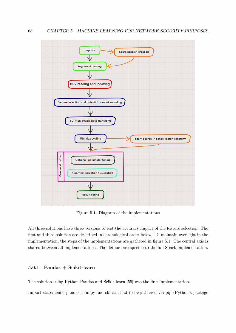
68 CHAPTER 5. MACHINE LEARNING FOR NETWORK SECURITY PURPOSES
Figure 5.1: Diagram of the implementations
All three solutions have three versions to test the accuracy impact of the feature selection. Thefirst and third solution are described in chronological order below. To maintain oversight in theimplementation, the steps of the implementations are gathered in figure 5.1. The central axis isshared between all implementations. The detours are specific to the full Spark implementation.
5.6.1 Pandas + Scikit-learn
The solution using Python Pandas and Scikit-learn [55] was the first implementation.
Import statements, pandas, numpy and sklearn had to be gathered via pip (Python’s package
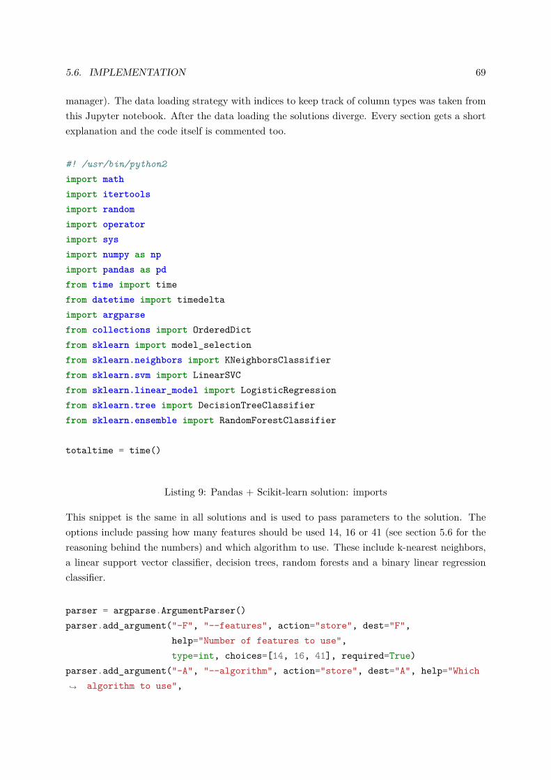
5.6. IMPLEMENTATION 69
manager). The data loading strategy with indices to keep track of column types was taken fromthis Jupyter notebook. After the data loading the solutions diverge. Every section gets a shortexplanation and the code itself is commented too.
#! /usr/bin/python2import mathimport itertoolsimport randomimport operatorimport sysimport numpy as npimport pandas as pdfrom time import timefrom datetime import timedeltaimport argparsefrom collections import OrderedDictfrom sklearn import model_selectionfrom sklearn.neighbors import KNeighborsClassifierfrom sklearn.svm import LinearSVCfrom sklearn.linear_model import LogisticRegressionfrom sklearn.tree import DecisionTreeClassifierfrom sklearn.ensemble import RandomForestClassifier
totaltime = time()
Listing 9: Pandas + Scikit-learn solution: imports
This snippet is the same in all solutions and is used to pass parameters to the solution. Theoptions include passing how many features should be used 14, 16 or 41 (see section 5.6 for thereasoning behind the numbers) and which algorithm to use. These include k-nearest neighbors,a linear support vector classifier, decision trees, random forests and a binary linear regressionclassifier.
parser = argparse.ArgumentParser()parser.add_argument("-F", "--features", action="store", dest="F",
help="Number of features to use",type=int, choices=[14, 16, 41], required=True)
parser.add_argument("-A", "--algorithm", action="store", dest="A", help="Whichalgorithm to use",↪→
70 CHAPTER 5. MACHINE LEARNING FOR NETWORK SECURITY PURPOSES
type=str, choices=["kNN", "DTree", "linSVC", "RForest","binLR"],required=True)
↪→
↪→
results = parser.parse_args()
# 41, 16 or 14 Features# 16 after one hot encoding leads to 95 features# 41 after one hot encoding leads to 122 featuresF = results.FA = results.A
Listing 10: Pandas + Scikit-learn solution: argument parsing
The data set gets loaded from the host’s drive. It isn’t stored in a special filesystem like HDFS orstored in the MongoDB database of the existing experiment because the comma separated value(CSV) file with the dataset is only 14 MB. Every column name is stored in an array to serve asheaders for the dataframe read in by pandas. Column indices are stored and mapped to columnnames to keep track of the different types of features (numerical, categorical and binary). Thisis for future use in data preparation. Sometimes ... shows up in an array or dictionary. Thismeans that a part was omitted to reduce the amount of redundant text.
# Raw datatrain20_nsl_kdd_dataset_path = "NSL_KDD_Dataset/KDDTrain+_20Percent.csv"train_nsl_kdd_dataset_path = "NSL_KDD_Dataset/KDDTrain+.csv"test_nsl_kdd_dataset_path = "NSL_KDD_Dataset/KDDTest+.csv"
# Column namescol_names =
np.array(["duration","protocol_type",...,"labels","labels_numeric"])↪→
# All columns with nominal values (strings)nominal_indexes = [1,2,3]# All columns with binary valuesbinary_indexes = [6,11,13,14,20,21]# All other columns are numeric data, clever way of differencing, create range,
transform it to a set and subtract the other indices, finally convert thatto a list
↪→
↪→
numeric_indexes =list(set(range(41)).difference(nominal_indexes).difference(binary_indexes))↪→
5.6. IMPLEMENTATION 71
# Map the columns types to their name# tolist is non-native python, it is available as a function on numpy ndarrays,
which col_names is↪→
nominal_cols = col_names[nominal_indexes].tolist()binary_cols = col_names[binary_indexes].tolist()numeric_cols = col_names[numeric_indexes].tolist()
dataframe = pd.read_csv(train_nsl_kdd_dataset_path,names=col_names)dataframe = dataframe.drop('labels_numeric',axis=1)
Listing 11: Pandas + Scikit-learn solution: reading CSV and indexing
This code shows the difference in processing steps, depending on the number of features. In thecase of F14 and F16, the list of features to remain is stored and the indices are updated to reflectthe future layout of the dataframe. F16 shares another step with F41 and that is the one-hot(or dummy) encoding of the categorical features plus the removal of the original column. Thecommented display statement is the preferred way to print pandas dataframes in a controlledfashion. Even though the real solution includes this display block several more times to checkthe output of the preprocessing, they have been removed in the snippets, because they don’tadd more meaning.
if F == 14:relevant14 = np.array(['dst_bytes', 'wrong_fragment', ...,
'dst_host_rerror_rate'])↪→
relevant14 = np.append(relevant14, ['labels'])numeric_indexes = list(range(14))numeric_cols = relevant14[numeric_indexes].tolist()dataframe = dataframe[relevant14]
if F == 16:relevant16 = np.array(['service', 'flag', 'dst_bytes',...,
'dst_host_rerror_rate'])↪→
relevant16 = np.append(relevant16, ['labels'])nominal_indexes = [0, 1]numeric_indexes = list(set(range(16)).difference(nominal_indexes))nominal_cols = relevant16[nominal_indexes].tolist()numeric_cols = relevant16[numeric_indexes].tolist()dataframe = dataframe[relevant16]# one hot encoding for categorical featuresfor cat in nominal_cols:
72 CHAPTER 5. MACHINE LEARNING FOR NETWORK SECURITY PURPOSES
one_hot = pd.get_dummies(dataframe[cat])dataframe = dataframe.drop(cat, axis=1)dataframe = dataframe.join(one_hot)
if F == 41:# one hot encoding for categorical features
for cat in nominal_cols:one_hot = pd.get_dummies(dataframe[cat])dataframe = dataframe.drop(cat, axis=1)dataframe = dataframe.join(one_hot)
# with pd.option_context('display.max_rows', 10, 'display.max_columns',None):# print dataframe
Listing 12: Pandas + Scikit-learn solution: feature selection
In the original data set, the attacks are denoted by their names. A mapping is needed totranslate the attacks to their respective categories. The choice was made to work with a twodimensional label, attack (1) or normal (0). An open refinement is a mapping to the broaderattack categories (U2R, R2L, probe, DoS and normal).
# Coarse grained dictionary of the attack types, every packet will be normal oris an attack, without further distinction↪→
attack_dict_coarse = {'normal': 0,
'back': 1,...'udpstorm': 1,
'ipsweep': 1,...'saint': 1,
'ftp_write': 1,...'worm': 1,
'buffer_overflow': 1,...'xterm': 1
5.6. IMPLEMENTATION 73
}
dataframe["labels"] = dataframe["labels"].apply(lambda x:attack_dict_coarse[x])↪→
Listing 13: Pandas + Scikit-learn solution: binarize attack classes
A typical transformation is the normalization of numerical features to reduce their range to afloating point number between 0 and 1. This solution uses min-max scaling instead of standardscore scaling (= (x-avg)/stddev).
# Standardization, formula x-min / max-minfor c in numeric_cols:
mean = dataframe[c].mean()stddev = dataframe[c].std()ma = dataframe[c].max()mi = dataframe[c].min()print c,"mean:",mean,"stddev:",stddev,"max:",ma,"mi:",midataframe[c] = dataframe[c].apply(lambda x: (x-mi)/(ma-mi))
Listing 14: Pandas + Scikit-learn solution: min-max scaling
The location of the labels column is sought to split it from the feature set. This is a necessarystep to feed the data to the classifiers in scikit-learn. Code for cross-validation is custom andperforms a 2/3 train, 1/3 test split with three rounds of validation, each on a different split,guaranteed by the random seed. This code makes calls to individual functions to run the actualML algorithms. Selection of the algorithm is done via the value of the command line argument(stored in A). The functions show which features and their ranges were used to optimize themodels. One example is given in code snippet 16.
label_loc = dataframe.columns.get_loc('labels')array = dataframe.valuesY = array[:,label_loc]X = np.delete(array,label_loc,1)
crossed = {}for cross in range(0, 3):
test_size = 0.33seed = int(round(random.random()*1000000))X_train, X_test, Y_train, Y_test = model_selection.train_test_split(
74 CHAPTER 5. MACHINE LEARNING FOR NETWORK SECURITY PURPOSES
X, Y, test_size=test_size, random_state=seed)data = {
'X_train': X_train,'Y_train': Y_train,'X_test': X_test,'Y_test': Y_test
}if A == 'kNN':
crossed = kNN_with_k_search(data, cross=cross, k_start=1, k_end=51,k_step=2, distance_power=2)↪→
elif A == 'linSVC':crossed = linSVC_with_tol_iter_search(data, cross=cross, tol_start=0,
tol_end=-9, iter_start=0, iter_end=7)↪→
elif A == 'binLR':crossed = binLR_with_tol_iter_search(data, cross=cross, tol_start=0,
tol_end=-9, iter_start=0, iter_end=7)↪→
elif A == 'DTree':crossed = DTree_with_maxFeatures_maxDepth_search(data, cross=cross,
max_depth=30, max_features=F)↪→
elif A == 'RForest':crossed = RForest_with_maxFeatures_maxDepth_search(data, cross=cross,
max_depth=30, max_features=F)↪→
Listing 15: Pandas + Scikit-learn solution: cross-validation
The following two snippets are examples of the methods that have been refactored out of theoriginal solution to streamline it and allow easier extension. The first one is the implementationof kNN with parameter tuning for its single parameter k. The functions for the other algorithmsare very similar in terms of structure. Each one loops over the options for its parameters, buildsa classifier with the options from that iteration, fits a model and scores it on test data. Theresults are stored in a uniform manner in a dictionary which is transformed and sorted later onto show the best model’s outcome after cross-validation.
def kNN_with_k_search(data, cross=0, k_start=1, k_end=101, k_step=2,distance_power=2):↪→
gt0 = time()for k in range(k_start, k_end, k_step):
crossed['knn:k'+repr(k)] = []for k in range(k_start, k_end, k_step):
5.6. IMPLEMENTATION 75
# neat trick to print progress on the same linesys.stdout.write('Round %d, k = %d \r' % (cross, k))sys.stdout.flush()classifier = KNeighborsClassifier(
n_neighbors=k, p=distance_power, n_jobs=-1)classifier.fit(data['X_train'], data['Y_train'])result = classifier.score(data['X_test'], data['Y_test'])crossed['knn:k'+repr(k)].append([result, time()-gt0])
return crossed
Listing 16: Pandas + Scikit-learn solution: kNN parameter tuning
The intention is to find the optimal model parameters with cross-validated testing and to usethose results in a final model with fixed parameters. That’s why each _search function isaccompanied by a _fixed version implementing the algorithm with specific parameters.
def kNN_with_k_fixed(data, k, distance_power):gt0 = time()crossed['knn:k'+repr(k)] = []classifier = KNeighborsClassifier(n_neighbors=k, p=distance_power)classifier.fit(data['X_train'], data['Y_train'])result = classifier.score(data['X_test'], data['Y_test'])crossed['knn:k'+repr(k)].append([result, time()-gt0])return crossed
Listing 17: Pandas + Scikit-learn solution: kNN fixed parameter
This final piece of code uses the dictionary of measures in which k is the key and the values arean array of arrays containing the accuracy and elapsed time. The mean of these measurementsis taken and a single array with the aggregated data replaces the value for k. Finally the top 4results of a sorted version with respect to the accuracy are presented.
for k in crossed:accs = [item[0] for item in crossed[k]]times = [item[1] for item in crossed[k]]crossed[k] = [np.mean(accs), np.std(accs), np.mean(times), np.std(times)]
validated = sorted(crossed.iteritems(), key=lambda (k, v): v[0], reverse=True)for topn in range(0, len(crossed)) if len(crossed) < 5 else range(0, 5):
# validated topn format: avg accuracy, stddev accuracy, avg time,sttdev time↪→
76 CHAPTER 5. MACHINE LEARNING FOR NETWORK SECURITY PURPOSES
print validated[topn]
print('Total time elapsed',str(timedelta(seconds=time()-totaltime)))print('Features',F,'Algorithm',A)
Listing 18: Pandas + Scikit-learn solution: result processing
Even though the Python interpreter itself is single-threaded, setting the n_jobs parameter ofthe KNeighborsClassifier to -1 allows scikit learn to use as many threads as the system has CPUcores. This is essential to be able to compare the performance to Spark’s, which makes use ofparallelism for some of its algorithms. This check has been performed for the other algorithmsas well.
5.6.2 Spark
Chronologically, this is the third solution. There is an intermediate form that only employsSpark for the execution of the ML algorithms. This solution isn’t discussed, but the results inperformance are documented later on. Structurally the solutions with and without Spark areidentical to be able to compare. The full Spark solution makes use of the Spark API wheneverpossible. The import statements already hint at the functionality that Spark provides.
The K-nearest neighbors algorithm isn’t available by default on Spark, but an open sourceimplementation is available on https://github.com/saurfang/spark-knn. Getting the externalmodule to work on the Spark engine was an interesting challenge, especially because the pythonbindings of the project hadn’t been updated to conform to the latest PySpark API (2.3 at thetime of writing). In the process of adapting the Python bindings to the latest version, I learnedthe structure of PySpark and how it is integrated in the Spark project. This knowledge willbe beneficial when debugging other modules, implementing my own distributed algorithms orcreating Python bindings for other modules. My changes to Spark-knn have been merged onthe official module’s Github.
The code also contains a commented line of shell code showing how modules should be linkedto get picked up by Spark.
#! /usr/bin/pythonfrom pyspark import SparkContextfrom pyspark.sql import SparkSessionfrom pyspark.sql.functions import udf, col, min, max, lit, lowerimport pyspark.sql.functions as sqlfrom pyspark.sql.types import *
5.6. IMPLEMENTATION 77
from pyspark.ml.linalg import Vectors, VectorUDT, DenseVectorfrom pyspark.ml import Pipeline, Transformerfrom pyspark.ml.feature import VectorAssembler, StringIndexer,
OneHotEncoderEstimator, MinMaxScaler↪→
from pyspark.ml.tuning import CrossValidator, ParamGridBuilder,TrainValidationSplit↪→
from pyspark.ml.evaluation import BinaryClassificationEvaluatorfrom pyspark_knn.ml.classification import KNNClassifierfrom pyspark.ml.classification import LinearSVC, LogisticRegression,
DecisionTreeClassifier, RandomForestClassifier↪→
from time import timefrom datetime import timedeltaimport numpy as npimport pandas as pdimport randomimport itertoolsimport operatorimport argparseimport math
totaltime = time()
# spark-submit --py-files python/dist/pyspark_knn-0.1-py3.6.egg--driver-class-pathspark-knn-core/target/scala-2.11/spark-knn_2.11-0.0.1-*.jar --jarsspark-knn-core/target/scala-2.11/spark-knn_2.11-0.0.1-*.jar YOUR-SCRIPT.py
↪→
↪→
↪→
Listing 19: Full Spark solution: imports
Spark 2.0 recommends initialization using the method in the code fragment below. Options aregiven to a SparkSession builder to create a session. An important caveat and undocumentedquirk is that config options are ignored when the executor of the script submitted to Spark is theSpark Driver. This was found after investigating numerous crashes of the JVM due to memoryshortage or garbage collection failure. The proper way to set the options is to use the flags forspark-submit. –driver-memory 12g allows the Spark driver to take as much as 12 Gigabytes ofRAM and –num-executors to set the number of CPU cores available. Spark no longer allowspassing memory related options straight to the JVM (like -Xmx for max memory or -Xms forinitial size).
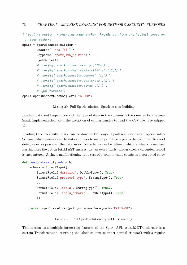
78 CHAPTER 5. MACHINE LEARNING FOR NETWORK SECURITY PURPOSES
# local[*] master, * means as many worker threads as there are logical cores onyour machine↪→
spark = SparkSession.builder \.master('local[*]') \.appName('spark_knn_nslkdd') \.getOrCreate()# .config('spark.driver.memory','12g') \# .config('spark.driver.maxResultSize','10g') \# .config('spark.executor.memory','4g') \# .config('spark.executor.instances','4') \# .config('spark.executor.cores','4') \# .getOrCreate()
spark.sparkContext.setLogLevel("ERROR")
Listing 20: Full Spark solution: Spark session building
Loading data and keeping track of the type of data in the columns is the same as for the non-Spark implementation, with the exception of calling pandas to read the CSV file. See snippet11.
Reading CSV files with Spark can be done in two ways. Spark.read.csv has an option infer-Schema, which passes over the data and tries to match primitive types to the columns. To avoiddoing an extra pass over the data an explicit schema can be defined, which is what’s done here.Furthermore the option FAILFAST ensures that an exception is thrown when a corrupted recordis encountered. A single malfunctioning type cast of a column value counts as a corrupted entry
def read_dataset_typed(path):schema = StructType([
StructField('duration', DoubleType(), True),StructField('protocol_type', StringType(), True),...StructField('labels', StringType(), True),StructField('labels_numeric', DoubleType(), True)])
return spark.read.csv(path,schema=schema,mode='FAILFAST')
Listing 21: Full Spark solution: typed CSV reading
This section uses multiple interesting features of the Spark API. Attack2DTransformer is acustom Transformation, rewriting the labels column as either normal or attack with a regular
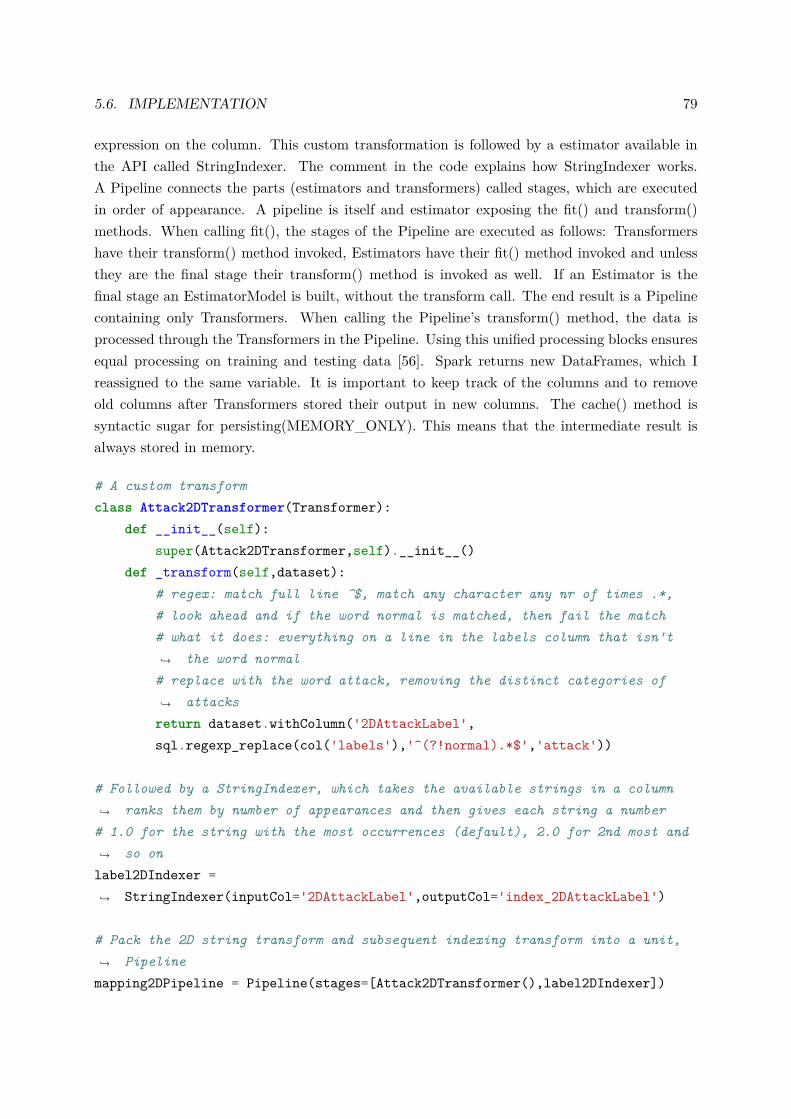
5.6. IMPLEMENTATION 79
expression on the column. This custom transformation is followed by a estimator available inthe API called StringIndexer. The comment in the code explains how StringIndexer works.A Pipeline connects the parts (estimators and transformers) called stages, which are executedin order of appearance. A pipeline is itself and estimator exposing the fit() and transform()methods. When calling fit(), the stages of the Pipeline are executed as follows: Transformershave their transform() method invoked, Estimators have their fit() method invoked and unlessthey are the final stage their transform() method is invoked as well. If an Estimator is thefinal stage an EstimatorModel is built, without the transform call. The end result is a Pipelinecontaining only Transformers. When calling the Pipeline’s transform() method, the data isprocessed through the Transformers in the Pipeline. Using this unified processing blocks ensuresequal processing on training and testing data [56]. Spark returns new DataFrames, which Ireassigned to the same variable. It is important to keep track of the columns and to removeold columns after Transformers stored their output in new columns. The cache() method issyntactic sugar for persisting(MEMORY_ONLY). This means that the intermediate result isalways stored in memory.
# A custom transformclass Attack2DTransformer(Transformer):
def __init__(self):super(Attack2DTransformer,self).__init__()
def _transform(self,dataset):# regex: match full line ^$, match any character any nr of times .*,# look ahead and if the word normal is matched, then fail the match# what it does: everything on a line in the labels column that isn't
the word normal↪→
# replace with the word attack, removing the distinct categories ofattacks↪→
return dataset.withColumn('2DAttackLabel',sql.regexp_replace(col('labels'),'^(?!normal).*$','attack'))
# Followed by a StringIndexer, which takes the available strings in a columnranks them by number of appearances and then gives each string a number↪→
# 1.0 for the string with the most occurrences (default), 2.0 for 2nd most andso on↪→
label2DIndexer =StringIndexer(inputCol='2DAttackLabel',outputCol='index_2DAttackLabel')↪→
# Pack the 2D string transform and subsequent indexing transform into a unit,Pipeline↪→
mapping2DPipeline = Pipeline(stages=[Attack2DTransformer(),label2DIndexer])
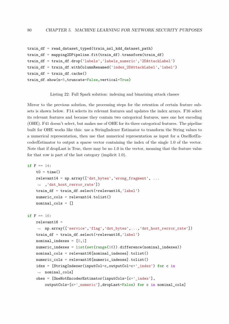
80 CHAPTER 5. MACHINE LEARNING FOR NETWORK SECURITY PURPOSES
train_df = read_dataset_typed(train_nsl_kdd_dataset_path)train_df = mapping2DPipeline.fit(train_df).transform(train_df)train_df = train_df.drop('labels','labels_numeric','2DAttackLabel')train_df = train_df.withColumnRenamed('index_2DAttackLabel','label')train_df = train_df.cache()train_df.show(n=5,truncate=False,vertical=True)
Listing 22: Full Spark solution: indexing and binarizing attack classes
Mirror to the previous solution, the processing steps for the retention of certain feature sub-sets is shown below. F14 selects its relevant features and updates the index arrays. F16 selectits relevant features and because they contain two categorical features, uses one hot encoding(OHE). F41 doesn’t select, but makes use of OHE for its three categorical features. The pipelinebuilt for OHE works like this: use a StringIndexer Estimator to transform the String values toa numerical representation, then use that numerical representation as input for a OneHotEn-coderEstimator to output a sparse vector containing the index of the single 1.0 of the vector.Note that if dropLast is True, there may be no 1.0 in the vector, meaning that the feature valuefor that row is part of the last category (implicit 1.0).
if F == 14:t0 = time()relevant14 = np.array(['dst_bytes','wrong_fragment', ...
,'dst_host_rerror_rate'])↪→
train_df = train_df.select(*relevant14,'label')numeric_cols = relevant14.tolist()nominal_cols = []
if F == 16:relevant16 =
np.array(['service','flag','dst_bytes',...,'dst_host_rerror_rate'])↪→
train_df = train_df.select(*relevant16,'label')nominal_indexes = [0,1]numeric_indexes = list(set(range(16)).difference(nominal_indexes))nominal_cols = relevant16[nominal_indexes].tolist()numeric_cols = relevant16[numeric_indexes].tolist()idxs = [StringIndexer(inputCol=c,outputCol=c+'_index') for c in
nominal_cols]↪→
ohes = [OneHotEncoderEstimator(inputCols=[c+'_index'],outputCols=[c+'_numeric'],dropLast=False) for c in nominal_cols]
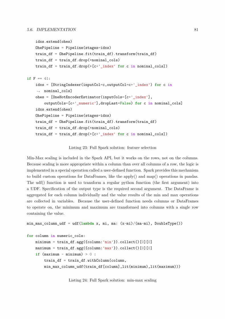
5.6. IMPLEMENTATION 81
idxs.extend(ohes)OhePipeline = Pipeline(stages=idxs)train_df = OhePipeline.fit(train_df).transform(train_df)train_df = train_df.drop(*nominal_cols)train_df = train_df.drop(*[c+'_index' for c in nominal_cols])
if F == 41:idxs = [StringIndexer(inputCol=c,outputCol=c+'_index') for c in
nominal_cols]↪→
ohes = [OneHotEncoderEstimator(inputCols=[c+'_index'],outputCols=[c+'_numeric'],dropLast=False) for c in nominal_cols]
idxs.extend(ohes)OhePipeline = Pipeline(stages=idxs)train_df = OhePipeline.fit(train_df).transform(train_df)train_df = train_df.drop(*nominal_cols)train_df = train_df.drop(*[c+'_index' for c in nominal_cols])
Listing 23: Full Spark solution: feature selection
Min-Max scaling is included in the Spark API, but it works on the rows, not on the columns.Because scaling is more appropriate within a column than over all columns of a row, the logic isimplemented in a special operation called a user-defined function. Spark provides this mechanismto build custom operations for DataFrames, like the apply() and map() operations in pandas.The udf() function is used to transform a regular python function (the first argument) intoa UDF. Specification of the output type is the required second argument. The DataFrame isaggregated for each column individually and the value results of the min and max operationsare collected in variables. Because the user-defined function needs columns or DataFramesto operate on, the minimum and maximum are transformed into columns with a single rowcontaining the value.
min_max_column_udf = udf(lambda x, mi, ma: (x-mi)/(ma-mi), DoubleType())
for column in numeric_cols:minimum = train_df.agg({column:'min'}).collect()[0][0]maximum = train_df.agg({column:'max'}).collect()[0][0]if (maximum - minimum) > 0 :
train_df = train_df.withColumn(column,min_max_column_udf(train_df[column],lit(minimum),lit(maximum)))
Listing 24: Full Spark solution: min-max scaling
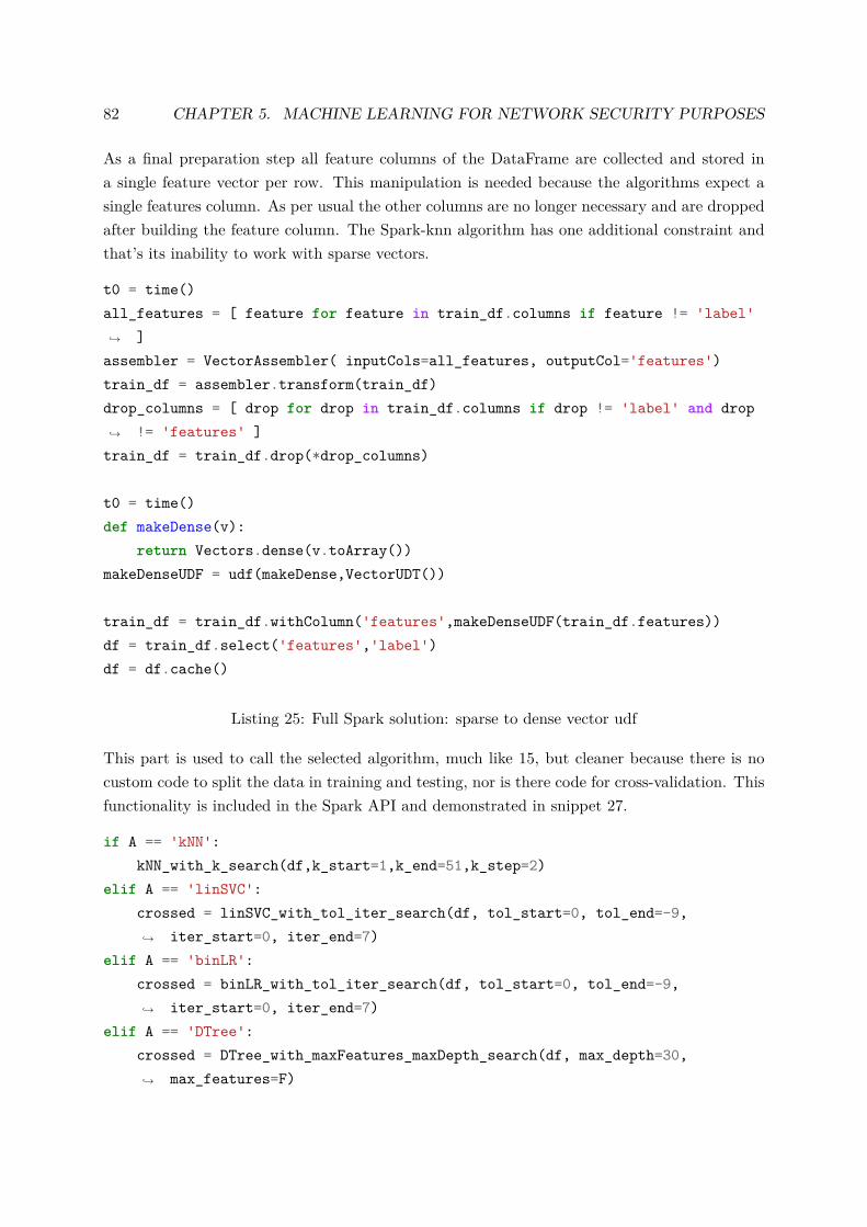
82 CHAPTER 5. MACHINE LEARNING FOR NETWORK SECURITY PURPOSES
As a final preparation step all feature columns of the DataFrame are collected and stored ina single feature vector per row. This manipulation is needed because the algorithms expect asingle features column. As per usual the other columns are no longer necessary and are droppedafter building the feature column. The Spark-knn algorithm has one additional constraint andthat’s its inability to work with sparse vectors.
t0 = time()all_features = [ feature for feature in train_df.columns if feature != 'label'
]↪→
assembler = VectorAssembler( inputCols=all_features, outputCol='features')train_df = assembler.transform(train_df)drop_columns = [ drop for drop in train_df.columns if drop != 'label' and drop
!= 'features' ]↪→
train_df = train_df.drop(*drop_columns)
t0 = time()def makeDense(v):
return Vectors.dense(v.toArray())makeDenseUDF = udf(makeDense,VectorUDT())
train_df = train_df.withColumn('features',makeDenseUDF(train_df.features))df = train_df.select('features','label')df = df.cache()
Listing 25: Full Spark solution: sparse to dense vector udf
This part is used to call the selected algorithm, much like 15, but cleaner because there is nocustom code to split the data in training and testing, nor is there code for cross-validation. Thisfunctionality is included in the Spark API and demonstrated in snippet 27.
if A == 'kNN':kNN_with_k_search(df,k_start=1,k_end=51,k_step=2)
elif A == 'linSVC':crossed = linSVC_with_tol_iter_search(df, tol_start=0, tol_end=-9,
iter_start=0, iter_end=7)↪→
elif A == 'binLR':crossed = binLR_with_tol_iter_search(df, tol_start=0, tol_end=-9,
iter_start=0, iter_end=7)↪→
elif A == 'DTree':crossed = DTree_with_maxFeatures_maxDepth_search(df, max_depth=30,
max_features=F)↪→
5.6. IMPLEMENTATION 83
elif A == 'RForest':crossed = RForest_with_maxFeatures_maxDepth_search(df, max_depth=30,
max_features=F)↪→
print('Total time elapsed',str(timedelta(seconds=time()-totaltime)))print('Features',F,'Algorithm',A)
Listing 26: Full Spark solution: routing logic
This snippet shows the strength of the Spark API, removing the need for custom logic andpackaging a lot of steps in a compact piece. The parameter tuning for the other four algorithmsfollows an identical process. This code is the Spark counterpart to listing 16. First an estimator(knn) is defined with its options, not including the parameter that will be optimized (k). Thena ParamGrid is built using the ParamGridBuilder, specifying the estimator’s parameter valuesto test. An evaluator is added and because the only distinction being made is between normaland attack traffic a BinaryClassificationEvaluator is the right tool. These objects then all serveas parameters for a CrossValidator along with the number of folds and an explicit parallelismsetting. The CrossValidator is an Estimator, which means it outputs a model after calling fit().This model is then evaluated when it is transformed as the argument of the BinaryClassifica-tionEvaluator. The best model after cross-validation is kept and its result and parameter areshown.
def kNN_with_k_search(df, k_start=1, k_end=101, k_step=4):knn = KNNClassifier(featuresCol='features', labelCol='label',topTreeSize=1000, topTreeLeafSize=10, subTreeLeafSize=30)grid =
ParamGridBuilder().addGrid(knn.k,range(k_start,k_end,k_step)).build()↪→
evaluator =BinaryClassificationEvaluator(rawPredictionCol='prediction',labelCol='label')↪→
# BinaryClassificationEvaluator default is areaUnderROC, other option isareaUnderPR↪→
# evaluator.setMetricName('areaUnderROC')cv = CrossValidator(estimator=knn,estimatorParamMaps=grid,
evaluator=evaluator,parallelism=4,numFolds=3)cvModel = cv.fit(df)result = evaluator.evaluate(cvModel.transform(df))print('kNN:k',cvModel.bestModel._java_obj.getK(),result)
Listing 27: Full Spark solution: kNN with cross-validation and parameter tuning
84 CHAPTER 5. MACHINE LEARNING FOR NETWORK SECURITY PURPOSES
For completion and to show one extra part of the Spark API, a function for algorithm evaluationwith fixed parameters is included. TrainValidationSplit is the class in the Spark API for a one-offrandom split of a DataFrame. The other steps are very similar to 27.
def kNN_with_k_fixed(df,k):knn = KNNClassifier(featuresCol='features', labelCol='label',topTreeSize=1000, topTreeLeafSize=10, subTreeLeafSize=30)grid = ParamGridBuilder().addGrid(knn.k,[k]).build()evaluator =
BinaryClassificationEvaluator(rawPredictionCol='prediction',labelCol='label')↪→
tts = TrainValidationSplit(estimator=knn,estimatorParamMaps=grid,evaluator=evaluator,trainRatio=0.6666)
ttsModel = tts.fit(df)result = evaluator.evaluate(ttsModel.transform(df))print('kNN:k',k,result)
Listing 28: Full Spark solution: kNN with fixed parameters
In writing the solutions extensive use was made of the documentation for Apache Spark PythonAPI, Scikit-learn and Pandas. Fluent Python by Luciano Ramalho was consulted to solveproblems related to coding in Python [57].
5.7 Benchmarking and results
Exhaustive testing has been done on all three implementations with special attention for theharmonization of the solutions to optimize comparison quality.
5.7.1 Methodology
Every solution has been tested with all possible combinations of feature counts and algorithmchoices. This resulted in 45 runs, because the three solutions each had three options in termsof feature count and five algorithms to choose from.
Because the accuracy of a model can vary heavily with the choice of its parameters, broadparameter tuning was used to test each algorithm. The results of a single run may not reflecta stable solution, so 3-fold cross validation was performed (2/3-1/3 train-test split) to find thebest average model. The algorithms and their parameter ranges are listed in table 5.1. Someadditional notes for this table are the step counts. In the case of kNN a step of +2 was used.
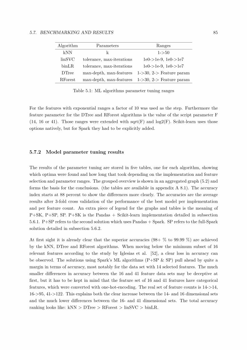
5.7. BENCHMARKING AND RESULTS 85
Algorithm Parameters RangeskNN k 1->50
linSVC tolerance, max-iterations 1e0->1e-9, 1e0->1e7binLR tolerance, max-iterations 1e0->1e-9, 1e0->1e7DTree max-depth, max-features 1->30, 2-> Feature param
RForest max-depth, max-features 1->30, 2-> Feature param
Table 5.1: ML algorithms parameter tuning ranges
For the features with exponential ranges a factor of 10 was used as the step. Furthermore thefeature parameter for the DTree and RForest algorithms is the value of the script parameter F(14, 16 or 41). Those ranges were extended with sqrt(F) and log2(F). Scikit-learn uses thoseoptions natively, but for Spark they had to be explicitly added.
5.7.2 Model parameter tuning results
The results of the parameter tuning are stored in five tables, one for each algorithm, showingwhich optima were found and how long that took depending on the implementation and featureselection and parameter ranges. The grouped overview is shown in an aggregated graph (5.2) andforms the basis for the conclusions. (the tables are available in appendix A 8.1). The accuracyindex starts at 88 percent to show the differences more clearly. The accuracies are the averageresults after 3-fold cross validation of the performance of the best model per implementationand per feature count. An extra piece of legend for the graphs and tables is the meaning ofP+SK, P+SP, SP. P+SK is the Pandas + Scikit-learn implementation detailed in subsection5.6.1. P+SP refers to the second solution which uses Pandas + Spark. SP refers to the full-Sparksolution detailed in subsection 5.6.2.
At first sight it is already clear that the superior accuracies (98+ % to 99.99 %) are achievedby the kNN, DTree and RForest algorithms. When moving below the minimum subset of 16relevant features according to the study by Iglesias et al. [52], a clear loss in accuracy canbe observed. The solutions using Spark’s ML algorithms (P+SP & SP) pull ahead by quite amargin in terms of accuracy, most notably for the data set with 14 selected features. The muchsmaller differences in accuracy between the 16 and 41 feature data sets may be deceptive atfirst, but it has to be kept in mind that the feature set of 16 and 41 features have categoricalfeatures, which were converted with one-hot-encoding. The real set of feature counts is 14->14,16->95, 41->122. This explains both the clear increase between the 14- and 16 dimensional setsand the much lower differences between the 16- and 41 dimensional sets. The total accuracyranking looks like: kNN > DTree > RForest > linSVC > binLR.
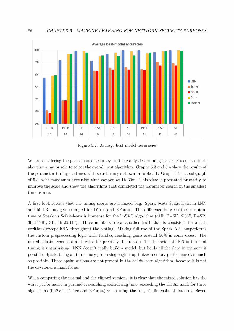
86 CHAPTER 5. MACHINE LEARNING FOR NETWORK SECURITY PURPOSES
Figure 5.2: Average best model accuracies
When considering the performance accuracy isn’t the only determining factor. Execution timesalso play a major role to select the overall best algorithm. Graphs 5.3 and 5.4 show the results ofthe parameter tuning runtimes with search ranges shown in table 5.1. Graph 5.4 is a subgraphof 5.3, with maximum execution time capped at 1h 30m. This view is presented primarily toimprove the scale and show the algorithms that completed the parameter search in the smallesttime frames.
A first look reveals that the timing scores are a mixed bag. Spark beats Scikit-learn in kNNand binLR, but gets trumped for DTree and RForest. The difference between the executiontime of Spark vs Scikit-learn is immense for the linSVC algorithm (41F, P+SK: 2’06”, P+SP:3h 14’48”, SP: 1h 29’11”). These numbers reveal another truth that is consistent for all al-gorithms except kNN throughout the testing. Making full use of the Spark API outperformsthe custom preprocessing logic with Pandas, reaching gains around 50% in some cases. Themixed solution was kept and tested for precisely this reason. The behavior of kNN in terms oftiming is unsurprising. kNN doesn’t really build a model, but holds all the data in memory ifpossible. Spark, being an in-memory processing engine, optimizes memory performance as muchas possible. Those optimizations are not present in the Scikit-learn algorithm, because it is notthe developer’s main focus.
When comparing the normal and the clipped versions, it is clear that the mixed solution has theworst performance in parameter searching considering time, exceeding the 1h30m mark for threealgorithms (linSVC, DTree and RForest) when using the full, 41 dimensional data set. Seven
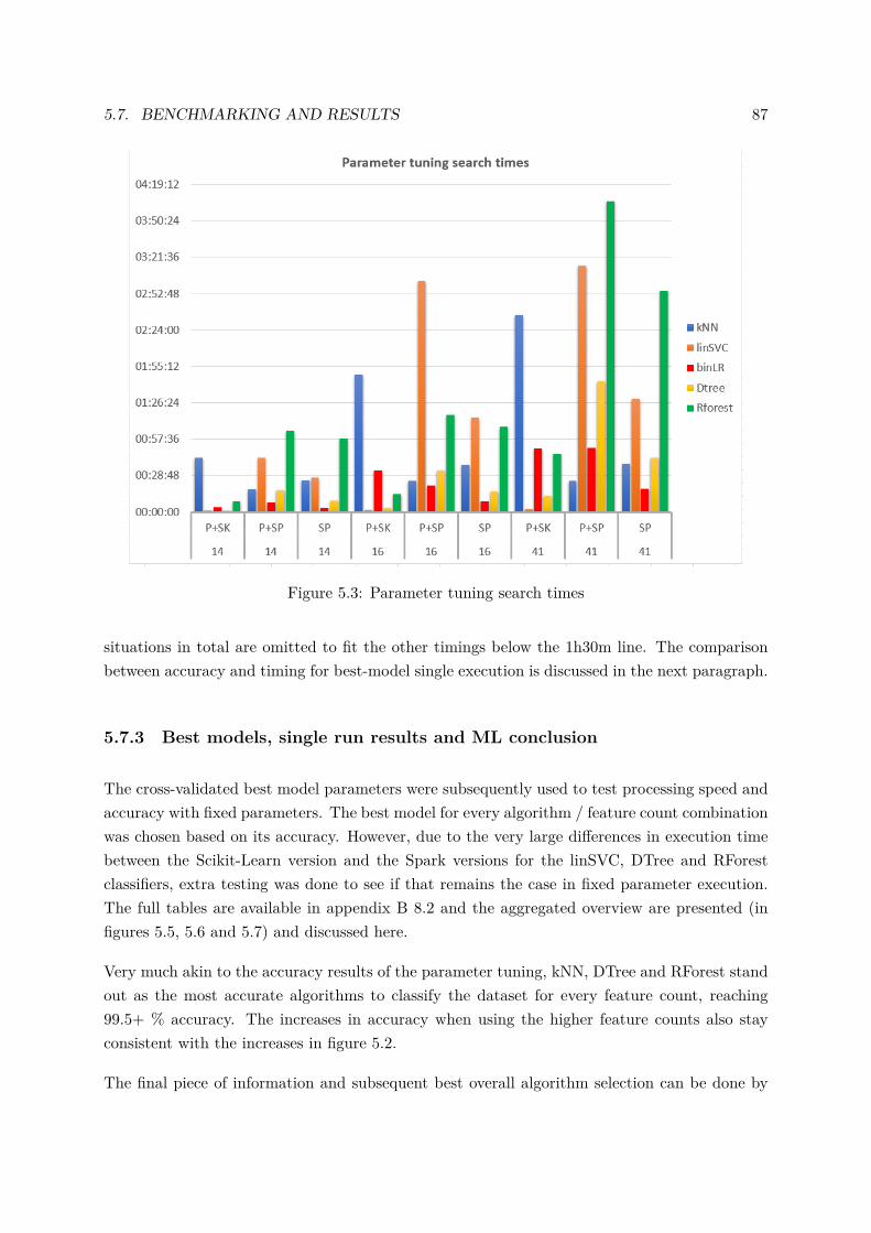
5.7. BENCHMARKING AND RESULTS 87
Figure 5.3: Parameter tuning search times
situations in total are omitted to fit the other timings below the 1h30m line. The comparisonbetween accuracy and timing for best-model single execution is discussed in the next paragraph.
5.7.3 Best models, single run results and ML conclusion
The cross-validated best model parameters were subsequently used to test processing speed andaccuracy with fixed parameters. The best model for every algorithm / feature count combinationwas chosen based on its accuracy. However, due to the very large differences in execution timebetween the Scikit-Learn version and the Spark versions for the linSVC, DTree and RForestclassifiers, extra testing was done to see if that remains the case in fixed parameter execution.The full tables are available in appendix B 8.2 and the aggregated overview are presented (infigures 5.5, 5.6 and 5.7) and discussed here.
Very much akin to the accuracy results of the parameter tuning, kNN, DTree and RForest standout as the most accurate algorithms to classify the dataset for every feature count, reaching99.5+ % accuracy. The increases in accuracy when using the higher feature counts also stayconsistent with the increases in figure 5.2.
The final piece of information and subsequent best overall algorithm selection can be done by
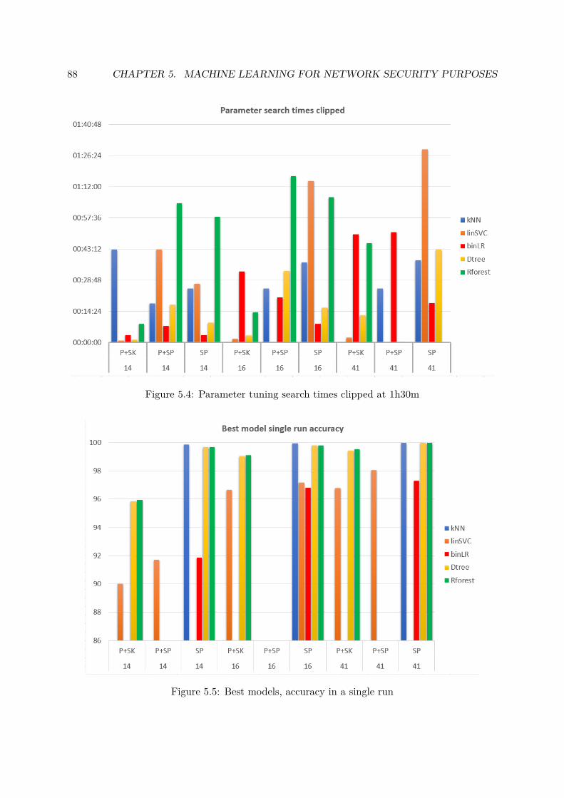
88 CHAPTER 5. MACHINE LEARNING FOR NETWORK SECURITY PURPOSES
Figure 5.4: Parameter tuning search times clipped at 1h30m
Figure 5.5: Best models, accuracy in a single run
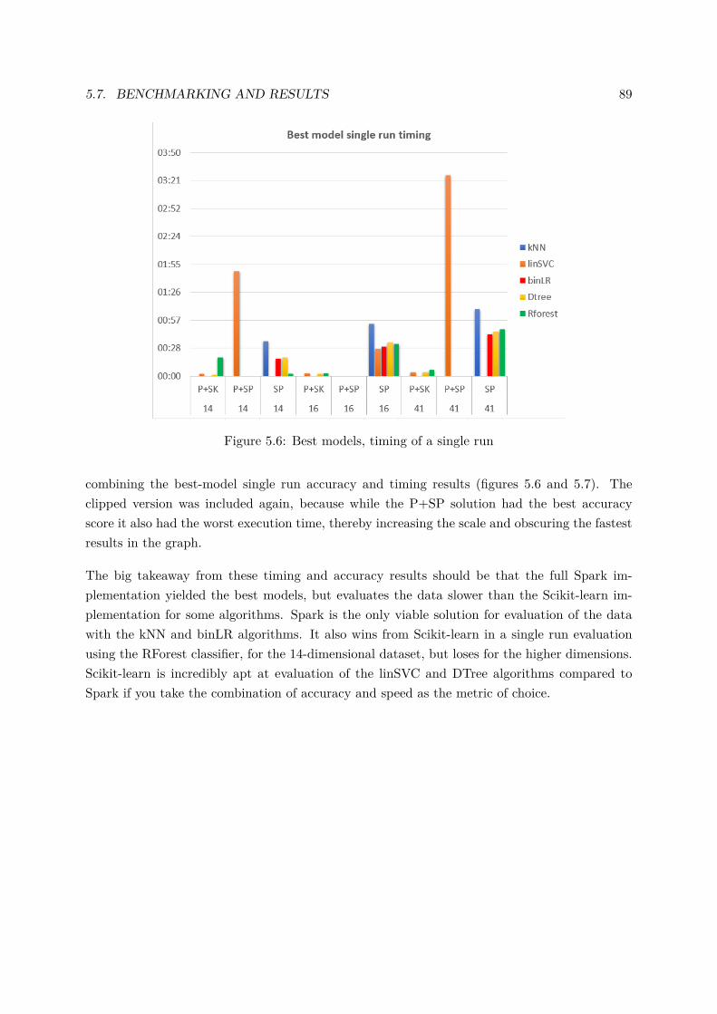
5.7. BENCHMARKING AND RESULTS 89
Figure 5.6: Best models, timing of a single run
combining the best-model single run accuracy and timing results (figures 5.6 and 5.7). Theclipped version was included again, because while the P+SP solution had the best accuracyscore it also had the worst execution time, thereby increasing the scale and obscuring the fastestresults in the graph.
The big takeaway from these timing and accuracy results should be that the full Spark im-plementation yielded the best models, but evaluates the data slower than the Scikit-learn im-plementation for some algorithms. Spark is the only viable solution for evaluation of the datawith the kNN and binLR algorithms. It also wins from Scikit-learn in a single run evaluationusing the RForest classifier, for the 14-dimensional dataset, but loses for the higher dimensions.Scikit-learn is incredibly apt at evaluation of the linSVC and DTree algorithms compared toSpark if you take the combination of accuracy and speed as the metric of choice.
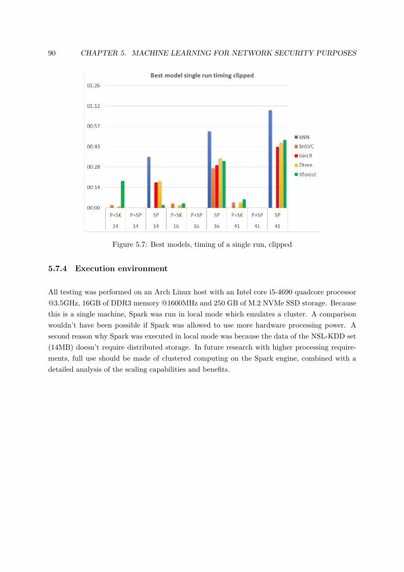
90 CHAPTER 5. MACHINE LEARNING FOR NETWORK SECURITY PURPOSES
Figure 5.7: Best models, timing of a single run, clipped
5.7.4 Execution environment
All testing was performed on an Arch Linux host with an Intel core i5-4690 quadcore [email protected], 16GB of DDR3 memory @1600MHz and 250 GB of M.2 NVMe SSD storage. Becausethis is a single machine, Spark was run in local mode which emulates a cluster. A comparisonwouldn’t have been possible if Spark was allowed to use more hardware processing power. Asecond reason why Spark was executed in local mode was because the data of the NSL-KDD set(14MB) doesn’t require distributed storage. In future research with higher processing require-ments, full use should be made of clustered computing on the Spark engine, combined with adetailed analysis of the scaling capabilities and benefits.

6Future work
Researching this area has opened up a host of options for future work. This chapter sets outdirections for the various parts. The items are listed in no particular order. Because this researchtouches on multiple academic domains, lots of avenues for deeper investigation are open. Thosethat stand out the most to me are written here in a short format.
6.1 Building a data set
Developing a methodology for creating a dataset with modern attack traffic is a goal in andof itself. The introduction of an automated attacker and intentionally vulnerable target in thisdissertation are a great starting point, but leave lots of room for other services, other devicesand other exploits. Introducing those, automated like the current solution, would be very useful(described in more detail in 3.4).
Other challenges in building a data set are:
• Labeling strategy (manual versus using existing classifiers versus no labeling)
• Feature analysis including context- and time-dependent features
• Obtaining diverse baseline data
91
92 CHAPTER 6. FUTURE WORK
6.2 Working with different data sets
This research used the NSL-KDD dataset, but there are other public datasets available, some ofwhich have been described in 5.5. Modifying this solution for use with a more modern datasetand testing how well it performs, would be the method of choice.
6.3 More ML algorithms
This dissertation only makes use of five supervised classification algorithms. The selection isbut a small part of the entire range of possible algorithms. The performance of other importantmachine learning classes and algorithms is an obvious future research path.
• Supervised: neural networks (specifically multilayer perceptrons)
• Unsupervised: particularly other neural nets and clustering algorithms
• Bagging, boosting and stacking impact on ML IDS systems
6.4 User profile integration
Integrating into the existing experiment to close the circuit, offering both streaming- and batchanalysis. Triggered periodically and by anomalies caught in the streaming part to look deeperinto a specific user.
6.5 Big data performance and scaling
• Migrating to Scala to benefit of Spark’s true strength.
• Cluster managers (e.g. Hadoop YARN, Apache Mesos, Spark standalone) and clustertuning
• Testing storage systems, different (types of) databases and file formats

6.6. EXPLORATION OF MULTI-MODEL ARCHITECTURES 93
6.6 Exploration of multi-model architectures
Tailoring detection systems to specific protocols and integrating them into a hierarchy of detec-tors, each contributing to a final score.
7Conclusion
This dissertation at the intersection of network security, big data and machine learning hasexplored each domain in detail, yielding the following set of results and conclusions.
In order to study and improve intrusion detection systems, a high-quality data set is required,preferably labeled. High-quality entails a balanced mix of normal and attack traffic, with featuresthat have a genuine impact on the classification. In addition to not having redundant features,no redundant samples should be present in the set. Gathering attack traffic in a controlledenvironment is challenging and relying on existing detectors undercuts the end goal. In order tofacilitate the capture and labeling of attack traffic with minimal noise, an experiment setup hasbeen built with an automated hacker and intentionally vulnerable target. The attacker buildson a project using Metasploit and nmap automation in Python, with an extensible design. Thevulnerable target is a portable virtual machine, called Metasploitable. The target’s architecturealso encourages extending it with more vulnerable services. The experiment setup combinesthese systems in a layout on Ghent University’s Virtual Wall simulation environment. Packetand flow capture tests of the experiment verified its working and usability.
Network traffic maps directly onto the three dimensions of big data, volume, velocity and variety.Because of this, a part of the research time was invested in getting to the state-of-the artof big data processing, with the specific purpose of network intrusion detection. After thisresearch phase, the Apache Spark engine was studied from an architectural overview down to
94
95
the optimization efforts at the byte- and native code level.
The knowledge from studying Apache Spark in detail was instrumental to the implementationof a machine learning system for network intrusion detection. The state of the art in machinelearning was investigated, both generally, through a selection of review papers and afterwardswith a focus on research specifically about machine learning for network anomaly detection.After acquiring sufficient knowledge, three machine learning solutions were implemented toprocess the public NSL-KDD data set. The three versions are mirrors of each other in termsof structure, but vary in the technologies they use. One uses Pandas and custom code for dataprocessing with Scikit-learn to run the algorithms. The second one uses the same data processingcode, but replaces Scikit-Learn with the Spark API, only for the algorithm execution. Thethird and final implementation drops Pandas in favor of maximal usage of Spark’s capabilities.Five supervised classification algorithms were selected: k-nearest neighbors, a linear supportvector classifier, decision trees, random forests and a binary logistic regression. Each solutionwas further evaluated for reduced sets of features of the NSL-KDD data set, as suggested byresearch.
After broad testing with parameter tuning and cross-validation, average best-fit models wereselected and individually retested to obtain the final results with regards to accuracy and execu-tion time. Processing of the results revealed that the full Spark implementation yielded the mostaccurate models, but paid for that with an increase execution time for some of the algorithms,compared to Scikit-Learn. The Pandas + Scikit-Learn implementation was the undisputed win-ner for the linear support vector and decision tree classifiers, when considering the trade-offbetween speed and accuracy. One other interesting finding was that making maximal use of theSpark API is beneficial compared to writing custom logic for data processing, especially for theexecution time.
The final conclusion of the machine learning research is that big data processing with Spark isa good direction for intrusion detection systems, but attention has to be given to the selectionof algorithms, particularly if execution speed is the primary concern.
Bibliography
[1] P. Simoens, “Deriving data,” in Systeemontwerp, 2017, ch. Deriving data.
[2] D. s. e. Yin Huai, “A deep dive into spark sql’s catalyst optimizer with yin huai.”[Online]. Available: https://www.slideshare.net/databricks/a-deep-dive-into-spark-sqls-catalyst-optimizer-with-yin-huai
[3] M. Armbrust, R. S. Xin, C. Lian, Y. Huai, D. Liu, J. K. Bradley, X. Meng, T. Kaftan, M. J.Franklin, A. Ghodsi, and M. Zaharia, “Spark sql: Relational data processing in spark,” inProceedings of the 2015 ACM SIGMOD International Conference on Management of Data,ser. SIGMOD ’15. New York, NY, USA: ACM, 2015, pp. 1383–1394. [Online]. Available:http://doi.acm.org/10.1145/2723372.2742797
[4] B. J. A. S. L. blog, “The worst data breaches of the last 10 years.” [Online]. Available:https://www.asecurelife.com/the-worst-data-breaches-of-the-last-10-years/
[5] H. project, “What is apache hadoop.” [Online]. Available: http://hadoop.apache.org/#What+Is+Apache+Hadoop%3F
[6] S. Project, “Storm api.” [Online]. Available: http://storm.apache.org/about/simple-api.html
[7] T. E. blog, “Flying faster with twitter heron.” [Online]. Available: https://blog.twitter.com/engineering/en_us/a/2015/flying-faster-with-twitter-heron.html
[8] S. Project, “What is samza.” [Online]. Available: samza.apache.org
[9] CNET, “Hadoop breaks data sorting world records.” [Online]. Available: https://www.cnet.com/news/hadoop-breaks-data-sorting-world-records/
[10] F. Project, “Introduction to apache flink.” [Online]. Available: https://flink.apache.org/introduction.html
[11] S. Chintapalli, D. Dagit, B. Evans, R. Farivar, T. Graves, M. Holderbaugh, Z. Liu, K. Nus-baum, K. Patil, B. J. Peng, and P. Poulosky, “Benchmarking streaming computation en-
96
BIBLIOGRAPHY 97
gines: Storm, flink and spark streaming,” in 2016 IEEE International Parallel and Dis-tributed Processing Symposium Workshops (IPDPSW), May 2016, pp. 1789–1792.
[12] M. Antonakakis, T. April, M. Bailey, M. Bernhard, E. Bursztein, J. Cochran,Z. Durumeric, J. A. Halderman, L. Invernizzi, M. Kallitsis, D. Kumar, C. Lever,Z. Ma, J. Mason, D. Menscher, C. Seaman, N. Sullivan, K. Thomas, and Y. Zhou,“Understanding the mirai botnet,” in Proceedings of the 26th USENIX Security Symposium,2017. [Online]. Available: https://www.usenix.org/conference/usenixsecurity17/technical-sessions/presentation/antonakakis
[13] T. analysis of the Domain Name System (DNS). [Online]. Available: https://tools.ietf.org/html/rfc3833
[14] M. Kührer, T. Hupperich, C. Rossow, and T. Holz, “Exit from hell? reducing the impactof amplification ddos attacks.” in USENIX Security Symposium, 2014, pp. 111–125.
[15] S. T. Zargar, J. Joshi, and D. Tipper, “A survey of defense mechanisms against distributeddenial of service (ddos) flooding attacks,” IEEE communications surveys & tutorials, vol. 15,no. 4, pp. 2046–2069, 2013.
[16] Netcraft, “April 2018 web server survey.” [Online]. Available: https://news.netcraft.com/archives/2018/04/26/april-2018-web-server-survey.html
[17] A. Bittau, A. Belay, A. Mashtizadeh, D. Mazières, and D. Boneh, “Hacking blind,” in 2014IEEE Symposium on Security and Privacy, May 2014, pp. 227–242.
[18] G. Kim, S. Lee, and S. Kim, “A novel hybrid intrusion detection methodintegrating anomaly detection with misuse detection,” Expert Systems with Applications,vol. 41, no. 4, Part 2, pp. 1690 – 1700, 2014. [Online]. Available: http://www.sciencedirect.com/science/article/pii/S0957417413006878
[19] O. Security, “Metsaploit unleashed.” [Online]. Available: https://www.offensive-security.com/metasploit-unleashed/about-meterpreter/
[20] M. project, “Metasploit exploit db.” [Online]. Available: https://www.rapid7.com/db/modules/
[21] T. O’Connor, Violent Python: A Cookbook for Hackers, Forensic Analysts, PenetrationTesters and Security Engineers, 1st ed. Syngress Publishing, 2013.
[22] Rapid7, “Metasploitable3, vulnerable vm.” [Online]. Available: https://github.com/rapid7/metasploitable3
[23] C. systems, “Joy, netflow securit monitoring.” [Online]. Available: https://github.com/cisco/joy
98 BIBLIOGRAPHY
[24] N. project, “Port scanning techniques.” [Online]. Available: https://nmap.org/book/man-port-scanning-techniques.html
[25] A. Fahad, N. Alshatri, Z. Tari, A. Alamri, I. Khalil, A. Y. Zomaya, S. Foufou, and A. Bouras,“A survey of clustering algorithms for big data: Taxonomy and empirical analysis,” IEEETransactions on Emerging Topics in Computing, vol. 2, no. 3, pp. 267–279, Sept 2014.
[26] L. Rettig, M. Khayati, P. Cudré-Mauroux, and M. Piórkowski, “Online anomaly detectionover big data streams,” in 2015 IEEE International Conference on Big Data (Big Data),Oct 2015, pp. 1113–1122.
[27] T. Chen, X. Zhang, S. Jin, and O. Kim, “Efficient classification using parallel and scalablecompressed model and its application on intrusion detection,” vol. 41, p. 5972–5983, 102014.
[28] D. S. Terzi, R. Terzi, and S. Sagiroglu, “Big data analytics for network anomaly detectionfrom netflow data,” in 2017 International Conference on Computer Science and Engineering(UBMK), Oct 2017, pp. 592–597.
[29] A. I. Rana, G. Estrada, M. Solé, and V. Muntés, “Anomaly detection guidelines for datastreams in big data,” in 2016 3rd International Conference on Soft Computing MachineIntelligence (ISCMI), Nov 2016, pp. 94–98.
[30] P. Casas, F. Soro, J. Vanerio, G. Settanni, and A. D’Alconzo, “Network security andanomaly detection with big-dama, a big data analytics framework,” in 2017 IEEE 6thInternational Conference on Cloud Networking (CloudNet), Sept 2017, pp. 1–7.
[31] B. V. Andrés F Ocampo, Tim Wauters and F. D. Turck, “Scalable distributed traffic mon-itoring for enterprise networks with Spark Streaming,” 2017.
[32] S. benchmark, “Gray sort top results.” [Online]. Available: http://sortbenchmark.org/
[33] D. engineering blog, “Apache spark officially sets a new record in large-scale sorting.”[Online]. Available: https://databricks.com/blog/2014/11/05/spark-officially-sets-a-new-record-in-large-scale-sorting.html
[34] ——, “A tale of three apache spark apis: Rdds, dataframes, and datasets.” [On-line]. Available: https://databricks.com/blog/2016/07/14/a-tale-of-three-apache-spark-apis-rdds-dataframes-and-datasets.html
[35] ——, “Project tungsten: brining apache spark close to bare metal.” [Online]. Avail-able: https://databricks.com/blog/2015/04/28/project-tungsten-bringing-spark-closer-to-bare-metal.html
[36] A. K. Project, “Introduction to apache kafka.” [Online]. Available: https://kafka.apache.org/intro
BIBLIOGRAPHY 99
[37] M. Project, “What is mongodb.” [Online]. Available: https://www.mongodb.com/what-is-mongodb
[38] Maarten Wullink, Giovane C. M. Moura, Muller, M, and Cristian Hesselman, “ENTRADA:a High Performance Network Traffic Data Streaming Warehouse,” in Network Operationsand Management Symposium (NOMS), 2016 IEEE (to appear), April 2016.
[39] S. Project, “Apache spot.” [Online]. Available: http://spot.incubator.apache.org/
[40] A. L. Buczak and E. Guven, “A survey of data mining and machine learning methods forcyber security intrusion detection,” IEEE Communications Surveys Tutorials, vol. 18, no. 2,pp. 1153–1176, Secondquarter 2016.
[41] R. Zuech, T. M. Khoshgoftaar, and R. Wald, “Intrusion detection and big heterogeneousdata: a survey,” Journal of Big Data, vol. 2, no. 1, p. 3, Feb 2015. [Online]. Available:https://doi.org/10.1186/s40537-015-0013-4
[42] V. Chandola, A. Banerjee, and V. Kumar, “Anomaly detection: A survey,”ACM Comput. Surv., vol. 41, no. 3, pp. 15:1–15:58, Jul. 2009. [Online]. Available:http://doi.acm.org/10.1145/1541880.1541882
[43] M. H. Bhuyan, D. K. Bhattacharyya, and J. K. Kalita, “Network anomaly detection:Methods, systems and tools,” IEEE Communications Surveys Tutorials, vol. 16, no. 1,pp. 303–336, First 2014.
[44] H.-J. Liao, C.-H. Richard Lin, Y.-C. Lin, and K.-Y. Tung, “Review: Intrusion detectionsystem: A comprehensive review,” J. Netw. Comput. Appl., vol. 36, no. 1, pp. 16–24, Jan.2013. [Online]. Available: http://dx.doi.org/10.1016/j.jnca.2012.09.004
[45] A. M. Karimi, Q. Niyaz, W. Sun, A. Y. Javaid, and V. K. Devabhaktuni, “Distributed net-work traffic feature extraction for a real-time ids,” in 2016 IEEE International Conferenceon Electro Information Technology (EIT), May 2016, pp. 0522–0526.
[46] L. Portnoy, E. Eskin, and S. Stolfo, “Intrusion detection with unlabeled data using cluster-ing,” 11 2001.
[47] W.-C. Lin, S.-W. Ke, and C.-F. Tsai, “Cann: An intrusion detection system based oncombining cluster centers and nearest neighbors,” vol. 78, 01 2015.
[48] S. Suthaharan, “Big data classification: Problems and challenges in network intrusionprediction with machine learning,” SIGMETRICS Perform. Eval. Rev., vol. 41, no. 4, pp.70–73, Apr. 2014. [Online]. Available: http://doi.acm.org/10.1145/2627534.2627557
[49] T. Shon and J. Moon, “A hybrid machine learning approach to network anomalydetection,” Inf. Sci., vol. 177, no. 18, pp. 3799–3821, Sep. 2007. [Online]. Available:http://dx.doi.org/10.1016/j.ins.2007.03.025
100 BIBLIOGRAPHY
[50] M. Tavallaee, E. Bagheri, W. Lu, and A. A. Ghorbani, “A detailed analysis of the kdd cup99 data set,” in Computational Intelligence for Security and Defense Applications, 2009.CISDA 2009. IEEE Symposium on. IEEE, 2009, pp. 1–6.
[51] N. Moustafa and J. Slay, “Unsw-nb15: a comprehensive data set for network intrusion detec-tion systems (unsw-nb15 network data set),” in Military Communications and InformationSystems Conference (MilCIS), 2015. IEEE, 2015, pp. 1–6.
[52] F. Iglesias and T. Zseby, “Analysis of network traffic features for anomaly detection,”Machine Learning, vol. 101, no. 1, pp. 59–84, Oct 2015. [Online]. Available:https://doi.org/10.1007/s10994-014-5473-9
[53] C. M. Bishop, Pattern Recognition and Machine Learning (Information Science and Statis-tics). Berlin, Heidelberg: Springer-Verlag, 2006.
[54] K. P. Murphy, Machine Learning: A Probabilistic Perspective. The MIT Press, 2012.
[55] F. Pedregosa, G. Varoquaux, A. Gramfort, V. Michel, B. Thirion, O. Grisel, M. Blon-del, P. Prettenhofer, R. Weiss, V. Dubourg, J. Vanderplas, A. Passos, D. Cournapeau,M. Brucher, M. Perrot, and E. Duchesnay, “Scikit-learn: Machine learning in Python,”Journal of Machine Learning Research, vol. 12, pp. 2825–2830, 2011.
[56] S. Project, “Pipelines in apache spark.” [Online]. Available: https://spark.apache.org/docs/latest/ml-pipeline.html#pipeline
[57] L. Ramalho, Fluent Python, 1st ed. O’Reilly Media, Inc., 2015.
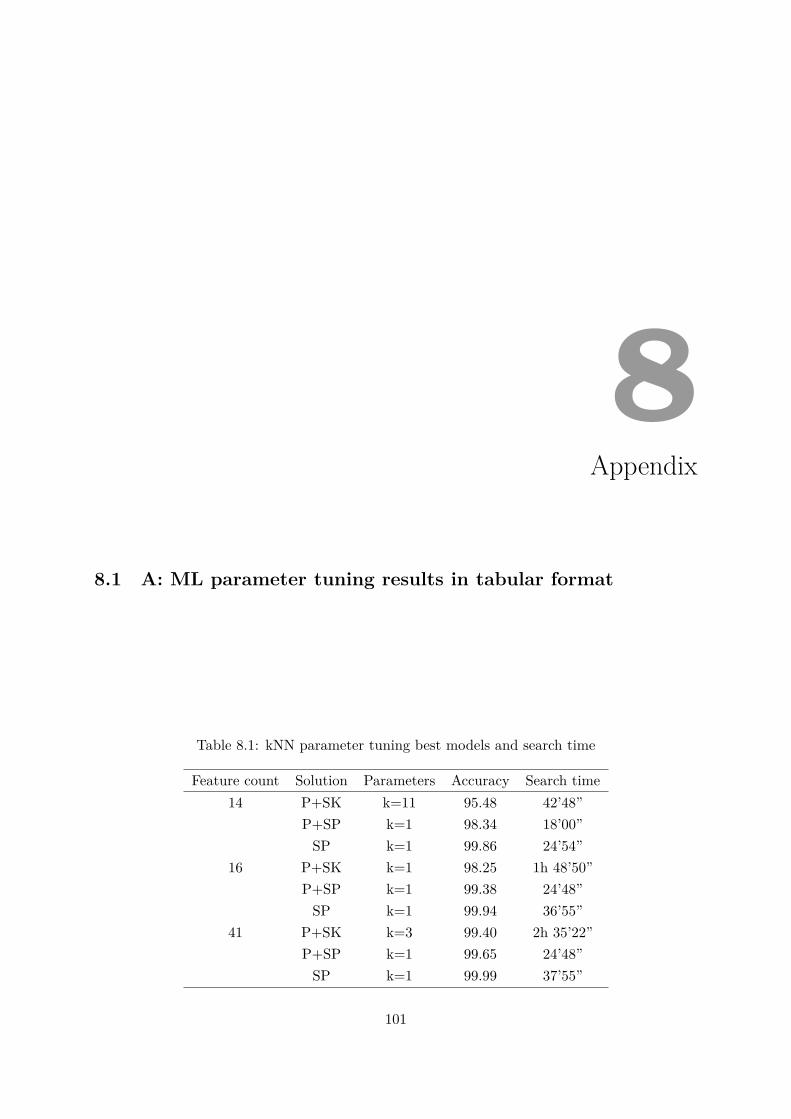
8Appendix
8.1 A: ML parameter tuning results in tabular format
Table 8.1: kNN parameter tuning best models and search time
Feature count Solution Parameters Accuracy Search time14 P+SK k=11 95.48 42’48”
P+SP k=1 98.34 18’00”SP k=1 99.86 24’54”
16 P+SK k=1 98.25 1h 48’50”P+SP k=1 99.38 24’48”
SP k=1 99.94 36’55”41 P+SK k=3 99.40 2h 35’22”
P+SP k=1 99.65 24’48”SP k=1 99.99 37’55”
101
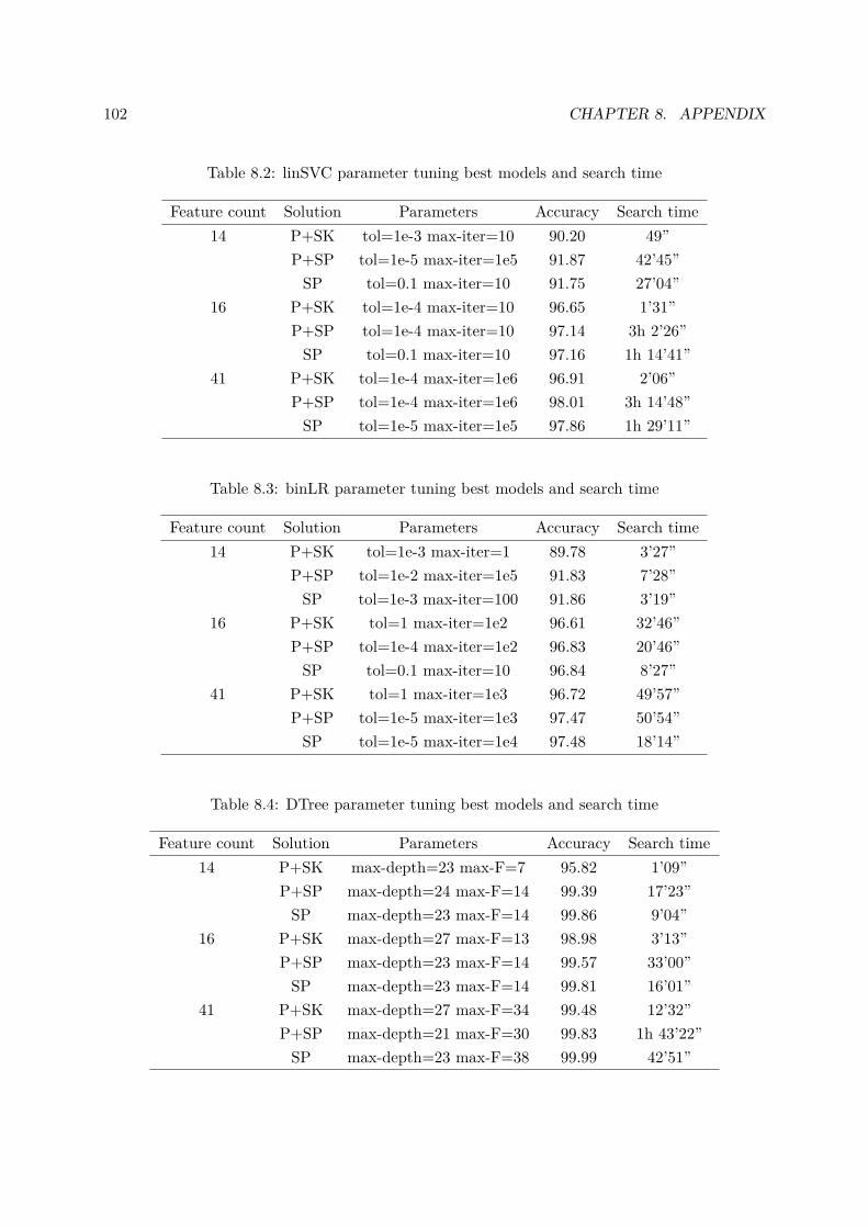
102 CHAPTER 8. APPENDIX
Table 8.2: linSVC parameter tuning best models and search time
Feature count Solution Parameters Accuracy Search time14 P+SK tol=1e-3 max-iter=10 90.20 49”
P+SP tol=1e-5 max-iter=1e5 91.87 42’45”SP tol=0.1 max-iter=10 91.75 27’04”
16 P+SK tol=1e-4 max-iter=10 96.65 1’31”P+SP tol=1e-4 max-iter=10 97.14 3h 2’26”
SP tol=0.1 max-iter=10 97.16 1h 14’41”41 P+SK tol=1e-4 max-iter=1e6 96.91 2’06”
P+SP tol=1e-4 max-iter=1e6 98.01 3h 14’48”SP tol=1e-5 max-iter=1e5 97.86 1h 29’11”
Table 8.3: binLR parameter tuning best models and search time
Feature count Solution Parameters Accuracy Search time14 P+SK tol=1e-3 max-iter=1 89.78 3’27”
P+SP tol=1e-2 max-iter=1e5 91.83 7’28”SP tol=1e-3 max-iter=100 91.86 3’19”
16 P+SK tol=1 max-iter=1e2 96.61 32’46”P+SP tol=1e-4 max-iter=1e2 96.83 20’46”
SP tol=0.1 max-iter=10 96.84 8’27”41 P+SK tol=1 max-iter=1e3 96.72 49’57”
P+SP tol=1e-5 max-iter=1e3 97.47 50’54”SP tol=1e-5 max-iter=1e4 97.48 18’14”
Table 8.4: DTree parameter tuning best models and search time
Feature count Solution Parameters Accuracy Search time14 P+SK max-depth=23 max-F=7 95.82 1’09”
P+SP max-depth=24 max-F=14 99.39 17’23”SP max-depth=23 max-F=14 99.86 9’04”
16 P+SK max-depth=27 max-F=13 98.98 3’13”P+SP max-depth=23 max-F=14 99.57 33’00”
SP max-depth=23 max-F=14 99.81 16’01”41 P+SK max-depth=27 max-F=34 99.48 12’32”
P+SP max-depth=21 max-F=30 99.83 1h 43’22”SP max-depth=23 max-F=38 99.99 42’51”
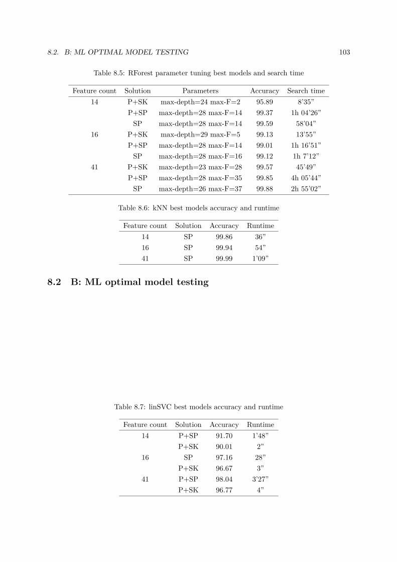
8.2. B: ML OPTIMAL MODEL TESTING 103
Table 8.5: RForest parameter tuning best models and search time
Feature count Solution Parameters Accuracy Search time14 P+SK max-depth=24 max-F=2 95.89 8’35”
P+SP max-depth=28 max-F=14 99.37 1h 04’26”SP max-depth=28 max-F=14 99.59 58’04”
16 P+SK max-depth=29 max-F=5 99.13 13’55”P+SP max-depth=28 max-F=14 99.01 1h 16’51”
SP max-depth=28 max-F=16 99.12 1h 7’12”41 P+SK max-depth=23 max-F=28 99.57 45’49”
P+SP max-depth=28 max-F=35 99.85 4h 05’44”SP max-depth=26 max-F=37 99.88 2h 55’02”
Table 8.6: kNN best models accuracy and runtime
Feature count Solution Accuracy Runtime14 SP 99.86 36”16 SP 99.94 54”41 SP 99.99 1’09”
8.2 B: ML optimal model testing
Table 8.7: linSVC best models accuracy and runtime
Feature count Solution Accuracy Runtime14 P+SP 91.70 1’48”
P+SK 90.01 2”16 SP 97.16 28”
P+SK 96.67 3”41 P+SP 98.04 3’27”
P+SK 96.77 4”
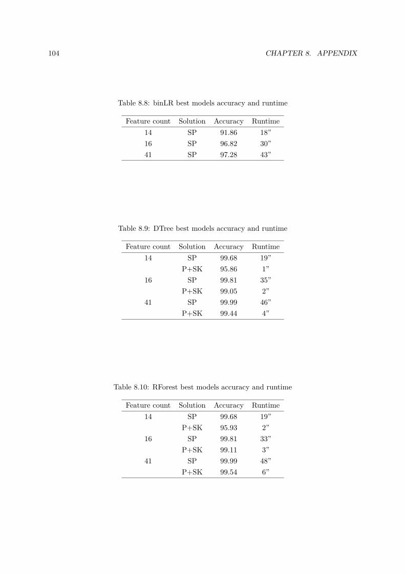
104 CHAPTER 8. APPENDIX
Table 8.8: binLR best models accuracy and runtime
Feature count Solution Accuracy Runtime14 SP 91.86 18”16 SP 96.82 30”41 SP 97.28 43”
Table 8.9: DTree best models accuracy and runtime
Feature count Solution Accuracy Runtime14 SP 99.68 19”
P+SK 95.86 1”16 SP 99.81 35”
P+SK 99.05 2”41 SP 99.99 46”
P+SK 99.44 4”
Table 8.10: RForest best models accuracy and runtime
Feature count Solution Accuracy Runtime14 SP 99.68 19”
P+SK 95.93 2”16 SP 99.81 33”
P+SK 99.11 3”41 SP 99.99 48”
P+SK 99.54 6”