Embed Size (px)
Citation preview

VOL. VOL NO. ISSUE NETWORK STRUCTURE AND INFORMATION AGGREGATION 47
Network Structure and the Aggregation of Information: Theory andEvidence from Indonesia
Vivi Alatas, Abhijit Banerjee, Arun G. Chandrasekhar, Rema Hanna, andBenjamin A. Olken
Online Appendix
Network definitions
In this section, we provide basic definitions and interpretations for the differentnetwork characteristics that we consider. See Jackson (2008) for details. At thehousehold level, we study:
• Degree: the number of links that a household has. This is a measure of howwell connected a node is in the graph.
• Clustering coefficient: the fraction of a household’s neighbors that are them-selves neighbors. This is a measure of how interwoven a household’s neigh-borhood is.
• Eigenvector centrality: recursively defined notion of importance. A house-hold’s importance is defined to be proportional to the sum of its neighbors’importances. It corresponds to the ith entry of the eigenvector correspond-ing to the maximal eigenvalue of the adjacency matrix. This is a measureof how important a node is, in the sense of information flow. We take theeigenvector normalized with ‖·‖2 = 1.
• Reachability and distance: we say two households i and j are reachable ifthere exists a path through the network that connects them. The distanceis the length of the shortest such path.
At the hamlet level, we consider:
• Average degree: the mean number of links that a household has in thehamlet. A network with higher average degree has more edges on which totransmit information.
• Average clustering: the mean clustering coefficient of households in thehamlet. This measures how interwoven the network is.
• Average path length: the mean length of the shortest path between any twohouseholds in the hamlet which are connected. Shorter average path lengthmeans information has to travel less (on average) to get from household ito household j.

48 THE AMERICAN ECONOMIC REVIEW MONTH YEAR
• First eigenvalue: the largest eigenvalue of the adjacency matrix. This is ameasure of how diffusive the network is. A higher first eigenvalue tends tomean that information is generally transmitted more.
• Fraction of nodes in the giant component: the share of nodes in the graphthat are in the largest connected component. Typically, realistic graphshave a “giant” component with almost all nodes in it. Thus, the measureshould be approaching one. For a network that is sampled, this numbercan be significantly lower. In particular, networks which were tenuouslyor sparsely connected to begin with, may “shatter” under sampling andtherefore the giant component may no longer be giant after sampling. Inturn, it becomes a useful measure of how interwoven the underlying networkis.
• Link density: the average share of connections (out of potential connections)that a household has. This measure looks at the rate of edge formation ina graph.

VOL. VOL NO. ISSUE NETWORK STRUCTURE AND INFORMATION AGGREGATION 49
Kalman Filter, Estimation and Simulation
This section develops the formal algorithm for the model and discusses estima-tion.
B1. Model
Setup
Without loss of generality, fix node j about whose wealth the remainder of thenodes are learning. Wealth follows an AR(1) process given by
wj,t = c+ ρwj,t−1 + εj,t.
Individuals i ∈ V\{j} want to guess wj,t when surveyed at period t, given an
information set F ji,t−1 that is informed from social learning.The model will have a transmission error in every step when an individual
speaks to another individual. For instance, if l communicates with i in period r,this communication can be disturbed by some ul 7→ir . We will assume that everyul 7→ir is independently and identically distributed, N
(0, σ2
u
)with common mean
and variance.Individuals communicate with each others as follows. At period t we look at
what node i receives from others and consider her updating problem:
• Signals from the source j: Every period, the source j generates a signalabout her t− 1 wealth that she transmits to each of her neighbors, i ∈ Nj .
Sj 7→it−1 = wj,t−1 + uj 7→it−1 .
• Signals from arbitrary node l to i: Every period, a node l noisily transmitsthe most recent piece of gossip she has heard to each of her neighbors,independently.
– Let k∗ := k∗ (l, j) be the neighbor of l that is closest to j.36 The signalthat l received from k∗ the previous period is what will then be passedon.
– Passing only occurs if l is sufficiently sure enough about the qualityof this information. This is mapped to some threshold τ such that ifd (k∗ (l, j) , j) ≤ τ , then l passes information to each of her neighbors.If d (k∗ (l, j) , j) > τ , then no information is passed.
– When l passes information, it is
Sl 7→it−d(l,j) = Sk∗ 7→lt−1−d(k∗,j) + ul 7→it−d(l,j).
36For presentation purposes we assume this is unique. If it is not unique, and there are two suchclosest signals, then we assume that l passes the average.
50 THE AMERICAN ECONOMIC REVIEW MONTH YEAR
The above protocol defines a signal generation process. Thus, in every period t,a generic node i in the graph has received a vector of signals
si,t :=(si,t1 , ..., s
i,tt−d(i,j)
).
This vector of signals encodes the information that i has about each wj,1, ..., wj,t−d(i,j).
Note that the signal vector si,t is double-indexed since it can have time-varyingelements.
• The signal vector can treated as a collection of independent draws (condi-tional on the wealth sequence) with
si,tr ∼ N(wj,r, σ
2r,t,i
)where i’s tth period signal about wj,r can only come from neighbors thatare close enough to j,
si,tr =∑l∈Ni
ωl,r,t,i · Sl 7→ir ,
and ωl,r,t,i =1{t−r≥d(l,j)+1}/[σ2
u,d(l,j)]∑k∈Ni
1{t−r≥d(k,j)+1}/[σ2ud(k,j)]
is the weight that i puts on l in
period t about l’s estimate of wj,r.
This is because only neighbors of i that are within t − r − 1 steps of jcan reveal an estimate of wj,r to i by period t. Every time the signal istransferred across individuals, it is disturbed by a shock with variance σ2
u,leading to a variance of σ2
u ·d (l, j) for a signal that has traveled d (l, j) steps.
In this case, we can compute i’s period t variance about wj,r as
σ2r,t,i =
∑l∈Ni
ω2l,r,t,i · σ2
ud (l, j) .
• Given si,t, node i applies the Kalman filter to obtain the posterior meanand variance over wj,t.
Kalman Filter
The Kalman filter is as follows. In what follows, we reserve r to index time(and describe the process only for nodes that are speaking). At period t a nodei makes the following computation. She treats the system as the tth period of alinear Gauss-Markov dynamical system with
• state equation is given by
wj,r = c+ ρwj,r−1 + εj,r, r = 1, ..., t+ 1.

VOL. VOL NO. ISSUE NETWORK STRUCTURE AND INFORMATION AGGREGATION 51
• measurement equation given by
si,tr = wj,r + vi,tr ,
where vi,tr ∼ N(
0, σ2r,t,i
).
Then the computation of the Kalman filter is entirely standard given the vectorsi,t of measurements and knowledge of parameters c, ρ, σ2
ε , σ2u and d (k, j) ∀k ∈ Ni.
The crucial equations are how to do a time update given prior information andhow to incorporate the new measurements to correct the system:
• Time update equations:
w−r = ρwr−1 + c
P−r = ρ2Pr−1 + σ2ε .
• Measurement update equations:
Kr =P−r
P−r + σ2r,t,i
.
wr = w−r +Kr
(si,tr − w−r
).
Pr = (1−Kr)P−r .
The initialization is at the mean of the invariant distribution w0 = c1−ρ and the
variance P0 = σ2ε
1−ρ2 .
B2. Estimation
Before conducting our simulated method of moments, we first estimate somepreliminary parameters.
1) Auto-correlation parameter (ρ): We use data from Indonesia Family LifeSurvey. We construct a panel data for 1993, 1997, 2000, and 2007. Thesample used contains only those households that were surveyed in all theyears. We use real total expenditures as our variable of interest.37 As therewas a financial crisis in 1997-1998, we omit the 1997-2000 period from theestimation. Given that the gap between the years is long and variable, weuse the mean gap to compute an approximate yearly ρ. The mean gap is 5.5years so we obtain ρ using (ρ)k = ρPanel, for k = 5.5, and its distribution isderived using the delta method. We estimate ρ = 0.86 and because of thesize of the panel, the parameter is tightly estimated (a t-statistic of 12.33);thus, we view it as super-consistent relative to the structural parameters inour model.
37Expenditures were converted in real terms using the CPI published by the Central Bank.

52 THE AMERICAN ECONOMIC REVIEW MONTH YEAR
2) Variance of the shock term (σ2ε ): We obtain this variable using the station-
ary variance of the consumption process σ2w = σ2
ε(1−ρ2)
. Again, given the size
of the data set this can be viewed as super-consistent.
B3. Simulated Method of Moments
Equipped with a collection of over 600 graphs, ρ, and σ2ε , we estimate our model
via simulated method of moments. The two parameters we are interested in are
(α, τ) where α := σ2uσ2ε
and τ is the maximal distance away from the source for an
individual to be confident enough to pass information to her neighbors.Our approach is a grid-based simulated method of moments which allows us to
conduct inference on a large simulation quite easily (Banerjee et al., 2013). Welet Θ be the parameter space and Ξ be a grid on Θ, which we describe below.We put ψ(·) as the moment function and let zr = (yr, xr) denote the empiricaldata for network r with a vector of wealth ranking decisions for each surveyedindividual, yr, as well as data, xr, which includes expenditure data and the graphGr.
Definememp,r := ψ(zr) as the empirical moment for hamlet r andmsim,r(s, θ) :=ψ(zsr(θ)) = ψ(ysr(θ), xr) as the sth simulated moment for hamlet r at parametervalue θ. Finally, put B as the number of bootstraps and S as the number ofsimulations used to construct the simulated moment. This nests the case withB = 1 in which we just find the minimizer of the objective function.
1) Pick lattice Ξ ⊂ Θ. For ξ ∈ Ξ on the grid:
a) For each network r ∈ [R], compute
d(r, ξ) :=1
S
∑s∈[S]
msim,r(s, θ)−memp,r.
b) For each b ∈ [B], compute
D(b, ξ) :=1
R
∑r∈[R]
ωbr · d(r, ξ)
where ωbr = ebr/er, with ebr iid exp(1) random variables and er =1R
∑ebr if we are conducting bootstrap, and ωbr = 1 if we are just
finding the minimizer.
c) Find ξ?b = argmin Q?b(ξ), with Q?b (ξ) = D(b, ξ)′D(b, ξ).38
2) Obtain {ξ?b}b∈B.
38Because we are just identified we do not need to weight the moments.
VOL. VOL NO. ISSUE NETWORK STRUCTURE AND INFORMATION AGGREGATION 53
3) For conservative inference on θj , the jth component, consider the 1 − α/2and α/2 quantiles of the ξ?bj marginal empirical distribution.
In all simulations we use B = 10000, S = 50. We set Ξ = [0.1 : 0.033 : 0.85] ×{1, ..., 7}.
B4. Simulations for Regressions
To generate our synthetic data we fix our parameters (α, τ) and generate 50draws. We then compute
ErrorSIMijkr =
∑s
Errorsijkr/50.
This allows us to aggregate the errors to any level we need. For instance by
integrating over all the triples in our sample, we can compute ErrorSIMr , the
simulated error rate for hamlet r. We then conduct our regression analysis withthese simulated outcomes.

54 THE AMERICAN ECONOMIC REVIEW MONTH YEAR
Details on Poverty Targeting Procedures
This appendix briefly describes the poverty targeting procedures used to al-locate the transfer program to households. Additional details can be found inAlatas et al. (2012).
• PMT Treatment: the government created formulas that mapped 49 eas-ily observable household characteristics into a single index using regressiontechniques.39 Government enumerators collected these indicators from allhouseholds in the PMT hamlets by conducting a door-to-door survey. Thesedata were then used to calculate a computer-generated predicted consump-tion score for each household using a district-specific PMT formula. A listof beneficiaries was generated by selecting the pre-determined number ofhouseholds with the lowest scores in each hamlet, based on quotes deter-mined by a geographic targeting procedure.
• Community Treatment: To start, a local facilitator visited each hamlet topublicize the program and invite individuals to a community meeting.40 Atthe meeting, the facilitator first explained the program. Next, he or shedisplayed the list of all households in the hamlet (which came from thebaseline survey). The facilitator then spent about 15 minutes having thecommunity brainstorm a list of characteristics that differentiate the poorfrom the wealthy households in their community. The facilitator then pro-ceeded with the ranking exercise using a set of randomly-ordered index cardsthat displayed the names of each household in the neighborhood. He or shehung a string from wall to wall, with one end labeled as “most well-off”(paling mampu) and the other side labeled as “poorest” (paling miskin).Then, he or she started by holding up the first two name cards from therandomly-ordered stack and asking the community, “Which of these twohouseholds is better off?” Based on the community’s response, he or she at-tached the cards along the string, with the poorer household placed closerto the “poorest” end. Next, the facilitator displayed the third card andasked how this household ranked relative to the first two households. Theactivity continued with each card being positioned relative to the already-ranked households one-by-one until complete. Before the final ranking wasrecorded, the facilitator read the ranking aloud so adjustments could bemade if necessary. After all meetings were complete, the facilitators were
39The chosen indicators encompassed the household’s home attributes (wall type, roof type, etc),assets (TV, motorbike, etc), household composition, and household head’s education and occupation.The formulas were derived using pre-existing survey data: specifically, the government estimated therelationship between the variables of interest and household per capita consumption. While the sameindicators were considered across regions, the government estimated district-specific formulas due to theperceived high variance in the best predictors of poverty across regions
40On average, 45 percent of households attended the meeting. Note, however, that we only invitedthe full community in half of the community treatment hamlets. In the other half (randomly selected),only local elites were invited, so that we can see whether elites are more likely to capture the communityprocess when they have control over the process.

VOL. VOL NO. ISSUE NETWORK STRUCTURE AND INFORMATION AGGREGATION 55
provided with “beneficiary quotas” for each hamlet based on the geographictargeting procedure. Households ranked below the quota were deemed eli-gible.
• Hybrid Treatment: This method combines the community ranking proce-dure with a subsequent PMT verification. The ranking exercise, describedabove, was implemented first. However, there was one key difference: atthe start of these meetings, the facilitator announced that the lowest-rankedhouseholds would be independently checked by the government enumera-tors before the beneficiary list was finalized. After the community meet-ings were complete, the government enumerators indeed visited the lowest-ranked households to collect the data needed to calculate their PMT score.The number of households to be visited was computed by multiplying the“beneficiary quotas” by 150 percent. Households were ranked by their PMTscore, and those below the village quota became beneficiaries of the program.Thus, it was possible that some households could become beneficiaries evenif they were ranked as slightly wealthier than the beneficiary quota cutoffline on the community list. Conversely, some relatively poor-ranked house-holds on the community list might become ineligible.

56 THE AMERICAN ECONOMIC REVIEW MONTH YEAR
Tables without Don’t Knows
Table D1—: The Correlation between Household Network Characteristics andthe Error Rate in Ranking Income Status of Household, Conditional on OfferingAssessments
(1) (2) (3) (4)
Degree -0.00285 -0.00184(0.000712) (0.00116)
Clustering -0.0119 -0.00870(0.00892) (0.00985)
Eigenvector Centrality -0.0865 -0.0421(0.0233) (0.0382)
R-squared 0.665 0.663 0.665 0.665
Degree -0.00389 -0.00275(0.000712) (0.00122)
Clustering -0.00282 0.000356(0.00998) (0.0108)
Eigenvector Centrality -0.105 -0.0461(0.0247) (0.0410)
R-squared 0.671 0.669 0.671 0.672
Hamlet Fixed Effect Yes Yes Yes Yes
Outcome variable: Error rate conditional on reportingPanel A: Consumption Metric
Panel B: Self-Assessment Metric
Notes: This table provides estimates of the correlation between a household’s network characteristics and itsability to accurately rank the poverty status of other members of the hamlet. The sample comprises 5,621households. The mean of the dependent variable in Panel A (a household’s error rate in ranking others in thehamlet based on consumption) is 0.52, while the mean of the dependent variable in Panel B (a household'serror rate in ranking others in the hamlet based on a household's own self-assessment of poverty status) is0.46. "Don't know" answers are dropped. Standard errors are clustered by hamlet and are listed inparentheses.

VOL. VOL NO. ISSUE NETWORK STRUCTURE AND INFORMATION AGGREGATION 57
Table D2—: The Correlation between Household Network Characteristics and theError Rate in Ranking Income Status of Household, Controlling for HouseholdCharacteristics, Conditional on Offering Assessments
(1) (2) (3) (4)
Degree -0.00218 -0.00129(0.000696) (0.00112)
Clustering -0.0117 -0.00861(0.00878) (0.00973)
Eigenvector Centrality -0.0697 -0.0373(0.0231) (0.0374)
R-squared 0.668 0.667 0.668 0.668
Degree -0.00305 -0.00207(0.000696) (0.00118)
Clustering -0.00267 0.000220(0.00970) (0.0106)
Eigenvector Centrality -0.0834 -0.0395(0.0243) (0.0400)
R-squared 0.676 0.675 0.676 0.676
Hamlet Fixed Effect Yes Yes Yes Yes
Outcome variable: Error rate conditional on reportingPanel A: Consumption Metric
Panel B: Self-Assessment Metric
Notes: This table provides estimates of the correlation between a household’s network characteristics and itsability to accurately rank the poverty status of other members of the hamlet, controlling for the household'scharacteristics as in Table 3. The sample comprises 5,621 households for panel. The mean of the dependentvariable in Panel A (a household’s error rate in ranking others in the hamlet based on consumption) is 0.52, whilethe mean of the dependent variable in Panel B (a household's error rate in ranking others in the hamlet based on ahousehold's own self-assessment of poverty status) is 0.46. "Don't know" answers are dropped. Standard errorsare clustered by hamlet and are listed in parentheses.

58 THE AMERICAN ECONOMIC REVIEW MONTH YEAR
Table D3—: The Correlation Between Inaccuracy in Ranking a Pair of Householdsin a Hamlet and the Average Inverse Distance to Rankees, Conditional on OfferingAssessments
(1) (2) (3) (4)
Average Inverse Distance -0.00645 -0.0178 -0.00886 -0.0215(0.00662) (0.00660) (0.00491) (0.0132)
Average Degree 0.00139 0.00571 0.00628(0.00140) (0.00307) (0.00320)
Average Clustering Coefficient 0.0252 0.0618 0.0693(0.0228) (0.0266) (0.0280)
Average Eigenvector Centrality -0.0480 -0.177 -0.153(0.0547) (0.1000) (0.106)
R-squared 0.000 0.008 0.082 0.139
Average Inverse Distance -0.00802 -0.0143 -0.00458 0.00230(0.00689) (0.00694) (0.00507) (0.0131)
Average Degree 0.000997 0.00175 0.00118(0.00146) (0.00297) (0.00312)
Average Clustering Coefficient -0.0216 0.0228 0.0242(0.0237) (0.0289) (0.0300)
Average Eigenvector Centrality 0.0298 0.0304 0.0346(0.0549) (0.0993) (0.104)
R-squared 0.000 0.002 0.092 0.168
Demographic Controls No Yes Yes YesHamlet Fixed Effect No No Yes YesRanker Fixed Effect No No No Yes
Outcome variable: Error rate conditional on reportingPanel A: Consumption Metric
Panel B: Self-Assessment Metric
Notes: This table provides an estimate of the correlation between the accuracy in ranking a pair of households in a hamlet and the characteristics of the households that are being ranked. In Panel A, the dependent variable is a dummy variable for whether household i ranks household j versus household k incorrectly based on using consumption as the metric of truth (the sample mean is 0.52). In Panel B, the self-assessment variable is the metric of truth (the sample mean is 0.46). "Don't know" answers are dropped. The sample is comprised of 81,162 ranked pairs in Panel A and 80,380 in Panel B. Standard errors are clustered by hamlet and are listed in parentheses.

VOL. VOL NO. ISSUE NETWORK STRUCTURE AND INFORMATION AGGREGATION 59
Extended Micro Tables Using Simulations
Table E1—: The Correlation between Household Network Characteristics andthe Error Rate in Ranking Income Status of Households, Including Simulations
(1) (2) (3) (4) (5) (6) (7) (8)
Degree -0.00285 -0.00189 -0.00305 -0.00153(0.000710) (0.00115) (0.000672) (0.00115)
Clustering -0.0128 -0.00970 0.000603 0.00339(0.00889) (0.00980) (0.0111) (0.0122)
Eigenvector Centrality -0.0859 -0.0399 -0.0950 -0.0622(0.0232) (0.0379) (0.0258) (0.0415)
R-squared 0.667 0.666 0.667 0.667 0.719 0.717 0.719 0.719
Degree -0.00388 -0.00282 -0.00305 -0.00153(0.000715) (0.00121) (0.000672) (0.00115)
Clustering -0.00415 -0.00124 0.000603 0.00339(0.0100) (0.0109) (0.0111) (0.0122)
Eigenvector Centrality -0.104 -0.0427 -0.0950 -0.0622(0.0248) (0.0408) (0.0258) (0.0415)
R-squared 0.674 0.672 0.674 0.674 0.719 0.717 0.719 0.719
Degree -0.00836 -0.00465 -0.0166 -0.00946(0.000576) (0.000782) (0.00113) (0.00153)
Clustering -0.0778 -0.0704 -0.157 -0.143(0.00740) (0.00714) (0.0146) (0.0142)
Eigenvector Centrality -0.309 -0.175 -0.612 -0.339(0.0187) (0.0264) (0.0368) (0.0518)
R-squared 0.896 0.887 0.905 0.913 0.902 0.893 0.912 0.921
Hamlet Fixed Effect Yes Yes Yes Yes Yes Yes Yes YesNotes: This table provides estimates of the correlation between a household’s network characteristics and its ability to accurately rank the poverty status of other members ofthe hamlet. The sample comprises 5,649 households. The mean of the dependent variable in Panel A (a household’s error rate in ranking others in the hamlet based onconsumption) is 0.52, while the mean of the dependent variable in Panel B (a household's error rate in ranking others in the hamlet based on a household's own self-assessmentof poverty status) is 0.46. Details of the simulation procedure for Panel C are contained in Appendix B. Standard errors are clustered by hamlet and are listed in parentheses.
Panel C: Simulations
Outcome variable: Error rate Outcome variable: Share of don't knowsPanel A: Consumption Metric
Panel B: Self-Assessment Metric

60 THE AMERICAN ECONOMIC REVIEW MONTH YEAR
Table E2—: The Correlation between Household Network Characteristics and theError Rate in Ranking Income Status of Households, Controlling for HouseholdCharacteristics, Including Simulations
(1) (2) (3) (4) (5) (6) (7) (8)
Degree -0.00217 -0.00133 -0.00235 -0.000900(0.000695) (0.00111) (0.000663) (0.00113)
Clustering -0.0125 -0.00964 -0.000466 0.00296(0.00876) (0.00969) (0.0109) (0.0119)
Eigenvector Centrality -0.0689 -0.0351 -0.0783 -0.0596(0.0230) (0.0370) (0.0254) (0.0406)
R-squared 0.671 0.670 0.671 0.671 0.723 0.722 0.723 0.723
Degree -0.00302 -0.00212 -0.00235 -0.000900(0.000699) (0.00118) (0.000663) (0.00113)
Clustering -0.00398 -0.00136 -0.000466 0.00296(0.00976) (0.0107) (0.0109) (0.0119)
Eigenvector Centrality -0.0819 -0.0361 -0.0783 -0.0596(0.0243) (0.0398) (0.0254) (0.0406)
R-squared 0.679 0.678 0.679 0.679 0.723 0.722 0.723 0.723
Degree -0.00833 -0.00461 -0.0166 -0.00941(0.000576) (0.000779) (0.00113) (0.00152)
Clustering -0.0780 -0.0701 -0.157 -0.142(0.00734) (0.00711) (0.0145) (0.0141)
Eigenvector Centrality -0.309 -0.176 -0.611 -0.340(0.0187) (0.0264) (0.0368) (0.0517)
R-squared 0.896 0.888 0.906 0.914 0.903 0.894 0.913 0.921
Hamlet Fixed Effect Yes Yes Yes Yes Yes Yes Yes YesNotes: This table provides estimates of the correlation between a household’s network characteristics and its ability to accurately rank the poverty status of other members ofthe hamlet, controlling for the household's characteristics as in Table 3. The sample comprises 5,646 households for panel. The mean of the dependent variable in Panel A (ahousehold’s error rate in ranking others in the hamlet based on consumption) is 0.52, while the mean of the dependent variable in Panel B (a household's error rate in rankingothers in the hamlet based on a household's own self-assessment of poverty status) is 0.46. Details of the simulation procedure for Panel C are contained in Appendix B.Standard errors are clustered by hamlet and are listed in parentheses.
Panel C: Simulations
Outcome variable: Error rate Outcome variable: Share of don't knowsPanel A: Consumption Metric
Panel B: Self-Assessment Metric

VOL. VOL NO. ISSUE NETWORK STRUCTURE AND INFORMATION AGGREGATION 61
Table E3—: The Correlation between Inaccuracy in Ranking a Pair of Householdsin a Hamlet and the Average Distance to Rankees, Including Simulations
(1) (2) (3) (4) (5) (6) (7) (8)
Average Inverse Distance -0.0574 -0.0380 -0.0222 -0.0158 -0.0737 -0.0414 -0.0280 -0.00756(0.00846) (0.00834) (0.00571) (0.0127) (0.00950) (0.00992) (0.00707) (0.0132)
Average Degree -0.00501 0.00243 0.00258 -0.00961 -0.00257 -0.00270(0.00176) (0.00318) (0.00323) (0.00212) (0.00309) (0.00309)
Average Clustering Coefficient 0.00181 0.0326 0.0338 -0.0298 -0.0132 -0.0144(0.0256) (0.0275) (0.0279) (0.0307) (0.0288) (0.0286)
Average Eigenvector Centrality 0.0464 -0.0856 -0.111 0.129 0.0881 0.0232(0.0674) (0.0923) (0.0954) (0.0825) (0.0985) (0.105)
R-squared 0.007 0.011 0.136 0.202 0.019 0.061 0.330 0.443
Average Inverse Distance -0.0664 -0.0390 -0.0219 -0.00629 -0.0737 -0.0414 -0.0280 -0.00756(0.00952) (0.00918) (0.00601) (0.0137) (0.00950) (0.00992) (0.00707) (0.0132)
Average Degree -0.00614 9.26e-05 -0.000375 -0.00961 -0.00257 -0.00270(0.00194) (0.00340) (0.00349) (0.00212) (0.00309) (0.00309)
Average Clustering Coefficient -0.0354 0.00674 0.00838 -0.0298 -0.0132 -0.0144(0.0275) (0.0304) (0.0304) (0.0307) (0.0288) (0.0286)
Average Eigenvector Centrality 0.111 0.0420 0.00617 0.129 0.0881 0.0232(0.0758) (0.105) (0.108) (0.0825) (0.0985) (0.105)
R-squared 0.009 0.019 0.166 0.247 0.019 0.061 0.330 0.443
Average Inverse Distance -0.260 -0.225 -0.202 -0.240 -0.521 -0.450 -0.404 -0.479(0.00232) (0.00287) (0.00503) (0.00836) (0.00373) (0.00488) (0.00933) (0.0155)
Average Degree -0.00575 -0.00423 -0.00277 -0.0114 -0.00982 -0.00714(0.000716) (0.00137) (0.00145) (0.00108) (0.00240) (0.00255)
Average Clustering Coefficient -0.0916 -0.128 -0.123 -0.187 -0.256 -0.248(0.0116) (0.0136) (0.0147) (0.0197) (0.0243) (0.0266)
Average Eigenvector Centrality -0.0841 -0.218 -0.151 -0.150 -0.386 -0.248(0.0257) (0.0439) (0.0451) (0.0389) (0.0791) (0.0802)
R-squared 0.504 0.524 0.593 0.621 0.745 0.763 0.827 0.857
Demographic Controls No Yes Yes Yes No Yes Yes YesHamlet Fixed Effects No No Yes Yes No No Yes YesRanker Fixed Effects No No No Yes No No No Yes
Notes: This table provides an estimate of the correlation between the accuracy in ranking a pair of households in a hamlet and the characteristics of the households that arebeing ranked. In Panel A, the dependent variable is a dummy variable for whether household i ranks household j versus household k incorrectly based on using consumption asthe metric of truth (the sample mean is 0.52). In Panel B, the self-assessment variable is the metric of truth (the sample mean is 0.46). The sample is comprised of 104,417ranked pairs in Panel A and 103,435 in Panel B. Details of the simulation procedure for Panel C are contained in Appendix B. Standard errors are clustered by hamlet and arelisted in parentheses.
Panel C: Simulations
Outcome variable: Error rate Outcome variable: Share of don't knowsPanel A: Consumption Metric
Panel B: Self-Assessment Metric

62 THE AMERICAN ECONOMIC REVIEW MONTH YEAR
Tables without Demographic Covariates
Table F1—: Without Controls: Numerical Predictions on Correlation betweenHamlet Network Characteristics and Hamlet Level Error Rates
(1) (2) (3) (4) (5) (6) (7)
Average Degree -0.0283 0.0802(0.00233) (0.00792)
Average Clustering -0.349 0.430(0.0362) (0.0754)
Number of Households 0.00108 0.000610(0.000263) (0.000283)
First eigenvalue λ1(A) -0.0279 -0.0546(0.00215) (0.00469)
Fraction of Nodes in Giant Component -0.382 -0.749(0.0240) (0.0514)
Link Density -0.543 -0.545(0.0677) (0.0922)
R-squared 0.182 0.126 0.028 0.245 0.281 0.107 0.483Notes: Same as Table 7, without demographic controls. It reports the relationship between hamlet network characteristics and the error rate in ranking others in the hamlet. Columns 1-6 show univariate regressions, while column 7 reports the results from a multvariate regression. The sample comprises 631 hamlets. Results for error rates using simulated data, as described in Appendix B. Robust standard errors in parentheses.

VOL. VOL NO. ISSUE NETWORK STRUCTURE AND INFORMATION AGGREGATION 63
Table F2—: Without Controls: Numerical Predictions on Correlation betweenHamlet Network Characteristics and Hamlet Level Error Rates
(1) (2) (3) (4) (5) (6) (7)
Average Degree -0.0200 0.0356(0.00274) (0.0112)
Average Clustering -0.361 -0.359(0.0406) (0.0953)
Number of Households 0.000892 0.000305(0.000301) (0.000391)
First eigenvalue λ1(A) -0.0168 -0.0211(0.00217) (0.00578)
Fraction of Nodes in Giant Component -0.264 -0.205(0.0300) (0.0699)
Link Density -0.349 0.108(0.0780) (0.138)
R-squared 0.076 0.114 0.016 0.075 0.113 0.037 0.153
Average Degree -0.0276 0.0294(0.00294) (0.0124)
Average Clustering -0.495 -0.476(0.0431) (0.106)
Number of Households 0.00135 0.000266(0.000337) (0.000418)
First eigenvalue λ1(A) -0.0206 -0.0165(0.00251) (0.00660)
Fraction of Nodes in Giant Component -0.355 -0.219(0.0319) (0.0779)
Link Density -0.524 0.163(0.0816) (0.148)
R-squared 0.115 0.170 0.029 0.090 0.161 0.066 0.198
Panel A: Consumption Metric
Panel B: Self-Assessment Metric
Notes: Same as Table 9, without demographic controls. It reports the relationship between hamlet network characteristics and the error rate in ranking others in the hamlet. Columns 1-6 show univariate regressions, while column 7 reports the results from a multvariate regression. The sample comprises 631 hamlets. Panel A presents results for error rates using the consumption metric. Panel B presents results for error rates using the self-assessment metric. Robust standard errors in parentheses.
64 THE AMERICAN ECONOMIC REVIEW MONTH YEAR
Alternative Parameters
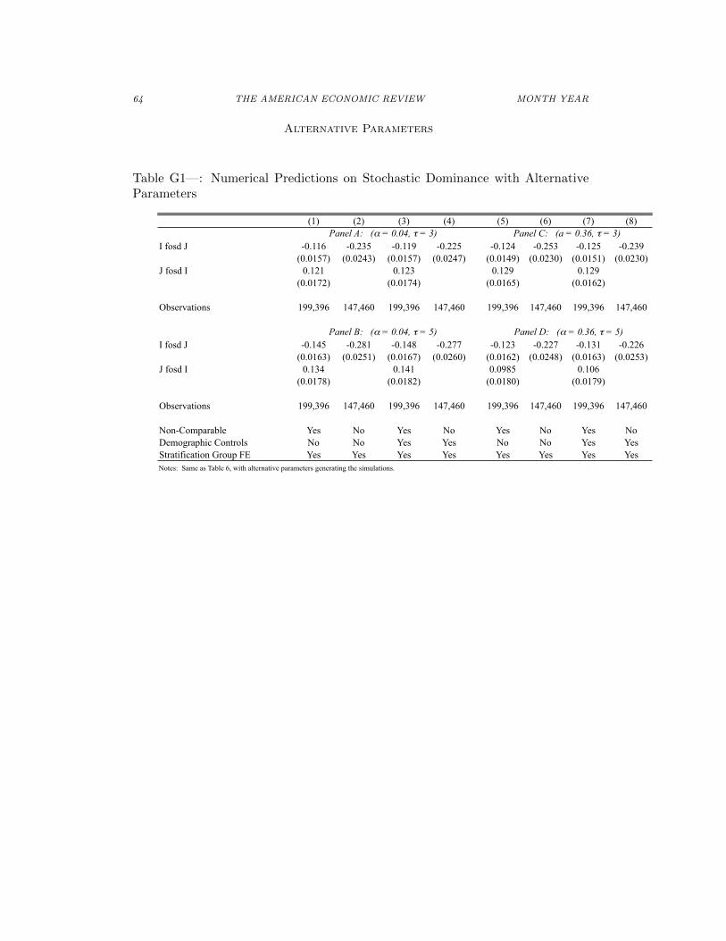
Table G1—: Numerical Predictions on Stochastic Dominance with AlternativeParameters
(1) (2) (3) (4) (5) (6) (7) (8)
I fosd J -0.116 -0.235 -0.119 -0.225 -0.124 -0.253 -0.125 -0.239(0.0157) (0.0243) (0.0157) (0.0247) (0.0149) (0.0230) (0.0151) (0.0230)
J fosd I 0.121 0.123 0.129 0.129(0.0172) (0.0174) (0.0165) (0.0162)
Observations 199,396 147,460 199,396 147,460 199,396 147,460 199,396 147,460
I fosd J -0.145 -0.281 -0.148 -0.277 -0.123 -0.227 -0.131 -0.226(0.0163) (0.0251) (0.0167) (0.0260) (0.0162) (0.0248) (0.0163) (0.0253)
J fosd I 0.134 0.141 0.0985 0.106(0.0178) (0.0182) (0.0180) (0.0179)
Observations 199,396 147,460 199,396 147,460 199,396 147,460 199,396 147,460
Non-Comparable Yes No Yes No Yes No Yes NoDemographic Controls No No Yes Yes No No Yes YesStratification Group FE Yes Yes Yes Yes Yes Yes Yes YesNotes: Same as Table 6, with alternative parameters generating the simulations.
Panel B: (α = 0.04, τ = 5)
Panel A: (α = 0.04, τ = 3) Panel C: (a = 0.36, τ = 3)
Panel D: (α = 0.36, τ = 5)

VOL. VOL NO. ISSUE NETWORK STRUCTURE AND INFORMATION AGGREGATION 65
Tab
leG
2—:
Nu
mer
ical
Pre
dic
tion
son
Sto
chas
tic
Dom
inan
cew
ith
Alt
ern
ativ
eP
aram
eter
s
(1)
(2)
(3)
(4)
(5)
(6)
(7)
(8)
(9)
(10)
(11)
(12)
(13)
(14)
Aver
age
Deg
ree
-0.0
304
0.08
38-0
.031
20.
0782
(0.0
0268
)(0
.008
13)
(0.0
0272
)(0
.008
14)
Aver
age
Clu
ster
ing
-0.3
620.
325
-0.3
740.
319
(0.0
433)
(0.0
754)
(0.0
433)
(0.0
761)
Num
ber o
f Hou
seho
lds
0.00
0942
0.00
0521
0.00
0963
0.00
0510
(0.0
0025
1)(0
.000
272)
(0.0
0025
1)(0
.000
278)
Firs
t eig
enva
lue λ 1
(A)
-0.0
294
-0.0
581
-0.0
297
-0.0
558
(0.0
0236
)(0
.005
06)
(0.0
0233
)(0
.004
99)
Frac
tion
of N
odes
in G
iant
Com
pone
nt-0
.423
-0.6
88-0
.429
-0.6
80(0
.027
3)(0
.052
9)(0
.027
1)(0
.053
1)Li
nk D
ensi
ty-0
.535
-0.6
34-0
.540
-0.5
73(0
.073
3)(0
.089
9)(0
.076
0)(0
.092
3)R
-squ
ared
0.24
20.
181
0.10
50.
308
0.32
20.
173
0.51
00.
248
0.18
40.
103
0.31
10.
327
0.17
10.
504
Aver
age
Deg
ree
-0.0
295
0.07
52-0
.029
00.
0780
(0.0
0278
)(0
.007
82)
(0.0
0278
)(0
.007
86)
Aver
age
Clu
ster
ing
-0.3
590.
374
-0.3
550.
372
(0.0
431)
(0.0
722)
(0.0
434)
(0.0
730)
Num
ber o
f Hou
seho
lds
0.00
0879
0.00
0253
0.00
0897
0.00
0298
(0.0
0025
2)(0
.000
300)
(0.0
0024
9)(0
.000
282)
Firs
t eig
enva
lue λ 1
(A)
-0.0
281
-0.0
508
-0.0
278
-0.0
519
(0.0
0241
)(0
.004
62)
(0.0
0238
)(0
.004
55)
Frac
tion
of N
odes
in G
iant
Com
pone
nt-0
.446
-0.8
11-0
.442
-0.8
10(0
.026
9)(0
.049
0)(0
.026
9)(0
.049
3)Li
nk D
ensi
ty-0
.476
-0.4
24-0
.475
-0.4
53(0
.073
4)(0
.086
2)(0
.075
7)(0
.087
1)R
-squ
ared
0.23
20.
176
0.09
40.
292
0.35
60.
150
0.54
60.
224
0.17
10.
092
0.28
50.
350
0.14
60.
543
Not
es: S
ame
as T
able
7, w
ith a
ltern
ativ
e pa
ram
eter
s gen
erat
ing
the
sim
ulat
ions
.
Pane
l C: (α
= 0
.36,
τ =
3)
Pane
l D: (α
= 0
.36,
τ =
5)
Pane
l A:
(α =
0.0
4, τ
= 3
)
Pane
l B:
(α =
0.0
4, τ
= 5
)

66 THE AMERICAN ECONOMIC REVIEW MONTH YEAR
Graphical Reconstruction
We now conduct a graphical reconstruction exercise where we integrate over themissing data in each network as described in Chandrasekhar and Lewis (2012).Before we get started, it is useful to establish some notation. Let A denote theadjacency matrix which is composed of a kin adjacency matrix, K, and a socialgroup matrix, S. That is, entrywise we have
A = 1 {K + S > 0} .
Next, let Γ denote the set of surveyed nodes and let ∆ denote those on whom wehave full kinship data. This means Γ ⊂ ∆ but also that ∆ includes all informaland formal leaders as well as those that were nominated by any of the surveyedhouseholds to be in the top or bottom 5 of the wealth distribution. This impliesthat we only fail to know Kij if both i, j /∈ ∆. Meanwhile, we know Sij so longas i, j ∈ Γ.
To describe what our current data looks like, let A, K and S denote the ad-jacency matrices we use in our analysis above. Let us take the example of thekinship network. Notice that
Kij =
{1 if i ∈ ∆ or j ∈ ∆ and Kij = 1
0 o.w.
Crucially, this means that when i, j /∈ ∆ one cannot determine whether Kij = 1or Kij = 0. (An analogous statement is true for S and Γ.)
Our goal is to now construct estimates of the regressors conditional on theobserved data. Let Aobs
r = denote the observed part of the adjacency matrix(where we definitively know whether there is a link present or not). Our goal isto construct
E[W (Ar) |Aobs
r
]the expectation of the regressor W of interest (which can be an attribute of a nodeor the entire network) given the observed part of the data. Across independentnetworks, the estimator of the regression coefficient will be consistent under acorrectly specified model.
To implement this, we do the following. For each hamlet r, we assume a 2-parameter model for the missing links:
(pkinr , psocialr
). This is as if we are allowing
K and S to be different Erdos-Renyi graphs (A is its union), with parameters thatcan vary hamlet-by-hamlet to allow for “hamlet fixed effects”. After estimatingthese parameters, we will use the parameters to reconstruct potential values ofthe missing data and average over them.
1) Construct estimates(pkinr , psocialr
):
• Kinship network: for each hamlet we can use the rows of Ki,. for i ∈ Γ.

VOL. VOL NO. ISSUE NETWORK STRUCTURE AND INFORMATION AGGREGATION 67
This is a randomly selected set of nodes and therefore we can use thisto estimate pkinr .
• Social network: for each hamlet we can use Si,j for i, j ∈ Γ. Again,this is a randomly selected set of pairs of nodes and therefore we canuse the share of these that are linked to establish psocialr .
Once equipped with(pkinr , psocialr
), we proceed to integrating over the miss-
ing data.
2) Averaging over missing data:
a) Construct a sequence of 500 matrices{A?b,K?b,S?b
}Bb=1
where A?b =
1{K?b + S?b > 0
}and B = 500.
b) Construct regressors
E[W (Ar) |Aobs
r ; pkinr , psocialr
]=
1
B
∑b
W(A?br
).
Note that these can be regressors for the within-village analysis (suchas centralities of nodes or distances between nodes) or regressors forthe network-level analysis (where they are features such as degree, thedegree distribution, clustering, etc).
3) Run within-village analysis using E[W (A) |Aobs
]as our regressor.
4) Estimate our GMM model.
• For each b = 1, ..., B run S draws of the learning process
– Begin with a graph A?br as the underlying graph for network r.
Compute empirical moments memp,b,r for each b for each networkr.
– Generate S = 50 simulations as described in Appendix B.
– Compute the expected deviation of the simulated method from theempirical moment
d(r, ξ) :=1
B
∑b∈[B]
1
S
∑s∈[S]
msim,b,r(s, θ)−memp,b,r
.
• Minimize the objective function, which is the quadratic form of this de-viation, as described in Appendix B. Standard errors are as describedthere, via the Bayesian bootstrap.
• Generate synthetic outcome data.

68 THE AMERICAN ECONOMIC REVIEW MONTH YEAR
– For each b = 1, ...., B run S = 50 draws of the learning process atestimated parameters (α, τ) over A?b
r .
– Compute error rates by averaging over the B×S draws per hamlet.
5) Run our village-level analysis using E[W (A) |Aobs
]as our regressor where
our outcome data are either the empirical data or the synthetic data de-scribed above.
After conducting this exercise, we find that the results are broadly consistent withour original results. Tables H1-H7 report the results. Let us summarize the mainfindings.
• Tables H1/H2:
Higher degree and more central nodes tend to have lower error rates and areless likely to report not having an opinion. (The latter is true for clusteringas well.) These results are mostly robust to the inclusion of hamlet fixedeffects as well as a large set of demographic covariates. Overall, this isconsistent with the simulated outcomes.
• Table H3:
Nodes that are further from those that they are ranking are more likely tomake mistakes and more likely to not know (not have an opinion). This isbroadly true irrespective of demographic controls and hamlet fixed effects.The results are underpowered with ranker fixed effects. Overall, this isconsistent with the simulated outcomes.
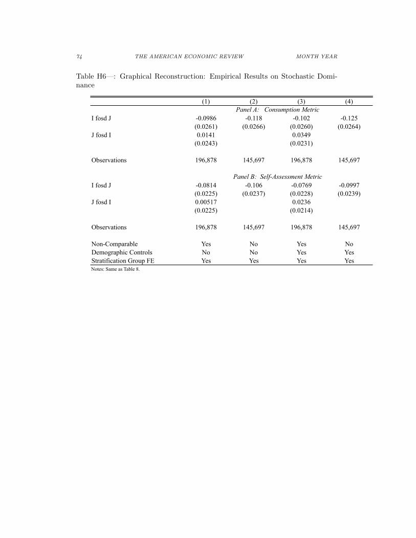
• Tables H4 and H6: Networks that tend to dominate other networks (inexpectation now since we are integrating over missing data) tend to havelower error rates, both when we look at the synthetic outcome data as wellas in the empirical data.
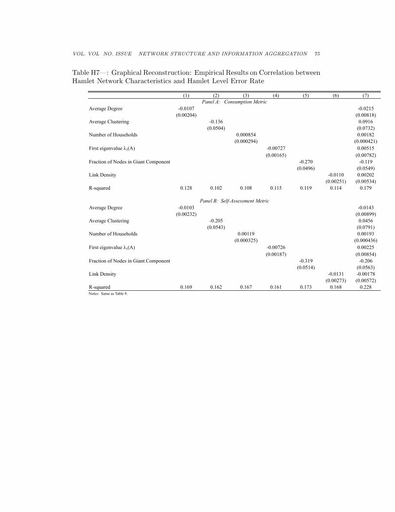
• Tables H5 and H7: Both in the simulations and in the empirical data wesee that a higher degree reduces error rates, more clustering reduces errorrates, a higher first eigenvalue reduces error rates, and a higher densityreduces error rates. When looking at the moments conditional on eachother, the average degree and the share of nodes in the giant componentrobustly matter in the simulations and in the data. Note a difference oncewe correct for sampling: the average degree no longer has the “wrong” sign.
• Tables H8 and H9: Both show that community targeting is differentiallymore effective relative to the PMT in more diffusive hamlets. Therefore,the main result of Section V is largely unchanged when we integrate overthe missing data.
In sum, correcting for missing data in this way leaves the main results of thepaper intact.

VOL. VOL NO. ISSUE NETWORK STRUCTURE AND INFORMATION AGGREGATION 69
Table H1—: Graphical Reconstruction: The Correlation between Household Net-work Characteristics and the Error Rate in Ranking Income Status of Household
(1) (2) (3) (4) (5) (6) (7) (8)
Degree -0.00806 -0.00835 -0.00180 -0.00169(0.00113) (0.00133) (0.000632) (0.000984)
Clustering -0.0714 -0.0705 -0.0109 -0.0140(0.0171) (0.0162) (0.0106) (0.0115)
Eigenvector Centrality -0.103 0.0582 -0.0650 -0.0137(0.0505) (0.0586) (0.0273) (0.0407)
R-squared 0.028 0.006 0.003 0.034 0.667 0.667 0.667 0.667
Degree -0.0100 -0.0102 -0.00276 -0.00218(0.00130) (0.00154) (0.000748) (0.00133)
Clustering -0.0875 -0.0843 0.00286 -0.000613(0.0186) (0.0175) (0.0126) (0.0138)
Eigenvector Centrality -0.143 0.0533 -0.0921 -0.0310(0.0572) (0.0664) (0.0325) (0.0546)
R-squared 0.035 0.008 0.004 0.042 0.671 0.670 0.671 0.671
Degree -0.0118 -0.0122 -0.00275 -0.00202(0.00133) (0.00157) (0.000652) (0.00106)
Clustering -0.0985 -0.0963 -0.00115 -0.00381(0.0218) (0.0205) (0.0130) (0.0139)
Eigenvector Centrality -0.142 0.0903 -0.0978 -0.0409(0.0575) (0.0667) (0.0304) (0.0466)
R-squared 0.051 0.010 0.004 0.060 0.712 0.711 0.712 0.712
Hamlet Fixed Effect No No No No Yes Yes Yes YesNotes: Same as Table 2.
Panel B: Self-Assessment Metric, Error Rate
Panel A: Consumption Metric, Error Rate
Panel C: Share of Don't Knows

70 THE AMERICAN ECONOMIC REVIEW MONTH YEAR
Table H2—: Graphical Reconstruction: The Correlation between Household Net-work Characteristics and the Error Rate in Ranking Income Status of Households
(1) (2) (3) (4) (5) (6) (7) (8)
Degree -0.00700 -0.00723 -0.00134 -0.00125(0.00109) (0.00130) (0.000632) (0.000977)
Clustering -0.0563 -0.0567 -0.01000 -0.0122(0.0165) (0.0159) (0.0105) (0.0114)
Eigenvector Centrality -0.0985 0.0388 -0.0500 -0.0116(0.0494) (0.0581) (0.0272) (0.0405)
R-squared 0.046 0.029 0.028 0.050 0.671 0.670 0.671 0.671
Degree -0.00835 -0.00842 -0.00214 -0.00161(0.00125) (0.00150) (0.000738) (0.00131)
Clustering -0.0643 -0.0618 0.00373 0.00139(0.0179) (0.0171) (0.0123) (0.0135)
Eigenvector Centrality -0.136 0.0215 -0.0717 -0.0273(0.0554) (0.0653) (0.0319) (0.0538)
R-squared 0.069 0.049 0.049 0.072 0.676 0.675 0.676 0.676
Degree -0.00975 -0.0101 -0.00205 -0.00126(0.00121) (0.00147) (0.000614) (0.00104)
Clustering -0.0649 -0.0654 0.00288 0.00181(0.0201) (0.0193) (0.0128) (0.0137)
Eigenvector Centrality -0.129 0.0547 -0.0751 -0.0405(0.0543) (0.0647) (0.0301) (0.0472)
R-squared 0.099 0.069 0.068 0.103 0.72 0.72 0.72 0.72
Hamlet Fixed Effect No No No No Yes Yes Yes YesNotes: Same as Table 3.
Panel B: Self-Assessment Metric, Error Rate
Panel A: Consumption Metric, Error Rate
Panel C: Share of Don't Knows
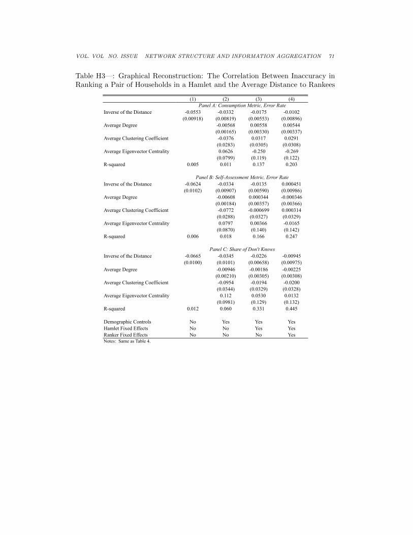
VOL. VOL NO. ISSUE NETWORK STRUCTURE AND INFORMATION AGGREGATION 71
Table H3—: Graphical Reconstruction: The Correlation Between Inaccuracy inRanking a Pair of Households in a Hamlet and the Average Distance to Rankees
(1) (2) (3) (4)
Inverse of the Distance -0.0553 -0.0332 -0.0175 -0.0102(0.00918) (0.00819) (0.00553) (0.00896)
Average Degree -0.00568 0.00558 0.00544(0.00165) (0.00330) (0.00337)
Average Clustering Coefficient -0.0376 0.0317 0.0291(0.0283) (0.0305) (0.0308)
Average Eigenvector Centrality 0.0626 -0.250 -0.269(0.0799) (0.119) (0.122)
R-squared 0.005 0.011 0.137 0.203
Inverse of the Distance -0.0624 -0.0334 -0.0135 0.000451(0.0102) (0.00907) (0.00590) (0.00986)
Average Degree -0.00608 0.000344 -0.000346(0.00184) (0.00357) (0.00366)
Average Clustering Coefficient -0.0772 -0.000699 0.000314(0.0288) (0.0327) (0.0329)
Average Eigenvector Centrality 0.0797 0.00366 -0.0165(0.0870) (0.140) (0.142)
R-squared 0.006 0.018 0.166 0.247
Inverse of the Distance -0.0665 -0.0345 -0.0226 -0.00945(0.0100) (0.0101) (0.00658) (0.00975)
Average Degree -0.00946 -0.00186 -0.00225(0.00210) (0.00305) (0.00308)
Average Clustering Coefficient -0.0954 -0.0194 -0.0200(0.0344) (0.0329) (0.0328)
Average Eigenvector Centrality 0.112 0.0530 0.0132(0.0981) (0.129) (0.132)
R-squared 0.012 0.060 0.331 0.445
Demographic Controls No Yes Yes YesHamlet Fixed Effects No No Yes YesRanker Fixed Effects No No No YesNotes: Same as Table 4.
Panel A: Consumption Metric, Error Rate
Panel B: Self-Assessment Metric, Error Rate
Panel C: Share of Don't Knows

72 THE AMERICAN ECONOMIC REVIEW MONTH YEAR
Table H4—: Graphical Reconstruction: Numerical Predictions on StochasticDominance
(1) (2) (3) (4)
I fosd J -0.126 -0.224 -0.105 -0.190(0.0305) (0.0293) (0.0307) (0.0309)
J fosd I 0.0938 0.0971(0.0313) (0.0307)
Observations 193,753 143,161 193,753 143,161
Non-Comparable Yes No Yes NoDemographic Controls No No Yes YesStratification Group FE Yes Yes Yes YesNotes: Same as Table 6.

VOL. VOL NO. ISSUE NETWORK STRUCTURE AND INFORMATION AGGREGATION 73
Table H5—: Graphical Reconstruction: Numerical Predictions on Correlationbetween Hamlet Network Characteristics and Hamlet Level Error Rate
(1) (2) (3) (4) (5) (6) (7)
Average Degree -0.0205 0.0456(0.00399) (0.0131)
Average Clustering -0.237 0.348(0.0571) (0.0999)
Number of Households 0.000347 8.05e-07(0.000282) (0.000437)
First eigenvalue λ1(A) -0.0180 -0.0319(0.00318) (0.00623)
Fraction of Nodes in Giant Component -0.346 -0.655(0.0487) (0.0787)
Link Density -0.292 -0.248(0.0834) (0.133)
R-squared 0.440 0.423 0.401 0.451 0.482 0.415 0.534Notes: Same as Table 7.
74 THE AMERICAN ECONOMIC REVIEW MONTH YEAR
Table H6—: Graphical Reconstruction: Empirical Results on Stochastic Domi-nance
(1) (2) (3) (4)
I fosd J -0.0986 -0.118 -0.102 -0.125(0.0261) (0.0266) (0.0260) (0.0264)
J fosd I 0.0141 0.0349(0.0243) (0.0231)
Observations 196,878 145,697 196,878 145,697
I fosd J -0.0814 -0.106 -0.0769 -0.0997(0.0225) (0.0237) (0.0228) (0.0239)
J fosd I 0.00517 0.0236(0.0225) (0.0214)
Observations 196,878 145,697 196,878 145,697
Non-Comparable Yes No Yes NoDemographic Controls No No Yes YesStratification Group FE Yes Yes Yes YesNotes: Same as Table 8.
Panel B: Self-Assessment Metric
Panel A: Consumption Metric
VOL. VOL NO. ISSUE NETWORK STRUCTURE AND INFORMATION AGGREGATION 75
Table H7—: Graphical Reconstruction: Empirical Results on Correlation betweenHamlet Network Characteristics and Hamlet Level Error Rate
(1) (2) (3) (4) (5) (6) (7)
Average Degree -0.0107 -0.0215(0.00204) (0.00818)
Average Clustering -0.136 0.0916(0.0504) (0.0732)
Number of Households 0.000854 0.00182(0.000294) (0.000421)
First eigenvalue λ1(A) -0.00727 0.00515(0.00165) (0.00782)
Fraction of Nodes in Giant Component -0.270 -0.119(0.0496) (0.0549)
Link Density -0.0110 0.00202(0.00251) (0.00534)
R-squared 0.128 0.102 0.108 0.115 0.119 0.114 0.179
Average Degree -0.0103 -0.0143(0.00232) (0.00899)
Average Clustering -0.205 0.0456(0.0543) (0.0791)
Number of Households 0.00119 0.00193(0.000325) (0.000436)
First eigenvalue λ1(A) -0.00726 0.00225(0.00187) (0.00854)
Fraction of Nodes in Giant Component -0.319 -0.206(0.0514) (0.0563)
Link Density -0.0131 -0.00178(0.00273) (0.00572)
R-squared 0.169 0.162 0.167 0.161 0.173 0.168 0.228Notes: Same as Table 9.
Panel A: Consumption Metric
Panel B: Self-Assessment Metric

76 THE AMERICAN ECONOMIC REVIEW MONTH YEAR
Table H8—: Graphical Reconstruction: Rank Correlation on Targeting TypeInteracted with Diffusiveness (Principal Component)
(1) (2) (3) (4) (5) (6)
Community x Diffusiveness -0.0680 -0.0686 -0.0940 -0.0936(0.119) (0.119) (0.124) (0.126)
Hybrid x Diffusiveness -0.0425 -0.0452 -0.0632(0.116) (0.117) (0.126)
Community -0.0563 -0.0217 -0.0176 -0.00804 -0.00370(0.0321) (0.0652) (0.0651) (0.0677) (0.0678)
Hybrid -0.0627 -0.0362 -0.0314 -0.0180(0.0330) (0.0683) (0.0688) (0.0760)
Diffusiveness -0.0143 0.0119 0.0730 0.0973 0.0727(0.0755) (0.0781) (0.0929) (0.105) (0.0927)
(Community or Hybrid) x Diffusiveness -0.0766(0.104)
(Community or Hybrid) -0.0134(0.0597)
R-squared 0.014 0.009 0.013 0.095 0.152 0.095
Community x Diffusiveness 0.198 0.197 0.156 0.143(0.113) (0.113) (0.119) (0.121)
Hybrid x Diffusiveness 0.184 0.181 0.152(0.114) (0.115) (0.123)
Community 0.111 0.0181 0.0250 0.0464 0.0503(0.0324) (0.0682) (0.0676) (0.0710) (0.0724)
Hybrid 0.0851 -0.00459 0.00276 0.0185(0.0334) (0.0702) (0.0703) (0.0775)
Diffusiveness -0.195 -0.149 -0.164 -0.158 -0.162(0.0808) (0.0832) (0.101) (0.110) (0.100)
(Community or Hybrid) x Diffusiveness 0.148(0.105)
(Community or Hybrid) 0.0355(0.0643)
R-squared 0.033 0.030 0.044 0.137 0.176 0.135
Stratification Group FE No No No Yes Yes YesDemographic Covariates No No No Yes Yes YesNotes: Same as Table 10.
Panel A: Rank Correlation (Consumption)
Panel B: Rank Correlation (Self-Assessment)

VOL. VOL NO. ISSUE NETWORK STRUCTURE AND INFORMATION AGGREGATION 77
Table H9—: Graphical Reconstruction: Rank Correlation on Targeting TypeInteracted with Diffusiveness (1 - Simulated Error Rate)
(1) (2) (3) (4) (5) (6)
Community x Diffusiveness 0.0472 0.0228 0.0224 0.0506(0.110) (0.114) (0.116) (0.104)
Hybrid x Diffusiveness 0.0249 -0.0352 -0.0476(0.109) (0.112) (0.114)
Community -0.0563 -0.0744 -0.0672 -0.0722 -0.0587(0.0321) (0.0636) (0.0665) (0.0686) (0.0618)
Hybrid -0.0627 -0.0708 -0.0422 -0.0296(0.0330) (0.0592) (0.0619) (0.0638)
Diffusiveness -0.0736 -0.0132 -0.00715 -0.0380 -0.00746(0.0733) (0.0841) (0.0854) (0.0700) (0.0851)
(Community or Hybrid) x Diffusiveness -0.0135(0.0977)
(Community or Hybrid) -0.0503(0.0558)
R-squared 0.014 0.015 0.083 0.091 0.086 0.090
Community x Diffusiveness 0.256 0.260 0.280 0.174(0.118) (0.121) (0.124) (0.105)
Hybrid x Diffusiveness 0.246 0.22 0.195(0.118) (0.117) (0.119)
Community 0.111 -0.0170 -0.0209 -0.0305 -0.0264(0.0324) (0.0662) (0.0682) (0.0706) (0.0598)
Hybrid 0.0851 -0.0311 -0.0199 -0.00324(0.0334) (0.0653) (0.0665) (0.0687)
Diffusiveness -0.269 -0.257 -0.251 -0.14 -0.250(0.0837) (0.0984) (0.102) (0.0775) (0.101)
(Community or Hybrid) x Diffusiveness 0.236(0.106)
(Community or Hybrid) -0.0162(0.0608)
R-squared 0.033 0.050 0.115 0.135 0.117 0.133
Stratification Group FE No No No Yes Yes YesDemographic Covariates No No No Yes Yes YesNotes: Same as Table 11.
Panel A: Rank Correlation (Consumption)
Panel B: Rank Correlation (Self-Assessment)

78 THE AMERICAN ECONOMIC REVIEW MONTH YEAR
Augmenting Network Data
Another approach to investigating the degree to which the missing data is anissue is to collect new data. Since one might be concerned about the missing 10percent of kinship links, particularly since they are a non-random set, we decidedto collect new data.
To investigate the degree to which this is an issue, we randomly selected 10 vil-lages in Java, and went back and revisited these villages in the field. In these 10villages, we obtained data on links in the study hamlet through a key informantsurvey: we sat with the neighborhood head, his spouse, and/or another local lead-ers who the neighborhood head viewed as knowledgeable about the community.We then walked them through the full list of households one by one, and askedhim to enumerate the full set of kin links for the entire network in the hamlet.On average, this procedure took 1.6 hours per village.
Why is this useful? From our previous discussion, we know that we are missingabout 10% of our kinship links. Returning to the field allows us to attempt to“fill in” these links, though we do again stress that we likely have information on90% of the potential kinship links.
Of course, since we enlist the neighborhood head to go through and enumerateeveryone’s kin, surely he wouldn’t do a complete enumeration. He does a goodjob though: 74% of the kin he named were indeed kin in our baseline and at thesame time, for each individual who we directly surveyed, he named about 1/3 oftheir kin. This suggests that he isn’t adding much noise but at the same timewill help us get about a 1/3 of the missing 10%. In short, this exercise puts us athaving 93% of our kinship data.
For these 10 hamlets, we now augment our old kinship data with the new data.We then conduct two exercises. First, we use this augmented network directly.That is, we add any links that were reported in 2015 but not in 2007. Second, wecompute the network using this augmented data but only using the augmentedinformation on those individuals who we would have observed under our oldsampling scheme. This means that we are not updating the links for someonewho was not directly survey nor named in any of the listing exercises.
Taken together, both of these exercises holds the data fixed (augments the 2007sample with the 2015 update) but varies the sampling scheme. We then comparethe results to the original datasets. We expect that little should change giventhat we went from having about 90% of links to 93% of links.
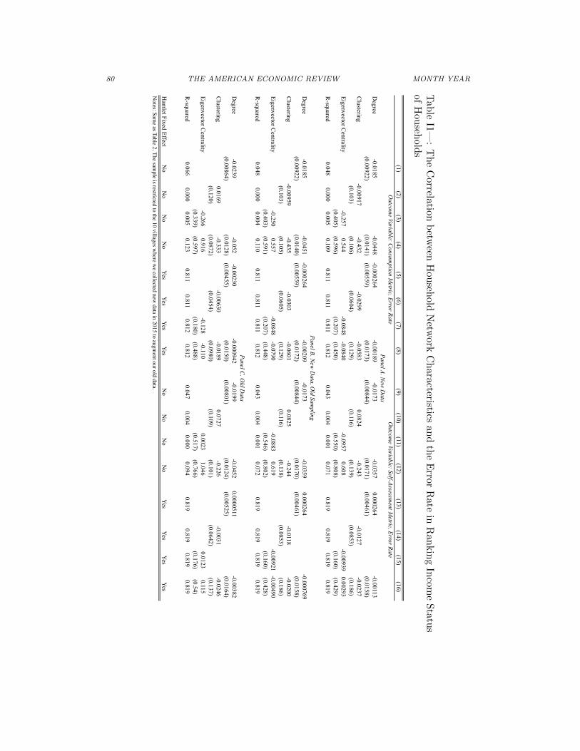
Specifically, we replicate the within-village regressions (Tables 2, 3, and 4) usingthese two sets of networks. We do not replicate the cross-village regressions sincewe only have the new complete data for 10 hamlets. These are shown below, inTables I1-I3.
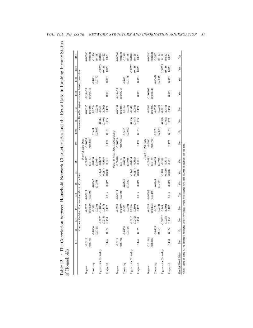
What is apparent from these tables is that, holding the data fixed, samplingmakes virtually no difference.
Let us discuss Table I1 in detail, but the reader can easily verify that thesame is true turning to Table I2 (which just includes demographic covariates)

VOL. VOL NO. ISSUE NETWORK STRUCTURE AND INFORMATION AGGREGATION 79
and Table I3 (which looks at distance of ranker to rankees). Columns 1-8 usethe 2015-augmented kinship data, Columns 7-16 use the 2015-augmented data,restricted to our previous sample, and Columns 17-24 use our original 2007 data.For example, when we compare columns 1, 9 and 17 we see that the results arenearly identical when we look at the degree of the ranking household. Similarly,looking at columns 4, 12, and 20 shows that even when we take degree, cluster-ing and centrality conditional on each other, the results are qualitatively (andquantitatively) very similar.
In general, by comparing columns x, x+8 and x+16 in Tables I1 and I2 orcolumns x, x+4 and x+8 in Table I3, we can see that the results are essentiallyidentical when we use the full dataset and when we use the same data but onlyinformation on the nodes we sample and very similar to our original data. Asdiscussed above, we believe that at an intuitive level the reason the sampling doesnot change the results is that (i) we already had complete kinship data on almost70 percent of the network, (ii) for the nodes we are particularly interested in, wehad an even higher proportion of the links, and (iii) we nearly had 90 percent ofall kinship links overall.
80 THE AMERICAN ECONOMIC REVIEW MONTH YEAR
Tab
leI1
—:
Th
eC
orrelation
betw
eenH
ouseh
oldN
etwork
Ch
aracteristicsan
dth
eE
rrorR
atein
Ran
kin
gIn
come
Statu
sof
Hou
sehold
s
(1)(2)
(3)(4)
(5)(6)
(7)(8)
(9)(10)
(11)(12)
(13)(14)
(15)(16)
Degree
-0.0185-0.0448
-0.000264-0.00189
-0.0173-0.0357
0.000264-0.00113
(0.00922)(0.0141)
(0.00559)(0.0173)
(0.00844)(0.0171)
(0.00461)(0.0158)
Clustering
-0.00917-0.432
-0.0299-0.0583
0.0824-0.243
-0.0127-0.0237
(0.103)(0.106)
(0.0604)(0.129)
(0.116)(0.139)
(0.0853)(0.186)
Eigenvector Centrality
-0.2570.544
-0.0848-0.0840
-0.09570.608
-0.009390.00293
(0.405)(0.596)
(0.207)(0.450)
(0.550)(0.808)
(0.160)(0.429)
R-squared
0.0480.000
0.0050.109
0.8110.811
0.8110.812
0.0430.004
0.0010.071
0.8190.819
0.8190.819
Degree
-0.0185-0.0451
-0.000264-0.00209
-0.0173-0.0359
0.000264-0.000769
(0.00922)(0.0140)
(0.00559)(0.0172)
(0.00844)(0.0170)
(0.00461)(0.0158)
Clustering
-0.00959-0.435
-0.0303-0.0601
0.0825-0.244
-0.0118-0.0200
(0.103)(0.105)
(0.0605)(0.129)
(0.116)(0.138)
(0.0853)(0.186)
Eigenvector Centrality
-0.2500.557
-0.0848-0.0790
-0.08830.619
-0.00921-0.00490
(0.403)(0.591)
(0.207)(0.448)
(0.546)(0.802)
(0.160)(0.428)
R-squared
0.0480.000
0.0040.110
0.8110.811
0.8110.812
0.0430.004
0.0010.072
0.8190.819
0.8190.819
Degree
-0.0239-0.052
-0.00230-0.000942
-0.0199-0.0452
0.0000511-0.00382
(0.00864)(0.0128)
(0.00455)(0.0150)
(0.00801)(0.0124)
(0.00525)(0.0164)
Clustering
0.0169-0.333
-0.00630-0.0189
0.0727-0.226
-0.0031-0.0246
(0.120)(0.0872)
(0.0454)(0.0980)
(0.109)(0.101)
(0.0642)(0.137)
Eigenvector Centrality
-0.2660.916
-0.128-0.110
0.00231.046
0.01230.115
(0.339)(0.597)
(0.180)(0.488)
(0.517)(0.766)
(0.176)(0.54)
R-squared
0.0660.000
0.0050.123
0.8110.811
0.8120.812
0.0470.004
0.0000.094
0.8190.819
0.8190.819
Ham
let Fixed EffectN
oN
oN
oN
oYes
YesYes
YesN
oN
oN
oN
oYes
YesYes
Yes
Panel A. New
Data
Panel B. New
Data, O
ld Sampling
Panel C. O
ld Data
Notes: Sam
e as Table 2. The sample is restricted to the 10 villages w
here we collected new
data in 2015 to augment our old data.
Outcom
e Variable: Self-Assessment M
etric, Error RateO
utcome Variable: C
onsumption M
etric, Error Rate
VOL. VOL NO. ISSUE NETWORK STRUCTURE AND INFORMATION AGGREGATION 81
Tab
leI2
—:
Th
eC
orre
lati
on
bet
wee
nH
ou
seh
old
Net
wor
kC
har
acte
rist
ics
and
the
Err
orR
ate
inR
ankin
gIn
com
eS
tatu
sof
Hou
seh
old
s
(1)
(2)
(3)
(4)
(5)
(6)
(7)
(8)
(9)
(10)
(11)
(12)
(13)
(14)
(15)
(16)
Deg
ree
-0.0111
-0.0275
-0.00113
-0.00397
-0.00828
0.00215
-9.58e-05
-0.00246
(0.00701)
(0.0270)
(0.00558)
(0.0133)
(0.00690)
(0.0286)
(0.00430)
(0.0154)
Clu
ster
ing
-0.0556
-0.318
-0.0342
-0.0834
0.0411
0.0206
-0.0131
-0.0354
(0.0786)
(0.210)
(0.0578)
(0.0954)
(0.0933)
(0.234)
(0.0770)
(0.168)
Eige
nvec
tor C
entra
lity
-0.587*
-0.00436
-0.144
-0.0973
-0.514
-0.562
-0.0265
0.0186
(0.285)
(0.817)
(0.217)
(0.393)
(0.494)
(1.092)
(0.148)
(0.422)
R-s
quar
ed0.146
0.134
0.154
0.177
0.819
0.819
0.820
0.821
0.170
0.163
0.179
0.179
0.823
0.823
0.823
0.823
Deg
ree
-0.0111
-0.0281
-0.00113
-0.00419
-0.00828
0.00181
-9.58e-05
-0.00209
(0.00701)
(0.0269)
(0.00558)
(0.0131)
(0.00690)
(0.0286)
(0.00430)
(0.0153)
Clu
ster
ing
-0.0558
-0.323
-0.0346
-0.0854
0.0416
0.0194
-0.0121
-0.0316
(0.0786)
(0.210)
(0.0580)
(0.0948)
(0.0932)
(0.235)
(0.0771)
(0.168)
Eige
nvec
tor C
entra
lity
-0.581*
0.0194
-0.143
-0.0914
-0.506
-0.546
-0.0262
0.0106
(0.282)
(0.809)
(0.217)
(0.392)
(0.489)
(1.086)
(0.148)
(0.421)
R-s
quar
ed0.146
0.135
0.154
0.177
0.819
0.819
0.820
0.821
0.170
0.163
0.179
0.179
0.823
0.823
0.823
0.823
Deg
ree
-0.0166*
-0.0387
-0.00302
-0.00315
-0.0100
-0.0109
-0.000167
-0.00580
(0.00890)
(0.0402)
(0.00455)
(0.0139)
(0.00790)
(0.0386)
(0.00444)
(0.0162)
Clu
ster
ing
-0.0365
-0.274
-0.0164
-0.0438
0.0174
-0.0555
-0.00659
-0.0405
(0.104)
(0.212)
(0.0474)
(0.0945)
(0.0873)
(0.227)
(0.0525)
(0.117)
Eige
nvec
tor C
entra
lity
-0.589**
0.449
-0.181
-0.108
-0.390
-0.0910
0.00263
0.158
(0.220)
(1.300)
(0.190)
(0.511)
(0.467)
(1.416)
(0.145)
(0.512)
R-s
quar
ed0.158
0.134
0.155
0.182
0.819
0.819
0.820
0.821
0.172
0.163
0.172
0.174
0.823
0.823
0.823
0.823
Ham
let F
ixed
Effe
ctN
oN
oN
oN
oYe
sYe
sYe
sYe
sN
oN
oN
oN
oYe
sYe
sYe
sYe
sN
otes
: Sa
me
as T
able
3. T
he sa
mpl
e is
rest
ricte
d to
the
10 v
illag
es w
here
we
colle
cted
new
dat
a in
201
5 to
aug
men
t our
old
dat
a.
Out
com
e Va
riab
le: C
onsu
mpt
ion
Met
ric,
Err
or R
ate
Out
com
e Va
riab
le: S
elf-A
sses
smen
t Met
ric,
Err
or R
ate
Pane
l A. N
ew D
ata
Pane
l B. N
ew D
ata,
Old
Sam
plin
g
Pane
l C. O
ld D
ata
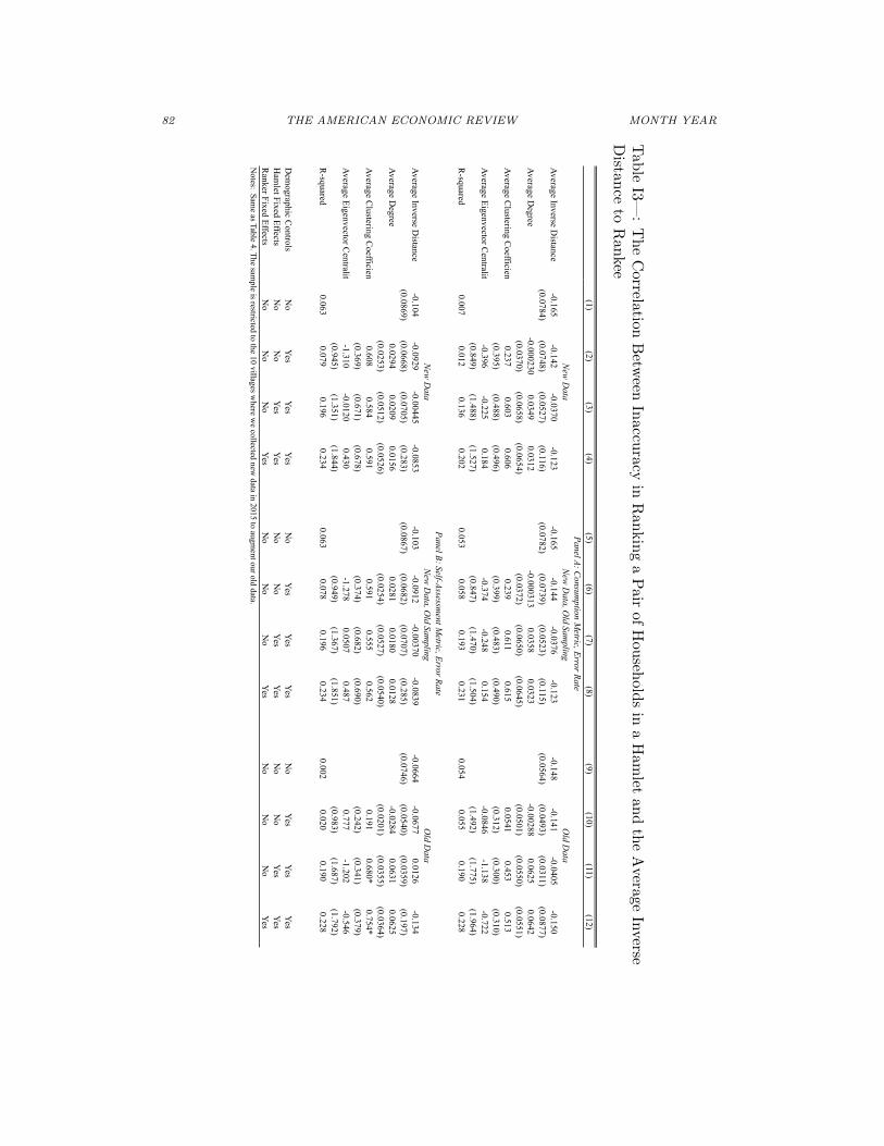
82 THE AMERICAN ECONOMIC REVIEW MONTH YEAR
Tab
leI3—
:T
he
Correlation
Betw
eenIn
accuracy
inR
ankin
ga
Pair
ofH
ouseh
olds
ina
Ham
letan
dth
eA
verageIn
verse
Distan
ceto
Ran
kee
(1)(2)
(3)(4)
(5)(6)
(7)(8)
(9)(10)
(11)(12)
Average Inverse Distance
-0.165-0.142
-0.0370-0.123
-0.165-0.144
-0.0376-0.123
-0.148-0.141
-0.0405-0.150
(0.0784)(0.0748)
(0.0527)(0.116)
(0.0782)(0.0739)
(0.0523)(0.115)
(0.0564)(0.0493)
(0.0311)(0.0877)
Average Degree
-0.0002300.0349
0.0312-0.000313
0.03580.0323
-0.002880.0625
0.0642(0.0370)
(0.0658)(0.0654)
(0.0372)(0.0650)
(0.0645)(0.0501)
(0.0550)(0.0551)
Average Clustering C
oefficient0.237
0.6030.606
0.2390.611
0.6150.0541
0.4530.513
(0.395)(0.488)
(0.496)(0.399)
(0.483)(0.490)
(0.312)(0.300)
(0.310)Average Eigenvector C
entrality-0.396
-0.2250.184
-0.374-0.248
0.154-0.0846
-1.138-0.722
(0.849)(1.488)
(1.527)(0.847)
(1.470)(1.504)
(1.492)(1.775)
(1.964)R
-squared0.007
0.0120.136
0.2020.053
0.0580.193
0.2310.054
0.0550.190
0.228
Average Inverse Distance
-0.104-0.0929
-0.00445-0.0853
-0.103-0.0912
-0.00370-0.0839
-0.0664-0.0677
0.0126-0.134
(0.0869)(0.0668)
(0.0705)(0.283)
(0.0867)(0.0682)
(0.0707)(0.285)
(0.0746)(0.0540)
(0.0359)(0.197)
Average Degree
0.02940.0209
0.01560.0281
0.01800.0128
-0.02840.0631
0.0625(0.0253)
(0.0512)(0.0526)
(0.0254)(0.0527)
(0.0540)(0.0201)
(0.0355)(0.0364)
Average Clustering C
oefficient0.608
0.5840.591
0.5910.555
0.5620.191
0.680*0.754*
(0.369)(0.671)
(0.678)(0.374)
(0.682)(0.690)
(0.242)(0.341)
(0.379)Average Eigenvector C
entrality-1.310
-0.01200.430
-1.2780.0507
0.4870.777
-1.202-0.546
(0.945)(1.351)
(1.844)(0.949)
(1.367)(1.851)
(0.983)(1.687)
(1.792)R
-squared0.063
0.0790.196
0.2340.063
0.0780.196
0.2340.002
0.0200.190
0.228
Dem
ographic Controls
No
YesYes
YesN
oYes
YesYes
No
YesYes
YesH
amlet Fixed Effects
No
No
YesYes
No
No
YesYes
No
No
YesYes
Ranker Fixed Effects
No
No
No
YesN
oN
oN
oYes
No
No
No
YesN
otes: Same as Table 4. The sam
ple is restricted to the 10 villages where w
e collected new data in 2015 to augm
ent our old data.
Panel A: Consum
ption Metric, Error Rate
Panel B: Self-Assessment M
etric, Error RateN
ew D
ataN
ew D
ata, Old Sam
plingO
ld Data
New
Data
New
Data, O
ld Sampling
Old D
ata
VOL. VOL NO. ISSUE NETWORK STRUCTURE AND INFORMATION AGGREGATION 83
Dropping Further Data
Here we show that, qualitatively, our results do not appear to get much worse ifwe were to use an even sparser network sampled in the same way. Specifically, weshow that neither dropping 25% of links randomly nor sampling 6 people insteadof 8 substantially alters our results. This, again, suggests that our results are nottoo sensitive to having a partial network structure.
In order to operationalize this, for each network we do the following.
• For b = 1, ..., B
– Exercise 1: drop 25% of links uniformly at random. This generates anew adjacency matrix Ab
r for each network r.
– Exercise 2: select two households (out of the surveyed households)uniformly at random and drop their links. Also drop their surveyresponses where they nominate the 5 poorest, 5 richest, and elites aswell as all of the kin of these folk. This generates a new adjacencymatrix Ab
r for each network r.
• For both exercises, construct regressors W(Abr
)for each draw for each
network and then construct an average, integrating over the missing data
E [W (Ar)] :=1
B
B∑b=1
W(Abr
)which we then use in our regressions.
In this way, we then rerun our analysis from the main part of the paper, con-structing regressors from this data, simulating the network learning process onthis subgraph, etc. The goal is to document that the qualitative results, in thiscase, are robust to this procedure. In practice we set B = 100.
J1. Dropping 25% of links uniformly at random
• Tables J1/J2:
We see that higher degree and more (eigenvector) central nodes have lowererror rates. Further, the results typically hold even when adding demo-graphic controls and are mostly robust to the inclusion of hamlet fixedeffects. This is consistent with our main results.
• Table J3:
When nodes are further on average from those whom they are ranking, theyare more likely to make a mistake. This is robust to including demographiccontrols and hamlet fixed effects. Again the results are underpowered withranker fixed effects. This is consistent with our main results.

84 THE AMERICAN ECONOMIC REVIEW MONTH YEAR
• Table J4:
Networks that have degree distributions that (first order stochastically)dominate other networks tend to have lower error rates. Again, this isconsistent with our main results.
• Table J5:
We find that a higher degree, more clustering, a higher first eigenvalue, anda higher density, all are associated with a lower error rate. This is consistentwith our main results.
• Tables J6 and J7:
Here we look at whether community targeting does better relative to PMTin more “diffusive” hamlets where this is computed either via principalcomponents (Table J6) or by using the simulated error rate in these hamlets(Table J7). We find that being in a more diffusive hamlet (or less error-prone hamlet under our model) corresponds to community targeting beingmore effective than the PMT. This is consistent with our main results.
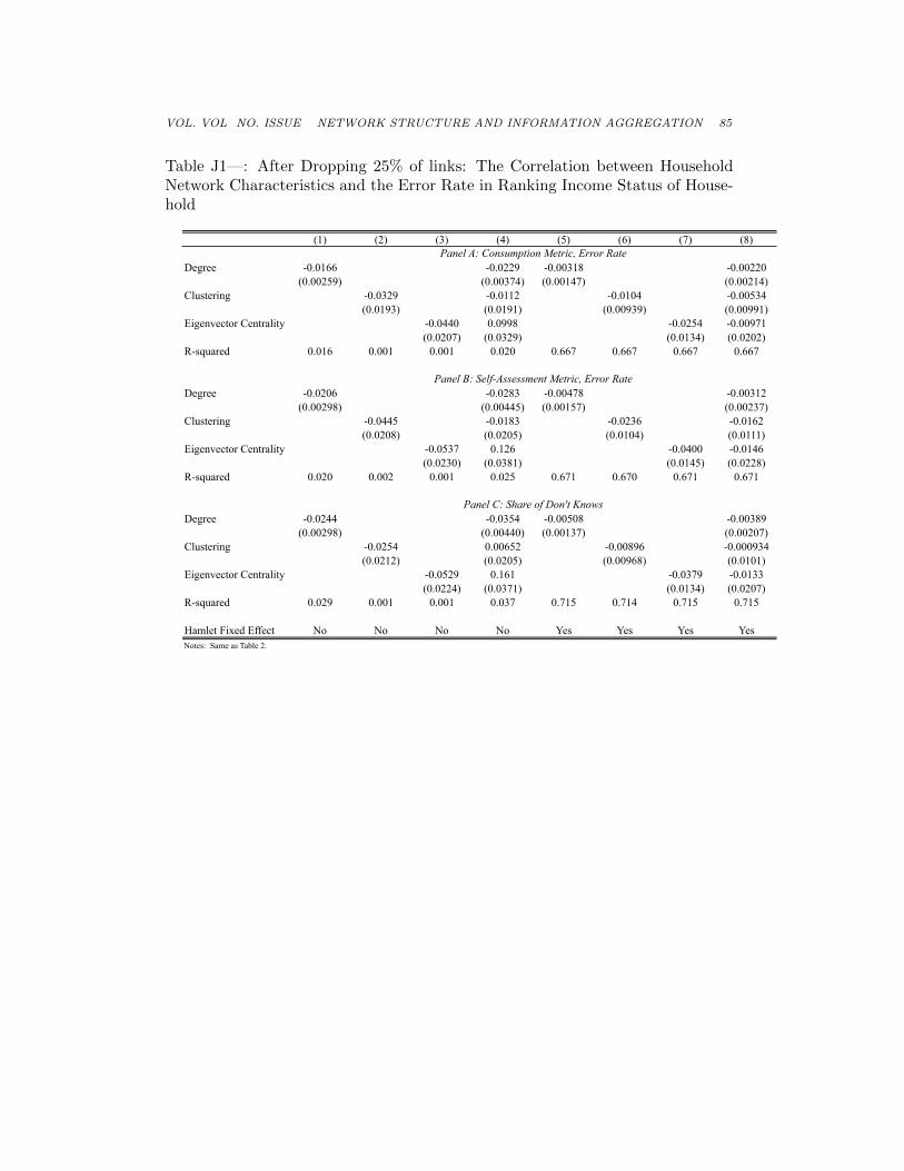
VOL. VOL NO. ISSUE NETWORK STRUCTURE AND INFORMATION AGGREGATION 85
Table J1—: After Dropping 25% of links: The Correlation between HouseholdNetwork Characteristics and the Error Rate in Ranking Income Status of House-hold
(1) (2) (3) (4) (5) (6) (7) (8)
Degree -0.0166 -0.0229 -0.00318 -0.00220(0.00259) (0.00374) (0.00147) (0.00214)
Clustering -0.0329 -0.0112 -0.0104 -0.00534(0.0193) (0.0191) (0.00939) (0.00991)
Eigenvector Centrality -0.0440 0.0998 -0.0254 -0.00971(0.0207) (0.0329) (0.0134) (0.0202)
R-squared 0.016 0.001 0.001 0.020 0.667 0.667 0.667 0.667
Degree -0.0206 -0.0283 -0.00478 -0.00312(0.00298) (0.00445) (0.00157) (0.00237)
Clustering -0.0445 -0.0183 -0.0236 -0.0162(0.0208) (0.0205) (0.0104) (0.0111)
Eigenvector Centrality -0.0537 0.126 -0.0400 -0.0146(0.0230) (0.0381) (0.0145) (0.0228)
R-squared 0.020 0.002 0.001 0.025 0.671 0.670 0.671 0.671
Degree -0.0244 -0.0354 -0.00508 -0.00389(0.00298) (0.00440) (0.00137) (0.00207)
Clustering -0.0254 0.00652 -0.00896 -0.000934(0.0212) (0.0205) (0.00968) (0.0101)
Eigenvector Centrality -0.0529 0.161 -0.0379 -0.0133(0.0224) (0.0371) (0.0134) (0.0207)
R-squared 0.029 0.001 0.001 0.037 0.715 0.714 0.715 0.715
Hamlet Fixed Effect No No No No Yes Yes Yes YesNotes: Same as Table 2.
Panel C: Share of Don't Knows
Panel A: Consumption Metric, Error Rate
Panel B: Self-Assessment Metric, Error Rate

86 THE AMERICAN ECONOMIC REVIEW MONTH YEAR
Table J2—: After Dropping 25% of links: The Correlation between HouseholdNetwork Characteristics and the Error Rate in Ranking Income Status of House-holds
(1) (2) (3) (4) (5) (6) (7) (8)
Degree -0.0138 -0.0186 -0.00221 -0.00153(0.00251) (0.00363) (0.00146) (0.00212)
Clustering -0.0281 -0.00986 -0.00887 -0.00550(0.0185) (0.0185) (0.00939) (0.00985)
Eigenvector Centrality -0.0408 0.0768 -0.0178 -0.00628(0.0203) (0.0320) (0.0133) (0.0201)
R-squared 0.037 0.027 0.027 0.039 0.671 0.671 0.671 0.671
Degree -0.0160 -0.0214 -0.00347 -0.00217(0.00291) (0.00433) (0.00156) (0.00237)
Clustering -0.0377 -0.0166 -0.0215 -0.0163(0.0196) (0.0194) (0.0105) (0.0112)
Eigenvector Centrality -0.0496 0.0875 -0.0299 -0.0105(0.0226) (0.0370) (0.0143) (0.0226)
R-squared 0.057 0.047 0.047 0.060 0.676 0.676 0.676 0.676
Degree -0.0188 -0.0270 -0.00371 -0.00252(0.00279) (0.00416) (0.00136) (0.00202)
Clustering -0.0173 0.00784 -0.00854 -0.00230(0.0195) (0.0191) (0.00979) (0.0101)
Eigenvector Centrality -0.0457 0.116 -0.0296 -0.0130(0.0213) (0.0357) (0.0134) (0.0204)
R-squared 0.083 0.066 0.067 0.088 0.723 0.722 0.723 0.723
Hamlet Fixed Effect No No No No Yes Yes Yes YesNotes: Same as Table 3.
Panel B: Self-Assessment Metric, Error Rate
Panel A: Consumption Metric, Error Rate
Panel B: Self-Assessment Metric, Error Rate
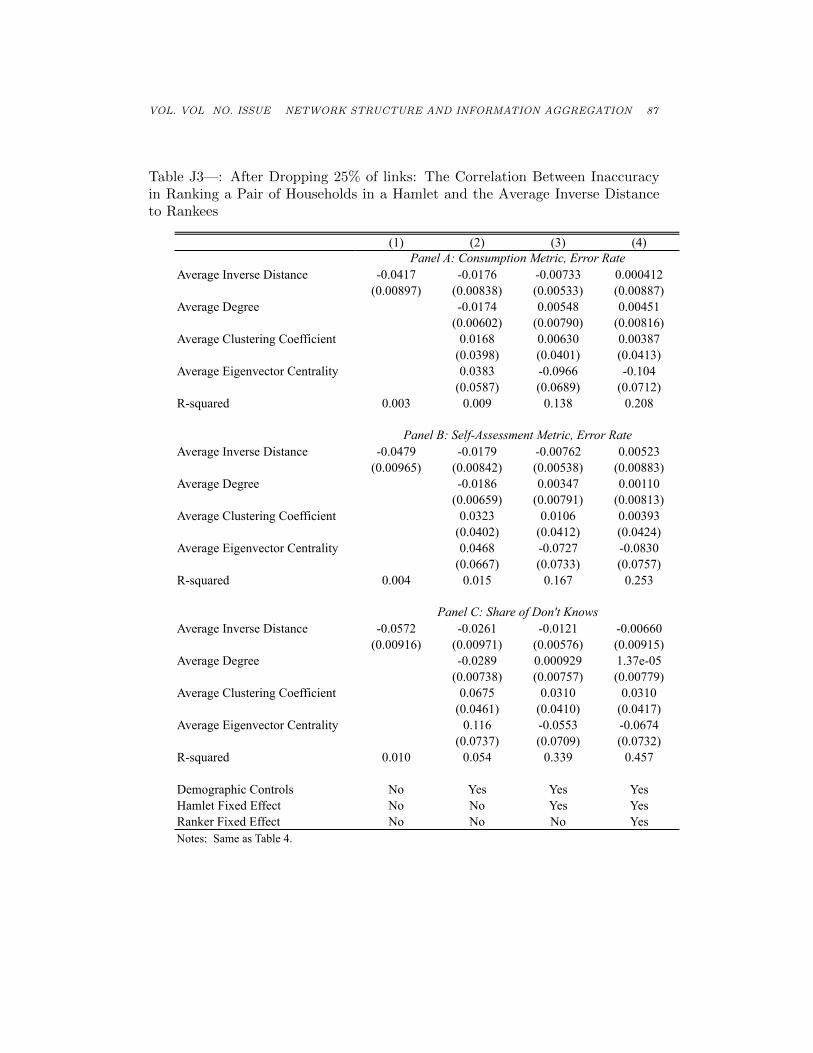
VOL. VOL NO. ISSUE NETWORK STRUCTURE AND INFORMATION AGGREGATION 87
Table J3—: After Dropping 25% of links: The Correlation Between Inaccuracyin Ranking a Pair of Households in a Hamlet and the Average Inverse Distanceto Rankees
(1) (2) (3) (4)
Average Inverse Distance -0.0417 -0.0176 -0.00733 0.000412(0.00897) (0.00838) (0.00533) (0.00887)
Average Degree -0.0174 0.00548 0.00451(0.00602) (0.00790) (0.00816)
Average Clustering Coefficient 0.0168 0.00630 0.00387(0.0398) (0.0401) (0.0413)
Average Eigenvector Centrality 0.0383 -0.0966 -0.104(0.0587) (0.0689) (0.0712)
R-squared 0.003 0.009 0.138 0.208
Average Inverse Distance -0.0479 -0.0179 -0.00762 0.00523(0.00965) (0.00842) (0.00538) (0.00883)
Average Degree -0.0186 0.00347 0.00110(0.00659) (0.00791) (0.00813)
Average Clustering Coefficient 0.0323 0.0106 0.00393(0.0402) (0.0412) (0.0424)
Average Eigenvector Centrality 0.0468 -0.0727 -0.0830(0.0667) (0.0733) (0.0757)
R-squared 0.004 0.015 0.167 0.253
Average Inverse Distance -0.0572 -0.0261 -0.0121 -0.00660(0.00916) (0.00971) (0.00576) (0.00915)
Average Degree -0.0289 0.000929 1.37e-05(0.00738) (0.00757) (0.00779)
Average Clustering Coefficient 0.0675 0.0310 0.0310(0.0461) (0.0410) (0.0417)
Average Eigenvector Centrality 0.116 -0.0553 -0.0674(0.0737) (0.0709) (0.0732)
R-squared 0.010 0.054 0.339 0.457
Demographic Controls No Yes Yes YesHamlet Fixed Effect No No Yes YesRanker Fixed Effect No No No YesNotes: Same as Table 4.
Panel A: Consumption Metric, Error Rate
Panel C: Share of Don't Knows
Panel B: Self-Assessment Metric, Error Rate

88 THE AMERICAN ECONOMIC REVIEW MONTH YEAR
Table J4—: After Dropping 25% of links: Empirical Results on Stochastic Dom-inance
(1) (2) (3) (4)
I fosd J -0.0968 -0.141 -0.0906 -0.124(0.0192) (0.0297) (0.0191) (0.0280)
J fosd I 0.0471 0.0484(0.0184) (0.0179)
I fosd J -0.102 -0.172 -0.0772 -0.125(0.0178) (0.0265) (0.0181) (0.0262)
J fosd I 0.0735 0.0593(0.0168) (0.0168)
Non-Comparable Yes No Yes NoDemographic Controls No No Yes YesStratification Group FE Yes Yes Yes YesNotes: Same as Table 8.
Panel B: Self-Assessment Metric
Panel A: Consumption Metric

VOL. VOL NO. ISSUE NETWORK STRUCTURE AND INFORMATION AGGREGATION 89
Table J5—: After Dropping 25% of links: Empirical Results on Correlation be-tween Hamlet Network Characteristics and Hamlet Level Error Rate
(1) (2) (3) (4) (5) (6) (7)
Average Degree -0.0313 0.0231(0.0134) (0.0393)
Average Clustering -0.223 0.0772(0.138) (0.258)
Number of Households 0.000762 0.000978(0.000398) (0.000422)
First eigenvalue λ1(A) -0.0222 -0.0407(0.00966) (0.0220)
Fraction of Nodes in Giant Component -0.106 -0.0264(0.0443) (0.0972)
Link Density -0.0355 0.00856(0.0188) (0.0329)
R-squared 0.248 0.244 0.249 0.249 0.249 0.247 0.257
Average Degree -0.0376 0.0228(0.0131) (0.0453)
Average Clustering -0.0424 0.515(0.132) (0.188)
Number of Households 0.00118 0.00137(0.000419) (0.000449)
First eigenvalue λ1(A) -0.0215 -0.0385(0.0101) (0.0238)
Fraction of Nodes in Giant Component -0.147 -0.0908(0.0437) (0.126)
Link Density -0.0327 -0.0124(0.0193) (0.0367)
R-squared 0.311 0.303 0.319 0.309 0.315 0.307 0.329Notes: Same as Table 9.
Panel A: Consumption Metric
Panel B: Self-Assessment Metric

90 THE AMERICAN ECONOMIC REVIEW MONTH YEAR
Table J6—: After Dropping 25% of links: Rank Correlation on Targeting TypeInteracted with Diffusiveness (Principal Component)
(1) (2) (3) (4) (5) (6)
Community x Diffusiveness -0.0444 -0.0512 -0.0947 -0.0866(0.119) (0.118) (0.124) (0.127)
Hybrid x Diffusiveness -0.0585 -0.0604 -0.0988(0.115) (0.115) (0.124)
Community -0.0563 -0.0392 -0.0322 -0.0160 -0.0162(0.0321) (0.0659) (0.0655) (0.0686) (0.0697)
Hybrid -0.0627 -0.0349 -0.0306 -0.00672(0.0330) (0.0671) (0.0674) (0.0739)
Diffusiveness -0.0355 -0.0116 0.0529 0.0764 0.0524(0.0787) (0.0802) (0.0933) (0.102) (0.0930)
(Community or Hybrid) x Diffusiveness -0.0956(0.105)
(Community or Hybrid) -0.0120(0.0599)
R-squared 0.014 0.012 0.016 0.095 0.151 0.094
Community x Diffusiveness 0.278 0.266 0.237 0.242(0.110) (0.108) (0.116) (0.120)
Hybrid x Diffusiveness 0.325 0.324 0.315(0.112) (0.111) (0.118)
Community 0.111 -0.0308 -0.0185 -0.00424 -0.00846(0.0324) (0.0659) (0.0649) (0.0696) (0.0718)
Hybrid 0.0851 -0.0842 -0.0777 -0.0731(0.0334) (0.0676) (0.0674) (0.0735)
Diffusiveness -0.267 -0.225 -0.222 -0.246 -0.221(0.0776) (0.0784) (0.0898) (0.0963) (0.0897)
(Community or Hybrid) x Diffusiveness 0.273(0.102)
(Community or Hybrid) -0.0358(0.0621)
R-squared 0.033 0.035 0.049 0.131 0.169 0.129
Stratification Group FE No No No Yes Yes YesDemographic Covariates No No No Yes Yes YesNotes: Same as Table 10.
Panel A: Rank Correlation (Consumption)
Panel B: Rank Correlation (Self-Assessment)
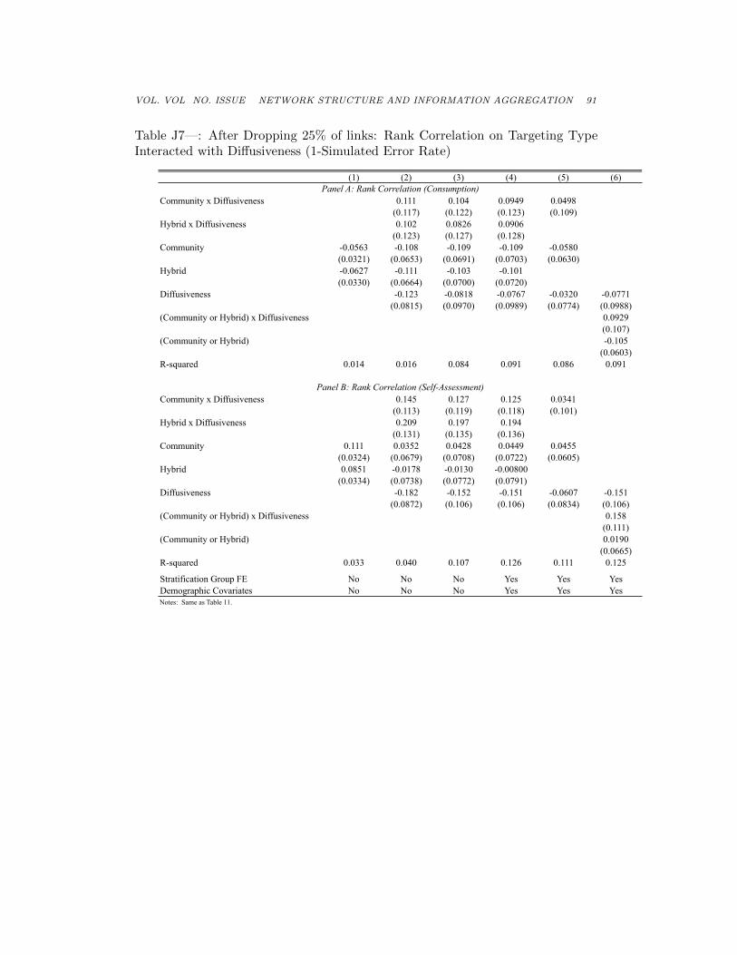
VOL. VOL NO. ISSUE NETWORK STRUCTURE AND INFORMATION AGGREGATION 91
Table J7—: After Dropping 25% of links: Rank Correlation on Targeting TypeInteracted with Diffusiveness (1-Simulated Error Rate)
(1) (2) (3) (4) (5) (6)
Community x Diffusiveness 0.111 0.104 0.0949 0.0498(0.117) (0.122) (0.123) (0.109)
Hybrid x Diffusiveness 0.102 0.0826 0.0906(0.123) (0.127) (0.128)
Community -0.0563 -0.108 -0.109 -0.109 -0.0580(0.0321) (0.0653) (0.0691) (0.0703) (0.0630)
Hybrid -0.0627 -0.111 -0.103 -0.101(0.0330) (0.0664) (0.0700) (0.0720)
Diffusiveness -0.123 -0.0818 -0.0767 -0.0320 -0.0771(0.0815) (0.0970) (0.0989) (0.0774) (0.0988)
(Community or Hybrid) x Diffusiveness 0.0929(0.107)
(Community or Hybrid) -0.105(0.0603)
R-squared 0.014 0.016 0.084 0.091 0.086 0.091
Community x Diffusiveness 0.145 0.127 0.125 0.0341(0.113) (0.119) (0.118) (0.101)
Hybrid x Diffusiveness 0.209 0.197 0.194(0.131) (0.135) (0.136)
Community 0.111 0.0352 0.0428 0.0449 0.0455(0.0324) (0.0679) (0.0708) (0.0722) (0.0605)
Hybrid 0.0851 -0.0178 -0.0130 -0.00800(0.0334) (0.0738) (0.0772) (0.0791)
Diffusiveness -0.182 -0.152 -0.151 -0.0607 -0.151(0.0872) (0.106) (0.106) (0.0834) (0.106)
(Community or Hybrid) x Diffusiveness 0.158(0.111)
(Community or Hybrid) 0.0190(0.0665)
R-squared 0.033 0.040 0.107 0.126 0.111 0.125
Stratification Group FE No No No Yes Yes YesDemographic Covariates No No No Yes Yes YesNotes: Same as Table 11.
Panel A: Rank Correlation (Consumption)
Panel B: Rank Correlation (Self-Assessment)

92 THE AMERICAN ECONOMIC REVIEW MONTH YEAR
J2. Dropping 2 sampled households and all of their information
• Tables J8/J9:
We see that higher degree and more (eigenvector) central nodes have lowererror rates. Further, the results typically hold even when adding demo-graphic controls and are mostly robust to the inclusion of hamlet fixedeffects. This is consistent with our main results.
• Table J10:
When nodes are further on average from those whom they are ranking, theyare more likely to make a mistake. This is robust to including demographiccontrols and hamlet fixed effects. Again the results are underpowered withranker fixed effects. This is consistent with our main results.
• Table J11:
Networks that have degree distributions that (first order stochastically)dominate other networks tend to have lower error rates. Again, this isconsistent with our main results.
• Table J12:
We find that a higher degree reduces error rates, more clustering reduceserror rates, a higher first eigenvalue reduces error rates, and a higher densityreduces error rates. This is consistent with our main results.
• Tables J13 and J14:
Here we look at whether community targeting does better relative to PMTin more “diffusive” villages where this is computed either via principal com-ponents (Table J13) or by using the simulated error rate in these hamlets(Table J14). We find that being in a more diffusive hamlet (or less error-prone hamlet under our model) corresponds to community targeting beingmore effective than the PMT. This is consistent with our main results.

VOL. VOL NO. ISSUE NETWORK STRUCTURE AND INFORMATION AGGREGATION 93
Table J8—: Dropping Two Households: The Correlation between Household Net-work Characteristics and the Error Rate in Ranking Income Status of Household
(1) (2) (3) (4) (5) (6) (7) (8)
Degree -0.0118 -0.0140 -0.00324 -0.00190(0.00135) (0.00199) (0.000896) (0.00172)
Clustering -0.0394 -0.0390 -0.0101 -0.00803(0.0164) (0.0166) (0.0103) (0.0137)
Eigenvector Centrality -0.181 0.124 -0.0877 -0.0486(0.0384) (0.0585) (0.0273) (0.0519)
R-squared 0.046 0.003 0.011 0.050 0.690 0.688 0.690 0.690
Degree -0.0136 -0.0168 -0.00320 -0.00157(0.00155) (0.00227) (0.00103) (0.00196)
Clustering -0.0283 -0.0313 -0.00668 -0.00335(0.0176) (0.0173) (0.0113) (0.0142)
Eigenvector Centrality -0.183 0.170 -0.0875 -0.0569(0.0429) (0.0647) (0.0299) (0.0561)
R-squared 0.050 0.001 0.009 0.054 0.687 0.686 0.688 0.688
Degree -0.0161 -0.0188 -0.00451 0.000510(0.00160) (0.00228) (0.000931) (0.00159)
Clustering -0.0251 -0.0188 -0.000908 0.0156(0.0200) (0.0194) (0.0121) (0.0144)
Eigenvector Centrality -0.240 0.141 -0.147 -0.165(0.0457) (0.0657) (0.0284) (0.0481)
R-squared 0.072 0.001 0.016 0.075 0.732 0.729 0.733 0.733
Hamlet Fixed Effect No No No No Yes Yes Yes YesNotes: Same as Table 2.
Panel C: Share of Don't Knows
Panel A: Consumption Metric, Error Rate
Panel B: Self-Assessment Metric, Error Rate
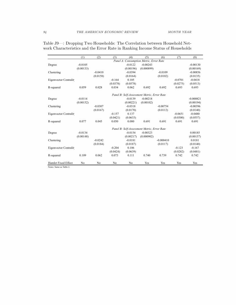
94 THE AMERICAN ECONOMIC REVIEW MONTH YEAR
Table J9—: Dropping Two Households: The Correlation between Household Net-work Characteristics and the Error Rate in Ranking Income Status of Households
(1) (2) (3) (4) (5) (6) (7) (8)
Degree -0.0105 -0.0122 -0.00243 -0.00130(0.00133) (0.00196) (0.000899) (0.00169)
Clustering -0.0410 -0.0394 -0.0109 -0.00856(0.0158) (0.0164) (0.0102) (0.0135)
Eigenvector Centrality -0.164 0.105 -0.0701 -0.0418(0.0378) (0.0578) (0.0275) (0.0513)
R-squared 0.059 0.028 0.034 0.062 0.692 0.692 0.693 0.693
Degree -0.0114 -0.0139 -0.00218 -0.000821(0.00152) (0.00221) (0.00102) (0.00194)
Clustering -0.0307 -0.0318 -0.00754 -0.00396(0.0167) (0.0170) (0.0112) (0.0140)
Eigenvector Centrality -0.157 0.137 -0.0651 -0.0480(0.0421) (0.0633) (0.0300) (0.0557)
R-squared 0.077 0.045 0.050 0.080 0.691 0.691 0.691 0.691
Degree -0.0134 -0.0154 -0.00323 0.00185(0.00148) (0.00217) (0.000902) (0.00157)
Clustering -0.0242 -0.0181 -0.000410 0.0181(0.0184) (0.0187) (0.0117) (0.0140)
Eigenvector Centrality -0.204 0.106 -0.123 -0.167(0.0424) (0.0639) (0.0282) (0.0481)
R-squared 0.109 0.062 0.073 0.111 0.740 0.739 0.742 0.742
Hamlet Fixed Effect No No No No Yes Yes Yes YesNotes: Same as Table 2.
Panel B: Self-Assessment Metric, Error Rate
Panel A: Consumption Metric, Error Rate
Panel B: Self-Assessment Metric, Error Rate

VOL. VOL NO. ISSUE NETWORK STRUCTURE AND INFORMATION AGGREGATION 95
Table J10—: Dropping Two Households: The Correlation Between Inaccuracy inRanking a Pair of Households in a Hamlet and the Average Inverse Distance toRankees
(1) (2) (3) (4)
Average Inverse Distance -0.0561 -0.0352 -0.0159 -0.00508(0.00925) (0.0103) (0.00749) (0.0155)
Average Degree -0.0106 -0.00149 -0.00132(0.00323) (0.00516) (0.00567)
Average Clustering Coefficient 0.0111 0.0287 0.0302(0.0340) (0.0405) (0.0438)
Average Eigenvector Centrality 0.184 0.166 0.117(0.0997) (0.121) (0.129)
R-squared 0.007 0.013 0.176 0.270
Average Inverse Distance -0.0706 -0.0331 -0.0210 0.00523(0.00990) (0.0104) (0.00796) (0.0146)
Average Degree -0.0134 -0.00741 -0.00740(0.00331) (0.00537) (0.00578)
Average Clustering Coefficient 0.0178 0.0292 0.0319(0.0363) (0.0406) (0.0433)
Average Eigenvector Centrality 0.118 0.176 0.0581(0.107) (0.128) (0.138)
R-squared 0.011 0.023 0.211 0.322
Average Inverse Distance -0.0707 -0.0406 -0.0186 0.00521(0.00964) (0.0118) (0.00845) (0.0138)
Average Degree -0.0154 -0.00492 -0.00427(0.00375) (0.00469) (0.00491)
Average Clustering Coefficient 0.0322 0.0102 0.0143(0.0391) (0.0379) (0.0391)
Average Eigenvector Centrality 0.235 0.207 0.0672(0.120) (0.123) (0.129)
R-squared 0.020 0.063 0.387 0.525
Demographic Controls No Yes Yes YesHamlet Fixed Effect No No Yes YesRanker Fixed Effect No No No YesNotes: Same as Table 4.
Panel A: Consumption Metric, Error Rate
Panel C: Share of Don't Knows
Panel B: Self-Assessment Metric, Error Rate

96 THE AMERICAN ECONOMIC REVIEW MONTH YEAR
Table J11—: Dropping Two Households: Empirical Results on Stochastic Domi-nance
(1) (2) (3) (4)
I fosd J -0.0987 -0.139 -0.0942 -0.120(0.0202) (0.0278) (0.0201) (0.0258)
J fosd I 0.0530 0.0577(0.0188) (0.0183)
I fosd J -0.108 -0.162 -0.0829 -0.111(0.0189) (0.0249) (0.0188) (0.0235)
J fosd I 0.0730 0.0601(0.0173) (0.0175)
Non-Comparable Yes No Yes NoDemographic Controls No No Yes YesStratification Group FE Yes Yes Yes YesNotes: Same as Table 8.
Panel B: Self-Assessment Metric
Panel A: Consumption Metric
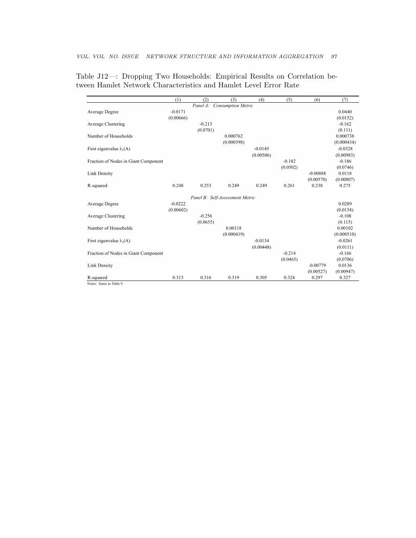
VOL. VOL NO. ISSUE NETWORK STRUCTURE AND INFORMATION AGGREGATION 97
Table J12—: Dropping Two Households: Empirical Results on Correlation be-tween Hamlet Network Characteristics and Hamlet Level Error Rate
(1) (2) (3) (4) (5) (6) (7)
Average Degree -0.0171 0.0440(0.00666) (0.0152)
Average Clustering -0.213 -0.162(0.0701) (0.111)
Number of Households 0.000762 0.000738(0.000398) (0.000434)
First eigenvalue λ1(A) -0.0145 -0.0328(0.00506) (0.00983)
Fraction of Nodes in Giant Component -0.182 -0.186(0.0502) (0.0746)
Link Density -0.00888 0.0118(0.00570) (0.00807)
R-squared 0.248 0.253 0.249 0.249 0.261 0.238 0.275
Average Degree -0.0222 0.0289(0.00602) (0.0154)
Average Clustering -0.256 -0.108(0.0655) (0.115)
Number of Households 0.00118 0.00102(0.000419) (0.000510)
First eigenvalue λ1(A) -0.0134 -0.0261(0.00448) (0.0111)
Fraction of Nodes in Giant Component -0.214 -0.166(0.0465) (0.0706)
Link Density -0.00779 0.0136(0.00527) (0.00947)
R-squared 0.313 0.316 0.319 0.305 0.324 0.297 0.327Notes: Same as Table 9.
Panel A: Consumption Metric
Panel B: Self-Assessment Metric

98 THE AMERICAN ECONOMIC REVIEW MONTH YEAR
Table J13—: Dropping Two Households: Rank Correlation on Targeting TypeInteracted with Diffusiveness (Principal Component)
(1) (2) (3) (4) (5) (6)
Community x Diffusiveness 0.0155 0.00927 0.00791 0.00322(0.117) (0.118) (0.124) (0.126)
Hybrid x Diffusiveness 0.0613 0.0563 0.0457(0.111) (0.112) (0.120)
Community -0.0563 -0.0678 -0.0613 -0.0673 -0.0602(0.0321) (0.0633) (0.0633) (0.0674) (0.0677)
Hybrid -0.0627 -0.0971 -0.0916 -0.0817(0.0330) (0.0636) (0.0642) (0.0716)
Diffusiveness -0.0889 -0.0668 -0.0138 -0.00728 -0.0133(0.0759) (0.0776) (0.0968) (0.112) (0.0965)
(Community or Hybrid) x Diffusiveness 0.0288(0.103)
(Community or Hybrid) -0.075(0.0581)
R-squared 0.014 0.012 0.015 0.089 0.150 0.089
Community x Diffusiveness 0.261 0.250 0.242 0.238(0.112) (0.112) (0.118) (0.120)
Hybrid x Diffusiveness 0.325 0.317 0.319(0.110) (0.110) (0.116)
Community 0.111 -0.0200 -0.00774 -0.00416 -0.00426(0.0324) (0.0665) (0.0661) (0.0694) (0.0711)
Hybrid 0.0851 -0.0834 -0.0738 -0.0757(0.0334) (0.0668) (0.0670) (0.0725)
Diffusiveness -0.245 -0.202 -0.226 -0.251 -0.221(0.0771) (0.0795) (0.103) (0.117) (0.103)
(Community or Hybrid) x Diffusiveness 0.277(0.102)
(Community or Hybrid) -0.0368(0.0612)
R-squared 0.033 0.035 0.047 0.132 0.167 0.130
Stratification Group FE No No No Yes Yes YesDemographic Covariates No No No Yes Yes YesNotes: Same as Table 10.
Panel A: Rank Correlation (Consumption)
Panel B: Rank Correlation (Self-Assessment)
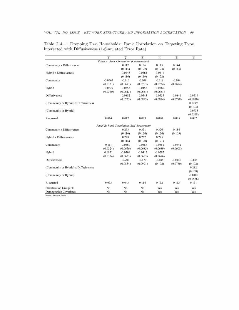
VOL. VOL NO. ISSUE NETWORK STRUCTURE AND INFORMATION AGGREGATION 99
Table J14—: Dropping Two Households: Rank Correlation on Targeting TypeInteracted with Diffusiveness (1-Simulated Error Rate)
(1) (2) (3) (4) (5) (6)
Community x Diffusiveness 0.117 0.106 0.115 0.144(0.115) (0.122) (0.123) (0.113)
Hybrid x Diffusiveness -0.0145 -0.0364 -0.0411(0.116) (0.119) (0.122)
Community -0.0563 -0.110 -0.109 -0.118 -0.104(0.0321) (0.0671) (0.0703) (0.0724) (0.0674)
Hybrid -0.0627 -0.0555 -0.0452 -0.0360(0.0330) (0.0613) (0.0631) (0.0651)
Diffusiveness -0.0882 -0.0543 -0.0535 -0.0846 -0.0514(0.0755) (0.0893) (0.0914) (0.0788) (0.0910)
(Community or Hybrid) x Diffusiveness 0.0299(0.103)
(Community or Hybrid) -0.0733(0.0568)
R-squared 0.014 0.017 0.083 0.090 0.085 0.087
Community x Diffusiveness 0.293 0.331 0.326 0.184(0.116) (0.124) (0.124) (0.105)
Hybrid x Diffusiveness 0.248 0.262 0.245(0.116) (0.120) (0.121)
Community 0.111 -0.0360 -0.0587 -0.0551 -0.0342(0.0324) (0.0656) (0.0685) (0.0689) (0.0608)
Hybrid 0.0851 -0.0309 -0.0415 -0.0282(0.0334) (0.0633) (0.0663) (0.0676)
Diffusiveness -0.209 -0.179 -0.188 -0.0446 -0.186(0.0854) (0.0991) (0.102) (0.0760) (0.102)
(Community or Hybrid) x Diffusiveness 0.282(0.108)
(Community or Hybrid) -0.0406(0.0586)
R-squared 0.033 0.043 0.114 0.132 0.113 0.131
Stratification Group FE No No No Yes Yes YesDemographic Covariates No No No Yes Yes YesNotes: Same as Table 11.
Panel A: Rank Correlation (Consumption)
Panel B: Rank Correlation (Self-Assessment)
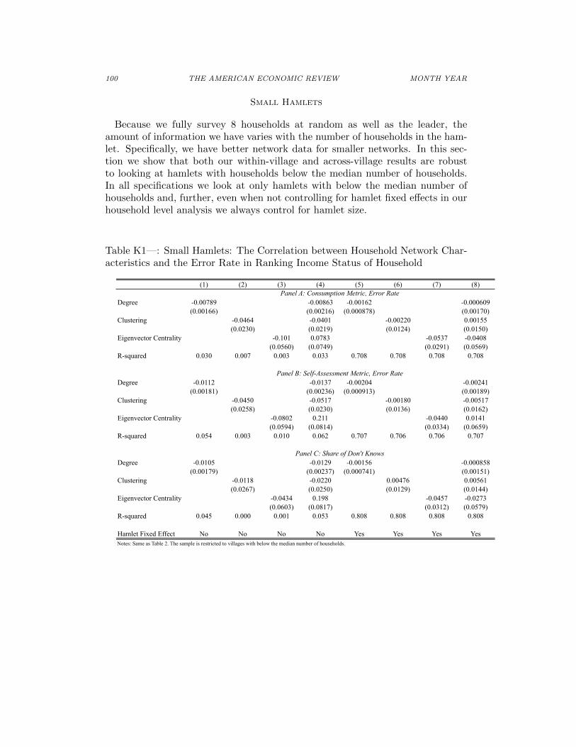
100 THE AMERICAN ECONOMIC REVIEW MONTH YEAR
Small Hamlets
Because we fully survey 8 households at random as well as the leader, theamount of information we have varies with the number of households in the ham-let. Specifically, we have better network data for smaller networks. In this sec-tion we show that both our within-village and across-village results are robustto looking at hamlets with households below the median number of households.In all specifications we look at only hamlets with below the median number ofhouseholds and, further, even when not controlling for hamlet fixed effects in ourhousehold level analysis we always control for hamlet size.
Table K1—: Small Hamlets: The Correlation between Household Network Char-acteristics and the Error Rate in Ranking Income Status of Household
(1) (2) (3) (4) (5) (6) (7) (8)
Degree -0.00789 -0.00863 -0.00162 -0.000609(0.00166) (0.00216) (0.000878) (0.00170)
Clustering -0.0464 -0.0401 -0.00220 0.00155(0.0230) (0.0219) (0.0124) (0.0150)
Eigenvector Centrality -0.101 0.0783 -0.0537 -0.0408(0.0560) (0.0749) (0.0291) (0.0569)
R-squared 0.030 0.007 0.003 0.033 0.708 0.708 0.708 0.708
Degree -0.0112 -0.0137 -0.00204 -0.00241(0.00181) (0.00236) (0.000913) (0.00189)
Clustering -0.0450 -0.0517 -0.00180 -0.00517(0.0258) (0.0230) (0.0136) (0.0162)
Eigenvector Centrality -0.0802 0.211 -0.0440 0.0141(0.0594) (0.0814) (0.0334) (0.0659)
R-squared 0.054 0.003 0.010 0.062 0.707 0.706 0.706 0.707
Degree -0.0105 -0.0129 -0.00156 -0.000858(0.00179) (0.00237) (0.000741) (0.00151)
Clustering -0.0118 -0.0220 0.00476 0.00561(0.0267) (0.0250) (0.0129) (0.0144)
Eigenvector Centrality -0.0434 0.198 -0.0457 -0.0273(0.0603) (0.0817) (0.0312) (0.0579)
R-squared 0.045 0.000 0.001 0.053 0.808 0.808 0.808 0.808
Hamlet Fixed Effect No No No No Yes Yes Yes YesNotes: Same as Table 2. The sample is restricted to villages with below the median number of households.
Panel C: Share of Don't Knows
Panel A: Consumption Metric, Error Rate
Panel B: Self-Assessment Metric, Error Rate

VOL. VOL NO. ISSUE NETWORK STRUCTURE AND INFORMATION AGGREGATION 101
Table K2—: Small Hamlets: The Correlation between Household Network Char-acteristics and the Error Rate in Ranking Income Status of Households
(1) (2) (3) (4) (5) (6) (7) (8)
Degree -0.00627 -0.00694 -0.00146 -0.000454(0.00151) (0.00202) (0.000873) (0.00168)
Clustering -0.0359 -0.0331 -0.00222 0.00156(0.0208) (0.0208) (0.0125) (0.0151)
Eigenvector Centrality -0.0826 0.0651 -0.0498 -0.0405(0.0530) (0.0741) (0.0295) (0.0572)
R-squared 0.045 0.032 0.032 0.047 0.709 0.709 0.709 0.709
Degree -0.00877 -0.0111 -0.00177 -0.00220(0.00162) (0.00218) (0.000905) (0.00187)
Clustering -0.0338 -0.0420 -0.00232 -0.00575(0.0222) (0.0218) (0.0135) (0.0161)
Eigenvector Centrality -0.0368 0.192 -0.0373 0.0160(0.0566) (0.0793) (0.0334) (0.0657)
R-squared 0.080 0.056 0.055 0.087 0.708 0.707 0.708 0.708
Degree -0.00790 -0.00979 -0.00148 -0.000715(0.00157) (0.00218) (0.000742) (0.00151)
Clustering -0.00649 -0.0145 0.00302 0.00427(0.0229) (0.0227) (0.0127) (0.0141)
Eigenvector Centrality -0.0330 0.147 -0.0460 -0.0306(0.0549) (0.0783) (0.0312) (0.0580)
R-squared 0.087 0.063 0.063 0.091 0.809 0.809 0.809 0.809
Hamlet Fixed Effect No No No No Yes Yes Yes YesNotes: Same as Table 3. The sample is restricted to villages with below the median number of households.
Panel C: Share of Don't Knows
Panel A: Consumption Metric, Error Rate
Panel B: Self-Assessment Metric, Error Rate

102 THE AMERICAN ECONOMIC REVIEW MONTH YEAR
Table K3—: Small Hamlets: The Correlation Between Inaccuracy in Ranking aPair of Households in a Hamlet and the Average Inverse Distance to Rankees
(1) (2) (3) (4)
Average Inverse Distance -0.0369 -0.0396 -0.0212 -0.0150(0.0122) (0.0116) (0.00792) (0.0208)
Average Degree -0.00298 0.00138 0.00190(0.00282) (0.00528) (0.00534)
Average Clustering Coefficient 0.0105 -0.0172 -0.0154(0.0393) (0.0455) (0.0458)
Average Eigenvector Centrality 0.143 0.00468 -0.0200(0.102) (0.177) (0.190)
R-squared 0.007 0.008 0.136 0.189
Average Inverse Distance -0.0335 -0.0361 -0.0187 -0.0131(0.0127) (0.0127) (0.00849) (0.0220)
Average Degree -0.00612 0.00313 0.00299(0.00286) (0.00592) (0.00602)
Average Clustering Coefficient 0.0129 0.0200 0.0216(0.0399) (0.0510) (0.0504)
Average Eigenvector Centrality 0.270 0.0287 0.0272(0.111) (0.211) (0.220)
R-squared 0.011 0.014 0.153 0.218
Average Inverse Distance -0.0509 -0.031 -0.0192 -0.0137(0.0143) (0.0148) (0.00963) (0.0216)
Average Degree -0.0102 -0.00778 -0.00696(0.00330) (0.00526) (0.00521)
Average Clustering Coefficient 0.0297 -0.0234 -0.0166(0.0450) (0.0461) (0.0453)
Average Eigenvector Centrality 0.260 0.300 0.263(0.122) (0.195) (0.210)
R-squared 0.008 0.044 0.339 0.414
Demographic Controls No Yes Yes YesHamlet Fixed Effect No No Yes YesRanker Fixed Effect No No No YesNotes: Same as Table 4. The sample is restricted to villages with below the median number of households.
Panel A: Consumption Metric, Error Rate
Panel C: Share of Don't Knows
Panel B: Self-Assessment Metric, Error Rate

VOL. VOL NO. ISSUE NETWORK STRUCTURE AND INFORMATION AGGREGATION 103
Table K4—: Small Hamlets: Empirical Results on Stochastic Dominance
(1) (2) (3) (4)
I fosd J -0.0476 -0.0145 -0.0630 -0.0395(0.00528) (0.00685) (0.00529) (0.00715)
J fosd I -0.0254 -0.00889(0.00617) (0.00601)
Observations 52,650 35,753 52,650 35,753
I fosd J -0.0773 -0.0853 -0.0890 -0.102(0.00551) (0.00620) (0.00544) (0.00640)
J fosd I 0.0145 0.0253(0.00555) (0.00556)
Observations 52,650 35,753 52,650 35,753
Non-Comparable Yes No Yes NoDemographic Controls No No Yes YesStratification Group FE Yes Yes Yes YesNotes: Same as Table 8. The sample is restricted to villages with below the median number of households.
Panel B: Self-Assessment Metric
Panel A: Consumption Metric

104 THE AMERICAN ECONOMIC REVIEW MONTH YEAR
Table K5—: Small Hamlets: Empirical Results on Correlation between HamletNetwork Characteristics and Hamlet Level Error Rate
(1) (2) (3) (4) (5) (6) (7)
Average Degree -0.0136 0.033(0.00387) (0.0173)
Average Clustering -0.314 -0.384(0.0652) (0.128)
Number of Households -0.000390 0.000752(0.00120) (0.00191)
First eigenvalue λ1(A) -0.0128 -0.0212(0.00343) (0.0108)
Fraction of Nodes in Giant Component -0.239 -0.195(0.0506) (0.0918)
Link Density -0.195 0.185(0.0905) (0.232)
R-squared 0.042 0.082 0.006 0.045 0.079 0.020 0.120
Average Degree -0.0219 0.0204(0.00395) (0.0183)
Average Clustering -0.464 -0.517(0.0674) (0.140)
Number of Households -0.000503 -0.000467(0.00137) (0.00195)
First eigenvalue λ1(A) -0.0188 -0.0130(0.00382) (0.0116)
Fraction of Nodes in Giant Component -0.333 -0.17(0.0523) (0.0981)
Link Density -0.344 0.211(0.0912) (0.230)
R-squared 0.092 0.153 0.011 0.083 0.133 0.051 0.182Notes: Same as Table 9. The sample is restricted to villages with below the median number of households.
Panel A: Consumption Metric
Panel B: Self-Assessment Metric

VOL. VOL NO. ISSUE NETWORK STRUCTURE AND INFORMATION AGGREGATION 105
Table K6—: Small Hamlets: Rank Correlation on Targeting Type Interacted withDiffusiveness (Principal Component)
(1) (2) (3) (4) (5) (6)
Community x Diffusiveness -0.168 -0.141 -0.0942 -0.104(0.163) (0.165) (0.183) (0.205)
Hybrid x Diffusiveness 0.0358 0.0534 0.0382(0.176) (0.177) (0.194)
Community -0.0471 0.0552 0.0380 0.00983 0.0445(0.0486) (0.0997) (0.101) (0.113) (0.126)
Hybrid -0.0311 -0.0518 -0.0632 -0.0368(0.0452) (0.122) (0.122) (0.136)
Diffusiveness -0.134 -0.100 -0.105 -0.103 -0.101(0.112) (0.117) (0.132) (0.170) (0.132)
(Community or Hybrid) x Diffusiveness -0.00939(0.161)
(Community or Hybrid) -0.0204(0.107)
R-squared 0.020 0.022 0.030 0.200 0.291 0.197
Community x Diffusiveness -0.0346 -9.09e-05 -0.0273 -0.0317(0.177) (0.178) (0.210) (0.223)
Hybrid x Diffusiveness 0.0382 0.0598 -0.0141(0.190) (0.191) (0.216)
Community 0.182 0.204 0.182 0.223 0.228(0.0448) (0.124) (0.124) (0.146) (0.158)
Hybrid 0.154 0.128 0.115 0.186(0.0464) (0.137) (0.137) (0.159)
Diffusiveness -0.0363 0.00625 -0.000961 -0.00352 -0.00159(0.133) (0.136) (0.164) (0.183) (0.163)
(Community or Hybrid) x Diffusiveness -0.0266(0.189)
(Community or Hybrid) 0.207(0.136)
R-squared 0.068 0.055 0.069 0.249 0.391 0.248
Stratification Group FE No No No Yes Yes YesDemographic Covariates No No No Yes Yes YesNotes: Same as Table 10. The sample is restricted to villages with below the median number of households.
Panel A: Rank Correlation (Consumption)
Panel B: Rank Correlation (Self-Assessment)

106 THE AMERICAN ECONOMIC REVIEW MONTH YEAR
Table K7—: Small Hamlets: Rank Correlation on Targeting Type Interacted withDiffusiveness (1-Simulated Error Rate)
(1) (2) (3) (4) (5) (6)
Community x Diffusiveness -0.0966 -0.0608 -0.0623 -0.0481(0.166) (0.186) (0.187) (0.158)
Hybrid x Diffusiveness -0.0315 -0.0167 -0.0175(0.150) (0.163) (0.164)
Community -0.0471 0.00818 -0.00632 -0.0173 -0.0122(0.0486) (0.0984) (0.109) (0.110) (0.101)
Hybrid -0.0311 -0.0115 -0.00276 -0.0124(0.0452) (0.0889) (0.0912) (0.0950)
Diffusiveness -0.0172 0.0598 0.0942 0.0755 0.0960(0.107) (0.145) (0.148) (0.107) (0.148)
(Community or Hybrid) x Diffusiveness -0.0341(0.150)
(Community or Hybrid) -0.0159(0.0841)
R-squared 0.020 0.023 0.177 0.198 0.197 0.196
Community x Diffusiveness -0.0498 0.00984 0.00759 -0.0503(0.157) (0.182) (0.188) (0.160)
Hybrid x Diffusiveness 0.0221 0.0559 0.0474(0.169) (0.178) (0.181)
Community 0.182 0.213 0.210 0.208 0.133(0.0448) (0.0919) (0.102) (0.107) (0.0969)
Hybrid 0.154 0.147 0.156 0.159(0.0464) (0.0967) (0.100) (0.101)
Diffusiveness -0.0675 -0.101 -0.123 -0.0259 -0.125(0.117) (0.148) (0.155) (0.123) (0.155)
(Community or Hybrid) x Diffusiveness 0.0291(0.161)
(Community or Hybrid) 0.181(0.0881)
R-squared 0.068 0.072 0.233 0.252 0.209 0.251
Stratification Group FE No No No Yes Yes YesDemographic Covariates No No No Yes Yes YesNotes: Same as Table 11. The sample is restricted to villages with below the median number of households.
Panel A: Rank Correlation (Consumption)
Panel B: Rank Correlation (Self-Assessment)

VOL. VOL NO. ISSUE NETWORK STRUCTURE AND INFORMATION AGGREGATION 107
Rural Sample
In this section we restrict our sample to only rural villages.
Table L1—: Rural Sample: The Correlation between Household Network Char-acteristics and the Error Rate in Ranking Income Status of Household
(1) (2) (3) (4) (5) (6) (7) (8)
Degree -0.00553 -0.00564 -0.00102 -0.00136(0.00130) (0.00167) (0.000818) (0.00143)
Clustering -0.0165 -0.0159 0.00632 0.00295(0.0201) (0.0195) (0.0126) (0.0133)
Eigenvector Centrality -0.111 0.00957 -0.0183 0.0169(0.0539) (0.0679) (0.0350) (0.0586)
R-squared 0.017 0.000 0.004 0.017 0.650 0.650 0.650 0.650
Degree -0.00826 -0.00870 -0.00223 -0.00219(0.00148) (0.00190) (0.000871) (0.00154)
Clustering -0.0177 -0.0192 0.0183 0.0139(0.0216) (0.0201) (0.0138) (0.0143)
Eigenvector Centrality -0.148 0.0364 -0.0502 0.00393(0.0605) (0.0756) (0.0364) (0.0595)
R-squared 0.031 0.000 0.006 0.031 0.647 0.646 0.646 0.647
Degree -0.0081 -0.00841 -0.00214 -0.000783(0.00124) (0.00157) (0.000725) (0.00123)
Clustering -0.0302 -0.0318 0.0101 0.0108(0.0211) (0.0205) (0.0142) (0.0156)
Eigenvector Centrality -0.158 0.0254 -0.0755 -0.0573(0.0523) (0.0642) (0.0323) (0.0501)
R-squared 0.042 0.002 0.010 0.044 0.708 0.707 0.708 0.709
Hamlet Fixed Effect No No No No Yes Yes Yes YesNotes: Same as Table 2. The sample is restricted to rural villages.
Panel C: Share of Don't Knows
Panel A: Consumption Metric, Error Rate
Panel B: Self-Assessment Metric, Error Rate
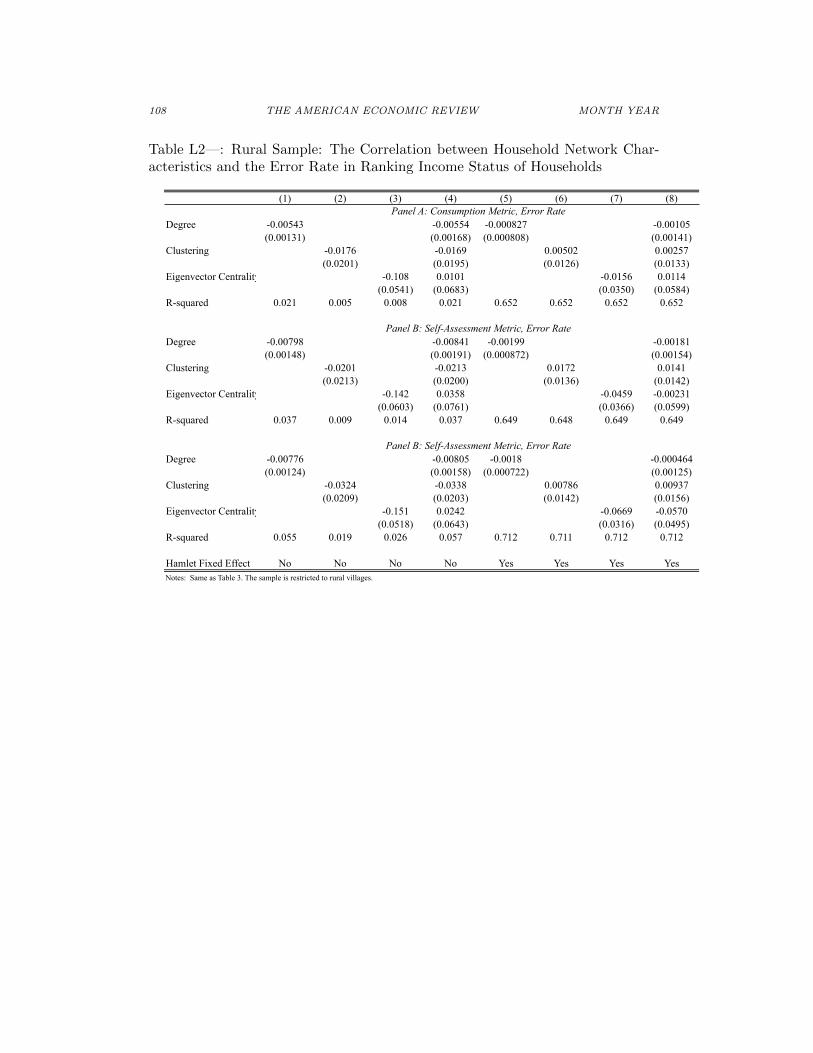
108 THE AMERICAN ECONOMIC REVIEW MONTH YEAR
Table L2—: Rural Sample: The Correlation between Household Network Char-acteristics and the Error Rate in Ranking Income Status of Households
(1) (2) (3) (4) (5) (6) (7) (8)
Degree -0.00543 -0.00554 -0.000827 -0.00105(0.00131) (0.00168) (0.000808) (0.00141)
Clustering -0.0176 -0.0169 0.00502 0.00257(0.0201) (0.0195) (0.0126) (0.0133)
Eigenvector Centrality -0.108 0.0101 -0.0156 0.0114(0.0541) (0.0683) (0.0350) (0.0584)
R-squared 0.021 0.005 0.008 0.021 0.652 0.652 0.652 0.652
Degree -0.00798 -0.00841 -0.00199 -0.00181(0.00148) (0.00191) (0.000872) (0.00154)
Clustering -0.0201 -0.0213 0.0172 0.0141(0.0213) (0.0200) (0.0136) (0.0142)
Eigenvector Centrality -0.142 0.0358 -0.0459 -0.00231(0.0603) (0.0761) (0.0366) (0.0599)
R-squared 0.037 0.009 0.014 0.037 0.649 0.648 0.649 0.649
Degree -0.00776 -0.00805 -0.0018 -0.000464(0.00124) (0.00158) (0.000722) (0.00125)
Clustering -0.0324 -0.0338 0.00786 0.00937(0.0209) (0.0203) (0.0142) (0.0156)
Eigenvector Centrality -0.151 0.0242 -0.0669 -0.0570(0.0518) (0.0643) (0.0316) (0.0495)
R-squared 0.055 0.019 0.026 0.057 0.712 0.711 0.712 0.712
Hamlet Fixed Effect No No No No Yes Yes Yes YesNotes: Same as Table 3. The sample is restricted to rural villages.
Panel B: Self-Assessment Metric, Error Rate
Panel A: Consumption Metric, Error Rate
Panel B: Self-Assessment Metric, Error Rate

VOL. VOL NO. ISSUE NETWORK STRUCTURE AND INFORMATION AGGREGATION 109
Table L3—: Rural Sample: The Correlation Between Inaccuracy in Ranking aPair of Households in a Hamlet and the Average Inverse Distance to Rankees
(1) (2) (3) (4)
Average Inverse Distance -0.0452 -0.0347 -0.0158 -0.00814(0.0114) (0.0114) (0.00714) (0.0155)
Average Degree -0.00407 0.00456 0.00445(0.00210) (0.00368) (0.00372)
Average Clustering Coefficient -0.00875 0.00357 0.00277(0.0361) (0.0357) (0.0358)
Average Eigenvector Centrality 0.0642 -0.0742 -0.0864(0.0920) (0.122) (0.127)
R-squared 0.007 0.007 0.125 0.186
Average Inverse Distance -0.0541 -0.0369 -0.0158 -0.0110(0.0126) (0.0130) (0.00804) (0.0176)
Average Degree -0.00642 0.00123 0.000993(0.00226) (0.00436) (0.00442)
Average Clustering Coefficient -0.0457 -0.0150 -0.00902(0.0400) (0.0438) (0.0440)
Average Eigenvector Centrality 0.126 0.0911 0.0737(0.107) (0.161) (0.161)
R-squared 0.010 0.012 0.153 0.230
Average Inverse Distance -0.0651 -0.0364 -0.0240 -0.00811(0.0142) (0.0132) (0.00878) (0.0161)
Average Degree -0.00955 -0.00112 -0.00104(0.00230) (0.00368) (0.00361)
Average Clustering Coefficient -0.0636 -0.0434 -0.0421(0.0425) (0.0397) (0.0394)
Average Eigenvector Centrality 0.145 0.103 0.0481(0.110) (0.143) (0.146)
R-squared 0.029 0.037 0.310 0.418
Demographic Controls No Yes Yes YesHamlet Fixed Effects No No Yes YesRanker Fixed Effects No No No YesNotes: Same as Table 4. The sample is restricted to rural villages.
Panel A: Consumption Metric, Error Rate
Panel C: Share of Don't Knows
Panel B: Self-Assessment Metric, Error Rate

110 THE AMERICAN ECONOMIC REVIEW MONTH YEAR
Table L4—: Rural Sample: Empirical Results on Stochastic Dominance
(1) (2) (3) (4)
I fosd J -0.0352 -0.0557 -0.0562 -0.0833(0.0278) (0.0412) (0.0270) (0.0386)
J fosd I 0.0177 0.0367(0.0256) (0.0240)
I fosd J -0.0625 -0.122 -0.0732 -0.135(0.0252) (0.0367) (0.0250) (0.0365)
J fosd I 0.0626 0.0757(0.0235) (0.0231)
Non-Comparable Yes No Yes NoDemographic Controls No No Yes YesStratification Group FE Yes Yes Yes YesNotes: Same as Table 8. The sample is restricted to rural villages.
Panel B: Self-Assessment Metric
Panel A: Consumption Metric

VOL. VOL NO. ISSUE NETWORK STRUCTURE AND INFORMATION AGGREGATION 111
Table L5—: Rural Sample: Empirical Results on Correlation between HamletNetwork Characteristics and Hamlet Level Error Rate
(1) (2) (3) (4) (5) (6) (7)
Average Degree -0.00599 0.00207(0.00342) (0.0206)
Average Clustering -0.105 -0.0626(0.0686) (0.155)
Number of Households -7.32e-05 -0.000155(0.000523) (0.000493)
First eigenvalue λ1(A) -0.00534 -0.00371(0.00331) (0.0120)
Fraction of Nodes in Giant Component -0.0988 -0.122(0.0554) (0.108)
Link Density -0.0347 0.168(0.0983) (0.198)
R-squared 0.173 0.173 0.167 0.174 0.177 0.168 0.170
Average Degree -0.0118 0.000302(0.00393) (0.0214)
Average Clustering -0.239 -0.263(0.0842) (0.192)
Number of Households 0.000264 -6.49e-05(0.000568) (0.000607)
First eigenvalue λ1(A) -0.00882 -0.00361(0.00323) (0.0117)
Fraction of Nodes in Giant Component -0.171 -0.0917(0.0614) (0.113)
Link Density -0.135 0.293(0.0891) (0.177)
R-squared 0.239 0.245 0.222 0.236 0.244 0.225 0.228Notes: Same as Table 9. The sample is restricted to rural villages.
Panel A: Consumption Metric
Panel B: Self-Assessment Metric

112 THE AMERICAN ECONOMIC REVIEW MONTH YEAR
Table L6—: Rural Sample: Rank Correlation on Targeting Type Interacted withDiffusiveness (Principal Component)
(1) (2) (3) (4) (5) (6)
Community x Diffusiveness -0.117 -0.117 -0.105 -0.163(0.194) (0.194) (0.201) (0.205)
Hybrid x Diffusiveness -0.267 -0.267 -0.309(0.181) (0.181) (0.205)
Community -0.0816 -0.0132 -0.0132 -0.0340 0.0183(0.0507) (0.126) (0.126) (0.136) (0.139)
Hybrid -0.0775 0.0876 0.0876 0.0933(0.0486) (0.122) (0.122) (0.141)
Diffusiveness 0.0494 0.0494 0.0904 0.136 0.0906(0.133) (0.133) (0.152) (0.172) (0.152)
(Community or Hybrid) x Diffusiveness -0.210(0.178)
(Community or Hybrid) 0.0294(0.123)
R-squared 0.010 0.021 0.021 0.168 0.211 0.164
Community x Diffusiveness 0.205 0.205 0.120 0.0375(0.181) (0.181) (0.185) (0.197)
Hybrid x Diffusiveness 0.110 0.110 0.106(0.187) (0.187) (0.186)
Community 0.114 -0.00460 -0.00460 0.0394 0.0891(0.0476) (0.125) (0.125) (0.127) (0.137)
Hybrid 0.0835 0.0159 0.0159 0.0213(0.0486) (0.130) (0.130) (0.129)
Diffusiveness -0.0585 -0.0585 0.0141 0.0765 0.0145(0.137) (0.137) (0.146) (0.161) (0.145)
(Community or Hybrid) x Diffusiveness 0.111(0.161)
(Community or Hybrid) 0.0306(0.112)
R-squared 0.018 0.023 0.023 0.172 0.213 0.171
Stratification Group FE No No No Yes Yes YesDemographic Covariates No No No Yes Yes YesNotes: Same as Table 10. The sample is restricted to rural villages.
Panel A: Rank Correlation (Consumption)
Panel B: Rank Correlation (Self-Assessment)

VOL. VOL NO. ISSUE NETWORK STRUCTURE AND INFORMATION AGGREGATION 113
Table L7—: Rural Sample: Rank Correlation on Targeting Type Interacted withDiffusiveness (1-Simulated Error Rate)
(1) (2) (3) (4) (5) (6)
Community x Diffusiveness 0.256 0.239 0.270 0.233(0.168) (0.186) (0.193) (0.163)
Hybrid x Diffusiveness 0.147 0.0770 0.0811(0.158) (0.182) (0.187)
Community -0.0816 -0.205 -0.213 -0.240 -0.168(0.0507) (0.0983) (0.107) (0.112) (0.0995)
Hybrid -0.0775 -0.143 -0.127 -0.140(0.0486) (0.0970) (0.105) (0.107)
Diffusiveness -0.165 -0.0715 -0.0620 -0.0496 -0.0639(0.111) (0.143) (0.147) (0.108) (0.147)
(Community or Hybrid) x Diffusiveness 0.168(0.166)
(Community or Hybrid) -0.186(0.0935)
R-squared 0.010 0.016 0.139 0.168 0.156 0.164
Community x Diffusiveness 0.175 0.132 0.108 0.188(0.179) (0.185) (0.193) (0.160)
Hybrid x Diffusiveness -0.0935 -0.0847 -0.160(0.187) (0.195) (0.191)
Community 0.114 0.0220 0.0544 0.0589 -0.0346(0.0476) (0.104) (0.103) (0.110) (0.0926)
Hybrid 0.0835 0.147 0.146 0.182*(0.0486) (0.105) (0.109) (0.106)
Diffusiveness -0.0818 -0.0434 0.00794 -0.0457 0.00448(0.136) (0.160) (0.161) (0.128) (0.160)
(Community or Hybrid) x Diffusiveness -0.0362(0.170)
(Community or Hybrid) 0.125(0.0949)
R-squared 0.017 0.028 0.146 0.187 0.172 0.179
Stratification Group FE No No No Yes Yes YesDemographic Covariates No No No Yes Yes YesNotes: Same as Table 11. The sample is restricted to rural villages.
Panel A: Rank Correlation (Consumption)
Panel B: Rank Correlation (Self-Assessment)
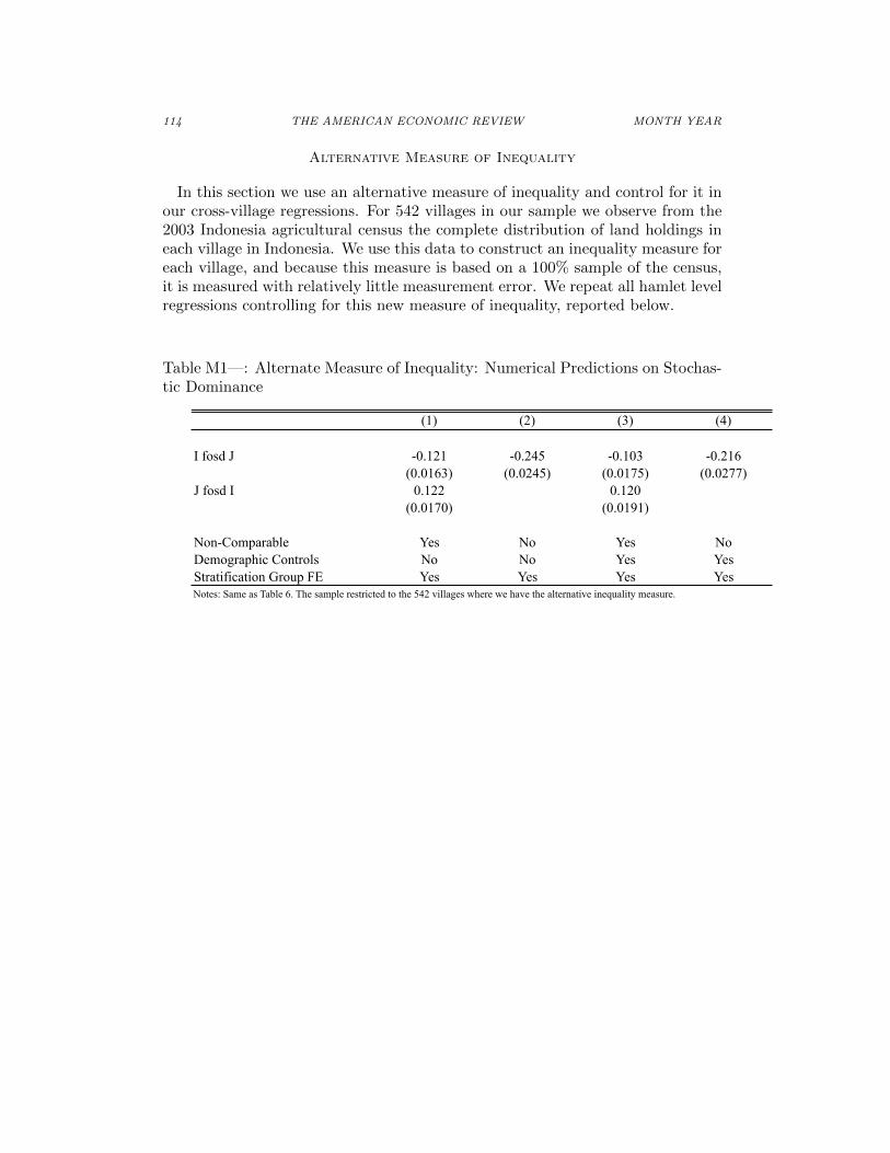
114 THE AMERICAN ECONOMIC REVIEW MONTH YEAR
Alternative Measure of Inequality
In this section we use an alternative measure of inequality and control for it inour cross-village regressions. For 542 villages in our sample we observe from the2003 Indonesia agricultural census the complete distribution of land holdings ineach village in Indonesia. We use this data to construct an inequality measure foreach village, and because this measure is based on a 100% sample of the census,it is measured with relatively little measurement error. We repeat all hamlet levelregressions controlling for this new measure of inequality, reported below.
Table M1—: Alternate Measure of Inequality: Numerical Predictions on Stochas-tic Dominance
(1) (2) (3) (4)
I fosd J -0.121 -0.245 -0.103 -0.216(0.0163) (0.0245) (0.0175) (0.0277)
J fosd I 0.122 0.120(0.0170) (0.0191)
Non-Comparable Yes No Yes NoDemographic Controls No No Yes YesStratification Group FE Yes Yes Yes YesNotes: Same as Table 6. The sample restricted to the 542 villages where we have the alternative inequality measure.
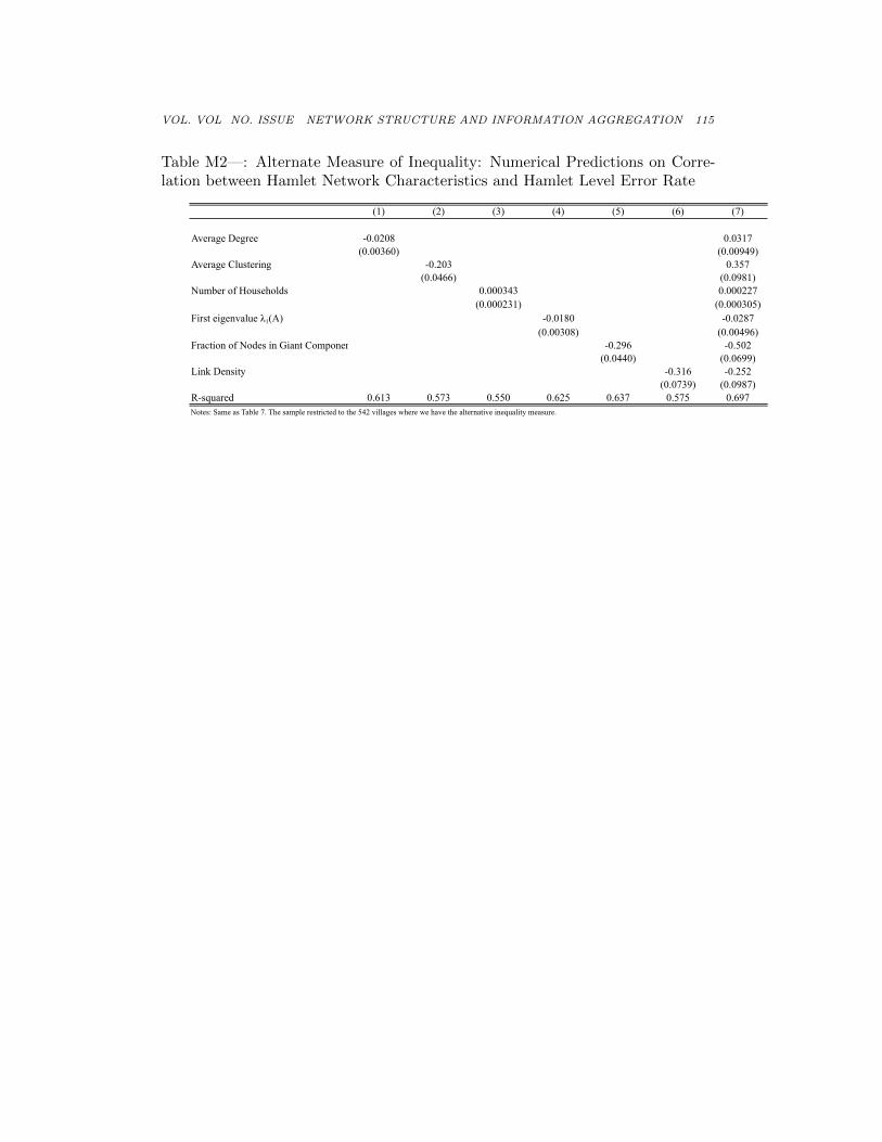
VOL. VOL NO. ISSUE NETWORK STRUCTURE AND INFORMATION AGGREGATION 115
Table M2—: Alternate Measure of Inequality: Numerical Predictions on Corre-lation between Hamlet Network Characteristics and Hamlet Level Error Rate
(1) (2) (3) (4) (5) (6) (7)
Average Degree -0.0208 0.0317(0.00360) (0.00949)
Average Clustering -0.203 0.357(0.0466) (0.0981)
Number of Households 0.000343 0.000227(0.000231) (0.000305)
First eigenvalue λ1(A) -0.0180 -0.0287(0.00308) (0.00496)
Fraction of Nodes in Giant Component -0.296 -0.502(0.0440) (0.0699)
Link Density -0.316 -0.252(0.0739) (0.0987)
R-squared 0.613 0.573 0.550 0.625 0.637 0.575 0.697Notes: Same as Table 7. The sample restricted to the 542 villages where we have the alternative inequality measure.

116 THE AMERICAN ECONOMIC REVIEW MONTH YEAR
Table M3—: Alternate Measure of Inequality: Empirical Results on StochasticDominance
(1) (2) (3) (4)
I fosd J -0.0935 -0.136 -0.0707 -0.0975(0.0193) (0.0298) (0.0199) (0.0303)
J fosd I 0.0465 0.0454(0.0184) (0.0196)
I fosd J -0.100 -0.170 -0.0715 -0.112(0.0177) (0.0264) (0.0194) (0.0288)
J fosd I 0.0730 0.0557(0.0168) (0.0188)
Non-Comparable Yes No Yes NoDemographic Controls No No Yes YesStratification Group FE Yes Yes Yes YesNotes: Same as Table 8. The sample restricted to the 542 villages where we have the alternative inequality measure.
Panel B: Self-Assessment Metric
Panel A: Consumption Metric
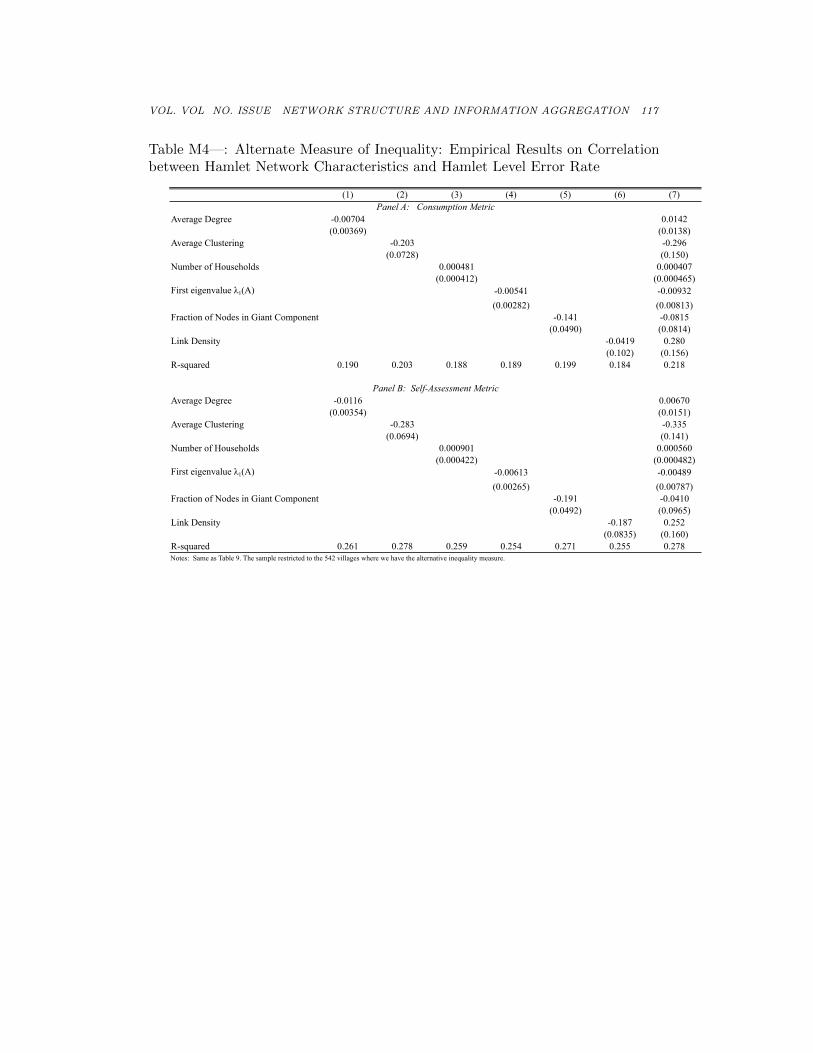
VOL. VOL NO. ISSUE NETWORK STRUCTURE AND INFORMATION AGGREGATION 117
Table M4—: Alternate Measure of Inequality: Empirical Results on Correlationbetween Hamlet Network Characteristics and Hamlet Level Error Rate
(1) (2) (3) (4) (5) (6) (7)
Average Degree -0.00704 0.0142(0.00369) (0.0138)
Average Clustering -0.203 -0.296(0.0728) (0.150)
Number of Households 0.000481 0.000407(0.000412) (0.000465)
First eigenvalue λ1(A) -0.00541 -0.00932(0.00282) (0.00813)
Fraction of Nodes in Giant Component -0.141 -0.0815(0.0490) (0.0814)
Link Density -0.0419 0.280(0.102) (0.156)
R-squared 0.190 0.203 0.188 0.189 0.199 0.184 0.218
Average Degree -0.0116 0.00670(0.00354) (0.0151)
Average Clustering -0.283 -0.335(0.0694) (0.141)
Number of Households 0.000901 0.000560(0.000422) (0.000482)
First eigenvalue λ1(A) -0.00613 -0.00489(0.00265) (0.00787)
Fraction of Nodes in Giant Component -0.191 -0.0410(0.0492) (0.0965)
Link Density -0.187 0.252(0.0835) (0.160)
R-squared 0.261 0.278 0.259 0.254 0.271 0.255 0.278Notes: Same as Table 9. The sample restricted to the 542 villages where we have the alternative inequality measure.
Panel A: Consumption Metric
Panel B: Self-Assessment Metric