Network Protocols

Chapters 13 and 15 (TCP/IP Suite Book):

TCP Congestion Control

Copyright © Lopamudra Roychoudhuri

1

Congestion Control

Congestion Load (number of packets sent) on the

network is greater than the capacity of the network

Congestion control refers to the mechanisms and

techniques to keep the load below the capacity

2

Congestion Control

We assumed that it is only the receiver that can dictate to the sender the size of the sender’s window.

We totally ignored another entity here, the network. In addition to the receiver, the network is a second entity that determines the size of the sender’s window.

3

Queue A queue consists of a number of packets.

These packets are bound to be routed over the network, lined up in a sequential way with a changing header and trailer and taken out of the queue for transmission by a network device.

If the router is unable to send a packet immediately, the packet is queued. If the queue is full, the packet is dropped.

Packets are typically processed on a first-come, first-served (or FIFO, First In First Out) basis. This adds up to best-effort forwarding.

4

Router queues

• Congestion occurs because routers and switches have queues and they forward all packets it receives to the best of its ability. It happens when:• Rate of packet arrival may be higher than packet

processing rate• Packet departure rate may be less than packet processing

rate

5

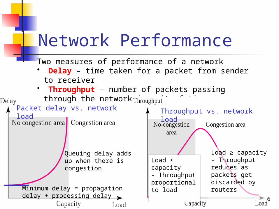
Packet delay vs. network load

Network PerformanceTwo measures of performance of a network• Delay – time taken for a packet from sender to

receiver• Throughput – number of packets passing through

the network in unit of time

Throughput vs. network load

Minimum delay = propagation delay + processing delay

Queuing delay adds up when there is congestion

Load < capacity- Throughput proportional to load

Load ≥ capacity- Throughput reduces as packets get discarded by routers

6

Congestion Window

We introduce new window called cwnd If the network cannot deliver the data

as fast as it is created by the sender, it must tell the sender to slow down

This is in addition to rwnd for flow control

Actual window size = min(cwnd, rwnd)

7

TCP Congestion Policy

TCP’s general policy for handling congestion is based on three phases: Slow Start Congestion avoidance Congestion detection

8

Slow start: Exponential Increase

Nothing slow about it! Size of cwnd starts with

one maximum segment size (MSS)- determined as a TCP option during connection establishment

After receiving each ACK, cwnd grows exponentially

- 1 -> 2 -> 4 -> 8 … Till it reaches slow start

threshold (ssthresh) In most implementations

the value of ssthresh is 65535 bytes

Assumption: rwnd > cwnd 9

Congestion Avoidance: Additive Increase

After reaching ssthresh, one must slow down the exponential growth

Size of the congestion window increases additively until congestion is detected

Increase by one: 1 -> 2 -> 3 -> 4 …

Assumption: rwnd > cwnd 10

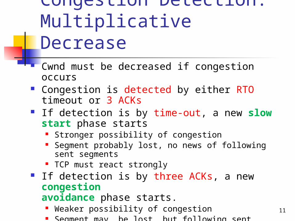
Congestion Detection: Multiplicative Decrease

Cwnd must be decreased if congestion occurs Congestion is detected by either RTO timeout or

3 ACKs If detection is by time-out, a new slow start

phase starts Stronger possibility of congestion Segment probably lost, no news of following sent

segments TCP must react strongly

If detection is by three ACKs, a new congestionavoidance phase starts.

Weaker possibility of congestion Segment may be lost, but following sent segments

might have reached TCP has a weaker reaction

11

TCP congestion policy summary

(Go back to Slow start)

(Do Congestion Avoidance)

12

Congestion example

13

at cwnd=20

ssthresh=20/2 = 10cwnd=1

at cwnd=12

ssthresh=12/2 = 6cwnd=ssthresh=6

Congestion example 2

14

A TCP sender starts sending segments. The initial ssthresh is set to 32 MSS. It receives 3 duplicate ACKs at cwnd =40. Later, there is an RTO timeout at 30.

a. Show the different phases (slow start, additive increase, multiplicative decrease), the ssthresh and the cwnd at various points.

b. Show the relevant calculations as well.

Congestion example 2

15

TCP Timer Management To perform its operation smoothly, most

TCP implementations use at least four timers: Retransmission timer (RTO) Persistence Keepalive TIME-WAIT

Retransmission timer (RTO): To retransmit lost segments, TCP employs one retransmission timer (for the whole connection period) that handles the retransmission time-out (RTO), the waiting time for an acknowledgment of a segment. 16

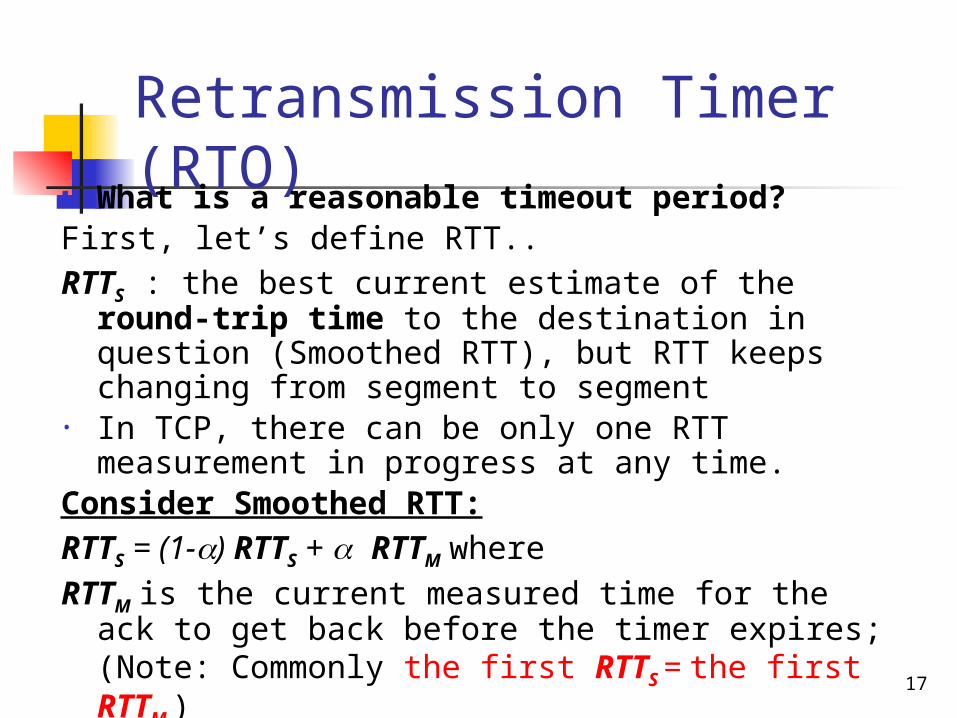
Retransmission Timer (RTO)

What is a reasonable timeout period?First, let’s define RTT..RTTS : the best current estimate of the round-trip

time to the destination in question (Smoothed RTT), but RTT keeps changing from segment to segment

• In TCP, there can be only one RTT measurement in progress at any time.

Consider Smoothed RTT:RTTS = (1-) RTTS + RTTM where RTTM is the current measured time for the ack to

get back before the timer expires; (Note: Commonly the first RTTS = the first RTTM )

is a smoothing factor that determines how much weight is given to the new value. Typically = 1/8

  

17

So, what is a reasonable timeout period?

Initial implementations, timeout = 2RTT -Inflexible and fails to respond when the variance

goes up Consider RTT Deviation:RTTD = (1-) RTTD + | RTTS - RTTM| where RTTD is an estimation of the standard

deviationand is a smoothing factor. Typically = 1/4 (Note: Commonly the first RTTD = ½ * the first RTTM )

And a ‘reasonable’ timeout period is..RTO = RTTS + 4* RTTD  

Retransmission Timer (RTO) cont.

18

Figure 15.39 Example 15.3 (hypothetical values)

(set initially)

19

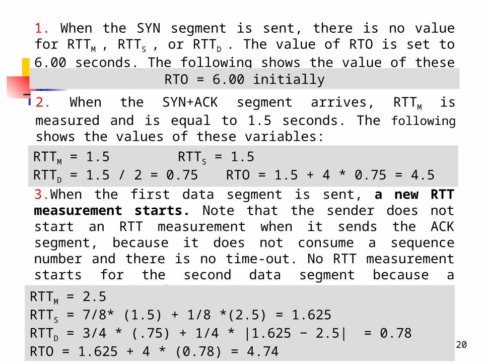
1. When the SYN segment is sent, there is no value for RTTM , RTTS , or RTTD . The value of RTO is set to 6.00 seconds. The following shows the value of these variables at this moment:

RTO = 6.00 initially

2. When the SYN+ACK segment arrives, RTTM is measured and is equal to 1.5 seconds. The following shows the values of these variables:

RTTM = 1.5 RTTS = 1.5RTTD = 1.5 / 2 = 0.75 RTO = 1.5 + 4 * 0.75 = 4.53.When the first data segment is sent, a new RTT measurement starts. Note that the sender does not start an RTT measurement when it sends the ACK segment, because it does not consume a sequence number and there is no time-out. No RTT measurement starts for the second data segment because a measurement is already in progress.

RTTM = 2.5RTTS = 7/8* (1.5) + 1/8 *(2.5) = 1.625RTTD = 3/4 * (.75) + 1/4 * |1.625 − 2.5| = 0.78RTO = 1.625 + 4 * (0.78) = 4.74 20

Suppose that a segment is not acknowledged during the retransmission timeout period and is therefore retransmitted.

When the sending TCP receives an acknowledgment for this segment, it does not know if the acknowledgment is for the original segment or for the retransmitted one.

The value of RTT is based on the departure of segment which one to consider, original or retransmitted?

Karn’s Algorithm Do not consider the RTT of a retransmitted

segment in the calculation of a new RTT Do not update the value of RTT until you send a

segment and receive an acknowledgement without the need for retransmission

Karn's algorithm

21

Exponential Backoff

What is the value of RTO if retransmission occurs?

Most TCP implementations use an exponential backoff strategy.

Value of RTO is doubled for each retransmission If the segment is retransmitted once, the value

is two times the RTO. If it transmitted twice, the value is four times

the RTO, and so on.22

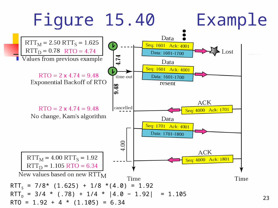
Figure 15.40 Example 15.4

RTTS = 7/8* (1.625) + 1/8 *(4.0) = 1.92RTTD = 3/4 * (.78) + 1/4 * |4.0 − 1.92| = 1.105RTO = 1.92 + 4 * (1.105) = 6.34

23

Figure 15.40 is a continuation of the previous example. There is retransmission and Karn’s algorithm is applied. The first segment in the figure is sent, but lost. The RTO timer expires after 4.74 seconds. The segment is retransmitted and the timer is set to 9.48, twice the previous value of RTO. This time an ACK is received before the time-out. We wait until we send a new segment and receive the ACK for it before recalculating the RTO (Karn’s algorithm).

Example 15.4 cont.

24

TCP Timer Management (Read yourself pgs 481- 482) Persistence Timer

To deal with a zero-window-size advertisement, TCP needs another timer.

If the receiving TCP announces a window size of zero, the sending TCP stops transmitting segments until the receiving TCP sends an ACK segment announcing a nonzero window size.

This ACK segment can be lost. Remember that ACK segments are not acknowledged nor retransmitted in TCP.

25

TCP Timer Management (Read yourself pgs 481- 482) Persistence Timer If this acknowledgment is lost, the receiving

TCP thinks that it has done its job and waits for the sending TCP to send more segments.

Both TCPs might continue to wait for each other forever (a deadlock). To correct this deadlock, TCP uses a persistence timer for each connection.

26

TCP Timer Management (Read yourself pgs 481- 482) Keepalive Timer

When a connection has been idle, check to see if the other side is still there.

Example: A client opens a TCP connection to a server, transfers some data, and becomes silent. Perhaps the client has crashed. In this case, the connection remains open forever.

To remedy this situation, most implementations equip a server with a keepalive timer. Each time the server hears from a client, it resets this timer.

27

TCP Timer Management (Read yourself pgs 481- 482) Keepalive Timer

The time-out is usually 2 hours. If the server does not hear from the client after 2 hours, it sends a probe segment.

If there is no response after 10 probes, each of which is 75 s apart, it assumes that the client is down and terminates the connection.

28

TCP Timer Management (Read yourself pgs 481- 482)

Time-Waited Timer (2MSL) During connection termination. A connection is

not considered really closed until the end of a time-waited period. Usually two times the expected lifetime of a segment

29

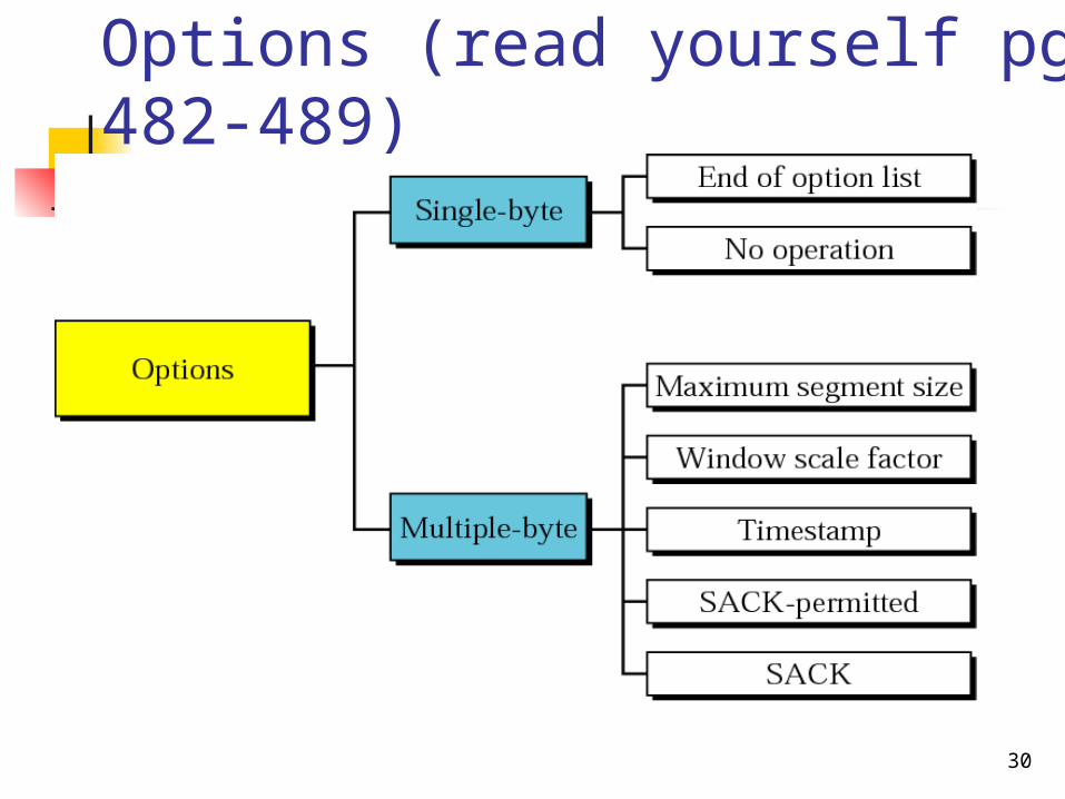
Options (read yourself pgs 482-489)

30

Maximum Segment Size (MSS)

The maximum-segment-size option defines the size of the biggest unit of data that can be received by the destination of the TCP segment.

In spite of its name, it defines the maximum size of the data, not the maximum size of the segment.

Since the field is 16 bits long, the value can be 0 to 65,535 bytes.

31

Maximum Segment Size (MSS) MSS is determined during connection

establishment and does not change during the connection. Each party defines the MSS or the segments it will receive during the connection.

If a party does not define this, the default values is 536 bytes.

32

Window Scale Factor

The window size field in the header defines the size of the sliding window. The window can be up to 65535 bytes.

To increase the window size, a window scale factor is used.

The value of the window scale factor can be determined only during connection establishment; it does not change during the connection.

33

Window Scale Factor

During data transfer, the size of the window (specified in the header) may be changed, but it must be multiplied by the same window scale factor

Note that one end may set the value of the window scale factor to 0, which means that although it supports this option, but it does not want to use it for this connection.

34

Window Scale Factor Example For example, suppose the value of the window

scale factor is 3. An end point receives an acknowledgment in which the window size is advertised as 32,768. Solution: The size of window this end can use is 32,768 × 2^3 = 262,144 bytes.

Although the scale factor could be as large as 255, the largest value allowed by TCP/IP is 14, which means that the maximum window size is 2^16 × 2^ 14 = 2^30, which is less than the maximum value for the sequence number.

Note that the size of the window cannot be greater than the maximum value of the sequence number.

35

Window Scale Factor Another Example

For example, suppose the value of the window scale factor is 8. An end point receives an acknowledgment in which the window size is advertised as 8192.

Solution: The size of window this end can use is 8192 × 2^8 or 2,097,152 bytes.

36

Timestamp

The timestamp option has two applications: it measures the round-trip time and prevents wraparound sequence numbers.

TCP, when ready to send a segment, reads the value of the system clock and inserts this value, a 32-bit number, in the timestamp value field.

Note that there is no need for the sender’s and receiver’s clocks to be synchronized because all calculations are based on the sender clock.

Example 15.5: This is actually the meaning of RTT: the time difference between a packet sent and the acknowledgment received.

37

Figure 15.47 Example 15.5

RTT: the time difference between a packet sent and the acknowledgment received.

38

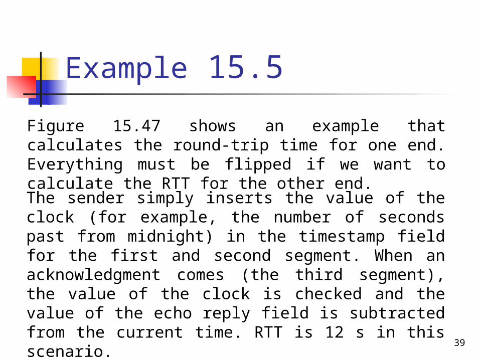
Figure 15.47 shows an example that calculates the round-trip time for one end. Everything must be flipped if we want to calculate the RTT for the other end.

Example 15.5

The sender simply inserts the value of the clock (for example, the number of seconds past from midnight) in the timestamp field for the first and second segment. When an acknowledgment comes (the third segment), the value of the clock is checked and the value of the echo reply field is subtracted from the current time. RTT is 12 s in this scenario.

39

SACK

If some segments are lost or dropped, the sender must wait until a time-out and then send all segments that have not been acknowledged. The receiver may receive duplicate segments.

The Selective Acknowledgment (SACK) allows the sender to have a better idea of which segments are actually lost and which have arrived out of order.

The new proposal even includes a list for

duplicate segments. The sender can then send only those segments that are really lost.

40

SACK

The list of duplicate segments can help the sender find the segments which have been retransmitted by a short time-out.

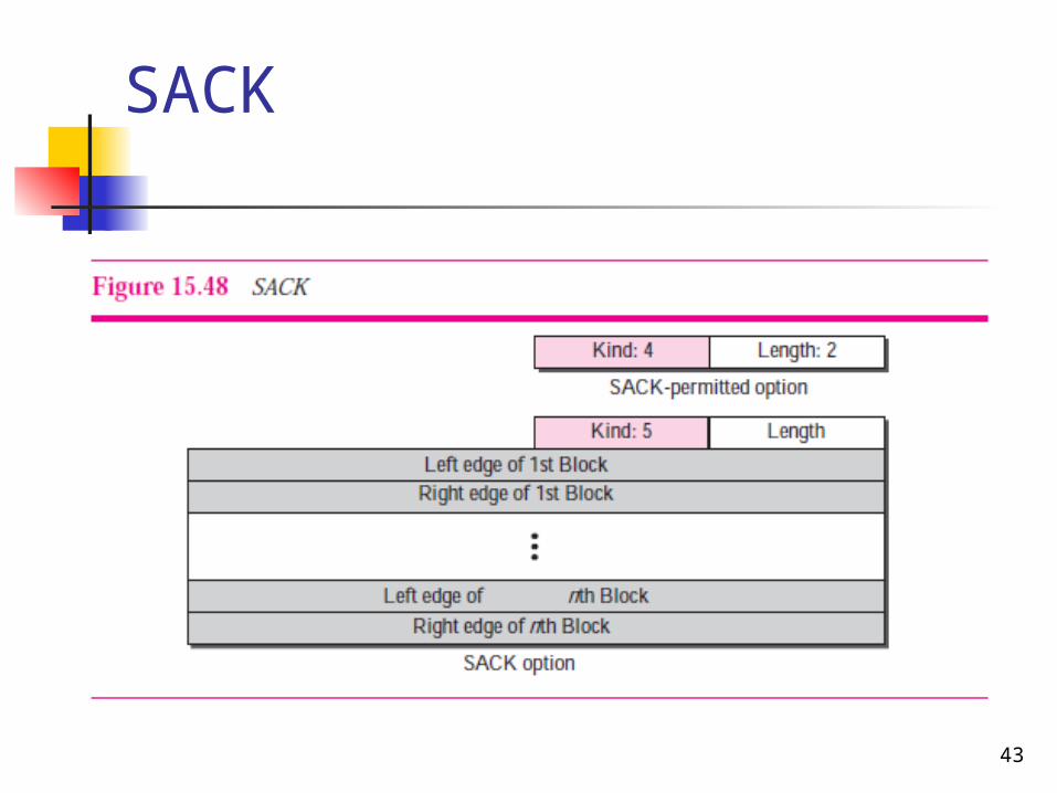
The SACK-permitted option of two bytes is used only during connection establishment. The host that sends the SYN segment adds this option to show that it can support the SACK option. If the other end, in its SYN + ACK segment, also includes this option, then the two ends can use the SACK option during data transfer.

41

SACK

Note that the SACK-permitted option is not allowed during the data transfer phase.

SACK option, is used during data transfer only if both ends agree (if they have exchanged SACK-permitted options during connection establishment).

The option includes a list for blocks arriving out of order. Each block occupies two 32-bit numbers that define the beginning and the end of the blocks.

Remember that the allowed size of an option in TCP is only 40 bytes

42

43

SACK

44

SACK Example

45

SACK Another Example

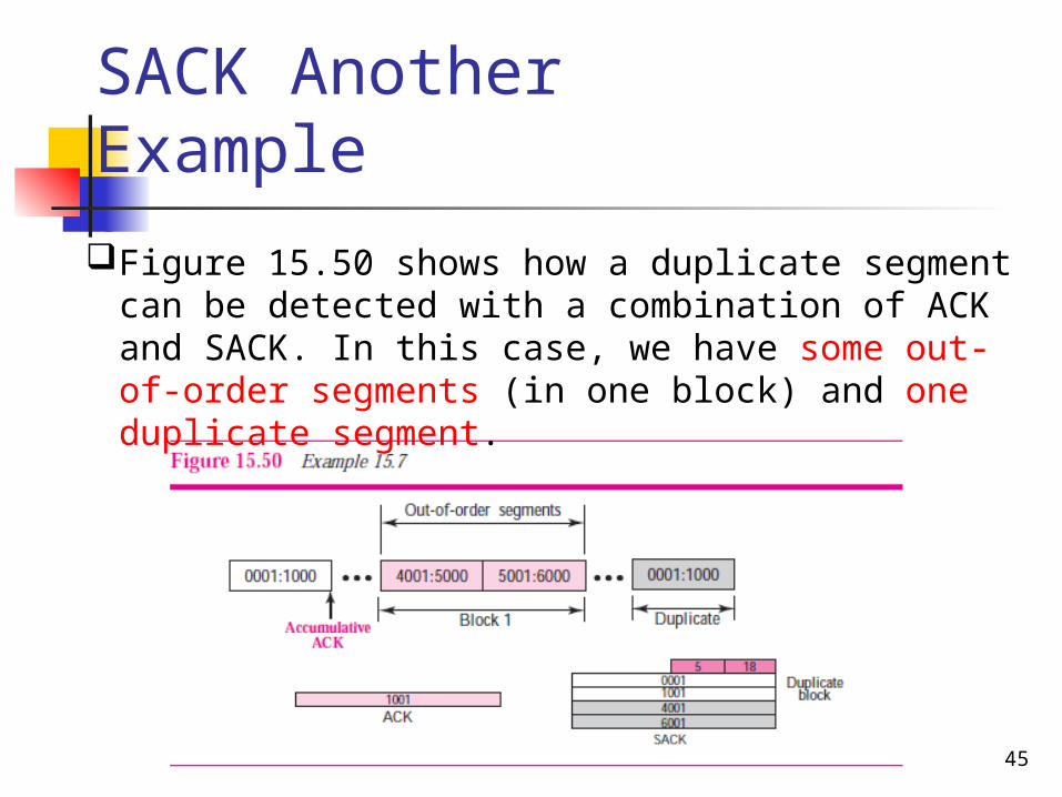
Figure 15.50 shows how a duplicate segment can be detected with a combination of ACK and SACK. In this case, we have some out-of-order segments (in one block) and one duplicate segment.