Embed Size (px)
Citation preview
Network LayerRouting in Packet Networks
Shortest Path Routing
Topic 6: Routing (Network Layer)
ReferenceA. Leon-Garcia and I. Widjaja, Communication Networks, pp. 492-495, 515-520, 522-534.
(Reserved in the DC library. Call No. TK5105. L46 2004.)
Network Layer Overview
Network Layer Services
Network Layer Functions
6.1 Network Layer
3
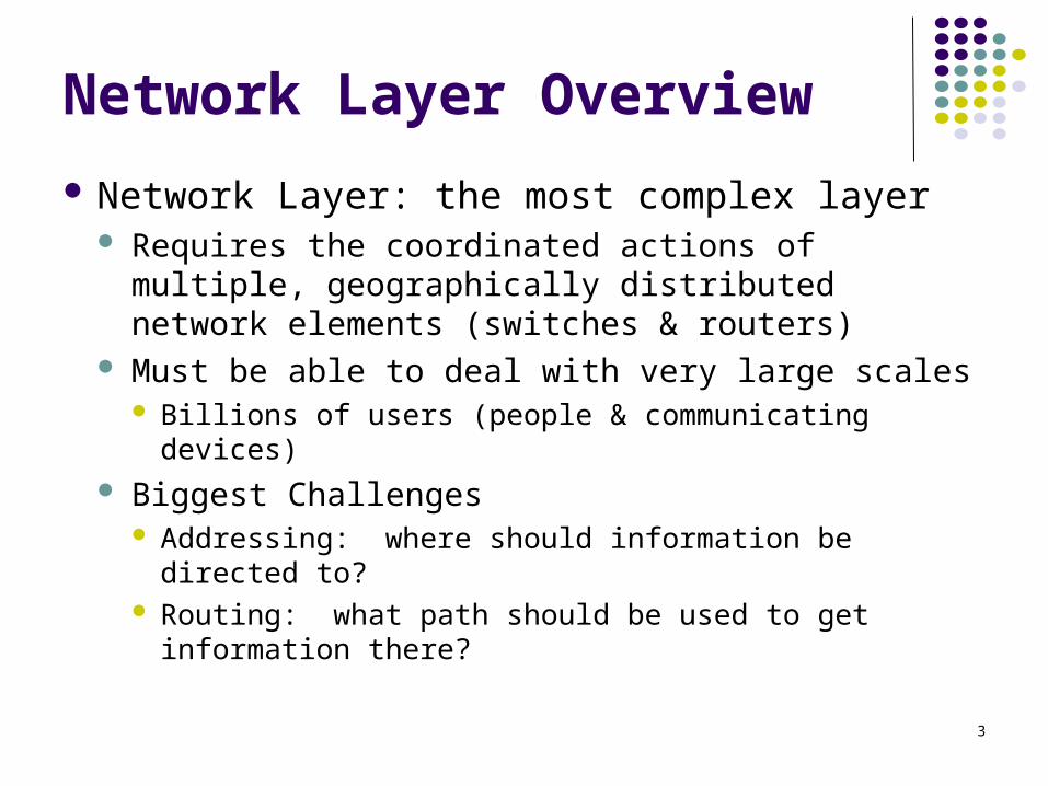
Network Layer Overview
Network Layer: the most complex layer Requires the coordinated actions of multiple,
geographically distributed network elements (switches & routers)
Must be able to deal with very large scales Billions of users (people & communicating devices)
Biggest Challenges Addressing: where should information be directed to? Routing: what path should be used to get information
there?
4
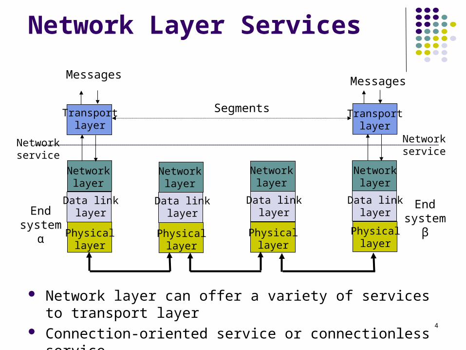
End system
βPhysicallayer
Data linklayer
Physicallayer
Data linklayerEnd
systemα
Networklayer
Networklayer
Physicallayer
Data linklayer
Networklayer
Physicallayer
Data linklayer
Networklayer
Transportlayer
Transportlayer
MessagesMessages
Segments
Networkservice
Networkservice
Network layer can offer a variety of services to transport layer Connection-oriented service or connectionless service Best-effort or delay/loss guarantees
Network Layer Services
5
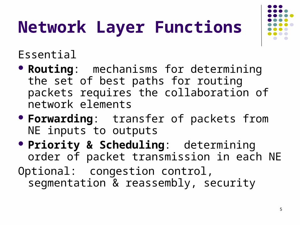
Network Layer Functions
Essential Routing: mechanisms for determining the
set of best paths for routing packets requires the collaboration of network elements
Forwarding: transfer of packets from NE inputs to outputs
Priority & Scheduling: determining order of packet transmission in each NE
Optional: congestion control, segmentation & reassembly, security
Packet Networks
Routing Tables
Routing Algorithms
IP Addressing
6.2 Routing in Packet Networks
7
1
2
3
4
5
6
Node (switch or router)
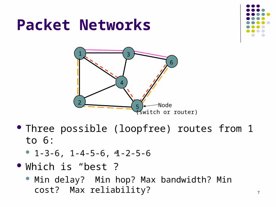
Packet Networks
Three possible (loopfree) routes from 1 to 6: 1-3-6, 1-4-5-6, 1-2-5-6
Which is “best”? Min delay? Min hop? Max bandwidth? Min cost?
Max reliability?
8
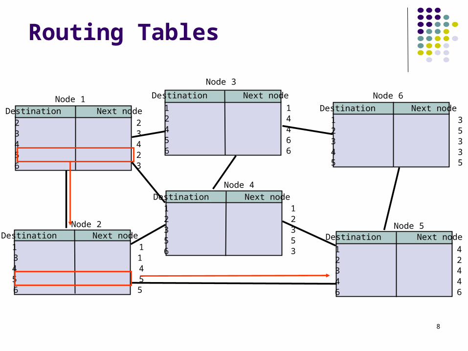
2 2 3 3 4 4 5 2 6 3
Node 1
Node 2
Node 3
Node 4
Node 6
Node 5
1 1 2 4 4 4 5 6 6 6
1 3 2 5 3 3 4 3 5 5
Destination Next node 1 1 3 1 4 4 5 5 6 5
1 4 2 2 3 4 4 4 6 6
1 1 2 2 3 3 5 5 6 3
Destination Next node
Destination Next node
Destination Next node
Destination Next node
Destination Next node
Routing Tables
9
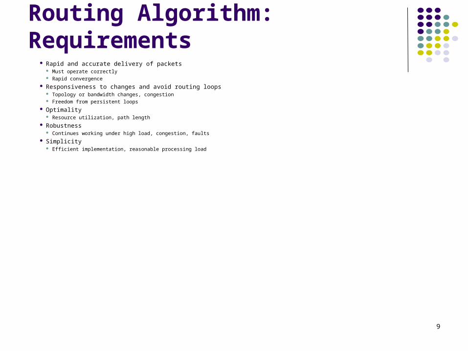
Routing Algorithm: Requirements Rapid and accurate delivery of packets
Must operate correctly Rapid convergence
Responsiveness to changes and avoid routing loops Topology or bandwidth changes, congestion Freedom from persistent loops
Optimality Resource utilization, path length
Robustness Continues working under high load, congestion, faults
Simplicity Efficient implementation, reasonable processing load
10
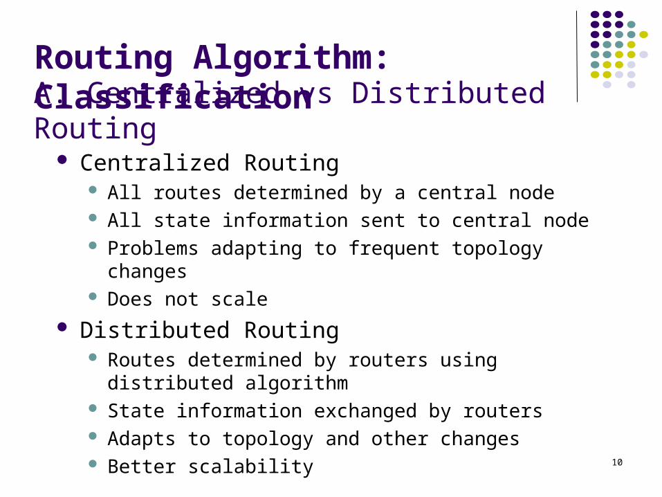
A. Centralized vs Distributed Routing Centralized Routing
All routes determined by a central node All state information sent to central node Problems adapting to frequent topology changes Does not scale
Distributed Routing Routes determined by routers using distributed
algorithm State information exchanged by routers Adapts to topology and other changes Better scalability
Routing Algorithm: Classification
11
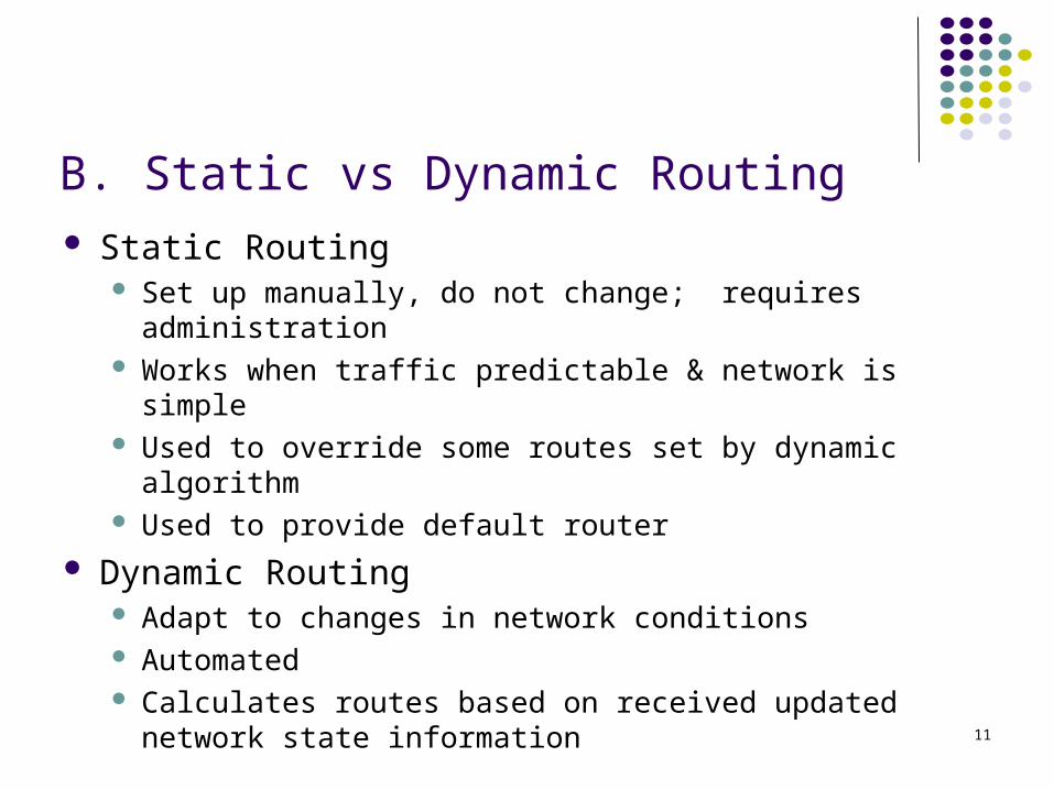
B. Static vs Dynamic Routing Static Routing
Set up manually, do not change; requires administration Works when traffic predictable & network is simple Used to override some routes set by dynamic algorithm Used to provide default router
Dynamic Routing Adapt to changes in network conditions Automated Calculates routes based on received updated network
state information
12
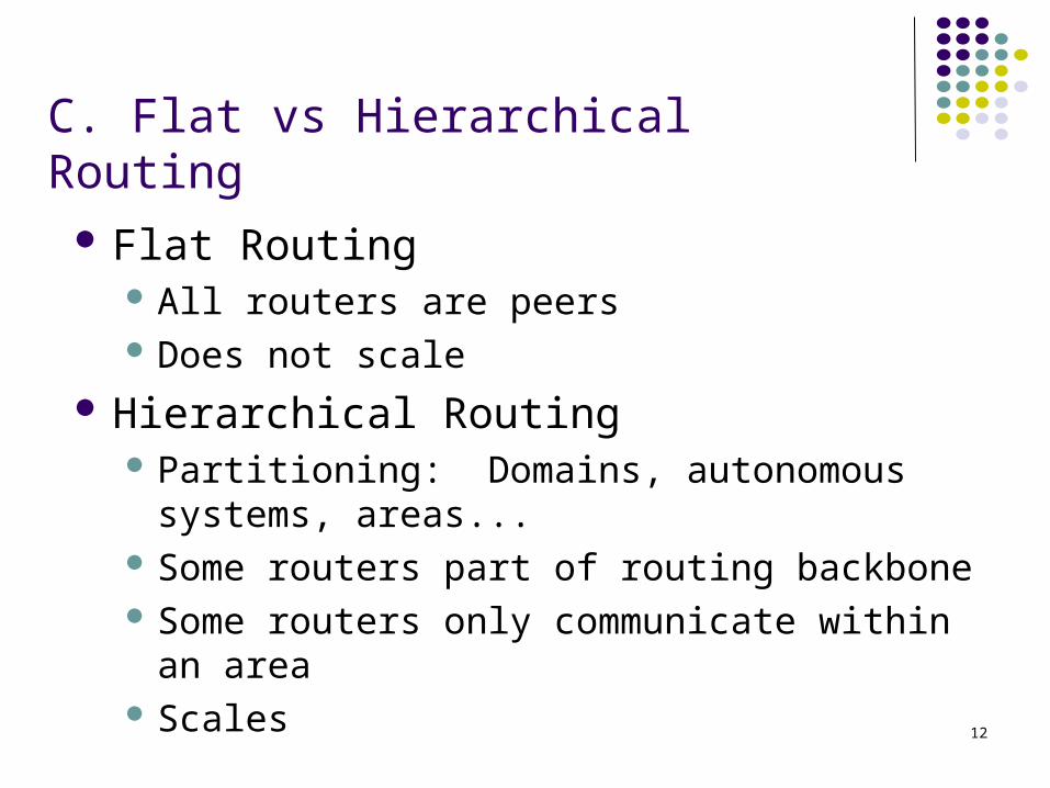
C. Flat vs Hierarchical Routing Flat Routing
All routers are peers Does not scale
Hierarchical Routing Partitioning: Domains, autonomous systems,
areas... Some routers part of routing backbone Some routers only communicate within an area Scales
13
0000 0111 1010 1101
0001 0100 1011 1110
0011 0101 1000 1111
0011 0110 1001 1100
R1
1
2 5
4
3
0000 1 0111 1 1010 1 … …
0001 4 0100 4 1011 4 … …
R2
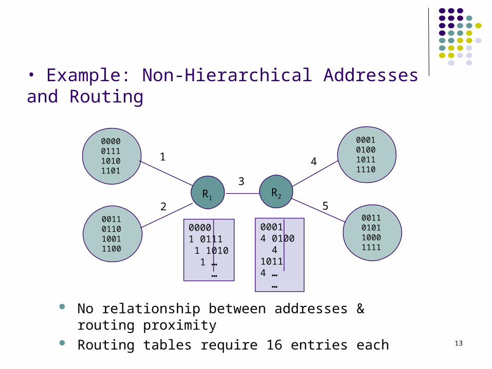
• Example: Non-Hierarchical Addresses and Routing
No relationship between addresses & routing proximity Routing tables require 16 entries each
14
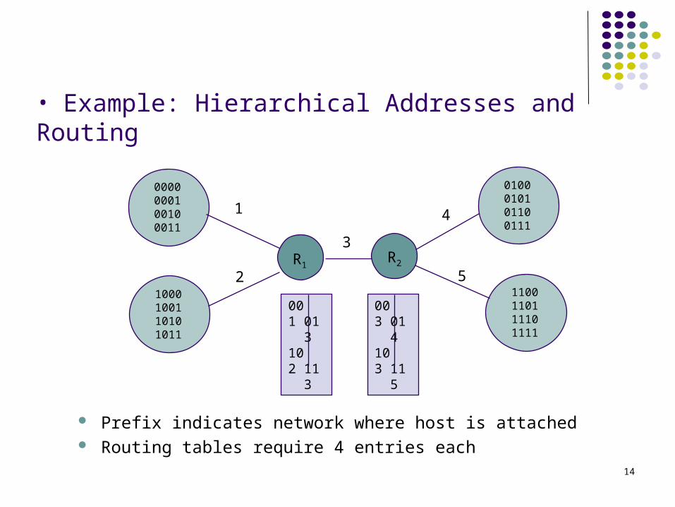
• Example: Hierarchical Addresses and Routing
Prefix indicates network where host is attached Routing tables require 4 entries each
0000 0001 0010 0011
0100 0101 0110 0111
1100 1101 1110 1111
1000 1001 1010 1011
R1R2
1
2 5
4
3
00 1 01 3 10 2 11 3
00 3 01 4 10 3 11 5
IP Addressing
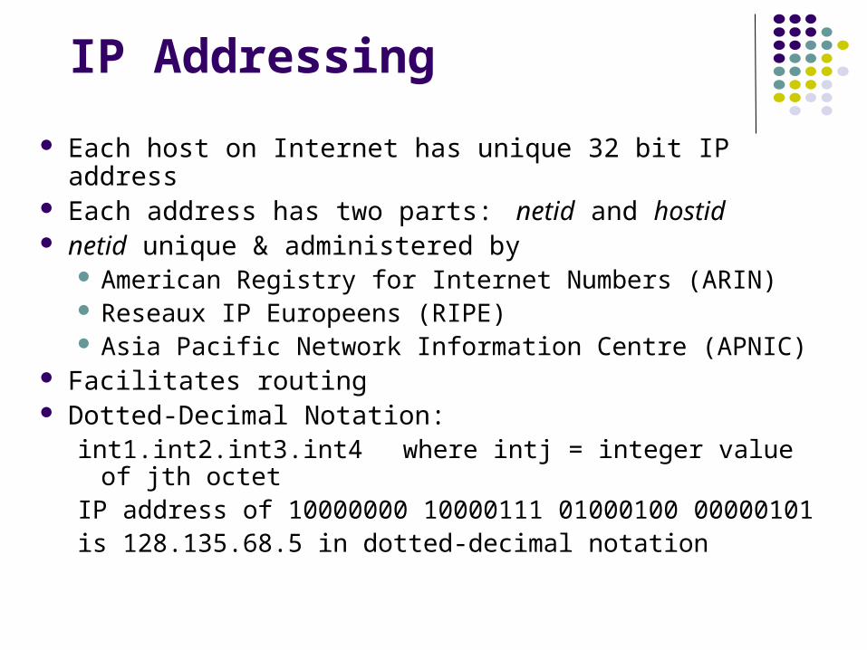
Each host on Internet has unique 32 bit IP address Each address has two parts: netid and hostid netid unique & administered by
American Registry for Internet Numbers (ARIN) Reseaux IP Europeens (RIPE) Asia Pacific Network Information Centre (APNIC)
Facilitates routing Dotted-Decimal Notation:
int1.int2.int3.int4 where intj = integer value of jth octetIP address of 10000000 10000111 01000100 00000101is 128.135.68.5 in dotted-decimal notation
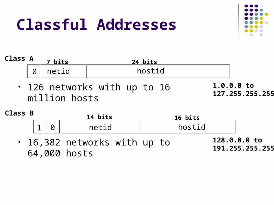
Classful Addresses
0
1 0
netid
netid
hostid
hostid
7 bits 24 bits
14 bits 16 bits
Class A
Class B
• 126 networks with up to 16 million hosts
• 16,382 networks with up to 64,000 hosts
1.0.0.0 to127.255.255.255
128.0.0.0 to191.255.255.255
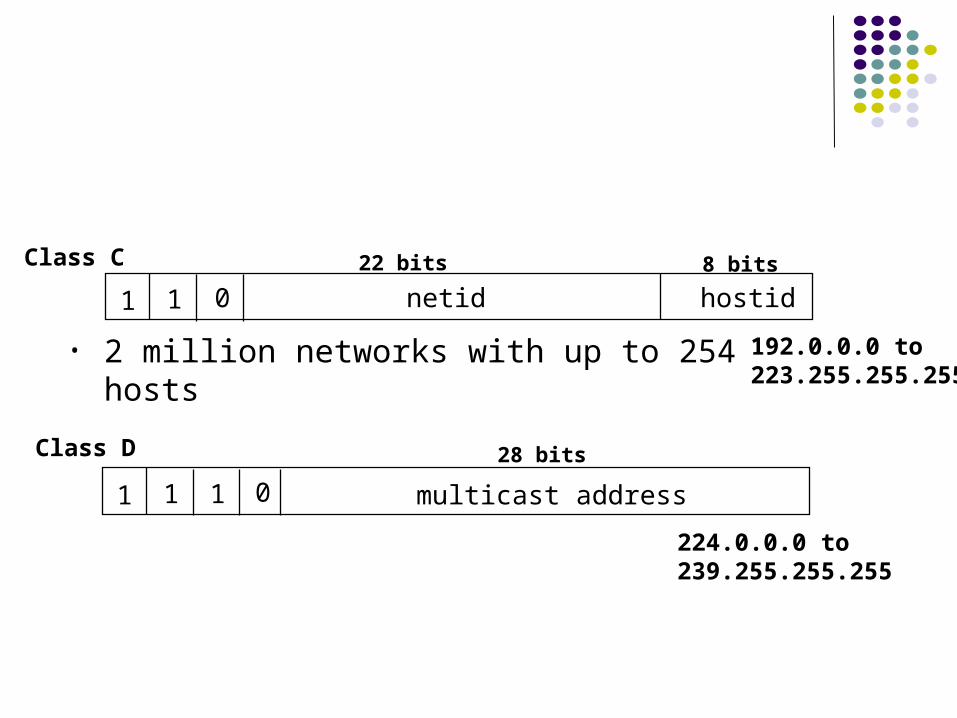
1 1 multicast address
28 bits
1 0
Class D
224.0.0.0 to239.255.255.255
1 1 netid hostid22 bits 8 bitsClass C
0
• 2 million networks with up to 254 hosts 192.0.0.0 to223.255.255.255
Private IP Addresses
Specific ranges of IP addresses set aside for use in private networks (RFC 1918)
Use restricted to private internets; routers in public Internet discard packets with these addresses
Range 1: 10.0.0.0 to 10.255.255.255 Range 2: 172.16.0.0 to 172.31.255.255 Range 3: 192.168.0.0 to 192.168.255.255 Network Address Translation (NAT) used to
convert between private & global IP addresses
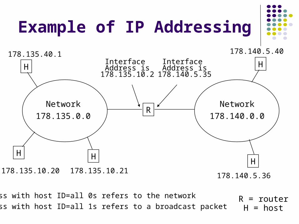
Example of IP Addressing
RNetwork
178.135.0.0
Network
178.140.0.0
H H
HH H
R = routerH = host
Interface Address is
178.135.10.2
Interface Address is
178.140.5.35
178.135.10.20 178.135.10.21
178.135.40.1
178.140.5.36
178.140.5.40
Address with host ID=all 0s refers to the network
Address with host ID=all 1s refers to a broadcast packet
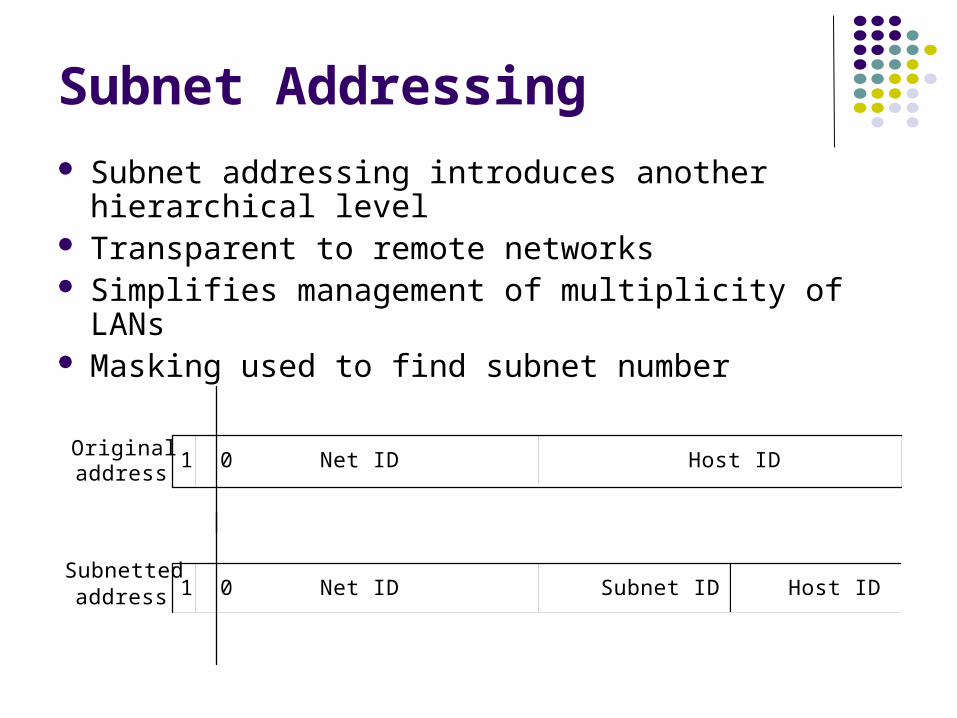
Subnet Addressing
Subnet addressing introduces another hierarchical level
Transparent to remote networks Simplifies management of multiplicity of LANs Masking used to find subnet number
Originaladdress
Subnettedaddress
Net ID Host ID1 0
Net ID Host ID1 0 Subnet ID
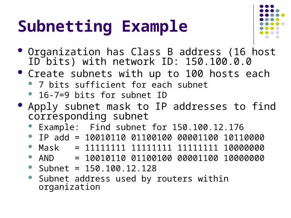
Subnetting Example Organization has Class B address (16 host ID bits)
with network ID: 150.100.0.0 Create subnets with up to 100 hosts each
7 bits sufficient for each subnet 16-7=9 bits for subnet ID
Apply subnet mask to IP addresses to find corresponding subnet Example: Find subnet for 150.100.12.176 IP add = 10010110 01100100 00001100 10110000 Mask = 11111111 11111111 11111111 10000000 AND = 10010110 01100100 00001100 10000000 Subnet = 150.100.12.128 Subnet address used by routers within organization
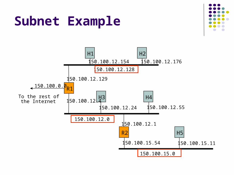
R1
H1 H2
H3 H4
R2 H5
To the rest ofthe Internet
150.100.0.0
150.100.12.128
150.100.12.0
150.100.12.176150.100.12.154
150.100.12.24 150.100.12.55
150.100.12.1
150.100.15.54
150.100.15.0
150.100.15.11
150.100.12.129
150.100.12.4
Subnet Example
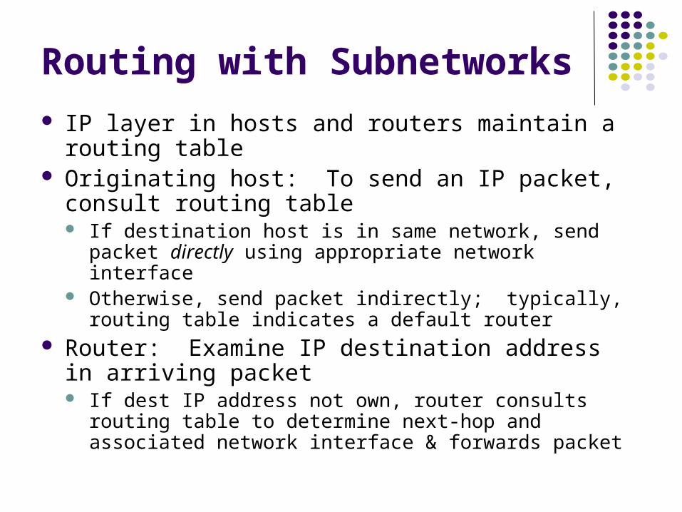
Routing with Subnetworks
IP layer in hosts and routers maintain a routing table Originating host: To send an IP packet, consult
routing table If destination host is in same network, send packet directly
using appropriate network interface Otherwise, send packet indirectly; typically, routing table
indicates a default router Router: Examine IP destination address in arriving
packet If dest IP address not own, router consults routing table to
determine next-hop and associated network interface & forwards packet
Shortest Path Problem
Routing Metrics
Shortest Path Protocols
6.3 Shortest Path Routing
25
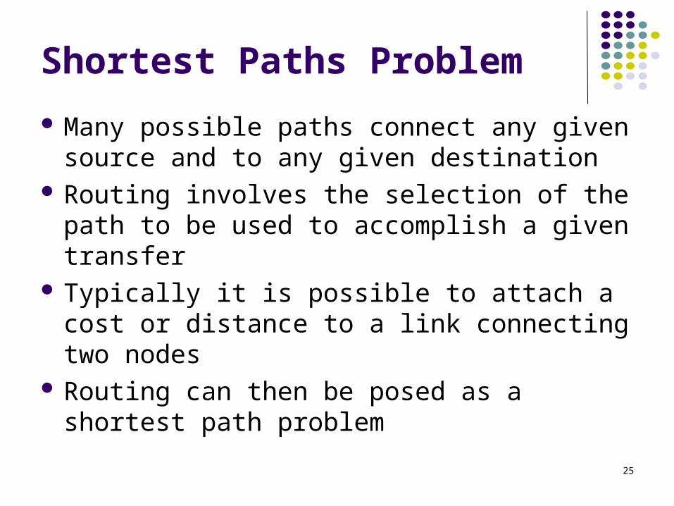
Shortest Paths Problem
Many possible paths connect any given source and to any given destination
Routing involves the selection of the path to be used to accomplish a given transfer
Typically it is possible to attach a cost or distance to a link connecting two nodes
Routing can then be posed as a shortest path problem
26
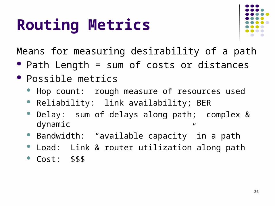
Routing Metrics
Means for measuring desirability of a path Path Length = sum of costs or distances Possible metrics
Hop count: rough measure of resources used Reliability: link availability; BER Delay: sum of delays along path; complex & dynamic Bandwidth: “available capacity” in a path Load: Link & router utilization along path Cost: $$$
27
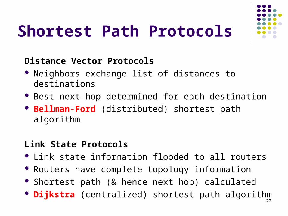
Shortest Path Protocols
Distance Vector Protocols Neighbors exchange list of distances to destinations Best next-hop determined for each destination Bellman-Ford (distributed) shortest path algorithm
Link State Protocols Link state information flooded to all routers Routers have complete topology information Shortest path (& hence next hop) calculated Dijkstra (centralized) shortest path algorithm
28
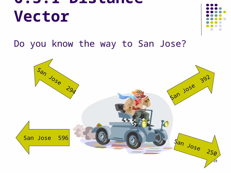
San Jose 392
San Jose 596
San Jose 294
San Jose 250
6.3.1 Distance Vector
Do you know the way to San Jose?
29
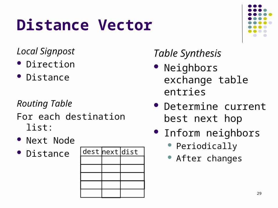
Distance Vector
Local Signpost Direction Distance
Routing Table
For each destination list: Next Node Distance
Table Synthesis Neighbors exchange
table entries Determine current best
next hop Inform neighbors
Periodically After changes
dest next dist
30
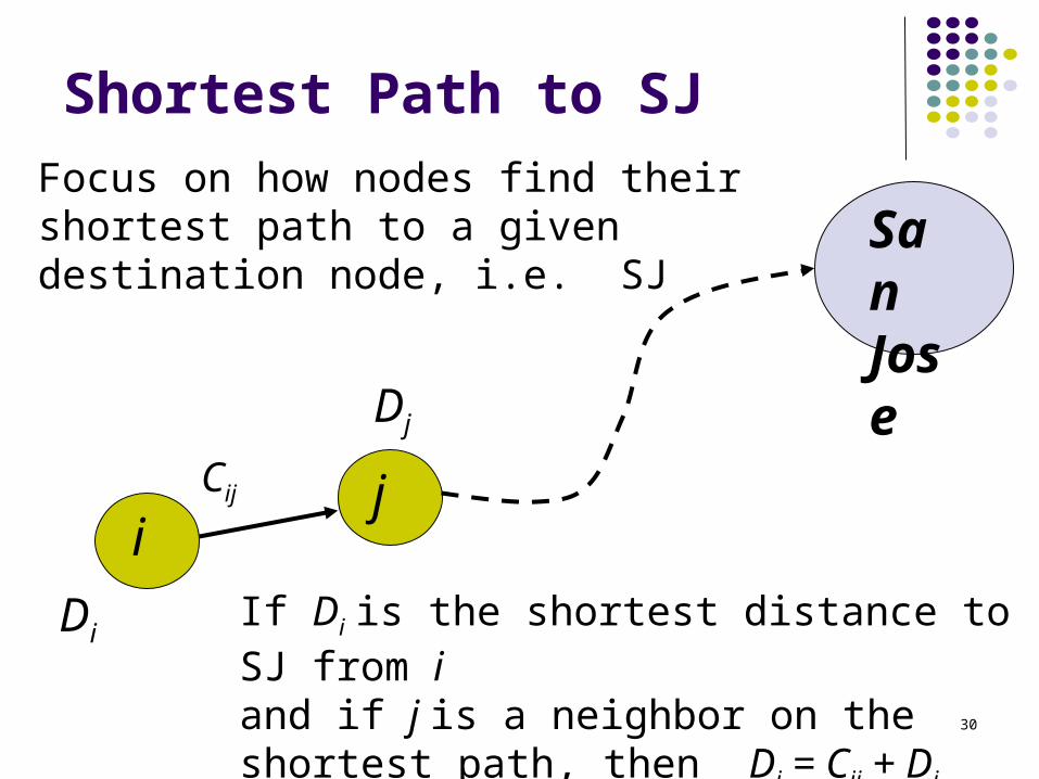
Shortest Path to SJ
ij
SanJose
Cij
Dj
DiIf Di is the shortest distance to SJ from iand if j is a neighbor on the shortest path, then Di = Cij + Dj
Focus on how nodes find their shortest path to a given destination node, i.e. SJ
31
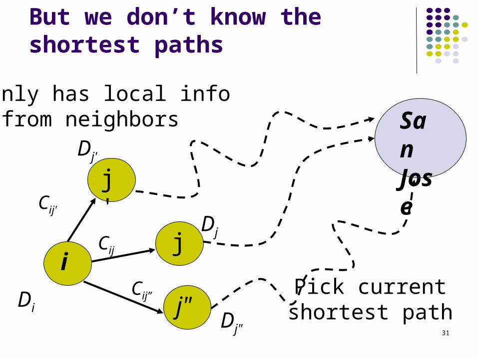
i only has local infofrom neighbors
Dj"
Cij”
i
SanJose
jCij
Dj
Di j"
Cij'
j'Dj'
Pick current shortest path
But we don’t know the shortest paths
32
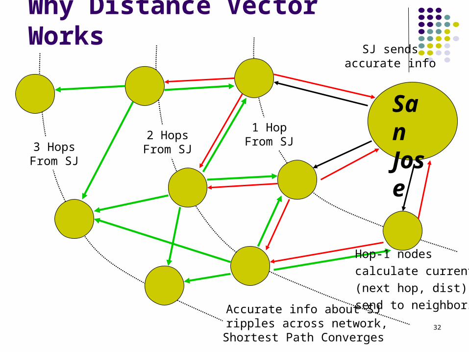
Why Distance Vector Works
SanJose
1 HopFrom SJ2 Hops
From SJ3 HopsFrom SJ
Accurate info about SJ ripples across network,
Shortest Path Converges
SJ sendsaccurate info
Hop-1 nodes
calculate current
(next hop, dist), &
send to neighbors
33
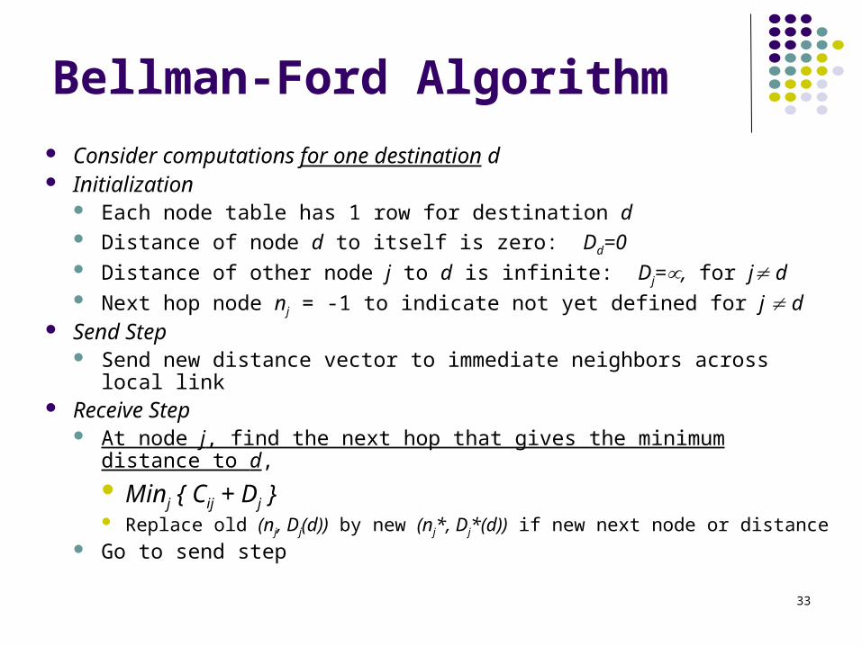
Bellman-Ford Algorithm
Consider computations for one destination d Initialization
Each node table has 1 row for destination d Distance of node d to itself is zero: Dd=0 Distance of other node j to d is infinite: Dj=, for j d Next hop node nj = -1 to indicate not yet defined for j d
Send Step Send new distance vector to immediate neighbors across local link
Receive Step At node j, find the next hop that gives the minimum distance to d,
Minj { Cij + Dj } Replace old (nj, Dj(d)) by new (nj*, Dj*(d)) if new next node or distance
Go to send step
34
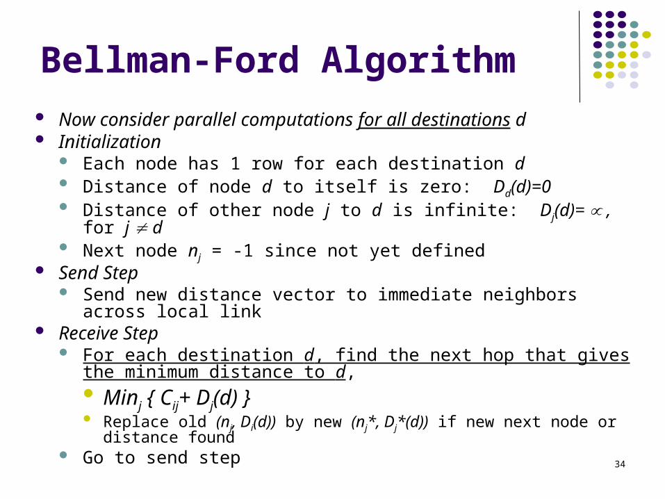
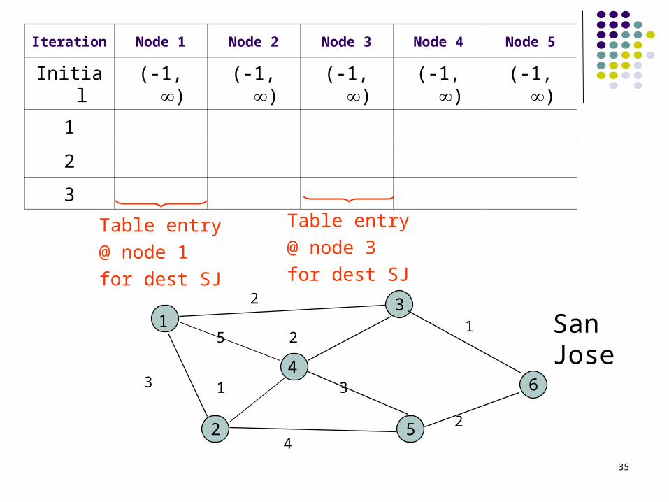
Bellman-Ford Algorithm Now consider parallel computations for all destinations d Initialization
Each node has 1 row for each destination d Distance of node d to itself is zero: Dd(d)=0 Distance of other node j to d is infinite: Dj(d)= , for j d Next node nj = -1 since not yet defined
Send Step Send new distance vector to immediate neighbors across local link
Receive Step For each destination d, find the next hop that gives the minimum
distance to d, Minj { Cij+ Dj(d) } Replace old (nj, Di(d)) by new (nj*, Dj*(d)) if new next node or distance
found Go to send step
35
Iteration Node 1 Node 2 Node 3 Node 4 Node 5
Initial (-1, ) (-1, ) (-1, ) (-1, ) (-1, )
1
2
3
31
5
46
2
2
3
4
2
1
1
2
3
5SanJose
Table entry
@ node 1
for dest SJ
Table entry
@ node 3
for dest SJ
36
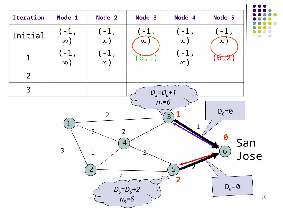
Iteration Node 1 Node 2 Node 3 Node 4 Node 5
Initial (-1, ) (-1, ) (-1, ) (-1, ) (-1, )
1 (-1, ) (-1, ) (6,1) (-1, ) (6,2)
2
3
SanJose
D6=0
D3=D6+1n3=6
31
5
46
2
2
3
4
2
1
1
2
3
5
D6=0D5=D6+2n5=6
0
2
1
37
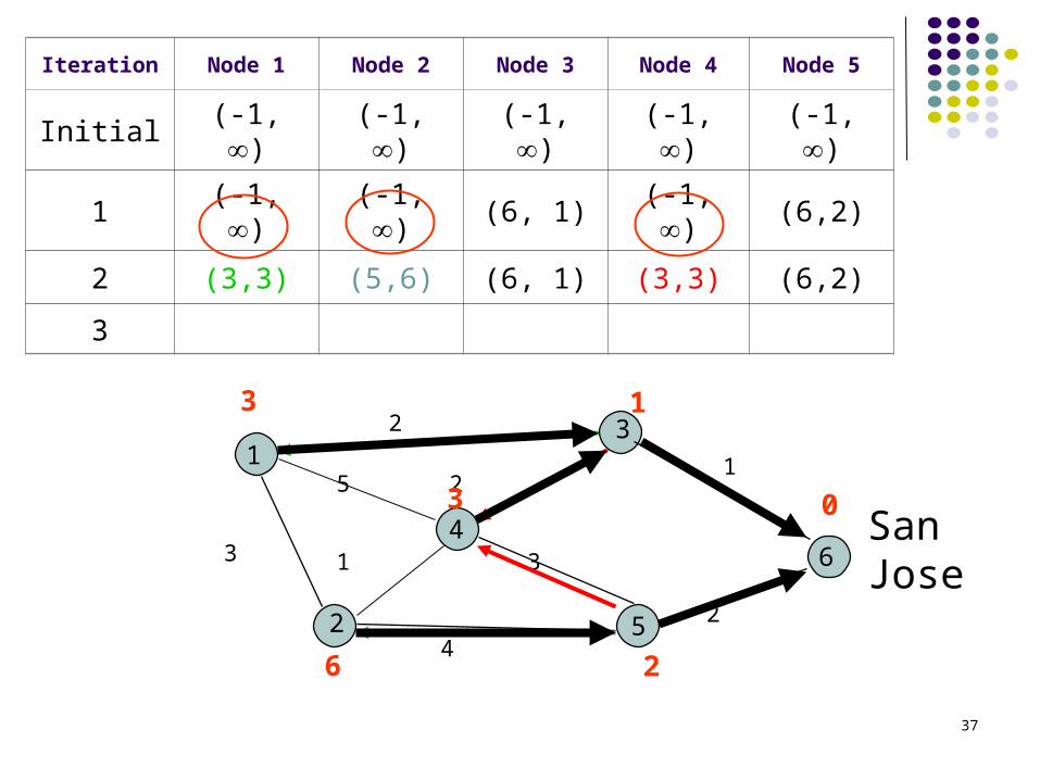
Iteration Node 1 Node 2 Node 3 Node 4 Node 5
Initial (-1, ) (-1, ) (-1, ) (-1, ) (-1, )
1 (-1, ) (-1, ) (6, 1) (-1, ) (6,2)
2 (3,3) (5,6) (6, 1) (3,3) (6,2)
3
SanJose
31
5
46
2
2
3
4
2
1
1
2
3
50
1
2
3
3
6
38
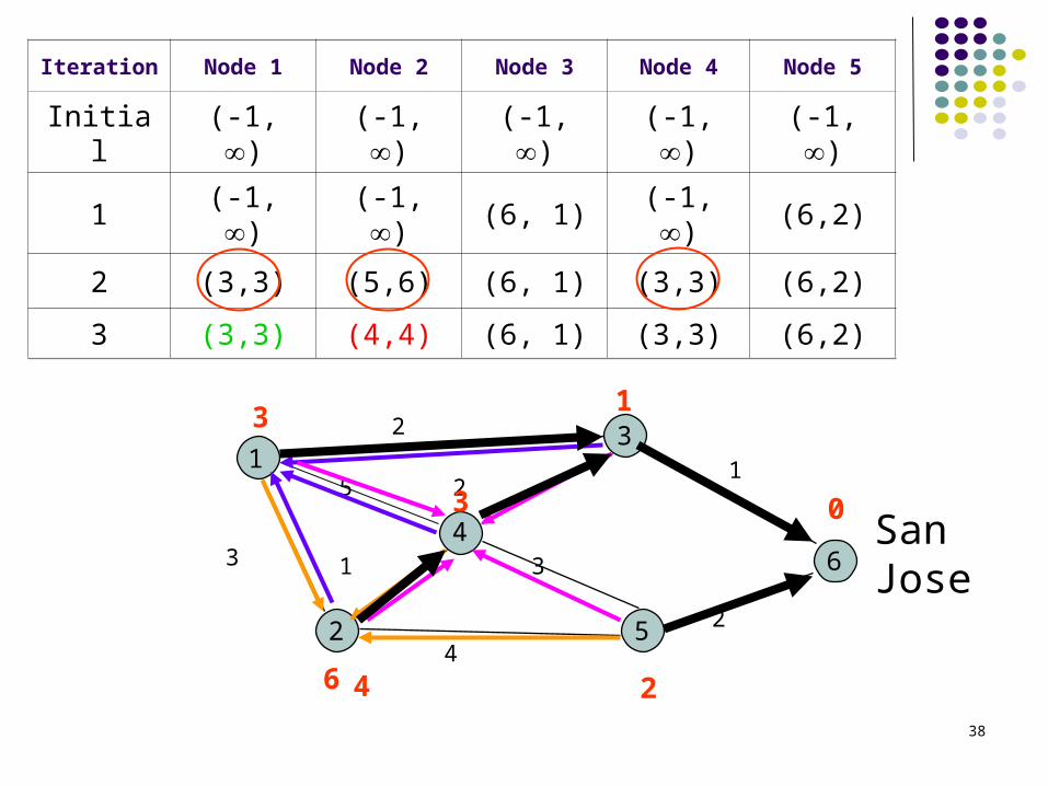
Iteration Node 1 Node 2 Node 3 Node 4 Node 5
Initial (-1, ) (-1, ) (-1, ) (-1, ) (-1, )
1 (-1, ) (-1, ) (6, 1) (-1, ) (6,2)
2 (3,3) (5,6) (6, 1) (3,3) (6,2)
3 (3,3) (4,4) (6, 1) (3,3) (6,2)
SanJose
31
5
46
2
2
3
4
2
1
1
2
3
50
1
26
3
3
4
39
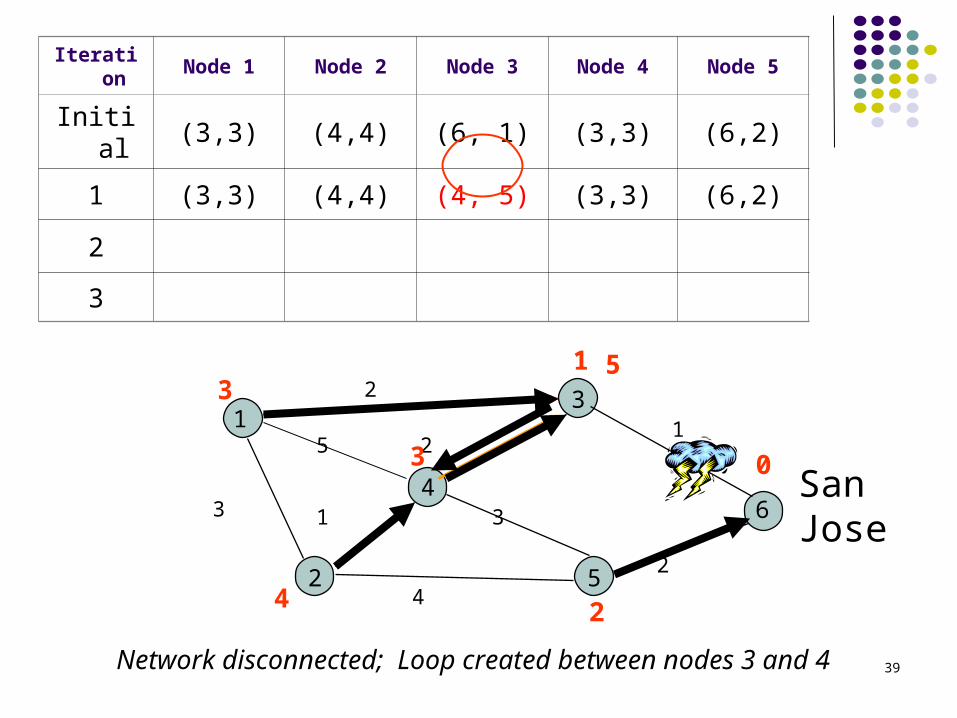
Iteration Node 1 Node 2 Node 3 Node 4 Node 5
Initial (3,3) (4,4) (6, 1) (3,3) (6,2)
1 (3,3) (4,4) (4, 5) (3,3) (6,2)
2
3
SanJose
31
5
46
2
2
3
4
2
1
1
2
3
50
1
2
3
3
4
Network disconnected; Loop created between nodes 3 and 4
5
40
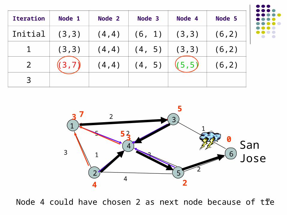
Iteration Node 1 Node 2 Node 3 Node 4 Node 5
Initial (3,3) (4,4) (6, 1) (3,3) (6,2)
1 (3,3) (4,4) (4, 5) (3,3) (6,2)
2 (3,7) (4,4) (4, 5) (5,5) (6,2)
3
SanJose
31
5
46
2
2
3
4
2
1
1
2
3
50
2
5
3
3
4
7
5
Node 4 could have chosen 2 as next node because of tie
41
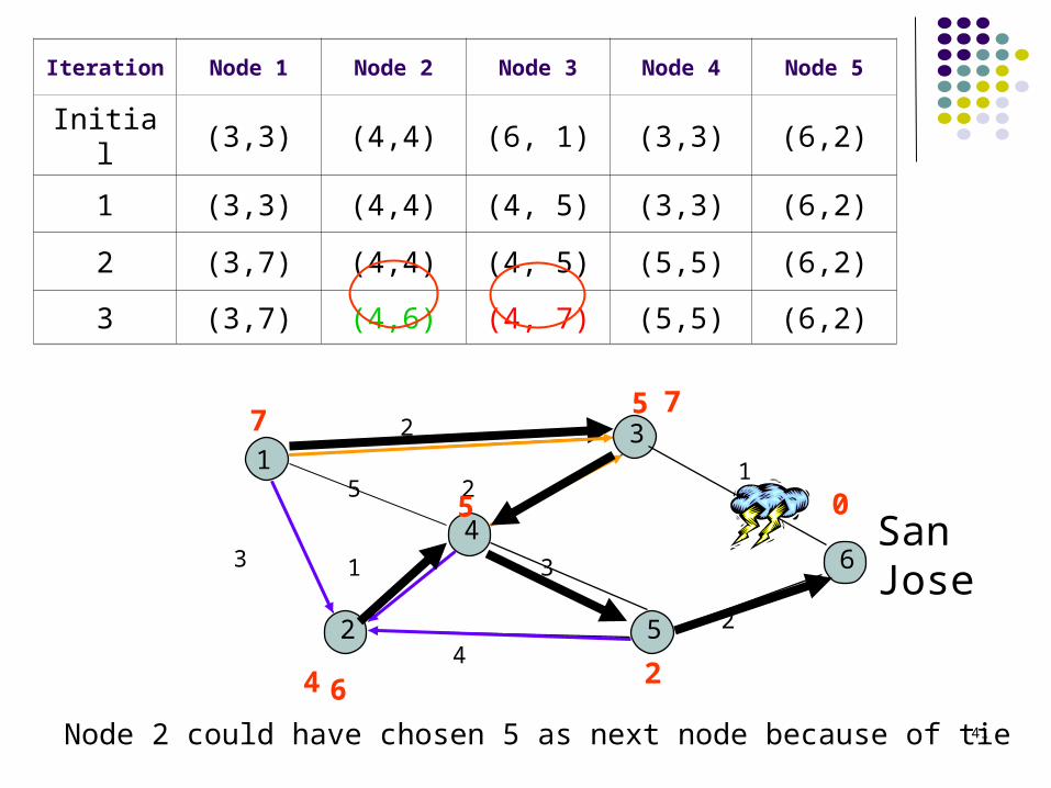
Iteration Node 1 Node 2 Node 3 Node 4 Node 5
Initial (3,3) (4,4) (6, 1) (3,3) (6,2)
1 (3,3) (4,4) (4, 5) (3,3) (6,2)
2 (3,7) (4,4) (4, 5) (5,5) (6,2)
3 (3,7) (4,6) (4, 7) (5,5) (6,2)
SanJose
31
5
46
2
2
3
4
2
1
1
2
3
50
2
5
57
4
7
6
Node 2 could have chosen 5 as next node because of tie
42
3
5
46
2
2
3
4
2
1
1
2
3
51
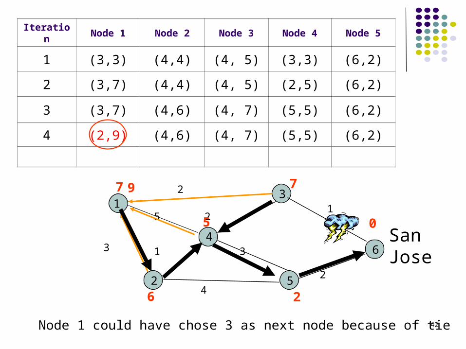
Iteration Node 1 Node 2 Node 3 Node 4 Node 5
1 (3,3) (4,4) (4, 5) (3,3) (6,2)
2 (3,7) (4,4) (4, 5) (2,5) (6,2)
3 (3,7) (4,6) (4, 7) (5,5) (6,2)
4 (2,9) (4,6) (4, 7) (5,5) (6,2)
SanJose
0
77
5
6
9
2
Node 1 could have chose 3 as next node because of tie
43
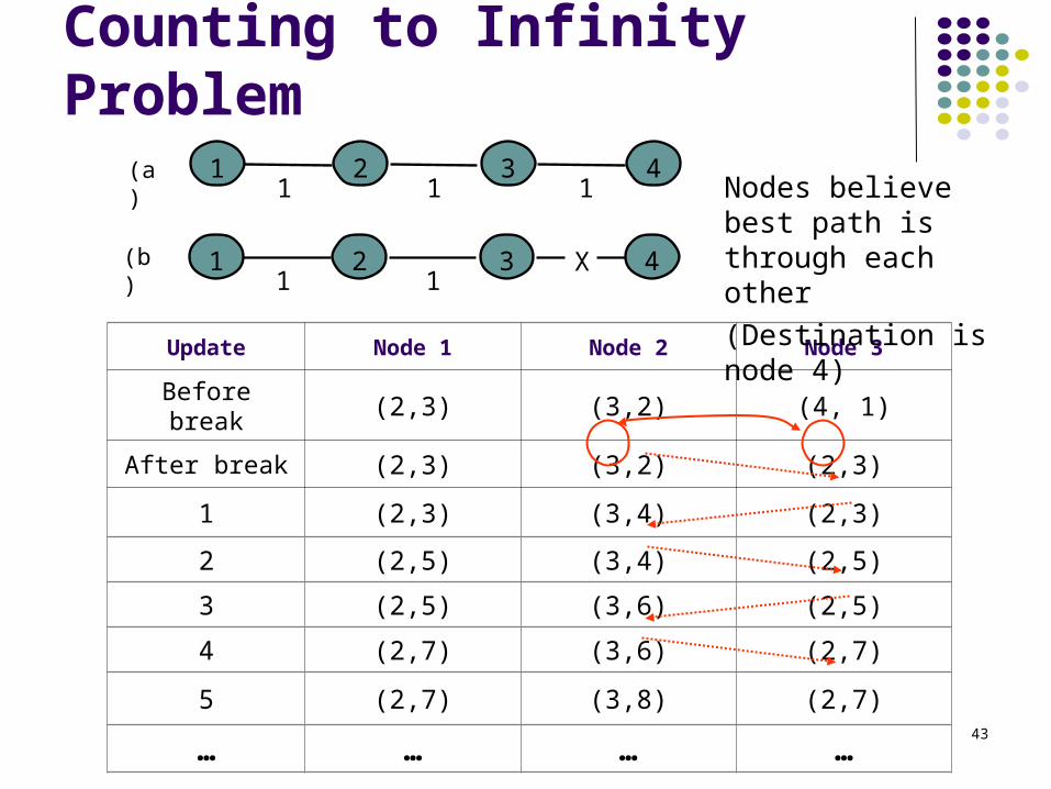
31 2 41 1 1
31 2 41 1
X
(a)
(b)
Update Node 1 Node 2 Node 3
Before break (2,3) (3,2) (4, 1)
After break (2,3) (3,2) (2,3)
1 (2,3) (3,4) (2,3)
2 (2,5) (3,4) (2,5)
3 (2,5) (3,6) (2,5)
4 (2,7) (3,6) (2,7)
5 (2,7) (3,8) (2,7)
… … … …
Counting to Infinity Problem
Nodes believe best path is through each other
(Destination is node 4)
44
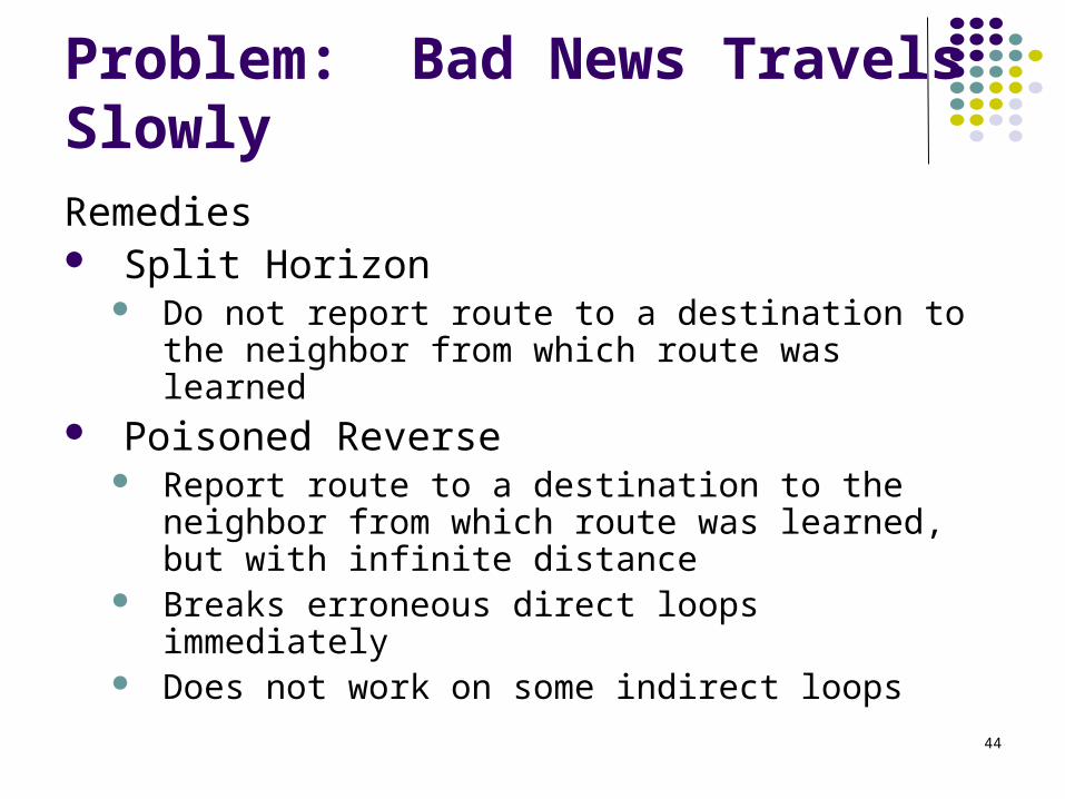
Problem: Bad News Travels Slowly
Remedies Split Horizon
Do not report route to a destination to the neighbor from which route was learned
Poisoned Reverse Report route to a destination to the neighbor
from which route was learned, but with infinite distance
Breaks erroneous direct loops immediately Does not work on some indirect loops
45
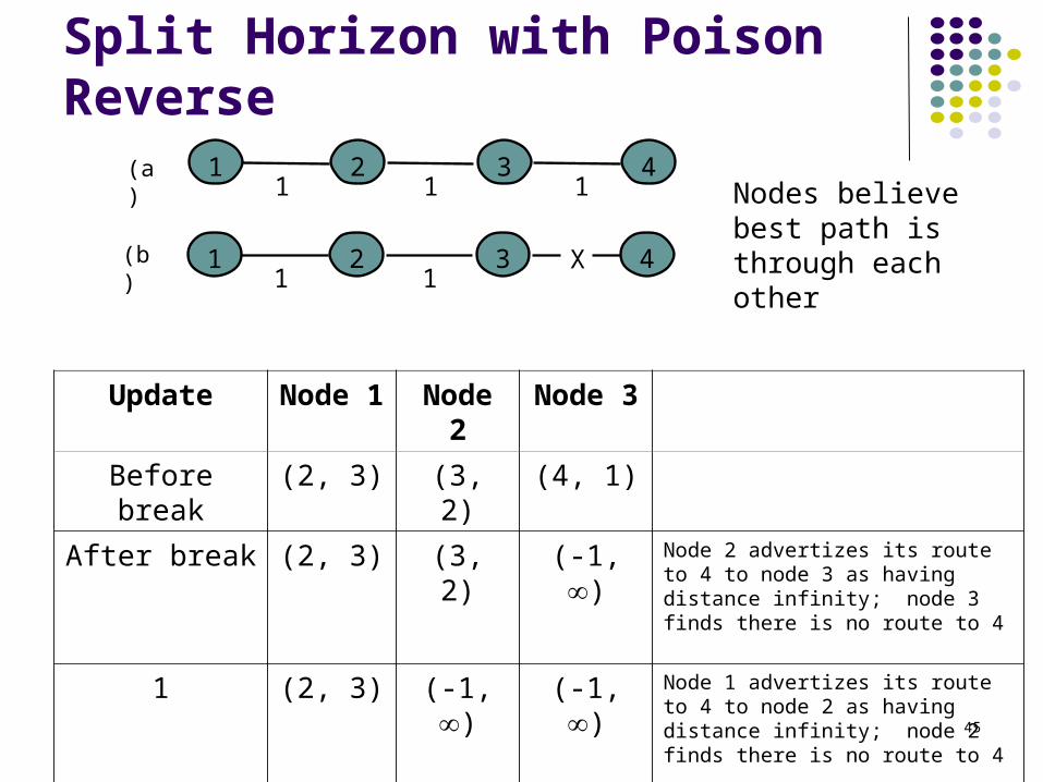
31 2 41 1 1
31 2 41 1
X
(a)
(b)
Split Horizon with Poison Reverse
Nodes believe best path is through each other
Update Node 1 Node 2 Node 3
Before break (2, 3) (3, 2) (4, 1)
After break (2, 3) (3, 2) (-1, ) Node 2 advertizes its route to 4 to node 3 as having distance infinity; node 3 finds there is no route to 4
1 (2, 3) (-1, ) (-1, ) Node 1 advertizes its route to 4 to node 2 as having distance infinity; node 2 finds there is no route to 4
2 (-1, ) (-1, ) (-1, ) Node 1 finds there is no route to 4
46
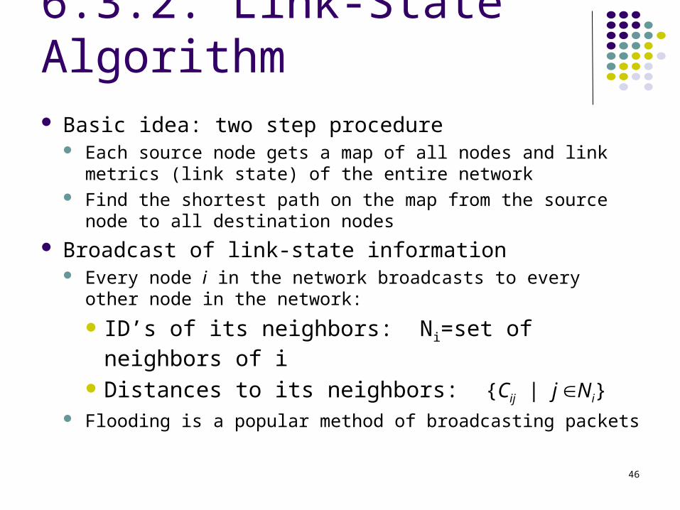
6.3.2. Link-State Algorithm Basic idea: two step procedure
Each source node gets a map of all nodes and link metrics (link state) of the entire network
Find the shortest path on the map from the source node to all destination nodes
Broadcast of link-state information Every node i in the network broadcasts to every other node
in the network:
ID’s of its neighbors: Ni=set of neighbors of i
Distances to its neighbors: {Cij | j Ni} Flooding is a popular method of broadcasting packets
47
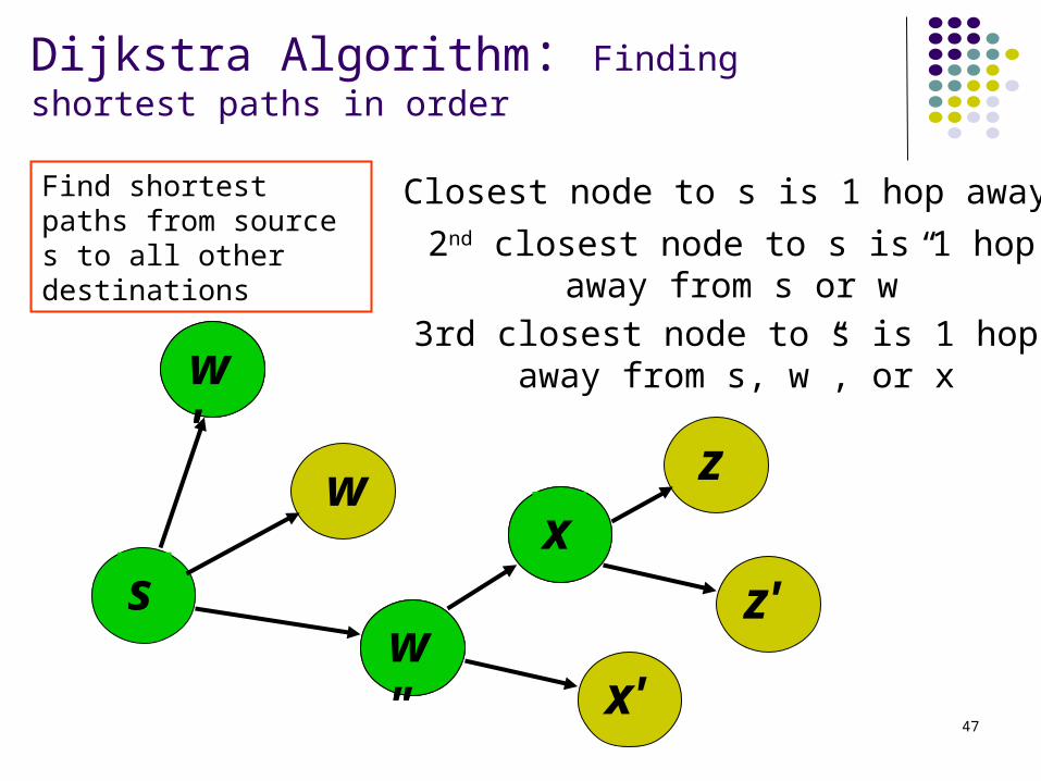
Dijkstra Algorithm: Finding shortest paths in order
s
w
w"
w'
Closest node to s is 1 hop away
w"
x
x'
2nd closest node to s is 1 hop away from s or w”
xz
z'
3rd closest node to s is 1 hop away from s, w”, or xw
'
Find shortest paths from source s to all other destinations
48
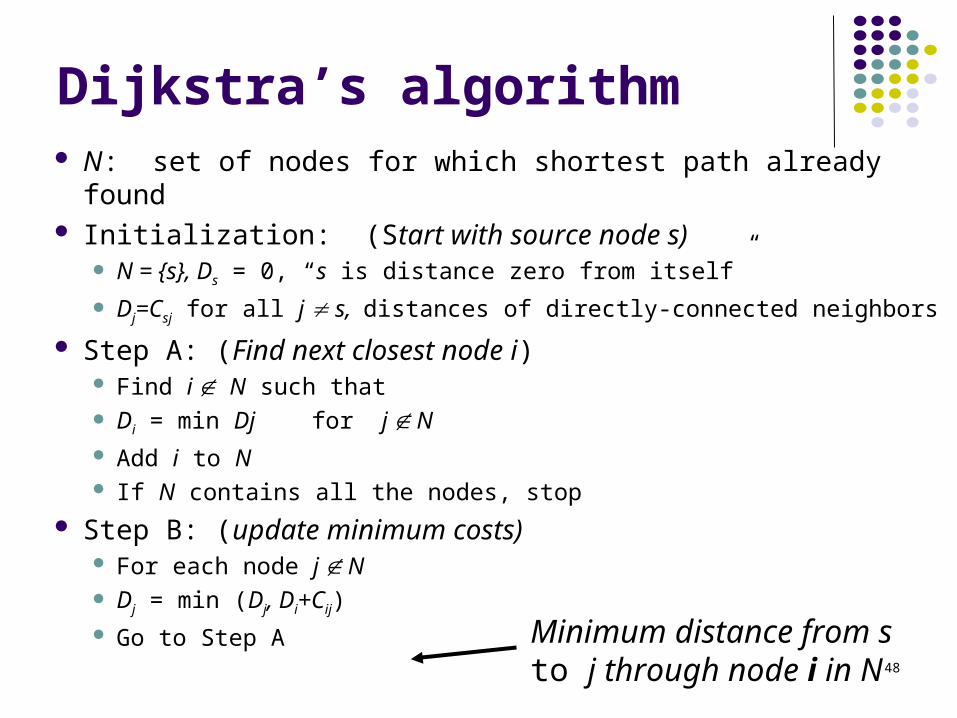
Dijkstra’s algorithm N: set of nodes for which shortest path already found Initialization: (Start with source node s)
N = {s}, Ds = 0, “s is distance zero from itself”
Dj=Csj for all j s, distances of directly-connected neighbors
Step A: (Find next closest node i) Find i N such that Di = min Dj for j N Add i to N If N contains all the nodes, stop
Step B: (update minimum costs) For each node j N Dj = min (Dj, Di+Cij) Go to Step A
Minimum distance from s to j through node i in N
49
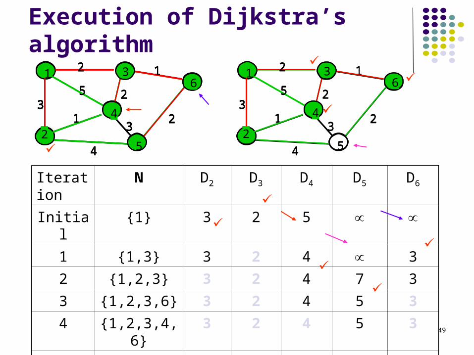
Execution of Dijkstra’s algorithm
Iteration N D2 D3 D4 D5 D6
Initial {1} 3 2 5 1 {1,3} 3 2 4 3
2 {1,2,3} 3 2 4 7 3
3 {1,2,3,6} 3 2 4 5 3
4 {1,2,3,4,6} 3 2 4 5 3
5 {1,2,3,4,5,6} 3 2 4 5 3
1
2
4
5
6
1
1
2
32
35
2
4
3 1
2
4
5
6
1
1
2
32
35
2
4
331
2
4
5
6
1
1
2
32
35
2
4
3 1
2
4
5
6
1
1
2
32
35
2
4
331
2
4
5
6
1
1
2
32
35
2
4
33 1
2
4
5
6
1
1
2
32
35
2
4
331
2
4
5
6
1
1
2
32
35
2
4
33
50
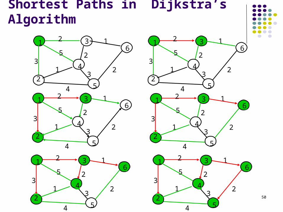
Shortest Paths in Dijkstra’s Algorithm
1
2
4
5
6
1
1
2
32
35
2
4
3 31
2
4
5
6
1
1
2
32
35
2
4
3
1
2
4
5
6
1
1
2
32
35
2
4
33 1
2
4
5
6
1
1
2
32
35
2
4
33
1
2
4
5
6
1
1
2
32
35
2
4
33 1
2
4
5
6
1
1
2
32
35
2
4
33
51
Reaction to Failure
If a link fails, Router sets link distance to infinity & floods the
network with an update packet All routers immediately update their link database &
recalculate their shortest paths Recovery very quick
But watch out for old update messages Add time stamp or sequence # to each update
message Check whether each received update message is new If new, add it to database and broadcast If older, send update message on arriving link
52
Why is Link State Better?
Fast, loopless convergence Support for precise metrics, and multiple
metrics if necessary (throughput, delay, cost, reliability)
Support for multiple paths to a destination algorithm can be modified to find best two paths
53
Topic 6: Routing (Network Layer)
Reference
Leon-Garcia and I. Widjaja, Communication Networks, pp. 492-495, 515-520, 522-534.
(Reserved in the DC library. Call No. TK5105. L46 2004.)