Embed Size (px)
Citation preview
Network Formation with Local Complements and Global Substitutes: TheCase of R&D NetworksI
Chih-Sheng Hsieha, Michael D. Königb, Xiaodong Liuc
aDepartment of Economics, Chinese University of Hong Kong, CUHK Shatin, Hong Kong, China.bDepartment of Economics, University of Zurich, Schönberggasse 1, CH-8001 Zurich, Switzerland.
cDepartment of Economics, University of Colorado Boulder, Boulder, Colorado 80309–0256, United States.
Abstract
We introduce a stochastic network formation model where agents choose both actions and links.Neighbors in the network benefit from each other’s action levels through local complementari-ties and there exists a global interaction effect reflecting a strategic substitutability in actions.We provide a complete equilibrium characterization in the form of a Gibbs measure, and showthat the model is consistent with empirically observed networks. We then use our equilibriumcharacterization to show that the model can be conveniently estimated even for large networks.The policy relevance is demonstrated with examples of firm exit, mergers and subsidies in R&Dcollaboration networks.Key words: network formation, peer effects, technology spillovers, key player, mergers andacquisitions, subsidiesJEL: C11, C63, C73, D83, L22
IWe would like to thank Anton Badev, Filomena Garcia, David Hemous, Matt Jackson, Terence Johnson, AlexeyKushnir, Lung-Fei Lee, Elena Manresa, Andrea Montanari, Nick Netzer, Onur Özgür, Agnieszka Rusinowska, MaríaSáez-Martí, Armin Schmutzler, Martin Summer, Adam Szeidl, Joachim Voth, Timothy Van Zandt, Yves Zenou,Fabrizio Zilibotti, and seminar participants at the Workshop on Networks: Dynamics, Information, Centrality, andGames at Centre d’Economie de la Sorbonne in Paris, the Second Annual NSF Conference on Network Sciencein Economics at Stanford University, the Econometric Society World Congress in Montreal, the congress of theEuropean Economic Association in Mannheim, the 25th Stony Brook International Conference on Game Theory,the Public Economic Theory Conference in Lisbon, the University of Zurich, Bern, the National Taiwan University,the Austrian National Bank and Stanford University for the helpful comments and advice. We further thankChristian Helmers for data sharing and Sebastian Ottinger for the excellent research assistance. A previous versionof this paper has been circulated under the title “Dynamic R&D Networks” as Working Paper No. 109 in theDepartment of Economics working paper series of the University of Zurich. Michael König acknowledges financialsupport from Swiss National Science Foundation through research grants PBEZP1–131169 and 100018_140266,and thanks SIEPR and the Department of Economics at Stanford University for their hospitality during 2010–2012.
Email addresses: [email protected] (Chih-Sheng Hsieh), [email protected] (Michael D.König), [email protected] (Xiaodong Liu)
This version: October 13, 2017, First version: April 24, 2012
1. Introduction
Networks are important in shaping individual behavior and aggregate outcomes in many social andeconomic applications [Jackson, 2008; Jackson et al., 2017]. A crucial aspect of such environmentsis the coevolution of networks and behaviors: an agent in a network adjust his behavior based onthose of his connections and he choose his connections based on their behaviors. In this paperwe introduce a tractable framework to study the joint evolution of networks and behaviors whichcan be applied to real world networks and used for policy analysis.
We consider a general linear-quadratic interdependent utility function [Ballester et al., 2006],where agents choose action levels and create links at a cost. Neighbors in the network benefit fromeach other’s action levels through local complementarities, such as those that arise between R&Dcollaborating firms sharing knowledge about a cost-reducing technology. The global interactioneffect reflects a strategic substitutability in actions, for example, through business stealing effectsthat arise when a firm expands its production in the market. The tractability of the model allowsus to provide a complete equilibrium characterization, and an efficiency analysis. Moreover, itis shown that the equilibrium networks generated by the model consistently reproduce featuresof real world networks. Further, using the equilibrium characterization in the form of a Gibbsmeasure, we show that the model can be conveniently estimated even for large networks. Finally,the model is amenable to policy analysis, and we illustrate this with examples of firm exits,mergers and acquisitions (M&A) and subsidies in the context of R&D collaboration networks.
Overview of the results and contributions Our paper attempts to make three interrelatedcontributions: a theoretical, an econometric and a policy contribution. Our model has a broadrange of applications in various fields [Jackson et al., 2015]. To give a concrete example, in thefollowing we will illustrate our contributions with the example of firms forming R&D collabo-rations to benefit from technology spillovers while, at the same time, being competitors in theproduct market [D’Aspremont and Jacquemin, 1988].
First, this paper provides the first fully tractable and estimable model of strategic R&Dnetwork formation with endogenous production and R&D collaboration choices, which takes intoaccount the two-way flow of influence from the market structure to the incentives to form R&Dcollaborations and, in turn, from the formation of collaborations to the market structure.
We study the incentives of firms to form R&D collaborations with other firms and the im-plications of these alliance decisions for the overall market structure. We introduce a dynamicprocess in which firms can adjust both, quantities produced (as well as R&D efforts), and theR&D collaborations between them, based on a noisy profit maximization rationale [Blume, 2003;Brock and Durlauf, 2001], taking into account that the establishment of an R&D collaborationis fraught with ambiguity and uncertainty [see e.g., Czarnitzki et al., 2015; Kelly et al., 2002].Using a potential function we show that the stationary states of this process are completely char-acterized by a “Gibbs measure” [Bisin et al., 2006; Grimmett, 2010]. Moreover, we show thatwhen firms have heterogeneous marginal costs stemming from differences in their productivity,then the stochastically stable networks (in the limit of vanishing noise) are “nested split graphs”[König et al., 2014a],1 providing an explanation for why nestedness has been observed in empir-
1A network is a nested split graph if the neighborhood of every node is contained in the neighborhoods ofthe nodes with higher degrees [Mahadev and Peled, 1995]. See supplementary Appendix B for further network
1
ical R&D networks [Tomasello et al., 2016]. Nested split graphs further have a core-peripherystructure, which has also been documented in empirical studies on R&D networks [Kitsak et al.,2010; Rosenkopf and Schilling, 2007]. In particular, Kitsak et al. [2010] find that firms in thecore have a higher market value, consistent with the predictions of our model. Next, we showthat when firms’ productivities are Pareto distributed, then the firms’ output levels and degreesalso follow a Pareto distribution, which is consistent with the empirical data [Powell et al., 2005].Further, we find that there exists a sharp transition between sparse and dense networks withdecreasing linking costs. We also compute the stationary output levels and show that there existsan intermediate range of the linking cost for which multiple equilibria arise. The equilibriumselection is a path dependent process characterized by “hysteresis” [David, 1992]. Moreover, asin the case of the network density, there exists a sharp transition from a low output to a highoutput equilibrium.
It is also possible to generalize our model by introducing heterogeneous spillovers from collabo-rations between firms with differences in their technological characteristics, and/or heterogeneouscosts of collaboration. In particular, assuming that firms can only benefit from collaborationsif they have at least one technology in common, we show that our model is a generalization ofa “random intersection graph” [Deijfen and Kets, 2009],2 for which positive degree correlations(assortativity) can be obtained. We then investigate the efficient network and output structurethat maximize social welfare, and find that equilibrium networks tend to be under-connected,compared to the social optimum.3
Second, we bring the model to the data by analyzing a unique dataset of firm R&D collabora-tions matched to firms’ balance sheets. The theoretical characterization of the stationary statesvia a Gibbs measure allows us to estimate the model’s parameters using a Markov Chain MonteCarlo (MCMC) method called double Metropolis-Hastings (DMH) algorithm [Hsieh and Lee,2013; Mele, 2017; Liang, 2010], which can handle the problem of the “intractable normalizationconstant” in the probability likelihood function by introducing auxiliary network and outcomedata.4 We further use a novel adaptive exchange (AEX) algorithm to overcome the slow mixingproblem faced by the DMH algorithm [Jin et al., 2013; Liang et al., 2015]. It applies importancesampling to prevent the “local trap problem” when the likelihood represented by the Gibbs mea-sure is multi-modal. We also propose a likelihood partition approach in which we “integrate out”the intractable normalizing constant by direct analytic computations. The resulting likelihoodallows us to use a standard MH algorithm for estimation, and this approach can be efficientlyapplied to large networks.
From our estimation results we observe that the estimated technology spillover effect is signif-icantly positive and the estimated competition effect is significantly negative, which confirms ourtheoretical predictions that firms face a positive complementary effect from R&D collaborationsand a negative substitution effect from competing firms in the same market. We also investigate
definitions and characterizations.2A random intersection graph is constructed by assigning to each node a subset of a given set and two nodes
are connected when their respective subsets intersect.3In Section 4.3 we analyze the effectiveness of a subsidy on firms’ R&D collaboration costs, that gives firms
incentives to form collaborations and thus increases the network connectivity.4The intractable normalization constant refers to the denominator of the Gibbs likelihood function. The de-
nominator involves a summation over all possible network configurations. If there are n nodes, then there are 2(ns)
possible networks to consider.
2
heterogeneous technology spillovers by weighting the R&D collaboration links with Jaffe and Ma-halanobis technology proximity measures [Bloom et al., 2013]. The results show variations on theestimated spillover effects in correspondence with the average magnitudes of different proximitymeasures.
Third, we use our estimated model to investigate the impact of exogenous shocks on thenetwork. In particular, we perform a “key player” analysis [Ballester et al., 2006; Zenou, 2015],to gauge the impact of firm exit on the economy, when firms are connected through R&D col-laborations in a network.5 The exit of a firm could be due to either financial reasons, such asthe recession experienced by the American automobile manufacturing industry during the globalfinancial downturn, or legal reasons, such as the recent emission-fraud scandal of Volkswagen.In the latter case, policy makers want to know the overall cost they impose on the economy byinflicting high pollution penalties and criminal fines that might threaten the continued existenceof a firm. Focusing on the chemicals and pharmaceutical sector, our results indicate that the exitof Amgen, an American global pharmaceutical corporation, would lead to a reduction in welfareof 3.7%. We then provide a ranking of the firms in our sample according to their impact onwelfare upon exit. The ranking shows that the most important firms are not necessarily the oneswith the highest market share, but that we need to take into account the positions of these firmsin a network of R&D collaborations, and how this network dynamically responds to shocks offirm exits.
Our framework also allows us to study mergers and acquisitions, and their impact on welfare[Farrell and Shapiro, 1990]. Traditional market concentration indices are not adequate to correctlyaccount for the network effect of a merger on welfare [Encaoua and Hollander, 2002]. This isbecause the effect of a merger on industry profits, consumer surplus and overall welfare dependsnot only on the market structure, but also on the architecture of the R&D collaboration networkbetween firms through which R&D spillovers are channelled. In such networked markets benefitsfrom concentration of R&D activities can arise through economies of scale and faster diffusion oftechnologies in more centralized networks [Daughety, 1990].
By taking into account the network effect our results show that a merger between DaiichiSankyo Co. Ltd., the second largest pharmaceutical company in Japan and Schering-PloughCorp., a U.S.-based multinational pharmaceutical company, would result in a welfare loss of0.6%. In contrast, a welfare gain of 0.86% from a merger is obtained between Isis Pharm. Inc.and Takeda Pharm. Inc. Comparing the firms involved in mergers that lead to welfare gainsas opposed to the ones that lead to welfare losses, we see that mergers between firms with alarger number of patents and a larger number of R&D collaborations typically lead to welfaregains, while mergers between firms with few collaborations, fewer patents and a larger marketshare typically lead to a welfare loss. This indicates that the R&D spillover effect is largerwhen two well connected, R&D intensive firms merge, while welfare losses from increased marketconcentration dominate when less connected and more market dominant firms are involved in themerger. Our counterfactual policy analysis is therefore potentially important for antitrust policymakers.
Finally, we investigate the impact of subsidizing R&D collaboration costs of selected pairs of
5We note that our model is formulated in a fairly flexible way, and because we consider the general payoffstructure introduced in Ballester et al. [2006], one could use our framework also to investigate key players incriminal networks, or other related contexts [see also Zenou, 2015].
3
firms. Our study indicates that subsidizing an R&D collaboration between Dynavax Technologies,a U.S.-based biopharmaceutical company, and Shionogi & CO. Ltd., a Japanese pharmaceuticalcompany, would increase welfare by 0.76%. Not taking into account the endogeneity of thenetwork would yield much lower welfare gains. As subsidies are increasingly being used bygovernmental organizations to stimulate collaborative R&D activities, our framework could assistgovernmental funding agencies that typically do not take into account the aggregate spilloversgenerated within a dynamic R&D network structure.
Related literature There is a growing literature on the stochastic evolution of networks goingback to Jackson and Watts [2002],6 using tools from evolutionary game theory [Blume, 1993;Kandori et al., 1993; Sandholm, 2010] to analyze the formation of social and economic networks.In this literature agents form links over time based on myopic improvements that the resultingnetwork offers them relative to the current network. While there is a small probability of mistakes,the stochastically stable states are identified when this probability vanishes. Our paper usessimilar techniques to analyze the stationary states in a stochastic network formation model, butdifferent from the above mentioned works, we investigate the coevolution of links and actions,and develop an estimable framework from our theory that can be applied to real world networks.
There also exist related studies on the formation of R&D networks in the economics literature.Similar to our framework, Goyal and Moraga-Gonzalez [2001], Dawid and Hellmann [2014], andWestbrock [2010] study the formation of R&D networks in which firms can form collaborations toreduce their production costs. In particular, Dawid and Hellmann [2014] study a perturbed bestresponse dynamic process as we do here, and analyze the stochastically stable states. However,different from the current model, they ignore the R&D investment decision, and the technologyspillovers from a collaboration in these models is independent of the identity and the character-istics of the firms involved.7
Similarly, Ehrhardt et al. [2008] analyze the formation of a network in which agents playa coordination game with their neighbors, while König et al. [2014a], Marsili et al. [2004], andFosco et al. [2010] study the coevolution of networks and behavior. As in the present paper, theseauthors show that the interplay between action choice and link creation may feed on each otherto generate sharp transitions from sparse to dense networks. The underlying payoff structure,however, is different from ours. Further, while these authors assume that links decay at random,here link removal depends on whether the agents find this profitable.
Our analysis also bears similarities with a number of other recent contributions in the literaturewhich analyze a similar payoff structure. In the paper by Ballester et al. [2006], the authors deriveequilibrium outcomes in a linear quadratic game where agents’ efforts are local complements in anexogenously given network. Different from Ballester et al. [2006], we make the network as well aseffort choices endogenous.8 Cabrales et al. [2011] allow the network to be formed endogenously,
6For more recent contributions to this literature see, for example, Hojman and Szeidl [2006], Feri [2007] andDawid and Hellmann [2014].
7Goyal and Moraga-Gonzalez [2001] present a more general setup which relaxes this assumption but theiranalysis is restricted to regular graphs and networks comprising of four firms. In this paper we take into accountgeneral equilibrium structures with an arbitrary number of firms and make no ex ante restriction on the potentialcollaboration pattern between them.
8It is straightforward to see that the results obtained in this paper can be generalized to the payoff structureintroduced in Ballester et al. [2006]. See in particular the general payoff structure considered in Equation (1). Weprovide a complete equilibrium characterization for the model introduced in Ballester et al. [2006], but allow both
4
but assume that link strengths are proportional to effort levels, while we make the linking decisiondepending on marginal payoffs. Hiller [2013] studies the joint formation of links and actions usinga similar payoff structure as we do here, however, abstracting from any global substitutabilityeffects, and shows that equilibrium networks are nested split graphs [see also König et al., 2014a].Similarly, Belhaj et al. [2016] analyze the design of optimal networks with the same payoff functionbut without global substitutabilities, and show that when the planner chooses links, but not thelevel of output (second best), the optimal network is a nested split graph. We find that when theplanner chooses both actions and links (first best), both equilibrium and efficient structures arenested spit graphs, even when allowing for global substitutes and incorporating heterogeneousfirms, and we provide a more precise equilibrium characterization beyond the general class ofnested split graphs. In particular, we identify conditions under which both the output and thedegree distributions follow a power law, consistent with the empirical data [Gabaix, 2016; Powellet al., 2005].
Our approach is a further generalization of the endogenous network formation mechanismsproposed in Snijders [2001], Chandrasekhar and Jackson [2012], and Mele [2017]. As in thesepapers, we use a potential function to characterize the stationary states [Monderer and Shapley,1996], but here both, the action choices as well as the linking decisions are fully endogenized.Moreover, different from these papers we provide a microfoundation (from a Cournot competitionmodel with externalities) for the potential function. Further, in a recent paper by Badev [2013]a potential function is used to analyze the formation of networks in which agents not only formlinks but also make a binary choice of adopting a certain behavior depending on the choices oftheir neighbors. Different from Badev [2013], we consider a continuum of choices, and provide amicrofoundation derived from the payoff function introduced in Ballester et al. [2006]. Moreover,different from the previous authors we provide an explicit equilibrium characterization, use analternative estimation method (which can also be applied to large networks and addresses the localtrap problem),9 apply our model to a different context, and study a range of novel counterfactualpolicy scenarios. Relatedly, in a recent paper, Hsieh and Lee [2013] apply a potential function to anempirical model of joint network formation and action choices. However, their potential functionis based on a transferable utility function so that linking decisions are based on maximizingaggregate payoffs, while here we consider decentralized link formation between payoff maximizingagents.
Furthermore, Bimpikis et al. [2014] analyze the effect of mergers and acquisitions withinand across different industries using a similar model as we do here. However, neither doestheir analysis incorporate the spillover effects from R&D collaborations, nor do they allow forthese collaborations to respond to a merger. In contrast, our empirical analysis reveals that thenetwork structure of R&D collaborations matters, and that when ignoring the network structurethe impact of mergers is significantly underestimated. Moreover, we find that mergers betweenhighly connected firms can be welfare improving, a feature that would not arise in the absenceof the R&D network. We thus contribute to the ongoing debate about the validity of antitrustpolicies in innovative industries [Encaoua and Hollander, 2002], by adding another dimension
agents’ actions and links to be endogenously determined.9Note also that classical Maximum Likelihood Estimation (MLE) methods such as the one considered in Badev
[2013] are greatly influenced by the choice of initial parameter values, and if these are not close enough to the truevalues, the method may converge to a sub-optimal solution [Airoldi et al., 2009].
5
that explicitly takes into account efficiency gains that can be realized from R&D spillovers acrossfirms.
Finally, in König et al. [2014b] a similar market structure is considered. In particular, theauthors investigate the impact of a subsidy per unit of R&D spent, while here we analyze subsidiesto R&D collaborations directly. Moreover, the authors characterize key firms whose exit wouldhave the largest impact on the output of the economy in the short run, taking the network asgiven. Here we develop a long run analysis, where the network is allowed to dynamically adjustupon the exit of a firm. To the best of your knowledge, this is the first paper to perform such adynamic key player analysis in a fully strategic environment.
Organization of the paper The paper is organized as follows. The theoretical model isoutlined in Section 2. In particular, Section 2.1 introduces the linear-quadratic payoff functionconsidered in this paper. Section 2.2 defines the stochastic network formation and output adjust-ment process and provides a complete characterization of the stationary state. In Section 2.3 thewelfare maximizing networks are derived. Section 2.4 discusses several extensions of the modelthat allow for firm heterogeneity. Next, Section 3 provides information about the data that weuse and explains the estimation methods and results. Section 4 then uses the estimated model toanalyze several counterfactual policy experiments. Finally, Section 5 concludes. All proofs arerelegated to Appendix A.
Additional relevant material can be found in the supplementary appendices. In particular,supplementary Appendix B provides basic definitions and characterizations of networks. Supple-mentary Appendix C provides a motivation for the linear quadratic payoff function from a modelof R&D collaborating firms that are competing on the product market à la Cournot. Supple-mentary Appendix D explains the distinction between continuous and discrete quantity choices.Supplementary Appendix E explains in detail the extensions mentioned in the main text. Supple-mentary Appendix F provides a detailed description of the data used for our empirical analysisin Section 3, while supplementary Appendix G provides additional details of the estimation al-gorithms. Supplementary Appendix H provides a simulation study to examine the performanceand consistency of our various estimation algorithms, as well as the impact of missing observa-tions on estimation. Finally, supplementary Appendix I shows the robustness of our results whenanalyzing alternative data.
2. Theoretical Framework
2.1. Payoffs
Each firm (agent) i ∈ N = 1, . . . , n in the network G ∈ Gn selects an output (action) levelqi ∈ Q and obtains a linear-quadratic profit (payoff) πi : Qn × Gn → R given by10
πi(q, G) = ηiqi − νq2i − bqi
n∑j =i
qj + ρ
n∑j=1
aijqiqj − ζdi, (1)
10See also Ballester et al. [2006] and Jackson et al. [2015] for a more general discussion of the payoff functionintroduced in Equation (1).
6
where Q is the (bounded) output choice set of a firm, Gn denotes the set of all graphs with n ≥ 2
nodes, aij = 1 if firms i and j set up a collaboration (0 otherwise) and aii = 0.11 Equation (1)is concave in own output, qi, with parameters ηi ≥ 0 and ν ≥ 0. Moreover, b > 0 is a globalsubstitutability parameter, ρ ≥ 0 a local complementarity parameter, ζ ≥ 0 denotes a fixedlinking cost and di is the number of collaborations of firm i. A derivation of the profit functionin Equation (1) in the context of R&D collaborating firms competing à la Cournot can be foundin supplementary Appendix C.
The profit function introduced in Equation (1) admits a (cardinal) potential function [Mon-derer and Shapley, 1996].
Proposition 1. The profit function of Equation (1) admits a potential game where firms chooseboth output and links with a potential function Φ: Qn × Gn → R given by
Φ(q, G) =
n∑i=1
(ηiqi − νq2i )−b
2
n∑i=1
n∑j =i
qiqj +ρ
2
n∑i=1
n∑j=1
aijqiqj − ζm, (2)
for any q ∈ Qn and G ∈ Gn where m denotes the number of links in G.
The potential function has the property that the marginal profit of a firm from adding orremoving a link is exactly equivalent to the difference in the potential function from addingor removing a link. Similarly, the marginal profit of a firm from changing its output level isexactly equivalent to the change of the potential function.12 The potential function thus allowsto aggregate the incentives of the firms to either change their links or adjust their production levelsin a single global function. The existence of a potential function will be crucial for the equilibriumcharacterization of the network formation process that will be introduced in the following section.
2.2. Network Dynamics and Equilibrium Characterization
In this section we introduce a dynamic model where firms choose both output and links, basedon the profit function of Equation (1). In this model the network is formed endogenously, basedon the decisions of firms with whom to collaborate,13 and share knowledge about a cost reducingtechnology. The opportunities for change arrive as a Poisson process [Blume, 1993; Sandholm,2010], similar to Calvo models of pricing [Calvo, 1983]. As in the best reply dynamics analyzedin Cournot [1838],14 when a firm receives such an opportunity to change it adjusts its outputor collaborations so as to maximize its profit while taking the output levels and collaborationsof the other firms as given, assuming that firms are myopic (also see e.g., Jackson and Watts[2002]; Watts [2001]).15 To capture the fact that R&D projects and the establishment of an R&D
11See supplementary Appendix B for further network definitions and characterizations.12 More formally, the potential Φ has the property that for any q ∈ Qn and G,G′ ∈ Gn with G′ = G⊕ (i, j) or
G′ = G ⊖ (i, j) we have that Φ(q, G′) − Φ(q, G) = πi(q, G′) − πi(q, G), where G ⊕ (i, j) (G ⊖ (i, j)) denotes the
network obtained from G by adding (removing) the link (i, j). Moreover, for qi, q′i ∈ Q, q−i ∈ Qn−1 and G ∈ Gn
we have that Φ(q′i,q−i, G)− Φ(qi,q−i, G) = πi(q′i,q−i, G)− πi(qi,q−i, G).
13Note that the formation of a collaboration requires the mutual agreement of both firms involved in a collabora-tion, while for the termination of a collaboration it is sufficient that one of the firms finds this profitable [Jacksonand Watts, 2002].
14Cournot [1838] analyzed a dynamic process in which firms myopically best respond in the current period tothe existing output levels of all rivals. See also Daughety [2005].
15The assumption of myopic firms is also common in boundedly rational dynamic decision-making, as consideredin Gabaix [2014].
7
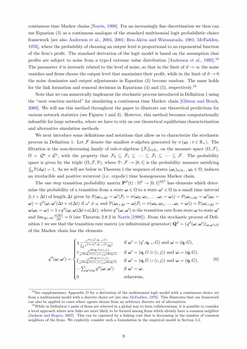
collaboration are fraught with ambiguity and uncertainty [Czarnitzki et al., 2015; Kelly et al.,2002], we will introduce noise in this decision process. The precise definition of the dynamics ofoutput adjustment and network evolution is given in the following.
Definition 1 (Cournot Best Reply Dynamics). The evolution of the population of firms andthe collaborations between them is characterized by a sequence of states (ωt)t∈R+, ωt ∈ Ω =Qn×Gn, where each state ωt = (qt, Gt) consists of a vector of firms’ output levels, qt ∈ Qn, anda network of collaborations, Gt ∈ Gn. We assume that firms choose quantities from a bounded setQ. In a short time interval [t, t+∆t), t ∈ R+, one of the following events happens:
Output adjustment At rate χ ≥ 0 a firm i ∈ N is selected at random and given an adjustmentopportunity of its current output level. When firm i receives such an adjustment opportunity,the probability to choose a certain output level is governed by a multinomial logistic functionwith choice set Q and parameter ϑ, so that the probability that we observe a switch by firm ito an output level q conditional on the output levels of all other firms, q−it, and the network,Gt, at time t is given by16
P (ωt+∆t = (q,q−it, Gt)|ωt = (qt, Gt)) = χeϑπi(q,q−it,Gt)∫
Q eϑπi(q′,q−it,Gt)dq′
∆t+ o(∆t). (3)
Link formation With rate τ ≥ 0 a pair of firms i, j which is not already connected receivesan opportunity to form a link. The formation of a link depends on the marginal profitsthe firms receive from the link plus an additive pairwise i.i.d. error term εij,t. The prob-ability that link (i, j) is created is then given byP (ωt+∆t = (qt, Gt ⊕ (i, j))|ωt = (qt, Gt)) =τ P (πi(qt, Gt ⊕ (i, j))− πi(qt, Gt) + εij,t > 0 ∩ πj(qt, Gt ⊕ (i, j))− πj(qt, Gt) + εij,t > 0)∆t+o(∆t). Using the fact that πi(qt, Gt ⊕ (i, j)) − πi(qt, Gt) = πj(qt, Gt ⊕ (i, j)) − πj(qt, Gt) =Φ(qt, Gt⊕(i, j))−Φ(qt, Gt), and assuming that the error term εij,t is independently logisticallydistributed,17 we obtain
P (ωt+∆t = (qt, Gt ⊕ (i, j))|ωt = (qt, Gt)) = τeϑΦ(qt,Gt⊕(i,j))
eϑΦ(qt,Gt⊕(i,j)) + eϑΦ(qt,Gt)∆t+ o(∆t). (4)
Link removal With rate ξ ≥ 0 a pair of connected firms i, j receives an opportunity to ter-minate their collaboration. The link is removed if at least one firm finds this profitable.The marginal profits from removing the link (i, j) are perturbed by an additive pairwisei.i.d. error term εij,t. The probability that the link (i, j) is removed is then given byP (ωt+∆t = (qt, Gt ⊖ (i, j))|ωt = (qt, Gt)) = ξ P(πi(qt, Gt ⊖ (i, j)) − πi(qt, Gt) + εij,t > 0 ∪πj(qt, Gt⊖ (i, j))− πj(qt, Gt) + εij,t > 0)∆t+ o(∆t). Using the fact that πi(qt, Gt⊖ (i, j))−πi(qt, Gt) = πj(qt, Gt ⊖ (i, j))− πj(qt, Gt) = Φ(qt, Gt ⊖ (i, j))−Φ(qt, Gt), and assuming thatthe error term is independently logistically distributed we obtain
P (ωt+∆t = (qt, Gt ⊖ (i, j))|ωt = (qt, Gt)) = ξeϑΦ(qt,Gt⊖(i,j))
eϑΦ(qt,Gt⊖(i,j)) + eϑΦ(qt,Gt)∆t+ o(∆t). (5)
We assume that the set Q is a discretization of the bounded interval [0, q], with q < ∞.The fact that Q is a countable set allows us to use standard results for discrete state space,
16The multinomial choice probability can be derived from a random utility model where firms maximize profitssubject to a random error term [Anderson et al., 2004; McFadden, 1976]. See supplementary Appendix D for moredetails.
17Let z be i.i. logistically distributed with mean 0 and scale parameter ϑ, i.e. Fz(x) = eϑx
1+eϑx . Consider therandom variable ε = g(z) = −z. Since g is monotonic decreasing, and z is a continuous random variable, thedistribution of ε is given by Fε(y) = 1− Fz(g
−1(y)) = eϑy
1+eϑy .
8
continuous time Markov chains [Norris, 1998]. For an increasingly fine discretization we then canuse Equation (3) as a continuous analogue of the standard multinomial logit probabilistic choiceframework [see also Anderson et al., 2004, 2001; Ben-Akiva and Watanatada, 1981; McFadden,1976], where the probability of choosing an output level is proportional to an exponential functionof the firm’s profit. The standard derivation of the logit model is based on the assumption thatprofits are subject to noise from a type-I extreme value distribution [Anderson et al., 1992].18
The parameter ϑ is inversely related to the level of noise, so that in the limit of ϑ→ ∞ the noisevanishes and firms choose the output level that maximizes their profit, while in the limit of ϑ→ 0
the noise dominates and output adjustments in Equation (3) become random. The same holdsfor the link formation and removal decisions in Equations (4) and (5), respectively.19
Note that we can numerically implement the stochastic process introduced in Definition 1 usingthe “next reaction method” for simulating a continuous time Markov chain [Gibson and Bruck,2000]. We will use this method throughout the paper to illustrate our theoretical predictions forvarious network statistics (see Figures 1 and 3). However, this method becomes computationallyinfeasible for large networks, where we have to rely on our theoretical equilibrium characterizationand alternative simulation methods.
We next introduce some definitions and notations that allow us to characterize the stochasticprocess in Definition 1. Let F denote the smallest σ-algebra generated by σ (ωt : t ∈ R+). Thefiltration is the non-decreasing family of sub-σ-algebras Ftt∈R+ on the measure space (Ω,F),Ω = Qn × Gn, with the property that F0 ⊆ F1 ⊆ · · · ⊆ Ft ⊆ · · · ⊆ F . The probabilityspace is given by the triple (Ω,F ,P), where P : F → [0, 1] is the probability measure satisfying∫Ω P(dω) = 1. As we will see below in Theorem 1 the sequence of states (ωt)t∈R+ , ωt ∈ Ω, induces
an irreducible and positive recurrent (i.e. ergodic) time homogeneous Markov chain.The one step transition probability matrix Pϑ(t) : Ω2 → [0, 1]|Ω|2 has elements which deter-
mine the probability of a transition from a state ω ∈ Ω to a state ω′ ∈ Ω in a small time interval[t, t+∆t) of length ∆t given by P(ωt+∆t = ω′|Ft = σ(ω0,ω1, . . . ,ωt = ω)) = P(ωt+∆t = ω′|ωt =ω) = qϑ(ω,ω′)∆t+ o(∆t) if ω′ = ω and P(ωt+∆t = ω|Ft = σ(ω0,ω1, . . . ,ωt = ω)) = P(ωt+∆t =
ω|ωt = ω) = 1+qϑ(ω,ω)∆t+o(∆t), where qϑ(ω,ω′) is the transition rate from state ω to state ω′
and lim∆t→0o(∆t)∆t = 0 (see Theorem 2.8.2 in Norris [1998]). From the stochastic process of Defi-
nition 1 we see that the transition rate matrix (or infinitesimal generator) Qϑ = (qϑ(ω,ω′))ω,ω′∈Ω
of the Markov chain has the elements
qϑ(ω,ω′) =
χ eϑπi(q′,q−i,G)∫
Q eϑπi(q′′,q−i,G)dq′′
if ω′ = (q′,q−i, G) and ω = (q, G),
τ eϑΦ(q,G⊕(i,j))
eϑΦ(q,G⊕(i,j))+eϑΦ(q,G) if ω′ = (q, G⊕ (i, j)) and ω = (q, G),
ξ eϑΦ(q,G⊖(i,j))
eϑΦ(q,G⊖(i,j))+eϑΦ(q,G) if ω′ = (q, G⊖ (i, j)) and ω = (q, G),
−∑
ω′ =ω qϑ(ω,ω′) if ω′ = ω,
0 otherwise,
(6)
18See supplementary Appendix D for a derivation of the multinomial logit model with a continuous choice setfrom a mulitnomial model with a discrete choice set [see also McFadden, 1976]. This illustrates that our frameworkcan also be applied to cases where agents choose from an arbitrary discrete set of alternatives.
19While in Definition 1 pairs of firms are selected in a global way to form collaborations, it is possible to considera local approach where new links are more likely to be formed among firms which already have a common neighbor[Jackson and Rogers, 2007]. This can be captured by a linking cost that is decreasing in the number of commonneighbors of the firms. We explicitly consider such a formulation in the empirical model in Section 3.2.
9
with∑
ω′∈Ω qϑ(ω,ω′) = 0.20 As the Markov chain is time homogeneous, the transition rates
are independent of time. The stationary distribution µϑ : Ω → [0, 1] is then the solution toµϑPϑ = µϑ, or equivalently µϑQϑ = 0 [Norris, 1998].
With the potential function Φ of Proposition 1 we can compute the stationary distribution inthe form of a Gibbs measure [Grimmett, 2010].
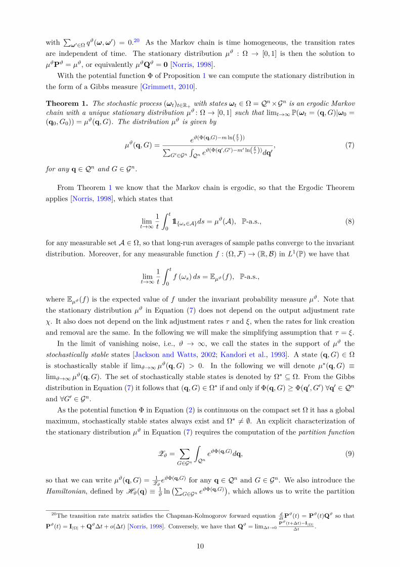
Theorem 1. The stochastic process (ωt)t∈R+ with states ωt ∈ Ω = Qn×Gn is an ergodic Markovchain with a unique stationary distribution µϑ : Ω → [0, 1] such that limt→∞ P(ωt = (q, G)|ω0 =(q0, G0)) = µϑ(q, G). The distribution µϑ is given by
µϑ(q, G) =eϑ(Φ(q,G)−m ln( ξ
τ ))∑G′∈Gn
∫Qn e
ϑ(Φ(q′,G′)−m′ ln( ξτ ))dq′
, (7)
for any q ∈ Qn and G ∈ Gn.
From Theorem 1 we know that the Markov chain is ergodic, so that the Ergodic Theoremapplies [Norris, 1998], which states that
limt→∞
1
t
∫ t
01ωs∈Ads = µϑ(A), P-a.s., (8)
for any measurable set A ∈ Ω, so that long-run averages of sample paths converge to the invariantdistribution. Moreover, for any measurable function f : (Ω,F) → (R,B) in L1(P) we have that
limt→∞
1
t
∫ t
0f (ωs) ds = Eµϑ(f), P-a.s.,
where Eµϑ(f) is the expected value of f under the invariant probability measure µϑ. Note thatthe stationary distribution µϑ in Equation (7) does not depend on the output adjustment rateχ. It also does not depend on the link adjustment rates τ and ξ, when the rates for link creationand removal are the same. In the following we will make the simplifying assumption that τ = ξ.
In the limit of vanishing noise, i.e., ϑ → ∞, we call the states in the support of µϑ thestochastically stable states [Jackson and Watts, 2002; Kandori et al., 1993]. A state (q, G) ∈ Ω
is stochastically stable if limϑ→∞ µϑ(q, G) > 0. In the following we will denote µ∗(q, G) ≡limϑ→∞ µϑ(q, G). The set of stochastically stable states is denoted by Ω∗ ⊆ Ω. From the Gibbsdistribution in Equation (7) it follows that (q, G) ∈ Ω∗ if and only if Φ(q, G) ≥ Φ(q′, G′) ∀q′ ∈ Qn
and ∀G′ ∈ Gn.As the potential function Φ in Equation (2) is continuous on the compact set Ω it has a global
maximum, stochastically stable states always exist and Ω∗ = ∅. An explicit characterization ofthe stationary distribution µϑ in Equation (7) requires the computation of the partition function
Zϑ =∑G∈Gn
∫Qn
eϑΦ(q,G)dq, (9)
so that we can write µϑ(q, G) = 1ZϑeϑΦ(q,G) for any q ∈ Qn and G ∈ Gn. We also introduce the
Hamiltonian, defined by Hϑ(q) ≡ 1ϑ ln
(∑G∈Gn eϑΦ(q,G)
), which allows us to write the partition
20The transition rate matrix satisfies the Chapman-Kolmogorov forward equation ddtPϑ(t) = Pϑ(t)Qϑ so that
Pϑ(t) = I|Ω| +Qϑ∆t+ o(∆t) [Norris, 1998]. Conversely, we have that Qϑ = lim∆t→0Pϑ(t+∆t)−I|Ω|
∆t.
10
20 40 60 80 100ζ
0
5
10
15d
ϑ= 0.05ϑ= 0.1ϑ= 0.2
20 40 60 80 100ζ
5.5
6
6.5
7
7.5
q
ϑ= 0.05ϑ= 0.1ϑ= 0.2
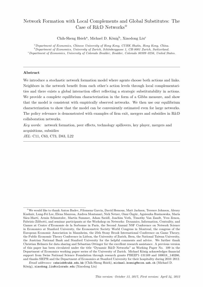
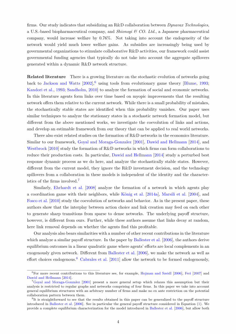
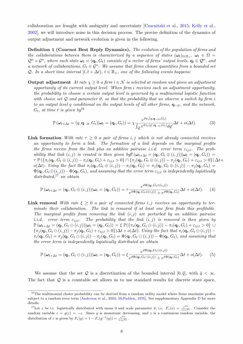
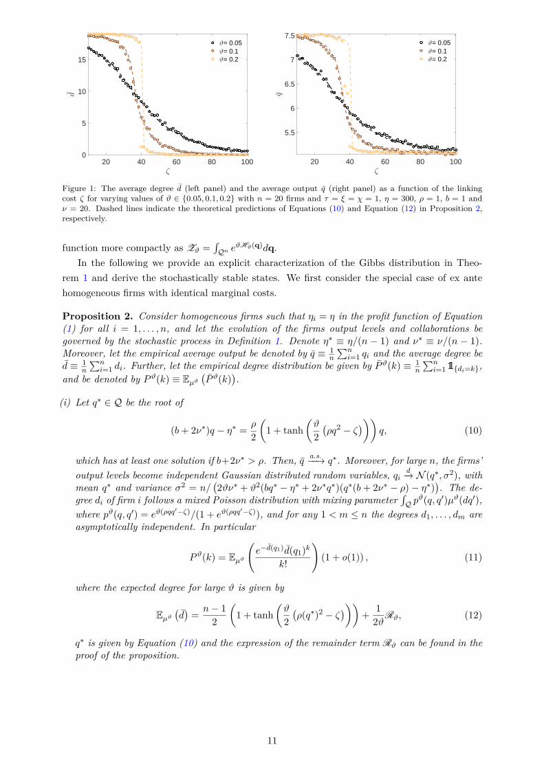
Figure 1: The average degree d (left panel) and the average output q (right panel) as a function of the linkingcost ζ for varying values of ϑ ∈ 0.05, 0.1, 0.2 with n = 20 firms and τ = ξ = χ = 1, η = 300, ρ = 1, b = 1 andν = 20. Dashed lines indicate the theoretical predictions of Equations (10) and Equation (12) in Proposition 2,respectively.
function more compactly as Zϑ =∫Qn e
ϑHϑ(q)dq.In the following we provide an explicit characterization of the Gibbs distribution in Theo-
rem 1 and derive the stochastically stable states. We first consider the special case of ex antehomogeneous firms with identical marginal costs.
Proposition 2. Consider homogeneous firms such that ηi = η in the profit function of Equation(1) for all i = 1, . . . , n, and let the evolution of the firms output levels and collaborations begoverned by the stochastic process in Definition 1. Denote η∗ ≡ η/(n − 1) and ν∗ ≡ ν/(n − 1).Moreover, let the empirical average output be denoted by q ≡ 1
n
∑ni=1 qi and the average degree be
d ≡ 1n
∑ni=1 di. Further, let the empirical degree distribution be given by P ϑ(k) ≡ 1
n
∑ni=1 1di=k,
and be denoted by P ϑ(k) ≡ Eµϑ(P ϑ(k)
).
(i) Let q∗ ∈ Q be the root of
(b+ 2ν∗)q − η∗ =ρ
2
(1 + tanh
(ϑ
2
(ρq2 − ζ
)))q, (10)
which has at least one solution if b+2ν∗ > ρ. Then, q a.s.−−→ q∗. Moreover, for large n, the firms’output levels become independent Gaussian distributed random variables, qi
d−→ N (q∗, σ2), withmean q∗ and variance σ2 = n/
(2ϑν∗ + ϑ2(bq∗ − η∗ + 2ν∗q∗)(q∗(b+ 2ν∗ − ρ)− η∗)
). The de-
gree di of firm i follows a mixed Poisson distribution with mixing parameter∫Q p
ϑ(q, q′)µϑ(dq′),where pϑ(q, q′) = eϑ(ρqq
′−ζ)/(1 + eϑ(ρqq′−ζ)), and for any 1 < m ≤ n the degrees d1, . . . , dm are
asymptotically independent. In particular
P ϑ(k) = Eµϑ
(e−d(q1)d(q1)
k
k!
)(1 + o(1)) , (11)
where the expected degree for large ϑ is given by
Eµϑ(d)=n− 1
2
(1 + tanh
(ϑ
2
(ρ(q∗)2 − ζ
)))+
1
2ϑRϑ, (12)
q∗ is given by Equation (10) and the expression of the remainder term Rϑ can be found in theproof of the proposition.
11
ρ
b
high equi l ibrium
multip l e equi l ibria
low equi l ibrium
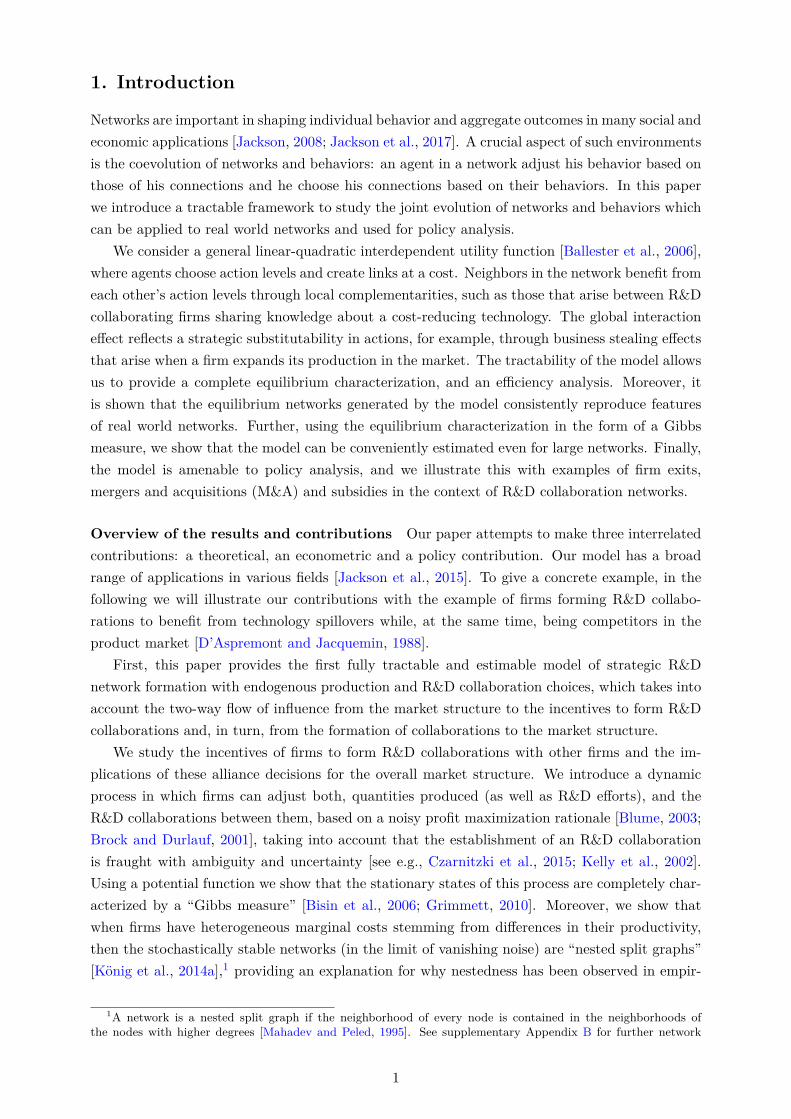
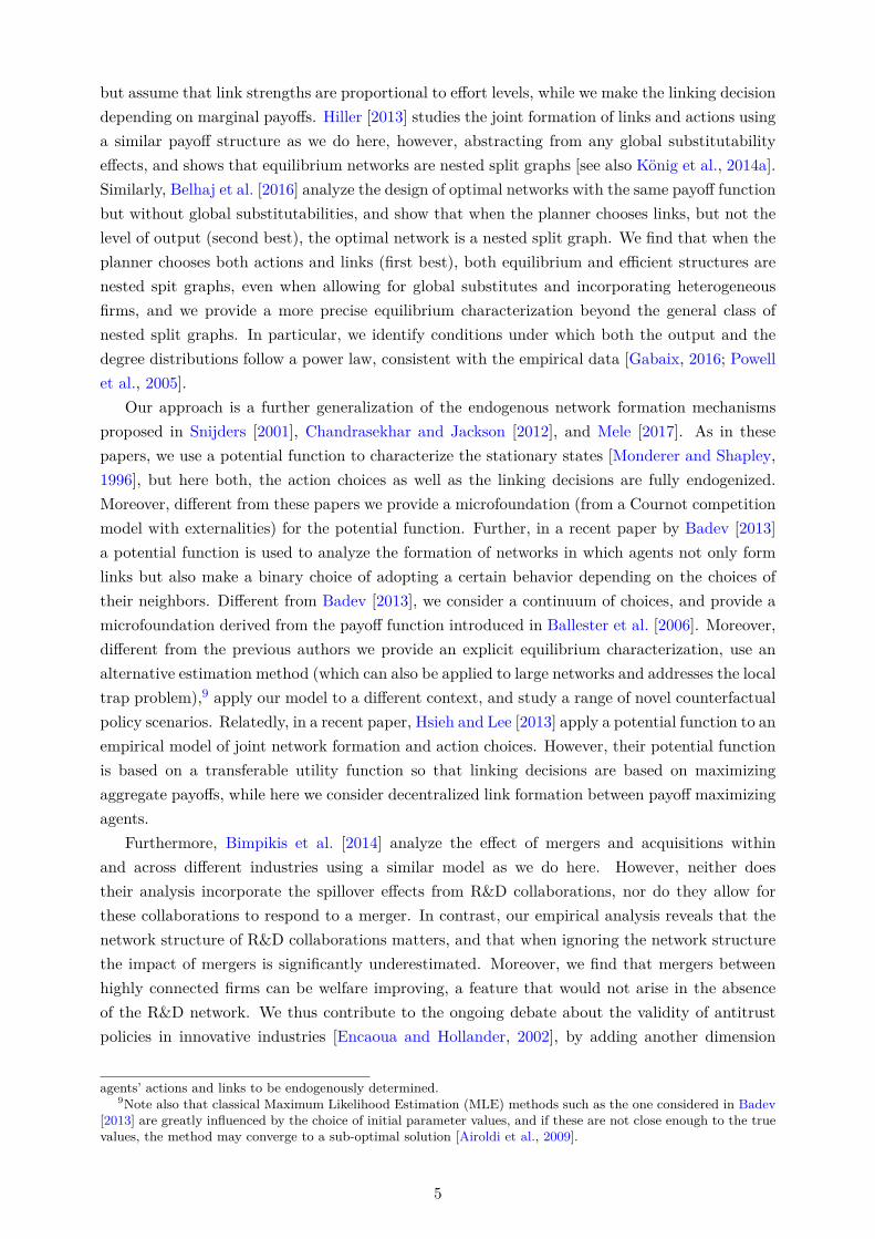
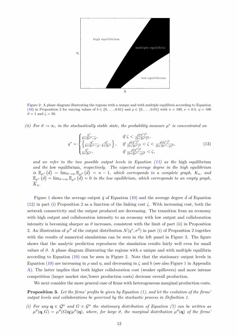
Figure 2: A phase diagram illustrating the regions with a unique and with multiple equilibria according to Equation(10) in Proposition 2 for varying values of b ∈ 0, . . . , 0.01 and ρ ∈ 0, . . . , 0.01 with n = 100, ν = 0.5, η = 100ϑ = 1 and ζ = 50.
(ii) For ϑ→ ∞, in the stochastically stable state, the probability measure µ∗ is concentrated on
q∗ =
η∗
b+2ν∗−ρ , if ζ < ρ(η∗)2
(b+2ν∗)2 ,η∗
b+2ν∗−ρ ,η∗
b+2ν∗
, if ρ(η∗)2
(b+2ν∗)2 < ζ < ρ(η∗)2
(b+2ν∗−ρ)2 ,
η∗
b+2ν∗ , if ρ(η∗)2
(b+2ν∗−ρ)2 < ζ,
(13)
and we refer to the two possible output levels in Equation (13) as the high equilibriumand the low equilibrium, respectively. The expected average degree in the high equilibriumis Eµ∗
(d)
= limϑ→∞ Eµϑ(d)
= n − 1, which corresponds to a complete graph, Kn, andEµ∗
(d)= limϑ→∞ Eµϑ
(d)= 0 in the low equilibrium, which corresponds to an empty graph,
Kn.
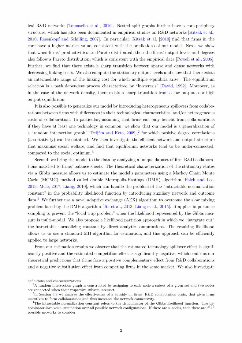
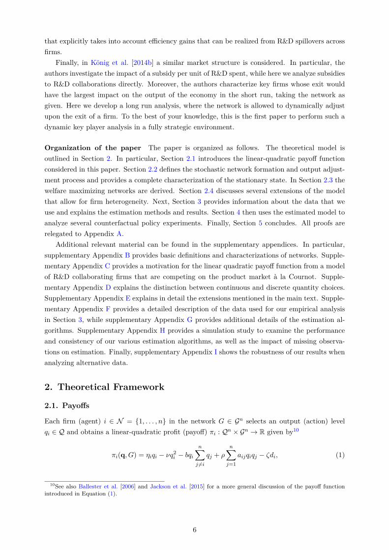
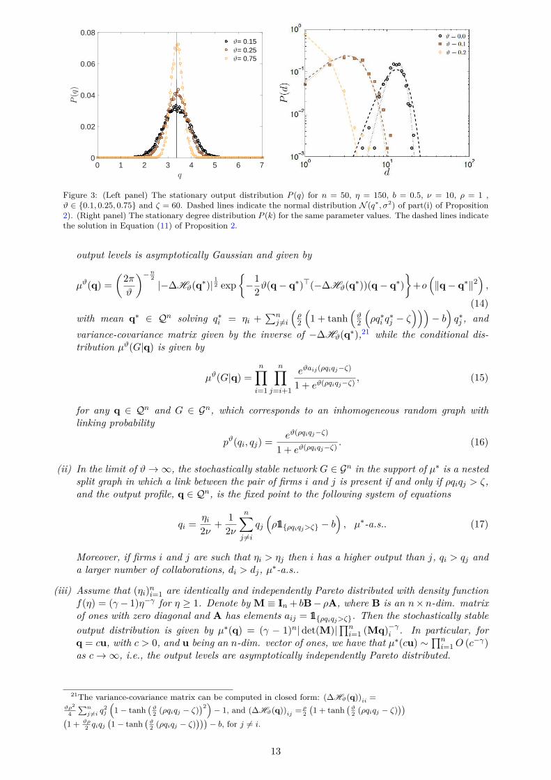
Figure 1 shows the average output q of Equation (10) and the average degree d of Equation(12) in part (i) Proposition 2 as a function of the linking cost ζ. With increasing cost, both thenetwork connectivity and the output produced are decreasing. The transition from an economywith high output and collaboration intensity to an economy with low output and collaborationintensity is becoming sharper as ϑ increases, consistent with the limit of part (ii) in Proposition2. An illustration of µϑ of the output distribution N (q∗, σ2) in part (i) of Proposition 2 togetherwith the results of numerical simulations can be seen in the left panel in Figure 3. The figureshows that the analytic prediction reproduces the simulation results fairly well even for smallvalues of ϑ. A phase diagram illustrating the regions with a unique and with multiple equilibriaaccording to Equation (10) can be seen in Figure 2. Note that the stationary output levels inEquation (10) are increasing in ρ and η, and decreasing in ζ and b (see also Figure 1 in AppendixA). The latter implies that both higher collaboration cost (weaker spillovers) and more intensecompetition (larger market size/lower production costs) decrease overall production.
We next consider the more general case of firms with heterogeneous marginal production costs.
Proposition 3. Let the firms’ profits be given by Equation (1), and let the evolution of the firms’output levels and collaborations be governed by the stochastic process in Definition 1.
(i) For any q ∈ Qn and G ∈ Gn the stationary distribution of Equation (7) can be written asµϑ(q, G) = µϑ(G|q)µϑ(q), where, for large ϑ, the marginal distribution µϑ(q) of the firms’
12
0 1 2 3 4 5 6 7q
0
0.02
0.04
0.06
0.08
P(q)
ϑ= 0.15ϑ= 0.25ϑ= 0.75
Figure 3: (Left panel) The stationary output distribution P (q) for n = 50, η = 150, b = 0.5, ν = 10, ρ = 1 ,ϑ ∈ 0.1, 0.25, 0.75 and ζ = 60. Dashed lines indicate the normal distribution N (q∗, σ2) of part(i) of Proposition2). (Right panel) The stationary degree distribution P (k) for the same parameter values. The dashed lines indicatethe solution in Equation (11) of Proposition 2.
output levels is asymptotically Gaussian and given by
µϑ(q) =
(2π
ϑ
)−n2
|−∆Hϑ(q∗)|
12 exp
−1
2ϑ(q− q∗)⊤(−∆Hϑ(q
∗))(q− q∗)
+o(∥q− q∗∥2
),
(14)with mean q∗ ∈ Qn solving q∗i = ηi +
∑nj =i
(ρ2
(1 + tanh
(ϑ2
(ρq∗i q
∗j − ζ
)))− b)q∗j , and
variance-covariance matrix given by the inverse of −∆Hϑ(q∗),21 while the conditional dis-
tribution µϑ(G|q) is given by
µϑ(G|q) =n∏i=1
n∏j=i+1
eϑaij(ρqiqj−ζ)
1 + eϑ(ρqiqj−ζ), (15)
for any q ∈ Qn and G ∈ Gn, which corresponds to an inhomogeneous random graph withlinking probability
pϑ(qi, qj) =eϑ(ρqiqj−ζ)
1 + eϑ(ρqiqj−ζ). (16)
(ii) In the limit of ϑ→ ∞, the stochastically stable network G ∈ Gn in the support of µ∗ is a nestedsplit graph in which a link between the pair of firms i and j is present if and only if ρqiqj > ζ,and the output profile, q ∈ Qn, is the fixed point to the following system of equations
qi =ηi2ν
+1
2ν
n∑j =i
qj
(ρ1ρqiqj>ζ − b
), µ∗-a.s.. (17)
Moreover, if firms i and j are such that ηi > ηj then i has a higher output than j, qi > qj anda larger number of collaborations, di > dj, µ∗-a.s..
(iii) Assume that (ηi)ni=1 are identically and independently Pareto distributed with density functionf(η) = (γ− 1)η−γ for η ≥ 1. Denote by M ≡ In+ bB− ρA, where B is an n×n-dim. matrixof ones with zero diagonal and A has elements aij = 1ρqiqj>ζ. Then the stochastically stableoutput distribution is given by µ∗(q) = (γ − 1)n| det(M)|
∏ni=1 (Mq)−γi . In particular, for
q = cu, with c > 0, and u being an n-dim. vector of ones, we have that µ∗(cu) ∼∏ni=1O (c−γ)
as c→ ∞, i.e., the output levels are asymptotically independently Pareto distributed.
21The variance-covariance matrix can be computed in closed form: (∆Hϑ(q))ii =ϑρ2
4
∑nj =i q
2j
(1− tanh
(ϑ2(ρqiqj − ζ)
)2)− 1, and (∆Hϑ(q))ij = ρ2
(1 + tanh
(ϑ2(ρqiqj − ζ)
))(1 + ϑρ
2qiqj
(1− tanh
(ϑ2(ρqiqj − ζ)
)))− b, for j = i.
13
A
2 4 6 8 10i
2
4
6
8
10
j
A
2 4 6 8 10i
2
4
6
8
10
j
A
2 4 6 8 10i
2
4
6
8
10
j
Figure 4: The (stepwise) adjacency matrix A = (aij)1≤i,j≤n, characteristic of a nested split graph, with elementsgiven by aij = 1
qiqj>ζρ
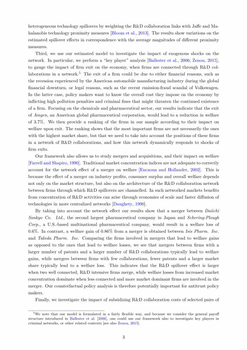
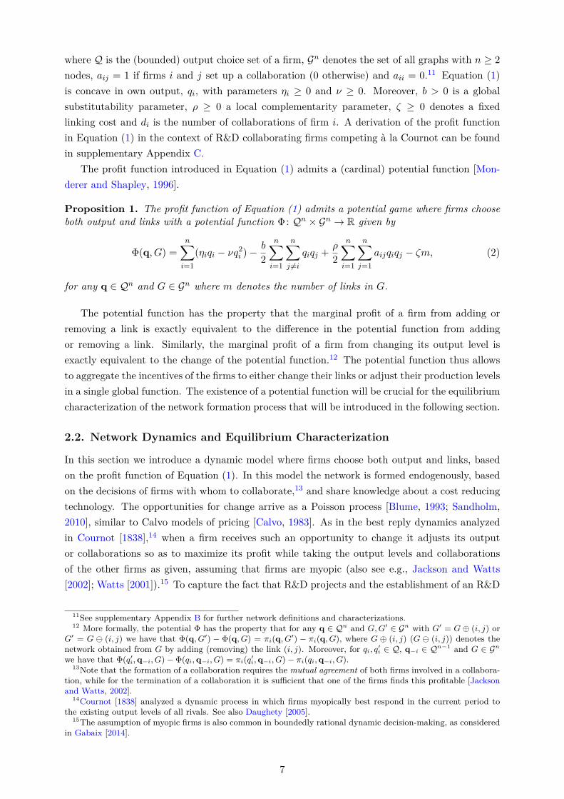
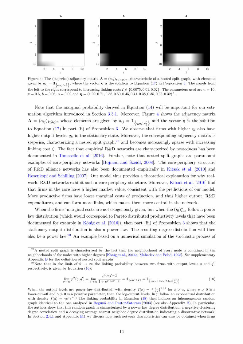
, where the vector q is the solution to Equation (17) in Proposition 3. The panels fromthe left to the right correspond to increasing linking costs ζ ∈ 0.0075, 0.01, 0.02. The parameters used are n = 10,ν = 0.5, b = 0.06, ρ = 0.02 and η = (1.00, 0.71, 0.58, 0.50, 0.45, 0.41, 0.38, 0.35, 0.33, 0.32)⊤.
Note that the marginal probability derived in Equation (14) will be important for our esti-mation algorithm introduced in Section 3.3.1. Moreover, Figure 4 shows the adjacency matrixA = (aij)1≤i,j,n whose elements are given by aij = 1
qiqj>ζρ
and the vector q is the solution
to Equation (17) in part (ii) of Proposition 3. We observe that firms with higher ηi also havehigher output levels, qi, in the stationary state. Moreover, the corresponding adjacency matrix isstepwise, characterizing a nested split graph,22 and becomes increasingly sparse with increasinglinking cost ζ. The fact that empirical R&D networks are characterized by nestedness has beendocumented in Tomasello et al. [2016]. Further, note that nested split graphs are paramountexamples of core-periphery networks [Hojman and Szeidl, 2008]. The core-periphery structureof R&D alliance networks has also been documented empirically in Kitsak et al. [2010] andRosenkopf and Schilling [2007]. Our model thus provides a theoretical explanation for why real-world R&D networks exhibit such a core-periphery structure. Moreover, Kitsak et al. [2010] findthat firms in the core have a higher market value, consistent with the predictions of our model.More productive firms have lower marginal costs of production, and thus higher output, R&Dexpenditures, and can form more links, which makes them more central in the network.
When the firms’ marginal costs are not exogenously given, but when the (ηi)ni=1 follow a power
law distribution (which would correspond to Pareto distributed productivity levels that have beendocumented for example in König et al. [2016]), then part (iii) of Proposition 3 shows that thestationary output distribution is also a power law. The resulting degree distribution will thenalso be a power law.23 An example based on a numerical simulation of the stochastic process of
22A nested split graph is characterized by the fact that the neighborhood of every node is contained in theneighborhoods of the nodes with higher degrees [König et al., 2014a; Mahadev and Peled, 1995]. See supplementaryAppendix B for the definition of nested split graphs.
23Note that in the limit of ϑ → ∞ the linking probability between two firms with output levels q and q′,respectively, is given by Equation (16):
limϑ→∞
pϑ(q, q′) = limϑ→∞
eϑ(ρqq′−ζ)
1 + eϑ(ρqq′−ζ)= 1ρqq′>ζ = 1
log q+log q′>log(
ζρ
). (18)
When the output levels are power law distributed, with density f(x) = γc
(cx
)γ+1 for x > c, where c > 0 is alower-cut-off and γ > 0 is a positive parameter, then the log-ouptut levels, ln q, follow an exponential distributionwith density f(y) = γcγe−γy.The linking probability in Equation (18) then induces an inhomogenous randomgraph identical to the one analyzed in Boguná and Pastor-Satorras [2003] (see also Appendix B). In particular,the authors show that this random graph is characterized by a power law degree distribution, a negative clusteringdegree correlation and a decaying average nearest neighbor degree distribution indicating a dissortative network.In Section 2.4.1 and Appendix E.1 we discuss how such network characteristics can also be obtained when firms
14
100 101
η
10-3
10-2
10-1
100
P(η)
100 101 102
q
100
P(q)
100 101 102
d
100
P(d)
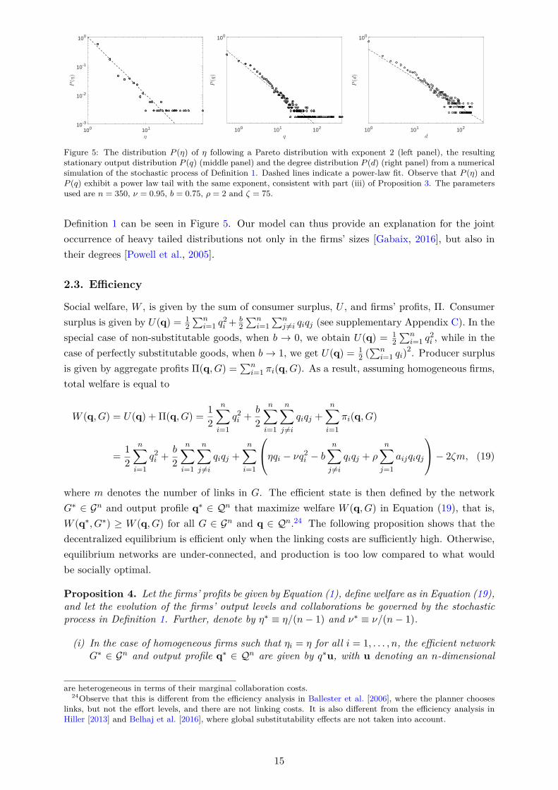
Figure 5: The distribution P (η) of η following a Pareto distribution with exponent 2 (left panel), the resultingstationary output distribution P (q) (middle panel) and the degree distribution P (d) (right panel) from a numericalsimulation of the stochastic process of Definition 1. Dashed lines indicate a power-law fit. Observe that P (η) andP (q) exhibit a power law tail with the same exponent, consistent with part (iii) of Proposition 3. The parametersused are n = 350, ν = 0.95, b = 0.75, ρ = 2 and ζ = 75.
Definition 1 can be seen in Figure 5. Our model can thus provide an explanation for the jointoccurrence of heavy tailed distributions not only in the firms’ sizes [Gabaix, 2016], but also intheir degrees [Powell et al., 2005].
2.3. Efficiency
Social welfare, W , is given by the sum of consumer surplus, U , and firms’ profits, Π. Consumersurplus is given by U(q) = 1
2
∑ni=1 q
2i +
b2
∑ni=1
∑nj =i qiqj (see supplementary Appendix C). In the
special case of non-substitutable goods, when b → 0, we obtain U(q) = 12
∑ni=1 q
2i , while in the
case of perfectly substitutable goods, when b→ 1, we get U(q) = 12 (∑n
i=1 qi)2. Producer surplus
is given by aggregate profits Π(q, G) =∑n
i=1 πi(q, G). As a result, assuming homogeneous firms,total welfare is equal to
W (q, G) = U(q) + Π(q, G) =1
2
n∑i=1
q2i +b
2
n∑i=1
n∑j =i
qiqj +n∑i=1
πi(q, G)
=1
2
n∑i=1
q2i +b
2
n∑i=1
n∑j =i
qiqj +n∑i=1
ηqi − νq2i − bn∑j =i
qiqj + ρn∑j=1
aijqiqj
− 2ζm, (19)
where m denotes the number of links in G. The efficient state is then defined by the networkG∗ ∈ Gn and output profile q∗ ∈ Qn that maximize welfare W (q, G) in Equation (19), that is,W (q∗, G∗) ≥ W (q, G) for all G ∈ Gn and q ∈ Qn.24 The following proposition shows that thedecentralized equilibrium is efficient only when the linking costs are sufficiently high. Otherwise,equilibrium networks are under-connected, and production is too low compared to what wouldbe socially optimal.
Proposition 4. Let the firms’ profits be given by Equation (1), define welfare as in Equation (19),and let the evolution of the firms’ output levels and collaborations be governed by the stochasticprocess in Definition 1. Further, denote by η∗ ≡ η/(n− 1) and ν∗ ≡ ν/(n− 1).
(i) In the case of homogeneous firms such that ηi = η for all i = 1, . . . , n, the efficient networkG∗ ∈ Gn and output profile q∗ ∈ Qn are given by q∗u, with u denoting an n-dimensional
are heterogeneous in terms of their marginal collaboration costs.24Observe that this is different from the efficiency analysis in Ballester et al. [2006], where the planner chooses
links, but not the effort levels, and there are not linking costs. It is also different from the efficiency analysis inHiller [2013] and Belhaj et al. [2016], where global substitutability effects are not taken into account.
15
20 40 60 80 100ζ
1.5
2
2.5
3
3.5
4
W(q,G
)
×104
Kn Kn
ζ∗
ϑ= 0.05ϑ= 0.1ϑ= 0.2
20 40 60 80 100ζ
0.5
0.6
0.7
0.8
0.9
W(q,G
)/W
(q∗,G
∗)
ζ∗
ϑ= 0.05ϑ= 0.1ϑ= 0.2
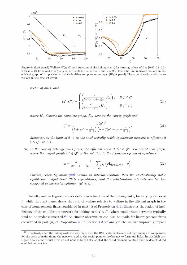
Figure 6: (Left panel) Welfare W (q, G) as a function of the linking cost ζ for varying values of ϑ ∈ 0.05, 0.1, 0.2with n = 20 firms and τ = ξ = χ = 1, η = 300, ρ = 1, b = 1 and ν = 20. The solid line indicates welfare in theefficient graph of Proposition 4 (which is either complete or empty). (Right panel) The ratio of welfare relative towelfare in the efficient graph.
vector of ones, and
(q∗, G∗) =
(
η∗
b+2(ν∗−ρ)− 1n−1
,Kn
), if ζ ≤ ζ∗,(
η∗
b+2ν∗− 1n−1
,Kn
), if ζ∗ < ζ,
(20)
where Kn denotes the complete graph, Kn denotes the empty graph and
ζ∗ =ρ (η∗)2(
b+ 2ν∗ − 1n−1
)(b+ 2(ν∗ − ρ)− 1
n−1
) . (21)
Moreover, in the limit of ϑ→ ∞ the stochastically stable equilibrium network is efficient ifζ > ζ∗, µ∗-a.s..
(ii) In the case of heterogeneous firms, the efficient network G∗ ∈ Gn is a nested split graph,where the output profile q∗ ∈ Qn is the solution to the following system of equations
qi =ηi
2ν − 1+
1
2ν − 1
n∑j =i
qj
(ρ1ρqiqj>ζ − b
). (22)
Further, when Equation (22) admits an interior solution, then the stochastically stableequilibrium output (and R&D expenditures) and the collaboration intensity are too lowcompared to the social optimum (µ∗-a.s.).
The left panel in Figure 6 shows welfare as a function of the linking cost ζ for varying values ofϑ, while the right panel shows the ratio of welfare relative to welfare in the efficient graph in thecase of homogeneous firms considered in part (i) of Proposition 4. It illustrates the region of inef-ficiency of the equilibrium network for linking costs ζ < ζ∗, where equilibrium networks typicallytend to be under-connected.25 As similar observation can also be made for heterogeneous firmsconsidered in part (ii) of Proposition 4. In Section 4.3 we analyze the welfare improving impact
25In contrast, when the linking costs are very high, then the R&D externalities are not high enough to compensatefor the costs of maintaining the network, and so the social planner prefers not to form any links. In this high costregion also the individual firms do not want to form links, so that the social planners solution and the decentralizedequilibrium coincide.
16
of a subsidy on firms’ R&D collaboration costs, that incentivises firms to form collaborations andthus increases the network connectivity.
2.4. Extensions
The model presented so far can be extended in a number of different directions that account forfirm heterogeneity, which are summarized below and described in greater detail in supplementaryAppendix E.
2.4.1. Heterogeneous Collaboration Costs
We can extend the model by assuming that firms with higher productivity incur lower collabo-ration costs (see also supplementary Appendix E.1). One can show that a similar equilibriumcharacterization using a Gibbs measure as in Theorem 1 is possible. Moreover, in the specialcase that the productivity is power law distributed, one can show that the degree distributionalso follows a power law distribution (see Proposition 5),26 consistent with previous empiricalstudies of R&D networks [see e.g., Powell et al., 2005], together with other empirically relevantcorrelations (see Propositions 6 and 7).27
2.4.2. Heterogeneous Technology Spillovers
We can further extend the model by assuming that there are heterogeneous spillovers betweencollaborating firms depending on their technology portfolios [Griffith et al., 2003] (see also sup-plementary Appendix E.2). For example, assume that firms can only benefit from collaborationsif they have at least one technology in common. Then one can show that our model is a general-ization of a “random intersection graph” [Deijfen and Kets, 2009] (see supplementary AppendixB) for which positive degree correlations can be obtained (i.e., “assortativity”, see Proposition8).
The above extensions show that our model is capable of generating networks with propertiesthat can be observed in real world networks, such as power law degree distributions and variousdegree correlations, once we introduce firm heterogeneity. This counteracts general criticismof (simple variants of) exponential random graphs, which often have difficulties in generatingnetworks with empirically relevant characteristics [Chandrasekhar and Jackson, 2012].
26In particular, assume that the productivity s are distributed as a power law s−γ with exponent γ. Then on canshow that the asymptotic degree distribution is also power law distributed, P (k) ∼ k
− γγ−1 , with exponent γ
γ−1.
27We note that also other statistics such as the clustering degree distribution can be computed. See supplementaryAppendix E.2 for further details. In particular, under the assumptions of a power law productivity distribution,we can generate two-vertex and three-vertex degree correlations, such as a decreasing average nearest neighborconnectivity, knn(d), indicating a dissortative network, as well as a decreasing clustering degree distribution, C(d),with the degree d.
17
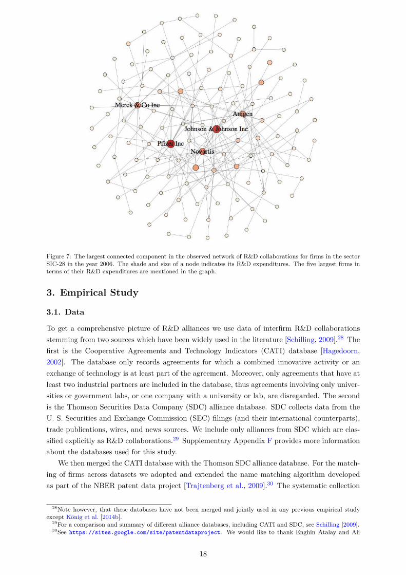
Figure 7: The largest connected component in the observed network of R&D collaborations for firms in the sectorSIC-28 in the year 2006. The shade and size of a node indicates its R&D expenditures. The five largest firms interms of their R&D expenditures are mentioned in the graph.
3. Empirical Study
3.1. Data
To get a comprehensive picture of R&D alliances we use data of interfirm R&D collaborationsstemming from two sources which have been widely used in the literature [Schilling, 2009].28 Thefirst is the Cooperative Agreements and Technology Indicators (CATI) database [Hagedoorn,2002]. The database only records agreements for which a combined innovative activity or anexchange of technology is at least part of the agreement. Moreover, only agreements that have atleast two industrial partners are included in the database, thus agreements involving only univer-sities or government labs, or one company with a university or lab, are disregarded. The secondis the Thomson Securities Data Company (SDC) alliance database. SDC collects data from theU. S. Securities and Exchange Commission (SEC) filings (and their international counterparts),trade publications, wires, and news sources. We include only alliances from SDC which are clas-sified explicitly as R&D collaborations.29 Supplementary Appendix F provides more informationabout the databases used for this study.
We then merged the CATI database with the Thomson SDC alliance database. For the match-ing of firms across datasets we adopted and extended the name matching algorithm developedas part of the NBER patent data project [Trajtenberg et al., 2009].30 The systematic collection
28Note however, that these databases have not been merged and jointly used in any previous empirical studyexcept König et al. [2014b].
29For a comparison and summary of different alliance databases, including CATI and SDC, see Schilling [2009].30See https://sites.google.com/site/patentdataproject. We would like to thank Enghin Atalay and Ali
18
of inter-firm alliances in CATI started in 1987 and ended in 2006. As the CATI database onlyincludes collaborations up to the year 2006, we take this year as the base year for our empiricalanalysis. We then construct the R&D alliance network by assuming that an alliance lasts for 5years [similar to e.g., Rosenkopf and Padula, 2008]. The corresponding entry in the adjacencymatrix between two firms is coded as one if an alliance between them exists during this period,and zero otherwise. An illustration of the observed R&D network can be seen in Figure 3.1.
The combined CATI-SDC database only provides the names for each firm in an alliance.We therefore matched the firms’ names in the CATI-SDC database with the firms’ names inStandard & Poor’s Compustat U.S. and Global Fundamentals databases, as well as Bureau vanDijk’s Orbis database, to obtain information about their balance sheets and income statements[see e.g., Bloom et al., 2013]. For the purpose of matching firms across databases, we employ theabove mentioned name matching algorithm. We could match roughly 25% of the firms in thealliance data for which balance sheet information was available.31 From our match between thefirms’ names in the alliance database and the firms’ names in the Compustat and Orbis databases,we obtained a firm’s R&D expenditures, sales, employment, primary industry code, and location.We computed firm’s labor productivity as sales relative to the number of employees.32,33
To be consistent with our theoretical model (see Section 2 and supplementary Appendix C)where a firm’s output is proportional to its R&D effort, we use the logarithm of firm’s R&D expen-diture to measure its R&D effort and thus the output. We further identify the patent portfoliosof the firms in our dataset using the EPO Worldwide Patent Statistical Database (PATSTAT)[Jaffe and Trajtenberg, 2002] (see also supplementary Appendix F.4). We only consider grantedpatents (or successful patents), as opposed to patents applied for, as they are the main drivers ofrevenue derived from R&D [Copeland and Fixler, 2012]. We obtained matches for roughly 30% ofthe firms in the data. The technology classes were identified using the main international patentclassification (IPC) numbers at the 4-digit level. After removing firm observations with missingvalues on sales, employment, and R&D expenditures, we regard the remaining 1,201 firms (with428 R&D collaborations) as the full sample for our analysis.34 Some descriptive statistics of thisfull sample are shown in the first row of Table 1.
The size of the sample including all sectors is somewhat too large to make some of the esti-mation methods that we will introduce below become computationally infeasible (in particularthe exchange algorithm and adaptive exchange algorithm in Sections 3.3.2 and 3.3.3),35 we fur-
Hortacsu for sharing their name matching algorithm with us.31Note that for many small private firms no balance sheet information is available, and hence these firms could
not be matched by our algorithm. We therefore typically exclude smaller private firms from our analysis, but thisis inevitable if one is going to use market value data. Nevertheless, R&D is mostly concentrated in publicly listedfirms, which cover most of the R&D activities in the economy [see e.g., Bloom et al., 2013], and these firms aretypically included in our sample.
32Labor productivity can vary across firms in different industries, in particular when industries differ greatly intheir labor intensity of production. However, these difference should have a limited effect as we include industryfixed effects.
33We find that our results remain robust when using output-labor productivity instead of revenue-labor produc-tivity. The results can be obtained upon request from the authors.
34To understand the impact of missing observations due to incomplete matching between databases, we conducta Monte Carlo simulation study in supplementary Appendix H.
35See Section 3.3 and supplementary Appendix H for a more detailed discussion of the various estimation pro-cedures that we introduce in this paper. Further, note that the restriction to small sample sizes does not apply tothe likelihood partition approach introduced in Section 3.3.1, for which we can use the full sample to estimate theparameters of the model. We find, however, that the estimation results are similar, irrespective of whether we useonly a subsample of the data or the whole sample. Compared to several existing studies, [e.g. Badev, 2013; Hsieh
19
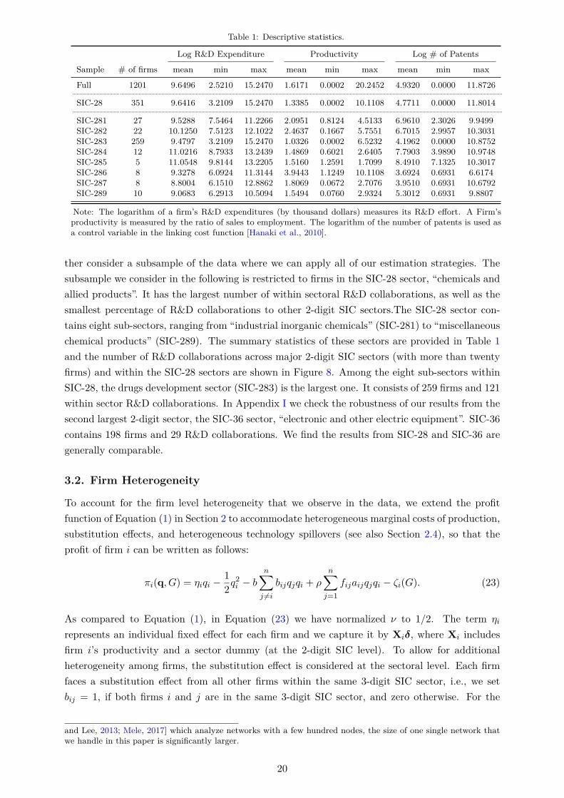
Table 1: Descriptive statistics.
Log R&D Expenditure Productivity Log # of Patents
Sample # of firms mean min max mean min max mean min max
Full 1201 9.6496 2.5210 15.2470 1.6171 0.0002 20.2452 4.9320 0.0000 11.8726
SIC-28 351 9.6416 3.2109 15.2470 1.3385 0.0002 10.1108 4.7711 0.0000 11.8014
SIC-281 27 9.5288 7.5464 11.2266 2.0951 0.8124 4.5133 6.9610 2.3026 9.9499SIC-282 22 10.1250 7.5123 12.1022 2.4637 0.1667 5.7551 6.7015 2.9957 10.3031SIC-283 259 9.4797 3.2109 15.2470 1.0326 0.0002 6.5232 4.1962 0.0000 10.8752SIC-284 12 11.0216 8.7933 13.2439 1.4869 0.6021 2.6405 7.7903 3.9890 10.9748SIC-285 5 11.0548 9.8144 13.2205 1.5160 1.2591 1.7099 8.4910 7.1325 10.3017SIC-286 8 9.3278 6.0924 11.3144 3.9443 1.1249 10.1108 3.6924 0.6931 6.6174SIC-287 8 8.8004 6.1510 12.8862 1.8069 0.0672 2.7076 3.9510 0.6931 10.6792SIC-289 10 9.0683 6.2913 10.5094 1.5494 0.0760 2.9324 5.3012 0.6931 9.8807
Note: The logarithm of a firm’s R&D expenditures (by thousand dollars) measures its R&D effort. A Firm’sproductivity is measured by the ratio of sales to employment. The logarithm of the number of patents is used asa control variable in the linking cost function [Hanaki et al., 2010].
ther consider a subsample of the data where we can apply all of our estimation strategies. Thesubsample we consider in the following is restricted to firms in the SIC-28 sector, “chemicals andallied products”. It has the largest number of within sectoral R&D collaborations, as well as thesmallest percentage of R&D collaborations to other 2-digit SIC sectors.The SIC-28 sector con-tains eight sub-sectors, ranging from “industrial inorganic chemicals” (SIC-281) to “miscellaneouschemical products” (SIC-289). The summary statistics of these sectors are provided in Table 1and the number of R&D collaborations across major 2-digit SIC sectors (with more than twentyfirms) and within the SIC-28 sectors are shown in Figure 8. Among the eight sub-sectors withinSIC-28, the drugs development sector (SIC-283) is the largest one. It consists of 259 firms and 121within sector R&D collaborations. In Appendix I we check the robustness of our results from thesecond largest 2-digit sector, the SIC-36 sector, “electronic and other electric equipment”. SIC-36contains 198 firms and 29 R&D collaborations. We find the results from SIC-28 and SIC-36 aregenerally comparable.
3.2. Firm Heterogeneity
To account for the firm level heterogeneity that we observe in the data, we extend the profitfunction of Equation (1) in Section 2 to accommodate heterogeneous marginal costs of production,substitution effects, and heterogeneous technology spillovers (see also Section 2.4), so that theprofit of firm i can be written as follows:
πi(q, G) = ηiqi −1
2q2i − b
n∑j =i
bijqjqi + ρ
n∑j=1
fijaijqjqi − ζi(G). (23)
As compared to Equation (1), in Equation (23) we have normalized ν to 1/2. The term ηi
represents an individual fixed effect for each firm and we capture it by Xiδ, where Xi includesfirm i’s productivity and a sector dummy (at the 2-digit SIC level). To allow for additionalheterogeneity among firms, the substitution effect is considered at the sectoral level. Each firmfaces a substitution effect from all other firms within the same 3-digit SIC sector, i.e., we setbij = 1, if both firms i and j are in the same 3-digit SIC sector, and zero otherwise. For the
and Lee, 2013; Mele, 2017] which analyze networks with a few hundred nodes, the size of one single network thatwe handle in this paper is significantly larger.
20
B
i
j
B
i
j
20 33 87 37 73 35 38 36 28
20 0 0 1 1 0 0 1 0 333 0 1 0 4 0 2 1 3 187 1 0 0 0 1 2 4 3 1437 1 4 0 17 5 2 7 2 173 0 0 1 5 4 17 7 17 635 0 2 2 2 17 9 5 26 238 1 1 4 7 7 5 6 13 2536 0 3 3 2 17 26 13 29 328 3 1 14 1 6 2 25 3 141
281 282 283 284 285 286 287 289
281 1 2 13 0 0 0 0 0282 2 1 1 0 0 0 0 0283 13 1 121 0 2 0 0 0284 0 0 0 0 0 0 0 0285 0 0 2 0 0 0 0 0286 0 0 0 0 0 0 0 0287 0 0 0 0 0 0 0 0289 0 0 0 0 0 0 0 0
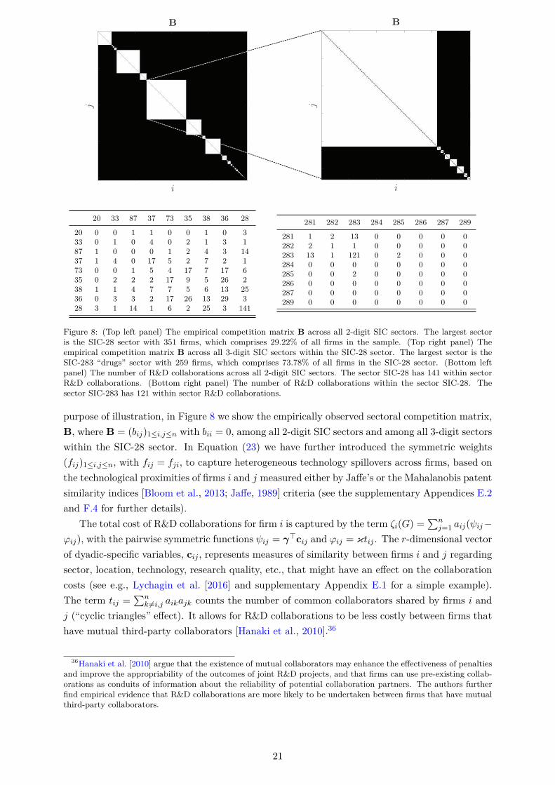
Figure 8: (Top left panel) The empirical competition matrix B across all 2-digit SIC sectors. The largest sectoris the SIC-28 sector with 351 firms, which comprises 29.22% of all firms in the sample. (Top right panel) Theempirical competition matrix B across all 3-digit SIC sectors within the SIC-28 sector. The largest sector is theSIC-283 “drugs” sector with 259 firms, which comprises 73.78% of all firms in the SIC-28 sector. (Bottom leftpanel) The number of R&D collaborations across all 2-digit SIC sectors. The sector SIC-28 has 141 within sectorR&D collaborations. (Bottom right panel) The number of R&D collaborations within the sector SIC-28. Thesector SIC-283 has 121 within sector R&D collaborations.
purpose of illustration, in Figure 8 we show the empirically observed sectoral competition matrix,B, where B = (bij)1≤i,j≤n with bii = 0, among all 2-digit SIC sectors and among all 3-digit sectorswithin the SIC-28 sector. In Equation (23) we have further introduced the symmetric weights(fij)1≤i,j≤n, with fij = fji, to capture heterogeneous technology spillovers across firms, based onthe technological proximities of firms i and j measured either by Jaffe’s or the Mahalanobis patentsimilarity indices [Bloom et al., 2013; Jaffe, 1989] criteria (see the supplementary Appendices E.2and F.4 for further details).
The total cost of R&D collaborations for firm i is captured by the term ζi(G) =∑n
j=1 aij(ψij−φij), with the pairwise symmetric functions ψij = γ⊤cij and φij = κtij . The r-dimensional vectorof dyadic-specific variables, cij , represents measures of similarity between firms i and j regardingsector, location, technology, research quality, etc., that might have an effect on the collaborationcosts (see e.g., Lychagin et al. [2016] and supplementary Appendix E.1 for a simple example).The term tij =
∑nk =i,j aikajk counts the number of common collaborators shared by firms i and
j (“cyclic triangles” effect). It allows for R&D collaborations to be less costly between firms thathave mutual third-party collaborators [Hanaki et al., 2010].36
36Hanaki et al. [2010] argue that the existence of mutual collaborators may enhance the effectiveness of penaltiesand improve the appropriability of the outcomes of joint R&D projects, and that firms can use pre-existing collab-orations as conduits of information about the reliability of potential collaboration partners. The authors furtherfind empirical evidence that R&D collaborations are more likely to be undertaken between firms that have mutualthird-party collaborators.
21
The potential function Φ: Rn+ × Gn → R corresponding to Equation (23) is given by12
Φ(q, G) =n∑i=1
(ηiqi −
1
2q2i
)− b2
n∑i=1
n∑j =i
bijqiqj+ρ
2
n∑i=1
n∑j =i
fijaijqiqj−1
2
n∑i=1
n∑j =i
aijψij+1
3
n∑i=1
n∑j =i
aijφij .
(24)In the vector-matrix form this is
Φ(q, G) = η⊤q− 1
2q⊤M(G)q− 1
2tr(AΨ⊤) +
1
3tr(Aφ⊤), (25)
where η = (η1, η2, . . . , ηn)⊤, Ψ = (ψij)1≤i,j≤n and φ = (φij)1≤i,j≤n. In the following, we denote
by M(G) ≡ In + bB− ρ(A F), where F is the matrix with elements fij for 1 ≤ i, j ≤ n, and denotes the Hadamard element wise matrix product.37 The stationary distribution of the Markovprocess of Definition 1 is then given by the Gibbs measure µϑ(q, G) of Equation (7) in Theorem1 with the potential function Φ(q, G) of Equation (25).
3.3. Exponential Random Graph Models
When both the quantities produced, q, and the network, G, are endogenous, the stationarydistribution µϑ(q, G) is determined by Equation (7). The parameters of the model can be sum-marized by θ = (ρ, b, δ⊤,γ⊤,κ) ∈ Θ with parameter space Θ.38 This empirical model belongs tothe family of exponential random graph models (ERGMs) or p∗ models [see Frank and Strauss,1986]. The closed form expression of the likelihood function given in Equation (7) establishesa straightforward channel to check identification of the parameter vector θ. Following the the-ory of exponential family distributions, identification of the parameters θ is guaranteed as longas the regressors in Φ(q, G) of Equation (25) are not linearly dependent [Badev, 2013; Mele,2017; Lehmann and Casella, 2006]. ERGMs are notorious for the difficulty of estimation dueto existence of an “intractable normalizing constant” in the probability likelihood function.39,40
Using classical estimation methods such as a Maximum likelihood (MLE) approach, one needsto simulate a set of auxiliary networks in order to approximate the intractable normalizing con-stant (MCMC-MLE) [Badev, 2013]. However, the performance of the MCMC-MLE method isgreatly influenced by the choice of initial parameter values, θ(0) [Airoldi et al., 2009]. If θ(0)
is not close enough to the true value, without resorting to a global searching algorithm such assimulated annealing, the method may converge to a sub-optimal solution.
Alternatively, the Bayesian MCMC approach has recently gained more attention on ERGM es-timation [see e.g., Hsieh and Lee, 2013; Mele, 2017; Liang, 2010; Snijders, 2002]. The intractablenormalizing constant in the likelihood function also makes the standard MCMC algorithm in-
37Let A and B be m× n matrices. The Hadamard product of A and B is defined by [A B]ij = [A]ij [B]ij forall 1 ≤ i ≤ m, 1 ≤ j ≤ n, i.e. the Hadamard product is simply an element-wise multiplication.
38Similar to standard logistic regression frameworks the parameter ϑ cannot be separately identified, and wetherefore omit it for simplicity.
39This corresponds to the denominator of Equation (7) which involves a summation over all networks G ∈ Gn,that is, a sum with 2(
n2) terms.
40Other than the difficulty of estimation, the most basic exponential random graphs are statistically equivalentto an Erdös-Rény random graph in the limit of large n unless the model contains at least one non-trivial negativenetwork externality effect [Bhamidi et al., 2011; Mele, 2017]. We show in Appendix 2.4 how the introduction ofvarious forms or firm heterogeneity leads to correlated networks with structural properties that differ significantlyfrom an Erdös-Rény random graph.
22
feasible. The standard MH algorithm to update the parameters from θ to θ′ depends on theacceptance probability,
α(θ′|θ) = min
1,
π(θ′ϑ(q, G|θ′)T1(θ|θ′)
π(θ)µϑ(q, G|θ)T1(θ′|θ)
, (26)
where π denotes the prior density and T1(θ′|θ) denotes the symmetric proposal density for the
independent MH draw, i.e., T1(θ′ − θ) = T1(θ − θ′). In the above acceptance probability, twonormalizing terms in µϑ(q, G|θ′) and µϑ(q, G|θ) do not cancel each other and therefore, α(θ′|θ)cannot be calculated.
In the following subsections, we will focus on the MCMC approach and discuss three strategiesto bypass the evaluation of the intractable normalizing term. Among these three strategies, whenthe cyclic triangles effect is absent from the model, i.e., setting κ = 0, link independence holds(conditional on output), and we can use a likelihood partition approach (Section 3.3.1), which isgenerally applicable to large network samples. In a link dependent case, where κ = 0, we will usean exchange algorithm (Section 3.3.2) and an adaptive exchange algorithm (Section 3.3.3). Theadaptive exchange algorithm is an extension of the exchange algorithm in order to avoid the localtrap problem. In supplementary Appendix H, we conduct a simulation study to demonstrate theconsistency of each method and compare their computational costs.
3.3.1. Likelihood Partition Approach
In the absence of cyclic triangles effects, i.e., when we set κ = 0, conditional link independenceholds (given the output levels of any pair of firms). The probability of observing a networkG ∈ Gn, given an output distribution q ∈ Qn, is then determined by the conditional distribution(see Equation (15) and supplementary Appendix E):
µϑ(G|q) = µϑ(q, G)
µϑ(q)=
n∏i<j
eϑaij(ρfijqiqj−γ⊤cij)
1 + eϑ(ρfijqiqj−γ⊤cij). (27)
Such a factorization would not be possible if the linking cost would allow for higher order networkeffects captured by κ = 0. The marginal distribution of the firms’ output levels q ∈ Qn for largeϑ is given by Equation (14) and supplementary Appendix E:
µϑ(q) ≈(2π
ϑ
)−n2
|−∆Hϑ(q∗)|
12 exp
−1
2ϑ(q− q∗)⊤(−∆Hϑ(q
∗))(q− q∗)
, (28)
where
(∆Hϑ(q))ii = −1 +ϑρ2
4
n∑j =i
f2ijq2j
(1− tanh
(ϑ
2
(ρfijqiqj − γ⊤cij
))2),
and
(∆Hϑ(q))ij = −bbij +ρfij2
(1 + tanh
(ϑ
2
(ρfijqiqj − γ⊤cij
)))×(1 +
ϑρfij2
qiqj
(1− tanh
(ϑ
2
(ρfijqiqj − γ⊤cij
)))),
23
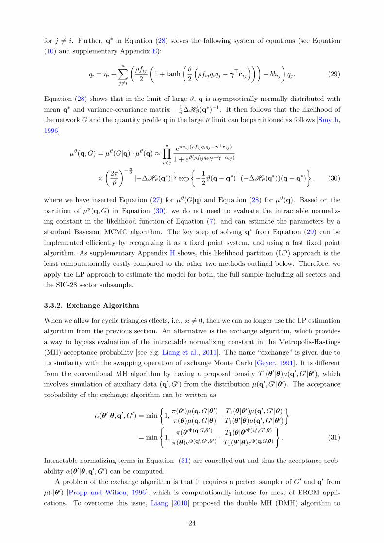
for j = i. Further, q∗ in Equation (28) solves the following system of equations (see Equation(10) and supplementary Appendix E):
qi = ηi +
n∑j =i
(ρfij2
(1 + tanh
(ϑ
2
(ρfijqiqj − γ⊤cij
)))− bbij
)qj . (29)
Equation (28) shows that in the limit of large ϑ, q is asymptotically normally distributed withmean q∗ and variance-covariance matrix − 1
ϑ∆Hϑ(q∗)−1. It then follows that the likelihood of
the network G and the quantity profile q in the large ϑ limit can be partitioned as follows [Smyth,1996]
µϑ(q, G) = µϑ(G|q) · µϑ(q) ≈n∏i<j
eϑaij(ρfijqiqj−γ⊤cij)
1 + eϑ(ρfijqiqj−γ⊤cij)
×(2π
ϑ
)−n2
|−∆Hϑ(q∗)|
12 exp
−1
2ϑ(q− q∗)⊤(−∆Hϑ(q
∗))(q− q∗)
, (30)
where we have inserted Equation (27) for µϑ(G|q) and Equation (28) for µϑ(q). Based on thepartition of µϑ(q, G) in Equation (30), we do not need to evaluate the intractable normaliz-ing constant in the likelihood function of Equation (7), and can estimate the parameters by astandard Bayesian MCMC algorithm. The key step of solving q∗ from Equation (29) can beimplemented efficiently by recognizing it as a fixed point system, and using a fast fixed pointalgorithm. As supplementary Appendix H shows, this likelihood partition (LP) approach is theleast computationally costly compared to the other two methods outlined below. Therefore, weapply the LP approach to estimate the model for both, the full sample including all sectors andthe SIC-28 sector subsample.
3.3.2. Exchange Algorithm
When we allow for cyclic triangles effects, i.e., κ = 0, then we can no longer use the LP estimationalgorithm from the previous section. An alternative is the exchange algorithm, which providesa way to bypass evaluation of the intractable normalizing constant in the Metropolis-Hastings(MH) acceptance probability [see e.g. Liang et al., 2011]. The name “exchange” is given due toits similarity with the swapping operation of exchange Monte Carlo [Geyer, 1991]. It is differentfrom the conventional MH algorithm by having a proposal density T1(θ
′|θ)µ(q′, G′|θ′), whichinvolves simulation of auxiliary data (q′, G′) from the distribution µ(q′, G′|θ′). The acceptanceprobability of the exchange algorithm can be written as
α(θ′|θ,q′, G′) = min
1,π(θ′)µ(q, G|θ′)
π(θ)µ(q, G|θ)· T1(θ|θ
′)µ(q′, G′|θ)T1(θ′|θ)µ(q′, G′|θ′)
= min
1,
π(θ′Φ(q,G,θ′)
π(θ)eΦ(q′,G′,θ′)· T1(θ|θ
′Φ(q′,G′,θ)
T1(θ′|θ)eΦ(q,G,θ)
. (31)
Intractable normalizing terms in Equation (31) are cancelled out and thus the acceptance prob-ability α(θ′|θ,q′, G′) can be computed.
A problem of the exchange algorithm is that it requires a perfect sampler of G′ and q′ fromµ(·|θ′) [Propp and Wilson, 1996], which is computationally intense for most of ERGM appli-cations. To overcome this issue, Liang [2010] proposed the double MH (DMH) algorithm to
24
replace the perfect sampler with a finite MH chain initialized at the observed network. In thispaper, we use the DMH algorithm for parameter estimation, and more specific details about itsimplementation can be found in supplementary Appendix G.1.
To improve the computational efficiency of the DMH algorithm, we assume that during thedynamic network formation process, whenever a firm changes its R&D collaborations, all firmsadjust output levels immediately and thus the new output levels will be the profit-maximizingoutput given by the best response function q∗ = M(G)−1η plus a stochastic error term.41 Thesize of error, according to the approximation derived in supplementary Appendix G.4, shouldbe determined by M(G)−1. This assumption means that we impose two different time scales: afast time scale of output adjustments, and a slow time scale of link adjustments [Khalil, 2002].42
When simulating auxiliary data for the output levels and the network, this assumption savesfirm’s infinitesimal adjustments on output and turns it into an implicit function of the network.However, we will have to evaluate M(G)−1 whenever a link has been added or removed from theauxiliary network and this may still be computationally costly. To do this in an efficient way, weuse a matrix perturbation result that is derived in supplementary Appendix G.5.
3.3.3. Adaptive Exchange Algorithm
Even though the DMH algorithm alleviates the computational burden by replacing perfect sam-pling, convergence of the finite MH chain in the DMH algorithm is not theoretically guaranteed.Therefore, the DMH estimates are only approximately correct no matter how long the algorithmhas been run. Especially, if the network distribution represented by an ERGM is multi-modal,the finite MH run may be trapped at one of the local maxima of the likelihood function (“localtrap problem”). Consequentially, the Markov chain of the DMH algorithm may mix very slowlyand require unaffordable computation time for achieving convergence [Bhamidi et al., 2011].43
In this paper, we therefore use an adaptive exchange (AEX) algorithm, which has recentlybeen developed by Jin et al. [2013] and Liang et al. [2015], to overcome the uncertainty of slowmixing faced by the DMH algorithm. The foundation of the AEX algorithm is an MCMC samplingscheme called stochastic approximation Monte Carlo (SAMC) algorithm [Liang et al., 2007]. Themain feature of SAMC is that it applies importance sampling to prevent the local trap problem.In SAMC, the sample space is partitioned into non-overlapping subregions. Different importanceweights are assigned to each subregion so that SAMC draws samples from a kind of “mixturedistribution” that avoids being trapped by a local extremum. Additionally, SAMC contains aself-adjusting mechanism to the weights of each subregion so that it can escape from local extremaof the likelihood function very quickly.
41Note that q∗ maximizes the potential function of (25) for an exogenously given network G.42Observe that the stationary distribution µ(q, G) in Equation (7) does not depend on the parameter χ that
governs the speed of the output adjustment. This means that the stationary distribution µ(q, G) is independentof how quickly the output levels adjust. As a consequence, we can use it as a degree of freedom in our estimationalgorithms, that is, the stationary distribution is not affected whether we make the time scale separation assumptionor not.
43To overcome the local trap problem and thus speed up convergence during network simulation, Snijders [2002]and Mele [2017] proposed MH samplers which consist of both local and non-local steps. In the local step, only onerandom edge is updated in an iteration. With a certain probability, the sampler will implement the non-local stepwhere multiple (or even all) edges are updated in an iteration. Although Mele [2017] used a simulation study todemonstrate convergence of the MH sampler with a non-local step, the simulation result is based on a simple modelspecification with one indirect link effect and may not be extended to a more general case. Therefore, it is stillquestionable whether the finite MH runs with non-local steps can always achieve convergence for general ERGMs.
25

In the AEX algorithm, two Markov chains are running in parallel. In the first chain, we drawauxiliary data (q, G) from a family of distributions µ(q, G|θ1), . . . , µ(q, G|θm) with frequenciesdetermined by the SAMC algorithm, where (θ1, . . . ,θm) are pre-specified parameter points. Inpractice, we set m = 50 and (θ1, . . . ,θ50) are chosen by the Max-Min procedure from the DMHdraws [Liang et al., 2015]. We have also tried m = 30 and m = 100 in the simulation andempirical studies and the results are largely similar. In the second chain, we implement theexchange algorithm for updating the target parameters, where auxiliary data, q′ and G′, arere-sampled from the first chain by an importance sampling procedure. Convergence of the AEXalgorithm, i.e. q′ and G′ from the importance sampling procedure of the AEX converge to µ(·|θ′)
and the draws of θ from the target chain will converge weakly to the posterior µ(θ|q, G), can beshown when the number of iterations of both the auxiliary and target chains go to infinity. Detailsof implementing the AEX algorithm and the proof of convergence are provided in supplementaryAppendices G.2 and G.3.
3.4. Empirical Results
Table 2 presents our estimation results for the full sample of all sectors and the subsamplerestricted to the SIC-28 sector.44 Due to the aforementioned computational constraints, we onlyapply the LP algorithm to estimate the full sample, while applying all three estimation algorithmsto the subsample of the SIC-28 sector. In the full sample, the result shows that both estimatesof the technology spillover parameter ρ (0.0355) and the competition parameter b (0.0002) aresignificant and have the expected signs. The two effects match our theoretical predictions fromSection 2, showing that firms face a positive complementary effect from R&D collaborations and anegative substitution effect from competing firms in the same market. Furthermore, we find thatthe technology spillover effect ρ is much larger than the product market rivalry effect b [Bloomet al., 2013]. This suggests that the marginal returns from R&D collaborations are positive evenbetween competing firms. We also find that a higher labor productivity is associated with higherR&D expenditures [see e.g., Cohen et al., 1987]. The estimation results further show significanteffects from the control variables in the linking cost function, including the same sector (at 3-digitSIC level) and the same country dummies, and the sum of log patent counts from each of the twofirms involved in a collaboration. Results on the two dummies reveal that the R&D collaborationcost would be lower among two firms in the same sector or in the same country. The sum ofthe log patent numbers acts as a proxy for the research capacities of collaborating firms [Hanakiet al., 2010] and a higher value indicates lower R&D collaboration cost between them.
In the SIC-28 subsample, the estimates are similar across different estimation methods, whichshows the robustness of the estimates. Compared to the result of the full sample, there areadditional significant effects from the differences in productivities between collaborating firmsand its square in the linking cost. This non-monotonic effect from the differences in productiv-ities indicates that R&D collaborations between similar but not too similar firms involve lowercollaboration and coordination costs [see e.g. Hanaki et al., 2010; Nooteboom et al., 2007].
In Table 3 we provide additional estimation results by taking into account heterogeneoustechnology spillover effects among collaborating firms. We also allow for a cyclic triangles effectsin the linking cost function, where firms with common collaborators may experience lower col-
44The estimation result of the SIC-36 sector is available in Appendix I.
26
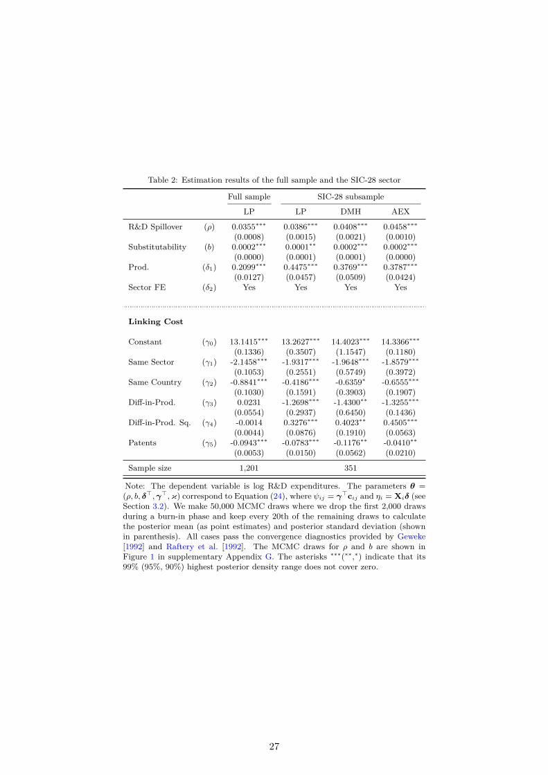
Table 2: Estimation results of the full sample and the SIC-28 sector
Full sample SIC-28 subsample
LP LP DMH AEX
R&D Spillover (ρ) 0.0355∗∗∗ 0.0386∗∗∗ 0.0408∗∗∗ 0.0458∗∗∗
(0.0008) (0.0015) (0.0021) (0.0010)Substitutability (b) 0.0002∗∗∗ 0.0001∗∗ 0.0002∗∗∗ 0.0002∗∗∗
(0.0000) (0.0001) (0.0001) (0.0000)Prod. (δ1) 0.2099∗∗∗ 0.4475∗∗∗ 0.3769∗∗∗ 0.3787∗∗∗
(0.0127) (0.0457) (0.0509) (0.0424)Sector FE (δ2) Yes Yes Yes Yes
Linking Cost
Constant (γ0) 13.1415∗∗∗ 13.2627∗∗∗ 14.4023∗∗∗ 14.3366∗∗∗
(0.1336) (0.3507) (1.1547) (0.1180)Same Sector (γ1) -2.1458∗∗∗ -1.9317∗∗∗ -1.9648∗∗∗ -1.8579∗∗∗
(0.1053) (0.2551) (0.5749) (0.3972)Same Country (γ2) -0.8841∗∗∗ -0.4186∗∗∗ -0.6359∗ -0.6555∗∗∗
(0.1030) (0.1591) (0.3903) (0.1907)Diff-in-Prod. (γ3) 0.0231 -1.2698∗∗∗ -1.4300∗∗ -1.3255∗∗∗
(0.0554) (0.2937) (0.6450) (0.1436)Diff-in-Prod. Sq. (γ4) -0.0014 0.3276∗∗∗ 0.4023∗∗ 0.4505∗∗∗
(0.0044) (0.0876) (0.1910) (0.0563)Patents (γ5) -0.0943∗∗∗ -0.0783∗∗∗ -0.1176∗∗ -0.0410∗∗
(0.0053) (0.0150) (0.0562) (0.0210)
Sample size 1,201 351
Note: The dependent variable is log R&D expenditures. The parameters θ =(ρ, b, δ⊤,γ⊤,κ) correspond to Equation (24), where ψij = γ⊤cij and ηi = Xiδ (seeSection 3.2). We make 50,000 MCMC draws where we drop the first 2,000 drawsduring a burn-in phase and keep every 20th of the remaining draws to calculatethe posterior mean (as point estimates) and posterior standard deviation (shownin parenthesis). All cases pass the convergence diagnostics provided by Geweke[1992] and Raftery et al. [1992]. The MCMC draws for ρ and b are shown inFigure 1 in supplementary Appendix G. The asterisks ∗∗∗(∗∗,∗) indicate that its99% (95%, 90%) highest posterior density range does not cover zero.
27
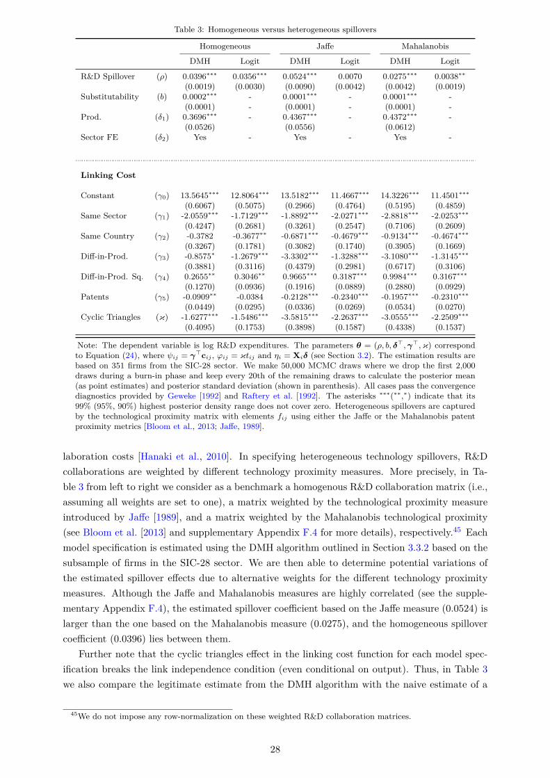
Table 3: Homogeneous versus heterogeneous spillovers
Homogeneous Jaffe Mahalanobis
DMH Logit DMH Logit DMH Logit
R&D Spillover (ρ) 0.0396∗∗∗ 0.0356∗∗∗ 0.0524∗∗∗ 0.0070 0.0275∗∗∗ 0.0038∗∗
(0.0019) (0.0030) (0.0090) (0.0042) (0.0042) (0.0019)Substitutability (b) 0.0002∗∗∗ - 0.0001∗∗∗ - 0.0001∗∗∗ -
(0.0001) - (0.0001) - (0.0001) -Prod. (δ1) 0.3696∗∗∗ - 0.4367∗∗∗ - 0.4372∗∗∗ -
(0.0526) (0.0556) (0.0612)Sector FE (δ2) Yes - Yes - Yes -
Linking Cost
Constant (γ0) 13.5645∗∗∗ 12.8064∗∗∗ 13.5182∗∗∗ 11.4667∗∗∗ 14.3226∗∗∗ 11.4501∗∗∗
(0.6067) (0.5075) (0.2966) (0.4764) (0.5195) (0.4859)Same Sector (γ1) -2.0559∗∗∗ -1.7129∗∗∗ -1.8892∗∗∗ -2.0271∗∗∗ -2.8818∗∗∗ -2.0253∗∗∗
(0.4247) (0.2681) (0.3261) (0.2547) (0.7106) (0.2609)Same Country (γ2) -0.3782 -0.3677∗∗ -0.6871∗∗∗ -0.4679∗∗∗ -0.9134∗∗∗ -0.4674∗∗∗
(0.3267) (0.1781) (0.3082) (0.1740) (0.3905) (0.1669)Diff-in-Prod. (γ3) -0.8575∗ -1.2679∗∗∗ -3.3302∗∗∗ -1.3288∗∗∗ -3.1080∗∗∗ -1.3145∗∗∗
(0.3881) (0.3116) (0.4379) (0.2981) (0.6717) (0.3106)Diff-in-Prod. Sq. (γ4) 0.2655∗∗ 0.3046∗∗ 0.9665∗∗∗ 0.3187∗∗∗ 0.9984∗∗∗ 0.3167∗∗∗
(0.1270) (0.0936) (0.1916) (0.0889) (0.2880) (0.0929)Patents (γ5) -0.0909∗∗ -0.0384 -0.2128∗∗∗ -0.2340∗∗∗ -0.1957∗∗∗ -0.2310∗∗∗
(0.0449) (0.0295) (0.0336) (0.0269) (0.0534) (0.0270)Cyclic Triangles (κ) -1.6277∗∗∗ -1.5486∗∗∗ -3.5815∗∗∗ -2.2637∗∗∗ -3.0555∗∗∗ -2.2509∗∗∗
(0.4095) (0.1753) (0.3898) (0.1587) (0.4338) (0.1537)
Note: The dependent variable is log R&D expenditures. The parameters θ = (ρ, b, δ⊤,γ⊤,κ) correspondto Equation (24), where ψij = γ⊤cij , φij = κtij and ηi = Xiδ (see Section 3.2). The estimation results arebased on 351 firms from the SIC-28 sector. We make 50,000 MCMC draws where we drop the first 2,000draws during a burn-in phase and keep every 20th of the remaining draws to calculate the posterior mean(as point estimates) and posterior standard deviation (shown in parenthesis). All cases pass the convergencediagnostics provided by Geweke [1992] and Raftery et al. [1992]. The asterisks ∗∗∗(∗∗,∗) indicate that its99% (95%, 90%) highest posterior density range does not cover zero. Heterogeneous spillovers are capturedby the technological proximity matrix with elements fij using either the Jaffe or the Mahalanobis patentproximity metrics [Bloom et al., 2013; Jaffe, 1989].
laboration costs [Hanaki et al., 2010]. In specifying heterogeneous technology spillovers, R&Dcollaborations are weighted by different technology proximity measures. More precisely, in Ta-ble 3 from left to right we consider as a benchmark a homogenous R&D collaboration matrix (i.e.,assuming all weights are set to one), a matrix weighted by the technological proximity measureintroduced by Jaffe [1989], and a matrix weighted by the Mahalanobis technological proximity(see Bloom et al. [2013] and supplementary Appendix F.4 for more details), respectively.45 Eachmodel specification is estimated using the DMH algorithm outlined in Section 3.3.2 based on thesubsample of firms in the SIC-28 sector. We are then able to determine potential variations ofthe estimated spillover effects due to alternative weights for the different technology proximitymeasures. Although the Jaffe and Mahalanobis measures are highly correlated (see the supple-mentary Appendix F.4), the estimated spillover coefficient based on the Jaffe measure (0.0524) islarger than the one based on the Mahalanobis measure (0.0275), and the homogeneous spillovercoefficient (0.0396) lies between them.
Further note that the cyclic triangles effect in the linking cost function for each model spec-ification breaks the link independence condition (even conditional on output). Thus, in Table 3we also compare the legitimate estimate from the DMH algorithm with the naive estimate of a
45We do not impose any row-normalization on these weighted R&D collaboration matrices.
28
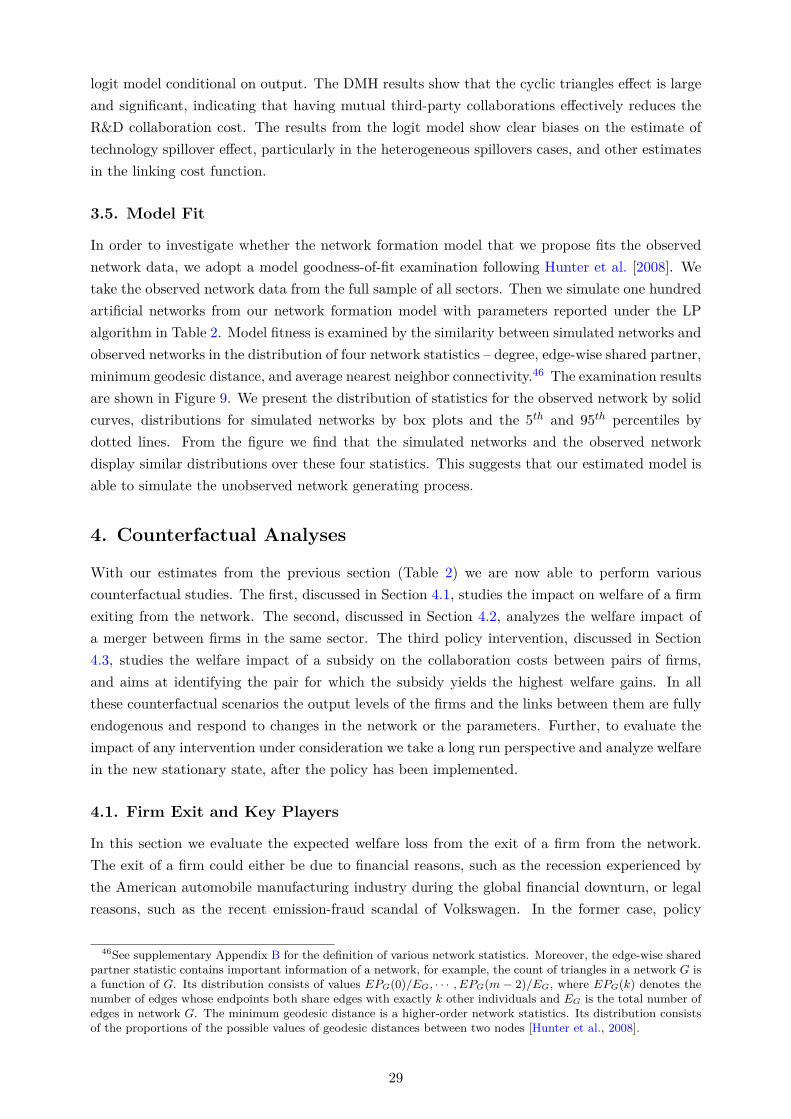
logit model conditional on output. The DMH results show that the cyclic triangles effect is largeand significant, indicating that having mutual third-party collaborations effectively reduces theR&D collaboration cost. The results from the logit model show clear biases on the estimate oftechnology spillover effect, particularly in the heterogeneous spillovers cases, and other estimatesin the linking cost function.
3.5. Model Fit
In order to investigate whether the network formation model that we propose fits the observednetwork data, we adopt a model goodness-of-fit examination following Hunter et al. [2008]. Wetake the observed network data from the full sample of all sectors. Then we simulate one hundredartificial networks from our network formation model with parameters reported under the LPalgorithm in Table 2. Model fitness is examined by the similarity between simulated networks andobserved networks in the distribution of four network statistics – degree, edge-wise shared partner,minimum geodesic distance, and average nearest neighbor connectivity.46 The examination resultsare shown in Figure 9. We present the distribution of statistics for the observed network by solidcurves, distributions for simulated networks by box plots and the 5th and 95th percentiles bydotted lines. From the figure we find that the simulated networks and the observed networkdisplay similar distributions over these four statistics. This suggests that our estimated model isable to simulate the unobserved network generating process.
4. Counterfactual Analyses
With our estimates from the previous section (Table 2) we are now able to perform variouscounterfactual studies. The first, discussed in Section 4.1, studies the impact on welfare of a firmexiting from the network. The second, discussed in Section 4.2, analyzes the welfare impact ofa merger between firms in the same sector. The third policy intervention, discussed in Section4.3, studies the welfare impact of a subsidy on the collaboration costs between pairs of firms,and aims at identifying the pair for which the subsidy yields the highest welfare gains. In allthese counterfactual scenarios the output levels of the firms and the links between them are fullyendogenous and respond to changes in the network or the parameters. Further, to evaluate theimpact of any intervention under consideration we take a long run perspective and analyze welfarein the new stationary state, after the policy has been implemented.
4.1. Firm Exit and Key Players
In this section we evaluate the expected welfare loss from the exit of a firm from the network.The exit of a firm could either be due to financial reasons, such as the recession experienced bythe American automobile manufacturing industry during the global financial downturn, or legalreasons, such as the recent emission-fraud scandal of Volkswagen. In the former case, policy
46See supplementary Appendix B for the definition of various network statistics. Moreover, the edge-wise sharedpartner statistic contains important information of a network, for example, the count of triangles in a network G isa function of G. Its distribution consists of values EPG(0)/EG, · · · , EPG(m − 2)/EG, where EPG(k) denotes thenumber of edges whose endpoints both share edges with exactly k other individuals and EG is the total number ofedges in network G. The minimum geodesic distance is a higher-order network statistics. Its distribution consistsof the proportions of the possible values of geodesic distances between two nodes [Hunter et al., 2008].
29
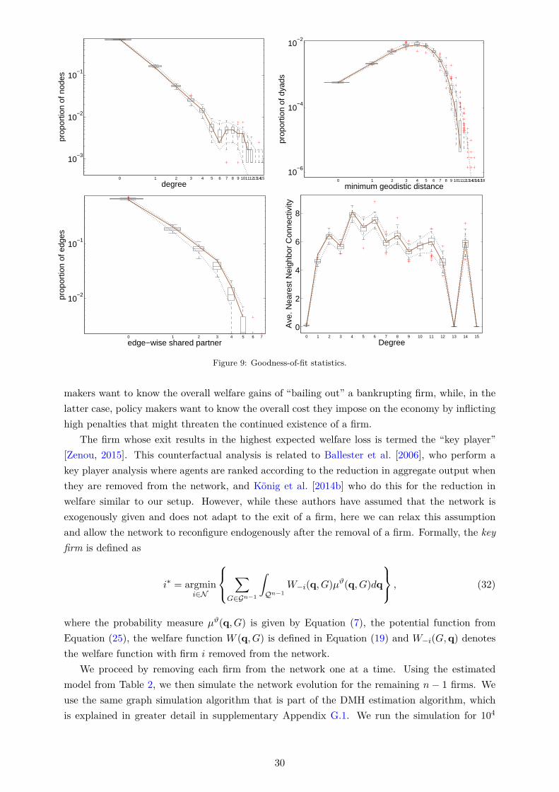
10−3
10−2
10−1
0 1 2 3 4 5 6 7 8 9 101112131415
degree
prop
ortio
n of
nod
es
10−6
10−4
10−2
0 1 2 3 4 5 6 7 8 9 101112131415161718
minimum geodistic distance
prop
ortio
n of
dya
ds
10−2
10−1
0 1 2 3 4 5 6 7
edge−wise shared partner
prop
ortio
n of
edg
es
0
2
4
6
8
0 1 2 3 4 5 6 7 8 9 10 11 12 13 14 15
Degree
Ave
. Nea
rest
Nei
ghbo
r C
onne
ctiv
ity
Figure 9: Goodness-of-fit statistics.
makers want to know the overall welfare gains of “bailing out” a bankrupting firm, while, in thelatter case, policy makers want to know the overall cost they impose on the economy by inflictinghigh penalties that might threaten the continued existence of a firm.
The firm whose exit results in the highest expected welfare loss is termed the “key player”[Zenou, 2015]. This counterfactual analysis is related to Ballester et al. [2006], who perform akey player analysis where agents are ranked according to the reduction in aggregate output whenthey are removed from the network, and König et al. [2014b] who do this for the reduction inwelfare similar to our setup. However, while these authors have assumed that the network isexogenously given and does not adapt to the exit of a firm, here we can relax this assumptionand allow the network to reconfigure endogenously after the removal of a firm. Formally, the keyfirm is defined as
i∗ = argmini∈N
∑G∈Gn−1
∫Qn−1
W−i(q, G)µϑ(q, G)dq
, (32)
where the probability measure µϑ(q, G) is given by Equation (7), the potential function fromEquation (25), the welfare function W (q, G) is defined in Equation (19) and W−i(G,q) denotesthe welfare function with firm i removed from the network.
We proceed by removing each firm from the network one at a time. Using the estimatedmodel from Table 2, we then simulate the network evolution for the remaining n − 1 firms. Weuse the same graph simulation algorithm that is part of the DMH estimation algorithm, whichis explained in greater detail in supplementary Appendix G.1. We run the simulation for 104
30
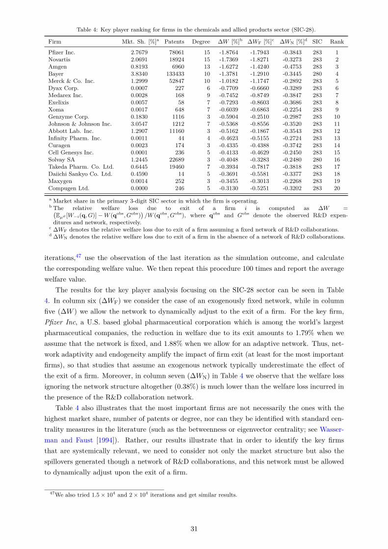
Table 4: Key player ranking for firms in the chemicals and allied products sector (SIC-28).
Firm Mkt. Sh. [%]a Patents Degree ∆W [%]b ∆WF [%]c ∆WN [%]d SIC Rank
Pfizer Inc. 2.7679 78061 15 -1.8764 -1.7943 -0.3843 283 1Novartis 2.0691 18924 15 -1.7369 -1.8271 -0.3273 283 2Amgen 0.8193 6960 13 -1.6272 -1.4240 -0.4753 283 3Bayer 3.8340 133433 10 -1.3781 -1.2910 -0.3445 280 4Merck & Co. Inc. 1.2999 52847 10 -1.0182 -1.1747 -0.2892 283 5Dyax Corp. 0.0007 227 6 -0.7709 -0.6660 -0.3289 283 6Medarex Inc. 0.0028 168 9 -0.7452 -0.8749 -0.3847 283 7Exelixis 0.0057 58 7 -0.7293 -0.8603 -0.3686 283 8Xoma 0.0017 648 7 -0.6039 -0.6863 -0.2254 283 9Genzyme Corp. 0.1830 1116 3 -0.5904 -0.2510 -0.2987 283 10Johnson & Johnson Inc. 3.0547 1212 7 -0.5368 -0.8556 -0.3520 283 11Abbott Lab. Inc. 1.2907 11160 3 -0.5162 -0.1867 -0.3543 283 12Infinity Pharm. Inc. 0.0011 44 4 -0.4623 -0.5155 -0.2724 283 13Curagen 0.0023 174 3 -0.4335 -0.4388 -0.3742 283 14Cell Genesys Inc. 0.0001 236 5 -0.4133 -0.4629 -0.2450 283 15Solvay SA 1.2445 22689 3 -0.4048 -0.3283 -0.2480 280 16Takeda Pharm. Co. Ltd. 0.6445 19460 7 -0.3934 -0.7817 -0.3818 283 17Daiichi Sankyo Co. Ltd. 0.4590 14 5 -0.3691 -0.5581 -0.3377 283 18Maxygen 0.0014 252 3 -0.3455 -0.3013 -0.2268 283 19Compugen Ltd. 0.0000 246 5 -0.3130 -0.5251 -0.3202 283 20a Market share in the primary 3-digit SIC sector in which the firm is operating.b The relative welfare loss due to exit of a firm i is computed as ∆W =(
Eµϑ [W−i(q, G)]−W (qobs, Gobs))/W (qobs, Gobs), where qobs and Gobs denote the observed R&D expen-
ditures and network, respectively.c ∆WF denotes the relative welfare loss due to exit of a firm assuming a fixed network of R&D collaborations.d ∆WN denotes the relative welfare loss due to exit of a firm in the absence of a network of R&D collaborations.
iterations,47 use the observation of the last iteration as the simulation outcome, and calculatethe corresponding welfare value. We then repeat this procedure 100 times and report the averagewelfare value.
The results for the key player analysis focusing on the SIC-28 sector can be seen in Table4. In column six (∆WF) we consider the case of an exogenously fixed network, while in columnfive (∆W ) we allow the network to dynamically adjust to the exit of a firm. For the key firm,Pfizer Inc, a U.S. based global pharmaceutical corporation which is among the world’s largestpharmaceutical companies, the reduction in welfare due to its exit amounts to 1.79% when weassume that the network is fixed, and 1.88% when we allow for an adaptive network. Thus, net-work adaptivity and endogeneity amplify the impact of firm exit (at least for the most importantfirms), so that studies that assume an exogenous network typically underestimate the effect ofthe exit of a firm. Moreover, in column seven (∆WN) in Table 4 we observe that the welfare lossignoring the network structure altogether (0.38%) is much lower than the welfare loss incurred inthe presence of the R&D collaboration network.
Table 4 also illustrates that the most important firms are not necessarily the ones with thehighest market share, number of patents or degree, nor can they be identified with standard cen-trality measures in the literature (such as the betweenness or eigenvector centrality; see Wasser-man and Faust [1994]). Rather, our results illustrate that in order to identify the key firmsthat are systemically relevant, we need to consider not only the market structure but also thespillovers generated though a network of R&D collaborations, and this network must be allowedto dynamically adjust upon the exit of a firm.
47We also tried 1.5× 10⁴ and 2× 10⁴ iterations and get similar results.
31
4.2. Mergers and Acquisitions
Our framework can also be used to study the counterfactual scenario for mergers and acquisitionsin innovative industries, and their impact on welfare [Farrell and Shapiro, 1990; Salant et al.,1983]. Market concentration indices are not adequate to correctly account for the network effectsof a merger on welfare [see e.g. Encaoua and Hollander, 2002]. This is because the effect of amerger of two firms on industry profits, consumer surplus, and overall welfare depends not only onthe market structure (as for example in Bimpikis et al. [2014]), but also on the R&D spillovers inthe network which might lead to R&D-efficiency gains from concentration. Due to these spillovers,mergers and the increased concentration they generate (both, in terms of the product market andthe collaboration network) can be good or bad for welfare [Daughety, 1990], depending on theidentities of the involved firms and their positions in the market as well as the network structure.This counterfactual analysis is therefore potentially important for antitrust policy makers. Forexample, in 2014, more than half of the merger proposals that were investigated by the U.S.Department of Justice involved R&D-efficiency claims [Marshall and Parra, 2015].
Based on our model we can assess the impact of a merger between two firms i and j which arecompeting in the same market. The merger that results (in expectation) in the greatest reductionin welfare is defined as
(i, j)∗ = argmin(i,j)∈N×N
∑G∈Gn−1
∫Qn−1
Wi∪j(q, G)µϑ(q, G)dq
, (33)
where the probability measure µϑ(q, G) is given by Equation (7), the potential function fromEquation (25), the welfare function W (q, G) is defined in Equation (19) and Wi∪j(q, G) denotesthe welfare function with firms i and j being merged to a single firm k in the network G. That is,two incident nodes, i and j in G, are merged into a new node k, where each of the edges incidentto k correspond to an edge incident to either i or j. In a similar way, the merger that results (inexpectation) in the greatest increase in welfare can be defined.48
Using the same simulation procedure as in Section 4.1, the merger rankings (for both, welfaregains and losses) can be found in Table 5. To prevent ambiguity on the sector identity of themerged firms, we restrict mergers to firms within the same 3-digit SIC sectors. The ranking fora fixed network in column ten (∆WF) in Table 5 is based on the assumption that the networkdoes not adjust to the merger and can be interpreted as a short run analysis. In contrast, theranking in column nine (∆W ) is based on an endogenous network which adapts to a merger andcan be interpreted as a long run analysis. The mergers resulting in the highest reduction or gainin welfare involve only firms in the drugs development sector (SIC 283), which is also the largestsector in our sample.
The highest loss in the endogenous network case is triggered by a merger between DaiichiSankyo Co. Ltd., a global pharmaceutical company and the second largest pharmaceutical com-pany in Japan, and Schering-Plough Corp., a U.S.-based pharmaceutical company, yielding areduction in welfare of 0.6%. The relatively large market shares of these companies amplify the
48We note that we only consider mergers between firms in the same market. We also do not consider firmsoperating in multiple markets simultaneously, such as for example in Bimpikis et al. [2014]. However, we believethat our analysis of a very specific type of a merger can generate useful insights because it takes into accountmultiple sources of externalities that are typically ignored in other studies.
32
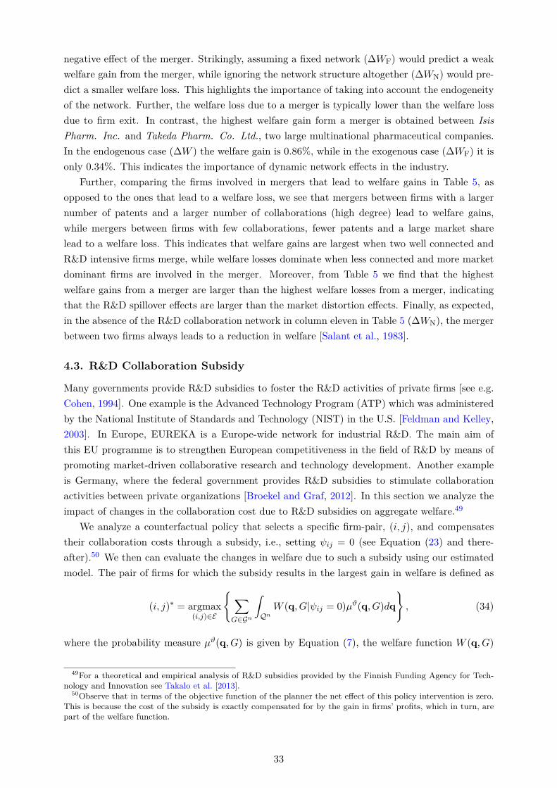
negative effect of the merger. Strikingly, assuming a fixed network (∆WF) would predict a weakwelfare gain from the merger, while ignoring the network structure altogether (∆WN) would pre-dict a smaller welfare loss. This highlights the importance of taking into account the endogeneityof the network. Further, the welfare loss due to a merger is typically lower than the welfare lossdue to firm exit. In contrast, the highest welfare gain form a merger is obtained between IsisPharm. Inc. and Takeda Pharm. Co. Ltd., two large multinational pharmaceutical companies.In the endogenous case (∆W ) the welfare gain is 0.86%, while in the exogenous case (∆WF) it isonly 0.34%. This indicates the importance of dynamic network effects in the industry.
Further, comparing the firms involved in mergers that lead to welfare gains in Table 5, asopposed to the ones that lead to a welfare loss, we see that mergers between firms with a largernumber of patents and a larger number of collaborations (high degree) lead to welfare gains,while mergers between firms with few collaborations, fewer patents and a large market sharelead to a welfare loss. This indicates that welfare gains are largest when two well connected andR&D intensive firms merge, while welfare losses dominate when less connected and more marketdominant firms are involved in the merger. Moreover, from Table 5 we find that the highestwelfare gains from a merger are larger than the highest welfare losses from a merger, indicatingthat the R&D spillover effects are larger than the market distortion effects. Finally, as expected,in the absence of the R&D collaboration network in column eleven in Table 5 (∆WN), the mergerbetween two firms always leads to a reduction in welfare [Salant et al., 1983].
4.3. R&D Collaboration Subsidy
Many governments provide R&D subsidies to foster the R&D activities of private firms [see e.g.Cohen, 1994]. One example is the Advanced Technology Program (ATP) which was administeredby the National Institute of Standards and Technology (NIST) in the U.S. [Feldman and Kelley,2003]. In Europe, EUREKA is a Europe-wide network for industrial R&D. The main aim ofthis EU programme is to strengthen European competitiveness in the field of R&D by means ofpromoting market-driven collaborative research and technology development. Another exampleis Germany, where the federal government provides R&D subsidies to stimulate collaborationactivities between private organizations [Broekel and Graf, 2012]. In this section we analyze theimpact of changes in the collaboration cost due to R&D subsidies on aggregate welfare.49
We analyze a counterfactual policy that selects a specific firm-pair, (i, j), and compensatestheir collaboration costs through a subsidy, i.e., setting ψij = 0 (see Equation (23) and there-after).50 We then can evaluate the changes in welfare due to such a subsidy using our estimatedmodel. The pair of firms for which the subsidy results in the largest gain in welfare is defined as
(i, j)∗ = argmax(i,j)∈E
∑G∈Gn
∫Qn
W (q, G|ψij = 0)µϑ(q, G)dq
, (34)
where the probability measure µϑ(q, G) is given by Equation (7), the welfare function W (q, G)
49For a theoretical and empirical analysis of R&D subsidies provided by the Finnish Funding Agency for Tech-nology and Innovation see Takalo et al. [2013].
50Observe that in terms of the objective function of the planner the net effect of this policy intervention is zero.This is because the cost of the subsidy is exactly compensated for by the gain in firms’ profits, which in turn, arepart of the welfare function.
33
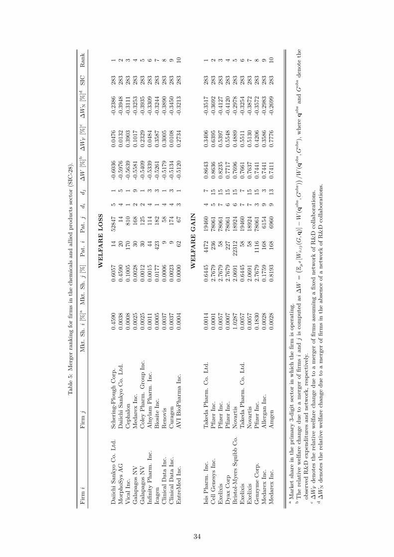
Tabl
e5:
Mer
ger
rank
ing
for
firm
sin
the
chem
ical
san
dal
lied
prod
ucts
sect
or(S
IC-2
8).
Firm
iFi
rmj
Mkt
.Sh
.i[%
]aM
kt.
Sh.j[%
]Pa
t.i
Pat.j
di
dj
∆W
[%]b
∆W
F[%
]c∆W
N[%
]dSI
CR
ank
WE
LFA
RE
LOSS
Dai
ichi
Sank
yoC
o.Lt
d.Sc
herin
g-Pl
ough
Cor
p.0.
4590
0.60
5714
5284
75
1-0
.603
60.
0476
-0.2
386
283
1M
orph
oSys
AG
Dai
ichi
Sank
yoC
o.Lt
d.0.
0038
0.45
9020
144
5-0
.597
60.
0132
-0.3
948
283
2V
ical
Inc.
Cep
halo
n0.
0008
0.10
0517
081
01
1-0
.563
90.
3903
-0.3
111
283
3G
alap
agos
NV
Med
arex
Inc.
0.00
250.
0028
3016
82
9-0
.558
10.
1017
-0.3
253
283
4G
alap
agos
NV
Col
eyPh
arm
.G
roup
Inc.
0.00
250.
0012
3012
52
1-0
.540
90.
2329
-0.3
935
283
5In
finity
Phar
m.
Inc.
Aln
ylam
Phar
m.
Inc.
0.00
110.
0015
4411
44
3-0
.533
90.
0484
-0.3
309
283
6Ic
agen
Bio
site
Inc.
0.00
050.
0177
423
182
13
-0.5
261
0.35
87-0
.324
428
37
Clin
ical
Dat
aIn
c.R
enov
is0.
0037
0.00
069
584
1-0
.517
90.
3005
-0.3
890
283
8C
linic
alD
ata
Inc.
Cur
agen
0.00
370.
0023
917
44
3-0
.513
40.
0108
-0.3
450
283
9En
treM
edIn
c.AV
IB
ioPh
arm
aIn
c.0.
0004
0.00
0062
673
1-0
.512
00.
2734
-0.3
213
283
10
WE
LFA
RE
GA
IN
Isis
Phar
m.
Inc.
Take
daPh
arm
.C
o.Lt
d.0.
0014
0.64
4544
7219
460
47
0.86
430.
3406
-0.3
517
283
1C
ellG
enes
ysIn
c.Pfi
zer
Inc.
0.00
012.
7679
236
7806
15
150.
8636
0.63
95-0
.369
228
32
Exel
ixis
Pfize
rIn
c.0.
0057
2.76
7958
7806
17
150.
8235
0.53
97-0
.412
728
33
Dya
xC
orp
Pfize
rIn
c.0.
0007
2.76
7922
778
061
615
0.77
170.
5548
-0.4
120
283
4B
risto
l-Mye
rsSq
uibb
Co.
Nov
artis
1.02
872.
0691
2231
218
924
615
0.76
960.
4889
-0.2
978
283
5Ex
elix
isTa
keda
Phar
m.
Co.
Ltd.
0.00
570.
6445
5819
460
77
0.76
610.
5511
-0.3
254
283
6Ex
elix
isN
ovar
tis0.
0057
2.06
9158
1892
47
150.
7637
0.51
30-0
.387
228
37
Gen
zym
eC
orp.
Pfize
rIn
c.0.
1830
2.76
7911
1678
061
315
0.74
410.
4206
-0.3
572
283
8M
edar
exIn
c.A
llerg
anIn
c.0.
0028
0.17
5916
861
549
30.
7441
0.35
86-0
.298
328
39
Med
arex
Inc.
Am
gen
0.00
280.
8193
168
6960
913
0.74
110.
7776
-0.2
699
283
10
aM
arke
tsh
are
inth
epr
imar
y3-d
igit
sect
orin
whi
chth
efir
mis
oper
atin
g.b
The
rela
tive
wel
fare
chan
gedu
eto
am
erge
rof
firm
si
andj
isco
mpu
ted
as∆W
=( E µ
ϑ[W
i∪j(G,q
)]−W
(qobs,G
obs)) /W
(qobs,G
obs),
whe
reqobs
andG
obs
deno
teth
eob
serv
edR
&D
expe
nditu
res
and
netw
ork,
resp
ectiv
ely.
c∆W
Fde
note
sth
ere
lativ
ew
elfa
rech
ange
due
toa
mer
ger
offir
ms
assu
min
ga
fixed
netw
ork
ofR
&D
colla
bora
tions
.d∆W
Nde
note
sth
ere
lativ
ew
elfa
rech
ange
due
toa
mer
ger
offir
ms
inth
eab
senc
eof
ane
twor
kof
R&
Dco
llabo
ratio
ns.
34
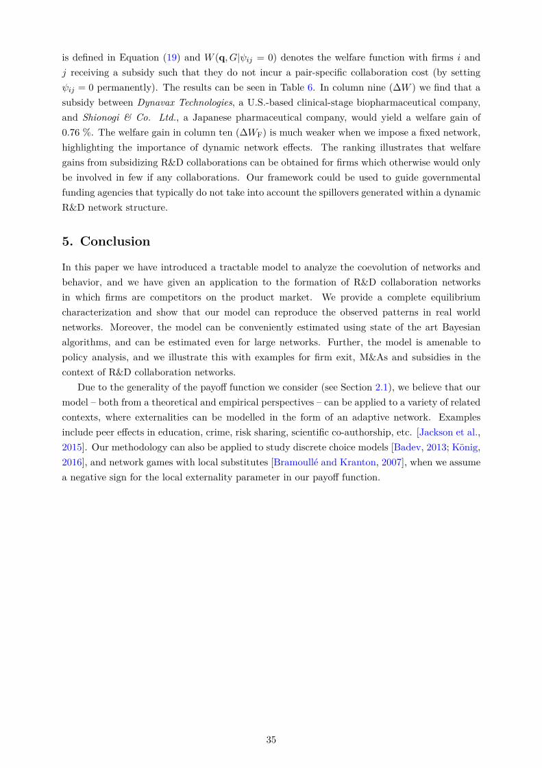
is defined in Equation (19) and W (q, G|ψij = 0) denotes the welfare function with firms i andj receiving a subsidy such that they do not incur a pair-specific collaboration cost (by settingψij = 0 permanently). The results can be seen in Table 6. In column nine (∆W ) we find that asubsidy between Dynavax Technologies, a U.S.-based clinical-stage biopharmaceutical company,and Shionogi & Co. Ltd., a Japanese pharmaceutical company, would yield a welfare gain of0.76 %. The welfare gain in column ten (∆WF) is much weaker when we impose a fixed network,highlighting the importance of dynamic network effects. The ranking illustrates that welfaregains from subsidizing R&D collaborations can be obtained for firms which otherwise would onlybe involved in few if any collaborations. Our framework could be used to guide governmentalfunding agencies that typically do not take into account the spillovers generated within a dynamicR&D network structure.
5. Conclusion
In this paper we have introduced a tractable model to analyze the coevolution of networks andbehavior, and we have given an application to the formation of R&D collaboration networksin which firms are competitors on the product market. We provide a complete equilibriumcharacterization and show that our model can reproduce the observed patterns in real worldnetworks. Moreover, the model can be conveniently estimated using state of the art Bayesianalgorithms, and can be estimated even for large networks. Further, the model is amenable topolicy analysis, and we illustrate this with examples for firm exit, M&As and subsidies in thecontext of R&D collaboration networks.
Due to the generality of the payoff function we consider (see Section 2.1), we believe that ourmodel – both from a theoretical and empirical perspectives – can be applied to a variety of relatedcontexts, where externalities can be modelled in the form of an adaptive network. Examplesinclude peer effects in education, crime, risk sharing, scientific co-authorship, etc. [Jackson et al.,2015]. Our methodology can also be applied to study discrete choice models [Badev, 2013; König,2016], and network games with local substitutes [Bramoullé and Kranton, 2007], when we assumea negative sign for the local externality parameter in our payoff function.
35
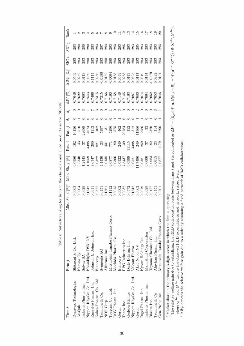
Tabl
e6:
Subs
idy
rank
ing
for
firm
sin
the
chem
ical
san
dal
lied
prod
ucts
sect
or(S
IC-2
8).
Firm
iFi
rmj
Mkt
.Sh
.i[%
]aM
kt.
Sh.j[%
]Pa
t.i
Pat.j
di
dj
∆W
[%]b
∆W
F[%
]cSI
Ci
SICj
Ran
k
Dyn
avax
Tech
nolo
gies
Shio
nogi
&C
o.Lt
d.0.
0003
0.09
8616
210
156
00
0.76
460.
0509
283
283
1A
r-Q
ule
Kem
iraO
y.0.
0004
0.33
4043
510
10
0.76
220.
0252
283
280
2In
devu
sPh
arm
.In
c.So
lvay
SA0.
0029
1.24
4537
2268
90
30.
7603
0.07
1328
328
03
Nip
pon
Kay
aku
Co.
Ltd.
Kon
inkl
ijke
DSM
NV
0.13
421.
1059
4398
4674
01
0.75
430.
0369
280
280
4En
cysiv
ePh
arm
.In
c.Jo
hnso
n&
John
son
Inc.
0.00
113.
0547
280
1212
07
0.74
660.
1111
283
283
5K
aken
Phar
m.
Co.
Ltd.
Elan
corp
0.03
770.
0322
821
462
03
0.73
150.
0986
283
283
6Ts
umur
a&
Co.
Syng
enta
AG
0.04
514.
1430
2353
970
00.
7215
-0.0
188
283
287
7N
OF
Cor
p.A
lker
mes
Inc.
0.13
610.
0138
431
310
00.
7166
0.01
3228
028
38
Toag
osei
Co.
Ltd.
Mits
ubish
iTan
abe
Phar
ma
Cor
p.0.
1412
0.08
7777
152
960
10.
7160
-0.0
004
280
283
9D
OV
Phar
m.
Inc.
Moc
hida
Phar
m.
Co.
0.00
150.
0366
8057
51
00.
7158
0.01
8828
328
310
Ger
onEl
anco
rp0.
0002
0.03
2224
046
21
30.
7146
0.00
3928
328
311
Tano
xIn
c.PP
GIn
dust
ries
Inc.
0.00
327.
5437
139
2978
40
00.
7145
0.02
8328
328
512
Ged
eon
Ric
hter
Dad
eB
ehrin
gIn
c.0.
0572
0.09
9911
115
152
00
0.71
030.
0173
283
283
13N
ippo
nK
ayak
uC
o.Lt
d.Va
lean
tPh
arm
.0.
1342
0.05
2143
9831
20
00.
7087
0.06
9528
028
314
Ger
onA
kzo
Nob
elN
V0.
0002
11.7
496
240
1136
61
20.
7080
0.01
1428
328
515
Rig
elPh
arm
.In
c.K
yorin
Hol
ding
sIn
c.0.
0019
0.03
8125
929
861
00.
7074
0.03
1928
328
316
Inde
vus
Phar
m.
Inc.
Man
nKin
dC
orpo
ratio
n0.
0029
0.00
0037
320
00.
7064
0.01
4428
328
317
Bio
site
Inc.
Toya
ma
Che
mic
alC
o.Lt
d.0.
0177
0.00
8318
223
201
00.
7062
-0.0
179
283
283
18Ts
umur
a&
Co
Aln
ylam
Phar
m.
Inc.
0.04
510.
0015
2311
40
30.
7053
0.02
2228
328
319
Gen
-Pro
beIn
c.M
itsub
ishiT
anab
ePh
arm
aC
orp.
0.02
010.
0877
1179
5296
11
0.70
460.
0101
283
283
20a
Mar
ket
shar
ein
the
prim
ary3-d
igit
sect
orin
whi
chth
efir
mis
oper
atin
g.b
The
rela
tive
wel
fare
gain
due
tosu
bsid
izin
gth
eR
&D
colla
bora
tion
cost
sbet
wee
nfir
msi
andj
isco
mpu
ted
as∆W
=( E µ
ϑ[W
(q,G
|ψij
=0)]−W
(qobs,G
obs)) /W
(qobs,G
obs),
whe
reqobs
andG
obs
deno
teth
eob
serv
edR
&D
expe
nditu
res
and
netw
ork,
resp
ectiv
ely.
c∆W
Fde
note
sth
ere
lativ
ew
elfa
rega
indu
eto
asu
bsid
yas
sum
ing
afix
edne
twor
kof
R&
Dco
llabo
ratio
ns.
36
ReferencesAiroldi, E., Goldenberg, A., Zheng, A., and Fienberg, S. (2009). A survey of statistical network models. Machine
Learning, 2(2):129–233.Anderson, S., Goeree, J., and Holt, C. (2004). Noisy directional learning and the logit equilibrium. Scandinavian
Journal of Economics, 106(3):581–602.Anderson, S. P., De Palma, A., and Thisse, J. F. (1992). Discrete choice theory of product differentiation. MIT
Press.Anderson, S. P., Goeree, J. K., and Holt, C. A. (2001). Minimum-effort coordination games: Stochastic potential
and logit equilibrium. Games and Economic Behavior, 34(2):177–199.Badev, A. (2013). Discrete games in endogenous networks: Theory and policy. University of Pennsylvania Working
Paper PSC 13–05.Ballester, C., Calvó-Armengol, A., and Zenou, Y. (2006). Who’s who in networks. wanted: The key player.
Econometrica, 74(5):1403–1417.Belhaj, M., Bervoets, S., and Deroian, F. (2016). Optimal networks in games with local complementarities.
Theoretical Economics, 11.Ben-Akiva, M. and Watanatada, T. (1981). Application of a continuous spatial choice logit model. Structural
analysis of discrete data with econometric applications, pages 320–343.Bhamidi, S., Bresler, G., Sly, A., et al. (2011). Mixing time of exponential random graphs. The Annals of Applied
Probability, 21(6):2146–2170.Bimpikis, K., Ehsani, S., and Ilkilic, R. (2014). Cournot competition in networked markets. Mimeo, Stanford
University.Bisin, A., Horst, U., and Özgür, O. (2006). Rational expectations equilibria of economies with local interactions.
Journal of Economic Theory, 127(1):74–116.Bloom, N., Schankerman, M., and Van Reenen, J. (2013). Identifying technology spillovers and product market
rivalry. Econometrica, 81(4):1347–1393.Blume, L. (1993). The statistical mechanics of strategic interaction. Games and Economic Behavior, 5(3):387–424.Blume, L. (2003). How noise matters. Games and Economic Behavior, 44(2):251–271.Boguná, M. and Pastor-Satorras, R. (2003). Class of correlated random networks with hidden variables. Physical
Review E, 68(3):036112.Bramoullé, Y. and Kranton, R. (2007). Public goods in networks. Journal of Economic Theory, 135(1):478–494.Brock, W. and Durlauf, S. (2001). Discrete choice with social interactions. Review of Economic Studies, 68(2):235–
260.Broekel, T. and Graf, H. (2012). Public research intensity and the structure of german R&D networks: a comparison
of 10 technologies. Economics of Innovation and New Technology, 21(4):345–372.Cabrales, A., Calvó-Armengol, A., and Zenou, Y. (2011). Social interactions and spillovers. Games and Economic
Behavior, 72(2):339–360.Calvo, G. A. (1983). Staggered prices in a utility-maximizing framework. Journal of Monetary Economics,
12(3):383–398.Chandrasekhar, A. and Jackson, M. (2012). Tractable and consistent random graph models. Available at SSRN
2150428.Cohen, L. (1994). When can government subsidize research joint ventures? politics, economics, and limits to
technology policy. The American Economic Review, 84(2):159–163.Cohen, W., Levin, R., and Mowery, D. (1987). Firm size and R&D intensity: a re-examination. The Journal of
Industrial Economics, 35(4):543–565.Copeland, A. and Fixler, D. (2012). Measuring the price of research and development output. Review of Income
and Wealth, 58(1):166–182.Cournot, A. (1838). Researches into the Mathematical Principles of the Theory of Wealth. Trans. N.T. Bacon, New
York: Macmillan.Czarnitzki, D., Hussinger, K., and Schneider, C. (2015). R&D collaboration with uncertain intellectual property
rights. Review of Industrial Organization, 46(2):183–204.D’Aspremont, C. and Jacquemin, A. (1988). Cooperative and noncooperative R&D in duopoly with spillovers. The
American Economic Review, 78(5):1133–1137.Daughety, A. F. (1990). Beneficial concentration. The American Economic Review, 80(5):1231–1237.Daughety, A. F. (2005). Cournot oligopoly: characterization and applications. Cambridge University Press.David, P. A. (1992). Heroes, herds and hysteresis in technological history: Thomas Edison and “The battle of the
systems” reconsidered. Industrial and Corporate Change, 1(1):129–180.Dawid, H. and Hellmann, T. (2014). The evolution of R&D networks. Journal of Economic Behavior & Organi-
zation, 105:158–172.Deijfen, M. and Kets, W. (2009). Random intersection graphs with tunable degree distribution and clustering.
Probability in the Engineering and Informational Sciences, 23(04):661–674.Ehrhardt, G., Marsili, M., and Vega-Redondo, F. (2008). Networks emerging in a volatile world. Economics
Working Papers.Encaoua, D. and Hollander, A. (2002). Competition policy and innovation. Oxford Review of Economic Policy,
18(1):63–79.Farrell, J. and Shapiro, C. (1990). Horizontal mergers: an equilibrium analysis. The American Economic Review,
80(1):107–126.Feldman, M. P. and Kelley, M. R. (2003). Leveraging research and development: Assessing the impact of the U.S.
advanced technology program. Small Business Economics, 20(2):153–165.Feri, F. (2007). Stochastic stability in networks with decay. Journal of Economic Theory, 135(1):442–457.Fosco, C., Vega-Redondo, F., and Marsili, M. (2010). Peer effects and peer avoidance: The diffusion of behavior in
coevolving networks. Journal of the European Economic Association, 8(1):169–202.Frank, O. and Strauss, D. (1986). Markov graphs. Journal of the American Statistical Association, 81(395):832–842.Gabaix, X. (2014). A sparsity-based model of bounded rationality. The Quarterly Journal of Economics, 1661:1710.
37
Gabaix, X. (2016). Power laws in economics: An introduction. The Journal of Economic Perspectives, 30(1):185–205.
Geweke, J. (1992). Evaluating the accuracy of sampling-based approaches to the calculation of posterior moments.Bayesian Statistics, pages 169–193.
Geyer, C. J. (1991). Markov chain Monte Carlo maximum likelihood. Interface Foundation of North America.Gibson, M. A. and Bruck, J. (2000). Efficient exact stochastic simulation of chemical systems with many species
and many channels. The Journal of Physical Chemistry A, 104(9):1876–1889.Goyal, S. and Moraga-Gonzalez, J. L. (2001). R&D networks. RAND Journal of Economics, 32(4):686–707.Griffith, R., Redding, S., and Van Reenen, J. (2003). R&D and absorptive capacity: Theory and empirical evidence.
Scandinavian Journal of Economics, 105(1):99–118.Grimmett, G. (2010). Probability on graphs. Cambridge University Press.Hagedoorn, J. (2002). Inter-firm R&D partnerships: an overview of major trends and patterns since 1960. Research
Policy, 31(4):477–492.Hanaki, N., Nakajima, R., and Ogura, Y. (2010). The dynamics of R&D network in the IT industry. Research
Policy, 39(3):386–399.Hiller, T. (2013). Peer effects in endogenous networks. Available at SSRN 2331810.Hojman, D. and Szeidl, A. (2008). Core and periphery in networks. Journal of Economic Theory, 139(1):295–309.Hojman, D. A. and Szeidl, A. (2006). Endogenous networks, social games, and evolution. Games and Economic
Behavior, 55(1):112–130.Horn, R. A. and Johnson, C. R. (1990). Matrix Analysis. Cambridge University Press.Hsieh, C.-s. and Lee, L.-f. (2013). Specification and estimation of network formation and network interaction
models with the exponential probability distribution. CUHK Working Paper.Hunter, D. R., Goodreau, S. M., and Handcock, M. S. (2008). Goodness of fit of social network models. Journal
of the American Statistical Association, 103(481).Jackson, M. (2008). Social and Economic Networks. Princeton University Press.Jackson, M. O., Rogers, B., and Zenou, Y. (2017). The economic consequences of social network structure. Journal
of Economic Literature, 55(1):49–95.Jackson, M. O. and Rogers, B. W. (2007). Meeting strangers and friends of friends: How random are social
networks? American Economic Review, 97(3):890–915.Jackson, M. O. and Watts, A. (2002). The evolution of social and economic networks. Journal of Economic Theory,
106(2):265–295.Jackson, M. O., Zenou, Y., et al. (2015). Games on networks. Handbook of Game Theory with Economic Applica-
tions, 4:95–163.Jaffe, A. and Trajtenberg, M. (2002). Patents, Citations, and Innovations: A Window on the Knowledge Economy.
MIT Press.Jaffe, A. B. (1989). Characterizing the technological position of firms, with application to quantifying technological
opportunity and research spillovers. Research Policy, 18(2):87 – 97.Jin, I. H., Yuan, Y., and Liang, F. (2013). Bayesian analysis for exponential random graph models using the
adaptive exchange sampler. Statistics and its interface, 6(4):559.Kandori, M., Mailath, G., and Rob, R. (1993). Learning, mutation, and long run equilibria in games. Econometrica,
61(1):29–56.Kelly, M. J., Schaan, J.-L., and Joncas, H. (2002). Managing alliance relationships: key challenges in the early
stages of collaboration. R&D Management, 32(1):11–22.Khalil, H. K. (2002). Nonlinear Systems. Prentice Hall.Kitsak, M., Riccaboni, M., Havlin, S., Pammolli, F., and Stanley, H. (2010). Scale-free models for the structure of
business firm networks. Physical Review E, 81:036117.König, M., Tessone, C., and Zenou, Y. (2014a). Nestedness in networks: A theoretical model and some applications.
Theoretical Economics, 9:695–752.König, M. D. (2016). Diffusion of behavior in dynamic networks. University of Zurich, Department of Economics
Working Paper No. 222.König, M. D., Liu, X., and Zenou, Y. (2014b). R&D networks: Theory, empirics and policy implications. CEPR
Discussion Paper No. 9872.König, M. D., Lorenz, J., and Zilibotti, F. (2016). Innovation vs. imitation and the evolution of productivity
distributions. Theoretical Economics, 11:1053–1102.Lehmann, E. L. and Casella, G. (2006). Theory of point estimation. Springer Science & Business Media.Liang, F. (2010). A double Metropolis–Hastings sampler for spatial models with intractable normalizing constants.
Journal of Statistical Computation and Simulation, 80(9):1007–1022.Liang, F., Jin, I. H., Song, Q., and Liu, J. S. (2015). An adaptive exchange algorithm for sampling from distributions
with intractable normalizing constants. Journal of the American Statistical Association, 111(513):377–393.Liang, F., Liu, C., and Carroll, R. (2011). Advanced Markov chain Monte Carlo methods: learning from past
samples, volume 714. John Wiley & Sons.Liang, F., Liu, C., and Carroll, R. J. (2007). Stochastic approximation in Monte Carlo computation. Journal of
the American Statistical Association, 102(477):305–320.Lychagin, S., Pinkse, J., Slade, M. E., and Van Reenen, J. (2016). Spillovers in space: does geography matter?
The Journal of Industrial Economics, 64(2):295–335.Mahadev, N. and Peled, U. (1995). Threshold Graphs and Related Topics. North Holland.Marshall, G. and Parra, A. (2015). Mergers in innovative industries. Mimeo, University of Illinois at Urbana-
Champaign.Marsili, M., Vega-Redondo, F., and Slanina, F. (2004). The rise and fall of a networked society: a formal model.
Proceedings of the National Academy of Sciences, 101(6):1439–1442.McFadden, D. (1976). The mathematical theory of demand models. Behavioral Travel Demand Models, pages
305–314.Mele, A. (2017). A structural model of dense network formation. Econometrica, 85(3):825–850.Monderer, D. and Shapley, L. (1996). Potential Games. Games and Economic Behavior, 14(1):124–143.
38

Nooteboom, B., Van Haverbeke, W., Duysters, G., Gilsing, V., and Van Den Oord, A. (2007). Optimal cognitivedistance and absorptive capacity. Research Policy, 36(7):1016–1034.
Norris, J. R. (1998). Markov chains. Cambridge University Press.Park, J. and Newman, M. (2004). Statistical mechanics of networks. Physical Review E, 70(6):66117.Powell, W. W., White, D. R., Koput, K. W., and Owen-Smith, J. (2005). Network dynamics and field evolution:
The growth of interorganizational collaboration in the life sciences. American Journal of Sociology, 110(4):1132–1205.
Propp, J. G. and Wilson, D. B. (1996). Exact sampling with coupled markov chains and applications to statisticalmechanics. Random Structures & Algorithms, 9(1-2):223–252.
Raftery, A. E., Lewis, S., Banfield, J. D., and Rafterv, A. E. (1992). How many iterations in the Gibbs sampler.Bayesian Statistics, page 4.
Rosenkopf, L. and Padula, G. (2008). Investigating the Microstructure of Network Evolution: Alliance Formationin the Mobile Communications Industry. Organization Science, 19(5):669–687.
Rosenkopf, L. and Schilling, M. (2007). Comparing alliance network structure across industries: Observations andexplanations. Strategic Entrepreneurship Journal, 1:191–209.
Rudin, W. (1987). Real and complex analysis. Tata McGraw-Hill Education.Salant, S. W., Switzer, S., and Reynolds, R. J. (1983). Losses from horizontal merger: the effects of an exogenous
change in industry structure on Cournot-Nash equilibrium. The Quarterly Journal of Economics, 98(2):185–199.Sandholm, W. (2010). Population games and evolutionary dynamics. MIT Press.Schilling, M. (2009). Understanding the alliance data. Strategic Management Journal, 30(3):233–260.Shalizi, C. R. and Rinaldo, A. (2013). Consistency under sampling of exponential random graph models. The
Annals of Statistics, 41(2):508–535.Smyth, G. K. (1996). Partitioned algorithms for maximum likelihood and other non-linear estimation. Statistics
and Computing, 6(3):201–216.Snijders, T. (2002). Markov chain Monte Carlo estimation of exponential random graph models. Journal of Social
Structure, 3(2):1–40.Snijders, T. A. (2001). The Statistical Evaluation of Social Network Dynamics. Sociological Methodology, 31(1):361–
395.Takalo, T., Tanayama, T., and Toivanen, O. (2013). Estimating the benefits of targeted R&D subsidies. Review
of Economics and Statistics, 95(1):255–272.Tomasello, M. V., Napoletano, M., Garas, A., and Schweitzer, F. (2016). The rise and fall of R&D networks.
Available at SSRN 2749230.Trajtenberg, M., Shiff, G., and Melamed, R. (2009). The “names game”: Harnessing inventors, patent data for
economic research. Annals of Economics and Statistics, (93/94):79–108.Wainwright, M. J. and Jordan, M. I. (2008). Graphical models, exponential families, and variational inference.
Foundations and Trends in Machine Learning, 1(1-2):1–305.Wasserman, S. and Faust, K. (1994). Social Network Analysis: Methods and Applications. Cambridge University
Press.Watts, A. (2001). A dynamic model of network formation. Games and Economic Behavior, 34(2):331–341.Westbrock, B. (2010). Natural concentration in industrial research collaboration. The RAND Journal of Economics,
41(2):351–371.Wong, R. (2001). Asymptotic approximations of integrals, volume 34. Society for Industrial Mathematics.Zenou, Y. (2015). Key players. Oxford Handbook on the Economics of Networks, Y. Bramoulle, B. Rogers and A.
Galeotti (Eds.), Oxford University Press.
39
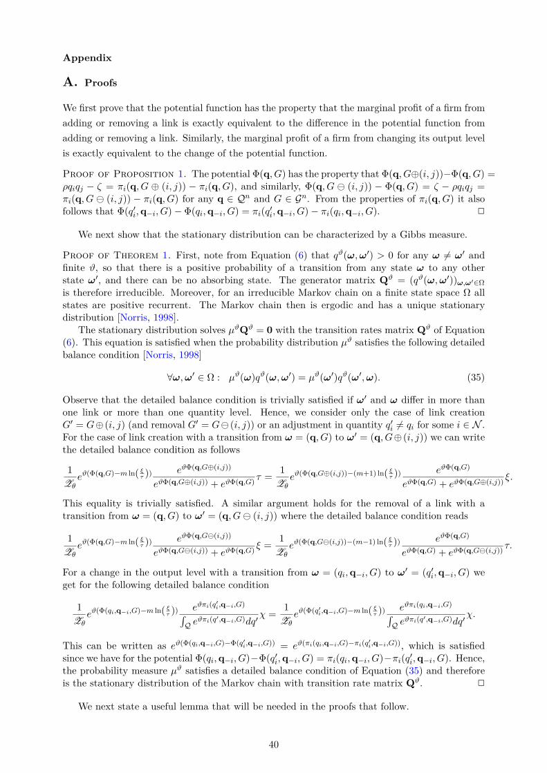
Appendix
A. Proofs
We first prove that the potential function has the property that the marginal profit of a firm fromadding or removing a link is exactly equivalent to the difference in the potential function fromadding or removing a link. Similarly, the marginal profit of a firm from changing its output levelis exactly equivalent to the change of the potential function.
Proof of Proposition 1. The potential Φ(q, G) has the property that Φ(q, G⊕(i, j))−Φ(q, G) =ρqiqj − ζ = πi(q, G ⊕ (i, j)) − πi(q, G), and similarly, Φ(q, G ⊖ (i, j)) − Φ(q, G) = ζ − ρqiqj =πi(q, G ⊖ (i, j)) − πi(q, G) for any q ∈ Qn and G ∈ Gn. From the properties of πi(q, G) it alsofollows that Φ(q′i,q−i, G)− Φ(qi,q−i, G) = πi(q
′i,q−i, G)− πi(qi,q−i, G). 2
We next show that the stationary distribution can be characterized by a Gibbs measure.
Proof of Theorem 1. First, note from Equation (6) that qϑ(ω,ω′) > 0 for any ω = ω′ andfinite ϑ, so that there is a positive probability of a transition from any state ω to any otherstate ω′, and there can be no absorbing state. The generator matrix Qϑ = (qϑ(ω,ω′))ω,ω′∈Ωis therefore irreducible. Moreover, for an irreducible Markov chain on a finite state space Ω allstates are positive recurrent. The Markov chain then is ergodic and has a unique stationarydistribution [Norris, 1998].
The stationary distribution solves µϑQϑ = 0 with the transition rates matrix Qϑ of Equation(6). This equation is satisfied when the probability distribution µϑ satisfies the following detailedbalance condition [Norris, 1998]
∀ω,ω′ ∈ Ω : µϑ(ω)qϑ(ω,ω′) = µϑ(ω′)qϑ(ω′,ω). (35)
Observe that the detailed balance condition is trivially satisfied if ω′ and ω differ in more thanone link or more than one quantity level. Hence, we consider only the case of link creationG′ = G⊕ (i, j) (and removal G′ = G⊖ (i, j)) or an adjustment in quantity q′i = qi for some i ∈ N .For the case of link creation with a transition from ω = (q, G) to ω′ = (q, G⊕ (i, j)) we can writethe detailed balance condition as follows
1
Zθeϑ(Φ(q,G)−m ln( ξ
τ ))eϑΦ(q,G⊕(i,j))
eϑΦ(q,G⊕(i,j)) + eϑΦ(q,G)τ =
1
Zθeϑ(Φ(q,G⊕(i,j))−(m+1) ln( ξ
τ ))eϑΦ(q,G)
eϑΦ(q,G) + eϑΦ(q,G⊕(i,j))ξ.
This equality is trivially satisfied. A similar argument holds for the removal of a link with atransition from ω = (q, G) to ω′ = (q, G⊖ (i, j)) where the detailed balance condition reads
1
Zθeϑ(Φ(q,G)−m ln( ξ
τ ))eϑΦ(q,G⊖(i,j))
eϑΦ(q,G⊖(i,j)) + eϑΦ(q,G)ξ =
1
Zθeϑ(Φ(q,G⊖(i,j))−(m−1) ln( ξ
τ ))eϑΦ(q,G)
eϑΦ(q,G) + eϑΦ(q,G⊖(i,j))τ.
For a change in the output level with a transition from ω = (qi,q−i, G) to ω′ = (q′i,q−i, G) weget for the following detailed balance condition
1
Zθeϑ(Φ(qi,q−i,G)−m ln( ξ
τ ))eϑπi(q
′i,q−i,G)∫
Q eϑπi(q′,q−i,G)dq′
χ =1
Zθeϑ(Φ(q′i,q−i,G)−m ln( ξ
τ ))eϑπi(qi,q−i,G)∫
Q eϑπi(q′,q−i,G)dq′
χ.
This can be written as eϑ(Φ(qi,q−i,G)−Φ(q′i,q−i,G)) = eϑ(πi(qi,q−i,G)−πi(q′i,q−i,G)), which is satisfiedsince we have for the potential Φ(qi,q−i, G)−Φ(q′i,q−i, G) = πi(qi,q−i, G)−πi(q′i,q−i, G). Hence,the probability measure µϑ satisfies a detailed balance condition of Equation (35) and thereforeis the stationary distribution of the Markov chain with transition rate matrix Qϑ. 2
We next state a useful lemma that will be needed in the proofs that follow.
40
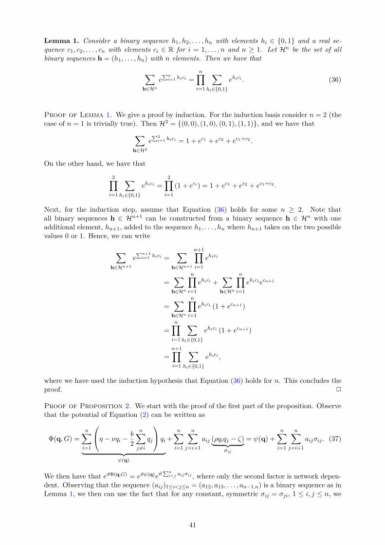
Lemma 1. Consider a binary sequence h1, h2, . . . , hn with elements hi ∈ 0, 1 and a real se-quence c1, c2, . . . , cn with elements ci ∈ R for i = 1, . . . , n and n ≥ 1. Let Hn be the set of allbinary sequences h = (h1, . . . , hn) with n elements. Then we have that
∑h∈Hn
e∑n
i=1 hici =
n∏i=1
∑hi∈0,1
ehici . (36)
Proof of Lemma 1. We give a proof by induction. For the induction basis consider n = 2 (thecase of n = 1 is trivially true). Then H2 = (0, 0), (1, 0), (0, 1), (1, 1), and we have that∑
h∈H2
e∑2
i=1 hici = 1 + ec1 + ec2 + ec1+c2 .
On the other hand, we have that
2∏i=1
∑hi∈0,1
ehici =
2∏i=1
(1 + eci) = 1 + ec1 + ec2 + ec1+c2 .
Next, for the induction step, assume that Equation (36) holds for some n ≥ 2. Note thatall binary sequences h ∈ Hn+1 can be constructed from a binary sequence h ∈ Hn with oneadditional element, hn+1, added to the sequence h1, . . . , hn where hn+1 takes on the two possiblevalues 0 or 1. Hence, we can write
∑h∈Hn+1
e∑n+1
i=1 hici =∑
h∈Hn+1
n+1∏i=1
ehici
=∑h∈Hn
n∏i=1
ehici +∑h∈Hn
n∏i=1
ehiciecn+1
=∑h∈Hn
n∏i=1
ehici (1 + ecn+1)
=n∏i=1
∑hi∈0,1
ehici (1 + ecn+1)
=n+1∏i=1
∑hi∈0,1
ehici ,
where we have used the induction hypothesis that Equation (36) holds for n. This concludes theproof. 2
Proof of Proposition 2. We start with the proof of the first part of the proposition. Observethat the potential of Equation (2) can be written as
Φ(q, G) =n∑i=1
η − νqi −b
2
n∑j =i
qj
qi︸ ︷︷ ︸ψ(q)
+n∑i=1
n∑j=i+1
aij (ρqiqj − ζ)︸ ︷︷ ︸σij
= ψ(q) +n∑i=1
n∑j=i+1
aijσij . (37)
We then have that eϑΦ(q,G) = eϑψ(q)eϑ∑n
i<j aijσij , where only the second factor is network depen-dent. Observing that the sequence (aij)1≤i<j≤n = (a12, a13, . . . , an−1,n) is a binary sequence as inLemma 1, we then can use the fact that for any constant, symmetric σij = σji, 1 ≤ i, j ≤ n, we
41
can write51 ∑G∈Gn
eϑ∑n
i<j aijσij =n∏i=1
n∏j=i+1
(1 + eϑσij
). (38)
From Equation (38) we then obtain
∑G∈Gn
eϑΦ(q,G) = eϑψ(q)n∏i<j
(1 + eϑσij
)=
n∏i=1
eϑ(ηi−νqi−b2
∑nj =i qj)qi
n∏i<j
(1 + eϑ(ρqiqj−ζ)
). (39)
We can use Equation (39) to compute the marginal distribution
µϑ(q) =1
Zϑ
∑G∈Gn
eϑΦ(q,G)
=1
Zϑ
n∏i=1
eϑ(ηi−νqi−b2
∑j =i qj)qi
n∏i<j
(1 + eϑ(ρqiqj−ζ)
)=
1
Zϑeϑ
∑ni=1(ηi−νqi−
b2
∑j =i qj)qie
∑ni<j ln
(1+eϑ(ρqiqj−ζ)
)
=1
ZϑeϑHϑ(q), (40)
where we have introduced the Hamiltonian
Hϑ(q) ≡n∑i=1
ηqi − νq2i +n∑j>i
(1
ϑln(1 + eϑ(ρqiqj−ζ)
)− bqiqj
) . (41)
Using the fact that∫Qn µ
ϑ(q)dq = 1, it follows from Equation (40) that we can write the partitionfunction as
Zϑ =
∫Qn
eϑHϑ(q)dq.
We next make the Laplace approximation [Wong, 2001, Theorem 3, p. 495]
Zϑ ∼(2π
ϑ
)n2
∣∣∣∣∣(∂2Hϑ
∂qi∂qj
)qi=q∗
∣∣∣∣∣− 1
2
eϑHϑ(q∗), (42)
for large ϑ, where q∗ = argmaxq∈[0,q]n Hϑ(q), and the Hessian is given by ∂2Hϑ∂qi∂qj
for 1 ≤ i, j ≤ n.From Equation (41) we find that
∂Hϑ
∂qi= η − 2νqi +
n∑j =i
(ρ
2
(1 + tanh
(ϑ
2(ρqiqj − ζ)
))− b
)qj . (43)
The first order conditions ∂Hϑ∂qi
= 0 in Equation (43) imply that
η − 2νqi =
n∑j =i
(b− ρ
2
(1 + tanh
(ϑ
2(ρqiqj − ζ)
)))qj .
51Note that Equation (38) requires the σij to be constant, and in particular, to be independent. In this case thesummation over all networks only needs to count the number of possible networks in which the link ij is present.In contrast, when σij depends on the other links in the network, then this simple summation formula would nolonger hold.
42
This system of equations has a symmetric solution, qi = q for all i = 1, . . . , n, where
(b(n− 1) + 2ν)q − η =(n− 1)ρ
2
(1 + tanh
(ϑ
2
(ρq2 − ζ
)))q.
Introducing the variables η∗ ≡ η/(n− 1) and ν∗ ≡ ν/(n− 1), this can be written as
(b+ 2ν∗)q − η∗ =ρ
2
(1 + tanh
(ϑ
2
(ρq2 − ζ
)))q. (44)
Let the RHS of Equation (44) be denoted by F (q) so that we can write it as (b + 2ν∗)q − η∗ =F (q). Then we have that F (0) = 0, F ′(q) ≥ 0 and F (q) ∼ ρq for q → ∞. It follows that(b + 2ν∗)q − η∗ = F (q) has at least one solution when b + 2ν∗ > ρ.52 Moreover, any iteration(b + 2ν∗)qt+1 − η∗ = F (qt) starting at q0 = 0 converges to the smallest fixed point q∗ such that(b+ 2ν∗)q∗ − η∗ = F (q∗).
We next compute the average output level q = 1n
∑ni=1 qi. We have that
Eµϑ
(n∑i=1
qi
)=∑G∈Gn
∫Qn
dq
(n∑i=1
qi
)µϑ(q, G) =
1
Zϑ
∑G∈Gn
∫Qn
dq
(n∑i=1
qi
)eϑΦ(q,G)
=1
Zϑ
∑G∈Gn
∫Qn
dq1
ϑ
∂
∂ηeϑΦ(q,G) =
1
ϑ
1
Zϑ
∂Zϑ
∂η=
1
ϑ
∂ lnZϑ
∂η= − 1
ϑ
∂Fϑ
∂η,
where we have denoted by Fϑ ≡ − lnZϑ. The average output is then given by
Eµϑ
(1
n
n∑i=1
qi
)= − 1
nϑ
∂Fϑ
∂η.
With Equation (42) we get
Fϑ ∼ −n2ln
(2π
ϑ
)+
1
2ln
∣∣∣∣∣(∂2Hϑ
∂qi∂qj
)qi=q∗
∣∣∣∣∣− ϑHϑ(q∗).
We then find that
∂Fϑ
∂η= −ϑ∂Hϑ(q
∗)
∂η+
1
2
∂
∂ηln
∣∣∣∣∣(∂2Hϑ
∂qi∂qj
)qi=q∗
∣∣∣∣∣= −ϑ∂Hϑ(q
∗)
∂η+
1
2tr((
∂2Hϑ
∂qi∂qj
)−1∂
∂η
(∂2Hϑ
∂qi∂qj
))qi=q∗
,
where we have used Jacobi’s formula [Horn and Johnson, 1990].53 From Equation (43) we furtherhave that
∂2Hϑ
∂q2i= −2ν +
ϑρ2
4
n∑j =i
q2j
(1− tanh
(ϑ
2(ρqiqj − ζ)
)2), (45)
52Since the RHS, F (q), of Equation (44) is increasing (one can see this from taking the derivative), is zero atq = 0, i.e. F (0) = 0, and asymptotically grows linearly as ρq, it follows that when b+ 2ν∗ > ρ there must exist atleast one fixed point. This is because the LHS, (b+2ν∗)q− η∗, of Equation (44) starts below zero at q = 0 (whereit is −η∗), both LHS and RHS are increasing, and the RHS approaches asymptotically a line with a slope smallerthan the slope b+ 2ν∗ of the LHS. Hence they must intersect at some q ≥ 0.
53For any invertible matrix M(x) for all x, Jacobi’s formula states that ddx
|M(x)| = |M(x)| tr(M(x)−1 d
dxM(x)
),
which can be written more compactly as ddx
ln |M(x)| = tr(M(x)−1 d
dxM(x)
).
43

and for j = i we have that
∂2Hϑ
∂qi∂qj= −b+ ρ
2
(1 + tanh
(ϑ
2(ρqiqj − ζ)
))(1 +
ϑρ
2qiqj
(1− tanh
(ϑ
2(ρqiqj − ζ)
))).
(46)
This shows that ∂∂η
(∂2Hϑ∂qi∂qj
)= 0, so that ∂Fϑ
∂η = −ϑ∂Hϑ(q∗)
∂η , and the expected average outputlevel is then given by
Eµϑ
(1
n
n∑i=1
qi
)=
1
n
∂Hϑ(q∗)
∂η.
Using the fact that ∂Hϑ(q∗)
∂η =∑n
i=1 qi = nq∗, we then get in leading order terms for large ϑ that
Eµ∗(1
n
n∑i=1
qi
)= lim
ϑ→∞Eµϑ
(1
n
n∑i=1
qi
)= q∗.
Next, we compute the output distribution. It can be written as follows
µϑ(q) =1
Zϑ
∑G∈Gn
eϑΦ(q,G) =1
Z ϑn
eϑHϑ(q),
where the Hamiltonian is implicitly defined by eϑHϑ(q) =∑
G∈Gn eϑΦ(q,G). From a Taylor expan-sion around q∗ we have that
Hϑ(q) = Hϑ(q∗) + (q− q∗)∇Hϑ(q
∗) +1
2(q− q∗)⊤∆Hϑ(q
∗)(q− q∗) + o(∥q− q∗∥2
),
as ϑ → ∞, where q∗ = argmaxq∈[0,q]n Hϑ(q), the gradient is ∇Hϑ(q) =(∂Hϑ∂qi
)i=1,...,n
, and the
Hessian is ∆Hϑ(q) =(∂2Hϑ∂qi∂qj
)i,j=1,...,n
. As the gradient ∇Hϑ(q) vanishes at q∗, we have that
Hϑ(q) = Hϑ(q∗) +
1
2(q− q∗)⊤∆Hϑ(q
∗)(q− q∗) + o(∥q− q∗∥2
).
We then can write
µϑ(q) =1
Z ϑn
eϑHϑ(q∗) exp
−1
2ϑ(q− q∗)⊤(−∇Hϑ(q
∗))(q− q∗)
+ o
(∥q− q∗∥2
).
Normalization implies that
Z ϑn =
∫Qn
dqeHϑ(q) = eϑHϑ(q∗)
∫Qn
dq exp
−1
2ϑ(q− q∗)⊤(−∆Hϑ(q
∗))(q− q∗)
+ o
(∥q− q∗∥2
)= eϑHϑ(q
∗)(2π)n2 |−∆Hϑ(q
∗)|−12 + o
(∥q− q∗∥2
).
The Laplace approximation of µϑ(q) is then given by
µϑ(q) =
(2π
ϑ
)−n2
|−∆Hϑ(q∗)|
12 exp
−1
2ϑ(q− q∗)⊤(−∆Hϑ(q
∗))(q− q∗)
+ o
(∥q− q∗∥2
).
(47)That is, in the limit of large ϑ, q is asymptotically normally distributed with mean q∗ andvariance − 1
ϑ∇Hϑ(q∗)−1.
44
Imposing symmetry, qi = q for all i = 1, . . . , n, in Equation (45) we can write
∂2Hϑ
∂q2i
∣∣∣∣qi=q
= −2ν + (n− 1)ϑρ2
4q2(1− tanh
(ϑ
2
(ρq2 − ζ
)))(1 + tanh
(ϑ
2
(ρq2 − ζ
))),
and for j = i we have from Equation (45) that
∂2Hϑ
∂qi∂qj
∣∣∣∣qi=qj=q
= −b+ ρ
2
(1 + tanh
(ϑ
2
(ρq2 − ζ
)))(1 +
ϑρ
2q2(1− tanh
(ϑ
2
(ρq2 − ζ
)))).
Using Equation (44), from which we get
ρ
2
(1 + tanh
(ϑ
2
(ρq2 − ζ
)))=
((n− 1)b+ 2ν)q − η
(n− 1)q,
andρ
2
(1− tanh
(ϑ
2(ρqiqj − ζ)
))=
((n− 1)(ρ− b)− 2ν)q + η
(n− 1)q,
we then can write
∂2Hϑ
∂q2i
∣∣∣∣qi=q
= −2ν +ϑ(((n− 1)(ρ− b)− 2ν)q + η)(((n− 1)b+ 2ν)q − η)
n− 1,
and
∂2Hϑ
∂qi∂qj
∣∣∣∣qi=qj=q
= −b+ ((n− 1)b+ 2ν)q − η
(n− 1)q
(1 +
ϑq(((n− 1)(ρ− b)− 2ν)q + η)
n− 1
).
Denoting by ν∗ ≡ ν/(n− 1) and η∗ ≡ η/(n− 1) we can further write
∂2Hϑ
∂q2i
∣∣∣∣qi=q
= (n− 1)
(−2ν∗ + ϑq2
(ρ− b− 2ν∗ +
η∗
q
)(b+ 2ν∗ − η∗
q
)), (48)
and∂2Hϑ
∂qi∂qj
∣∣∣∣qi=qj=q
= −b+(b+ 2ν∗ − η∗
q
)(1 + ϑq2
(ρ− b− 2ν∗ +
η∗
q
)). (49)
Note that due to symmetry, the Hessian ∆Hϑ(q∗) with components in Equations (48) and
(49) is a special case of a circulant matrix. Denoting by a the diagonal elements of ∆Hϑ(q∗) and
by b the off-diagonal elements, the determinant in Equation (47) follows from the general formula[Horn and Johnson, 1990]:
|−∆Hϑ(q∗)| =
∣∣∣∣∣∣∣∣∣a b b . . .b a b . . .b b a...
... . . .
∣∣∣∣∣∣∣∣∣ = (a− b)n−1(a+ (n− 1)b).
Similarly, for a circulant matrix (by applying the Sherman-Morrison formula ( Horn and Johnson
45

[1990]) we get for the inverse in Equation (47) that
−∆Hϑ(q∗)−1 =
a b b . . .b a b . . .b b a...
... . . .
−1
=1
a2 + (n− 2)ab− (n− 1)b2
a+ (n− 2)b −b −b . . .
−b a+ (n− 2)b −b . . .−b −b a+ (n− 2)b...
... . . .
,
For large n we see from Equations (48) and (49) that the off-diagonal elements vanish relative tothe diagonal elements. As q is asymptotically normally distributed with mean q∗ and variance− 1ϑ∆Hϑ(q
∗)−1, this implies that, in the limit of n → ∞, the individual firms’ output levelsbecome independent. The diagonal entries are given by
− 1
ϑ(∆Hϑ(q
∗))−1ii ∼ 1
ϑ
n
2ν∗ + ϑ(bq − η∗ + 2ν∗q)(q(b+ 2ν∗ − ρ)− η∗)≡ σ2.
Next, we compute the expected average degree d. The expected number of links can be obtainedas follows
Eµϑ(m) =∑G∈Gn
∫Qn
mµϑ(q, G)dq =1
Zϑ
∑G∈Gn
∫Qn
meϑΦ(q,G)︸ ︷︷ ︸− 1
ϑ∂∂ζeϑΦ(q,G)
dq = − 1
ϑ
1
Zϑ
∂Zϑ
∂ζ=
1
ϑ
∂Fϑ
∂ζ,
where we have denoted by Fϑ ≡ − lnZϑ. From the Laplace approximation in Equation (42) wefind that
∂Fϑ
∂ζ= −ϑ∂Hϑ(q
∗)
∂ζ+
1
2
∂
∂ζln
∣∣∣∣∣(∂2Hϑ
∂qi∂qj
)qi=q∗
∣∣∣∣∣= −ϑ∂Hϑ(q
∗)
∂ζ+
1
2tr((
∂2Hϑ
∂qi∂qj
)−1∂
∂ζ
(∂2Hϑ
∂qi∂qj
))qi=q∗
,
where we have used Jacobi’s formula [see e.g. Horn and Johnson, 1990]. Consequently, theexpected number of links is
Eµϑ(m) = −∂Hϑ(q∗)
∂ζ+
1
2ϑtr((
∂2Hϑ
∂qi∂qj
)−1∂
∂ζ
(∂2Hϑ
∂qi∂qj
))qi=q∗
.
Further, we have that
∂Hϑ
∂ζ= −1
2
n∑i=1
n∑j>i
(1 + tanh
(ϑ
2(ρqiqj − ζ)
)),
and in the symmetric equilibrium this is
∂Hϑ
∂ζ
∣∣∣∣qi=q
= −n(n− 1)
4
(1 + tanh
(ϑ
2
(ρq2 − ζ
))).
The expected number of links can then be written as
Eµϑ(m) =n(n− 1)
2
(1 + tanh
(ϑ
2
(ρq2 − ζ
)))+
1
2ϑtr((
∂2Hϑ
∂qi∂qj
)−1∂
∂ζ
(∂2Hϑ
∂qi∂qj
))qi=q∗
.
46

Using the fact thatρ
2
(1 + tanh
(ϑ
2
(ρq2 − ζ
))2)
= b+ 2ν∗ − η∗
q,
where ν∗ = νn−1 and η∗ = η
n−1 , we can write
∂Hϑ
∂ζ
∣∣∣∣qi=q
= −n(n− 1)
2ρ
(b+ 2ν∗ − η∗
q
).
In the limit of ϑ → ∞ in the low equilibrium, where q = η∗
b+2ν∗ and therefore η∗
q = b + 2ν∗, wethen get
∂Hϑ
∂ζ
∣∣∣∣qi=q
= 0.
In contrast, in the limit of ϑ→ ∞ in the high equilibrium, where q = η∗
b+2ν∗−ρ , and η∗
q = b+2ν∗−ρwe find that
∂Hϑ
∂ζ
∣∣∣∣qi=q
= −n(n− 1)
2.
Further, the derivatives with respect to ζ in Equation (45) are given by
∂
∂ζ
∂2Hϑ
∂q2i=ϑ2ρ2
4
n∑j =i
tanh
(ϑ
2(ρqiqj − ζ)
)(1− tanh
(ϑ
2(ρqiqj − ζ)
)2),
and for j = i from Equation (46) we get that
∂
∂ζ
∂2Hϑ
∂qi∂qj= −ϑρ
4
(1− tanh
(ϑ
2(ρqiqj − ζ)
)2)(
1− ϑρqiqj tanh
(ϑ
2(ρqiqj − ζ)
)).
Imposing symmetry, qi = q for all i = 1, . . . , n, we then can write
∂
∂ζ
∂2Hϑ
∂q2i
∣∣∣∣qi=q
=(n− 1)ϑ2ρ2
4tanh
(ϑ
2
(ρq2 − ζ
))(1− tanh
(ϑ
2
(ρq2 − ζ
))2), (50)
and
∂
∂ζ
∂2Hϑ
∂qi∂qj
∣∣∣∣qi=qj=q
= −ϑρ4
(1− tanh
(ϑ
2
(ρq2 − ζ
))2)(
1− ϑρq2 tanh
(ϑ
2
(ρq2 − ζ
))). (51)
For a circulant matrix (by applying the Sherman-Morrison formula [Horn and Johnson, 1990] wehave thata b b . . .b a b . . .b b a...
... . . .
−1
=1
a2 + (n− 2)ab− (n− 1)b2
a+ (n− 2)b −b −b . . .
−b a+ (n− 2)b −b . . .−b −b a+ (n− 2)b...
... . . .
,
and
tr
c d d . . .d c d . . .d d c...
... . . .
e f f . . .f e f . . .f f e...
... . . .
= n(ce+ (n− 1)df),
47
so that
tr
a b b . . .b a b . . .b b a...
... . . .
−1
e f f . . .f e f . . .f f e...
... . . .
=n((a+ (n− 2)b)e− (n− 1)bf)
a2 + (n− 2)ab− (n− 1)b2.
The expected number of links can then be written as follows
Eµϑ(m) =n(n− 1)
2
(1 + tanh
(ϑ
2
(ρq2 − ζ
)))+
1
2ϑRϑ,
whereRϑ ≡ n((c1 + (n− 2)c2)c3 − (n− 1)c2c4)
c21 + (n− 2)c1c2 − (n− 1)c22,
with
c1 ≡ −2ν + (n− 1)ϑρ2q2
4
(1− tanh
(ϑ
2
(ρq2 − ζ
))2),
c2 ≡ −b+ ρ
2
(1 + tanh
(ϑ
2
(ρq2 − ζ
)))(1 +
ϑρq2
2
(1− tanh
(ϑ
2
(ρq2 − ζ
)))),
c3 ≡(n− 1)ϑ2ρ2
4tanh
(1− tanh
(ϑ
2
(ρq2 − ζ
))2),
c4 ≡ −ρϑ4
(1− tanh
(ϑ
2
(ρq2 − ζ
))2)(
1− ϑρq2 tanh
(ϑ
2
(ρq2 − ζ
))).
In the following we compute the degree distribution. From our previous discussion we know thateach firm i has an output level q distributed identically and independently with density µϑ(q) givenby N (q∗, σ2) and converging to δ(q−q∗) in the limit ϑ→ ∞. With the marginal distribution fromEquation (40) and the potential in Equation (37) we then can write the conditional distributionas
µϑ(G|q) = µϑ(q, G)
µϑ(q)=
eϑΦ(q,G)∑G′∈Gn eϑΦ(q,G′)
=eψ(q)eϑ
∑ni<j aij(ρqiqj−ζ)
eψ(q)∏i<j
(1 + eϑ(ρqiqj−ζ)
)=
eϑ∑n
i<j aij(ρqiqj−ζ)∏i<j
(1 + eϑ(ρqiqj−ζ)
)=∏i<j
eϑaij(ρqiqj−ζ)
1 + eϑ(ρqiqj−ζ)
=∏i<j
(eϑ(ρqiqj−ζ)
1 + eϑ(ρqiqj−ζ)
)aij (1− eϑ(ρqiqj−ζ)
1 + eϑ(ρqiqj−ζ)
)1−aij
=∏i<j
pϑ(qi, qj)aij(1− pϑ(qi, qj)
)1−aij. (52)
Hence, we obtain the likelihood of an inhomogeneous random graph with link probability54
pϑ(qi, qj) =eϑ(ρqiqj−ζ)
1 + eϑ(ρqiqj−ζ)=
gϑ(qi, qj)
1 + gϑ(qi, qj), (53)
where we have denoted by gϑ(q, q′) ≡ eϑ(ρqq′−ζ). The probability of observing the network G,
54See also supplementary Appendix B, Boguná and Pastor-Satorras [2003] and and Söderberg [2002].
48
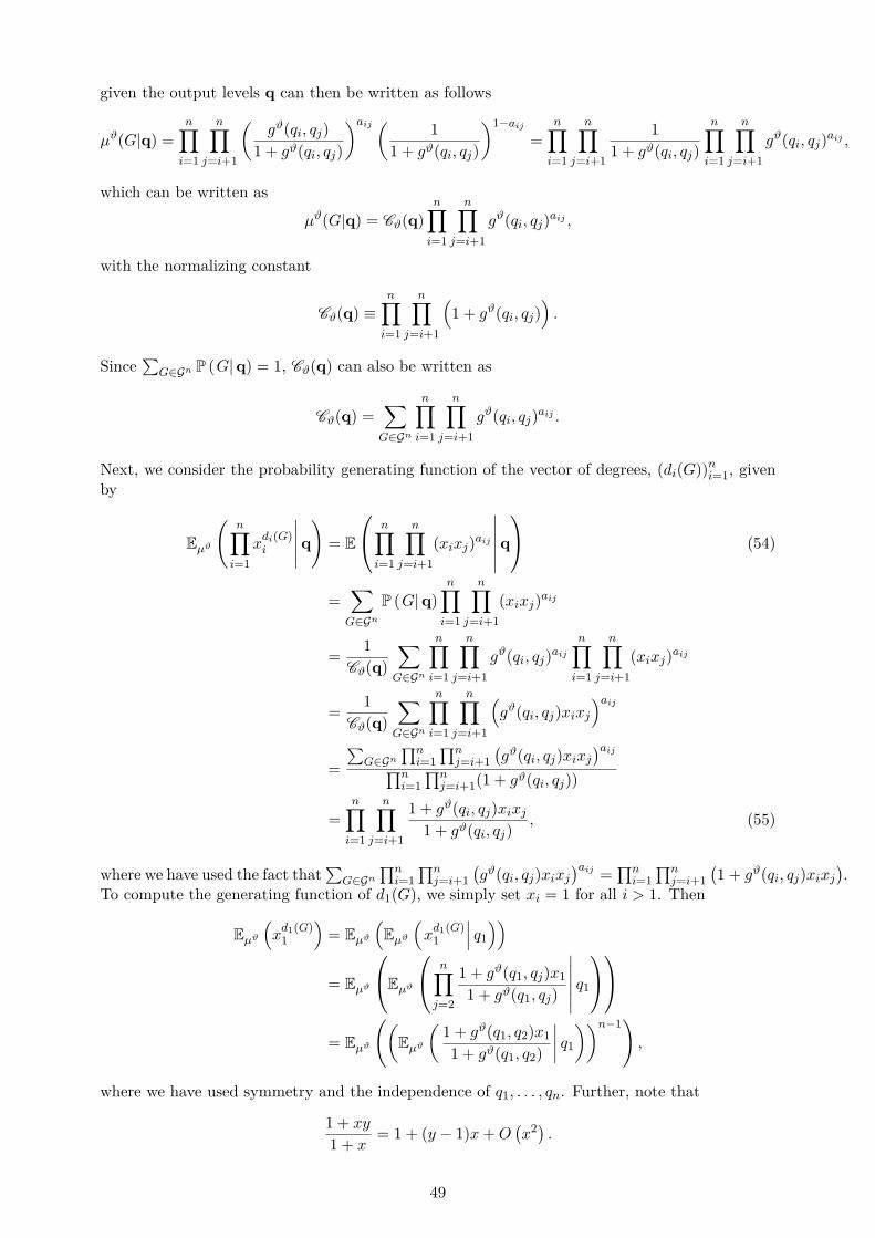
given the output levels q can then be written as follows
µϑ(G|q) =n∏i=1
n∏j=i+1
(gϑ(qi, qj)
1 + gϑ(qi, qj)
)aij ( 1
1 + gϑ(qi, qj)
)1−aij=
n∏i=1
n∏j=i+1
1
1 + gϑ(qi, qj)
n∏i=1
n∏j=i+1
gϑ(qi, qj)aij ,
which can be written asµϑ(G|q) = Cϑ(q)
n∏i=1
n∏j=i+1
gϑ(qi, qj)aij ,
with the normalizing constant
Cϑ(q) ≡n∏i=1
n∏j=i+1
(1 + gϑ(qi, qj)
).
Since∑
G∈Gn P (G|q) = 1, Cϑ(q) can also be written as
Cϑ(q) =∑G∈Gn
n∏i=1
n∏j=i+1
gϑ(qi, qj)aij .
Next, we consider the probability generating function of the vector of degrees, (di(G))ni=1, givenby
Eµϑ
(n∏i=1
xdi(G)i
∣∣∣∣∣q)
= E
n∏i=1
n∏j=i+1
(xixj)aij
∣∣∣∣∣∣q (54)
=∑G∈Gn
P (G|q)n∏i=1
n∏j=i+1
(xixj)aij
=1
Cϑ(q)
∑G∈Gn
n∏i=1
n∏j=i+1
gϑ(qi, qj)aij
n∏i=1
n∏j=i+1
(xixj)aij
=1
Cϑ(q)
∑G∈Gn
n∏i=1
n∏j=i+1
(gϑ(qi, qj)xixj
)aij=
∑G∈Gn
∏ni=1
∏nj=i+1
(gϑ(qi, qj)xixj
)aij∏ni=1
∏nj=i+1(1 + gϑ(qi, qj))
=n∏i=1
n∏j=i+1
1 + gϑ(qi, qj)xixj1 + gϑ(qi, qj)
, (55)
where we have used the fact that∑
G∈Gn
∏ni=1
∏nj=i+1
(gϑ(qi, qj)xixj
)aij =∏ni=1
∏nj=i+1
(1 + gϑ(qi, qj)xixj
).
To compute the generating function of d1(G), we simply set xi = 1 for all i > 1. Then
Eµϑ(xd1(G)1
)= Eµϑ
(Eµϑ
(xd1(G)1
∣∣∣ q1))= Eµϑ
Eµϑ
n∏j=2
1 + gϑ(q1, qj)x11 + gϑ(q1, qj)
∣∣∣∣∣∣ q1
= Eµϑ
((Eµϑ
(1 + gϑ(q1, q2)x11 + gϑ(q1, q2)
∣∣∣∣ q1))n−1),
where we have used symmetry and the independence of q1, . . . , qn. Further, note that
1 + xy
1 + x= 1 + (y − 1)x+O
(x2).
49
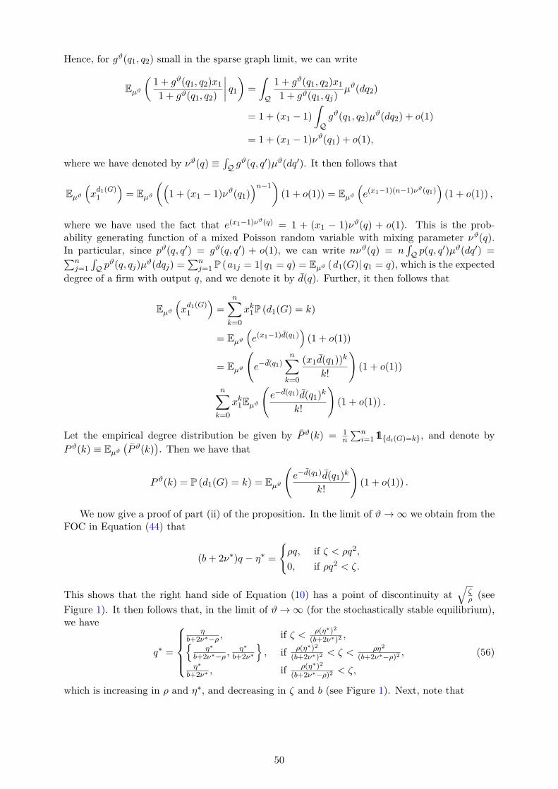
Hence, for gϑ(q1, q2) small in the sparse graph limit, we can write
Eµϑ(1 + gϑ(q1, q2)x11 + gϑ(q1, q2)
∣∣∣∣ q1) =
∫Q
1 + gϑ(q1, q2)x11 + gϑ(q1, qj)
µϑ(dq2)
= 1 + (x1 − 1)
∫Qgϑ(q1, q2)µ
ϑ(dq2) + o(1)
= 1 + (x1 − 1)νϑ(q1) + o(1),
where we have denoted by νϑ(q) ≡∫Q g
ϑ(q, q′)µϑ(dq′). It then follows that
Eµϑ(xd1(G)1
)= Eµϑ
((1 + (x1 − 1)νϑ(q1)
)n−1)(1 + o(1)) = Eµϑ
(e(x1−1)(n−1)νϑ(q1)
)(1 + o(1)) ,
where we have used the fact that e(x1−1)νϑ(q) = 1 + (x1 − 1)νϑ(q) + o(1). This is the prob-ability generating function of a mixed Poisson random variable with mixing parameter νϑ(q).In particular, since pϑ(q, q′) = gϑ(q, q′) + o(1), we can write nνϑ(q) = n
∫Q p(q, q
′)µϑ(dq′) =∑nj=1
∫Q p
ϑ(q, qj)µϑ(dqj) =
∑nj=1 P (a1j = 1| q1 = q) = Eµϑ (d1(G)| q1 = q), which is the expected
degree of a firm with output q, and we denote it by d(q). Further, it then follows that
Eµϑ(xd1(G)1
)=
n∑k=0
xk1P (d1(G) = k)
= Eµϑ(e(x1−1)d(q1)
)(1 + o(1))
= Eµϑ
(e−d(q1)
n∑k=0
(x1d(q1))k
k!
)(1 + o(1))
n∑k=0
xk1Eµϑ
(e−d(q1)d(q1)
k
k!
)(1 + o(1)) .
Let the empirical degree distribution be given by P ϑ(k) = 1n
∑ni=1 1di(G)=k, and denote by
P ϑ(k) ≡ Eµϑ(P ϑ(k)
). Then we have that
P ϑ(k) = P (d1(G) = k) = Eµϑ
(e−d(q1)d(q1)
k
k!
)(1 + o(1)) .
We now give a proof of part (ii) of the proposition. In the limit of ϑ→ ∞ we obtain from theFOC in Equation (44) that
(b+ 2ν∗)q − η∗ =
ρq, if ζ < ρq2,
0, if ρq2 < ζ.
This shows that the right hand side of Equation (10) has a point of discontinuity at√
ζρ (see
Figure 1). It then follows that, in the limit of ϑ→ ∞ (for the stochastically stable equilibrium),we have
q∗ =
η
b+2ν∗−ρ , if ζ < ρ(η∗)2
(b+2ν∗)2 ,η∗
b+2ν∗−ρ ,η∗
b+2ν∗
, if ρ(η∗)2
(b+2ν∗)2 < ζ < ρη2
(b+2ν∗−ρ)2 ,
η∗
b+2ν∗ , if ρ(η∗)2
(b+2ν∗−ρ)2 < ζ,
(56)
which is increasing in ρ and η∗, and decreasing in ζ and b (see Figure 1). Next, note that
50
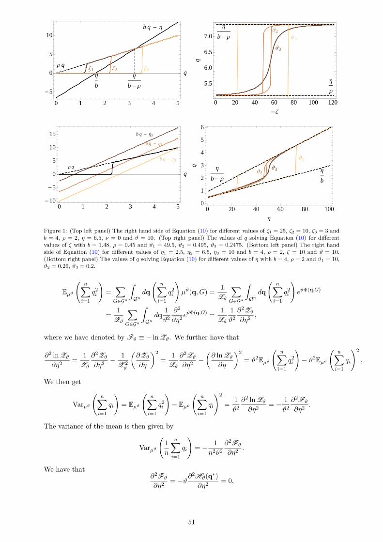
b q - Η
Ρ q
Η
b
Η
b- Ρ
Ζ1 Ζ2 Ζ3
0 1 2 3 4 5
-5
0
5
10
q
Η
b- Ρ
Η
Ρ
J3
J2
J1
0 20 40 60 80 100 120
5.5
6.0
6.5
7.0
-Ζ
q
b q - Η3
b q - Η2
b q - Η1
Ρ q
0 1 2 3 4 5-10
-5
0
5
10
15
qΗ
b- ΡΗ
b
J1
J3J2
0 20 40 60 80 1000
1
2
3
4
5
6
Η
q
Figure 1: (Top left panel) The right hand side of Equation (10) for different values of ζ1 = 25, ζ2 = 10, ζ3 = 3 andb = 4, ρ = 2, η = 6.5, ν = 0 and ϑ = 10. (Top right panel) The values of q solving Equation (10) for differentvalues of ζ with b = 1.48, ρ = 0.45 and ϑ1 = 49.5, ϑ2 = 0.495, ϑ3 = 0.2475. (Bottom left panel) The right handside of Equation (10) for different values of η1 = 2.5, η2 = 6.5, η3 = 10 and b = 4, ρ = 2, ζ = 10 and ϑ = 10.(Bottom right panel) The values of q solving Equation (10) for different values of η with b = 4, ρ = 2 and ϑ1 = 10,ϑ2 = 0.26, ϑ3 = 0.2.
Eµϑ
(n∑i=1
q2i
)=∑G∈Gn
∫Qn
dq
(n∑i=1
q2i
)µϑ(q, G) =
1
Zϑ
∑G∈Gn
∫Qn
dq
(n∑i=1
q2i
)eϑΦ(q,G)
=1
Zϑ
∑G∈Gn
∫Qn
dq1
ϑ2∂2
∂η2eϑΦ(q,G) =
1
Zϑ
1
ϑ2∂2Zϑ
∂η2,
where we have denoted by Fϑ ≡ − lnZϑ. We further have that
∂2 lnZϑ
∂η2=
1
Zϑ
∂2Zϑ
∂η2− 1
Z 2ϑ
(∂Zϑ
∂η
)2
=1
Zϑ
∂2Zϑ
∂η2−(∂ lnZϑ
∂η
)2
= ϑ2Eµϑ
(n∑i=1
q2i
)− ϑ2Eµϑ
(n∑i=1
qi
)2
.
We then get
Varµϑ
(n∑i=1
qi
)= Eµϑ
(n∑i=1
q2i
)− Eµϑ
(n∑i=1
qi
)2
=1
ϑ2∂2 lnZϑ
∂η2= − 1
ϑ2∂2Fϑ
∂η2.
The variance of the mean is then given by
Varµϑ
(1
n
n∑i=1
qi
)= − 1
n2ϑ2∂2Fϑ
∂η2.
We have that∂2Fϑ
∂η2= −ϑ∂
2Hϑ(q∗)
∂η2= 0,
51
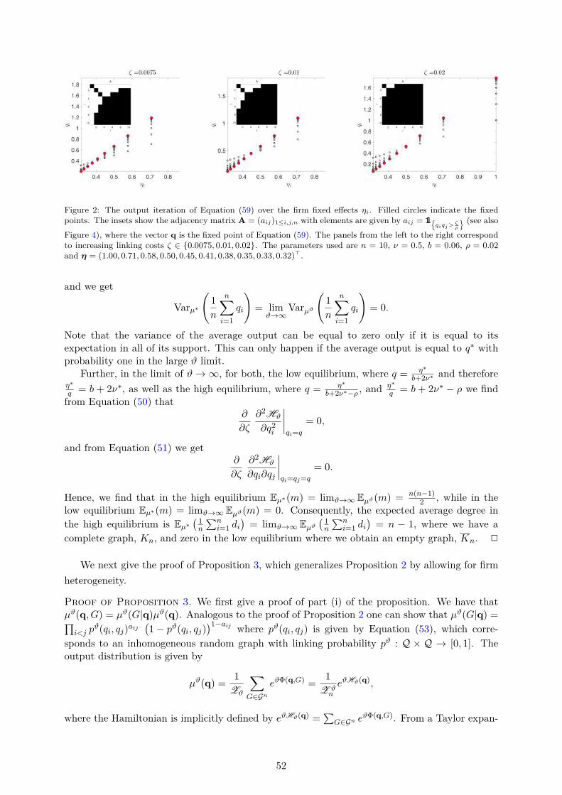
Figure 2: The output iteration of Equation (59) over the firm fixed effects ηi. Filled circles indicate the fixedpoints. The insets show the adjacency matrix A = (aij)1≤i,j,n with elements are given by aij = 1
qiqj>ζρ
(see alsoFigure 4), where the vector q is the fixed point of Equation (59). The panels from the left to the right correspondto increasing linking costs ζ ∈ 0.0075, 0.01, 0.02. The parameters used are n = 10, ν = 0.5, b = 0.06, ρ = 0.02and η = (1.00, 0.71, 0.58, 0.50, 0.45, 0.41, 0.38, 0.35, 0.33, 0.32)⊤.
and we get
Varµ∗
(1
n
n∑i=1
qi
)= lim
ϑ→∞Varµϑ
(1
n
n∑i=1
qi
)= 0.
Note that the variance of the average output can be equal to zero only if it is equal to itsexpectation in all of its support. This can only happen if the average output is equal to q∗ withprobability one in the large ϑ limit.
Further, in the limit of ϑ→ ∞, for both, the low equilibrium, where q = η∗
b+2ν∗ and thereforeη∗
q = b + 2ν∗, as well as the high equilibrium, where q = η∗
b+2ν∗−ρ , and η∗
q = b + 2ν∗ − ρ we findfrom Equation (50) that
∂
∂ζ
∂2Hϑ
∂q2i
∣∣∣∣qi=q
= 0,
and from Equation (51) we get∂
∂ζ
∂2Hϑ
∂qi∂qj
∣∣∣∣qi=qj=q
= 0.
Hence, we find that in the high equilibrium Eµ∗(m) = limϑ→∞ Eµϑ(m) = n(n−1)2 , while in the
low equilibrium Eµ∗(m) = limϑ→∞ Eµϑ(m) = 0. Consequently, the expected average degree inthe high equilibrium is Eµ∗
(1n
∑ni=1 di
)= limϑ→∞ Eµϑ
(1n
∑ni=1 di
)= n − 1, where we have a
complete graph, Kn, and zero in the low equilibrium where we obtain an empty graph, Kn. 2
We next give the proof of Proposition 3, which generalizes Proposition 2 by allowing for firmheterogeneity.
Proof of Proposition 3. We first give a proof of part (i) of the proposition. We have thatµϑ(q, G) = µϑ(G|q)µϑ(q). Analogous to the proof of Proposition 2 one can show that µϑ(G|q) =∏i<j p
ϑ(qi, qj)aij(1− pϑ(qi, qj)
)1−aij where pϑ(qi, qj) is given by Equation (53), which corre-sponds to an inhomogeneous random graph with linking probability pϑ : Q × Q → [0, 1]. Theoutput distribution is given by
µϑ(q) =1
Zϑ
∑G∈Gn
eϑΦ(q,G) =1
Z ϑn
eϑHϑ(q),
where the Hamiltonian is implicitly defined by eϑHϑ(q) =∑
G∈Gn eϑΦ(q,G). From a Taylor expan-
52
sion around q∗ (for large ϑ) we have that
Hϑ(q) = Hϑ(q∗) + (q− q∗)∇Hϑ(q
∗) +1
2(q− q∗)⊤∆Hϑ(q
∗)(q− q∗) + o(∥q− q∗∥2
),
as ϑ → ∞, where q∗ = argmaxq∈[0,q]n Hϑ(q), the gradient is ∇Hϑ(q) =(∂Hϑ∂qi
)i=1,...,n
, and the
Hessian is ∆Hϑ(q) =(∂2Hϑ∂qi∂qj
)i,j=1,...,n
. As the gradient ∇Hϑ(q) vanishes at q∗, we have that
Hϑ(q) = Hϑ(q∗) +
1
2(q− q∗)⊤∆Hϑ(q
∗)(q− q∗) + o(∥q− q∗∥2
).
We then can write
µϑ(q) =1
Z ϑn
eϑHϑ(q∗) exp
−1
2ϑ(q− q∗)⊤(−∇Hϑ(q
∗))(q− q∗)
+ o
(∥q− q∗∥2
).
Normalization,∫Qn µ
ϑ(q)dq = 1, implies that
Z ϑn =
∫Qn
eHϑ(q)dq = eϑHϑ(q∗)
∫Qn
exp
−1
2ϑ(q− q∗)⊤(−∆Hϑ(q
∗))(q− q∗)
dq+ o
(∥q− q∗∥2
)= eϑHϑ(q
∗)(2π)n2 |−∆Hϑ(q
∗)|−12 + o
(∥q− q∗∥2
).
The Laplace approximation of µϑ(q) is then given by [Wong, 2001, Theorem 3, p. 495]
µϑ(q) =
(2π
ϑ
)−n2
|−∆Hϑ(q∗)|
12 exp
−1
2ϑ(q− q∗)⊤(−∆Hϑ(q
∗))(q− q∗)
+ o
(∥q− q∗∥2
).
That is, in the limit of large ϑ, q is asymptotically normally distributed with mean q∗ andvariance − 1
ϑδHϑ(q∗)−1, where ∆Hϑ(q) =
(∂2Hϑ∂qi∂qj
)i,j=1,...,n
with ∂2Hϑ
∂q2igiven by Equation (45)
while, for any i = j, ∂2Hϑ∂qi∂qj
is given by Equation (46).We next turn to part (ii) of the proposition. We show that the networks G in the support of
the stationary distribution µϑ(q, G) in the limit of vanishing noise ϑ→ ∞ is a nested split graph.A graph G is a nested split graph if for every node i ∈ N there exist a weight xi and a thresholdT such that vertices i and j are linked if and only if xi + xj ≥ T [Mahadev and Peled, 1995].
In the limit ϑ→ ∞ the conditional probability of the network G can be written as µ∗(G|q) =limϑ→∞ µϑ(G|q) =
∏ni<j 1
aijρqiqj>ζ1
1−aijρqiqj<ζ. Assume that G is a stochastically stable network,
that is for G ∈ Ω∗, we must have that µ∗(q, G) = limϑ→∞ µϑ(q, G) > 0. Since, µ∗(q, G) =µ∗(G|q)µ∗(q) this implies that µ∗(G|q) > 0. It follows that ρqiqj > ζ for all aij = 1 andρqiqj < ζ for all aij = 0. We then define the weights xi ≡ log qi, xj ≡ log qj and a thresholdT ≡ log ζ − log ρ, and conclude that G is a nested split graph (or threshold graph, see alsosupplementary Appendix B).
Moreover, the output distribution is given by µϑ(q) = 1Zϑ
∑G∈Gn eϑΦ(q,G) = 1
Z ϑneϑHϑ(q), where
the Hamiltonian is given by Equation (41). The output profile that maximizes the Hamiltoniancan be found from the FOC , ∂Hϑ
∂qi= 0, from which we get
qi =ηi2ν
+1
2ν
n∑j =i
(ρ
2
(1 + tanh
(ϑ
2(ρqiqj − ζ)
))− b
)qj .
Taking the limit ϑ→ ∞ and noting that
limϑ→∞
1
2
(1 + tanh
(ϑ
2(ρqiqj − ζ)
))=
1, if ρqiqj > ζ,
0, if ρqiqj < ζ,
53
we thus obtain55
qi =ηi2ν
+1
2ν
n∑j =i
qj
(ρ1
qiqj>ζρ
− b
). (57)
Note that for any profile of output levels q there exists a unique nested split graph with adjacencymatrix A = (aij)1≤i,j,n whose elements are given by aij = 1
qiqj>ζρ
. Then we can write Equation
(57) as follows
qi =ηi2ν
+ρ
2ν
n∑j =i
aijqj −b
2ν
n∑j =i
qj . (58)
Moreover, assume that ηi > ηj , then we want to show that qj > qi for the output profile qsolving Equation (57). For this purpose we consider the iteration
qi,t+1 = fi(qt) ≡ max
0,ηi2ν
+ρ
2ν
n∑j =i
qj,t1qi,tqj,t>
ζρ
− b
2ν
n∑j =i
qj
, (59)
starting from the initial vector q0 = (0, . . . , 0)⊤. We then observe that the map fi : R+ → R+ isη-order preserving. That is, if ηi > ηj and qi,t > qj,t, then also qi,t+1 > qj,t+1. To show this weproceed by induction. For the induction basis consider t = 0. Then qi,1 = ηi for all i = 1, . . . , n,and the claim follows. Next, consider the induction step, assuming that the claim holds for somet > 0. Then
qi,t+1 − qj,t+1 = fi(qt)− fj(qt) =b
2ν(ηi − ηj) +
ρ
2ν
∑k∈Ni,t\Nj,t
qk,t +b
2ν(qi,t − qj,t) > 0,
where we have used the fact that the condition qi,tqj,t >ζρ for i and j being linked represents a
nested split graph, and for such a graph if qi,t > qj,t (so that di,t > dj,t) then Nj,t ⊂ Ni,t. Hence,for all t, the claim holds, and in particular, taking the limit as t→ ∞ it holds for the fixed pointq solving Equation (57).
We now give a proof of part (iii) of the proposition. From Equation (17) we know that in thestochastically stable state the output levels satisfy the following equation
g(q) ≡ (In + bB− ρA)q = η, (60)
where B is a matrix of ones with zero diagonal and A has elements aij = 1ρqiqj>ζ. When the(ηi)
ni=1 are real valued random variables with probability density function f , then the probability
density function µ of q is given by
µ(q) =
∣∣∣∣det(dg(q))dq
)∣∣∣∣ f(η),where
(dg(q)dq
)ij= ∂gi(q)
∂qi. From Equation (60) we get dg(q)
dq = In + bB− ρA, and we denote thisby M. It then follows that µ(q) = | det(M)|f(Mq). In particular, if the (ηi)
ni=1 are identically
and independently Pareto distributed with density function f(η) = (γ − 1)η−γ for η ≥ 1 then
µ(q) = (γ − 1)n|det(M)|n∏i=1
(Mq)−γi .
Next, consider q = cu, c > 0, with u being a vector of all ones. Then M = In+(b−ρ)B for clarge enough (because ρqiqj = c2ρ > ζ for c large enough), and det(M) = (1 + (n− 1)(b− ρ)) (1+
55Note that Hϑ(q) is a real valued function that converges pointwise and whose derivatives converge uniformlyon a closed interval [0, q] so that we can exchange the derivative with the limit [Rudin, 1987].
54
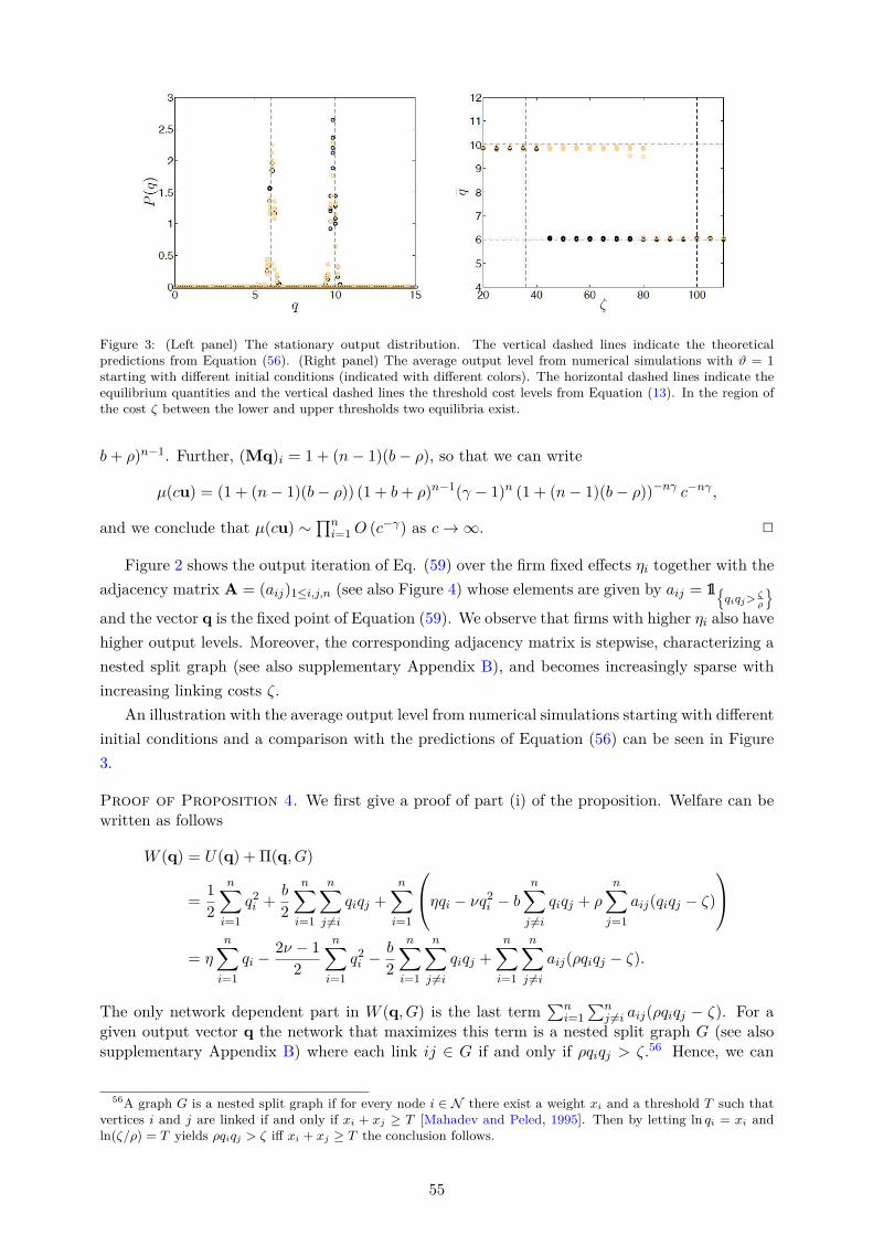
Figure 3: (Left panel) The stationary output distribution. The vertical dashed lines indicate the theoreticalpredictions from Equation (56). (Right panel) The average output level from numerical simulations with ϑ = 1starting with different initial conditions (indicated with different colors). The horizontal dashed lines indicate theequilibrium quantities and the vertical dashed lines the threshold cost levels from Equation (13). In the region ofthe cost ζ between the lower and upper thresholds two equilibria exist.
b+ ρ)n−1. Further, (Mq)i = 1 + (n− 1)(b− ρ), so that we can write
µ(cu) = (1 + (n− 1)(b− ρ)) (1 + b+ ρ)n−1(γ − 1)n (1 + (n− 1)(b− ρ))−nγ c−nγ ,
and we conclude that µ(cu) ∼∏ni=1O (c−γ) as c→ ∞. 2
Figure 2 shows the output iteration of Eq. (59) over the firm fixed effects ηi together with theadjacency matrix A = (aij)1≤i,j,n (see also Figure 4) whose elements are given by aij = 1
qiqj>ζρ
and the vector q is the fixed point of Equation (59). We observe that firms with higher ηi also havehigher output levels. Moreover, the corresponding adjacency matrix is stepwise, characterizing anested split graph (see also supplementary Appendix B), and becomes increasingly sparse withincreasing linking costs ζ.
An illustration with the average output level from numerical simulations starting with differentinitial conditions and a comparison with the predictions of Equation (56) can be seen in Figure3.
Proof of Proposition 4. We first give a proof of part (i) of the proposition. Welfare can bewritten as follows
W (q) = U(q) + Π(q, G)
=1
2
n∑i=1
q2i +b
2
n∑i=1
n∑j =i
qiqj +n∑i=1
ηqi − νq2i − bn∑j =i
qiqj + ρn∑j=1
aij(qiqj − ζ)
= η
n∑i=1
qi −2ν − 1
2
n∑i=1
q2i −b
2
n∑i=1
n∑j =i
qiqj +n∑i=1
n∑j =i
aij(ρqiqj − ζ).
The only network dependent part in W (q, G) is the last term∑n
i=1
∑nj =i aij(ρqiqj − ζ). For a
given output vector q the network that maximizes this term is a nested split graph G (see alsosupplementary Appendix B) where each link ij ∈ G if and only if ρqiqj > ζ.56 Hence, we can
56A graph G is a nested split graph if for every node i ∈ N there exist a weight xi and a threshold T such thatvertices i and j are linked if and only if xi + xj ≥ T [Mahadev and Peled, 1995]. Then by letting ln qi = xi andln(ζ/ρ) = T yields ρqiqj > ζ iff xi + xj ≥ T the conclusion follows.
55
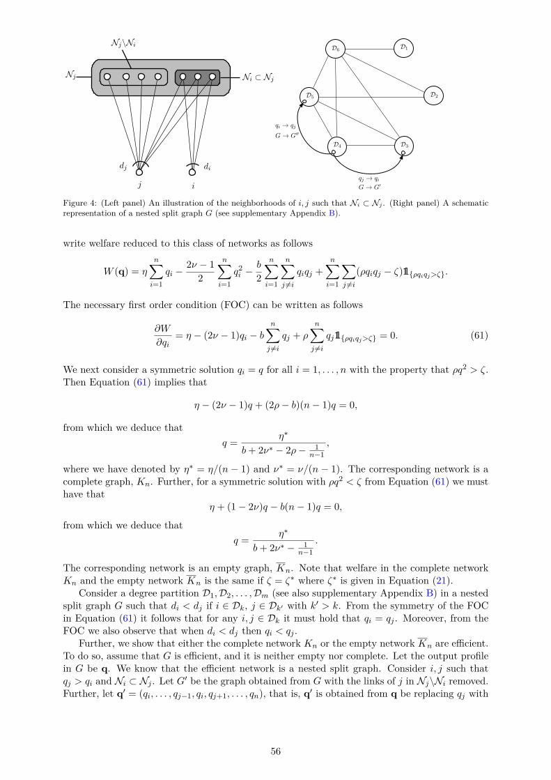
j i
Nj Ni ⊂ Nj
Nj\Ni
dj di
D1
D2
D3D4
D5
D6
qi → qj
G→ G′′
qj → qiG→ G′
Figure 4: (Left panel) An illustration of the neighborhoods of i, j such that Ni ⊂ Nj . (Right panel) A schematicrepresentation of a nested split graph G (see supplementary Appendix B).
write welfare reduced to this class of networks as follows
W (q) = ηn∑i=1
qi −2ν − 1
2
n∑i=1
q2i −b
2
n∑i=1
n∑j =i
qiqj +n∑i=1
∑j =i
(ρqiqj − ζ)1ρqiqj>ζ.
The necessary first order condition (FOC) can be written as follows
∂W
∂qi= η − (2ν − 1)qi − b
n∑j =i
qj + ρn∑j =i
qj1ρqiqj>ζ = 0. (61)
We next consider a symmetric solution qi = q for all i = 1, . . . , n with the property that ρq2 > ζ.Then Equation (61) implies that
η − (2ν − 1)q + (2ρ− b)(n− 1)q = 0,
from which we deduce thatq =
η∗
b+ 2ν∗ − 2ρ− 1n−1
,
where we have denoted by η∗ = η/(n − 1) and ν∗ = ν/(n − 1). The corresponding network is acomplete graph, Kn. Further, for a symmetric solution with ρq2 < ζ from Equation (61) we musthave that
η + (1− 2ν)q − b(n− 1)q = 0,
from which we deduce thatq =
η∗
b+ 2ν∗ − 1n−1
.
The corresponding network is an empty graph, Kn. Note that welfare in the complete networkKn and the empty network Kn is the same if ζ = ζ∗ where ζ∗ is given in Equation (21).
Consider a degree partition D1,D2, . . . ,Dm (see also supplementary Appendix B) in a nestedsplit graph G such that di < dj if i ∈ Dk, j ∈ Dk′ with k′ > k. From the symmetry of the FOCin Equation (61) it follows that for any i, j ∈ Dk it must hold that qi = qj . Moreover, from theFOC we also observe that when di < dj then qi < qj .
Further, we show that either the complete network Kn or the empty network Kn are efficient.To do so, assume that G is efficient, and it is neither empty nor complete. Let the output profilein G be q. We know that the efficient network is a nested split graph. Consider i, j such thatqj > qi and Ni ⊂ Nj . Let G′ be the graph obtained from G with the links of j in Nj\Ni removed.Further, let q′ = (qi, . . . , qj−1, qi, qj+1, . . . , qn), that is, q′ is obtained from q be replacing qj with
56
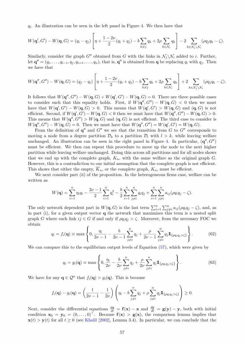
qi. An illustration can be seen in the left panel in Figure 4. We then have that
W (q′, G′)−W (q, G) = (qi − qj)
η + 1− 2ν
2(qi + qj)− b
∑k =j
qk + 2ρ∑k∈Ni
qk
− 2∑
k∈Nj\Ni
(ρqjqk − ζ).
Similarly, consider the graph G′′ obtained from G with the links in Nj\Ni added to i. Further,let q′′ = (qi, . . . , qi−1, qj , qi+1, . . . , qn), that is, q′′ is obtained from q be replacing qi with qj . Thenwe have that
W (q′′, G′′)−W (q, G) = (qj − qi)
η + 1− 2ν
2(qi + qj)− b
∑k =j
qk + 2ρ∑k∈Ni
qk
+ 2∑
k∈Nj\Ni
(ρqjqk − ζ).
It follows that W (q′′, G′′)−W (q, G) +W (q′, G′)−W (q, G) = 0. There are three possible casesto consider such that this equality holds. First, if W (q′′, G′′) − W (q, G) < 0 then we musthave that W (q′, G′) −W (q, G) > 0. This means that W (q′, G′) > W (q, G) and (q, G) is notefficient. Second, if W (q′, G′)−W (q, G) < 0 then we must have that W (q′′, G′′)−W (q, G) > 0.This means that W (q′′, G′′) > W (q, G) and (q, G) is not efficient. The third case to consider isW (q′′, G′′)−W (q, G) = 0. Then we must have that W (q′′, G′′) =W (q′, G′) =W (q, G).
From the definition of q′′ and G′′ we see that the transition from G to G′′ corresponds tomoving a node from a degree partition Dk to a partition Dl with l > k, while leaving welfareunchanged. An illustration can be seen in the right panel in Figure 4. In particular, (q′′, G′′)must be efficient. We then can repeat this procedure to move up the node to the next higherpartition while leaving welfare unchanged. Doing this across all partitions and for all nodes showsthat we end up with the complete graph, Kn, with the same welfare as the original graph G.However, this is a contradiction to our initial assumption that the complete graph is not efficient.This shows that either the empty, Kn, or the complete graph, Kn, must be efficient.
We next consider part (ii) of the proposition. In the heterogeneous firms case, welfare can bewritten as
W (q) =n∑i=1
ηiqi −2ν − 1
2
n∑i=1
q2i −b
2
n∑i=1
n∑j =i
qiqj +n∑i=1
n∑j =i
aij(ρqiqj − ζ).
The only network dependent part in W (q, G) is the last term∑n
i=1
∑nj =i aij(ρqiqj − ζ), and, as
in part (i), for a given output vector q the network that maximizes this term is a nested splitgraph G where each link ij ∈ G if and only if ρqiqj > ζ. Moreover, from the necessary FOC weobtain
qi = fi(q) ≡ max
0,ηi
2ν − 1− b
2ν − 1
n∑j =i
qj +ρ
2ν − 1
n∑j =i
qj1ρqiqj>ζ
. (62)
We can compare this to the equilibrium output levels of Equation (57), which were given by
qi = gi(q) ≡ max
0,ηi2ν
− b
2ν
n∑j =i
qj +ρ
2ν
n∑j =i
qj1ρqiqj>ζ
. (63)
We have for any q ∈ Qn that fi(q) > gi(q). This is because
fi(q)− gi(q) =
(1
2ν − 1− 1
2ν
)ηi − bn∑j =i
qj + ρn∑j =i
qj1ρqiqj>ζ
≥ 0.
Next, consider the differential equations dxdt = f(x) − x and dy
dt = g(y) − y, both with initialcondition x0 = y0 = (0, . . . , 0)⊤. Because f(x) > g(x), the comparison lemma implies thatx(t) > y(t) for all t ≥ 0 (see Khalil [2002], Lemma 3.4). In particular, we can conclude that the
57

fixed point f(q) = q must be higher than the fixed point g(q) = q. That is, in the stochasticallystable equilibrium output levels are too low compared to the social optimum. Moreover, becausea link is only present if ρqiqj > ζ there are fewer links in the stochastically stable network thanin the efficient network. 2
58
For Online PublicationSupplement to “Network Formation with Local Complements and Global
Substitutes: The Case of R&D Networks”
Chih-Sheng Hsieha, Michael D. Königb, Xiaodong Liuc
aDepartment of Economics, Chinese University of Hong Kong, CUHK Shatin, Hong Kong, China.bDepartment of Economics, University of Zurich, Schönberggasse 1, CH-8001 Zurich, Switzerland.
cDepartment of Economics, University of Colorado Boulder, Boulder, Colorado 80309–0256, United States.
B. Definitions and Characterizations
A network (graph) G is the pair (N , E) consisting of a set of nodes (vertices) N = 1, . . . , n anda set of edges (links) E ⊂ N ×N between them. A link (i, j) is incident with nodes i and j. Theneighborhood of a node i ∈ N is the set Ni = j ∈ N : (i, j) ∈ E. The degree di of a node i ∈ Ngives the number of links incident to node i. Clearly, di = |Ni|. Let N (2)
i =∪j∈Ni
Nj\ (Ni ∪ i)denote the second-order neighbors of node i. Similarly, the k-th order neighborhood of node iis defined recursively from N (0)
i = i, N (1)i = Ni and N (k)
i =∪j∈N (k−1)
i
Nj\(∪k−1
l=0 N (l)i
). A
walk in G of length k from i to j is a sequence ⟨i0, i1, . . . , ik⟩ of nodes such that i0 = i, ik = j,ip = ip+1, and ip and ip+1 are (directly) linked, that is ipip+1 ∈ E , for all 0 ≤ p ≤ k − 1. Nodes iand j are said to be indirectly linked in G if there exists a walk from i to j in G containing nodesother than i and j. A pair of nodes i and j is connected if they are either directly or indirectlylinked. A node i ∈ N is isolated in G if Ni = ∅. The network G is said to be empty (denoted byKn) when all its nodes are isolated.
A subgraph, G′, of G is the graph of subsets of the nodes, N (G′) ⊆ N (G), and links, E(G′) ⊆E(G). A graph G is connected, if there is a path connecting every pair of nodes. OtherwiseG is disconnected. The components of a graph G are the maximally connected subgraphs. Acomponent is said to be minimally connected if the removal of any link makes the componentdisconnected.
Given a graph G and a set S ⊆ N , we say that GS is the subgraph G induced S whenever theadjacency matrix of GS is AS . We write G−S to denote the network GN\S , that is G−S is thenetwork that results after eliminating all the nodes in S.
A dominating set for a graph G = (N , E) is a subset S ⊆ N such that every node not in Sis connected to at least one member of S by a link. An independent set is a set of nodes in agraph in which no two nodes are adjacent. For example the central node in a star K1,n−1 formsa dominating set while the peripheral nodes form an independent set.
Let G = (N , E) be a graph whose distinct positive degrees are d(1) < d(2) < . . . < d(k), andlet d0 = 0 (even if no agent with degree 0 exists in G). Further, define Di = v ∈ N : dv = d(i)for i = 0, . . . , k. Then the set-valued vector D = (D0,D1, . . . ,Dk) is called the degree partitionof G. A nested split graph is a graph with a nested neighborhood structure such that the set ofneighbors of each node is contained in the set of neighbors of each higher degree node [Cvetkovicand Rowlinson, 1990; Mahadev and Peled, 1995]. Let D = (D0,D1, . . . ,Dk) be the degree partitionof a nested split graph G = (N , E). Then the nodes N can be partitioned in independent sets Di,i = 1, . . . ,
⌊k2
⌋and a dominating set
∪ki=⌊ k
2⌋+1Di in the graph G′ = (N\D0, E). Moreover, the
1
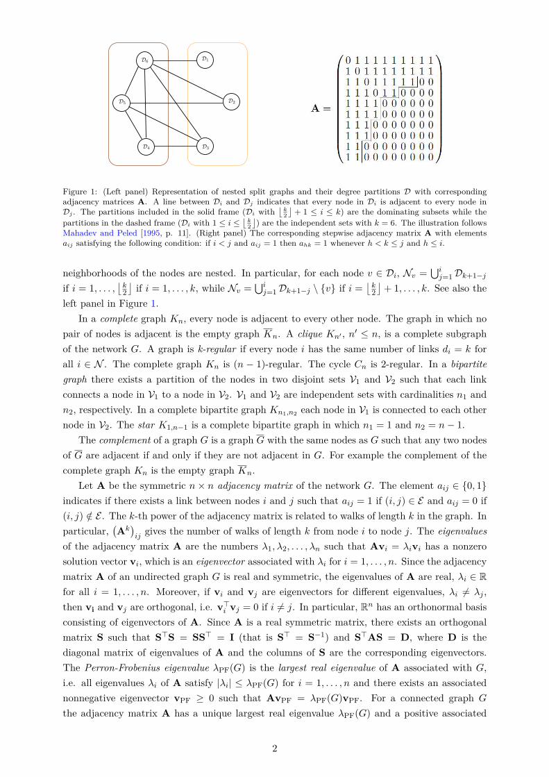
D1
D2
D3D4
D5
D6
Figure 1: (Left panel) Representation of nested split graphs and their degree partitions D with correspondingadjacency matrices A. A line between Di and Dj indicates that every node in Di is adjacent to every node inDj . The partitions included in the solid frame (Di with
⌊k2
⌋+ 1 ≤ i ≤ k) are the dominating subsets while the
partitions in the dashed frame (Di with 1 ≤ i ≤⌊k2
⌋) are the independent sets with k = 6. The illustration follows
Mahadev and Peled [1995, p. 11]. (Right panel) The corresponding stepwise adjacency matrix A with elementsaij satisfying the following condition: if i < j and aij = 1 then ahk = 1 whenever h < k ≤ j and h ≤ i.
neighborhoods of the nodes are nested. In particular, for each node v ∈ Di, Nv =∪ij=1Dk+1−j
if i = 1, . . . ,⌊k2
⌋if i = 1, . . . , k, while Nv =
∪ij=1Dk+1−j \ v if i =
⌊k2
⌋+ 1, . . . , k. See also the
left panel in Figure 1.In a complete graph Kn, every node is adjacent to every other node. The graph in which no
pair of nodes is adjacent is the empty graph Kn. A clique Kn′ , n′ ≤ n, is a complete subgraphof the network G. A graph is k-regular if every node i has the same number of links di = k forall i ∈ N . The complete graph Kn is (n − 1)-regular. The cycle Cn is 2-regular. In a bipartitegraph there exists a partition of the nodes in two disjoint sets V1 and V2 such that each linkconnects a node in V1 to a node in V2. V1 and V2 are independent sets with cardinalities n1 andn2, respectively. In a complete bipartite graph Kn1,n2 each node in V1 is connected to each othernode in V2. The star K1,n−1 is a complete bipartite graph in which n1 = 1 and n2 = n− 1.
The complement of a graph G is a graph G with the same nodes as G such that any two nodesof G are adjacent if and only if they are not adjacent in G. For example the complement of thecomplete graph Kn is the empty graph Kn.
Let A be the symmetric n× n adjacency matrix of the network G. The element aij ∈ 0, 1indicates if there exists a link between nodes i and j such that aij = 1 if (i, j) ∈ E and aij = 0 if(i, j) /∈ E . The k-th power of the adjacency matrix is related to walks of length k in the graph. Inparticular,
(Ak)ij
gives the number of walks of length k from node i to node j. The eigenvaluesof the adjacency matrix A are the numbers λ1, λ2, . . . , λn such that Avi = λivi has a nonzerosolution vector vi, which is an eigenvector associated with λi for i = 1, . . . , n. Since the adjacencymatrix A of an undirected graph G is real and symmetric, the eigenvalues of A are real, λi ∈ Rfor all i = 1, . . . , n. Moreover, if vi and vj are eigenvectors for different eigenvalues, λi = λj ,then vi and vj are orthogonal, i.e. v⊤
i vj = 0 if i = j. In particular, Rn has an orthonormal basisconsisting of eigenvectors of A. Since A is a real symmetric matrix, there exists an orthogonalmatrix S such that S⊤S = SS⊤ = I (that is S⊤ = S−1) and S⊤AS = D, where D is thediagonal matrix of eigenvalues of A and the columns of S are the corresponding eigenvectors.The Perron-Frobenius eigenvalue λPF(G) is the largest real eigenvalue of A associated with G,i.e. all eigenvalues λi of A satisfy |λi| ≤ λPF(G) for i = 1, . . . , n and there exists an associatednonnegative eigenvector vPF ≥ 0 such that AvPF = λPF(G)vPF. For a connected graph G
the adjacency matrix A has a unique largest real eigenvalue λPF(G) and a positive associated
2
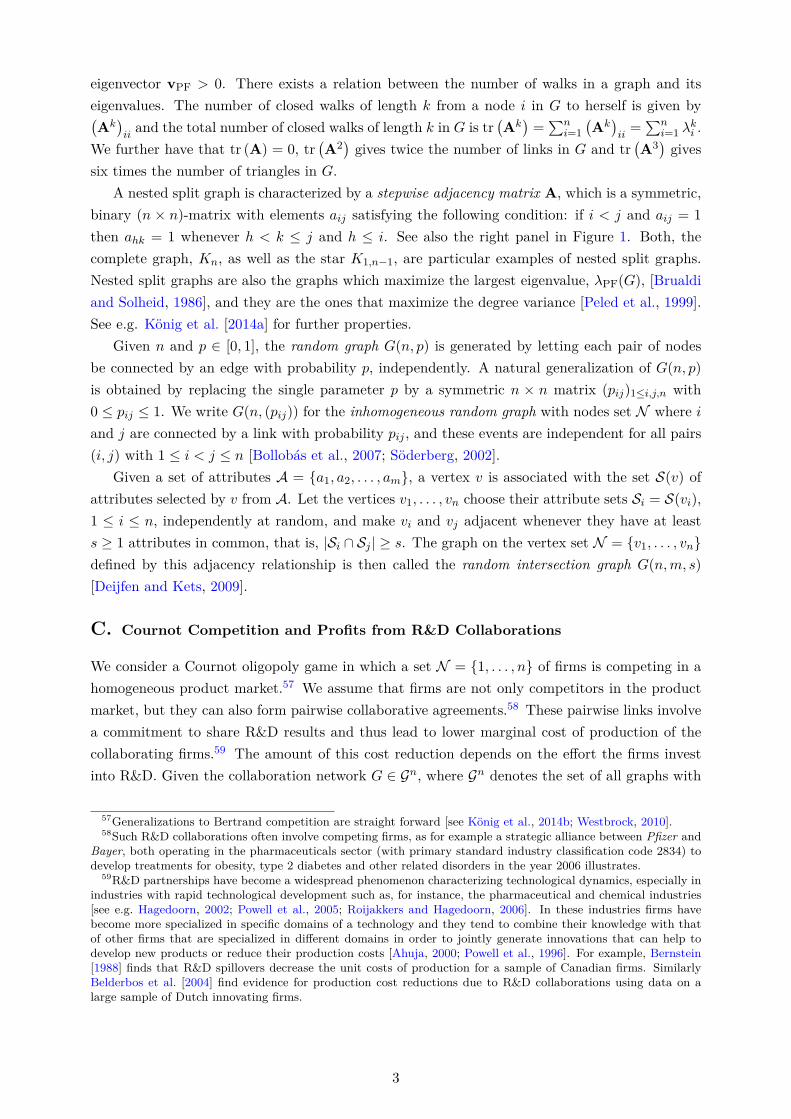
eigenvector vPF > 0. There exists a relation between the number of walks in a graph and itseigenvalues. The number of closed walks of length k from a node i in G to herself is given by(Ak)ii
and the total number of closed walks of length k in G is tr(Ak)=∑n
i=1
(Ak)ii=∑n
i=1 λki .
We further have that tr (A) = 0, tr(A2)
gives twice the number of links in G and tr(A3)
givessix times the number of triangles in G.
A nested split graph is characterized by a stepwise adjacency matrix A, which is a symmetric,binary (n × n)-matrix with elements aij satisfying the following condition: if i < j and aij = 1
then ahk = 1 whenever h < k ≤ j and h ≤ i. See also the right panel in Figure 1. Both, thecomplete graph, Kn, as well as the star K1,n−1, are particular examples of nested split graphs.Nested split graphs are also the graphs which maximize the largest eigenvalue, λPF(G), [Brualdiand Solheid, 1986], and they are the ones that maximize the degree variance [Peled et al., 1999].See e.g. König et al. [2014a] for further properties.
Given n and p ∈ [0, 1], the random graph G(n, p) is generated by letting each pair of nodesbe connected by an edge with probability p, independently. A natural generalization of G(n, p)is obtained by replacing the single parameter p by a symmetric n × n matrix (pij)1≤i,j,n with0 ≤ pij ≤ 1. We write G(n, (pij)) for the inhomogeneous random graph with nodes set N where iand j are connected by a link with probability pij , and these events are independent for all pairs(i, j) with 1 ≤ i < j ≤ n [Bollobás et al., 2007; Söderberg, 2002].
Given a set of attributes A = a1, a2, . . . , am, a vertex v is associated with the set S(v) ofattributes selected by v from A. Let the vertices v1, . . . , vn choose their attribute sets Si = S(vi),1 ≤ i ≤ n, independently at random, and make vi and vj adjacent whenever they have at leasts ≥ 1 attributes in common, that is, |Si ∩ Sj | ≥ s. The graph on the vertex set N = v1, . . . , vndefined by this adjacency relationship is then called the random intersection graph G(n,m, s)
[Deijfen and Kets, 2009].
C. Cournot Competition and Profits from R&D Collaborations
We consider a Cournot oligopoly game in which a set N = 1, . . . , n of firms is competing in ahomogeneous product market.57 We assume that firms are not only competitors in the productmarket, but they can also form pairwise collaborative agreements.58 These pairwise links involvea commitment to share R&D results and thus lead to lower marginal cost of production of thecollaborating firms.59 The amount of this cost reduction depends on the effort the firms investinto R&D. Given the collaboration network G ∈ Gn, where Gn denotes the set of all graphs with
57Generalizations to Bertrand competition are straight forward [see König et al., 2014b; Westbrock, 2010].58Such R&D collaborations often involve competing firms, as for example a strategic alliance between Pfizer and
Bayer, both operating in the pharmaceuticals sector (with primary standard industry classification code 2834) todevelop treatments for obesity, type 2 diabetes and other related disorders in the year 2006 illustrates.
59R&D partnerships have become a widespread phenomenon characterizing technological dynamics, especially inindustries with rapid technological development such as, for instance, the pharmaceutical and chemical industries[see e.g. Hagedoorn, 2002; Powell et al., 2005; Roijakkers and Hagedoorn, 2006]. In these industries firms havebecome more specialized in specific domains of a technology and they tend to combine their knowledge with thatof other firms that are specialized in different domains in order to jointly generate innovations that can help todevelop new products or reduce their production costs [Ahuja, 2000; Powell et al., 1996]. For example, Bernstein[1988] finds that R&D spillovers decrease the unit costs of production for a sample of Canadian firms. SimilarlyBelderbos et al. [2004] find evidence for production cost reductions due to R&D collaborations using data on alarge sample of Dutch innovating firms.
3
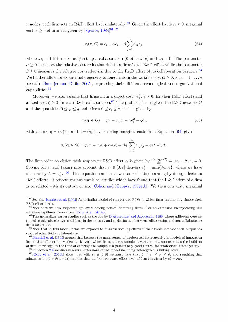
n nodes, each firm sets an R&D effort level unilaterally.60 Given the effort levels ei ≥ 0, marginalcost ci ≥ 0 of firm i is given by [Spence, 1984]61,62
ci(e, G) = ci − αei − β
n∑j=1
aijej , (64)
where aij = 1 if firms i and j set up a collaboration (0 otherwise) and aii = 0. The parameterα ≥ 0 measures the relative cost reduction due to a firms’ own R&D effort while the parameterβ ≥ 0 measures the relative cost reduction due to the R&D effort of its collaboration partners.63
We further allow for ex ante heterogeneity among firms in the variable cost ci ≥ 0, for i = 1, . . . , n
[see also Banerjee and Duflo, 2005], expressing their different technological and organizationalcapabilities.64
Moreover, we also assume that firms incur a direct cost γe2i , γ ≥ 0, for their R&D efforts anda fixed cost ζ ≥ 0 for each R&D collaboration.65 The profit of firm i, given the R&D network Gand the quantities 0 ≤ qi ≤ q and efforts 0 ≤ ei ≤ e, is then given by
πi(q, e, G) = (pi − ci)qi − γe2i − ζdi, (65)
with vectors q = (qi)ni=1 and e = (ei)
ni=1. Inserting marginal costs from Equation (64) gives
πi(q, e, G) = piqi − ciqi + αqiei + βqi
n∑j=1
aijej − γe2i − ζdi.
The first-order condition with respect to R&D effort ei is given by ∂πi(q,e,G)∂ei
= αqi − 2γei = 0.Solving for ei and taking into account that ei ∈ [0, e] delivers e∗i = minλqi, e, where we havedenoted by λ = α
2γ . 66 This equation can be viewed as reflecting learning-by-doing effects onR&D efforts. It reflects various empirical studies which have found that the R&D effort of a firmis correlated with its output or size [Cohen and Klepper, 1996a,b]. We then can write marginal
60See also Kamien et al. [1992] for a similar model of competitive RJVs in which firms unilaterally choose theirR&D effort levels.
61Note that we have neglected spillovers among non-collaborating firms. For an extension incorporating thisadditional spillover channel see König et al. [2014b].
62This generalizes earlier studies such as the one by D’Aspremont and Jacquemin [1988] where spillovers were as-sumed to take place between all firms in the industry and no distinction between collaborating and non-collaboratingfirms was made.
63Note that in this model, firms are exposed to business stealing effects if their rivals increase their output viacost reducing R&D collaborations.
64Blundell et al. [1995] argued that because the main source of unobserved heterogeneity in models of innovationlies in the different knowledge stocks with which firms enter a sample, a variable that approximates the build-upof firm knowledge at the time of entering the sample is a particularly good control for unobserved heterogeneity.
65In Section 2.4 we discuss several extensions of the model including heterogeneous linking costs.66König et al. [2014b] show that with qi ∈ [0, q] we must have that 0 ≤ ei ≤ qi ≤ q, and requiring that
mini∈N ci > q(1 + β(n− 1)), implies that the best response effort level of firm i is given by e∗i = λqi.
4
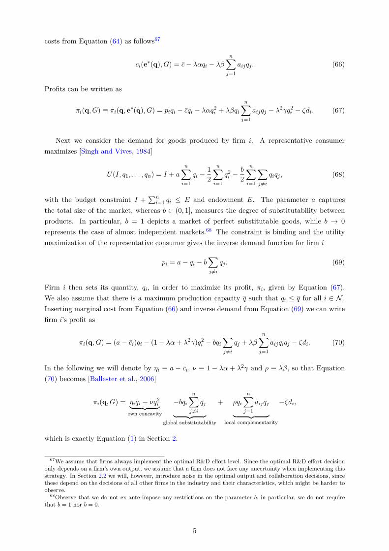
costs from Equation (64) as follows67
ci(e∗(q), G) = c− λαqi − λβ
n∑j=1
aijqj . (66)
Profits can be written as
πi(q, G) ≡ πi(q, e∗(q), G) = piqi − cqi − λαq2i + λβqi
n∑j=1
aijqj − λ2γq2i − ζdi. (67)
Next we consider the demand for goods produced by firm i. A representative consumermaximizes [Singh and Vives, 1984]
U(I, q1, . . . , qn) = I + a
n∑i=1
qi −1
2
n∑i=1
q2i −b
2
n∑i=1
∑j =i
qiqj , (68)
with the budget constraint I +∑n
i=1 qi ≤ E and endowment E. The parameter a capturesthe total size of the market, whereas b ∈ (0, 1], measures the degree of substitutability betweenproducts. In particular, b = 1 depicts a market of perfect substitutable goods, while b → 0
represents the case of almost independent markets.68 The constraint is binding and the utilitymaximization of the representative consumer gives the inverse demand function for firm i
pi = a− qi − b∑j =i
qj . (69)
Firm i then sets its quantity, qi, in order to maximize its profit, πi, given by Equation (67).We also assume that there is a maximum production capacity q such that qi ≤ q for all i ∈ N .Inserting marginal cost from Equation (66) and inverse demand from Equation (69) we can writefirm i’s profit as
πi(q, G) = (a− ci)qi − (1− λα+ λ2γ)q2i − bqi∑j =i
qj + λβn∑j=1
aijqiqj − ζdi. (70)
In the following we will denote by ηi ≡ a − ci, ν ≡ 1 − λα + λ2γ and ρ ≡ λβ, so that Equation(70) becomes [Ballester et al., 2006]
πi(q, G) = ηiqi − νq2i︸ ︷︷ ︸own concavity
−bqin∑j =i
qj︸ ︷︷ ︸global substitutability
+ ρqi
n∑j=1
aijqj︸ ︷︷ ︸local complementarity
−ζdi,
which is exactly Equation (1) in Section 2.
67We assume that firms always implement the optimal R&D effort level. Since the optimal R&D effort decisiononly depends on a firm’s own output, we assume that a firm does not face any uncertainty when implementing thisstrategy. In Section 2.2 we will, however, introduce noise in the optimal output and collaboration decisions, sincethese depend on the decisions of all other firms in the industry and their characteristics, which might be harder toobserve.
68Observe that we do not ex ante impose any restrictions on the parameter b, in particular, we do not requirethat b = 1 nor b = 0.
5
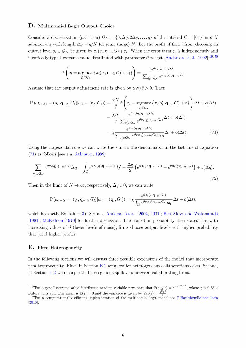
D. Multinomial Logit Output Choice
Consider a discretization (partition) QN = 0,∆q, 2∆q, . . . , q of the interval Q = [0, q] into Nsubintervals with length ∆q = q/N for some (large) N . Let the profit of firm i from choosing anoutput level qi ∈ QN be given by πi(qi,q−i, G)+ εi. When the error term εi is independently andidentically type-I extreme value distributed with parameter ϑ we get [Anderson et al., 1992]:69,70
P
(qi = argmax
q′i∈Qs
πi(qi,q−i, G) + εi
)=
eϑπi(qi,q−i,G)∑q′i∈QN
eϑπi(q′i,q−i,G)
.
Assume that the output adjustment rate is given by χN/q > 0. Then
P (ωt+∆t = (qi,q−it, Gt)|ωt = (qt, Gt)) =χN
qP
(qi = argmax
q′i∈Qs
πi(q
′i,q−i, G) + ε
)∆t+ o(∆t)
=χN
q
eϑπi(qi,q−it,Gt)∑q′i∈QN
eϑπi(q′i,q−it,Gt)
∆t+ o(∆t)
= χeϑπi(qi,q−it,Gt)∑
q′i∈QNeϑπi(q
′i,q−it,Gt)∆q
∆t+ o(∆t). (71)
Using the trapezoidal rule we can write the sum in the denominator in the last line of Equation(71) as follows [see e.g. Atkinson, 1989]
∑q′i∈QN
eϑπi(q′i,q−it,Gt)∆q =
∫Qeϑπi(q
′,q−it,Gt)dq′ +∆q
2
(eϑπi(0,q−it,Gt) + eϑπi(q,q−it,Gt)
)+ o(∆q).
(72)Then in the limit of N → ∞, respectively, ∆q ↓ 0, we can write
P (ωt+∆t = (qi,q−it, Gt)|ωt = (qt, Gt)) = χeϑπi(q,q−it,Gt)∫
Q eϑπi(q′,q−it,Gt)dq′
∆t+ o(∆t),
which is exactly Equation (3). See also Anderson et al. [2004, 2001]; Ben-Akiva and Watanatada[1981]; McFadden [1976] for further discussion. The transition probability then states that withincreasing values of ϑ (lower levels of noise), firms choose output levels with higher probabilitythat yield higher profits.
E. Firm Heterogeneity
In the following sections we will discuss three possible extensions of the model that incorporatefirm heterogeneity. First, in Section E.1 we allow for heterogeneous collaborations costs. Second,in Section E.2 we incorporate heterogenous spillovers between collaborating firms.
69For a type-I extreme value distributed random variable ε we have that P(ε ≤ c) = e−ec/ζ−γ , where γ ≈ 0.58 isEuler’s constant. The mean is E(ε) = 0 and the variance is given by Var(ε) = π2ζ2
6.
70For a computationally efficient implementation of the multinomial logit model see D’Haultfœuille and Iaria[2016].
6
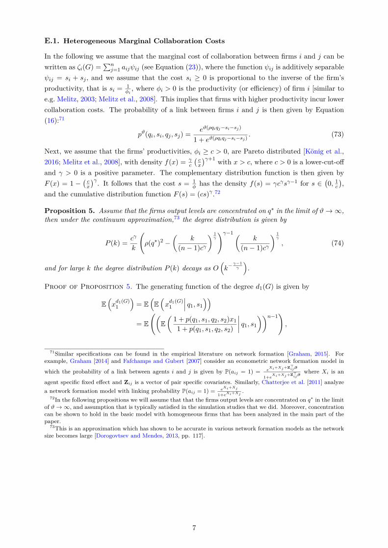
E.1. Heterogeneous Marginal Collaboration Costs
In the following we assume that the marginal cost of collaboration between firms i and j can bewritten as ζi(G) =
∑nj=1 aijψij (see Equation (23)), where the function ψij is additively separable
ψij = si + sj , and we assume that the cost si ≥ 0 is proportional to the inverse of the firm’sproductivity, that is si = 1
ϕi, where ϕi > 0 is the productivity (or efficiency) of firm i [similar to
e.g. Melitz, 2003; Melitz et al., 2008]. This implies that firms with higher productivity incur lowercollaboration costs. The probability of a link between firms i and j is then given by Equation(16):71
pϑ(qi, si, qj , sj) =eϑ(ρqiqj−si−sj)
1 + eϑ(ρqiqj−si−sj). (73)
Next, we assume that the firms’ productivities, ϕi ≥ c > 0, are Pareto distributed [König et al.,2016; Melitz et al., 2008], with density f(x) = γ
c
(cx
)γ+1 with x > c, where c > 0 is a lower-cut-offand γ > 0 is a positive parameter. The complementary distribution function is then given byF (x) = 1 −
(cx
)γ . It follows that the cost s = 1ϕ has the density f(s) = γcγsγ−1 for s ∈
(0, 1c),
and the cumulative distribution function F (s) = (cs)γ .72
Proposition 5. Assume that the firms output levels are concentrated on q∗ in the limit of ϑ→ ∞,then under the continuum approximation,73 the degree distribution is given by
P (k) =cγ
k
(ρ(q∗)2 −
(k
(n− 1)cγ
) 1γ
)γ−1(k
(n− 1)cγ
) 1γ
, (74)
and for large k the degree distribution P (k) decays as O(k− γ−1
γ
).
Proof of Proposition 5. The generating function of the degree d1(G) is given by
E(xd1(G)1
)= E
(E(xd1(G)1
∣∣∣ q1, s1))= E
((E(1 + p(q1, s1, q2, s2)x11 + p(q1, s1, q2, s2)
∣∣∣∣ q1, s1))n−1),
71Similar specifications can be found in the empirical literature on network formation [Graham, 2015]. Forexample, Graham [2014] and Fafchamps and Gubert [2007] consider an econometric network formation model in
which the probability of a link between agents i and j is given by P(aij = 1) = eXi+Xj+Z⊤
ijβ
1+eXi+Xj+Z⊤
ijβ
where Xi is an
agent specific fixed effect and Zij is a vector of pair specific covariates. Similarly, Chatterjee et al. [2011] analyzea network formation model with linking probability P(aij = 1) = e
Xi+Xj
1+eXi+Xj
.72In the following propositions we will assume that that the firms output levels are concentrated on q∗ in the limit
of ϑ→ ∞, and assumption that is typically satisfied in the simulation studies that we did. Moreover, concentrationcan be shown to hold in the basic model with homogeneous firms that has been analyzed in the main part of thepaper.
73This is an approximation which has shown to be accurate in various network formation models as the networksize becomes large [Dorogovtsev and Mendes, 2013, pp. 117].
7

With the cost distributed as f(s) = γcγsγ−1 for s ∈(0, 1c), we can write
E(xd1(G)1
∣∣∣ q1 = q, s1 = s)= E
(1 + p(q, s, q2, s2)x11 + p(q, s, q2, s2)
∣∣∣∣ q, s)n−1
= (1 + (x1 − 1)E (p(q, s, q2, s2)| q1 = q, s1 = s))n−1
=
(1 + (x1 − 1)
∫Qdq′µϑ(q′)
∫ds′γcγ(s′)γ−1p(q, s, q′, s′)
)n−1
=
(1 + (x1 − 1)
∫Qdq′µϑ(q′)
∫ds′γcγ(s′)γ−1 eϑ(ρqq
′−s−s′)
1 + eϑ(ρqq′−s−s′)
)n−1
.
In the limit of ϑ→ ∞ in Equation (73) we obtain
limϑ→∞
pϑ(q, s, q′, s′) = limϑ→∞
eϑ(ρqq′−s−s′)
1 + eϑ(ρqq′−s−s′)= 1ρqq′>s+s′,
so that we can write
E(xd1(G)1
∣∣∣ q1 = q, s1 = s)=
(1 + (x1 − 1)
∫Qdq′µϑ(q′)
∫ds′γcγ(s′)γ−11ρqq′>s+s′
)n−1
=
(1 + (x1 − 1)γcγ
∫ ρqq∗−s
0ds′(s′)γ−1
)n−1
= (1 + (x1 − 1)cγ (ρqq∗ − s)γ)n−1
= e(x1−1)(n−1)cγ(ρqq∗−s)γ .
This is the generating function of a Poisson random variable with expectation and variance givenby d(q, s) ≡ (n−1)cγ (ρqq∗ − s)γ . When the cut-off c is small, the variance becomes small, and wecan approximate the Poisson random variable with a constant random variable at the expectedvalue. Making further a continuum approximation, where we treat the degree as a continuousvariable, we can write
P (d1(G) = k| q1 = q, s1 = s) = δ(k − d(q, s)
)= δ (k − (n− 1)cγ (ρqq∗ − s)γ) .
Note that under the continuum approximation there exists a one-to-one mapping from the degreek to the cost s, where for a given k and output q, the cost s is given by
s = ρqq∗ −(
k
(n− 1)cγ
) 1γ
.
Using the fact that74
δ(k − (n− 1)cγ
(ρ(q∗)2 − s
)γ)= δ
(s−
(ρ(q∗)2 −
(k
(n− 1)cγ
) 1γ
))1
γk
(k
(n− 1)cγ
) 1γ
. (75)
74When g(x) is a continuously differentiable function in R it holds that δ(g(x)) =∑m
i=1δ(x−xi)|g′(xi)|
where the mroots xi satisfy g(xi) = 0 for all i = 1, . . . ,m.
8
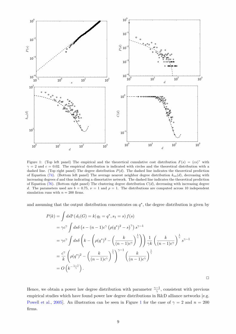
10−1
100
101
102
10−6
10−4
10−2
100
s
P(s)
100
101
102
103
10−4
10−3
10−2
10−1
100
d
P(d)
100
101
102
103
101
102
d
knn(d)
100
101
102
103
10−1
100
d
C(d)
Figure 1: (Top left panel) The empirical and the theoretical cumulative cost distribution F (s) = (cs)γ withγ = 2 and c = 0.02. The empirical distribution is indicated with circles and the theoretical distribution with adashed line. (Top right panel) The degree distribution P (d). The dashed line indicates the theoretical predictionof Equation (74). (Bottom left panel) The average nearest neighbor degree distribution knn(d), decreasing withincreasing degrees d and thus indicating a dissortative network. The dashed line indicates the theoretical predictionof Equation (76). (Bottom right panel) The clustering degree distribution C(d), decreasing with increasing degreed. The parameters used are b = 0.75, ν = 1 and ρ = 1. The distributions are computed across 10 independentsimulation runs with n = 200 firms.
and assuming that the output distribution concentrates on q∗, the degree distribution is given by
P (k) =
∫dsP (d1(G) = k| q1 = q∗, s1 = s) f(s)
= γcγ∫dsδ
(s− (n− 1)cγ
(ρ(q∗)2 − s
)γ)sγ−1
= γcγ∫dsδ
(k −
(ρ(q∗)2 −
(k
(n− 1)cγ
) 1γ
))1
γk
(k
(n− 1)cγ
) 1γ
sγ−1
=cγ
k
(ρ(q∗)2 −
(k
(n− 1)cγ
) 1γ
)γ−1(k
(n− 1)cγ
) 1γ
= O(k− γ−1
γ
).
2
Hence, we obtain a power law degree distribution with parameter γ−1γ , consistent with previous
empirical studies which have found power law degree distributions in R&D alliance networks [e.g.Powell et al., 2005]. An illustration can be seen in Figure 1 for the case of γ = 2 and n = 200
firms.
9
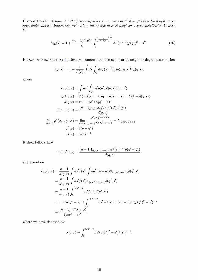
Proposition 6. Assume that the firms output levels are concentrated on q∗ in the limit of ϑ→ ∞,then under the continuum approximation, the averge nearest neighbor degree distribution is givenby
knn(k) = 1 +(n− 1)2γc2γ
k
∫ (k
(n−1)cγ
) 1γ
0ds′(s′γ−1(ρ(q∗)2 − s′γ . (76)
Proof of Proposition 6. Next we compute the average nearest neighbor degree distribution
knn(k) = 1 +1
P (k)
∫ds
∫Qdqf(s)µϑ(q)g(k|q, s)knn(q, s),
where
knn(q, s) =
∫ds′∫Qdq′p(q′, s′|q, s)d(q′, s′),
g(k|q, s) = P (d1(G) = k| q1 = q, s1 = s) = δ(k − d(q, s)
),
d(q, s) = (n− 1)cγ (ρqq∗ − s)γ
p(q′, s′|q, s) = (n− 1)p(q, s, q′, s′)f(s′)µϑ(q′)
d(q, s),
limϑ→∞
pϑ(q, s, q′, s′) = limϑ→∞
eϑ(ρqq′−s−s′)
1 + eϑ(ρqq′−s−s′)= 1ρqq′>s+s′
µϑ(q) = δ(q − q∗)
f(s) = γcγsγ−1.
It then follows that
p(q′, s′|q, s) =(n− 1)1ρqq′>s+s′γc
γ(s′)γ−1δ(q′ − q∗)
d(q, s),
and therefore
knn(q, s) =n− 1
d(q, s)
∫ds′f(s′)
∫dq′δ(q − q∗)1ρqq′>s+s′d(q
′, s′)
=n− 1
d(q, s)
∫ds′f(s′)1ρqq∗>s+s′d(q
∗, s′)
=n− 1
d(q, s)
∫ ρqq∗−s
0ds′f(s′)d(q∗, s′)
= c−γ(ρqq∗ − s)−γ∫ ρqq∗−s
0ds′γcγ(s′)γ−1(n− 1)cγ(ρ(q∗)2 − s′)−γ
=(n− 1)γcγJ(q, s)
(ρqq∗ − s)γ,
where we have denoted by
J(q, s) ≡∫ ρqq∗−s
0ds′(ρ(q∗)2 − s′)γ(s′)γ−1.
10

We then get
knn(k) = 1 +1
P (k)
∫ds
∫Qdqf(s)δ(q − q∗)δ
(k − d(q, s)
)knn(q, s)
= 1 +1
P (k)
∫dsγcγsγ−1δ
(k − d(q∗, s)
)knn(q
∗, s)
= 1 +1
P (k)
∫dsf(s)δ
(k − d(q∗, s)
) (n− 1)γcγJ(q∗, s)
(ρqq∗ − s)γ.
Using Equation (75) we can write this as
knn(k) = 1 +1
P (k)γcγ
(ρ(q∗)2 −
(k
(n− 1)cγ
) 1γ
)γ−11
γk
(k
(n− 1)cγ
) 1γ
× (n− 1)cγγJ
(q∗, ρ(q∗)2 −
(k
(n− 1)cγ
) 1γ
)
= 1 +(n− 1)2γc2γ
kJ
(q∗, ρ(q∗)2 −
(k
(n− 1)cγ
) 1γ
)
= 1 +(n− 1)2γc2γ
k
∫ (k
(n−1)cγ
) 1γ
0ds′(s′)γ−1(ρ(q∗)2 − s′)γ .
2
Figure 1 shows the results from numerical simulations compared with the theoretical predictionof Equation (76).
Proposition 7. Assume that the firms output levels are concentrated on q∗ in the limit of ϑ→ ∞,then under the continuum approximation, the clustering coefficient is given by
C(k) = 1k<(n−1)
(ρ(q∗)2c
2
)γ + 1k>(n−1)
(ρ(q∗)2c
2
)γ (n− 1)cγ
k
×
1 + γ(n− 1)cγ
k
∫ (k
(n−1)cγ
) 1γ
ρ(q∗)2−(
k(n−1)cγ
) 1γds′(s′γ−1
(ρ(q∗)2 − s′
)γ , (77)
and for large k the clustering coefficient C(k) decays as O(1k
).
Proof of Proposition 7. Next we analyze the clustering coefficient of a firm with degree k,which can be written as
C(k) =1
P (k)
∫ds
∫Qdqf(s)δ(q − q∗)g(k|q, s)C(q, s)
=1
P (k)
∫dsf(s)g(k|q∗, s)C(q∗, s),
where
C(q∗, s) =
∫ds′∫ds′′
∫Qdq′∫Qdq′′p(q′, s′, q′′, s′′)p(q′, s′|q∗, s)p(q′′, s′′|q∗, s).
11

This can further be written as follows
C(q∗, s) =
∫ds′∫ds′′
∫Qdq′∫Qdq′′1ρq′q′′>s′+s′′
×(n− 1)1ρq∗q′>s+s′f(s
′)δ(q′ − q∗)
d(q∗, s)
(n− 1)1ρq∗q′′>s+s′′f(s′′)δ(q′′ − q∗)
d(q∗, s)
=(n− 1)2
d(q∗, s)2
∫ds′f(s′)
∫ds′′f(s′′)1ρ(q∗)2>s′+s′′1ρ(q∗)2>s+s′1ρ(q∗)2>s+s′′
=(n− 1)2
d(q∗, s)2
(1
s>ρ(q∗)2
2
∫ ρ(q∗)2−s
0ds′f(s′)
∫ ρ(q∗)2−s
0ds′′f(s′′)
+1s<
ρ(q∗)22
(∫ s
0ds′f(s′)
∫ ρ(q∗)2−s
0ds′′f(s′′) +
∫ ρ(q∗)2−s
sds′f(s′)
∫ ρ(q∗)2−s′
0ds′′f(s′′)
)).
We then get (see also Figure 2)
C(q∗, s) =γ2c2γ(n− 1)2
d(q∗, s)
(1
s<ρ(q∗)2
2
∫ ρ(q∗)2−s
0ds′(s′)γ−1
∫ ρ(q∗)2−s
0ds′′(s′′)γ−1
+1s>
ρ(q∗)22
(∫ s
0ds′(s′)γ−1
∫ ρ(q∗)2−s
0ds′′(s′′)γ−1 +
∫ ρ(q∗)2−s
sds′(s′)γ−1
∫ ρ(q∗)2−s′
0ds′′(s′′)γ−1
))
=γc2γ(n− 1)2
d(q∗, s)
(1
s<ρ(q∗)2
2
∫ ρ(q∗)2−s
0ds′(s′)γ−1
(ρ(q∗)2 − s
)γ+1
s>ρ(q∗)2
2
(∫ s
0ds′(s′)γ−1
(ρ(q∗)2 − s
)γ+
∫ ρ(q∗)2−s
sds′(s′)γ−1
(ρ(q∗)2 − s′
)γ))
=γc2γ(n− 1)2
d(q∗, s)
(1
s<ρ(q∗)2
2
1γ
(ρ(q∗)2 − s
)2γ+1
s>ρ(q∗)2
2
(1
γsγ(ρ(q∗)2 − s
)γ+
∫ ρ(q∗)2−s
sds′(s′)γ−1
(ρ(q∗)2 − s′
)γ))
=c2γ(n− 1)2
d(q∗, s)
(1
s<ρ(q∗)2
2
(ρ(q∗)2 − s)2γ
+ 1s>
ρ(q∗)22
(sγ (ρ(q∗)2 − s)γ
+ γJ(s)))
,
(78)
where we have denoted by
J(s) ≡∫ ρ(q∗)2−s
sds′(s′)γ−1
(ρ(q∗)2 − s′
)γ.
Using the fact that d(q, s) ≡ (n− 1)cγ (ρqq∗ − s)γ this can be written as
C(q∗, s) =1
(ρ(q∗)2 − s)2γ
(1
s<ρ(q∗)2
2
(ρ(q∗)2 − s)2γ
+ 1s>
ρ(q∗)22
(sγ (ρ(q∗)2 − s)γ
+ γJ(s)))
.
(79)
12

s′
s′′
sρ(q∗)2 − s
ρ(q∗)2 − s
ρ(q∗)2 = s′ + s′′
1/c
1/c
s′
s′′
s ρ(q∗)2 − s
ρ(q∗)2 − s
ρ(q∗)2 = s′ + s′′
1/c
1/c
Figure 2: The area of integration in Equation (78) for the case of s < ρ(q∗)2
2(left panel) and for the case of
s > ρ(q∗)2
2(right panel).
Hence we get
C(k) =1
P (k)
∫dsf(s)δ
(k − d(q∗, s)
)C(q∗, s)
=1
P (k)
∫dsγcγsγ−1δ
(s−
(ρ(q∗)2 −
(k
(n− 1)cγ
) 1γ
))1
γk
(k
(n− 1)cγ
) 1γ
C(q∗, s)
=1
P (k)γcγ
(ρ(q∗)2 −
(k
(n− 1)cγ
) 1γ
)γ−11
γk
(k
(n− 1)cγ
) 1γ
C
(q∗, ρ(q∗)2 −
(k
(n− 1)cγ
) 1γ
)
= C
(q∗, ρ(q∗)2 −
(k
(n− 1)cγ
) 1γ
).
Inserting Equation (79) this gives
C(k) = 1k<(n−1)
(ρ(q∗)2c
2
)γ + 1k>(n−1)
(ρ(q∗)2c
2
)γ((n− 1)cγ
k+ γ
((n− 1)cγ
k
)2
J
(ρ(q∗)2 −
(k
(n− 1)cγ
) 1γ
))
= 1k<(n−1)
(ρ(q∗)2c
2
)γ + 1k>(n−1)
(ρ(q∗)2c
2
)γ((n− 1)cγ
k
+ γ
((n− 1)cγ
k
)2 ∫ (k
(n−1)cγ
) 1γ
ρ(q∗)2−(
k(n−1)cγ
) 1γds′(s′)γ−1
(ρ(q∗)2 − s′
)γ2
Figure 1 shows the results from numerical simulations compared with the theoretical prediction ofEquation (77). The figure further illustrates that the model can generate two-vertex and three-vertex degree correlations, such as a decreasing average nearest neighbor connectivity, knn(d),indicating a dissortative network, as well as a decreasing clustering degree distribution, C(d),with the degree d.
E.2. Heterogeneous Technology Spillovers
In this section we allow for heterogeneity among firms in terms of their technological abilities
13
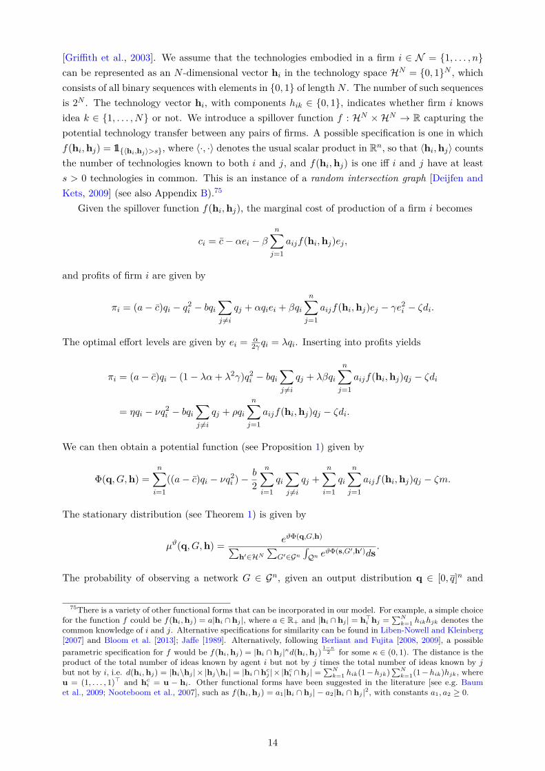
[Griffith et al., 2003]. We assume that the technologies embodied in a firm i ∈ N = 1, . . . , ncan be represented as an N -dimensional vector hi in the technology space HN = 0, 1N , whichconsists of all binary sequences with elements in 0, 1 of length N . The number of such sequencesis 2N . The technology vector hi, with components hik ∈ 0, 1, indicates whether firm i knowsidea k ∈ 1, . . . , N or not. We introduce a spillover function f : HN ×HN → R capturing thepotential technology transfer between any pairs of firms. A possible specification is one in whichf(hi,hj) = 1⟨hi,hj⟩>s, where ⟨·, ·⟩ denotes the usual scalar product in Rn, so that ⟨hi,hj⟩ countsthe number of technologies known to both i and j, and f(hi,hj) is one iff i and j have at leasts > 0 technologies in common. This is an instance of a random intersection graph [Deijfen andKets, 2009] (see also Appendix B).75
Given the spillover function f(hi,hj), the marginal cost of production of a firm i becomes
ci = c− αei − β
n∑j=1
aijf(hi,hj)ej ,
and profits of firm i are given by
πi = (a− c)qi − q2i − bqi∑j =i
qj + αqiei + βqi
n∑j=1
aijf(hi,hj)ej − γe2i − ζdi.
The optimal effort levels are given by ei = α2γ qi = λqi. Inserting into profits yields
πi = (a− c)qi − (1− λα+ λ2γ)q2i − bqi∑j =i
qj + λβqi
n∑j=1
aijf(hi,hj)qj − ζdi
= ηqi − νq2i − bqi∑j =i
qj + ρqi
n∑j=1
aijf(hi,hj)qj − ζdi.
We can then obtain a potential function (see Proposition 1) given by
Φ(q, G,h) =n∑i=1
((a− c)qi − νq2i )−b
2
n∑i=1
qi∑j =i
qj +n∑i=1
qi
n∑j=1
aijf(hi,hj)qj − ζm.
The stationary distribution (see Theorem 1) is given by
µϑ(q, G,h) =eϑΦ(q,G,h)∑
h′∈HN
∑G′∈Gn
∫Qn eϑΦ(s,G′,h′)ds
.
The probability of observing a network G ∈ Gn, given an output distribution q ∈ [0, q]n and
75There is a variety of other functional forms that can be incorporated in our model. For example, a simple choicefor the function f could be f(hi,hj) = a|hi ∩ hj |, where a ∈ R+ and |hi ∩ hj | = h⊤
i hj =∑N
k=1 hikhjk denotes thecommon knowledge of i and j. Alternative specifications for similarity can be found in Liben-Nowell and Kleinberg[2007] and Bloom et al. [2013]; Jaffe [1989]. Alternatively, following Berliant and Fujita [2008, 2009], a possibleparametric specification for f would be f(hi,hj) = |hi ∩ hj |κd(hi,hj)
1−κ2 for some κ ∈ (0, 1). The distance is the
product of the total number of ideas known by agent i but not by j times the total number of ideas known by jbut not by i, i.e. d(hi,hj) = |hi\hj |× |hj\hi| = |hi ∩hc
j |× |hci ∩hj | =
∑Nk=1 hik(1−hjk)
∑Nk=1(1−hik)hjk, where
u = (1, . . . , 1)⊤ and hci = u − hi. Other functional forms have been suggested in the literature [see e.g. Baum
et al., 2009; Nooteboom et al., 2007], such as f(hi,hj) = a1|hi ∩ hj | − a2|hi ∩ hj |2, with constants a1, a2 ≥ 0.
14

technology portfolios h ∈ HN is determined by the conditional distribution
µϑ(G|q,h) =∏i<j
eϑaij(ρf(hi,hj)qiqj−ζ)
1 + eϑ(ρf(hi,hj)qiqj−ζ), (80)
which is equivalent to the probability of observing an inhomogeneous random graph with linkprobability
pϑ(qi,hi, qj ,hj) ≡eϑ(ρf(hi,hj)qiqj−ζ)
1 + eϑ(ρf(hi,hj)qiqj−ζ). (81)
In the following we consider a particularly simple specification in which each firm i is assigneda technology k ∈ 1, . . . , N uniformly at random so that hik = 1 and hil = 0 for all l = k.Moreover, let f(hi,hj) = 1⟨hi,hj⟩≥1, that is, firms i an j can only benefit from a collaborationif they have a technology in common.
Proposition 8. Assume that each firm i is assigned a technology k ∈ 1, . . . , N uniformly atrandom and let f(hi,hj) = 1⟨hi,hj⟩≥1.
(i) The degree distribution is given by
P (k) =
(n
k
)(1
N
)k (1− 1
N
)n−k.
(ii) The average nearest neighbor degree distribution is given by
knn(k) =k(1− 1
N )(1 + n 1N − (n+ 1)
(1N
)n)
1N (1 + n− k)
, (82)
and for large n the average nearest neighbor degree distribution, knn(k), grows linearly asO(k).
(iii) The clustering coefficient is given by C(k) = 1.
Proof of Proposition 8. We first prove part (i) of the proposition. If technologies are as-signed uniformly at random then
P(⟨hi,hj⟩ ≥ 1| qi = q, qj = q′
)=
1
N1ρqq′>ζ.
Due to symmetry the firms quantities in the stationary state when ϑ→ ∞ are identical and givenby q∗. In the case of ρ(q∗)2 > ζ > 0 we then we have that
P (aij = 1) =1
N,
and the degree distribution is given by
P (k) = P (d1(G) = k) =
(n
k
)(1
N
)k (1− 1
N
)n−k.
We next give a proof of part (ii) of the proposition. The average nearest neighbor degreedistribution is then given by
knn(k) =n∑
k′=1
k′P(d2(G) = k′ − 1
∣∣ a12 = 1, d1(G) = k)
15
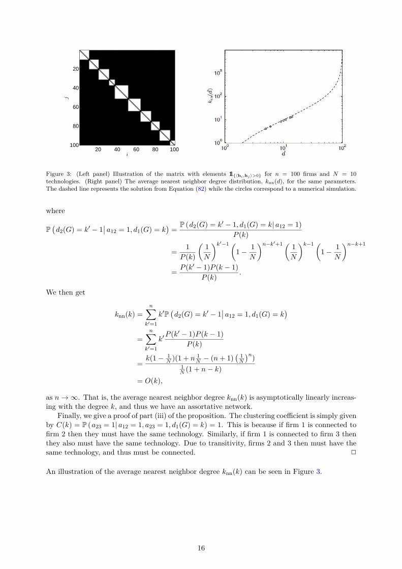
i
j
20 40 60 80 100
20
40
60
80
100
Figure 3: (Left panel) Illustration of the matrix with elements 1⟨hi,hj⟩>0 for n = 100 firms and N = 10technologies. (Right panel) The average nearest neighbor degree distribution, knn(d), for the same parameters.The dashed line represents the solution from Equation (82) while the circles correspond to a numerical simulation.
where
P(d2(G) = k′ − 1
∣∣ a12 = 1, d1(G) = k)=
P (d2(G) = k′ − 1, d1(G) = k| a12 = 1)
P (k)
=1
P (k)
(1
N
)k′−1(1− 1
N
)n−k′+1( 1
N
)k−1(1− 1
N
)n−k+1
=P (k′ − 1)P (k − 1)
P (k).
We then get
knn(k) =n∑
k′=1
k′P(d2(G) = k′ − 1
∣∣ a12 = 1, d1(G) = k)
=n∑
k′=1
k′P (k′ − 1)P (k − 1)
P (k)
=k(1− 1
N )(1 + n 1N − (n+ 1)
(1N
)n)
1N (1 + n− k)
= O(k),
as n→ ∞. That is, the average nearest neighbor degree knn(k) is asymptotically linearly increas-ing with the degree k, and thus we have an assortative network.
Finally, we give a proof of part (iii) of the proposition. The clustering coefficient is simply givenby C(k) = P (a23 = 1| a12 = 1, a23 = 1, d1(G) = k) = 1. This is because if firm 1 is connected tofirm 2 then they must have the same technology. Similarly, if firm 1 is connected to firm 3 thenthey also must have the same technology. Due to transitivity, firms 2 and 3 then must have thesame technology, and thus must be connected. 2
An illustration of the average nearest neighbor degree knn(k) can be seen in Figure 3.
16
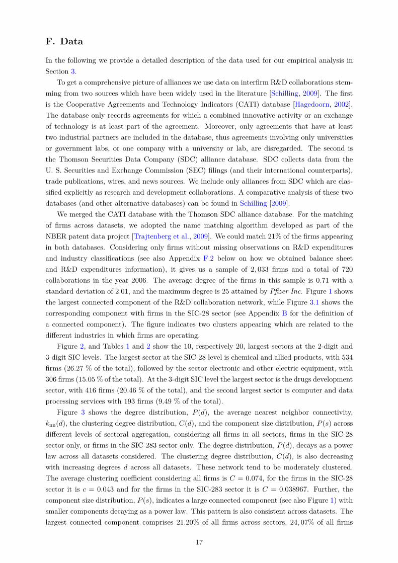
F. Data
In the following we provide a detailed description of the data used for our empirical analysis inSection 3.
To get a comprehensive picture of alliances we use data on interfirm R&D collaborations stem-ming from two sources which have been widely used in the literature [Schilling, 2009]. The firstis the Cooperative Agreements and Technology Indicators (CATI) database [Hagedoorn, 2002].The database only records agreements for which a combined innovative activity or an exchangeof technology is at least part of the agreement. Moreover, only agreements that have at leasttwo industrial partners are included in the database, thus agreements involving only universitiesor government labs, or one company with a university or lab, are disregarded. The second isthe Thomson Securities Data Company (SDC) alliance database. SDC collects data from theU. S. Securities and Exchange Commission (SEC) filings (and their international counterparts),trade publications, wires, and news sources. We include only alliances from SDC which are clas-sified explicitly as research and development collaborations. A comparative analysis of these twodatabases (and other alternative databases) can be found in Schilling [2009].
We merged the CATI database with the Thomson SDC alliance database. For the matchingof firms across datasets, we adopted the name matching algorithm developed as part of theNBER patent data project [Trajtenberg et al., 2009]. We could match 21% of the firms appearingin both databases. Considering only firms without missing observations on R&D expendituresand industry classifications (see also Appendix F.2 below on how we obtained balance sheetand R&D expenditures information), it gives us a sample of 2, 033 firms and a total of 720
collaborations in the year 2006. The average degree of the firms in this sample is 0.71 with astandard deviation of 2.01, and the maximum degree is 25 attained by Pfizer Inc. Figure 1 showsthe largest connected component of the R&D collaboration network, while Figure 3.1 shows thecorresponding component with firms in the SIC-28 sector (see Appendix B for the definition ofa connected component). The figure indicates two clusters appearing which are related to thedifferent industries in which firms are operating.
Figure 2, and Tables 1 and 2 show the 10, respectively 20, largest sectors at the 2-digit and3-digit SIC levels. The largest sector at the SIC-28 level is chemical and allied products, with 534firms (26.27 % of the total), followed by the sector electronic and other electric equipment, with306 firms (15.05 % of the total). At the 3-digit SIC level the largest sector is the drugs developmentsector, with 416 firms (20.46 % of the total), and the second largest sector is computer and dataprocessing services with 193 firms (9.49 % of the total).
Figure 3 shows the degree distribution, P (d), the average nearest neighbor connectivity,knn(d), the clustering degree distribution, C(d), and the component size distribution, P (s) acrossdifferent levels of sectoral aggregation, considering all firms in all sectors, firms in the SIC-28sector only, or firms in the SIC-283 sector only. The degree distribution, P (d), decays as a powerlaw across all datasets considered. The clustering degree distribution, C(d), is also decreasingwith increasing degrees d across all datasets. These network tend to be moderately clustered.The average clustering coefficient considering all firms is C = 0.074, for the firms in the SIC-28sector it is c = 0.043 and for the firms in the SIC-283 sector it is C = 0.038967. Further, thecomponent size distribution, P (s), indicates a large connected component (see also Figure 1) withsmaller components decaying as a power law. This pattern is also consistent across datasets. Thelargest connected component comprises 21.20% of all firms across sectors, 24, 07% of all firms
17
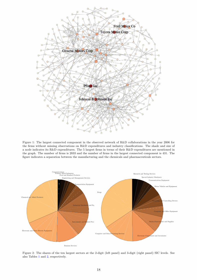
Figure 1: The largest connected component in the observed network of R&D collaborations in the year 2006 forthe firms without missing observations on R&D expenditures and industry classifications. The shade and size ofa node indicates its R&D expenditures. The 5 largest firms in terms of their R&D expenditures are mentioned inthe graph. The number of firms is 2033 and the number of firms in the largest connected component is 431. Thefigure indicates a separation between the manufacturing and the chemicals and pharmaceuticals sectors.
!"#$%&' &() *''$") +,-).%/0
1'"%/,-($% &() 2/!", 1'"%/,$% 13.$4#"(/
5.0$("00 6",7$%"0
8(0/,.#"(/0 &() 9"'&/") +,-).%/0
8().0/,$&' :&%!$(",; &() 13.$4#"(/
<,&(04-,/&/$-( 13.$4#"(/
1(=$("",$(= &() :&(&="#"(/ 6",7$%"0
>--) &() ?$(),") +,-).%/0+,$#&,; :"/&' 8().0/,$"0
-##.($%&/$-(0
!"#$
%&'(")*! +,- +)+ .!&/*$$0,# 1*!20/*$
34*/)!&,0/ %&'(&,*,)$ +,- 5//*$$&!0*$
6*-0/+4 7,$)!"'*,)$ +,- 1"((40*$
%&'(")*! +,- 8 /* 39"0('*,)
6*+$"!0,# +,- %&,)!&440,# *20/*$
6&)&! :*;0/4*$ +,- 39"0('*,)
%&''",0/+)0&,$ 39"0('*,)
1(*/0+4 7,-"$)!< 6+/;0,*!<
=*$*+!/; +,- >*$)0,# 1*!20/*$
Figure 2: The shares of the ten largest sectors at the 2-digit (left panel) and 3-digit (right panel) SIC levels. Seealso Tables 1 and 2, respectively.
18

Table 1: The 20 largest sectors at the 2-digit SIC level.
Sector 2-dig SIC # firms % of tot. Rank
Chemical and Allied Products 28 534 26.27 1Electronic and Other Electric Equipment 36 306 15.05 2Business Services 73 205 10.08 3Instruments and Related Products 38 204 10.03 4Industrial Machinery and Equipment 35 188 9.25 5Transportation Equipment 37 91 4.48 6Engineering and Management Services 87 59 2.90 7Food and Kindred Products 20 41 2.02 8Primary Metal Industries 33 39 1.92 9Communications 48 30 1.48 10Electric Gas and Sanitary Services 49 24 1.18 11Fabricated Metal Products 34 21 1.03 12Health Services 80 20 0.98 13Miscellaneous Manufacturing Industries 39 18 0.89 14Paper and Allied Products 26 16 0.79 15Rubber and Miscellaneous Plastics Products 30 16 0.74 16Petroleum and Coal Products 29 14 0.69 17Stone Clay and Glass Products 32 14 0.69 18Wholesale Trade - Durable Goods 50 13 0.64 19Textile Mill Products 22 12 0.59 20
Table 2: The 20 largest sectors at the 3-digit SIC level.
Sector 3-dig SIC # firms % of tot. Rank
Drugs 283 416 20.46 1Computer and Data Processing Services 737 193 9.49 2Electronic Components and Accessories 367 156 7.67 3Medical Instruments and Supplies 384 99 4.87 4Computer and Office Equipment 357 72 3.54 5Measuring and Controlling Devices 382 72 3.54 6Motor Vehicles and Equipment 371 67 3.30 7Communications Equipment 366 61 3.00 8Special Industry Machinery 355 38 1.87 9Research and Testing Services 873 37 1.82 10Misc. Electrical Equipment and Supplies 369 28 1.38 11Chemicals & Allied Products 280 26 1.28 12Plastics Materials and Synthetic 282 25 1.23 13General Industrial Machinery 356 25 1.23 14Electrical Industrial Apparatus 362 17 0.84 15Aircraft and Parts 372 16 0.79 16Misc. Chemical Products 289 15 0.74 17Blast Furnace and Basic Steel Products 331 15 0.74 18Agricultural Chemicals 287 14 0.69 19Metalworking Machinery 354 14 0.69 20
19
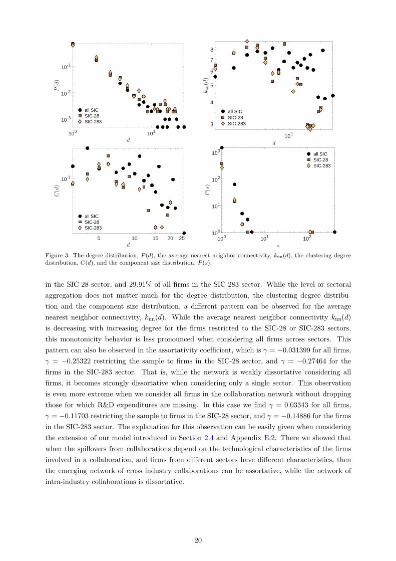
100 101
d
10-3
10-2
10-1
P(d)
all SICSIC-28SIC-283
101
d
3
4
5
6
7
8
knn(d)
all SICSIC-28SIC-283
5 10 15 20 25d
10-1
C(d)
all SICSIC-28SIC-283
100 101 102
s
100
101
102
103
P(s)
all SICSIC-28SIC-283
Figure 3: The degree distribution, P (d), the average nearest neighbor connectivity, knn(d), the clustering degreedistribution, C(d), and the component size distribution, P (s).
in the SIC-28 sector, and 29.91% of all firms in the SIC-283 sector. While the level or sectoralaggregation does not matter much for the degree distribution, the clustering degree distribu-tion and the component size distribution, a different pattern can be observed for the averagenearest neighbor connectivity, knn(d). While the average nearest neighbor connectivity knn(d)
is decreasing with increasing degree for the firms restricted to the SIC-28 or SIC-283 sectors,this monotonicity behavior is less pronounced when considering all firms across sectors. Thispattern can also be observed in the assortativity coefficient, which is γ = −0.031399 for all firms,γ = −0.25322 restricting the sample to firms in the SIC-28 sector, and γ = −0.27464 for thefirms in the SIC-283 sector. That is, while the network is weakly dissortative considering allfirms, it becomes strongly dissortative when considering only a single sector. This observationis even more extreme when we consider all firms in the collaboration network without droppingthose for which R&D expenditures are missing. In this case we find γ = 0.03343 for all firms,γ = −0.11703 restricting the sample to firms in the SIC-28 sector, and γ = −0.14886 for the firmsin the SIC-283 sector. The explanation for this observation can be easily given when consideringthe extension of our model introduced in Section 2.4 and Appendix E.2. There we showed thatwhen the spillovers from collaborations depend on the technological characteristics of the firmsinvolved in a collaboration, and firms from different sectors have different characteristics, thenthe emerging network of cross industry collaborations can be assortative, while the network ofintra-industry collaborations is dissortative.
20
F.1. Mergers and Acquisitions
Some firms might be acquired by other firms due to mergers and acquisitions (M&A) over time,and this will impact the R&D collaboration network [Hanaki et al., 2010].
To get a comprehensive picture of the M&A activities of the firms in our dataset, we use twoextensive datasources to obtain information about M&As. The first is the Thomson Reuters’Securities Data Company (SDC) M&A database, which has historically been the most widelyused database for empirical research in the field of M&As. Data in SDC dates back to 1965with a slightly more complete coverage of deals starting in the early 1980s. The second databasewith information about M&As is Bureau van Dijk’s (BvD) Zephyr database, which is a recentalternative to the SDC M&As database. The history of deals recorded in Zephyr goes back to1997. In 1997 and 1998 only European deals are recorded, while international deals are includedstarting from 1999. According to Huyghebaert and Luypaert [2010], Zephyr “covers deals ofsmaller value and has a better coverage of European transactions”. A comparison and moredetailed discussion of the two databases can be found in Bollaert and Delanghe [2015] and Benaet al. [2008].
We merged the SDC and Zephyr databases (with the above mentioned name matching al-gorithm; see also Trajtenberg et al. [2009]) to obtain information on M&As of 116, 641 uniquefirms. Using the same name matching algorithm we could identify 43.08% of the firms in thecombined CATI-SDC alliance database that also appear in the combined SDC-Zephyr M&Asdatabase. We then account for the M&A activities of these matched firms when constructing theR&D collaboration network by assuming that an acquiring firm in a M&A inherits all the R&Dcollaborations of the target firm, and we remove the target firm form from the network.
F.2. Balance Sheet Statements, R&D and Productivity
The combined CATI-SDC alliance database provides the names for each firm in an alliance, butit does not contain information about the firms’ output levels or R&D expenses. We thereforematched the firms’ names in the combined CATI-SDC database with the firms’ names in Stan-dard & Poor’s Compustat U.S. and Global fundamentals annual databases and Bureau van Dijk(BvD)’s Orbis database, to obtain information about their balance sheets and income statements.
Compustat North America is a database of U.S. and Canadian active and inactive publiclyheld companies extracted from company filings. It provides more than 300 annual and 100quarterly income statements, balance sheets and statement of cash flows. Compustat Global isa database of non-U.S. and non-Canadian companies and contains market information on morethan 33,900 active and inactive publicly held companies with annual data history from 1987. TheCompustat databases cover 99% of the world’s total market capitalization with annual companydata history available back to 1950. The databases contains only firms listed on the stock market,so it typically excludes smaller private firms, but this is inevitable if one is going to use marketvalue data. Nevertheless, R&D is concentrated in publicly listed firms, and it thus covers mostof the R&D activities in the economy [Bloom et al., 2013].
The Orbis database is owned by Bureau van Dijk (BvD). It is a commercial dataset, whichcontains administrative data on 130 million firms worldwide. Orbis is an umbrella product thatprovides firm-level data covering over 120 countries, both developed and emerging, since 2005.The financial and balance-sheet information in Orbis comes from business registers collected by
21
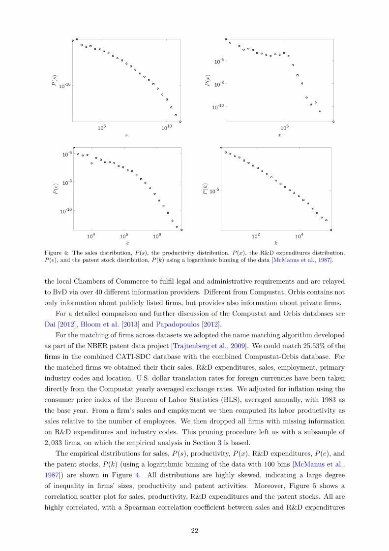
105 1010
s
10-10P(s)
105
x
10-10
10-8
10-6
P(x)
104 106 108
e
10-10
10-8
10-6
P(e)
102 104
k
10-5
P(k)
Figure 4: The sales distribution, P (s), the productivity distribution, P (x), the R&D expenditures distribution,P (e), and the patent stock distribution, P (k) using a logarithmic binning of the data [McManus et al., 1987].
the local Chambers of Commerce to fulfil legal and administrative requirements and are relayedto BvD via over 40 different information providers. Different from Compustat, Orbis contains notonly information about publicly listed firms, but provides also information about private firms.
For a detailed comparison and further discussion of the Compustat and Orbis databases seeDai [2012], Bloom et al. [2013] and Papadopoulos [2012].
For the matching of firms across datasets we adopted the name matching algorithm developedas part of the NBER patent data project [Trajtenberg et al., 2009]. We could match 25.53% of thefirms in the combined CATI-SDC database with the combined Compustat-Orbis database. Forthe matched firms we obtained their their sales, R&D expenditures, sales, employment, primaryindustry codes and location. U.S. dollar translation rates for foreign currencies have been takendirectly from the Compustat yearly averaged exchange rates. We adjusted for inflation using theconsumer price index of the Bureau of Labor Statistics (BLS), averaged annually, with 1983 asthe base year. From a firm’s sales and employment we then computed its labor productivity assales relative to the number of employees. We then dropped all firms with missing informationon R&D expenditures and industry codes. This pruning procedure left us with a subsample of2, 033 firms, on which the empirical analysis in Section 3 is based.
The empirical distributions for sales, P (s), productivity, P (x), R&D expenditures, P (e), andthe patent stocks, P (k) (using a logarithmic binning of the data with 100 bins [McManus et al.,1987]) are shown in Figure 4. All distributions are highly skewed, indicating a large degreeof inequality in firms’ sizes, productivity and patent activities. Moreover, Figure 5 shows acorrelation scatter plot for sales, productivity, R&D expenditures and the patent stocks. All arehighly correlated, with a Spearman correlation coefficient between sales and R&D expenditures
22
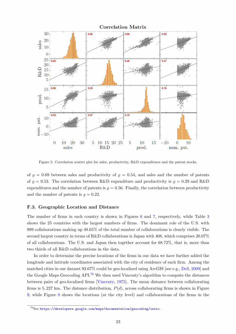
Figure 5: Correlation scatter plot for sales, productivity, R&D expenditures and the patent stocks.
of ϱ = 0.69 between sales and productivity of ϱ = 0.54, and sales and the number of patentsof ϱ = 0.53. The correlation between R&D expenditure and productivity is ϱ = 0.29 and R&Dexpenditures and the number of patents is ϱ = 0.56. Finally, the correlation between productivityand the number of patents is ϱ = 0.22.
F.3. Geographic Location and Distance
The number of firms in each country is shown in Figures 6 and 7, respectively, while Table 3shows the 25 countries with the largest numbers of firms. The dominant role of the U.S. with989 collaborations making up 48.65% of the total number of collaborations is clearly visible. Thesecond largest country in terms of R&D collaborations is Japan with 408, which comprises 20.07%of all collaborations. The U.S. and Japan then together account for 68.72%, that is, more thantwo thirds of all R&D collaborations in the data.
In order to determine the precise locations of the firms in our data we have further added thelongitude and latitude coordinates associated with the city of residence of each firm. Among thematched cities in our dataset 93.67% could be geo-localized using ArcGIS [see e.g., Dell, 2009] andthe Google Maps Geocoding API.76 We then used Vincenty’s algorithm to compute the distancesbetween pairs of geo-localized firms [Vincenty, 1975]. The mean distance between collaboratingfirms is 5, 227 km. The distance distribution, P (d), across collaborating firms is shown in Figure9, while Figure 8 shows the locations (at the city level) and collaborations of the firms in the
76See https://developers.google.com/maps/documentation/geocoding/intro.
23
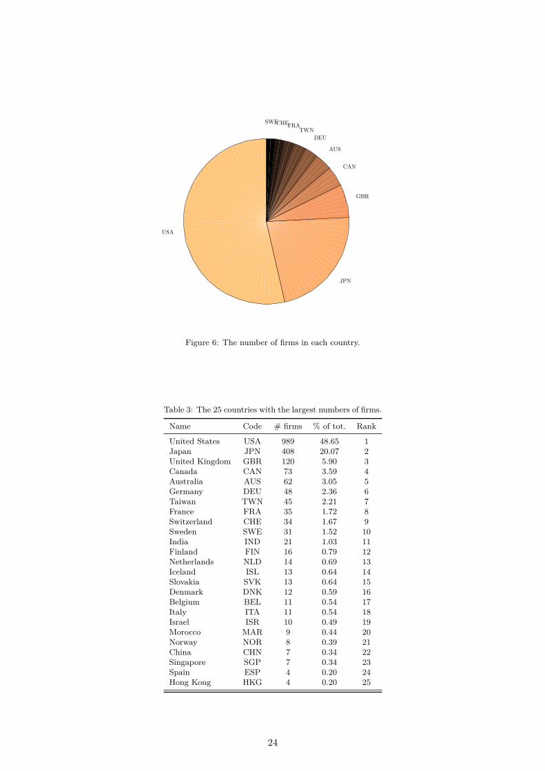
USA
JPN
GBR
CAN
AUS
DEU
TWNFRA
CHESWE
Figure 6: The number of firms in each country.
Table 3: The 25 countries with the largest numbers of firms.
Name Code # firms % of tot. Rank
United States USA 989 48.65 1Japan JPN 408 20.07 2United Kingdom GBR 120 5.90 3Canada CAN 73 3.59 4Australia AUS 62 3.05 5Germany DEU 48 2.36 6Taiwan TWN 45 2.21 7France FRA 35 1.72 8Switzerland CHE 34 1.67 9Sweden SWE 31 1.52 10India IND 21 1.03 11Finland FIN 16 0.79 12Netherlands NLD 14 0.69 13Iceland ISL 13 0.64 14Slovakia SVK 13 0.64 15Denmark DNK 12 0.59 16Belgium BEL 11 0.54 17Italy ITA 11 0.54 18Israel ISR 10 0.49 19Morocco MAR 9 0.44 20Norway NOR 8 0.39 21China CHN 7 0.34 22Singapore SGP 7 0.34 23Spain ESP 4 0.20 24Hong Kong HKG 4 0.20 25
24

[0,1] [1,2] [2,5] [5,13] [13,31] [31,74] [74,176] [176,417] [417,988]
Figure 7: The number of firms in each country.
database. The distance distribution, P (d), is heavily skewed. We find that R&D collaborationstend to be more likely between firms that are close, showing that geography matters for R&Dcollaborations and this spillovers, in line with previous empirical studies [Lychagin et al., 2016].
F.4. Patents and Technological Similarity
We identified the patent portfolios of the firms in our dataset using the EPO Worldwide PatentStatistical Database (PATSTAT) [Jaffe and Trajtenberg, 2002; Thoma et al., 2010]. It includesbibliographic details on patents filed to 80 patent offices worldwide, covering more than 60 milliondocuments. Hence filings in all major countries and the the World International Patent Office arecovered. We matched the firms in our data with the assignees in the PATSTAT database usingthe above mentioned name matching algorithm. We only consider granted patents (or successfulpatents), as opposed to patents applied for, as they are the main drivers of revenue derived fromR&D [Copeland and Fixler, 2012]. We obtained matches for roughly 30% of the firms in the data.The technology classes were identified using the main international patent classification (IPC)numbers at the 4 digit level.
The technological proximity fkij = fkji, k ∈ J,M (see Equation (23)), between firms i and j
is measured with two alternative metrics. The first, fJij , is based on Jaffe [1989]. Let Pi representsthe patent portfolio of firm i, where, for each firm i, Pi is a vector whose k-th component, Pik,counts the number of patents firm i has in technology category k divided by the total number oftechnologies attributed to the firm [see also Bloom et al., 2013]. The technological proximity offirm i and j is then given by
fJij =P⊤i Pj√
P⊤i Pi
√P⊤j Pj
. (83)
25

Figure 8: The locations (at the city level) and collaborations of the firms in the combined CATI-SDC database.
We denote by FJ the (n× n) matrix with elements (fJij)1≤i,j≤n.As an alternative measure for technological similarity we also consider the Mahalanobis tech-
nology proximity measure, fMij , introduced by Bloom et al. [2013]. To construct this metric, letN be the number of technology classes, n the number of firms, and let T be the (N × n) patentshares matrix with elements Tji = Pji/
∑nk=1 Pki, for all 1 ≤ i ≤ n and 1 ≤ j ≤ N . Further, we
construct the (N × n) normalized patent shares matrix T with elements Tji = Tji/√∑N
k=1 T2ki,
and the (n × N) normalized patent shares matrix across firms is defined by X with elementsXik = Tki/
√∑Ni=1 T
2ki. Let Ω = X⊤X. Then the (n × n) Mahalanobis technology similarity
matrix FM = (fMij )1≤i,j≤n is defined as
FM = T⊤ΩT. (84)
We then use either fJij or fMij as a measure for the potential technology spillovers between col-laborating firms in the profit function of Equation (23). Both measures are highly correlated.The Spearman correlation coefficient between the Jaffe and the Mahalanobis proximity metricsis 0.91882, and a correlation plot can be seen in the right panel of Figure 9.
G. Estimation Algorithms
In the following appendices we provide additional details regarding our estimation algorithms.First, in Appendix G.1 we give a detailed explanation for how the DMH algorithm is implemented.Second, in Appendix G.2 we discuss the implementation of the AEX algorithm. Further, inAppendix G.3 we outline the convergence proof of the AEX algorithm.
G.1. Implementation of the DMH Algorithm
In our empirical model, the unknown parameters are denoted by θ = (ρ, b, δ⊤,γ⊤,κ), where ρcaptures the technology spillover effect; b captures the competition effect; δ captures effects offirm’s exogenous characteristics in terms of productivity and sector fixed effect; γ captures effects
26
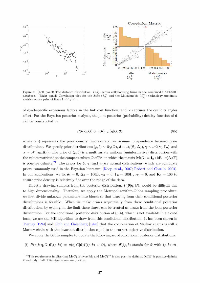
102
104
106
108
10−9
10−8
10−7
10−6
10−5
10−4
d
P(d
)
Figure 9: (Left panel) The distance distribution, P (d), across collaborating firms in the combined CATI-SDCdatabase. (Right panel) Correlation plot for the Jaffe (fJ
ij) and the Mahalanobis (fMij ) technology proximity
metrics across pairs of firms 1 ≤ i, j ≤ n.
of dyad-specific exogenous factors in the link cost function; and κ captures the cyclic triangleseffect. For the Bayesian posterior analysis, the joint posterior (probability) density function of θcan be constructed by
P (θ|q, G) ∝ π(θ) · µ(q|G,θ), (85)
where π(·) represents the prior density function and we assume independence between priordistributions. We specify prior distributions (ρ, b) ∼ U2(O), δ ∼ Nl(δ0,∆0), γ ∼ Nr(γ0,Γ0), andκ ∼ N (κ0,K0). The prior of (ρ, b) is a multivariate uniform (uninformative) distribution withthe values restricted to the compact subset O of R2, in which the matrix M(G) = In+bB−ρ(AF)is positive definite.77 The priors for δ, γ, and κ are normal distributions, which are conjugatepriors commonly used in the Bayesian literature [Koop et al., 2007; Robert and Casella, 2004].In our applications, we fix δ0 = 0, ∆0 = 100Il, γ0 = 0, Γ0 = 100Ir, κ0 = 0, and K0 = 100 toensure prior density is relatively flat over the range of the data.
Directly drawing samples from the posterior distribution, P (θ|q, G), would be difficult dueto high dimensionality. Therefore, we apply the Metropolis-within-Gibbs sampling procedure:we first divide unknown parameters into blocks so that drawing from their conditional posteriordistributions is feasible. When we make draws sequentially from these conditional posteriordistributions by cycling, in the limit these draws can be treated as draws from the joint posteriordistribution. For the conditional posterior distribution of (ρ, b), which is not available in a closedform, we use the MH algorithm to draw from this conditional distribution. It has been shown inTierney [1994] and Chib and Greenberg [1996] that the combination of Markov chains is still aMarkov chain with the invariant distribution equal to the correct objective distribution.
We apply the Gibbs sampler to update the following set of conditional posterior distributions:
(i) P (ρ, b|q, G,θ\(ρ, b)) ∝ µ(q, G|θ)I((ρ, b) ∈ O), where θ\(ρ, b) stands for θ with (ρ, b) ex-
77This requirement implies that M(G) is invertible and M(G)−1 is also positive definite. M(G) is positive definiteif and only if all of its eigenvalues are positive.
27
cluded.
(ii) P (δ|q, G,θ\δ) ∝ ϕl(δ; δ0,∆0) · µ(q|G,θ), where ϕ denotes the normal density function.
(iii) P (γ|q, G,θ\γ) ∝ ϕr(γ;γ0,Γ0) · µ(q, G|θ).
(iv) P (κ|q, G,θ\κ) ∝ ϕ(κ;κ0,K0) · µ(q, G|θ).
We apply the DMH algorithm to simulate draws from (i) to (iv) because their distributionsare not available in a closed form. At each tth MCMC iteration, the implementation steps areillustrated as follows:
Step I. Simulate (ρ(t), b(t)) from P(ρ, b∣∣q, G,Υ(t−1)
)by the DMH algorithm, where Υ(t−1) denotes
the rest of parameters evaluated at the (t− 1)th iteration.
(a) propose (ρ, b) from a random walk proposal density T1(ρ, b|b(t−1), ρ(t−1)).
(b) simulate an auxiliary data q′ and G′ by M runs of the MH algorithm based on
µ(q, G|ρ, b,Υ(t−1)) =exp
(Φ(q, G, ρ, b,Υ(t−1)
))∑
g∈Gn
∫Qn exp
(Φ(q, g, ρ, b,Υ(t−1)
))dq
starting from the observed network G.78 The details are as follows:First, let the initial auxiliary network G(0) equal to the observed network G, i.e., set theauxiliary adjacency matrix A(0) = A. At the mth run, m = 1, · · · ,M , we propose G
from G(m−1) by selecting node i with probability 1n and node j = i with a probability
1n−1 randomly and change the value a(m−1)
ij and a(m−1)ji in matrix A(m−1) to 1 − a
(m−1)ij
and 1 − a(m−1)ji and propose it as A. With a certain probability, we flip all elements in
A(m−1) from 0 to 1 (or 1 to 0) and propose it as A. Denote M = In + bB− ρ(A F) andcalculate q∗ = M−1
(Xδ(t−1)
). Simulate q from Nn
(q∗, M−1
). Then, with the acceptance
probability
α(G|G(m−1)) = min
exp(Φ(G, q)
)exp
(Φ(G(m−1),q(m−1))
) , 1 ,
set G(m) to G and q(m) = q, otherwise, set G(m) = G(m−1) and q(m) = q(m−1). After theM runs, collect G′(M) and q′ = q(M).
(c) With the acceptance probability equals to
α(ρ, b|ρ(t−1), b(t−1), G′,q′)
= min
µ(q, G,Υ(t−1), ρ, b
)µ (q, G,Υ(t−1), ρ(t−1), b(t−1))
·µ(q′, G′(t−1), ρ(t−1), b(t−1)
)µ(q′, G′(t−1), ρ, b
) · I((ρ, b) ∈ O)
I((ρ(t−1), b(t−1)) ∈ O), 1
= min
exp(Φ(q, G,Υ(t−1), ρ, b)
)exp (Φ(q, G,Υ(t−1), ρ(t−1), b(t−1)))
·exp
(Φ(q′, G′(t−1), ρ(t−1), b(t−1))
)exp
(Φ(q′, G′(t−1), ρ, b)
) · I((ρ, b) ∈ O)
I((ρ(t−1), b(t−1)) ∈ O), 1
,
78This step mimics the MH sampler in Snijders [2002] and Mele [2017]. In practice, we set M = n2 where n isthe size of the network.
28

set (ρ(t), b(t)) = (ρ, b). Otherwise, set (ρ(t), b(t)) = (ρ(t−1), b(t−1)).
Step II. Simulate δ(t) from
P (δ|q, G, ρ(t), b(t),Υ(t−1)) ∝ ϕl(δ; δ0,∆0) · µ(q|G, ρ(t), b(t), δ,Υ(t−1)).
(a) propose δ from a random walk proposal density T2(δ|δ(t−1)).
(b) simulate an auxiliary data q′ and G′ by M runs of the MH algorithm based on
µ(q, G|δ, ρ(t), b(t),Υ(t−1)) =exp
(Φ(q, G, δ, ρ(t), b(t),Υ(t−1)
))∑
g∈Gn
∫Qn exp
(Φ(q, g, δ, ρ(t), b(t),Υ(t−1)
))dq
starting from the observed network G.
(c) With the acceptance probability equals to
α(δ|δ(t−1), G′,q′)
= min
µ(q, G, δ,Υ(t−1), ρ(t), b(t)
)µ (q, G, δ(t−1),Υ(t−1), ρ(t), b(t))
·µ(q′, G′, δ(t−1),Υ(t−1), ρ(t), b(t)
)µ(q′, G′, δ,Υ(t−1), ρ(t), b(t)
) · ϕl(δ; δ0,∆0)
ϕl(δ(t−1); δ0,∆0), 1
= min
exp(Φ(q, G, δ,Υ(t−1), ρ(t), b(t))
)exp (Φ(q, G, δ(t−1),Υ(t−1), ρ(t), b(t)))
·exp
(Φ(q′, G′, δ(t−1),Υ(t−1), ρ(t), b(t))
)exp
(Φ(q′, G′, δ,Υ(t−1), ρ(t), b(t))
) · ϕl(δ; δ0,∆0)
ϕl(δ(t−1); δ0,∆0), 1
,
set δ(t) = δ. Otherwise, set δ(t) = δ(t−1).
Step III. Simulate γ(t) from P(γ∣∣q, G,Υ(t−1), δ(t), ρ(t), b(t)
)by the DMH algorithm.
(a) propose γ from a random walk proposal density T3(γ|γ(t−1))
(b) simulate an auxiliary data q′ and G′ by M runs of the MH algorithm based on
µ(q, G|γ,Υ(t−1), δ(t), ρ(t), b(t)) =exp
(Φ(q, G, γ,Υ(t−1), δ(t), ρ(t), b(t)
))∑g∈Gn
∫Qn exp
(Φ(q, g, γ,Υ(t−1), δ(t), ρ(t), b(t)
))dq
starting from the observed network G.
(d) With the acceptance probability equal to
α(γ|γ(t−1), G′,q′)
= min
µ(G,q, γ,Υ(t−1), δ(t), ρ(t), b(t)
)µ (G,q,γ(t−1),Υ(t−1), δ(t), ρ(t), b(t))
·µ(G′,q′,γ(t−1),Υ(t−1), δ(t), ρ(t), b(t)
)µ (G′,q′, γ,Υ(t−1), δ(t), ρ(t), b(t))
· ϕr(γ|γ0,Γ0)
ϕr(γ(t−1)|γ0,Γ0), 1
= min
exp(Φ(G,q, γ,Υ(t−1), δ(t), ρ(t), b(t))
)exp (Φ(G,q,γ(t−1),Υ(t−1), δ(t), ρ(t), b(t)))
·exp
(Φ(G′,q′,γ(t−1),Υ(t−1), δ(t), ρ(t), b(t))
)exp (Φ(G′,q′, γ,Υ(t−1), δ(t), ρ(t), b(t)))
· ϕr(γ|γ0,Γ0)
ϕr(γ(t−1)|γ0,Γ0), 1
,
set γ(t) = γ. Otherwise, set γ(t) = γ(t−1).
29
Step IV. Simulate κ(t) from P(κ∣∣q, G,γ(t), δ(t), ρ(t), b(t)
)by the DMH algorithm.
(a) propose κ from a random walk proposal density T4(κ|κ(t−1))
(b) simulate an auxiliary data q′ and G′ by M runs of the MH algorithm based on
µ(q, G|κ,γ(t), δ(t), ρ(t), b(t)) =exp
(Φ(q, G, κ,γ(t), δ(t), ρ(t), b(t)
))∑g∈Gn
∫Qn exp
(Φ(q, g, κ,γ(t), δ(t), ρ(t), b(t)
))dq
starting from the observed network G.
(d) With the acceptance probability equal to
α(κ|κ(t−1), G′,q′)
= min
µ(G,q, κ,γ(t), δ(t), ρ(t), b(t)
)µ (G,q,κ(t−1),γ(t), δ(t), ρ(t), b(t))
·µ(G′,q′(t−1),γ(t), δ(t), ρ(t), b(t)
)µ (G′,q′, κ,γ(t), δ(t), ρ(t), b(t))
· ϕr(κ|κ0,K0)
ϕr(κ(t−1)|κ0,K0), 1
= min
exp(Φ(G,q, κ,γ(t), δ(t), ρ(t), b(t))
)exp (Φ(G,q,κ(t−1),γ(t), δ(t), ρ(t), b(t)))
·exp
(Φ(G′,q′(t−1),γ(t), δ(t), ρ(t), b(t))
)exp (Φ(G′,q′, κ,γ(t), δ(t), ρ(t), b(t)))
· ϕr(κ|κ0,K0)
ϕr(κ(t−1)|κ0,K0), 1
,
set γ(t) = γ. Otherwise, set γ(t) = γ(t−1).
G.2. Implementation of the AEX Algorithm
The AEX algorithm consists of two Markov chains running in parallel. Let the subscript t denotethe tth iteration of two chains. In the first chain, we simulate auxiliary network and outputsample (G(t), q(t)) from µ(G, q|θ(t)), where θ(t) is sampled from the set of pre-specified parameterpoints (θ1, · · · ,θm). In our applications, we set m = 50 and (θ1, · · · ,θm) are chosen from theDMH draws using the Max-Min procedure suggested in Liang et al. [2015]. The index functionH(θ(t)) denotes the order index of θ(t), i.e., H(θ(t)) = i if θ(t) = θi. Let p = (p1, · · · , pm) be thedesired sampling frequencies from the respective distributions µ(G, q|θ1), · · · , µ(G, q|θm), where0 < pi < 1 and
∑mi=1 pi = 1. We follow Liang et al. [2015] to set p1 = · · · = pm = 1
m . Asrequired by the SAMC algorithm, we specify a gain factor sequence, at, which is a positive,nonincreasing sequence satisfying the following condition:
(A1) limt→∞ at = 0,∑∞
t=1 at = ∞,∑∞
t=1 akt <∞ for some k ∈ (1, 2].
Following Liang et al. [2015], we set at = t0max(t0,t)
with a known constant t0 > 1. Since a largervalue of t0 will help the auxiliary chain to reach each distribution µ(G, q|θi) more quickly, weset t0 = 20, 000 in this paper. Also, we let w(t)
i denote an abundance factor attached to each dis-tribution µ(G, q|θi) at iteration t and w(t) = (w
(t)1 , · · · , w(t)
m ). We set the initial values w(0)1 = · · · =
w(0)m = 1 in the simulation. Finally, let Ω(t)= (G(1), · · · , G(t), q(1), · · · , q(t),θ(1), · · · , θ(t),H(θ(1)), · · · ,H(θ(t)),
w(1), · · · , w(t)) denote the information in the auxiliary chain that we collect up to iteration t. Inthe second chain, we draw θ(t) by the exchange algorithm from the target posterior distribu-tion µ(θ|q, G). Explicitly, the AEX algorithm is implemented by Part I and Part II at each tth
iteration described as follows:
Part I. Auxiliary network simulation
30
1. Choose to update θ(t) or G(t) with a pre-specified probability. In our application, wechoose 75% for updating θ(t) and 25% for updating G(t).
(a) Update θ(t): Select θ′ from the set (θ1, · · · ,θm) according to a proposal distribu-tion T1(·|θ(t−1)). With the probability
α(θ′∣∣∣θ(t−1)
)= min
w(t−1)
H(θ(t−1))exp(Φ(G(t−1), q(t−1), θ′))T1(θ
(t−1)|θ′)
w(t−1)
H(θ′)exp(Φ(G(t−1), q(t−1), θ(t−1)))T1(θ′|θ(t−1))
, 1
,
(86)
update (θ(t), G(t), q(t)) = (θ′, G(t−1), q(t−1)). Otherwise,set (θ(t), G(t), q(t)) = (θ(t−1), G(t−1), q(t−1)).
(b) Update (G(t), q(t)): simulate G(t) and q(t) from µ(G, q|θ(t−1)) via few MH updatesstarting from (G(t−1), q(t−1)). Then set θ(t) = θ(t−1).
2. For i = 1, · · · ,m, update the abundance factor w(t)i by
log(w(t)i ) = log(w
(t−1)i ) + at(ei,t − pi),
where ei,t = 1 if θ(t) = θi and 0 otherwise.
3. Append (θ(t), G(t), q(t),H(θ(t)), w(t)) to the collection Ω(t−1) to form Ω(t).
Part II. Adaptive Exchange algorithm for target parameter
4. Propose a candidate θ′ from a random walk proposal distribution T2(θ′|θ(t−1)).
5. Re-sample an auxiliary network and output data (G′,q′) from the collection Ω(t) via animportance sampling procedure. With the probability
P((G′,q′) = (G(i), q(i))
)=
∑tj=1
w
(j)
H(θ(j))
exp(Φ(G(j),q(j),θ′))
exp(Φ(G(j),q(j),θ(j)))I(G(j) = G(i)
)∑t
j=1
w
(j)
H(θ(j))
exp(Φ(Gj ,q(j),θ′))
exp(Φ(G(j),q(j),θ(j)))
, (87)
choose (G′,q′) = (G(i), q(i)), i ∈ (1, 2, · · · , t).6. Implement the exchange algorithm. With the probability
α(θ′|θ(t−1), G′,q′)
= min
exp(Φ(G,q,θ′))
exp(Φ(G,q,θ(t−1)))· exp(Φ(G
′,q′,θ(t−1)))
exp(Φ(G′,q′,θ′))· π(θ′)
π(θ(t−1)), 1
, (88)
set θ(t) = θ′. Otherwise, set θ(t) = θ(t−1).
G.3. Convergence of the AEX Algorithm
In this appendix, we outline the ideas and main results behind the convergence proof of the AEXalgorithm. Interested readers are referred to Jin et al. [2013] and the supplementary material ofLiang et al. [2015] for the completed version of proof. From Part II of the AEX algorithm, onecan see that auxiliary sample (G′,q′) is drawn via a dynamic importance sampling procedurein Equation (87), which implies that the underlying proposal distribution for auxiliary networkschanges from iteration to iteration. Therefore, AEX falls into the class of adaptive MCMC algo-rithms with varying stationary distributions and requires an unconventional convergence theory[Fort et al., 2011; Roberts and Rosenthal, 2007].
31

Liang et al. [2015] provided an ergodicity theorem for adaptive Markov chains with varyingstationary distributions, which can be used to prove ergodicity of the AEX algorithm. Considera state space, (X,H), where Xt ∈ X denotes the state of the Markov chain at iteration t andH denotes the Borel set defined on X. Let γt denote realization of the adoption index Γt ∈ Yand Ft = σ(X0, · · · , Xt,Γ0, · · · ,Γt) be the filtration generated by Xi,Γiti=0. Let Pγt denote thetransition kernel at iteration t and thus,
P (Xt+1 ∈ B|Xt = x,Γt = γt,Ft−1) = Pγt(x,B), x ∈ X, γt ∈ Y, B ∈ H.
Let P hγ (x,B) = Pγ(Xh ∈ B|X0 = x) denote the h-step transition probability for the Markov chainwith the fixed transition kernel Pγ and the initial condition X0 = x. Also let P h((x, γ), B) =
P (Xh ∈ B|X0 = x,Γ0 = γ,Fh−1), B ∈ H, denote the h-step transition probability for theadaptive Markov chain with the initial conditions X0 = x and Γ0 = γ. An adaptive Markovchain is called ergodic if limt→∞ V (x, γ, t) = 0 for all x ∈ X and γ ∈ Y, where
V (x, γ, t) =∥ P t((x, γ), ·)− π(·) ∥= supB∈H
∥ P t((x, γ), B)− π(B) ∥
denotes the total variation distance between the distribution of the adaptive chain at iteration t
and the target distribution π(·).
Theorem 2. Consider an adaptive Markov chain defined on the state space (X,H) with theadoption index Γt ∈ Y. The adoptive Markov chain is ergodic if the following conditions aresatisfied:
(a) (Stationarity) There exist a stationary distribution πγt(·) for each transition kernel Pγt.
(b) (Asymptotic Simultaneous Uniform Ergodicity) For any u > 0, there exist a measurable setE(u) in the probability space such that Pr(E(u)) ≥ 1 − u and on this set E(u), for anyϵ > 0, there exist t(ϵ) ∈ N and n(ϵ) ∈ N such that
supx∈X
∥ Pnγt(x, ·)− π(·) ∥≤ ϵ,
for all t > t(ϵ) and n > n(ϵ).
(c) (Diminishing Adoption) let Dt = supx∈X ∥ PΓt+1(x, ·) − PΓt(x, ·) ∥ and limt→∞Dt = 0 inprobability.
From conditions (a) and (b) of Theorem 2, it is implied that on the set E(u), for any ϵ,
∥ πγt(·)− π(·) ∥=∥ πγt(·)P hγt − π(·) ∥≤ supx∈X
∥ Pnγt(x, ·)− π(·) ∥≤ ϵ,
for t > t(ϵ) and n > n(ϵ). Furthermore, by the triangular inequality,
∥ Pnγt(x, ·)− πγt(·) ∥<∥ Pnγt(x, ·)− π(·) ∥ + ∥ πγt(·)− π(·) ∥< 2ϵ,
for t > t(ϵ) and n > n(ϵ). Thus, the simultaneous uniform ergodicity of Pγt on the set E(u) isestablished. Given condition (c) of Theorem 2 and the simultaneous uniform ergodicity of Pγt,Liang et al. [2015] show the weak law of large numbers for an adaptive Markov chain in thefollowing theorem:
32
Theorem 3. Consider an adaptive Markov chain defined on the state space (X,H). Let g(·) be abounded measurable function. Suppose that conditions (a), (b), and (c) of Theorem 2 hold, then1T
∑Tt=1 g(Xt) → π(g), in probability as T → ∞, where π(g) =
∫X g(x)π(dx).
The rest of procedure is to show the AEX algorithm satisfies three conditions of Theorem 2and thus it is ergodic and the weak law of large number holds for the average of sample pathθ(t). To begin with, we assume that in the auxiliary chain, the Markov transition kernel, Pw,for updating the state variable Xt = (G(t), q(t), θ(t)) ∈ X via the SAMC algorithm satisfies thefollowing Doeblin condition:
(A2) For any given w ∈ ϖ, the Markov transition kernel Pw is irreducible and aperiodic. Inaddition, there exist an integer h, a real number 0 < δ < 1, and a probability measure νsuch that for any compact subset K ⊂ ϖ,
infw∈K
P hw(x,B) ≥ δν(B), ∀x ∈ X, ∀B ∈ H,
where H denotes the Borel set of X.
The condition (A2) will be assured by Theorem 2.2 of Roberts and Tweedie [1996] if X iscompact, the potential function Φ(G′, ϵ(θ),θ) is bounded away from 0 and ∞ on X, and theproposal distribution T (y|x) satisfies the local positive condition:
(local positive condition) For every x ∈ X, there exist ϵ1 > 0, and ϵ2 > 0 such that |x − y| ≤ϵ1 ⇒ T (y|x) ≥ ϵ2.
The following Lemma 2 shows that draws of (G′,q′) from the dynamic importance sampler ofEquation (87) converges to the distribution of µ(·|θ′) almost surely when the number of iterationsgoes to infinity.
Lemma 2. Assume (i) conditions (A1) and (A2) are satisfied; (ii) X is compact; (iii) exp(Ψ(G, q|θ))is bounded away from 0 and ∞ on X × Θ; Given a total of N iterations, let g(k), q(k)nk=1 be ndistinct values of (G, q). Re-sample a random sample (G′,q′) from Ω(N) such that
P ((G′,q′) = (g(k), q(k))|θ′) =
∑Nt=1
∑mi=1
w
(t)i
exp(Ψ(G(t),q(t),θ′)
exp(Ψ(G(t),q(t),θi))I(H(θ(t)) = i and (G(t), q(t)) = (g(k), q(k))
)∑N
t=1
∑mi=1
w
(t)i
exp(Ψ(G(t),q(t),θ′))
exp(Ψ(G(t),q(t),θi))I(H(θ(t)) = i
) ,
(89)
for k = 1, · · · , n, then the distribution of (G′,q′) converges to µ(G′,q′|θ′) almost surely as N → ∞.
Proof of Lemma 2. By the assumption that X is compact and exp(Ψ(G, q|θ)) is bounded awayfrom 0 and ∞, it follows from the convergence and the strong law of large numbers of SAMC[Liang et al., 2015] that
1
N
N∑t=1
m∑i=1
w
(t)i
exp(Ψ(G(t), q(t),θ′))
exp(Ψ(G(t), q(t),θi))I(H(θ(t)) = i
)
→m∑i=1
∫X
κ(θi)
pi
exp(Ψ(G, q,θ′))
exp(Ψ(G, q,θi))piµ(G, q|θi)dGdq
= mκ(θ′), a.s., (90)
33
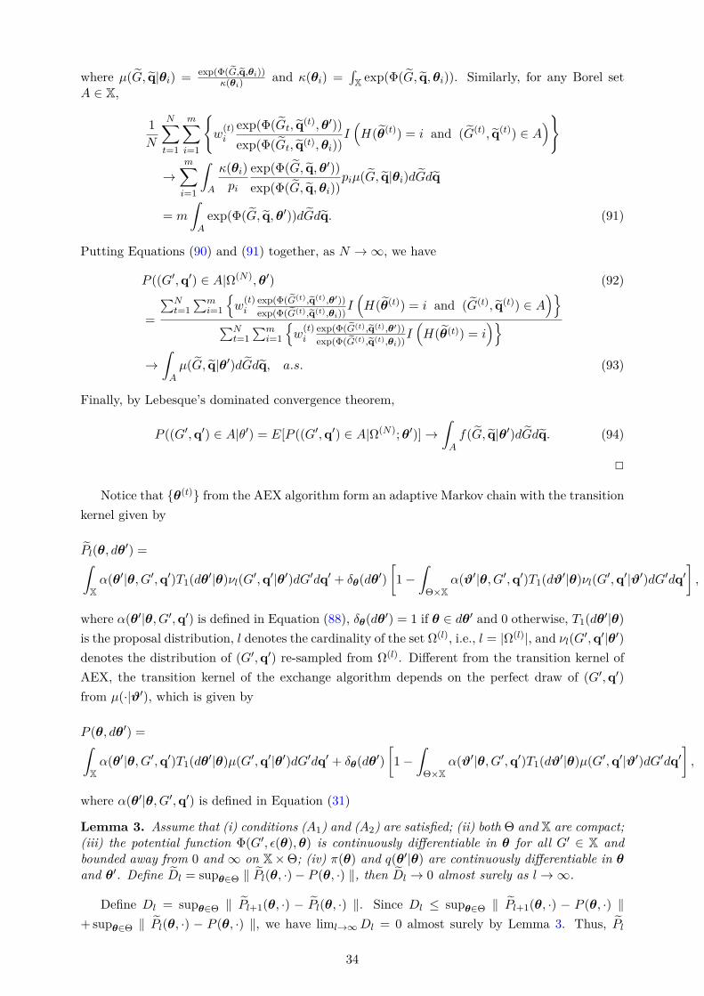
where µ(G, q|θi) = exp(Φ(G,q,θi))κ(θi)
and κ(θi) =∫X exp(Φ(G, q,θi)). Similarly, for any Borel set
A ∈ X,
1
N
N∑t=1
m∑i=1
w
(t)i
exp(Φ(Gt, q(t),θ′))
exp(Φ(Gt, q(t),θi))I(H(θ(t)) = i and (G(t), q(t)) ∈ A
)
→m∑i=1
∫A
κ(θi)
pi
exp(Φ(G, q,θ′))
exp(Φ(G, q,θi))piµ(G, q|θi)dGdq
= m
∫Aexp(Φ(G, q,θ′))dGdq. (91)
Putting Equations (90) and (91) together, as N → ∞, we have
P ((G′,q′) ∈ A|Ω(N),θ′) (92)
=
∑Nt=1
∑mi=1
w
(t)i
exp(Φ(G(t),q(t),θ′))
exp(Φ(G(t),q(t),θi))I(H(θ(t)) = i and (G(t), q(t)) ∈ A
)∑N
t=1
∑mi=1
w
(t)i
exp(Φ(G(t),q(t),θ′))
exp(Φ(G(t),q(t),θi))I(H(θ(t)) = i
)→∫Aµ(G, q|θ′)dGdq, a.s. (93)
Finally, by Lebesque’s dominated convergence theorem,
P ((G′,q′) ∈ A|θ′) = E[P ((G′,q′) ∈ A|Ω(N);θ′)] →∫Af(G, q|θ′)dGdq. (94)
2
Notice that θ(t) from the AEX algorithm form an adaptive Markov chain with the transitionkernel given by
Pl(θ, dθ′) =∫
Xα(θ′|θ, G′,q′)T1(dθ
′|θ)νl(G′,q′|θ′)dG′dq′ + δθ(dθ′)
[1−
∫Θ×X
α(ϑ′|θ, G′,q′)T1(dϑ′|θ)νl(G′,q′|ϑ′)dG′dq′
],
where α(θ′|θ, G′,q′) is defined in Equation (88), δθ(dθ′) = 1 if θ ∈ dθ′ and 0 otherwise, T1(dθ′|θ)is the proposal distribution, l denotes the cardinality of the set Ω(l), i.e., l = |Ω(l)|, and νl(G′,q′|θ′)
denotes the distribution of (G′,q′) re-sampled from Ω(l). Different from the transition kernel ofAEX, the transition kernel of the exchange algorithm depends on the perfect draw of (G′,q′)
from µ(·|ϑ′), which is given by
P (θ, dθ′) =∫Xα(θ′|θ, G′,q′)T1(dθ
′|θ)µ(G′,q′|θ′)dG′dq′ + δθ(dθ′)
[1−
∫Θ×X
α(ϑ′|θ, G′,q′)T1(dϑ′|θ)µ(G′,q′|ϑ′)dG′dq′
],
where α(θ′|θ, G′,q′) is defined in Equation (31)
Lemma 3. Assume that (i) conditions (A1) and (A2) are satisfied; (ii) both Θ and X are compact;(iii) the potential function Φ(G′, ϵ(θ),θ) is continuously differentiable in θ for all G′ ∈ X andbounded away from 0 and ∞ on X×Θ; (iv) π(θ) and q(θ′|θ) are continuously differentiable in θand θ′. Define Dl = supθ∈Θ ∥ Pl(θ, ·)− P (θ, ·) ∥, then Dl → 0 almost surely as l → ∞.
Define Dl = supθ∈Θ ∥ Pl+1(θ, ·) − Pl(θ, ·) ∥. Since Dl ≤ supθ∈Θ ∥ Pl+1(θ, ·) − P (θ, ·) ∥+supθ∈Θ ∥ Pl(θ, ·) − P (θ, ·) ∥, we have liml→∞Dl = 0 almost surely by Lemma 3. Thus, Pl
34
satisfies condition (c) of Theorem D1. It is known that the transition kernel of the exchange algo-rithm, P (θ, dθ′), is irreducible and aperiodic and admits an invariant limit distribution. Lemma4 shows that the transition kernel of the AEX algorithm, Pl(θ, dθ′), also has these properties andthus satisfies condition (a) of Theorem 2.
Lemma 4. Assume (i) the conditions of Lemma 3 are satisfied; (ii) P is irreducible and aperiodicand admits an invariant distribution, then Pl is irreducible and aperiodic, and hence exists astationary distribution πl(θ|G′,q′) such that for any θ0 ∈ Θ,
limk→∞
∥ P kl (θ0, ·)− πl(·|G′,q′) ∥= 0.
Lemma 5 establishes the asymptotic simultaneous uniform ergodicity of the kernel Pl’s.
Lemma 5. Assume the conditions of Lemma 4 are satisfied. If the proposal q(·, ·) satisfies thelocal positive condition, then for any e > 0, there exist a measurable set E(e) in the probabilityspace such that P (E(e)) > 1 − e and on this set E(e), for any ϵ > 0, there exist n(ϵ) ∈ N andl(ϵ) ∈ N such that for any n > n(ϵ) and l > l(ϵ),
∥ Pnl (θ0, ·)− π(·|G,q) ∥≤ ϵ, for all θ0 ∈ Θ.
Putting Lemmas 3, 4, and 5 altogether, we have the following theorem in regard to ergodicityand the weak law of large number for AEX.
Theorem 4. Assume the conditions of Lemma 5 hold. If the proposal T1(·, ·) satisfies the lo-cal positive condition and the unnormalized density function exp(Φ(G′,q′,θ)) is upper semi-continuous in θ for all (G′,q′) ∈ X, then the adaptive exchange algorithm is ergodic and for anybounded measurable function f ,
1
T
T∑t=1
f(θ(t)) → π(f |G,q), in probability,
as T → ∞, where π(f |G,q) =∫Θ f(θ)π(θ|G,q)dθ.
35
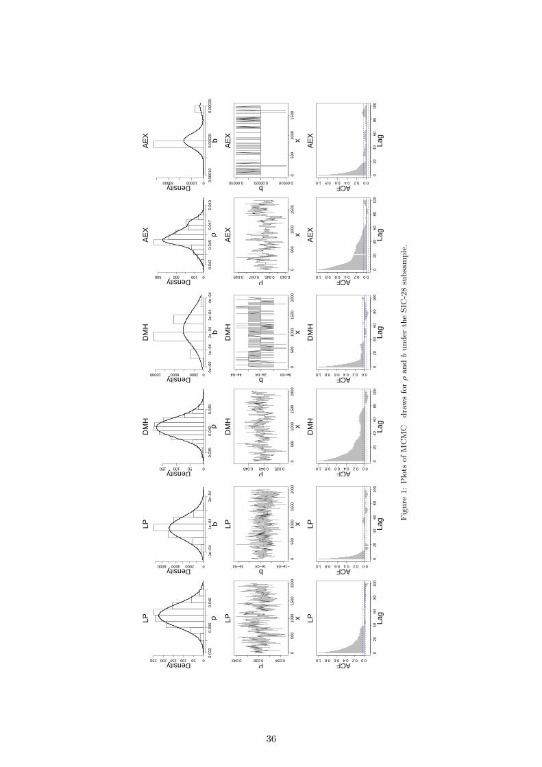
0.03
20.
036
0.04
0
050100150200250
ρ
Density
LP
−1e
−04
1e−
043e
−04
0200040006000
b
Density
LP
050
010
0015
0020
00
0.0340.0380.042
x
ρ
LP
050
010
0015
0020
00
−1e−041e−043e−04
x
b
LP
020
4060
8010
0
0.00.20.40.60.81.0
Lag
ACF
LP
020
4060
8010
0
0.00.20.40.60.81.0
Lag
ACF
LP
0.03
50.
040
0.04
5
050100150
ρ
Density
DM
H
0e+
001e
−04
2e−
043e
−04
4e−
04
02000600010000
b
Density
DM
H
050
010
0015
0020
000.0350.0400.045
xρ
DM
H
050
010
0015
0020
00
0e+002e−044e−04
x
b
DM
H
020
4060
8010
0
0.00.20.40.60.81.0
Lag
ACF
DM
H
020
4060
8010
0
0.00.20.40.60.81.0
Lag
ACF
DM
H
0.04
30.
045
0.04
70.
049
0100300500
ρ
Density
AE
X
0.00
010
0.00
020
0.00
030
01000030000
b
Density
AE
X
050
010
0015
00
0.0430.0450.0470.049
x
ρ
AE
X
050
010
0015
00
0.000100.000200.00030
x
b
AE
X
020
4060
8010
0
0.00.20.40.60.81.0
Lag
ACF
AE
X
020
4060
8010
0
0.00.20.40.60.81.0
Lag
ACF
AE
X
Figu
re1:
Plot
sof
MC
MC
dra
ws
forρ
andb
unde
rth
eSI
C-2
8su
bsam
ple.
36
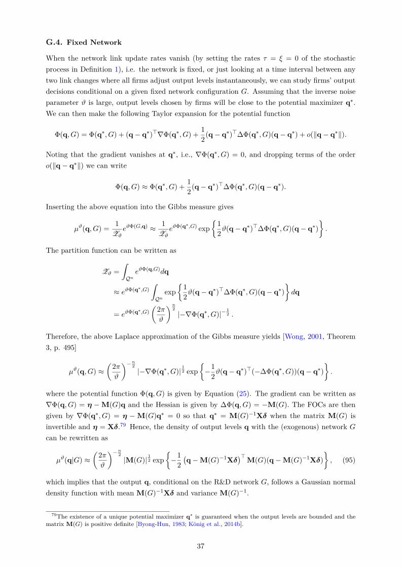
G.4. Fixed Network
When the network link update rates vanish (by setting the rates τ = ξ = 0 of the stochasticprocess in Definition 1), i.e. the network is fixed, or just looking at a time interval between anytwo link changes where all firms adjust output levels instantaneously, we can study firms’ outputdecisions conditional on a given fixed network configuration G. Assuming that the inverse noiseparameter ϑ is large, output levels chosen by firms will be close to the potential maximizer q∗.We can then make the following Taylor expansion for the potential function
Φ(q, G) = Φ(q∗, G) + (q− q∗)⊤∇Φ(q∗, G) +1
2(q− q∗)⊤∆Φ(q∗, G)(q− q∗) + o(∥q− q∗∥).
Noting that the gradient vanishes at q∗, i.e., ∇Φ(q∗, G) = 0, and dropping terms of the ordero(∥q− q∗∥) we can write
Φ(q, G) ≈ Φ(q∗, G) +1
2(q− q∗)⊤∆Φ(q∗, G)(q− q∗).
Inserting the above equation into the Gibbs measure gives
µϑ(q, G) =1
ZϑeϑΦ(G,q) ≈ 1
ZϑeϑΦ(q∗,G) exp
1
2ϑ(q− q∗)⊤∆Φ(q∗, G)(q− q∗)
.
The partition function can be written as
Zϑ =
∫Qn
eϑΦ(q,G)dq
≈ eϑΦ(q∗,G)
∫Qn
exp
1
2ϑ(q− q∗)⊤∆Φ(q∗, G)(q− q∗)
dq
= eϑΦ(q∗,G)
(2π
ϑ
)n2
|−∇Φ(q∗, G)|−12 .
Therefore, the above Laplace approximation of the Gibbs measure yields [Wong, 2001, Theorem3, p. 495]
µϑ(q, G) ≈(2π
ϑ
)−n2
|−∇Φ(q∗, G)|12 exp
−1
2ϑ(q− q∗)⊤(−∆Φ(q∗, G))(q− q∗)
.
where the potential function Φ(q, G) is given by Equation (25). The gradient can be written as∇Φ(q, G) = η −M(G)q and the Hessian is given by ∆Φ(q, G) = −M(G). The FOCs are thengiven by ∇Φ(q∗, G) = η − M(G)q∗ = 0 so that q∗ = M(G)−1Xδ when the matrix M(G) isinvertible and η = Xδ.79 Hence, the density of output levels q with the (exogenous) network Gcan be rewritten as
µϑ(q|G) ≈(2π
ϑ
)−n2
|M(G)|12 exp
−1
2
(q−M(G)−1Xδ
)⊤M(G)(q−M(G)−1Xδ)
, (95)
which implies that the output q, conditional on the R&D network G, follows a Gaussian normaldensity function with mean M(G)−1Xδ and variance M(G)−1.
79The existence of a unique potential maximizer q∗ is guaranteed when the output levels are bounded and thematrix M(G) is positive definite [Byong-Hun, 1983; König et al., 2014b].
37

G.5. Matrix Perturbation
For the computational implementation of the MCMC algorithm we will have to evaluate theinverse of M(G) whenever a link has been added or removed in the network G. To do this in anefficient way, the following lemma will be helpful.
Lemma 6. Let ei and ej be the i-th and j-th unit basis vectors in Rn. The matrix eie⊤j has a
one in the ij-th position and zeros everywhere else. Define the matrix
Bij ≡A−1eie
⊤j A
−1
1 + αe⊤j A−1ei
.
Adding a perturbation α to the matrix A in the ij-th and the ji-th position can be written asA+ αeie
⊤j + ρeje
⊤i .
(i) The inverse of the perturbed matrix can be written as
(A+ αeie⊤j + αeje
⊤i )
−1 = A−1 − αBij − α
(A−1 − αBij
)eje
⊤i
(A−1 − αBij
)1 + αe⊤i (A−1 − αBij) ej
. (96)
(ii) The determinant of the perturbed matrix can be written as
det(A+ αeie⊤j + αeje
⊤i ) =
(1 + αe⊤i
(A−1 − αBij
)ej
)(1 + αe⊤j A
−1ei
)det (A) . (97)
Proof of Lemma 6. We first give a proof of part (i) of the lemma. The Sherman–Morrisonformula states that [Meyer, 2000, page 124]
(A+ αuv⊤)−1 = A−1 − αA−1uv⊤A−1
1 + αv⊤A−1u.
Let c = ei and d = ej , where ei and ej are the i-th and j-th unit basis vectors, respectively.The matrix cd⊤ then has a one in the (i, j)-position and zeros elsewhere, so that adding a one tothe matrix A in the (i, j)-position and the (j, i)-position (resulting from adding a link ij to theadjacency matrix A) yields a perturbed matrix B which can be written as
B = A+ αeie⊤j + αeje
⊤i = C+ αeje
⊤i ,
where we have denoted by C ≡ A + αeie⊤j . Using the Sherman–Morrison formula we then can
write
B−1 = (C+ αeje⊤i )
−1 = C−1 − αC−1eje
⊤i C
−1
1 + αe⊤i C−1ej
, (98)
while applying Sherman–Morrison to C−1 gives
C−1 = (A+ αeie⊤j )
−1 = A−1 − αA−1eie
⊤j A
−1
1 + αe⊤j A−1ei
.
Inserting C−1 into Equation (98) yields
B−1 = A−1 − αA−1eie
⊤j A
−1
1 + αe⊤j A−1ei
− α
(A−1 − α
A−1eie⊤j A−1
1+αe⊤j A−1ei
)eje
⊤i
(A−1 − α
A−1eie⊤j A−1
1+αe⊤j A−1ei
)1 + αe⊤i
(A−1 − α
A−1eie⊤j A−1
1+αe⊤j A−1ei
)ej
.
38
We next give a proof of part (ii) of the lemma. We have that det(A + αeie⊤j + αeje
⊤i ) =
det(C + αeje⊤i ), where we have denoted by C ≡ A + αeie
⊤j . The matrix determinant lemma
states that [Horn and Johnson, 1990]
det(A+ uv⊤) = (1 + v⊤A−1u) det(A).
It then follows that
det(A+ αeie⊤j + αeje
⊤i ) = det(C+ αeje
⊤i ) = (1 + αe⊤i C
−1ej) det (C) ,
Similarly, from the matrix determinant lemma, we have that
det (C) = det(A+ αeie
⊤j
)= (1 + αe⊤j A
−1ei) det (A) .
Further, the Sherman–Morrison formula states that [Meyer, 2000, page 124]
(A+ αcd⊤)−1 = A−1 − αA−1uv⊤A−1
1 + αv⊤A−1u.
It follows that
C−1 = (A+ αeie⊤j )
−1 = A−1 − αA−1eie
⊤j A
−1
1 + αe⊤j A−1ei
.
Putting the above results together, we find that
det(A+ αeie⊤j + αeje
⊤i ) = (1 + αe⊤i C
−1ej) det (C)
=
(1 + αe⊤i
(A−1 − α
A−1eie⊤j A
−1
1 + αe⊤j A−1ei
)ej
)(1 + αe⊤j A
−1ei
)det (A) .
2
Note that due to Lemma 6 the determinant and the inverse of the perturbed matrix A +
αeie⊤j + αeje
⊤i can be efficiently computed if the determinant, det (A), and the inverse, A−1, of
A are already known.
H. Performance of Estimation Methods: Consistency, computation time and miss-ing data
In this paper we consider three types of Bayesian MCMC estimation methods, the likelihood par-tition (LP), the double Metropolis-Hastings (DMH), and the adaptive exchange (AEX) algorithmto estimate our model. In order to demonstrate the performance of each method, we conducta small-scale simulation study to show that (i) the true parameter values can be obtained fromeach method when estimating the correct model, and (ii) to illustrate the relative computationcost of each method. For the first part, as known from the Bayesian identification literature [see,e.g., Berger, 1985, p.224], the Bayesian asymptotic theory related to the posterior distributionis identical to the asymptotic distribution theory for the maximum likelihood estimator (MLE).Therefore, the posterior distribution of parameters should be concentrated at the true value, i.e.,consistent when the sample size goes to infinity (where the role of the prior vanishes), just likeMLE does. Regarding the latter, since estimating ERGMs is usually computationally costly, wereport the computation time (under our simulation design) so that potential users can bettergauge the feasibility of our methods when applied to their own data.
39
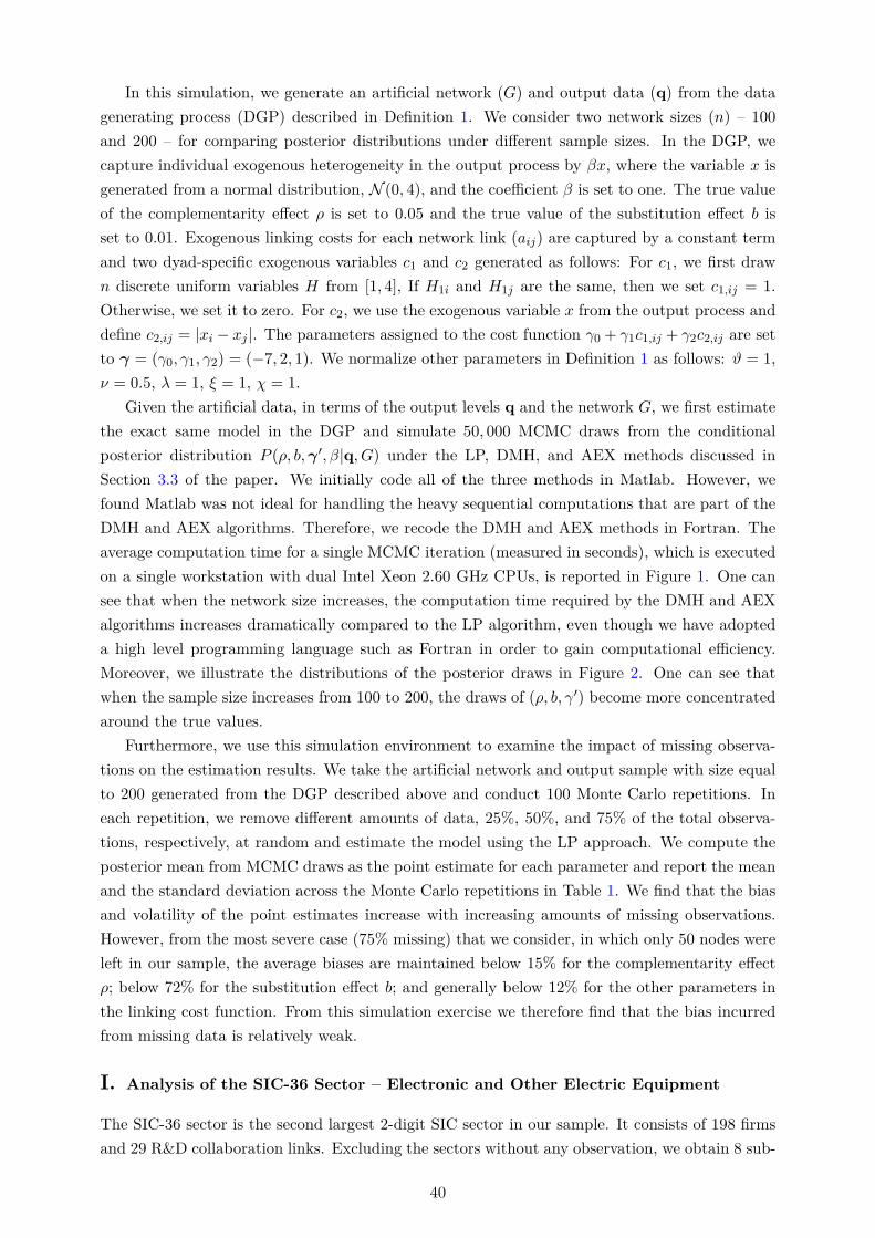
In this simulation, we generate an artificial network (G) and output data (q) from the datagenerating process (DGP) described in Definition 1. We consider two network sizes (n) – 100and 200 – for comparing posterior distributions under different sample sizes. In the DGP, wecapture individual exogenous heterogeneity in the output process by βx, where the variable x isgenerated from a normal distribution, N (0, 4), and the coefficient β is set to one. The true valueof the complementarity effect ρ is set to 0.05 and the true value of the substitution effect b isset to 0.01. Exogenous linking costs for each network link (aij) are captured by a constant termand two dyad-specific exogenous variables c1 and c2 generated as follows: For c1, we first drawn discrete uniform variables H from [1, 4], If H1i and H1j are the same, then we set c1,ij = 1.Otherwise, we set it to zero. For c2, we use the exogenous variable x from the output process anddefine c2,ij = |xi − xj |. The parameters assigned to the cost function γ0 + γ1c1,ij + γ2c2,ij are setto γ = (γ0, γ1, γ2) = (−7, 2, 1). We normalize other parameters in Definition 1 as follows: ϑ = 1,ν = 0.5, λ = 1, ξ = 1, χ = 1.
Given the artificial data, in terms of the output levels q and the network G, we first estimatethe exact same model in the DGP and simulate 50, 000 MCMC draws from the conditionalposterior distribution P (ρ, b,γ ′, β|q, G) under the LP, DMH, and AEX methods discussed inSection 3.3 of the paper. We initially code all of the three methods in Matlab. However, wefound Matlab was not ideal for handling the heavy sequential computations that are part of theDMH and AEX algorithms. Therefore, we recode the DMH and AEX methods in Fortran. Theaverage computation time for a single MCMC iteration (measured in seconds), which is executedon a single workstation with dual Intel Xeon 2.60 GHz CPUs, is reported in Figure 1. One cansee that when the network size increases, the computation time required by the DMH and AEXalgorithms increases dramatically compared to the LP algorithm, even though we have adopteda high level programming language such as Fortran in order to gain computational efficiency.Moreover, we illustrate the distributions of the posterior draws in Figure 2. One can see thatwhen the sample size increases from 100 to 200, the draws of (ρ, b, γ′) become more concentratedaround the true values.
Furthermore, we use this simulation environment to examine the impact of missing observa-tions on the estimation results. We take the artificial network and output sample with size equalto 200 generated from the DGP described above and conduct 100 Monte Carlo repetitions. Ineach repetition, we remove different amounts of data, 25%, 50%, and 75% of the total observa-tions, respectively, at random and estimate the model using the LP approach. We compute theposterior mean from MCMC draws as the point estimate for each parameter and report the meanand the standard deviation across the Monte Carlo repetitions in Table 1. We find that the biasand volatility of the point estimates increase with increasing amounts of missing observations.However, from the most severe case (75% missing) that we consider, in which only 50 nodes wereleft in our sample, the average biases are maintained below 15% for the complementarity effectρ; below 72% for the substitution effect b; and generally below 12% for the other parameters inthe linking cost function. From this simulation exercise we therefore find that the bias incurredfrom missing data is relatively weak.
I. Analysis of the SIC-36 Sector – Electronic and Other Electric Equipment
The SIC-36 sector is the second largest 2-digit SIC sector in our sample. It consists of 198 firmsand 29 R&D collaboration links. Excluding the sectors without any observation, we obtain 8 sub-
40
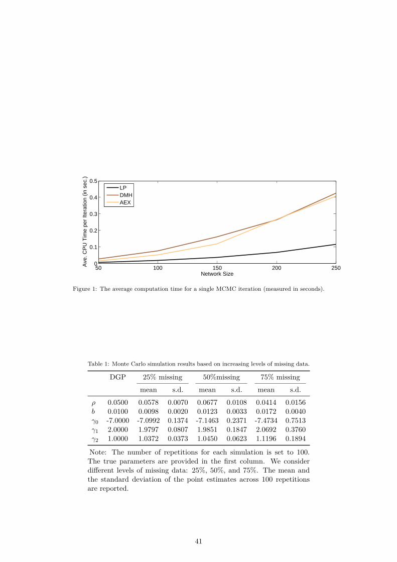
50 100 150 200 2500
0.1
0.2
0.3
0.4
0.5
Network Size
Ave
. CP
U T
ime
per
Itera
tion
(in s
ec.)
LPDMHAEX
Figure 1: The average computation time for a single MCMC iteration (measured in seconds).
Table 1: Monte Carlo simulation results based on increasing levels of missing data.
DGP 25% missing 50%missing 75% missingmean s.d. mean s.d. mean s.d.
ρ 0.0500 0.0578 0.0070 0.0677 0.0108 0.0414 0.0156b 0.0100 0.0098 0.0020 0.0123 0.0033 0.0172 0.0040γ0 -7.0000 -7.0992 0.1374 -7.1463 0.2371 -7.4734 0.7513γ1 2.0000 1.9797 0.0807 1.9851 0.1847 2.0692 0.3760γ2 1.0000 1.0372 0.0373 1.0450 0.0623 1.1196 0.1894
Note: The number of repetitions for each simulation is set to 100.The true parameters are provided in the first column. We considerdifferent levels of missing data: 25%, 50%, and 75%. The mean andthe standard deviation of the point estimates across 100 repetitionsare reported.
41
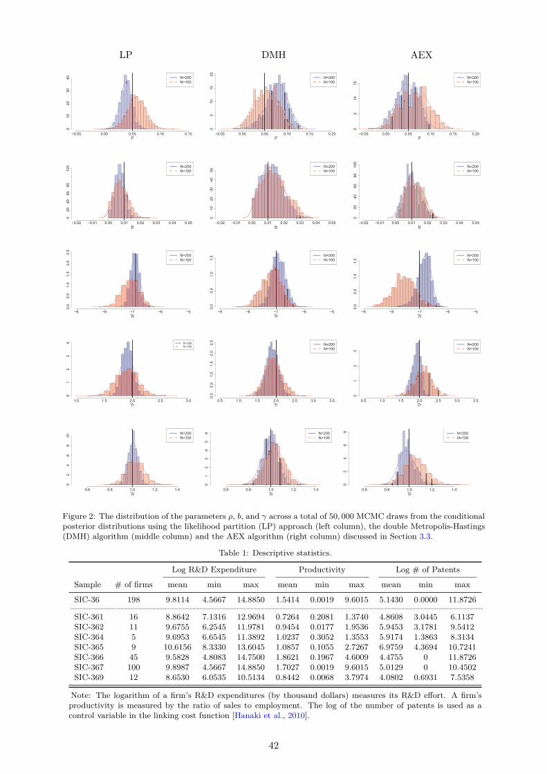
LP DMH AEX
ρ−0.05 0.00 0.05 0.10 0.15
010
20
30
40 N=200
N=100
ρ−0.05 0.00 0.05 0.10 0.15 0.20
05
10
15
20
N=200
N=100
ρ−0.05 0.00 0.05 0.10 0.15 0.20
05
10
15
N=200
N=100
b
−0.02 −0.01 0.00 0.01 0.02 0.03 0.04 0.05
020
40
60
80
120 N=200
N=100
b
−0.02 −0.01 0.00 0.01 0.02 0.03 0.04 0.05
010
20
30
40
50
N=200
N=100
b
−0.02 −0.01 0.00 0.01 0.02 0.03 0.04 0.05
020
40
60
80
100
N=200
N=100
γ0−9 −8 −7 −6 −5
0.0
0.5
1.0
1.5
2.0
2.5
N=200
N=100
γ0−9 −8 −7 −6 −5
0.0
0.5
1.0
1.5
N=200
N=100
γ0−9 −8 −7 −6 −5
0.0
0.5
1.0
1.5
N=200
N=100
γ11.0 1.5 2.0 2.5 3.0
01
23
4 N=200
N=100
γ10.5 1.0 1.5 2.0 2.5 3.0 3.5
0.0
0.5
1.0
1.5
2.0
2.5
N=200
N=100
γ10.5 1.0 1.5 2.0 2.5 3.0 3.5
01
23
N=200
N=100
γ20.6 0.8 1.0 1.2 1.4
02
46
810 N=200
N=100
γ20.6 0.8 1.0 1.2 1.4
01
23
45
6 N=200
N=100
γ20.6 0.8 1.0 1.2 1.4
02
46
8
N=200
N=100
Figure 2: The distribution of the parameters ρ, b, and γ across a total of 50, 000 MCMC draws from the conditionalposterior distributions using the likelihood partition (LP) approach (left column), the double Metropolis-Hastings(DMH) algorithm (middle column) and the AEX algorithm (right column) discussed in Section 3.3.
Table 1: Descriptive statistics.
Log R&D Expenditure Productivity Log # of Patents
Sample # of firms mean min max mean min max mean min max
SIC-36 198 9.8114 4.5667 14.8850 1.5414 0.0019 9.6015 5.1430 0.0000 11.8726
SIC-361 16 8.8642 7.1316 12.9694 0.7264 0.2081 1.3740 4.8608 3.0445 6.1137SIC-362 11 9.6755 6.2545 11.9781 0.9454 0.0177 1.9536 5.9453 3.1781 9.5412SIC-364 5 9.6953 6.6545 11.3892 1.0237 0.3052 1.3553 5.9174 1.3863 8.3134SIC-365 9 10.6156 8.3330 13.6045 1.0857 0.1055 2.7267 6.9759 4.3694 10.7241SIC-366 45 9.5828 4.8083 14.7500 1.8621 0.1967 4.6009 4.4755 0 11.8726SIC-367 100 9.8987 4.5667 14.8850 1.7027 0.0019 9.6015 5.0129 0 10.4502SIC-369 12 8.6530 6.0535 10.5134 0.8442 0.0068 3.7974 4.0802 0.6931 7.5358
Note: The logarithm of a firm’s R&D expenditures (by thousand dollars) measures its R&D effort. A firm’sproductivity is measured by the ratio of sales to employment. The log of the number of patents is used as acontrol variable in the linking cost function [Hanaki et al., 2010].
42
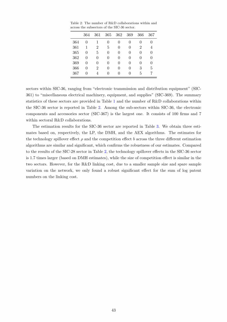
Table 2: The number of R&D collaborations within andacross the subsectors of the SIC-36 sector.
364 361 365 362 369 366 367364 0 1 0 0 0 0 0361 1 2 5 0 0 2 4365 0 5 0 0 0 0 0362 0 0 0 0 0 0 0369 0 0 0 0 0 0 0366 0 2 0 0 0 3 5367 0 4 0 0 0 5 7
sectors within SIC-36, ranging from “electronic transmission and distribution equipment” (SIC-361) to “miscellaneous electrical machinery, equipment, and supplies” (SIC-369). The summarystatistics of these sectors are provided in Table 1 and the number of R&D collaborations withinthe SIC-36 sector is reported in Table 2. Among the sub-sectors within SIC-36, the electroniccomponents and accessories sector (SIC-367) is the largest one. It consists of 100 firms and 7within sectoral R&D collaborations.
The estimation results for the SIC-36 sector are reported in Table 3. We obtain three esti-mates based on, respectively, the LP, the DMH, and the AEX algorithms. The estimates forthe technology spillover effect ρ and the competition effect b across the three different estimationalgorithms are similar and significant, which confirms the robustness of our estimates. Comparedto the results of the SIC-28 sector in Table 2, the technology spillover effects in the SIC-36 sectoris 1.7 times larger (based on DMH estimates), while the size of competition effect is similar in thetwo sectors. However, for the R&D linking cost, due to a smaller sample size and spare samplevariation on the network, we only found a robust significant effect for the sum of log patentnumbers on the linking cost.
43
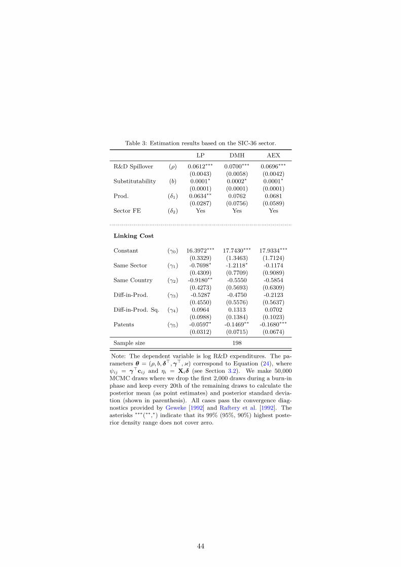
Table 3: Estimation results based on the SIC-36 sector.
LP DMH AEX
R&D Spillover (ρ) 0.0612∗∗∗ 0.0700∗∗∗ 0.0696∗∗∗
(0.0043) (0.0058) (0.0042)Substitutability (b) 0.0001∗ 0.0002∗ 0.0001∗
(0.0001) (0.0001) (0.0001)Prod. (δ1) 0.0634∗∗ 0.0762 0.0681
(0.0287) (0.0756) (0.0589)Sector FE (δ2) Yes Yes Yes
Linking Cost
Constant (γ0) 16.3972∗∗∗ 17.7430∗∗∗ 17.9334∗∗∗
(0.3329) (1.3463) (1.7124)Same Sector (γ1) -0.7698∗ -1.2118∗ -0.1174
(0.4309) (0.7709) (0.9089)Same Country (γ2) -0.9180∗∗ -0.5550 -0.5854
(0.4273) (0.5693) (0.6309)Diff-in-Prod. (γ3) -0.5287 -0.4750 -0.2123
(0.4550) (0.5576) (0.5637)Diff-in-Prod. Sq. (γ4) 0.0964 0.1313 0.0702
(0.0988) (0.1384) (0.1023)Patents (γ5) -0.0597∗ -0.1469∗∗ -0.1680∗∗∗
(0.0312) (0.0715) (0.0674)
Sample size 198
Note: The dependent variable is log R&D expenditures. The pa-rameters θ = (ρ, b, δ⊤,γ⊤,κ) correspond to Equation (24), whereψij = γ⊤cij and ηi = Xiδ (see Section 3.2). We make 50,000MCMC draws where we drop the first 2,000 draws during a burn-inphase and keep every 20th of the remaining draws to calculate theposterior mean (as point estimates) and posterior standard devia-tion (shown in parenthesis). All cases pass the convergence diag-nostics provided by Geweke [1992] and Raftery et al. [1992]. Theasterisks ∗∗∗(∗∗,∗) indicate that its 99% (95%, 90%) highest poste-rior density range does not cover zero.
44
ReferencesAhuja, G. (2000). Collaboration networks, structural holes, and innovation: A longitudinal study. Administrative
Science Quarterly, 45(3):425–455.Anderson, S., Goeree, J., and Holt, C. (2004). Noisy directional learning and the logit equilibrium. Scandinavian
Journal of Economics, 106(3):581–602.Anderson, S. P., De Palma, A., and Thisse, J. F. (1992). Discrete choice theory of product differentiation. MIT
Press.Anderson, S. P., Goeree, J. K., and Holt, C. A. (2001). Minimum-effort coordination games: Stochastic potential
and logit equilibrium. Games and Economic Behavior, 34(2):177–199.Atkinson, K. E. (1989). An introduction to numerical analysis. John Wiley & Sons.Ballester, C., Calvó-Armengol, A., and Zenou, Y. (2006). Who’s who in networks. wanted: The key player.
Econometrica, 74(5):1403–1417.Banerjee, A. and Duflo, E. (2005). Growth theory through the lens of development economics. Handbook of
Economic growth, 1:473–552.Baum, J., Cowan, R., and Jonard, N. (2009). Network-independent partner selection and the evolution of innovation
networks. UNU-MERIT working paper series; 2009-022.Belderbos, R., Carree, M., and Lokshin, B. (2004). Cooperative r&d and firm performance. Research policy,
33(10):1477–1492.Ben-Akiva, M. and Watanatada, T. (1981). Application of a continuous spatial choice logit model. Structural
analysis of discrete data with econometric applications, pages 320–343.Bena, J., Fons-Rosen, C., and Ondko, P. (2008). Zephyr: Ownership changes database. London School of Economics
working paper.Berger, J. O. (1985). Statistical Decision Theory and Bayesian Analysis. Springer Science & Business Media.Berliant, M. and Fujita, M. (2008). Knowledge creation as a square dance on the hilbert cube. International
Economic Review, 49(4):1251–1295.Berliant, M. and Fujita, M. (2009). Dynamics of knowledge creation and transfer: The two person case. Interna-
tional Journal of Economic Theory, 5(2):155–179.Bernstein, J. I. (1988). Costs of production, intra-and interindustry R&D spillovers: Canadian evidence. Canadian
Journal of Economics, 21(2):324–347.Bloom, N., Schankerman, M., and Van Reenen, J. (2013). Identifying technology spillovers and product market
rivalry. Econometrica, 81(4):1347–1393.Blundell, R., Griffith, R., and Van Reenen, J. (1995). Dynamic count data models of technological innovation. The
Economic Journal, 105(429):333–344.Bollaert, H. and Delanghe, M. (2015). Securities data company and zephyr, data sources for m&a research. Journal
of Corporate Finance.Bollobás, B., Janson, S., and Riordan, O. (2007). The phase transition in inhomogeneous random graphs. Random
Structures & Algorithms, 31(1):3–122.Brualdi, R. A. and Solheid, Ernie, S. (1986). On the spectral radius of connected graphs. Publications de l’ Institute
Mathématique, 53:45–54.Byong-Hun, A. (1983). Iterative methods for linear complementarity problems with upper bounds on primary
variables. Mathematical Programming, 26(3):295–315.Chatterjee, S., Diaconis, P., and Sly, A. (2011). Random graphs with a given degree sequence. The Annals of
Applied Probability, 21(4):1400–1435.Chib, S. and Greenberg, E. (1996). Markov chain Monte Carlo simulation methods in econometrics. Econometric
theory, 12(03):409–431.Cohen, W. and Klepper, S. (1996a). Firm size and the nature of innovation within industries: the case of process
and product R&D. The Review of Economics and Statistics, 78(2):232–243.Cohen, W. and Klepper, S. (1996b). A reprise of size and R&D. The Economic Journal, 106(437):925–951.Copeland, A. and Fixler, D. (2012). Measuring the price of research and development output. Review of Income
and Wealth, 58(1):166–182.Cvetkovic, D. and Rowlinson, P. (1990). The largest eigenvalue of a graph: A survey. Linear and Multinilear
Algebra, 28(1):3–33.Dai, R. (2012). International accounting databases on WRDS: Comparative analysis. Working paper, Wharton
Research Data Services, University of Pennsylvania.D’Aspremont, C. and Jacquemin, A. (1988). Cooperative and noncooperative R&D in duopoly with spillovers. The
American Economic Review, 78(5):1133–1137.Deijfen, M. and Kets, W. (2009). Random intersection graphs with tunable degree distribution and clustering.
Probability in the Engineering and Informational Sciences, 23(04):661–674.Dell, M. (2009). GIS analysis for applied economists. Mimeo, MIT Department of Economics.D’Haultfœuille, X. and Iaria, A. (2016). A convenient method for the estimation of the multinomial logit model
with fixed effects. Economics Letters, 141:77–79.Dorogovtsev, S. N. and Mendes, J. F. (2013). Evolution of networks: From biological nets to the Internet and
WWW. Oxford University Press.Fafchamps, M. and Gubert, F. (2007). The formation of risk sharing networks. Journal of Development Economics,
83(2):326–350.Fort, G., Moulines, E., and Priouret, P. (2011). Convergence of adaptive and interacting Markov chain Monte
Carlo algorithms. The Annals of Statistics, 36(4):3262–3289.Geweke, J. (1992). Evaluating the accuracy of sampling-based approaches to the calculation of posterior moments.
Bayesian Statistics, pages 169–193.Graham, B. S. (2014). An empirical model of network formation: detecting homophily when agents are heteroge-
nous. National Bureau of Economic Research Working Paper No. w20341.Graham, B. S. (2015). Methods of identification in social networks. Annual Review of Economics, 7(1):465–485.Griffith, R., Redding, S., and Van Reenen, J. (2003). R&D and absorptive capacity: Theory and empirical evidence.
45
Scandinavian Journal of Economics, 105(1):99–118.Hagedoorn, J. (2002). Inter-firm R&D partnerships: an overview of major trends and patterns since 1960. Research
Policy, 31(4):477–492.Hanaki, N., Nakajima, R., and Ogura, Y. (2010). The dynamics of R&D network in the IT industry. Research
Policy, 39(3):386–399.Horn, R. A. and Johnson, C. R. (1990). Matrix Analysis. Cambridge University Press.Huyghebaert, N. and Luypaert, M. (2010). Antecedents of growth through mergers and acquisitions: Empirical
results from belgium. Journal of Business Research, 63(4):392–403.Jaffe, A. and Trajtenberg, M. (2002). Patents, Citations, and Innovations: A Window on the Knowledge Economy.
MIT Press.Jaffe, A. B. (1989). Characterizing the technological position of firms, with application to quantifying technological
opportunity and research spillovers. Research Policy, 18(2):87 – 97.Jin, I. H., Yuan, Y., and Liang, F. (2013). Bayesian analysis for exponential random graph models using the
adaptive exchange sampler. Statistics and its interface, 6(4):559.Kamien, M. I., Muller, E., and Zang, I. (1992). Research joint ventures and R&D cartels. The American Economic
Review, 82(5):1293–1306.König, M., Tessone, C., and Zenou, Y. (2014a). Nestedness in networks: A theoretical model and some applications.
Theoretical Economics, 9:695–752.König, M. D., Liu, X., and Zenou, Y. (2014b). R&D networks: Theory, empirics and policy implications. CEPR
Discussion Paper No. 9872.König, M. D., Lorenz, J., and Zilibotti, F. (2016). Innovation vs. imitation and the evolution of productivity
distributions. Theoretical Economics, 11:1053–1102.Koop, G., Poirier, D. J., and Tobias, J. L. (2007). Bayesian econometric methods. Cambridge University Press.Liang, F., Jin, I. H., Song, Q., and Liu, J. S. (2015). An adaptive exchange algorithm for sampling from distributions
with intractable normalizing constants. Journal of the American Statistical Association, 111(513):377–393.Liben-Nowell, D. and Kleinberg, J. (2007). The link-prediction problem for social networks. Journal of the American
society for information science and technology, 58(7):1019–1031.Lychagin, S., Pinkse, J., Slade, M. E., and Van Reenen, J. (2016). Spillovers in space: does geography matter?
The Journal of Industrial Economics, 64(2):295–335.Mahadev, N. and Peled, U. (1995). Threshold Graphs and Related Topics. North Holland.McFadden, D. (1976). The mathematical theory of demand models. Behavioral Travel Demand Models, pages
305–314.McManus, O., Blatz, A., and Magleby, K. (1987). Sampling, log binning, fitting, and plotting durations of open
and shut intervals from single channels and the effects of noise. Pflügers Archiv, 410(4-5):530–553.Mele, A. (2017). A structural model of dense network formation. Econometrica, 85(3):825–850.Melitz, M. (2003). The impact of trade on intra-industry reallocations and aggregate industry productivity. Econo-
metrica, 71(6):1695–1725.Melitz, M., Ottaviano, G., and Maggiore, S. (2008). Market Size, Trade, and Productivity. Review of Economic
Studies, 75(1):295–316.Meyer, C. D. (2000). Matrix analysis and applied linear algebra. Society for Industrial and Applied Mathematics.Nooteboom, B., Van Haverbeke, W., Duysters, G., Gilsing, V., and Van Den Oord, A. (2007). Optimal cognitive
distance and absorptive capacity. Research Policy, 36(7):1016–1034.Papadopoulos, A. (2012). Sources of data for international business research: Availabilities and implications for
researchers. In Academy of Management Proceedings, volume 2012, pages 1–1. Academy of Management.Peled, U. N., Petreschi, R., and Sterbini, A. (1999). (n, e)-graphs with maximum sum of squares of degrees. Journal
of Graph Theory, 31(4):283–295.Powell, W., Koput, K. W., and Smith-Doerr, L. (1996). Interorganizational collaboration and the locus of innova-
tion: Networks of learning in biotechnology. Administrative Science Quarterly, 41(1):116–145.Powell, W. W., White, D. R., Koput, K. W., and Owen-Smith, J. (2005). Network dynamics and field evolution:
The growth of interorganizational collaboration in the life sciences. American Journal of Sociology, 110(4):1132–1205.
Raftery, A. E., Lewis, S., Banfield, J. D., and Rafterv, A. E. (1992). How many iterations in the Gibbs sampler.Bayesian Statistics, page 4.
Robert, C. and Casella, G. (2004). Monte Carlo statistical methods. Springer Verlag.Roberts, G. O. and Rosenthal, J. S. (2007). Coupling and ergodicity of adaptive Markov chain Monte Carlo
algorithms. Journal of applied probability, 44(2):458–475.Roberts, G. O. and Tweedie, R. L. (1996). Geometric convergence and central limit theorems for multidimensional
Hastings and Metropolis algorithms. Biometrika, 83(1):95–110.Roijakkers, N. and Hagedoorn, J. (2006). Inter-firm R&D partnering in pharmaceutical biotechnology since 1975:
Trends, patterns, and networks. Research Policy, 35(3):431–446.Schilling, M. (2009). Understanding the alliance data. Strategic Management Journal, 30(3):233–260.Singh, N. and Vives, X. (1984). Price and quantity competition in a differentiated duopoly. The RAND Journal
of Economics, 15(4):546–554.Snijders, T. (2002). Markov chain Monte Carlo estimation of exponential random graph models. Journal of Social
Structure, 3(2):1–40.Söderberg, B. (2002). General formalism for inhomogeneous random graphs. Physical Review E, 66(6):066121.Spence, M. (1984). Cost reduction, competition, and industry performance. Econometrica, 52(1):101–122.Thoma, G., Torrisi, S., Gambardella, A., Guellec, D., Hall, B. H., and Harhoff, D. (2010). Harmonizing and
combining large datasets-an application to firm-level patent and accounting data. National Bureau of EconomicResearch Working Paper No. w15851.
Tierney, L. (1994). Markov chains for exploring posterior distributions. the Annals of Statistics, 22(4):1701–1728.Trajtenberg, M., Shiff, G., and Melamed, R. (2009). The “names game”: Harnessing inventors, patent data for
economic research. Annals of Economics and Statistics, (93/94):79–108.Vincenty, T. (1975). Direct and inverse solutions of geodesics on the ellipsoid with application of nested equations.
46

Survey review, 23(176):88–93.Westbrock, B. (2010). Natural concentration in industrial research collaboration. The RAND Journal of Economics,
41(2):351–371.Wong, R. (2001). Asymptotic approximations of integrals, volume 34. Society for Industrial Mathematics.
47