Network Externalities and Market Dominance∗

Robert Akerlof† Richard Holden‡ Luis Rayo§

April 10, 2018

Abstract

We develop a framework to study optimal pricing and price competitionin the presence of multiple equilibria caused by network externalities. Thisframework provides a simple approach to equilibrium selection, based uponconsumers’ “impulses,” that yields concise predictions regarding when firmswill be “in” and when “out.” We highlight the role of past consumption and“influencers” in shaping impulses, and provide a unified explanation for a va-riety of stylized facts including why: (i) it is difficult to become “in”; (ii) the“in” position is fragile; (iii) “in” firms are not asleep in the sense that they con-tinuously raise quality and keep prices low; and (iv) “in” firms acquire startupsto entrench their position.

∗We are grateful to Gonzalo Cisternas, Luis Garicano, Bob Gibbons, Tom Hubbard, BobPindyck, and seminar participants at Kellogg, MIT, Melbourne, and UNSW for helpful discussions.Akerlof acknowledges support from the Institute for New Economic Thinking (INET). Holden ac-knowledges support from the Australian Research Council (ARC) Future Fellowship FT130101159.Rayo acknowledges support from the Marriner S. Eccles Institute for Economics and QuantitativeAnalysis.†University of Warwick and CEPR, r.akerlof@warwick.ac.uk.‡UNSW Australia Business School, richard.holden@unsw.edu.au.§University of Utah and CEPR, luis.rayo@eccles.utah.edu.

1 Introduction

Many markets exhibit significant network externalities. These markets have threekey features. First, winning firms serve a disproportionate share of their markets,with a large size gap between them and their closest rivals. Indeed, the five largestpublicly traded companies in the world (Apple, Google/Alphabet, Microsoft, Ama-zon, Facebook) all operate in such markets.

Second, it is difficult to become a winner and yet success is so fragile that it canvanish overnight. The difficulties of becoming popular (going from being “out” tobeing “in”) are illustrated by Microsoft’s search engine Bing, which despite years ofsizeable investments remains much smaller than the current superstar Google. Theease with which a successful firm can suddenly fail (going from “in” to “out”) isillustrated by the web browser Netscape, which despite its initial dominant statuswas overtaken quite suddenly by Microsoft’s Internet Explorer.

Finally, despite their seemingly dominant position, winners are not asleep. Win-ners tend to continuously raise quality (for example, by purchasing new startups)while at the same time keeping their prices low, sometimes even below average cost.

The pioneering work of Katz and Shapiro (1985) and Becker (1991) shows thatnetwork externalities can generate demand curves with both downward- and upward-sloping regions, depending on whether the traditional price effect or the network effectdominates. Such demand curves admit the possibility of multiple equilibria.

Equilibrium selection — whether firms end up “in” or “out” — is central tounderstanding these markets. It underlies issues of firm strategy, such as optimalpricing and incentives for innovation; the outcome of competition; and appropriateantitrust policy. Our main contribution in this paper is to offer a tractable theoryof equilibrium selection in these markets, based upon Kets and Sandroni (2017)’sconcept of introspective equilibrium. Our refinement emphasizes the economic im-portance of consumers’ “impulses” for equilibrium selection, as well as the roles ofpast consumption and “influencers” in shaping these impulses. As we shall see, thistheory accounts for the three features of markets with network externalities men-tioned above.

1

We are certainly not the first to study markets with network externalities. Ro-chet and Tirole (2003) observed that many of these markets are multi-sided andinvolve interaction through platforms; and they initiated a literature analyzing suchmarkets.1 There is also a literature on “switching costs” beginning with Klemperer(1987) (see also Klemperer (1995) and Farrell and Klemperer (2007)). Like us, thisliterature emphasizes the importance of past consumption for present consumption.Finally, in our model a dominant (“in”) firm is disciplined in the price it charges by“out” firms with lower market share — a feature that bears some similarity to theliterature on “limit pricing.”2

What distinguishes our approach from the above work is our emphasis on equi-librium selection.3

The remainder of the paper is organized as follows. Section 2 presents the baselinemodel with a single firm. Section 3 considers price competition among two firms.Section 4 considers the special case of a piecewise linear demand curve. Section 5extends our model to multi-sided markets, and Section 6 concludes.

2 Monopoly Case

To begin, we will consider a setting with a single firm (a monopolist). We assumethat each period (t = 1, 2, ..., T ) the monopolist chooses a price pt. The marginalcost of production is constant — and we normalize it to zero.

There is a set of heterogeneous consumers. Consumer i’s demand at time t,denoted qti , depends upon the price pt and upon aggregate consumption Qt; that is,qti = Di(pt, Qt). We assume Di is decreasing in pt and increasing in Qt, reflecting thepresence of positive network externalities.

For any given pt, an equilibrium quantity Qt∗ satisfies:1Some notable contributions include Rochet and Tirole (2006), Armstrong (2006), and Weyl

(2010).2For classic references on limit pricing, see Gaskins (1971) and Milgrom and Roberts (1982), and

for a more recent contribution that focuses on entry deterrence in markets with network externalitiessee Fudenberg and Tirole (2000).

3Existing work typically follows the convention that consumers coordinate on the equilibriumwith the highest level of sales (e.g., Fudenberg and Tirole (2000)).

2

Qt∗ =∑i

Di

(pt, Qt∗

).

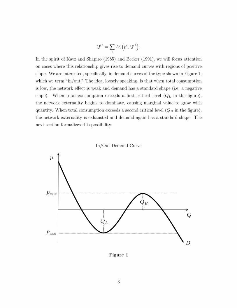
In the spirit of Katz and Shapiro (1985) and Becker (1991), we will focus attentionon cases where this relationship gives rise to demand curves with regions of positiveslope. We are interested, specifically, in demand curves of the type shown in Figure 1,which we term “in/out.” The idea, loosely speaking, is that when total consumptionis low, the network effect is weak and demand has a standard shape (i.e. a negativeslope). When total consumption exceeds a first critical level (QL in the figure),the network externality begins to dominate, causing marginal value to grow withquantity. When total consumption exceeds a second critical level (QH in the figure),the network externality is exhausted and demand again has a standard shape. Thenext section formalizes this possibility.

In/Out Demand Curve“In/Out” Demand Curve

QH

QL

D

Q

pmax

pmin

p

Figure 1

3

2.1 Micro-foundation for In/Out Demand

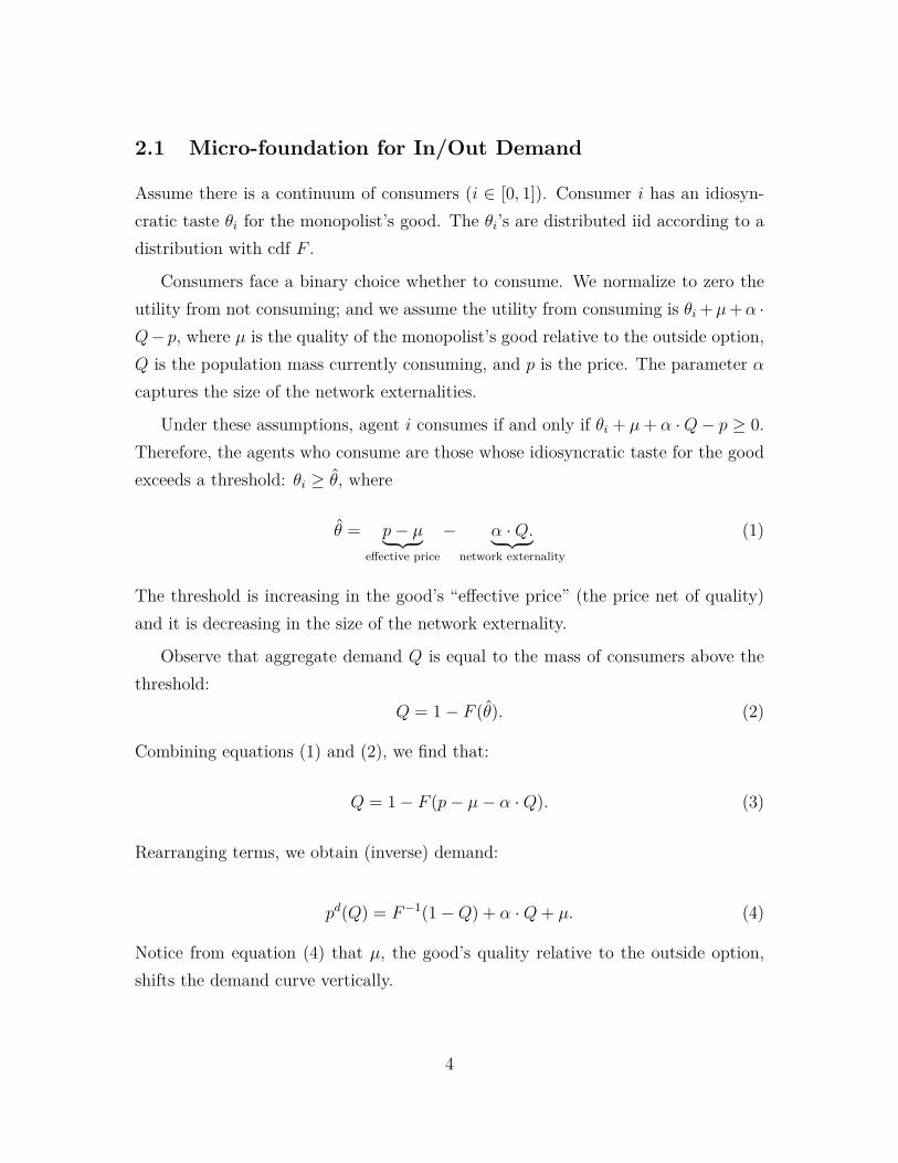
Assume there is a continuum of consumers (i ∈ [0, 1]). Consumer i has an idiosyn-cratic taste θi for the monopolist’s good. The θi’s are distributed iid according to adistribution with cdf F .

Consumers face a binary choice whether to consume. We normalize to zero theutility from not consuming; and we assume the utility from consuming is θi +µ+α ·Q− p, where µ is the quality of the monopolist’s good relative to the outside option,Q is the population mass currently consuming, and p is the price. The parameter αcaptures the size of the network externalities.

Under these assumptions, agent i consumes if and only if θi + µ+ α ·Q− p ≥ 0.Therefore, the agents who consume are those whose idiosyncratic taste for the goodexceeds a threshold: θi ≥ θ̂, where

θ̂ = p− µ︸ ︷︷ ︸effective price

− α ·Q.︸ ︷︷ ︸network externality

(1)

The threshold is increasing in the good’s “effective price” (the price net of quality)and it is decreasing in the size of the network externality.

Observe that aggregate demand Q is equal to the mass of consumers above thethreshold:

Q = 1− F (θ̂). (2)

Combining equations (1) and (2), we find that:

Q = 1− F (p− µ− α ·Q). (3)

Rearranging terms, we obtain (inverse) demand:

pd(Q) = F−1(1−Q) + α ·Q+ µ. (4)

Notice from equation (4) that µ, the good’s quality relative to the outside option,shifts the demand curve vertically.

4

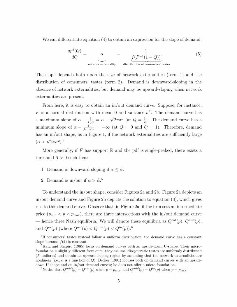
We can differentiate equation (4) to obtain an expression for the slope of demand:

dpd(Q)dQ

= α︸︷︷︸network externality

− 1f(F−1(1−Q)) .︸ ︷︷ ︸

distribution of consumers’ tastes

(5)

The slope depends both upon the size of network externalities (term 1) and thedistribution of consumers’ tastes (term 2). Demand is downward-sloping in theabsence of network externalities; but demand may be upward-sloping when networkexternalities are present.

From here, it is easy to obtain an in/out demand curve. Suppose, for instance,F is a normal distribution with mean 0 and variance σ2. The demand curve hasa maximum slope of α − 1

f(0) = α −√

2πσ2 (at Q = 12). The demand curve has a

minimum slope of α − 1f(±∞) = −∞ (at Q = 0 and Q = 1). Therefore, demand

has an in/out shape, as in Figure 1, if the network externalities are sufficiently large(α >

√2πσ2).4

More generally, if F has support R and the pdf is single-peaked, there exists athreshold α̂ > 0 such that:

1. Demand is downward-sloping if α ≤ α̂.

2. Demand is in/out if α > α̂.5

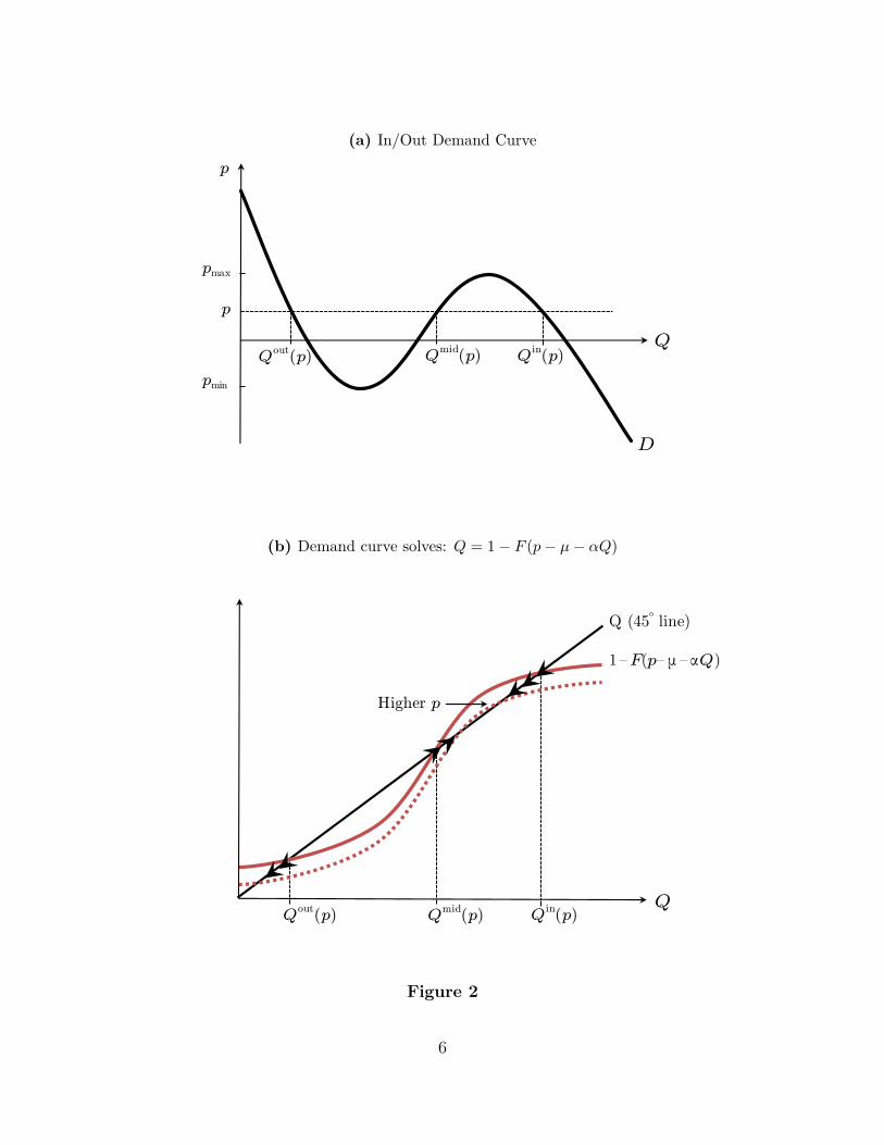
To understand the in/out shape, consider Figures 2a and 2b. Figure 2a depicts anin/out demand curve and Figure 2b depicts the solution to equation (3), which givesrise to this demand curve. Observe that, in Figure 2a, if the firm sets an intermediateprice (pmin < p < pmax), there are three intersections with the in/out demand curve— hence three Nash equilibria. We will denote these equilibria as Qout(p), Qmid(p),and Qin(p) (where Qout(p) < Qmid(p) < Qin(p)).6

4If consumers’ tastes instead follow a uniform distribution, the demand curve has a constantslope because f(θ) is constant.

5Katz and Shapiro (1985) focus on demand curves with an upside-down U-shape. Their micro-foundation is slightly different from ours: they assume idiosyncratic tastes are uniformly distributed(F uniform) and obtain an upward-sloping region by assuming that the network externalities arenonlinear (i.e., α is a function of Q). Becker (1991) focuses both on demand curves with an upside-down U-shape and on in/out demand curves; he does not offer a micro-foundation.

6Notice that Qmid(p) = Qout(p) when p = pmin, and Qmid(p) = Qin(p) when p = pmax.

5

(a) In/Out Demand Curve

D

Q

pmax

pmin

p

Qout(p) Qmid(p) Qin(p)

p

(b) Demand curve solves: Q = 1− F (p− µ− αQ)

Q

Q (45̊ line)

1–F(p– μ –αQ)

Qmid(p)Qout(p) Qin(p)

Higher p

Figure 2

6

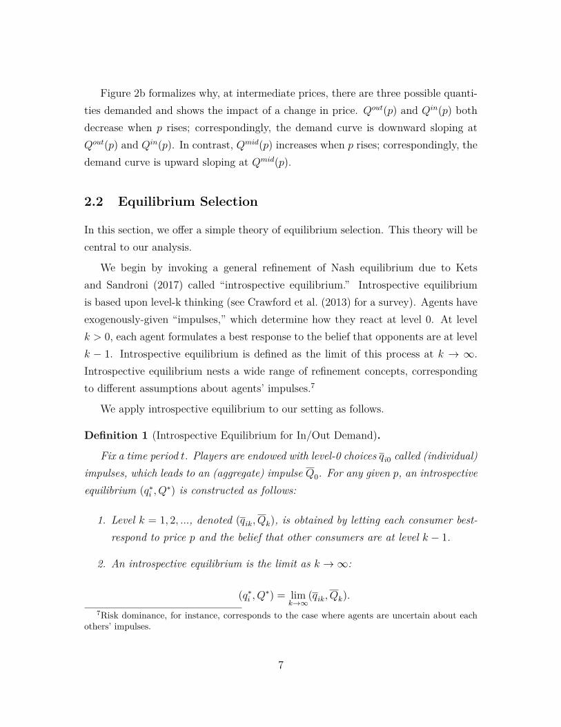
Figure 2b formalizes why, at intermediate prices, there are three possible quanti-ties demanded and shows the impact of a change in price. Qout(p) and Qin(p) bothdecrease when p rises; correspondingly, the demand curve is downward sloping atQout(p) and Qin(p). In contrast, Qmid(p) increases when p rises; correspondingly, thedemand curve is upward sloping at Qmid(p).

2.2 Equilibrium Selection

In this section, we offer a simple theory of equilibrium selection. This theory will becentral to our analysis.

We begin by invoking a general refinement of Nash equilibrium due to Ketsand Sandroni (2017) called “introspective equilibrium.” Introspective equilibriumis based upon level-k thinking (see Crawford et al. (2013) for a survey). Agents haveexogenously-given “impulses,” which determine how they react at level 0. At levelk > 0, each agent formulates a best response to the belief that opponents are at levelk − 1. Introspective equilibrium is defined as the limit of this process at k → ∞.Introspective equilibrium nests a wide range of refinement concepts, correspondingto different assumptions about agents’ impulses.7

We apply introspective equilibrium to our setting as follows.

Definition 1 (Introspective Equilibrium for In/Out Demand).

Fix a time period t. Players are endowed with level-0 choices qi0 called (individual)impulses, which leads to an (aggregate) impulse Q0. For any given p, an introspectiveequilibrium (q∗i , Q∗) is constructed as follows:

1. Level k = 1, 2, ..., denoted (qik, Qk), is obtained by letting each consumer best-respond to price p and the belief that other consumers are at level k − 1.

2. An introspective equilibrium is the limit as k →∞:

(q∗i , Q∗) = limk→∞

(qik, Qk).7Risk dominance, for instance, corresponds to the case where agents are uncertain about each

others’ impulses.

7

The impulses (qi0, Q0) play a key role in our model. To begin, we assume thateach agent’s impulse in period t is to do what she did in the previous period; that isqi0 = qt−1

i and Q0 = Qt−1. We take agents’ impulses in the first period as exogenousand denote them as q0

i and Q0.

Proposition 1 derives the introspective equilibrium as a function of the aggregateimpulse (Qt−1).

Proposition 1. Fix a time t and suppose the aggregate impulse is Qt−1. Whenpmin ≤ p ≤ pmax, the unique introspective equilibrium is:

Q∗(p,Qt−1

)=

Qin(p), if Qt−1 > Qmid(p).

Qmid(p), if Qt−1 = Qmid(p).

Qout(p), if Qt−1 < Qmid(p).

When p > pmax or p < pmin, Q∗ (p,Qt−1) is the unique solution to equation (3).

Proof of Proposition 1

The proof is easy to derive. Suppose first that pmin ≤ p ≤ pmax. From equation(3), we obtain the evolution of aggregate consumption between levels k and k + 1:

Qk+1 = 1− F (p− µ− αQk). (6)

Figure 3 corresponds to equation (6). It shows how, starting from an initial impulse(Qt−1), the aggregate consumption level evolves.

Observe that, if there is a high initial impulse to consume (Qt−1 > Qmid(p)),aggregate consumption increases between levels 0 and 1. Intuitively, the high levelof consumption at level 0 drives more agents to consume at level 1. Consumptioncontinues to increase between levels 2 and 3, 3 and 4, and so forth, reaching Qin(p) inthe limit. Hence, when Qt−1 > Qmid(p), the introspective equilibrium is Qin(p). Bya similar logic, aggregate consumption falls between successive levels when Qt−1 <

Qmid(p). When Qt−1 < Qmid(p), the introspective equilibrium is Qout(p).

8

Qk+1 = 1− F (p− µ− αQk)

Qk

Qk+1

1 – F(p – μ – α Qk)

Qt–1

Qk+1 = Qk

Qmid(p)Qout(p) Qin(p)Qt–1

Figure 3

Finally, when p > pmax or p < pmin, the proof follows from a similar argument.The only difference is that there is a single intersection in the analog of Figure 3.Q.E.D.

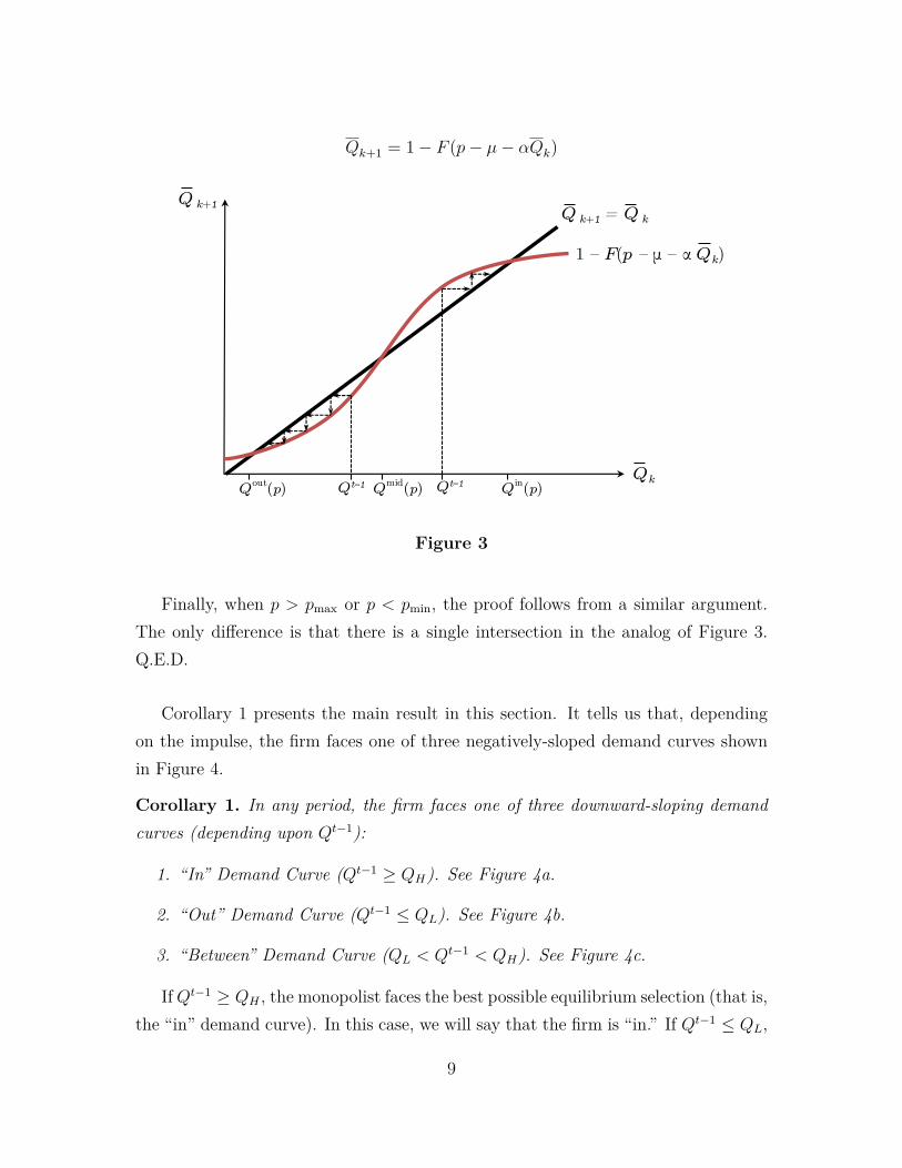
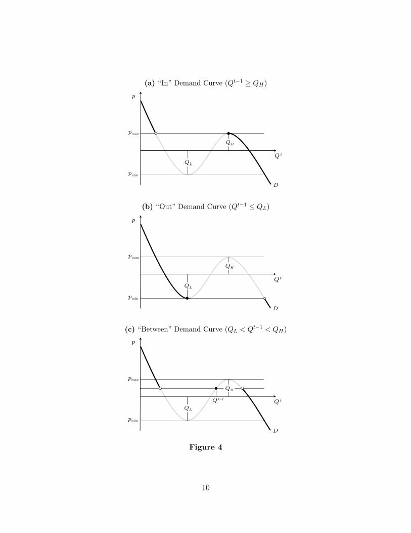
Corollary 1 presents the main result in this section. It tells us that, dependingon the impulse, the firm faces one of three negatively-sloped demand curves shownin Figure 4.

Corollary 1. In any period, the firm faces one of three downward-sloping demandcurves (depending upon Qt−1):

1. “In” Demand Curve (Qt−1 ≥ QH). See Figure 4a.

2. “Out” Demand Curve (Qt−1 ≤ QL). See Figure 4b.

3. “Between” Demand Curve (QL < Qt−1 < QH). See Figure 4c.

IfQt−1 ≥ QH , the monopolist faces the best possible equilibrium selection (that is,the “in” demand curve). In this case, we will say that the firm is “in.” If Qt−1 ≤ QL,

9

(a) “In” Demand Curve (Qt−1 ≥ QH)“In” Demand Curve (Q t–1 ≥ QH)

QH

QL

D

Q t

pmax

pmin

p

(b) “Out” Demand Curve (Qt−1 ≤ QL)“Out” Demand Curve (Q t–1 ≤ QL)

QH

QL

D

Q t

pmax

pmin

p

(c) “Between” Demand Curve (QL < Qt−1 < QH)“Between” Demand Curve: (QL < Q t–1 < QH)

QH

QL

D

Q t

pmax

pmin

p

Q t–1

Figure 4

10

the monopolist faces the worst possible equilibrium selection (that is, the “out”demand curve). In this case, we will say that the firm is “out.” And if QL <

Qt−1 < QH , the monopolist faces an intermediate equilibrium selection (that is, the“between” demand curve). In this case, we will say that the firm is “between.”

If, in period t, the firm sells no less than QH , we will say the firm ends the period“in.” Similarly, if the firm sells no more than QL, we will say that the firm ends theperiod “out.” And, if the firm sells an intermediate amount (QL < Qt < QH), wewill say that the firm ends the period “between.”

To illustrate the process of transitioning from “out” to “in,” suppose the firmbegins period t “out” (Qt−1 ≤ QL). If the firm sets a price above pmin, it will sell lessthan QL and consequently continue to face an “out” demand curve in period t+1. Ifinstead the firm sets a price below pmin, it will sell more than QH and consequentlyface an “in” demand curve in period t+ 1. This allows the firm to raise its price asfar as pmax in period t+ 1 without losing its “in” status.

2.3 Optimal Pricing

We are now in a position to formally state the monopolist’s problem and describeoptimal pricing.

Profits in period t (t = 1, 2, ..., T ) are πt = pt ·Qt, and Qt = Q∗(pt, Qt−1) (whereQ∗(pt, Qt−1) is defined as in Proposition 1). We take Q0, the initial consumptionlevel or impulse, as given. In each period, the monopolist chooses price to maximizethe discounted sum of future profits, using discount factor δ.

Case 1: the firm is myopic (δ = 0)

Here, the firm sets pt to maximize πt = pt ·Q∗(pt, Qt−1). Lemma 1 (stated below)says that, when the firm prices optimally, it ends period t either “in” or “out” — not“between.”

Lemma 1. If the firm is myopic (δ = 0) and prices optimally, it ends period t either“in” (Qt ≥ QH) or “out” (Qt ≤ QL).

The proof is simple. The only way for the firm to end period t “between” is if it

11

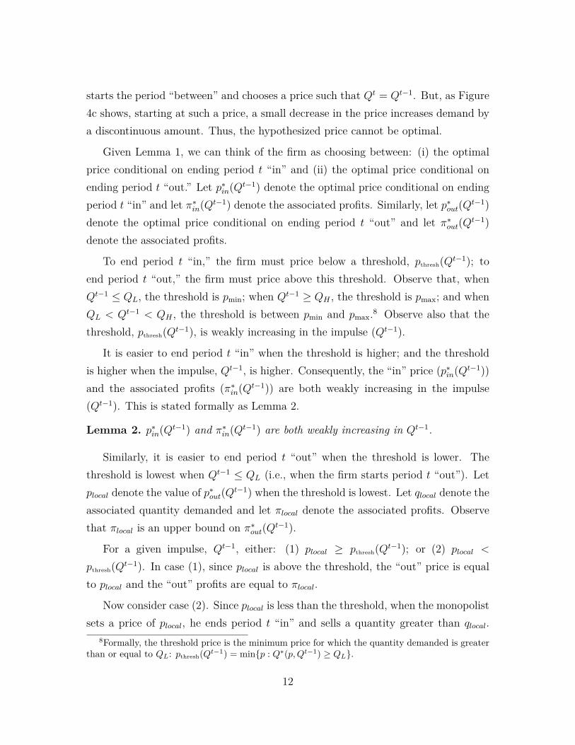
starts the period “between” and chooses a price such that Qt = Qt−1. But, as Figure4c shows, starting at such a price, a small decrease in the price increases demand bya discontinuous amount. Thus, the hypothesized price cannot be optimal.

Given Lemma 1, we can think of the firm as choosing between: (i) the optimalprice conditional on ending period t “in” and (ii) the optimal price conditional onending period t “out.” Let p∗in(Qt−1) denote the optimal price conditional on endingperiod t “in” and let π∗in(Qt−1) denote the associated profits. Similarly, let p∗out(Qt−1)denote the optimal price conditional on ending period t “out” and let π∗out(Qt−1)denote the associated profits.

To end period t “in,” the firm must price below a threshold, pthresh(Qt−1); toend period t “out,” the firm must price above this threshold. Observe that, whenQt−1 ≤ QL, the threshold is pmin; when Qt−1 ≥ QH , the threshold is pmax; and whenQL < Qt−1 < QH , the threshold is between pmin and pmax.8 Observe also that thethreshold, pthresh(Qt−1), is weakly increasing in the impulse (Qt−1).

It is easier to end period t “in” when the threshold is higher; and the thresholdis higher when the impulse, Qt−1, is higher. Consequently, the “in” price (p∗in(Qt−1))and the associated profits (π∗in(Qt−1)) are both weakly increasing in the impulse(Qt−1). This is stated formally as Lemma 2.

Lemma 2. p∗in(Qt−1) and π∗in(Qt−1) are both weakly increasing in Qt−1.

Similarly, it is easier to end period t “out” when the threshold is lower. Thethreshold is lowest when Qt−1 ≤ QL (i.e., when the firm starts period t “out”). Letplocal denote the value of p∗out(Qt−1) when the threshold is lowest. Let qlocal denote theassociated quantity demanded and let πlocal denote the associated profits. Observethat πlocal is an upper bound on π∗out(Qt−1).

For a given impulse, Qt−1, either: (1) plocal ≥ pthresh(Qt−1); or (2) plocal <

pthresh(Qt−1). In case (1), since plocal is above the threshold, the “out” price is equalto plocal and the “out” profits are equal to πlocal.

Now consider case (2). Since plocal is less than the threshold, when the monopolistsets a price of plocal, he ends period t “in” and sells a quantity greater than qlocal.

8Formally, the threshold price is the minimum price for which the quantity demanded is greaterthan or equal to QL: pthresh(Qt−1) = min{p : Q∗(p,Qt−1) ≥ QL}.

12

Since the quantity sold exceeds qlocal, the monopolist’s profits are also greater thanπlocal. Hence, a price of plocal results in a profit above πlocal (the upper bound on“out” profits). It follows that, in case (2), the “in” price yields a higher profit thanthe “out” price.

We conclude, therefore, that whenever the monopolist chooses the “out” priceover the “in” price, the “out” price is equal to plocal and the “out” profits are equalto πlocal. Lemma 3, stated below, summarizes.

Lemma 3. If the firm chooses to end period t “out,” it will set a price of plocal andearn a profit of πlocal.

Lemmas 2 and 3 imply that, if π∗in(Qt−1) > πlocal, the firm chooses the “in” priceand earns a profit of π∗in(Qt−1); otherwise, the firm chooses price plocal and earns aprofit of πlocal. Figure 5 illustrates the firm’s pricing problem (i.e., whether to chooseprice p∗in or plocal).9 Proposition 2 immediately follows.

Proposition 2. Suppose the firm is myopic (δ = 0). Depending upon the shape ofthe demand curve (which is a function of α, µ, and F ), there are three cases:

(i) It is optimal to go “in” in period t (choose pt such that Qt ≥ QH) regardless ofthe value of Qt−1.

(ii) It is optimal to go “out” in period t (choose pt such that Qt ≤ QL) regardlessof the value of Qt−1.

(iii) It is optimal for “in” (“out”) firms to stay “in” (“out”). “Between” firms go“in” (“out”) if Qt−1 is above (below) a cutoff (Qmyopic).

Instance (i) of Proposition 2 arises when π∗in(Qt−1) is greater than πlocal for allvalues of Qt−1. Instance (ii) arises when π∗in(Qt−1) is less than πlocal for all valuesof Qt−1. Instance (iii) arises when π∗in(Qt−1) > πlocal if and only if Qt−1 is above acutoff (Qmyopic).

9In the figure, p∗in is depicted as being right at the threshold for the firm to go “in” but p∗in mayalso be lower than that threshold.

13

Optimal Pricing: Myopic Case

(a) “Out” Demand Curve Qt−1 ≤ QL

D

p

Q̂Qlocal

plocal

pin*

(b) “Between” Demand Curve (QL < Qt−1 < QH)

D

p

Q̂Qlocal

plocal

Qt–1

pin*

(c) “In” Demand Curve Qt−1 ≥ QH

D

p

Q̂Qlocal

plocalpin*

Figure 5

14

Case 2: the firm is not myopic (δ > 0)

Proposition 3 compares the optimal pricing with that of a myopic firm.

Proposition 3. Suppose the firm is not myopic. In instances (i) and (ii) in Propo-sition 2, the firm acts as if it were myopic. In instance (iii), the firm potentiallyacts non-myopically in the first period, but acts myopically after that. Specifically,if Qnon-myopic < Q0 < Qmyopic, the firm charges a price below the myopic optimumin the first period so as to go “in” — a form of investment — and stays “in” in allsubsequent periods. If instead Q0 > Qmyopic (respectively, Q0 < Qnon-myopic), the firmbehaves as if it were myopic and in every period goes “in” (respectively, “out”).

Proof of Proposition 3

In instance (i), even if the firm disregarded the future, it would choose the “in”price over the “out” price for any initial impulse. Concern about the future onlymakes the firm more inclined to choose the “in” price, so it does not change thefirm’s behavior.

In instance (ii), the firm does not value having a higher impulse tomorrow: sincethe “out” profits (πlocal), which do not depend upon the impulse, always exceed the“in” profits. Consequently, the firm behaves as if it were myopic.

We now turn to instance (iii). Observe that a lower price today (weakly) benefitsthe firm tomorrow: since a lower price today results in a higher impulse-to-consumetomorrow. Consequently, concern about the future lowers the cutoff impulse forchoosing the “in” price over the “out” price. Q.E.D.

According to the proposition, the firm has an incentive to price below the myopiclevel in the first period in order to become “in” in subsequent periods — and reapthe associated benefits.10

The strategy of pricing low initially to become “in” seems to be commonplace.For instance, according to Adam Cohen, to build up its network in its early days,

10The switching-cost literature gives one reason why firms would want to price low initially: doingso builds up a set of locked-in consumers. Our framework shows an additional reason: even in theabsence of switching costs, pricing low initially builds up a product’s perceived popularity, via theimpulse.

15

PayPal “offered the service for free to both buyers and sellers and used millions ofdollars in VC funds to hand out bounties of five dollars to everyone who signedup...Handing out free money was costly, but fairly effective: by the end of 1999,PayPal had signed up twelve thousand registered users.”11,12

2.4 Influencers

Suppose there is an agent, called an “influencer,” who is connected to a fraction φ

of the consumers and has the ability to shift those consumers’ impulses: from “don’tconsume” to “consume” or vice-versa. Let b ∈ {0, 1} denote the influencer’s choicewhether to shift consumers’ impulses to “consume” or “don’t consume.”

The influencer can play a pivotal role in determining whether the firm is “in” or“out,” as the following corollary to Proposition 1 demonstrates.

Corollary 2. The firm faces

1. An “In” Demand Curve if:

(1− φ)Qt−1 + φb ≥ QH .

2. An “Out” Demand Curve if:

(1− φ)Qt−1 + φb ≤ QL.

3. A “Between” Demand Curve otherwise.

Given that influencers can help firms become — or stay — “in,” firms may bewilling to pay influencers for their services. An “out” firm can become “in” withouthelp from an influencer by dropping its price below pmin for one period; but this isexpensive. With help from an influencer, an “out” firm can become “in” without

11Cohen (2003), p. 228. PayPal raised its fees after building up its network. In 2017, the standardPayPal online transaction fee in the United States was 2.9% plus 30 cents. The “merchant rate”(available to those conducting $3,000 of business a month) was 1.9% plus 30 cents.

12This is by no means an isolated case. For example, in its “Free Basics Initiative,” Facebookoffers low-income consumers in developing countries free internet access to select websites.

16

dropping its price as much. In a competitive setting, an “in” firm might also pay aninfluencer in order to protect its “in” position against rivals (see Section 3 for furtherdiscussion of the competitive case).

In practice, one way in which an influencer might operate is by changing defaultoptions. Defaults appear to have the ability to alter consumer expectations — and/oract as nudges — and thereby affect initial impulses.

An illustration can be seen in the “browser war” in the 90s between the originally-dominant Netscape and Microsoft’s Internet Explorer. After initial difficulties topenetrate the market, Internet Explorer eventually managed to displace Netscape;and when this happened, it happened suddenly.13 The key to overtaking Netscapewas a deal between Microsoft and the internet provider AOL, whereby AOL agreedto set Internet Explorer as its default browser in exchange for valuable advertising.As Yoffie and Cusumano (1998) note: “To entice Steve Case, the CEO of AOL, tomake Internet Explorer AOL’s preferred browser, Gates offered to put an AOL iconon the Windows 95 desktop, perhaps the most expensive real estate in the world. Inexchange for promoting Internet Explorer as its default browser, AOL would havealmost equal importance with [AOL’s rival] MSN on future versions of Windows.” Tothis day, the browser wars continue, with smartphones being the latest battlefront.Here again, defaults appear to play a major role (e.g. Cain Miller (2012)).

Remark: Large Consumers

Suppose, in addition to small consumers, there is a large consumer who has theability to purchase a large quantity of the monopolist’s good. Like an influencer, alarge consumer can help tip the monopolist from “out” to “in.” Consequently, onewould expect the monopolist to pay the large consumer a rent — just as he wouldpay a rent to an influencer. This rent might take the form of a discount relative tothe price charged to small consumers.

We see such rents in the music streaming business, for instance. Services likeSpotify, Apple Music, and Tidal involve large network externalities. 14 It is not

13In the mid 1990s, Netscape controlled roughly 80% of the market; by the early 2000s, InternetExplorer controlled more than 90%.

14In this case, there are cross-good network externalities (see Section 5 for a formal discussion).

17

surprising, then, that both Apple Music and Tidal sought to challenge Spotify’sdominant position by signing big-name artists such as Beyonce, Drake, Frank Oceanand Kanye West, to exclusive deals on favorable terms to the artists. Accordingto Rolling Stone, “Superstar exclusives...have helped Apple and, to a lesser extent,Tidal generate millions of new customers, intensifying competition with Spotify.”15

3 Competition

It is a simple step to move from a monopoly setting to a competitive setting. Supposethere are two firms (1 and 2) that engage in price competition. At stage 1, firm 1sets price p1. At stage 2, firm 2 sets price p2.

We continue to assume there is a continuum of consumers (i ∈ [0, 1]) with tastesθi distributed F . Now, θi represents consumer i’s taste for good 1 relative to good2. Consumers make a binary choice whether to consume good 1 or good 2. Hence,overall demand, Q1 +Q2, sums to 1. The utility from consuming good 1 is θi + µ+α · Q1 − p1, where µ denotes the quality of good 1 relative to good 2. The utilityfrom consuming good 2 is α ·Q2 − p2.

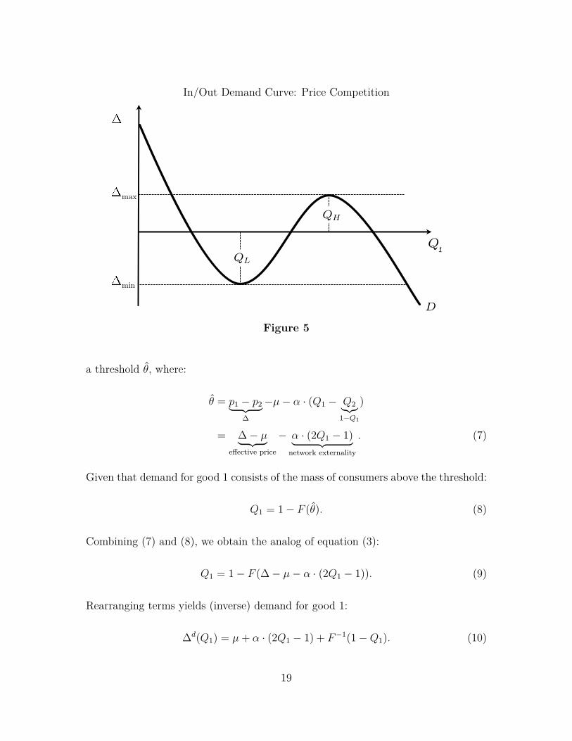
Under these assumptions, demand for each good depends upon the price differ-ential: ∆ = p1 − p2. We will focus on cases where the resulting demand curve isin/out, as pictured in Figure 5. Observe that, whenever demand for good 1 is in/out,demand for good 2 will also be in/out (given that Q2 = 1−Q1).16

We can use the same technique as before to derive a formula for demand. Observethat consumer i chooses good 1 over good 2 if and only if θi+µ+α·Q1−p1 ≥ α·Q2−p2.Therefore, the agents who consume good 1 are those whose taste for good 1 exceeds

An increase in the number of artists on a service makes it more attractive to users; a larger userbase, in turn, increases the willingness of artists to join a service.

15 Steve Knopper, “How Apple Music, Tidal Exclusives Are Reshaping Music Industry,” RollingStone, October 5, 2016, retrieved from http://www.rollingstone.com.

16Were we to plot the in/out demand curve for good 2, we would place p2 − p1 = −∆ on they-axis rather than ∆.

18

In/Out Demand Curve: Price Competition“In/Out” Demand Curve: Bertrand Competition

QH

QL

D

max

min

Q

1

Figure 5

a threshold θ̂, where:

θ̂ = p1 − p2︸ ︷︷ ︸∆

−µ− α · (Q1 − Q2︸︷︷︸1−Q1

)

= ∆− µ︸ ︷︷ ︸effective price

− α · (2Q1 − 1)︸ ︷︷ ︸network externality

. (7)

Given that demand for good 1 consists of the mass of consumers above the threshold:

Q1 = 1− F (θ̂). (8)

Combining (7) and (8), we obtain the analog of equation (3):

Q1 = 1− F (∆− µ− α · (2Q1 − 1)). (9)

Rearranging terms yields (inverse) demand for good 1:

∆d(Q1) = µ+ α · (2Q1 − 1) + F−1(1−Q1). (10)

19

Observe that a change in the quality of good 1 relative to good 2, µ, shifts demandvertically. Next, differentiating equation (10), we obtain a formula for the slope ofdemand:

d∆d(Q)1

dQ1= 2α︸︷︷︸

network externality

− 1f(F−1(1−Q1)) .︸ ︷︷ ︸

distribution of consumers’ tastes

(11)

As before, if F has support R and the pdf is single-peaked, there exists a thresholdα̂ > 0 such that:

1. Demand is downward-sloping if α ≤ α̂.

2. Demand is in/out if α > α̂.

Remark: Product Compatibility

It is easy to incorporate into our framework the idea that competing productsmay be more or less compatible.17 Suppose the utility from consuming good 1 isθi+µ+α·(Q1+γQ2)−p1 and the utility from consuming good 2 is α·(Q2+γQ1)−p2.The parameter γ ∈ [0, 1] represents the degree of compatibility of the goods; whenthey are more compatible, the consumers of good 1 derive more utility from theconsumption of good 2 (and vice-versa). The baseline model corresponds to the caseof perfect incompatibility (γ = 0).

This addition to the model has the following effect on the threshold for consuminggood 1:

θ̂ = ∆− µ− α(1− γ)︸ ︷︷ ︸“effective network parameter”

·(2Q1 − 1). (12)

The only change relative to the baseline model is that α(1 − γ) appears in place ofα. Hence, greater product compatibility (higher γ) is equivalent, from the point ofview of the firms, to smaller network externalities (lower α).

17The existing literature on network externalities has highlighted product compatibility as anissue of interest: particularly, the incentives of firms to make their products compatible (see, forinstance, Katz and Shapiro (1994)).

20

3.1 Equilibrium Selection

When the price differential ∆ is in an intermediate range, there are multiple Nashequilibria (Qout

1 (∆), Qmid1 (∆), and Qin

1 (∆)). To select between them, we will usethe same equilibrium refinement as in the single-firm case. This yields the followinganalog of Proposition 1.

Proposition 4. Fix a time t and suppose the aggregate impulse for firm 1 is Qt−11 .

When ∆min ≤ ∆ ≤ ∆max, the unique introspective equilibrium is:

Q∗1(∆, Qt−1

1

)=

Qin1 (∆), if Qt−1

1 > Qmid1 (∆).

Qmid1 (∆), if Qt−1

1 = Qmid1 (∆).

Qout1 (∆), if Qt−1

1 < Qmid1 (∆).

When ∆ > ∆max or ∆ < ∆min, Q∗1(∆, Qt−1

1

)is the unique solution to equation (9).

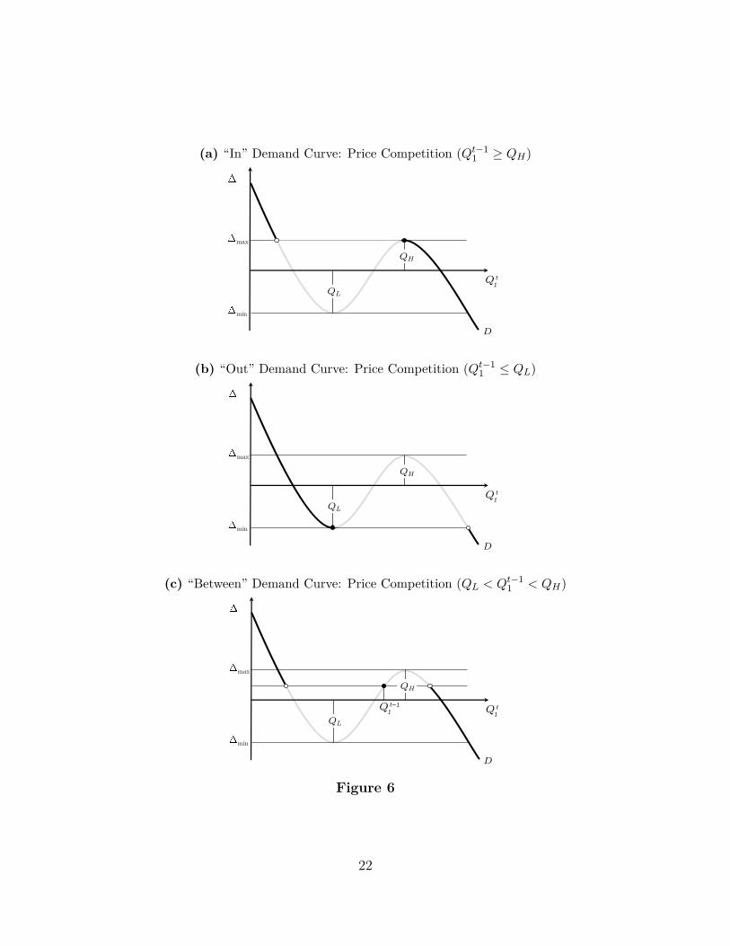
The following corollary to Proposition 4 is analogous to Corollary 1. It says thatfirm 1 faces one of the three negatively-sloped demand curves shown in Figure 6.

Corollary 3. In any period, firm 1 faces one of three downward-sloping demandcurves (depending upon Qt−1

1 ):

1. “In” Demand Curve (Qt−11 ≥ QH). See Figure 6a.

2. “Out” Demand Curve (Qt−11 ≤ QL). See Figure 6b.

3. “Between” Demand Curve (QL < Qt−11 < QH). See Figure 6c.18

We will again refer to a firm as “in,” “out,” or “between” depending upon whetherit faces an “in,” “out,” or “between” demand curve. Because overall demand is fixed(Q1 +Q2 = 1), either both firms are “between” or one is “in” and the other is “out.”

18From the demand curve for firm 1, it is easy to derive the demand curve for firm 2, as Q2 =1 −Q1. Note that firm 2 is “in” when Qt−1

2 ≥ 1 −QL, firm 2 is “out” when Qt−12 ≤ 1 −QH , and

firm 2 is “between” when 1−QH < Qt−12 < 1−QL.

21

(a) “In” Demand Curve: Price Competition (Qt−11 ≥ QH)“In” Demand Curve: Bertrand Competition (Q

t–1 ≥ QH) 1

QH

QL

D

max

min

Q t 1

(b) “Out” Demand Curve: Price Competition (Qt−11 ≤ QL)“Out” Demand Curve: Bertrand Competition (Q

t–1 ≤ QL) 1

QH

QL

D

max

min

Q t 1

(c) “Between” Demand Curve: Price Competition (QL < Qt−11 < QH)“Between” Demand Curve: Bertrand Competition (QL < Q

t–1 < QH) 1

QH

QL

D

max

min

Q t 1

Q t–1 1

Figure 6

22

We will focus attention in what follows on the case where firm 1 starts “in” andfirm 2 starts “out.” This corresponds to many cases of interest, where competitionis between an established firm that has built up a network and a recent entrant.

3.2 Analysis

We are now in a position to formally state and analyze the pricing game played bythe firms.

Recall that, at stage 1, firm 1 sets a price p1; at stage 2, firm 2 sets a price p2.The resulting payoffs to the firms are π1 = p1 · Qin

1 (∆) and π2 = p2 · (1 − Qin1 (∆)),

where ∆ = p1 − p2. Observe that π1 and π2 depend upon the shape of the demandcurve; the demand curve, in turn, depends upon parameters α, µ, and F .

We can use backward induction to solve for the equilibrium of the game. LetpBR2 (p1) denote firm 2’s best response to price p1 and let ∆(p1) = p1−pBR2 (p1). Firm1 chooses p1 to maximize:

π1(p1) = p1 ·Qin1 (∆(p1)).

Firm 1 “remains in” if ∆(p1) ≤ pmax and “falls out” if ∆(p1) > pmax. We willrefer to ∆(p1) ≤ pmax as the “remain-in constraint” or RIC. Demand for good 1decreases discontinuously when firm 1 falls out. Hence, there is an incentive for firm1 to choose a price that satisfies RIC. Furthermore — and most importantly — RICwill be a binding constraint in a region of the parameter space.

It is easy to show that, to remain in, firm 1 must set a price below a threshold pRIC

(the formal argument is given as part of the proof of Proposition 5 below). Therefore,the following is an equivalent formulation of the remain-in constraint:

p1 ≤ pRIC(α, µ, F ). (RIC)

Proposition 5 characterizes how a change in the goods’ relative qualities (µ) affectsthe equilibrium outcome in the region where RIC binds.

23

Proposition 5. When RIC binds, increases in the quality of good 1 relative to good2, as measured by µ:

1. Translate one-to-one into increases in good 1’s equilibrium price:

∂pRIC

∂µ= 1.

2. Have no effect on good 2’s equilibrium price.

3. Have no effect on equilibrium quantities (Q1 and Q2).

Proof of Proposition 5

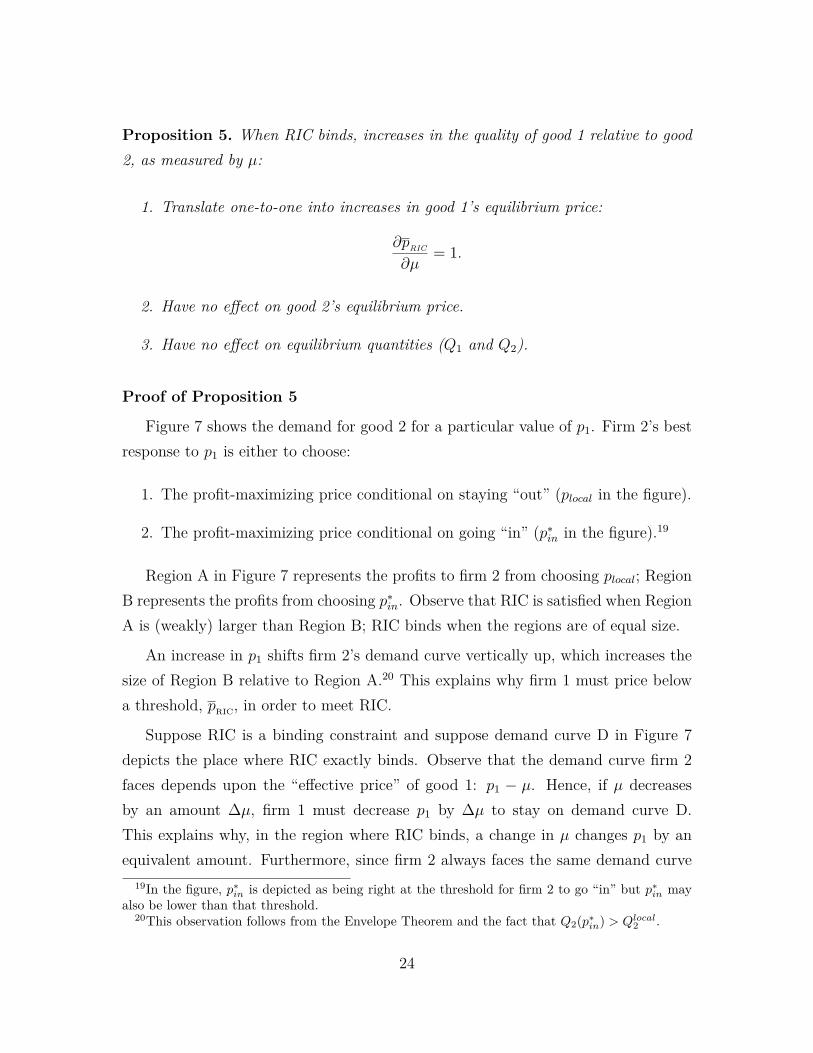
Figure 7 shows the demand for good 2 for a particular value of p1. Firm 2’s bestresponse to p1 is either to choose:

1. The profit-maximizing price conditional on staying “out” (plocal in the figure).

2. The profit-maximizing price conditional on going “in” (p∗in in the figure).19

Region A in Figure 7 represents the profits to firm 2 from choosing plocal; RegionB represents the profits from choosing p∗in. Observe that RIC is satisfied when RegionA is (weakly) larger than Region B; RIC binds when the regions are of equal size.

An increase in p1 shifts firm 2’s demand curve vertically up, which increases thesize of Region B relative to Region A.20 This explains why firm 1 must price belowa threshold, pRIC, in order to meet RIC.

Suppose RIC is a binding constraint and suppose demand curve D in Figure 7depicts the place where RIC exactly binds. Observe that the demand curve firm 2faces depends upon the “effective price” of good 1: p1 − µ. Hence, if µ decreasesby an amount ∆µ, firm 1 must decrease p1 by ∆µ to stay on demand curve D.This explains why, in the region where RIC binds, a change in µ changes p1 by anequivalent amount. Furthermore, since firm 2 always faces the same demand curve

19In the figure, p∗in is depicted as being right at the threshold for firm 2 to go “in” but p∗in mayalso be lower than that threshold.

20This observation follows from the Envelope Theorem and the fact that Q2(p∗in) > Qlocal2 .

24

The Remain-In Constraint (RIC)

D’Q2

plocal

Higher p1

D

p2 (Q )d2

Lower μ

Q2

localQ2

pin*

(p in)*

A

B

Figure 7

D in the region where RIC binds, it always charges the same price (plocal) and sellsthe same quantity (Qlocal

2 ). QED.

In practice, “in” firms may need to charge low — even zero — prices to satisfy theRIC constraint. For example, despite their overwhelming market shares, Google (inweb search), Uber (in ride sharing), and Amazon Web Services (in cloud computing)all keep their prices low — arguably to stunt the rise of their nearest rivals.21

Note that the “out” firm’s check on the “in” firm is a generalized form of “limitpricing,” whereby a monopolist is disciplined by a potential entrant. In our case,rather than deterring entry outright, the winning firm needs to deter the losing firmfrom becoming popular. It does so by allowing the losing firm to enjoy rents from asmall but loyal consumer base, a form of consolation prize.

21Note that one way in which online firms may charge users is by showing them advertisements.

25

3.3 Incentives for Innovation

The fact that when network externalities are large, the winning and losing firmscompete for the “in” position, as opposed to merely competing for a single marginalconsumer, has significant implications for the firms’ incentives to innovate.

To illustrate, suppose the two firms have an opportunity to invest up front onR&D activities that raise the intrinsic quality of their respective products. Let µidenote the intrinsic quality of firm’s i product, with µ = µ1 − µ2. Suppose qualityµi costs C (µi) to obtain, where C is twice differentiable and satisfies C ′, C ′′ > 0 andC ′ (0) = 0. Suppose µ1 and µ2 are observed by both firms before they engage in pricecompetition. (The exact timing of the choices of µ1 and µ2 is immaterial.)

Corollary 4 shows that, when the network externality is strong, the two firms faceradically different incentives to innovate:

Corollary 4. Consider the extended model with investments. Suppose firm 1 retainsthe “in” position and suppose that, in the pricing stage, the remain-in constraint isbinding (that is, the network externality is large). Then:

1. Firm 1’s optimal investment µ∗1 satisfies

C ′ (µ∗1) = Q∗1,

where Q∗1 denotes the equilibrium sales of firm 1.

2. Firm 2 has zero incentive to innovate.

This result follows from the fact that when the remain-in constraint is binding,we have dp1

dµ= 1. As a result, an increase in firm 1’s quality translates one-to-one into

an increase in its equilibrium price, and hence firm 1 invests in direct proportion tothe size of its own market (which, given its winning position, is large). In contrast,an increase in firm 2’s quality translates one-to-one into an reduction in its rival’sprice; thus, this higher quality has zero impact on firm 2’s revenues.

In practice, firms may also increase the quality of their products by acquiring star-tups with valuable product innovations. Indeed, such acquisitions are commonplace.

26

In the decade between 2008 and 2017, Google/Alphabet made 166 acquisitions, Ama-zon 51, Facebook 63, Ebay 31, Twitter 54, and Apple 66.22

Competition for the “in” position may lead to highly asymmetric outcomes. Toillustrate, suppose a third party (a “startup”) possesses an innovation and, prior toengaging in price competition, firms 1 and 2 bid in a (second-price) auction to buythe startup. Suppose the firm that acquires the startup adopts its innovation, andas a result improves its quality by ∆µ.

In this setting, provided the hypothesis of Corollary 4 is met, firm 1’s maximumbid for the startup is 2∆µQ1; whereas firm 2’s maximum bid is 0.23 Therefore, firm1 acquires the startup and pays 0 for it, further cementing it dominant position. Infact, in a multi-period version of this merger game in which a new startup emergesin every period, the dominant firm outbids its rival for each new startup; thus, itsdominant position becomes more and more entrenched as time goes by.

4 Piecewise Linear Demand

When consumers’ tastes follow a particular type of distribution (see Figure 8a), thein/out demand curve is piecewise linear. Figure 8b depicts the in/out demand curvefor a monopolist firm corresponding to Figure 8a.

Piecewise linear demand facilitates an analysis of the effects of demand volatility.Furthermore, it allows us to solve explicitly for the outcome of price competition.

22Consider a few of Apple’s acquisitions. PA Semi (purchased in 2008 for $278 million): aCalifornia-based chip designer whose acquisition was instrumental to Apple’s development of low-power processors. Siri (purchased in 2010 for $250 million): this virtual personal assistant technol-ogy has been integrated into a variety of Apple devices. C3 Technologies (purchased in 2011 for $273million): one of several startups acquired by Apple to improve its mapping features. PrimeSense(purchased in 2013 for $360 million): an Israeli 3D sensing company whose technology powers thefacial recognition features of the iPhone X.

23By winning, firm 1 not only increases its quality by ∆µ, it also prevents firm 2 from increasingits quality by ∆µ. Hence firm 1 is willing to bid 2∆µ per unit of expected sales.

27

(a) Pdf that gives rise to piecewise linear demand.

a

b

a

b

(b) Corresponding demand curve for the monopoly case (demand is in/out if α > 1v1+v2

).

p

1

D

1-av2

2v1

-1+av22v1

+ α+ μ

Q

12

[-a + α(1+a(v1+v2)] + μ

12

[a + α(1-a(v1+v2)] + μ

+ μ

Figure 8

28

4.1 Demand Volatility

Suppose, as in Section 2, there is a monopolist who maximizes expected profits,and suppose there is just a single pricing period (T = 1). Consumers’ tastes aredistributed as in Figure 8a and the network externalities are sufficiently large thatdemand is in/out (α > 1

v1+v2). In contrast to Section 2, µ (the quality of the mo-

nopolist’s good relative to the outside option) is a random variable: µ = µ̂ + ε,where:

ε =

σ, with probability r.

−σ, with probability r.

0 with probability 1− 2r.

The resulting demand curve, pd(Q), has a random component:

pd(Q) = p̂(Q) + ε.

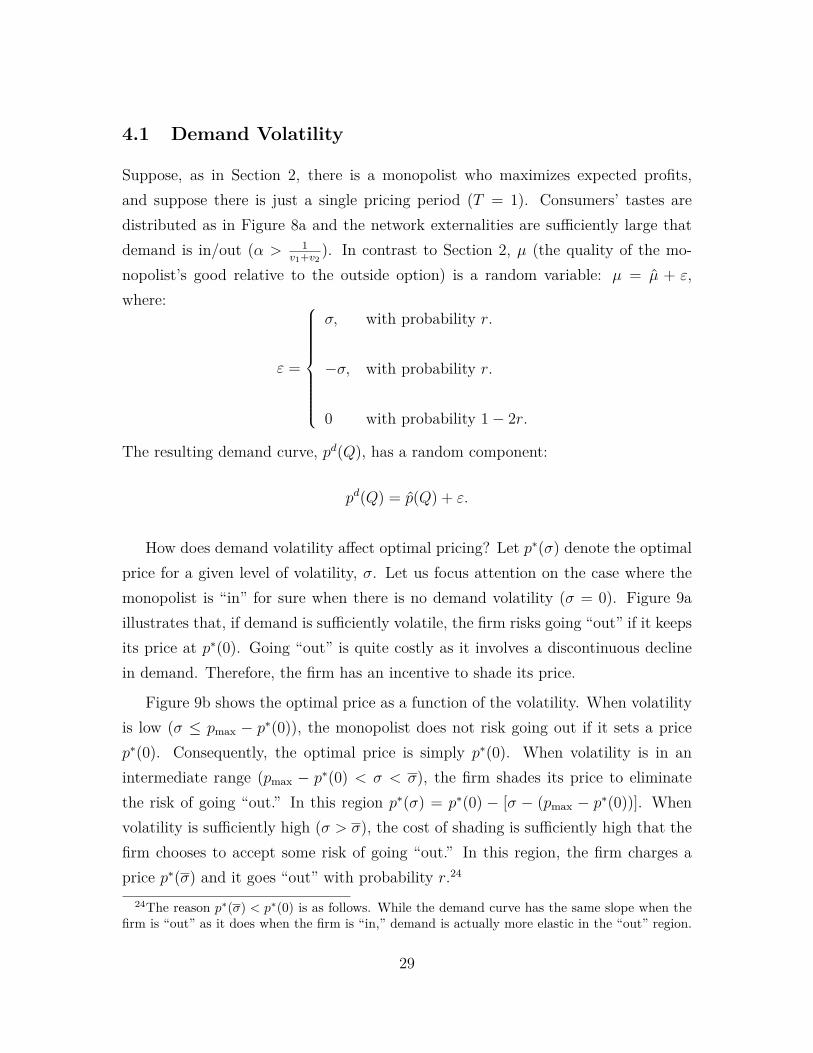
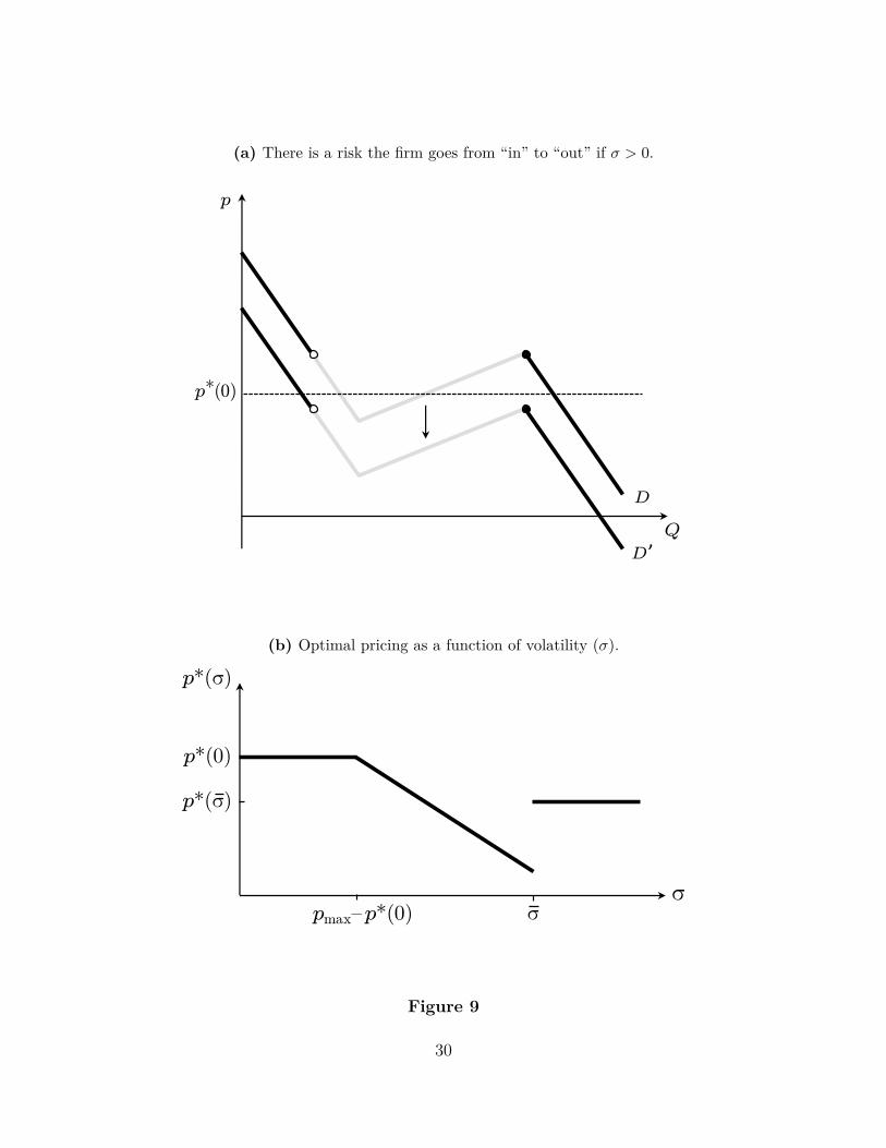
How does demand volatility affect optimal pricing? Let p∗(σ) denote the optimalprice for a given level of volatility, σ. Let us focus attention on the case where themonopolist is “in” for sure when there is no demand volatility (σ = 0). Figure 9aillustrates that, if demand is sufficiently volatile, the firm risks going “out” if it keepsits price at p∗(0). Going “out” is quite costly as it involves a discontinuous declinein demand. Therefore, the firm has an incentive to shade its price.

Figure 9b shows the optimal price as a function of the volatility. When volatilityis low (σ ≤ pmax − p∗(0)), the monopolist does not risk going out if it sets a pricep∗(0). Consequently, the optimal price is simply p∗(0). When volatility is in anintermediate range (pmax − p∗(0) < σ < σ), the firm shades its price to eliminatethe risk of going “out.” In this region p∗(σ) = p∗(0) − [σ − (pmax − p∗(0))]. Whenvolatility is sufficiently high (σ > σ), the cost of shading is sufficiently high that thefirm chooses to accept some risk of going “out.” In this region, the firm charges aprice p∗(σ) and it goes “out” with probability r.24

24The reason p∗(σ) < p∗(0) is as follows. While the demand curve has the same slope when thefirm is “out” as it does when the firm is “in,” demand is actually more elastic in the “out” region.

29

(a) There is a risk the firm goes from “in” to “out” if σ > 0.

D

Q

p

p (0)*

D’

(b) Optimal pricing as a function of volatility (σ).

σ

p*(σ)

σpmax–p*(0)

p*(0)

p*(σ)

Figure 9

30

Equilibrium Outcome: Piecewise Linear Demand

μ

Q1 = 0Δ >Δmax

α

+

Q1 = 1

RIC binds

RIC loose

Δ =Δmax

αmaxαmin

+

Firm 1 remains in

π1(μ, α), π2(μ, α)

Firm 1 falls out

+ ? – ?

Figure 10

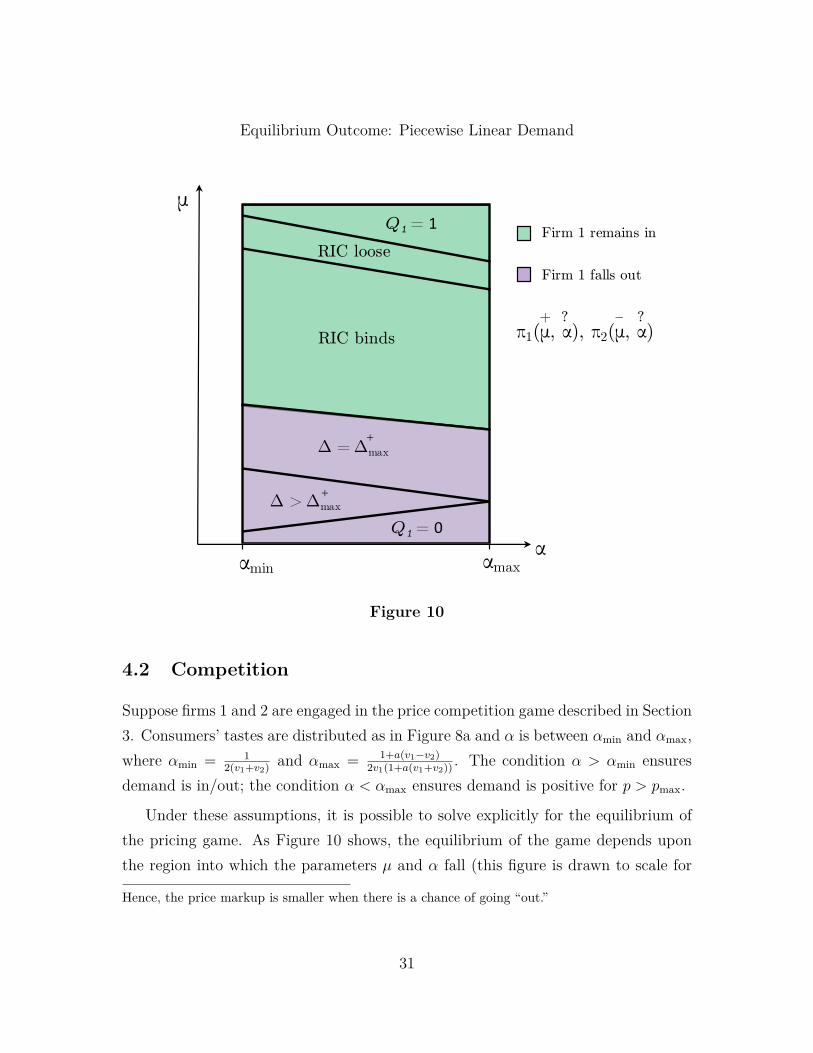
4.2 Competition

Suppose firms 1 and 2 are engaged in the price competition game described in Section3. Consumers’ tastes are distributed as in Figure 8a and α is between αmin and αmax,where αmin = 1

2(v1+v2) and αmax = 1+a(v1−v2)2v1(1+a(v1+v2)) . The condition α > αmin ensures

demand is in/out; the condition α < αmax ensures demand is positive for p > pmax.

Under these assumptions, it is possible to solve explicitly for the equilibrium ofthe pricing game. As Figure 10 shows, the equilibrium of the game depends uponthe region into which the parameters µ and α fall (this figure is drawn to scale for

Hence, the price markup is smaller when there is a chance of going “out.”

31

the case where a = 1 and v1 = v2 = 13).25

Several points are worth making. First, as one would expect, firm 1 “remains in”if µ (good 1’s relative quality) is above a threshold; firm 1 “falls out” if µ is belowthe threshold. The remain-in constraint (RIC) is binding when µ is just above thethreshold. When µ is just below the threshold, firm 2 chooses the minimal price thatputs it “in” (∆ = ∆+

max).

Second, as one crosses the threshold from the region where RIC is satisfied to theregion where RIC is violated, prices jump discontinuously. Firm 1’s price jumps upand firm 2’s price jumps down. Intuitively, prices jump because firm 1 gives up onremaining “in” and firm 2 decides it is worthwhile to go “in.”

Third, competition between the firms is “normal” in the regions where RIC isloose and where ∆ > ∆+

max. Here, changes in relative quality, µ, impact the prices andquantities of both goods. Competition is abnormal when RIC binds or ∆ = ∆+

max.In those regions, changes in µ have no effect on quantities and only affect firm 1’sprice.

Finally, one might think that the firm that ends up “in” benefits from an increasein network externalities (α). In fact, it is ambiguous whether an increase in α benefitsor hurts the “in” firm. The reason is as follows. An increase in α has two effects(which are illustrated in Figure 11):

1. For a given price differential, the “in” firm gets a larger share of the market.

2. Demand is more elastic.

The “in” firm benefits from the first effect. The second effect, however, can drivemore intense competition between the firms for the “in” position. This competitionmay be harmful to the “in” firm. A lesson is that, even in cases where one firm hasa dominant market share, it may be incorrect to assume that competition is weak.

25Proposition 6, stated in the Appendix, specifies the equilibrium prices and quantities in eachregion.

32

How an increase in α affects demand.

Δ

1

D

D’

Q1

Higher α

Figure 11

5 Multiple Goods and Platforms

It is easy to extend our model to the case of a multi-sided platform, where a firmsells multiple goods and there are cross-good externalities. One example is Uber,which sells two goods: passenger rides and driver rides. Passengers care about thenumber of drivers; drivers, similarly, care about the number of passengers.

Suppose the monopolist sells two goods (j = 1, 2). There are two populations ofconsumers (1, 2) with a continuum of consumers in each population; consumers inpopulation j are potential consumers of good j. Each consumer has a type θ; the θ’sare distributed Fj for good j. Consumer i’s utility from consuming good j is:

θi + µj + αj ·Qj + βj ·Ql − pj,

where pj denotes the price of good j, µj denotes the intrinsic quality of good j,the term αj · Qj represents a same-good network externality, and the term βj · Ql

represents a cross-good network externality. As before, we normalize to zero theutility from not consuming.

33

The following is an analog of equation (3):

Qj = 1− Fj(pj − µj − αj ·Qj − βj ·Ql). (13)

From equation (13), we obtain a formula for (inverse) demand:

pDj (Qj, Ql) = F−1j (1−Qj) + αj ·Qj + βj ·Ql + µj. (14)

Consider the simple “symmetric” case where α1 = α2 = α, β1 = β2 = β, andF1 = F2. In addition, suppose the two goods have equal initial impulses: Q0

1 = Q02 =

Q0.

Provided a suitable concavity assumption is satisfied, the firm sets a single price:p1 = p2 = p. In this case, the model is isomorphic to the baseline model with a singlegood, with α + β appearing in place of α.26

Remark

This framework is amenable to analyzing platform competition as well. We canthink about consumers of good 1 (good 2) choosing whether to purchase good 1 (good2) from firm 1 or firm 2. One can think, for instance, about competition betweenUber and other ride-sharing apps like Lyft. Our result from Section 3 that firmsare not asleep has an analog in this context and can explain why Uber, despite itsdominant position, is constantly working to improve the quality of its service.

6 Conclusion

We proposed a rich yet tractable framework to study optimal pricing and pricecompetition in the presence of network effects.

A critical feature of markets with networks externalities is their ability to generatemultiple equilibria. Such multiplicity is behind large asymmetries between winners

26As noted in the literature, there is often asymmetric pricing (p1 6= p2) in two-sided markets (seeespecially Rochet and Tirole (2003)). Such pricing is optimal, for example, when the cross-networkexternalities are asymmetric (β1 6= β2). We leave this extension for future work.

34

and losers. It is also behind the apparent paradox that it is difficult to become awinner, and yet the winning position is fragile; hence, winners are not asleep.

Understanding how one equilibrium gets picked over another is essential. Weproposed a simple theory of equilibrium selection that captures the notion that afirm’s popularity exhibits a form of inertia over time, and is affected as well bysalient consumers that are popular among their peers. A firm’s default popularity,inherited from the previous period, then determines whether it currently faces itsworst possible demand curve (the “out” demand), its best possible curve (the “in”demand), or an intermediate version of the two (the “between” demand). Eachof these demand curves has a well-behaved shape with a standard negative slope,but with a discontinuity. This simple classification immediately sheds light on thefirm’s optimal pricing, its equilibrium transitions between the losing and the winningpositions, and its incentives for innovation.

Our model features a form of asymmetric competition in which winning and losingfirms co-exist, with the losing firm keeping the winning firm in check. This check onthe winning firm is a generalized form of “limit pricing,” whereby a monopolist isdisciplined by a potential entrant. In our case, rather than deterring entry outright,the winning firm needs to deter the losing firm from becoming popular. It does soby allowing the losing firm to enjoy rents from a small but loyal consumer base, aform of consolation prize.

For the interested reader, Appendix B analyzes a simple version of the modelwhere all consumers are of the same type. This version gives the starkest case whereimpulses play a role; but it lacks the richness of the in/out demand curve.

In subsequent work, we expect to propose a method for valuing firms in thepresence of network effects, with such effects opening the possibility of large profitsfor popular firms, but also leading to the risk of sudden failure.

35

Appendix

A Competition when Demand is Piecewise-Linear

Consider the pricing game described in Section 3 and suppose demand is piecewise-linear (as in Figure 8). Proposition 6, proven in the Online Supplement, describesthe equilibrium outcome.27

Proposition 6. The equilibrium of the pricing game depends upon which regionparameters µ and α fall into. There are six regions which can be ordered from ahighest-µ region to a lowest-µ region:

1. RIC is loose and Q∗1 = 1 (µ ≥ µ1):

p∗1 = µ+ α + −1 + av2

2v1,

p∗2 = 0.

2. RIC is loose and Q∗1 < 1 (µ1 > µ ≥ µ2):

p∗1 = 12µ−

32α + 3 + av2

4v1,

p∗2 = −14µ−

54α + 5− av2

8v1,

Q∗1 = v1

2(1− 2v1α)(12µ−

32α + 3 + av2

4v1).

27The Online Supplement is available at: http://www.robertakerlof.com/research.html.

36

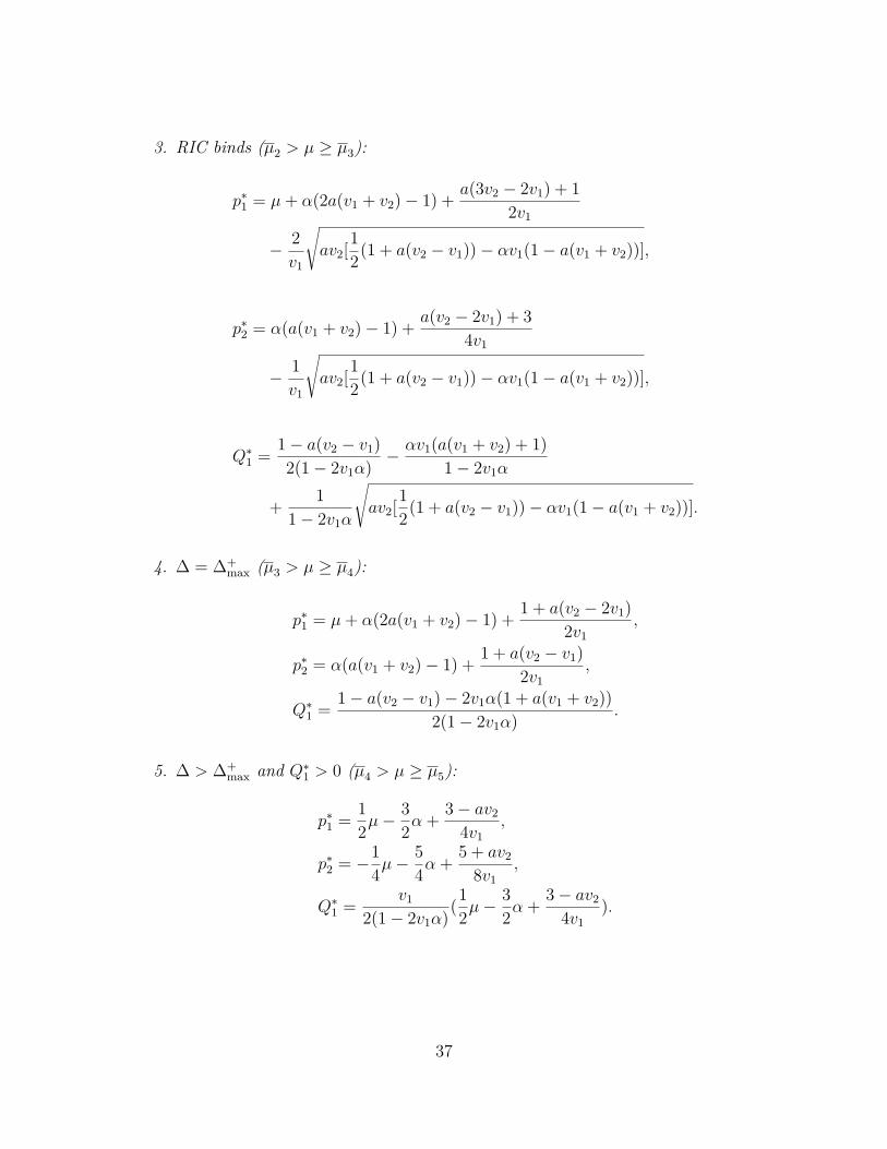
3. RIC binds (µ2 > µ ≥ µ3):

p∗1 = µ+ α(2a(v1 + v2)− 1) + a(3v2 − 2v1) + 12v1

− 2v1

√av2[12(1 + a(v2 − v1))− αv1(1− a(v1 + v2))],

p∗2 = α(a(v1 + v2)− 1) + a(v2 − 2v1) + 34v1

− 1v1

√av2[12(1 + a(v2 − v1))− αv1(1− a(v1 + v2))],

Q∗1 = 1− a(v2 − v1)2(1− 2v1α) −

αv1(a(v1 + v2) + 1)1− 2v1α

+ 11− 2v1α

√av2[12(1 + a(v2 − v1))− αv1(1− a(v1 + v2))].

4. ∆ = ∆+max (µ3 > µ ≥ µ4):

p∗1 = µ+ α(2a(v1 + v2)− 1) + 1 + a(v2 − 2v1)2v1

,

p∗2 = α(a(v1 + v2)− 1) + 1 + a(v2 − v1)2v1

,

Q∗1 = 1− a(v2 − v1)− 2v1α(1 + a(v1 + v2))2(1− 2v1α) .

5. ∆ > ∆+max and Q∗1 > 0 (µ4 > µ ≥ µ5):

p∗1 = 12µ−

32α + 3− av2

4v1,

p∗2 = −14µ−

54α + 5 + av2

8v1,

Q∗1 = v1

2(1− 2v1α)(12µ−

32α + 3− av2

4v1).

37

6. ∆ > ∆+max and Q∗1 = 0 (µ < µ5):

p∗1 = 0,

p∗2 = −µ+ α− 1− av2

2v1.

The cutoffs between regions are defined as follows:

µ1 = 5− av2

2v1− 5α,

µ2 = 1− a(5v2 − 4v1)2v1

− α(4a(v1 + v2) + 1)

+ 4v1

√av2[12(1 + a(v2 − v1))− αv1(1− a(v1 + v2))],

µ3 = 1− a(5v2 − 4v1)2v1

− α(1 + 4a(v1 + v2))

+ 1 + 3a(v2 − v1)− 2αv1(1− 3a(v1 + v2))v1[1 + a(v2 − v1) + 2αv1(−1 + a(v1 + v2))]×√av2[12(1 + a(v2 − v1))− αv1(1− a(v1 + v2))],

µ4 = 1− a(3v2 − 4v1)2v1

− α(4a(v1 + v2) + 1),

µ5 = −3 + av2

2v1+ 3α.

38

B A Simple Case: Homogeneous Consumers

Here, we analyze a simple version of the model where all consumers are of the sametype, and therefore aggregate demand is either 0 or 1. This version gives the starkestcase where impulses play a role.

Monopoly

First, consider the monopoly setting. Under the assumption that all consumersare of type θ = 0, demand in period t is given by:

Qt(pt, Qt−1

)=

1, if pt ≤ µ+ αQt−1.

0, if pt > µ+ αQt−1.

The monopolist faces an “in” demand curve in period t if Qt−1 = 1, an “out”demand curve in period t if Qt−1 = 0, or a “between” demand curve in period t if0 < Qt−1 < 1.

Suppose, as in Section 2, that the monopolist chooses a price in each of T periodsand has a discount factor of δ. Let us solve for the optimal choice of prices.

From Proposition 3, it follows that we can restrict attention to two possiblepricing strategies. Strategy 1: go “in” in period 1 and stay “in” in subsequentperiods. Strategy 2: go “out” in period 1 and stay “out” in subsequent periods.

Strategy 1 involves setting a price p1 = µ + αQ0 in the first period and a pricept = µ+α in subsequent periods (t > 1). The profits associated with this strategy are:∑Tt=1 δ

t−1pt = µ+ α(Q0 + δ−δT

1−δ

). Strategy 2 yields a payoff of 0 to the monopolist.

The monopolist will follow Strategy 1 if and only if it yields nonnegative profits,or:

µ ≥ −α(Q0 + δ − δT

1− δ

)

If the monopolist’s good is of sufficiently high quality (µ ≥ −α(δ−δT

1−δ

)), the

monopolist chooses to go “in” (i.e., follow Strategy 1) regardless of consumers’

39

initial impulse. Similarly, if the monopolist’s good is of sufficiently low qualityµ < −α

(1 + δ−δT

1−δ

), the monopolist chooses to go “out” (i.e., follow Strategy 2)

regardless of consumers’ initial impulse.

If the quality of the monopolist’s good is in an intermediate range (−α(δ−δT

1−δ

)>

µ ≥ −α(1 + δ−δT

1−δ

)), the monopolist’s strategy depends upon the impulse. The

monopolist chooses to go “in” (follow Strategy 1) if and only if the initial impulse toconsume is above a threshold: Q0 ≥ −

(µα

+ δ−δT

1−δ

).

Observe that an increase in the number of time periods (T ) makes the monopolistmore inclined to go “in” (i.e., it decreases the threshold quality for following Strategy1). This is intuitive since the monopolist will be more willing to pay an initial costof going “in” when there are more subsequent periods in which to reap the rewards.

Competition

Now, consider a competitive setting. As in Section 3, assume that firm 1 choosesits price in stage 1 and firm 2 chooses its price in stage 2. If all consumers are oftype θ = 0, demand for good 1 is given by:

Q1(∆, Q0

1

)=

1, if ∆ ≤ µ+ α(2Q0

1 − 1).

0, if ∆ > µ+ α(2Q01 − 1).

Assume firm 1 starts “in” (Q01 = 1) and sets its price before firm 2.

We can analyze the game by backward induction. Given p1, firm 2 can either setp2 ≥ p1 − µ− α, in which case it gets zero demand and receives a payoff of zero, orit can get all of the demand by setting a price just below p1−µ−α, in which case itreceives a payoff of p1−µ−α. It is optimal for firm 2 to price just below p1−µ−αif and only if p1 − µ− α > 0.

Hence, to deter firm 2 from taking the whole market, firm 1 must set a pricep1 = µ+α. Therefore, firm 1 has a choice between setting a price above µ+α, withan associated payoff of 0, or setting p1 = µ+ α, with an associated payoff of µ+ α.

Firm 1 will set p1 = µ+α, taking the whole market, if and only if µ ≥ −α. When

40

µ < −α, firm 2 will take the whole market.

Observe that good 2’s quality must exceed good 1’s quality by an amount α inorder for firm 2 to take the market (recall that µ denotes the relative quality of goods1 and 2). The reason is that firm 1 has an advantage from starting “in.” The size ofthis advantage is increasing in the network effect (α).

41

References

Armstrong, Mark, “Competition in two-sided markets,” RAND Journal of Eco-nomics, 2006, 37 (3), 668–691.

Becker, Gary S., “A note on restaurant pricing and other examples of social influ-ences on price,” Journal of Political Economy, 1991, 99 (5), 1109–1116.

Cain Miller, Claire, “Browser Wars Flare Again, on Little Screens,” The NewYork Times, December 9, 2012.

Cohen, Adam, The Perfect Store: Inside eBay, Back Bay Books, 2003.

Crawford, Vincent P., Miguel A. Costa-Gomes, and Nagore Iriberri,“Structural models of nonequilibrium strategic thinking: Theory, evidence, andapplications,” Journal of Economic Literature, 2013, 51 (1), 5–62.

Farrell, Joseph and Paul Klemperer, “Coordination and lock-in: Competitionwith switching costs and network effects,” Handbook of industrial organization,2007, 3, 1967–2072.

Fudenberg, Drew and Jean Tirole, “Pricing a network good to deter entry,” TheJournal of Industrial Economics, 2000, 48 (4), 373–390.

Gaskins, Darius W., “Dynamic limit pricing: Optimal pricing under threat ofentry,” Journal of Economic Theory, 1971, 3, 306–322.

Katz, Michael L. and Carl Shapiro, “Network externalities, competition, andcompatibility,” The American Economic Review, 1985, 75 (3), 424–440.

and , “Systems competition and network effects,” The Journal of EconomicPerspectives, 1994, 8 (2), 93–115.

Kets, Willemien and Alvaro Sandroni, “A Theory of Strategic Uncertainty andCultural Diversity,” Working Paper, 2017.

Klemperer, Paul, “Markets with consumer switching costs,” Quarterly Journal ofEconomics, 1987, 102 (2), 375–394.

42

, “Competition when consumers have switching costs: An overview with applica-tions to industrial organization, macroeconomics, and international trade,” Reviewof Economic Studies, 1995, 62 (4), 515–539.

Milgrom, Paul and John Roberts, “Limit Pricing and Entry under IncompleteInformation: An Equilibrium Analysis,” Econometrica, 1982, 50 (2), 443–459.

Rochet, Jean-Charles and Jean Tirole, “Platform competition in two-sidedmarkets,” Journal of the European Economic Association, 2003, 1 (4), 990–1029.

and , “Two-sided markets: a progress report,” RAND Journal of Economics,2006, 37 (3), 645–667.

Weyl, E Glen, “A price theory of multi-sided platforms,” American EconomicReview, 2010, 100 (4), 1642–72.

Yoffie, David B. and Michael A. Cusumano, Competing on Internet time:lessons from Netscape and its battle with Microsoft, Simon and Schuster, 1998.

43