Embed Size (px)
Citation preview

1
Access Network DesignAccess Network Design
David TipperAssociate ProfessorAssociate Professor
Graduate Telecommunications and Networking Program
U i it f Pitt b hUniversity of PittsburghSlides 6
http://www.sis.pitt.edu/~dtipper/2110.htmlhttp://www.sis.pitt.edu/~dtipper/2110.html
Network Design Categories
• Remember network design classifications
Network DesignSize
Metro AccessWAN
Wired
Size
Wired Wireless. . . . . . . . . .
Technology
Stage
TELCOM 2110 2
VPN. . . . . . . . . .
greenfield greenfield incremental
Stage
Techniques used to design the network will depend on the classification Consider Access Network Design (wired and wireless) for the greenfield case
2
Access, Metro and Long-Haul Transport
WAN Long-haul network Access network
• Access networks connect “small” sites to the WAN/Metro network
Access networks are the “ends”– Access networks are the ends and “tails” of networks (last mile networks)
– often represents most of the total network cost, (e.g., residential telephone network)
• Variety of Technologies:– Wireless LANs
TELCOM 2110 3
Metro networkSource: J. Doucette, Ph.D. Thesis, UofA, 2004
– Cellular networks
– WiMAX
– Cable networks
– Copper Local loop / DSL
– Fiber to home/curb
– Power Line Com.
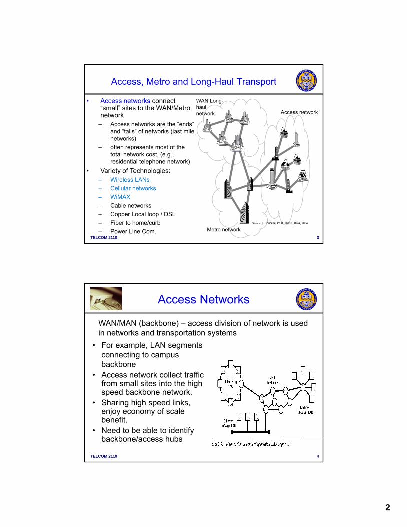
Access Networks
WAN/MAN (backbone) – access division of network is used in networks and transportation systems
F l LAN t• For example, LAN segments connecting to campus backbone
• Access network collect traffic from small sites into the high speed backbone network.
• Sharing high speed links
TELCOM 2110 4
• Sharing high speed links, enjoy economy of scale benefit.
• Need to be able to identify backbone/access hubs

3
Access Network Design
• Traffic Matrix– Specifies traffic between all source-destination pairs
Entry T is the traffic from source i to destination j– Entry Tij is the traffic from source i to destination j– Source and destination maybe host, LAN, etc.– Developed in conceptual design- usually based on
peak busy hour
• Cost Matrix– Cost of link capacity Cij between nodes i and j
C ff C ( )
TELCOM 2110 5
– Cost may depend on traffic demand w needed Cij(w)
• Nodal Weight– The total traffic at a node
• sum of all traffic in and out of the node
Nodal Weight
• Given a set of sites/nodes Ni and traffic matrix T,
– Weight(Ni) = j (Ti,j+Tj,i).Mean data rate demands
Dallas Denver Vienna
j ,j j,– Weight of a site is the sum of all traffic
in and out of the site– Link Capacity needed is proportional to
weight • Example of corporation in Dallas,
Vienna, and DenverWeight(Dallas) = 2.2 + 2.8 = 5.0 MbpsWeight(Denver) = 1.1 + 1.6 = 2.7 MpbsWeight(Vienna) = 4.0+ 2.9 = 6.9 Mbps
Dallas -----------.1Mb
2.1 Mb
Denver .3 Mb ---------------
.8Mb
TELCOM 2110 6
Weight(Vienna) 4.0 2.9 6.9 Mbps
• Note a node/site weight can indicates natural traffic centers for access to backbone locations Vienna 2.5 Mb 1.5 Mb ------------

4
Backbone/Access/Hub Sites
• Design Principle – Compute the weight of all the nodes to determine if there are
natural traffic centers • Example of corporation - Vienna has largest weight
– Nodes with largest weights are potential access points to backbone (e.g., MAN or WAN) networks
– Generally acceptable for small weight nodes to route their traffic via big weight nodes, but we do not want to route the traffic between big nodes via the small nodes
– Not always obvious what is big and small nodeWant large difference in weight between the big and small
TELCOM 2110 7
• Want large difference in weight between the big and small
• Weights can also be used to partition problem into two parts– Access network design– Backbone design
Access Network Design
• Can roughly categorize access network design (AND) problems IBM VLR
HLR
AUC EIR
( ) p ob e s– One speed one center
design• For example, local loop in
telephone network
– Multi-speed access design• For example, LAN design
from variety of hosts
M lti t D i
MSC
BS2
BS3
BS4
SD
Centillion 1400Bay Networks
ETHER RS 232C
PC C ARD
P* 8x50OOO130A O N
6
I NS ACT ALMRST
LIN K
PWR ALM FAN0 FAN1 PWR0 PWR1
ALM
BSC
BS3
SD
Centillion 1400Bay Networks
ETHER RS 232C
PC C ARD
P* 8x50OOO130A O N
6
I NS ACT ALMRST
LIN K
PWR ALM FAN0 FAN1 PWR0 PWR1
ALM
BSC
SD
Centillion 1400Bay Networks
ETHER RS 232C
PC CARD
P*8x50OOO130A O N6
INS ACT ALMRST LI NK
PWR ALM FAN0 FAN1 PW R0 PWR1
ALM
BSC
VLR
TELCOM 2110 8
– Multi-center Design• For example, cellular
networks with multiple base station controllers
• Historically informal back of the envelope design procedures, becoming more mathematical based
BS7BS5
BS1
BS6BS7
BS5
BS2 BS4
BS1
BS6
Reference R. Cahn, Wide Area NetworkDesign: Concepts and Tools for OptimizationMorgan Kaufmann ,1998 Ch 5, 6

5
One-speed One-Center Design
Problem: Connecting sites to one backbone node (switch, router) all links with the same capacity
OR OR
TELCOM 2110 9
Approaches
• Shortest Path Tree (Dijkstra’s Algorithm)– Expensive, low utilizaton, good delay
• Minimum Spanning Tree (Prim’s Algorithm)– Cheap, possibly high delay due to longer path length
• Comprise (Prim-Dijkstra Algorithms)– Better results, harder to determine
• Exhaustive Search (consider all possible trees)
TELCOM 2110 10
( p )– Cayley’s Theorem: Given n nodes, there are nn-2
different spanning trees.
– For 20 nodes, there are 2018=2.621*1023 different trees – obviously this approach won’t scale

6
One-speed One-Center Example
• Problem: Connect a large number of sites to a hub– 19 nodes that are to be connected to a hub
– N14 is the hub location
– Up to 4 sites can share a line
– Traffic to and from each node Ni is 1200bps
Capacity of the links is 9600bps
TELCOM 2110 11
– Capacity of the links is 9600bps
– Limit the utilization to 50%
• Compare different solution approaches using Delite Software
Shortest Path Tree
• Cost= $26358• Very low link utilization and expensive
TELCOM 2110 12

7
MST
• Cost= $18,730
• More cost effective but has higher delays
TELCOM 2110 13
Prim-Dijkstra with =0.3
• Cost= $15930.
• Two clusters based at N18 and N14.
• Better results but higher complexity of calculationBetter results but higher complexity of calculation
TELCOM 2110 14

8
Capacitated Minimum Spanning Tree (CMST)
• CMST problem:Given a center node Na center node N0
set of other nodes (N1, …, Nn),
set of weights(w1,…,wn) for each node,
the capacity of each link is the same = W
cost matrix Cost(i,j),
• Find: a set of trees T1, …, Tk such that each Ni belongs to exactly one T and each T contains N and the following holds
TELCOM 2110 15
one Tj and each Tj contains N0 and the following holds
0,iTi
ii
j
Ww
Trees Linksl
ll endendCost )2,1(min
The Esau-Williams Algorithm
• Heuristic Algorithm but guarantees the tree meets the capacity constraint
1. Each node starts off a direct link to the hub/center node N0(i e tree of depth 1)(i.e., tree of depth 1).– A component network Comp is a set of connected nodes
2. Compute the tradeoff function for each node:Tradeoff(Nk)=minj {Cost(Nk, Nj)-Cost(Comp(Nk), N0)}
– Tradeoff function for merging components Nk and Nj computes the potential savings of going to a neighbor instead of going directly to the center node
TELCOM 2110 16
the center node.
3. Sort the tradeoff values from smallest to largest.– Pick the node with smallest tradeoff value for merger with nearest
neighbor

9
The Esau-Williams Algorithm
4. Merger is allowed if the link capacity is not exceeded – that is weight of nodes less than link speedspeed
– If the merger is disallowed one moves to the node with the next smallest tradeoff value and repeats 4.
5. Check for algorithm termination
W))p(Nweight(Com))p(Nweight(Com JK
TELCOM 2110 17
– when all tradeoffs are positive or the list of possible merges is exhausted
– If algorithm not terminate go to step 3
• Since Heuristic - solution is not always optimal
Esau-Williams Example
• W=3, each node has wi=1• Tradeoff(1)=minj Cost(N1,NJ)-
Cost(Comp(N1), N0)=minj Cost(N1,N3) - (Comp(N1), N0)
3 5 2 ( i k l t i hb N3)
Initial topologydashed linesj
=3-5= -2 (pick closest neighbor, N3)• Tradeoff(2)=4-6= -2• Tradeoff(3)=3-9= -6• Tradeoff(4)=5-12= -7• Tradeoff(5)=6-15= -9
• Tradeoff(5) is the smallest
• Accept link(5 3) merger to the solution0
2
4
5
5
7
126
15
12
8
4
6
TELCOM 2110 18
• Accept link(5,3) merger to the solutionsince weight constraint on component tree with nodes 5 and 3 is not violated.wi =w5+w3=2<=W=3
1
3
3
6
105
9
8

10
Esau-Williams Example
• Next Iteration – Tradeoff(1)=3-5= -2– Tradeoff(2)=4-6= -2
Tradeoff(3)=3 9= 6
Topology after 1iteration– Tradeoff(3)=3-9= -6
– Tradeoff(4)=5-12= -7– Update Tradeoff(5)=7-9= -2
next shortest link out of 5 is (5,4)(Comp(5)=9,node 5 goes through node 3 to center)
– Tradeoff(5)=7-9= -2
• Pick Tradeoff(4) as smallest 0
2
4
5
5
6
7
126
15
12
9
8
4
6
iteration
TELCOM 2110 19
( )• Accept (4,2) merger since
weight constraint on component trees with nodes 4 and 2 is not violated.wi =w4+w2=2<=W=3 1
3
3
6
105
9
8
Esau-Williams Example
• Next iteration– Tradeoff(1)=3-5= -2– Tradeoff(2)=4-6= -2
Topology after iteration 2
( ) 6– Tradeoff(3)=3-9= -6– Update Tradeoff(4)=6-6= 0– Tradeoff(5)=7-9= -2– Pick Tradeoff(3)
• Accept link (3,1) sinceweight constraint on component
0
2
4
5
5
6
7
126
15
12
9
8
4
6
TELCOM 2110 20
component with nodes 1, 3 and 5 are not violated.wi =w1+w3 +w5 =3<=W=3
1
3
3
6
105
9
8

11
Esau-Williams Example
• Next Iteration– Tradeoff(1)=4-5= -1– Tradeoff(2)=4-6= -2– Tradeoff(3)=6-5= 1
Topology after iteration 3which is Final topology( )
– Tradeoff(4)=6-6=0– Since nodes 5 and 3 now go
through node 1 to Center,update Tradeoff(5)=7-5=2
• Tradeoff(2) is lowest butadding link(2,1) results a componentwith 4 nodes violate wi<=3.
• Reject(2,1) recompute Tradeoff(2)=8-6=2
0
2
4
5
5
7
126
15
12
8
4
6
TELCOM 2110 21
p ( )• Reject(1,2) similar reason.
Recompute Tradeoff(1)=8-5=3• The access network is complete
1
3
3
6
105
9
8
Example 2
• Consider the grid network below. – This network can occur in a cellular network in a downtown urban
environment Where the nodes represent base stations and theenvironment. Where the nodes represent base stations and the hub/central node a base station controller
– For the example Node 0 is the central node.
– The weight of each individual node is 1, except for nodes 4 and 5, which have a weight of 2. The cost function C(i,,j) is given by the physical distance between nodes i and j. W=3
– Design a capacitated access tree using Esau-Williams algorithm.
TELCOM 2110 22
20
3 4
6
5
1
7 8
1
1
1
1

12
Example 2
Tradeoff(i)=minj Cost(Ni,NJ) -Cost(Comp(Ni),Center)
Tradeoff(1) = 1 -1 = 0
Tradeoff(2) = 1 -2 = -1
Tradeoff(3) = 1 – 1 = 0
Tradeoff(4) = 1 – sqrt(2) = -.414
Tradeoff(5) = 1 – sqrt(5) = -1.236
Tradeoff(6) =1-2 = -1
Tradeoff(7) = 1-sqrt(5) = -1.236
Tradeoff(8) = 1-sqrt(8) = - 1.828
Pick 8 to merge with either 7 or 520 1
TELCOM 2110 23
Pick 7 since it has lower weight = 1
Checking capacity w7+w8 = 2 ≤ W = 3
20
3 4
6
5
1
7 8
1
1
1
1
Example 2
Iteration 2
Tradeoff(1) = 1 -1 = 0
Tradeoff(2) = 1 -2 = -1
Tradeoff(3) = 1 – 1 = 0
Tradeoff(4) = 1 – sqrt(2) = -.414
Tradeoff(5) = 1 – sqrt(5) = -1.236
Tradeoff(6) =1-2 = -1
Tradeoff(7) = 1-sqrt(5) = -1.236
Tradeoff(8) = 1-sqrt(5) = - 1.236
Pick 5 to merge with node 2 20 1
TELCOM 2110 24
Note node 4 or 8 merge is not allowed
by capacity constraint
Checking capacity w5+w2 = 3 ≤ W = 3
20
3 4
6
5
1
7 8
1
1
1
1
13
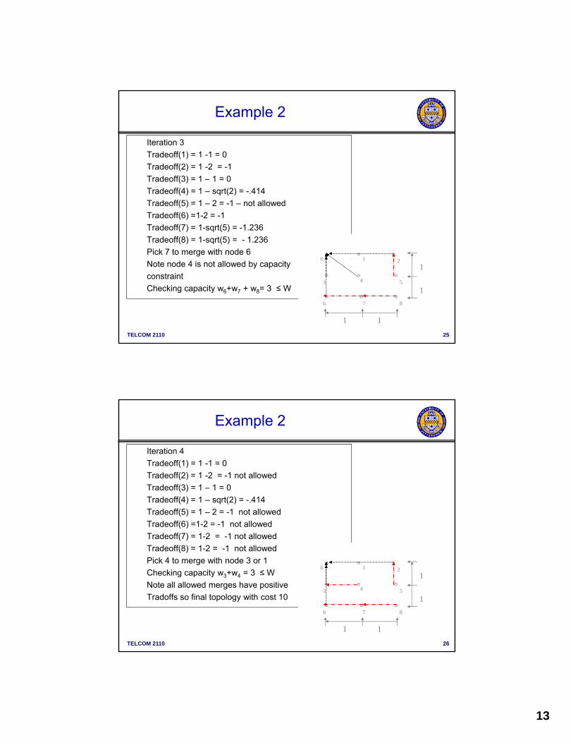
Example 2
Iteration 3
Tradeoff(1) = 1 -1 = 0
Tradeoff(2) = 1 -2 = -1
Tradeoff(3) = 1 – 1 = 0
Tradeoff(4) = 1 – sqrt(2) = -.414
Tradeoff(5) = 1 – 2 = -1 – not allowed
Tradeoff(6) =1-2 = -1
Tradeoff(7) = 1-sqrt(5) = -1.236
Tradeoff(8) = 1-sqrt(5) = - 1.236
Pick 7 to merge with node 620 1
TELCOM 2110 25
Note node 4 is not allowed by capacity
constraint
Checking capacity w6+w7 + w8= 3 ≤ W
20
3 4
6
5
1
7 8
1
1
1
1
Example 2
Iteration 4
Tradeoff(1) = 1 -1 = 0
Tradeoff(2) = 1 -2 = -1 not allowed
Tradeoff(3) = 1 – 1 = 0
Tradeoff(4) = 1 – sqrt(2) = -.414
Tradeoff(5) = 1 – 2 = -1 not allowed
Tradeoff(6) =1-2 = -1 not allowed
Tradeoff(7) = 1-2 = -1 not allowed
Tradeoff(8) = 1-2 = -1 not allowed
Pick 4 to merge with node 3 or 120 1
TELCOM 2110 26
Checking capacity w3+w4 = 3 ≤ W
Note all allowed merges have positive
Tradoffs so final topology with cost 10
20
3 4
6
5
1
7 8
1
1
1
1

14
Esau-Williams Algorithm
• Remember E-W algorithm is a heuristic not minimum cost design
• Numerical results indicate it usually provides better solution then SPT, MST, and Prim-Dijkstra
• Known drawback is line crossing (20 node example)
TELCOM 2110 27
Sharma’s Algorithm
• Heuristic algorithm to create networks with no lines crossingUseful when physical constraints (duct for running cable) dictate that no lines cross
1. Compute the angle s from each site S to the central site C. If S and C have the same coordinate, set s = 0.
2. Sort the angles s from smallest to largest3. Beginning at a site Sfirst, create a set of nodes clockwise (or
counterclockwise) from Sfirst. A set is complete when adding the next node would put setw(site) > W. The next set starts with that node.
4. The design is completed by building a MST on each set with the addition of the central node C
TELCOM 2110 28
addition of the central node C.Comment
If the angles s are distinct, then if the cost function is a linear or piecewise linear metric, Sharma’s algorithm builds CMSTs without crossings provided that all the central angles are less than π.

15
• Consider the grid network below. – This network can occur in a cellular network in a downtown urban
environment Where the nodes represent base stations and the
Example of Sharma’s algorithm
environment. Where the nodes represent base stations and the hub/central node a base station controller
– For the example Node 0 is the central node.
– The weight of each individual node is 1, except for nodes 4 and 5, which have a weight of 2. The cost function C(i,,j) is given by the physical distance between nodes i and j. W=3
TELCOM 2110 29
20
3 4
6
5
1
7 8
1
1
1
1
Angle of each node
1 = 0,
2 = 0
Example of Sharma’s algorithm
2 0
3 = -90
4 = -45
5 = -22.5
6 = -90
7 = -72.5
8 = -4520 1
TELCOM 2110 30
Sorted angles
{1 2 5 4 8 7 3 6 }
20
3 4
6
5
1
7 8
1
1
1
1
16
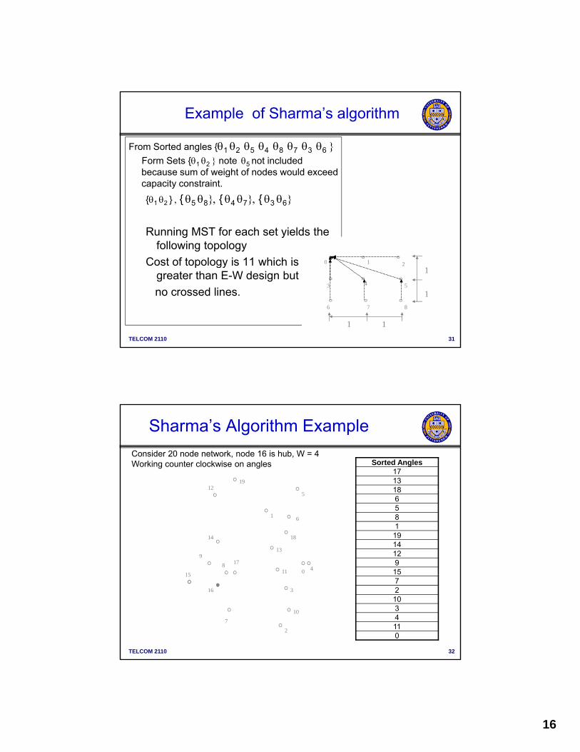
From Sorted angles {1 2 5 4 8 7 3 6 Form Sets {1 2 note 5 not included because sum of weight of nodes would exceed
Example of Sharma’s algorithm
gcapacity constraint.
{1 2 } { 5 8{ 4 7{ 3 6
Running MST for each set yields the following topology
Cost of topology is 11 which is 20 1
TELCOM 2110 31
Cost of topology is 11 which is greater than E-W design but
no crossed lines.
20
3 4
6
5
1
7 8
1
1
1
1
Sharma’s Algorithm Example
1912
Sorted Angles171318
Consider 20 node network, node 16 is hub, W = 4Working counter clockwise on angles
4011
6
18
13
5
1
12
14
9
15
8 17
186581
1914129
15
TELCOM 2110 32
2
10
3
15
7
16
72
1034110

17
Sharma’s Algorithm Design
• Cost= $16021, Sfirst = N17
TELCOM 2110 33
Sharma vs. Esau-Williams
• EW_Ratio=SharmaCost/EWCost; S_Ratio=EWCost/SharmaCost
In general use Esau Williams unless require no lines cross• In general use Esau- Williams unless require no lines cross
TELCOM 2110 34
18
Access Design Problems
• Can roughly categorize access design problems
One speed one center designIBM VLR
HLR
AUC EIR
– One speed one center design• Capacitated MST problem
– Esau-Williams algorithm– Sharma algorithm
• Examples – Local loop in telephone network
– Multi-speed access design
MSC
BS7BS5
BS2
BS3
BS4
BS1
SD
Centillion 1400Bay Networks
ETHER RS 232C
PC CARD
P*8x50OOO130A O N6
INS ACT ALMRST LINK
PWR ALM FAN0FAN1PWR0PWR1
ALM
BSC
BS2
BS3
BS4
BS1
SD
Centillion 1400Bay Networks
ETHER RS 232C
PC CARD
P* 8x50OOO130A O N6
INS ACT ALMRST LINK
PWR ALM FAN0FAN1 PWR0PWR1
ALM
BSC
SD
Centillion 1400Bay Networks
ETHER RS 232C
PC CARD
P* 8x50OOO130A O N6
INS ACT ALMRST LI NK
PWR ALM FAN0 FAN1PWR0 PWR1
ALM
BSC
TELCOM 2110 35
• Have multiple link speeds/types– For example, LAN design from variety of
hosts
– Multi-center Design• Cellular networks with multiple base
station controllers
BS5
BS6BS7
BS5
BS6
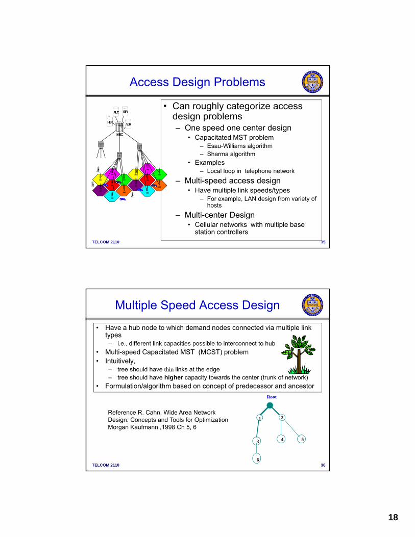
Multiple Speed Access Design
• Have a hub node to which demand nodes connected via multiple link types – i.e., different link capacities possible to interconnect to hub
C S ( CS )• Multi-speed Capacitated MST (MCST) problem• Intuitively,
– tree should have thin links at the edge– tree should have higher capacity towards the center (trunk of network)
• Formulation/algorithm based on concept of predecessor and ancestor
Root
R f R C h Wid A N t k
TELCOM 2110 36
21
3 4 5
6
Reference R. Cahn, Wide Area NetworkDesign: Concepts and Tools for OptimizationMorgan Kaufmann ,1998 Ch 5, 6

19
Multiple Speed Access Design
• Formulation/algorithm based on concept of predecessor and ancestor• A tree T rooted at a node Root can be represented uniquely by a
predecessor function predThe function pred( ) gives the node one hop closer to the root from the– The function pred( ) gives the node one hop closer to the root from the node in question
– pred(6) = 3, pred(3) = 1, pred(1) = root, pred(4) = 2, etc.– pred2(6) = pred(pred(6)) = 1, pred3(6) = root
• Define pred(root) = root• Given a tree T and the associated predecessor function, the ancestors
of N are all the nodes N’ that are downstream from the node away from the root node.
Ancestor(1) = {3,6}Root
TELCOM 2110 37
( ) { , }Ancestor(2) = {4,5}Ancestor(3) = {6}
(bit of a misnomer !)
pred n (N’) = N for some n > 0
21
3 4 5
6
Multispeed CMST Problem
• Given – set of nodes N0, N1, N2, … , Nn.
set of weights (traffic demand) w w w for each node– set of weights (traffic demand) w1, w2, … , wn for each node
– set of link types L1, L2, … , Lm
– Set of capacities W1, W2, … , Wm
– cost matrix C(i, j, k) that gives the cost of a link of type Lk between Ni
and Nj
• Find: the tree rooted at N0 and the link assignments such that(i) lC )(
TELCOM 2110 38
(i)
(ii)
Linksl
ljiCMinimize ),,(
)(
))(,()(NAncestorsNi
NpredNLinki Ww

20
Multiple Speed CMST Problem
• Consider Multi-speed capacitated MST problem constraint
))(,()( NpredNLinki Ww
• Capacity of upstream link can carry demand of downstream nodes
0
Root
)(NAncestorsNi
For example link(2,0)w2 + w4 + w5 < W(2 0)
TELCOM 2110 39
21
3 4 5
6
w2 w4 w5 W(2,0)
For link(1,0)w1 + w3 + w6 < W(1,0)
Objective is the minimize link cost while meeting demand requirements.
Cahn’s Multi-speed Local Access Algorithm
• Heuristic Algorithm to solve mCMST similar to Esau-Williams1. Assign each node n the smallest link capacity Wl possible to directly
connect it to the root. 2 For each node n compute2. For each node n, compute
spare_capacity(n)=Wl -wn set pred(n)=0 where 0 denotes root3. Calculate tradeoffs for each node n
– Tradeoffn(i) is savings from linking node n to node i rather than linking directly to the root node 0.
Tradeoffn(i)= C(n,i, l) + Upgrade(i,wn) – C(n,0, l )– May have to upgrade links to carry additional traffic
• Need to add un= max(0, wn - spare_capacity(i)) bandwidth • Upgrade(i, un) function determines the cost of adding un units to the links that
connect i and 0
TELCOM 2110 40
connect i and 0. – Tradeoff of a node n is the minimum of all tradeoffs
Tradeoff(n)= mini (Tradeoffn(i))
4. Modify tree (add link to relay node/remove direct link to root) for node with minimum tradeoff among all nodes
5. Repeat 3 until all tradeoff values positive

21
Consider network with four access nodes to connect to a hub want a MAXIMUM link utilization of 50%
MSLA Example
Node Weight (kbps) Link Type CapacityNode Weight (kbps)
1 20,000
2 2,400
3 9,600
4 4,800
Link Type Capacity
0 9.6 Kbps
1 56 Kbps
2 64 Kbps
Link cost are a piecewise linear function of distance and data rate
TELCOM 2110 41
Link cost are a piecewise linear function of distance and data rate
MLSA Example
Link Cost Matrices for each link type
• Link Costs
TELCOM 2110 42

22
• Step 1 Connect each node directly to root with minimum link capacity that meets design objective (i e 50% link
MSLA Example
objective (i.e. 50% link utilization or less)
• Initial Cost = 10+7+10+7 = 34• Step 2 Calculate Spare Capacity
on each link (Max Utilization=0.5)
spare_capacity(1)=0.5*56000-20000=8000
L1
L0
L0
TELCOM 2110 43
spare_capacity(2)=0.5*9600-2400=2400
spare_capacity(3)=0.5*56000-9600=18400
spare_capacity(4)=0.5*9600-4800=0
L1
• Step 3 Calculate Tradeoffs for each node
Tradeoff (i)= C(n i l) +
MSLA Example
Tradeoffn(i)= C(n,i, l) + Upgrade(i,wn) – C(n,0, l )
Example node 1Tradeoff1(2)= C(1,2, l) +
Upgrade(2,20000) – C(1,0, 1 )
= 10 + (15-7) -10 = 8
Tradeoff1(3)= C(1,3, l) + U d (3 20000) C(1 0 1 )
L1
L0
L0
TELCOM 2110 44
Upgrade(3,20000) – C(1,0, 1 )
= 12 + (20-10) -10 = 12
Tradeoff1(4)= C(1,4, l) + Upgrade(4,20000) – C(1,0, 1 )
= 12 + (15 -7) -10 = 10
Tradeoff(1) = min{8,12,10} = 8
L1

23
• Step 3 Calculate Tradeoffs for each node
F d 2
MSLA Example
For node 2Tradeoff2(1)= C(2,1, l) +
Upgrade(1,2400) – C(2,0, 1 )
= 7 + 0 - 7 = 0
Tradeoff2(3)= C(2,3, l) + Upgrade(3,2400) – C(2,0, 1 )
= 5 + 0 -7 = -2
d ff ( ) C(2 l)
L1
L0
L0
TELCOM 2110 45
Tradeoff2(4)= C(2,4, l) + Upgrade(4,2400) – C(2,0, 1 )
= 6 + (15 -7) -7 = 7
Tradeoff(2) = min{0,-2,7} = -2
L1
• Step 3 Calculate Tradeoffs for each node
F d 3
MSLA Example
For node 3Tradeoff3(1)= C(3,1, l) +
Upgrade(1,9600) – C(3,0, 1 )
= 12 + (20-10) - 10= 12
Tradeoff3(2)= C(3,2, l) + Upgrade(2,9600) – C(3,0, 1 )
= 12 + (15-7) -10= 10
d ff ( ) C(3 l)
L1
L0
L0
TELCOM 2110 46
Tradeoff3(4)= C(3,4, l) + Upgrade(4,9600) – C(3,0, 1 )
= 10 + (15 -7) -10 = 8
Tradeoff(3) = min{12,10,8} = 8
L1

24
• Step 3 Calculate Tradeoffs for each node
For node 4
MSLA Example
Tradeoff4(1)= C(4,1, l) + Upgrade(1,4800) –C(4,0, 1 )
= 6 + 0 - 7 = -1
Tradeoff4(2)= C(4,2, l) + Upgrade(2,4800) –C(4,0, 1 )
= 6 + (15-7) -7 = 7
Tradeoff4(3)= C(4,3, l) + Upgrade(3,4800) –C(4,0, 1 )
L1
L0
L0
TELCOM 2110 47
( )
= 5 + 0 -7 = -2
Tradeoff(4) = min{-1,7,-2} = -2
Comparing the tradeoff values of all four nodes Tradeoff (4)=Tradeoff(2) = -2 arbitrarily pick Node 4
L1
MSLA Example
Step 4 remove link from 4 to 0And add link from 4 to 3 which is I ’ l d ff l d
Iteration 2: Note adjust node weightsL1
L1
L0
L0
Iteration 1 It’s lowest tradeoff value node
Iteration 1 topology
TELCOM 2110 48
Repeat tradeoff calculations
Result is Let N4 goes through N3,no upgrade is needed and it is the best tradeoff value
Iteration 2 topology
L0L0
L1
L1
Iteration 2

25
L0L0
Iteration 2
MSLA Example
• Iteration 3 results in connecting N3 to N1 and increase (1,0) to 256 Kbps link.
• All tradeoff values are positive - STOP
L1
L1
L0L0
L1
Final design
TELCOM 2110 49
L2
Larger Example of MSLA Algorithm:
We have 20 nodes in and the weights of the nodes are generated according to the above TABLE TRAFDIST.
Weights of nodes are shown in the TABLE SITES. Note that the weight of N0 is normalized so that it sums to the traffic from all the other sites.
To simplify the mathematics we
TELCOM 2110 50
To simplify the mathematics, we assume that every line can be used to 100% of capacity.

26
Esau Williams: 20 nodes with 9.6Kbps links
TELCOM 2110 51
Cost = $26,963
Only 9 sites share links to N0, more like a star.
Esau Williams: 20 nodes with 56Kbps links
TELCOM 2110 52
Cost = $30,160
A nice tree structure, but the cost is higher because out on the periphery of the network there is too much capacity.

27
MSLA: 20 nodes with multispeed links
TELCOM 2110 53
Cost = $22,760
There is a central D56 tree and a peripheral D96 tree
Access Design Problems
• Can roughly categorize access design problems IBM VLR
HLR
AUC EIR
g p– One speed one center design
• Capacitated MST problem– Esau-Williams algorithm
– Sharma algorithm
– Multi-speed access design
MSC
BS7BS5
BS2
BS3
BS4
BS1
SD
Centillion 1400Bay Networks
ETHER RS 232C
PC CARD
P*8x50OOO130A O N6
INS ACT ALMRST LINK
PWR ALM FAN0FAN1PWR0PWR1
ALM
BSC
BS2
BS3
BS4
BS1
SD
Centillion 1400Bay Networks
ETHER RS 232C
PC CARD
P* 8x50OOO130A O N6
INS ACT ALMRST LINK
PWR ALM FAN0FAN1 PWR0PWR1
ALM
BSC
SD
Centillion 1400Bay Networks
ETHER RS 232C
PC CARD
P* 8x50OOO130A O N6
INS ACT ALMRST LI NK
PWR ALM FAN0 FAN1PWR0 PWR1
ALM
BSC
TELCOM 2110 54
• mCMST – MSLA
– Multi-center Design• Multiple Centers (hubs) – nodes
can connect to any center
BS5
BS6BS7
BS5
BS6

28
MultiCenter Access Design
• Given– A set B of hub or backbone sites {B0, …, Bm}
A set N of access nodes {N N }– A set N of access nodes {N1, … , Nn}
• A set of weights {w1, … , wn} for each access node
• A upper limit on capacity, W (one speed design).
• A cost matrix Cost(i,j) giving the costs between each (hub)
backbone/access pair of sites.
• Build a set of trees that connect each access node to a hub
TELCOM 2110 55
Build a set of trees that connect each access node to a hub
• Constructing a forest of trees – often not interconnected
• The multicenter local – access problem is to find a set of trees T1, … , Tk such that
MultiCenter Local Access Problem (MCLA)
(1) Exactly 1 backbone site belongs to each tree
(2) The link capacity is not violated
WwTN i
TELCOM 2110 56
(3) The Cost is minimum
jiTN i
Trees Linksl ll NodeNodeC )2,1(

29
Example
Consider site with 3 backbone nodes
Circles : X, Y and Z
Have 17 access nodes
Squares: A, B, C and D, etc
Could represent host and Ethernet switches connected to campus backbone
TELCOM 2110 57
• This problem is a much more complex than the single-center oneS h d h i i i
MultiCenter Local Access Problem
• Suppose we have n access nodes that we want to partition into sets of M nodes (i.e., one set for each backbone node. The number of possible partitions is :
Af i i i f h i l M
n
M
Mn
M
n2 Even for the modest number n = 21, M = 7
the complexity is daunting .
TELCOM 2110 58
• After partitioning of the access sites must solve M capacitated MST problems (use Esau-Williams algorithm or Sharma algorithm)
• How to partition into sets?

30
Nearest-Neighbor Esau-Williams (NNEW)
• For each b in B, let Sb={ nN | Cost(n,b) < Cost(n,b’) b’B}Group nodes in to sets based on nearest backbone node as judged by the direct connection costdirect connection cost
• If n is equidistant between several backbone nodes, add n to one Sb at random.
• Use Esau-Williams to construct a capacitated MST on each set bSb.
Example: A belongs to X set of nodes (since X is the closest backbone node to A)
TELCOM 2110 59
B to YD to ZC is equidistant to X and Z so can be placed in either set.
Nearest-Neighbor Esau-Williams (NNEW)
• Assume topology at right
• B = {9,10,11}
• N = {0,1,2,3,4,5,6,7,8}
• Weight of each node is 1, except for nodes 4 and 5, which have weight 2
• Cost C(i,j) is given by the physical distance between nodes i and j
TELCOM 2110 60
• Capacity of link W = 3
• Step 1 is partition nodes into 3 sets using nearest-neighbor algorithm

31
Nearest-Neighbor Esau-Williams (NNEW)
• Use Esau-Williams to construct a capacitated MST on each set Sb
• Backbone nodes connected separately
TELCOM 2110 61
Test of Quality of Design
• Test: reattach the leaves to a different tree and see if it reduces the cost.
• The quality of NNEW is not that great
TELCOM 2110 62

32
• NNEW algorithm doesn’t always work well
• Problem is the location of the other access nodes cannot be ignored when deciding which access nodes should home to which center.
( ) f
Nearest-Neighbor Esau-Williams (NNEW)
• Example two hubs (N1, N2), cheaper design if N5 connects through N9 to N2 - but nearest neighbor prohibits this.
TELCOM 2110 63
MultiCenter Esau-Williams (MCEW)
• Recall that, in Esau-Williams algorithm – Calculate the tradeoff as the saving by linking Ni to Nj instead of linking
it directly to the center/root.
T d ff(N ) i C (N N ) C (C (N ) C )Tradeoff(Ni) = minjCost(Ni, Nj) - Cost(Comp(Ni),Center)
• MCEW algorithm replaces the tradeoff function with:
Tradeoff(Ni) = minjCost(Ni, Nj) - Cost(Comp(Ni),Center(Ni))
• Initially, we set Center(Ni) to be the closest backbone center.If d N i d i h d N d
TELCOM 2110 64
• If node Ni is merged with node Nj, update Center(Ni)=Center(Nj).
• MCEW has an advantage over NNEW when size of nodes in clusters large

33
NNEW vs. MCEW
• Test of quality show MCEW has better solution
TELCOM 2110 65
Access Design Problems
• Looked at three access design problems – One speed one center designp g
• Capacitated MST problem– Esau-Williams algorithm– Sharma algorithm
– Multi-speed access design• mCMST – MSLA
– Multi-center Design• NNEW, MCEW
S l ti l ith t t
TELCOM 2110 66
• Solution algorithms not cast in stone – often need to add constraints to improve design or make practical
34
Some Branches Have Too Many Nodes.
• EW tests only if the combined weight of the two components doesn’t exceed the upper bound weight limitbound weight_limit.
• May have too many nodes in a component (e.g. collision domain in LAN grows with number of nodes)
• Solution: add additional size_limit constraints that prohibit the merge of two
m ts ith t m
TELCOM 2110 67
components with too many nodes.
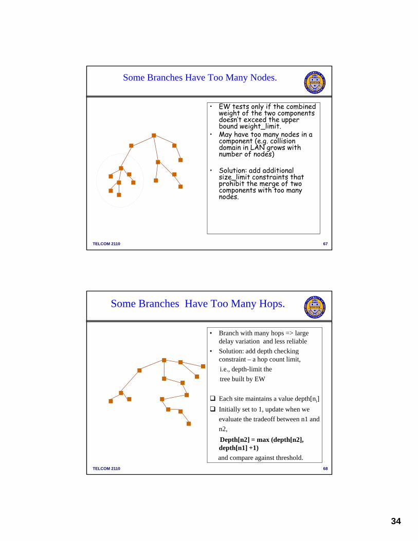
Some Branches Have Too Many Hops.
• Branch with many hops => large delay variation and less reliable
• Solution: add depth checkingSolution: add depth checking constraint – a hop count limit,
i.e., depth-limit the
tree built by EW
Each site maintains a value depth[ni]
Initially set to 1, update when we
TELCOM 2110 68
evaluate the tradeoff between n1 and
n2,
Depth[n2] = max (depth[n2], depth[n1] +1)
and compare against threshold.

35
Some Node in Tree Has Too Many Links
Degree of node directly relates to port count, may want to keep port countwant to keep port count below a given value
• Solution: add degree constraint
Initialize the degree of each site to 1, when we accept the merge from n1
TELCOM 2110 69
p gto n2 then we increase the degree of n2 by 1. Do not accept merges that violates the constraint.
Access Design Problems
• Looked at three access design problems – One speed one center design– Multi-speed access design
Multi center Design– Multi-center Design
• Studied algorithms for each case• Algorithms are incorporated in software tools
– freeware DELITE tool (see class web page) – VPISystems OnePlan Access tool
TELCOM 2110 70