Embed Size (px)
Citation preview
NETWORK ANALYSIS Duygu Tosun-Turgut, Ph.D. Center for Imaging of Neurodegenerative Diseases Department of Radiology and Biomedical Imaging [email protected]
What is a network? - Complex web-like structures
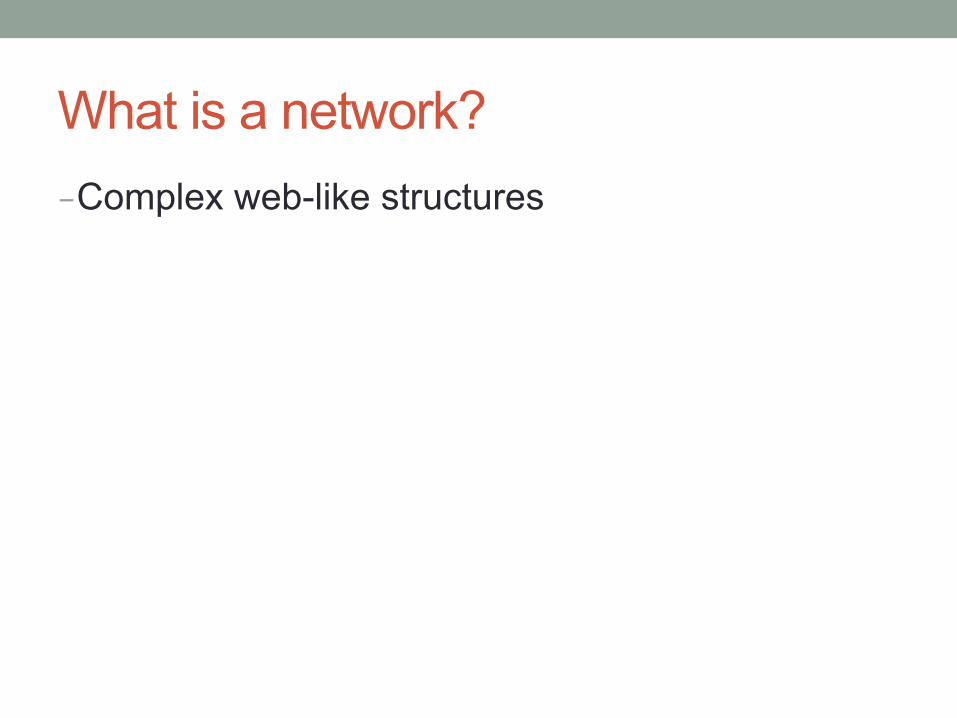
Internet … is network of routers and computers linked by physical or wireless links
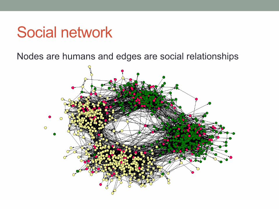
Social network Nodes are humans and edges are social relationships
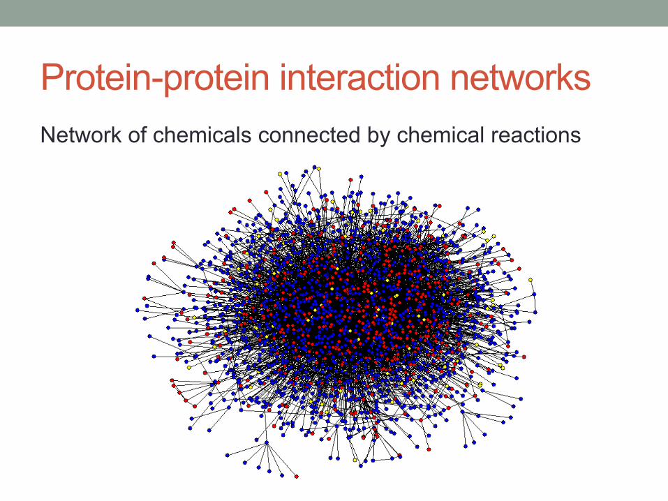
Protein-protein interaction networks Network of chemicals connected by chemical reactions
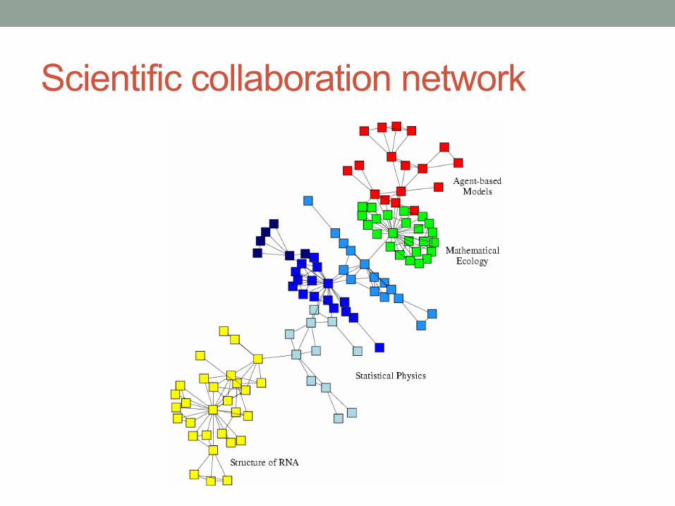
Scientific collaboration network
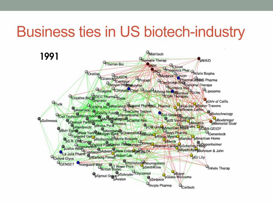
Business ties in US biotech-industry
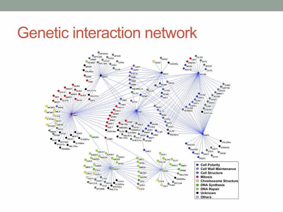
Genetic interaction network
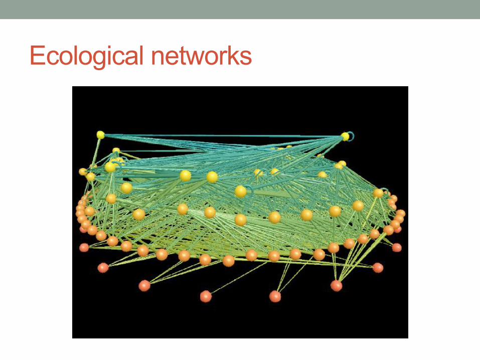
Ecological networks
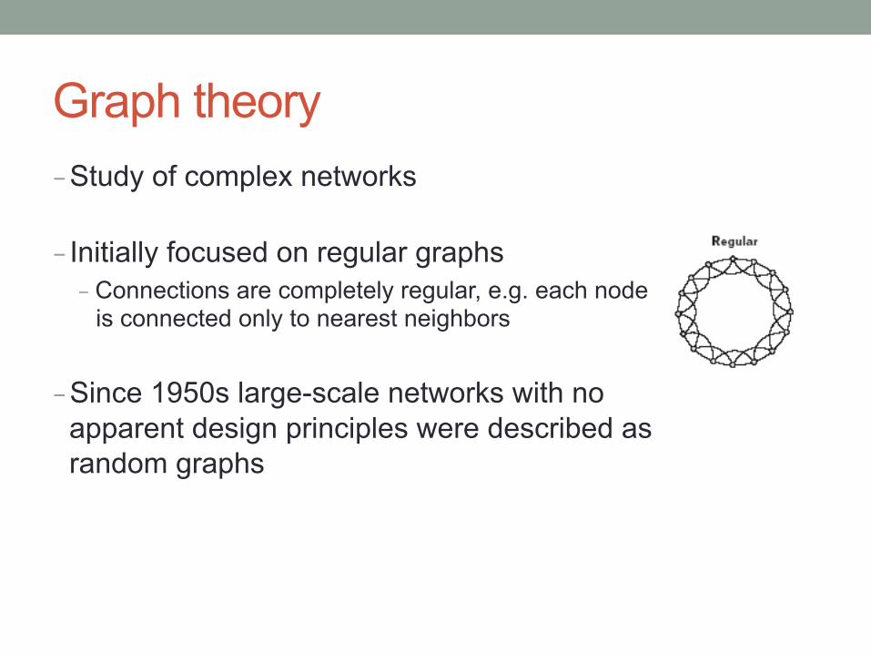
Graph theory - Study of complex networks
- Initially focused on regular graphs - Connections are completely regular, e.g. each node
is connected only to nearest neighbors
- Since 1950s large-scale networks with no apparent design principles were described as random graphs
What makes a problem graph-like? - There are two components to a graph - Nodes and edges
- In graph-like problems, these components have natural correspondences to problem elements - Entities are nodes and interactions between entities are edges
- Most complex systems are graph-like
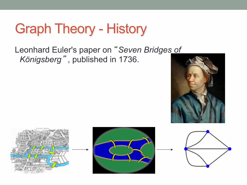
Graph Theory - History Leonhard Euler's paper on “Seven Bridges of
Königsberg” , published in 1736.
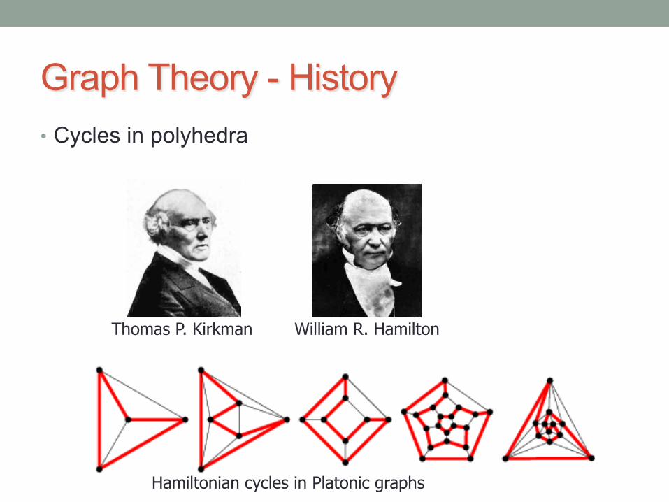
Thomas P. Kirkman William R. Hamilton
Hamiltonian cycles in Platonic graphs
Graph Theory - History • Cycles in polyhedra
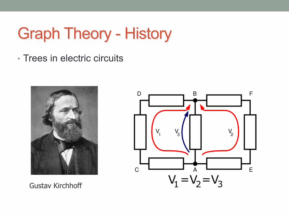
Graph Theory - History • Trees in electric circuits
Gustav Kirchhoff
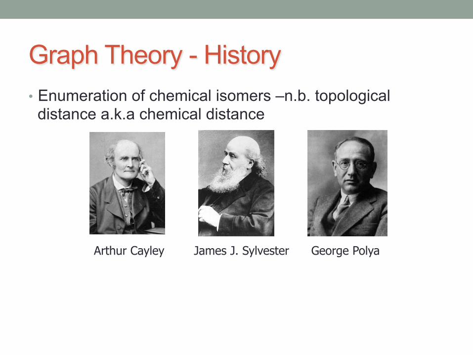
Graph Theory - History • Enumeration of chemical isomers –n.b. topological
distance a.k.a chemical distance
Arthur Cayley James J. Sylvester George Polya
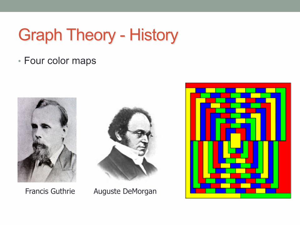
Graph Theory - History • Four color maps
Francis Guthrie Auguste DeMorgan
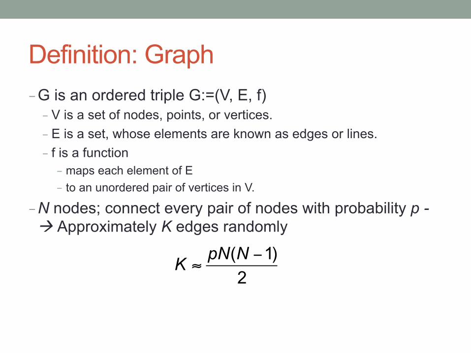
Definition: Graph - G is an ordered triple G:=(V, E, f) - V is a set of nodes, points, or vertices. - E is a set, whose elements are known as edges or lines. - f is a function - maps each element of E - to an unordered pair of vertices in V.
- N nodes; connect every pair of nodes with probability p -à Approximately K edges randomly
( 1)2
pN NK −≈
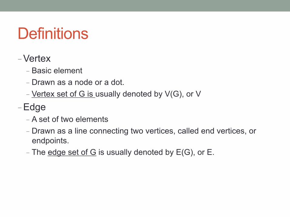
Definitions - Vertex - Basic element - Drawn as a node or a dot. - Vertex set of G is usually denoted by V(G), or V
- Edge - A set of two elements - Drawn as a line connecting two vertices, called end vertices, or
endpoints. - The edge set of G is usually denoted by E(G), or E.
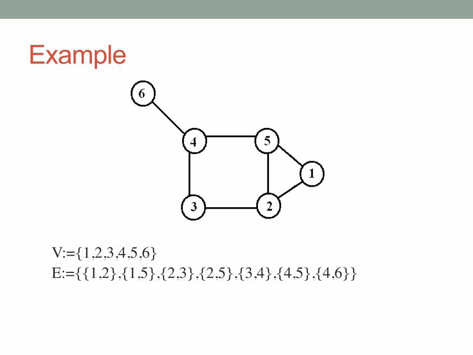
Example
V:={1,2,3,4,5,6} E:={{1,2},{1,5},{2,3},{2,5},{3,4},{4,5},{4,6}}
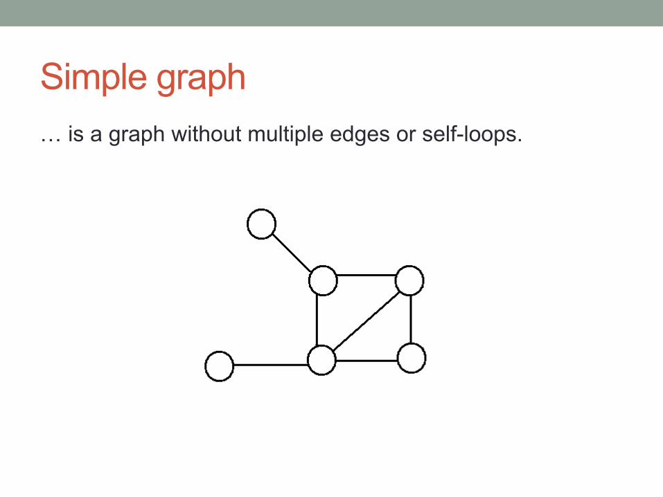
Simple graph … is a graph without multiple edges or self-loops.
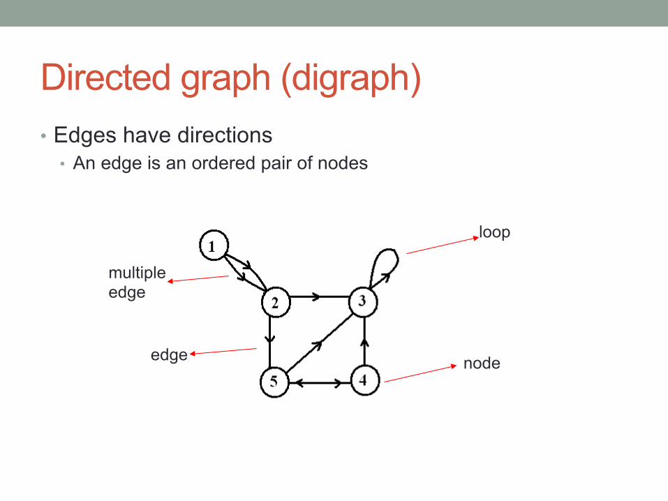
Directed graph (digraph) • Edges have directions
• An edge is an ordered pair of nodes
loop
node
multiple edge
edge
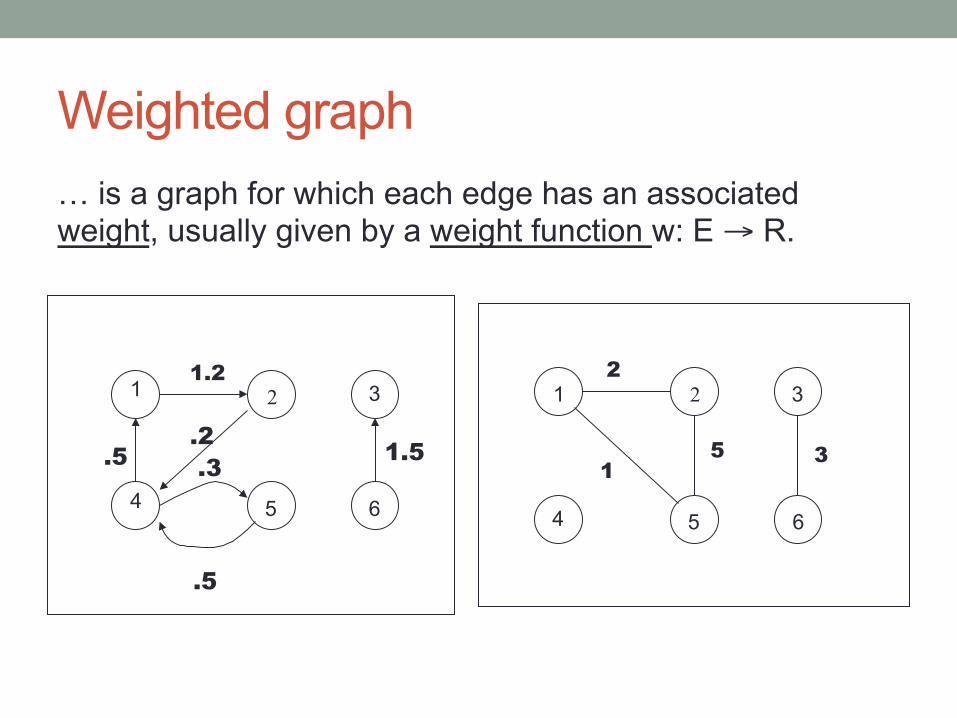
Weighted graph … is a graph for which each edge has an associated weight, usually given by a weight function w: E → R.
1 2 3
4 5 6
.5
1.2
.2
.5
1.5 .3
1
4 5 6
2 3 2
1 3 5
Structures and structural metrics - Graph structures are used to isolate interesting or
important sections of a graph - Interesting because they form a significant domain-specific
structure, or because they significantly contribute to graph properties
- A subset of the nodes and edges in a graph that possess certain characteristics, or relate to each other in particular ways
- Structural metrics provide a measurement of a structural property of a graph - Global metrics refer to a whole graph - Local metrics refer to a single node in a graph
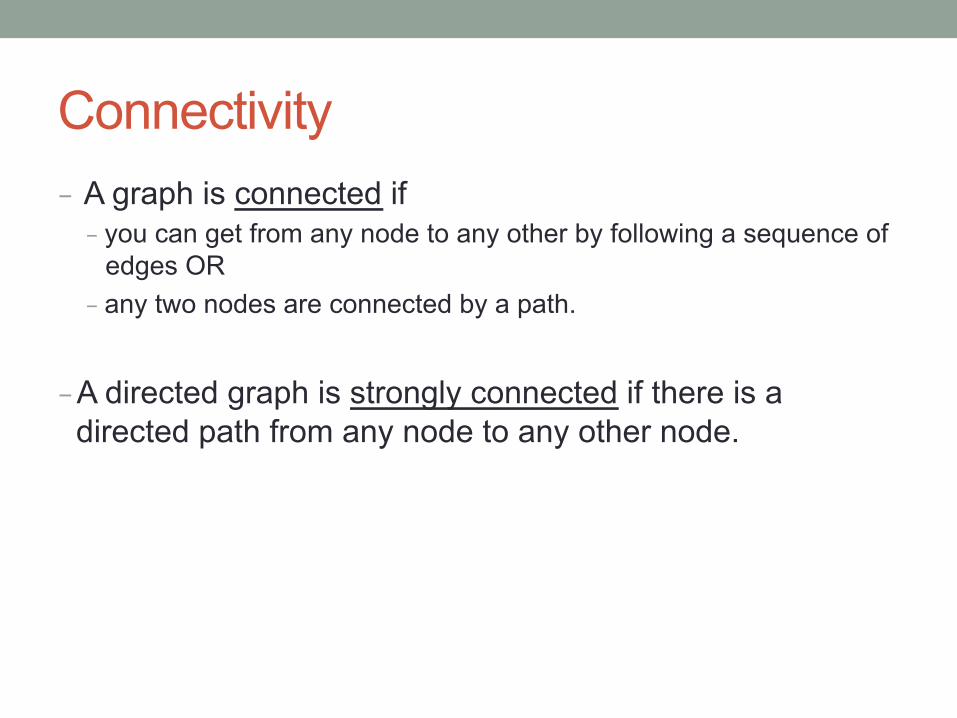
Connectivity - A graph is connected if - you can get from any node to any other by following a sequence of
edges OR - any two nodes are connected by a path.
- A directed graph is strongly connected if there is a directed path from any node to any other node.
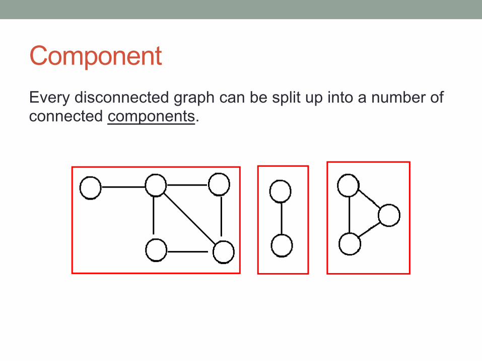
Component Every disconnected graph can be split up into a number of connected components.
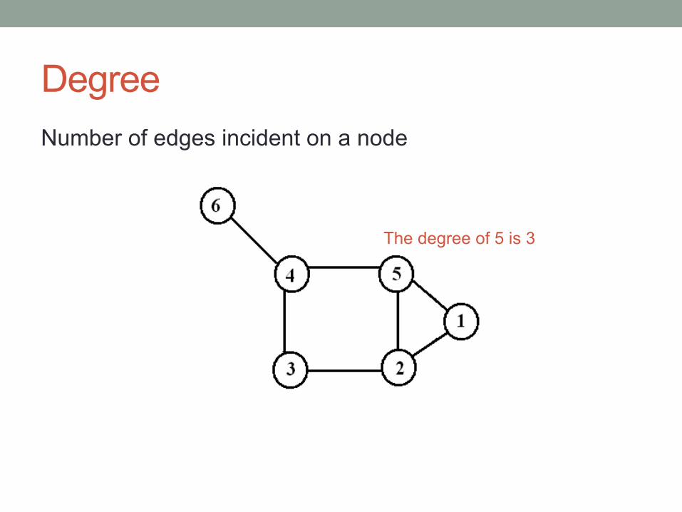
Degree Number of edges incident on a node
The degree of 5 is 3
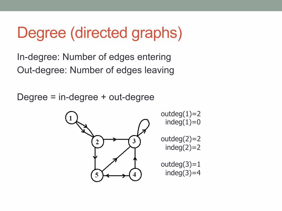
Degree (directed graphs) In-degree: Number of edges entering Out-degree: Number of edges leaving
Degree = in-degree + out-degree
outdeg(1)=2 indeg(1)=0 outdeg(2)=2 indeg(2)=2 outdeg(3)=1 indeg(3)=4
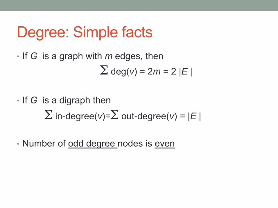
Degree: Simple facts • If G is a graph with m edges, then
Σ deg(v) = 2m = 2 |E |
• If G is a digraph then
Σ in-degree(v)=Σ out-degree(v) = |E |
• Number of odd degree nodes is even
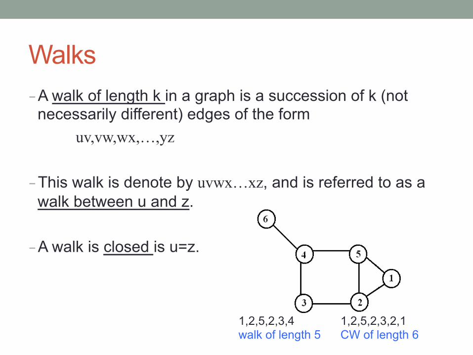
Walks - A walk of length k in a graph is a succession of k (not
necessarily different) edges of the form uv,vw,wx,…,yz
- This walk is denote by uvwx…xz, and is referred to as a
walk between u and z.
- A walk is closed is u=z.
1,2,5,2,3,4 1,2,5,2,3,2,1 walk of length 5 CW of length 6
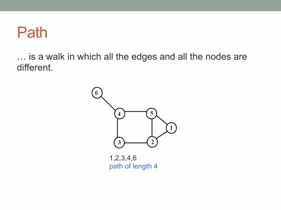
Path … is a walk in which all the edges and all the nodes are different.
1,2,3,4,6 path of length 4
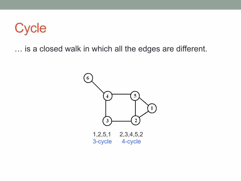
Cycle … is a closed walk in which all the edges are different.
1,2,5,1 2,3,4,5,2 3-cycle 4-cycle
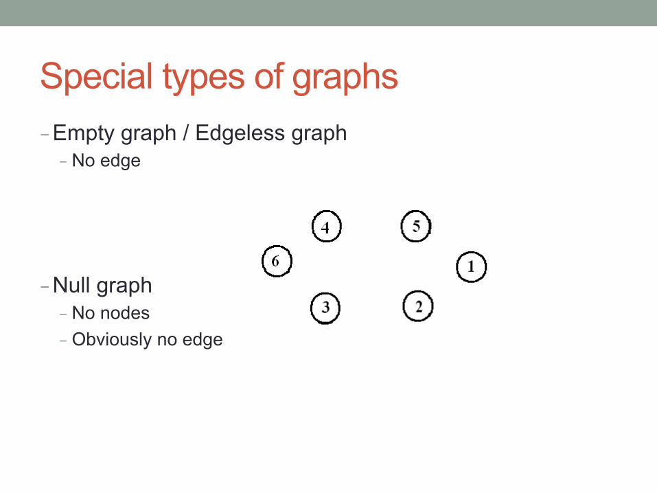
Special types of graphs - Empty graph / Edgeless graph - No edge
- Null graph - No nodes - Obviously no edge
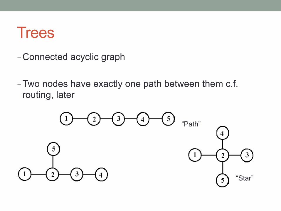
Trees - Connected acyclic graph
- Two nodes have exactly one path between them c.f. routing, later
“Path”
“Star”
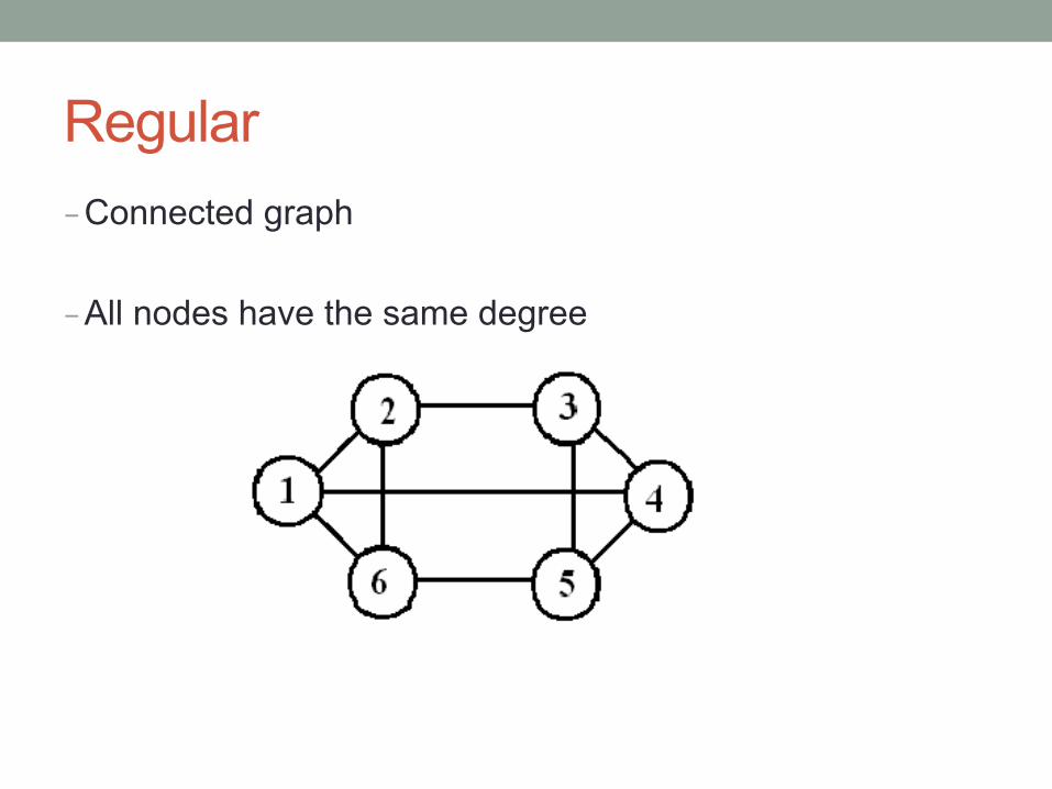
Regular - Connected graph
- All nodes have the same degree
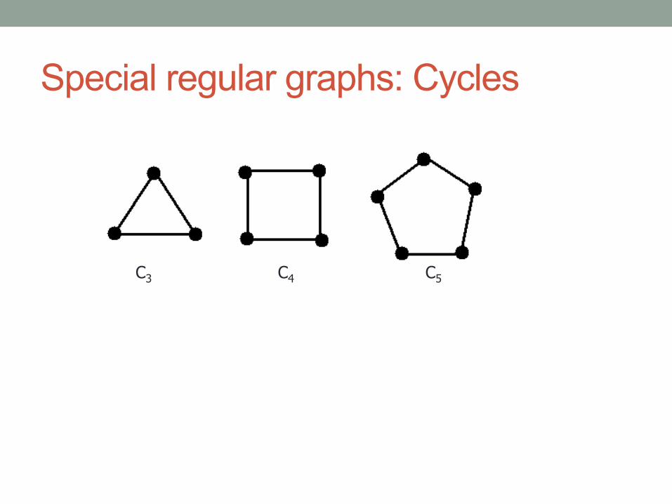
Special regular graphs: Cycles
C3 C4 C5
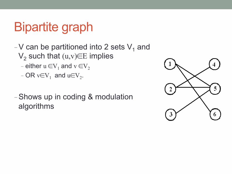
Bipartite graph - V can be partitioned into 2 sets V1 and
V2 such that (u,v)∈E implies - either u ∈V1 and v ∈V2
- OR v∈V1 and u∈V2.
- Shows up in coding & modulation algorithms


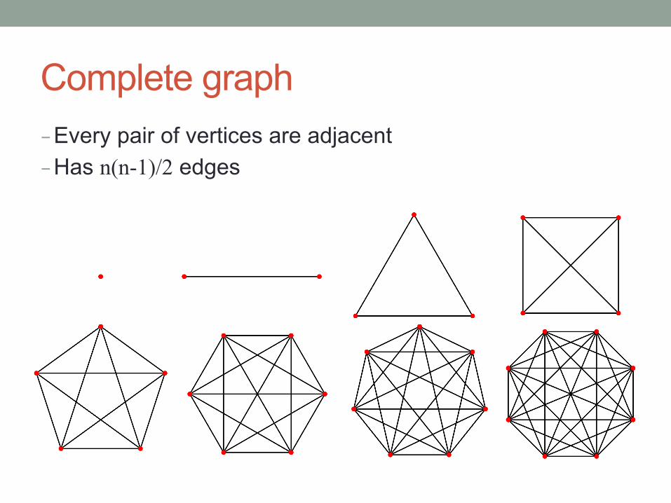
Complete graph - Every pair of vertices are adjacent - Has n(n-1)/2 edges
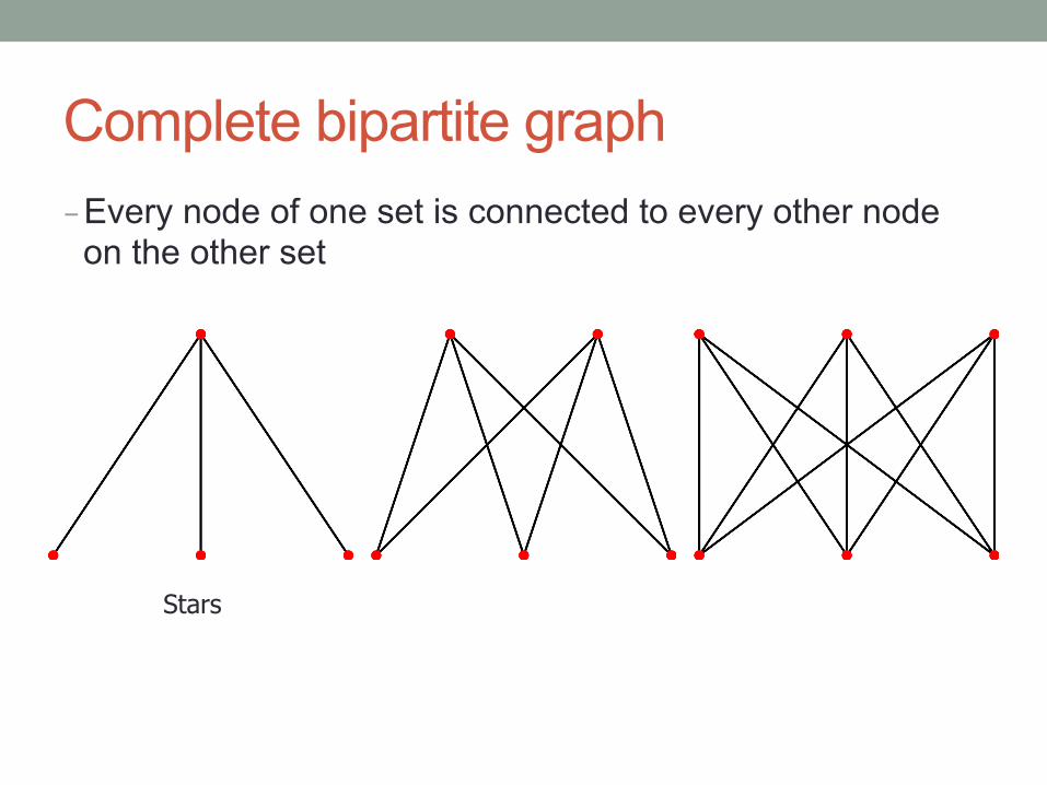
Complete bipartite graph - Every node of one set is connected to every other node
on the other set
Stars
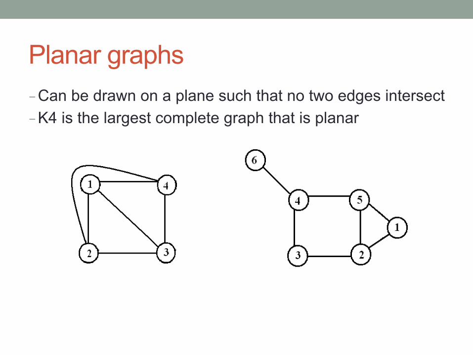
Planar graphs - Can be drawn on a plane such that no two edges intersect - K4 is the largest complete graph that is planar
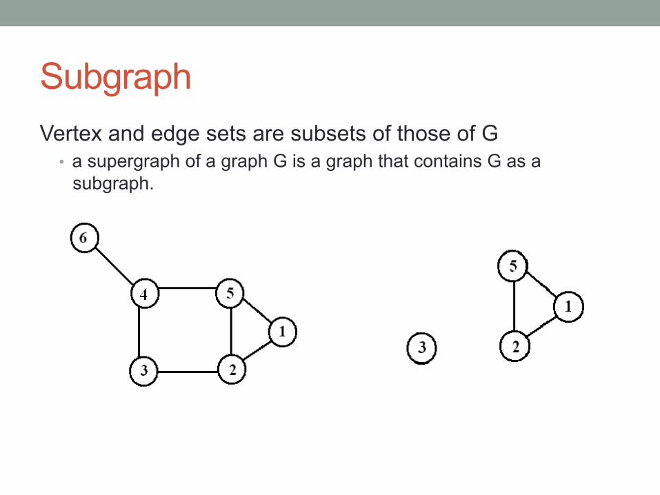
Subgraph Vertex and edge sets are subsets of those of G
• a supergraph of a graph G is a graph that contains G as a subgraph.
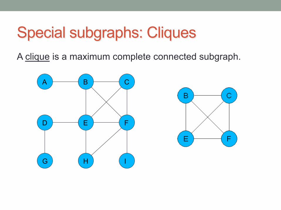
Special subgraphs: Cliques A clique is a maximum complete connected subgraph.
A B
D
H
F E
C
I G
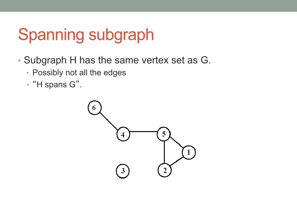
Spanning subgraph • Subgraph H has the same vertex set as G.
• Possibly not all the edges • “H spans G”.
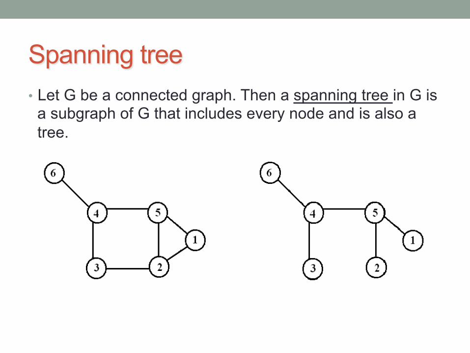
Spanning tree • Let G be a connected graph. Then a spanning tree in G is
a subgraph of G that includes every node and is also a tree.
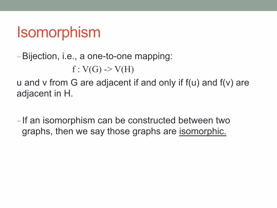
Isomorphism - Bijection, i.e., a one-to-one mapping:
f : V(G) -> V(H) u and v from G are adjacent if and only if f(u) and f(v) are adjacent in H.
- If an isomorphism can be constructed between two graphs, then we say those graphs are isomorphic.
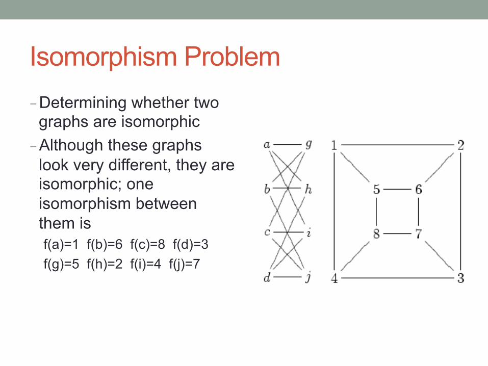
Isomorphism Problem - Determining whether two
graphs are isomorphic - Although these graphs
look very different, they are isomorphic; one isomorphism between them is f(a)=1 f(b)=6 f(c)=8 f(d)=3 f(g)=5 f(h)=2 f(i)=4 f(j)=7
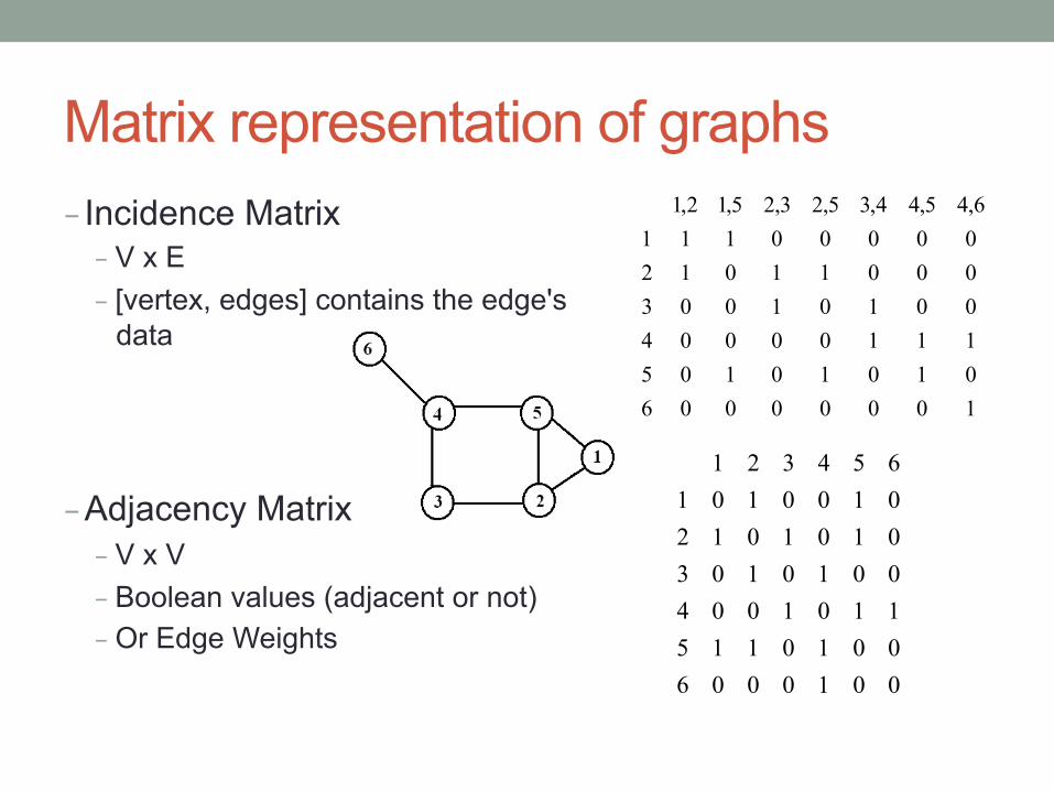
Matrix representation of graphs - Incidence Matrix - V x E - [vertex, edges] contains the edge's
data
- Adjacency Matrix - V x V - Boolean values (adjacent or not) - Or Edge Weights
1000000601010105111000040010100300011012000001116,45,44,35,23,25,12,1
001000600101151101004001010301010120100101654321
List representation of graphs - Edge List - pairs (ordered if directed) of vertices - Optionally weight and other data
- Adjacency List (node list)
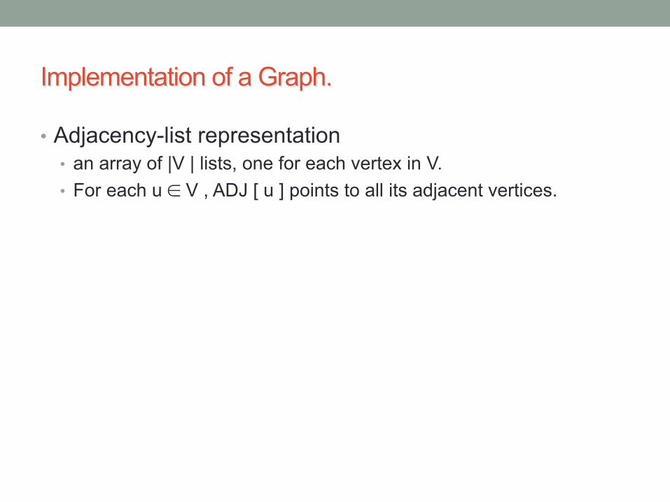
Implementation of a Graph.
• Adjacency-list representation • an array of |V | lists, one for each vertex in V. • For each u ∈ V , ADJ [ u ] points to all its adjacent vertices.
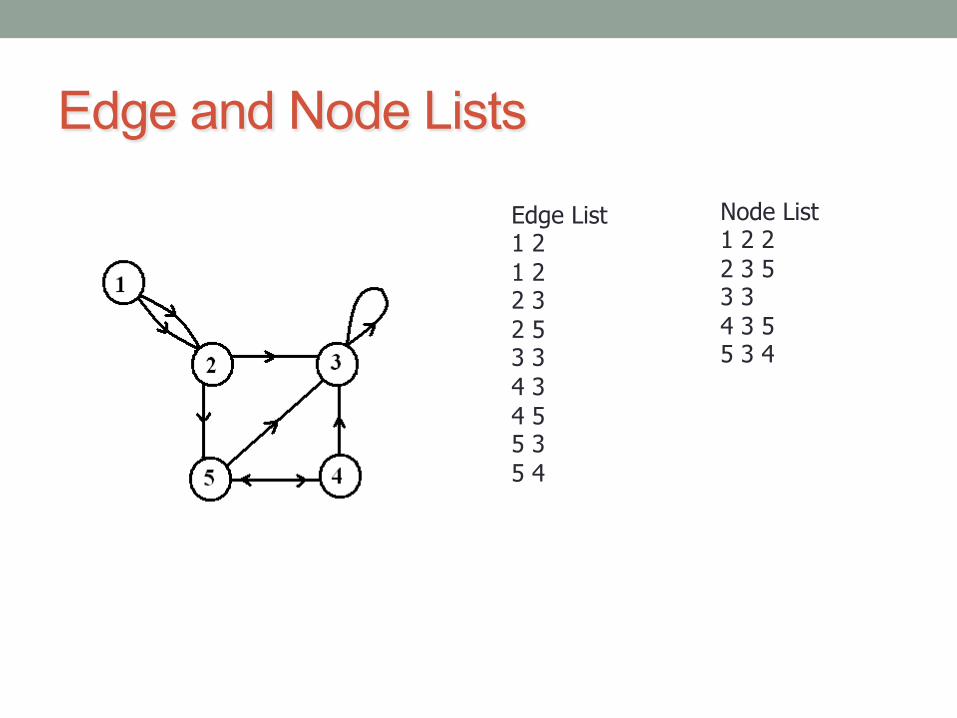
Edge and Node Lists
Edge List 1 2 1 2 2 3 2 5 3 3 4 3 4 5 5 3 5 4
Node List 1 2 2 2 3 5 3 3 4 3 5 5 3 4
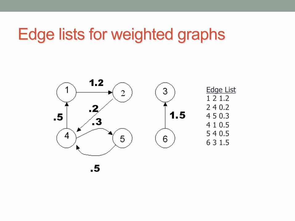
Edge lists for weighted graphs
Edge List 1 2 1.2 2 4 0.2 4 5 0.3 4 1 0.5 5 4 0.5 6 3 1.5
Topological Distance - A shortest path is the minimum path connecting two
nodes.
- The number of edges in the shortest path connecting p and q is the topological distance between these two nodes, dp,q
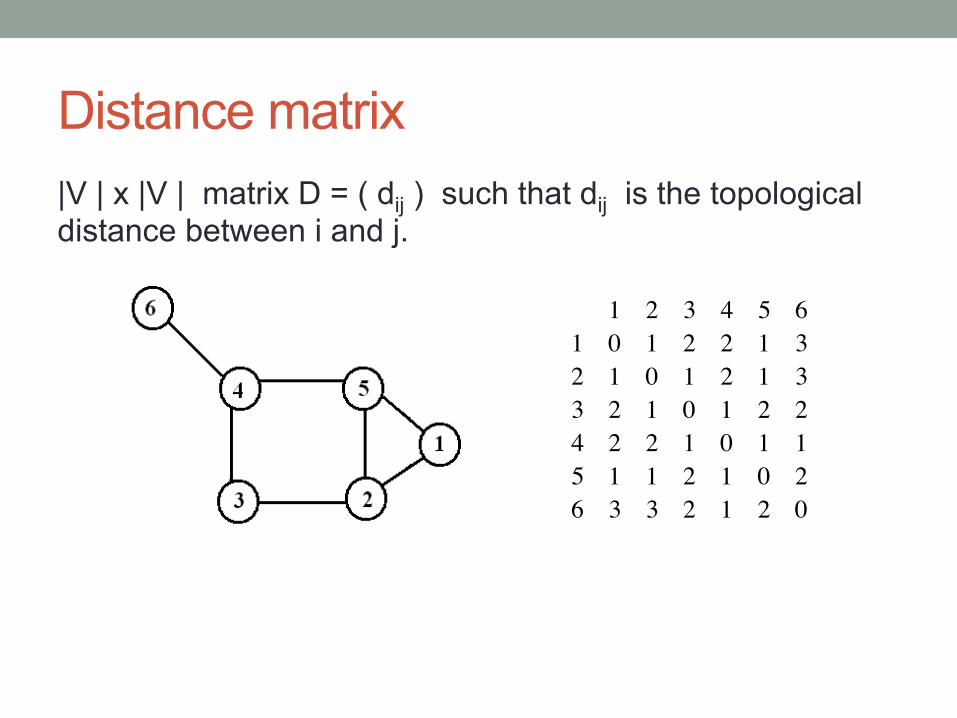
Distance matrix |V | x |V | matrix D = ( dij ) such that dij is the topological distance between i and j.
1 2 3 4 5 61 0 1 2 2 1 32 1 0 1 2 1 33 2 1 0 1 2 24 2 2 1 0 1 15 1 1 2 1 0 26 3 3 2 1 2 0
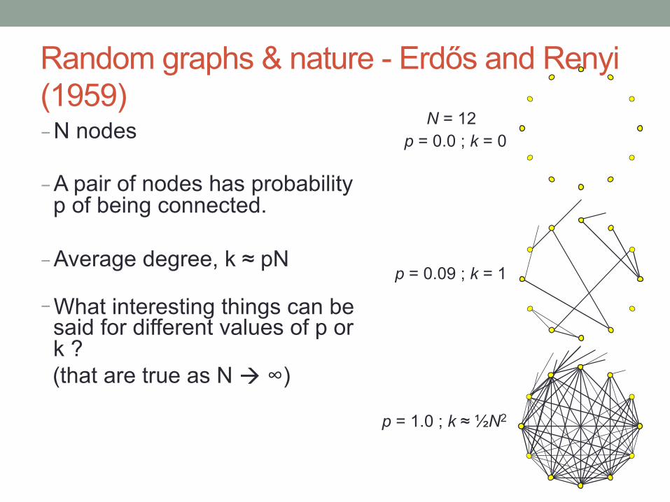
Random graphs & nature - Erdős and Renyi (1959) - N nodes
- A pair of nodes has probability p of being connected.
- Average degree, k ≈ pN
- What interesting things can be said for different values of p or k ?
(that are true as N à ∞)
p = 0.0 ; k = 0 N = 12
p = 0.09 ; k = 1
p = 1.0 ; k ≈ ½N2
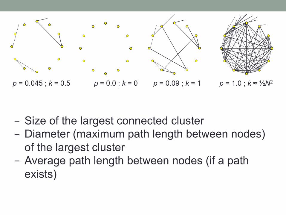
p = 0.0 ; k = 0 p = 0.09 ; k = 1 p = 1.0 ; k ≈ ½N2 p = 0.045 ; k = 0.5
- Size of the largest connected cluster - Diameter (maximum path length between nodes)
of the largest cluster - Average path length between nodes (if a path
exists)
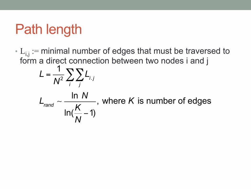
Path length • Li,j := minimal number of edges that must be traversed to
form a direct connection between two nodes i and j
L = 1N2
Li . jj∑
i∑
Lrand ln N
ln(KN−1)
, where K is number of edges
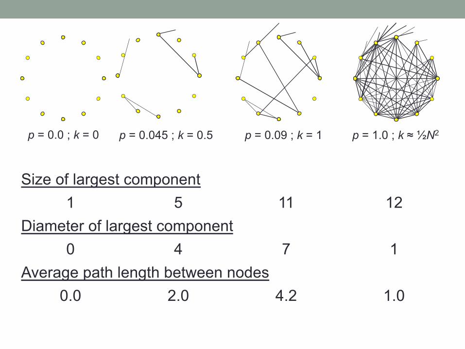
p = 0.0 ; k = 0 p = 0.09 ; k = 1 p = 1.0 ; k ≈ ½N2 p = 0.045 ; k = 0.5
Size of largest component 1 5 11 12
Diameter of largest component 0 4 7 1
Average path length between nodes 0.0 2.0 4.2 1.0
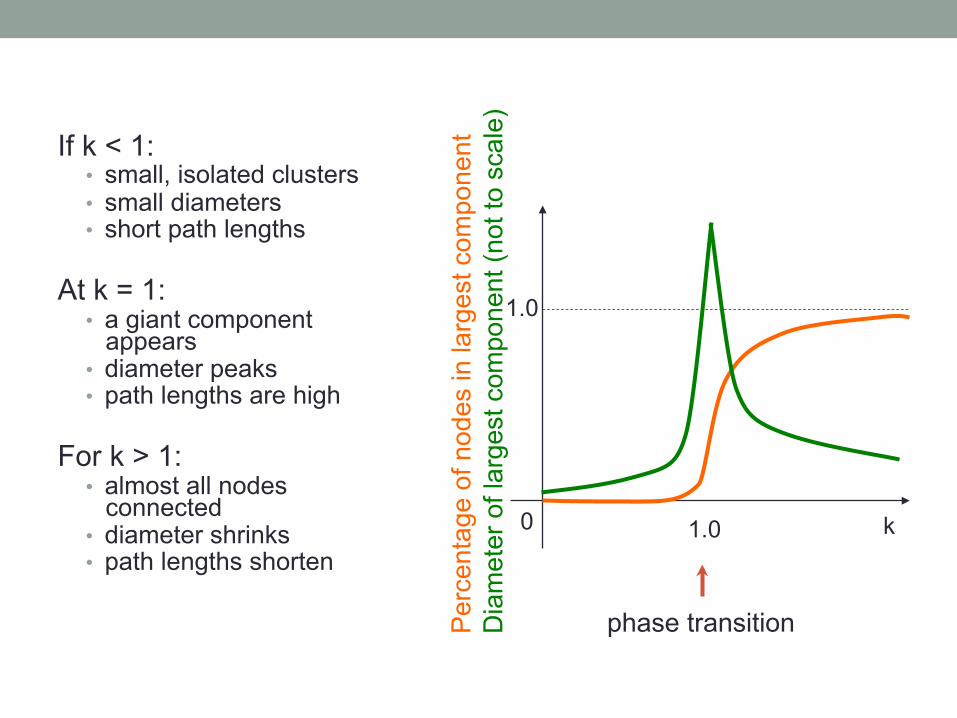
If k < 1: • small, isolated clusters • small diameters • short path lengths
At k = 1:
• a giant component appears
• diameter peaks • path lengths are high
For k > 1:
• almost all nodes connected
• diameter shrinks • path lengths shorten
Per
cent
age
of n
odes
in la
rges
t com
pone
nt
Dia
met
er o
f lar
gest
com
pone
nt (n
ot to
sca
le)
1.0
0 k 1.0
phase transition
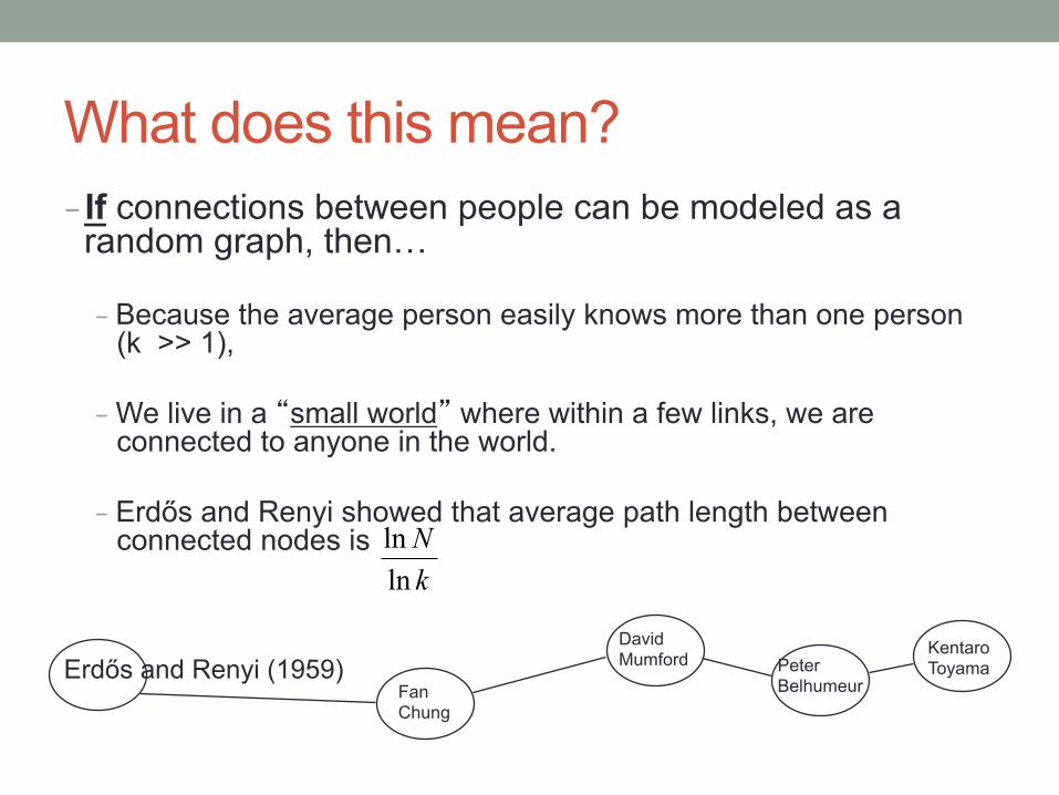
What does this mean? - If connections between people can be modeled as a
random graph, then…
- Because the average person easily knows more than one person (k >> 1),
- We live in a “small world” where within a few links, we are connected to anyone in the world.
- Erdős and Renyi showed that average path length between connected nodes is
Erdős and Renyi (1959) David Mumford Peter
Belhumeur
Kentaro Toyama
Fan Chung
kN
lnln
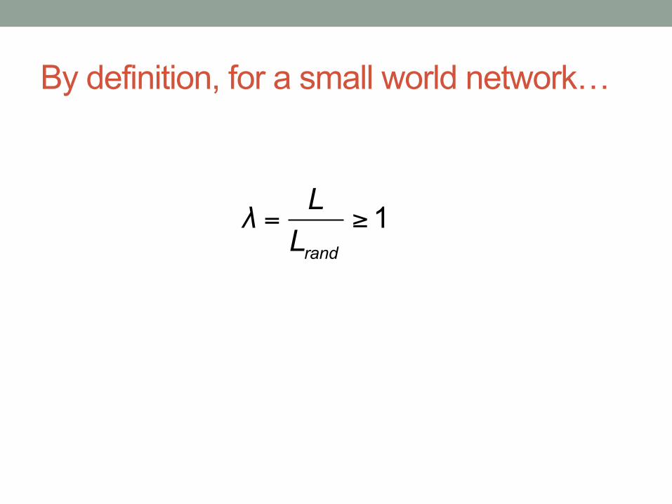
By definition, for a small world network…
1rand
LλL
= ≥
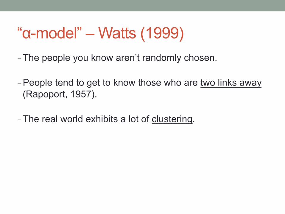
“α-model” – Watts (1999) - The people you know aren’t randomly chosen.
- People tend to get to know those who are two links away (Rapoport, 1957).
- The real world exhibits a lot of clustering.
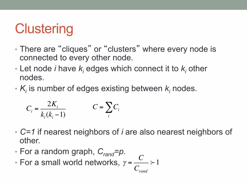
Clustering • There are “cliques” or “clusters” where every node is
connected to every other node. • Let node i have ki edges which connect it to ki other
nodes. • Ki is number of edges existing between ki nodes.
• C=1 if nearest neighbors of i are also nearest neighbors of
other. • For a random graph, Crand=p. • For a small world networks,
Ci =2Ki
ki (ki −1)C = Ci
i∑
γ =CCrand
1
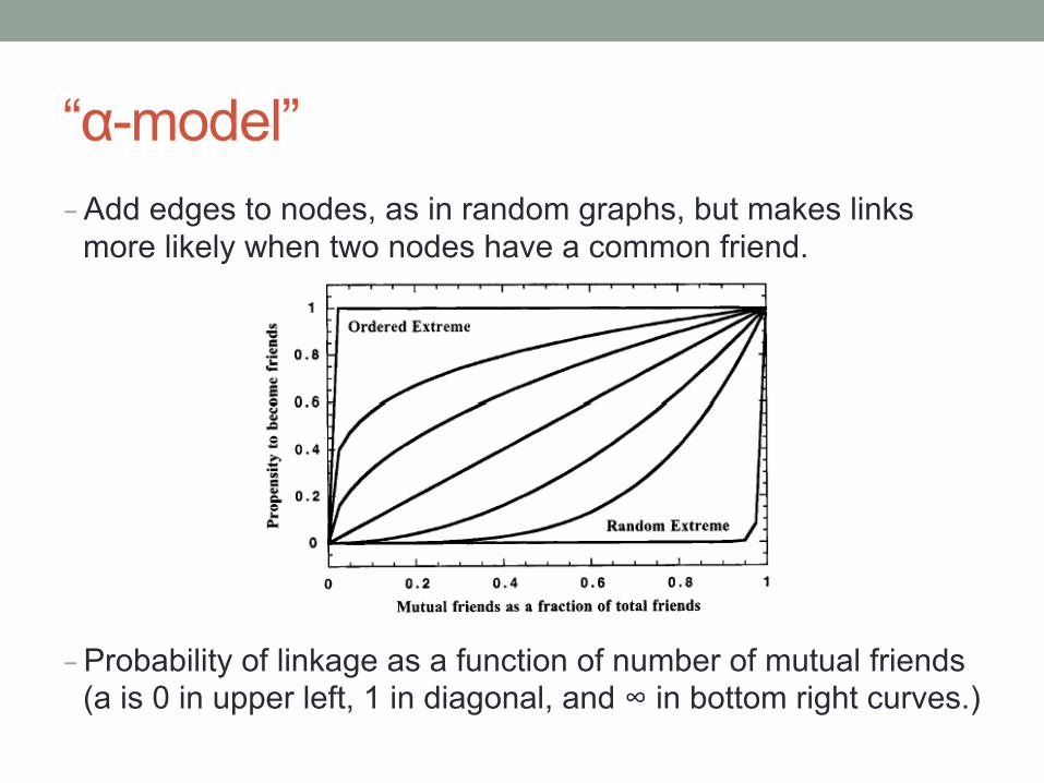
“α-model” - Add edges to nodes, as in random graphs, but makes links
more likely when two nodes have a common friend.
- Probability of linkage as a function of number of mutual friends (a is 0 in upper left, 1 in diagonal, and ∞ in bottom right curves.)
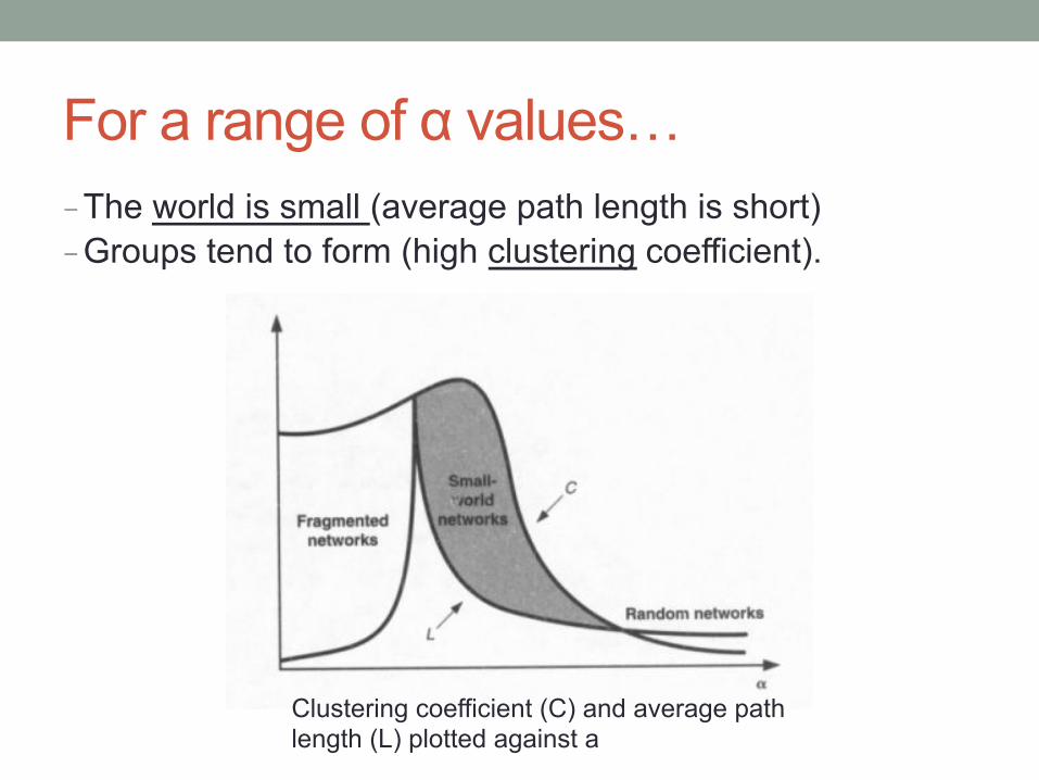
For a range of α values… - The world is small (average path length is short) - Groups tend to form (high clustering coefficient).
α Clustering coefficient (C) and average path length (L) plotted against a
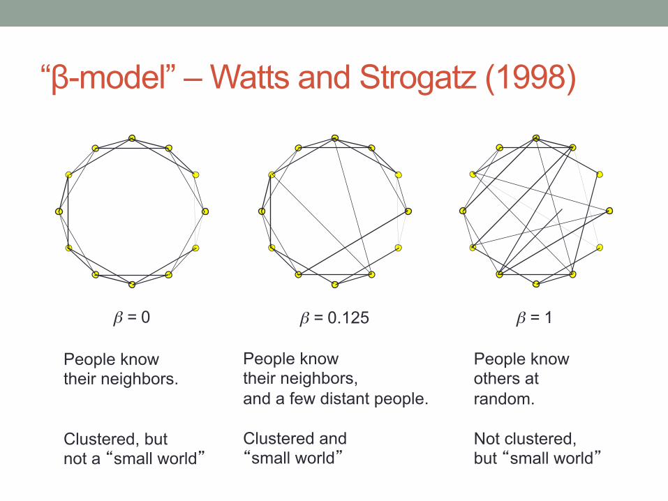
“β-model” – Watts and Strogatz (1998)
β = 0 β = 0.125 β = 1
People know others at random. Not clustered, but “small world”
People know their neighbors, and a few distant people. Clustered and “small world”
People know their neighbors. Clustered, but not a “small world”
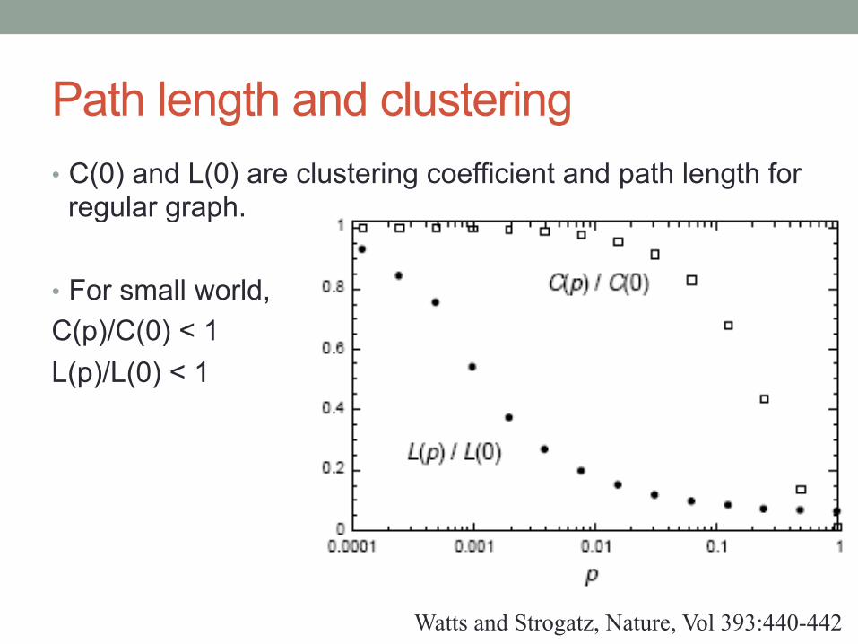
Path length and clustering • C(0) and L(0) are clustering coefficient and path length for
regular graph.
• For small world, C(p)/C(0) < 1 L(p)/L(0) < 1
Watts and Strogatz, Nature, Vol 393:440-442
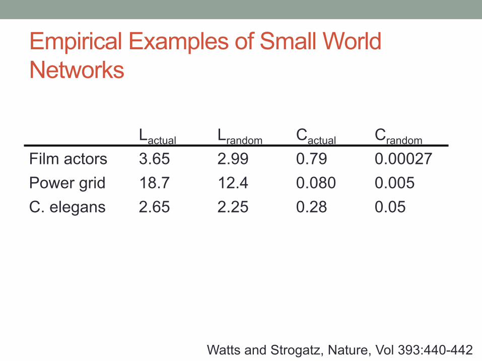
Empirical Examples of Small World Networks
Watts and Strogatz, Nature, Vol 393:440-442
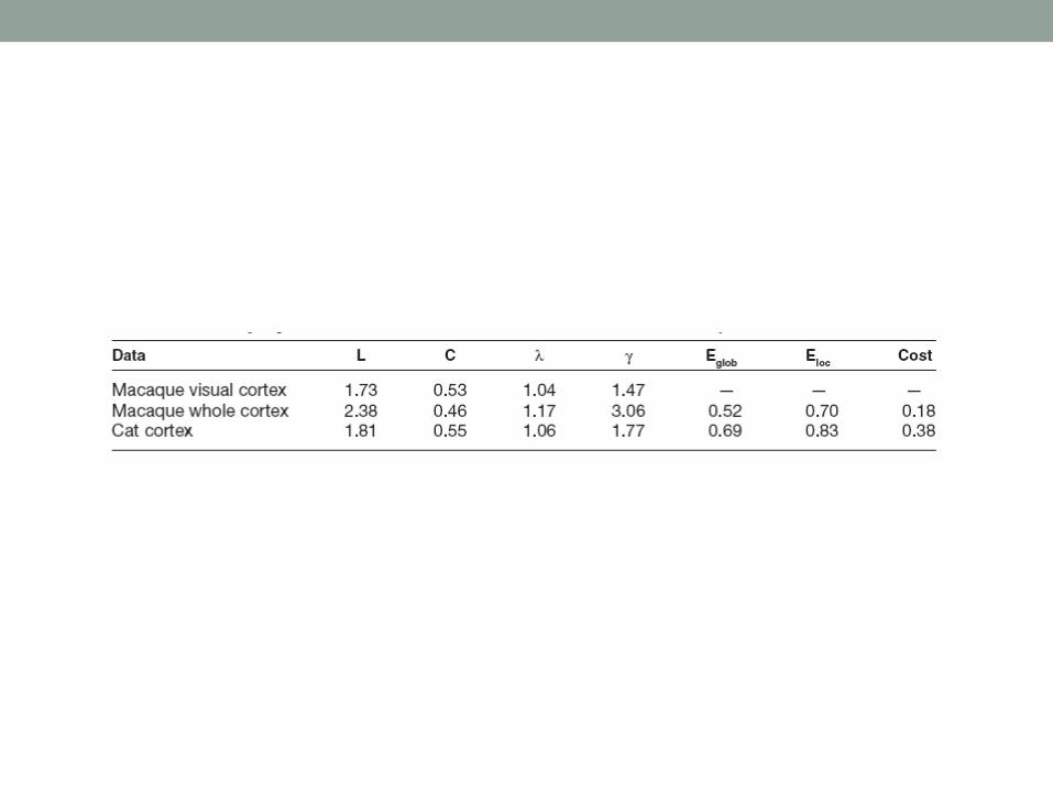
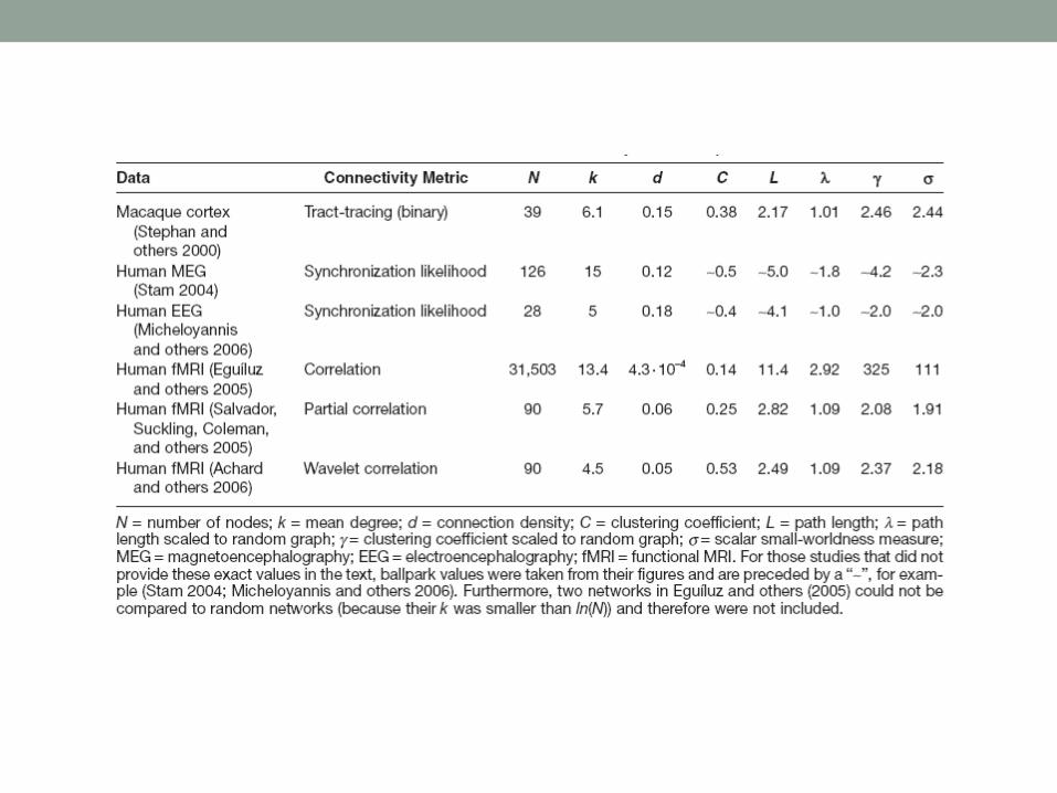
Lactual Lrandom Cactual Crandom Film actors 3.65 2.99 0.79 0.00027 Power grid 18.7 12.4 0.080 0.005 C. elegans 2.65 2.25 0.28 0.05
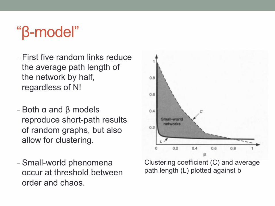
“β-model” - First five random links reduce
the average path length of the network by half, regardless of N!
- Both α and β models reproduce short-path results of random graphs, but also allow for clustering.
- Small-world phenomena occur at threshold between order and chaos.
Clustering coefficient (C) and average path length (L) plotted against b
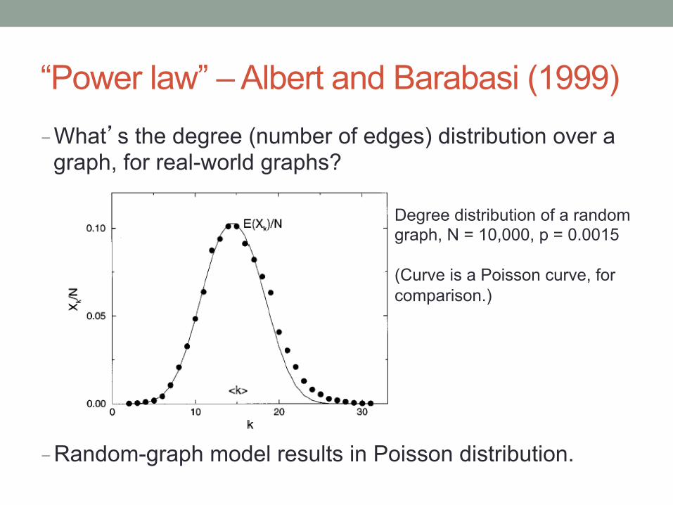
“Power law” – Albert and Barabasi (1999) - What’s the degree (number of edges) distribution over a
graph, for real-world graphs?
- Random-graph model results in Poisson distribution.
Degree distribution of a random graph, N = 10,000, p = 0.0015 (Curve is a Poisson curve, for comparison.)
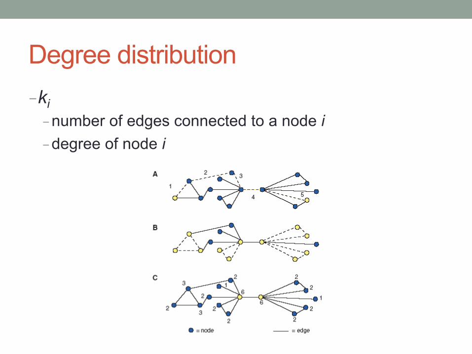
Degree distribution - ki - number of edges connected to a node i - degree of node i
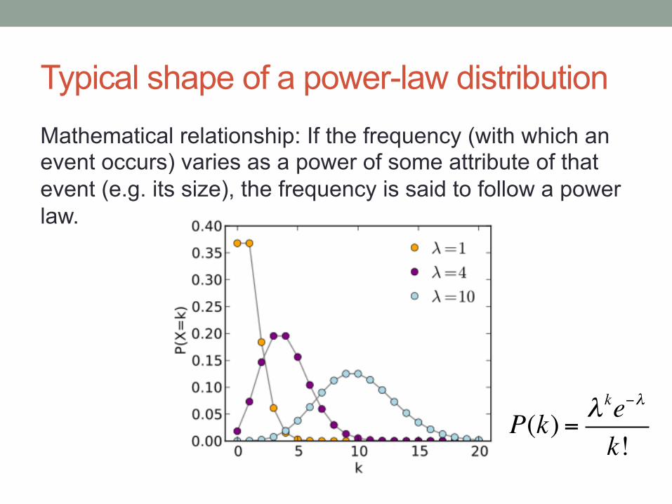
Typical shape of a power-law distribution Mathematical relationship: If the frequency (with which an event occurs) varies as a power of some attribute of that event (e.g. its size), the frequency is said to follow a power law.
P(k) = λke−λ
k!
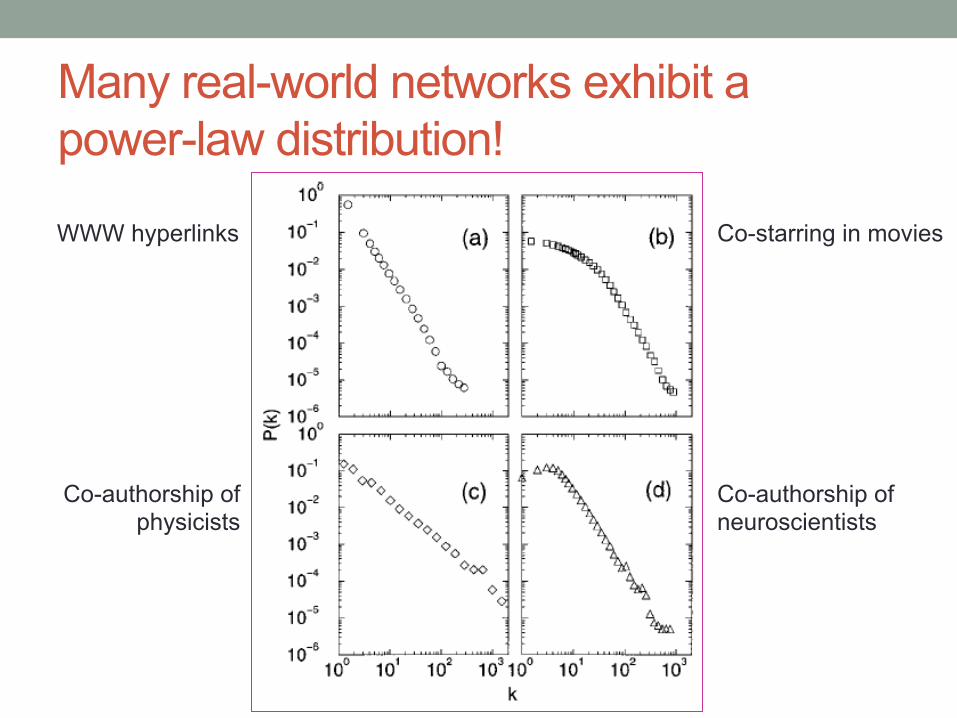
Many real-world networks exhibit a power-law distribution!
WWW hyperlinks
Co-authorship of physicists
Co-starring in movies
Co-authorship of neuroscientists
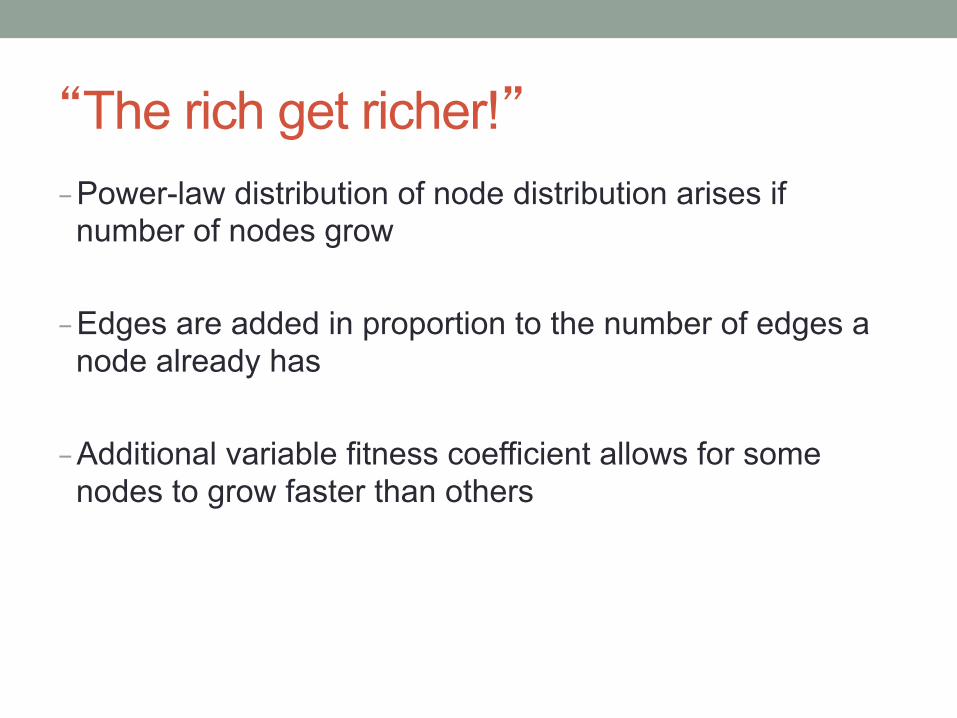
“The rich get richer!” - Power-law distribution of node distribution arises if
number of nodes grow
- Edges are added in proportion to the number of edges a node already has
- Additional variable fitness coefficient allows for some nodes to grow faster than others
Recap… - Are real networks fundamentally random?
- Intuitively, complex systems must display some organizing principles, which must be encoded in their topology
- arrangement in which the nodes of the network are connected to each other
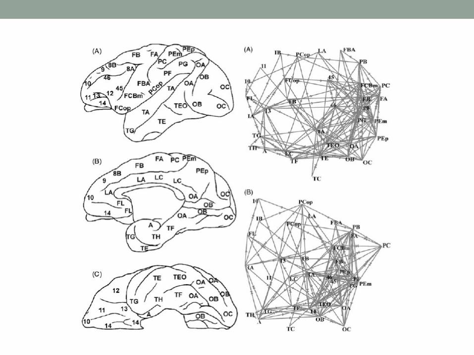
Why should we think about the brain as a small world network? - Brain is a complex network on multiple spatial and time scales - Connectivity of neurons
- Brain supports segregated and distributed information processing - Somatosensory and visual systems segregated - Distributed processing, executive functions
- Brain likely evolved to maximize efficiency and minimize the costs of information processing - Small world topology is associated with high global and local efficiency
of parallel information processing, sparse connectivity between nodes, and low wiring costs
- Adaptive reconfiguration
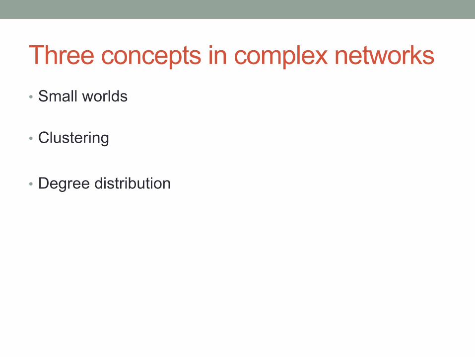
Three concepts in complex networks • Small worlds
• Clustering
• Degree distribution
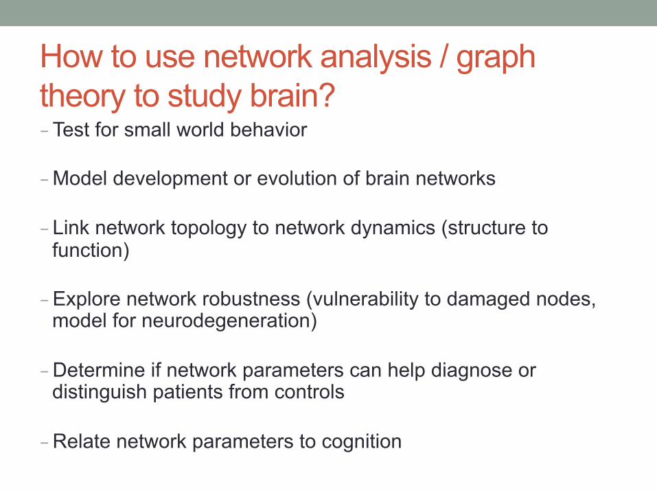
How to use network analysis / graph theory to study brain? - Test for small world behavior
- Model development or evolution of brain networks
- Link network topology to network dynamics (structure to function)
- Explore network robustness (vulnerability to damaged nodes, model for neurodegeneration)
- Determine if network parameters can help diagnose or distinguish patients from controls
- Relate network parameters to cognition
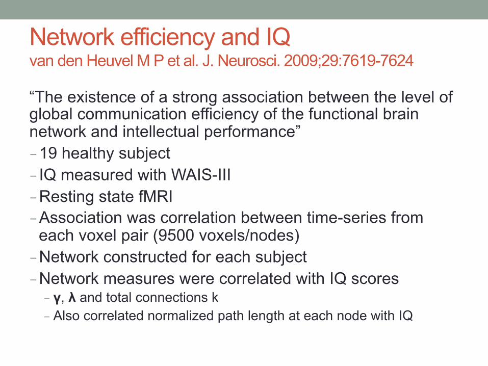
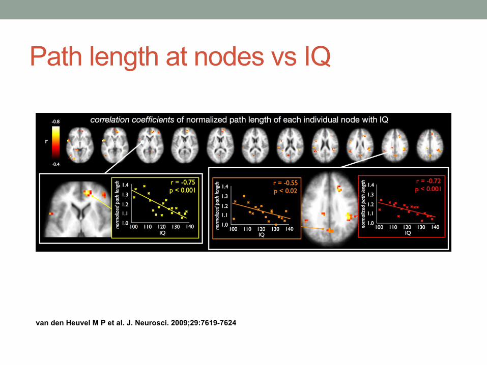
Network efficiency and IQ van den Heuvel M P et al. J. Neurosci. 2009;29:7619-7624 “The existence of a strong association between the level of global communication efficiency of the functional brain network and intellectual performance” - 19 healthy subject - IQ measured with WAIS-III - Resting state fMRI - Association was correlation between time-series from
each voxel pair (9500 voxels/nodes) - Network constructed for each subject - Network measures were correlated with IQ scores - γ, λ and total connections k - Also correlated normalized path length at each node with IQ
van den Heuvel M P et al. J. Neurosci. 2009;29:7619-7624
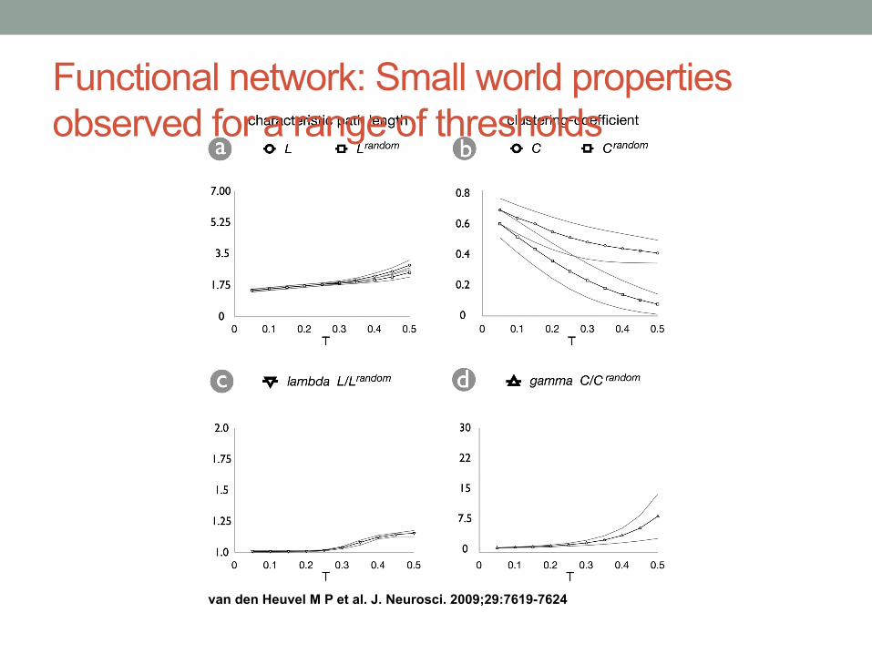
Functional network: Small world properties observed for a range of thresholds
van den Heuvel M P et al. J. Neurosci. 2009;29:7619-7624
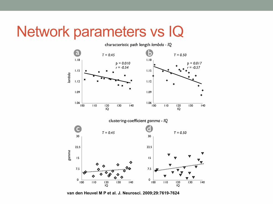
Network parameters vs IQ
van den Heuvel M P et al. J. Neurosci. 2009;29:7619-7624
Path length at nodes vs IQ
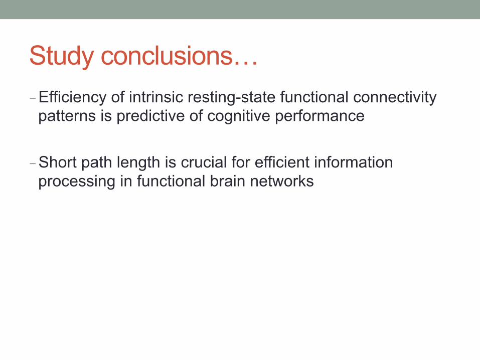
Study conclusions… - Efficiency of intrinsic resting-state functional connectivity
patterns is predictive of cognitive performance
- Short path length is crucial for efficient information processing in functional brain networks
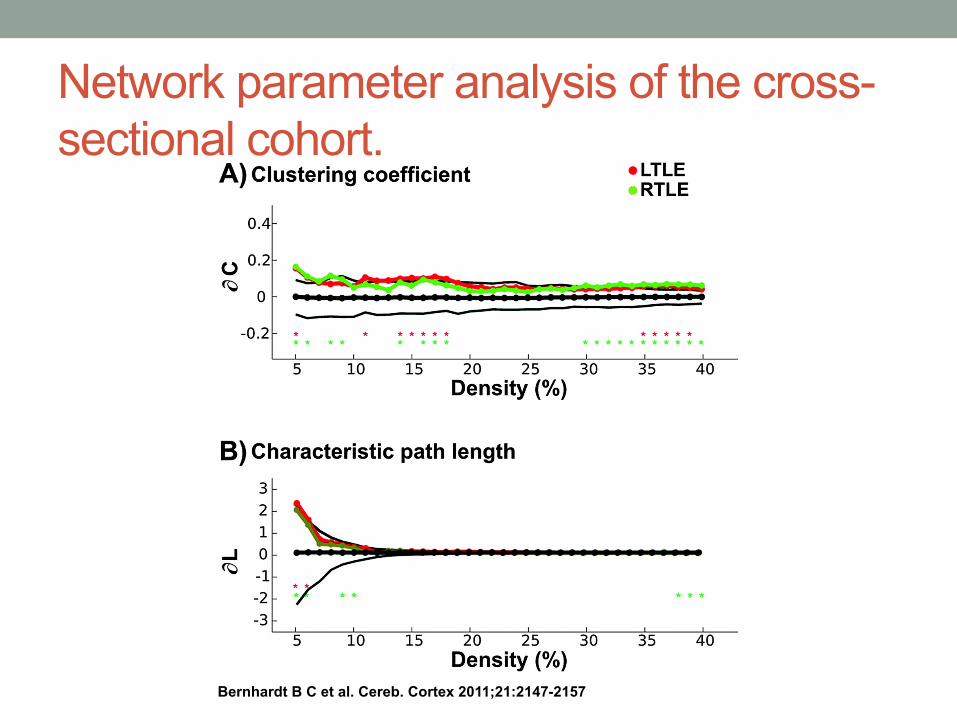
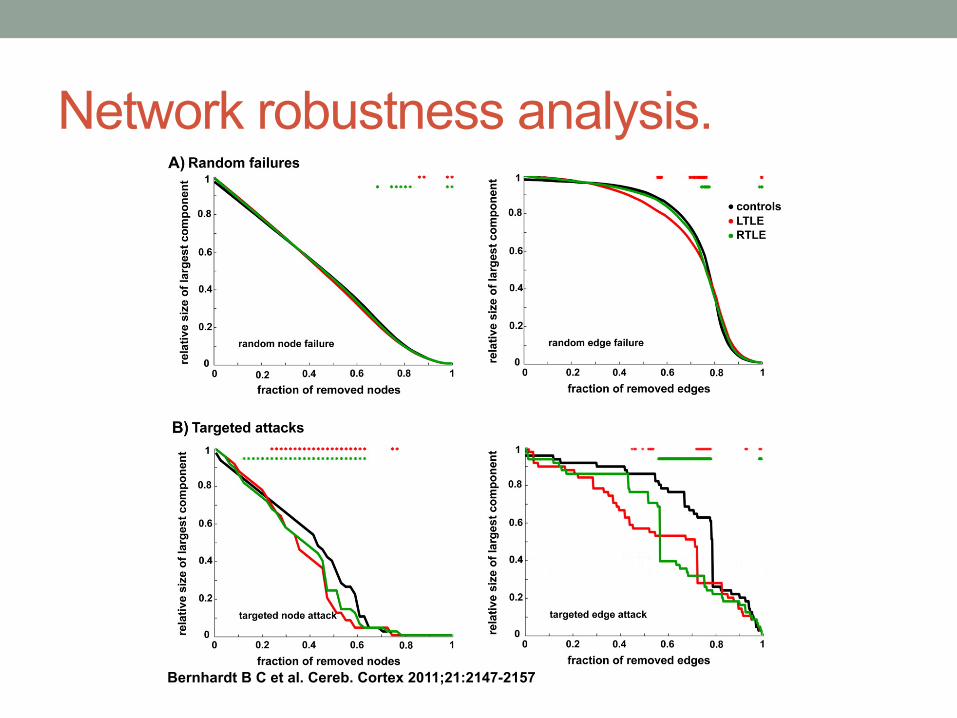
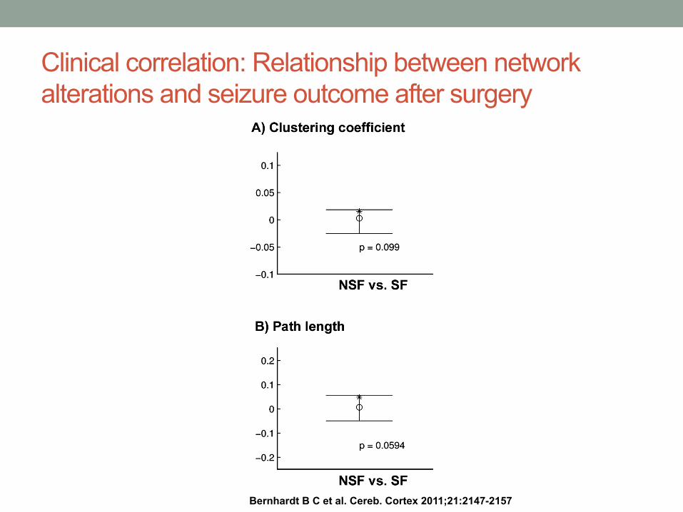
Cortical Thickness Networks in Temporal Lobe Epilepsy Bernhardt B C et al. Cereb. Cortex 2011;21:2147-2157 - 122 patients with drug-resistant TLE; 63 LTLE, 59 RTLE - 47 age- and sex-matched healthy controls - T1-weighted imaging at 1.5T - Estimated cortical thickness in 52 ROIs - Thicknesses corrected for age, gender, overall mean thickness
- Computed rij Pearson product moment cross-correlation across subjects in regions i and j - Explored network parameters at a range of connection
densities - Different networks for controls, LTLE, RTLE - Ensures that networks in all groups have the same number of edges or
wiring cost - Between group differences reflect topological organization differences;
not differences in correlations
Bernhardt B C et al. Cereb. Cortex 2011;21:2147-2157
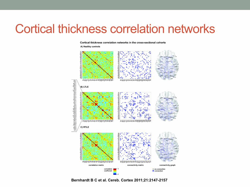
Cortical thickness correlation networks
Bernhardt B C et al. Cereb. Cortex 2011;21:2147-2157
Network parameter analysis of the cross-sectional cohort.
Bernhardt B C et al. Cereb. Cortex 2011;21:2147-2157
Network robustness analysis.
Bernhardt B C et al. Cereb. Cortex 2011;21:2147-2157
Clinical correlation: Relationship between network alterations and seizure outcome after surgery
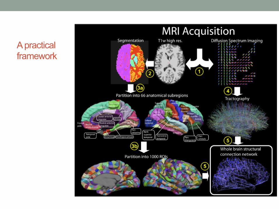
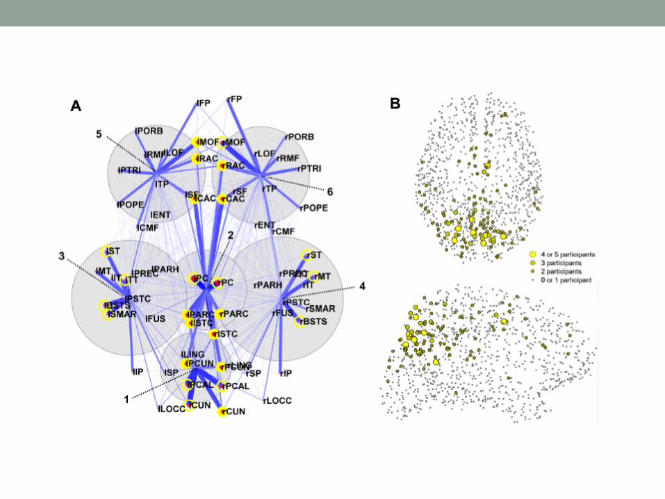
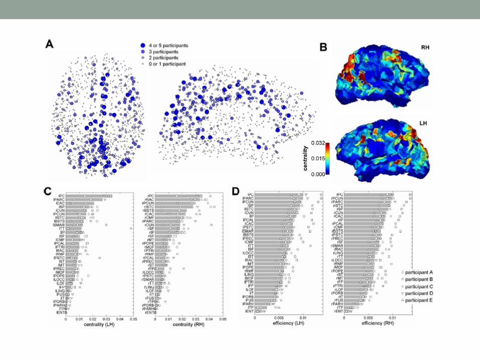
A practical framework
References - Duncan Watts, Six Degrees (2003). - Albert and Barabasi, “Statistical mechanics of complex networks.” Review of
Modern Physics. 74:48-94. (2002) - Kolaczyk, Statistical Analysis of Network Data: Methods and Models, Springer
2009. - Guye et al., Imaging of structural and functional connectivity: towards a unified
definiton of human brain organization? Current Opinion in Neurology 2008, 21:393-400.
- Bassett et al., Hierarchical organization of human cortical networks in health and schizophrenia schizophrenia. The Journal of Neuroscience, 2009, 28(37):9239-9248.
- Van den Heuvel et al., Efficiency of functional brain networks and intellectual performance. The Journal of Neuroscience, 2009, 29(23):7619-7624.
- Bassett and Bullmore, Small-World Brain Networks. The Neuroscientist, 2006, 12(6):512-523.
- Bullmore and Sporns, Complex brain networks: graph theorectical analysis of structural and functional systems. Nature Reviews: Neuroscience, 2009, 10:186-198.
- Telesford et al., Reproducilbility of graph metrics in fMRI networks. Frontiers in Neuroscience, 2010, 4:article 117.
Network / graph analysis software - Brain connectivity toolbox http://www.brain-connectivity-toolbox.net
- Matlab BGL - http://www.stanford.edu/~dgleich/programs/matlab_bgl