Net primary production of terrestrial ecosystems in Chinaand its equilibrium responses to changes in climate and

atmospheric CO2 concentration

X. Xiao1,2, J.M. Melillo1, D.W. Kicklighter1, Y. Pan1, A.D. McGuire3 and J. Helfrich1

1The Ecosystems Center, Marine Biological Laboratory, Woods Hole, MA 025432The Joint Program on the Science and Policy of Global Change,Massachusetts Institute of Technology, Cambridge, MA 02139

3Institute of Arctic Biology, University of Alaska, Fairbanks, AK 99775

Abstract

We used the Terrestrial Ecosystem Model (TEM, version 4.0) to estimate net primaryproduction (NPP) in China for contemporary climate and NPP responses to elevated CO2 andclimate changes projected by three atmospheric general circulation models (GCMs): GoddardInstitute for Space Studies (GISS), Geophysical Fluid Dynamic Laboratory (GFDL) and OregonState University (OSU). For contemporary climate at 312.5 ppmv CO2, TEM estimates that Chinahas an annual NPP of 3,653 TgC yr-1 (1012 gC yr-1). Temperate broadleaf evergreen forest is themost productive biome and accounts for the largest portion of annual NPP in China. The spatialpattern of NPP is closely correlated to the spatial distributions of precipitation and temperature.

Annual NPP of China is sensitive to changes in CO2 and climate. At the continental scale,annual NPP of China increases by 6.0% (219 TgC yr-1) for elevated CO2 only (519 ppmv CO2).For climate change with no change in CO2, the response of annual NPP ranges from a decrease of1.5% (54.8 TgC yr-1) for the GISS climate to an increase of 8.4% (306.9 TgC yr-1) for theGFDL-q climate. For climate change at 519 ppmv CO2, annual NPP of China increasessubstantially, ranging from 18.7% (683 TgC yr-1) for the GISS climate to 23.3% (851 TgC yr-1)for the GFDL-q climate. Spatially, the responses of annual NPP to changes in climate and CO2

vary considerably within a GCM climate. Differences among the three GCM climates used in thestudy cause large differences in the geographical distribution of NPP responses to projected climatechanges. The interaction between elevated CO2 and climate change plays an important role in theoverall response of NPP to climate change at 519 ppmv CO2.

Submitted to: Acta Phytoecologica Sinica (published in China)Author responsible for correspondence: Dr. Xiangming Xiao, The Ecosystems Center, Marine Biological Laboratory,

Woods Hole, MA 02543, Tel: (508)289-7498, Fax: (508)457-1548, Email: xiao@lupine.mbl.eduKey words: spatial patterns, climate models, ecosystem models, impact assessment

2

1. Introduction

Atmospheric concentrations of CO2 and other long-lived greenhouse gases (e.g., N2O) willcontinue to increase in the next century as the result of increasing anthropogenic emissions of thesetrace gases. Increasing greenhouse gases will further increase the radiative forcing of climate. Fordoubled CO2, a number of atmospheric general circulation models (GCMs) estimate that globallyaveraged surface air temperature will increase in the range of 1.5 ˚C to 4.5 ˚C (Mitchell, et al.,1990). Globally, there are also large geographical variations in the changes of precipitation andclouds projected by GCMs. The increasing atmospheric CO2 concentration and resultant climatechange are likely to have significant impacts on net primary production of terrestrial ecosystems(Melillo, et al., 1990). Net primary production of terrestrial ecosystems is important in estimatingland carrying capacity, which is critically relevant to the social and economic development of acountry like China. China has a very large human population (about 1⁄5 of the world population)and limited natural resources, especially fertile lands. The total land area in China is only about1⁄15 of the world land area and about 65% of this area is hills, mountains and plateau (Xiong andLi, 1988).

In China, the magnitude and spatial patterns of temperature and precipitation will changesignificantly according to simulations of a GCM for a doubling of atmospheric CO2 concentration(Zhang and Wang, 1993; Wang and Zhang, 1993). Few studies have examined impacts of climatechange on net primary production (NPP) of natural ecosystems in China (Zhang, 1993; Xiao, etal., 1995). Zhang (1993) applied a regression model (Chikugo model, Uchijima and Seino, 1985),which uses annual values of climate variables (e.g., temperature, precipitation, relative humidity)to estimate NPP of various ecosystems in China for contemporary climate. Zhang (1993) alsocalculated the responses of NPP to: (1) +2 ˚C and 20% increase of annual precipitation, and(2) +4 ˚C and 20% increase of annual precipitation in China. Net primary production increases forall the vegetation types under these climate change conditions (Zhang, 1993). However, theChikugo model is basically a regression model based on correlation between NPP and climate, andthe model has not considered the possible limitations of nutrient availability (e.g., nitrogen) onNPP. Generally, the potential of application of regression models for future projection is limitedbecause the regressions may not be appropriate for climatic conditions that are novel to terrestrialecosystems (Melillo, et al., 1993).

Recently, a number of processed-based ecosystem models, which are integrated withgeographically referenced spatial data, have been applied to estimate responses of NPP and carbonstorage to changes in climate and atmospheric CO2 concentration at the global scale (Melillo, et al.,1993; McGuire, et al., 1995, 1996; Xiao, et al., 1996a) and the continental scale, e.g., SouthAmerica (Raich, et al., 1991), North America (McGuire, et al., 1992, 1993) and conterminousUnited States (VEMAP Members, 1995). Estimates of NPP responses vary among the GCMsused in the studies across the scales of grid cell, biome, continent and the globe (Melillo, et al.,1993; VEMAP, 1995; Xiao, et al., 1996a). The process-based ecosystem models integrate keyecosystem processes such as plant photosynthesis, plant respiration, decomposition of soil organic

3

matter and nutrient cycling, which interactively affect NPP. These ecological processes arecontrolled by a number of abiotic factors, e.g., water, light, temperature, soil texture and nutrients.The simultaneous interactions among the dynamics of carbon, nitrogen and water are complex andspatially variable.

In this study, we used a process-based global terrestrial biogeochemistry model, theTerrestrial Ecosystem Model (Raich, et al., 1991; McGuire, et al., 1995, 1996). First, we appliedTEM to estimate the magnitude and spatial distribution of annual NPP of terrestrial ecosystems inChina for contemporary climate. Second, we applied TEM to quantify the equilibrium responses ofannual NPP in China to changes in atmospheric CO2 concentration and climate projected by threeGCMs. We examined the TEM simulation results across the spatial scales of grid cell, biome andcontinent. The analysis will help us to understand how the abiotic factors (e.g., climate, soiltexture) control the magnitude and spatial distribution of NPP in China.

2. Model and Data

2.1 The Terrestrial Ecosystem Model (TEM)

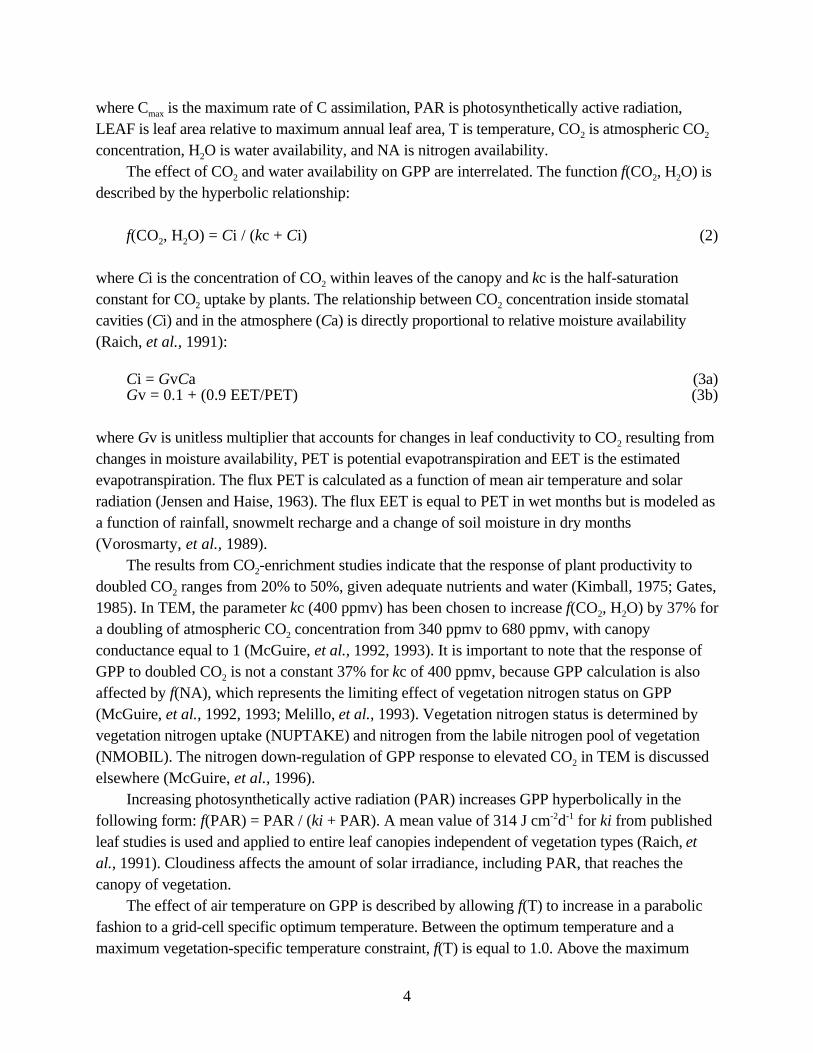
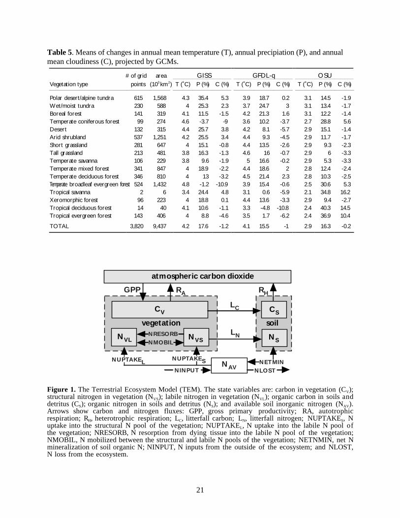
The TEM (Figure 1) is a process-based ecosystem model that simulates important carbon andnitrogen fluxes and pools for various terrestrial biomes (Raich, et al., 1991; McGuire, et al., 1992,1993, 1995). The TEM has been used to examine patterns of net primary production (NPP) inSouth America (Raich, et al., 1991) and North America (McGuire, et al., 1992) for contemporaryclimate. The model has also been used to estimate the responses of NPP of the terrestrial biosphereto climate change projected by four GCMs (Melillo, et al., 1993). In this study, we use version 4.0of TEM, which was modified from TEM version 3 to improve patterns of soil organic carbonstorage along gradients of temperature, moisture and soil texture (McGuire, et al., 1995, 1996).Version 4.0 of TEM has also been used to estimate the responses of NPP and carbon storage ofterrestrial ecosystems to climate change in the conterminous United State (VEMAP Members,1995; Pan, et al., 1996a) and at the global scale (McGuire, et al., 1996; Xiao, et al., 1996a,1996b). Detailed descriptions of TEM are documented in Raich, et al. (1991) and McGuire, et al.(1992). The recent TEM modifications are presented elsewhere (McGuire, et al., 1995, 1996). Tohelp understand how climate change and elevated CO2 influence NPP in TEM, we review the keyprocesses related to NPP.

Net primary production (NPP) is calculated as the difference between gross primaryproduction (GPP) and plant respiration (RA). The flux GPP is calculated at each monthly time stepas follows:

GPP = Cmax f(PAR) f(LEAF) f(T) f(CO2, H2O) f(NA) (1)

4

where Cmax is the maximum rate of C assimilation, PAR is photosynthetically active radiation,LEAF is leaf area relative to maximum annual leaf area, T is temperature, CO2 is atmospheric CO2

concentration, H2O is water availability, and NA is nitrogen availability.The effect of CO2 and water availability on GPP are interrelated. The function f(CO2, H2O) is

described by the hyperbolic relationship:

f(CO2, H2O) = Ci / (kc + Ci) (2)

where Ci is the concentration of CO2 within leaves of the canopy and kc is the half-saturationconstant for CO2 uptake by plants. The relationship between CO2 concentration inside stomatalcavities (Ci) and in the atmosphere (Ca) is directly proportional to relative moisture availability(Raich, et al., 1991):

Ci = GvCa (3a)Gv = 0.1 + (0.9 EET/PET) (3b)

where Gv is unitless multiplier that accounts for changes in leaf conductivity to CO2 resulting fromchanges in moisture availability, PET is potential evapotranspiration and EET is the estimatedevapotranspiration. The flux PET is calculated as a function of mean air temperature and solarradiation (Jensen and Haise, 1963). The flux EET is equal to PET in wet months but is modeled asa function of rainfall, snowmelt recharge and a change of soil moisture in dry months(Vorosmarty, et al., 1989).

The results from CO2-enrichment studies indicate that the response of plant productivity todoubled CO2 ranges from 20% to 50%, given adequate nutrients and water (Kimball, 1975; Gates,1985). In TEM, the parameter kc (400 ppmv) has been chosen to increase f(CO2, H2O) by 37% fora doubling of atmospheric CO2 concentration from 340 ppmv to 680 ppmv, with canopyconductance equal to 1 (McGuire, et al., 1992, 1993). It is important to note that the response ofGPP to doubled CO2 is not a constant 37% for kc of 400 ppmv, because GPP calculation is alsoaffected by f(NA), which represents the limiting effect of vegetation nitrogen status on GPP(McGuire, et al., 1992, 1993; Melillo, et al., 1993). Vegetation nitrogen status is determined byvegetation nitrogen uptake (NUPTAKE) and nitrogen from the labile nitrogen pool of vegetation(NMOBIL). The nitrogen down-regulation of GPP response to elevated CO2 in TEM is discussedelsewhere (McGuire, et al., 1996).

Increasing photosynthetically active radiation (PAR) increases GPP hyperbolically in thefollowing form: f(PAR) = PAR / (ki + PAR). A mean value of 314 J cm-2d-1 for ki from publishedleaf studies is used and applied to entire leaf canopies independent of vegetation types (Raich, etal., 1991). Cloudiness affects the amount of solar irradiance, including PAR, that reaches thecanopy of vegetation.

The effect of air temperature on GPP is described by allowing f(T) to increase in a parabolicfashion to a grid-cell specific optimum temperature. Between the optimum temperature and amaximum vegetation-specific temperature constraint, f(T) is equal to 1.0. Above the maximum

5

temperature constraint, f(T) declines rapidly to 0.0 (McGuire, et al., 1996). Air temperature alsoaffects plant respiration (RA). The flux RA includes both maintenance respiration (RM) andconstruction respiration (RC). The flux RM increases logarithmically with temperature using a Q10

value that varies from 1.5 to 2.5 (McGuire, et al., 1992). The flux RC is determined to be 20% ofthe difference between GPP and RM (Raich, et al., 1991). Thus, changes in NPP are directlyrelated to changes in CO2, temperature, precipitation and cloudiness.

The simulation of TEM requires the use of soil- and vegetation-specific parameters appropriateto an ecosystem type. Although many of the vegetation-specific parameters in the model aredefined from published references, some are determined by calibrating TEM to the fluxes and poolsizes of an intensively studied field site. Most of the data used to calibrate TEM for the 18vegetation types of our global vegetation classification are documented elsewhere (Raich, et al.,1991; McGuire, et al., 1992, 1996).

2.2 Spatial data for extrapolation of TEM

The driving variables for the spatial extrapolation of TEM are vegetation types, elevation, soiltexture, monthly mean temperature, monthly precipitation, monthly mean cloudiness, and severalhydrological variables (potential evapotranspiration, estimated evapotranspiration and soilmoisture). Hydrological inputs for TEM are generated by a water balance model (Vorosmarty, etal., 1989) that uses the same climate, elevation, soils and vegetation data.

In this study, the spatial data used to drive TEM are derived from our global data sets(Melillo, et al., 1993; McGuire, et al., 1995, 1996; Xiao, et al., 1996a), which are organized in agrid at a 0.5˚ (latitude) × 0.5˚ (longitude) resolution. China has 3,852 grid cells, including six gridcells of inland water body and 26 grid cells of wetlands. The TEM does not estimate NPP andcarbon storage for grid cells defined as water or wetland ecosystems, so the extrapolation of TEMto China requires the application of TEM to 3820 grid cells.

We use potential vegetation in this study. Our global classification of potential vegetationincludes 18 upland biomes (Melillo, et al., 1993). In developing the global vegetation data, theVegetation Map of China (Hou, et al., 1982) was used in digitization and aggregation. There are16 upland biomes in China (Plate 1). Forests dominate in southern China and eastern coastal areas,while arid and semi-arid biomes prevail in northwestern China. The Qinhai-Tibet plateau isdominated by polar desert/alpine tundra.

For elevation, we use the NCAR/NAVY global 10-minute dataset (NCAR/NAVY, 1984)aggregated to a 0.5˚ resolution. Elevation increases from east to west in China (Plate 2a). TheQinhai-Tibet plateau has the highest elevation, mostly over 3000 m. The Mongolia Plateau andLoess plateau have elevation of 1000–1500 m.

For soil texture data, we use the FAO/CSRC/MBL data set (FAO/CSRC/MBL, undated),which is a digitization version of the FAO-UNESCO World Soil Map (FAO/Unesco, 1971) at 0.5˚grid resolution. There are seven texture classes in the FAO/CSRC/MBL data set that represents“average” soil profiles of the three FAO texture classes. Each FAO/CSRC/MBL soil texture class

6

defines a combination of sand, silt and clay proportions (Table 1). As shown in Plate 2b, soiltexture is generally more coarse in northern China than in southern China.

For contemporary climate, we use the long-term average climate data from the global climatedataset of Cramer and Leemans (Wolfgang Cramer, personal communication), which is an updateof an earlier version of global climate database (Leemans and Cramer,1990) that has monthlyprecipitation, temperature and sunshine duration. Monthly percent cloudiness is calculated as 100percent minus monthly percent sunshine duration. On the continental scale, annual meantemperature is about 5.8 ˚C, annual precipitation is about 661 mm and annual mean cloudiness is48%. Most precipitation occurs in the plant growing season (April to September). Geographically,annual mean temperature decreases gradually from south to north (Plate 2c). The Qinhai-TibetPlateau has very low annual mean temperature, because of high elevation. Annual precipitationdecreases from southeast to northwest, as affected by summer monsoon (Plate 2c). Vegetationdistribution in China (Plate 1) is closely correlated to spatial patterns of temperature andprecipitation (Plate 2). Characteristics of the climate variables for each of the 16 biomes are listed inTable 2. Tropical savanna has the highest annual mean temperature (24.2 ˚C) and annualprecipitation (1793 mm), while alpine tundra has the lowest annual mean temperature (−4.1 ˚C),and desert has the smallest amount of annual precipitation (74 mm).

2.3 Scenarios of climate change and elevated CO2

We first ran TEM for contemporary climate at 312.5 ppmv CO2 as the baseline forcomparison. We used 312.5 ppmv CO2 because it is the average value of atmospheric CO2

concentration for the 1 × CO2 simulations used by the GCMs described in Melillo, et al., (1993).To help separate the relative importance of elevated CO2 and climate changes, we then ran TEMunder (1) elevated CO2 only, (2) climate change only, and (3) climate change plus elevated CO2.For each of the four simulations, we ran TEM to steady state, therefore, its estimates of annualNPP apply only to mature, undisturbed vegetation and ecosystems. We have not considered theimpacts of changes in land use and land cover on NPP in this study.

For climate change predictions, we used climate outputs for “current” (1 × CO2) and“doubled” (2 × CO2) simulations from three GCMs, i.e., Geophysical Fluid Dynamic Laboratory(GFDL-q, Weatherald and Manabe, 1988), Goddard Institute for Space Studies (GISS, Hansen, etal., 1983, 1984) and Oregon State University (OSU, Schlesinger and Zhao, 1989). These GCMshave very coarse spatial resolutions, i.e., 10.0˚ (longitude) × 7.83˚ (latitude) for GISS, 7.5˚ ×4.44˚ for GFDL and 5.0˚ × 4.00˚ for OSU. In order to be consistent with the spatial resolution ofthe contemporary climate data, the outputs of the GCMs were interpolated to a 0.5˚ × 0.5˚ gridresolution by applying a spherical interpolation routine (Willmott, et al., 1985) to the data.

We calculated the differences in monthly mean temperature and the ratios in monthlyprecipitation and mean monthly cloudiness between the 2 × CO2 and 1 × CO2 simulations of theGCMs. The OSU climate has the smallest changes in annual mean temperature and annualprecipitation, while the GISS climate has the largest changes of annual mean temperature, annual

7

precipitation and annual mean cloudiness. The projected climate changes are the most uniformacross China in the OSU climate, whereas the GISS climate has large spatial variations in themagnitude of projected climate changes (Plate 3). Spatial distributions of projected changes inannual mean temperature, annual precipitation and annual mean cloudiness vary among the GCMs(Plate 3).

The “current” (1 × CO2) climates simulated by GCMs differ considerably from the observedcurrent climate. Therefore, in generating a “future climate,” the differences in monthly meantemperature between the 2 × CO2 and 1 × CO2 simulations of a GCM are added to thecontemporary monthly temperature data, and the ratios in monthly precipitation and cloudinessbetween the 2 × CO2 and 1 × CO2 simulations of a GCM are multiplied by the contemporarymonthly precipitation and cloudiness data, respectively.

For elevated CO2 level, we used an atmospheric CO2 concentration of 519 ppmv, whichcorresponds to an effective CO2 doubling for the radiative forcing, instead of using 625 ppmv CO2

(Melillo, et al., 1993). An “effective CO2 doubling” has been defined as the combined radiativeforcing of all greenhouse gases having the same radiative forcing as doubled CO2 (Rosenzweig andParry, 1994). According to recent studies, CO2 will be the dominant long-lived greenhouse gas inthe next century and its added radiative forcing contributes between 76% and 84% of the totaladditional radiative forcing (IPCC, 1995). Similar to another study (Xiao, et al., 1996a), weassume that CO2 contributes 76% of the total radiative forcing in this study, as projected by aneconomic-emission model, i.e., Emission Prediction and Policy Analysis model (Prinn, et al.,1996).

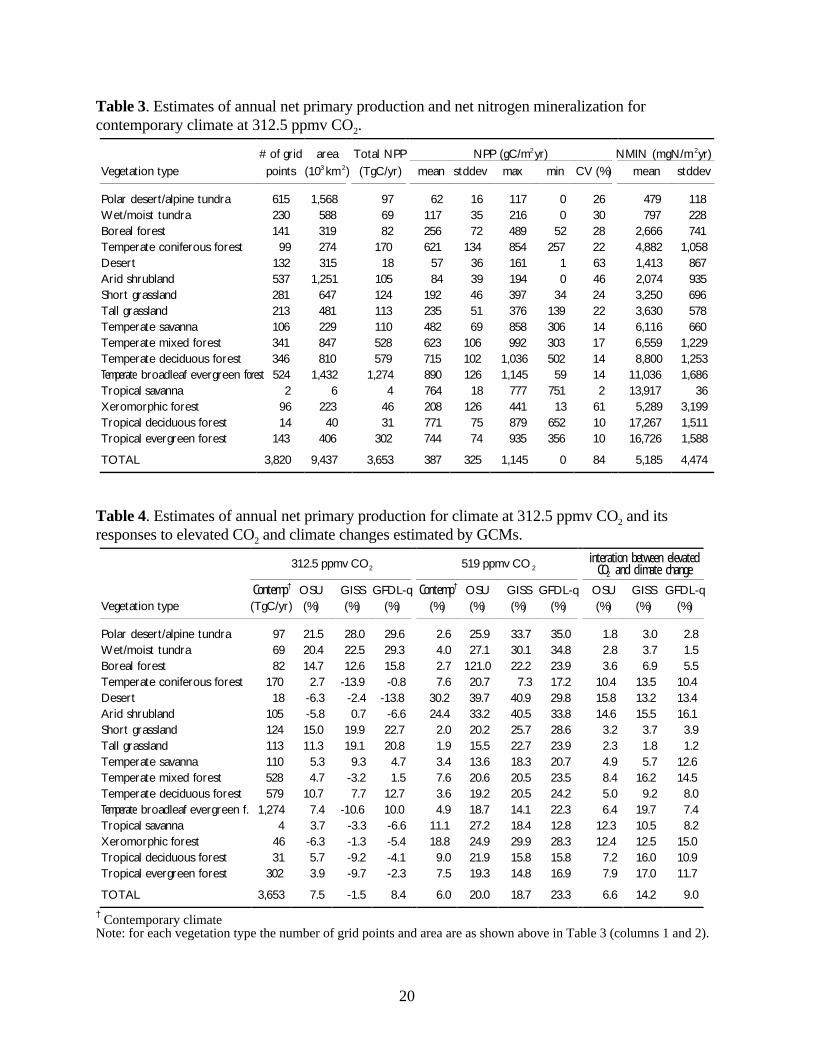
3. Net Primary Production Under Contemporary Climate at 312.5 ppmv CO2

At the continental scale, TEM estimated that total annual NPP of terrestrial ecosystems inChina for contemporary climate at 312.5 ppmv CO2 is 3,653 TgC yr-1 (1012 gC yr-1). Among the 16biomes, annual NPP for a biome ranges from 4 TgC yr-1 in tropical savanna to 1,274 TgC yr-1 intemperate broadleaf evergreen forest (Table 3). Temperate forests (temperate coniferous forest,mixed forest, deciduous forest and broadleaf evergreen forest) account for 71.1% of the totalannual NPP of China, but only cover about 35.6% of the total land area of China. Tropical forests(tropical deciduous forest and evergreen forest) occur over 4.7% of the total land area, and theirannual NPP accounts for 9.1% of the total annual NPP of China. Arid and semi-arid ecosystems(desert, shrubland, shortgrassland and tallgrassland) occur over 28.5% of the total land area, butonly account for 6.5% of the total annual NPP of China.

The relative importance of a biome to the total annual NPP of China reflects the relativeproductivity among biomes. Area-weighted mean biome NPP varies considerably among the 16biomes (Table 3). Desert has the lowest mean biome NPP of 57 gC m-2yr-1. In desert and aridshrublands, NPP is controlled primarily by water availability, where annual precipitation is only74 mm and 124 mm, respectively. In alpine desert/alpine tundra and wet/moist tundra, NPP iscontrolled primarily by low temperature, which results in a short plant growing season and low

8

nitrogen availability because of lower rate of net nitrogen (N) mineralization (NMIN). Temperatebroadleaf evergreen forest is the most productive biome with a mean biome NPP of 890 gCm-2yr-1. In general, NMIN is higher in warm temperate and tropical biomes, but lower in highlatitude and plateau biomes (Table 3). This indicates that mean biome NPP is closely related toannual net nitrogen mineralization rate in soils.

Spatial variation of NPP within a biome differs among the 16 biomes (Table 3). Desert has thelargest spatial variation in NPP with a coefficient of variation of 63%. In contrast, tropicaldeciduous forest and evergreen forest have small spatial variations in NPP with a coefficient ofvariation of 10%. Spatial variation of NPP within a biome is primarily determined by spatialvariations of climate. As shown in Table 2, spatial variations in temperature and precipitationwithin a biome are large and differ among the biomes. The coefficient of variation in annualprecipitation is large in desert, xeromorphic forest and arid shrubland, but small in tropical forests(Table 2).

At the scale of grid cell, annual NPP is significantly correlated with annual precipitation(Figure 2), annual mean temperature (Figure 3) and annual mean cloudiness (Figure 4). Annualprecipitation accounts for 60% of the total variation in annual NPP among the 3,820 pixels, annualmean temperature accounts for 52%, and annual mean cloudiness accounts for 52%, respectively.Annual precipitation (Pann) and annual mean temperature (Tann) together accounts for 70% of thetotal variation in annual NPP (NPP = 54.0 + 0.35 Pann + 1.76 Tann, r

2 = 0.70, p < 0.001). Annualprecipitation, annual mean temperature and annual mean cloudiness (Cann) together account for72% of the total variation in annual NPP (NPP = −127.1 + 0.26 Pann + 16.2 Tann + 5.2 Cann,r2 = 0.72, p < 0.001).

Geographically, annual NPP decreases from southeast to northwest (Plate 4a). SouthernChina has high annual NPP of more than 1,200 gC m-2yr-1. The spatial patterns of NPP arecorrelated with the spatial patterns of precipitation and temperature (Plate 3). Annual NPP inQinhai-Tibet Plateau is very low because of low temperature and the short plant growing season.Annual NPP in Xinjian, Ninxia and Inner Mongolia is also very low, because of the small amountof annual precipitation.

4. Equilibrium Responses of Net Primary Production to Changes in Climate and CO2

4.1 NPP response to climate change only

For climate change with 312.5 ppmv CO2, TEM estimates that the continental response ofannual NPP in China ranges from a decrease of 54.8 TgC yr-1 (−1.5%) for the GISS climate to anincrease of 306.9 TgC yr-1 (8.4%) for the GFDL-q climate (Table 4). These differences in NPPresponse are determined by the differences among the three GCM climates. According to theGCMs projections, changes in annual mean temperature in China ranges from an increase of2.9 ˚C for the OSU climate to an increase of 4.2 ˚C for the GISS climate (Table 5). Annualprecipitation increases considerably but varies little among the GCMs, i.e. 15.5% for the GFDL-q

9

climate to 17.6% for the GISS climate (Table 5). However, annual mean cloudiness declinesslightly, ranging from −0.2% for the OSU climate to −1.2% for the GFDL-q climate (Table 5).

In TEM, climate change affects NPP in a number of ways. Temperature change will affectplant photosynthesis. Elevated temperature will increase potential evapotranspiration (PET) andplant respiration. Higher PET will generally result in lower soil moisture, which enhances waterstress of plants. Higher plant respiration and stronger water stress of plants may reduce NPP.Elevated temperature will enhance decomposition of soil organic matter, which releases moremineralized N available for plant uptake. Enhanced uptake of N by plants may increase NPP. Anincrease of precipitation may increase soil moisture and thus alleviate water stress of plant, and italso enhances decomposition of soil organic matter. A decrease of cloudiness will increase amountof total solar radiation and photosynthetic active radiation (PAR) that reaches the canopy ofvegetation. Higher PAR may increase GPP and NPP. Higher total solar radiation will increasePET. As described earlier, higher PET may enhance water stress of plants, which leads to adecrease of GPP and NPP. At the biome scale, the response of annual NPP varies substantially within a GCM (Table 4).For the GISS climate, biome NPP ranges from a decrease of 13.9% in temperate coniferous forestto an increase of 28.0% in polar desert/alpine tundra. The TEM estimates that annual NPP intundra and boreal forest increase substantially for the three GCM climates, because all the GCMsproject large increases of temperature and precipitation in these biomes (Table 5). Elevatedtemperature in tundra and boreal regions will significantly prolong the plant growing season andincrease nutrient availability from enhanced decomposition of soil organic matter. Annual NPP forarid biomes (desert and arid shrubland) decreases moderately, except for arid shrubland in theGISS climate, in which there are large increases of annual precipitation and annual meancloudiness (Table 5). Annual NPP of tropical deciduous forest and evergreen forest increasesmoderately for the OSU climate but declines for both the GISS and GFDL-q climate. Theseresponses are attributable to the larger increases of annual precipitation and annual mean cloudinessas well as a smaller increase in annual mean temperature in the OSU climate (Table 5). The mostsignificant differences in annual NPP response among the GCM climates occur in temperatebroadleaf evergreen forest, i.e., −135 TgC yr-1 (−10.6%) for the GISS climate, 96 TgC yr-1

(7.5%) for the OSU climate and 107 TgC yr-1 (8.4%) for the GFDL-q climate. These differencescan be attributed to the substantial increase of annual mean temperature (4.8 ˚C), large decrease ofannual mean cloudiness (−10.9%) and slight decrease of annual precipitation (−1.2%) in the GISSclimate (Table 5). In contrast, both the GFDL-q and OSU project smaller increases in temperatureand larger increases in precipitation (Table 5).

The response of NPP to climate change has large regional variations within a GCM climate(Plate 4b). For the GISS climate, NPP decreases substantially in Southern China but increase inNortheastern China. In Southern China, the GISS GCM predicts the largest increase of annualmean temperature and a decrease of annual precipitation and annual mean cloudiness (Plate 3). Forthe three GCMs climate, annual NPP decreases less than 20 gC m-2yr-1 in the arid and semi-aridregions in the Northwestern China, including the Loess Plateau. The Qinhai-Tibet Plateau has an

10

increase of annual NPP less than 40 gC m-2yr-1. However, the geographical distribution of NPPresponse in Southern China varies considerably among the GCM climates (Plate 4b). In the GISSand OSU climates, annual NPP decreases significantly in the Chendu Plain in the ShichuanProvince, where is the most productive agricultural zone and the most dense settlement of humanpopulation. In contrast, annual NPP increases in the Chendu Plain for the GFDL climate.

4.2 NPP response to elevated CO2 only

For contemporary climate with elevated CO2 (519 ppmv), TEM estimated that annual NPPincreases by 219 TgC yr-1 (6.0%) in China. In TEM, a direct effect of elevated atmospheric CO2

level is to increase the intercellular CO2 concentration within the canopy, which potentiallyincreases GPP via a Michaelis-Menton (hyperbolic) function. Elevated atmospheric CO2 level mayalso indirectly affect GPP by altering the carbon-nitrogen status of the vegetation increase efforttoward nitrogen uptake; increased effort is generally realized only when GPP is limited more bycarbon availability than by nitrogen availability (VEMAP Members, 1995).

At the biome scale, annual NPP increases for all of the 16 biomes (Table 4). The NPPresponses vary substantially among biomes, ranging from an increase of 1.9% in tall grasslands toan increase of 30.2% in desert (Table 4). Biomes in the arid regions (desert, arid shrubland) havethe largest percentage increase in annual NPP. This is attributed mostly to a significant increase ofwater use efficiency of plants in the arid regions, where water is the primary limiting factor onNPP. Temperate forests and boreal forests are generally limited by the availability of inorganicnitrogen in the soils, and as the result, their responses to elevated CO2 is strongly constrained bynitrogen availability. Tropical savanna, xeromorphic forest, tropical deciduous forest and tropicalevergreen forest have large increases of annual NPP in the range of 7.5% to 18.8%. In the tropicalregions, annual NPP of ecosystems is generally not limited by nitrogen, because of high rates ofnet N mineralization resulting from high temperatures.

The geographical distribution of NPP responses to elevated CO2 has distinct spatial patterns(Plate 4c). Annual NPP increase from about 20 gC m-2yr-1 to 300 gC m-2yr-1 in SoutheasternChina. Annual NPP in arid regions increases in the range of 20 to 40 gC m-2yr-1. In the Qinhai-Tibet Plateau, the response of annual NPP is within ±20 gC m-2yr-1 (Plate 4c). Annual NPP in theQinhai-Tibet Plateau is primarily controlled by low temperature and constrained by low nutrientavailability.

4.3 NPP response to changes in climate and CO2

At the continental scale, annual NPP of China for climate change at 519 ppmv CO2 increasessubstantially but varies little among the GCM climates, ranging from 683 TgC yr-1 (18.7%) for theGISS climate to 851 TgC yr-1 (23.3%) for the GFDL-q climate. Annual NPP increasesconsiderably for all of the 16 biomes among the three GCM climates (Table 4). Drylandecosystems (desert, arid shrubland) have the largest percentage increases in annual NPP (morethan 30%). Annual NPP in tundra and boreal forest also increases substantially (more than 20%).

11

Although the percentage increases in annual NPP for temperate broadleaf evergreen forest aremoderate, this biome accounts for the largest portion of the increase of annual NPP in China:238.2 TgC yr-1 for the OSU climate, 179.6 TgC yr-1 for the GISS climate and 284.1 TgC yr-1 forthe GFDL-q climate.

Geographically, the responses of annual NPP decrease from southeast to northwest within aGCM climate (Plate 4d). The spatial patterns of NPP responses are generally similar among thethree GCM climates. Annual NPP has a slight increase (< 40 gC m-2yr-1) in the Qinhai-Tibetplateau and arid regions, a moderate increase (40 to 60 gC m-2yr-1) in grasslands, and a largeincrease (> 60 gC m-2yr-1) in forest regions (Plate 4d). Increases of annual NPP in forest regionsare the largest in the GFDL-q climate, up to 200–300 gC m-2yr-1 in the southern China. For theGISS climate, NPP decreases in scattered areas of the Southern China (Plate 4). There are slightdifferences in both the magnitude and spatial distributions of NPP responses in the transitionalzones between forests and grasslands among the three GCM climates (Plate 4).

It is important to note that at the continental scale, the response of NPP to climate change at519 ppmv CO2 is much larger than the sum of the NPP response to elevated CO2 only and the NPPresponse to climate change only (Table 4). For the OSU climate, the sum of the NPP response forclimate change at 315 ppmv CO2 (7.5%) and the NPP response for contemporary climate at 519ppmv CO2 (6.0%) is much lower than the 20.0% NPP response for climate change at 519 ppmvCO2; the difference is attributed to the interaction between climate change and elevated CO2.Similarly, the interaction between climate change and elevated CO2 contributes about 9.0% to theoverall response of NPP to climate change at 519 ppmv CO2 for the GFDL-q climate and 14.2%for the GISS climate. The interaction between elevated CO2 and climate change is primarily causedby enhanced plant nitrogen uptake and increasing availability of mineralized nitrogen and carbon(CO2) resources. These results show clearly that the interaction between elevated CO2 and climatechange contributes significantly to the overall equilibrium response of NPP to changes in climateand CO2 (Table 4).

The relative role of the interaction between elevated CO2 and climate change varies among the16 biomes, ranging from a large role in arid biomes (e.g., desert, arid shrubland) to a small role inalpine tundra (Table 4). The relative role of the interaction between elevated CO2 and climatechange also varies among the three GCMs climates (Table 4). This indicates that geographicaldistributions of climate changes projected by the GCMs affect the interaction between elevated CO2

and climate change at larger spatial scales.

5. Discussion

There are numerous field measurements of plant biomass and NPP for various ecosystems inChina, however, few studies have estimated the spatial distribution of NPP in China on largespatial scales. Zhang (1993) calculated annual NPP for 671 weather stations in China, using theChikugo model (Uchijima and Seino, 1985). Fang, et al., (1995) and Xiao, et al., (1996)estimated annual NPP in China in 1990, using Normalized Difference Vegetation Index (NDVI)

12

derived from remote sensing data of NOAA AVHRR. In our study, the TEM-estimated annualNPP of all the terrestrial ecosystems in China under contemporary climate at 312.5 ppmv CO2 is3,653 TgC yr-1, about 8% of global terrestrial NPP (see Melillo, et al., 1993). Application ofprocess-based ecosystem models such as TEM provides an important and useful tool to studyspatial patterns and dynamics of NPP in China, although NPP estimates can be improved with thecollection of additional field data and remote sensing data to further develop and validate ecosystemmodels.

The TEM results show that annual NPP in China has a large spatial variation. Thegeographical distribution of annual NPP in this study is similar to Zhang (1993) and Xiao, et al.(1996), characterized by a gradient of high NPP in southeastern China to low NPP in northwesternChina. The spatial patterns of NPP are closely correlated to the spatial distributions of abioticfactors, particularly climate. This indicates that the spatial representation of contemporary climateand other abiotic factors used in extrapolation of TEM for China may affect estimates of NPP. Inan earlier study that examines three alternative geo-referenced data sets of climate, solar radiationand soil texture in estimating NPP of the conterminous United States, Pan, et al. (1996a) foundthat NPP estimates of TEM are sensitive to variations in the input data, and the relative importanceof climate, soil texture and solar radiation to NPP estimates differs among the vegetation types.

The spatial input data used in this study are from our global data base and need to be updatedwith the new data available in China. For instance, the climate data used in this study are the long-term average values of weather records from about 300 weather stations in China (W. Cramer,personal communication). Leemans and Cramer (1990) compiled weather record data mainly forthe period of 1931–1960. Zhang (1993) calculated biotemperature and potential evapotranspirationusing long-term average data from about 671 weather stations in China. Using more weatherstations in the spatial interpolation will improve the spatial and temporal (seasonal) representationsof contemporary climate.

Major soils in Xinjian, Qinhai-Tibet plateau and Inner Mongolia have generally about 40 to70% of sand proportion in soil texture (Xiong and Li, 1987), which is higher than the 35 or 45%of sand proportion we used in this study to drive TEM (Plate 2). In arid and semi-arid regions,coarse texture soils, which allow deep infiltration of water, may have lower evaporation but highertranspiration rate than fine texture soils (Noy-Meir, 1973; Sala, et al., 1988). Primary productionis therefore higher in coarse texture soils than in fine texture soils in arid and semi-arid regions(Noy-Meir, 1973). In grasslands of the Central Plains of United States, aboveground productionincreases with coarser soil texture when annual precipitation is less than 370 mm, but decreaseswhen annual precipitation is greater than 370 mm (Sala, et al., 1988).

Therefore, to improve estimates of NPP in China, geographically referenced spatial data withbetter spatial-temporal representations are critically needed. Improved data set will allow ecosystemmodels such as TEM to make more realistic estimates of NPP for contemporary climate. As thecontemporary climate data sets are also used in generating a “future climate” for impact analyses ofclimate change, improved contemporary climate data sets are likely to reduce the uncertainty inestimating responses of NPP in China to climate change.

13

The TEM results show that NPP of terrestrial ecosystems in China is sensitive to changes inatmospheric CO2 concentration and climate as projected by the GCMs. These results are consistentwith an earlier study (Xiao, et al., 1995) that used the CENTURY ecosystem model (Parton, et al.,1993) at individual sites and showed that NPP in grasslands of Inner Mongolia of China issensitive to changes in climate and atmospheric CO2 concentration. The TEM results also show thatthe magnitude and spatial distribution of NPP responses vary considerably among the GCMsprojections. The largest uncertainty in the NPP response to climate change among the three GCMclimates occurs in Southern China. The uncertainty in NPP responses is related to the uncertaintyin the GCMs projections for future climate change.

There is a large uncertainty in the GCMs projections for future climate changes. A number ofGCMs are available (Mitchell, et al., 1990). Most GCMs project a similar range of global surfacetemperature increase, but they vary significantly in the spatial patterns of projected changes intemperature and precipitation. Zhang and Wang (1993) examined the simulation results for 1 ×CO2 and 2 × CO2 scenarios from the Community Climate Model (CCM) at the National Center forAtmospheric Research (NCAR) of the United States. Annual mean temperature in China increasesby 2.5–3.0 ˚C. There is a large spatial variation in changes of annual precipitation in China. Inparticular, the NCAR CCM predicts a considerable decrease (about 200 mm) of annualprecipitation in the semi-arid Loess Plateau, where serious soil-water erosion and land degradationoccur extensively.

Because of the very coarse spatial resolutions of GCMs, GCMs are generally poor inrepresenting regional climate change, especially in China, which has very complex topography andthe climate is dominated by summer monsoon. Monsoon climate is characterized by seasonaljumps, large interannual variability and abrupt changes on decade and longer time scales. There arestrong interactions between climate and ecosystems in the Asian monsoon region on various timescales (Fu, 1995a). For instance, the normalized difference vegetation index (NDVI) for southernChina varied significantly in the period of 1985–1990 (Fu, 1995a). The coupling of GCMs andmeso-scale climate models with detailed representations of topography and ecosystem dynamicsmay generate better spatial-temporal representations of climate change in China (Fu, 1995b).

In this study, we have not considered the responses of vegetation distribution to climatechange and elevated CO2. Climate change is likely to affect the spatial distribution of vegetation inChina (Zhang and Liu, 1993; Zhang and Song, 1993; Zhang, 1993; Wang and Zhao, 1995; Zhouand Zhang, 1996). Vegetation redistribution can affect regional estimates of NPP of terrestrialecosystems (VEMAP Members, 1995). How climate change and elevated CO2 affect vegetationdistribution in China and consequently NPP is discussed in another paper (Pan, et al., 1996b).

We used the potential vegetation of China in this study. Thus, we have not considered theeffects of land use and management on NPP in China. In the last several thousand years ofagricultural practice, a large portion of uplands has been converted to croplands. According to theVegetation Map of China (Hou, et al., 1982), the area of croplands is approximately 1.5 millionkm2, or about 15% of the total land area of China. Based on the Land Use Map of China at thescale of 1:1,000,000 (Wu, 1990), cultivated lands account for about 14.2% of the total land area of

14

China (Wu and Guo, 1994). Conversion of forests to croplands results in significant losses ofNPP and carbon storage (Houghton and Skole, 1990). Climate change is likely to have significantimpacts on physical geographical zones (Zhao, 1993) and agriculture in China (Wang, 1993; Gongand Hameed, 1993; Ohta, et al., 1995). This study provides a baseline for future studies toinvestigate the impacts of changes in land use and land cover on NPP and carbon storage of China.

In summary, this study demonstrates the usefulness of integrating a process-based ecosystemmodel with geo-referenced spatial data in China for examining the spatial patterns and dynamics ofnet primary production of terrestrial ecosystems. However, the analyses in this study are based onan equilibrium changes in climate and carbon fluxes of terrestrial ecosystems. The time course ofchanges in atmospheric CO2 concentration, climate, land use and anthropogenic nitrogendeposition from the last several centuries to next century have not been considered. We arebeginning to conduct transient simulations of TEM to track the path and magnitude of theresponses of NPP over time (Melillo, et al., 1996), but progress is hindered by a lack of bothhistorical and future data with better spatial-temporal representation on climate, land use and Ndeposition in China. As these data sets become available in the near future, we should be able toimprove the estimates of NPP and to better assess the effects of land use and climate changes onNPP of terrestrial ecosystems in China.

Acknowledgments

The study was supported by the National Aeronautics and Space Administration’s EarthObserving System (NAGW-2669), the Department of Energy’s National Institute for GlobalEnvironmental Change (No: 901214-HAR) and the Joint Program on Science and Policy of GlobalChange at the Massachusetts Institute of Technology (CE-S-462041).

References

Fang, Z., Q. Xiao, Y. Liu and R. Sheng, 1995, Monitoring of some surface properties in Chinaby NOAA AVHRR. In: “China Contributions to Global Change Studies,” D. Yu and H. Lin(eds.), Science Press, Beijing, p. 146–151.

FAO/CSRC/MBL (undated), Soil Map of the World, 1:5,000,000, Unesco, Paris, France.Digitization (0.5˚ resolution) by Complex Systems Research Center, University of NewHampshire, Durham, and modifications by Marine Biological Laboratory, Woods Hole, MA.

FAO/UNESCO, 1971, Soil Map of the World, 1:5,000,000, Unesco, Paris, France.Fu, C., 1995a, Dynamics of monsoon-driven ecosystem: Concept, preliminary evidence and

proposal for further research. In: “China Contributions to Global Change Studies,” D. Yu andH. Lin (eds.), Science Press, Beijing, p. 103–106.

Fu, C., 1995b, Simulation of summer monsoon in east China by high resolution regional climate-ecosystem model (RCEM), In: “China Contributions to Global Change Studies,” D. Yu andH. Lin (eds.), Science Press, Beijing, p. 142–145.

Gates, D.M., 1985, Global biospheric response to increasing atmospheric carbon dioxideconcentration. In: “Direct Effect of Increasing Carbon Dioxide on Vegetation,” B.R. Strainand J.D. Cure (eds.), DOE/ER-0238, United States Department of Energy, Washington D.C.,

15

p. 171–184.Gong, G., and S. Hameed, 1993, Identification of climatically sensitive agricultural zones of

China. In: “Climate Change and Its Impact,” Y. Zhang, P. Zhang, H. Zhang and Z. Lin(eds.), Meteorology Press, Beijing, p. 78–90. (in Chinese with English abstract)

Hansen, J., G. Russel, D. Rind, P. Stone, A. Lacis, S. Lebedeff, R. Ruedy and L. Travis, 1983,Efficient three dimensional global models for climate studies: Model I and II, MonthlyWeather Review, 111:609–662.

Hansen, J., A. Lacis, D. Rind, G. Russel, P. Stone, I. Fung, R. Ruedy and J. Lerner, 1984,Climate sensitivity: Analysis of feedback mechanisms. In: “Climate process and ClimateSensitivity,” J.E. Hansen and T. Takahashi (eds.), Geophysical Monograph 29, MauriceEwing series 5, American Geophysical Union, Washington, D.C., p. 130–163.

Hou, X. (ed.), 1982, Vegetation map of China, 2nd edition, Science Press, Beijing. (in Chinese)Houghton, R.A., and D.L. Skole, 1990, Changes in the global carbon cycle between 1700 and

1985. In: “The Earth as Transformed by Human Action,” B.L. Turner, et al. (eds.),Cambridge University Press, Cambridge, UK, p. 393–408.

IPCC (Intergovernmental Panel on Climate Change), 1995, Climate Change 1994: Radiativeforcing of climate change and an evaluation of the IPCC IS92 emission scenarios, CambridgeUniversity Press, New York, p. 196–197.

Jensen, M.E., and H.E. Haise, 1963, Estimating evapotranspiration from solar radiation, Journalof the Irrigation and Drainage Division, 4:15–41.

Kimball, B.A., 1975, Carbon dioxide and agricultural yield: An assemblage and analysis of 430prior observations, Agronomy Journal, 75:779–788.

Leemans, R., and W. P. Cramer, 1990, The IIASA climate database for land areas on a grid with0.5˚ resolution, WP-90-41, International Institute for Applied Systems Analysis, Laxenburg,Austria, 60 pp.

Manabe, S., and R.T. Wetherald, 1987, Large scale changes in soil wetness induced by anincrease in carbon dioxide, Journal of the Atmospheric Sciences, 44:1211–1235.

McGuire, A.D., J.M. Melillo, D.W. Kicklighter, Y. Pan, X. Xiao, J. Helfrich, B. Moore, III,C.J. Vorosmarty and A.L. Schloss, 1996, The role of the nitrogen cycle in the globalresponse of net primary production and carbon storage to doubled atmospheric carbondioxide, Global Biogeochemical Cycles (in review).

McGuire, A.D., J.M. Melillo, D.W. Kicklighter and L.A. Joyce, 1995, Equilibrium response ofsoil organic carbon to climate change: empirical and process-based estimates, Journal ofBiogeography, 22:785–796.

McGuire, A.D., L.A. Joyce, D.W. Kicklighter, J.M. Melillo, G. Esser and C.J. Vorosmarty,1993, Productivity response of climax temperate forests to elevated temperature and carbondioxide: A North America comparison between two global models, Climatic Change,24:287-310.

McGuire, A.D., J.M. Melillo, L.A. Joyce, D.W. Kicklighter, A.L. Grace, B. Moore, III andC.J. Vorosmarty, 1992, Interactions between carbon and nitrogen dynamics in estimating netprimary productivity for potential vegetation in North America, Global BiogeochemicalCycles, 6(2):101–124.

Melillo, J.M., I.C. Prentice, G.D. Farquhar, E.D. Schulze and O.E.Sala, 1996, Terrestrial bioticresponses to environmental change and feedback to climate. In: “IPCC Climate Change 1995:The Science of Climate Change,” Intergovernmental Panel on Climate Change, CambridgeUniversity Press, p. 445–481.

Melillo, J.M., 1994, Modeling land-atmospheric interaction: A short review. In: “Changes in LandUse and Land Cover: A Global Perspective,” W.B. Meyer and B.L. Turner (eds.),Cambridge University Press, p. 387–409.

16

Melillo, J.M., A.D. McGuire, D.W. Kicklighter, B. Moore, III, C.J. Vorosmarty andA.L. Schloss, 1993, Global climate change and terrestrial net primary production, Nature,363:234–240.

Mitchell, J.F.B., S. Manabe, V. Meleshko and T. Tokioka, 1990, Equilibrium climate change andits implications for the future. In: “Climate Change: The IPCC Scientific Assessment,”J.T. Houghton, G.J. Jenkins and J.J. Ephraums (eds.), Cambridge University Press, NewYork, p. 131–172.

NCAR/Navy, 1984, Global 10-minute elevation data. Digital tape available through NationalOceanic and Atmospheric Administration, National Geophysical Data Center, Boulder, CO.

Noy-Meir, I., 1973, Desert ecosystems: Environment and producers, Annual Review of Ecologyand Systematic, 4:25–51.

Ohta, S., Z. Uchijima and W. Oshima, 1995, Effect of 2 × CO2 climatic warming on watertemperature and agricultural potential in China, Journal of Biogeography, 22:649–655.

Pan, Y., A.D. McGuire, D.W. Kicklighter and J.M. Melillo, 1996a, The importance of climateand soils on estimates of net primary production: A sensitivity analysis with the TerrestrialEcosystem Model, Global Change Biology, 2:5–23.

Pan, Y., J.M. Melillo, D.W. Kicklighter, X. Xiao and A.D. McGuire, 1996b, Potential responseof net primary production in terrestrial ecosystems of China to climate change: A simulationstudy by Terrestrial Ecosystem Model coupled with vegetation redistribution, Journal ofBiogeography ( in preparation).

Parton, W.J., J.M.O. Scurlock, D.S. Ojima, T.G. Gilmanov, R.J. Scholes, Schimel,T.ÊKirchner, J.C. Menaut, T. Seastedt, T. Garcia Moya, A. Kamnalrut and J.I. Kinyamario,1993, Observation and modeling of biomass and soil organic matter dynamics for thegrassland biome worldwide, Global Biogeochemical Cycles, 7(4):785–809.

Prinn, R., H. Jacoby, A. Sokolov, C. Wang, X. Xiao, Z. Yang, R. Eckaus, P. Stone,D.ÊEllerman, J. Melillo, J. Fitzmaurice, D. Kicklighter, Y. Liu and G. Holian, 1996,Integrated global system model for climate policy analysis: I. Model framework and sensitivitystudies, Joint Program on the Science and Policy of Global Change, Report No. 7,Massachusetts Institute of Technology, Cambridge, MA, 76 pp.

Raich, J., W., E.B. Rastetter, J.M. Melillo, D.W. Kicklighter, P.A. Steudler, B.J. Peterson,A.L. Grace, B. Moore, III and C.J. Vorosmarty, 1991, Potential net primary productivity insouth America: Application of a global model, Ecological Applications, 1(4):399–429.

Sala, O.E., W.J. Parton, L.A. Joyce and W.K. Lauenroth, 1988, Primary production of thecentral grasslands region of the United States, Ecology, 69:40–45.

Uchijima, Z., and H. Seino, 1985, Agroclimatic evaluation of net primary productivity of naturalvegetations: (1) Chikugo model for evaluating net primary productivity, Journal ofAgricultural Meteorology, 40(4):343–352.

VEMAP Members, 1995, Vegetation/Ecosystem modeling and analysis project: Comparingbiogeography and biogeochemistry models in a continental-scale study of terrestrial ecosystemresponses to climate change and CO2 doubling, Global Biogeochemical Cycles, 9(4):407–437.

Vorosmarty, C.J., B. Moore, III, A.L. Grace, M.P. Gildea, J.M. Melillo, B.J. Peterson,E.B. Rastetter and P.A. Steudler, 1989, Continental scale models of water balance and fluvialtransport: an application to South America, Global Biogeochemical Cycles, 3(3):241–265.

Wang, B., 1993, How to deal with the problem of global warming. In: “Climate Change and ItsImpact,” Y. Zhang, P. Zhang, H. Zhang and Z. Lin (eds.), Meteorology Press, Beijing,p. 1-15. (in Chinese with English abstract)

Wang, F., and Z. Zhao, 1995, Impact of climate change on natural vegetation in China and itsimplication for agriculture, Journal of Biogeography, 22:657–664.

Wang, W., and Y. Zhang, 1993, The potential change of precipitation of China under the

17

condition of globe warming induced by CO2 doubling. In: “Climate Change and Its Impact,”Y. Zhang, P. Zhang, H. Zhang and Z. Lin (eds.), Meteorology Press, Beijing, p. 257–265.(in Chinese with English abstract)

Wetherald, R.T., and S. Manabe, 1988, Cloud feedback processes in a general circulation model,Journal of the Atmospheric Sciences, 45:1397–1415.

Willmott, C.J., M.R. Clinton and W.D. Philpot, 1985, Small-scale climate maps: A sensitivityanalysis of some common assumptions associated with grid-point interpolation andcontouring, The American Cartographer, 12:5–16.

Wilson, C.A., and J.F.B. Mitchell, 1987, A doubled CO2 climate sensitivity experiment with aglobal climate model including a simple ocean, J. Geophysical Res., 92(D11):13,315–13,343.

Wu, C., 1990, Land Use Map of China (1:1,000,000), Science Press, Beijing. (in Chinese)Wu, C., and H. Guo, 1994, Land Use of China, Science Press, Beijing, p. 90. (in Chinese)Xiao, X., D.S. Ojima, W.J. Parton, Z. Chen and D. Chen, 1995, Sensitivity of Inner Mongolia

grasslands to global climate change, Journal of Biogeography, 22:643–648.Xiao, X., D.W. Kicklighter, J.M. Melillo, A.D. McGuire, P.H. Stone and A.P. Sokolov, 1996a,

Linking a global terrestrial biogeochemistry model and a 2-dimensional climate model:Implications for the global carbon budget, Tellus (in press).

Xiao, X., J.M. Melillo, D.W. Kicklighter, A.D. McGuire, P.H. Stone and A.P. Sokolov, 1996b,The relative roles of changes in CO2 and climate to the equilibrium responses of net primaryproduction and carbon storage of the terrestrial biosphere, Global Change Biology (inreview).

Xiao, Q., W. Chen, Y. Sheng and L. Guo, 1996, Estimating the net primary productivity in Chinausing meteorological satellite data, Acta Botanica Sinica, 38(1):35–39. (in Chinese withEnglish abstract)

Xiong, Y., and Q. Li (eds.), 1987, Soils of China, Science Press, Beijing, p. 333. (in Chinese)Zhang, X., 1993, A vegetation-climate classification system for global change studies in China,

Quaternary Sciences, 2:157–169. (in Chinese with English abstract)Zhang, Y., and L. Liu, 1993, The potential impact of climate change on vegetation distribution in

Northwest China. In: “Climate Change and Its Impact,” Y. Zhang, P. Zhang, H. Zhang andZ. Lin (eds.), Meteorology Press, Beijing, p. 178–193. (in Chinese with English abstract)

Zhang, Y., and J. Song, 1993, The potential impact of climate change on the vegetation in theNortheast China, ibid, p. 194–204.

Zhang, Y., and W. Wang, 1993, The potential change of ground surface air temperature under thecondition of global warming induced by CO2 doubling, ibid, p. 248–255.

Zhao, M., 1993, Impact of climate change on physical geographical zones of China, ibid,p. 168-177.

Zhou, G., and X. Zhang, 1996, Study on climate-vegetation classification for global change inChina, Acta Botanica Sinica, 38(1):8–17. (in Chinese with English abstract)

18

19

Tables, Figures and Color Plates

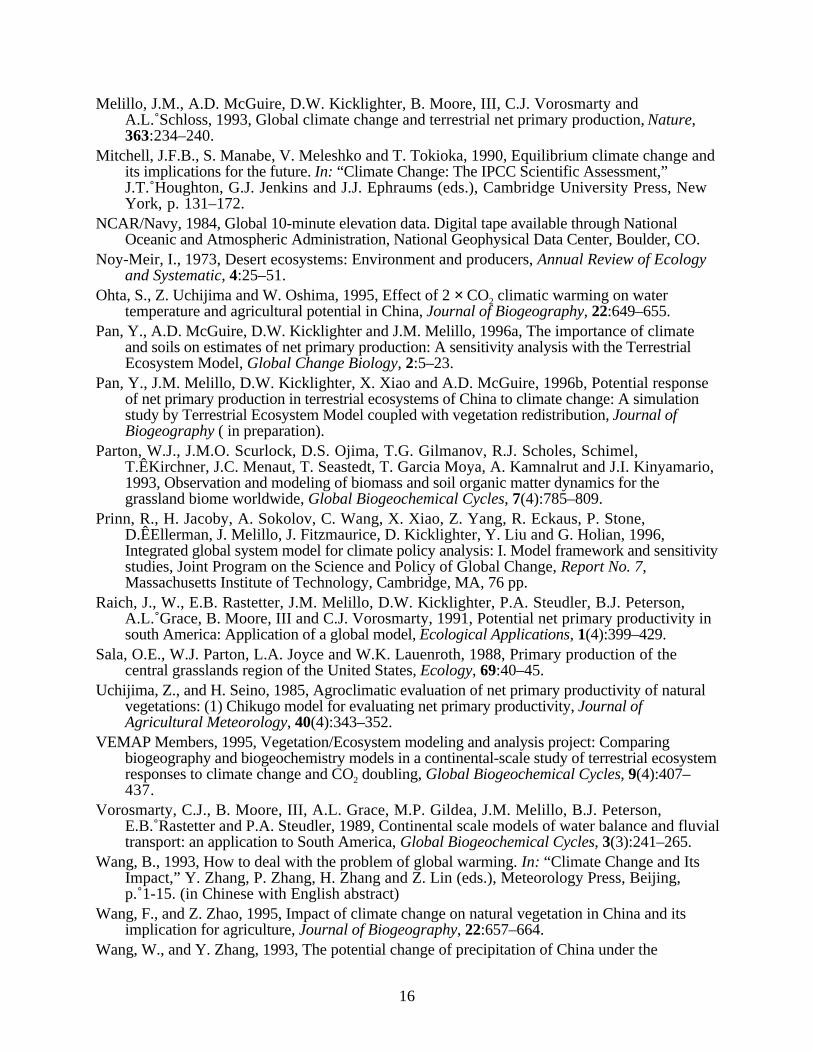
Table 1. Proportions of sand, silt and clay assigned to the FAO/CSRC/MBL soil texture class.

FAO/CSRC/MBL code Combination of FAO codes† Class description % sand % silt % clay

1 1 (coarse textured) sand 80 10 102 2 (medium textured) loam 45 40 153 3 (fine textured) clay 25 30 454 1 and 3 (coarse & fine) sandy loam 65 20 155 1 and 2 (coarse & medium) loam 45 40 156 2 and 3 (medium & fine) clay loam 35 30 357 1, 2, and 3 loam 45 40 158 none assigned to lithosols lithosols 45 40 15

† FAO codes: 1, coarse textured; 2, medium textured; 3, fine textured. No texture was assigned to lithosols.From Pan, et al., 1996.

Table 2. Means, standard deviations and coefficient of variations (CV) of annual meantemperature, annual precipitation and annual mean cloudines in contemporary climate.

# of grid area temperature (˚C) precipitation (mm) cloudiness (%)Vegetation type points (103 km2) mean stddev CV (%) mean stddev CV (%) mean stddev CV (%)

Polar desert/alpine tundra 615 1,568 -4.1 2.7 -66 480 316 66 43 5 11Wet/moist tundra 230 588 -2.4 2.9 -121 483 294 61 47 6 13Boreal forest 141 319 -0.3 5 -1667 643 278 43 52 7 14Temperate coniferous forest 99 274 13.2 4.7 36 1,249 384 31 63 6 10Desert 132 315 8.6 2.4 28 74 62 85 36 4 11Arid shrubland 537 1,251 6 3 50 124 106 86 37 5 12Short grassland 281 647 2.4 2.7 113 311 156 50 39 6 15Tall grassland 213 481 2.9 3.5 121 416 97 23 41 8 20Temperate savanna 106 229 3 2.2 73 550 141 26 40 5 12Temperate mixed forest 341 847 10.7 4.3 40 810 277 34 50 9 17Temperate deciduous forest 346 810 5.8 5.1 88 735 238 32 49 11 23Temperate broadleaf evergreen forest 524 1,432 14.7 2.6 18 1,320 269 20 69 6 9Tropical savanna 2 6 24.2 0.7 3 1,793 18 1 48 3 7Xeromorphic forest 96 223 6 3.2 53 243 167 69 36 4 11Tropical deciduous forest 14 40 19.7 3.3 17 1,350 341 25 57 7 12Tropical evergreen forest 143 406 19.4 3.7 19 1,590 374 23 61 7 11

TOTAL 3,820 9,437 5.8 7.6 131 661 493 75 48 13 26

20

Table 3. Estimates of annual net primary production and net nitrogen mineralization forcontemporary climate at 312.5 ppmv CO2.

# of grid area Total NPP NPP (gC/m2 yr) NMIN (mgN/m 2yr)Vegetation type points (103 km2) (TgC/yr) mean stddev max min CV (%) mean stddev

Polar desert/alpine tundra 615 1,568 97 62 16 117 0 26 479 118Wet/moist tundra 230 588 69 117 35 216 0 30 797 228Boreal forest 141 319 82 256 72 489 52 28 2,666 741Temperate coniferous forest 99 274 170 621 134 854 257 22 4,882 1,058Desert 132 315 18 57 36 161 1 63 1,413 867Arid shrubland 537 1,251 105 84 39 194 0 46 2,074 935Short grassland 281 647 124 192 46 397 34 24 3,250 696Tall grassland 213 481 113 235 51 376 139 22 3,630 578Temperate savanna 106 229 110 482 69 858 306 14 6,116 660Temperate mixed forest 341 847 528 623 106 992 303 17 6,559 1,229Temperate deciduous forest 346 810 579 715 102 1,036 502 14 8,800 1,253Temperate broadleaf evergreen forest 524 1,432 1,274 890 126 1,145 59 14 11,036 1,686Tropical savanna 2 6 4 764 18 777 751 2 13,917 36Xeromorphic forest 96 223 46 208 126 441 13 61 5,289 3,199Tropical deciduous forest 14 40 31 771 75 879 652 10 17,267 1,511Tropical evergreen forest 143 406 302 744 74 935 356 10 16,726 1,588

TOTAL 3,820 9,437 3,653 387 325 1,145 0 84 5,185 4,474

Table 4. Estimates of annual net primary production for climate at 312.5 ppmv CO2 and itsresponses to elevated CO2 and climate changes estimated by GCMs.

312.5 ppmv CO2 519 ppmv CO 2interation between elevatedCO2 and climate change

Contemp† OSU GISS GFDL-q Contemp† OSU GISS GFDL-q OSU GISS GFDL-qVegetation type (TgC/yr) (%) (%) (%) (%) (%) (%) (%) (%) (%) (%)

Polar desert/alpine tundra 97 21.5 28.0 29.6 2.6 25.9 33.7 35.0 1.8 3.0 2.8Wet/moist tundra 69 20.4 22.5 29.3 4.0 27.1 30.1 34.8 2.8 3.7 1.5Boreal forest 82 14.7 12.6 15.8 2.7 121.0 22.2 23.9 3.6 6.9 5.5Temperate coniferous forest 170 2.7 -13.9 -0.8 7.6 20.7 7.3 17.2 10.4 13.5 10.4Desert 18 -6.3 -2.4 -13.8 30.2 39.7 40.9 29.8 15.8 13.2 13.4Arid shrubland 105 -5.8 0.7 -6.6 24.4 33.2 40.5 33.8 14.6 15.5 16.1Short grassland 124 15.0 19.9 22.7 2.0 20.2 25.7 28.6 3.2 3.7 3.9Tall grassland 113 11.3 19.1 20.8 1.9 15.5 22.7 23.9 2.3 1.8 1.2Temperate savanna 110 5.3 9.3 4.7 3.4 13.6 18.3 20.7 4.9 5.7 12.6Temperate mixed forest 528 4.7 -3.2 1.5 7.6 20.6 20.5 23.5 8.4 16.2 14.5Temperate deciduous forest 579 10.7 7.7 12.7 3.6 19.2 20.5 24.2 5.0 9.2 8.0Temperate broadleaf evergreen f. 1,274 7.4 -10.6 10.0 4.9 18.7 14.1 22.3 6.4 19.7 7.4Tropical savanna 4 3.7 -3.3 -6.6 11.1 27.2 18.4 12.8 12.3 10.5 8.2Xeromorphic forest 46 -6.3 -1.3 -5.4 18.8 24.9 29.9 28.3 12.4 12.5 15.0Tropical deciduous forest 31 5.7 -9.2 -4.1 9.0 21.9 15.8 15.8 7.2 16.0 10.9Tropical evergreen forest 302 3.9 -9.7 -2.3 7.5 19.3 14.8 16.9 7.9 17.0 11.7

TOTAL 3,653 7.5 -1.5 8.4 6.0 20.0 18.7 23.3 6.6 14.2 9.0

† Contemporary climateNote: for each vegetation type the number of grid points and area are as shown above in Table 3 (columns 1 and 2).

21

Table 5. Means of changes in annual mean temperature (T), annual precipiation (P), and annualmean cloudiness (C), projected by GCMs.

# of grid area GISS GFDL-q OSUVegetation type points (103 km2) T (˚C) P (%) C (%) T (˚C) P (%) C (%) T (˚C) P (%) C (%)

Polar desert/alpine tundra 615 1,568 4.3 35.4 5.3 3.9 18.7 0.2 3.1 14.5 -1.9Wet/moist tundra 230 588 4 25.3 2.3 3.7 24.7 3 3.1 13.4 -1.7Boreal forest 141 319 4.1 11.5 -1.5 4.2 21.3 1.6 3.1 12.2 -1.4Temperate coniferous forest 99 274 4.6 -3.7 -9 3.6 10.2 -3.7 2.7 28.8 5.6Desert 132 315 4.4 25.7 3.8 4.2 8.1 -5.7 2.9 15.1 -1.4Arid shrubland 537 1,251 4.2 25.5 3.4 4.4 9.3 -4.5 2.9 11.7 -1.7Short grassland 281 647 4 15.1 -0.8 4.4 13.5 -2.6 2.9 9.3 -2.3Tall grassland 213 481 3.8 16.3 -1.3 4.6 16 -0.7 2.9 6 -3.3Temperate savanna 106 229 3.8 9.6 -1.9 5 16.6 -0.2 2.9 5.3 -3.3Temperate mixed forest 341 847 4 18.9 -2.2 4.4 18.6 2 2.8 12.4 -2.4Temperate deciduous forest 346 810 4 13 -3.2 4.5 21.4 2.3 2.8 10.3 -2.5Temperate broadleaf evergreen forest 524 1,432 4.8 -1.2 -10.9 3.9 15.4 -0.6 2.5 30.6 5.3Tropical savanna 2 6 3.4 24.4 4.8 3.1 0.6 -5.9 2.1 34.8 16.2Xeromorphic forest 96 223 4 18.8 0.1 4.4 13.6 -3.3 2.9 9.4 -2.7Tropical deciduous forest 14 40 4.1 10.6 -1.1 3.3 -4.8 -10.8 2.4 40.3 14.5Tropical evergreen forest 143 406 4 8.8 -4.6 3.5 1.7 -6.2 2.4 36.9 10.4

TOTAL 3,820 9,437 4.2 17.6 -1.2 4.1 15.5 -1 2.9 16.3 -0.2

NAV

NVLLN

RAGPP

NRESORB

NINPUT

NS

RH

CS

atmospheric carbon dioxide

NUPTAKEL

CV

NVS

LC

NMOBIL

NUPTAKES NETMINNLOST

vegetation soil

Figure 1. The Terrestrial Ecosystem Model (TEM). The state variables are: carbon in vegetation (CV);structural nitrogen in vegetation (NVS); labile nitrogen in vegetation (NVL); organic carbon in soils anddetritus (CS); organic nitrogen in soils and detritus (NS); and available soil inorganic nitrogen (NAV).Arrows show carbon and nitrogen fluxes: GPP, gross primary productivity; RA, autotrophicrespiration; RH, heterotrophic respiration; LC, litterfall carbon; LN, litterfall nitrogen; NUPTAKES, Nuptake into the structural N pool of the vegetation; NUPTAKEL, N uptake into the labile N pool ofthe vegetation; NRESORB, N resorption from dying tissue into the labile N pool of the vegetation;NMOBIL, N mobilized between the structural and labile N pools of the vegetation; NETNMIN, net Nmineralization of soil organic N; NINPUT, N inputs from the outside of the ecosystem; and NLOST,N loss from the ecosystem.