NET 222: COMMUNICATIONS AND NETWORKS FUNDAMENTALS ( NET 222: COMMUNICATIONS AND NETWORKS FUNDAMENTALS…

Networks and Communication Department

NET 222: COMMUNICATIONS AND NETWORKS FUNDAMENTALS (PRACTICAL PART)

Lab 2 : potting to Matlab

1


2

Lecture Contents Graph in MatLab 2-D plotting Creating and Type of graph Using Basic Plotting Functions Plotting Multiple graph in same plot Formatting plots Save ,Print ,Close and Export figure

3


Creating and Type of graph Using Basic Plotting Functions Plotting Multiple graph in same plot Formatting plots Save ,Print ,Close and Export figure

2-D plotting


4

Creating Graph in MATLAB

Command Description

Plot, plot3

Create 2-D graph and 3-D

plotyy 2-D line plots with y-axes on both left and right side

loglog Log-log scale plotfplot Plot function between specified limits

Line Plot Pie Charts, Bar Plots, and HistogramsComma

ndDescription

bar, bar3 Bar graph 2-D, 3-DPie, pie3 Pie graph 2-D, 3-D

hist Histogram plot

Discrete Graph Command Description

Stem, stem3 Plot discrete sequence data 2-D, 3-D

stairs Stairstep graph

5


Type of graph


6

POLTTING IN MATLAB Line plot FUNCTIONs:

Plot example:


7

POLTTING IN MATLAB Plot wit line specification example:


8

POLTTING IN MATLAB Plotyy ex:


9

POLTTING IN MATLAB Plot3 3D ex:


10

Pie Charts, Bar Plots, and Histograms

Bar & br3 ex:


11

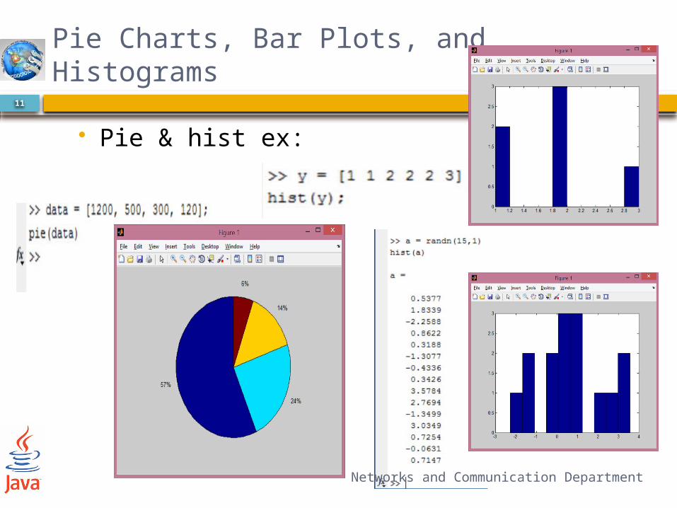
Pie Charts, Bar Plots, and Histograms

Pie & hist ex:


12

Discrete Graph Stem and stairs ex:

13


Plotting Functions

2-D PlottingSpecify x-data and/or y-dataSpecify color, line style and marker symbol(Default values used if ‘clm not specified)

Syntax: Plotting single line:

Plotting multiple lines:plot(x1, y1, 'clm1', x2, y2, 'clm2', ...)

plot(xdata, ydata, 'color_linestyle_marker')


15

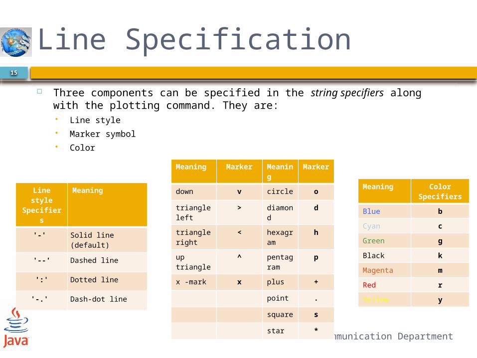
Line Specification Three components can be specified in the string specifiers along with the

plotting command. They are: Line style Marker symbol Color

Line style Specifiers

Meaning

'-' Solid line (default)

'--' Dashed line

':' Dotted line

'-.' Dash-dot line

Meaning Color Specifiers

Blue bCyan cGreen gBlack kMagenta mRed rYellow y

Meaning Marker Meaning

Marker

down v circle o

triangle left

< diamond

d

triangle right

> hexagram

h

up triangle

^ pentagram

p

x -mark x plus +

point .

square s

star *

2-D Plotting - exampleCreate a Blue Sine Wave» x = 0:.1:2*pi;» y = sin(x);» plot(x,y)

Basic Task: Plot the function sin(x) between 0≤x≤4π

Create an x-array of 100 samples between 0 and 4π.

Calculate sin(.) of the x-array

Plot the y-array

>>x=linspace(0,4*pi,100);

>>y=sin(x);

>>plot(y)0 10 20 30 40 50 60 70 80 90 100

-1

-0.8

-0.6

-0.4

-0.2

0

0.2

0.4

0.6

0.8

1

Adding a Grid GRID ON creates a

grid on the current figure

GRID OFF turns off the grid from the current figure

GRID toggles the grid state

»grid on

Controlling the Axes Setting Axis Limits & Grids

The axis command lets you to specify your own limits: axis([xmin xmax ymin ymax])

You can use the axis command to make the axes visible or invisible: axis on / axis off

The grid command toggles grid lines on and off: grid on / grid off


20

Using Basic Plotting Functions

Graphing functions MATLAB commandLabel the horizontal axis. xlabel('text')Label the vertical axis. ylabel('text')

Attach a title to the plot. title('text')Change the limits on the x and y

axis. axis([xmin xmax ymin ymax])"Keep plotting in the same

window." hold onTurn off the "keep-plotting-in-the-

same-window-command". hold off

using the strings to label various curves legend(‘string1’,’string2’,’s

tring3’)

Places the string (text) on the plot at coordinate x,y relative to the plot axes. text(x,y,’string’)

The following commands are useful when plotting:Note that all text must be put within ' '.

21


Multiple graph

Adding additional plots to a figure

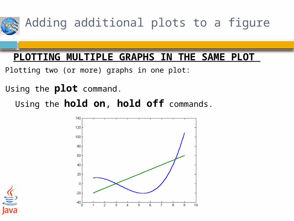
PLOTTING MULTIPLE GRAPHS IN THE SAME PLOT Plotting two (or more) graphs in one plot:

1. Using the plot command.

2. Using the hold on, hold off commands.

Adding additional plots to a figure

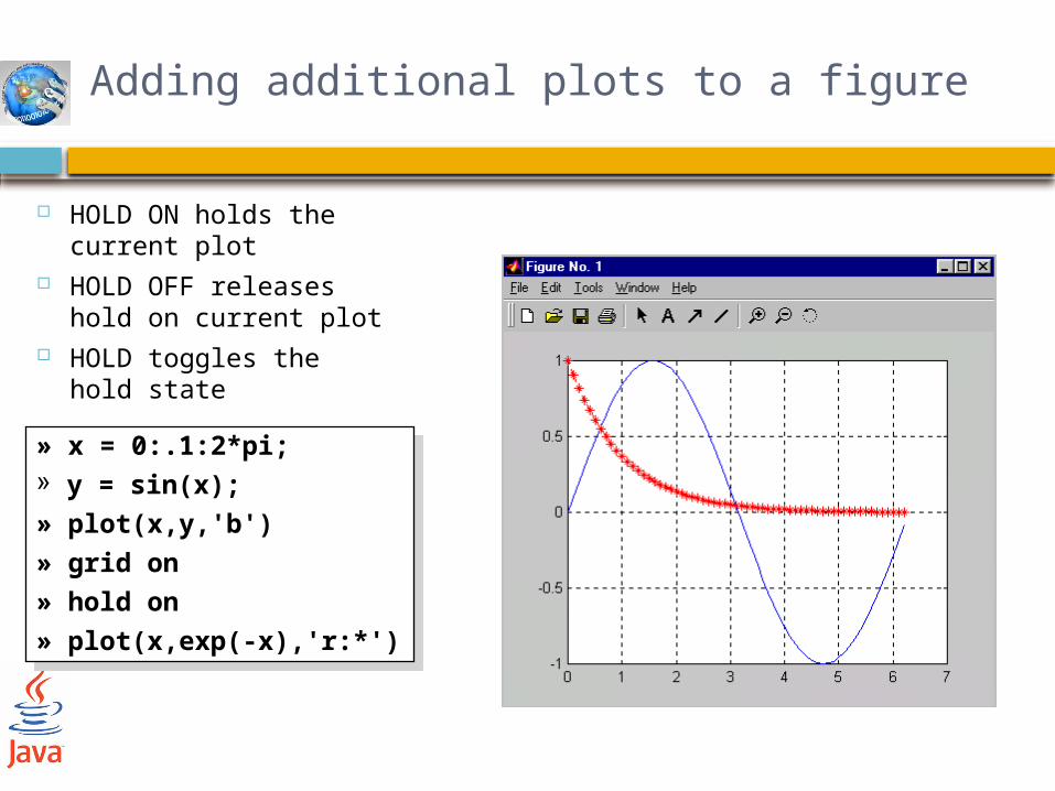
HOLD ON holds the current plot

HOLD OFF releases hold on current plot

HOLD toggles the hold state

» x = 0:.1:2*pi;» y = sin(x);» plot(x,y,'b')» grid on» hold on» plot(x,exp(-x),'r:*')


24

Subplots

25


Example Example 1: Plot sin(x) and cos(x) over [0,2π], on the same

plot with different colours Method 1:>> x = linspace(0,2*pi,1000);>> y = sin(x);>> z = cos(x);>> hold on;>> plot(x,y,‘b’);>> plot(x,z,‘g’);>> xlabel ‘X values’;>> ylabel ‘Y values’;>> title ‘Sample Plot’;>> legend (‘Y data’,‘Z data’);>> hold off;

26


Formatting

Formatting plots A plot can be formatted to have a required

appearance. With formatting you can:

Add title to the plot. Add labels to axes. Change range of the axes. Add legend. Add text blocks. Add grid.

Formatting plotsThere are two methods to format a plot:

1. Formatting commands.

In this method commands, that make changes or additions to the plot, are entered after the plot() command. This can be done in the Command Window, or as part of a program in a script file.

2. Formatting the plot interactively in the Figure Window.

In this method the plot is formatted by clicking on the plot and using the menu to make changes or add details.

Once a figure window is open, the figure can be formatted interactively.

Use Figure, Axes, and Current Object-Properties in the Edit menu

Click here to start the plot edit mode.

Use the insert menu to

FORMATTING A PLOT IN THE FIGURE WINDOW

30


Close and Save fig.

Close & Saving Plots You can close all the current plots using

‘close all’ Often you may want to save a plot to

include in another document, for example a Word document for a project report. From the figure window, save the plot in a file using the jpeg format. The jpeg format is pretty universal and compatible with MicroSoft Word and Powerpoint applications. It’s easy to do, give it a try.

Saving Figures

files extenstion:• .fig• also you can

save .jpeg .tif .bmp .pdf.

»plot3d_soln

using the Dialog Box:File Menu / Print... >>printdlg

from Command Line:

Controlling Page Layout:File Menu / Print Preview>>printpreview

Printing Figures

printprint('argument1','argument2',...)

Copying to Clipboard: Options: (Edit / Copy Option) Copying: (Edit / Copy Figure)

Exporting Figures

35


Any Questions ?The End

Documents

NET 222: COMMUNICATIONS AND NETWORKS FUNDAMENTALS ( NET 222: COMMUNICATIONS AND NETWORKS FUNDAMENTALS…