Nervousness in inventory management : comparison ofbasic control rulesde Kok, A.G.; Inderfurth, K.

Published in:European Journal of Operational Research

DOI:10.1016/S0377-2217(96)00255-X

Published: 01/01/1997

Document VersionPublisher’s PDF, also known as Version of Record (includes final page, issue and volume numbers)

Please check the document version of this publication:

• A submitted manuscript is the author's version of the article upon submission and before peer-review. There can be important differencesbetween the submitted version and the official published version of record. People interested in the research are advised to contact theauthor for the final version of the publication, or visit the DOI to the publisher's website.• The final author version and the galley proof are versions of the publication after peer review.• The final published version features the final layout of the paper including the volume, issue and page numbers.

Link to publication

Citation for published version (APA):Kok, de, A. G., & Inderfurth, K. (1997). Nervousness in inventory management : comparison of basic controlrules. European Journal of Operational Research, 103(1), 55-82. DOI: 10.1016/S0377-2217(96)00255-X

General rightsCopyright and moral rights for the publications made accessible in the public portal are retained by the authors and/or other copyright ownersand it is a condition of accessing publications that users recognise and abide by the legal requirements associated with these rights.

• Users may download and print one copy of any publication from the public portal for the purpose of private study or research. • You may not further distribute the material or use it for any profit-making activity or commercial gain • You may freely distribute the URL identifying the publication in the public portal ?

Take down policyIf you believe that this document breaches copyright please contact us providing details, and we will remove access to the work immediatelyand investigate your claim.

Download date: 03. Jun. 2018

E L S E V I E R European Journal of Operational Research 103 (1997) 55-82

EUROPEAN JOURNAL

OF OPERATIONAL RESEARCH

T h e o r y a n d M e t h o d o l o g y

Nervousness in inventory management: Comparison of basic control rules

T o n d e K o k a, K a r l I n d e r f u r t h b'* a Faculty of Technology Management, Eindhoven University of Technology, P.O. Box 513, 5600 MB Eindhoven, The Netherlands

b Faculty of Economics and Management, University of Magdeburg, P.O. Box 4120, D-39016 Magdeburg, Germany

Received 1 January 1996; accepted 1 August 1996

Abstract

Using a rolling horizon planning framework in inventory control leads to nervousness in the planning system caused by instability of order release decisions in successive planning cycles. For a single-stage inventory system with arbitrary stochastic demand it is shown analytically, how planning stability is affected by policy parameters if (s, nQ), (s, S), and (T,S) control rules are applied. It turns out that the reorder point s does not influence stability whereas the lot size determining parameters Q, S - s, and T can have a considerable impact. However, this influence turns out to be quite different for different measures of stability regarding order setup or order quantity deviations, respectively. Using these planning stability results the priority of the different control rules under the aspect of nervousness is discussed. (~) 1997 Elsevier Sciencc B.V.

Ke)~'ords: Nervousness; Planning stability; Rolling horizon planning; Inventory control rules

1. The nervousness problem in inventory management

Inventory management in a stochastic environment is usually based on simple control rules like reorder- level policies of the (s, nQ)- and (s, S)-type or like periodic order-up-to (T, S)-policies. These basic policies are simply to apply in practice in order to control inventory and replenishment processes in an uncertain environment. They are also widely investigated in inventory theory, especially considering the performance of their specific structure and dealing with the problem of optimal determination of their parameters.

In this context the performance of control rules is traditionally evaluated with respect to the costs they cause and, in case of avoiding estimation of shortage costs, with regard to the service degree they provide. Besides these two traditional pertormance measures in practice a third criterion can be of high importance. This is the level of planning stability that can be achieved in a rolling horizon planning framework.

The application of rolling horizons in inventory management is often found when inventory control rules are integrated in production planning where safety stocks and lot-sizing techniques are used to create a medium- term sequence of production and ordering decisions for a certain number of planning periods. This is done at

* E-mail: inderfurth@ww.uni-magdcburg.de; fax: +49-391 67 11168

0377-2217/97/$17.00 (E) 1997 Elsevier Science B.V. All rights reserved. PII S 0 3 7 7 - 2 2 17 ( 9 6 ) 0 0 2 5 5 - X

56 T. de Kok, K. lnderfurth/European Journal of Operational Research 103 (1997)55-82

the end-item level in master production scheduling (MPS level) as well as for all parts in a manufacturing system when a material requirements planning approach (MRP System) is used. In practice such planning is performed in a deterministic way replacing all stochastic inputs by appropriate quasi-deterministic forecasts. This means that the inventory control rules are also used with forecasted data as inputs. In an MRP context this procedure leads to what is called fixed order quantity (FOQ) planning or period order quantity (POQ) planning, respectively. Employing these planning rules can easily be shown to be identical to using inventory policies with fixed or variable lot sizes in a multi-period deterministic environment (cf. Lagodimos and Anderson, 1993).

Neglecting uncertainties facilitates multi-period planning, especially for a multi-level production system, but it evidently enforces the need for some kind of planning flexibility. This is necessary to allow for reacting on incoming information about the past (i.e. realizations of stochastic parameters) and the future (i.e. updated forecasts) in the dynamic planning process. The standard procedure of doing this is by periodically revising the actual plan while rolling forward the planning horizon. Now, in a stochastic environment this way of planning leads to continuous replanning activities due to the permanent integration of new information. These replanning operations are regularly connected with discontinuities in maintaining former ordering decisions known as the nervousness syndrome (see Vollmann et al., 1988). Nervousness or, in other words, lack of planning stability can turn out to be a significant problem because it often generates a considerable amount of short-run and medium-term adjustment efforts as well as a general loss of confidence in planning. Especially, in a multistage production environment ruled by an MRP system, nervousness on the top level (MPS-Ievel) is propagating throughout the system. Due to MRP time-phasing even future planning instability enforces present replanning actions. In many cases these consequences cannot be valued in terms of cost or lost profits, since relevant replanning expenses depend on time-varying availability of planning capacity, which can hardly be valued with respect to its contribution to a company's earnings. The same holds for the impairment of performance that short-term production control is facing due to quickly altering production decisions. Additionally, the loss of goodwill towards the planning system or the planning department generating a negative contribution to the behavior of people engaged in developing and executing production plans can never be expressed in money.

So it seems reasonable to treat planning stability as an independent attribute for assessing an inventory control system, similar to the attribute of costumer service which cannot be replaced by cost or protit values in most practical situations. For this reason we will not integrate the aspect of nervousness into pure cost-based inventory models like for instance in Kropp and Carlson (1984) and Krupp et al. (1983). Instead, we will treat planning stability as a specific criterion and investigate how it is affected by different inventory control rules. We note here that planning stability can be measured easily in practice as follows from the discussion below.

In order to evaluate these impacts, we have to define the phenomenon of planning stability more precisely (see Sridharan and LaForge, 1989; 1990). Undoubtedly, we face the most serious changes in the planning process when the actual order releases deviate from the planned orders that were determined in the previous planning cycle. Stability with respect to this dimension will be denoted by short-term planning stability. On the other hand, long-term stability considers the amount of planned order deviations in all periods of two consecutive planning cycles, including all prospective orders within the planning horizon. A further dimension of stability concerns the aspect of pure qualitative or quantitative changes of order decisions. A qualitative rcplanning action occurs if a planned production setup is canceled in a new planning cycle or if, vice versa, a new setup is planned. We denote stability with respect to this effect by setup-oriented stability. If deviations in the order quantities of successive planning cycles are of relevance for the performance of a planning system, we describe the respective criterion by quantity-oriented stability.

A general comparison of different control rules with respect to the dimensions of planning stability mentioned above is only possible if we use appropriate numerical stability measures. Unfortunately, up to now only little work has been done in developing and defining generally applicable measures of nervousness. In a wide set of simulation studies, which investigate the impact of different planning parameters on system nervousness, especially in MRP systems (cf. Blackburn et al., 1987; Minifie and Davis, 1990; Sridharan and Berry 1990; Yano and Carlson, 1987), only ad-hoc measures of nervousness are used. A systematic discussion and development

T. de Kok, K. Inderfurth/European Journal of Operational Research 103 (1997) 55-82 57

of stability measures is only found in Sridharan et al. (1988), Kadipasaoglu and Sridharan (1996), and in a more general way in Inderfurth (1994) and Jensen (1993; 1996). For assessing control rules in this study we use the measurement concept proposed in Jensen (1996) where nervousness is measured by the ratio of expected (quantity or setup) deviations of orders over the expectation of maximum deviations that can occur under worst case inventory control.

The simulation studies mentioned above don't give a precise and systematic insight into the dependence of nervousness on inventory control rules. In Jensen (1993; 1996) we lind a comprehensive investigation of reorder-point control rules which, yet, is limited in its informative value because it doesn't provide an analytical description of the interrelationship between control rules and planning stability. Analytical results of this type are presented in Inderfurth (1994) where, with respect to short-run stability performance, closed-form formulas are derived for the dependence of a setup-stability measure on the parameters of an (s, nQ ) and (s, S) inventory policy for uniform and exponential demand per period distributions. In our paper this analysis is extended to the quantity-stability situation, additionally incorporating more general demand distributions and also considering a reorder-cycle control rule.

The paper is organized as follows. In Section 2 the basic concept of a stationary investigation of nervousness is presented based upon a steady-state analysis of inventory control rules under a rolling horizon scheme. Section 3 contains analytical results of setup stability for all basic control rules, while Section 4 is dedicated to the analysis of quantity stability. Finally, in Section 5 some conclusions are drawn.

2. Steady-state analysis of planning stability

2.1. Inventory control problem

We restrict our analysis to a rolling horizon planning situation where a stationary inventory control rule for a single item is employed in a periodic review system. Every period we face a stochastic iid demand D with cdf Fo (.) The replenishment leadtime is without loss of generality assumed to be zero, unsatisfied demand is backlogged. In each planning cycle reorder decisions have to be made for an infinite planning horizon using demand forecasts/~t for period t which are assumed to be chosen equal to the demand expectation E[D] = b yielding constant forecasts for each period. Thus in each cycle an infinite sequence of planned orders is created which only differs from cycle to cycle if the initial inventory varies.

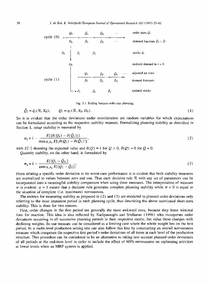
Denoting planned order sizes for a period t by Qt and planned (starting) inventories by ~t the development of the planning process consisting of two arbitrary consecutive planning cycles can be visualized like in Fig. 2.1 (cf. Sridharan and Berry, 1990).

In Fig. 2.1 the actual decision for the first period of each cycle is merely symbolized by Q0 and Ql indicating that this order will indeed be released whereas the others are still prospective. Considering short-term stability only a deviation between the planned and executed order for period 1 (Q1 and Ql) in both cycles does matter. From the replanning logic it can be realized that a deviation between Ql and Q1 only can occur if the actual stock Zl differs from its expectation ~l. This will happen when the initial demand Do as realization of the random variable D deviates from the demand forecast D.

2.2. Measures of planning stability

Due to stationarity of both the demand D and the applied control rule 7-¢, in steady-state the starting inventory Z0 is a stationary random variable with a cdfthat depends on 7-~ and Fo(.). The same holds for the inventory after replenishment X0 = Zo + Q0 which has a steady-state cdf denoted by Fx(.). Note that Q0 may be zero. Thus, for any replenishment policy also the order decisions are stochastic variables which can be written as follows:

58 Z de Kok, K. Inderfurth/ European Journal of Operational Research 103 (1997) 55-82

cycle (0) I

Do

Q0 Q! (.~2 " ' " order sizes Qt I I I i*

/30 D! /_32 ... demand forccasts/3t =/3

21 Z2 stocks Zt

re',.flized demand in t = 0

cycle ( 1 )

QI 02 03 "'" adjusted lot sizes I I I1~

DI /32 /33 demand fi~recasts

• Zl 2]2 23 updated stocks

Fig. 2.1. Rolling horizon order size planning.

01 =~1(7"¢,X0), QI =qI(TZ, Xo, Do). (1)

So it is evident that the order deviations under consideration are random variables for which expectations can be formulated according to the respective stability measure. Formalizing planning stabili ty as described in Section 1, setup stability is measured by

E [ ] 8 ( a l ) - 8 ( Q l ) [ I 7rs = 1 - , (2)

max. , ,% E[ J s ( a l ) - 8 ( Q I ) [ ]

with E [ . ] denoting the expected value and 8 ( Q ) = I for Q > 0, 8 ( Q ) = 0 for Q = 0. Quantity stability, on the other hand, is formulated by

E[IQI - Q,I] 'n'q = 1 - . (3)

maxTz,Fo El IOl - 01[]

From relating a specific order deviation to its worst-case performance it is evident that both stabili ty measures are normalized to values between zero and one. Thus each decision rule ~ with any set of parameters can be incorporated into a meaningful stability comparison when using these measures. The interpretation of measure 7r is evident: 7r = 1 means that a decision rule generates complete planning stability while ~- = 0 is equal to the situation o f complete (i.e. maximum) nervousness.

The metrics for measuring stability as proposed in (2) and (3) are restricted to planned order deviations only referring to the most imminent period in each planning cycle, thus describing the above mentioned short-term stability. This is done for two reasons.

First, order changes in the first period are generally the most awkward ones, because they leave minimal t ime for reaction. This idea is also reflected by Kadipasaoglu and Sridharan (1996) who incorporate order deviations occurring in all successive planning periods in their respective metric, but value these changes with declining weights. So our measure can be considered as a l imiting case where the whole weight lies on the first period. In a multi-level production setting one can also follow this line by constructing an overall nervousness measure which comprises the respective first per iod 's order deviations of all items at each level of the production structure. This procedure can be considered to be an alternative to taking into account planned order deviations of all per iods at the end-i tem level in order to include the effect of MPS-nervousness on replanning activities at lower levels when an MRP system is applied.

7£. de Kok, K. lnderfurth/European Journal of Operational Research 103 (1997) 55-82 59

The second reason for restricting considerations to short-term stability is the fact that our focus is on gaining analytical insight into the planning stability of production-inventory systems. This does not seem to be possible if a long-term stability measure including multiple period's order deviations is employed. However, as done by Jensen (1993; 1996), simulation can be used to investigate the impact of control rules on system nervousness under these circumstances.

A necessary condition for applying the stability measures defined in (2) and (3) is the determination of worst-case stability. For setup stability it is clear that maximum nervousness occurs under conditions where the first period's setup always differs from its previous expectation. This means that

max E[ I6 (QI ) - 6(01)1] = 1,

which along with (2) results in

7rs = 1 - E[ [6(Ql) - 6 ( 0 1 ) l ] - (4)

In other words, setup stability 7"rs can be described as the steady-state probability that 6 ( Q l ) will not deviate from the planned setup decision 6(01) ,

7rs = P{~(QI ) = 6(01) }. (5)

Determining the maximum quantity order deviation in (3) is a far more difficult problem, because there doesn't exist a natural upper limit for the quantity deviation of orders. It may be argued that in the long run the amount /9 has to be ordered per period allowing the deviations IQ1 - 011 in two consecutive cycle comparisons to be: 12t9 - 0l + ]0 - 2/9] = 4/9. Thus on the average a quantity deviation of 2/9 could be observed. This amount indeed can analytically be shown to be the maximum order deviation in the steady-state for a wide range of order rules and demand distributions. Nevertheless, as will be shown in a forthcoming paper, there exist extreme cases where the 2/9-limit can be exceeded.

As the 2/9-boundary is not violated for any parameter constellation of the basic control rules and demand distributions that are considered in this paper, we use this limit as maximum absolute order deviation in (3). So we get a quanti ty stabili ty measure as follows:

1 % = 1 - -~-~E[IQ1 - 01[]- (6)

With (5) and (6) the analysis of basic inventory control rules, with respect to the level of nervousness they may generate, concentrates on determining P { 6 ( Q 1 ) = 8(01)} and E[ [QI - Q l []. The value of these expressions will depend on the type of control rule under consideration, on the values of the control rule parameters, and on the demand distribution. Now, irrespective of the stochastic of demand some general results can be obtained.

2.3. General results f o r ( s, nQ) -po l i cy

Specifying inventory control rule ~ in (1) by an (s, nQ)-policy results in a planned order 0 as follows (omitting index "0" for notational simplicity):

{k. Q, for X - / 9 < s, 01 = 0, f o r X - D / > s , (7)

with

~= [s-X+b] -~ =k(s,Q,X).

60 T. de Kok, K. lnderfurth/European Journal of Operational Research 103 (1997)55-82

In the same way the actually executed first period's order is formulated as

k.Q, for X - D < s, QI = 0, forX-D>~s,

with

k= [ s - X + D]

From (7) and (8) we immediately find

I, for X - / ) < s, ~ ( 0 1 ) = 0, for X - / ) ~> s,

and

(8)

(9)

1, for X - D < s, 8(QI) = 0, f o r X - D ) s . (10)

Thus, from the definition of setup stability in (5), we get a stability measure

s-: D s+Q

rrs= / [ l - F l ) ( x - s ) ] d F x ( x ) + f Fo(x-s)dFx(x), (11)

S $:./)

where the cdf 's of demand (Fo( . ) as given) and stock after replenishment (Fx(.) to be determined) are used. By transformation of variables the ors-expression in ( 11 ) can be transformed to

Q Q-D

7rs= . / [1-Fo(Q-y)]dF~,(y)+ f Fo(Q-y) dF~,(y), (12)

Q-D 0

if we replace X by Y = s 4- Q - X. Here Y represents the difference between maximum and actual stock at the beginning of a steady-state period. Since for an (s, nQ)-policy X is restricted to s ~< X ~ s + Q, tbr Y holds: 0~<Y~<Q.

Now, from inventory theory (cf. Hadley and Whitin, 1963, pp. 245-248) we know that cdf F~,(.) does not depend on reorder point s. Thus, from (12) it follows that the setup stability for an (s, nQ) control rule only depends on the lotsize parameter Q.

It can be shown that the same is true for quantity stability. For evaluating (6), we have to determine E[IQI- 01[]. From (7) and (8), we find

E[[QI -Oil] = E [Ik(s,Q,X,D) -k(s,Q,X)l .Q], (13) D,X

Using the transformed variable Y, we can write (13) as

E[IQI - ~)11] = E [[k(Q,Y,D) - gz(Q,Y)I' Q] , (14) D,Y

with

k(Q,Y,D)= I Y - Q + D 1 and ~(Q,y)= [ Y - Q 4 - b ] • , Q "

With this result, we see that also quantity stability as defined in (3) does not depend on the value of the reorder point of an (s, nQ)-policy.

T. de Kok. K. lnderfurth/European Journal of Operational Research 103 (1997) 55-82 61

2.4. General results for (s, S) and (T, S)-policy

From the definition of an (s ,S) inventory control rule ~ , we find the order sizes in (1

and

S - X + / 3 , for X - / 5 < s, 01 = 0, f o r X - / ) >~s,

to be

15)

S - X + D, for X - D < s, 16) QI = O, for X - D ~ s.

Obviously, 8(01 ) and 6(Ql ) still are expressed by formulas (9) and (10). If we define the difference between reorder level S and reorder point s to be the mimmum lotsize Q i.e.

Q = S - s) setup stability for the ( s ,S ) rule can again be expressed by (4) or (5). As for (s, nQ) control it can be proved that the stability measures do not depend on the reorder level s.

Using Y= S - X , we can rewrite (15) and (16) as follows:

Ol = (Y+ff))l{y+l~>Q}, QI = ( Y + D)I{y+D>Q},

and thus

P{t~(Q1) = 8 (Qi )} = P{l{r+fg>a} = l{r+D>a}},

E[IQI - 0111 = E [ l ( Y + b ) l { v + b > a } -- (Y+D)I{r+O>Q}I] ,

which only depend on Q and not on s. A (T, S)-policy which is characterized by a fixed reorder cycle of length T and a reorder level S is simple to

analyze because in the first period of the cycle it is identical to an (s, S)-policy with S = s. For the other T - 1 periods of the replenishment cycle we have by definition: Q1 = Ql = 0. Thus, both setup and quantity stability will not depend on the order-up-to-level S while, in general, cycle length T will affect the planning stability. A special result turns out for setup stability if no zero demand can occur with positive probability. In this case it is evident that in each cycle one setup followed by T - 1 non-setups is planned as well as executed resulting in a 100% setup stability.

Summarizing, we can conclude that for reorder point policies the size of reorder point s does not influence the level of planning stability neither in the setup nor in the quantity direction. The reorder point only has an impact on the level of the inventory process but not on the deviations between planned and executed orders. Different from that it has been shown that lotsizing may have an impact on the magnitude of nervousness that is faced when a reorder point policy is employed. This influence will be analyzed in detail in the next sections.

3. Setup stabi l i ty for s imple inventory control rules

In this section we develop analytical expressions for the setup stability for the (s, nQ)-policy, (s, S)-policy and (T, S)-policy. The details of the analysis can be found in the appendices. In this section we restrict to the main results and a numerical comparison of setup stability for different demand distributions under different control rules. In the analysis we start from the general expressions for set-up stability as given in Section 2. In these expressions the probability distribution of Y plays a central role. We substitute the exact distribution of Y under the classical inventory control rules, which yields exact expressions for set-up stability. Further elaboration of these expressions enables the derivation of simpler exact expressions and practically useful approximations. In the sequel we assume that the demand per period is continuously distributed. The analysis for discrete demand distributions is quite similar.

62 T. de Kok, K. Inderfurth/European Journal of Operational Research 103 (1997) 55-82

3.1. ( s, nQ) -policy

For the (s, nQ)-policy we have that the pdf of Y is given by (cf. Hadley and Whitin, 1963, p. 257)

- Y for 0~<y ~< Q. P{Y <~ y } - Q,

Our starting point is Eq. (12). We distinguish between the cases Q > b and Q ~< D.

(17)

(i) Q <<, E). Substitution of (17) into (12) yields

a

'I "n ' s=~ ( l--Fo(Q--y))dy. 0

Hence it follows that

Q

'I ¢r~s'nQ) = ! - ~ Fo(y) dy.

0

(18)

(19)

(ii) Q > D. Substitution of (17) into (12) yields

Q-D Q , / 1/ 7"rs=~ Fo(Q - y) dy + ~ . ( l - - F D ( Q - - y ) ) d y .

0 Q-D

This finally yields straightforwardly

a Q

Q Q Fo(y) d y + Fo(y) dy.

o 15

(20)

Concluding, we find for (s, nQ)-policies

Q

77.~s,nQ)" -- 0 Q

° ': -~ FD(y) dy + -~ Fo(y) dy,

o D

for Q <~/5,

for Q > /9 .

(21)

Note that 7"1"~ s'nQ) is a continuous function of Q. Furthermore note that q.g~s,nQ) can be computed exactly for most tractable distributions.

T. de Kok, K. lnderfurth/ European Journal of Operational Research 103 (1997) 55-82 63

3.2. (s, S)-poli©'

For the (s, S)-policy we have that the pdf of Y is given by

M(y) O<~y<~Q, P{Y <<" Y} - M ( Q ) '

where the renewal function M(.) is defined as

M(y) = ~ F~*(y). n=0

(22)

(23)

Again we distinguish between the case of Q ~< O and Q > / ) , where Q = S - s.

(i) Q <~ if). applying (22), we find

7rs=P{Y + D > Q}= I - P{Y + D <<, Q} Q

1 fFo(Q - y) dM(y) . - 1 M(Q) 0

Since FD * M(y ) = M(y) - 1, we find

1 7r s = 1 - - ( M ( Q ) - 1).

M(Q)

Thus it follows that

1 .R-~ s,S) = M ( Q )

For the case of Q ~< D, we have that P{QI > 0} = 1. Substitution of this result into (12) and

(24)

(25)

(ii) Q >/5 . For the case of Q > D, we find from substitution of (22) into (12),

Q - D Q - y

1 / / d F o ( z ) d M ( y ) 7rs- M(Q) 0 0

a fyo

+ M(Q-~ Q-I ) Q - y

Q

+ M(O-------~ ( 1 - FD (Q - y) ) dM(y) .

Q-D

Q-D

_ 1 / FD(Q - y) dM(y) M(Q) .

0

This expression can be rewritten as

Q-D

~r'~s's)- l ~ { f F o ( Q - y ) d M ( y ) } . (26)

0

Both (25) and (26) are intractable in general, since tractable exact expressions for M(y) do not exist, except for special cases. In the appendix we give an exact expression for M(y) in case the demand is distributed

64 T. de Kok, K. Inderfurth/European Journal of Operational Research 103 (1997)55-82

according to a so-called K2-distribution. De Kok (1985) shows that the exact expression for M ( y ) in this case is given by

Y M ( y ) = l + ~ + y ( 1 - e - & ) , / : t ~ ]

y ) 0, (27)

for some constants y and /3. The rhs of (27) is proposed as a practically useful approximation for arbitrary renewal functions, when y and /3 are determined appropriately. In Appendix A expressions for Y and /3 are given. Summarizing, we have

{1 i M ( Q )

1 - M ( Q - L)) + 2

O-[

o

for Q ~</3,

for Q > / ) . (28)

In general rr~ s's) has a discontinuity at Q = /3 .

3.3. (T, S)-policy

As mentioned in Section 2.4 for the case of a (T, S)-policy it is easy to see that

~ s ) = 1. (29)

3.4. Comparison of control rules

It follows from (21) , (28) and (29) , that

~.~T.S) = 1 >~ "n'~ s'"Q) , ~.~T,S) ~> rr~s,s).

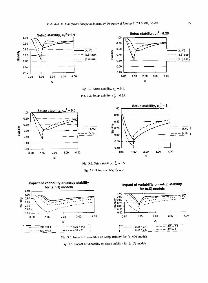
It is not clear which relation exists between 7r~ s'nQ) and rr~ s's) with identical Q = S - s. To obtain insight into this relation we have numerically compared rr~ s'nQ) and rr~ s's) for different values of Q and co, which is the coefficient of variation of D, i.e. cD = c r ( D ) / D . We have chosen /3 = 1.

We assumed Fo( . ) to be a mixture of two Erlang distributions (cf. Tijms, 1986, pp. 397-400) . Figs. 3.1-3.4 show the results of this comparison. For c~ = 0.1 and 0.25 (Figs. 3.1, 3.2) we have compared the exact expression for qT~ s'nQ), the approximation for rr~ s's) based on (27) and the "exact" value of ~.~s.S) derived from discrete event simulation. For c 2 >/ 0.5 (Figs. 3.3, 3.4), we compare the exact expressions for ~.~s,nQ) and rr~ ' 's). Furthermore note that the approximation for rr~ s's) is only valid for Q large ( Q / > 4/3, say). Another interesting observation is that 7r~ ' 's) shows local minima for Q = kD, k E N, when c 2 < 0.5. This can be explained by the fact that the inventory position has a probability mass at S and D is close to b with high probability when c~ small. As Q gets close to kD it may happen that either k periods or k + 1 periods occur between two orders of Q. This effect is apparently only visible for k = 1,2,3. If c2o /> 0.5 this effect has disappeared due to the high variations in D.

The following conclusions can be drawn. For Q < / 3 we have rr~ s'nO) /> rr~ s's), while for Q -~ 2D and larger Q-values we have rr~ s's) >~ rr~ ''"Q). In most practical situations the latter holds true, so that an (s, S)-policy should be preferred over an (s, nQ)-policy. On the other hand, under JIT conditions (i.e. Q <~ D ) , we find that an (s, nQ)-pol icy is advantageous with respect to the amount of planning stability it generates.

In Figs. 3.5, 3.6 we show the impact of demand variability on set-up stability. It is evident that the stability measure significantly deteriorates with increasing demand uncertainty.

T. de Kok, K. Inderfurth/European Journal of Operational Research 103 (1997)55-82 65

J~

&- =_ J ~

t / )

1.00

0.90

0.80

S e t u p s t a b i l i t y , CO 2 = 0.1 1.00

- - 0.80 \~, ] i (s,nQ) -,,

0.70 - - \ ~ = (s,S) appl ~=~ 0.70 ...... (s,S) sim j

0.60 . . >u 0.60 . - - , . _ _

0.50 I 0.50

0.40 I i ! 0.40 LO0 1.00 2.00 3.00 4.00 0.00

Q

Fig. 3.1. Setup stability, c~ = 0.1.

Fig. 3.2. Setup stability, ~o = 0.25.

S e t u p s t a b i l i t y , CO 2 = 0 . 2 5

- L - < s , n Q ,

il ..... <s,S) app - (s,S) sim

I I

1.00 2.00 3.00 4.00

Q

1.00

0.90

0.80

0.70

0.60

0.50

0.40 0.00

Setup stability, cD 2 = 0 . 5

-

1 i I 1.00 2.00 3.00 4.00

Q

1.00

0.90

0.80

I --~ 0.70 ~ ( s l n Q ) I ,

(s,S) 0.80

0.50

0.40

0.00

S e t u p s t a b i l i t y , CD 2 = 2

" ~ - i ; 1.00 2.00 3.00 4.00

Q

Fig. 3.3. Setup stability, c~o = 0.5.

(s,nQ)

(s,S)

Fig. 3.4. Setup stability, 3 D = 2.

I m p a c t o f v a r i a b i l i t y o n s e t u p s t a b i l i t y

f o r ( s , n Q ) m o d e l s

1.00 ~' 0.90 '~ 0.80

080. t \ ' v " ~''-" ,I 0.50 i i

0.00 1.00 2.00 3.00 4.00

I - ~ c D 2 = 0.1 . . . . . . cD2 = 0.5

I

Q

-- - - - - cD2 = 0.2 1 ! cD2 = 0.1 . . . . cD2 = 2 J I . . . . . . cD2 = 0.5

Fig. 3.5. Impact of variability on setup stability for (s, nQ) models.

Fig. 3.6. Impact of variability on setup stability for (s, S) models.

I m p a c t o f v a r i a b i l i t y o n s e t u p s t a b i l i t y

f o r ( s ,S ) m o d e l s

1.0o . ,, ~ J 0.90 Jr " - ~ ~ - - ~ . '~- ---° .'~" "~" "~" ]

• ~ 070 + ~ ' . ~ V - " " ~ - " ~ ~ -

~o.6o$ \ , : 0.50 ~ " ' . . . ' 0.40 | ~ I '

0.00 1.00 2.00 3.00 4.00

Q

- - - - - - cD2=0.2 I . . . . c D 2 = 2 j

6 6 T. de Kok, K. lnderfurth/European Journal of Operational Research 103 (1997)55-82

4. Quantity stability for simple inventory control rules

In Section 2 we introduced rrq as a measure for quantity stability. As in Section 3 we derive analytical expressions tbr rrq under (s, nQ)- , (s, S)- and (T, S)-policies. We provide tractable exact expressions for K2- distributions for the case of ( s, S) -policies and arbitrary demand distributions for the case of (s, nQ)- and (T, S)-policies. Tractable approximations are provided for arbitrary demand distributions under an (s, S)-policy.

4.1. ( s, nQ) -policy

As in Section 3.1 we distinguish between the cases Q ~< b and Q > D:

(i) Q <~ /3. expressions for QI and 21:

21 = { kQQ' f o r 0 ~ < Y ~ < ( 1 - w ) Q , ( k Q + I ) Q , f o r ( 1 - w ) Q < Y < ~ Q ,

Ql = { 0 , f o r Y < ~ Q - D , kQ, for kQ - D < Y <~ ( k + l )Q - D, k >~ l.

The integer function kQ is defined by

D = k Q Q + w Q , 0 ~ < w < 1.

From (14), we find

E[IQI - 21l] = E kQl{kQ<y+D<~(k+l)Q} -- kQQ - QI{(I_w)Q<y<~Q } . t., k=l

In Appendix B we show that after intricate algebra we find

t o

211] = 2 / ( 1 - F o ( y ) ) dy. E[ IO, * l

which is independent of Q!

From elaborating expression (1) in Section 2 for the case of Q ~< [), we find the following

(30)

(31)

(32)

(33)

(ii) Q >/3 .

Q I = { 0, kQ,

For the case Q > / 3 we have the following expressions for 21 and Ql:

for Y~< Q - b , f o r Q - D < Y < ~ Q ,

for Y <~ Q - D, f o r k Q - D <~ Y< ( k + I ) Q - D , k/> 1.

Note that we assumed that rcplenishment orders are triggered if the inventory position is below s. From (14) we derive the following expression for E[ IQl - 21l]:

E[[QI - 2 I l l = E kQl{kQ<~r+o<(k+l)Q} -- QI{Q_b<r<Q} . '-' k=-I

After cumbersome algebra, of which the major steps can be found in Appendix B, we find

(34)

(35)

T. de Kok, K. Inderfurth/European Journal of Operational Research 103 (1997) 55-82

O0

E[ [QI - 011] = 2 / ( l - FD (y) ) dy,

b

which is independent of Q and identical to (33)! Hence, we find that

- O I I ] = 2 f f l - F D ( y ) ) d Y , VQ. E[[Q1

Eq. (37) motivates the definition of ~-q as given in Section 2,

E[IQI -0111 7rq= l

215 '

since we find from (37) that

67

(36)

(37)

E [ I Q I - 011] ~< 2D,

whereby we have that 0 ~< ¢rq ~< 1. Hence, we conclude that

b (s,nQ) = 1 [ rrq ~ a ( 1 - Fo(y)) dy, (38)

0

where the superscript (s, nQ) emphasizes that this result holds for (s, nQ)-policies. Due to this strikingly simple result, we can obtain exact expressions for any tractable demand distribution used in practice.

4.2. ( s, S)-polic~y

As in Section 3.2 we derive exact analytical expressions for 7rq under an (s, S)-policy. We remark here that we do not obtain such an elegant result as in the case of an (s, nQ)-policy. Tractable exact expressions can only be given for K2-distributions, as was the case in Section 3.2. Again we distinguish between the cases Q < ~ / g a n d Q > D , w h e r e Q = S - s .

(i) Q ~D. For the case of Q ~ b , we expect a replenishmenteveryperiod. We lind the following expression

for Qj and 01:

Q1 = Y + / ) , Ql =(Y+D)I{y+D>Q}. (39)

Hence, we find

E[[Q1 - ~,{] = E[{(Y + D)l{r~o>Q} - Y - DII . (40)

In Appendix C we elaborate the expression on the rhs of (40) to obtain

Q

E[IQI-Oil] = 2 (1 - F D ( Y ) ) d Y + M(Q-----S b o

(41)

Comparison of (41) with (33) shows that

68 T. de Kok, K. lnderfurth/European Journal of Operational Research 103 (1997) 55-82

E(" '"Q)I[QI-0I l l <~ E~~'s)[IQ1- 0~I], Q~<D,

where the superscripts indicate the control rule applied. Hence, we find

~(s ,S ) "lT"(q s'nQ) /> , , q , for Q ~</5,

or, in other words, for Q ~< b the quantity stability of (s, nQ)-policies is greater than that of (s, S)-policies. In fact, any (s, nQ)-policy is more stable with respect to quantity stability than any (s, S)-policy with Q ~< D.

(ii) Q > D. For the case of Q > D, we find the following expressions Ibr Ql and Q1 (cf. (15) and

Ql = ( Y + D) l{r+b>a), Ql = ( Y + D)l{y+o>a}.

Hence, we find

E t [ Q , - 2 , 1 ] = E [ ] ( Y + D)I{v+~>Q)- (Y + D)I{r+O>Q}[ ] .

In Appendix C we elaborate the rhs of (43). This yields the following complicated exact expression E[ IQ I - QI [ ] :

16)):

(42)

(43)

~ r

Q Q-D c~

fb+YaM(y)-D+2ff 1-F°(z)dzaM(y)M(Q) M(Q) E[la~ - QI[] = Q - / 5 0 Q - y

Q-t)

+2Q / i-Fo(Q-y)M(Q) d M ( y ) + 2 M(Q) M(Q)-M(Q-ID)

0 f (1 - F o ( z ) ) d z .

h

(44)

The complete expression for 7r~ ''s) is found by inserting (41) and (44), respectively, into (6). Tractable exact expressions can only be found when D is K2-distributed because of the simple expression for M(-) in that case. Approximations can be derived along the lines sketched in Section 3.2.

4.3. (T, S)-policy

For the case of a (T, S)-policy we have to distinguish between periods in which we order and periods in which we do not order. Assume that at time 0 we just ordered such that the inventory position equals S at time 0, which is the beginning of period 1. Define

QI (t) := the actual order in period t,

Then it is easy to see that

T

1 ~--~EIIQI(t) - 01(t) l] . E[IQ - 0~I] = t=l

QI (t) := the planned order in period t.

(45)

By definition

Ol( t) = Ql( t ) = 0 , t = 2 . . . . . T.

Thus, we find

T. de Kok, K. lnderfurth/European Journal of Operational Research 103 (1997) 55-82 69

E[IQ~ - ~ 1 ] = 1 E [ I Q ~ ( I ) - {)~(1)11. (46)

{)l (1) and Qi (1) depend on the actual inventory position just before ordering at t ime 0. Because we order every T periods, we find

~)l(1) = D ( - T , - I ] + / ) , QI(1)=D(-T,O].

Thus, we find

E[]Q~ - {)~11 = E [ I D ( - I , 0 ] - bl] = E[ID - hi] /7) o¢~ oo

= / ( D - y ) d F o ( y ) + f (y-D)dFo(y)=2 f ( y -b )dFo(y) o D D

O 0

= 2 / ( 1 - FD(y)) dy.

This finally yields

O O

E[IQI - 011] = ~ ( D

and

1 - - F D ( y ) ) dy (47)

l/ TD (1 -Fo(y))dy. (48)

/3

Note the consistency between (48) , which holds for a (T,S)-policy, and (38) , which holds for an (s, nQ)- policy. Indeed, if T = 1 then both expressions on the rhs of (48) and (38) are identical, which is consistent with the fact that for T = 1 a (T,S)-pol icy is identical to an (s, nQ)-policy with Q ~ 0. From (38) and (48) we conclude that

rq( T,S 7.g~s,nQ), >~ V T,S,s,Q. (49)

Furthermore, it is obvious that for T = 1 a ( T, S) -policy is identical to an ( s ,S) -po l icy with s = S. From comparison of (41) and (48) it can be seen that in this case, of course, planning stability of both policies is equal.

4.4. Comparison of control rules

From the results obtained so far we can derive the following inequalities:

_(.~,s) Vs, S, T, for Q ~< D, .Tr(qT, S) ~ .ff~s,nQ) ~ n q ,

(T,S) > rr~S.,,Q), Vs, S, T, Q. qTq

We do not have an inequality for Q > L) w.r.t. (s , S)-policies in comparison with (s, nQ)-pol ic ies due to the intractability of (44) .

70 Z de Kok, K. lnderfurth/European Journal of Operational Research 103 (1997) 55-82

1.00

0.90

0.80

"~ 0.70

rn 0.60

0.50

0.40

0.00

J~

Quantity stabi l i ty , cn z = 0.1

1

2 N , ¢ : ' - . . . . _ . , ........ (s,nQ)

I (s,S) app J

I . . . . . . (s,S) sire '

I

1.00 2.00 3.00 4.00

Q

1.00

0.90

0.80

070

0.60

0.50

0.40

0.00

Q u a n t i t v stabi l i ty , c,, = = 0.5

- 1 i

I I I

1.00 2.00 3.00 4.00

1.00

0.90

0.80

"~ 0.70 u)

0.60

0.50 . . . . .

0.40

0.00

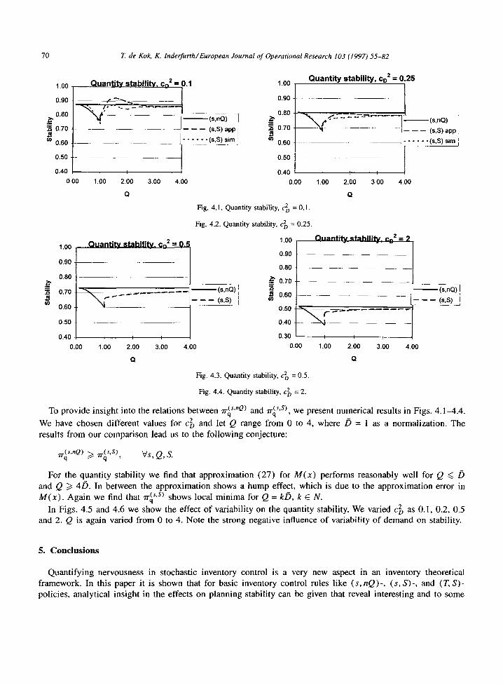
Fig. 4.1. Quantity stability,

Fig. 4.2. Quantity stability,

(s,n(~) I "~

(s,S) ]

Q u a n t i t y stabi l i ty , Co 2 = 0 .25

i . . . .

, tli 1.00 2.00 3.00 4.00

~2 D =0 .1 .

= 0.25.

1.00

0.90

0.80

0.70

0.60

0.50

0.40

0.30

0.00

O u a n t i t y . -~ tah i l i t y : c c 2 = 2

1.00 2.00 3.00 4.00

(s,nQ)

(s,S) app

- (s,S) sim

Q Q

Fig. 4.3. Quantity stability, C2D = 0.5.

Fig. 4.4. Quantity stability, ~o = 2.

~ ( s , n Q ) ! - - - (s,S) !

To provide insight into the relations b e t w e e n 7"l'(q s'nQ) and "rr (~'s)..q , we present numerical results in Figs. 4.1-4.4.

We have chosen different values for c2o and let Q range from 0 to 4, where /) = 1 as a normalization. The results from our comparison lead us to the following conjecture:

_(s.S) Vs, Q, S. 77"(q s'nQ) ~ ""q ,

For the quantity stability we find that approximation (27) for M(x) pertorms reasonably well for Q ~< b and Q >/413. In between the approximation shows a hump effect, which is due to the approximation error in M(x) . Again we find that 7r<q s's) shows local minima for Q = kD, k E N.

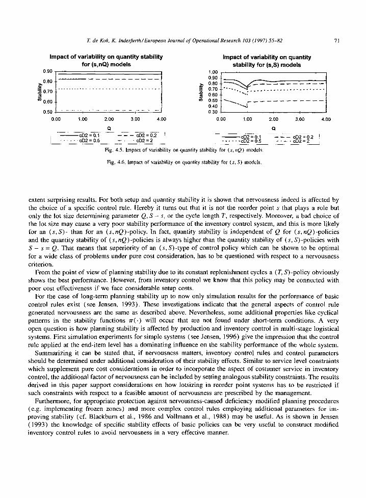
In Figs. 4.5 and 4.6 we show the effect o f variability on the quantity stability. We varied c~ as 0.1, 0.2, 0.5 and 2. Q is again varied from 0 to 4. Note the strong negative influence o f variability of demand on stability.

5. C o n c l u s i o n s

Quantifying nervousness in stochastic inventory control is a very new aspect in an inventory theoretical framework. In this paper it is shown that for basic inventory control rules like (s, nQ)-, (s, S)-, and (T, S)- policies, analytical insight in the effects on planning stability can be given that reveal interesting and to some

T. de Kok, K. lnderfurth/European Journal of Operational Research 103 (! 997) 55-82 71

Impact of variability on quantity stability for (s,nQ) models

0.90

--'~ 0 . 8 0

. . . . . . . . . . . . . . . . . • . . _ . . . . . . . _ . . . .

.o 0 . 7 0

¢n 0 . 6 0

0.50 . . . . . . . . . . . i . . . . . . . . . . . . . . . . . . . i . . . . . . . . . . .

0 . 0 0 1 . 0 0 2 . 0 0 3 . 0 0 4 . 0 0

(D

Q

- - c D 2 = 0.1 - - - - - - c D 2 = 0 . 2 J - - c D 2 = 0.1 . . . . _ _ - - c D 2 = 0 .5 . . . . - _ ' - - - - c D 2 = 2 j . . . . . . c D 2 = 0 .5

F i g . 4 . 5 . h n p a c t o f v a r i a b i l i t y o n q u a n t i t y s t a b i l i t y f o r ( s , nQ) m o d e l s .

Fig. 4.6. I m p a c t o f var iabi l i ty on quan t i ty stabil i ty for ( s , S) mode l s .

Impact of variability on quantity stability for (s,S) models

1 . 0 0 ,

. . . . . . . . . . .

0 . 6 0 ÷ " ' , /

o.5o i ~--'--....z- . . . . . . . . . . . . . . . . .

,

0.00 1.00 2.00 3.00

Q

- - - - - - c 0 2 = 0 . 2

. . . . c D 2 = 2

4.00

J

extent surprising results. For both setup and quantity stability it is shown that nervousness indeed is affected by the choice of a specific control rule. Hereby it turns out that it is not the reorder point s that plays a role but only the lot size determining parameter Q, S - s, or the cycle length T, respectively. Moreover, a bad choice of the lot size may cause a very poor stability performance of the inventory control system, and this is more likely for an (s, S)- than for an (s, nQ)-policy. In fact, quantity stability is independent of Q for (s, nQ)-policies and the quantity stability of (s, nQ)-policies is always higher than the quantity stability of (s, S)-policies with S - s = Q. That means that superiority of an (s, S)-type of control policy which can be shown to be optimal for a wide class of problems under pure cost consideration, has to be questioned with respect to a nervousness criterion.

From the point of view of planning stability due to its constant replenishment cycles a (T, S)-policy obviously shows the best performance. However, from inventory control we know that this policy may be connected with poor cost effectiveness if we face considerable setup costs.

For the case of long-term planning stability up to now only simulation results for the performance of basic control rules exist (see Jensen, 1993). These investigations indicate that the general aspects of control rule generated nervousness are the same as described above. Nevertheless, some additional properties like cyclical patterns in the stability functions ~r(.) will occur that are not found under short-term conditions. A very open question is how planning stability is affected by production and inventory control in multi-stage logistical systems. First simulation experiments for simple systems (see Jensen, 1996) give the impression that the control rule applied at the end-item level has a dominating influence on the stability performance of the whole system.

Summarizing it can be stated that, if nervousness matters, inventory control rules and control parameters should be determined under additional consideration of their stability effects. Similar to service level constraints which supplement pure cost considerations in order to incorporate the aspect of costumer service in inventory control, the additional factor of nervousness can be included by setting analogous stability constraints. The results derived in this paper support considerations on how lotsizing in reorder point systems has to be restricted if such constraints with respect to a feasible amount of nervousness are prescribed by the management.

Furthermore, for appropriate protection against nervousness-caused deficiency modified planning procedures (e.g. implementing frozen zones) and more complex control rules employing additional parameters for im- proving stability (cf. Blackburn et al., 1986 and Vollmann et al., 1988) may be useful. As is shown in Jensen (1993) the knowledge of specific stability effects of basic policies can be very useful to construct modified inventory control rules to avoid nervousness in a very effective manner.

72 Z de Kok, K. lnderfurth/European Journal of Operational Research 103 (1997) 55-82

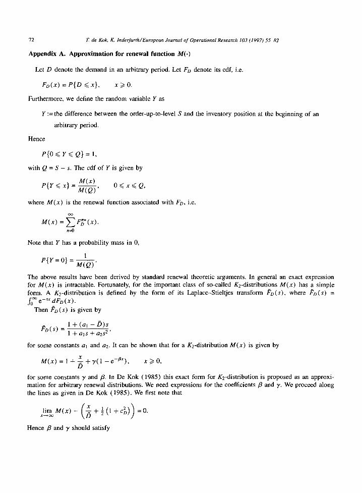
Appendix A. Approximation for renewal function M(-)

Let D denote the demand in an arbitrary period. Let Fo denote its cdf, i.e.

Fo(x) = P{D <~ x}, x >~ O.

Furthermore, we define the random variable Y as

Y := the difference between the order-up-to-level S and the inventory position at the beginning of an

arbitrary period.

Hence

e { o ~< Y ~< Q} = I,

with Q = S - s. The cdf of Y is given by

P{Y <~ x} = M(x) M ( Q ) ' O<~ x<~Q,

where M ( x ) is the renewal function associated with FD, i.e.

O O

F"* M(x) =/__, o (x) . n=O

Note that Y has a probability mass in 0,

1 P{Y = O} = M(Q)"

The above results have been derived by standard renewal theoretic arguments. In general an exact expression for M(x) is intractable. Fortunately, for the important class of so-called Kz-distributions M(x) has a simple form. A K2-distribution is defined by the form of its Laplace-Stieltjes transform ~'o(s), where FD(s) =

f o e-SX dFo(x) . Then Fo(s) is given by

1 + (al - / ) ) s P o ( s ) =

1 + a l s + a 2 s 2'

for some constants al and a2. It can be shown that for a K2-distribution M(x) is given by

M(x) = 1 + D + y(1 - e-aX), x ) O,

for some constants y and /3. In De Kok (1985) this exact form for K2-distribution is proposed as an approxi- mation for arbitrary renewal distributions. We need expressions/ 'or the coefficients/3 and y. We proceed along the lines as given in De Kok (1985). We first note that

xlimooM(x) - ( D + 21-(1 + c 2 ) ) = 0 .

Hence fl and y should satisfy

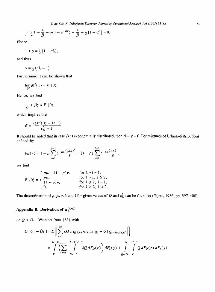
T. de Kok, K. lnderfurth/European Journal of Operational Research 103 (1997) 55-82

lim l + ~ + 3 / ( l - e -/~x) x--,~ D

x 1(1+C2o) =0 . D 2

Hence

73

1 + r = (1

and thus

Furthermore it can be shown that

l i m M ' ( x ) = F ' ( 0 ) . xl0

Hence, we find

1 -= + fly = F ' (O) , D

which implies that

2 ( F ' ( 0 ) - / ~ - i )

/ ~ = c~ - !

It should be noted that in case D is exponentially distributed, then fl = 3' = 0. For mixtures of Erlang-distributions defined by

k - I 1-1

FD(X) = 1 - - p ~ e-lZx(]Zx)i~. (1 - p ) ~--~C -vx(vx)ii! ' i=O i=O

we find

p / x + ( 1 - p ) v , f o r k = l = l , p/z, f o r k = l , 1/>2,

F ' ( 0 ) = (1 - p ) v , for k/> 2, / = 1 ,

0, for k/> 2, l />2 .

The determination of p,/.t, v, k and l for given values o f / ) and c2o can be found in (Tijms, 1986, pp. 397400 ) .

Appendix B. Derivation of "ri'(q s'nQ)

A: Q > / ) . We start from (35) with

E[ IQI - Qll] =E[ ~ kQI{kQ<~Y+D<(k+I)Q} - QI {Q_b<y<~Q} ] L, k=-I

Q-D (k+l)Q-y Q Q-y cg2

f (~-I f kQdFD(Z))dFy(y)+ f : QdFD(z)dFr(y) 0 kQ-y Q-D 0

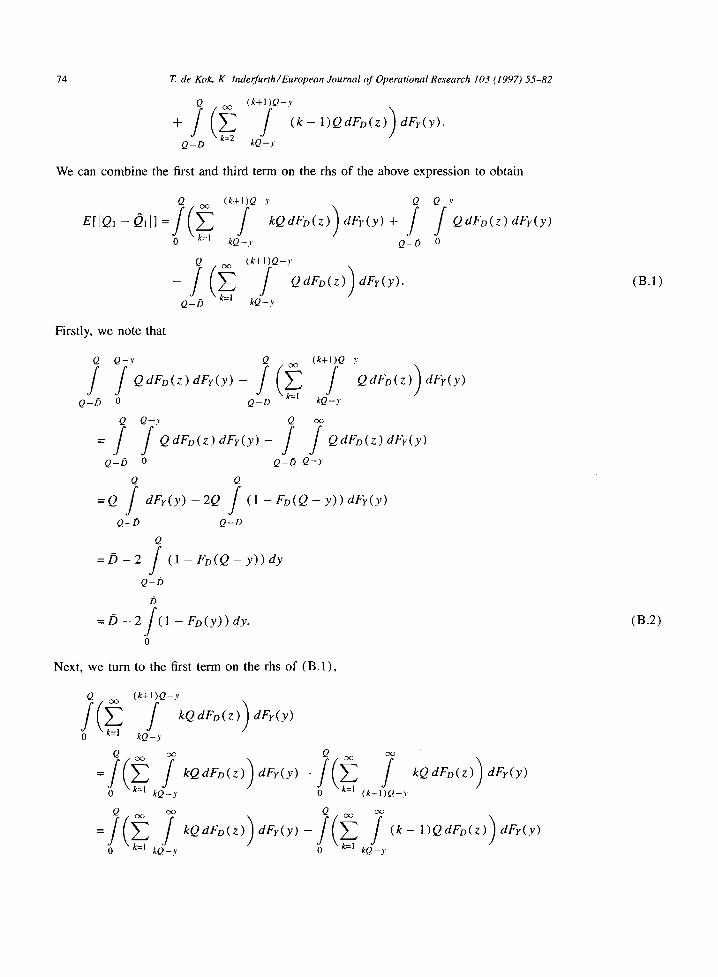
74 T. de Kok, K. lnderfurth/European Journal of Operational Research 103 (1997) 55-82

Q (k+l)Q-y

Q - D kQ-y We can combine the first and third term on the rhs of the above expression to obtain

Q (k-t-I)Q-y Q

oS( s ) EIIQ~ - 0,1] = k Q d F o ( z ) dFr(y ) +

kQ - y a _ f)

Q (k+l)Q-y

- f (D S QdFD(Z))dFy(y). Q-D kO-y

a - y

i QdFD(Z) dFr(y) 0

(B.1)

Firstly, we note that

Q Q - v Q - o o

i a-b o a-o

Q Q - y Q

(k+l)Q-y

i QdFD(z))dFy(y) k Q - y

i QdFt)(z) dFr(y) Q_/) 0 Q-/5 Q-y

Q Q

=Q S dFv(y)-2Q f (I-Fo(Q-y))dFr(Y) Q - D Q - D

Q

=/3-2 i (1-Fo(Q-y))dy Q-D

= / 3 - 2f(1 - FD(y)) dy. 0

(B.2)

Next, we turn to the first term on the rhs of ( B . I ) ,

Q (k+l)Q-y

o kQ-y

- ( - ) Q - . 0 - k Q - y 0 k 1

Q o o ~ Q oo oo

= / ( ~-~10 kj, kQdF°(z))dFY(y)-S(~-lo - kQ-vS (k-l)QdFD(z))dFr(y) - - _ , °

T. de Kok, K. hzderfurth/European Journal of Operational Research 103 (1997) 55-82

Q cx~

=p_ f / dFD(z)dFy(y) 0 k=-I k{~-y

oo Q f<l - F o ( k Q - y ) ) d y k=l 0

kQ OQ

= Z f ( I - F D ( z ) ) d z #=-1 (k-I)Q

=if).

Combining (B . I ) , (B.2) and (B.3), we obtain

b

E[IQt - 0,11 = 2 D - 2f(1 - Fo(y)) dy 0

= 2 . / ( 1 - Fo(y)) dy,

b

which is (36) .

B: Q <~ D. S i n c e Q ~ < / ) , w e c a n w r i t e b a s follows:

[) = kQQ + wQ,

It is easy

01=

Similarly,

a l =

Using (32) and the definitions of w and kQ, we find

(1 -w)Q Q - y

E[IQ,--011] = / f kQQdFD(z)dF},(y)+

0 ~ < w < ~ l , kQ E N.

to see that Q1 is determined as follows:

kQQ, for 0 ~< Y ~< (1 -w)Q, (kQ+I)Q, for (1-w)Q<~Y<Q.

we find for QI the following expression:

0, forO~ Y + D ~ Q, kO, for kQ <~ g + D <~ ( k + l )Q, k >/ l.

0 0

( I - w ) Q oo

0 k=l

Q O(3

+ f 2 ( I - w ) Q k=l

(1-w)Q

( k + l ) Q - y

f ]kQ - koQ I dFo(z) dFy(y) kQ-y

(k4 I ) Q - y

f IkQ- (ka+ l)OldFo(z)dFv(y). kQ-y

Q Q-y

f f ( k a + l ) Q d F o ( z ) d F v ( y )

o

75

(B.3)

(B.4)

(B.5)

76 T. de Kok, K. lnderfurth/European Journal of Operational Research 103 (1997) 55-82

The summations on the rhs of (B.5) can be elaborated analogously as we did for the case of Q > D. We give details for the first summation:

( l - w ) Q ( k + l ) Q - y

f ~-'~ i [kQ - kQQldFD(z) dFy(y) 0 k=l k Q - y

( I - w ) Q kO ( k ~ - l ) Q - y

= f ~ f (kQ-k)QdFD(z)dFl,(y) 0 k=l k Q - y

( l - w ) Q ( k + l ) Q - y o<)

+ f Z S (k-ka)QdFo(z)dFr(y) 0 k=kQ~-I k Q - y

( l - w ) Q kQ ~ (1-w)Q kQ

0 k=l k Q - y 0

( l - w ) Q oo

q- i ~ i (k-kQ)QdFD(z)dFy(y) 0 k=kQ+l k Q - y

( l - w ) Q oo oo

-- i ~ i (k-kQ)QdFD(Z)dFy(y) 0 k=kf)+l (k-:- I ) Q - y

(I - w ) Q kQ oo

: f Z S (kQ-k)QdFD(z)dFy(y)- 0 k=l k Q - y 0

( l - w ) Q ~ 7 + i Z (k- kQ)QdFo(z) dFr(y)

0 k=-kQ+l k Q - y

( 1 - w ) Q oo o ? P

i - [ ~ (k - 1 - kQ)aaFo(z) dFr(y) . I 0 k=-kQ + I k Q - y

( l - w ) Q o0

= i i(ko-1)QdFo(z)dFy(Y)- 0 Q - y

( I - w ) Q oo

+ J ~ S QdFo(z)dFv(Y) 1 0 k=kQ+ k Q - y

( kQ - k )Q dFo( z ) dF~,(y) k=l (k- - l ) Q - v

( l - w ) Q oo ( l - w ) Q kQ oo

i i kQQdFo(z)dFI'(Y)- i Z i QdFt)(z)dFi'(Y) 0 Q - y 0 k=l k Q - y

( I - w ) Q ~ c~

f ~ f QdFD(z)dFI'(y) 0 k--- k Q - y

l -w)Q ,~

/ z k=-2 k Q - y

T. de Kok, K. Inderfurth/European Journal of Operational Research 103 (1997) 55-82

( 1 - w ) Q oc + / ~-~ f QdFo(z)dFv(y).

0 k=kQ+l kQ-y

Analogously, we find

Q ( k + l ) Q - y

f ~ i IkQ-(kQ+ I)QIdFD(z)dFy(y) ( 1 -w)Q k=l kQ-y

= j (kQ+l)QdFD(z)dFy(y)- E ( l - w ) Q Q - y ( l - w ) O

Q oc cx~

+ i E / QdFo(z)dF.(y). ( I - w ) Q k=kQ+2 kQ-y

Substituting (B.6) and (B.7) into (B.5), we obtain

oo

f QdFo(z) k=l kQ-y

dFr(y)

( l - w ) Q Q - y Q

E [ I Q I - Q l l ] = i ,f kQQdFD(z)dFy(y)+ / 0 0 ( l - w ) Q

( I - w ) Q oo Q

+ i J kQQdFo(z)dFr(y)+ f

a - y

i (k O + I)QdFD(Z) dFr(y) 0

oo

i (kQ + 1)QdFD(z) dFr(y)

+

0 Q - y ( l - w ) Q Q - y

,f E QdFD(Z) dFr(y) - E QdFD(z) dFr(y) 0 k=l kQ-y ( I - w ) Q k=-I kQ-y

<w. y j ~ QdFD(z)dFr(y)+ QdFD(z)dFr(y). 0 k=k.Q+l kQ-y ( l - w ) Q k=kf~+2kQ-y

Now, we note that

( l - w ) Q Q - y Q Q - y

0 0 ( 1 -w)Q 0

/j + # kQQaFD(z)aFr(y)+ (kQ+I)QaFD(z)dFr(y) 0 Q - y ( l - w ) Q Q - y

( 1 -w)Q Q Q

= i koQdFr(Y)+ i (kQ+I)QdFv(y)=kQQ+ f QdFv(y) 0 ( l - w ) Q ( I - w ) Q

= kQQ + wQ, where we used that Fr(y) = y/Q. Substituting this result into (B.8) and combining summations, we find

77

(B.6)

(B.7)

(B.8)

78 T. de Kok, K. Inderfurth/European Journal of OperationalResearch 103 (1997)55-82

E t l Q ~ - 0111 =kaQ + wQ - f QdFD(Z) dFy(y) 0 k=l kQ-y

-j j ( l - w ) Q (k,2+l)Q-y

Q

- f f QdFD(z)dFy(y). ( I -w)Q (kQ . - l )Q-y

Q

Q dFo( z ) dFr(y) + / 0

Z QdFD(Z) dFy(y) k=kt2.~ 1 kQ-y

Now, we substitute Fv(y) = y/Q and elaborate the second integrations to yield

ko Q F E I I Q ~ - 0~1] = kQQ + wO - Z / ( 1 - FD(kQ - y)) dy

k=l 0 , /

Q Q oc

-2 / (l-FD((kQ+l)Q-y)dy+ ~_~ f~l-F,.,~kQ-y~)dy. ( l - w ) Q k=ko t- 1 0

(B.9)

Next, we apply the fol lowing identity:

Q kQ

f ( l - F D ( k Q - y ) ) d y = f o (k - I )Q

(1 --FD(Z)) dz.

Substituting this identity into (B .9 ) , we find

kq kQ

E [ [ Q I - O J l l = k Q Q + w Q - Z f ( 1 - F t g ( z ) ) d z k=l ( k - l )Q

Q kQ

-2 / (1-FD((koW1)Q-y))dy+ ~-~ / ( I -w)Q k=kt2+l ( k - l ) Q

ZeQ

= k o Q + w Q - f (l - Fo(z) )dz 0

Q

-2 f ( l - w ) Q

( I - F D ( z ) ) d z

7 (1 -- FD((kQ + 1 ) Q - y ) ) dy + / ( I - Fr~(z)) dz.

k~2Q

Next, we use the fol lowing identities:

kfdQ

(1 - F o ( z ) ) d z

0

= / ~ - - f ( l - F D ( z ) ) d z ,

k~d Q

T. de Kok, K. Inderfurth/European Journal of Operational Research 103 (1997)55-82

Q kQQ+wQ

/ ( l - F D ( ( k Q + l ) O - y ) ) d y = / (1-FD(z))dz. ( l - w ) O /odQ

Thus, we obtain the following result:

kQQ.~ wQ oo

EIQ, f k¢2 Q kQQ

¢x3

= k o Q + w Q - B + 2 f (1-Fo(z))dz. kO Q 4- wQ

Finally, we subst i tute/3 = koQ -t- wQ. This yields

¢yo

El [QI - ~)tl] = 2 f - F~(z)) dz, f)

which is (33) .

79

Appendix C. Derivation of ~r (s's) q

A: Q <~ [). We start from (40) ,

E[[QI - QI[] = Eli(Y+ D)I{y+D>Q} - Y - bll.

This expression can be elaborated further by conditioning on Y and D,

Q Q - y Q /)

o o o Q - y

Q

+ f / ( z - D ) dFD(z)dFr(y). o B

After some algebra this can be rewritten into

oo Q Q oo

E[[Ql -O~ll]=2 f (l - Fo(z))dz /dFr(y) - , f (1-FD(z))dzdFr(y) b o o Q-y

Q Q Q -Q / ( i - Fo(Q - y) ) dFr(y) + / ydFy(y) + D / dFr(y).

o o o

This expression can be simplified considerably along the following lines. The Laplace-Stieltjes transform of M(x) is given by

80 T. de Kok, K. Inde~rth/European Journal of Operational Research 103 (1997)55-82

o o / 1 l~I(s) = e ...... d M ( x ) - I - F o ( s ) "

o

The second term on the righthand side of the above equation is the convolution of M ( x ) / M ( Q ) with G(x) , where G ( x ) is defined by

x

G ( x ) = f ( 1 - FD ( z ) ) dz.

o

It is easy to see that (~(s), the Laplace-Stieltjes transform of G(x) , is given by

O(s) = l - Pv(s) S

Hence the Laplace-Stieltjes transform of M * G ( x ) is given by

M 1 ~ ( s ) = 1F4(s) C_,(s) - 1 1 - FD(S) _ I 1 - F D ( S ) S S

Hence M * G( x ) = x. Then it follows that

Q Q - y

f f ( 1 - F o ( z ) ) d z d F r ( y ) - Q M ( Q ) " o o

Analogously, we can show that

Q

(1 - FD(Q - y) ) d F y ( y ) = M ( Q ) "

o

Substituting the above results into the expression for E[ IQI - 211], we find

~ Q

E[IQI - 2 , I] = 2 f ( 1 - F D ( z ) ) d Z + M----~ / y d M ( y ) .

D o

Hence, we find that oo

limE[IQIQi0 - 2111 =ef(i - F o ( z ) ) d z .

b

Note that the above expression can be routinely evaluated for K2-distributions and for mixtures o f two Erlang distributions assuming the approximate form for M ( x ) .

B: Q > / ) . We start from (43),

EL la, - 2,11 = E[I(Y + D) ~y+~>o~ - ( r + Z~)l~+b>m I].

This expression for E[ IQl - 211] turns out to be considerably more complicated than for the case of Q ~</). For computational purposes we proceed along the same lines. By conditioning on Y and D, we find

T. de Kok, K. h2derfurth/European Journal of Operational Research 103 (1997) 55-82 81

E[[QI - Ol[] =

Q-t) oc Q Q - y

f f(y+z)dFo(z)dFr(y)+ f f(y+D)dFo(z)dFr(y) 0 Q-y Q_t) 0

Q b Q

Q-t) Q-y Q-t) t)

After considerable algebra, we find that

Q Q-/-) cx~

E [ I Q I - 0 1 l ] = f ( £ ) + y ) d F y ( y ) + 2 / f ( l - F D ( z ) ) d z d F y ( y )

Q-t ) 0 Q-y

Q oo Q

- f f(1-Fo(z))dzdFr(y)-Qf(l-Fo(Q-y))dFv(y) o Q-y o

Q-t) ~ a

+2Q f (l-FD(Q-y))dFv(y)+2 f(l-Fo(z))dz f dFy(y). 0 t) Q-D

The third and fourth term on the rhs of the above expression can be elaborated as shown for the case of Q <~ D, to yield

Q Q-D

E [ I Q I - Q I [ ] = . f ( D + y ) d F v ( Y ) - D + 2 f / ( l - F D ( z ) ) d z d F r ( y ) Q_t) o Q-y

O.-t) ~ O

+2Q f ( 1 - F o ( Q - y ) ) d F y ( y ) + 2 f ( 1 - F o ( z ) ) d z f dFr(y ) ,

0 D Q-D

which, when inserting F r ( y ) = M(y)/M(Q), is identical to (44).

References

Blackburn, J.D., Kropp, D.H., and Millen, R.A. (1986), "A comparison of strategies to dampen nervousness in MRP systems", Management Science 32, 413--429.

Blackburn, J.D., Kropp, D.H., and Millen, R.A. (1987), "Alternative approaches to schedule instability: A comparative analysis", International Journal of Production Research 25, 1739-1749.

De Kok, A.G. (1985), "Computational results for a dam problem with variable release rate and service level contraints", Communications in Statistics-Stochastic Models 1, 291-315.

Hadley, G., and Whitin, T.M. (1963), Analysis of inventory systems, Prentice-Hall, New Jersey. lnderfurth, K. (1994), "Nervousness in inventory control: Analytical results", OR Spektrum 16, 113-123. Jensen, T. (1993), "Measuring and improving planning stability of reorder-point lot-sizing policies", International Journal of Production

Economics 30-31, 167-178. Jensen, T. (1996), Planungsstabilitilt in der Material-Logistik, Ph.D. Dissertation, Physica, Heidelberg. Kadipasaoglu, S.N., and Sridharan, V. (1995), "Alternative approaches for reducing schedule instability in multistage manufacturing under

demand uncertainty", International Journal of Operations Management 13, 193-21 I.

82 Z de Kok, K. Inderfurth/European Journal of Operational Research 103 (1997) 55-82

Kadipasaoglu, S.N., and Sridharan, V. (1996), "Measurement of instability in multi-level MRP systems", International Jourtud of Production Research (forthcoming).

Kropp, D.H., and Carlson, R.C. (1984), "A lot-sizing algorithm for reducing nervousness in MRP systems", Management Science 30, 240-244.

Kropp, D.H., Carlson, R.C., and Jucker, J.V. (1983), "Heuristic lot-sizing approaches for dealing with MRP system nervousness", Decision Science 14, 156-169.

Lagodimos, A.G., and Anderson, E.J. (1993), "Optimal positioning of safety stocks in MRP", International Journal of Production Research 31, 1797-1813.

Minifie, J.R., and Davis, R.A. (1990), "Interaction effects on MRP nervousness", International Journal of Production Research 28, 173-183.

Sridharan, S.V., Berry, W.L., and Udayabhanu, V. (1988), "Measuring master production schedule stability under rolling planning horizons", Decision Science 19, 147-166.

Sridharan, S.V., and Berry, W.L. (1990), "'Master production scheduling make-to-stock products: A framework analysis", International Journal of Production Research 28, 541-558.

Sridharan, S.V., and LaForge, R.L. (1989), "The impact of safety stock on schedule stability, cost, and service", Journal of" Operations Management 8, 327-347.

Sridharan, S.V., and LaForge, R.L. (1990), "'An analysis of alternative policies to achieve schedule stability", Journal of Manufacturing and Operations Management 3, 53-73.

Tijms, H.C. (1986). Stochastic Models: An Algorithmic Approach, Wiley, New York. Vollmann, T.E., Berry, W.L., and Whybark, D.C. (1988), Manufacturing Planning and Control Systen~, 2nd Ed., Irwin, Homewood, IL. Yano, C.A., and Carlson, R.C. (1987), "'Interaction between frequency of rescheduling and the role of safety stock in material requirements

planning systems" International Journal of Production Research 25, 221-232.