The Astrophysical Journal, 741:90 (25pp), 2011 November 10 doi:10.1088/0004-637X/741/2/90C© 2011. The American Astronomical Society. All rights reserved. Printed in the U.S.A.

NEOWISE STUDIES OF SPECTROPHOTOMETRICALLY CLASSIFIED ASTEROIDS: PRELIMINARY RESULTS

A. Mainzer1, T. Grav2, J. Masiero1, E. Hand1, J. Bauer1,3, D. Tholen4, R. S. McMillan5, T. Spahr6, R. M. Cutri3,E. Wright7, J. Watkins8, W. Mo2, and C. Maleszewski5

1 Jet Propulsion Laboratory, California Institute of Technology, Pasadena, CA 91109, USA2 Department of Physics and Astronomy, Johns Hopkins University, Baltimore, MD

3 Infrared Processing and Analysis Center, California Institute of Technology, Pasadena, CA 91125, USA4 Institute for Astronomy, University of Hawaii, Honolulu, Hawaii, HI 96822-1839, USA

5 Lunar and Planetary Laboratory, University of Arizona, Kuiper Space Science Bldg. 92, Tucson, AZ 85721-0092, USA6 Minor Planet Center, Harvard-Smithsonian Center for Astrophysics, Cambridge, MA 02138, USA

7 Division of Astronomy and Astrophysics, UCLA, Los Angeles, CA 90095-1547, USA8 Department of Earth and Space Sciences, UCLA, Los Angeles, CA 90095, USA

Received 2011 April 26; accepted 2011 August 7; published 2011 October 21

ABSTRACT

The NEOWISE data set offers the opportunity to study the variations in albedo for asteroid classification schemesbased on visible and near-infrared observations for a large sample of minor planets. We have determined the albedosfor nearly 1900 asteroids classified by the Tholen, Bus, and Bus–DeMeo taxonomic classification schemes. We findthat the S-complex spans a broad range of bright albedos, partially overlapping the low albedo C-complex at smallsizes. As expected, the X-complex covers a wide range of albedos. The multiwavelength infrared coverage providedby NEOWISE allows determination of the reflectivity at 3.4 and 4.6 μm relative to the visible albedo. The directcomputation of the reflectivity at 3.4 and 4.6 μm enables a new means of comparing the various taxonomic classes.Although C, B, D, and T asteroids all have similarly low visible albedos, the D and T types can be distinguishedfrom the C and B types by examining their relative reflectance at 3.4 and 4.6 μm. All of the albedo distributionsare strongly affected by selection biases against small, low albedo objects, as all objects selected for taxonomicclassification were chosen according to their visible light brightness. Due to these strong selection biases, we areunable to determine whether or not there are correlations between size, albedo, and space weathering. We arguethat the current set of classified asteroids makes any such correlations difficult to verify. A sample of taxonomicallyclassified asteroids drawn without significant albedo bias is needed in order to perform such an analysis.

Key words: catalogs – minor planets, asteroids: general – surveys

Online-only material: color figures

1. INTRODUCTION

Determining the true compositions of asteroids would signif-icantly enhance our understanding of the conditions and pro-cesses that took place during the formation of the solar system.It is necessary to study asteroids directly as weathering and geo-logical processes have tended to destroy the oldest materials onEarth and the other terrestrial planets. The asteroids representthe fragmentary remnants of the rocky planetesimals that builtthese worlds, and asteroids in the Main Belt and Trojan cloudsare likely to have remained in place for billions of years (subjectto collisional processing) (Gaffey et al. 1993). Many attemptshave been made to determine the minerological compositionof asteroids by studying variations in their visible and near-infrared (VNIR) spectroscopy and photometry (Bus & Binzel2002; Tholen 1984, 1989; Zellner 1985; Binzel et al. 2004;DeMeo et al. 2009). Efforts have been made to link asteroidspectra with those of meteorites (e.g., Thomas & Binzel 2010).However, as noted by Gaffey (2010) and Chapman (2004), spaceweathering can complicate the linkages between observed aster-oid spectra and meteorites. In addition, VNIR spectroscopic andphotometric samples of higher albedo objects are generally morereadily attainable, as these bodies are brighter as compared withlow albedo bodies with similar heliocentric distances and sizes.An important element in the development of asteroid taxonomicschemes has been albedo. For example, in the classification sys-tem developed by Tholen (1984), the E, M, and P classes havedegenerate Eight-Color Asteroid Survey (ECAS; Zellner 1985)

spectra and can only be distinguished by albedos. All of theseissues point to the need to (1) obtain a large, uniform sampleof asteroid albedos (and other physical properties such as ther-mal inertia) that can be compared with VNIR classificationsand (2) expand the number of asteroids with VNIR classifica-tions in order to bracket the full range of asteroid types andcompositions.

With the Wide-field Infrared Survey Explorer’s (WISE)NEOWISE project (Wright et al. 2010; Mainzer et al. 2011a),thermal observations of more than 157,000 asteroids throughoutthe solar system are now in hand, a data set nearly two orders ofmagnitude larger than that provided by the Infrared Astronom-ical Satellite (IRAS; Matson 1986; Tedesco et al. 2002). Ther-mal models have been applied to these data to derive albedosand diameters for which taxonomic classifications are available.In this paper, we examine the NEOWISE-derived albedos anddiameters for near-Earth objects (NEOs) and Main Belt aster-oids (MBAs) of various classification schemes based on visibleand NIR spectroscopy and multiwavelength spectrophotome-try. In a future work, we will compare NEOWISE albedos toclassifications and visible/NIR colors found photometrically,such as with the Sloan Digital Sky Survey or BVR photometry.The taxonomic classes and NEOWISE-derived albedos of theTrojan asteroids are discussed in Grav et al. (2011). While manydifferent asteroid classification schemes have been created, weturn our focus initially to three commonly used schemes, thosedefined by Tholen (1984), Bus & Binzel (2002), and DeMeoet al. (2009).

1

The Astrophysical Journal, 741:90 (25pp), 2011 November 10 Mainzer et al.

Table 1Median Values of pV and pIR/pV for Various Taxonomic Types Using NEOWISE Cryogenic Observations of NEOs and Main Belt Asteroids

Class N (pV ) Med. pV SD SDOM Min Max N (pIR/pV ) Med. pIR/pV SD SDOM Min Max

Bus A 14 0.234 0.084 0.022 0.110 0.410 13 1.943 0.697 0.193 0.926 3.244Bus B 79 0.075 0.087 0.010 0.016 0.720 60 0.970 0.441 0.057 0.363 3.387Bus C-complex 367 0.058 0.086 0.004 0.018 0.905 312 0.994 0.411 0.023 0.390 3.934Bus C 128 0.059 0.073 0.006 0.031 0.725 107 1.088 0.379 0.037 0.448 3.934Bus Cb 53 0.055 0.154 0.021 0.018 0.905 44 1.124 0.385 0.058 0.528 2.167Bus Cg 27 0.067 0.134 0.026 0.037 0.769 22 0.844 0.531 0.113 0.511 3.281Bus Cgh 15 0.065 0.032 0.008 0.044 0.137 13 0.848 0.149 0.041 0.804 1.286Bus Ch 163 0.056 0.036 0.003 0.031 0.353 143 0.939 0.398 0.033 0.390 3.814Bus D 44 0.075 0.055 0.008 0.026 0.257 37 1.974 0.631 0.104 0.773 3.653Bus K 34 0.157 0.067 0.011 0.054 0.370 32 1.248 0.432 0.076 0.628 2.704Bus L 72 0.176 0.082 0.010 0.030 0.405 63 1.583 0.600 0.076 0.631 4.829Bus O 3 0.227 0.067 0.039 0.178 0.339 1 2.084 0.000 0.000 2.084 2.084Bus Q 1 0.214 0.000 0.000 0.214 0.214 0 0.000 0.000 nan 0.000 0.000Bus R 0 nan 0.000 nan 0.000 0.000 2 1.309 0.046 0.032 1.264 1.355Bus S-complex 531 0.234 0.088 0.004 0.085 0.830 433 1.554 0.446 0.021 0.467 3.664Bus S 312 0.227 0.078 0.004 0.085 0.635 256 1.557 0.432 0.027 0.557 3.664Bus Sa 39 0.230 0.099 0.016 0.092 0.557 30 1.563 0.498 0.091 0.689 2.613Bus Sk 22 0.215 0.059 0.013 0.133 0.365 19 1.490 0.292 0.067 0.956 1.907Bus Sl 102 0.230 0.087 0.009 0.120 0.669 94 1.616 0.442 0.046 0.586 3.244Bus Sq 54 0.282 0.127 0.017 0.097 0.830 36 1.329 0.546 0.091 0.467 3.627Bus Sr 14 0.282 0.072 0.019 0.210 0.438 7 1.478 0.350 0.132 1.122 2.217Bus T 42 0.086 0.095 0.015 0.036 0.641 38 1.500 0.407 0.066 0.762 2.384Bus V 24 0.350 0.109 0.022 0.146 0.653 16 1.463 0.625 0.156 1.170 3.676Bus X,Xc,Xe,Xk 313 0.074 0.153 0.009 0.024 0.896 279 1.297 0.394 0.024 0.413 2.587Bus X 178 0.062 0.115 0.009 0.028 0.896 163 1.323 0.419 0.033 0.413 2.587Bus Xc 54 0.086 0.162 0.022 0.024 0.848 47 1.170 0.366 0.053 0.472 2.578Bus Xe 31 0.174 0.238 0.043 0.043 0.841 26 1.270 0.221 0.043 0.906 1.781Bus Xk 53 0.079 0.119 0.016 0.027 0.862 46 1.361 0.347 0.051 0.801 2.498Bus–DeMeo A 5 0.191 0.034 0.015 0.110 0.207 5 2.030 0.416 0.186 1.943 3.010Bus–DeMeo B 2 0.120 0.022 0.015 0.098 0.142 1 0.575 0.000 0.000 0.575 0.575Bus–DeMeo C-complex 32 0.058 0.028 0.005 0.036 0.204 32 1.014 0.535 0.095 0.548 3.814Bus–DeMeo C 9 0.050 0.006 0.002 0.047 0.063 9 1.180 0.122 0.041 0.926 1.404Bus–DeMeo Cb 1 0.043 0.000 0.000 0.043 0.043 1 1.528 0.000 0.000 1.528 1.528Bus–DeMeo Cg 1 0.063 0.000 0.000 0.063 0.063 1 0.950 0.000 0.000 0.950 0.950Bus–DeMeo Cgh 8 0.065 0.048 0.017 0.051 0.204 8 0.929 0.250 0.088 0.548 1.416Bus–DeMeo Ch 13 0.058 0.009 0.003 0.036 0.073 13 0.961 0.790 0.219 0.557 3.814Bus–DeMeo D 13 0.048 0.025 0.007 0.029 0.116 11 2.392 0.533 0.161 1.484 3.375Bus–DeMeo K 11 0.130 0.058 0.018 0.080 0.291 11 1.278 0.326 0.098 0.628 1.899Bus–DeMeo L 19 0.149 0.066 0.015 0.054 0.304 16 1.220 0.315 0.079 0.631 1.885Bus–DeMeo O 1 0.339 0.000 0.000 0.339 0.339 0 0.000 0.000 nan 0.000 0.000Bus–DeMeo Q 1 0.227 0.000 0.000 0.227 0.227 0 0.000 0.000 nan 0.000 0.000Bus–DeMeo R 1 0.148 0.000 0.000 0.148 0.148 1 1.264 0.000 0.000 1.264 1.264Bus–DeMeo S-complex 121 0.223 0.073 0.007 0.114 0.557 105 1.666 0.469 0.046 0.689 3.627Bus–DeMeo S 66 0.211 0.068 0.008 0.114 0.456 59 1.602 0.312 0.041 0.724 2.288Bus–DeMeo Sa 1 0.367 0.000 0.000 0.367 0.367 1 1.183 0.000 0.000 1.183 1.183Bus–DeMeo Sq 6 0.243 0.039 0.016 0.160 0.276 6 1.867 0.695 0.284 1.573 3.627Bus–DeMeo Sqw 7 0.231 0.043 0.016 0.195 0.311 7 1.763 0.365 0.138 0.956 2.064Bus–DeMeo Sr 10 0.266 0.055 0.018 0.163 0.352 7 1.541 0.383 0.145 1.165 2.424Bus–DeMeo Srw 2 0.279 0.051 0.036 0.227 0.330 0 0.000 0.000 nan 0.000 0.000Bus–DeMeo Sv 1 0.309 0.000 0.000 0.309 0.309 0 0.000 0.000 nan 0.000 0.000Bus–DeMeo Svw 0 nan 0.000 nan 0.000 0.000 0 0.000 0.000 nan 0.000 0.000Bus–DeMeo Sw 28 0.221 0.094 0.018 0.119 0.557 25 1.790 0.632 0.126 0.689 3.244Bus–DeMeo T 2 0.042 0.004 0.003 0.037 0.046 2 1.843 0.195 0.138 1.648 2.038Bus–DeMeo V 8 0.362 0.100 0.035 0.242 0.526 7 1.335 0.553 0.209 0.558 2.400Bus–DeMeo Vw 0 nan 0.000 nan 0.000 0.000 0 0.000 0.000 nan 0.000 0.000Bus–DeMeo X-complex 17 0.111 0.143 0.035 0.036 0.676 17 1.440 0.334 0.081 1.054 2.498Bus–DeMeo X 3 0.047 0.060 0.035 0.036 0.168 3 1.736 0.217 0.125 1.360 1.874Bus–DeMeo Xc 2 0.129 0.077 0.055 0.051 0.206 2 1.337 0.088 0.062 1.249 1.424Bus–DeMeo Xe 4 0.136 0.238 0.119 0.111 0.676 4 1.377 0.170 0.085 1.152 1.626Bus–DeMeo Xk 8 0.095 0.038 0.013 0.050 0.170 8 1.527 0.416 0.147 1.054 2.498Tholen S 502 0.210 0.084 0.004 0.037 0.830 465 1.598 0.449 0.021 0.467 3.591Tholen C-complex 406 0.057 0.072 0.004 0.020 0.769 358 1.065 0.405 0.021 0.124 3.934Tholen C 323 0.055 0.079 0.004 0.020 0.769 291 1.062 0.412 0.024 0.390 3.934Tholen B 52 0.082 0.035 0.005 0.034 0.204 36 0.904 0.308 0.051 0.563 1.674

2

The Astrophysical Journal, 741:90 (25pp), 2011 November 10 Mainzer et al.

Table 1(Continued)

Class N (pV ) Med. pV SD SDOM Min Max N (pIR/pV ) Med. pIR/pV SD SDOM Min Max

Tholen F 39 0.046 0.013 0.002 0.027 0.091 38 1.172 0.367 0.059 0.124 2.100Tholen G 12 0.067 0.040 0.011 0.035 0.200 12 1.032 0.840 0.242 0.390 3.814Tholen V 12 0.309 0.075 0.022 0.146 0.417 9 1.781 0.699 0.233 1.276 3.676Tholen X-complex 77 0.099 0.161 0.018 0.026 1.000 74 1.575 0.350 0.041 0.887 2.498Tholen M 33 0.125 0.037 0.006 0.064 0.224 33 1.623 0.291 0.051 1.108 2.498Tholen E 9 0.430 0.229 0.076 0.204 1.000 8 1.501 0.448 0.158 0.960 2.400Tholen P 35 0.044 0.014 0.002 0.026 0.112 33 1.511 0.375 0.065 0.887 2.423Tholen Q 1 0.165 0.000 0.000 0.165 0.165 1 1.897 0.000 0.000 1.897 1.897Tholen D 90 0.053 0.049 0.005 0.025 0.253 81 2.098 0.670 0.074 0.773 3.653Tholen A 27 0.224 0.076 0.015 0.110 0.410 26 1.746 0.568 0.111 0.926 3.244Tholen R 1 0.148 0.000 0.000 0.148 0.148 1 1.264 0.000 0.000 1.264 1.264Tholen T 34 0.094 0.067 0.011 0.036 0.413 30 1.529 0.389 0.071 0.762 2.384

Notes. The medians, standard deviations of the mean (SDOM) and standard deviations (SD) given were computed simply by taking the median and standarddeviation of all the objects with a particular classification; however, a more complete picture of the distribution and full range of albedos within a taxonomicclass is given in the figures, which show the shapes of the distributions. Note that while pV was fitted for all objects in the table, if an asteroid did not havea sufficient number of observations in W1 or W2, pIR/pV could not be fit. Therefore, not all taxonomic types have the same number of objects with pV andpIR/pV . Only objects with fitted pIR/pV were used in the computation of median pIR/pV given here.

2. OBSERVATIONS

WISE is a NASA Medium-class Explorer mission designed tosurvey the entire sky in four infrared wavelengths, 3.4, 4.6, 12,and 22 μm (denoted by W1, W2, W3, and W4, respectively)(Wright et al. 2010; Liu et al. 2008; Mainzer et al. 2005). Thefinal mission data products are a multi-epoch image atlas andsource catalogs that will serve as an important legacy for futureresearch. The survey has yielded observations of over 157,000minor planets, including NEOs, MBAs, comets, Hildas, Trojans,Centaurs, and scattered disk objects (Mainzer et al. 2011a).

The observations for the objects listed in Table 1 were re-trieved by querying the Minor Planet Center’s (MPC) obser-vation files to look for all instances of individual NEOWISEdetections of the desired objects that were reported during thecryogenic portion of the mission using the WISE Moving Ob-ject Processing System (WMOPS; Mainzer et al. 2011a). Thedata for each source were extracted from the WISE First PassProcessing archive following the methods described in Mainzeret al. (2011b). The artifact identification flag cc_flags (whichspecifies whether or not an instrumental artifact was likely tohave occurred on top of a given source) was allowed to be equalto either 0, p, or P, and the flag ph_qual (which describes whetherthe source was considered a valid detection) was restricted toA, B, or C (a comprehensive explanation of these flags is givenin Cutri et al. 2011). As described in Mainzer et al. (2011b), weused observations with magnitudes close to experimentally de-rived saturation limits, but when sources became brighter thanW1 = 6, W2 = 6, W3 = 4, and W4 = 0, we increasedthe error bars on these points to 0.2 mag and applied a linearcorrection to W3 (Cutri et al. 2011).

Each object had to be observed a minimum of three timesat signal-to-noise ratio (S/N) > 5 in at least one WISE band,and to avoid having low-level unflagged artifacts and/or cos-mic rays contaminating our thermal model fits, we requiredthat observations in more than one band appear with S/N > 5at least 40% of the number of observations found in the bandwith the largest number of observations (usually W3). If thenumber of observations exceeds the 40% threshold, all of thedetections in that band are used. Although this strategy couldpossibly cause us to overestimate fluxes and colors, the fact thatwe use all available observations when the minimum number of

observations with S/N > 5 has been reached gives us some ro-bustness against this. This problem was identified with IRAS; seehttp://irsa.ipac.caltech.edu/IRASdocs/exp.sup/ch12/A.html#1for details. We recognize this potential issue and will revisitit in a future work, particularly when we have the results fromfinal version of the WISE data processing pipeline in hand.Artifact flagging and instrumental calibration will be substan-tially improved with the final version of the WISE data pro-cessing pipeline and we will re-examine the issue of low-S/N detections and non-detections when these products areavailable.

The WMOPS pipeline rejected inertially fixed objects inbands W3 and W4 before identifying moving objects; however,it did not reject stationary sources in bands W1 and W2. Toensure that asteroid detections were less likely to be confusedwith stars and background galaxies, we cross-correlated theindividual Level 1b detections with the WISE atlas and daily co-add catalogs. Objects within 6.5 arcsec (equivalent to the WISEbeam size at bands W1, W2, and W3) of the asteroid positionwhich appeared in the co-added source lists at least twice andwhich appeared more than 30% of the total number of coverageof a given area of sky were considered to be inertially fixedsources; these asteroid detections were considered contaminatedand were not used for thermal fitting.

In this paper, we consider only NEOs or MBAs that wereobserved during the fully cryogenic portion of the NEOWISEmission. Results from the NEOWISE Post-Cryogenic Missionwill be discussed in a future work. For a discussion of WISEcolors and physical properties derived from NEOWISE datafor the bulk population of NEOs, see Mainzer et al. (2011d).Masiero et al. (2011) and Grav et al. (2011) give WISE col-ors and thermal fit results for the MBAs and Trojan aster-oids observed during the cryogenic portion of the mission,respectively.

3. PRELIMINARY THERMAL MODELING OF NEOs

We have created preliminary thermal models for each as-teroid using the First-Pass Data Processing Pipeline (version3.5) described above; these thermal models will be recom-puted when the final data processing is completed. As de-scribed in Mainzer et al. (2011b), we employ the spherical

3

The Astrophysical Journal, 741:90 (25pp), 2011 November 10 Mainzer et al.

Figure 1. NEOWISE-derived diameters vs. albedos of asteroids observed and classified according to the Tholen system. The Tholen system preserves the albedodistinctions between its different spectral classes very well down to ∼30 km, at which point selection biases begin to become apparent in that low albedo objects aremissing. Furthermore, this bias is likely to be at least partially, if not entirely, responsible for the apparent increase in albedo with decreasing diameter for all taxonomictypes.

(A color version of this figure is available in the online journal.)

Figure 2. NEOWISE-derived diameters vs. albedos of asteroids observed and classified according to the system of Bus & Binzel (2002). The S- and C-complexes areshown; the X-complex has been omitted for clarity. There are a few albedo distinctions evident among the subtypes in both the S- and C-complexes in the Bus–Binzeltaxonomic system. As with the Tholen system shown in Figure 1, selection biases become apparent below ∼30 km and may be entirely responsible for the trend ofincreasing albedo with decreasing diameter.

(A color version of this figure is available in the online journal.)

near-Earth asteroid thermal model (NEATM) of Harris (1998).The NEATM model uses the so-called beaming parameter η toaccount for cases intermediate between zero thermal inertia (theStandard Thermal Model, STM; Lebofsky & Spencer 1989) andhigh thermal inertia (the Fast Rotating Model, FRM; Lebofskyet al. 1978; Veeder et al. 1989; Lebofsky & Spencer 1989). Inthe STM, η is set to 0.756 to match the occultation diameters of(1) Ceres and (2) Pallas, while in the FRM, η is equal to π . WithNEATM, η is a free parameter that can be fit when two or moreinfrared bands are available (or with only one infrared band ifdiameter or albedo are known a priori as is the case for objectsthat have been imaged by visiting spacecraft or observed withradar).

Each object was modeled as a set of triangular facets coveringa spherical surface with a variable diameter (c.f. Kaasalainenet al. 2004). Although many (if not most) asteroids are non-

spherical, the WISE observations generally consisted of ∼10–12observations per object uniformly distributed over ∼36 hr(Wright et al. 2010; Mainzer et al. 2011a), so on average, awide range of rotational phases were sampled. Although thishelps to average out the effects of a rotating non-sphericalobject, caution must be exercised when interpreting the meaningof an effective diameter in these cases. All diameters givenare considered effective diameters, where the assumed spherehas a volume close to that of the actual body observed. Testswith non-spherical triaxial ellipsoid models show that even forobjects with peak-to-peak brightness variations of ∼1 mag, thederived diameter is found to have a 1σ error bar of ∼20%compared to the effective diameter of the ellipsoid, providedthat the rotational period is more than the average samplingfrequency of 3 hr and less than the average coverage of ∼1 day(Grav et al. 2011).

4

The Astrophysical Journal, 741:90 (25pp), 2011 November 10 Mainzer et al.

Figure 3. NEOWISE-derived albedos of S- and C-complex asteroids observed and classified according to the taxonomic system of DeMeo et al. (2009), whichsupercedes the system of Bus & Binzel (2002). In this system, subtypes with a “w” have redder VNIR slopes and are supposed to be weathered versions of the originaltypes; for example, Sw is the more reddened version of S. However, no difference in albedo between the Sw and S types can be seen at all size ranges. No differencesamong the C subtypes can be observed, although the comparison suffers from small number statistics.

(A color version of this figure is available in the online journal.)

Thermal models were computed for each WISE measurement,ensuring that the correct Sun–observer–object distances wereused. The temperature for each facet was computed and theWright et al. (2010) color corrections were applied to eachfacet. In addition, we adjusted the W3 effective wavelengthblueward by 4% from 11.5608 μm to 11.0984 μm, the W4effective wavelength redward by 2.5% from 22.0883 μm to22.6405 μm, and we included the −8% and +4% offsets tothe W3 and W4 magnitude zero points (respectively) dueto the red–blue calibrator discrepancy reported by Wright et al.(2010). The emitted thermal flux for each facet was calculatedusing NEATM; nightside facets were assumed to contribute noflux. For NEOs, bands W1 and W2 typically contain a mix ofreflected sunlight and thermal emission. The flux from reflectedsunlight was computed for each WISE band as described inMainzer et al. (2011b) using the IAU phase curve correction(Bowell et al. 1989). Facets which were illuminated by reflectedsunlight and visible to WISE were corrected with the Wrightet al. (2010) color corrections appropriate for a G2V star. Inorder to compute the fraction of the total luminosity due toreflected sunlight, it was necessary to determine the relativereflectivity in bands W1 and W2. This step is discussed ingreater detail below.

In general, absolute magnitudes (H) were taken from theMPC’s orbital element files. The assumed H error was takento be 0.3 mag. Updated H magnitudes were taken from theLight Curve Database of Warner et al. (2009a) for about two-thirds of the asteroids that were detected by NEOWISE that areconsidered herein. Emissivity, ε, was assumed to be 0.9 for allwavelengths (c.f. Harris et al. 2009), and G (the slope parameterof the magnitude–phase relationship) was set to 0.15 ± 0.10based on Tholen (2009) unless a direct measurement fromWarner et al. (2009a) or Pravec et al. (2006) was available.Accurate determination of albedo is critically dependent onthe accuracy of the H and G values used for each asteroid;the albedos determined with the NEOWISE data will only beas accurate as the H and G values used to compute them. Wedescribe some instances in which we suspect that the assumptionof G = 0.15 is inappropriate below. These objects will benefitfrom improved measurements of G.

For objects with measurements in two or more WISE bandsdominated by thermal emission, the beaming parameter ηwas determined using a least-squares minimization but wasconstrained to be less than the upper bound set by the FRMcase (π ). As described in Mainzer et al. (2011c), the medianvalue of the NEOs that had fitted η was 1.41 ± 0.5, while theweighted mean value was 1.35. The beaming parameter couldnot be fitted for NEOs that had only a single WISE thermalband; these objects were assigned η = 1.35 ± 0.5. For MBAs,the median value of the objects with fitted η was 1.00 ± 0.20 asdiscussed in Masiero et al. (2011). For MBAs with observationsin only a single WISE thermal band, η was set equal to1.00 ± 0.20.

Bands W1 and W2 consist of a mix of reflected sunlight andthermal emission for NEOs, and bands W3 and W4 consistalmost entirely of thermal emission. In order to properly modelthe fraction of total emission due to reflected sunlight in eachband, it was necessary to determine the ratio of the infraredalbedo pIR to the visible albedo pV . We make the simplifyingassumption that the reflectivity is the same in both bandsW1 and W2, such that pIR = p3.4 = p4.6; the validity ofthis assumption is discussed below. The geometric albedo pV isdefined as the ratio of the brightness of an object observed atzero phase angle (α) to that of a perfectly diffusing Lambertiandisk of the same radius located at the same distance. The Bondalbedo (A) is related to the visible geometric albedo pV byA ≈ AV = qpV , where q is the phase integral and is definedsuch that q = 2

∫Φ(α) sin(α)dα. Φ is the phase curve, and

q = 1 for Φ = max(0, cos(α)). G is the slope parameter thatdescribes the shape of the phase curve in the H − G model ofBowell et al. (1989) that describes the relationship between anasteroid’s brightness and the solar phase angle. For G = 0.15,q = 0.384. We make the assumption that pIR obeys thesame relationship, although it is possible that it varies withwavelength, so what we denote here as pIR for conveniencemay not be exactly analogous to pV . We can derive pIR/pV

for the WISE objects that have a significant fraction (∼ 50%or more) of reflected sunlight in bands W1 and W2 as wellas observations in W3 or W4. As discussed in Mainzer et al.(2011d), for the NEOs for which pIR/pV could not be fitted,

5

The Astrophysical Journal, 741:90 (25pp), 2011 November 10 Mainzer et al.

Figure 4. NEOWISE-derived albedos of asteroids observed and classified by Tholen (1984) with diameters >30 km. The dots with error bars represent the results ofa 100 Monte Carlo simulation of the histogram using the error bars for each individual albedo measurement. The vertical red line represents the median pV for eachtype.

(A color version of this figure is available in the online journal.)

we used pIR/pV = 1.6 ± 1.0; as per Masiero et al. (2011),we set pIR/pV = 1.5 ± 0.5 for MBAs. For the objects withfitted pIR/pV , we can begin to study how reflectivity changesat 3.4 and 4.6 μm, and this can be compared to taxonomictypes.

Where available, we used previously measured diametersfrom radar, stellar occultations, or in situ spacecraft imagingand allowed the thermal model to fit only pIR/pV when W1or W2 was available. For a more complete description of themethodology and the sources of the diameter measurements, seeMainzer et al. (2011b).

As described in Mainzer et al. (2011b) and Mainzer et al.(2011c), the minimum diameter error that can be achieved usingWISE observations is ∼10% and the minimum albedo error is∼20% of the value of the albedo for objects with more thanone WISE thermal band for which η can be fitted. For objectswith large amplitude light curves, poor H or G measurements,

or poor S/N measurements in the WISE bands, the errors willbe higher.

3.1. High Albedo Objects

We note that among the asteroids considered here, there are∼20 that have pV > 0.65. Approximately two-thirds of theseobjects have large peak-to-peak W3 variations, indicating thatthey are likely to be highly elongated or even binary. In thesecases, a spherical model is not likely to produce a good fit; theseobjects should be modeled as non-spherical shapes. Almost allof the extremely high albedo objects are known to be membersof the Vesta family or Hungarias. It is possible that for theseobjects, the standard value of G = 0.15, i.e., a fixed q of0.393, is not appropriate. Harris & Young (1988) and Harriset al. (1989) noted that E- and V-type asteroids can have slopevalues as high as G ∼ 0.5. The assumption of G = 0.15 foran object like this would cause an error in the computed H for

6

The Astrophysical Journal, 741:90 (25pp), 2011 November 10 Mainzer et al.

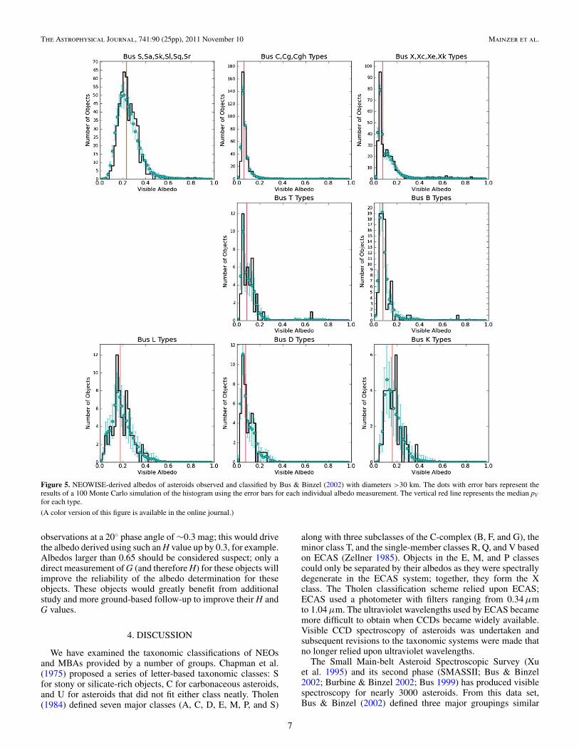
Figure 5. NEOWISE-derived albedos of asteroids observed and classified by Bus & Binzel (2002) with diameters >30 km. The dots with error bars represent theresults of a 100 Monte Carlo simulation of the histogram using the error bars for each individual albedo measurement. The vertical red line represents the median pVfor each type.

(A color version of this figure is available in the online journal.)

observations at a 20◦ phase angle of ∼0.3 mag; this would drivethe albedo derived using such an H value up by 0.3, for example.Albedos larger than 0.65 should be considered suspect; only adirect measurement of G (and therefore H) for these objects willimprove the reliability of the albedo determination for theseobjects. These objects would greatly benefit from additionalstudy and more ground-based follow-up to improve their H andG values.

4. DISCUSSION

We have examined the taxonomic classifications of NEOsand MBAs provided by a number of groups. Chapman et al.(1975) proposed a series of letter-based taxonomic classes: Sfor stony or silicate-rich objects, C for carbonaceous asteroids,and U for asteroids that did not fit either class neatly. Tholen(1984) defined seven major classes (A, C, D, E, M, P, and S)

along with three subclasses of the C-complex (B, F, and G), theminor class T, and the single-member classes R, Q, and V basedon ECAS (Zellner 1985). Objects in the E, M, and P classescould only be separated by their albedos as they were spectrallydegenerate in the ECAS system; together, they form the Xclass. The Tholen classification scheme relied upon ECAS;ECAS used a photometer with filters ranging from 0.34 μmto 1.04 μm. The ultraviolet wavelengths used by ECAS becamemore difficult to obtain when CCDs became widely available.Visible CCD spectroscopy of asteroids was undertaken andsubsequent revisions to the taxonomic systems were made thatno longer relied upon ultraviolet wavelengths.

The Small Main-belt Asteroid Spectroscopic Survey (Xuet al. 1995) and its second phase (SMASSII; Bus & Binzel2002; Burbine & Binzel 2002; Bus 1999) has produced visiblespectroscopy for nearly 3000 asteroids. From this data set,Bus & Binzel (2002) defined three major groupings similar

7

The Astrophysical Journal, 741:90 (25pp), 2011 November 10 Mainzer et al.

Figure 6. NEOWISE-derived albedos of asteroids observed and classified by DeMeo et al. (2009) with diameters >30 km. The dots with error bars represent theresults of a 100 Monte Carlo simulation of the histogram using the error bars for each individual albedo measurement. The vertical red line represents the median pVfor each type.

(A color version of this figure is available in the online journal.)

to Tholen (1984) (the S-, C-, and X-complexes) and splitthem into 26 classes depending on the presence or absenceof particular spectral features or slopes in visible wavelengths.In the system of Bus & Binzel (2002), albedo is not used, andthe short wavelength definition of the taxonomy extends only to0.44 μm. Thus, limitations arise in that, for example, C and Xtypes can be difficult to distinguish without albedo and withoutmeasurements over UV wavelengths. DeMeo et al. (2009) andDeMeo (2010) extended the system of Bus & Binzel (2002) byusing near-infrared spectral features as well as visible, creating asystem of 24 taxonomic types. Neither the Bus & Binzel (2002)nor DeMeo et al. (2009) systems use albedo as a means oftaxonomic classification.

Taxonomic classification systems can provide some under-standing of the compositional nature of asteroids, but they havelimitations. Reflected colors may in some cases reveal mineralabsorption bands that provide diagnostic information on com-

position, but the appearance of these spectral features can beinfluenced by other materials with similar absorption features,material states, particle sizes, illumination angles, etc. Further-more, some bodies’ spectra are generally featureless. For all ofthese reasons, other physical parameters such as albedo becomeimportant for further interpreting composition. We have usedthe classification data compiled in the Planetary Data SystemSmall Body Node by Neese (2010), which aggregates taxo-nomic types for ∼2600 minor planets from various sources.Table 1 gives the average albedos that we have computed fromthe asteroids we have observed with NEOWISE for each of thevarious taxonomic classes in the Tholen, Bus, and Bus–DeMeoschemes. A discussion of the biases that must be consideredwhen comparing the albedos between classes is given below.

In Figure 1, we show the diameter compared to pV for1247 asteroids observed and classified according to the Tholenscheme (Tholen 1989; Xu et al. 1995; Lazzaro et al. 2004),

8

The Astrophysical Journal, 741:90 (25pp), 2011 November 10 Mainzer et al.

Figure 7. NEOWISE-derived ratio pIR/pV for asteroids observed and classified by Tholen (1984). Only asteroids for which pIR/pV could be fitted are included inthis plot. The dots with error bars represent the results of a 100 Monte Carlo simulation of the histogram using the error bars for each individual albedo measurement.The vertical red line represents the median pV for each type.

(A color version of this figure is available in the online journal.)

including 15 NEOs and 1232 MBAs. Figure 2 shows diameterversus pV for the 1524 objects classified according to the Busscheme (Bus & Binzel 2002; Lazzaro et al. 2004), including21 NEOs and 1503 MBAs. Finally, Figure 3 shows the 233asteroids classified according to the DeMeo scheme (14 NEOsand 219 MBAs), which is based heavily on that of Bus. It shouldbe noted that the same objects can have different classificationsaccording to multiple schemes. Since so few NEOs have beenobserved relative to the numbers of MBAs, we have includedthe NEOs in our plots; there are not enough to significantlychange the statistics. In all three schemes, an uptick in theaverage value of pV for smaller diameters (<30 km) can beobserved, regardless of spectral class. There is a notable absenceof small, dark objects, particularly among the C-complex types,yet numerically low albedo objects represent the majority ofthe asteroids in the Main Belt (Masiero et al. 2011). AlthoughDelbo et al. (2003), Harris (2005), and Wolters et al. (2008)

have asserted that there is a real change in albedo with size,these studies are all based upon very small numbers of asteroidsthat are selected from visible light surveys. If there is acorrelation between albedo and size, it is best studied usingthe full NEOWISE data set rather than the relatively smallpopulation that has been selected from visible light surveysfor spectroscopic study to date. When we compare diameterto pV for the entire NEOWISE set selected by the WMOPSpipeline (Mainzer et al. 2011a), we find no strong trend ofincreasing pV with decreasing diameter. The selection bias in thepopulation with taxonomic classifications acts twice. Objectswith higher albedos are more likely to have been discoveredby visible light surveys; a 5 km object with a 40% albedo isnearly a full magnitude brighter than a 5 km object with a20% albedo. Similarly, the 40% albedo object is more likely tohave been selected for the spectroscopic studies necessary fortaxonomic classification because it is more likely to be bright

9

The Astrophysical Journal, 741:90 (25pp), 2011 November 10 Mainzer et al.

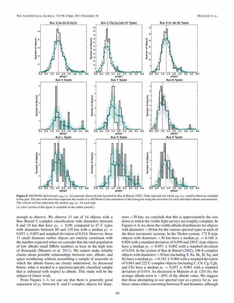
Figure 8. NEOWISE-derived ratio pIR/pV for asteroids observed and classified by Bus & Binzel (2002). Only asteroids for which pIR/pV could be fitted are includedin this plot. The dots with error bars represent the results of a 100 Monte Carlo simulation of the histogram using the error bars for each individual albedo measurement.The vertical red line represents the median pIR/pV for each type.

(A color version of this figure is available in the online journal.)

enough to observe. We observe 11 out of 14 objects with aBus–Binzel C-complex classification with diameters between6 and 10 km that have pV > 0.09, compared to 47 C typeswith diameters between 80 and 110 km with a median pV =0.053 ± 0.002 and standard deviation of 0.014. However, these11 small diameter outlier objects are entirely consistent withthe number expected when we consider that the total populationof low albedo small MBAs numbers at least in the high tensof thousands (Masiero et al. 2011). We cannot make reliableclaims about possible relationships between size, albedo, andspace weathering without assembling a sample of asteroids inwhich the albedo biases are clearly understood. As discussedbelow, what is needed is a spectroscopically classified samplethat is unbiased with respect to albedo. This study will be thesubject of future work.

From Figures 1–3, we can see that there is generally goodseparation of pV between S- and C-complex objects for diam-

eters >30 km; we conclude that this is approximately the sizedown to which the visible light surveys are roughly complete. InFigures 4–6, we show the visible albedo distributions for objectswith diameters >30 km for the various spectral types in each ofthe three taxonomic systems. In the Tholen system, 172 S-typeobjects with diameters >30 km have a median pV = 0.166 ±0.004 with a standard deviation of 0.050 and 250 C-type objectshave a median pV = 0.053 ± 0.002 with a standard deviationof 0.024. In the system of Bus & Binzel (2002), 106 S-complexobjects with diameters >30 km (including S, Sa, Sk, Sl, Sq, andSr) have a median pV = 0.182 ± 0.004 with a standard deviationof 0.043 and 222 C-complex objects (including C, Cb, Cg, Cgh,and Ch) have a median pV = 0.053 ± 0.001 with a standarddeviation of 0.014. As discussed in Mainzer et al. (2011b), theaverage albedo error is ∼20% of the albedo value. We suggestthat those attempting to use spectral type as a proxy for pV usethese values when converting between H and diameter, although

10

The Astrophysical Journal, 741:90 (25pp), 2011 November 10 Mainzer et al.

Figure 9. NEOWISE-derived ratio pIR/pV for asteroids observed and classified by DeMeo et al. (2009). Only asteroids for which pIR/pV could be fitted are includedin this plot. The objects have been separated broadly into S-, C-, X-complexes with S, Sw, D, and L types separated out since they each have more than a handful ofobjects. The dots with error bars represent the results of a 100 Monte Carlo simulation of the histogram using the error bars for each individual albedo measurement.The vertical red line represents the median pIR/pV for each type.

(A color version of this figure is available in the online journal.)

as discussed above, it is unclear whether these values are stillappropriate for objects at sizes smaller than ∼30 km. Figures 2and 3 show that little distinction can be observed between thevarious subtypes in the S- and C-complexes in the Bus andBus–DeMeo schemes at all size ranges. The albedo differencesbetween various spectral types are best preserved in the systemof Tholen (1984). Figures 7–9 give the ratio of the reflectivity inbands W1 and W2 compared with pV for the Bus, Bus–DeMeo,and Tholen schemes, respectively. The mean, standard devia-tion of the mean, standard deviation, and minimum/maximumvalues of pV and pIR/pV for each class (including objects at allsize ranges) are given in Table 1.

S-complex. As expected from Stuart & Binzel (2004) andothers, the S types observed by NEOWISE tend to havesystematically higher albedos than the C types for the Bus,Tholen, and DeMeo classification schemes, although they span

a fairly wide range. The Bus and Bus–DeMeo taxonomicclassification schemes split the S-complex into a number ofdifferent subclasses based on their visible and/or near-infraredslopes and absorption features. Figures 10 and 11 show thebreakdown of pV and pIR/pV , respectively, for the subtypeswith diameters larger than 30 km within the Bus S-complex:S, Sa, Sk, Sl, Sr, and Sq along with the K, L, and A types. Thedistribution of pV is similar for all of these subtypes; any subtledifferences are likely attributable to statistically small numbersof objects for some of the subtypes, with the exception of theK types, which appear to have a somewhat lower albedo asnoted in Tedesco et al. (1989). In the distribution of pIR/pV ,however, we note some slight differences among subclasses,with the S, Sl, and L types showing a slightly higher meanvalue of pIR/pV than the Sq, Sk, and K types. According toBus & Binzel (2002), the S, Sl, and L types have redder slopes

11

The Astrophysical Journal, 741:90 (25pp), 2011 November 10 Mainzer et al.

Figure 10. NEOWISE-derived pV for S-complex asteroids with diameters larger than 30 km classified using the Bus system are separated into S, Sa, Sk, Sl, Sq, andSr classes; we also show the albedos of objects in the K, L, and A classes here. All S-type asteroids have fairly similar albedo distributions. In DeMeo et al. (2009),the Sa, Sk, and Sl classes have been superceded and are no longer used.

(A color version of this figure is available in the online journal.)

than the Sk, Sq, and K types. As with the C, D, and T types,redder VNIR slopes correlate with higher pIR/pV , possiblyindicating that the red slope continues out to 3–4 μm. However,in general, pV and the pIR/pV ratio of most of the Bus S-complexsubtypes are similar. DeMeo et al. (2009) create a new spectralsequence for the S-complex that supercedes the Bus S-complex;in the Bus–DeMeo scheme, the Bus Sa disappears, the Bus Sris converted to the Bus–DeMeo Sa, and the Bus Sl and Skclasses are eliminated. In the future, all of the ∼230 asteroidswith these classifications may be redesignated according to thenewer Bus–DeMeo system. Figures 6 and 9 show the albedoand pIR/pV distributions for objects with diameters larger than30 km and more than a handful of objects per taxonomic class.

It has been asserted that Q-type asteroids are the un-space-weathered cousins of the S-type asteroids, with the Bus–DeMeoSq subtype representing an intermediate state between S and Qtypes (DeMeo et al. 2009). In the Bus–DeMeo system, types

with a w (e.g., Sw, Sqw, Srw) are versions of types with steeperand redder VNIR slopes; DeMeo et al. (2009) attribute thisreddening to the effects of space weathering. Space weatheringis thought to darken and redden surfaces of airless bodiesexposed to radiation; Chapman (2004) and Clark et al. (2002)give overviews of the subject. We have observed 65 MainBelt S types classified according to the Bus–DeMeo systemand 26 MBAs classified as Sw. The S types have a medianpV = 0.224 ± 0.013 with a standard deviation of 0.068, whilethe Sw types have a median pV = 0.239±0.012 with a standarddeviation of 0.095 (see Figure 3). This result suggests that ifspace weathering is at work on the Sw types, it does not maketheir surfaces darken; it is also possible that these objects are notactually weathered or that compositional or surface morphologyvariations such as differences in regolith particle size createsproblems in the comparison between these two groups. Weobserved two NEOs classified as Q type, (2102) and (5143), and

12

The Astrophysical Journal, 741:90 (25pp), 2011 November 10 Mainzer et al.

Figure 11. NEOWISE-derived pIR/pV for S-complex asteroids classified using the Bus system. Classes with steeper, redder VNIR slopes tend to have somewhathigher pIR/pV values.

(A color version of this figure is available in the online journal.)

these objects’ albedos are 0.214 ± 0.095 and 0.227 ± 0.054,respectively. With a sample of only two objects, it is difficultto make a statistically meaningful comparison to the S types,although the albedos are entirely consistent with them. We haveonly three and six Bus–DeMeo Sq and Sqw types, respectively,but their albedos are similar to the S types (see Table 1). Ifthe Sw and Q types that we observed are space weathered, theprocess is not affecting their albedos in the predicted manner.Furthermore, in Masiero et al. (2011), we found that asteroidsin the 5.8 Myr old Karin family have lower albedos than themuch older Koronis family, from which the Karin family isthought to originate (Nesvorny et al. 2002). Determination ofasteroid VNIR spectral slopes used by the Bus and Bus–DeMeosystems can be complicated by instrumental effects as describedin Gaffey et al. (2002) and by reddening of the observed VNIRslopes due to phase effects (Gradie & Veverka 1986). All ofthese results suggest that the picture of space weathering is

complicated, either by compositional variation, variable surfaceproperties, or observational effects.

C-complex. The NEOWISE pV and pIR/pV for the Busand Bus–DeMeo C-complex asteroids are shown for the B,C, Cb, Ch, Cg, and Cgh types in Figures 12 and 13. Inall three taxonomic schemes, the B, C, D, and T types allhave similarly low pV values, ∼0.05. In the VNIR, C-typeasteroids are characterized by relatively flat spectra between0.4 and 1.0 μm with a few, if any, absorption features. In theBus and Bus–DeMeo taxonomic schemes, the C-complex isdifferentiated by the presence or absence of a broad absorptionfeature near 0.7 μm; Bus & Binzel (2002) divided objectswith and without this feature into five further subclasses (C,Cb, Cg, Ch, Cgh) depending additionally on the slope of thespectrum shortward of 0.55 μm. By contrast, the T and D typeshave featureless spectra that are nevertheless characterized bymoderate and steep red VNIR slopes, respectively, whereas the

13

The Astrophysical Journal, 741:90 (25pp), 2011 November 10 Mainzer et al.

Figure 12. NEOWISE-derived pV for C-complex asteroids with diameters larger than 30 km classified using the Bus system are separated into B, C, Cb, Cg, Cgh, andCh classes.

(A color version of this figure is available in the online journal.)

Figure 13. NEOWISE-derived pIR/pV ratio for C-complex asteroids classified using the Bus system are separated into B, C, Cb, Cg, Cgh, and Ch classes. The B-typeasteroids show a somewhat lower pIR/pV ratio than the C-type asteroids, and this is possibly caused by their somewhat blue VNIR slope extending out to 3–4 μm.

(A color version of this figure is available in the online journal.)

14

The Astrophysical Journal, 741:90 (25pp), 2011 November 10 Mainzer et al.

Figure 14. NEOWISE-derived ratio pIR/pV vs. pV for asteroids observed and classified according to the Tholen taxonomic classification scheme. Only asteroids forwhich pIR/pV could be fitted are included in this plot.

(A color version of this figure is available in the online journal.)

Figure 15. NEOWISE-derived ratio pIR/pV vs. pV for asteroids observed and classified according to the system of Bus & Binzel (2002). Only asteroids for whichpIR/pV could be fitted are included in this plot.

(A color version of this figure is available in the online journal.)

15

The Astrophysical Journal, 741:90 (25pp), 2011 November 10 Mainzer et al.

Figure 16. E, M, and P classes that make up the Tholen X type are distinguishable by albedo, as expected from Tholen’s definition.

(A color version of this figure is available in the online journal.)

Figure 17. E, M, and P classes that make up the Tholen X type are not distinguishable by pIR/pV .

(A color version of this figure is available in the online journal.)

B types have a slightly blue slope. The quantity pIR/pV can beextremely useful for differentiating asteroids. While the B, C, D,and T types all have extremely similar pV , their pIR/pV ratios aresignificantly different. As shown in Table 1, the T and D typeshave increasingly larger values of pIR/pV , indicating that thesteep slopes observed between VNIR wavelengths are likely tocontinue through the 3.4 and 4.6 μm WISE bands. A discussionof the possible materials responsible for the spectral appearanceof the primitive Trojan asteroids out to 4 μm can be found inEmery & Brown (2004). Figures 14 and 15 illustrate the utilitythat pIR/pV can provide for distinguishing various taxonomictypes (including the many subclasses within each complex) fromone another in both the Tholen and Bus schemes.

X-complex. The Tholen, Bus, and Bus–DeMeo X types spana wide range of albedos, from ∼0.07 to > 0.6. This wide rangeis to be expected, as the Tholen X type (from which the Bus andBus–DeMeo X types are derived) is comprised of E, M, and Pasteroids which are distinguished on the basis of their albedos(Figure 16; Figure 17 shows the ratio pIR/pV for the Tholen Xtypes). The albedo distribution of the asteroids with Tholen Xclassifications and Bus X types follow a distribution that reflects

the distribution observed in the Main Belt (Masiero et al. 2011).Since neither the Bus nor the Bus–DeMeo taxonomic systemsuse albedo for classification, it is perhaps unsurprising that whentheir X-complex objects are broken down into the X, Xc, Xe,and Xk subclasses (Figure 18 and 19), pV and pIR/pV appear tobe similar for all of them. However, both Bus and Bus–DeMeorecognize the Xe class as being indicative of the high albedo Etypes in the Tholen taxonomy. In Table 2, we assign Tholen-style E, M, and P classifications to X-complex objects that do notalready have E, M, or P classification based on their NEOWISEpreliminary albedos.

Others. The V-type asteroid class was first proposed byTholen (1984); since then, a number of Vestoids have beenidentified both dynamically and spectroscopically as beingrelated to the parent body (4) Vesta. As expected, V-typeasteroids have higher albedos, on average, than the S-complexasteroids. The few asteroids classified as O types by Bus &Binzel (2002) fall within the broad range of the S-complex.

As noted above, we have assumed that pW1 = pW2; futurework will attempt to determine whether or not the albedo at3.4 and 4.6 μm really is the same. To test the degree to which

16

The Astrophysical Journal, 741:90 (25pp), 2011 November 10 Mainzer et al.

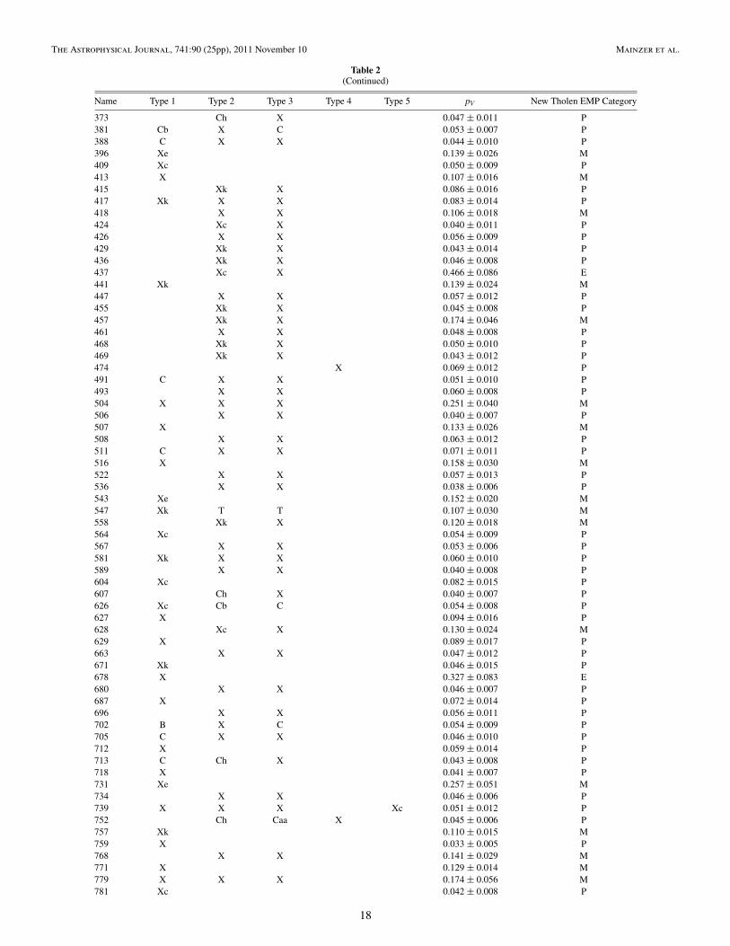
Table 2Asteroids Classified as X Types under Either the Tholen, Bus, or Bus–DeMeo Taxonomic Schemes Can Be Assigned Tholen-style M, E, and

P Classes Based on Their Visible Albedos

Name Type 1 Type 2 Type 3 Type 4 Type 5 pV New Tholen EMP Category

22 X X 0.168 ± 0.038 M46 Xc 0.052 ± 0.011 P56 Xk X X Xk 0.050 ± 0.010 P64 Xe Xe 0.676 ± 0.223 E71 Xe 0.247 ± 0.051 M75 Xk 0.099 ± 0.019 P76 X C 0.049 ± 0.010 P77 Xe Xe 0.153 ± 0.027 M83 X 0.086 ± 0.021 P87 X X X X 0.036 ± 0.008 P97 Xc 0.206 ± 0.046 M99 Xk Xk 0.058 ± 0.010 P107 X X X 0.055 ± 0.013 P110 X Xk 0.170 ± 0.042 M114 Xk K 0.088 ± 0.010 P117 X X X 0.039 ± 0.007 P125 X 0.115 ± 0.022 M129 X 0.157 ± 0.026 M131 Xc CX K 0.164 ± 0.033 M132 Xe Xe 0.119 ± 0.022 M135 Xk 0.153 ± 0.028 M136 Xe 0.164 ± 0.033 M139 X 0.045 ± 0.023 P143 Xc 0.053 ± 0.011 P153 X X 0.047 ± 0.010 P164 X X X 0.043 ± 0.007 P166 Xe Xk X 0.066 ± 0.014 P181 Xk X X Xk 0.079 ± 0.015 P184 X X X 0.106 ± 0.020 M190 X 0.038 ± 0.008 P191 Cb X X Cb 0.043 ± 0.007 P199 X X X D 0.116 ± 0.026 M201 X Xk 0.098 ± 0.021 P209 Xc 0.058 ± 0.010 P214 Xc B B Cg 0.204 ± 0.041 M216 Xe Xe 0.111 ± 0.034 M217 X X 0.043 ± 0.009 P220 Xk X 0.057 ± 0.011 P223 Xc X 0.034 ± 0.006 P224 T X 0.161 ± 0.031 M227 X X 0.060 ± 0.017 P231 X 0.066 ± 0.014 P233 K T T Xk 0.092 ± 0.016 P242 Xc 0.160 ± 0.027 M247 Xc 0.060 ± 0.011 P248 X 0.048 ± 0.019 P250 Xk Xk 0.113 ± 0.022 M255 X X 0.033 ± 0.008 P256 X 0.060 ± 0.011 P259 X X X 0.042 ± 0.009 P260 X X 0.063 ± 0.011 P261 X 0.101 ± 0.015 M268 X X 0.046 ± 0.010 P272 X 0.127 ± 0.018 M273 Xk K 0.118 ± 0.021 M279 X D 0.039 ± 0.006 P304 Xc 0.043 ± 0.007 P307 X X 0.040 ± 0.011 P309 X X 0.058 ± 0.016 P317 Xe 0.505 ± 0.056 E319 X 0.078 ± 0.014 P322 X D 0.074 ± 0.008 P336 Xk 0.046 ± 0.005 P338 Xk 0.163 ± 0.032 M372 B X C 0.065 ± 0.016 P

17

The Astrophysical Journal, 741:90 (25pp), 2011 November 10 Mainzer et al.

Table 2(Continued)

Name Type 1 Type 2 Type 3 Type 4 Type 5 pV New Tholen EMP Category

373 Ch X 0.047 ± 0.011 P381 Cb X C 0.053 ± 0.007 P388 C X X 0.044 ± 0.010 P396 Xe 0.139 ± 0.026 M409 Xc 0.050 ± 0.009 P413 X 0.107 ± 0.016 M415 Xk X 0.086 ± 0.016 P417 Xk X X 0.083 ± 0.014 P418 X X 0.106 ± 0.018 M424 Xc X 0.040 ± 0.011 P426 X X 0.056 ± 0.009 P429 Xk X 0.043 ± 0.014 P436 Xk X 0.046 ± 0.008 P437 Xc X 0.466 ± 0.086 E441 Xk 0.139 ± 0.024 M447 X X 0.057 ± 0.012 P455 Xk X 0.045 ± 0.008 P457 Xk X 0.174 ± 0.046 M461 X X 0.048 ± 0.008 P468 Xk X 0.050 ± 0.010 P469 Xk X 0.043 ± 0.012 P474 X 0.069 ± 0.012 P491 C X X 0.051 ± 0.010 P493 X X 0.060 ± 0.008 P504 X X X 0.251 ± 0.040 M506 X X 0.040 ± 0.007 P507 X 0.133 ± 0.026 M508 X X 0.063 ± 0.012 P511 C X X 0.071 ± 0.011 P516 X 0.158 ± 0.030 M522 X X 0.057 ± 0.013 P536 X X 0.038 ± 0.006 P543 Xe 0.152 ± 0.020 M547 Xk T T 0.107 ± 0.030 M558 Xk X 0.120 ± 0.018 M564 Xc 0.054 ± 0.009 P567 X X 0.053 ± 0.006 P581 Xk X X 0.060 ± 0.010 P589 X X 0.040 ± 0.008 P604 Xc 0.082 ± 0.015 P607 Ch X 0.040 ± 0.007 P626 Xc Cb C 0.054 ± 0.008 P627 X 0.094 ± 0.016 P628 Xc X 0.130 ± 0.024 M629 X 0.089 ± 0.017 P663 X X 0.047 ± 0.012 P671 Xk 0.046 ± 0.015 P678 X 0.327 ± 0.083 E680 X X 0.046 ± 0.007 P687 X 0.072 ± 0.014 P696 X X 0.056 ± 0.011 P702 B X C 0.054 ± 0.009 P705 C X X 0.046 ± 0.010 P712 X 0.059 ± 0.014 P713 C Ch X 0.043 ± 0.008 P718 X 0.041 ± 0.007 P731 Xe 0.257 ± 0.051 M734 X X 0.046 ± 0.006 P739 X X X Xc 0.051 ± 0.012 P752 Ch Caa X 0.045 ± 0.006 P757 Xk 0.110 ± 0.015 M759 X 0.033 ± 0.005 P768 X X 0.141 ± 0.029 M771 X 0.129 ± 0.014 M779 X X X 0.174 ± 0.056 M781 Xc 0.042 ± 0.008 P

18

The Astrophysical Journal, 741:90 (25pp), 2011 November 10 Mainzer et al.

Table 2(Continued)

Name Type 1 Type 2 Type 3 Type 4 Type 5 pV New Tholen EMP Category

789 X Xk 0.139 ± 0.027 M792 X 0.032 ± 0.008 P796 X X X 0.205 ± 0.041 M814 C X X 0.048 ± 0.006 P816 Xc X 0.044 ± 0.008 P834 X X 0.061 ± 0.010 P844 X 0.126 ± 0.022 M850 X X 0.071 ± 0.012 P859 X C 0.060 ± 0.011 P860 X 0.076 ± 0.015 P866 X 0.041 ± 0.008 P872 X 0.111 ± 0.020 M882 X X 0.064 ± 0.009 P892 X X 0.043 ± 0.007 P894 X X 0.115 ± 0.022 M899 X X 0.145 ± 0.026 M907 Xk 0.027 ± 0.007 P917 X X 0.050 ± 0.009 P928 X X 0.038 ± 0.007 P941 X 0.131 ± 0.026 M943 Ch X 0.047 ± 0.007 P949 Xk X 0.051 ± 0.011 P952 X X 0.047 ± 0.004 P965 Xc 0.036 ± 0.006 P972 X X 0.037 ± 0.005 P973 Xk X X 0.066 ± 0.013 P977 X X 0.054 ± 0.009 P983 Xk X 0.028 ± 0.006 P1005 Xk X 0.050 ± 0.010 P1013 Xk X 0.139 ± 0.026 M1014 Xe 0.083 ± 0.017 P1015 Xc 0.046 ± 0.008 P1024 Ch X Caa 0.039 ± 0.012 P1030 X X 0.028 ± 0.004 P1032 X 0.031 ± 0.007 P1039 X 0.056 ± 0.007 P1042 X Caa 0.049 ± 0.010 P1046 Xe 0.110 ± 0.024 M1051 Xc X 0.048 ± 0.006 P1098 Xe 0.174 ± 0.037 M1103 Xk 0.300 ± 0.059 E1104 Xk 0.048 ± 0.008 P1107 Xc 0.054 ± 0.010 P1109 X D 0.039 ± 0.010 P1127 X X 0.032 ± 0.008 P1135 Xk 0.059 ± 0.011 P1146 X X 0.144 ± 0.022 M1149 X X 0.033 ± 0.009 P1154 X X 0.034 ± 0.008 P1155 Xe 0.225 ± 0.053 M1171 X X 0.039 ± 0.007 P1180 Xe X 0.044 ± 0.008 P1181 X 0.091 ± 0.019 P1187 X 0.048 ± 0.009 P1201 Xc 0.033 ± 0.005 P1212 X 0.040 ± 0.007 P1214 Xk 0.055 ± 0.011 P1222 X 0.164 ± 0.042 M1226 Xk D 0.172 ± 0.029 M1244 X X 0.059 ± 0.010 P1251 X 0.638 ± 0.125 E1261 X X 0.056 ± 0.010 P1281 X X 0.060 ± 0.008 P1282 Xe X 0.043 ± 0.008 P1283 X X 0.155 ± 0.027 M1304 X 0.196 ± 0.040 M

19

The Astrophysical Journal, 741:90 (25pp), 2011 November 10 Mainzer et al.

Table 2(Continued)

Name Type 1 Type 2 Type 3 Type 4 Type 5 pV New Tholen EMP Category

1317 Xk X 0.181 ± 0.036 M1318 Xe X 0.173 ± 0.034 M1319 X X 0.096 ± 0.019 P1323 Xc 0.024 ± 0.006 P1327 X 0.050 ± 0.008 P1337 Xk X 0.030 ± 0.009 P1351 Xk Xc X 0.067 ± 0.013 P1352 X 0.145 ± 0.019 M1355 Xe X 0.467 ± 0.114 E1356 X X 0.054 ± 0.011 P1373 Xk 0.152 ± 0.024 M1420 X 0.096 ± 0.018 P1424 X 0.062 ± 0.011 P1428 Xc 0.025 ± 0.008 P1436 X X 0.033 ± 0.005 P1463 X 0.071 ± 0.015 P1469 X X 0.074 ± 0.014 P1490 Xc 0.104 ± 0.024 M1493 Xc 0.069 ± 0.010 P1517 X 0.039 ± 0.006 P1541 Xc 0.097 ± 0.019 P1546 X X 0.115 ± 0.016 M1548 Xk 0.045 ± 0.008 P1571 Xc X 0.128 ± 0.020 M1585 X X 0.029 ± 0.006 P1592 X 0.220 ± 0.039 M1605 X X 0.187 ± 0.034 M1628 X 0.049 ± 0.007 P1638 X 0.117 ± 0.018 M1653 X C 0.668 ± 0.117 E1693 X X 0.047 ± 0.008 P1712 X 0.050 ± 0.010 P1730 Xe 0.189 ± 0.035 M1765 X X 0.136 ± 0.025 M1796 Cb X X 0.044 ± 0.008 P1819 X X 0.058 ± 0.009 P1841 X X 0.057 ± 0.010 P1847 Xc 0.231 ± 0.040 M1860 X 0.100 ± 0.015 P1919 Xe X 0.701 ± 0.034 E1936 Ch X X 0.057 ± 0.004 P1992 Xk X 0.145 ± 0.031 M1995 X 0.063 ± 0.051 P1998 Xc 0.107 ± 0.021 M2001 Xe Xe X 0.841 ± 0.145 E2065 Xc 0.084 ± 0.013 P2073 X 0.154 ± 0.030 M2103 X X 0.139 ± 0.021 M2104 X X 0.104 ± 0.019 M2140 X 0.053 ± 0.007 P2194 Xc 0.183 ± 0.031 M2204 X X X 0.050 ± 0.006 P2303 X X 0.295 ± 0.058 M2306 X 0.132 ± 0.014 M2349 Xc Xk X 0.166 ± 0.031 M2390 X 0.042 ± 0.007 P2407 X X 0.150 ± 0.029 M2444 C X 0.053 ± 0.007 P2489 X Caa 0.059 ± 0.009 P2491 Xe X 0.544 ± 0.102 E2507 Xe 0.133 ± 0.022 M2559 Xk 0.049 ± 0.006 P2560 Xc 0.102 ± 0.014 M2567 Xc 0.156 ± 0.024 M2606 Xk 0.176 ± 0.031 M2634 X X 0.108 ± 0.021 M

20

The Astrophysical Journal, 741:90 (25pp), 2011 November 10 Mainzer et al.

Table 2(Continued)

Name Type 1 Type 2 Type 3 Type 4 Type 5 pV New Tholen EMP Category

2681 Xk 0.228 ± 0.090 M2736 Xc 0.848 ± 0.236 E2861 Xc 0.069 ± 0.011 P2879 X 0.067 ± 0.013 P2996 Xc 0.069 ± 0.012 P3007 X 0.147 ± 0.024 M3109 X 0.064 ± 0.017 P3169 Xe Cb C 0.413 ± 0.095 E3256 X 0.047 ± 0.007 P3262 X 0.138 ± 0.025 M3328 Xc K 0.148 ± 0.030 M3330 X X 0.048 ± 0.008 P3367 X 0.303 ± 0.059 E3381 X 0.517 ± 0.124 E3406 X 0.158 ± 0.025 M3440 X 0.174 ± 0.030 M3445 X X 0.055 ± 0.007 P3451 X 0.049 ± 0.012 P3483 Xk X 0.862 ± 0.088 E3567 Xc 0.087 ± 0.017 P3575 X 0.201 ± 0.039 M3615 X C 0.086 ± 0.016 P3670 X 0.064 ± 0.013 P3686 X 0.064 ± 0.011 P3691 Xc 0.672 ± 0.158 E3704 Xk 0.181 ± 0.035 M3740 X 0.071 ± 0.012 P3762 X 0.513 ± 0.113 E3789 Xk T 0.099 ± 0.016 P3832 X C 0.069 ± 0.016 P3865 Xc 0.238 ± 0.041 M3880 Xe X 0.574 ± 0.130 E3915 Xc C C 0.049 ± 0.005 P3939 X X 0.042 ± 0.009 P3940 T X 0.641 ± 0.108 E3958 Xc 0.574 ± 0.085 E3976 X 0.038 ± 0.010 P3985 X 0.152 ± 0.027 M4006 X 0.070 ± 0.002 P4031 X 0.398 ± 0.092 E4165 XS 0.123 ± 0.025 M4201 X X 0.061 ± 0.013 P4256 Xc 0.210 ± 0.024 M4342 Xc 0.068 ± 0.010 P4353 Xe X 0.138 ± 0.024 M4369 Xk 0.120 ± 0.024 M4424 Xk 0.073 ± 0.014 P4440 X 0.567 ± 0.033 E4460 X X 0.041 ± 0.008 P4461 X 0.135 ± 0.025 M4483 X X 0.215 ± 0.038 M4547 X 0.039 ± 0.007 P4548 Xc 0.206 ± 0.042 M4613 Xe S 0.284 ± 0.036 M4701 Xe 0.053 ± 0.005 P4750 X 0.087 ± 0.010 P4764 X X 0.896 ± 0.118 E4786 Xc 0.534 ± 0.104 E4838 Xc 0.105 ± 0.020 M4839 Xc 0.204 ± 0.039 M4845 X 0.181 ± 0.018 M4942 X 0.631 ± 0.135 E4956 XT 0.167 ± 0.034 M5087 X 0.064 ± 0.007 P5294 X 0.175 ± 0.042 M5301 X C 0.070 ± 0.012 P

21

The Astrophysical Journal, 741:90 (25pp), 2011 November 10 Mainzer et al.

Table 2(Continued)

Name Type 1 Type 2 Type 3 Type 4 Type 5 pV New Tholen EMP Category

5343 X X 0.276 ± 0.042 M5467 X 0.115 ± 0.023 M5588 X 0.163 ± 0.031 M5632 Xc 0.192 ± 0.036 M6051 X X 0.324 ± 0.044 E6057 X X 0.043 ± 0.011 P6249 Xe 0.786 ± 0.147 E6394 Xe X 0.637 ± 0.131 E8795 X C 0.136 ± 0.018 M10261 Xk X 0.079 ± 0.004 P11785 Xc 0.101 ± 0.021 M12281 X 0.040 ± 0.006 P

Notes. We assign the P type to objects with pV < 0.1, E to asteroids with pV > 0.3, and the rest to M type. The various X types are listed fromthe following sources: (1) Bus & Binzel 2002, denoted as Type 1; (2) Lazzaro et al. 2004, denoted as Type 2; (3) Lazzaro et al. 2004, denotedas Type 3; (4) Xu et al. 1995, denoted as Type 4; and (5) DeMeo et al. 2009, denoted as Type 5.

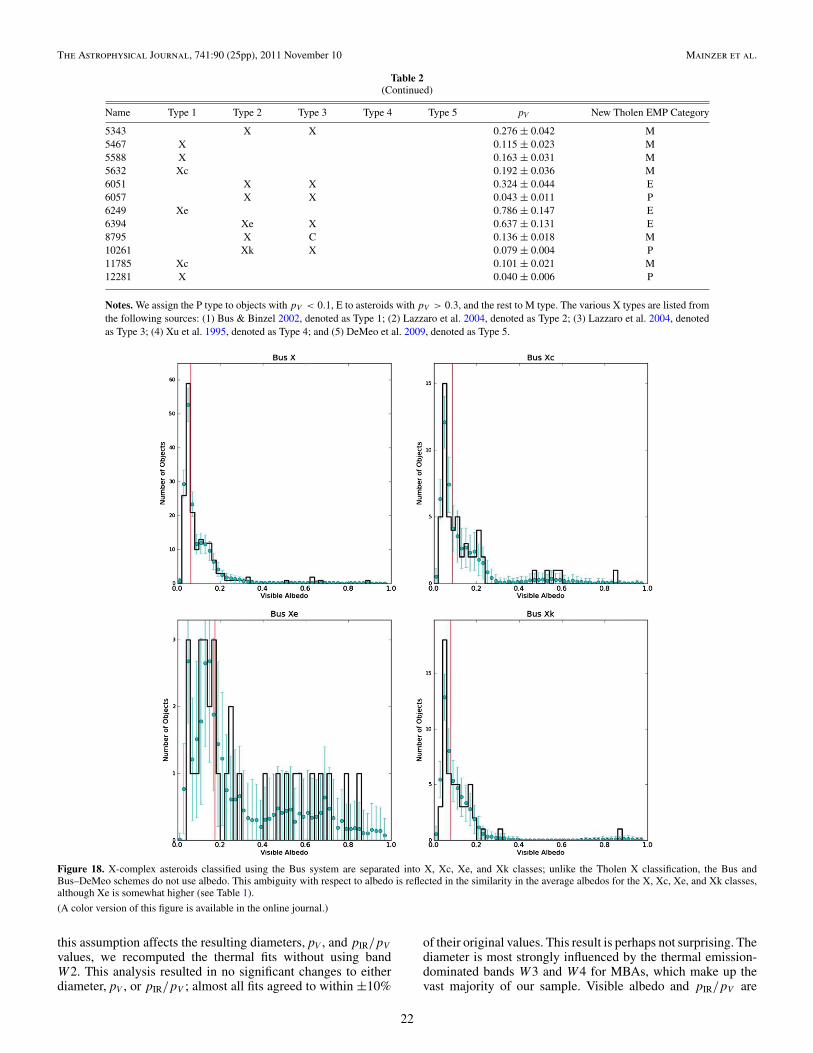
Figure 18. X-complex asteroids classified using the Bus system are separated into X, Xc, Xe, and Xk classes; unlike the Tholen X classification, the Bus andBus–DeMeo schemes do not use albedo. This ambiguity with respect to albedo is reflected in the similarity in the average albedos for the X, Xc, Xe, and Xk classes,although Xe is somewhat higher (see Table 1).

(A color version of this figure is available in the online journal.)

this assumption affects the resulting diameters, pV , and pIR/pV

values, we recomputed the thermal fits without using bandW2. This analysis resulted in no significant changes to eitherdiameter, pV , or pIR/pV ; almost all fits agreed to within ±10%

of their original values. This result is perhaps not surprising. Thediameter is most strongly influenced by the thermal emission-dominated bands W3 and W4 for MBAs, which make up thevast majority of our sample. Visible albedo and pIR/pV are

22

The Astrophysical Journal, 741:90 (25pp), 2011 November 10 Mainzer et al.

Figure 19. X, Xc, Xe, and Xk Bus classes within the X-complex have similar values of pIR/pV .

(A color version of this figure is available in the online journal.)

more heavily influenced by band W1 than W2, since this bandconsists almost entirely of reflected sunlight, while band W2most always has less reflected light than thermal emission.

There are a number of different possible causes of the varia-tions we observe in pIR/pV for different objects. Even a cursoryexamination of mineralogical and meteorite databases yieldsa wealth of different materials with features in wavelengthscovered by bands W1 and W2. Gaffey et al. (2002) and ref-erences therein summarize some of the possible causes of fea-tures in these wavelength regimes: a 3 μm feature indicating thepresence of hydration caused by the fundamental O–H stretchbands of H2O; anhydrous assemblages of mafic silicates con-taining structural OH; possible fluid inclusions; or the presenceof troilite. Rivkin et al. (2000) carried out spectrophotometricobservations of asteroids in the 1.2–3.5 μm region and foundevidence of absorption at 3 μm; they conclude that these areproduced by hydrated minerals. Of the 27 M-type asteroidsstudied in Rivkin et al. (2000), 10 showed evidence of an ab-sorption feature at 3 μm. With NEOWISE, we observed seven ofthese: (22) Kalliope, (77) Frigga, (110) Lydia, (129) Antigone,(135) Hertha, (136) Austria, and (201) Penelope. As Rivkinet al. (2000) report that the depth of the absorption band at 3 μmis only ∼10%–20% of the continuum flux over a fairly narrowrange of wavelengths, we conclude that it would be unlikely toshow a detectable change to pIR/pV given that the W1 band-

pass extends from 2.8 to 3.8 μm (Wright et al. 2010). Theseseven objects have a median pV = 0.157 ± 0.010 and their me-dian pIR/pV = 1.572 ± 0.050. This latter matches the pIR/pV

found for the 33 M-type asteroids shown in Figure 17, whichhave a median pIR/pV of 1.623 ± 0.051 and standard deviationof 0.291. Merenyi et al. (1997) show a number of additionalasteroids with evidence of absorption at 3 μm, including theC-type asteroid (1467) Mashona, which is given as having aband depth of 88%. We find that this asteroid has pIR/pV ∼ 0.9;however, this value is entirely in line with the rest of the C-typeasteroids. It is possible, even likely, that the spread in pIR/pV

that we observe could represent nothing more than the naturalvariation in spectral slope within the various spectral classes.

As discussed above and demonstrated by Figures 1 and 2,caution must be exercised when attempting to generalize thefractional population results presented herein to all NEOs orMBAs. The objects selected for taxonomic classification werechosen on the basis of their discovery by visible light surveys, sothe selection is inherently biased in favor of high albedo objects.Although Stuart & Binzel (2004) compute the relative fractionsof asteroids of various taxonomic types observed throughoutthe solar system, we do not attempt such an undertaking here.C. Thomas et al. (in preparation) compare the albedo distribu-tions of NEOs found using 3.6 and 4.5 μm imaging from theSpitzer Space Telescope to the albedo distributions of MBAs;

23

The Astrophysical Journal, 741:90 (25pp), 2011 November 10 Mainzer et al.

while they find that the NEO albedos are higher than MainBelt albedos for various spectral types, this result is perhapsnot surprising given that the Warm Spitzer sample was drawnfrom optically selected NEOs. We have observed relatively fewNEOs with taxonomic classifications with WISE and will haveto wait until more taxonomic classifications are in hand beforemaking comparisons between NEOs and MBAs. The point ofsuch an exercise would be to determine the relative numbers,compositions, sizes, and distribution of asteroids of various pop-ulations throughout the solar system. We have computed thedebiased size and albedo distributions of the NEOs in Mainzeret al. (2011d) and we are computing similar distributions forthe MBAs, Trojans, and comets. By working with the entireNEOWISE data set, these works can provide a more direct ac-counting for the distribution of asteroid albedos and sizes fordifferent populations.

5. CONCLUSIONS

With the advent of a large, thermal infrared survey of asteroidsthroughout the solar system, the NEOWISE data set offers theopportunity to study the relationship between albedo and variousspectral features with unprecedented clarity. We have computedthe preliminary observed range of possible albedos for thevarious classes using ∼1800 NEOs and MBAs we observedwith NEOWISE. This may allow important physical parametersto be used in the refinement of existing taxonomic classificationschemes or perhaps to allow objects of different types to be morereadily distinguished from one another. Although reasonablygood separation between the two main S and C taxonomiccomplexes can be observed for diameters >30 km, where thevisible light surveys that found them are largely complete, alltaxonomic types and subtypes show an uptick in average albedosat smaller sizes. We attribute this uptick to strong selectionbiases against finding and classifying small, dark objects withVNIR spectroscopy. For objects >30 km, it is clear that amedian albedo can be used based on taxonomic classification.One could assume that the median albedos for smaller sizes aresimilar, but the strong selection biases against small, low albedoobjects in this study preclude us from deriving or verifyingthat these median albedos extend to smaller sizes. Due tothe same selection biases, we are thus unable to comment onthe relationship between size, albedo, and space weathering,although comparison between S and Sw Bus–DeMeo typesshows no evidence that the Sw types are darker at any observedsize scales. The two Q-type objects we observed have nearlyidentical albedos to the S types, but a larger number of classifiedQ types from our data set is needed to confirm this result. Wedo not observe any major distinctions in albedo among the Ssubtypes and C subtypes in the Bus and Bus–DeMeo systems.From an albedo perspective, Figures 1–3 make the Tholensystem stand out as the cleanest. While the Tholen system usesalbedo to separate the X types into E, M, and P classes, albedois not used to define the remainder of the classes in the Tholensystem.

There is a strong selection bias in the taxonomic classifica-tion schemes and average albedos presented here (clearly inFigures 1–3) and by other observers. First, since all the objectsselected for taxonomic classification have been drawn from vis-ible light surveys, the relative fractional abundance of objectswith particular taxonomic types is biased toward higher fractionsof high albedo objects. Second, within a particular taxonomicclass, lower albedo objects are less likely to have been observedbecause they tend to be fainter in visible light: this will skew

the average albedo for a particular taxonomic type higher. Be-cause of these biases, when the average albedo is used to convertfrom absolute H magnitude to size, artificially smaller sizes forasteroids will be found. This speaks to the need to assemble asample of objects with taxonomic classifications that are drawnfrom the NEOWISE thermal infrared survey to mitigate biasesagainst low albedo objects.

With the four infrared wavelengths given by the WISE dataset, we are able to derive the ratio of the albedo at 3.4 and 4.6 μmto the visible albedo. We have shown that taxonomic types withsteeply red spectral slopes in VNIR wavelengths tend to havehigher pIR/pV values. We hypothesize that this is caused bythe fact that the spectral slopes continue to rise from visiblethrough the near-infrared to the W1 and W2 wavelengths forthese objects. For example, we have shown that spectral types Tand D can be distinguished from the C types by examining theirpIR/pV , even though they have virtually identical pV . Subclasseswithin the S- and C-complexes generally have similar visiblealbedos and largely similar pIR/pV ratios. However, pIR/pV canonly be computed when a sufficiently high fraction of reflectedsunlight is present in either bands W1 or W2. The bias againstlow albedo objects is present in the determination of pIR, in thatdark objects are less likely to have enough reflected sunlight inbands W1 or W2 to allow pIR to be computed. As before, wecaution against generalizing the average pIR/pV values we havegiven here to entire populations or classes of objects in light ofthe presence of these biases.

This work shows that the NEOWISE data set offers a newmeans of exploring the connections between taxonomic classi-fications derived from VNIR spectroscopy and spectrophotom-etry. Future work will explore the relationship between visiblealbedo and the 3–4 μm albedo to VNIR spectroscopic proper-ties in greater detail. The value of the NEOWISE data set willonly be enhanced by the acquisition of additional VNIR ancil-lary data. More data would be beneficial for two reasons. First,we require a measurement of H in order to determine pV andpIR/pV , so more accurate H and G values will result in moreaccurate albedos. Second, by obtaining taxonomic classificationof low albedo objects drawn from the NEOWISE sample, wecan reduce the bias within each taxonomic class against loweralbedo objects. With the NEOWISE data set, we now have ac-cess to a means of directly computing debiased size and albedodistributions that are not as subject to the biases against lowalbedo objects as objects selected for classification and study byvisible light surveys.

This publication makes use of data products from the Wide-field Infrared Survey Explorer, which is a joint project of theUniversity of California, Los Angeles, and the Jet PropulsionLaboratory/California Institute of Technology, funded by theNational Aeronautics and Space Administration. This publica-tion also makes use of data products from NEOWISE, whichis a project of the Jet Propulsion Laboratory/California In-stitute of Technology, funded by the Planetary Science Divi-sion of the National Aeronautics and Space Administration. Wegratefully acknowledge the extraordinary services specific toNEOWISE contributed by the International AstronomicalUnion’s MPC, operated by the Harvard-Smithsonian Center forAstrophysics, and the Central Bureau for Astronomical Tele-grams, operated by Harvard University. We thank the paper’sreferee, Prof. Richard Binzel, for his helpful contributions. Wealso thank the worldwide community of dedicated amateur andprofessional astronomers devoted to minor planet follow-up

24

The Astrophysical Journal, 741:90 (25pp), 2011 November 10 Mainzer et al.

observations. This research has made use of the NASA/IPAC Infrared Science Archive, which is operated by theJet Propulsion Laboratory, California Institute of Technol-ogy, under contract with the National Aeronautics and SpaceAdministration.

REFERENCES

Binzel, R., Rivkin, A., Stuart, J., et al. 2004, Icarus, 170, 259Bowell, E., Hapke, B., Domingue, D., et al. 1989, in Asteroids II, ed. R. P.

Binzel, T. Gehrels, & M. S. Matthews (Tuscon, AZ: Univ. Arizona Press),524

Burbine, T., & Binzel, R. 2002, Icarus, 159, 468Bus, S. 1999, PhD thesis, MITBus, S., & Binzel, R. 2002, Icarus, 158, 146Chapman, C. 2004, Annu. Rev. Earth Planet. Sci., 32, 539Chapman, C., Morrison, D., & Zellner, B. 1975, Icarus, 25, 104Clark, B., Hapke, B., Pieters, C., & Britt, D. 2002, in Asteroids III, ed. W. F.

Bottke, A. Cellino, P. Paolicchi, & R. P. Binzel (Tuscon, AZ: Univ. ArizonaPress), 585

Cutri, R. M., Wright, E. L., Conrow, T., et al. 2011, Explanatory Supplementto the WISE Preliminary Data Release Products, http://wise2.ipac.caltech.edu/docs/release/prelim/expsup/

Delbo, M., Harris, A. W., Binzel, R. P., Pravec, P., & Davies, J. K. 2003, Icarus,166, 116

DeMeo, F. 2010, PhD thesis, La Variation Compositionnelle Des Petits CorpsTravers le Sytme Solaire, Observatoire de Paris

DeMeo, F., Binzel, R., Slivan, S., & Bus, S. 2009, Icarus, 202, 160Emery, J. P., & Brown, R. H. 2004, Icarus, 170, 131Gaffey, M. 2010, Icarus, 209, 564Gaffey, M., Burbine, T., & Binzel, R. 1993, Meteoritics, 28, 161Gaffey, M., Cloutis, E. A., Kelley, M. S., & Reed, K. L. 2002, in Asteroids III,

ed. W. F. Bottke, A. Cellino, P. Paolicchi, & R. P. Binzel (Tuscon, AZ: Univ.Arizona Press), 183

Gradie, J., & Veverka, J. 1986, Icarus, 66, 455Grav, T., Mainzer, A. K., Bauer, J., et al. 2011, ApJ, in pressHarris, A. W. 1998, Icarus, 131, 291Harris, A. W. 2005, in IAU Symp. 229, Asteroids, Comets, Meteors, ed. D.

Lazzaro, S. Ferraz-Mello, & J. A. Fernandez (Cambridge: Cambridge Univ.Press), 449

Harris, A. W., Mueller, M., Lisse, C., & Cheng, A. 2009, Icarus, 199, 86Harris, A. W., & Young, J. W. 1988, BAAS, 31, 06Harris, A. W., Young, J. W., Contreiras, L., et al. 1989, Icarus, 81, 365Kaasalainen, M., Pravec, P., Krugly, Y., et al. 2004, Icarus, 167, 178Lazzaro, D., Angeli, C., Carvano, J., et al. 2004, Icarus, 172, 179Lebofsky, L., & Spencer, J. 1989, Asteroids II (Tucson, AZ: Univ. Arizona

Press), 128Lebofsky, L., Veeder, G., Lebofsky, M., & Matson, D. 1978, Icarus, 35, 336Liu, F., Cutri, R., Greanias, G., et al. 2008, Proc. SPIE, 7017, 16Mainzer, A., Bauer, J., Grav, T., et al. 2011a, ApJ, 731, 53Mainzer, A., Eisenhardt, P., Wright, E. L., et al. 2005, Proc. SPIE, 5899, 262Mainzer, A., Grav, T., Bauer, J., et al. 2011d, ApJ, in pressMainzer, A., Grav, T., Masiero, J., et al. 2011b, ApJ, 736, 100Mainzer, A., Grav, T., Masiero, J., et al. 2011c, ApJ, 737, L9Masiero, J., Mainzer, A., Grav, T., et al. 2011, ApJ, 741, 68Matson, D. (ed.) 1986, The IRAS Asteroid and Comet Survey, JPL D-3698

(Pasadena, CA: JPL)Merenyi, E., Howell, E. S., Rivkin, A. S., & Lebofsky, L. A. 1997, Icarus, 129,

421Neese, C. (ed.) 2010,Asteroid Taxonomy V6.0, EAR-A-5-DDR-TAXONOMY-

V6.0, NASA Planetary Data SystemNesvorny, D., Bottke, W. F., Dones, L., & Levison, H. F. 2002, Nature, 417,

720Pravec, P., Scheirich, P., Kusnirak, P., et al. 2006, Icarus, 181, 63Rivkin, A., Howell, E., Lebofsky, L., Clark, B., & Britt, D. 2000, Icarus, 145,

351Stuart, J., & Binzel, R. 2004, Icarus, 170, 295Tedesco, E., Noah, P., Noah, M., & Price, S. 2002, AJ, 123, 1056Tedesco, E., Williams, J. G., Matson, D. L., et al. 1989, AJ, 97, 580Tholen, D. 1984, PhD thesis, Univ. ArizonaTholen, D. 1989, in Asteroids II, ed. R. P. Binzel, T. Gehrels, & M. S. Matthews

(Tucson, AZ: Univ. Arizona Press), 298Tholen, D. J. (ed.) 2009,Asteroid Absolute Magnitudes V12.0, EAR-A-5-DDR-

ASTERMAG-V12.0, NASA Planetary Data SystemThomas, C., & Binzel, R. 2010, Icarus, 205, 419Veeder, G., Hanner, M. S., Matson, D. L., et al. 1989, AJ, 97, 1211Warner, B., Harris, A., & Pravec, P. 2009a, Icarus, 202, 134Wolters, S., Green, S. F., McBride, N., & Davies, J. K. 2008, Icarus, 193, 535Wright, E. L., et al. 2010, AJ, 140, 1868Xu, S., Binzel, R., Burbine, T., & Bus, S. 1995, Icarus, 115, 1Zellner, B., Tholen, D., & Tedesco, E. 1985, Icarus, 61, 355

25