CSLS Conference on the State of Living Standards and the Quality of Life in Canada

October 30 - 31, 1998 Château Laurier Hotel, Ottawa, Ontario

Centre for theStudy of Living Standards

Centre d'étude desniveaux de vie

Neighbourhoods, Social Capital and the Long-term Prospects forChildren

Miles CorakStatistics Canada

Andrew Heisz Statistics Canada

Session 4 Sustainability II: Intergenerational Bequests and the Well-being of ChildrenOctober 30 2:15 PM - 4:15 PM

NEIGHBOURHOODS, SOCIAL CAPITAL, AND THELONG-TERM PROSPECTS OF CHILDREN

Miles Corak and Andrew Heisz

Statistics Canada24F R.H. Coats Building,Ottawa Ontario K1A 0T6

Voice: (613) 951-9047 FAX: (613) 951-5403Internet: coramil@statcan.ca

PAPER PREPARED FOR THE CSLS CONFERENCE ON THESTATE OF LIVING STANDARDS AND THE QUALITY OF LIFE IN CANADA

October 1998

Neighbourhoods, Social Capital, and theLong-Term Prospects of Children

Any discussion of the quality of life in a society must take into account the well-being of

its children; not only their well-being as citizens like any other group of citizens, but also

their future well-being—that is, their preparedness for adulthood. In fact, the reason

“child poverty” has such a resonance among policy makers, and indeed among Canadians

in general, has in part to do with the potential long-term consequences of experiencing

low-income during childhood. Does being raised by low-income parents scar individuals

so that they go on to become low-income adults in their turn? Conversely, do the children

of the well-to-do rise to the top of the income distribution as adults? Is the underlying

process determining outcomes of these sorts fair? An issue that evokes these kinds of

questions touches upon what we must in some sense mean by the “quality of life.”

The process determining the capacity of children to become successful and self-

sufficient adults is complicated and involves not just parental income, but also the

broader functioning of the family, as well as the roles of community and state.

Communities and neighbourhoods play a variety of roles in preparing children for adult

life. These span both economic and social factors; a neighbourhood is where individuals

live, but it is also the connections and relationships they have to the others around them.

Our objective in this paper is to examine the relationship between the long-term labour

market prospects of children—their earnings and market incomes as adults—and the

characteristics of the neighbourhood in which they lived, focusing on what we refer to as

2

economic conditions and social capital in the neighbourhood. The analysis begins with a

short review of what is known about the relationship between family income and the

adult incomes of children in Canada. However, the specific question motivating our

research is: what role does “neighbourhood”—both the geographic and the social space—

play in determining the adult labour market success of children?

This question has received a great deal of attention among social scientists in the

United States in part because of the long-lasting concern in that country with the plight of

inner-city neighbourhoods and the development of a so-called “underclass.” In particular,

neighbourhood influences have received increasing emphasis as a result of the work of

William Julius Wilson (1987, 1996) who detailed the degradation of inner-city areas of

Chicago associated with structural changes in employment, the migration of middle-class

residents, as well as the resulting decline in community infrastructure and norms of

behaviour. As a result there has been a plethora of research including most recently that

by: Aaronson (1996), Akerlof (1997), Brooks-Gunn et al. (1993) (1997a,b), Case and

Katz (1991), Corcoran et al.(1992), Evans et al.(1992), Gaviria and Raphael (1997),

Solon et al. (1997). It is difficult to offer a definitive summary of this literature, but the

general picture to emerge would seem to suggest that neighbourhood influences do not

represent a major influence on child attainments when data representative of the entire

country are used. The empirical research is not nearly as developed in Canada in spite of

the fact that public policy debates increasingly use the term “social capital,” a phrase that

refers, like “neighbourhood,” to the role of community in determining the prospects of

children.

3

We address this gap in knowledge by grouping Canadian neighbourhoods along

economic and social dimensions, and examining the adult labour market outcomes of

teenagers according to the economic conditions and social capital of the area in which

they grew up. We find that their ultimate adult incomes and earnings is only loosely tied

to the income of their parents. In the large, the Canadian labour market is characterized

by a good deal of equality of opportunity. But this overall result is misleading as we also

find that the influence of parental income is strongly conditioned by the characteristics of

the neighbourhood in which the children are raised. Neighbourhood economic conditions

and social capital—as we define these terms—are particularly important in understanding

the income disparities between the members of the next generation of young adults. Adult

labour market outcomes differ between teenagers raised in different neighbourhoods in a

way that has little to do with the differences in average parental income. In particular, our

results suggest that: [1] economic conditions in the neighbourhood, as reflected mainly in

the neighbourhood unemployment rate and youth unemployment rate, have a strong

association with adult incomes and earnings of teenagers; [2] the social capital of the

neighbourhood, as reflected in the educational attainment of the adults and the affluence

of the neighbourhood, also displays such a relationship, though perhaps not as strong; and

[3] social capital at the individual level, as measured in the strength of the child’s ties to

the neighbourhood, also has a noteworthy association with earnings and income in

adulthood. These factors—neighbourhood economic conditions and social capital, as well

as the capacity of children to access them—are so strong that differences in parental

income play a distinctly secondary role in determining the pattern of relative advantages

in the next generation. There are certain caveats associated with this interpretation of our

4

findings, but if these can be shown in future work to be minor, then the results suggeset

that if government policy is concerned about the long-term prospects of children it needs

to address more than simply the level of family income, and recognize the importance of

the local macroeconomic and social climate in which children are raised.

1. Methods

Our starting point is the growing literature on intergenerational income and earnings

mobility, surveyed in for example Björklund and Jäntti (1998), Mulligan (1997, chapter

7), and Solon (1997). The major analytical approach in this literature is based on the

estimation of a simple linear model linking a child’s income (as an adult) to his or her

parents’ income. If y reprsents the natural logarithm of permanent income, t the child’s

generation, and t-1 the parents’ generation then the standard approach is to use least

squares to estimate:

yi(t) = �0 + �1 yi(t-1) + 0i (1)

where the data are at the individual level with i representing a parent-child pair, and 0i is

a random component usually assumed to be distributed as N��� 12). The constant term

(�0) represents the change in income common to generation t, while the coefficient �1

indicates the extent to which income is associated with that of the parents’, that is the

extent of intergenerational mobility.1 If �1 is less than one the income distribution is said

to regress to the mean: while parents with incomes above (or below) the mean will have

1 This coefficient is often called the intergenerational income elasticity, and is related to the correlationbetween parent and child incomes by the standard deviation of the logarithm of incomes:

�1 ! 1>y(t)@ � 1>y(t-1)]ZKHUH 1> @ VLJQLILHV WKH VWDQGDUG GHYLDWLRQ� 6LQFH WKH VWDQGDUG GHYLDWLRQ RI WKH ORJDULWKP RI LQFRPHV LV DQ

index of inequality, �1 ZLOO HTXDO ! LI WKH GHJUHH RI LQFRPH LQHTXDOLW\ LV WKH VDPH EHWZHHQ WKH JHQHUDWLRQV�

5

children with above (or below) average income levels the deviation from the mean will

not be as great. (If it is greater than one the deviation from the mean will be even greater

in the next generation.) The larger �1 (even if it is less than one) the more likely that an

individual as an adult will occupy the same economic position as his or her parents, that

is the greater the persistence in intergenerational incomes. Even small values of �1 can be

associated with substantial advantages for the children of the well-off. For example, the

income advantage associated with having a high-income father relative to having a low-

income father is (YH / YL) �1, where the upper case Y denotes the level of income. In

Canada, the ratio of the average income of men (working full-year full-time) in the top

quintile to those in the bottom quintile during 1981 was 3.84. This would imply an

income advantage in the next generation of 14% if �1 were 0.1. This is a substantial

difference, but it becomes even more so with higher values: 31% if �1 were 0.2 and over

70% if it were as high as 0.4.2

It is easy to understand, therefore, why an accurate estimate of �1 has been the

main concern of studies that adopt this approach. However, the implicit assumption often

made is that both �0 and �1 are the same for all children regardless of their place in the

income distribution. There are both strong theoretical reasons and, at least for Canada,

strong empirical results to suggest that this assumption may not be valid.3 In particular, if

2 The emerging consensus seems to be that 0.4 (or even higher) is not a bad estimate of theintergenerational earnings elasticity in the United States and the United Kingdom, while 0.2 or perhapseven less seems appropriate for Canada and some European countries. See Corak and Heisz (1998) andFortin and Lefebvre (1998) for Canadian evidence.

3 For example, Mulligan (1997) offers a clear exposition of various models of intergenerational mobilityand points out the possibility of non-linearities. In particular, �1 will be higher for those parents who areborrowing-constrained and cannot make the optimal level of investment in the education of their children.Durlauf (1996) offers a model of non-linearities based upon neighbourhood differences. Corak and Heisz(1998a) illustrate that the value of �1 varies across the income distribution in Canada in a way that can beinterpreted by the borrowing-constraints model.

6

neighbourhoods differ in social capital and if social capital is an important influence on

the long-term prospects of children—over and above the fact that average family income

varies between neighbourhoods—then this would be reflected in different values of �0

and �1. Neighbourhood differences in �1 reflect differences in how family income is

transformed into the economic status of the next generation; differences in �0 reflect

differences in the factors common to all members of the neighbourhood. If this is the case

then the income advantage of someone from a high status neighbourhood relative to

someone from a low status neighbourhood would be:

The relative incomes of the children in adulthood is the result of three factors as reflected

in the three terms of this equation: differences in �0 between the neighbourhoods in

which they were raised, differences in the incomes of their parents, and differences in the

�1 between their neighbourhoods. The first and third terms offer a means of assessing the

relative importance of neighbourhood characterisitcs, beyond the fact that average

incomes vary.

Equations (1) and (2) form the analytical framework for our research. Using

equation (1) we estimate values for �0 and �1 by neighbourhood, and then use equation

(2) to assess the relative advantage of individuals living in a reference neighbourhood

relative to all others. The analysis is based upon income tax information on a cohort of

young men and women in 1995 and upon similar information on their parents during the

late 1970s and early 1980s. Briefly, we select a sample of individuals aged 16 to 19 years

(2) 11

1 11

1

0

0

Lt

��

Lt

Ht

�

�

�

YY

Y

e

eYY

LH

H

L

H

L

t

H

t

�

u

�

�

u

¸¹

ᬩ

§�

¸̧¹

·¨̈©

§

7

of age in 1982, who filed an income tax return in that year (while still living with their

parents) and who are therefore 29 to 32 years of age in 1995. We relate the adult earnings

and market income (defined as the total of earnings, self-employment income, asset

income and other market incomes) of the chidren to that of their parents between 1978

and 1982. 4 The sample size is very large, numbering up to almost 850,000 parent-child

pairs, and not subject to problems of attrition or reporting errors that are endemic to

survey data. We attach census geographic codes to this information by using the postal

code reported on the parents’ 1982 T1 form.5 This permits us to link neighbourhood

characteristics from the 1981 census to the individual parent-child pair.

2. The Definition of Neighbourhoods

The first challenge in implementing the framework described in equation (2) concerns

how to define a neighbourhood in terms of “social capital.” While this is an often used

term, it is not clearly defined nor easily measured. Becker (1996, p.4) simply states that

social capital “incorporates the influence of past actions by peers and others in an

individual’s social network and control system.” Portes (1998) offers a broad review of

the concept, noting in particular the difficulty of extending it from an individual asset to a

feature of communities and nations. One of the clearest definitions probably belongs to

Coleman (1988, 1990) who considers social captial to have three dimensions: the set of

expectations and obligations (essentially reputations) that develop in a community, the set

4 The construction of the data is described in the Appendix to Corak and Heisz (1998b). The data used hereis an updated version of that employed in Corak and Heisz (1998b) in that it uses 1995 incomes of thechildren, and includes individuals who were raised in lone-mother households. For a discussion of dataquality and the potential for sample selection bias see Corak and Heisz (1988a).

5 The way in which this is accomplished is described in an appendix available from the authors.

8

of information channels, and the set of norms or sanctions that exist at the community

level. While all three are important in the intergenerational mobility of children, he

focuses on the conditions that allow the latter to arise. A well-established set of norms or

sanctions can serve to reinforce parental human capital investment in children. In

particular, he suggests that this will be strongest when the relationship between children,

say in the context of a school, is mirrored at the level of the parents so that the parents’

friends are also the parents of their children’s friends. He refers to this as

“intergenerational closure.” In this sense, social capital might be considered as an aspect

of network or peer group effects, as in Becker’s interpretation.

While Coleman does not offer a direct measure of intergenerational closure he

suggests that an apporpriate proxy is the number of times the child has moved, in

particular the number of school changes, as this indicates a lack of continuity and hence

the breaking up of networks. Parents who have moved into a new neighbourhood are

likely, in Coleman’s argument to not have as much information or be as well connected

as those who are long-term residents. Nonetheless, social capital as defined is not

tangible and inherently difficult to measure with the kind of data sets generally available

to analysts. 6 Accordingly our approach is rather eclectic. We use information from the

1981 Canadian Census at the Census Tract (CT) and Provincial Census Tract (PCT)

level. These categories are defined by Statistics Canada to correspond to what roughly

might be considered a neighbourhood, and they certainly capture important aspects of

geographic but probably also of social space. Even so it should be recognized that CTs

6 Since social capital is also related the amount of time invested in children by parents Coleman suggeststhat the number of siblings, the presence of a working mother, or being raised in a lone-parent family arerelevant measures: more siblings, a two-earner family, or a single parent family leading to inferior childoutcomes.

9

and PCTs may not reflect the neighbourhood as experienced by residents, who may relate

to smaller areas within it or to areas outside of it (Furstenberg Jr. and Huges 1997, p.34).

This being said the advantage of using the 1981 census is that all areas of Canada are

tracted, either as CTs or as PCTs. The Provincial Census Tract program has since been

discontinued so that only larger urban areas are tracted in other censuses. All 24 Census

Metropolitan Areas (CMAs) and 12 of the 88 Census Agglomerations (CAs) are census

tracted in the 1981 Census, while the remaining 76 CAs and all rural areas are

provincially census tracted. Thus the availability of PCTs allows us to distinguish

neighbourhoods in smaller urban areas (the CAs), and also to include rural areas in the

analysis. There are 4,967 geographic units used in our analysis with an average

population of 4,833, varying from 262 to a maximum of 20,483.7

Our approach is to: first, define a host of characteristics for each CT/PCT that

may relate to the characteristics of the neighbourhood important in determining child

attainments; second, to use factor analysis to group these characteristics into a small

number of factors and score each CT/PCT along these fewer dimensions; third, to cluster

7 A Census Tract refers to a permanent small geostatistical area established in large urban communitieswith the help of local specialists interested in urban and social science research. Census Tracts are reviewedand approved by Statistics Canada according to the following criteria: (1) the boundaries must followpermanent and easily recognized lines on the ground; (2) the population must be between 2,500 and 8,000with a preferred average of 4,000 persons, except for Census Tracts in the central business district, majorindustrial zones, or in periperal rural or urban areas that may have either a lower or a higher population; (3)the area must be as homogeneous as possible in terms of economic status and social living conditions; (4)the shape must be as compact as possible. Provincial Census Tracts exist in the area not included in theCensus Tract programme. The populations captured in PCTs vary between 3,000 to 8,000, with a preferredsize of 5,000. As much as possible boundaries of PCTs follow permanent physical features and /orgeographic units suggested by the provinces.

Overall there are 5,088 Census Tracts and Provincial Census Tracts. We excluded 117 of thesebecause the population of 15 to 19 year olds was less than 50, and a further four because they had missingvalues for at least one of the characteristics used in the analysis (in all cases this was the average value ofdwellings). The reason for the first exclusion was the need to ensure that derived characteristics werereasonably accurate, especially those pertaining to the cohort of main interst. These exclusions have aminimal effect on our estimate of the total Canadian population leading to an underestimate of only about78,500 from the total of 24,084,000. Of the 4,967 geographic units used in our analysis 3,185 are censustracts, and 1,782 provincial census tracts.

10

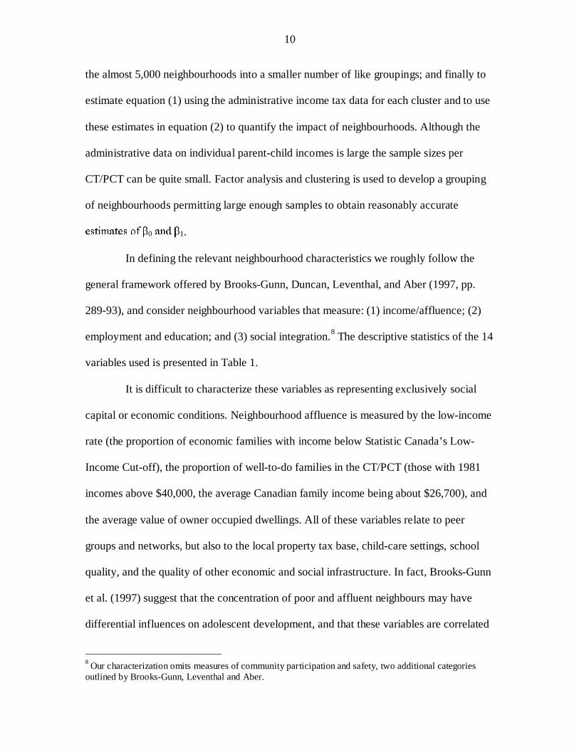
the almost 5,000 neighbourhoods into a smaller number of like groupings; and finally to

estimate equation (1) using the administrative income tax data for each cluster and to use

these estimates in equation (2) to quantify the impact of neighbourhoods. Although the

administrative data on individual parent-child incomes is large the sample sizes per

CT/PCT can be quite small. Factor analysis and clustering is used to develop a grouping

of neighbourhoods permitting large enough samples to obtain reasonably accurate

HVWLPDWHV RI �0 DQG �1.

In defining the relevant neighbourhood characteristics we roughly follow the

general framework offered by Brooks-Gunn, Duncan, Leventhal, and Aber (1997, pp.

289-93), and consider neighbourhood variables that measure: (1) income/affluence; (2)

employment and education; and (3) social integration.8 The descriptive statistics of the 14

variables used is presented in Table 1.

It is difficult to characterize these variables as representing exclusively social

capital or economic conditions. Neighbourhood affluence is measured by the low-income

rate (the proportion of economic families with income below Statistic Canada’s Low-

Income Cut-off), the proportion of well-to-do families in the CT/PCT (those with 1981

incomes above $40,000, the average Canadian family income being about $26,700), and

the average value of owner occupied dwellings. All of these variables relate to peer

groups and networks, but also to the local property tax base, child-care settings, school

quality, and the quality of other economic and social infrastructure. In fact, Brooks-Gunn

et al. (1997) suggest that the concentration of poor and affluent neighbours may have

differential influences on adolescent development, and that these variables are correlated

8 Our characterization omits measures of community participation and safety, two additional categoriesoutlined by Brooks-Gunn, Leventhal and Aber.

11

with other measures of socio-economic status. In a similar way the six variables under the

rubric of employment and education relate to the economic conditions in the

neighbourhood, but also more broadly to human and social capital. Three unemployment

rates are used to, one the one hand, capture the economic opportunities in the

neighbourhood, but also peer group effects. It is for this reason that the youth

unemployment rate and the proprotion of youth receiving unemployment insurance are

defined for the population 20 to 24 years old, the cohort slightly older than the group of

adolescents at the heart of the analysis. The three remaining variables may offer proxies

for the role models or peer groups influencing educational decisions of youths: the

proportion of the adult population with univeristy education, the proportion with less than

high school education, and the proportion of youths not attending school. All of these

variables are also associated with the economic status of the neighbourhood. Finally,

social integration refers to a group of variables that attempt to measure the ethnic and

religious aspects of the community (the proportion of immigrants and the proportion

belonging to the two most homogenous religious groups that could be readily identified

in the Census). These might be taken to offer an indication of the extent of closure in

Coleman’s terms, but they could certainly also be associated with economic conditions.

In addition, Borjas (1992, 1993) points out the importance of “ethnic capital” in referring

to the impact of the environment in which immigrant families pass their skills and

attitudes along to their children. He argues that the labour market skills of the next

generation depends not just on investments made by parents, but also on the average

quality of skills in the ethnic community.9 This “ethnic capital” seems to be another

9 His analysis of data from the U.S. suggests that “the intergenerational progress of workers belonging toethnic groups that have relatively low levels of human capital is retarded by the low average quality of the

12

dimension of social capital. The proportion of immigrants in the population may be a

rough indicator of degree of the strength of these community ties, and the proportion of

the population speaking a non-official language may indicate the skill level or at least

signal the challenges the community may have in relating to the wider society and

political system. Finally, adapting Coleman’s emphasis on residental moves, the

proportion of the population that did not reside in the same CT/PCT during the last

Census (five years earlier) may reflect the degree to which networks are underdeveloped

in the community. That being said it may also reflect economic conditions, newer or

more affluent neighbourhoods attracting families able to move up, and less affluent

neighbourhoods attracting those experiencing declines in their economic well-being.

The use of factor anlysis reveals that these 14 dimensions can be reduced to

three separate factors. We refer to these as social capital, economic conditions, and ethnic

capital. The factor loadings underlying this characterization are presented in Table 2. We

call that term determined for the most part by the education variables, the proportion of

affluent, and the dwelling value as Social Capital, and the term driven by the overall

unemployment rate and the youth unemployment rate as Economic Conditions. The third

term is associated pretty well exclusively with the proportion of immigrants and the

proportion speaking a language other than French or English, and therefore referred to as

Ethnic Capital. These factor loadings are scored and used to develop three indices, each

centered around a mean of zero and with a standard deviation of one; higher values of

each index indicating either more social capital, better economic conditions, and more

ethnic capital.

group.” (Borjas 1992, p.124)

13

These indices are used to partition the 4,967 CT/PCTs into 100 clusters. A broad

picture of the nature of these clusters is presented in Table 3. On average there are 50

CT/PCTs per cluster, but this varies from a minimum of one (10 cases) to a maximum of

454. Clusters have on average a total population of 240,050, and an average 15 to 19 year

old population of 22,986.

3. Results

Following Corak and Heisz (1998a), we undertake two sets of analyses: one based on the

relationship between parent-child earnings, another on parent-child market incomes. As

mentioned earlier, market income is a concept broader than earnings, incorporating self-

employment income, asset income (interest, divididends, and rental income), and other

incomes with market sources. These are all defined as reported on the T1 form that

Canadians are required to submit to the tax authorities. Market income is probably a

better measure of the total purchasing power available to the household. It should be

noted that we explicitly exclude all non-market sources of income, that is government

transfers. We do this because our focus is on the ability of the next generation to succeed

in the marketplace. However, the distinction between market income and earnings may

be important in understanding the role of self-employment and the direct transfer of

financial resources in the intergenerational process.10

10 As such our analysis does not address issues asssociated with the intergenerational transmission of thereliance on government support. This issue, however, might be considered to fall into the scope of ourstudy in two ways: as a direct indication of the self-reliance of adult children, but also as an assessment ofthe long-term implications government transfer payments. A complete analysis is precluded by the fact thatIncome Assistance payments generally are not reported to Revenue Canada, this is particularly so duringthe period in which we capture parental incomes.

14

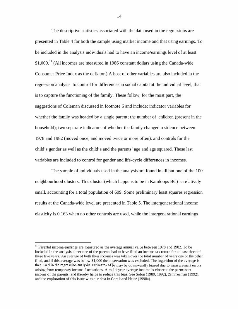
The descriptive statistics associated with the data used in the regressions are

presented in Table 4 for both the sample using market income and that using earnings. To

be included in the analysis individuals had to have an income/earnings level of at least

$1,000.11 (All incomes are measured in 1986 constant dollars using the Canada-wide

Consumer Price Index as the deflator.) A host of other variables are also included in the

regression analysis to control for differences in social capital at the individual level, that

is to capture the functioning of the family. These follow, for the most part, the

suggestions of Coleman discussed in footnote 6 and include: indicator variables for

whether the family was headed by a single parent; the number of children (present in the

household); two separate indicators of whether the family changed residence between

1978 and 1982 (moved once, and moved twice or more often); and controls for the

child’s gender as well as the child’s and the parents’ age and age squared. These last

variables are included to control for gender and life-cycle differences in incomes.

The sample of individuals used in the analysis are found in all but one of the 100

neighbourhood clusters. This cluster (which happens to be in Kamloops BC) is relatively

small, accounting for a total population of 609. Some preliminary least squares regression

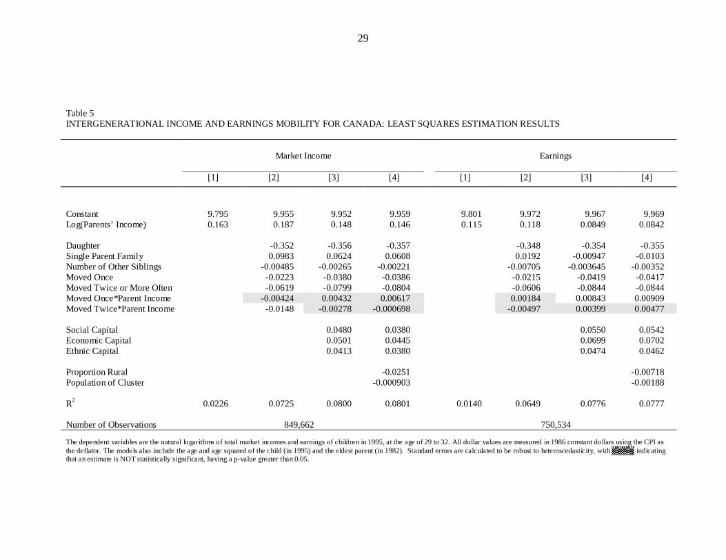
results at the Canada-wide level are presented in Table 5. The intergenerational income

elasticity is 0.163 when no other controls are used, while the intergenerational earnings

11 Parental income/earnings are measured as the average annual value between 1978 and 1982. To beincluded in the analysis either one of the parents had to have filed an income tax return for at least three ofthese five years. An average of both their incomes was taken over the total number of years one or the otherfiled, and if this average was below $1,000 the observation was excluded. The logarithm of the average isWKHQ XVHG LQ WKH UHJUHVVLRQ DQVO\VLV� (VWLPDWHV RI �1 may be downwardly biased due to measurement errorsarising from temporary income fluctuations. A multi-year average income is closer to the permanentincome of the parents, and thereby helps to reduce this bias. See Solon (1989, 1992), Zimmerman (1992),and the exploration of this issue with our data in Corak and Heisz (1998a).

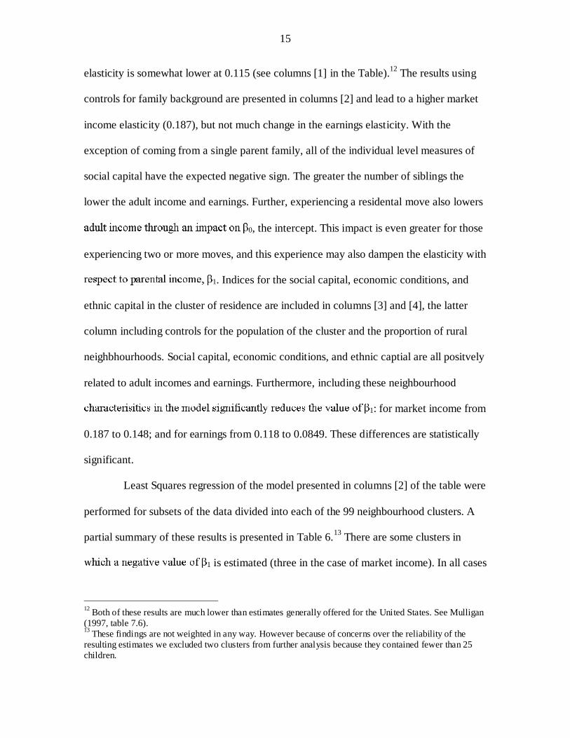
15

elasticity is somewhat lower at 0.115 (see columns [1] in the Table).12 The results using

controls for family background are presented in columns [2] and lead to a higher market

income elasticity (0.187), but not much change in the earnings elasticity. With the

exception of coming from a single parent family, all of the individual level measures of

social capital have the expected negative sign. The greater the number of siblings the

lower the adult income and earnings. Further, experiencing a residental move also lowers

DGXOW LQFRPH WKURXJK DQ LPSDFW RQ �0, the intercept. This impact is even greater for those

experiencing two or more moves, and this experience may also dampen the elasticity with

UHVSHFW WR SDUHQWDO LQFRPH� �1. Indices for the social capital, economic conditions, and

ethnic capital in the cluster of residence are included in columns [3] and [4], the latter

column including controls for the population of the cluster and the proportion of rural

neighbhourhoods. Social capital, economic conditions, and ethnic captial are all positvely

related to adult incomes and earnings. Furthermore, including these neighbourhood

FKDUDFWHULVLWLFV LQ WKH PRGHO VLJQLILFDQWO\ UHGXFHV WKH YDOXH RI �1: for market income from

0.187 to 0.148; and for earnings from 0.118 to 0.0849. These differences are statistically

significant.

Least Squares regression of the model presented in columns [2] of the table were

performed for subsets of the data divided into each of the 99 neighbourhood clusters. A

partial summary of these results is presented in Table 6.13 There are some clusters in

ZKLFK D QHJDWLYH YDOXH RI �1 is estimated (three in the case of market income). In all cases

12 Both of these results are much lower than estimates generally offered for the United States. See Mulligan(1997, table 7.6).13 These findings are not weighted in any way. However because of concerns over the reliability of theresulting estimates we excluded two clusters from further analysis because they contained fewer than 25children.

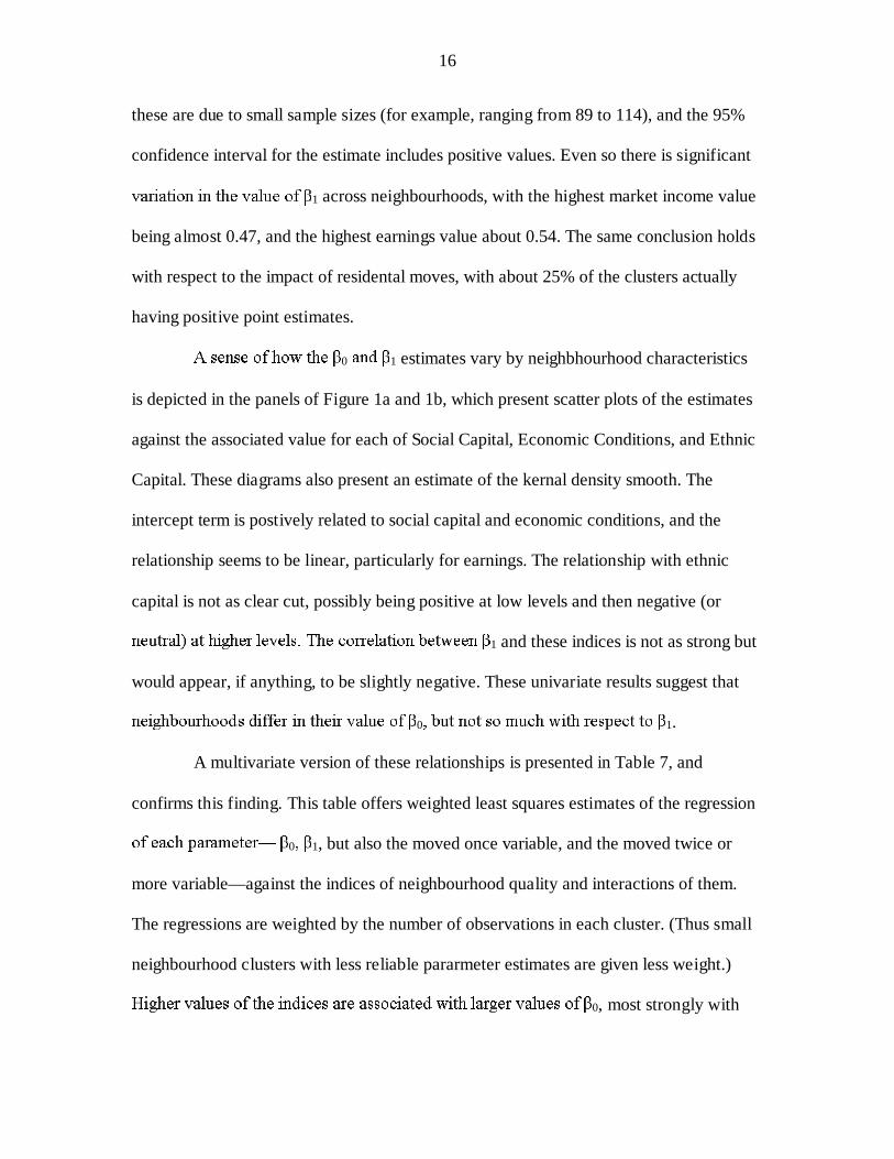
16

these are due to small sample sizes (for example, ranging from 89 to 114), and the 95%

confidence interval for the estimate includes positive values. Even so there is significant

YDULDWLRQ LQ WKH YDOXH RI �1 across neighbourhoods, with the highest market income value

being almost 0.47, and the highest earnings value about 0.54. The same conclusion holds

with respect to the impact of residental moves, with about 25% of the clusters actually

having positive point estimates.

$ VHQVH RI KRZ WKH �0 DQG �1 estimates vary by neighbhourhood characteristics

is depicted in the panels of Figure 1a and 1b, which present scatter plots of the estimates

against the associated value for each of Social Capital, Economic Conditions, and Ethnic

Capital. These diagrams also present an estimate of the kernal density smooth. The

intercept term is postively related to social capital and economic conditions, and the

relationship seems to be linear, particularly for earnings. The relationship with ethnic

capital is not as clear cut, possibly being positive at low levels and then negative (or

QHXWUDO� DW KLJKHU OHYHOV� 7KH FRUUHODWLRQ EHWZHHQ �1 and these indices is not as strong but

would appear, if anything, to be slightly negative. These univariate results suggest that

QHLJKERXUKRRGV GLIIHU LQ WKHLU YDOXH RI �0� EXW QRW VR PXFK ZLWK UHVSHFW WR �1.

A multivariate version of these relationships is presented in Table 7, and

confirms this finding. This table offers weighted least squares estimates of the regression

RI HDFK SDUDPHWHU² �0� �1, but also the moved once variable, and the moved twice or

more variable—against the indices of neighbourhood quality and interactions of them.

The regressions are weighted by the number of observations in each cluster. (Thus small

neighbourhood clusters with less reliable pararmeter estimates are given less weight.)

+LJKHU YDOXHV RI WKH LQGLFHV DUH DVVRFLDWHG ZLWK ODUJHU YDOXHV RI �0, most strongly with

17

economic conditions and least with ethnic capital. (All of these relationships seem to be

slightly stronger with respect to the earnings model.) The proportion of the total variance

H[SODLQHG E\ WKHVH YDULDEOHV LV DERXW �� WR ���� LPSO\LQJ WKDW YDULDWLRQ LQ WKH �0’s is

closely related to neighbourhood conditions. The partitioning of the CT/PCTs by the

Social Capital, Economic Conditions and Ethnic Capital indices is being reflected in the

intercept term. Futher, the intergenerational elasticities seem to be negatively associated

with the neighbourhood indicators. Higher Social Capital, better Economic Conditions,

and higher Ethnic Capital seem to reduce the association between parent child incomes.

The adult outcomes of individuals coming from lower quality neighbourhoods has a

tighter association to their parents’ income/earnings than for those from high quality

QHLJKERXUKRRGV� (YHQ VR WKH YDULDWLRQ RI WKH �1’s is less clsoely to tied to neighbourhood

FKDUDFWHULVWLFV WKDQ WKH YDULDWLRQ LQ WKH �0’s, with less than 50% of the total variance

being explained in the case of market incomes and less than 40% in the case of earnings.

Finally, higher social capital seems to attenuate, but not completely eliminate, the

negative impact of moving on child incomes. The other variables do not seem to play a

role, and with one exception none of the indices are statistically significant for the

coefficient associated with the individual moving twice or more. These models fit even

less well than the others suggesting that much of the variation in the moves parameter has

little to do with neighbourhood quality. Moving has an impact on the long-term prospects

of children that is not linked to the quality of the neighbourhood being moved into.

The impact of these results is more clearly illustrated by using them in equation

(2). We predict the income advantage of someone living in the cluster with the greatest

population relative to each of the other 96 clusters by using the relevant parameter

18

estimates and setting the income levels to the average incomes in the cluster. We then

repeat the calculation three times: once letting only the intercept terms differ between the

clusters, once letting only average incomes vary, and finally letting only the

intergenerational elasticities vary. In other words, each of the three terms in equation (2)

take their predicted value, while the others are set to one. The results are depicted in

Figure 2 for market income, and Figure 3 for earnings. In both figures the clusters are

ordered by the magnitude of the total effect. Individuals in about 7 clusters obtain less

than 80% of the income of those residing in the modal cluster, and those in about 10 are

in same situation with respect to earnings. In fact, the individuals from a few

neighbourhoods have less than 60% of the income/earnings of the reference case.

Each of the three other lines in the Figures can be interpreted as what the total

relative advantage of those in the modal cluster would be if the other two factors played

no role. (The product of these three lines equals the total impact.) The first implication is

WKDW GLIIHUHQFHV LQ �1 between neighbourhoods make little difference to the income

advantage of living in any particular neighbourhood. Rather, differences in

QHLJKERXUKRRG LQFRPHV DQG GLIIHUHQFHV LQ �0 are the major correlates of the differences

in child outcomes across neighbourhoods. In the case of earnings the impact of

differences in intercepts tracks the total impact very closely with the possible exception

of the very bottom and top extremes. Even in these clusters, however, it remains the

dominant influence. The disparity in average income between the worse off

neighbourhoods and the modal neighbourhood would lead to an earnings difference of

only about 10% in the next generation. The fact that children from these neighbourhoods

end up earning 20 to 45% less than their counterparts has much more to do with a broader

19

set of forces than simply the earnings of their parents. A similar conclusion holds for the

earnings advantage of those at the top end of the earnings distribution.

,Q WKH FDVH RI PDUNHW LQFRPH LW ZRXOG DSSHDU WKDW GLIIHUHQFHV LQ �0 are more

important in determining the relative disadvantage of those not doing as well as the

modal cluster, while income disparities are as important or more important in

determining the relative advantage of those doing better, especially those at the very top.

A relative market income advantage of 30 to over 50%—as predicted for the top three

neighbourhoods— has a great deal to do with the second term of equation (2).14 This

differs from the results for earnings. In an accounting sense relative neighbourhood

incomes are more important in characterizing the circumstances of those from well-to-do

neighbourhoods because market income can be so much larger than earnings. For

example, the parents in the top neighbourhood cluster have an average market income of

over $118,000, and the ratio used in the second term of equation (2) is 3.73. In contrast,

the parents in the top earnings cluster have an average earnings of about $68,000, and the

equivalent earnings ratio is 2.61. However, the more substantive implication has to do

with the fact that those with substantial market incomes have more avenues to affect an

intergenerational transfer to their children. The successful self-employed can transfer an

“entrepreneurial” capital to their offspring (Dunn and Holtz-Eakin, 1996). This may

include a set of attitudes that encourage self-employment, a set of contacts or networks

14,Q IDFW� WR VXJJHVW WKDW GLIIHUHQFHV LQ �1 do not matter may be a simplification. The formulation of

HTXDWLRQ ��� LV VXFK WKDW WKH VHFRQG WHUP LPSOLHV WKDW �1 changes with each comparison being made. Thisdoes not seem to make a difference in the analysis of earnings, but it does for some market income clusters.%RWK GLIIHUHQFHV LQ LQFRPH DQG GLIIHUHQFHV LQ �1 are driving the sharp rise in the impact of relative incomesdepicted in Figure 1 for the top four or five neighbourhoods. However, reconfiguring equation (2) so thatWKH �1 in the second term remains constant at the value for the reference neighbourhood leads to a patternthat does not change the substantive conclusion described in the text. (However, the income advantage ofthe most advantaged individuals is, at slightly over 30%, not as great.)

20

that reduce the difficulties to self-employment, as well as financial resources that ease

financial barriers to pursuing self-employment. In a similar vein, those with significant

incomes and assets are in a position to have made an optimal amount of investment in the

education of their children. As suggested by Becker and Tomes (1986) this would imply

that further investments are made as direct financial transfers so that the children end up

having significant levels of assets and derive an income from them. All of these

DUJXPHQWV LPSO\ WKDW WKH UHODWLYH UROH RI QHLJKERXUKRRGV²DV UHIOHFWHG LQ �0—is

diminished.

)LJXUHV � DQG � GHSLFW WKH LPSDFW RQ �0 of our other individual level measure of

social capital, experiencing a move. The relative income advantage/disadvantage due to

GLIIHUHQFHV LQ �0 from Figures 2 and 3 are juxtaposed with an estimate of the first term in

equation (2) for individuals experiencing two or more moves. (The results, not shown, for

those experiencing one move are the same, but not as great in magnitude.) The reference

case throughout is an individual from the modal cluster who did not experience a move as

a child. The major conclusion to be drawn from these figures, which is foreshadowed in

Table 7, is that residential moves are associated with inferior child outcomes regardless

of the quality of the neighbourhood. Someone raised in the modal cluster who

experienced two or more moves as a young teen earns about 10% less than his or her

counterpart who did not experience a move. This relative disadvantage is roughly the

same throughout the distribution of neighbourhoods (the exception being the very top and

very bottom clusters). In general, children who have moved are at a disadvantage as

adults regardless of to which neighbourhood they moved.

21

4. Conclusions and Caveats

22

BIBLIOGRAPHY

AARONSON, Daneil (1996). “Using Sibling Data to Estimate the Impact ofNeighbourhoods on Children’s Educational Outcomes.” Federal Reserve Board ofChicago, unpublished.

AKERLOF, George A. (1997). “Social Distance and Social Decisions.” Econometrica.Vol. 65, No.5, pp. 1005-27.

BECKER, Gary S. (1996). Accounting for Tastes. Cambridge Massachusetts: HarvardUniversity Press.

__________ and Nigel Tomes (1986). “Human Capital and the Rise and Fall ofFamilies.” Journal of Labor Economics. Vol. 4, No.3 part 2, pp. S1-S39.

BJÖRKLUND, A. and M. Jäntti (1998). “Intergenerational Mobility of Economic Status:Is the United States Different?” Stockholm University, Swedish Institute for SocialResearch Working Paper.

BORJAS, George J. (1993). “The Intergenerational Mobility of Immigrants.” Journal ofLabor Economics. Vol.11, No.1, pp.113-35.

__________ (1992). “Ethnic Capital and Intergenerational Mobility.” Quarterly Journalof Economics. Vol. 107, No.1, 123-50.

BROOKS-GUNN, Jeanne, Greg J. Duncan, and J. Lawerence Aber (1997a) (editors).Neighbourhood Poverty. Volume I Context and Consequences for Children. NewYork: Russell Sage Foundation.

BROOKS-GUNN, Jeanne, Greg J. Duncan, and J. Lawerence Aber (1997b) (editors).Neighbourhood Poverty. Volume II Policy Implications in StudyingNeighbourhoods. New York: Russell Sage Foundation.

BROOKS-GUNN, Jeanne, Greg J. Duncan, Tama Leventhal and J. Lawerence Aber(1997). “Lessons Learned and Future Directions for Research on theNeighborhoods in Which Children Live.” In BROOKS-GUNN, Jeanne, Greg J.Duncan, and J. Lawerence Aber (editors). Neighbourhood Poverty. Volume IIPolicy Implications in Studying Neighbourhoods. New York: Russell SageFoundation.

23

BROOKS-GUNN, Jeanne, Greg J. Duncan, Pamela Kato Klebanov, and Naomi Sealand(1993). “Do Neighbourhoods Influence Child and Adolescent Development?”American Journal of Sociology. Vol. 99, No.2, pp. 353-95.

CASE, A.C. AND Lawerence J. Katz (1991). “ The Company You Keep: The Effects ofFamily and Neighbourhood on Disadvantaged Youth.” NBER Working Paper No.3705.

COLEMAN, James S. (1990). Foundations of Social Theory. Cambridge Massachusetts:Harvard University Press.

__________ (1988). “Social Capital in the Creation of Human Capital.” AmericanJournal of Sociology. Vol. 94 Supplement, pp. S95-S120.

CORAK, Miles and Andrew Heisz (1998a). “The Intergenerational Earnings and IncomeMobility of Canadian Men: Evidence from Longitudinal Income Tax Data.”Journal of Human Resources. Forthcoming.

__________ (1998b). “How to Get Ahead in Life: Some Correlates of IntergenerationalIncome Mobility in Canada.” In Miles Corak (editor). Labour Markets, SocialInstitutions, and the Future of Canada’s Children. Ottawa: Statistics Canada,Catalogue No. 89-553-xpb.

CORCORAN, Mary, Roger Gordon, Deborah Laren, and Gary Solon (1992). “TheAssociation Between Men’s Economic Status and Their Family and CommunityOrigins.” Journal of Human Resources. Vol. 27, No. 4, 575-601.

DURLAUF, Steven N. (1996). “A Theory of Persistent Income Inequality.” Journal ofEconomic Growth. Vol. 1, No.1, pp. 75-94.

EVANS, William N., Wallace E. Oates, and Robert M. Schwab (1992). “Measuring PeerGroup Effects: A Study of Teenage Behavior.” Journal of Political Economy. Vol.100, No. 5, pp. 966-91.

FORTIN, Nicole M. and Sophie Lefebvre (1998). “Intergenerational Income Mobility inCanada.” In Miles Corak (editor). Labour Markets, Social Institutions, and theFuture of Canada’s Children. Ottawa: Statistics Canada, Catalogue No. 89-553-xpb.

GAVIRIA, Alejandro and Steven Raphael (1997). “School-based Peer Effects andJuvenile Behavior.” University of California, San Diego. Discussion Paper 97-21.

MULLIGAN, Casy B. (1997). Parental Priorties and Economic Inequality. Chicago:University of Chicago Press.

24

PORTES, Alejandro (1998). “Social Capital: Its Origins and Applications in ModernSociology.” Annual Review of Sociology. Vol. 24, pp. 1-24.

SOLON, Gary, Marianne E. Page, and Greg J. Duncan (1997). “Correlations betweenNeighboring Children in Their Subsequent Educational Attainment.” Unpublished.

SOLON, Gary (1997). “Intergenerational Mobility in the Labor Market.” Fothcoming inDavid Card and Orley Ashenfelter (editors). Handbook of Labor Economics.Amsterdam: North Holland.

__________ (1992). “Intergenerational Income Mobility in the United States.” AmericanEconomic Review. Vol. 82, No.3, pp. 393-408.

__________ (1989). “Biases in the Estimation of Intergenerational EarningsCorrelations.” Review of Economics and Statistics. Vol. 71, No.1, pp. 172-74.

WILSON, William Julius (1996). When Work Disappears: The World of the New UrbanPoor. New York: Alfred A. Knopf.

__________ (1987). The Truly Disadvantaged: The Inner City, the Underclass, andPublic Policy. Chicago: University of Chicago Press.

ZIMMERMAN, David J. (1992). “Regression Toward Mediocirty in Economic Stature.”American Economic Review. Vol. 82, No.3, pp. 409-29.

25

Table 1CHARACTERISTICS OF CENSUS TRACTS AND PROVINCIAL CENSUS TRACTS

Average Minimum Maximum

1. INCOME / AFFLUENCEProportion of Economic Families below the LICO 0.138 0 0.703Proportion of Census Families with Income above $40,000 0.163 0 0.866Average Value of Dwellings $72,747 0 $545,030

2. EMPLOYMENT AND EDUCATIONUnemployment Rate 7.9 0 43.6Unemployment Rate of 20 to 24 year olds 12.2 0 100Proportion of 20 to 24 year olds receving UI 0.156 0 0.753Proportion of Population 25+ with a University Education 0.169 0 0.757Proportion of Population 25+ with Less Than Grade 9 Education 0.257 0 0.710Proportion of 15 to 19 year olds not attending school 0.316 0 0.924

3. SOCIAL INTEGRATIONProportion of Population who are Immigrants 0.160 0 0.713Proportion of Population who speak a non-official language 0.131 0 0.872Proportion of Population who are Catholic 0.481 0 1.0Proportion of Population who are Jewish 0.12 0 0.905Proportion of Population 5+ who moved since last Census 0.531 0 0.846

Note: Total Sample size is 4,967 Census Tracts and Provincial Tracts from the 1981 Census, consisting of 3,185 Census Tracts and1,782 Provincial Census Tracts. The total population varies from 262 to 20,483 with an average of 4,833. All dollar values arebased on 1981 information.

26

Table 2RESULTS FROM THE FACTOR ANALYSIS OF NEIGHBOURHOOD CHARACTERISTICS

Social Economic EthnicCaptial Conditions Capital

1. INCOME / AFFLUENCEProportion of Economic Families below the LICO -0.558 0.408 0.256Proportion of Census Families with Income above $40,000 0.876 -0.204 0.110Average Value of Dwellings 0.640 -0.277 0.396

2. EMPLOYMENT AND EDUCATIONUnemployment Rate -0.263 0.857 -0.138Unemployment Rate of 20 to 24 year olds -0.043 0.815 -0.167Proportion of 20 to 24 year olds receving UI -0.325 0.484 -0.385Proportion of Population 25+ with a University Education 0.801 -0.196 0.198Proportion of Population 25+ with Less Than Grade 9 Education -0.694 0.567 0.103Proportion of 15 to 19 year olds not attending school -0.587 0.003 0.039

3. SOCIAL INTEGRATIONProportion of Population who are Immigrants 0.158 -0.353 0.803Proportion of Population who speak a non-official language -0.123 -0.2690.813Proportion of Population who are Catholic -0.229 0.530 -0.145Proportion of Population who are Jewish 0.315 0.036 0.302Proportion of Population 5+ who moved since last Census -0.012 0.380 -0.174

Variance Explained by each Factor 3.329 2.904 1.933

Note: Table entries are Factor Loadings from….

27

Table 3DESCRIPTIVE CHARACTERISTICS OF NEIGHBHOURHOOD CLUSTERS

Average StandardDeviation

Minimum Maximum

Total Population per Cluster 240,050 458,331 609 2,239,280Total 15 to 19 year old Populaton per Cluster 22,987 44,245 58 217,101Number of CT/PCTs per Cluster 49.7 89.2 1 454

Social Capital 0.410 1.759 -2.557 5.283Economic Conditions 0.582 1.315 -2.690 5.365Ethnic Capital 0.956 1.394 -1.724 4.492

Table 4DESCRIPTIVE STATISTICS OF PARENT CHILD DATA USED IN THE REGRESSION ANALYSIS

Market Income Earnings

Average Median StandardDeviation

Minimum Maximum Average Median StandardDeviation

Minimum Maximum

Number of observations = 849,662 Number of observations =750,534

Child’s 1995 Income 22,606 20,764 66,757 1,000 58,297,015 22,458 21,178 17,329 1,000 3,692,884Averge Parental Income1 41,323 36,897 39,829 1,000 8,105,157 36,019 34,253 24,659 1,000 1,945,390

Log(Child’s Income) 9.756 9.941 0.810 6.908 17.881 9.773 9.961 0.793 6.908 15.122Log(Parents’ Income) 10.394 10.516 0.746 6.908 15.908 10.245 10.441 0.819 6.908 14.481

Daughter 0.431 0 1 0.436 0 1Single Parent Family 0.120 0 1 0.115 0 1Number of Children2 2.560 1 19 2.546 1 19Moved Once 0.161 0 1 0.164 0 1Moved Twice or More Often 0.055 0 1 0.056 0 1Moved Once*Parent Income 1.670 0 14.5 1.681 0 14.2Moved Twice*Parent Income 0.561 0 15.3 0.568 0 14.5Child’s Age 30.6 1.1 29 32 30.6 1.1 29 32Child’s Age Squared 936 67 841 1,024 935 67 941 1,024Parents’ Age3 48.2 6.6 28 72 47.9 6.5 28 72Parents’ Age Squared 2,363 653 784 5,184 2,343 642 784 5,184

Social Capital 0.064 -0.124 0.902 -2.864 5.284 0.075 -0.110 0.896 -2.864 5.284Economic Capital -0.076 -0.242 0.868 -2.734 5.603 -0.077 -0.239 0.865 -2.734 5.603Ethnic Capital -0.086 -0.313 0.901 -1.778 4.784 -0.078 -1.778 0.905 -0.302 4.784

Observations per Cluster 8,582 1,604 16,587 14 79,932 7,581 1,469 14,507 13 70,004

Notes: (1) Income from both parents averaged over 1978 to 1982. (2) Number of Children present in the Household . ( 3) Age of the eldest parent.The moved variables are defined as any residental move between 1978 and 1982.

29

Table 5INTERGENERATIONAL INCOME AND EARNINGS MOBILITY FOR CANADA: LEAST SQUARES ESTIMATION RESULTS

Market Income Earnings

[1] [2] [3] [4] [1] [2] [3] [4]

Constant 9.795 9.955 9.952 9.959 9.801 9.972 9.967 9.969Log(Parents’ Income) 0.163 0.187 0.148 0.146 0.115 0.118 0.0849 0.0842

Daughter -0.352 -0.356 -0.357 -0.348 -0.354 -0.355Single Parent Family 0.0983 0.0624 0.0608 0.0192 -0.00947 -0.0103Number of Other Siblings -0.00485 -0.00265 -0.00221 -0.00705 -0.003645 -0.00352Moved Once -0.0223 -0.0380 -0.0386 -0.0215 -0.0419 -0.0417Moved Twice or More Often -0.0619 -0.0799 -0.0804 -0.0606 -0.0844 -0.0844Moved Once*Parent Income -0.00424 0.00432 0.00617 0.00184 0.00843 0.00909Moved Twice*Parent Income -0.0148 -0.00278 -0.000698 -0.00497 0.00399 0.00477

Social Capital 0.0480 0.0380 0.0550 0.0542Economic Capital 0.0501 0.0445 0.0699 0.0702Ethnic Capital 0.0413 0.0380 0.0474 0.0462

Proportion Rural -0.0251 -0.00718Population of Cluster -0.000903 -0.00188

R2 0.0226 0.0725 0.0800 0.0801 0.0140 0.0649 0.0776 0.0777

Number of Observations 849,662 750,534

The dependent variables are the natural logarithms of total market incomes and earnings of children in 1995, at the age of 29 to 32. All dollar values are measured in 1986 constant dollars using the CPI asthe deflator. The models also include the age and age squared of the child (in 1995) and the eldest parent (in 1982). Standard errors are calculated to be robust to heteroscedasticity, with shading indicatingthat an estimate is NOT statistically significant, having a p-value greater than 0.05.

30

Table 6SUMMARY OF ESTIMATED PARAMETERS FROM LEAST SQUARES ESTIMATION AT THE NEIGHBOURHOOD LEVEL

Mean Minimum 5th

Percentile25th

PercentileMedian 75th

Percentile95th

PercentileMaximum

1. Market Income

&RQVWDQW ��0) 9.950 9.477 9.662 9.872 9.955 10.028 10.213 10.346,QWHUJHQHUDWLRQDO (ODVWLFLW\ ��1) 0.154 -0.028 0.043 0.118 0.148 0.173 0.289 0.469Moved Once -0.055 -0.528 -0.316 0.078 -0.040 -0.012 0.126 0.561Moved Twice or More Often 0.025 -0.637 -0.342 -0.122 -0.079 0.003 0.322 6.121

2. Earnings

&RQVWDQW ��0) 9.969 9.443 9.629 9.872 9.990 10.054 10.279 10.367,QWHUJHQHUDWLRQDO (ODVWLFLW\ ��1) 0.085 -0.370 -0.011 0.059 0.084 0.110 0.230 0.542Moved Once -0.056 -0.779 -0.304 -0.087 -0.041 0.003 0.130 0.466Moved Twice or More Often -0.008 -0.881 -0.434 -0.144 -0.084 -0.027 0.286 7.105

Table entries are descriptive statistics of the estimated least squares coefficients for 97 neighbourhood clusters.

31

Table 7SECOND STAGE LEAST SQUARES ESTIMATION RESULTS OF INTERGENERAIONAL PARAMETERS

Market Income Earnings

�0 �1 Moved Once MovedTwice

�0 �1 Moved Once MovedTwice

Constant 9.967 0.157 -0.048 -0.071 9.975 0.099 -0.055 -0.066

Social Capital 0.027 -0.012 0.014 0.007 0.037 -0.010 0.021 0.006Economic Conditions 0.060 -0.018 -0.005 -0.021 0.078 -0.022 -0.005 -0.021Ethnic Capital 0.012 -0.007 0.001 -0.004 0.026 -0.010 0.001 -0.009

Social * Economic 0.001 -0.009 0.001 -0.008 -0.003 -0.001 0.006 -0.005Social * Ethnic 0.002 0.008 0.002 0.000 0.004 0.001 -0.002 0.003Economic * Ethnic 0.009 -0.007 -0.004 -0.010 0.004 -0.002 -0.001 -0.005

Proportion Rural -0.058 -0.029 0.033 -0.011 -0.28 -0.048 0.053 -0.046Population of Cluster -0.005 0.009 0.000 0.012 -0.006 0.009 -0.002 0.009

R2 0.791 0.385 0.159 0.048 0.849 0.469 0.24 0.06

Number of Observations 97 97

The dependent variables are parameter estimates from the least squares model of intergenerational mobility at the neighbourhood cluster level. Table entries are regression results from weighted leastsquares, with shading indicating that the p-value is less than 0.05 and bold with shading indicating a p-value less than 0.01.