Policy Research Working Paper 8022

Neighborhood Effects in Integrated Social PoliciesMatteo Bobba

Jérémie Gignoux

Development Economics Vice PresidencyOperations and Strategy TeamApril 2017

WPS8022P

ublic

Dis

clos

ure

Aut

horiz

edP

ublic

Dis

clos

ure

Aut

horiz

edP

ublic

Dis

clos

ure

Aut

horiz

edP

ublic

Dis

clos

ure

Aut

horiz

ed

Produced by the Research Support Team

Abstract

The Policy Research Working Paper Series disseminates the findings of work in progress to encourage the exchange of ideas about development issues. An objective of the series is to get the findings out quickly, even if the presentations are less than fully polished. The papers carry the names of the authors and should be cited accordingly. The findings, interpretations, and conclusions expressed in this paper are entirely those of the authors. They do not necessarily represent the views of the International Bank for Reconstruction and Development/World Bank and its affiliated organizations, or those of the Executive Directors of the World Bank or the governments they represent.

Policy Research Working Paper 8022

This paper is a product of the Operations and Strategy Team, Development Economics Vice Presidency. It is part of a larger effort by the World Bank to provide open access to its research and make a contribution to development policy discussions around the world. Policy Research Working Papers are also posted on the Web at http://econ.worldbank.org. The authors may be contacted at jeremie.gignoux@psemail.eu.

When potential beneficiaries share their knowledge and attitudes about a policy intervention, their decision to participate and the effectiveness of both the policy and its evaluation may be influenced. This matters most nota-bly in integrated social policies with several components. In this article, spillover effects on take-up behaviors are investigated in the context of a conditional cash transfer program in rural Mexico. These effects are identified using exogenous variations in the local frequency of beneficia-ries generated by the program’s randomized evaluation.

A higher treatment density in the areas surrounding the evaluation villages is found to increase the take-up of scholarships and enrollment at the lower-secondary level. These cross-village spillovers operate exclusively within households receiving another component of the program, and do not carry over larger distances. While several tests reject heterogeneities in impact due to spatial variations in program implementation, evidence is found suggesting that spillovers stem partly from the sharing of information about the program among eligible households.

Neighborhood Effects in Integrated Social Policies

Matteo Bobba and Jérémie Gignoux

JEL Codes: C9, I2, J2, O2

Keywords: take-up; social policy; spatial externalities; knowledge spillovers;

policy evaluation; conditional cash transfers.

Matteo Bobba is an assistant professor at Toulouse School of Economics, University of Toulouse 1

Capitole, 21 Allée de Brienne 31000 Toulouse, France; his email address is matteo.bobba@tse-fr.eu.

Jérémie Gignoux (corresponding author) is a research fellow at the French National Institute for

Agricultural Research and Paris School of Economics, 48 boulevard Jourdan 75014 Paris, France; his email

address is jeremie.gignoux@psemail.eu. The authors thank the editor and three anonymous referees, Orazio

Attanasio, Samuel Berlinski, François Bourguignon, Giacomo De Giorgi, Pierre Dubois, Marc Gurgand,

Sylvie Lambert, Karen Macours, Eliana La Ferrara, Imran Rasul, and Martin Ravallion for insightful

comments, Marco Pariguana for excellent research assistance, and the Secretaría de Educación Publica

(Mexico) and the Oportunidades staff, and, in particular, Raul Perez Argumedo for their kind help with the

datasets, and Cepremap for financial support. Previous versions of this article circulated under the title:

“Spatial Externalities and Social Multipliers in Schooling Interventions” and “Policy Induced Social

Interactions”.

2

Demand-side schooling interventions have now become an important component of social

policies in developing countries. The available empirical evidence suggests that cash

subsidies in particular can have a large effect on schooling decisions (e.g., Glewwe

and Kremer 2006). These interventions have been found to be effective devices for

encouraging the human capital investments of poor households (e.g., Parker et al. 2008 and

Fiszbein and Schady 2009). Recent studies have documented that they can also induce a

set of non-market interactions that can further increase their effects (Angelucci et al. 2010,

Bobonis and Finan 2009, and Lalive and Cattaneo 2009). Social interactions affecting

preferences for investments in education and transfers within extended families have, in

particular, been posited and documented. However, there is still incomplete knowledge of

the specific networks within which those interactions occur and the underlying mechanisms

at play.

The sharing of knowledge and attitudes about policy interventions among networks of

potential beneficiaries is one set of social interaction that remains under-documented in the

setting of social policies in developing countries. The role of information-sharing and

initial preferences and prejudices in determining program participation has been

emphasized in the context of social policies in the United States. For instance, Bertrand

et al. (2000) and Aizer and Currie (2004) find evidence of networks effects, that is,

correlations in program take-up decisions within neighborhoods and ethnic groups. In the

case of the Food Stamp Program, Daponte et al. (1999) find that ignorance about the

program contributes to non-participation.

The conditional cash transfer (CCT) programs that have been recently implemented in

developing countries create many opportunities for knowledge spillovers between

beneficiaries. These opportunities are likely to affect the take-up of some subsidies, notably

schooling subsidies, and are influenced by three types of factors that span both supply and

demand sides. First, in integrated social policies, cash subsidies for schooling tend to be

associated with complementary interventions for the provision of health care or support for

better nutrition. Beneficiaries do not necessarily participate in all interventions, so that

there is an intensive margin for potential recipients to increase their participation in the

program by taking up more components. Second, the recipients of the transfers, notably

women and mothers, regularly encounter each other during program operations, for

3

instance in meetings of beneficiaries or during activities of complementary interventions,

such as visits to health centers. Third, the targeting of those interventions implies that

participants often have similar socioeconomic backgrounds and are thus likely to identify

with each other (Akerlof 1997). Hence, demand-side schooling interventions are likely to

both enhance the existing interactions among groups of beneficiaries and to further shape

those groups, thus producing externalities that would not occur were individuals treated in

isolation.

In this paper, we examine the role of spillover effects in the form of information sharing

within networks of potential beneficiaries and in shaping the take-up of the schooling

subsidy component of the Progresa-Oportunidades CCT program (see, e.g., Schultz 2004,

and Parker et al. 2008). The program entails several unbundled components in addition to

the schooling subsidies, notably food stipends conditional on health checks. While the take-

up of the nutrition and health component is almost 100 percent, a large share of children

eligible for transfers for secondary schooling remain un-enrolled.

The program targets poor households in small villages located in rural areas of Mexico.

Due to the high level of program penetration and geographic targeting, the topography of

the area covered by the program consists of clusters of neighboring villages with a high

density of beneficiary households. In this context, program beneficiaries living in

neighboring villages are likely to interact in several ways, thereby potentially sharing

information about the program. In order to examine the effects of those interactions, we

investigate the extent to which variations in the local frequency of the program in areas

surrounding beneficiary villages affects the take-up response of potential beneficiaries.

Spillovers have previously been examined in the context of Progresa-Oportunidades

by comparing the outcomes of ineligible and eligible households in the same villages by

means of a partial-population design (Moffitt 2001). Accordingly, Bobonis

and Finan (2009) and Lalive and Cattaneo (2009) have found evidence of spillovers

through peer effects in school enrollment, and Angelucci and De Giorgi (2009), Angelucci

et al. (2010) and Angelucci et al. (2015) provide evidence of transfers within both village

4

and household-level networks.1 However, in the Progresa-Oportunidades setting, many

beneficiary communities are very close to each other, thus spillovers may occur not only

within, but also across, villages.

To investigate the presence of neighborhood effects, we combine data from the

experimental evaluation of the program with information on the geo-referenced locations

of the villages benefitting from it. We focus our analysis on the secondary school

participation decisions of program-eligible children, which is the primary short-run

outcome of the intervention and the key requirement associated with the largest component

of the in-cash transfer.

We use a simple empirical framework that allows us to disentangle the effects of the

incentives resulting from the program eligibility of the household (and the village it resides

in) from the indirect effects arising from the local density of program recipients at the level

of areas surrounding targeted villages. In particular, we exploit the randomized evaluation

design and the clustered spatial distribution of the villages in our sample in order to identify

the causal effects of program externalities generated by those neighboring villages selected

in the experimental treatment group. Next, we investigate whether spillovers arise in this

setting because of social interactions between program beneficiaries or as a result of other

changes associated with variations in the local density of the program across areas

surrounding villages.

We find evidence of a positive effect of the local frequency of participants in the

program over short distances (0–5 km) on secondary school participation decisions, which

tend to quickly dissipate at larger distances (5–10 km). With estimated effects of

respectively one or two or more treated villages in the neighboring area on secondary

school enrollment of 6.1 and 8.0 percent, this spillover effect does not increase linearly

with the number of treated villages. But the magnitude of the indirect effect of the program

is substantial when compared to the direct effect of own village treatment of 9.7 percent.

Crucially, these spatial externalities appear to exclusively affect children from

beneficiary households; there is no evidence of such effects for children in the control

1. Other recent examples from the literature include Duflo and Saez (2003) who examine the

take-up of retirement plans within academic departments and Kuhn et al. (2011) who study spillover

effects of lottery winnings within Dutch postal codes.

5

group and for those in treated villages who are not eligible for the program. This remarkable

heterogeneity sheds light on the mechanisms behind program externalities. Interactions

within networks of potential beneficiaries spanning across villages seem to have

contributed to increase the take-up of the educational component of the program and

heighten its impacts on schooling. We argue that, while interactions through preexisting

social networks should affect all households that share local resources, social interactions

that are restricted to program beneficiaries are likely to be associated with knowledge and

attitudes toward the program. Accordingly, we find that our variation in local treatment

frequency is associated with increased knowledge among eligible households about the

different components of the program—notably the schooling subsidies.

Some sort of spatial variation in the delivery of the program among evaluation villages

could, in principle, explain the observed relationship between the local density of treatment

and the take-up of schooling subsidies. This may occur if, for instance, areas with more

evaluation villages benefit from more efficient program operations or receive larger

investments in supply infrastructure, thereby helping recipients comply with the schooling

requirements of the program. However, using direct measures of efficiency of program

operations or schooling infrastructures, we find little support in the data for this alternative

interpretation.

Our results thus provide evidence of the effect of the local frequency of treatment on

the take-up of the different components of social policies. We find evidence to suggest that

knowledge spillovers among networks of beneficiaries is likely to be driving those effects.

Our findings also relate to other studies which have used experimental variations of

treatment frequency to identify the effects of the spillover of interventions (e.g., Miguel

and Kremer 2004, Banerjee et al. 2010, and Ichino and Schundeln 2012). However, those

studies were conducted during small-scale interventions and hence potentially miss

important effects that occur during the full-scale implementation of a program.2 Our results

shed light on those scaling-up effects by examining spatial externalities in an experimental

sample surveyed in the midst of the implementation of the policy on a large scale.

2. To partially overcome this issue, researchers have recently begun to inject experimental

variations directly into the intensity of spillover effects by varying the saturation of individuals treated

within treated clusters (Baird et al. 2015; Crepon et al. 2013).

6

I. SETTING AND DATA

Program Features

Initiated in 1997 and still in effect, Progresa-Oportunidades is a large-scale social program

that aims to foster the accumulation of human capital in the poorest communities of Mexico

by providing both cash and in-kind benefits, which are conditional on specific behaviors,

in the key areas of health and education. The program grants scholarships and school

supplies to children aged under 17 conditional on regular attendance at one of the four last

grades of primary schooling (grades three to six) or one of the three grades of junior

secondary schooling (grades seven to nine). The scholarships increase in amount with

school grade level achieved, and in grades seven to nine the scholarships are larger for girls

than boys. The program also distributes cash transfers for the purchase of food, provides

food supplements, and promotes healthcare through free preventive education intervention

on hygiene and nutrition. The distribution of the food stipends and nutritional supplements

are conditional on healthcare visits at public clinics. The benefits are delivered to the

female head of the household (usually the mother) on a bimonthly basis after verification

of each family member’s attendance at the relevant facility.3

The Progresa program is targeted both at the village and household levels. During the

first years of the program, poor rural households were selected through a centralized

process which encompassed three main steps. First, villages were ranked by a composite

index of marginality computed using information on socioeconomic characteristics and

access to the program infrastructures from the censuses of 1990 and 1995.4 Second,

3. Overall cash transfer amounts can be substantial: the median benefits are 176 pesos per

month (roughly 18 USD in 1998), equivalent to about 28 percent of the monthly income of

beneficiary families.

4. Localities with fewer than 50 or more than 2,500 inhabitants were excluded during the first

years of the program. We use the words “locality” and “village” interchangeably when referring to

distinct census-designated rural population clusters, (i.e., settlements in which inhabitants live in

neighboring sets of living quarters and have a name and locally recognized status, including

hamlets, villages, farms, and other clusters). Rural localities (also called rural communities), or

villages, are defined as having fewer than 2,500 inhabitants.

7

potentially eligible localities were grouped based on geographical proximity, and relatively

isolated communities were excluded from the selection process. Third, eligible households

were selected using information on covariates of poverty obtained from a field census

conducted in each locality before its incorporation into the program.5

The program started in 1997 in 6,300 localities with about 300,000 beneficiary

households and expanded rapidly during the following years. In 1998, it was delivered to

34,400 localities (1.6 million households), and, in 1999, coverage increased to 48,700

localities (2.3 million households). The expansion of the program continued in subsequent

years both in rural and urban areas.

An experimental evaluation of the program was conducted during this phase of

geographical expansion in rural areas. A sample of 506 villages was randomly drawn from

a set of localities that had been selected to be incorporated into the program, which were

located in seven central states of Mexico (Guerrero, Hidalgo, Queretaro, Michoacan,

Puebla, San Luis de Potosi, and Veracruz) after stratification by geographic region (which

coincide roughly with the States) and population size. The randomness of the evaluation

sample is corroborated in section S1 of the supplemental appendix. We document in

particular that evaluation localities do not have different observable characteristics

compared to non-evaluation localities located in the same neighborhoods. Also, the

characteristics of evaluation localities and their population are not statistically significantly

associated with the number of evaluation localities once the number of non-evaluation

localities in their neighborhood are controlled for. Of those villages, 320 localities were

randomly assigned to the treatment group and started receiving the program’s benefits in

March and April 1998; the remaining 186 formed the control group and were thus

prevented from receiving the program benefits until November 1999.

Program Take-up

5. A proxy-mean index was computed as a weighted average of household income (excluding

children), household size, durables, land and livestock, education, and other physical

characteristics of the dwelling. Households were informed that their eligibility status would not

change until at least November 1999, irrespective of any variation in household income.

8

Importantly for our purposes, the two transfer components are unbundled. Households

declared eligible to receive benefits can take up food stipends, scholarships, or both. They

can also choose to receive the scholarships for some but not all of their eligible children.

Beyond transfer amounts, take-up decisions are largely dependent on the tightness of the

conditions attached to each grant component. While nominally conditional, a substantial

fraction of the transfers is de facto unconditional. In particular, the conditions attached to

the food stipends and scholarships for primary school children do not seem to incur a high

cost to households, because school enrollment at that level is almost 100 percent. We use

data to document take-up from the administration of the program on the distribution of the

different transfers in the 320 treatment localities of the evaluation. This data confirms the

complete take-up of the food stipends: at the end of 1998 and 1999, respectively 97.1 and

98.0 percent of eligible households in those localities received the transfers.

In contrast, the conditionality of the scholarships at the secondary level is binding for

many households whose eligible school-age children would not have gone to school in the

absence of the program. The same data indicates that, respectively, 83.0 and 91.3 percent

of households that are eligible for a scholarship for at least one child enrolled at the primary

or secondary level received one. However, only 63.7 percent of children who were eligible

for a scholarship for secondary-level school attended school in 1998 with 61.9 percent

attending in 1999.

Hence, partial take-up of the program benefits is prevalent in this setting whereby some

eligible households comply with the food stipend conditions but refrain from enrolling

some or all of their children in secondary school. However, once they are incorporated into

the program, recipients can further adjust their behavior by enrolling some of their

program-eligible children. While take-up of the food transfers is almost complete, there is

thus a margin for increasing the take-up of the schooling component, which can be seen as

an intensive margin of program participation.

Village Neighborhoods

In this paper, we use the term ”neighborhood” to describe areas within a given radius

around each evaluation village. We borrow this terminology from a literature based mainly

on urban data, but, in our context, ”neighborhood” means an area or cluster of villages.

9

In order to characterize the local densities of the intervention (in the neighborhoods),

we combine information from the program administration, indicating which localities were

eligible for the program at the end of 1998 and 1999, with information from the 2000

population census and the annual school census. The population census provides the

geographical coordinates (latitudes and longitudes) for all the rural localities in Mexico

while the school census provides the coordinates of all secondary schools. The geo-

referenced data further allows us to identify the locations of the evaluation localities.6

As in many rural regions of Latin America and elsewhere, the topography of the area

covered by the program consists of clusters of villages with a quasi-continuum of dwellings

rather than isolated villages. On average, there are 22 localities with an overall population

of roughly 6,400 inhabitants within an area defined by a five-kilometer radius from each

evaluation village. This proximity favors the interactions between inhabitants of

neighboring villages.

Looking now at the intervention, figure 1 depicts the geographic scope of the Progresa

penetration during the first two years of program roll-out in the seven central states where

the evaluation took place. The rural localities targeted by the program in 1998 and 1999

are shown in light and dark grey respectively, while treatment and control localities are

reported in red and blue. In order to provide a more in-depth depiction of the areas

surrounding evaluation villages, the map features a smaller-scale view of a region in the

State of Michoacan in which circles of a five-kilometer radius are drawn around each

evaluation village.

As both maps reveal, beneficiary and evaluation villages tend to be geographically

clustered with more deprived areas featuring a higher program frequency. These patterns

are confirmed by descriptive statistics of the areas surrounding the evaluation sample,

6. We have used official information on the listing of all rural localities receiving the program

(broken down by each program component) at the closing of each fiscal year in 1998 and 1999 in

order to verify which localities were receiving the program in late 1998 and 1999. A fraction (about

20 percent) of control localities started receiving the program’s food stipends by November 1999,

but none of those villages had received any scholarship by that date. We thus continue to treat

those observations as belonging to the control group in November 1999.

10

which are shown in table 1. By the end of 1998, there are, on average, ten program-

beneficiary localities within a neighborhood defined by a five-kilometer radius around each

evaluation village. Those localities have an average total population of 834 children aged

six to 14, of which, on average, 386 (46 percent) receive scholarships from Progresa

(column 1).77 Moreover, several evaluation villages are indeed located very close together.

Of the 506 evaluation localities, 139 (27 percent) have another evaluation locality within

five kilometers, 57 (11 percent) have two such localities, and 16 (three percent) have three

or more. Thus, 212 (41 percent) villages in the experiment have other evaluation villages

in a five-kilometer radius. Our empirical analysis identifies the effects of cross-village

externalities for these villages. On average, evaluation villages have, respectively, 0.62

other evaluation localities and 0.40 localities allocated to the experimental treatment group

within a five-kilometer radius. The density of the program, as captured by the numbers of

both non-evaluation and evaluation beneficiary villages, roughly doubles in areas with

more marginalized localities (columns 2 and 3). This is consistent with the targeting design

of the Progresa intervention discussed above. In addition, and as expected by the village-

level random program assignment among the evaluation localities, there are virtually no

differences in the density of the program between neighborhoods with treated or control

centroids (columns 4 and 5).

Basic education and health infrastructures serve areas that comprise several neighboring

villages. For instance, only 14 percent of the villages in the evaluation sample have a health

clinic. Yet, 68 percent have access to such a facility within five kilometers. Similarly, most

localities do not have a junior secondary school—only 17 percent in the evaluation

sample—while 93 percent have access to one or more junior secondary schools in other

villages within five kilometers. Hence, households from different program localities

located in the same area can interact when utilizing social infrastructure. Furthermore,

some operations which are specific to the program are also organized in conjunction for

7. Evaluation villages tend to be less populated than non-evaluation villages (average total

population in the two groups is 258 and 338, respectively) while the marginalization index is, on

average, very similar (4.66 vs. 4.72, respectively). Accordingly, there are, on average, slightly more

scholarship recipients in non-evaluation villages (49.2) than in evaluation villages (34.5).

11

several neighboring villages. This is most notably the case of the distribution of transfers

in temporary and mobile outposts, located in hub localities, which serve an additional

function to assist beneficiaries and disseminate information on the program. Hence,

program beneficiaries from different neighboring villages can interact in a number of

places.

Sample Description

We combine the geo-referenced locality data mentioned above with three of the five rounds

of the evaluation survey collected in October 1997 (from the baseline targeting ENCASEH

survey), October 1998 (second round of the ENCEL evaluation surveys), and November

1999 (fourth round of the ENCEL surveys).8 The resulting dataset contains detailed

information on the outcomes of children and socioeconomic characteristics of a panel of

households that reside within the evaluation localities.

The evaluation survey was intended to cover all inhabitants of the localities under

study. However, a small share of the population was not interviewed at baseline, and there

were some changes in the village populations so that the total number of households

observed in the data is 24,077 in October 1997, 25,846 in October 1998, and 26,972 in

November 1999. Some attrition occurred due, in part, to migration out of the villages and,

in part, to errors in identification codes that occurred for a few enumerators: 8.4 percent of

the 1997 households cannot be followed and matched in all three rounds of the survey. Yet,

this is unrelated to the treatment assignment.

At baseline (October 1997), 60 percent of the households in evaluation localities were

classified as eligible to receive program benefits. In this paper, we study the schooling

decisions of the children of those eligible households.9 Our main outcome of interest is

school enrollment, for which we also use the term “school participation” interchangeably.

8. We have discarded the March 1998 and June 1999 rounds of the survey because we only

have information on the roll-out of the program at the end of each year.

9. About 12 percent of the households were classified as non-poor at baseline but were later

reclassified as eligible. To avoid arbitrary classifications, we exclude those households from our

analysis.

12

This answers the question, Does the child currently attend school?, which tracks

information regarding both enrollment and overall attendance in school (but not regular

attendance). Primary school enrollment is almost universal in rural Mexico while

secondary school enrollment is the most problematic area for school attainment. Also,

secondary grade levels are where Progresa has had its greatest impact among eligible

children (Schultz 2004). We thus restrict our attention to the enrollment decisions of

children who, at baseline, are aged less than 18 and have either completed grades five or

six of primary school or the first grade of secondary school.10 We further reduce the number

of observations in the data in order to generate a balanced panel of children observed at all

rounds.

The resulting sample contains 6,690 children who are making the transition from

primary to secondary school, remaining in secondary education or dropping out of school

during the academic years 1998–1999 and 1999–2000. For 807 (12.6 percent) of children,

no information was collected on either school participation or parental education, thereby

leaving a final sample of 5,883 children observed in both 1998 and 1999. At baseline, the

average enrollment rate is 63.8 percent (59.3 percent for girls and 68.5 percent for boys).

II. PROGRAM EXTERNALITIES ACROSS VILLAGES

Empirical Strategy

Our identification strategy exploits two features of the program evaluation design: (i) the

proximity between many evaluation villages; and (ii) village-level random assignment to

treatment. The key intuition is that, after conditioning for the number of neighboring

evaluation localities, the parceling of those assigned to the treatment and control groups is

random. This enables us to identify the effect on schooling decisions of the variations in

treatment frequency induced by the randomized evaluation within any neighborhood of an

evaluation village.

10. The sample selection cannot be based on the grade during the follow-up period because

that grade is potentially affected by the treatment.

13

Neighborhoods are defined as concentric circles around each evaluation village using

geodesic distance d as the radius.11 Program treatment Tj is administered at the village level.

It is randomly assigned only within the subset of 506 villages which participated in the

evaluation of the program, and not all beneficiary villages participated in the evaluation.

Hence, as described in subsection 2.3, neighborhoods of evaluation villages are comprised

of other evaluation villages, non-evaluation beneficiary villages, and non-eligible villages.

Let then , , , , , ,

B T NE

j d t j d t j d tN N N denote the total number of program beneficiary villages

situated within distance d from evaluation village j in a given post-treatment period t.

Among those, , ,

T

j d tN is the number of evaluation villages that are randomly assigned to the

treatment group of the evaluation and , ,

NE

j d tN is the number of other neighboring (non-

evaluation) villages that are targeted by the intervention during each post-treatment period

t. Now let , , , , , , , ,

P T C NE

j d t j d t j d t j d tN N N N denote the number of potential program villages

situated at distance d from village j in a given post-treatment period t, where we have added

, ,

C

j d tN, to indicate the number of villages randomly assigned to the control group of the

evaluation.

To estimate the spillover effect of the program on school participation, we use the

following linear regression model:

, , 1 2 , , 3 , , 4 , , , , , ,B P

i j t j j d t j d t i j d i j d tY T N N X ò (1)

where , ,i j tY is a dummy indicating that program-eligible child i in evaluation village j in a

given post-treatment period t is going to school, Tj is the randomly assigned treatment

indicator that denotes whether or not locality j receives the program, , ,i j dX is a column-

11. Due to data limitation, we do not take into account the local geography (natural obstacles

or communication axes such as mountains, rivers, or valleys) or transportation networks. This

restriction may potentially introduce some measurement error in neighborhood characteristics and

generate some attenuation biases in our estimates.

14

vector of baseline characteristics at the individual, household, village, and neighborhood

levels while , , ,i j d tò captures other unobservable determinants of the school participation

decision which are potentially correlated with the targeting of the program.

In this framework, the parameter α1 captures the sum of the average direct effect of

program eligibility and the average indirect effects that stem from treatment of other

households in the same village. Due to the fact that program treatment status varies at the

village level, it is not possible to separately identify these two effects.12 The main parameter

of interest is α2, which captures the neighborhood-level spillovers stemming from the

allocation of treatment among the evaluation localities. Finally, the parameter α3 captures

the effects of any unobserved determinant of the school participation decision that are

correlated with the program geographic targeting.

The identification challenge is that more marginalized regions tend to have higher

treatment densities (see table 1) due to a variety of unobserved factors associated with the

geographic roll-out of the intervention, which are also likely to affect program outcomes.

However, the random program assignment within the subset of evaluation villages provides

some exogenous variation in the local density of treatment in the geographic areas

surrounding the evaluation villages over and above the (endogenous) spillover effects

coming from the non-evaluation beneficiary villages. After conditioning for the potential

treatment frequency in the neighborhood , ,

P

j d tN, cross-neighborhood variations in the

frequency of the program are solely determined by the random allocation of neighboring

evaluation villages to the treatment and control groups. Indeed, the number of program

beneficiary villages in the neighborhood is given by the difference between the number of

potential beneficiary (or targeted) villages and the number of villages selected into the

control group for the randomized evaluation: , , , , , ,

B P C

i j t i j t i j tN N N . Hence, because the

number of villages allocated to the control (and treatment) group is random, the potential

12. A partial population approach, exploiting the presence of ineligible households in beneficiary

villages, can be followed, as it has been in previous studies. However, it requires some

assumptions, notably that spillovers affect both eligible and ineligible individuals and is thus not

well-suited for investigating spillovers on the take-up of program components.

15

schooling outcomes of child i who reside in time t in village j with program treatment status

0,1jT and neighborhood treatment frequency ,

B

d tN, are independent of that realized

treatment frequency when controlling for targeted neighborhood treatment frequency ,

P

d tN

. Formally:

, ,

, , , , , , , , , ,[ | , ] [ | ].B BT N B P T N P

i j t j d t j d t i j t j d tE y N N E y N (2)

Under this conditional independence property, comparisons of average outcomes across

different levels of actual treatment frequency , ,

B

i j tN, for example, 1

Bn and 2 1

B Bn n, at a

given level of potential treatment frequency , ,

P

i j tN, capture the causal effect of an increase

in actual treatment frequency from 1

Bn to 2

Bn. Formally (and omitting the indexes):

2 1 2 1

2 1 2 2[ | , ] [ | , ] [ | , ] [ | , ]B B B Bn n n nB B P B B P B B P B B PE y N n N E y N n N E y N n N E y N n N

2 1[ | ] [ | ].B Bn nP PE y N E y N

As a validation test of the property depicted in equation (2), we use data from the baseline

collected in October 1997 on children’s school participation as well as the full set of

covariates that we employ in the empirical analysis and estimate equation (1) using those

baseline characteristics as outcomes. This amounts to a test of the balancing of baseline

covariates with respect to the variation in local treatment frequency generated by the

randomized experiment. Table 2 reports the means and standard deviations for those

variables (columns 1 and 2), along with the associated OLS coefficients of the

neighborhood treatment density term ( , ,

B

j d tN). In column 3, we display the unconditional

marginal effects which reveal the presence of systematic differences in observable

characteristics across neighborhoods with different degrees of program frequency.

Consistent with the targeting design of the program, treatment frequency correlates

16

positively both with the level of deprivation in the centroid village and with the density of

villages/population in the neighborhood. However, as reported in column 4, those

differences disappear once we control for the potential treatment frequency in the

neighborhood ( ,

P

j tN). An F-test of joint significance of all baseline characteristics does not

reject the null hypothesis that the entire set of variables is equal to zero (p-value=0.227)

with this specification.13

Our econometric model is thus a linear regression in which we are interested in the

parameter of a regressor, the density of actual program villages , ,

B

j d tN, which is exogenous

once controlling for another regressor—the density of potential program villages , ,

P

j d tN

(note that Tj is exogenous with or without any conditioning variable). As program targeting

is partly correlated with local poverty levels, we expect the estimated parameter of , ,

P

j d tN

to be biased downward. However, the bias on that parameter is orthogonal to both the Tj

and , ,

B

j d tN terms, and, hence, it does not contaminate the estimates of the α1 and α2

parameters.14

Furthermore, in equation (1), neighborhood treatment frequency is orthogonal to

village-level program treatment assignment so that the spillover effect of the program can

be identified for both treatment and control group villages. This feature of our empirical

framework allows us to disentangle whether spatial externalities extend to the entire

population or exclusively affect the outcomes of children and families who are included in

the program. We thus consider the following variant of equation (1):

13. Two of the baseline variables (the share of eligible households and the number of secondary

schools) remain marginally statistically associated (at the ten percent confidence level) with the

density of the program. Consistent with our main estimates, we estimate those placebo regressions

by using a five-kilometer radius (d = 5). Results (available upon request) are very similar when

considering alternative radiuses.

14. This statement is formally verified in section S2 of the supplemental appendix.

17

0, , 1 2 , , 3 , , 4 , , 5 , , , , , 6 , , ,[ ] [ ] ,B B p P

i j t j j d t j j d t j d t j j d t i j d t i j d tY T N T N N T N X u

(3)

where the village-level treatment assignment term (Tj) interacts with the density of both

actual ( , ,

B

j d tN) and potential ( , ,

P

j d tN) neighboring beneficiary localities so that the effects of

cross-village externalities are identified separately for the control and treatment groups.

This specification allows us to test whether or not program externalities differentially vary

with treatment assignment ( 3 0 ).

To be more explicit on the parameter we estimate, note that our model is equivalent to

one in which we are interested in the effects of the neighboring evaluation villages assigned

to the treatment group, , ,

T

i j tN, and we condition for the numbers of evaluation villages,

, ,

E

i j tN, and non-evaluation beneficiary villages, , ,

NE

i j tN. This model writes:

, , 1 2 , , 3 , , 4 , , 5 , , , , , .T E NE

i j t j j d t j d t j d t i j d i j d tY T N N N X ò (4)

The same conditional independence property that stems from the randomized allocation

into treatment of neighboring evaluation localities implies that , ,

T

i j tN is random conditional

on , ,

E

j d tN and , ,

NE

j d tN, that is:

, ,

, , , , , , , , , , , , , ,[ | , , ] [ | , ].T TT N T E NE T N E NE

i j t j d t j d t j d t i j t j d t j d tE y N N N E y N N (5)

The α2 parameter in equations (1) and (4) capture the effects of the same exogenous

variation in neighborhood treatment density (that is, the spillover effect of the experimental

treatment group villages), and the estimates obtained with these two models are the same.

In addition, we do not assume that the effects of spillovers are linear. We can account

for non-linearities by using discrete variables indicating the specific numbers of

neighboring treatment villages and use a flexible (or ”granular”) specification for the

numbers of evaluation or non-evaluation localities in the neighborhood. Below (see section

3.2), we report the estimates of equation (1) with one single parameter for the number of

18

beneficiary villages as well as those of equation (4) with fully discretized controls for the

numbers of experimental treatment, evaluation, and non-evaluation beneficiary localities.15

While the former provides an average spillover effect, the later specification allows us to

check for the presence of non-linearities in the marginal effects of neighboring evaluation

localities assigned to treatment.

Finally, several other features of the empirical specifications depicted above should be

noted. First, the parameter α2 in equation (1) is estimated out of the subset of eligible

households of the controlled experiment that have other evaluation villages in the

neighborhood of radius d. For a radius of five kilometers, we have such identifying

variation for 42 percent of the evaluation villages.

Second, the inclusion of the vector of sociodemographic variables , ,i j dX in equations

(1), (3), and (4) is meant to increase the precision of the estimates. The control variables

are all measured at baseline using the 1997 data in order to avoid any endogeneity concern,

and, taking advantage of the panel dimension of the data, include, in particular, baseline

school enrollment. The remaining control variables are as follows: child’s gender and age

(both in levels and squares), parental education, distance to the nearest city, the share of

eligible households, the presence of a secondary school in the locality, total population in

the locality, the number of localities, total population, and the mean degree of

marginalization in the neighborhood. We also include state- and year-fixed effects.

Lastly, in order to account for the fact that evaluation villages may belong to multiple

neighborhoods, we cluster standard errors for groups of partially overlapping

neighborhoods. These groups are defined as sets of evaluation villages such that each

village lies within the radius-based neighborhood of another village of the set. Intuitively,

as soon as an evaluation village belongs to two radius-based neighborhoods, those two

neighborhoods will belong to the same cluster. This allows for correlations beyond single

radiuses. In the empirical analysis, our preferred specification uses a five-kilometer radius,

but we also use concentric radiuses of ten and 20 kilometers. Considering a larger radius

15. Given the small number of experimental treatment localities within the neighborhoods in our

sample (see table 1), we group them into two binary categorical variables according to the

presence of one or two or more such localities (vis-a-vis zero) in the neighborhood.

19

leads to a smaller number of clusters. In particular, the 506 villages in the experiment

belong to 358 clusters of partially overlapping five-kilometer neighborhoods—the 320

treatment villages belong to 249 such clusters—and this number reduces to 180 when

considering clusters formed by overlapping ten-kilometer neighborhoods and 45 with 20-

kilometer ones.

Main Results

Tables 3 and 4 report the OLS estimates of the spillover effects of the program on eligible

children’s school participation decisions. The estimates are obtained using the data for the

post-treatment period (October 1998 and November 1999).

The estimates in table 3 correspond to the model in equation (1) with continuous

variables for the numbers of beneficiary, NB, and potential beneficiaries, NP. The estimates

are obtained with two alternative measures of program frequency NB in the areas

surrounding the evaluation villages: the models in columns 1–3 use the numbers of villages

treated in a five-kilometer radius, while those in columns 4–6 instead use the numbers of

eligible households within the same radius. This second definition takes into account the

variations in population density across neighborhoods and, hence, possibly better captures

the extent of potential interactions among program beneficiaries. We report and discuss

only the estimates of the parameters α1 and α2 but, as explained above, the regressions

further include controls for the numbers of potential beneficiaries and for baseline

characteristics observed in October 1997, notably baseline school enrollment.16

Column 1 of table 3 reports the estimates for the baseline model in equation (1) when

measuring program frequency by the numbers of villages. It indicates that when

considering the entire sample of children in treatment and control villages while living in

16. The last rows of table 3 report the estimated coefficients of the conditioning term NP in

equation (2), split into its two components, NE and NNE. Those are, in general, negative and

significant, suggesting the presence of strong downward biases stemming from the process of

geographic targeting of evaluation villages and non-evaluation villages.

20

a treated community increases school participation by 9.7 percent, having an additional

treated village within a five-kilometer radius further increases enrollment rates by 2.9

percent (this spillover effect is statistically significant at the ten percent level). The

estimated own-village treatment effect of the program is in line with the results obtained

in previous studies (e.g., Schultz [2004]).

In order to document the heterogeneity of cross-village externalities by treatment

status, column 2 of table 3 reports OLS estimates of the augmented model specified in

equation (3) and column 3 estimates of the model in equation (1) obtained after restricting

the sample to the treatment group.17 Program externalities appear to matter only for

children who live in treatment group localities. Column 2 indeed shows no evidence of

spillovers affecting school enrollment of children in control villages (the parameter for the

main effect of program frequency has a negative point estimate and it is not statistically

significant), but it does show evidence of strong spillovers for the treatment group. The

point estimate for the differential effect of spillovers in treatment villages as compared to

control villages (given by the parameter for the interaction term β3 in equation 3) reaches

7.8 percent, and this estimated differential effect is statistically significant at the five

percent level.18 The finding of spillovers restricted to the control group is confirmed by the

estimates reported in column 3, in which we restrict the sample to the treatment group. The

effect on school enrollment of having an additional treated village within a five-kilometer

radius is estimated at 5.6 percent, and it is statistically significant at the one percent level.

The specifications reported in columns 4–6 of table 3, which use the numbers of

households, normalized by 100, for measuring program frequency in the areas surrounding

17. We also ran probit estimates of the same models and obtained very similar estimates of the

effects of spillovers. The results are available upon request.

18. Note that, when we allow for heterogenous effects of program spillovers, the relative OLS

coefficient of the village-level treatment assignment term (β1) decreases only slightly (to 8.1

percent). We argue that this is due to the simultaneous presence of non-evaluation treated

neighboring villages together with the fact that program spillovers accrue exclusively between

beneficiaries. With this view, the estimated own-village effect of the program on school enrollment

would also embed a portion of the program spillovers stemming from the non-evaluation treated

neighbors.

21

the evaluation villages, give very similar results to the corresponding ones in columns 1–

3.

Table 4 reports the estimates for the model in equation (4); the effects of program

frequency are captured directly by the number of treatment group villages NT, which, as

discussed above, is the source of variation in local treatment frequency that serves to

identify spillovers in all our specifications. We use two indicator variables that indicate the

presence of one or two or more treatment group villages in the neighborhood. These

estimates also incorporate fully discrete controls for the numbers evaluation and non-

evaluation beneficiary villages. We report and discuss the estimates not only of the

parameters α1 and α2 but also of α3 for the main conditioning variable, which is the number

of evaluation localities in the neighborhood. The regressions further include indicator

variables for each non-evaluation beneficiary village and total numbers of villages (we do

not report the corresponding parameter estimates as these numbers can be very large), as

well as for baseline characteristics observed in October 1997, notably baseline school

enrollment. Figure 2 shows the visual representation of the estimates of the average

spillover effects reported in column 1 of table 4. They indicate that a treatment group

village in the neighborhood increases school participation by 6.1 percent, while two or

more neighboring treatment group villages increase it by 8.0 percent. These estimates show

that spatial spillovers do not increase linearly with the number of treated villages in the

neighborhood. The point estimates reported in column 2 for the differential effect of

spillovers in treatment villages as compared to control villages are larger in magnitude with

increased enrollment rates of, respectively, 10.5 and 15.3 percent with one and two or more

neighboring treatment villages but reveal a similar pattern.19

19. This non-linear shape of the spillover effects with respect to the frequency of nearby

program beneficiaries can be related to a broad class of models of discrete decisions with strategic

complementarities and/or the presence of threshold effects in the spillover function; see, for

example, Brock and Durlauf (2001) and Glaeser and Scheinkman (2000). These cross-village

effects are of the same magnitude or slightly higher than the ones that have been documented for

the effects of program spillovers within-villages (from beneficiaries to non-beneficiaries) in the same

setting, that is, around five percent (Bobonis and Finan 2009; Lalive and Cattaneo 2009).

22

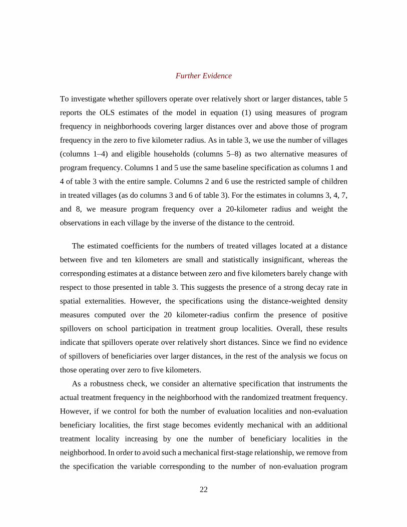
Further Evidence

To investigate whether spillovers operate over relatively short or larger distances, table 5

reports the OLS estimates of the model in equation (1) using measures of program

frequency in neighborhoods covering larger distances over and above those of program

frequency in the zero to five kilometer radius. As in table 3, we use the number of villages

(columns 1–4) and eligible households (columns 5–8) as two alternative measures of

program frequency. Columns 1 and 5 use the same baseline specification as columns 1 and

4 of table 3 with the entire sample. Columns 2 and 6 use the restricted sample of children

in treated villages (as do columns 3 and 6 of table 3). For the estimates in columns 3, 4, 7,

and 8, we measure program frequency over a 20-kilometer radius and weight the

observations in each village by the inverse of the distance to the centroid.

The estimated coefficients for the numbers of treated villages located at a distance

between five and ten kilometers are small and statistically insignificant, whereas the

corresponding estimates at a distance between zero and five kilometers barely change with

respect to those presented in table 3. This suggests the presence of a strong decay rate in

spatial externalities. However, the specifications using the distance-weighted density

measures computed over the 20 kilometer-radius confirm the presence of positive

spillovers on school participation in treatment group localities. Overall, these results

indicate that spillovers operate over relatively short distances. Since we find no evidence

of spillovers of beneficiaries over larger distances, in the rest of the analysis we focus on

those operating over zero to five kilometers.

As a robustness check, we consider an alternative specification that instruments the

actual treatment frequency in the neighborhood with the randomized treatment frequency.

However, if we control for both the number of evaluation localities and non-evaluation

beneficiary localities, the first stage becomes evidently mechanical with an additional

treatment locality increasing by one the number of beneficiary localities in the

neighborhood. In order to avoid such a mechanical first-stage relationship, we remove from

the specification the variable corresponding to the number of non-evaluation program

23

villages (NNE). Note that we still have to control for the number of neighboring evaluation

villages (NE) in order to account for the fact that the identifying variation is non-zero for

42 percent of the evaluation villages (i.e., those that have at least another evaluation village

in their radius of zero to five kilometers) and in order to assure that the exclusion restriction

is valid (because of the correlation across village neighborhoods between NE and NNE).

The corresponding estimation results are reported in table 6. The point estimate of the

first-stage parameter for the effect of an additional treatment group village on

neighborhood treatment density is estimated at 1.43 (column 1). The corresponding t-

statistic is 1.97 and the F test of the excluded instrument is 3.9, which is statistically

significant at the five percent level. The reduced form coefficient for the effect of the

number of treated villages in the zero- to five-kilometer radius on secondary school

enrollment is 0.028 (column 2), which is very much in line with the corresponding estimate

reported in column 1 of table 3. Column 3 reports the IV point estimate of the relationship

between the frequency of neighboring program localities and secondary school enrollment,

which is positive but not significantly different from zero. The IV point estimate has a

smaller magnitude than the OLS one reported in column 2, which reflects the larger-than-

one first-stage relationship and is estimated with more noise due to the reduced statistical

power in this specification.

As a last robustness exercise, we consider alternative measures of program take-up

based on the health component of the program. We use household-level information from

the post-program survey round of October 1998 on the uptake of three screening tests that

form part of the health requirements of the Progresa program: hypertension (blood

pressure test), diabetes (blood sugar test), and cervical cancer (via the PAP smear test).20

20. The household respondents were asked whether or not any household member had been

screened for these conditions in the previous six months. In order to maintain full comparability with

the estimates of program spillover reported in the paper, we estimate at the household-level the

linear model reported in equation (1) in the paper on the same sample that we consider in the main

empirical analysis. Results (available upon request) are very similar in both magnitude and

precision if we instead consider the larger sample of all program-eligible households in October

1998.

24

Table 7 reports the OLS estimates of both own-village treatment effects and the spatial

spillover effects stemming from neighboring program villages on the probability that the

households in the sample comply with the health conditionality of the program. The

estimates reveal the presence of a strong effect of the program on the probability that

eligible households comply with its health requirements, as confirmed by the positive and

large marginal effects associated with the variable indicating whether or not the own village

of residence of the households in the sample received the program.21 The estimated

coefficients of cross-village externalities are reported in columns 1, 3, and 5 of table 7.

These are also positive but not significantly different from zero with the exception of the

specification using the uptake of the blood sugar test as dependent variable (column 3),

which features an estimated externalities coefficient that is significant at the ten percent

level.

We next estimate the heterogenous effect model reported in equation (3). The

corresponding estimates are reported in columns 2, 4, and 6 of table 7. Externalities

coefficients for households residing in treated villages are more precisely estimated and

larger in magnitude when compared to their average counterparts (except for the PAP

smear test) whereas those for control villages cannot be distinguished from zero. An

additional neighboring program village increases compliance with health screening by

roughly ten percent for households who reside in a program village or about half of the

“own-village” treatment effect and a 20–30 percent increase vis-a-vis the corresponding

mean in the control group. These estimates of health spillovers are broadly consistent with

those of the enrollment spillovers reported in table 3 both in terms of incidence (they accrue

exclusively among program participants) and of the magnitude. They are slightly more

imprecise though, possibly due to the smaller sample size resulting from household-level

regressions and one year of program follow-up data.

21. As we note in section 3.1, the fact that program treatment status varies at the village level

implies that such estimates capture both the direct effect of the program as well as the average

indirect effects, which stem from the treatment of other individuals in the same village.

25

III. MECHANISMS

We now use additional information gathered from both program operational surveys and

administrative sources in order to shed some light on the interpretation behind the patterns

uncovered in section 3. The finding of spillovers on school enrollment operating over short

distances supports a simple model of peer effects on program take-up decisions of eligible

households.22 As we do not have measures of the occurrences of interactions of

beneficiaries from different neighboring villages, we cannot report direct evidence of this.

Hence, we conduct several indirect checks for the presence of such interactions. On the

other hand, some spatial variations in the local implementation of the program could also

a priori explain the observed relationship between the local density of the treatment and

program impacts. We thus also test for the presence of such spatial variations in the

implementation of the intervention under study.

Knowledge Spillovers Among Program Participants

In spite of the emphasis placed on informing the potential participants about the objectives,

design, and requirements of the intervention, concerns have been expressed by those

involved in the initial phases of the implementation regarding the effectiveness of the

diffusion of information about the program among targeted households (Adato et al. 2000).

To further corroborate this anecdotal evidence, we use information from an operational

follow-up survey conducted among eligible households in the evaluation treatment-group

villages in May 1999 (i.e., 14 months after the inception of the program). Program

beneficiaries were asked to identify three sets of benefits distributed by Progresa: (i)

scholarships and school supplies; (ii) food stipends and nutritional supplements; and (iii)

preventive healthcare and health check-ups. Most of the respondents who were to receive

the transfers were mothers. While 98 percent of the respondents were able to spontaneously

22. Non-market interactions may affect take-up decisions through two channels: information

and social norms. While conceptually different, these two forms of social behaviors can hardly be

distinguished empirically. We thus broadly refer to the influence of others on individual responses

as peer effects.

26

and correctly mention the nutrition component, only 60 percent correctly identified both

the health and education components. Knowledge of the program components was thus

incomplete in treatment villages at that time.

In such a context of sparse and coarse knowledge about the benefits of the intervention,

information-sharing among potential beneficiaries is likely to have played a role, notably

among the women who are the primary recipients of the transfers and regularly encounter

each other during program operations. When asked, in the same operational follow-up

survey, to mention the most significant changes within their communities, half of the

beneficiaries reported that the program had increased the degree of cooperation among

women.

For further evidence on this, we estimate the effects of spatial spillovers on those

measures of eligible households’ knowledge of the different program components. Table

8 reports the estimates, which are obtained using the model in equation (1) estimated at the

household-level using the October 1998 data. Having one additional neighboring program

village increases by 4.5 and 8.2 percent, respectively, the share of eligible households that

are aware of the education and health components (columns 1 and 2), and has a smaller

and no significant effect on the share of households aware of the nutritional component

(column 3).

Given the evidence of program externalities on school participation decisions presented

in section 3, the observed variations of the knowledge of the education component could

reflect increases in school attendance rather than the presence of peer effect among

potential beneficiaries. Yet, the take-up patterns of the program discussed in section 2.2

make it difficult to interpret the evidence of the knowledge indicators of other program

components (such as health benefits) as purely stemming from corresponding variations in

school enrollment among program-eligible children.

Supply-Side Effects

Areas with higher densities of program participants may have benefited from more efficient

program operations or from improvements in the supply of education or health services,

thereby helping some eligible households to comply with the schooling requirements of

27

the program. A related alternative explanation is that the implementation of the program

may have been more efficient when the number of evaluation treatment group villages in

the neighborhood (rather than the total number of beneficiaries) was higher. While both

notions of implementation scale gains seem a priori reasonable, we argue that they are

unlikely to explain our results.

To examine the presence of differences in implementation and supply, two preliminary

points should be noted. First, any variation in program delivery in a given geographic area

should evenly benefit those program recipients who reside within it. This is at odds with

the evidence reported in column 1 of table 5 that program spillovers appear spatially

concentrated within relatively small areas surrounding the evaluation villages. According

to this line of thought, school supply-side changes would likely affect the enrollment

decisions of both recipients and non-recipients, an idea difficult to reconcile with the

evidence of heterogeneous externalities reported in column 2 of table 3.

Second, we identify spatial spillovers using only the variation in program frequency

generated by the randomized experiment. This variation is small compared to the overall

scale of the program (as seen in table 1, in a given five-kilometer radius there are on average

ten beneficiary villages but only 0.6 evaluation villages, among which 0.4 are assigned to

the treatment group and 0.2 to the control group). Program frequency is thus not much

different in neighborhoods that have more treatment-group villages compared to those that

have more control-group villages, and the resulting infra-marginal changes in the scale of

the program are unlikely to trigger any supply-side efficiency gain.

We next run a battery of complementary tests aimed at detecting the presence of

supply-side responses associated with experimental variations in the frequency of the

treatment in the areas surrounding evaluation villages. We begin with two measures of

implementation efficiency at the village-level. According to qualitative interviews with

beneficiaries, local program staff, school teachers, and health staff (see Adato et al. 2000),

one major source of inefficiency in program delivery was the delays in the delivery of the

form for school attendance monitoring (E1 form), and the associated delays in the payment

of scholarships. First, we use program administrative data on the monetary transfers (for

scholarships and school supplies) delivered to eligible households to compute the number

of months from incorporation until the first disbursements were made to the beneficiary

28

households in treated villages.23 Second, we use information from the operational follow-

up survey in order to construct the share of program recipients in treated villages that

received the E1 form as of May 1999.

In order to maintain full comparability with the estimates of program spillover reported

in the rest of the paper, we estimate at the village-level the linear model reported in equation

(1) using those program implementation measures as dependent variables on the sample of

treated villages that we consider in the main empirical analysis.24 The dependent variables

are time-invariant, and, hence, we match this information with only the first round (1998)

of the data of the program roll-out. As documented in columns 1–3 of table 9, these three

measures of efficiency of program implementation are unrelated to the frequency of the

treatment in the areas surrounding evaluation villages.

We next use the yearly secondary school census in order to construct school supply

aggregate measures for the 358 evaluation neighborhoods in our sample (with both treated

and control villages as centroid), and estimate at the neighborhoodlevel the linear model

reported in equation (1) over the two years of the program roll-out (1998–1999). In all

specifications, we control for the baseline (1997) value of the dependent variable. The OLS

estimates are reported in panel B of table 9, which are very small in magnitude and not

statistically different from zero.

23. While food stipends were distributed to all villages assigned to the treatment group at the

same time in March 1998, only 56 percent of the those localities received the first scholarship

transfer in March 1998; 36 percent received them two months later, and the remaining eight percent

six months or more after incorporation into the program. These administrative delays appear

concentrated in some regions, notably in the states of Queretaro and San Luis Potosi. As a further

check, we have re-estimated equation (1) without those two states. Results (available upon

request) are very similar to those reported in table 3.

24. Results (available upon request) barely change when we consider instead the entire sample

of 320 treated villages. Due to a few missing values in the additional data sources that we employ,

we lose some village-level observations in the regressions displayed in panel A of table 2: three

villages for scholarship disbursements, four villages for school supply disbursements, and seven

villages for the receipt of the school attendance (E1) form.

29

IV. CONCLUSION

We examined, in the context of the Progresa-Oportunidades conditional cash transfer

program, whether or not the take-up of the schooling component of the program is

influenced by the presence of other beneficiaries in areas comprising several villages. We

found evidence of positive spillovers within networks of beneficiaries spanning those

areas. A higher local frequency of program beneficiaries increases the take-up of the

scholarships for secondary schooling offered by the program and, accordingly, school

enrollment at that level. In contrast, these effects do not affect the schooling decisions of

households in the control-group villages that were not yet incorporated into the program.

To better understand our findings, we tested and found suggestive evidence for the

presence of knowledge spillovers among program-eligible households. While we could not

directly test for the presence of social interactions, we found that higher treatment densities

in the neighborhoods were associated with increased knowledge among eligible

households of the schooling and health components of the program. We also tested the

alternative hypothesis that the spillover effect that we estimate instead reflects

heterogeneities in direct treatment impacts due to spatial variations in the implementation

of the program. The evidence we obtained is not consistent with this interpretation of our

findings.

Spillover effects on program take-up have implications for the design and

implementation of social policies in developing countries. The magnitude of the estimated

effect suggests that there can be large gains from the spatial concentration of the target

population of an intervention as local networks of potential beneficiaries can act as social

multipliers in the take-up of the proposed benefits. Spillover effects also have implications

for the evaluation of social policy interventions, notably in settings where a program is

implemented over an extended area and treatment frequency is high. In particular,

capturing those effects across villages so as to recover impact evaluation parameters that

incorporate spillovers requires the analysis of the impacts of the program at the level of

relatively large geographical areas or clusters. The feasibility of this option critically hinges

upon the scale of the program that is being evaluated, and statistical power reasons may

push the researcher to opt for a narrower definition of the evaluation clusters. These

30

considerations can be particularly important for policy interventions that are evaluated at

scale, a setting which likely differs from the evaluation of small pilot programs.

REFERENCES

Adato, M., D. Coady, and M. Ruel. 2000. “An operations evaluation of progresa from the

perspective of beneficiaries, promotoras, school directors, and health staff.” Technical

report, International Food Policy Research Institute, Washington, DC.

Aizer, A., and J. Currie. 2004). ”Networks or neighborhoods? correlations in the use of

publicly-funded maternity care in California.” Journal of Public Economics 88

(12): 2573–85.

Akerlof, G.A. 1997. “Social distance and social decisions.” Econometrica 65 (5): 1005–

28.

Angelucci, M., and G. De Giorgi. 2009. ”Indirect effects of an aid program: How do cash

transfers affect ineligibles’ consumption?” American Economic Review 99 (1): 486–

508.

Angelucci, M., G. De Giorgi, M.A. Rangel, and I. Rasul. 2010. ”Family networks and

school enrollment: Evidence from a randomized social experiment.” Journal of

Public Economics 94 (3-4): 197–221.

Angelucci, M., G. De Giorgi, and I. Rasul. 2015. Resource sharing within family

networks: insurance and investment. Working paper.

Baird, S., J.A. Bohren, C. McIntosh, and B. Ozler. 2015. Designing Experiments to

Measure Spillover Effects, working paper 15-021, Penn Institute for Economic

Research. University of Pennsylvania, Philadelphia, PA.

Banerjee, A., E. Duflo, R. Glennerster, and K. Dhruva. 2010. ”Improving immunization

coverage in rural India: A clustered randomized controlled evaluation of

immunization campaigns with and without incentives.” BMJ 340:c2553.

Bertrand, M., E.F.P. Luttmer, and S. Mullainathan. 2000.”Network effects and welfare

cultures.” Quarterly Journal of Economics 115 (3), 1019–55.

Bobonis, G.J., and F. Finan. 2009. ”Neighborhood peer effects in secondary school

enrollment decisions.” Review of Economics and Statistics 91 (4): 695–716.

31

Brock, W.A. and S.N. Durlauf. 2001. ”Discrete Choice with Social Interactions.” Review

of Economic Studies 68 (2): 235–60.

Crepon, B., E. Duflo, M. Gurgand, R. Rathelot, and P. Zamora. 2013. ”Do labor market

policies have displacement effects? Evidence from a clustered randomized

experiment.” Quarterly Journal of Economics 128 (2): 531–80.

Daponte, B.O., S. Sanders, and L. Taylor. 1999. “Why do low-income households not use

food stamps? Evidence from an experiment.” Journal of Human Resources 34

(3): 612–28.

Duflo, E., and E. Saez. 2003. ”The role of information and social interactions in

retirement plan decisions: Evidence from a randomized experiment.” Quarterly

Journal of Economics 118 (3): 815–42.

Fiszbein, A., and N. Schady. 2009. Conditional Cash Transfers. Reducing Present and

Future Poverty. The World Bank, Washington, DC.

Glaeser, E.L., and J. Scheinkman. 2000. Non-Market Interactions, NBER working papers

8053, National Bureau of Economic Research, Inc.

Glewwe, P., and M. Kremer. 2006. Schools, teachers, and education outcomes in

developing countries, Vol. 2 of Handbook of the Economics of Education. Elsevier,

chapter 16, 945–1017.

Ichino, N., and M. Schundeln. 2012. ”Deterring or displacing electoral irregularities?

Spillover effects of observers in a randomized field experiment in Ghana.” Journal of

Politics 74: 292–307.

Kuhn, P., P. Kooreman, A. Soetevent, and A. Kapteyn. 2011. ”The effects of lottery

prizes on winners and their neighbors: Evidence from the Dutch postcode lottery.”

American Economic Review 101 (5): 2226–47.

Lalive, R., and M.A. Cattaneo. 2009. ”Social interactions and schooling decisions.”

Review of Economics and Statistics 91 (3): 457–77.

Miguel, E., and M. Kremer. 2004. ”Worms: Identifying impacts on education and health

in the presence of treatment externalities.” Econometrica 72 (1): 159–217.

Moffitt, R.A. 2001. Policy Interventions, Low Level Equilibria, and Social Interactions.

Cambridge, MA: MIT Press, 45–82.

32

Parker, S.W., L. Rubalcava, and G. Teruel. 2008. “Evaluating Conditional Schooling and

Health Programs.” Vol. 4 of Handbook of Development Economics. Elsevier,

chapter 62: 3963–4035.

Schultz, T.P. .2004. ”School subsidies for the poor: Evaluating the Mexican progresa

poverty program.” Journal of Development Economics 74 (1): 199–250.

33

FIGURES AND TABLES

FIGURE 1. Program Coverage (1998-1999)

Notes: This figure reports the geographic locations of the villages targeted by the program during

the period 1998–1999 in the seven central states of Mexico in which the evaluation of the program

took place. The quadrant in the upper right hand corner displays a close-up view of a region in the

state of Michoacan in which the size of the markers has been adjusted for the relative population

size, and five-kilometer radiuses are displayed around each evaluation village.

Source: list of localities receiving the Progresa-Oportunidades at end of 1998 and 1999, list of

localities selected in the treatment and control group of the randomized evaluation, and 2000

population census.

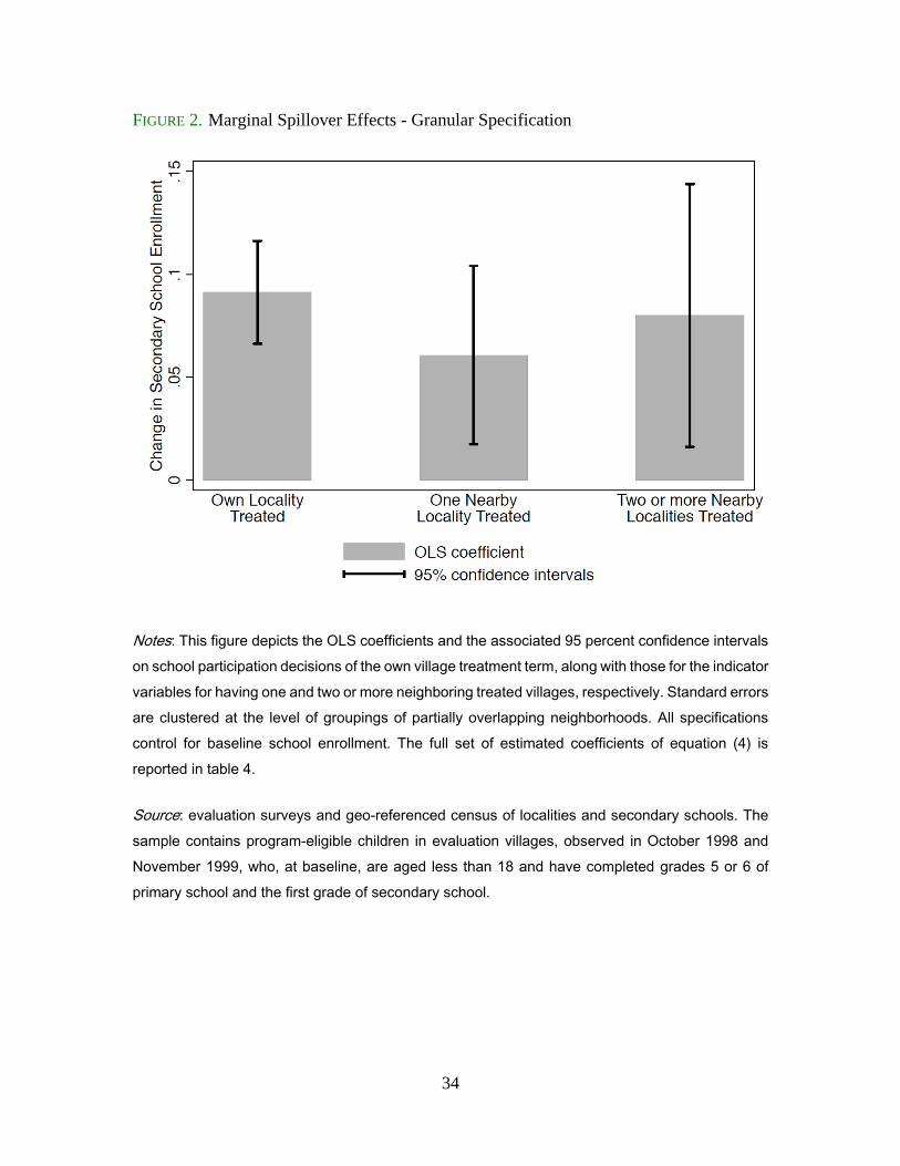
34

FIGURE 2. Marginal Spillover Effects - Granular Specification

Notes: This figure depicts the OLS coefficients and the associated 95 percent confidence intervals

on school participation decisions of the own village treatment term, along with those for the indicator

variables for having one and two or more neighboring treated villages, respectively. Standard errors

are clustered at the level of groupings of partially overlapping neighborhoods. All specifications

control for baseline school enrollment. The full set of estimated coefficients of equation (4) is

reported in table 4.

Source: evaluation surveys and geo-referenced census of localities and secondary schools. The

sample contains program-eligible children in evaluation villages, observed in October 1998 and

November 1999, who, at baseline, are aged less than 18 and have completed grades 5 or 6 of

primary school and the first grade of secondary school.

35

36

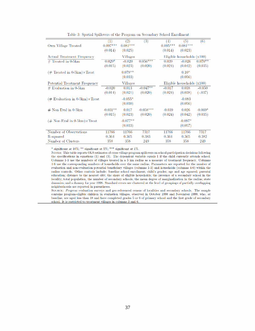
37

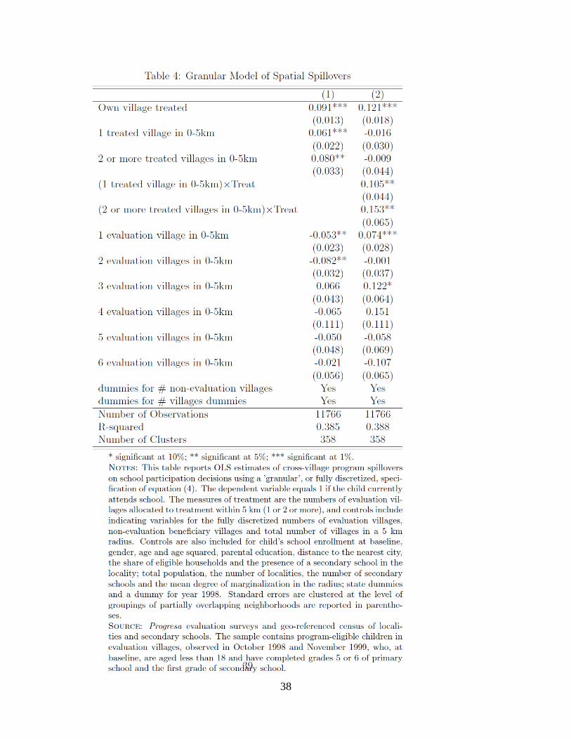
38

39

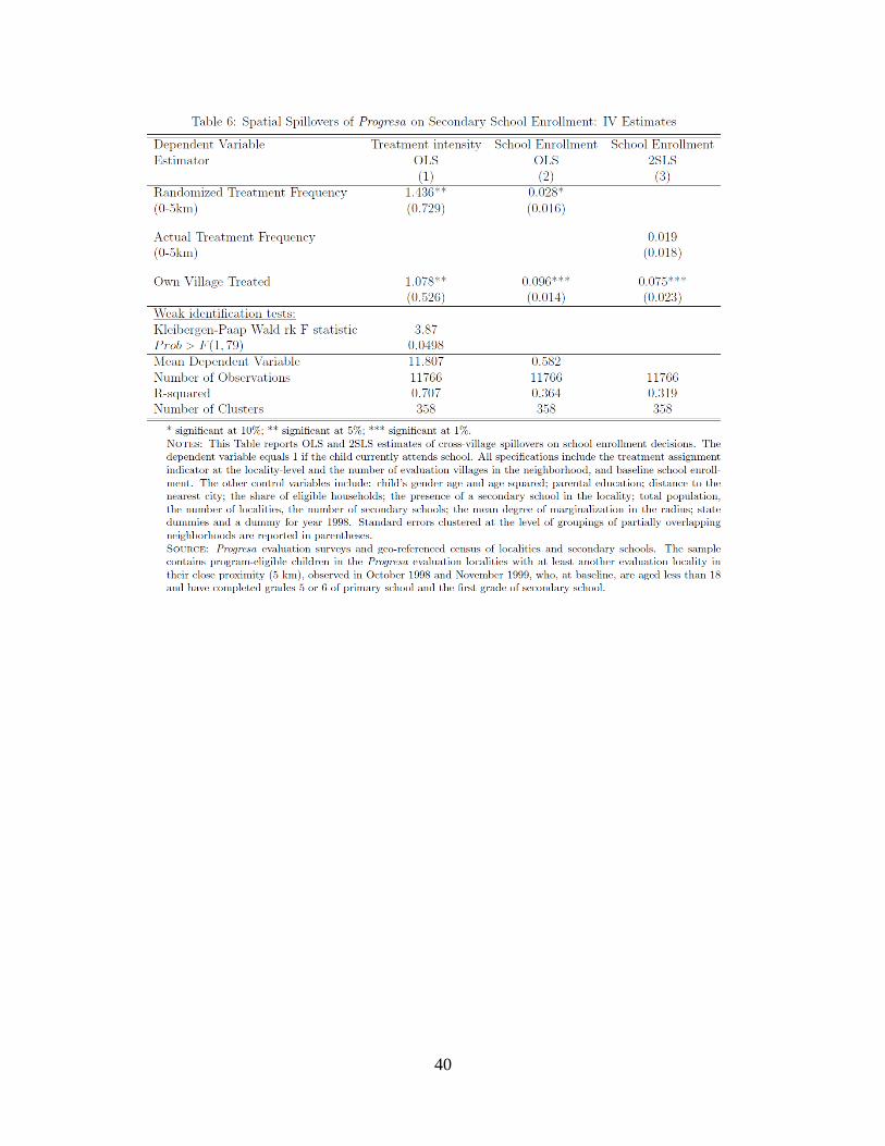
40

41

42

43

Neighborhood Effects in Integrated Social PoliciesSupplemental Appendix

Matteo Bobba∗ Jeremie Gignoux†

S1 Randomness of the Evaluation Sample

We hereby provide the english translation for a few extracts of an official document from theoriginal evaluation of the program (Progresa, 1997), which clearly suggest that the evaluationsample was indeed selected randomly among the set of the program eligible localities in theseven Mexican States in which the program was initially implemented.

[...]The evaluation sample (cf. BASAL y CONTROL) is constituted of rural(i.e. 50-4,999 inhabitants) and marginalized (i.e. high or very high values ofan underlying proxy-mean poverty score) localities with access to primary andsecondary schools that are located in Progresa catchment areas in the States ofGuerrero, Hidalgo, Michoacan, Puebla, Queretaro, San Luis Potosı and Veracruz.

[...]The sample was randomly drawn from the population of those program eligiblelocalities scheduled to be incorporated in 1997, after stratification by geographicregion (which roughly coincide with States) and population size.

In the regression analysis discussed in the paper, individual school participation decisionsafter the program takes place (1998-1999) are affected by the local frequency of program in-corporated villages over the same period in the areas surroundings their villages of residence.Hence, beyond the presumed randomness of the evaluation sample vis-a-vis the villages thatwere incorporated during the baseline of the program evaluation (1997), we are also inter-ested in assessing the extent to which the evaluation villages are similar to those that wereincorporated in the program during the subsequent phases of the roll-out of the interventionin rural areas. Basic socio-demographic variables extracted from the 2000 Mexican popu-lation census indicate that localities that are lately incorporated into the program are onaverage larger and less marginalized (see Panel A of Table S1.1). However, the differencesin means between incorporation phases are largely attenuated once we restrict the sampleto those localities that are situated in 5km neighborhoods (as defined in the paper) of theevaluation localities (see panel B of Table S1.1).

∗Toulouse School of Economics, University of Toulouse Capitole, 21 Allee de Brienne 31000 ToulouseFrance. E-mail: matteo.bobba@tse-fr.eu.†French National Institute for Agricultural Research and Paris School of Economics, 48 boulevard Jourdan

75014 Paris France. E-mail: jeremie.gignoux@psemail.eu.

1

Table S1.1: Socio-Demographics Characteristics and the Phase of Program Incorporation

Year 1997 1998 1999Mean Std. Dev. Mean Std. Dev. Mean Std. Dev.

(1) (2) (3) (4) (5) (6)

Panel A: All Localities in the Seven States in which the Program Evaluation Took Place

Size size N=2,249 N=11,987 N=6,124

Poverty mean-score 0.63 0.65 0.61 0.69 0.09 0.88Nb of Households 70.17 94.71 73.74 99.91 91.35 171.17Population (age≤5) 59.58 83.63 63.99 88.98 71.93 141.81Population (6≤age<15) 91.47 124.62 96.64 129.09 108.20 204.99Population (age≥15) 202.9 280.1 207.5 279.6 258.1 489.5Presence of secondary school 0.20 0.40 0.19 0.40 0.22 0.42% Literate (age≥15) 0.69 0.13 0.70 0.14 0.75 0.14% Children in School (6≤age<15) 0.90 0.09 0.88 0.10 0.87 0.12Altitude (meters above see level) 940.2 683.2 1092.7 855.6 1238.5 886.6% Population in Workforce 0.43 0.11 0.40 0.13 0.39 0.13

Panel B: Only Localities in a 5-km Neighborhood of the Evaluation Sample

Size size N=717 N=3,048 N=829

Poverty mean-score 0.66 0.64 0.67 0.72 0.16 0.99Nb of Households 68.32 87.73 63.67 74.21 76.63 200.37Population (age≤5) 57.78 78.32 55.83 68.24 60.02 149.05Population (6≤age<15) 90.12 117.9 84.27 97.85 91.07 214.4Population (age≥15) 198.3 261.4 180.9 211.1 216.0 568.6Presence of secondary school 0.19 0.40 0.17 0.37 0.20 0.40% Literate (age≥15) 0.68 0.13 0.68 0.15 0.72 0.17% Children in School (6≤age<15) 0.90 0.10 0.88 0.10 0.88 0.13Altitude (meters above see-level) 900.1 682.8 1215.9 842.9 1448.8 833.4% Population in Workforce 0.44 0.12 0.42 0.14 0.42 0.14

Note: Both Samples of Panel A and Panel B include the 320 evaluation localities that were randomlyassigned to the treatment group.

Table S1.2 provides a direct comparison between evaluation localities and the non-evaluation program beneficiary localities in the seven Mexican States from which the eval-uation sample was drawn and over the period 1997-1999 (see columns 1 and 2). Column 3reports the t-statistics of the test of no differences in locality characteristics after controllingfor population strata and State fixed effects (as well as a joint F-test) and finds the presenceof some unbalances in a few socio-demographic characteristics. In Column 4 we further re-strict the comparison within the neighboring localities of each evaluation cluster and do notfind evidence of any significant difference between the two samples.

To wrap up, in spite of the random assignment of evaluation villages in 1997, theremay be some unbalancedness between the evaluation sample and the non-evaluation sample

2

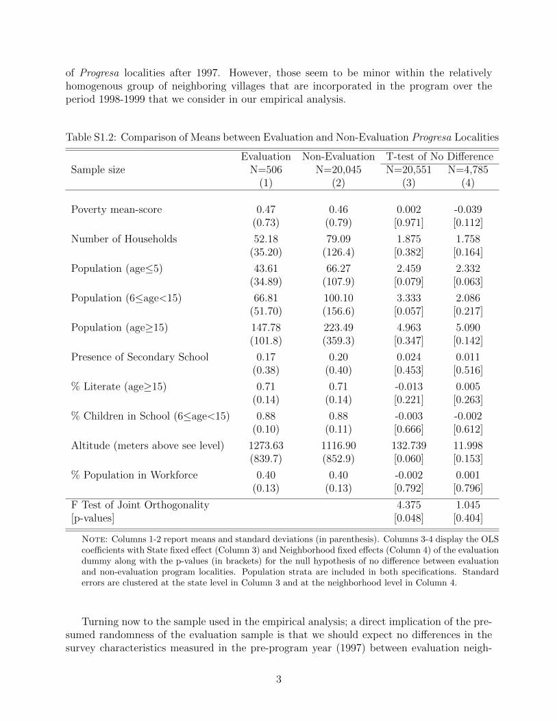
of Progresa localities after 1997. However, those seem to be minor within the relativelyhomogenous group of neighboring villages that are incorporated in the program over theperiod 1998-1999 that we consider in our empirical analysis.

Table S1.2: Comparison of Means between Evaluation and Non-Evaluation Progresa Localities

Evaluation Non-Evaluation T-test of No DifferenceSample size N=506 N=20,045 N=20,551 N=4,785

(1) (2) (3) (4)

Poverty mean-score 0.47 0.46 0.002 -0.039(0.73) (0.79) [0.971] [0.112]

Number of Households 52.18 79.09 1.875 1.758(35.20) (126.4) [0.382] [0.164]

Population (age≤5) 43.61 66.27 2.459 2.332(34.89) (107.9) [0.079] [0.063]

Population (6≤age<15) 66.81 100.10 3.333 2.086(51.70) (156.6) [0.057] [0.217]

Population (age≥15) 147.78 223.49 4.963 5.090(101.8) (359.3) [0.347] [0.142]

Presence of Secondary School 0.17 0.20 0.024 0.011(0.38) (0.40) [0.453] [0.516]

% Literate (age≥15) 0.71 0.71 -0.013 0.005(0.14) (0.14) [0.221] [0.263]

% Children in School (6≤age<15) 0.88 0.88 -0.003 -0.002(0.10) (0.11) [0.666] [0.612]

Altitude (meters above see level) 1273.63 1116.90 132.739 11.998(839.7) (852.9) [0.060] [0.153]

% Population in Workforce 0.40 0.40 -0.002 0.001(0.13) (0.13) [0.792] [0.796]

F Test of Joint Orthogonality 4.375 1.045[p-values] [0.048] [0.404]

Note: Columns 1-2 report means and standard deviations (in parenthesis). Columns 3-4 display the OLScoefficients with State fixed effect (Column 3) and Neighborhood fixed effects (Column 4) of the evaluationdummy along with the p-values (in brackets) for the null hypothesis of no difference between evaluationand non-evaluation program localities. Population strata are included in both specifications. Standarderrors are clustered at the state level in Column 3 and at the neighborhood level in Column 4.

Turning now to the sample used in the empirical analysis; a direct implication of the pre-sumed randomness of the evaluation sample is that we should expect no differences in thesurvey characteristics measured in the pre-program year (1997) between evaluation neigh-

3

borhoods with a different number of non-centroid evaluation villages after netting out theindependent effect of the local frequency of neighboring non-evaluation localities. A simplecomparison of means between evaluation neighborhoods with and without non-centroid eval-uation villages is shown in columns 1 and 2 of Table S1.3. Column 3 reports the effects ofthe number of evaluation villages after controlling for the number of non-evaluation villagesin the neighborhood. Overall, the local frequency of evaluation localities in the neighbor-hoods of the 506 localities that form part to the Progresa evaluation sample does not seemto be correlated with pre-program observable characteristics at the individual, locality andneighborhood-level. This confirms that the set of evaluation localities is a random subsampleof beneficiary localities incorporated after late 1997.

4

Table S1.3: Baseline Characteristics within the Evaluation Localities

Neighborhood No Evaluation Some Evaluation OLS Coefficient ofLocalities Localities Number of Eval (NE

j,5)

(1) (2) (3)

School Enrollment 0.64 0.64 0.004(0.48) (0.48) [0.647]

Individual and HH Characteristics

Age 14.52 14.53 -0.016(2.02) (2.06) [0.513]

Female (dummy) 0.50 0.51 0.002(0.50) (0.50) [0.729]

Mother Education (years) 2.36 2.36 0.077(2.33) (2.35) [0.396]

Father Education (years) 2.20 2.25 0.085(2.21) (2.30) [0.139]

Centroid Village Characteristics

Share of Program Eligible HHs 0.58 0.60 -0.008(0.20) (0.19) [0.409]

Presence of Secondary School 0.26 0.24 -0.006(0.44) (0.43) [0.789]

Distance to Nearest City (Km) 106.4 102.9 4.191(40.45) (45.59) [0.255]

Neighborhood (radius=5km) Characteristics

Number of Secondary Schools 2.88 3.19 0.037(2.19) (1.91) [0.800]

Poverty mean-score 0.41 0.57 0.042(0.56) (0.54) [0.151]

Number of Localities (any) 21.03 25.15 -0.181(14.00) (11.21) [0.798]

Population density 5.99 8.41 0.572(6.54) (11.44) [0.575]

F Test of Joint Orthogonality 1.099[p-values] [0.357]

Note: Columns 1-2 report means and standard deviations (in parenthesis). Column 3 displays theOLS coefficients of the number of neighboring (within 5km) evaluation localities after controlling forthe number of neighboring (within 5km) non-evaluation Progresa localities along with the associatedp-values (in brackets). State fixed effects are included in all specifications. Standard errors areclustered at the level of groupings of partially overlapping neighborhoods.

5

S2 Consistency of the OLS coefficients When One or

More Regressor is Endogenous

A general writing of the linear regression model we consider is

y = x1β1 + x2β2 + u

where x2 is a matrix of endogenous explanatory variables, i.e. E(x′2u) 6= 0 and x1 is a matrixof explanatory variables that are exogenous, i.e. i.e. E(x′1u) = 0. β1 and β2 are (column)vectors of coefficients and u is a vector of the error terms.

In our specific case, x2 is the number of potential beneficiary villages NP , while x1 is thenumber of actual beneficiary villages NB. While NB is correlated with treatment densityand hence potentially associated with unobserved determinants of outcomes captured by theresidual u in an unconditional model, it is not anymore when we control for NP . This isbecause the residual variation in NB is then solely determined by the random number oftreatment group villages in the neighborhood. The model we estimate is formally similar tothe general model above, as the same estimates can be obtained using the variables NC andNP , and NC is exogenous while NP is endogenous; we indeed have:

y = β1NB + β2N

P + u = β1(NP −NC) + β2N

P + u = −β1NC + (β1 + β2)NP + u

Using the partitioned matrix notation, the vector of OLS coefficients is given by(β1β2

)=

(x′1x1 x′1x2x′2x1 x′2x2

)−1(x′1x′2

)u

Since x2 is random conditional on x1, it follows that the two set of explanatory variables areuncorrelated with each others: E(x′1x2) = 0. Hence, the variance V (x1, x2) of the full set ofcovariates in the right-hand side term converges asymptotically to(

x′1x1 x′1x2x′2x1 x′2x2

)→

(E(x′1x1) 0

0 E(x′2x2)

)Using the independence of x2 from u, the product of the last two terms converges to(

x′1x′2

)u→

(E(x′1u)

0

)So the vector of coefficients converges asymptotically to(

β1β2

)→

(β1β2

)+

(E(x′1x1)

−1E(x′1u)0

)To summarize, the OLS coefficients β2 are consistent estimates of the marginal effects of theexogenous variables, β2. On the other hand, the OLS coefficients on the endogenous variablesβ1 are biased, due for instance to omitted variables, but this bias does not contaminate the

6

coefficients estimated for the exogenous variables to the extent that those are uncorrelatedwith the endogenous variables. In our setting, this is likely the case because the partialvariation in NB (i.e. after netting out the effect of NP ) solely captures the randomizedallocation into treatment of evaluation localities.

Additional References

Progresa (1997). “Nota Tecnica: Diseno Muestra Basal y Control”, Technical Note.

7