Embed Size (px)
Citation preview

Neighborhood Air Toxics Modeling Project for
Houston and Corpus Christi Case # 2:11-MC-00044
Phase 1B
Monitoring Network Extension
Annual Progress Report for the Period
October 1, 2013 through September 30, 2014
Submitted to
The Honorable Janis Graham Jack United States District Court for the Southern District of Texas
Corpus Christi, Texas
Mr. John L. Jones United States Environmental Protection Agency, Region 6
Dallas, Texas
Ms. Susan Clewis Texas Commission on Environmental Quality, Region 14
Corpus Christi, Texas
Submitted by
David Allen, Ph.D. Principal Investigator
Center for Energy and Environmental Resources The University of Texas at Austin
10100 Burnet Road, Bldg 133 (R7100) Austin, TX 78758
512/475-7842 [email protected]
March 30, 2015
1

ANNUAL PROGRESS REPORT TO THE U.S. DISTRICT COURT
FOR THE NEIGHBORHOOD AIR TOXICS MODELING PROJECT
FOR HOUSTON AND CORPUS CHRISTI PHASE 1B: MONITORING NETWORK EXTENSION
October 1, 2013 through September 30, 2014
INTRODUCTION On February 1, 2008, the United States District Court entered an Order (D.E. 981, Order (pp.1, 7-11)) regarding unclaimed settlement funds in Lease Oil Antitrust Litigation (No.11) Docket No. MDL No. 1206. The Court requested a detailed project proposal from Dr. David Allen, the Gertz Regents Professor in Chemical Engineering and the Director of the Center for Energy and Environmental Resources at The University of Texas at Austin (UT Austin), regarding the use of $9,643,134.80 in the Settlement Fund. The proposal was for a project titled “Neighborhood Air Toxics Modeling Project for Houston and Corpus Christi” (hereinafter “Air Toxics Project”). The Air Toxics Project was proposed in two stages. In Stage 1, UT Austin was to develop, apply, demonstrate and make publicly available, neighborhood-scale air quality modeling tools for toxic air pollutants in Corpus Christi, Texas (Phase 1A) and extend the operating life of the air quality monitoring network in Corpus Christi, Texas (Phase 1B). The ambient monitoring results from Stage 1 Phase 1B were to be used in synergy with the neighborhood-scale models to improve the understanding of emissions and the spatial distribution of air toxics in the region. On February 21, 2008, the United States District Court for the Southern District of Texas issued an order to the Clerk of the Court to distribute funds in the amount of $4,586,014.92, plus accrued interest, to UT Austin for the purposes of implementing Stage 1 of the Air Toxics Project as described in the detailed proposal submitted to the Court by UT Austin on February 15, 2008 (D.E. 998). Under the Order to Distribute Funds in MDL No. 1206, on March 3, 2008, at the direction of the Settlement Administrator, $4,602,598.66 was disbursed to UT Austin for Stage 1 of the Project. This amount includes the interest accrued prior to distribution from the MDL No. 1206 Settlement Fund. In Stage 2, subject to the availability of funds, it was planned that UT Austin would extend the modeling to the Houston, Texas ship channel region, develop a mobile monitoring station that could be deployed in Corpus Christi and in other regions of Texas and/or further extend the operating life of the existing stationary network in the same or a modified spatial configuration. Based on the decision of the U.S. Court of Appeals for the 5th Circuit on June 27, 2011, UT Austin will not be receiving the Stage 2 funding at any point in the future. Further, work on the modeling portion of Stage 1 (Phase 1A) was completed June 30, 2011. Hence, all future progress reports will describe only work on Stage 1 Phase 1B. The air quality monitoring network was originally authorized on October 1, 2003, when the United States District Court for the Southern District of Texas issued an order to the Clerk of the Court to distribute funds in the amount of $6,700,000, plus interest accrued, to UT Austin to
2

implement the court ordered condition of probation (COCP) project Corpus Christi Air Monitoring and Surveillance Camera Installation and Operation (Project). Those funds have been expended. Funding for the air quality monitoring network originally created for the COCP Project is now provided through Stage 1 Phase 1B of the Air Toxics Project. A. MONITORING SITES AND EQUIPMENT INSTALLED The COCP consists of a network of six (6) continuous ambient air monitoring stations (CAMSs) as shown in the map below in Figure 1 with air monitoring instruments and surveillance camera equipment as shown in Table 1, on page 4. Sulfur dioxide (SO2), hydrogen sulfide (H2S), hydrocarbon species with one carbon atom to 11 carbon atoms, and meteorological parameters are measured at each CAMS. Each CAMS is identified with a number as shown in Table 1 and often shown on maps with, for example, “CAMS 633” abbreviated as “C633”. Speciated hydrocarbon chemicals may be measured either by an automated chromatogram instrument (auto-GC) or sampled in canisters and quantified later in a laboratory. Methane and the total sum of all other common two carbon atom to 11 carbon atom hydrocarbons (unspeciated) – total nonmethane hydrocarbon (TNMHC) – are measured at four sites. Figure 1. Corpus Christi Monitoring Sites, “X” marks a UT site terminated in 2012
6 Current UT monitoring sites at yellow thumbtacks 7 TCEQ monitoring sites at blue thumbtacks
3

Table 1. Schedule of UT Air Monitoring Sites, Locations and Major Instrumentation
TCEQ CAMS# Description of Site Location
Monitoring Equipment Auto GC
TNMHC (T) / Canister (C)
H2S & SO2
Met Station Camera
634
Oak Park Recreation Center (OAK) Mar
2005 to date
C: Dec 2004 to Feb 2009
T: Dec 2004 to Apr 2012
Dec
2004 to date
629 Grain Elevator @ Port of Corpus Christi (CCG) T&C: Dec
2004 to date
Dec 2004 to
date
Dec 2004 to
date
630 J. I. Hailey Site @ Port of Corpus Christi (JIH) T&C: Dec
2004 to date
Dec 2004 to
date
Dec 2004 to
date
635 TCEQ Monitoring Site C199 @ Dona Park (DPK) T&C: Dec
2004 to date
Dec 2004 to
date
Dec 2004 to
date
Jan 2005 to date
632 Off Up River Road on Flint Hills Resources Easement (FHR)
T&C: Dec 2004 to date
Dec 2004 to
date
Dec 2004 to
date
633
Solar Estates Park at end of Sunshine Road (SOE) Mar
2005 to date
C: Dec 2004 to Feb 2009
T: Dec 2004 to Apr 2012
Dec 2004 to
date
Dec 2004 to
date
Jan 2005 to date
631
Port of Corpus Christi on West End of CC Inner Harbor (WEH) (site terminated)
T&C: Dec 2004 to May
2012
Dec 2004 to
May 2012
Dec 2004 to
May 2012
Legend CAMS continuous ambient monitoring station Auto GC automated gas chromatograph
TNMHC total non-methane hydrocarbon analyzer (all except CAMS 634 & 633 also have canister hydrocarbon samplers)
H2S hydrogen sulfide analyzer SO2 sulfur dioxide analyzer
Met Station meteorology station consisting of measurement instruments for wind speed, wind direction, ambient air temperature and relative humidity
Camera surveillance camera B. DATA ANALYSIS As noted in Table 1, above, the monitoring network provides measurements of hydrocarbons, sulfur dioxide, hydrogen sulfide, and meteorology. Provided below are brief findings from the monitoring network during FY2014 (October 1, 2013 through September 30, 2014). More details are available in Appendix A, on pages 09 through 40.
4

Results of Canister Sampling At four of the six monitoring sites, an ambient air sample may be collected in a canister for subsequent laboratory analysis if a sustained level of elevated concentrations of total nonmethane hydrocarbons (TNMHC) has been measured, i.e., concentration greater than 2000 parts per billion carbon (ppbC) for longer than 15 minutes. During FY2014, a total of 28 usable canister samples were collected in the Corpus Christi network due to sustained levels of elevated concentrations of TNMHC. One measured hydrocarbon concentration on January 11, 2014 was higher than the TCEQ’s Air Monitoring Comparison Value (AMCV) odor threshold, but no other measurements exceeded their respective AMCV. Summary of Sulfur Species Monitoring EPA established a new federal standard for sulfur dioxide (SO2) in 2010. No exceedances of the State of Texas standards for (SO2) and (H2S) were measured this fiscal year, but one exceedance of the federal SO2 standard was measured. A mid-2012 change in regulations may have resulted in lowered SO2 emission rates from one source category – ships at dockside in the Ship Channel. Overall, SO2 concentrations have declined significantly at most sites. Summary of Continuous Hydrocarbon Species Monitoring No short-term concentrations or long-term average concentrations were measured that were greater than the State of Texas air monitoring comparison values for benzene, 1,3-butadiene, or any other hydrocarbons this fiscal year. Most species measured have lower annual averages in the most recent six years, compared to the project’s first three years. However, several alkane species are showing recent increases in mean concentration trends over the past three years. Trends in Benzene Concentrations in Residential Areas Because of a high level of concern with benzene, a known carcinogen, this compound is given special attention. An analysis of the benzene data shows concentrations in FY 2014 were similar to the six previous years, and significantly lower than in FY 2005 – FY 2007. C. ADVISORY BOARD The Advisory Board for the Corpus Christi Air Monitoring and Surveillance Camera Project is a voluntary Board that consists of seven members. The members and their representation on the Board follow: Ms. Gretchen Arnold Local Air Quality Issues and Board Spokesperson Dr. Eugene Billiot Technical Support to the Board - Instrumentation Ms. Sharon Lewis City of Corpus Christi Dr. William Burgin Local Public Health - Local Air Quality Issues Ms. Joyce Jarmon Community Representation Dr. Glen Kost Community Representation Mr. Christopher Schulz Community Representation Two meetings of the Advisory Board were held during this year of the project. Both meetings were held on the campus of Texas A&M University in Corpus Christi, Texas. In addition to the
5

advisory board meetings Dr. Sullivan also gave a talk to the Long-term Health Workgroup on January 8, 2014, to discuss our activities. He also submitted a proposal to EPA for another air quality project in Corpus Christi involving use of community-based low cost portable air pollution monitors (which was not funded). Highlights from these meetings follow:
April 3, 2014 Meeting
• Dr. Dave Sullivan gave an update on and analysis of monitoring data collected by the Project for the past 9 years. As of April 3, 2014, the project has now collected 9 years of monitoring data.
• Dr. Kost asked if there was only one report of elevated benzene in FY 2013. Dr. Sullivan reported that yes, the Port Grain site had triggered a canister sample of elevated benzene on Oct. 23, 2012. Dr. Kost inquired if the canister was triggered due to emissions from the ships. Dr. Sullivan reported that not due to ships but quite possibly a release from an above ground storage tank in the area. However, he was not sure what chemical was released. Mr. Chris Owens asked how long the sampling duration was. Dr. Sullivan responded that the duration of the sampling was 20 minutes.
• Dr. Sullivan noted that there was an uptick in propane and ethane in FY 2013, with
higher concentrations associated with westerly and northerly winds. Dr. Kost inquired if it was possibly due to either new pipelines or new storage tanks in the area. Ms. Gretchen Arnold mentioned that there were four workers that were hurt in a flash fire at an Enterprise Products natural gas processing plant. Dr. Kost mentioned that residents of Dona Park were concerned with this incident. Dr. Sullivan will request information from the Railroad Commission. Ms. Rosario Torres (TCEQ), also mentioned that she will follow up with the Railroad Commission. Dr. Sullivan asked the Advisory Board members to send any specific questions to him and he will try to find answers. Dr. Sullivan will get back to the Advisory Board with more information after further study.
• Dr. Sullivan mentioned that there were several upticks in the SO2 concentration between October 1, 2013, and December 20, 2013, at the Solar Estates monitoring site but it leveled off at zero through 3/04/14. Mr. Owens mentioned that a bleaching agent was a possible source that was used in the stacks at the refinery to control odors. The hours of the elevated SO2 concentrations were noted during the work day during either early morning or late afternoon. The TCEQ had contacted the company and was told that the company had not changed any of the cleaning chemicals, nor were any scrubber solutions changed. Neither the TCEQ nor the company has any idea what change caused the uptick in SO2 concentrations. Dr. Sullivan will continue to look into this.
December 10, 2013 Meeting
• Project manager Vincent Torres presented an update on the financial status of the project,
estimate months of operation of the project remaining, and proposed plans for the decommissioning of the project. Mr. Torres stated that UT anticipates the funding will allow continuation of all the monitoring activities through January 2016. At that time
6

decommissioning for the sites would commence. This projection is an approximation based on the current financial status and the assumption that no unanticipated major expenses are incurred.
• Dr. Dave Sullivan gave an update on and analysis of monitoring data collected by the project for the past 9 years. As of December 10, 2013, the project has now collected 8.5 to 9 years of monitoring data.
• Dr. Kost asked if there is anyway UT can evaluate the influence the trucking industry has
on the air quality measurements currently being collected at the Project’s air monitoring sites. Dr. Sullivan mentioned that trucks are getting cleaner. Mr. Chris Owen, (TCEQ) pointed out that the TCEQ TERP Grant Program is available to the trucking industry to purchase new diesel equipment. The TCEQ actively publicizes the TERP Grant Program.
• Mr. Joe Montoya (TCEQ), commented on the Trajectory Tool developed by UT under
TCEQ-SEP funding. He told the attendees that the Trajectory Tool is used by the TCEQ every day. He wanted the group to know that the tool is very useful for back trajectory projections, and it is very useful for forward trajectory projections as well. Support for this tool will end when monitoring operations cease January 2016.
• Dr. Kost inquired if Dr. Sullivan has been given a map of all of the new pipeline activity
in the Corpus Christi area. Dr. Sullivan replied the Railroad Commission keeps a record of that activity. The data is available to the public on-line and Dr. Sullivan accesses that information on a regular basis. Mr. Montoya added to the discussion concerning the Eagle Ford Shale by saying that the refineries have adjusted for new oil exporting activities.
D. PROJECT MANAGEMENT AND PLANNING Project Management and Planning during this period has focused on five (5) major activities. 1. Site Operations and Maintenance and Quality Assurance
Routine operations, maintenance and quality assurance activities have become the norm at each site. These activities help to maintain high data capture and quality of data.
2. Data Analysis
As of September 30, 2014, the project has nine years and ten months of monitoring data. The focus of data analysis has been to examine the frequency, level and direction of sources when measurements exceed trigger or warning levels and to analyze data for trends and other patterns indicated in the data collected.
3. Communication Information about the status of the Project has been communicated through:
a. Advisory Board Meetings, b. Project Website (website statistics are included in Appendix B, pages 41 and 42) c. Presentations to local community organizations and industry groups, d. Quarterly Technical and Financial Reports to the Court and Advisory Board and
7

e. Sharing of technical data with the EPA and the Agency for Toxic Substances and Disease Registry.
4. Budget Monitoring
Budget monitoring during this period has focused on: a. Actual project costs for site operation and maintenance,
b. Administration and oversight costs incurred by the University, and c. Budget for future years. The Financial Report for the year is included in Appendix C, pages 43 through 48.
5. Other Contributions
The University of Texas at Austin has been awarded funding for six (6) Supplemental Environmental Projects (SEPs) through the Texas Commission on Environmental Quality since the Project began. These six SEPs total $1,239,379 plus interest earned, which the interest earned has totaled $ $41,881.50. All of the SEPs are listed in Appendix D, pages 49 through 51. No additional funding was awarded to the project during the period of this report.
8

APPENDIX A
Data Analysis for Corpus Christi Annual Report October 2013 – September 2014
The University of Texas at Austin Center for Energy & Environmental Resources Contact: Dave Sullivan, Ph.D. [email protected] (512) 471-7805 office (512) 914-4710 cell
9

Data Analysis for Corpus Christi Annual Report This technical report describes results of the monitoring and analysis of data under the Air Toxics Project Stage 1 Phase 1B. The primary focus is on the period October 1, 2013, through September 30, 2014, i.e., the federal Fiscal Year (FY) 2014. The monitoring network is shown earlier in this report in Figure 1, on page 3, and is described in Table 2, below. This report contains the following elements:
• A discussion of the results of canister sampling over the course of FY 2014; • A summary of trends in elevated TNMHC at four project sites; • A summary of Oak Park, Solar Estates, and Palm (TCEQ) auto-GC data for FY 2014, the
context for all 10 years of the monitoring network operations; • Information on the trends for benzene concentrations at the two project auto-GCs in
residential areas, and at the TCEQ’s Palm auto-GC; • A discussion of sulfur dioxide (SO2) measured at UT and TCEQ Corpus Christi sites;
Table 2. Schedule of air monitoring sites, locations and major instrumentation
TCEQ CAMS# Description of Site Location
Monitoring Equipment showing month/year of operations Auto-GC
TNMHC (T) / Canister (C)
H2S & SO2
Met Station Camera
634 Oak Park Recreation Center (OAK)
3/05 to date
C: 12/04 to 2/09 T: 12/04 to 4/12 12/04 to
date
629 Grain Elevator @ Port of Corpus Christi (CCG) T&C: 12/04 to
date 12/04 to
date 12/04 to
date
630 J. I. Hailey Site @ Port of Corpus Christi (JIH) T&C: 12/04 to
date 12/04 to
date 12/04 to
date
635 TCEQ Monitoring Site C199 @ Dona Park (DPK) T&C: 12/04 to
date 12/04 to
date 12/04 to
date 1/05 to date
632 Off Up River Road on Flint Hills Resources Easement (FHR)
T&C: 12/04 to date
12/04 to date
12/04 to date
633 Solar Estates Park at end of Sunshine Road (SOE)
3/05 to date
C: 12/04 to 2/09 T: 12/04 to 4/12
12/04 to date
12/04 to date 1/05 to date
631 Port of Corpus Christi on West End of CC Inner Harbor (WEH) (terminated)
T&C: 12/04 to 5/12
12/04 to 5/12
12/04 to 5/12
Legend CAMS continuous ambient monitoring station Auto-GC automated gas chromatograph TNMHC total non-methane hydrocarbon analyzer (all except CAMS 633 & 634 also have canister
hydrocarbon samplers) H2S hydrogen sulfide analyzer SO2 sulfur dioxide analyzer Met Station meteorology station consisting of measurement instruments for wind speed, wind
direction, ambient air temperature and relative humidity Camera surveillance camera
10
Glossary of terms
• Pollutant concentrations – Concentrations of most gaseous pollutants are expressed in units denoting their “mixing ratio” in air; i.e., the ratio of the number molecules of the pollutant to the total number of molecules per unit volume of air. Because concentrations for all gases other than molecular oxygen, nitrogen, and argon are very low, the mixing ratios are usually scaled to express a concentration in terms of “parts per million” (ppm) or “parts per billion” (ppb). Sometimes the units are explicitly expressed as ppm-volume (ppmV) or ppb-volume (ppbV) where 1 ppmV indicates that one molecule in one million molecules of ambient air is the compound of interest and 1 ppbV indicates that one molecule in one billion molecules of ambient air is the compound of interest. In general, air pollution standards and health effects screening levels are expressed in ppmV or ppbV units. Because hydrocarbon species may have a chemical reactivity related to the number of carbon atoms in the molecule, mixing ratios for these species are often expressed in ppb-carbon (ppbV times the number of carbon atoms in the molecule), to reflect the ratio of carbon atoms in that species to the total number of molecules in the volume. This is relevant to our measurement of auto-GC species and TNMHC, which are reported in ppbC units. For the purpose of relating hydrocarbons to health effects, this report notes hydrocarbon concentrations in converted ppbV units. However, because TNMHC is a composite of all species with different numbers of carbons, it cannot be converted to ppbV. Pollutant concentration measurements are time-stamped based on the start time of the sample, in Central Standard Time (CST), with sample duration noted.
• Auto-GC – The automated gas chromatograph collects a sample for 40 minutes, and then
automatically analyzes the sample for a target list of 46 hydrocarbon species. These include benzene and 1,3-butadiene, which are air toxics, various species that have relatively low odor thresholds, and a range of gasoline and vehicle exhaust components. Auto-GCs operate at Solar Estates CAMS 633 and Oak Park CAMS 634. In June 2010, TCEQ began operating an auto-GC at Palm CAMS 83 at 1511 Palm Drive in the Hillcrest neighborhood.
• Total non-methane hydrocarbons (TNMHC) – TNMHC represent a large fraction of
the total volatile organic compounds released into the air by human and natural processes. TNMHC is an unspeciated total of all hydrocarbons, and individual species must be resolved by other means, such as with canisters or auto-GCs. However, the time resolution of the TNMHC instrument is much shorter than the auto-GC, and results are available much faster than with canisters. TNMHC analyzers operate at the sites that do not take continuous hydrocarbon measurements with auto-GCs (CAMS 629, 630, 632, and 635).
• Canister – Electro-polished stainless steel canisters are filled with air samples when an
independent sensor detects that elevated (see below) levels of hydrocarbons (TNMHC) are present. Samples are taken for 20 minutes to try to capture the chemical make-up of the air. In most cases, the first time on any day that the monitored TNMHC concentration exceeds 2000 ppbC at a site for a continuous period of 15 minutes or more, the system will trigger and a sample will be collected. Samples are sent to UT Austin and are
11

analyzed in a lab to resolve some 60 hydrocarbon and 12 chlorinated species. Canister samplers operate at the four active sites that do not take continuous hydrocarbon measurements with auto-GCs (CAMS 629, 630, 632, and 635).
• Air Monitoring Comparison Values (AMCV) – The TCEQ uses AMCVs in assessing
ambient data. Two valuable online documents (“Fact Sheet” and “Uses of ESLs and AMCVs Document”) that explain AMCVs are at http://www.tceq.texas.gov/toxicology/AirToxics.html (accessed January 2015). The following text is an excerpt from the TCEQ “Fact Sheet” document:
Effects Screening Levels are chemical-specific air concentrations set to protect human health and welfare. Short-term ESLs are based on data concerning acute health effects, the potential for odors to be a nuisance, and effects on vegetation, while long-term ESLs are based on data concerning chronic health and vegetation effects. Health-based ESLs are set below levels where health effects would occur whereas welfare-based ESLs (odor and vegetation) are set based on effect threshold concentrations. The ESLs are screening levels, not ambient air standards. Originally, the same long- and short-term ESLs were used for both air permitting and air monitoring.
There are significant differences between performing health effect reviews of air permits using ESLs, and the various forms of ambient air monitoring data. The Toxicology Division is using the term “air monitoring comparison values” (AMCVs) in evaluations of air monitoring data in order to make more meaningful comparisons. “AMCVs” is a collective term and refers to all odor-, vegetative-, and health-based values used in reviewing air monitoring data. Similar to ESLs, AMCVs are chemical-specific air concentrations set to protect human health and welfare. Different terminology is appropriate because air permitting and air monitoring programs are different.
• Rationale for Differences between ESLs and AMCVs – A very specific difference
between the permitting program and monitoring program is that permits are applied to one company or facility at a time, whereas monitors may collect data on emissions from several companies or facilities or other source types (e.g., motor vehicles). Thus, the protective ESL for permitting is set lower than the AMCV in anticipation that more than one permitted emission source may contribute to monitored concentrations.
• National Ambient Air Quality Standards (NAAQS) – U.S. Environmental Protection
Agency (EPA) has established a set of standards for several air pollutions described in the Federal Clean Air Act. NAAQS are defined in terms of levels of concentrations and particular forms. For example, the NAAQS for particulate matter with size at or less than 2.5 microns (PM2.5) has a level of 12 micrograms per cubic meter averaged over 24-hours, and a form of the annual average based on four quarterly averages, averaged over three years. Individual concentrations measured above the level of the NAAQS are called exceedances. The number calculated from a monitoring site’s data to compare to the level of the standard is called the site’s design value, and the highest design value in the area for a year is the regional design value used to assess overall NAAQS compliance. A monitor or a region that does not comply with a NAAQS is said to be noncompliant. At some point after a monitor or region has been in noncompliance, the U.S. EPA may choose to label the region as nonattainment. A nonattainment designation triggers
12

requirements under the Federal Clean Air Act for the development of a plan to bring the region back into compliance.
A more detailed description of NAAQS can be found on the EPA’s Website at http://www.epa.gov/air/criteria.html (accessed January 2015). One species measured by this project and regulated by a NAAQS is sulfur dioxide (SO2). EPA set the SO2 NAAQS to include a level of 75 ppb averaged over one hour, with a form of the three-year average of the annual 99th percentiles of the daily maximum one-hour averages. If measurements are taken for a full year at a monitor, then the 99th percentile would be the fourth highest daily one hour maximum. There is also a secondary SO2 standard of 500 ppb over three hours, not to be exceeded more than once in any one year.
• Elevated Concentrations – In the event that measured pollutant concentrations are
above a set threshold they are referred to as “elevated concentrations.” The values for these thresholds are summarized by pollutant below. As a precursor to reviewing the data, the reader should understand the term “statistical significance.” In the event that a concentration is higher than one would typically measure over, say, the course of a week, then one might conclude that a specific transient assignable cause may have been a single upwind pollution source, because experience shows the probability of such a measurement occurring under normal operating conditions is small. Such an event may be labeled “statistically significant” at level 0.01, meaning the observed event is rare enough that it is not expected to happen more often than once in 100 trials. This does not necessarily imply the occurrence of a violation of a health-based standard. A discussion of “elevated concentrations” and “statistical significance” by pollutant type follows:
o For H2S, any measured concentration greater than the level of the state residential
standards, which is 80 ppb over 30 minutes, is considered “elevated.” For SO2, any measured concentration greater than the level of the NAAQS, which is 75 ppb over one hour, is considered “elevated.” Note that the concentrations of SO2 and H2S need not persist long enough to constitute an exceedance of the standard to be regarded as elevated. In addition, any closely spaced values that are statistically significantly (at 0.01 level) greater than the long-run average concentration for a period of one hour or more will be considered “elevated” because of their unusual appearance, as opposed to possible health consequence. The rationale for doing so is that unusually high concentrations at a monitor may suggest the existence of unmonitored concentrations closer to the source area that are potentially above the state’s standards.
o For TNMHC, any measured concentration greater than the canister triggering threshold of 2000 ppbC is considered “elevated.” Note that the concentrations need not persist long enough to trigger a canister (900 seconds) to be considered elevated.
o For benzene and other air toxics in canister samples or auto-GC measurements, any concentration above the AMCV is considered “elevated.” Note that 20-
13

minute canister samples and 40-minute auto-GC measurements are both compared with the short-term AMCV.
o Some hydrocarbon species measured in canister samples or by the auto-GC generally appear in the air in very low concentrations close to the method detection level. Similar to the case above with H2S and SO2, any values that are statistically significantly (at 0.01 level) greater than the long-run average concentration at a given time or annual quarter will be considered “elevated” because of their unusual appearance, as opposed to possible health consequence. The rationale for doing so is that unusually high concentrations at a monitor may suggest an unusual emission event in the area upwind of the monitoring site.
1. Results of Canister Sampling Canister sampling is conducted at the non-auto GC CAMSs to assess what organic compounds are present in the air when a collocated TNMHC analyzer records more than 15 consecutive minutes of concentrations above 2,000 ppbC. In FY 2014, a total of 28 usable canister samples were collected at three sites. No canisters were triggered at the FHR CAMS 632 site, and canister triggering had been removed from the Solar Estates CAMS 633 and Oak Park CAMS 634 sites in 2006 (auto-GCs operate at those two sites so canister sampling is not needed). The points in time over the year on which canister samples were taken by each CAMS site is depicted in Figure 2, below. On two dates – Wednesday, December 18, 2013, and Thursday, February 13, 2014 – three sites triggered canister samples and are highlighted in Figure 2. A summary of the number of canister samples and maximum benzene concentrations in canister samples by site appears in Table 3, page 15. As is noted later on page 20, only one compound (m-ethyl toluene) in one sample taken in FY 2014 (January 11, 2014, at J. I. Hailey CAMS 630) was measured higher than one of TCEQ’s AMCV (for odor) in FY 2014. Figure 2. Dates of 28 canister samples in FY 2014; dates on which 3 CAMSs triggered collection of a canister sample are circled
14

Table 3. Summary of canister sample counts and benzene concentrations FY 2014 Sites Max of benzene ppbV Number of canister samples CCG C629 4.2 5 DPK C635 3.2 8 JIH C630 13.2 15
For the majority of canister samples, six compounds comprise most of the sample masses: ethane, propane, n-butane, isobutane, n-pentane, and isopentane. As examples, two graphs appear in Figures 3 and 4, pages 16 and 17, respectively, showing the concentrations of hydrocarbons in the three canister samples from December 18, 2013, and in the three canister samples from February 13, 2014, respectively. Although on a given day the three sites measured different concentrations, the relative ratio among the species on a given day was very similar. Figure 5, on page 17, shows the percent mass (calculated by dividing the ppbC concentration by the sum of all measured species in ppbC units) from the December 18, 2013, canisters, and Figure 6, on page 18, shows the percent mass from the February 13, 2014, canisters. In these graphs, only the species contributing more than 1 percent by mass in most canister samples are shown (at least 95 percent accounted for by these species). The latter triplet of canister samples from Feb. 13 has higher mass fraction in ethane and propane and lower mass fraction in isobutane when compared to the Dec. 18 canisters. On December 18, 2013, the ambient conditions were such that concentrations of TNMHC above 1000 ppbC and methane 1000 ppbC above background levels were measured at three UT sites beginning at 3:35 CST at JI Hailey and continued until 10:40 CST at Dona Park. A set of time series of 5-minute data from three sites on December 18, 2014, for TNMHC and methane (CH4) appears in Figure 7, on page 18. These data were collected under light, northeast winds, averaging 3.2 miles per hour at JI Hailey (the best exposed site). The correlation of TNMHC and methane was highest at JI Hailey (0.98) and lowest at Port Grain (0.75), and ratio of methane above background levels to TNMHC ranged between 1.25 at Dona Park and 1.44 at JI Haley. This evidence plus the similar compositions of hydrocarbons in Figures 3 and 5 suggests that one emission source northeast of JI Hailey affected all three sites on December 18, 2013. The TCEQ emission upset database contains no record of an event on this date in Nueces County. Figure 8, on page 19, shows the three 1-hour surface back trajectories from each site from the time of canister trigger on the early morning of December 18, 2013. On February 13, 2014, the conditions were: elevated concentrations of TNMHC and methane at three UT sites beginning at 6:00 CST at JI Hailey and continuing until 9:25 CST at JI Hailey. A set of time series of 5-minute data from three sites on February 13, 2014, for TNMHC and methane (CH4) appears in Figure 9, on page 19. These data were collected under light, southwest winds, averaging 3.6 miles per hour at JI Hailey (the best exposed site). The correlation of TNMHC and methane was highest at Dona Park (0.99) and lowest at JI Hailey (0.89), and ratio of methane above background levels to TNMHC ranged between 2.46 at Port Grain and 3.13 at Dona Park. This evidence plus the similar compositions of hydrocarbons in Figures 4 and 6 suggests that one emission source southwest of Dona Park affected all three sites on February 13, 2014. The TCEQ emission upset database contains no record of an event on this date in Nueces County. Figure 10, on page 20, shows the three 1-hour surface back trajectories from each site from the time of canister trigger on the morning of February 13, 2014.
15
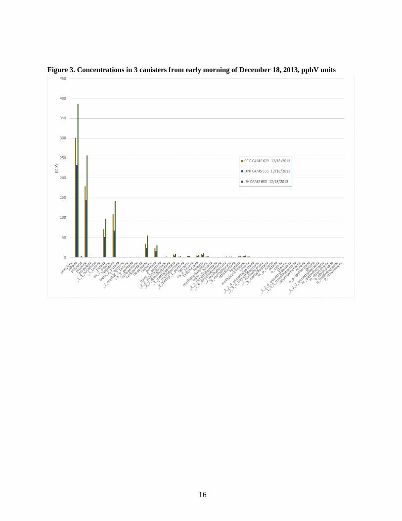
Figure 3. Concentrations in 3 canisters from early morning of December 18, 2013, ppbV units
16

Figure 4. Concentrations in 3 canisters from morning of February 13, 2014, ppbV units
Figure 5. Percent mass in various species, 3 canisters from early morning of December 18, 2013
17
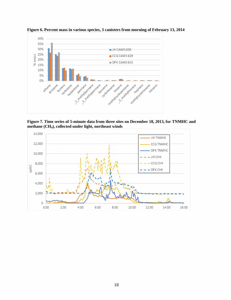
Figure 6. Percent mass in various species, 3 canisters from morning of February 13, 2014
Figure 7. Time series of 5-minute data from three sites on December 18, 2013, for TNMHC and methane (CH4), collected under light, northeast winds
18
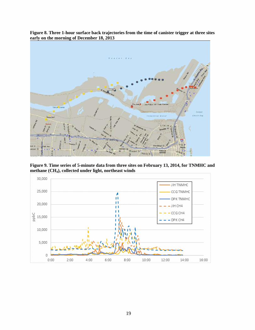
Figure 8. Three 1-hour surface back trajectories from the time of canister trigger at three sites early on the morning of December 18, 2013
Figure 9. Time series of 5-minute data from three sites on February 13, 2014, for TNMHC and methane (CH4), collected under light, northeast winds
19

Figure 10. Three 1-hour surface back trajectories from the time of canister trigger at three sites on the morning of February 13, 2014
The compositions of two additional canisters are shown in Figure 11, on page 21. These were the two canisters with the largest total sample masses: January 11, 2014, 8:40 CST at the J. I. Hailey CAMS 630 site measured 13,800 ppbC and March 15, 2014, 14:43 CST also at JI Hailey measured 13,400 ppbC. Although similar in total mass, the two canister samples were measured under very different conditions.
• The winds on the morning of January 11, 2014, were northwesterly averaging 5 mph over a two-hour period with TNMHC averaging 2,200 ppbC and methane measuring about 1,100 ppbC above background concentrations. The surface back-trajectory runs up to the White Point peninsula on the north side of Nueces Bay.
• The winds on the afternoon of March 15, 2014, were southerly back towards the docks and refinery areas averaging 12 mph over a 70 minute period over which 5-minute TNMHC values averaged 15,900 ppbC, with methane concentrations not significantly above background levels.
• Also, although similar in total mass, the two canister samples are very different in composition, as shown in Figure 11.
• The canister from January 11, 2014, 8:40 CST at JI Hailey contained a concentration of one hydrocarbon, m-ethyl toluene, at 23.4 ppbV, exceeding the TCEQ’s AMCV for odor of 18 ppbV. This was the only measurement made in FY 2014 above any TCEQ AMCV in a canister sample.
20

• Another difference between these two canister samples in Figure 11 is that the January 11 elevated concentration is suspected to have been the result of a very short-lived puff of polluted air, because the coincident, collocated TNMHC instrument did not measure concentrations as high as the canister. This is explained more below and on the following page. In contrast, the sample from March 15 did agree with the TNMHC instrument to within 11 percent.
No emission upset for a source in the general upwind area of JI Hailey is listed in the TCEQ upset database for either date. Figure 11. Concentrations in ppbV units in 2 canisters with the highest total mass in FY 2014: from 1/1/2014, 8:40 CST and from 3/15/2014, 14:43 CST, both at JI Hailey,
As just mentioned, one method of quality assurance is to compare the measurements made simultaneously by two different instruments or by two different analysis methods. Figure 12, on page 22, shows the results of comparing the sum of all individually measured hydrocarbon species concentrations for each canister analyzed by the UT Laboratory, with the simultaneously measured total nonmethane hydrocarbon concentration from the TNMHC analyzer quantified in real time. In Figure 12 for this comparison, 27 of 28 canisters are used, with one outlier excluded. As was mentioned in the preceding paragraph, the canister from January 11, 2014, 8:40 CST at the J. I. Hailey CAMS 630 site is an outlier, having measured 13,800 ppbC
21

compared to the simultaneous TNMHC instrument that measured an average of 1,943 ppbC. A close examination of the canister laboratory analysis data suggested the January 11 canister sample was legitimate, and the TNMHC instrument appeared to be operating correctly, having passed span checks before and after this canister trigger. A possible assignable cause of the observed difference is that a short puff of polluted air may have passed by the monitor during one of the short sampling time gaps in the TNMHC instrument. Overall, however, using 27 canister/TNMHC matches, the data fall along straight line with a near one-to-one match up. The best linear fit, shown in Figure 12, below, shows a slope of 0.85, which is less than 1.0, but with a positive y-intercept. When the regression is run with 0 for the y-intercept, the slope becomes 1.03, which is not statistically significantly different from 1.0. Figure 12. Comparison between the continuous TNMHC measurements with simultaneously collected total mass of known canister hydrocarbons, 27 of 28 canister samples, FY 2014
2. Summary of Total Nonmethane Hydrocarbon Monitoring at Seven Sites In this section, trends in total nonmethane hydrocarbon (TNMHC) concentrations at four UT CAMS sites – Port Grain C629, J. I. Hailey C630, FHR C632, and Dona Park C635 – are discussed. The data from each site, over each month from January 2005 through September 2014, are compared to assess seasonality and trends. As has been shown in past reports, each site measures its highest concentrations when the wind blows from the industrial source areas, including areas where natural gas extraction is occurring. Sites can measure elevated concentrations throughout the year, owing to exposure to industrial sources and natural gas extraction, as well as urban area emissions. Several meteorological factors affect the concentrations. In winter months, winds tend to be slower and the air does not mix as much as in
22

the summer, giving air pollutants more opportunities to accumulate. So all else being equal, one can expect higher concentrations for many pollutants in colder weather months. Wind direction also plays an important role. Because of concern about the frequency of elevated concentrations, the frequency (percent of measurements) of elevated TNMHC hourly events has been graphed in Figures 13 through 16, on pages 23 through 25. The frequency is determined by counting the number of hourly observations at or above 2000 ppbC and then dividing by the number of valid one hour observations per month (approximately 700). Each site’s data are graphed on different scales in the following figures. The FHR C632 site frequency values are graphed over the widest range, as that site had been affected by a particular source that has ceased operation, thus leading to a rapid decline in concentrations in late 2007. Two other sites also show a significant decline since 2005: Port Grain C629 and J. I. Hailey C630. The frequency may now be increasing at J.I. Hailey, with two months in FY 2014 above 1 percent. The Dona Park C635 site has shown dramatic changes from month to month, and realized an increase in frequency of elevated TNMHC concentrations in 2011. This is hypothesized to be related to natural gas extraction on the north side of Nueces Bay, but may also be related to nearby industrial activity and land use changes just to the north of the site. Figure 13. Frequency of hourly TNMHC >2000 ppbC at Port Grain C629, by month 2005- 2014
23

Figure 14. Frequency of hourly TNMHC >2000 ppbC at J. I. Hailey C630, by month 2005- 2014
Figure 15. Frequency of hourly TNMHC >2000 ppbC at Flint Hills Resources C632, by month 2005- 2014, by month 2005 - 2013
24

Figure 16. Frequency of hourly TNMHC >2000 ppbC at Dona Park C635, by month 2005- 2014
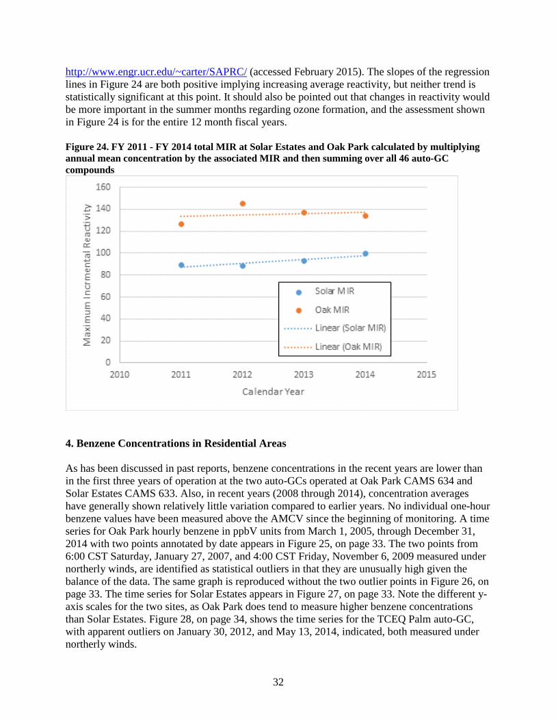
3. Auto-GC Data Summaries in Residential Areas In this section the results of semi-continuous sampling for 27 hydrocarbon species at the three Corpus Christi auto-GC sites – UT’s Solar Estates CAMS 633, UT’s Oak Park CAMS 634, and TCEQ’s Palm CAMS 83 – are presented. These three sites are located in residential areas. Solar Estates and Oak Park are generally downwind of industrial emissions under northerly winds. Palm, located near the TCEQ’s Hillcrest and Williams Park sites in Figure 1, on page 3, is generally downwind of industries under northerly and westerly winds. In examining the aggregated data, one observes similar patterns of hydrocarbon species at all three sites. Table 4, on page 26, lists the data completeness from the two project auto-GCs from January 2012 through December 2014. Data validation has been completed for all months for 2014. When data are missing, the reason is generally owing to quality assurance steps or maintenance procedures. The project regularly exceeds the minimum 75 percent data recovery goal.
25
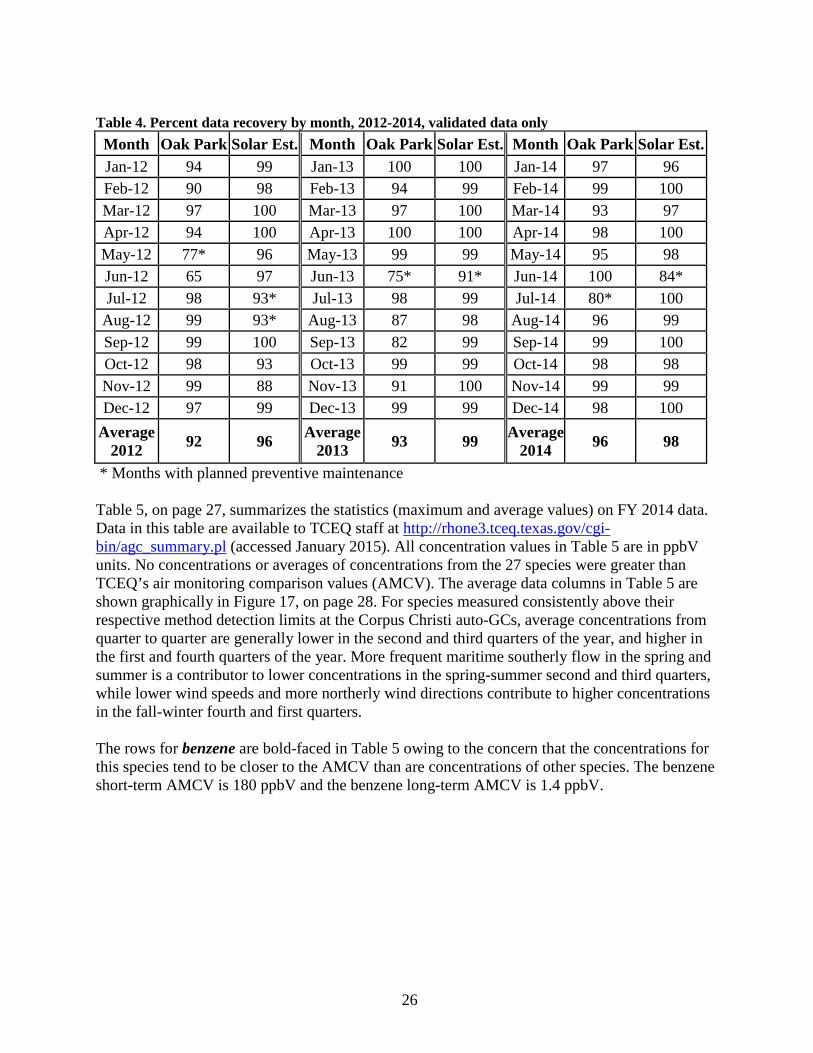
Table 4. Percent data recovery by month, 2012-2014, validated data only Month Oak Park Solar Est. Month Oak Park Solar Est. Month Oak Park Solar Est. Jan-12 94 99 Jan-13 100 100 Jan-14 97 96 Feb-12 90 98 Feb-13 94 99 Feb-14 99 100 Mar-12 97 100 Mar-13 97 100 Mar-14 93 97 Apr-12 94 100 Apr-13 100 100 Apr-14 98 100 May-12 77* 96 May-13 99 99 May-14 95 98 Jun-12 65 97 Jun-13 75* 91* Jun-14 100 84* Jul-12 98 93* Jul-13 98 99 Jul-14 80* 100
Aug-12 99 93* Aug-13 87 98 Aug-14 96 99 Sep-12 99 100 Sep-13 82 99 Sep-14 99 100 Oct-12 98 93 Oct-13 99 99 Oct-14 98 98 Nov-12 99 88 Nov-13 91 100 Nov-14 99 99 Dec-12 97 99 Dec-13 99 99 Dec-14 98 100
Average 2012 92 96 Average
2013 93 99 Average 2014 96 98
* Months with planned preventive maintenance Table 5, on page 27, summarizes the statistics (maximum and average values) on FY 2014 data. Data in this table are available to TCEQ staff at http://rhone3.tceq.texas.gov/cgi-bin/agc_summary.pl (accessed January 2015). All concentration values in Table 5 are in ppbV units. No concentrations or averages of concentrations from the 27 species were greater than TCEQ’s air monitoring comparison values (AMCV). The average data columns in Table 5 are shown graphically in Figure 17, on page 28. For species measured consistently above their respective method detection limits at the Corpus Christi auto-GCs, average concentrations from quarter to quarter are generally lower in the second and third quarters of the year, and higher in the first and fourth quarters of the year. More frequent maritime southerly flow in the spring and summer is a contributor to lower concentrations in the spring-summer second and third quarters, while lower wind speeds and more northerly wind directions contribute to higher concentrations in the fall-winter fourth and first quarters. The rows for benzene are bold-faced in Table 5 owing to the concern that the concentrations for this species tend to be closer to the AMCV than are concentrations of other species. The benzene short-term AMCV is 180 ppbV and the benzene long-term AMCV is 1.4 ppbV.
26

Table 5. Auto-GC statistics, FY 2014 Units ppbV Oak Park FY 2014 Solar Estates FY 2014 TCEQ Palm FY 2014
Species Peak 1hr
Peak 24hr
Average
Peak 1hr
Peak 24hr Mean Peak
1hr Peak 24hr
Average
Ethane 311.03
62.42
8.760 168.38
69.20
9.285 487.22
88.06
10.117 Ethylene 107.23
11.30
0.533 31.402 1.950 0.353 65.740 6.774 0.447
Propane 427.12
40.97
5.654 219.67
48.65
5.625 452.52
42.20
5.811 Propylene 35.659 3.926 0.237 39.008 2.242 0.187 26.905 2.930 0.200 Isobutane 79.593 15.86
1.853 38.791 10.91
1.620 210.87
23.60
2.222
n-Butane 78.247 19.46
2.893 50.516 19.17
2.581 223.06
25.93
3.485 t-2-Butene 1.412 0.310 0.057 4.091 0.232 0.027 22.622 1.459 0.062 1-Butene 0.964 0.167 0.039 3.014 0.343 0.023 24.260 1.617 0.095 c-2-Butene 1.710 0.297 0.041 4.399 0.227 0.014 14.701 0.949 0.045 Isopentane 51.701 8.631 1.579 78.582 6.214 1.162 83.948 11.01
1.677
n-Pentane 37.427 6.527 0.988 15.986 5.016 0.848 46.220 6.783 0.985 1,3-Butadiene 0.598 0.093 0.029 4.534 0.433 0.017 0.604 0.096 0.027 t-2-Pentene 4.013 0.436 0.047 5.539 0.261 0.011 6.790 0.856 0.069 1-Pentene 2.610 0.222 0.026 2.501 0.122 0.008 3.350 0.430 0.040 c-2-Pentene 2.144 0.209 0.023 2.694 0.126 0.004 3.544 0.433 0.035 n-Hexane 247.99
39.03
0.465 10.369 1.422 0.333 16.021 2.460 0.370
Benzene 9.203 2.055 0.286 4.093 0.636 0.142 59.412 4.844 0.265 Cyclohexane 9.129 2.253 0.199 3.034 0.582 0.140 7.583 1.190 0.130 Toluene 16.354 2.598 0.333 2.231 0.568 0.167 7.002 1.532 0.270 Ethyl Benzene 1.563 0.130 0.029 5.947 0.312 0.019 1.127 0.183 0.023 m&p -Xylene 6.318 0.481 0.104 25.184 2.085 0.146 5.286 0.919 0.110 o-Xylene 1.466 0.143 0.033 8.001 0.415 0.023 1.809 0.253 0.033 Isopropyl Benzene 1.395 0.276 0.020 1.394 0.118 0.007 1.032 0.204 0.006
1,3,5-Tri-methylbenzene 0.309 0.063 0.012 0.757 0.088 0.011 0.679 0.077 0.011
1,2,4-Tri-methylbenzene 0.545 0.138 0.038 0.750 0.125 0.020 0.952 0.136 0.030
n-Decane 0.647 0.125 0.023 2.259 0.174 0.031 1.770 0.139 0.019
1,2,3-Tri-methylbenzene 0.389 0.096 0.015 0.583 0.074 0.006 0.369 0.055 0.018
27

Figure 17. Mean ppbV for 27 species at project auto-GCs, FY 2014
As was reported in the recent quarterly reports and in the FY 2013 annual report, the annual and quarterly means concentrations from Solar Estates and Oak Park are higher over the last three years under northerly winds for ethane and propane and some other light alkane species than in the preceding three years. A preliminary hypothesis is that increased natural gas emissions is a possible assignable cause for the higher mean concentrations. Figure 18, on page 29, shows graphical summaries of the mean concentrations for the years FY 2005 through FY 2014 for Solar Estates for ethane and propane, two species found in natural gas, and two butane isomers, two pentane isomers, and n-hexane, which may be in natural gas and in other fuel products. Figure 19, on page 29, shows only the butane and pentane isomers and n-hexane to better show the change in these lower-concentration species over time, and Figure 20, on page 30, focuses on n-pentane and n-hexane at Solar Estates. The sequence of these three graphs is intended to show the weakening of the increasing trend in mean concentrations over FY 2011 to FY 2014 as the species become heavier1. There appears to be an upward trend for all seven species, though relatively weaker for n-hexane. Figures 21, 22, and 23, on pages 30 and 31, are similar graphs for the Oak Park site, for which the upward trend is most significant for ethane and n-butane, and very weak of n-pentane and n-hexane.
1 Ethane has two carbon atoms, propane has three, butanes have four, pentanes have five, and n-hexane has six.
28

Figure 18. Mean concentrations of ethane, propane, butane and pentane isomers, and hexane by FY at Solar Estates
Figure 19. Mean concentrations of butane and pentane isomers and hexane by year at Solar Estates
29

Figure 20. Mean concentrations of n-pentane and n-hexane by year at Solar Estates, intended to show the weakening of the upward trend with heavier species from 2011 to 2014
Figure 21. Mean concentrations of ethane, propane, butane and pentane isomers, and hexane by year at Oak Park
30

Figure 22. Mean concentrations of butane and pentane isomers and hexane by year at Oak Park
Figure 23. Mean concentrations of n-pentane and n-hexane by year at Oak Park, intended to show the weakening of the upward trend with heavier species from 2011 to 2014
Although the species with recent upward trends are not likely to approach or exceed TCEQ ACMVs, they nonetheless may have other effects on air quality such as increasing overall reactivity that influences ozone formation. Currently Corpus Christi has attainment status under the U.S. EPA’s NAAQS for ozone, but it is classified as a near-nonattainment area by the TCEQ. One method for assessing the effects of a chemical compound on ozone formation is to examine the maximum incremental reactivity (MIR) that relates the approximate increase in ozone associated with a unit increase of that chemical in a parcel of air, all else held equal. Figure 24, on page 32, shows the trend for the four years FY 2011 through FY 2014 for total MIR calculated by multiplying each annual mean concentration by the associated MIR and then summing over all 46 auto-GC compounds. More information on MIRs can be found at
31
http://www.engr.ucr.edu/~carter/SAPRC/ (accessed February 2015). The slopes of the regression lines in Figure 24 are both positive implying increasing average reactivity, but neither trend is statistically significant at this point. It should also be pointed out that changes in reactivity would be more important in the summer months regarding ozone formation, and the assessment shown in Figure 24 is for the entire 12 month fiscal years. Figure 24. FY 2011 - FY 2014 total MIR at Solar Estates and Oak Park calculated by multiplying annual mean concentration by the associated MIR and then summing over all 46 auto-GC compounds
4. Benzene Concentrations in Residential Areas As has been discussed in past reports, benzene concentrations in the recent years are lower than in the first three years of operation at the two auto-GCs operated at Oak Park CAMS 634 and Solar Estates CAMS 633. Also, in recent years (2008 through 2014), concentration averages have generally shown relatively little variation compared to earlier years. No individual one-hour benzene values have been measured above the AMCV since the beginning of monitoring. A time series for Oak Park hourly benzene in ppbV units from March 1, 2005, through December 31, 2014 with two points annotated by date appears in Figure 25, on page 33. The two points from 6:00 CST Saturday, January 27, 2007, and 4:00 CST Friday, November 6, 2009 measured under northerly winds, are identified as statistical outliers in that they are unusually high given the balance of the data. The same graph is reproduced without the two outlier points in Figure 26, on page 33. The time series for Solar Estates appears in Figure 27, on page 33. Note the different y-axis scales for the two sites, as Oak Park does tend to measure higher benzene concentrations than Solar Estates. Figure 28, on page 34, shows the time series for the TCEQ Palm auto-GC, with apparent outliers on January 30, 2012, and May 13, 2014, indicated, both measured under northerly winds.
32
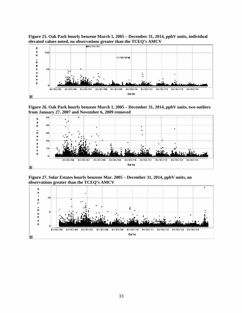
Figure 25. Oak Park hourly benzene March 1, 2005 – December 31, 2014, ppbV units, individual elevated values noted, no observations greater than the TCEQ’s AMCV
Figure 26. Oak Park hourly benzene March 1, 2005 – December 31, 2014, ppbV units, two outliers from January 27, 2007 and November 6, 2009 removed
Figure 27. Solar Estates hourly benzene Mar. 2005 – December 31, 2014, ppbV units, no observations greater than the TCEQ’s AMCV
33

Figure 28. TCEQ Palm hourly benzene June 1, 2010 – December 31, 2014, ppbV units, individual elevated value noted, no observations greater than the TCEQ’s AMCV
Table 6, on page 35, shows mean statistics for benzene at Oak Park and Solar Estates, by quarter 2005 – 2014, and at TCEQ Palm 2010 – 2014, ppbV units. The project now has more than nine years of complete data. Figure 29, on page 36, shows the quarterly means for the three sites since each started operation. This figure shows the strong seasonal effects, the early downward trend and subsequent flattening out in the trends at Oak Park and Solar Estates, and similarity between the Oak Park and TCEQ Palm benzene concentration means.
34

Table 6. Mean statistics for Benzene at Oak Park and Solar Estates, by quarter 2005 – 2014, Palm 2010 – 2014, ppbV units (1st quarter 2005 was March 2005 only)
Year Quarter Oak Park
Solar Estates
TCEQ Palm Year Quarter Oak
Park Solar Estates
TCEQ Palm
2005 1 0.32 0.37 2010 1 0.48 0.29 2005 2 0.20 0.25 2010 2 0.14 0.15 0.10 2005 3 0.30 0.27 2010 3 0.27 0.16 0.20 2005 4 1.30 0.41 2010 4 0.50 0.23 0.45 2006 1 0.81 0.34 2011 1 0.34 0.19 0.31 2006 2 0.31 0.18 2011 2 0.13 0.13 0.19 2006 3 0.52 0.32 2011 3 0.18 0.11 0.18 2006 4 1.14 0.58 2011 4 0.52 0.20 0.36 2007 1 1.04 0.43 2012 1 0.47 0.19 0.45 2007 2 0.32 0.23 2012 2 0.21 0.10 0.16 2007 3 0.42 0.25 2012 3 0.28 0.10 0.15 2007 4 0.68 0.37 2012 4 0.55 0.21 0.32 2008 1 0.46 0.26 2013 1 0.40 0.20 0.37 2008 2 0.14 0.13 2013 2 0.19 0.09 0.17 2008 3 0.23 0.17 2013 3 0.17 0.11 0.15 2008 4 0.63 0.31 2013 4 0.46 0.18 0.43 2009 1 0.43 0.25 2014 1 0.40 0.20 0.35 2009 2 0.17 0.14 2014 2 0.11 0.07 0.19 2009 3 0.28 0.12 2014 3 0.17 0.11 0.10 2009 4 0.81 0.28 2014 4 0.37 0.23 0.27
35
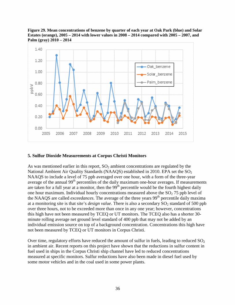
Figure 29. Mean concentrations of benzene by quarter of each year at Oak Park (blue) and Solar Estates (orange), 2005 – 2014 with lower values in 2008 – 2014 compared with 2005 – 2007, and Palm (gray) 2010 – 2014
5. Sulfur Dioxide Measurements at Corpus Christi Monitors As was mentioned earlier in this report, SO2 ambient concentrations are regulated by the National Ambient Air Quality Standards (NAAQS) established in 2010. EPA set the SO2 NAAQS to include a level of 75 ppb averaged over one hour, with a form of the three-year average of the annual 99th percentiles of the daily maximum one-hour averages. If measurements are taken for a full year at a monitor, then the 99th percentile would be the fourth highest daily one hour maximum. Individual hourly concentrations measured above the SO2 75 ppb level of the NAAQS are called exceedances. The average of the three years 99th percentile daily maxima at a monitoring site is that site’s design value. There is also a secondary SO2 standard of 500 ppb over three hours, not to be exceeded more than once in any one year; however, concentrations this high have not been measured by TCEQ or UT monitors. The TCEQ also has a shorter 30-minute rolling average net ground level standard of 400 ppb that may not be added by an individual emission source on top of a background concentration. Concentrations this high have not been measured by TCEQ or UT monitors in Corpus Christi. Over time, regulatory efforts have reduced the amount of sulfur in fuels, leading to reduced SO2 in ambient air. Recent reports on this project have shown that the reductions in sulfur content in fuel used in ships in the Corpus Christi ship channel have led to reduced concentrations measured at specific monitors. Sulfur reductions have also been made in diesel fuel used by some motor vehicles and in the coal used in some power plants.
36

In this section all monitors are looked at for their long term SO2 design value trends, with the recent fourth quarter of 2014 added in to complete calendar year 2014 and three year 2012-2014 periods. The overall conclusion is that there have been significant declines in the design values at all sites in Nueces County since monitoring for SO2 began at all sites, with one exception. That one exceptional site, Solar Estates CAMS 633, is hypothesized to have been affected by a chemical interferent. Table 7, below, shows a compilation of monitoring site SO2 design values going back to 2000 for TCEQ sites and 2006 for UT sites. The 2006 design value uses only two-years of data. What one observes from Table 7 is that the most recent design values are the lowest measured since each monitor began, the only exception being CAMS 633. Note that in the header row in Table 7 each site is identified with a “C” for CAMS and the site number. The TCEQ’s West site is CAMS 4, TCEQ’s Tuloso Middle School site is CAMS 21, and TCEQ’s Huisache site is CAMS 98. Table 7. Three-year SO2 design values for three TCEQ sites and six UT sites
3-yr period C4 C21 C98 C629 C630 C631 C632 C633 C635
1998-2000 34.5 28.3 66.6 1999-2001 33.6 26.2 67.0 2000-2002 29.7 20.4 77.9 2001-2003 31.7 18.8 81.3 2002-2004 35.5 14.3 73.4 2003-2005 37.0 14.0 60.5
2004-2006* 31.5 10.0 47.6 35.7 145.6 35.3 19.3 56.2 41.6 2005-2007 23.9 8.3 36.1 33.6 118.7 38.0 20.6 50.5 34.4 2006-2008 20.9 8.3 32.5 30.6 131.2 32.8 19.1 31.4 31.0 2007-2009 17.6 8.6 27.7 29.8 88.9 32.4 16.6 20.9 22.7 2008-2010 17.2 9.4 33.1 26.4 102.7 21.2 12.9 10.6 22.3 2009-2011 12.3 9.0 27.0 18.7 79.9 15.2 12.8 29.9 19.9 2010-2012 9.8 7.7 23.3 15.3 76.2 8.4 12.0 39.9 11.7 2011-2013 6.6 6.2 10.2 11.3 47.0 12.1 51.0 7.9 2012-2014 5.0 4.4 5.6 11.3 33.2 12.5 28.4 6.5
*only 2005 & 2006 for 2006 design value for six UT sites The data in Table 7 are graphed over time in several figures below using the end year of each 3-year period as the x-axis and design values on the y-axis. A line is provided where appropriate to indicate the level of the NAAQS. Figure 30, on page 38, shows the trend for all nine sites in Table 7. Figure 31, on page 38, shows the trend for the three TCEQ sites, which have operated since 1998. Figure 32, on page 39, shows the trend for four UT sites, which have operated since 2005 with the CAMS 631 site having ended in 2012. The two UT sites not shown in Figure 32 are shown separately in Figure 33, on page 39. In Figure 33, JIH CAMS 630 is shown with its steep decline in design values as sulfur content in fuels has dropped. Figure 33 also shows the fluctuating trend for Solar Estates CAMS 633, where a chemical interferent is no longer being detected since 2013, leading to a lower recent design value.
37

Figure 30. SO2 design values under current 2010 NAAQS in Nueces County
Figure 31. SO2 design values under current 2010 NAAQS at 3 TCEQ sites in Nueces County
38

Figure 32. SO2 design values under current 2010 NAAQS at four UT sites in Nueces County
Figure 33. SO2 design values under current 2010 NAAQS at two sites in Nueces County
Despite the decline in SO2 concentrations overall, there are still occasional exceedance events. On May 14, 2014 at 8 p.m. CST, a one-hour measurement at the FHR CAMS 632 site exceeded the 75 ppb level of the SO2 NAAQS. A time series of the hourly data for the FHR site and the nearby Solar Estates CAMS 633 site for May 14 and early May 15, 2014 appears in Figure 34, on page 40. The surface back trajectories from the two sites starting from the middle of the hour of peak concentration for each site (8:30 CST for FHR and 10:30 CST for Solar Estates) appear in Figure 35, on page 40, suggesting an industrial source to the north may have been the cause of the rise in concentrations at each site.
39

Figure 34. Time series of hourly SO2 data for FHR CAMS 632 and Solar Estates CAMS 633 site, May 14 and early May 15, 2014, red dashed line for the level of the NAAQS
Figure 35. Surface15-min. back trajectories from Solar Estates (on left) and FHR started from the middle of the hour with highest SO2 concentrations at each site on May 14, 2014
40
Conclusions from the FY 2014 Data In this annual report, several findings have been made:
• One exceedance of the EPA SO2 NAAQS level was measured in FY 2014 at a UT site. Dockside ship emissions that had affected the UT JIH CAMS 630 site appear to have diminished since June 2012, which is likely relatable to new federal rules on marine fuel. All Corpus Christi sites except one show a long term downward trend in SO2 NAAQS design values.
• FY 2014 concentrations at the auto-GCs remain well below the TCEQ’s AMCVs for all species tracked for this project. Trends in quarterly average benzene concentrations remain relatively flat in recent years. Mean concentrations for several hydrocarbon species, possibly associated with natural gas, have increased in the past three years.
• Periodic air pollution events continue to be measured on a routine basis. Further analyses will be provided upon request.
41

APPENDIX B
Web Site Statistics
42

Corpus Christi Air Monitoring and Surveillance Camera Installation and Operation Project Web Site Statistics
Calendar Year 2010 Calendar Year 2011 Calendar Year 2012 Calendar Year 2013 Calendar Year 2014Hits Views Visits Hits Views Visits Hits Views Visits Hits Views Visits Hits Views Visits
The University of Texas at Austin Corpus Christi Web Sites:Main Web Site (All Pages) 45,469 *** 115,823 *** 189,526 *** 336,946 *** 44,970 ***Trajectory Tool Web Site ("ceer_trajectory" directory) 39,388 9,292 29,154 9,285 26,083 9,179 22,321 8,815 42,245 11,513
SubTotal - UT Web Sites 84,857 0 9,292 144,977 0 9,285 215,609 0 9,179 359,267 0 8,815 87,215 0 11,513
TCEQ Web Sites:Monitoring Operations Corpus Christi AutoGC Page 1,324 2,015 1,077 1,051 27,113
SubTotal - TCEQ Web Sites 0 1,324 0 0 2,015 0 0 1,077 0 0 1,051 0 0 27,113 0
Total - Both Institutions 84,857 1,324 9,292 144,977 2,015 9,285 215,609 1,077 9,179 359,267 1,051 8,815 87,215 27,113 11,513
Denotes this count not collected.***
Definition of Terms:
Hit - A request for a file from the web server. Available only in log analysis. The number of hits received by a website is frequently cited to assert its popularity, but this number is extremely misleading and dramatically over-estimates popularity. A single web-page typically consists of multiple (often dozens) of discrete files, each of which is counted as a hit as the page is downloaded, so the number of hits is really an arbitrary number more reflective of the complexity of individual pages on the website than the website's actual popularity. The total number of visitors or page views provides a more realistic and accurate assessment of popularity.
According to UT-ITS the "Hit Count" from 2011 thru 2014 were being inflated by an erratic or misconfigured Google Search Application. The 2014 "Hits" were manually recounted and represent a more accurate assessment
Views are no longer available on UT's Urchin Weblog system since 2008.
TCEQ opened all 32 AGC site's to the public, since there are 2 Corpus Christi AGC sites, we use this formula ((Total Daily Views / 32) * 2) to estimate the Views for this report. TCEQ Information Resources reports the stats are inflated in 2014 because a new web server and a new webstats program were installed and the inflated numbers are due to something being counted differently.
Page View - A request for a file whose type is defined as a page in log analysis. An occurrence of the script being run in page tagging. In log analysis, a single page view may generate multiple hits as all the resources required to view the page (images, .js and .css files) are also requested from the web server.
Visit / Session - A series of requests from the same uniquely identified client with a set timeout. A visit is expected to contain multiple hits (in log analysis) and page views.
43

APPENDIX C
Financial Reports
44

ANNUAL PROGRESS REPORT TO THE U.S. DISTRICT COURT
FOR THE CORPUS CHRISTI NEIGHBORHOOD AIR TOXICS PROJECT
Financial Summary
As of September 30, 2014 Total Settlement Fund Allocation & Interest Earned $9,665,572.78
Stage 1 – Settlement Fund Allocation $4,586,014.92 Interest earned by the U.S. District Court $ 16,583.74 Additional interest earned by U.S. District Court $ 5,854.24 (Distributed by the Garden City Group in May 2010) Stage 1 Funds Total $4,608,452.90
Stage 1 Phase 1A - Modeling $2,277,564.00 Stage 1 Phase 1B – Monitoring Extension $2,330,888.90
Stage 2 Funds - Undistributed pending appeal $5,057,119.88 Based on the decision of the U.S. Court of Appeals for the 5th Circuit on June 27, 2011, UT Austin will not be receiving the Stage 2 funding at any point in the future. Less Stage 2 Funds ($5,057,119.88) Total Interest Earned at UT-Austin as of 9/30/2014 $ 391,349.93 Project Expenditures Stage 1, Phase 1A
First Year Paid Expenditures (3/3/2008 – 12/31/2008) $ 489,853.15 Second Year Paid Expenditures (1/1/2009 – 12/31/2009) $ 786,455.98 Third Year Paid Expenditures (1/1/2010 – 12/31/2010) $ 516,101.84 Fourth Year Paid Expenditures (1/1/2011 – 12/31/2011) $ 70,670.25 Total Project Expenditures (3/3/2008 – 12/31/2011) $1,863,081.22 Stage 1, Phase 1B First Year Paid Expenditures (1/1/2012 – 9/30/2012) $ 9,480.44 Second Year Paid Expenditures (10/1/2012 – 9/30/2013) $ 666,443.12 Third Year Paid Expenditures (10/1/2013 – 9/30/2014) $ 867,664.03 Total Project Expenditures (1/1/2012 – 9/30/14) $1,487,657.04
($3,350,738.26) Balance Remaining as of 9/30/14 $1,649,064.57
45

Exhibit A
CORPUS CHRISTI NEIGHBORHOOD AIR TOXICS PROJECT
Stage 1 Phase 1A – Modeling Funding Summary
Total Funding - Years 1 through 4 $2,277,564.00 Project Expenditures through 12/31/2011 $1,863,081.22
Stage1 Phase 1A Funds Remaining $ 414,482.78 Stage 1 Phase 1A Funds Transferred to Phase 1B ($ 414,482.78) Stage 1 Phase 1A Funds Final $ 0.00
Expenditure Summary for the Project Period
March 3, 2008 through December 31, 2011
Description
Budget Allocation Phase 1A
Years 1 - 4
Years 1- 3 paid
Expenditures
Year 4 paid
Expenditures Total
Expenditures Balance
Available Salaries and Wages $845,390.00 ($745,502.74) ($3,984.00) ($749,486.74) $95,903.26 Fringe Benefits $205,037.00 ($180,836.43) ($1,531.47) ($182,367.90) $22,669.10 CEER Admin Salaries $90,825.00 ($76,373.30) ($3,015.89) ($79,389.19) $11,435.81 Supplies $56,160.00 ($34,370.63) ($156.01) ($34,526.64) $21,633.36 Contingency $34,551.00 $0.00 $0.00 $0.00 $34,551.00 Consultants $25,000.00 $0.00 $0.00 $0.00 $25,000.00 Subcontract
Environ Corp. $400,000.00 ($319,985.42) ($40,980.38) ($360,965.80) $39,034.20 Texas A&M Univ. $195,763.00 ($172,305.78) ($11,784.64) ($184,090.42) $11,672.58
Holding $4,237.00 $0.00 $0.00 $0.00 $4,237.00 Modeling/Computer Services $59,000.00 $0.00 $0.00 $0.00 $59,000.00 Computation Center $1800.00 ($1800.00) $0.00 ($1,800.00) $0.00 Tuition $17,727.00 ($17,602.00) $0.00 ($17,602.00) $125.00 Travel $20,000.00 ($2,596.97) $0.00 ($2,596.97) $17,403.03
Equipment $25,000.00 ($7,245.00) $0.00 ($7,245.00) $17,755.00 Total Direct Costs $1,980,490.00 ($1,558,618.27) ($61,452.39) ($1,620,070.66) $360,419.34 Indirect Costs (15% TDC) $297,074.00 ($233,792.70) ($9,217.86) ($243,010.56) $54,063.44 Total $2,277,564.00 ($1,792,410.97) ($70,670.25) ($1,863,081.22) $414,482.78 In October 2011, all Phase 1A budget categories were rebudgeted to match total expenditures and leave a $0.00 balance. The remaining funds of $414, 482.78 were reallocated to Phase 1B.
46

Stage 1 Phase 1B – Air Monitoring Extension
Funding Allocation $2,330,888.90 Funds Transferred from Phase 1A $ 414,482.78 Total Funding Allocation $2,745,371.68 Interest Earned through 9/30/2014 $ 391,349.93 Total Funding Available $3,136,721.61 Project Expenditures through 09/30/2014 ($1,487,657.04) Funds Remaining $1,649,064.57
Expenditure Summary for the Project Period January 1, 2012 through September 30, 2014
Description
Year 1 & 2 1/1/12-9/30/13 Expenditures
Year 3 10/01/13-9/30/14
Expenditures
Total Expenditures as
of 9/30/14 Salaries and Wages ($49,252.93) ($120,918.56) ($170,171.49) Fringe Benefits ($15,069.99) ($33,589.17) ($48,659.16) CEER Admin Salaries ($13,387.58) ($25,985.86) ($39,373.44) Salary Holding $0.00 $0.00 $0.00 Quality Assurance $0.00 $0.00 $0.00 Cell Phone Allowance ($360.00) ($360.00) ($720.00) SEP Reserve $0.00 $0.00 $0.00 Contingency $0.00 $0.00 $0.00 Monthly M&O ($22,091.60) ($20,163.41) ($42,255.01) Equip. & Spare Parts ($24,323.29) ($3,208.81) ($27,532.10) Communications ($8,707.47) ($8,514.31) ($17,221.78) Electric ($23,086.69) ($21,070.77) ($44,157.46) Gases ($10,394.66) ($12,998.12) ($23,392.78) Consultant-Holding $0.00 $0.00 $0.00 Consultant Services $0.00 $0.00 $0.00
ORSAT ($173,964.06) ($187,509.75) ($361,473.81) TMSI ($169,927.45) ($241,227.32) ($411,154.77)
Analytical ($27,258.00) ($33,712.00) ($60,970.00) Travel ($1,300.62) ($1,532.38) ($2,833.00) Equipment $0.00 ($43,700.00) ($43,700.00) Total Direct Costs ($539,124.34) ($754,490.46) ($1,293,614.80) Indirect Costs (15% TDC) ($80,868.67) ($113,173.57) ($194,042.24)
Total ($619,993.01) ($867,664.03) ($1,487,657.04)
47

CORPUS CHRISTI AIR MONITORING AND SURVEILLANCE CAMERA PROJECT
University of Texas at Austin Annual Audit Report Results
The University’s Annual Reports and Audit Statements are made available for public review at the following website: http://www.sao.state.tx.us/reports/main/14-325.pdf Attached is a copy of The University of Texas at Austin’s Certification Statement for the Office of Management and Budget (OMB) Circular A-133 Audit conducted during the 2012/2013 fiscal year. The OMB Circular A-133 Audit for the 2012/2013 fiscal year is currently being conducted. The results of the 2011/2012 Audit will be made available at the above website. It is anticipated the audit results will be posted in late Spring 2015.
48

49

APPENDIX D
Supplemental Environmental Projects
SEP Project List
50

APPENDIX D
Supplemental Environmental Projects (SEP) awarded to The University of Texas at Austin
No. SEP (Name) Docket No. Period of
PerformanceAward
Amount
Interest Earned
as of 9/30/12
UT Account Number Project Description - Notes
1 CITGO Regfining and Chemicals Company, L.P.
2001-1469-AIR-E 7/2004-7/2006 $680,000.00 $19,978.03 26-7690-94 Task 1 - Extend the operation of the air monitoring network in Corpus Christi for an additional year.
$190,000.00 $7,956.39 26-7690-95 Task 2 - Development of the Trajectory Tool
2 Duke Energy Field Services
2003-1122-AIR-E 2/2005-8/2005 $5,187.00 $100.15 26-4254-75 Purchase additional canisters for the Corpus Christi monitoring sites.
3 El Paso Merchant Energy Petroleum Company
2001-1023-AIR-E 2/2006-6/2008 $46,004.00 $1,264.83 26-7693-36 Task 1 - Enchancement to the Automated Trajectory Tool.
$90,044.00 $5,790.85 26-7692-88 Task 2 - Additional Canister Analysis, Power Loss Hardware and Software and Wind Direction Filter.
4 Sherwin Aluminia 2004-1982-IR-E 10/2007-12/2009 $10,244.00 $557.00 26-7695-56 Used for canister analyses.
5 Texas Molecular Corpus Christi Services, Limited
D1-GV-07-001054 2/2009-9/2011 $67,900.00 $6,119.69 26-7697-82 Used for the repair and refurbishment of ageing equipment at the active Project sites. Items purchased include 8 computers and 3 multi-gas calibrators. Also, the Auto GC systems at Oak Park and Solar Estates were refurbished. * See note below.
6 Equistar Chemicals, LP D1-GV-06-002509 5/2012-5/2013 **See note below
$150,000.00 $114.56 26-7701-70 Funds will be used to extend and enhance the life of the Project Network. ** See note below
TOTAL $1,239,379.00 $41,881.50
* Originally the Texas Molecular and Equistar funds were to be used to purchase a FLIR ThermaCAM GasFindIR-HS (IR camera) and accessories, to train subcontractor personnel in use of camera,and to conduct video taping recording in the Corpus Christi refinery row area. When the Equistar funds were reduced (see note below) it was determined that the funding necessary for the camera was not available, and there were other ways the funds could be put to use to benefit the extension of the life of the network.
51

APPENDIX D
Supplemental Environmental Projects (SEP) awarded to The University of Texas at Austin
** A check in the amount of $400,000 was received by UT Austin 12/08/08 and was deposited in a holding account pending approval by the TCEQ of a UT Austin SEP Proposal. Subsequent to the March 31, 2009 Quarterly Report to the Court, the TCEQ notified UT Austin that Equistar Chemicals (a subsidiary of LyondellBasell Industries and US affiliate Loyondell Chemical Co.), filed for Chapter 11 bankruptcy on January 6, 2009 and that the $400,000 ordered to be paid by Equistar for this project might be subject to a collection effort in that proceeding on behalf of the creditors. As a consequence, the funding for the Equistar SEP award was placed on indefinite hold. Subsequently the Bankruptcy Trustee filed a lawsuit against UT to recover the $400,000 as a “preferential transfer” which can void transfers that take place within certain time limits of filing for bankruptcy.
The Texas Attorney General represented UT in that lawsuit. On February 7, 2011, UT was notified that the Assistant Attorney General handling the case, with the agreement of the TCEQ, succeeded in getting an agreed settlement under the terms of which UT paid $250,000 to the Bankruptcy Trustee and UT retained the remaining balance free and clear. On February 14, 2011, a payment in the amount of $250,000 was mailed to the Bankruptcy Trustee. Due to the reduction of the award amount and that a notice to proceed was never issued for the Equistar funds, UT contacted the TCEQ to determine the procedures UT should follow to move forward in utilizing the funds. On March 18, 2011, UT was asked to submit a new Third-Party Application to the SEP Program by June 1, 2011. This would allow UT to transition the Equistar funds to a new SEP Agreement, as the term of the older agreement has ended. UT submitted a new Third-Party Application to receive SEP funding on June 1, 2011. A contract for this new SEP Agreement was received on April 29, 2013 and was fully executed on July 10, 2013.On April 26, 2012, UT was contacted by Ms. Sharon Blue of the TCEQ regarding UT’s participation in the SEP program. Since the Third-Party Application is still under review, it was agreed that UT should issue a request to extend the prior SEP Agreement and move forward with utilizing the SEP funds. The extension request along with a project plan for utilizing the Equistar SEP funds was submitted to TCEQ in parallel with the March 31, 2012 Quarterly Report on May 7, 2012. On May 8, 2012, a No Cost Extension was granted until May 31, 2013.
52