Embed Size (px)
Citation preview
IT 13 073
Examensarbete 30 hpOktober 2013
Necessary Conditions for Constraint- based Register Allocation and Instruction Scheduling
Kim-Anh Tran
Institutionen för informationsteknologiDepartment of Information Technology

Teknisk- naturvetenskaplig fakultet UTH-enheten Besöksadress: Ångströmlaboratoriet Lägerhyddsvägen 1 Hus 4, Plan 0 Postadress: Box 536 751 21 Uppsala Telefon: 018 – 471 30 03 Telefax: 018 – 471 30 00 Hemsida: http://www.teknat.uu.se/student
Abstract
Necessary Conditions for Constraint-based RegisterAllocation and Instruction Scheduling
Kim-Anh Tran
Compilers translate code from a source language to a target language. Generatingoptimal code is thereby considered as infeasible due to the runtime overhead. Arather new approach is the implementation of a compiler by using ConstraintProgramming: in a constraint-based system, a problem is modeled by defining variablesand relations among these variables (that is, constraints) that have to be satisfied. Theapplication of a constraint-based compiler offers the potential of generating robustand optimal code. The performance of the system depends on the modeling choicesand constraints that are enforced. One way of refining a constraint model is theaddition of implied constraints. Implied constraints model logically redundant relationsamong variables, but provide distinct perspectives on the problem that might help tocut down the search effort. The actual impact of implied constraints is difficult toforesee, as they are tightly connected with the modeling choices made otherwise.This thesis investigates and evaluates a set of implied constraints that address registerallocation (decision where to store data) and instruction scheduling (decision when toexecute instructions) within an existing constraint-based compiler back-end. Itprovides insights into the impact on the code generation problem and discusses assetsand drawbacks of the set of introduced constraints.
Tryckt av: Reprocentralen ITCIT 13 073Examinator: Ivan ChristoffÄmnesgranskare: Christian SchulteHandledare: Mats Carlsson, Roberto Castañeda Lozano


ACKNOWLEDGMENTS
First, I would like to thank my supervisors Mats Carlsson and Roberto Cas-tañeda Lozano for the their continuous support, valuable advice and patience.Whenever I was stuck on a problem, Mats and Roberto took the time to answermy questions. It was a pleasure to work with you!
I would also like to thank my reviewer Christian Schulte, who encouraged meto participate at the SweConsNet 2013, which was a great experience. Through-out my thesis Christian was always very helpful and supportive.
Many thanks to my parents and my sister. I am grateful for everything yougave me and I hope that I can make it up to you one day!
Last but not least I want to thank Stephan Brandauer for the encouragement,the support and especially for making sure that I would not spend the wholeday in front of my laptop.
iv

CONTENTS
Acronyms 3
1 Introduction 5
1.1 Goal . . . . . . . . . . . . . . . . . . . . . . . . . . . . . . . . . . . 61.2 Thesis Outline . . . . . . . . . . . . . . . . . . . . . . . . . . . . . 6
2 Background 8
2.1 Compiler . . . . . . . . . . . . . . . . . . . . . . . . . . . . . . . . 82.2 Constraint Programming . . . . . . . . . . . . . . . . . . . . . . . 132.3 Constraint-Based Compiler Back-End . . . . . . . . . . . . . . . 18
3 Implied Constraints 30
3.1 Predecessor and Successor Constraints . . . . . . . . . . . . . . 303.2 Copy Activation Constraints . . . . . . . . . . . . . . . . . . . . . 343.3 Nogood Constraints . . . . . . . . . . . . . . . . . . . . . . . . . . 39
4 Implementation 48
4.1 Dependency Graph . . . . . . . . . . . . . . . . . . . . . . . . . . 484.2 Nogood Detection using MiniSat . . . . . . . . . . . . . . . . . . 52
5 Evaluation 53
5.1 Experimental Set Up . . . . . . . . . . . . . . . . . . . . . . . . . . 545.2 Experiment 1: Mips32 . . . . . . . . . . . . . . . . . . . . . . . . . 565.3 Experiment 2: Increased Duration . . . . . . . . . . . . . . . . . 645.4 Experiment 3: Increased Register Pressure . . . . . . . . . . . . . 685.5 Experiment 4: VLIW architecture . . . . . . . . . . . . . . . . . . 69
6 Discussion 74
7 Conclusion and Future Work 77
7.1 Results . . . . . . . . . . . . . . . . . . . . . . . . . . . . . . . . . . 777.2 Future Work . . . . . . . . . . . . . . . . . . . . . . . . . . . . . . . 78
A Figures 79
1
CONTENTS
B Constraint Model 84
B.1 Constraint Model . . . . . . . . . . . . . . . . . . . . . . . . . . . 84
Bibliography 88
2
ACRONYMS
ABI Application Binary Interface.
ALU Arithmetic Logic Unit.
BU Branching Unit.
CNF Conjunctive Normal Form.
COP Constraint Optimization Problem.
CP Constraint Programming.
CSP Constraint Satisfaction Problem.
ILP Integer Linear Programming.
IR Intermediate Representation.
LSSA Linear Static Single Assignment.
LSU Load/Store Unit.
SAT Boolean Satisfiability.
VLIW Very Long Instruction Word.
3

CH
AP
TE
R
1INTRODUCTION
High-level languages abstract from details of the underlying machine and thusenable programmers to implement portable, compact and expressive code. Inorder to run a program written in a high-level language, the source code needsto be translated into machine code that can be processed by the CPU.
The translation process is achieved by a compiler. A compiler is a programthat consists of two components: a front-end and a back-end. The front-endreads the input program and constructs an equivalent representation (Inter-mediate Representation (IR)) of the code that can be used by the back-end forgenerating the final machine code. There are three tasks that are associatedwith a compiler back-end: instruction selection (choose appropriate machineinstructions), instruction scheduling (create a schedule that specifies when toexecute which instruction) and register allocation (determine where to storedata).
Within the scope of this project, the focus lies on a compiler back-end thatis being developed using Constraint Programming (CP). CP is a methodologyfor solving combinatorial problems: a problem is expressed as a constraintmodel that consists of a set of variables and a set of constraints, which expressrelations among these variables that have to be true. A solution to a CP prob-lem is a complete variable-value assignment which satisfies all constraints.
Usually, instruction selection, instruction scheduling and register alloca-tion are solved in stages, i.e. one after another. This may result in suboptimalsolutions as the decisions in one part affects the decisions in the remainingparts. By formulating the code generation problem as one constraint modelthat has to be solved, instruction selection, instruction scheduling and regis-ter allocation are accomplished in consideration of each other. This may offer
5
CHAPTER 1. INTRODUCTION
possibilities for optimization as interdependencies between those tasks canbe exploited. On top of that, a constraint-based compiler has the potential ofgenerating optimal code. Finding an optimal solution is generally consideredas infeasible due to time concerns so that heuristics are applied instead.
The constraint model within this project incorporates both register alloca-tion and instruction scheduling. Instruction selection is not part of this com-piler and has thus to be accomplished before. In the scope of this master the-sis the aim is to investigate constraints that ideally optimize the solver’s perfor-mance by cutting down the search effort. If the constraints can detect conflict-ing assignments at an early stage within search, unnecessarily explored dead-ends can be avoided. These constraints are called implied constraints and donot change the set of solutions but add implied knowledge to the model thatcan be helpful during search. However, implied constraints have the poten-tial to improve, but also to worsen the performance of a solver; for instanceby adding too much computational overhead. Therefore, an evaluation of im-plied constraints is required.
1.1 Goal
The goal of the master thesis is the investigation, implementation and evalu-ation of static implied constraints addressing register allocation and instruc-tion scheduling in basic blocks. Basic blocks are maximal sequences of in-structions with only one entry point and one exit point. In order to providean insight into the impact of each constraint on the code generation problem,the thesis delivers:
• a set of implied constraints addressing register allocation and instruc-tion scheduling in basic blocks, and
• an evaluation of the impact of these on the search effort and thus asolver’s performance.
1.2 Thesis Outline
The remainder of this thesis is structured as follows. Chapter 2 covers back-ground knowledge and introduces related work. It describes the problem ofinstruction scheduling and register allocation, gives an overview on CP and
6
1.2. THESIS OUTLINE
presents the constraint model on hand. Chapter 3 introduces the set of im-plied constraints that are implemented and evaluated within this project. Theimplementation details are listed in Chapter 4 and the evaluation is presentedin Chapter 5. On the basis of the experiments, Chapter 6 discusses the impactof implied constraints on the code generation problem. Chapter 7 summa-rizes the results and gives a direction for future work. The bibliography con-tains information from the DBLP Computer Science Bibliography [24] whichis made available under the ODC Attribution License [6].
7
CH
AP
TE
R
2BACKGROUND
This chapter summarizes preliminaries that are relevant for the following chap-ters. It is divided into three parts: Section 2.1 describes the base problem of in-struction scheduling and register allocation. Section 2.2 gives an overview onconstraint programming. Finally, Section 2.3 introduces the base constraintmodel with its variables and constraints.
2.1 Compiler
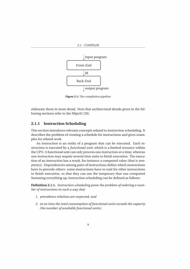
A compiler translates a program from a source language into a target language.The translation process is called compilation and consists of two separatestages: program analysis and program synthesis [1]. The first stage of programanalysis is performed by a compiler front-end. The front-end checks the in-put program against syntactic and semantic correctness and only if no errorswere found, an equivalent but more compact representation of the input pro-gram is created. The created IR serves as an input to the compiler back-endduring the second stage. The compiler back-end first maps instructions ofthe IR to appropriate machine instructions (instruction selection) that can beprocessed by the CPU. Then it generates a schedule for instructions that deter-mines the order in which instructions are executed (instruction scheduling).Finally, it selects the location where computed values are stored (register allo-cation). Figure 2.1 shows the compiler components and their respective inputand output values. In the context of this thesis, the focus lies on the compilerback-end and its two tasks of instruction scheduling and register allocation.The following sections will introduce terms associated with both tasks and
8
2.1. COMPILER
Front-End
Back-End
input program
IR
output program
Figure 2.1: The compilation pipeline
elaborate them in more detail. Note that architectural details given in the fol-lowing sections refer to the Mips32 [20].
2.1.1 Instruction Scheduling
This section introduces relevant concepts related to instruction scheduling. Itdescribes the problem of creating a schedule for instructions and gives exam-ples for related work.
An instruction is an entity of a program that can be executed. Each in-struction is executed by a functional unit, which is a limited resource withinthe CPU. A functional unit can only process one instruction at a time, whereasone instruction may require several time units to finish execution. The execu-tion of an instruction has a result, for instance a computed value (that is tem-
porary). Dependencies among pairs of instructions define which instructionshave to precede others: some instructions have to wait for other instructionsto finish execution, so that they can use the temporary that was computed.Summing everything up, instruction scheduling can be defined as follows:
Definition 2.1.1. Instruction scheduling poses the problem of ordering a num-
ber of instructions in such a way that
1. precedence relations are respected, and
2. at no time the total consumption of functional units exceeds the capacity
(the number of available functional units).
9
CHAPTER 2. BACKGROUND
b0:. . .
b1:. . .
b2:. . .
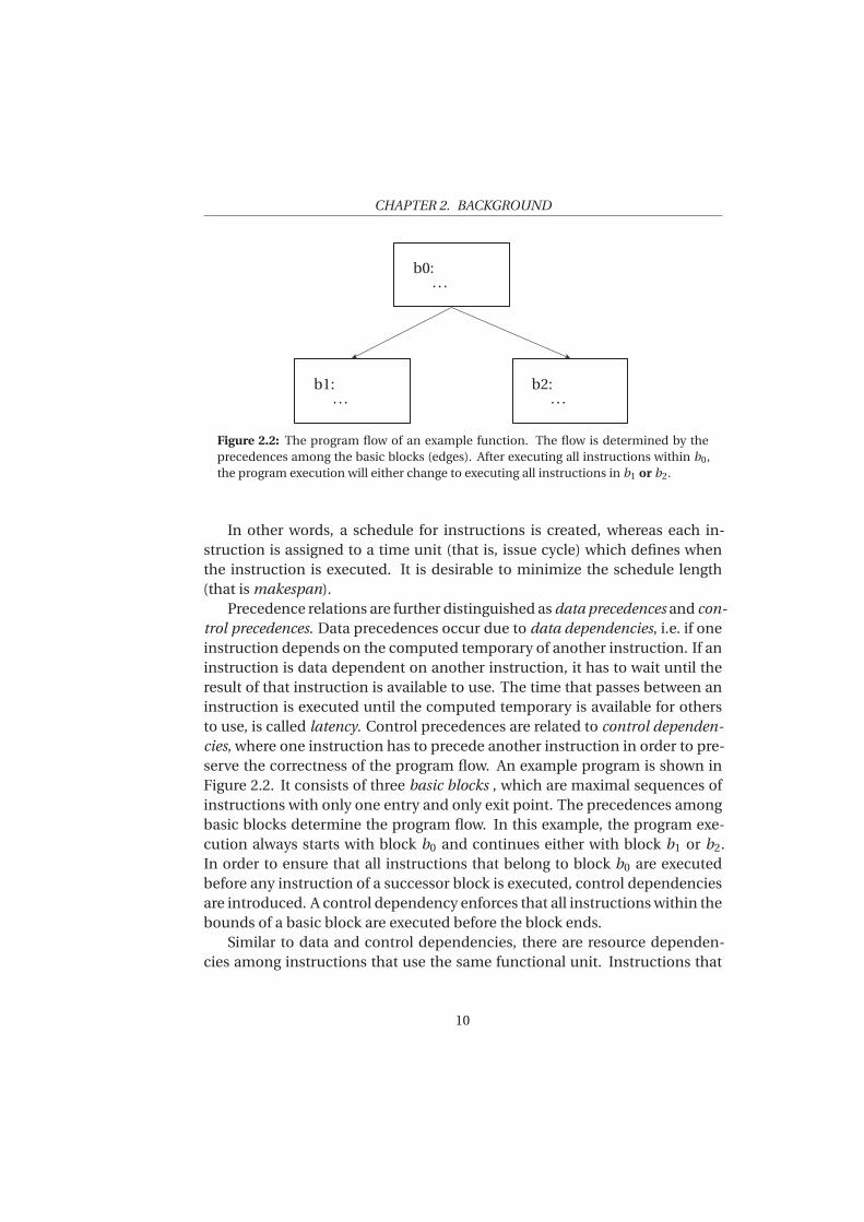
Figure 2.2: The program flow of an example function. The flow is determined by theprecedences among the basic blocks (edges). After executing all instructions within b0,the program execution will either change to executing all instructions in b1 or b2.
In other words, a schedule for instructions is created, whereas each in-struction is assigned to a time unit (that is, issue cycle) which defines whenthe instruction is executed. It is desirable to minimize the schedule length(that is makespan).
Precedence relations are further distinguished as data precedences and con-
trol precedences. Data precedences occur due to data dependencies, i.e. if oneinstruction depends on the computed temporary of another instruction. If aninstruction is data dependent on another instruction, it has to wait until theresult of that instruction is available to use. The time that passes between aninstruction is executed until the computed temporary is available for othersto use, is called latency. Control precedences are related to control dependen-
cies, where one instruction has to precede another instruction in order to pre-serve the correctness of the program flow. An example program is shown inFigure 2.2. It consists of three basic blocks , which are maximal sequences ofinstructions with only one entry and only exit point. The precedences amongbasic blocks determine the program flow. In this example, the program exe-cution always starts with block b0 and continues either with block b1 or b2.In order to ensure that all instructions that belong to block b0 are executedbefore any instruction of a successor block is executed, control dependenciesare introduced. A control dependency enforces that all instructions within thebounds of a basic block are executed before the block ends.
Similar to data and control dependencies, there are resource dependen-cies among instructions that use the same functional unit. Instructions that
10
2.1. COMPILER
share the same functional unit are dependent on each other. For instance, ifone instruction needs to consume a functional unit that is currently occupiedby another instruction, it has to wait until the functional unit becomes avail-able, which is the case if the currently executed instruction finishes. The timespan, in which an instruction uses a functional unit for execution, is therebycalled duration.
Optimal instruction scheduling on basic blocks has been approached be-fore as an Integer Linear Programming (ILP) [27, 2]. The instruction schedulerby Wilken et al. [27] optimally solves basic blocks of a size of up to 1000 instruc-tions. Their solution is based on a simplified integer program that is obtainedby graph transformations on the dependency graph. A dependency graphis a directed acyclic graph that represents instructions and their dependen-cies: instructions are nodes and dependencies are edges. The solution pro-posed by Bednarski et al. [2] solves instruction selection, instruction schedul-ing and register allocation for basic blocks. Their approach optimally solvesbasic blocks up to a size of 22 instructions. Instruction scheduling has alsobeen modeled as a CP problem ([9, 18]). Ertl et al. [9] use constraint logic pro-gramming and consistency techniques to optimally solve basic blocks up to asize of 50 instructions [17]. Malik et al. [18] present an optimal scheduler thatsolves blocks of a size up to 2600 instructions while remaining in a reasonabletime limit.
The constraint model that is used in the current compiler back-end tosolve instruction scheduling will be covered in Section 2.3.3.1. From here on,functional units are generally addressed as resources that are consumed by in-structions.
2.1.2 Register Allocation
This section introduces terms associated with register allocation. It definesthe problem and lists related work.
An architecture can have multiple, addressable storage banks to whichtemporaries that are computed are stored to. The thesis distinguishes be-tween two distinct storage banks: registers and main memory. Processor reg-isters are part of the CPU. Data that resides in registers can be retrieved morequickly than data that is stored in memory. For this reason it is desirable tostore as many temporaries as possible in registers. Distinct temporaries canbe assigned to the same register as long as their live ranges do not overlap.
11
CHAPTER 2. BACKGROUND
The live range of a temporary is defined as follows: the live range of a tempo-rary starts with the temporary definition (that is the execution of its definerinstruction) and ends with the last instruction that uses it. To be more precise,the live range ends with the last instruction that uses it and might be executed.The program flow is not statically defined (conditional jumps between basicblocks) and thus it is not known for every instruction whether it will be exe-cuted or not. In case a temporary is used by an instruction that might be exe-cuted at a later stage, the temporary has to remain live. Putting this together,register allocation can be defined as follows:
Definition 2.1.2. Register allocation poses the problem of defining which tem-
poraries are kept in registers in such a way that:
1. no two distinct temporaries that are live at the same time are assigned to
the same register.
Some temporaries are already pre-assigned to registers. Pre-assigned tem-poraries have to reside in a specific register due to architectural constraints.All temporaries that are not pre-assigned, can either be stored in a register orin memory. Even if it is desirable to store temporaries in registers, some tem-poraries have to be stored in memory instead as the number of registers islimited. This is known as spilling.
The traditional approach of solving register allocation is graph coloring.With k being the number of available registers, register allocation can be re-duced to the question, whether an interference graph is k-colorable. In otherwords, does a coloring with k colors exist, so that two connected nodes alwayshave distinct colors. An interference graph illustrates which temporaries can-not reside in the same register. The nodes in an interference graph are tem-poraries and the edges represent interferences. If two nodes are connected,they cannot reside in the same register. Register allocation and spilling usinggraph coloring is first implemented by Chaitin [4].
Goodwin et al. [12] present an ILP model for register allocation that sig-nificantly reduces the spill code overhead (instructions that copy a temporaryfrom and to memory) compared to the traditional graph coloring approach.However, their solution suffers from high compilation time when generatingoptimal solutions. Bednarski et al. [2] solve both register allocation and in-struction scheduling using ILP.
Section 2.3.3.2 covers the modeling choices for solving register allocationusing CP.
12
2.2. CONSTRAINT PROGRAMMING
2.2 Constraint Programming
This section first introduces the concept of Constraint Programming. It givesan overview on how problems can be modeled using CP and how solutionscan be found. It thereby focuses on the two fundamental aspects of CP, namelypropagation and search. After a basic understanding of constraints, it explainsthe meaning of implied constraints, which are the focus within the context ofthis thesis.
CP is a methodology that is used for solving combinatorial problems. InCP, a problem is formulated as a model that consists of variables, their poten-tial values and constraints. If we take the context of a compiler back-end as anexample, a possible variable set would be the issue cycle ci of each instructioni that has to be scheduled. An example set of potential values for their issuecycles is {0, . . . ,n} ,n ∈N. Some instructions might have to be scheduled afterother instructions due to dependencies. Such dependencies can be formu-lated as constraints. Given two instructions i and j , assume that i has to bescheduled before j . The corresponding constraint would then be expressedas follows: ci < c j . In other words, the issue cycle of i has to be smaller thanthe issue cycle of instruction j . A solution to a constraint problem is foundby search. The solution search generates a search tree branching on potentialvariable values that are picked due to a chosen heuristic. At each node, the re-sulting domains are systematically reduced, using propagation. Propagationremoves values that are guaranteed to result in a failure, as these values, ifassigned to the corresponding variable, conflict with the defined constraints.Values conflict with a constraint, if assigning that value to the correspondingvariable can never satisfy the relation that a constraint defines. In the result-ing tree, each leaf is either a solution (assignments to variables satisfy all con-straints) or a failed node (assignments conflict with at least one constraint).
Based on this intuition, some definitions related with constraint program-ming follow. The notation in this section is partly taken from [21] and [18].
Definition 2.2.1. A Constraint Satisfaction Problem (CSP) is described by a
triple ⟨V ,D,C⟩: A set of variables V , a set of variable domains D and the set
of constraints C . A variable vi ∈ V = v1, . . . , vn has potential values defined in
the domain Di ∈ D. Each constraint ci ∈ C defines a relation between a set
of variables vars(c) ⊂ V . A solution to a CSP is a complete assignment of one
value to each variable, so that all constraints are satisfied. A variable is said to
be assigned, if its domain only contains one value.
13
CHAPTER 2. BACKGROUND
Definition 2.2.2. A Constraint Optimization Problem (COP)⟨
V ,D,C , f⟩
is a
CSP that defines an additional objective function f . Likewise, a solution to a
COP is a complete assignment of one value to each variable, so that all con-
straints are satisfied. Each solution is mapped to a cost value by the objective
function f and the goal is to find a solution that minimizes or maximizes that
value.
The code generation problem within this project is a COP.
2.2.1 Propagation and Consistency
Propagation is the process of manipulating variable domains. Each constraintis associated with one propagator. A propagator removes (that is prunes) val-ues from variable domains that are known not be part of a solution: givena constraint c, a propagator prunes a value x in the domain of a variablev, v ∈ vars(c), if assigning x to v will never satisfy the corresponding constraint.On the contrary, if for the assignment of v = x assignments to the remainingvariables vi ∈ vars(c) \ {v} exist, so that a solution to c is formed, the assign-ment v = x is said to be supported. In this case, the assignments to the vari-ables vi is the support for v = x. A propagator for a constraint is said to be atfixpoint, if running that propagator again will not have an effect on the currentvariable domains. In case a propagator will never change a variable domainagain (as the constraint will always be satisfied for the current assignments),the propagator is entailed. There are different types of consistencies that canbe enforced on a constraint. The consistency determines the strength of prop-agation, i.e. how many values are pruned. The prevalent types of consisten-cies that can be enforced on a constraints are Value Consistency, Bounds
Consistency and Domain Consistency. Strong propagation is more effectivethough time consuming. The appropriate consistency to choose is thereforedepending on the problem on hand. In the following, the three consistenciesare defined.
This definition of value consistency is taken from [3].
Definition 2.2.3. Partition vars(c) into avars(c), the assigned variables, and
uvars(c), the unassigned variables.
A constraint c is value consistent, iff for every v ∈ uvars(c) and x in the domain
of v, avars(c)∪ {v = x} can be extended to a solution of c, where uvars(c) \ {v}may take any values, irrespective of their domains.
14
2.2. CONSTRAINT PROGRAMMING
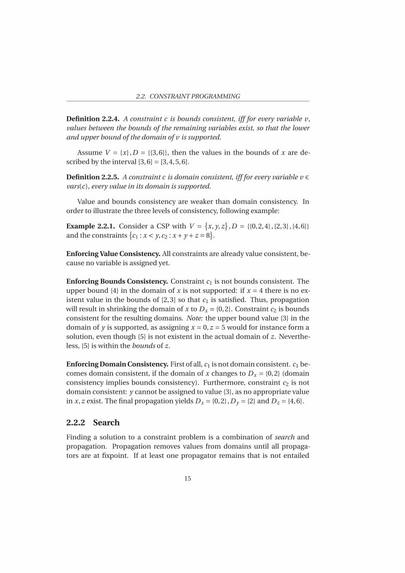
Definition 2.2.4. A constraint c is bounds consistent, iff for every variable v,
values between the bounds of the remaining variables exist, so that the lower
and upper bound of the domain of v is supported.
Assume V = {x} ,D = {{3,6}}, then the values in the bounds of x are de-scribed by the interval [3,6] = [3,4,5,6].
Definition 2.2.5. A constraint c is domain consistent, iff for every variable v ∈
vars(c), every value in its domain is supported.
Value and bounds consistency are weaker than domain consistency. Inorder to illustrate the three levels of consistency, following example:
Example 2.2.1. Consider a CSP with V ={
x, y, z}
,D = {{0,2,4} , {2,3} , {4,6}}and the constraints
{
c1 : x < y,c2 : x + y + z = 8}
.
Enforcing Value Consistency. All constraints are already value consistent, be-cause no variable is assigned yet.
Enforcing Bounds Consistency. Constraint c1 is not bounds consistent. Theupper bound {4} in the domain of x is not supported: if x = 4 there is no ex-istent value in the bounds of [2,3] so that c1 is satisfied. Thus, propagationwill result in shrinking the domain of x to Dx = {0,2}. Constraint c2 is boundsconsistent for the resulting domains. Note: the upper bound value {3} in thedomain of y is supported, as assigning x = 0, z = 5 would for instance form asolution, even though {5} is not existent in the actual domain of z. Neverthe-less, {5} is within the bounds of z.
Enforcing Domain Consistency. First of all, c1 is not domain consistent. c1 be-comes domain consistent, if the domain of x changes to Dx = {0,2} (domainconsistency implies bounds consistency). Furthermore, constraint c2 is notdomain consistent: y cannot be assigned to value {3}, as no appropriate valuein x, z exist. The final propagation yields Dx = {0,2} ,D y = {2} and Dz = {4,6}.
2.2.2 Search
Finding a solution to a constraint problem is a combination of search andpropagation. Propagation removes values from domains until all propaga-tors are at fixpoint. If at least one propagator remains that is not entailed
15
CHAPTER 2. BACKGROUND
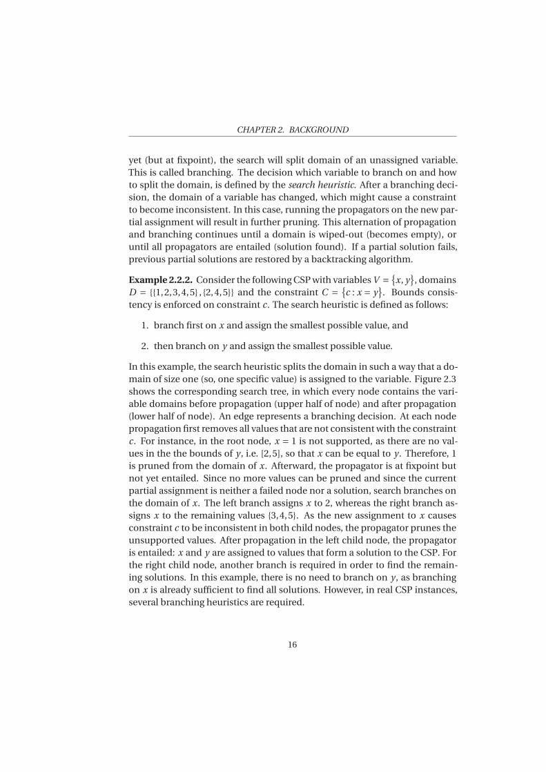
yet (but at fixpoint), the search will split domain of an unassigned variable.This is called branching. The decision which variable to branch on and howto split the domain, is defined by the search heuristic. After a branching deci-sion, the domain of a variable has changed, which might cause a constraintto become inconsistent. In this case, running the propagators on the new par-tial assignment will result in further pruning. This alternation of propagationand branching continues until a domain is wiped-out (becomes empty), oruntil all propagators are entailed (solution found). If a partial solution fails,previous partial solutions are restored by a backtracking algorithm.
Example 2.2.2. Consider the following CSP with variables V ={
x, y}
, domainsD = {{1,2,3,4,5} , {2,4,5}} and the constraint C =
{
c : x = y}
. Bounds consis-tency is enforced on constraint c. The search heuristic is defined as follows:
1. branch first on x and assign the smallest possible value, and
2. then branch on y and assign the smallest possible value.
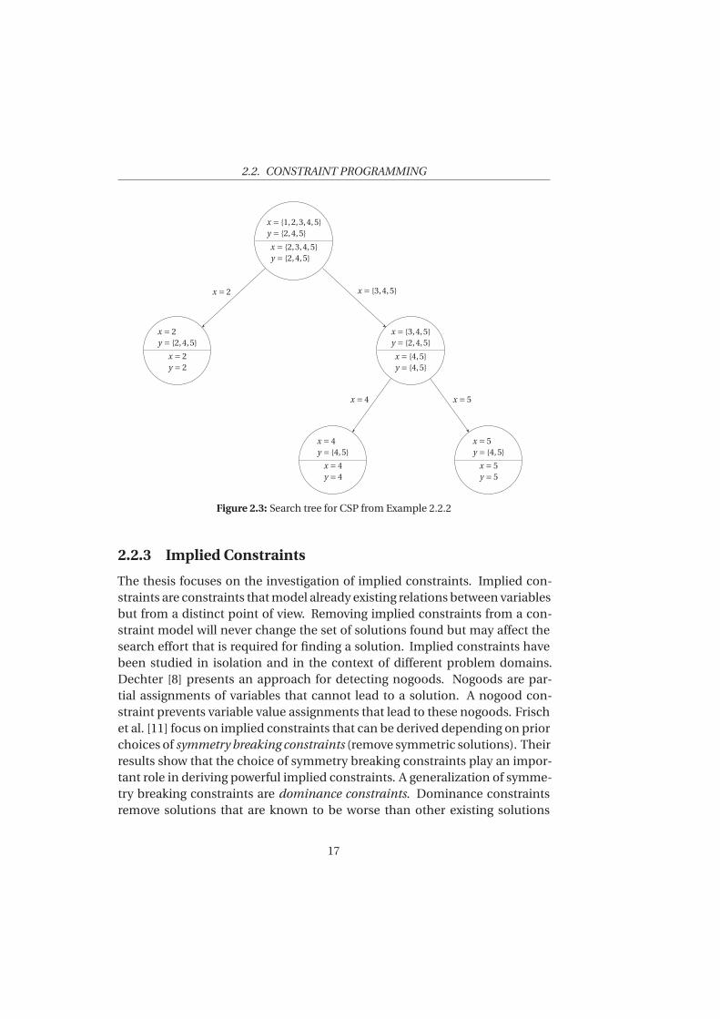
In this example, the search heuristic splits the domain in such a way that a do-main of size one (so, one specific value) is assigned to the variable. Figure 2.3shows the corresponding search tree, in which every node contains the vari-able domains before propagation (upper half of node) and after propagation(lower half of node). An edge represents a branching decision. At each nodepropagation first removes all values that are not consistent with the constraintc. For instance, in the root node, x = 1 is not supported, as there are no val-ues in the the bounds of y , i.e. [2,5], so that x can be equal to y . Therefore, 1is pruned from the domain of x. Afterward, the propagator is at fixpoint butnot yet entailed. Since no more values can be pruned and since the currentpartial assignment is neither a failed node nor a solution, search branches onthe domain of x. The left branch assigns x to 2, whereas the right branch as-signs x to the remaining values {3,4,5}. As the new assignment to x causesconstraint c to be inconsistent in both child nodes, the propagator prunes theunsupported values. After propagation in the left child node, the propagatoris entailed: x and y are assigned to values that form a solution to the CSP. Forthe right child node, another branch is required in order to find the remain-ing solutions. In this example, there is no need to branch on y , as branchingon x is already sufficient to find all solutions. However, in real CSP instances,several branching heuristics are required.
16
2.2. CONSTRAINT PROGRAMMING
x = {1,2,3,4,5}y = {2,4,5}
x = {2,3,4,5}y = {2,4,5}
x = {3,4,5}y = {2,4,5}
x = {4,5}y = {4,5}
x = 5y = {4,5}
x = 5y = 5
x = 4y = {4,5}
x = 4y = 4
x = 4 x = 5
x = 2y = {2,4,5}
x = 2y = 2
x = 2 x = {3,4,5}
Figure 2.3: Search tree for CSP from Example 2.2.2
2.2.3 Implied Constraints
The thesis focuses on the investigation of implied constraints. Implied con-straints are constraints that model already existing relations between variablesbut from a distinct point of view. Removing implied constraints from a con-straint model will never change the set of solutions found but may affect thesearch effort that is required for finding a solution. Implied constraints havebeen studied in isolation and in the context of different problem domains.Dechter [8] presents an approach for detecting nogoods. Nogoods are par-tial assignments of variables that cannot lead to a solution. A nogood con-straint prevents variable value assignments that lead to these nogoods. Frischet al. [11] focus on implied constraints that can be derived depending on priorchoices of symmetry breaking constraints (remove symmetric solutions). Theirresults show that the choice of symmetry breaking constraints play an impor-tant role in deriving powerful implied constraints. A generalization of symme-try breaking constraints are dominance constraints. Dominance constraintsremove solutions that are known to be worse than other existing solutions
17
CHAPTER 2. BACKGROUND
front-end instruction selector s2ls
extender modeler solver synthesizer
.c .s
.ext.ls .json .out.json .out.asm
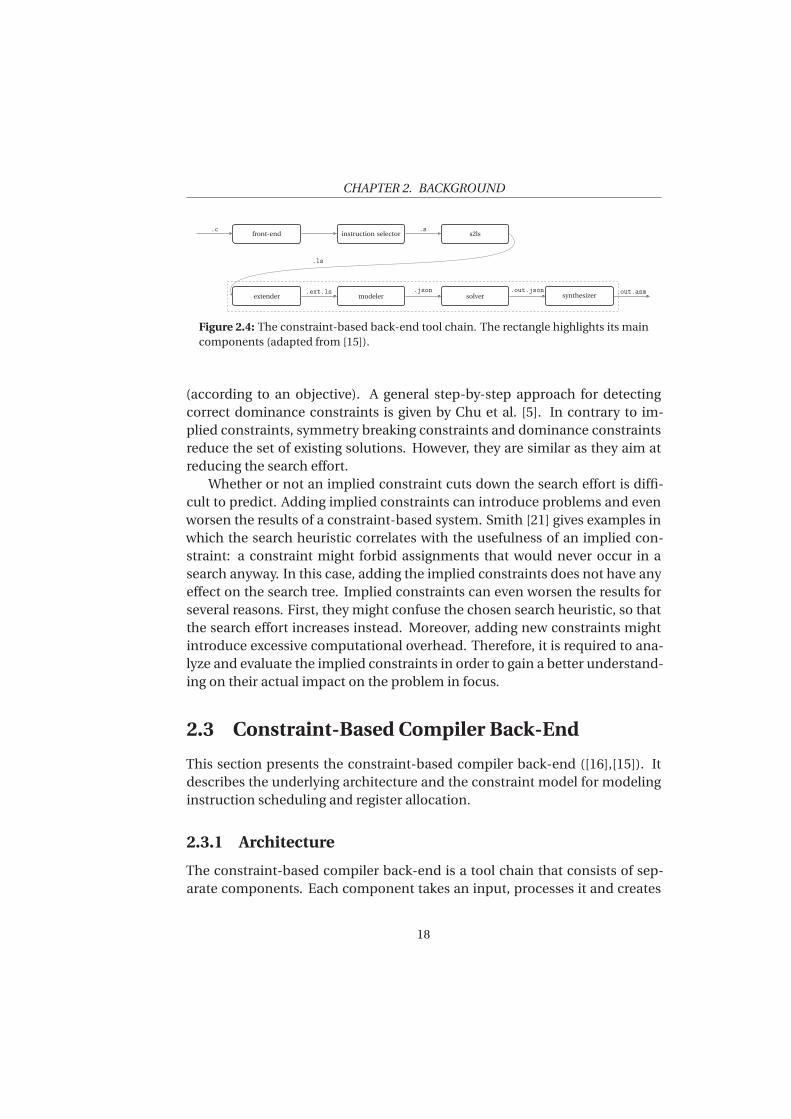
.ls
Figure 2.4: The constraint-based back-end tool chain. The rectangle highlights its maincomponents (adapted from [15]).
(according to an objective). A general step-by-step approach for detectingcorrect dominance constraints is given by Chu et al. [5]. In contrary to im-plied constraints, symmetry breaking constraints and dominance constraintsreduce the set of existing solutions. However, they are similar as they aim atreducing the search effort.
Whether or not an implied constraint cuts down the search effort is diffi-cult to predict. Adding implied constraints can introduce problems and evenworsen the results of a constraint-based system. Smith [21] gives examples inwhich the search heuristic correlates with the usefulness of an implied con-straint: a constraint might forbid assignments that would never occur in asearch anyway. In this case, adding the implied constraints does not have anyeffect on the search tree. Implied constraints can even worsen the results forseveral reasons. First, they might confuse the chosen search heuristic, so thatthe search effort increases instead. Moreover, adding new constraints mightintroduce excessive computational overhead. Therefore, it is required to ana-lyze and evaluate the implied constraints in order to gain a better understand-ing on their actual impact on the problem in focus.
2.3 Constraint-Based Compiler Back-End
This section presents the constraint-based compiler back-end ([16],[15]). Itdescribes the underlying architecture and the constraint model for modelinginstruction scheduling and register allocation.
2.3.1 Architecture
The constraint-based compiler back-end is a tool chain that consists of sep-arate components. Each component takes an input, processes it and creates
18
2.3. CONSTRAINT-BASED COMPILER BACK-END
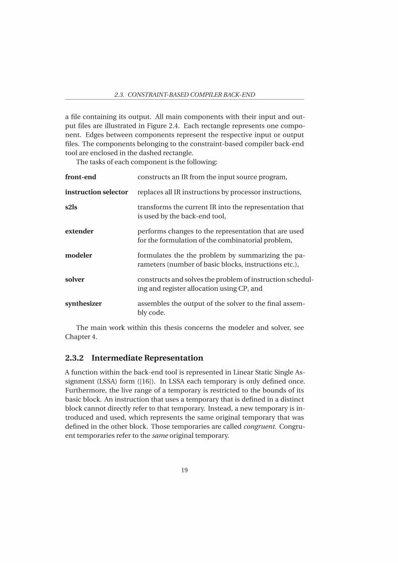
a file containing its output. All main components with their input and out-put files are illustrated in Figure 2.4. Each rectangle represents one compo-nent. Edges between components represent the respective input or outputfiles. The components belonging to the constraint-based compiler back-endtool are enclosed in the dashed rectangle.
The tasks of each component is the following:
front-end constructs an IR from the input source program,
instruction selector replaces all IR instructions by processor instructions,
s2ls transforms the current IR into the representation thatis used by the back-end tool,
extender performs changes to the representation that are usedfor the formulation of the combinatorial problem,
modeler formulates the the problem by summarizing the pa-rameters (number of basic blocks, instructions etc.),
solver constructs and solves the problem of instruction schedul-ing and register allocation using CP, and
synthesizer assembles the output of the solver to the final assem-bly code.
The main work within this thesis concerns the modeler and solver, seeChapter 4.
2.3.2 Intermediate Representation
A function within the back-end tool is represented in Linear Static Single As-signment (LSSA) form ([16]). In LSSA each temporary is only defined once.Furthermore, the live range of a temporary is restricted to the bounds of itsbasic block. An instruction that uses a temporary that is defined in a distinctblock cannot directly refer to that temporary. Instead, a new temporary is in-troduced and used, which represents the same original temporary that wasdefined in the other block. Those temporaries are called congruent. Congru-ent temporaries refer to the same original temporary.
19
CHAPTER 2. BACKGROUND
The representation is extended by the extender to include two major changesthat are relevant for the formulation of register allocation. First, the exten-der adds optional copy instructions to the already existing set of instructions.Copy instructions are instructions that copy the value of one temporary to an-other temporary. They are optional, as it is not decided yet, whether or notto actually use and schedule them (see Section 2.3.3.2). Temporaries that arecopies of each other are copy related.
Second, up until here, instructions were said to use temporaries and com-pute temporaries. This change is a generalization of that idea: instructionsuse operands and define operands that can in turn be implemented by a tem-porary. Operands can be implemented by a range of temporaries. By the in-troduction of copy instructions, the operand used by an instruction can beimplemented either by the original temporary or by any copy related one. Incase that a copy instruction is inactive, its operands are not used and thusimplemented by a dummy temporary, the null temporary.
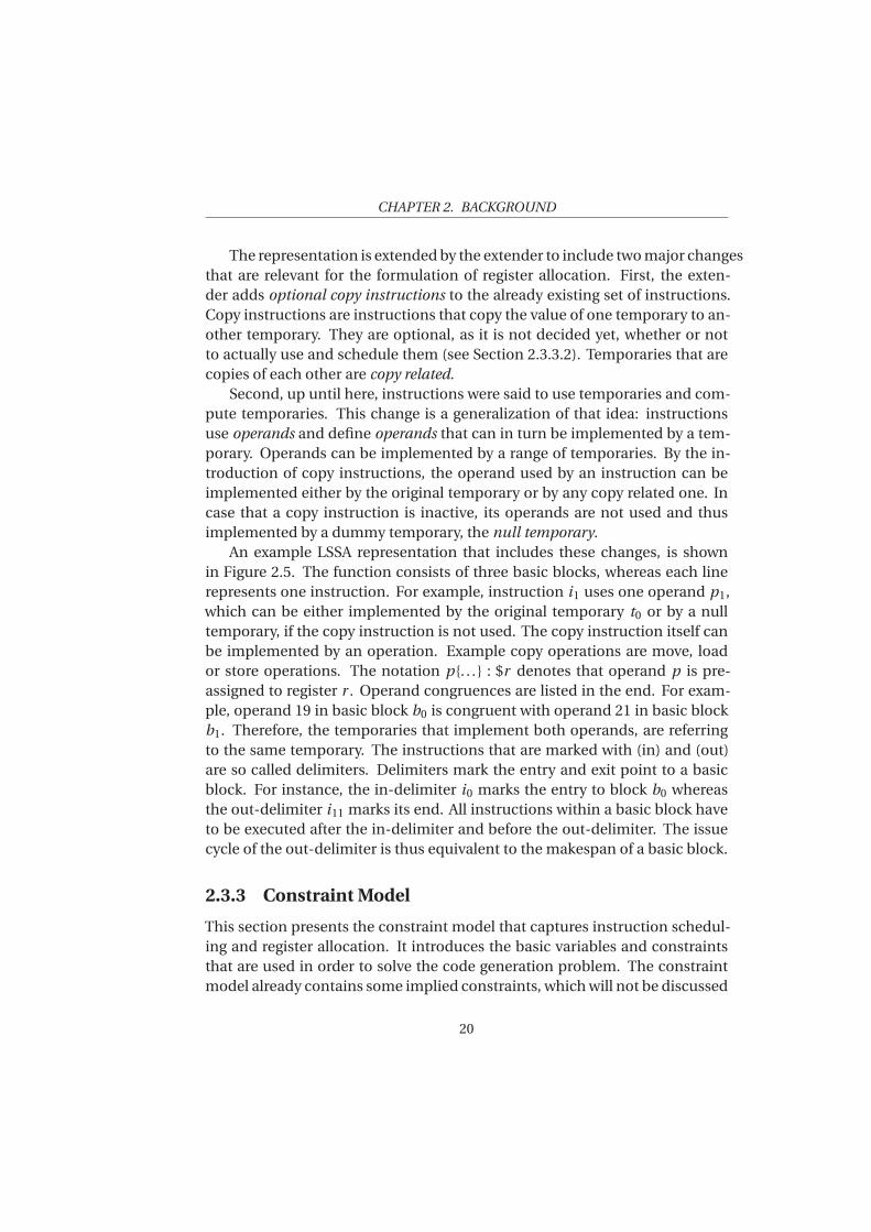
An example LSSA representation that includes these changes, is shownin Figure 2.5. The function consists of three basic blocks, whereas each linerepresents one instruction. For example, instruction i1 uses one operand p1,which can be either implemented by the original temporary t0 or by a nulltemporary, if the copy instruction is not used. The copy instruction itself canbe implemented by an operation. Example copy operations are move, loador store operations. The notation p{. . . } : $r denotes that operand p is pre-assigned to register r . Operand congruences are listed in the end. For exam-ple, operand 19 in basic block b0 is congruent with operand 21 in basic blockb1. Therefore, the temporaries that implement both operands, are referringto the same temporary. The instructions that are marked with (in) and (out)are so called delimiters. Delimiters mark the entry and exit point to a basicblock. For instance, the in-delimiter i0 marks the entry to block b0 whereasthe out-delimiter i11 marks its end. All instructions within a basic block haveto be executed after the in-delimiter and before the out-delimiter. The issuecycle of the out-delimiter is thus equivalent to the makespan of a basic block.
2.3.3 Constraint Model
This section presents the constraint model that captures instruction schedul-ing and register allocation. It introduces the basic variables and constraintsthat are used in order to solve the code generation problem. The constraintmodel already contains some implied constraints, which will not be discussed
20
2.3. CONSTRAINT-BASED COMPILER BACK-END
b0:
i0: [p0{t0}:$4] <- (in) []
i1: [p2{-, t1}] <- {null, move, sw} [p1{-, t0}]
i2: [p3{t2}] <- addiuz [1]
i3: [p5{-, t3}] <- {null, move, sw} [p4{-, t2}]
i4: [p7{-, t4}] <- {null, move, lw} [p6{-, t0, t1}]
i5: [p9{t5}] <- slti [p8{t0, t1, t4, t8},1]
i6: [p11{-, t6}] <- {null, move, sw} [p10{-, t5}]
i7: [p13{-, t7}] <- {null, move, lw} [p12{-, t5, t6}]
i8: [p15{-, t8}] <- {null, move, lw} [p14{-, t0, t1}]
i9: [p17{-, t9}] <- {null, move, lw} [p16{-, t2, t3}]
i10: [] <- bnez [p18{t5, t6, t7},b2]
i11: [] <- (out) [p19{t0, t1, t4, t8},p20{t2, t3, t9}]
b1:
i12: [p21{t10},p22{t11}] <- (in) []
i13: [p24{-, t12}] <- {null, move, sw} [p23{-, t10}]
i14: [p26{-, t13}] <- {null, move, sw} [p25{-, t11}]
i15: [p28{-, t14}] <- {null, move, lw} [p27{-, t10, t12}]
i16: [p30{-, t15}] <- {null, move, lw} [p29{-, t11, t13}]
i17: [p33{t16}] <- mul [p31{t10, t12, t14, t18},p32{t11, t13, t15}]
i18: [p35{-, t17}] <- {null, move, sw} [p34{-, t16}]
i19: [p37{-, t18}] <- {null, move, lw} [p36{-, t10, t12}]
i20: [p39{t19}] <- addiu [p38{t10, t12, t14, t18},-1]
i21: [p41{-, t20}] <- {null, move, sw} [p40{-, t19}]
i22: [p43{-, t21}] <- {null, move, lw} [p42{-, t19, t20}]
i23: [p45{-, t22}] <- {null, move, lw} [p44{-, t16, t17}]
i24: [p47{-, t23}] <- {null, move, lw} [p46{-, t19, t20}]
i25: [] <- bgtz [p48{t19, t20, t21, t23},b1]
i26: [] <- (out) [p49{t16, t17, t22},p50{t19, t20, t21, t23}]
b2:
i27: [p51{t24}] <- (in) []
i28: [p53{-, t25}] <- {null, move, sw} [p52{-, t24}]
i29: [p55{-, t26}] <- {null, move, lw} [p54{-, t24, t25}]
i30: [] <- jra []
i31: [] <- (out) [p56{t24, t25, t26}:$2]
congruences:
p19 = p21, p20 = p22, p20 = p51, p49 = p22, p49 = p51, p50 = p21
prologue:
(...)
epilogue:
(...)
Figure 2.5: Factorial function in LSSA representation. Reprinted from [15].
21
CHAPTER 2. BACKGROUND
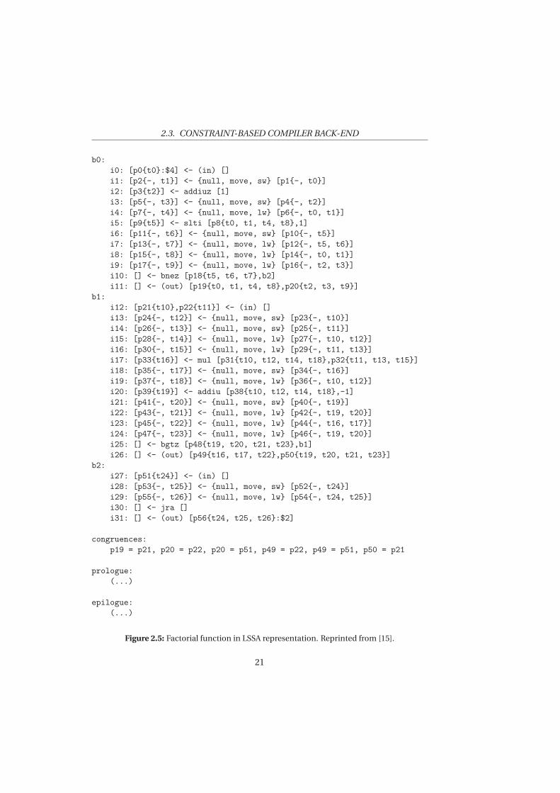
B , I ,P,T sets of blocks, instructions, operands and temporariesins(b) set of instructions of block b
tmp(b) set of temporaries defined and used within block b
operands(i ) set of operands defined and used by instruction i
definer(t ) instruction that defines temporary t
p ≡ q whether operands p and q are congruentt⊲r whether temporary t is pre-assigned to register r
dist(i , j ,op) min. issue distance of instrs. i and j when i is imple-mented by operation op
use(p) whether p is a use operand
temps(p) set of temporaries that can implement operand p
cdep set of control dependencies (i , j ) defined on two instruc-tions i and j
freq(b) estimation of the execution frequency of block b
Table 2.1: Program parameters. Taken and adapted from [15].
further. For the complete model, see the paper by Castañeda et al. [16] and theimplementation notes [15]. The model described in the paper differs in somedetails with the model used in the context of this thesis. Therefore, Appendix Bshows the base model version on which this thesis is based on.
In the following, relevant program and processor parameters are intro-duced, which are used for formulating the constraints of the model for instruc-tion scheduling (Section 2.3.3.1) and register allocation (Section 2.3.3.2).
The presented parameters and constraints are simplified for the sake ofclarity. Furthermore the thesis only introduces a subset of the model and itsparameters.
22
2.3. CONSTRAINT-BASED COMPILER BACK-END
O,R sets of processor operations and resources
operations(i ) set of operations that can implement instruction i
lat(op) latency of operation op
cap(r ) capacity of processor resource r
con(op,r ) consumption of processor resource r by operation op
dur(op,r ) duration of usage of processor resource r by operationop
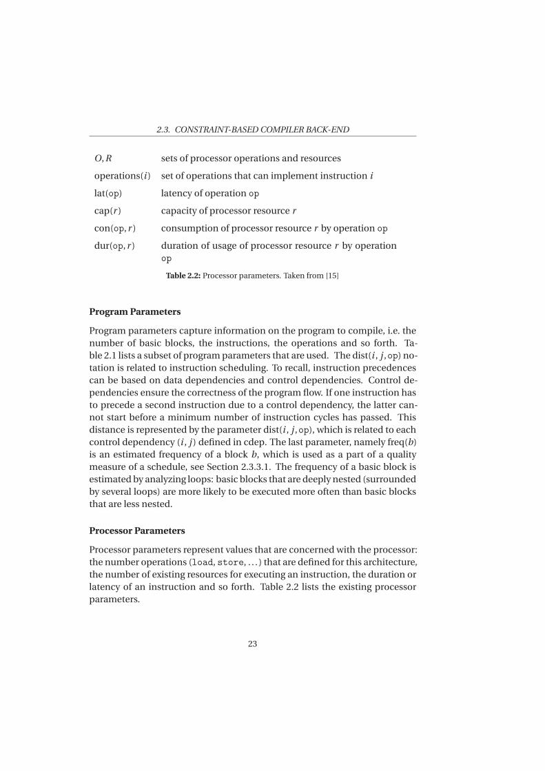
Table 2.2: Processor parameters. Taken from [15]
Program Parameters
Program parameters capture information on the program to compile, i.e. thenumber of basic blocks, the instructions, the operations and so forth. Ta-ble 2.1 lists a subset of program parameters that are used. The dist(i , j ,op) no-tation is related to instruction scheduling. To recall, instruction precedencescan be based on data dependencies and control dependencies. Control de-pendencies ensure the correctness of the program flow. If one instruction hasto precede a second instruction due to a control dependency, the latter can-not start before a minimum number of instruction cycles has passed. Thisdistance is represented by the parameter dist(i , j ,op), which is related to eachcontrol dependency (i , j ) defined in cdep. The last parameter, namely freq(b)is an estimated frequency of a block b, which is used as a part of a qualitymeasure of a schedule, see Section 2.3.3.1. The frequency of a basic block isestimated by analyzing loops: basic blocks that are deeply nested (surroundedby several loops) are more likely to be executed more often than basic blocksthat are less nested.
Processor Parameters
Processor parameters represent values that are concerned with the processor:the number operations (load, store, . . . ) that are defined for this architecture,the number of existing resources for executing an instruction, the duration orlatency of an instruction and so forth. Table 2.2 lists the existing processorparameters.
23
CHAPTER 2. BACKGROUND
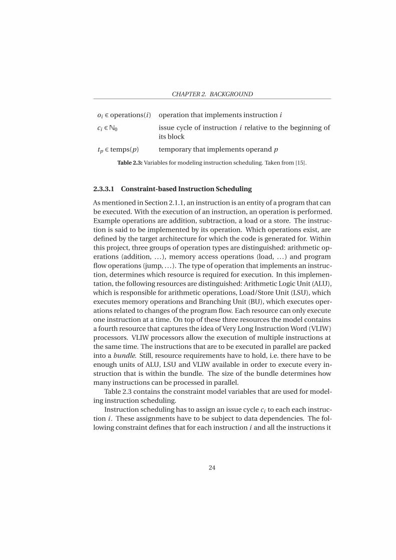
oi ∈ operations(i ) operation that implements instruction i
ci ∈N0 issue cycle of instruction i relative to the beginning ofits block
tp ∈ temps(p) temporary that implements operand p
Table 2.3: Variables for modeling instruction scheduling. Taken from [15].
2.3.3.1 Constraint-based Instruction Scheduling
As mentioned in Section 2.1.1, an instruction is an entity of a program that canbe executed. With the execution of an instruction, an operation is performed.Example operations are addition, subtraction, a load or a store. The instruc-tion is said to be implemented by its operation. Which operations exist, aredefined by the target architecture for which the code is generated for. Withinthis project, three groups of operation types are distinguished: arithmetic op-erations (addition, . . . ), memory access operations (load, . . . ) and programflow operations (jump, . . . ). The type of operation that implements an instruc-tion, determines which resource is required for execution. In this implemen-tation, the following resources are distinguished: Arithmetic Logic Unit (ALU),which is responsible for arithmetic operations, Load/Store Unit (LSU), whichexecutes memory operations and Branching Unit (BU), which executes oper-ations related to changes of the program flow. Each resource can only executeone instruction at a time. On top of these three resources the model containsa fourth resource that captures the idea of Very Long Instruction Word (VLIW)processors. VLIW processors allow the execution of multiple instructions atthe same time. The instructions that are to be executed in parallel are packedinto a bundle. Still, resource requirements have to hold, i.e. there have to beenough units of ALU, LSU and VLIW available in order to execute every in-struction that is within the bundle. The size of the bundle determines howmany instructions can be processed in parallel.
Table 2.3 contains the constraint model variables that are used for model-ing instruction scheduling.
Instruction scheduling has to assign an issue cycle ci to each each instruc-tion i . These assignments have to be subject to data dependencies. The fol-lowing constraint defines that for each instruction i and all the instructions it
24
2.3. CONSTRAINT-BASED COMPILER BACK-END
depends on, i can never start before the used value is defined:
tp = t =⇒ ci ≥ cdefiner(t ) + lat(odefiner(t ))
∀t ∈ temps(p), ∀p ∈ operands(i ) : use(p), ∀i ∈ I(3.1)
So, for all of the used operands operands(i ), if the operand is implemented bya temporary tp = t , then the instruction i can start earliest after the definer oft ,definer(t ), is issued and the latency has passed. The latency is dependenton the operation that implements the definer of t .
A similar constraint is added for control dependencies:
c j ≥ ci +dist(i , j ,oi ) ∀(
i , j)
∈ cdep (3.2)
For all control dependencies between two instructions i and j where i hasto precede j , instruction j cannot be executed until instruction i has beenexecuted and until a minimum number of additional cycles (the distance)has passed. One example set of control dependencies is related to the out-delimiter: all instructions that belong to a basic block have to be executedbefore the respective out-delimiter.
Finally, instruction scheduling is subject to resource constraints. At noissue cycle, the number of required resources may exceed the number of ex-isting resources (the capacity cap(r )). If an instruction i uses a resource r ,its consumption of r , i.e. con(oi ,r ) is greater than zero. For each availableresource r ∈ R, each basic block b ∈ B , the following constraint is added:
cumulative({⟨ci ,dur(oi ,r ),con(oi ,r )⟩:i∈ins(b)} ,cap(r )) ∀b∈B ,∀r∈R (3.3)
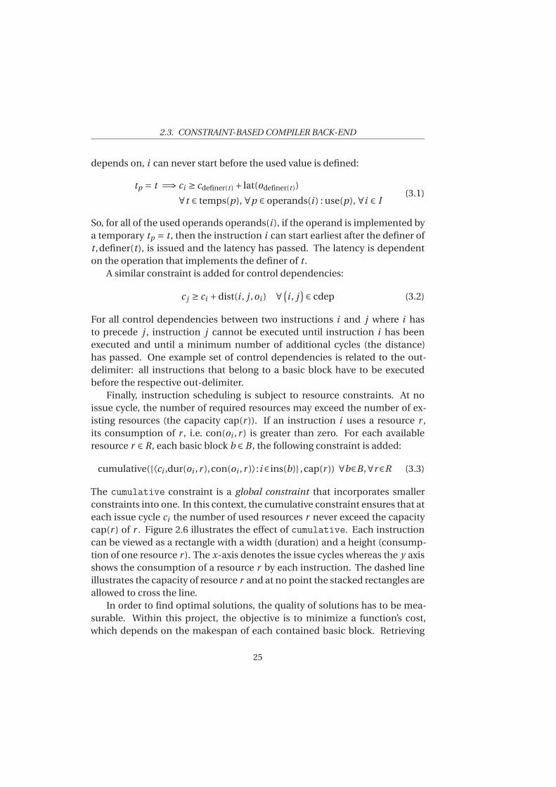
The cumulative constraint is a global constraint that incorporates smallerconstraints into one. In this context, the cumulative constraint ensures that ateach issue cycle ci the number of used resources r never exceed the capacitycap(r ) of r . Figure 2.6 illustrates the effect of cumulative. Each instructioncan be viewed as a rectangle with a width (duration) and a height (consump-tion of one resource r ). The x-axis denotes the issue cycles whereas the y axisshows the consumption of a resource r by each instruction. The dashed lineillustrates the capacity of resource r and at no point the stacked rectangles areallowed to cross the line.
In order to find optimal solutions, the quality of solutions has to be mea-surable. Within this project, the objective is to minimize a function’s cost,which depends on the makespan of each contained basic block. Retrieving
25
CHAPTER 2. BACKGROUND
Issue cycle
Resource consumption
Capacity
Figure 2.6: Illustration of a cumulative constraint and its effect for a given resource r .Each instruction is represented as a rectangle that has a duration (width) and a resourceconsumption (height). The x-axis corresponds to the issue cycle and the y-axis to theconsumption of resource r . At no point, the stacked rectangles (total consumption) areallowed to exceed the capacity of resource r (dashed line)
the makespan of a basic block is trivial, as no jumps occur within a block: themakespan of a basic block is equivalent to the issue cycle of its last to be ex-ecuted instruction. The cost of a function is the weighted sum of each basicblock’s makespan:
minimize∑
b∈B
freq(b)× maxi∈ins(b)
ci (3.4)
The frequencies freq(b) allow a more accurate computation of the cost. How-ever, only estimated frequencies are used, as the frequency of a basic blockcan depend on dynamic parameters.
26
2.3. CONSTRAINT-BASED COMPILER BACK-END
rt ∈N0 register to which temporary t is assigned
ai ∈ {0,1} whether instruction i is active
lt ∈ {0,1} whether temporary t is live
lst ∈N0 start of live range of temporary t
let ∈N0 end of live range of temporary t
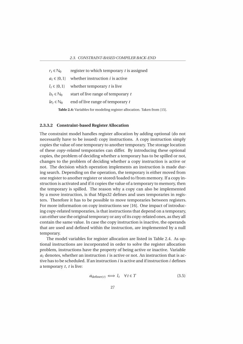
Table 2.4: Variables for modeling register allocation. Taken from [15].
2.3.3.2 Constraint-based Register Allocation
The constraint model handles register allocation by adding optional (do notnecessarily have to be issued) copy instructions. A copy instruction simplycopies the value of one temporary to another temporary. The storage locationof these copy-related temporaries can differ. By introducing these optionalcopies, the problem of deciding whether a temporary has to be spilled or not,changes to the problem of deciding whether a copy instruction is active ornot. The decision which operation implements an instruction is made dur-ing search. Depending on the operation, the temporary is either moved fromone register to another register or stored/loaded to/from memory. If a copy in-struction is activated and if it copies the value of a temporary to memory, thenthe temporary is spilled. The reason why a copy can also be implementedby a move instruction, is that Mips32 defines and uses temporaries in regis-ters. Therefore it has to be possible to move temporaries between registers.For more information on copy instructions see [16]. One impact of introduc-ing copy-related temporaries, is that instructions that depend on a temporary,can either use the original temporary or any of its copy-related ones, as they allcontain the same value. In case the copy instruction is inactive, the operandsthat are used and defined within the instruction, are implemented by a nulltemporary.
The model variables for register allocation are listed in Table 2.4. As op-tional instructions are incorporated in order to solve the register allocationproblem, instructions have the property of being active or inactive. Variableai denotes, whether an instruction i is active or not. An instruction that is ac-tive has to be scheduled. If an instruction i is active and if instruction i definesa temporary t , t is live:
adefiner(t ) ⇐⇒ lt ∀t ∈ T (3.5)
27
CHAPTER 2. BACKGROUND
A temporary t that is live has to implement an operand that is used by aninstruction, otherwise, the temporary would be dispensable:
lt ⇐⇒ ∃p : use(p)∧ tp = t ∀t ∈ T (3.6)
A live temporary has a live range that starts with the issue cycle of its definer.Let T be the set of temporaries and lt the Boolean value, which is set to one ift is live. For every t ∈ T , if lt = 1, then the following constraint enforces thatthe start of a temporary’s live range l st is equivalent to the issue cycle of itsdefiner:
lt =⇒ lst = cdefiner(t ) ∀t ∈ T (3.7)
Registers can only store one temporary at a time. For all temporaries that haveoverlapping live ranges and reside in a register, it has to be enforced that noregister is shared. A temporary’s live range starts at issue cycle l st and endsat issue cycle let . For every temporary that is live (lt = 1), the following con-straint enforces distinct live ranges for temporaries that are stored in the sameregister:
disjoint2({
⟨rt , lst , let , lt ⟩ : t ∈ tmp(b)}
) ∀b ∈ B (3.8)
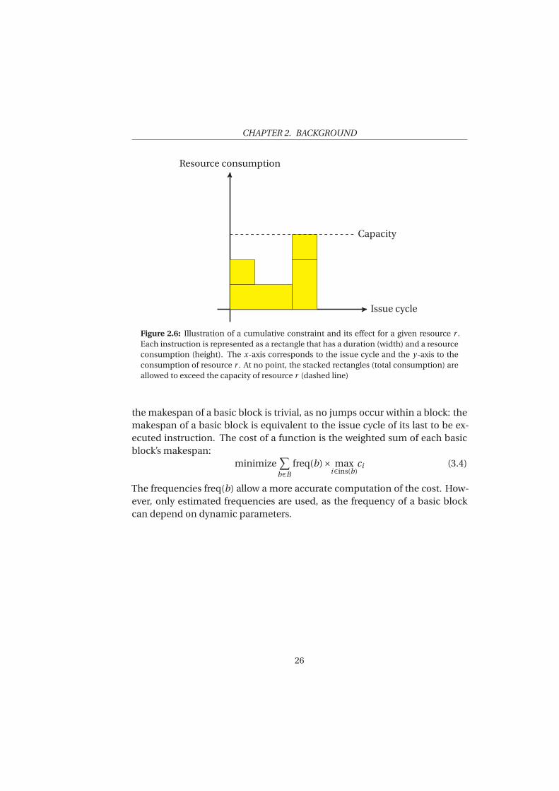
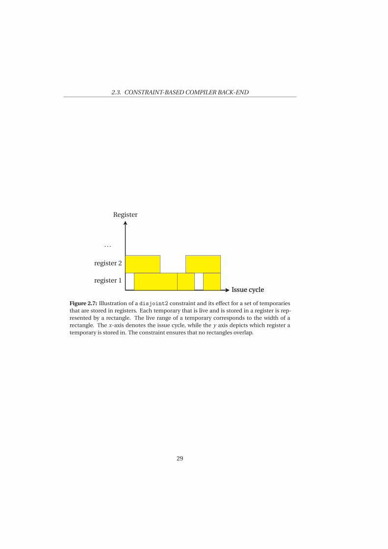
The disjoint2 constraint makes sure that live ranges of temporaries do notoverlap as registers can only store one temporary at a time. Figure 2.7 showsa valid assignment of temporaries to registers. Each rectangle correspondsto one live temporary that resides in one out of the two registers. A rectan-gle’s width represents the temporary’s live range. The disjoint2 constraintenforces that for each register, rectangles cannot overlap, or else one registerwould have to store multiple temporaries at the same issue cycle, which isinvalid.
For each pair of operands that is congruent (p ≡ q), the correspondingtemporaries tp that implement those operands have to reside in the same reg-ister:
rtp = rtq ∀p, q ∈ P : p ≡ q (3.9)
For each pre-assignment p⊲r of an operand p to a register r , a pre-assignmentconstraint enforces that the temporary tp that implements operand p will bestored in the pre-assigned register:
rtp = r ∀p ∈ P : p⊲r (3.10)
28
2.3. CONSTRAINT-BASED COMPILER BACK-END
Issue cycleIssue cycle
Register
register 1
register 2
. . .
Figure 2.7: Illustration of a disjoint2 constraint and its effect for a set of temporariesthat are stored in registers. Each temporary that is live and is stored in a register is rep-resented by a rectangle. The live range of a temporary corresponds to the width of arectangle. The x-axis denotes the issue cycle, while the y axis depicts which register atemporary is stored in. The constraint ensures that no rectangles overlap.
29
CH
AP
TE
R
3IMPLIED CONSTRAINTS
This chapter introduces implied constraints that are investigated in the con-text of the constraint-based compiler back-end. In order to find implied con-straints, a top-down approach was chosen: the constraints were elaboratedon existing literature.
The predecessor and successor constraints address precedences among in-structions and are described in Section 3.1. In Section 3.2 copy activation
constraints are introduced, which enforce a number of optional copy instruc-tions of a temporary to be active. Finally, Section 3.3 presents the nogood
constraints that detect infeasible partial assignments of subsets of variables,which can be used to avoid dead-ends during search.
3.1 Predecessor and Successor Constraints
In [18], Malik et al. present a constraint model for solving instruction schedul-ing on a multiple-issue processor. They accomplish to solve more realisticproblems amongst others by adding a number of implied constraints to theirbasic model. One idea they introduce are the predecessor and successor con-
straints.The predecessor constraints and their symmetric successor constraints
are based on the correlation between an instruction i and its immediate pre-decessors/successors. If an instruction i depends on the temporary that isdefined by another instruction j , j is referred to as an immediate predecessorof i . Respectively, i is an immediate successor of j . The reasoning behind thepredecessor constraints is the following: If an instruction i has a set of imme-
30
3.1. PREDECESSOR AND SUCCESSOR CONSTRAINTS
diate predecessors pred(i ), it can only be scheduled as soon as all predecessors
j ∈ pred(i ) complete execution. This implies that each instruction j ∈ pred(i )has consumed a resource without conflicting with any other predecessors’ re-source requirements. Malik et al. assume a unit duration for all instructions,i.e. dur(i ) = 1 ∀i ∈ I . Predecessor constraints are added for each type of func-tional unit r and each subset of P ∈ pred(i ) that consumes r if the total con-sumption exceeds the capacity of a resource r, |P | > cap(r ):
lower(ci ) ≥ min{lower(c j ) | j ∈ P }
+⌈
|P |/cap(r )⌉
−1
+min{lat( j ) | j ∈ P }
In other words, the earliest possible issue cycle of i is dependent on four fac-tors:
1. the earliest possible start time of a predecessor in P ,
2. the number of cycles |P | needed to issue all instructions in P ,
3. the maximum duration of all instructions in P (which is one), and
4. the minimum latency between a predecessor and instruction i .
Both term one and two of the equation are self explanatory. The last two termsrelate to the last to be executed predecessor jl ast . Instruction i depends onthe result produced by jl ast , thus it cannot be executed before the result isavailable (latency), but before jl ast finishes execution (duration). As it is notknown yet, which predecessor will be the last one to be executed, the maxi-mum duration is subtracted (third term) and the minimum latency is added(fourth term).
At this stage, the presented predecessor constraint assumes that all in-structions have a duration of one. The constraint model in this project, how-ever, supports instructions that may have a duration of more than one. Inorder to adapt the predecessor constraints, the notion of varying duration hasto be captured. Instead of adding a predecessor constraint for every subset P
for which the absolute number of predecessors |P | is greater than the capacity,the adapted predecessor constraints are added if the total usage of a resourcer is exceeded:
∑
j∈P
dur( j ,r )∗con( j ,r ) > cap(r )
31
CHAPTER 3. IMPLIED CONSTRAINTS
The term dur( j ,r )∗con( j ,r ) describes the total number of issue cycles that apredecessor j ∈ P requires in order to finish execution and thus the time inwhich resource r is occupied. If the total sum exceeds the capacity cap(r ), thefollowing adapted predecessor constraint is added:
lower(ci ) ≥ min{lower(c j ) | j ∈ P }
+
È
Ì
Ì
Ì
Ì
∑
j∈Pdur( j ,r )∗con( j ,r )
cap(r )
É
Í
Í
Í
Í
−max{dur( j ,r ) | j ∈ P }
+min{lat( j ) | j ∈ P }
(1.1)
Since the duration is taken into consideration, |P | changes to dur( j ,r )∗con( j ,r )and the previous subtracted maximum duration of 1 is now max{dur( j ,r ) | j ∈
P }. As before, the last to be executed predecessor’s duration does not play arole, but rather its latency. For dur( j ,r ) = 1 and con( j ,r ) = 1 the extendedpredecessor constraint is equivalent to the one defined in [18].
Likewise, the symmetric version of the predecessor constraints in [18], i.e. thesuccessor constraints, can be adapted. For each resource type r and each sub-set P of succ(i ) with
∑
j∈Pdur( j ,r )∗con( j ,r ) > cap(r ), a successor constraint is
added to the model:
upper(ci ) ≤ max{upper(c j ) | j ∈ S}
−
È
Ì
Ì
Ì
Ì
∑
j∈Sdur( j ,r )∗con( j ,r )
cap(r )
É
Í
Í
Í
Í
+max{dur( j ,r ) | j ∈ S}
−min{lat( j ) | j ∈ S}
(1.2)
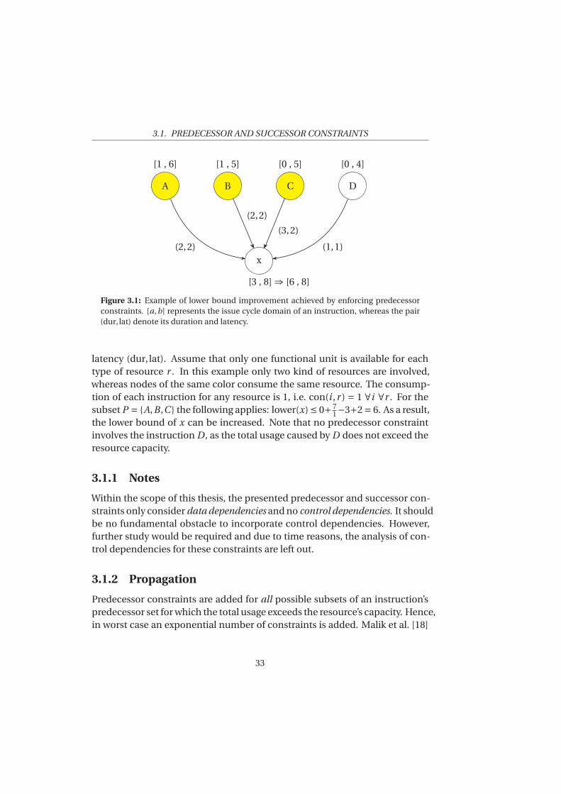
Example 3.1.1. Figure 3.1 shows an example result of enforcing predeces-sor constraints for an arbitrary instruction x and its immediate predecessors.Nodes represent instructions and edges define given data dependencies be-tween two nodes. The node color defines which kind of functional unit an in-struction’s operation consumes. Thus, if two instructions have the same color,they are executed by the same functional unit. Each instruction is defined byits issue cycle domain ci = [a,b] and its resource consumption duration and
32
3.1. PREDECESSOR AND SUCCESSOR CONSTRAINTS
A
[1 , 6]
B
[1 , 5]
C
[0 , 5]
D
[0 , 4]
x
[3 , 8] ⇒ [6 , 8]
(2,2)
(2,2)
(3,2)
(1,1)
Figure 3.1: Example of lower bound improvement achieved by enforcing predecessorconstraints. [a,b] represents the issue cycle domain of an instruction, whereas the pair(dur, lat) denote its duration and latency.
latency (dur, lat). Assume that only one functional unit is available for eachtype of resource r . In this example only two kind of resources are involved,whereas nodes of the same color consume the same resource. The consump-tion of each instruction for any resource is 1, i.e. con(i ,r ) = 1 ∀i ∀r . For thesubset P = {A,B ,C } the following applies: lower(x) ≤ 0+ 7
1−3+2 = 6. As a result,the lower bound of x can be increased. Note that no predecessor constraintinvolves the instruction D , as the total usage caused by D does not exceed theresource capacity.
3.1.1 Notes
Within the scope of this thesis, the presented predecessor and successor con-straints only consider data dependencies and no control dependencies. It shouldbe no fundamental obstacle to incorporate control dependencies. However,further study would be required and due to time reasons, the analysis of con-trol dependencies for these constraints are left out.
3.1.2 Propagation
Predecessor constraints are added for all possible subsets of an instruction’spredecessor set for which the total usage exceeds the resource’s capacity. Hence,in worst case an exponential number of constraints is added. Malik et al. [18]
33
CHAPTER 3. IMPLIED CONSTRAINTS
propose a heuristic that adds a total of O(
|I |2)
constraints instead, with |I | be-ing the total number of instructions. For each instruction i , the set of prede-cessors pred(i ) is sorted in the order of each predecessor’s lower bound. Next,a constraint is added for the whole set of predecessors. Then, the first prede-cessor is removed and a constraint is added for the remaining ones. Continueuntil only one predecessor is left. In other words, only one constraint is addedfor each subset size of |P |. Since only a number of subsets is considered, it isdesirable to pick the most effective ones. By removing the approximate ear-liest instruction, the heuristic aims at a high value for min{lower( j ) | j ∈ P },which sets the baseline for how many values can be pruned from an instruc-tion’s domain.
The approach of sorting the instructions according to their lower bound isnot appropriate for the constraint model in focus. At the time when predeces-sor constraints are generated, the lower bounds of all instructions are equiv-alent. Still, a similar approach can be applied: instead of sorting by lowerbound, pred(i ) can be sorted by the number of predecessor of each prede-cessor, i.e. pred(pred(i )). Given two predecessors j and k with
∣
∣pred( j )∣
∣ >=∣
∣pred(k)∣
∣, the new heuristic assumes that j is more likely to be executed af-ter k. Combining this ordering with the approach in [18], only a number ofpredecessor constraints is added to the model.
3.2 Copy Activation Constraints
Copy activation constraints address both register allocation and instructionscheduling. The following constraints are investigated and developed on thebasic idea of Dependency Graph Transformations formulated in [15].
Architectural constraints and the Application Binary Interface (ABI) causepre-assignments of operands to registers [16]. Temporaries that implementa pre-assigned operand have thus to be stored in a specific register. In thiscase, the temporary is also said to be pre-assigned. If two live temporaries areassigned to the same register, conflicts might occur, in which one temporaryis overwritten by the other. In order to avoid live values to be overwritten,optional copy instructions can be activated. The constraints enforcing copyinstructions to be active are the copy activation constraints.
Duration and latency values are irrelevant for the analysis in focus. Hence,the dependency graphs in this chapter do not differentiate between instruc-
34
3.2. COPY ACTIVATION CONSTRAINTS
A
B
C
.. .
. . .
ti ⊲r
t j ⊲r
(a) Pre-assignment conflict due tomultiple assignments to register r .
A
B
C
CPY tc = ti
copy related: {ti , tc }
. . .
. . .
ti ⊲r
tc
t j ⊲r
(b) Conflict resolved by enforcing theactivation of a copy instruction.
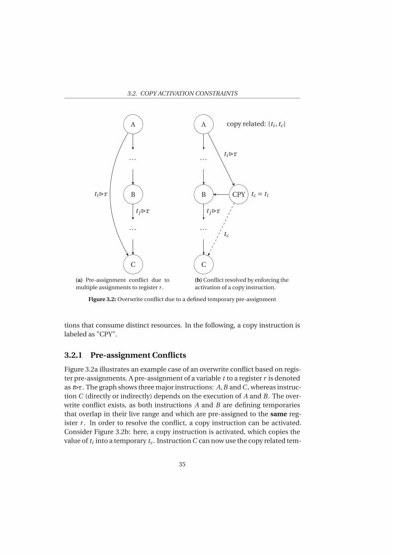
Figure 3.2: Overwrite conflict due to a defined temporary pre-assignment
tions that consume distinct resources. In the following, a copy instruction islabeled as "CPY".
3.2.1 Pre-assignment Conflicts
Figure 3.2a illustrates an example case of an overwrite conflict based on regis-ter pre-assignments. A pre-assignment of a variable t to a register r is denotedas t⊲r. The graph shows three major instructions: A,B and C , whereas instruc-tion C (directly or indirectly) depends on the execution of A and B . The over-write conflict exists, as both instructions A and B are defining temporariesthat overlap in their live range and which are pre-assigned to the same reg-ister r . In order to resolve the conflict, a copy instruction can be activated.Consider Figure 3.2b: here, a copy instruction is activated, which copies thevalue of ti into a temporary tc . Instruction C can now use the copy related tem-
35
CHAPTER 3. IMPLIED CONSTRAINTS
A
B
C ti ⊲r
. . .
. . .
ti
t j ⊲r
(a) Pre-assignment conflict due tomultiple assignments to register r .
A
B
C {tc , . . .}⊲r
CPY tc = ti
copy related: {ti , tc }
. . .
. . .
ti
tc⊲r
t j ⊲r
(b) Conflict resolved by enforcing theactivation of a copy instruction.
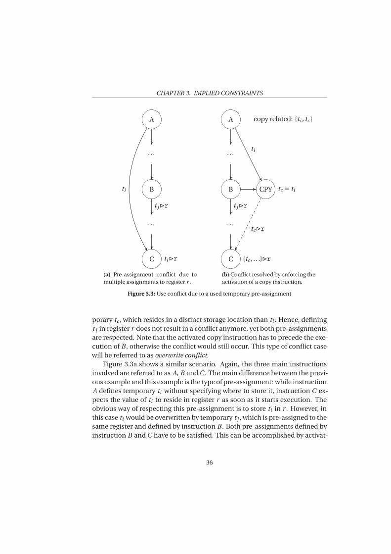
Figure 3.3: Use conflict due to a used temporary pre-assignment
porary tc , which resides in a distinct storage location than ti . Hence, definingt j in register r does not result in a conflict anymore, yet both pre-assignmentsare respected. Note that the activated copy instruction has to precede the exe-cution of B , otherwise the conflict would still occur. This type of conflict casewill be referred to as overwrite conflict.
Figure 3.3a shows a similar scenario. Again, the three main instructionsinvolved are referred to as A, B and C . The main difference between the previ-ous example and this example is the type of pre-assignment: while instructionA defines temporary ti without specifying where to store it, instruction C ex-pects the value of ti to reside in register r as soon as it starts execution. Theobvious way of respecting this pre-assignment is to store ti in r . However, inthis case ti would be overwritten by temporary t j , which is pre-assigned to thesame register and defined by instruction B . Both pre-assignments defined byinstruction B and C have to be satisfied. This can be accomplished by activat-
36
3.2. COPY ACTIVATION CONSTRAINTS
ing a copy instruction after the execution of instruction B : first instruction B
defines t j to be stored in register r ; afterward a copy instruction copies tem-porary ti into register r , see Figure 3.3b. This way, both pre-assignments donot conflict with each other. This type of conflict case will be referred to as use
conflict.
3.2.2 Formulation
The previous section introduced two types of conflicts that can occur dueto pre-assignments. By combining the information gathered from both over-write and use conflicts, one can deduce the total number of mandatory copy
instructions that have to be active for each temporary.A temporary that is affected by multiple overwrite conflicts within one
path of the dependency graph, only needs to be copied to another storagelocation once, i.e. before the first instruction in this path that causes an over-write conflict. If the temporary already resides in another location, all the fol-lowing overwrite conflicts are resolved. The same applies to use conflicts: atemporary needs to be copied to the pre-assigned storage location only once,namely after the last instruction in a path that causes a use conflict.
If a temporary pre-assignment is conflicting in several separate paths ofa dependency graph, it still needs to be copied over only once in order to besaved for all paths. In this case, however, it is not known beforehand which in-struction is the first or last one to cause the conflict (as they are not connectedby any dependency edge).
Combining the extracted knowledge from both cases, the total number ofmandatory copy instructions for one temporary can be summed up. If for agiven path only one out of the two possible conflicts occurs, the number ofmandatory copy instructions remains one. If however pre-assignments causeboth types of conflicts within one path of the dependency graph, the num-ber of mandatory copy instructions concerning a temporary might sum upto two. Let i → j denote that j is reachable from i in a given path. Assumefurthermore that the two instructions i and j are both involved in a distinctpre-assignment conflict concerning temporary t and that i → j without lossof generality. Then, the total number of mandatory copy instructions for tem-porary t is:
• one, if a copy is required after i and before j , and
• two, if a copy is required before i and after j .
37
CHAPTER 3. IMPLIED CONSTRAINTS
It is not required that i 6= j . One instruction alone can cause an overwrite anduse conflict at the same time, so that two copy instructions are required to beactive. One example is a call instruction that pre-assigns used temporaries aswell as defined temporaries:
[p2{t1}:$15] <- jalra [p1{t0}:$25]
The example function call instruction uses temporary t0 in register $25 andcomputes a temporary t1 that is pre-assigned to register $15. For example,requiring that t0 has to reside in register $25 can overwrite a temporary that isalready stored in that register (overwrite conflict) and defining a temporary tobe in register $15 might conflict with a following instruction that uses anothertemporary in register $15 (use conflict).
The final number of required copy instructions of a temporary t is the max-imum number of mandatory copy instructions that could be found among allpaths. Let ai denote that copy instruction i is active and thus has to be sched-uled. For each temporary t , the set of copy instructions C that copy t to an-other location and a number n = {1,2} of mandatory copy instructions, add acopy activation constraint:
∑
i∈C
ai ≥ n (2.3)
In other words, at least n copy instructions have to be active for a correct pro-gram flow. More copy instructions may be activated during search.
3.2.3 Notes
Apart from the main constraint in Equation 2.3, another minor constraint canbe formulated using the information gained from the copy activation analy-sis. It relates to the issue cycle of the out-delimiter, i.e. the makespan. Byconsidering the number of mandatory copy instructions and the number ofalready known to be issued instructions, one can impose a lower bound con-straint on the makespan. The makespan cannot be less than the number ofissue cycles required for executing all these obligatory instructions. As it isunknown beforehand, which operation is going to implement a copy instruc-tion, it is neither decided which resource is consumed nor how much of it isconsumed. All the instructions can nevertheless be used in order to computea minimum makespan: every instruction uses a part of the bundle rbundle ,
38
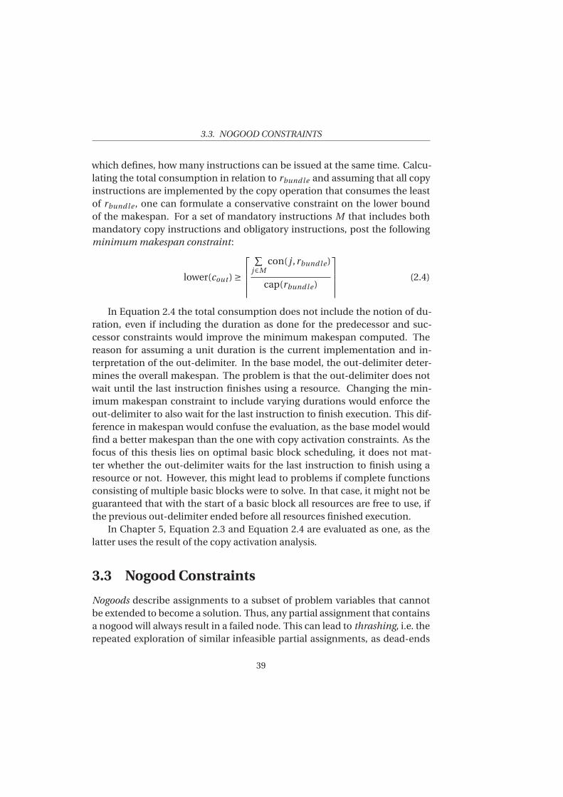
3.3. NOGOOD CONSTRAINTS
which defines, how many instructions can be issued at the same time. Calcu-lating the total consumption in relation to rbundle and assuming that all copyinstructions are implemented by the copy operation that consumes the leastof rbundle , one can formulate a conservative constraint on the lower boundof the makespan. For a set of mandatory instructions M that includes bothmandatory copy instructions and obligatory instructions, post the followingminimum makespan constraint:
lower(cout ) ≥
È
Ì
Ì
Ì
Ì
∑
j∈Mcon( j ,rbundle )
cap(rbundle )
É
Í
Í
Í
Í
(2.4)
In Equation 2.4 the total consumption does not include the notion of du-ration, even if including the duration as done for the predecessor and suc-cessor constraints would improve the minimum makespan computed. Thereason for assuming a unit duration is the current implementation and in-terpretation of the out-delimiter. In the base model, the out-delimiter deter-mines the overall makespan. The problem is that the out-delimiter does notwait until the last instruction finishes using a resource. Changing the min-imum makespan constraint to include varying durations would enforce theout-delimiter to also wait for the last instruction to finish execution. This dif-ference in makespan would confuse the evaluation, as the base model wouldfind a better makespan than the one with copy activation constraints. As thefocus of this thesis lies on optimal basic block scheduling, it does not mat-ter whether the out-delimiter waits for the last instruction to finish using aresource or not. However, this might lead to problems if complete functionsconsisting of multiple basic blocks were to solve. In that case, it might not beguaranteed that with the start of a basic block all resources are free to use, ifthe previous out-delimiter ended before all resources finished execution.
In Chapter 5, Equation 2.3 and Equation 2.4 are evaluated as one, as thelatter uses the result of the copy activation analysis.
3.3 Nogood Constraints
Nogoods describe assignments to a subset of problem variables that cannotbe extended to become a solution. Thus, any partial assignment that containsa nogood will always result in a failed node. This can lead to thrashing, i.e. therepeated exploration of similar infeasible partial assignments, as dead-ends
39
CHAPTER 3. IMPLIED CONSTRAINTS
within a search tree are not recognized as such. Nogoods are usually recordedduring backtracking search: if infeasible decisions lead to a failure, these de-cisions are recorded as a nogood in the hope that future dead-ends are dis-covered on time. Beek [26] gives an overview on nogood recording duringbacktracking search.
This project presents a static approach of finding nogoods for the codegeneration problem on hand. The general idea is to analyze a subset of prob-lem variables, their domains and relations among each other, prior to solvingthe complete code generation problem using CP. A nogood is thereby formu-lated as a conjunction of unit nogoods, i.e. nogoods of the form x = 3. Any no-good that is found during the analysis can be avoided during search by addinga corresponding constraint to the constraint model.
The nogoods that are to be detected are related to the subset of variablesthat determine operand-temporary assignments. Section 3.3.1 describes theproblem and introduces the methodology that is used in Section 3.3.2 andSection 3.3.3 for detecting nogoods.
3.3.1 Nogoods and the Boolean Satisfiability Problem
The sub-problem in focus is the task of deciding which temporary should im-plement an operand. Operands may be pre-assigned to registers, so that thetemporary implementing that operand has to be stored in that register. Byassigning a temporary to an operand, possible contradictions on the basis ofpre-assignments can occur. Consider the following simplistic example of anogood caused by an operand-temporary assignment. Given a temporary t ,registers r,k and two operands p, q whereas p⊲r, q⊲k. Both p and q can beimplemented by t or any copy-related temporary. However, defining that t im-plements both is invalid, as it implies that t should reside in register r and in k
at the same time, which conflicts with the requirement that t can only residein one register, if at all. By capturing existing operand-temporary relations,given pre-assignments and congruences, one can formulate a system of equa-tions that has to be satisfied. If adding a new operand-temporary assignmentsleads to a contradiction within the system, a nogood is found. Carlsson [3]proposes this idea of nogoods arising from operand-temporary assignments.
The system of equations can by implemented by using a variety of method-ologies. For instance, it can be viewed as a CP problem, in which assign-ments made that lead to a failed node are recorded as nogoods. In the contextof this thesis, the system of equations is modeled as a Boolean Satisfiability
40
3.3. NOGOOD CONSTRAINTS
(SAT) problem instance. SAT describes the problem of determining whether aBoolean formula is satisfiable, i.e. if Boolean value assignments exist, so thatthe formula evaluates to true. A Boolean formula consists of a set of liter-
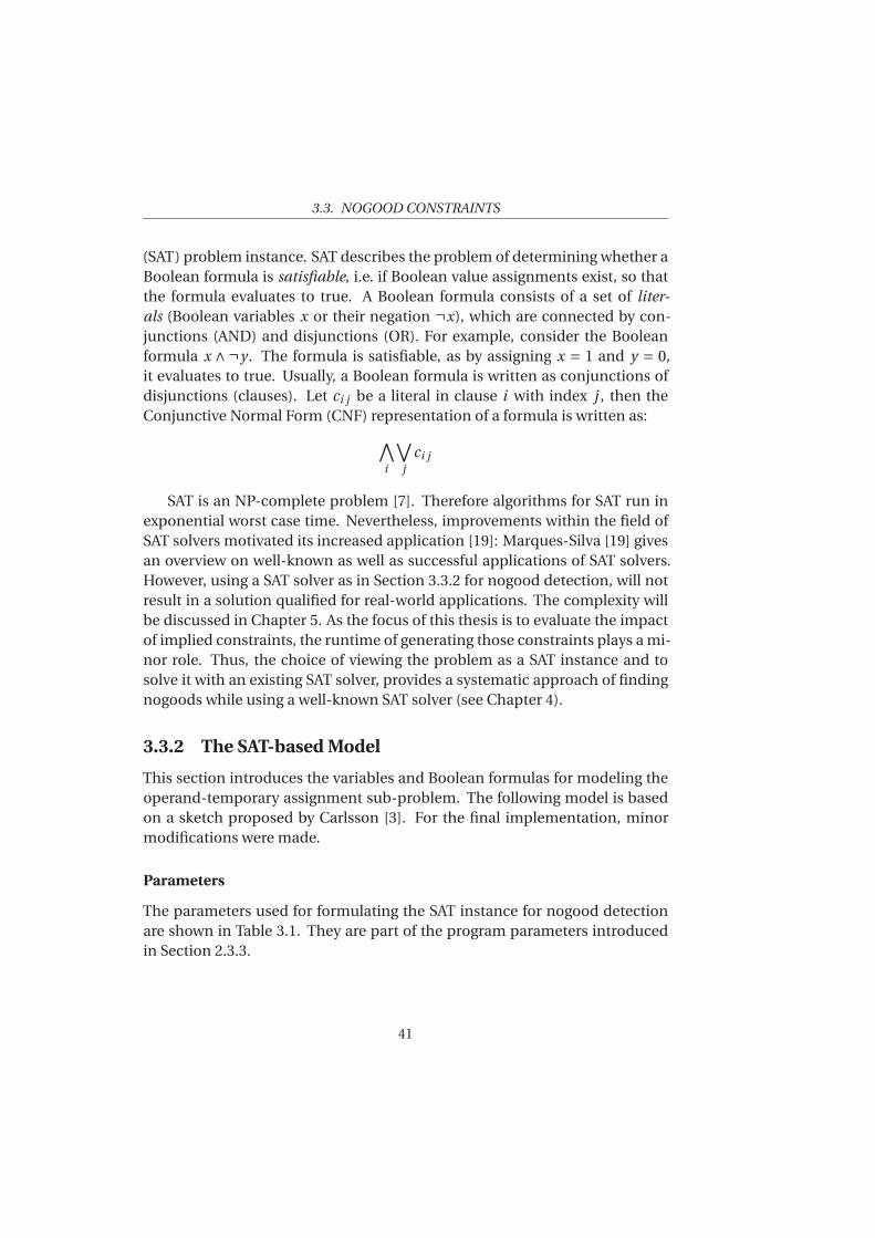
als (Boolean variables x or their negation ¬x), which are connected by con-junctions (AND) and disjunctions (OR). For example, consider the Booleanformula x ∧¬y . The formula is satisfiable, as by assigning x = 1 and y = 0,it evaluates to true. Usually, a Boolean formula is written as conjunctions ofdisjunctions (clauses). Let ci j be a literal in clause i with index j , then theConjunctive Normal Form (CNF) representation of a formula is written as:
∧
i
∨
j
ci j
SAT is an NP-complete problem [7]. Therefore algorithms for SAT run inexponential worst case time. Nevertheless, improvements within the field ofSAT solvers motivated its increased application [19]: Marques-Silva [19] givesan overview on well-known as well as successful applications of SAT solvers.However, using a SAT solver as in Section 3.3.2 for nogood detection, will notresult in a solution qualified for real-world applications. The complexity willbe discussed in Chapter 5. As the focus of this thesis is to evaluate the impactof implied constraints, the runtime of generating those constraints plays a mi-nor role. Thus, the choice of viewing the problem as a SAT instance and tosolve it with an existing SAT solver, provides a systematic approach of findingnogoods while using a well-known SAT solver (see Chapter 4).
3.3.2 The SAT-based Model
This section introduces the variables and Boolean formulas for modeling theoperand-temporary assignment sub-problem. The following model is basedon a sketch proposed by Carlsson [3]. For the final implementation, minormodifications were made.
Parameters
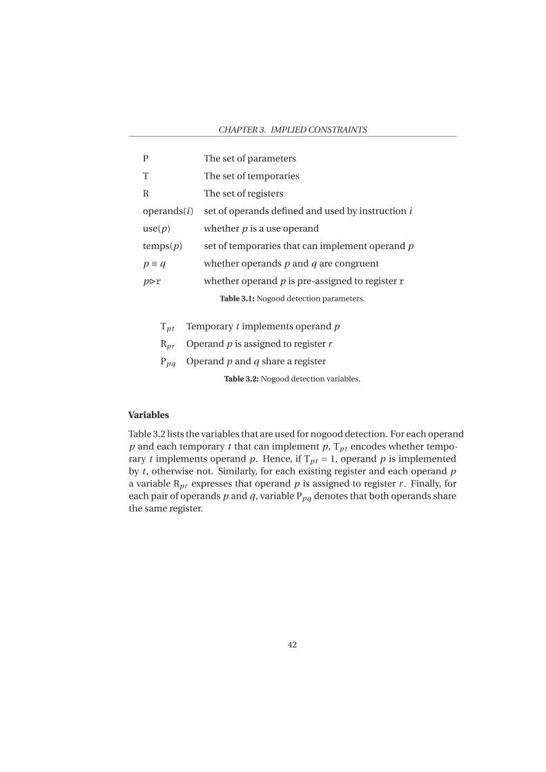
The parameters used for formulating the SAT instance for nogood detectionare shown in Table 3.1. They are part of the program parameters introducedin Section 2.3.3.
41
CHAPTER 3. IMPLIED CONSTRAINTS
P The set of parameters
T The set of temporaries
R The set of registers
operands(i ) set of operands defined and used by instruction i
use(p) whether p is a use operand
temps(p) set of temporaries that can implement operand p
p ≡ q whether operands p and q are congruent
p⊲r whether operand p is pre-assigned to register r
Table 3.1: Nogood detection parameters.
Tpt Temporary t implements operand p
Rpr Operand p is assigned to register r
Ppq Operand p and q share a register
Table 3.2: Nogood detection variables.
Variables
Table 3.2 lists the variables that are used for nogood detection. For each operandp and each temporary t that can implement p, Tpt encodes whether tempo-rary t implements operand p. Hence, if Tpt = 1, operand p is implementedby t , otherwise not. Similarly, for each existing register and each operand p
a variable Rpr expresses that operand p is assigned to register r . Finally, foreach pair of operands p and q , variable Ppq denotes that both operands sharethe same register.
42
3.3. NOGOOD CONSTRAINTS
The Constraints
In the following, each constraint is presented, followed by an equivalent for-mulation as a Boolean formula. The final Boolean formula that represents thesystem of equations is a conjunction of all presented formulas. For a morecompact representation, implications are written as a → b, which is a shorterversion of ¬a ∨b.
The first two constraints ensure the correctness of the base problem: eachoperand can only be implemented by one temporary and reside in maximumone register (if not stored in register, it is stored in main memory).
one temporary: each operand has to be implemented by exactly one tempo-rary.
exactlyOne(Tpt ) ∀p ∈ P (3.5)
at most one register: each operand can reside in only one register, if at all.
atMostOne(Rpt ) ∀p ∈ P (3.6)
The at-most-one constraint is implemented as described in [19]. For n vari-ables, it uses n − 1 auxiliary variables in order to express the constraint. Bycombining the at-most-one constraint with an at-least one constraint, onecan model the exactly-one constraint [19]. The at-least-one constraint for vari-ables xi can be expressed with the following clause:
∨
ixi
Some operands are already defined to share the same register and/or to re-side in a specific register. These assignments are known to be true, thereforethe corresponding variables are set:
congruences: congruent operands reside in the same register.
Ppq ∀p, q ∈ P : p ≡ q (3.7)
pre-assignments: A pre-assigned operand has to reside in the correspondingregister.
Rpr ∀p ∈ P : p⊲r (3.8)
43
CHAPTER 3. IMPLIED CONSTRAINTS
The following constraints provide rules to conclude assignments on a sub-set of variables if a premise is fulfilled. By defining a new operand-temporaryassignment, multiple of these premises may become true, so that new variable-value assignments are deduced that might conflict with already existing ones:
shared register transitivity: If an operand q shares a register with p and withs, operands p and s also share a register.
Ppq ∧Pqs → Pps ∀p, q, s ∈ P (3.9)
implied register assignment: If two operands are congruent and one operandis stored in a register, the other operand has to reside in the same register..
Ppq ∧Rpr → Rqr ∀r ∈ R, ∀p, q ∈ P (3.10)
implied shared register: If two operands reside in the same register, theyshare a register.
Rpr ∧Rqr → Ppq ∀r ∈ R, ∀p, q ∈ P (3.11)
distinct use registers: Each two pair of use operands within one instructionthat do not share temporaries, have to reside in distinct registers, as they arelive at the same time.
¬Ppq ∀i ∈ I ,
∀p, q ∈ operands(i ) :
use(p)∧use(q)∧ temps(p)∩ temps(q) =;
(3.12)
distinct define registers: Each two pair of defined operands within one in-struction that do not share temporaries, have to reside in distinct registers, asthey are live at the same time.
¬Ppq ∀i ∈ I ,
∀p, q ∈ operands(i ) :
¬use(p)∧¬use(q)
(3.13)
effective copy: In a copy instruction, the defined and used operand have toreside in different registers.
¬Psrc(i )dst(i ) ∀i ∈ I : type(i ) = copy, (3.14)
wheresrc(i ) = p : p ∈ operands(i )∧use(p)
dst(i ) = p : p ∈ operands(i )∧¬use(p)(3.15)
44
3.3. NOGOOD CONSTRAINTS
3.3.3 Detecting Nogoods
Nogoods are found by adding clauses representing operand-temporary as-signments. By adding a clause Tpt , one makes the assumption that a tempo-rary t implements an operand p. If the new assumption causes the formula tobecome unsatisfiable, a nogood is found. Nogoods can consist of one or mul-tiple operand-temporary assignments that are expressed by conjunctions ofassumptions Tpt . Within this project, only unit and binary nogoods are con-sidered, as the search for ternary nogoods using this approach takes too muchtime.
The number of combinations of operand-temporary assignment growswith the number of operands and thus with the number of instructions. Ifcomputing unit nogoods, one has to consider O
(
|P | ∗ |T |)
possible assump-tions: one assumption for each pair of an operand p and temporary t ∈ temps(p).For binary nogoods, there are already O
(
(|P | ∗ |T |)2)
combinations to test. Inany case, not all possible assumptions are necessarily reasonable. Only as-sumptions that might allow further conclusions on the system of equationsshould be considered. Otherwise, no conflict will be caused. An example foran assumption that is superfluous to consider if added alone is the follow-ing: consider an operand pc that is defined by an optional copy instruction.Operands that are defined by a copy instruction may be implemented by thenull temporary or by a real temporary tc . An assumption Tpc tc won’t causeany further conclusions if added alone, as the temporary tc is neither used byany other instruction nor does it pre-assign operand pc to any register. Thus,the total amount of tested assumptions can be reduced. In the following, thethesis describes the design choices and the incremental search used for pre-venting unnecessary checks of assumptions.
No null temporary implementation: As the assignment of any operand to anull temporary will not affect any other operand-temporary assignment, themodel only considers Boolean variables Tpt , for which t 6= null . This has theeffect that all optional copy instructions are assumed to be active (as the de-fined operand is not implemented by a null temporary).
Assumption only made for not yet assigned operands: Some operands canonly be implemented by one temporary. Consequently there is no need to addan assumption for those operands.
45
CHAPTER 3. IMPLIED CONSTRAINTS
Incremental search for nogoods: A nogood n1 subsumes a nogood n2, iff n1
is a subset of n2. In order to avoid adding subsumed nogoods, assumptionsare tested incrementally. First, unit assumptions are made. Only if the result-ing Boolean formula is still satisfiable, that assumption is recorded. For thegeneration of binary assumptions, the recorded unit assumptions are pairedup.
Add unit assumptions only if they concern mandatory operands: The deci-sion of which temporary shall implement an operand in an optional copy in-struction is not of interest, as it does not affect any other operand-temporaryassignment, if added alone. Thus, in terms of unit assumptions, the focus liesonly on mandatory operands (operands that are used/defined by a manda-tory instruction).
Add unit assumptions only for a subset of temporaries: Given a mandatoryoperand p, p can be implemented by any t ∈ temps(p). In order for a unitassumption to introduce a conflict, it has to bring in new information onoperand-register assignments. Assume that the temporary, which was definedoriginally, is pre-assigned to a register, i.e. to⊲r. Then, a temporary tc that is adirect copy of to cannot reside in r (Equation 3.14). For all other copy-relatedtemporaries that can either copy to (in r ) or tc (not in r ), it is not possible todeduce knowledge on where they might reside. Thus, for a given mandatoryoperand p, it is only relevant to consider the original temporary to or its directcopy tc .
Binary assumption only made if at least one mandatory operand is involved:Adding assumptions on operands of copy instructions only will not lead to anyconflict. Thus, at least one mandatory operand has to be considered.
Binary assumption only added if both operands are related: When consider-ing binary assumptions, the combined assumption can only have an effect, ifthey are related. Otherwise, adding both assumptions is equivalent to addingthem separately and in this case it is already known that these operands in iso-lation will not cause a conflict (incremental search). Let mandatory(p) denotethat operand p is part of a mandatory instruction. In this thesis, two operandsp and q are related if:
1. both are mandatory and may be implemented by the same temporary:
46
3.3. NOGOOD CONSTRAINTS
mandatory(p)∧mandatory(q)∧ temps(p)∩ temps(q) 6= ;,
2. both are mandatory use operands and belong to the same instruction:mandatory(p)∧mandatory(q)∧∃i : p, q ∈ use(i ), and
3. one is mandatory and it uses a temporary that is the result of copyingover the temporary that implements the other operand:w.l.o.g mandatory(p)∧¬mandatory(q)∧q = src(i ) : Tpt ∧Tdst(i )t .
Regarding the last point, note that only use operands of a copy instruction areyet undefined: by ignoring null temporaries, each defined operand of a copyinstruction is already implemented by a temporary.
Binary assumptions only added for a subset of temporaries: An obligatoryoperand can be implemented by a temporary to (the known to be active, origi-nal temporary), a copy-related temporary tc that directly copies over to , or anyother temporary ti whose copy source is either to or tc . From the viewpoint ofthis model, all temporaries of the latter kind are equivalent as they have thesame copy source options, even if they are not the same in the original con-straint model. Any nogood that contains the temporary ti can be translatedto a nogood for any other copy-related temporary that has t0 and tc as a copysource. Hence, instead of considering all equivalent temporaries, the thesisonly focuses on one representative of this group of copy related temporaries.
By this adaptions the amount of generated assumptions can be reduced.Nevertheless, the complexity can only be reduced by a constant. Chapter 4will present the SAT solver used within this project and Chapter 5 will analyzethe runtime of the nogood detection.
3.3.4 Formulation
A nogood consists of a set of operand-temporary assignments tp = t , which to-gether form an infeasible partial assignment if all become true. For each suchnogood of size n = {1,2} (unit and binary nogoods), let B with |B | = n be theset of Boolean variables so that bi ⇐⇒ tpi
= ti ∀i ∈ {1 . . .n}. Then, a nogood
constraint is added:
∑
i
bi < n (3.16)
47
CH
AP
TE
R
4IMPLEMENTATION
The implementation is separated into a pre-processing and a constraint gen-eration part. The pre-processing for predecessor, successor and copy activa-tion constraints involves the construction and analysis of a dependency graphcontaining both data dependencies and control dependencies. Based on theresults of the graph analysis, the implied constraints are generated and addedto the constraint model. As the graph pre-processing is a part of the existingmodeler module written in Haskell, Haskell is the natural language of choice.The pre-processing for nogood generation is written in C++. It uses the SATsolver MiniSat 2.2.0 [22, 23] as a native library and is part of a pre-processingwithin the solver itself. Similarly, C++ is used for constraint generation sincethe existing solver is written in C++. It uses the open source toolkit Gecode3.7.3 [25] for the development of constraint-based systems. The following sec-tion outlines the structure of the constructed dependency graph and the ap-proach for detecting nogoods using MiniSat. It furthermore describes howthe information for adding the implied constraints from Chapter 3 can be ob-tained.
4.1 Dependency Graph
The dependency graph that is constructed contains only edges among manda-
tory instructions and thus does not consider precedences among optional copyinstructions. Edges can relate to data dependencies or control dependencies.An example dependency graph of one block contained in an actual test func-tion is shown in Figure 4.1. Solid edges represent data dependency edges.
48
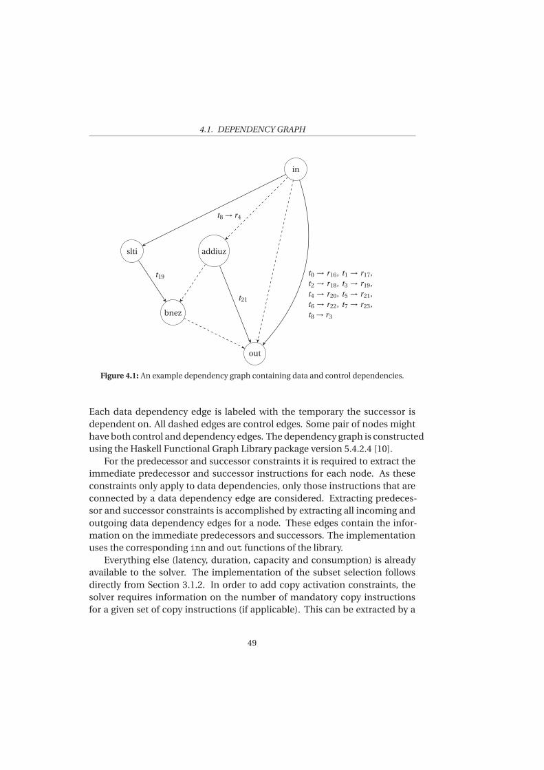
4.1. DEPENDENCY GRAPH
in
slti addiuz
bnez
out
t8 → r4
t19
t21
t0 → r16, t1 → r17,t2 → r18, t3 → r19,t4 → r20, t5 → r21,t6 → r22, t7 → r23,t8 → r3
Figure 4.1: An example dependency graph containing data and control dependencies.
Each data dependency edge is labeled with the temporary the successor isdependent on. All dashed edges are control edges. Some pair of nodes mighthave both control and dependency edges. The dependency graph is constructedusing the Haskell Functional Graph Library package version 5.4.2.4 [10].
For the predecessor and successor constraints it is required to extract theimmediate predecessor and successor instructions for each node. As theseconstraints only apply to data dependencies, only those instructions that areconnected by a data dependency edge are considered. Extracting predeces-sor and successor constraints is accomplished by extracting all incoming andoutgoing data dependency edges for a node. These edges contain the infor-mation on the immediate predecessors and successors. The implementationuses the corresponding inn and out functions of the library.
Everything else (latency, duration, capacity and consumption) is alreadyavailable to the solver. The implementation of the subset selection followsdirectly from Section 3.1.2. In order to add copy activation constraints, thesolver requires information on the number of mandatory copy instructionsfor a given set of copy instructions (if applicable). This can be extracted by a
49
CHAPTER 4. IMPLEMENTATION
graph analysis that will be described in the following section.
4.1.1 Graph Analysis
The graph analysis concerns the detection of overwrite and use conflicts asdescribed in Section 3.2. A simplified version of the algorithm is listed inAlgorithm 4.1, which uses two procedures for collecting the conflicts: Proce-dure extractOverwriteConflicts is used for overwrite conflicts, whereas Proce-dure extractUseConflicts detects use conflicts. Detecting overwrite conflictsstarts off with extracting all instructions that define pre-assigned temporariesin Line 1. For each instruction, the pre-assigned temporaries and registers areobtained in Line 2 and Line 3. Now, for each path that starts at the given in-struction, conflicts are detected that occur along that path. A conflict exists ifany instruction along that path uses the same registers as the ones obtainedbefore. The result of the analysis in Line 5 is a collection of conflict tuples thatdescribe a conflict by:
1. the instruction that causes the conflict,
2. the temporary that has to be copied, and
3. the time, when a copy instruction has to be active.
The time is specified in relation to the instruction that causes the conflict.Therefore, a copy instruction has to be active either before or after the conflict-ing instruction is issued. Extracting use conflicts is processed in a symmetricway, see Procedure extractUseConflicts. The analysis of overwrite and use con-flicts has a complexity of O
(
|I |∗|IP |∗rm
)
, with IP being the set of instructionsthat contain pre-assignments, rm being the number of machine registers and|IP |≪ |I |. The number of instructions contained in IP is considerably smallerthan the number of instructions contained in I , as a large number of instruc-tions are optional copy instructions that do not have any pre-assignments.
The conflict tuples of both analyses are combined in Algorithm 4.1. InLine 4, stricter conflicts are filtered: for each path at most one overwrite con-flict tuple and at most one use conflict tuple has to be kept, as suggestedin Section 3.2.2. It is only necessary to copy once before the earliest over-write conflict and once after the latest use conflict. Line 5 computes the num-ber of mandatory copy instructions for each temporary as described in Sec-
50
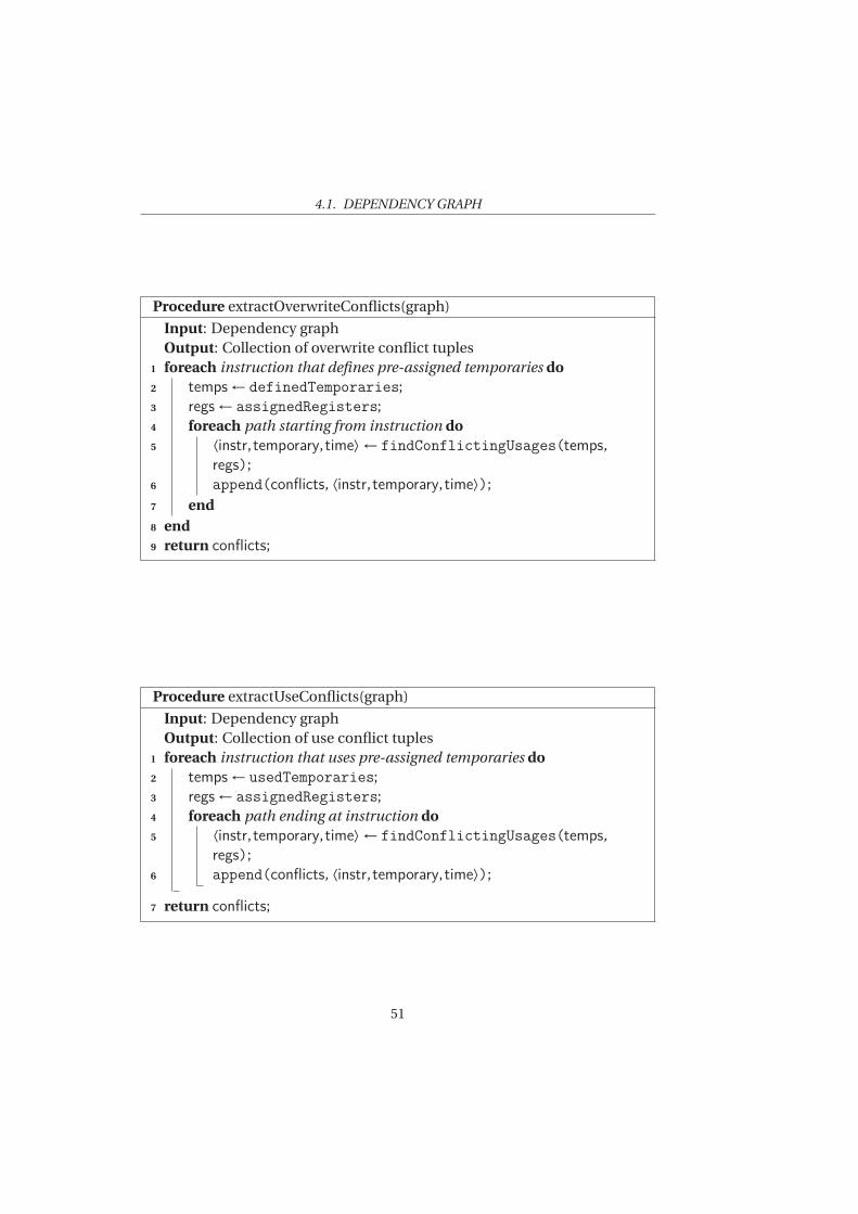
4.1. DEPENDENCY GRAPH
Procedure extractOverwriteConflicts(graph)
Input: Dependency graphOutput: Collection of overwrite conflict tuples
1 foreach instruction that defines pre-assigned temporaries do
2 temps ← definedTemporaries;3 regs ← assignedRegisters;4 foreach path starting from instruction do
5 ⟨instr,temporary,time⟩ ← findConflictingUsages(temps,
regs);6 append(conflicts, ⟨instr,temporary,time⟩);
7 end
8 end
9 return conflicts;
Procedure extractUseConflicts(graph)
Input: Dependency graphOutput: Collection of use conflict tuples
1 foreach instruction that uses pre-assigned temporaries do
2 temps ← usedTemporaries;3 regs ← assignedRegisters;4 foreach path ending at instruction do
5 ⟨instr,temporary,time⟩ ← findConflictingUsages(temps,
regs);6 append(conflicts, ⟨instr,temporary,time⟩);
7 return conflicts;
51
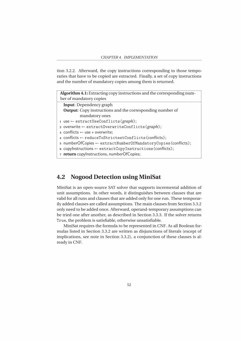
CHAPTER 4. IMPLEMENTATION
tion 3.2.2. Afterward, the copy instructions corresponding to those tempo-raries that have to be copied are extracted. Finally, a set of copy instructionsand the number of mandatory copies among them is returned.
Algorithm 4.1: Extracting copy instructions and the corresponding num-ber of mandatory copies
Input: Dependency graphOutput: Copy instructions and the corresponding number of
mandatory ones1 use ← extractUseConflicts(graph);2 overwrite ← extractOverwriteConflicts(graph);3 conflicts ← use + overwrite;4 conflicts ← reduceToStrictestConflicts(conflicts);5 numberOfCopies ← extractNumberOfMandatoryCopies(conflicts);6 copyInstructions ← extractCopyInstructions(conflicts);7 return copyInstructions, numberOfCopies;
4.2 Nogood Detection using MiniSat
MiniSat is an open-source SAT solver that supports incremental addition ofunit assumptions. In other words, it distinguishes between clauses that arevalid for all runs and clauses that are added only for one run. These temporar-ily added clauses are called assumptions. The main clauses from Section 3.3.2only need to be added once. Afterward, operand-temporary assumptions canbe tried one after another, as described in Section 3.3.3. If the solver returnsTrue, the problem is satisfiable, otherwise unsatisfiable.
MiniSat requires the formula to be represented in CNF. As all Boolean for-mulas listed in Section 3.3.2 are written as disjunctions of literals (except ofimplications, see note in Section 3.3.2), a conjunction of these clauses is al-ready in CNF.
52
CH
AP
TE
R
5EVALUATION
This chapter focuses on the evaluation of the impact of the introduced im-plied constraints on the code generation problem. In this thesis, the impactof constraints is measured in relation to the base constraint model. The com-parative measurement is based on the number of failed nodes that are en-countered during search until the optimal solution is found. The more failednodes, the more time is spent exploring infeasible partial solutions. By com-paring the difference in the number of failed nodes for the base model andone that is extended with an implied constraint, one can draw conclusions ontheir effect on cutting down the search effort.
How well an implied constraint performs, is dependent on several factors.If a constraint that is successful in reducing the search overhead in one set-up, it does not imply that the same will happen for every other set-up. As thecontext plays a major role for a constraint’s effectiveness, it is required to takethe context into account in order to identify the strengths and weaknesses ofa constraint. Thus, the questions to answer within this chapter are:
1. If applicable, how do the implied constraints help to cut down the searcheffort?
2. How do the implied constraints interact with each other?
3. For which variants of the Mips32 architecture do the implied constraintshave the most or the least impact?
4. What role does the search heuristic play?
53
CHAPTER 5. EVALUATION
As the first question suggests, the experiments focus on the Mips32 archi-tecture and variants of it that are obtained by slight alternations of architec-tural characteristics. Due to a lack of time the experiments are not run for dis-tinct architectural back-ends than the Mips32. The analysis of search heuris-tics is out of scope, however, some insights on the influence of the searchheuristic on an implied constraint’s impact can be drawn, so that parts ofquestion number four can be answered. For simplicity, the hardness of a prob-lem instance is seen relatively to the search effort that was required for thebase model to find the optimal solution.
In order to answer the questions in focus, several experiments are run. Sec-tion 5.1 delineates the experimental set up, i.e. the test instances, the searchheuristic and the extracted data from each run. Section 5.2 analyzes resultsgained for the unaltered Mips32 architecture, both for adding single constraintsand for adding groups of constraints. Section 5.3, Section 5.4 and Section 5.5concentrate on the impact of single constraints for variants of the Mips32.
5.1 Experimental Set Up
The test set contains 1176 basic blocks that were extracted from 94 test func-tions. The test functions belong to the C program bzip2, which is part of thestandard SPEC CPU2006 benchmark suite [13]. Each basic block is solved in-dependently and is thus to be seen as a stand-alone test instance.
During the experiments, the following two values are extracted for eachtest instance:
1. Solution cost (makespan) and
2. Number of failed nodes encountered until finding the solution.
The thesis does not contain the measurement of runtime. Measuring thenumber of failed nodes instead gives the possibility to measure the impactplatform-independently. On top of that, as the search heuristic is almost com-pletely static, approximately the same sequence of nodes will be explored. Ifa failed node is detected a part of that sequence is just skipped. Therefore,measuring the number of failed nodes goes along with the runtime neededfor finding the solution.
All experiments are run on a Linux machine with an Intel Core 2 Duo pro-cessor P8700 with 2.9 GiB of memory. The experimental set up imposes a time-out of 30 seconds on the search. The applied search heuristic is configured to
54
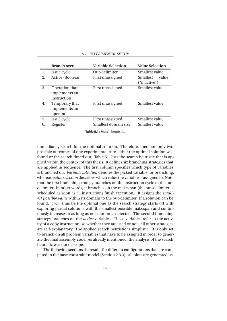
5.1. EXPERIMENTAL SET UP
Branch over Variable Selection Value Selection
1. Issue cycle Out-delimiter Smallest value2. Active (Boolean) First unassigned Smallest value
("inactive")3. Operation that
implements aninstruction
First unassigned Smallest value
4. Temporary thatimplements anoperand
First unassigned Smallest value
5. Issue cycle First unassigned Smallest value6. Register Smallest domain size Smallest value
Table 5.1: Search heuristic.
immediately search for the optimal solution. Therefore, there are only twopossible outcomes of one experimental run: either the optimal solution wasfound or the search timed out. Table 5.1 lists the search heuristic that is ap-plied within the context of this thesis. It defines six branching strategies thatare applied in sequence. The first column specifies which type of variablesis branched on. Variable selection denotes the picked variable for branching,whereas value selection describes which value the variable is assigned to. Notethat the first branching strategy branches on the instruction cycle of the out-delimiter. In other words, it branches on the makespan (the out-delimiter isscheduled as soon as all instructions finish execution). It assigns the small-
est possible value within its domain to the out-delimiter. If a solution can befound, it will thus be the optimal one as the search strategy starts off withexploring partial solutions with the smallest possible makespan and contin-uously increases it as long as no solution is detected. The second branchingstrategy branches on the active variables. These variables refer to the activ-ity of a copy instruction, so whether they are used or not. All other strategiesare self-explanatory. The applied search heuristic is simplistic. It is only setto branch on all problem variables that have to be assigned in order to gener-ate the final assembly code. As already mentioned, the analysis of the searchheuristic was out of scope.
The following sections list results for different configurations that are com-pared to the base constraint model (Section 2.3.3). All plots are generated us-
55
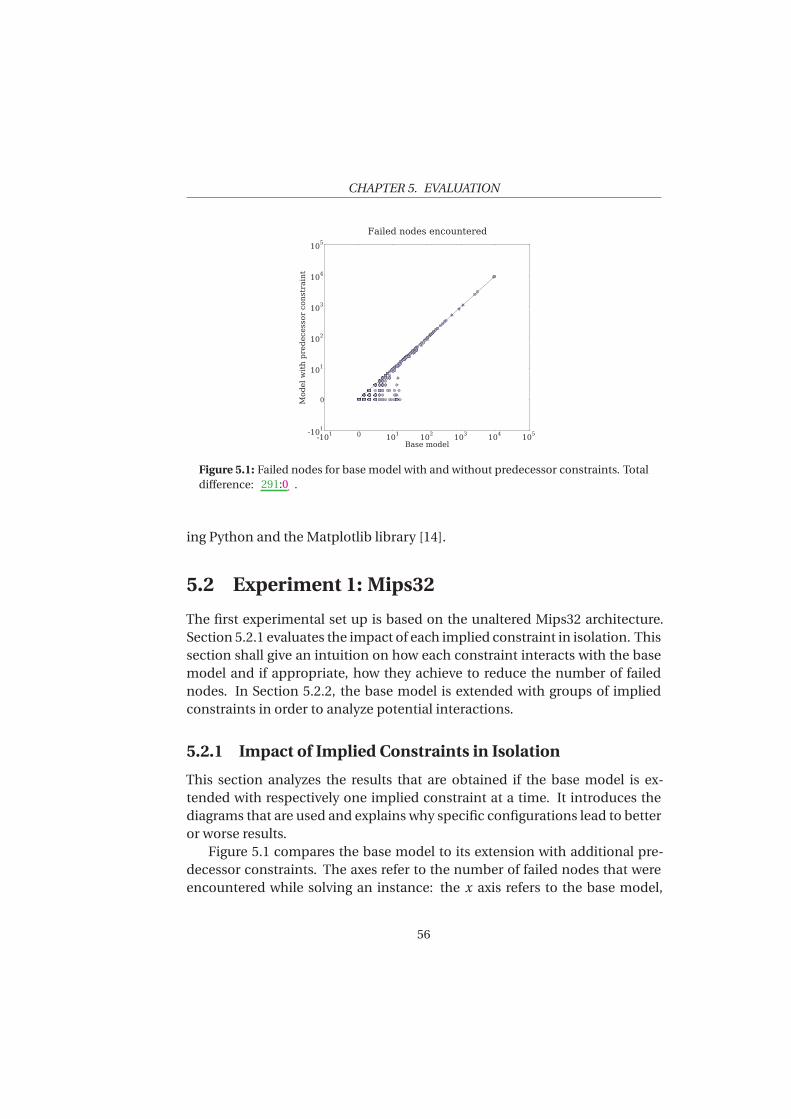
CHAPTER 5. EVALUATION
-10
1
0
10
1
10
2
10
3
10
4
10
5
Base model
-10
1
0
10
1
10
2
10
3
10
4
10
5
Model w
ith predecessor constraint
Failed nodes encountered
Figure 5.1: Failed nodes for base model with and without predecessor constraints. Totaldifference: 291:0 .
ing Python and the Matplotlib library [14].
5.2 Experiment 1: Mips32
The first experimental set up is based on the unaltered Mips32 architecture.Section 5.2.1 evaluates the impact of each implied constraint in isolation. Thissection shall give an intuition on how each constraint interacts with the basemodel and if appropriate, how they achieve to reduce the number of failednodes. In Section 5.2.2, the base model is extended with groups of impliedconstraints in order to analyze potential interactions.
5.2.1 Impact of Implied Constraints in Isolation
This section analyzes the results that are obtained if the base model is ex-tended with respectively one implied constraint at a time. It introduces thediagrams that are used and explains why specific configurations lead to betteror worse results.
Figure 5.1 compares the base model to its extension with additional pre-decessor constraints. The axes refer to the number of failed nodes that wereencountered while solving an instance: the x axis refers to the base model,
56
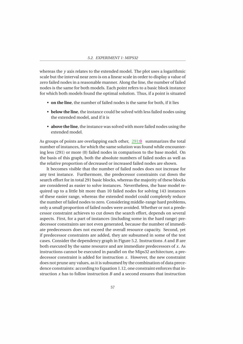
5.2. EXPERIMENT 1: MIPS32
whereas the y axis relates to the extended model. The plot uses a logarithmicscale but the interval near zero is on a linear scale in order to display a value ofzero failed nodes in a reasonable manner. Along the line, the number of failednodes is the same for both models. Each point refers to a basic block instancefor which both models found the optimal solution. Thus, if a point is situated
• on the line, the number of failed nodes is the same for both, if it lies
• below the line, the instance could be solved with less failed nodes usingthe extended model, and if it is
• above the line, the instance was solved with more failed nodes using theextended model.
As groups of points are overlapping each other, 291:0 summarizes the totalnumber of instances, for which the same solution was found while encounter-ing less (291) or more (0) failed nodes in comparison to the base model. Onthe basis of this graph, both the absolute numbers of failed nodes as well asthe relative proportion of decreased or increased failed nodes are shown.
It becomes visible that the number of failed nodes does not increase forany test instance. Furthermore, the predecessor constraints cut down thesearch effort for in total 291 basic blocks, whereas the majority of these blocksare considered as easier to solve instances. Nevertheless, the base model re-quired up to a little bit more than 10 failed nodes for solving 143 instancesof these easier range, whereas the extended model could completely reducethe number of failed nodes to zero. Considering middle-range hard problems,only a small proportion of failed nodes were avoided. Whether or not a prede-cessor constraint achieves to cut down the search effort, depends on severalaspects. First, for a part of instances (including some in the hard range) pre-decessor constraints are not even generated, because the number of immedi-ate predecessors does not exceed the overall resource capacity. Second, yetif predecessor constraints are added, they are subsumed in some of the testcases. Consider the dependency graph in Figure 5.2. Instructions A and B areboth executed by the same resource and are immediate predecessors of x. Asinstructions cannot be executed in parallel on the Mips32 architecture, a pre-decessor constraint is added for instruction x. However, the new constraintdoes not prune any values, as it is subsumed by the combination of data prece-dence constraints: according to Equation 1.12, one constraint enforces that in-struction x has to follow instruction B and a second ensures that instruction
57
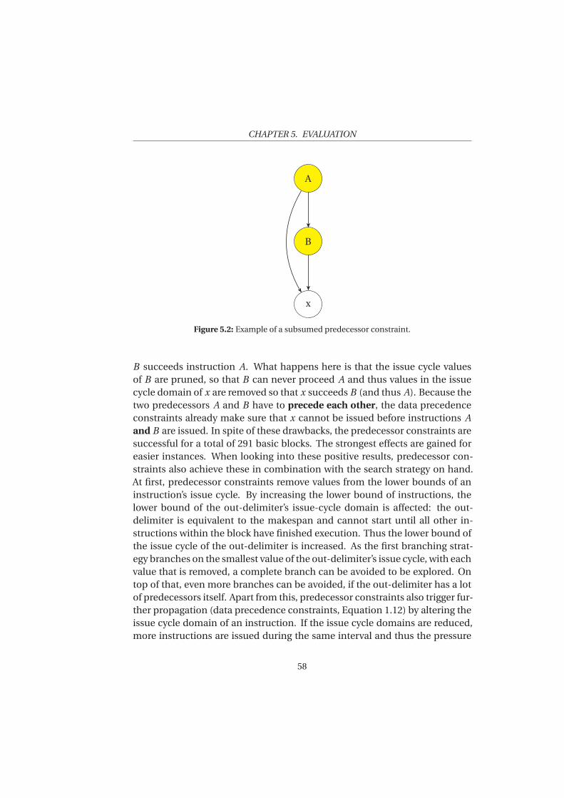
CHAPTER 5. EVALUATION
A
B
x
Figure 5.2: Example of a subsumed predecessor constraint.
B succeeds instruction A. What happens here is that the issue cycle valuesof B are pruned, so that B can never proceed A and thus values in the issuecycle domain of x are removed so that x succeeds B (and thus A). Because thetwo predecessors A and B have to precede each other, the data precedenceconstraints already make sure that x cannot be issued before instructions A
and B are issued. In spite of these drawbacks, the predecessor constraints aresuccessful for a total of 291 basic blocks. The strongest effects are gained foreasier instances. When looking into these positive results, predecessor con-straints also achieve these in combination with the search strategy on hand.At first, predecessor constraints remove values from the lower bounds of aninstruction’s issue cycle. By increasing the lower bound of instructions, thelower bound of the out-delimiter’s issue-cycle domain is affected: the out-delimiter is equivalent to the makespan and cannot start until all other in-structions within the block have finished execution. Thus the lower bound ofthe issue cycle of the out-delimiter is increased. As the first branching strat-egy branches on the smallest value of the out-delimiter’s issue cycle, with eachvalue that is removed, a complete branch can be avoided to be explored. Ontop of that, even more branches can be avoided, if the out-delimiter has a lotof predecessors itself. Apart from this, predecessor constraints also trigger fur-ther propagation (data precedence constraints, Equation 1.12) by altering theissue cycle domain of an instruction. If the issue cycle domains are reduced,more instructions are issued during the same interval and thus the pressure
58
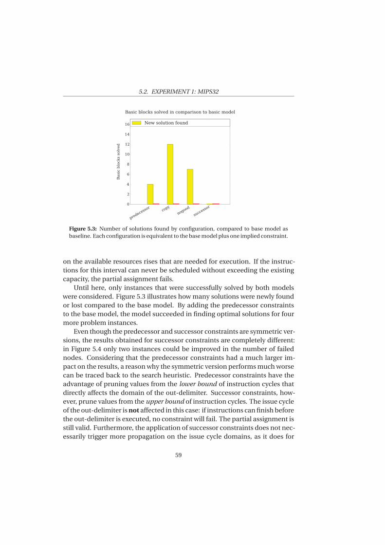
5.2. EXPERIMENT 1: MIPS32
p
r
e
d
e
c
e
s
s
o
r
c
o
p
y
n
o
g
o
o
d
s
u
c
c
e
s
s
o
r
0
2
4
6
8
10
12
14
16
Basic blocks solved
Basic blocks solved in comparison to basic model
New solution found
Figure 5.3: Number of solutions found by configuration, compared to base model asbaseline. Each configuration is equivalent to the base model plus one implied constraint.
on the available resources rises that are needed for execution. If the instruc-tions for this interval can never be scheduled without exceeding the existingcapacity, the partial assignment fails.
Until here, only instances that were successfully solved by both modelswere considered. Figure 5.3 illustrates how many solutions were newly foundor lost compared to the base model. By adding the predecessor constraintsto the base model, the model succeeded in finding optimal solutions for fourmore problem instances.
Even though the predecessor and successor constraints are symmetric ver-sions, the results obtained for successor constraints are completely different:in Figure 5.4 only two instances could be improved in the number of failednodes. Considering that the predecessor constraints had a much larger im-pact on the results, a reason why the symmetric version performs much worsecan be traced back to the search heuristic. Predecessor constraints have theadvantage of pruning values from the lower bound of instruction cycles thatdirectly affects the domain of the out-delimiter. Successor constraints, how-ever, prune values from the upper bound of instruction cycles. The issue cycleof the out-delimiter is not affected in this case: if instructions can finish beforethe out-delimiter is executed, no constraint will fail. The partial assignment isstill valid. Furthermore, the application of successor constraints does not nec-essarily trigger more propagation on the issue cycle domains, as it does for
59
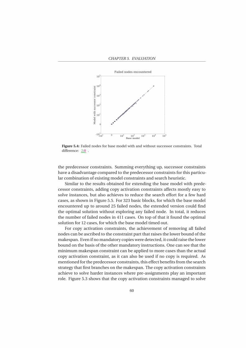
CHAPTER 5. EVALUATION
-10
1
0
10
1
10
2
10
3
10
4
10
5
Base model
-10
1
0
10
1
10
2
10
3
10
4
10
5
Model w
ith successor constraint
Failed nodes encountered
Figure 5.4: Failed nodes for base model with and without successor constraints. Totaldifference: 2:0 .
the predecessor constraints. Summing everything up, successor constraintshave a disadvantage compared to the predecessor constraints for this particu-lar combination of existing model constraints and search heuristic.
Similar to the results obtained for extending the base model with prede-cessor constraints, adding copy activation constraints affects mostly easy tosolve instances, but also achieves to reduce the search effort for a few hardcases, as shown in Figure 5.5. For 323 basic blocks, for which the base modelencountered up to around 25 failed nodes, the extended version could findthe optimal solution without exploring any failed node. In total, it reducesthe number of failed nodes in 411 cases. On top of that it found the optimalsolution for 12 cases, for which the base model timed out.
For copy activation constraints, the achievement of removing all failednodes can be ascribed to the constraint part that raises the lower bound of themakespan. Even if no mandatory copies were detected, it could raise the lowerbound on the basis of the other mandatory instructions. One can see that theminimum makespan constraint can be applied to more cases than the actualcopy activation constraint, as it can also be used if no copy is required. Asmentioned for the predecessor constraints, this effect benefits from the searchstrategy that first branches on the makespan. The copy activation constraintsachieve to solve harder instances where pre-assignments play an importantrole. Figure 5.3 shows that the copy activation constraints managed to solve
60
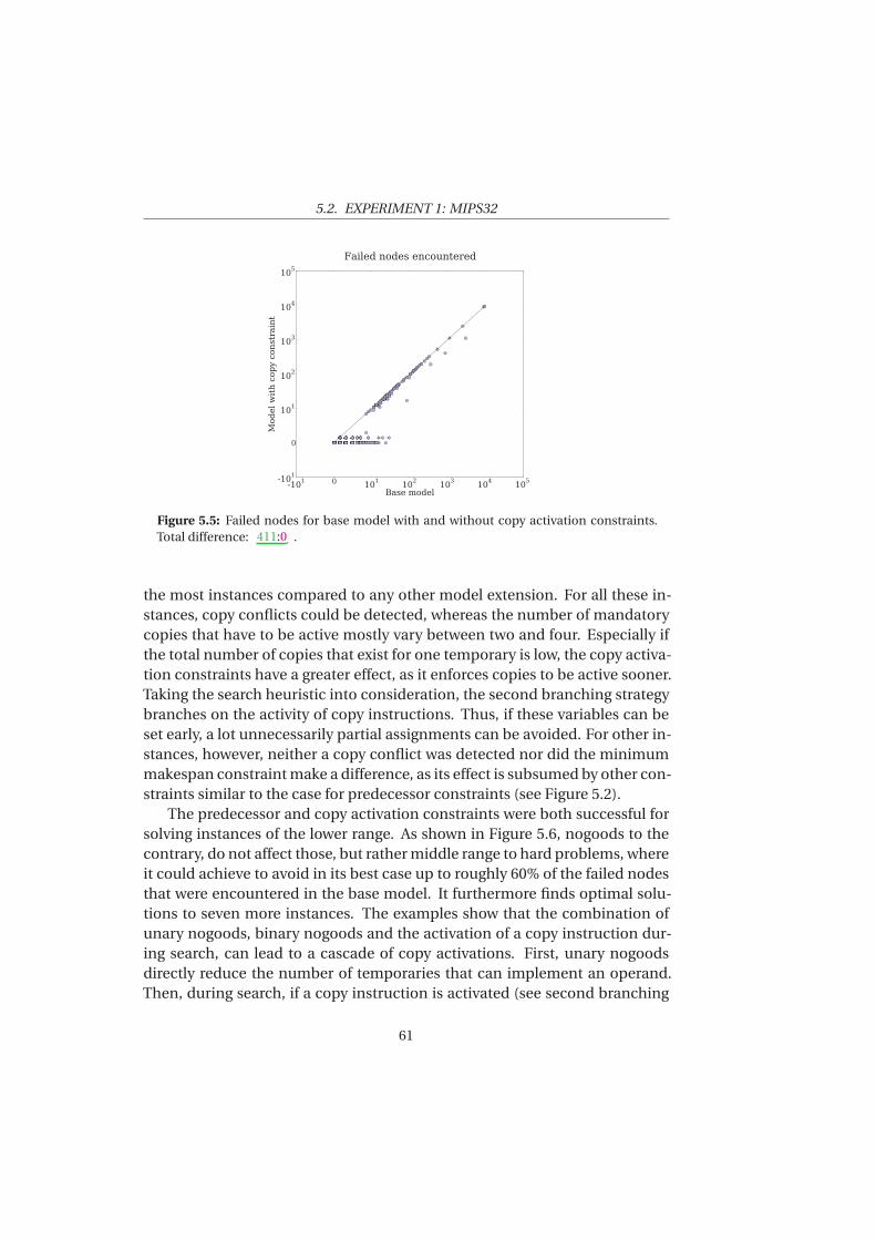
5.2. EXPERIMENT 1: MIPS32
-10
1
0
10
1
10
2
10
3
10
4
10
5
Base model
-10
1
0
10
1
10
2
10
3
10
4
10
5
Model w
ith copy constraint
Failed nodes encountered
Figure 5.5: Failed nodes for base model with and without copy activation constraints.Total difference: 411:0 .
the most instances compared to any other model extension. For all these in-stances, copy conflicts could be detected, whereas the number of mandatorycopies that have to be active mostly vary between two and four. Especially ifthe total number of copies that exist for one temporary is low, the copy activa-tion constraints have a greater effect, as it enforces copies to be active sooner.Taking the search heuristic into consideration, the second branching strategybranches on the activity of copy instructions. Thus, if these variables can beset early, a lot unnecessarily partial assignments can be avoided. For other in-stances, however, neither a copy conflict was detected nor did the minimummakespan constraint make a difference, as its effect is subsumed by other con-straints similar to the case for predecessor constraints (see Figure 5.2).
The predecessor and copy activation constraints were both successful forsolving instances of the lower range. As shown in Figure 5.6, nogoods to thecontrary, do not affect those, but rather middle range to hard problems, whereit could achieve to avoid in its best case up to roughly 60% of the failed nodesthat were encountered in the base model. It furthermore finds optimal solu-tions to seven more instances. The examples show that the combination ofunary nogoods, binary nogoods and the activation of a copy instruction dur-ing search, can lead to a cascade of copy activations. First, unary nogoodsdirectly reduce the number of temporaries that can implement an operand.Then, during search, if a copy instruction is activated (see second branching
61
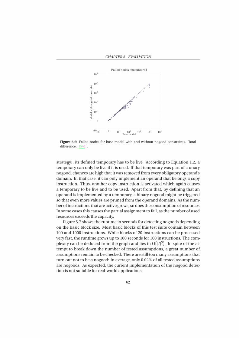
CHAPTER 5. EVALUATION
-10
1
0
10
1
10
2
10
3
10
4
10
5
Base model
-10
1
0
10
1
10
2
10
3
10
4
10
5
Model w
ith nogood constraint
Failed nodes encountered
Figure 5.6: Failed nodes for base model with and without nogood constraints. Totaldifference: 29:0 .
strategy), its defined temporary has to be live. According to Equation 1.2, atemporary can only be live if it is used. If that temporary was part of a unarynogood, chances are high that it was removed from every obligatory operand’sdomain. In that case, it can only implement an operand that belongs a copyinstruction. Thus, another copy instruction is activated which again causesa temporary to be live and to be used. Apart from that, by defining that anoperand is implemented by a temporary, a binary nogood might be triggeredso that even more values are pruned from the operand domains. As the num-ber of instructions that are active grows, so does the consumption of resources.In some cases this causes the partial assignment to fail, as the number of usedresources exceeds the capacity.
Figure 5.7 shows the runtime in seconds for detecting nogoods dependingon the basic block size. Most basic blocks of this test suite contain between100 and 1000 instructions. While blocks of 20 instructions can be processedvery fast, the runtime grows up to 100 seconds for 100 instructions. The com-plexity can be deduced from the graph and lies in O
(
|I |3)
. In spite of the at-tempt to break down the number of tested assumptions, a great number ofassumptions remain to be checked. There are still too many assumptions thatturn out not to be a nogood: in average, only 0.02% of all tested assumptionsare nogoods. As expected, the current implementation of the nogood detec-tion is not suitable for real-world applications.
62
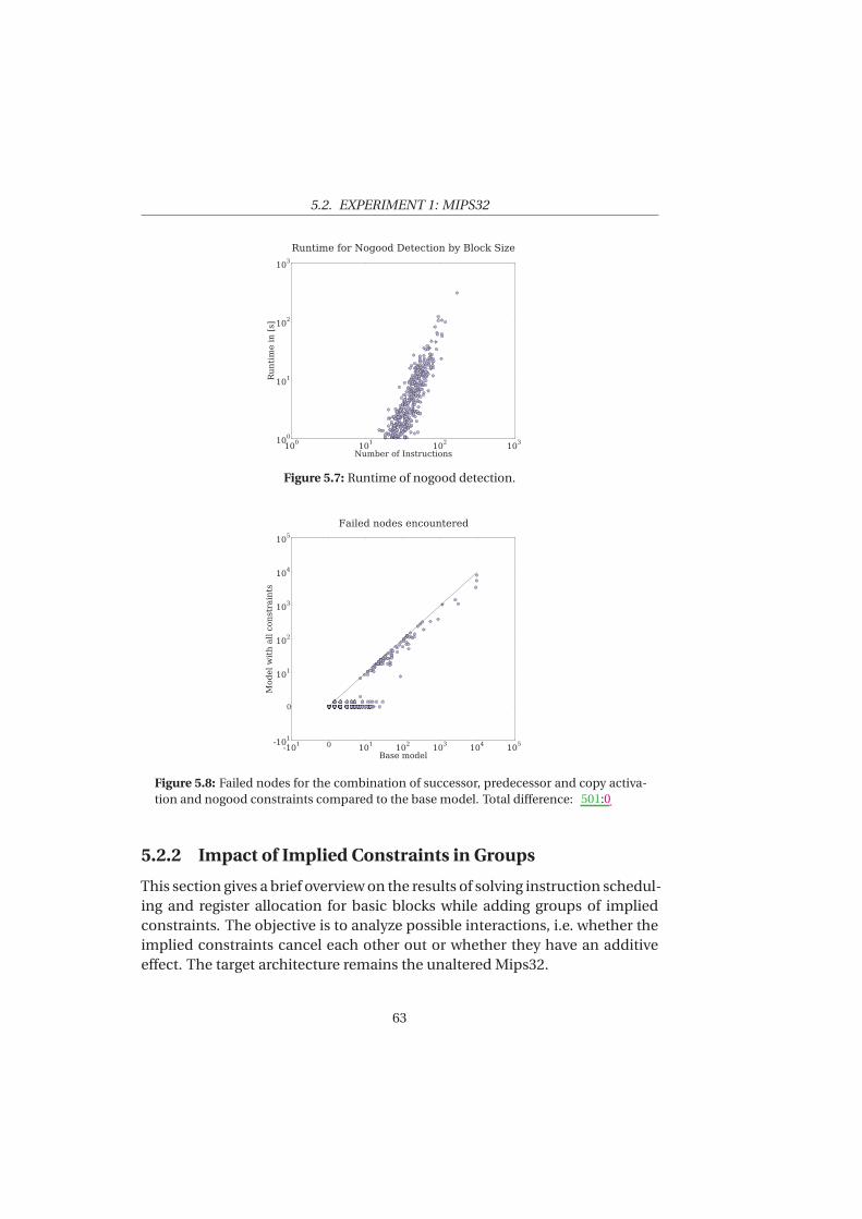
5.2. EXPERIMENT 1: MIPS32
10
0
10
1
10
2
10
3
Number of Instructions
10
0
10
1
10
2
10
3
Runtime in [s]
Runtime for Nogood Detection by Block Size
Figure 5.7: Runtime of nogood detection.
-10
1
0
10
1
10
2
10
3
10
4
10
5
Base model
-10
1
0
10
1
10
2
10
3
10
4
10
5
Model w
ith all constraints
Failed nodes encountered
Figure 5.8: Failed nodes for the combination of successor, predecessor and copy activa-tion and nogood constraints compared to the base model. Total difference: 501:0
5.2.2 Impact of Implied Constraints in Groups
This section gives a brief overview on the results of solving instruction schedul-ing and register allocation for basic blocks while adding groups of impliedconstraints. The objective is to analyze possible interactions, i.e. whether theimplied constraints cancel each other out or whether they have an additiveeffect. The target architecture remains the unaltered Mips32.
63
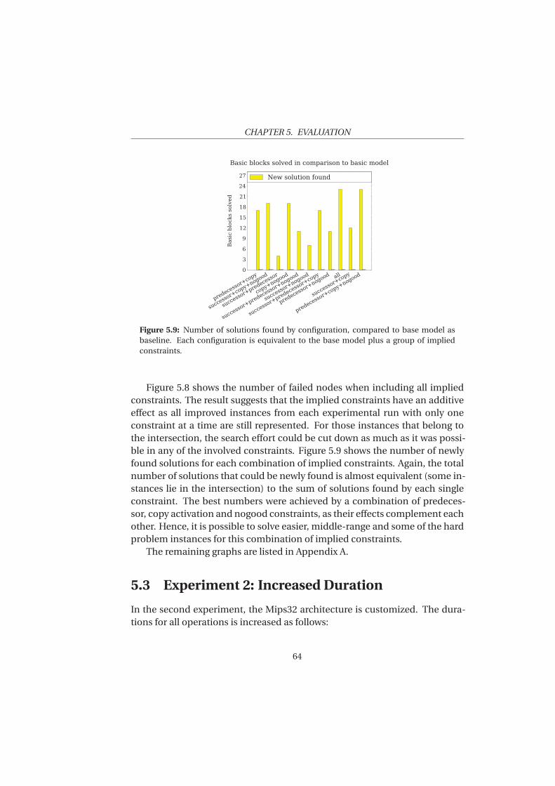
CHAPTER 5. EVALUATION
p
r
e
d
e
c
e
s
s
o
r
+
c
o
p
y
s
u
c
c
e
s
s
o
r
+
c
o
p
y
+
n
o
g
o
o
d
s
u
c
c
e
s
s
o
r
+
p
r
e
d
e
c
e
s
s
o
r
c
o
p
y
+
n
o
g
o
o
d
s
u
c
c
e
s
s
o
r
+
p
r
e
d
e
c
e
s
s
o
r
+
n
o
g
o
o
d
s
u
c
c
e
s
s
o
r
+
n
o
g
o
o
d
s
u
c
c
e
s
s
o
r
+
p
r
e
d
e
c
e
s
s
o
r
+
c
o
p
y
p
r
e
d
e
c
e
s
s
o
r
+
n
o
g
o
o
d
a
l
l
s
u
c
c
e
s
s
o
r
+
c
o
p
y
p
r
e
d
e
c
e
s
s
o
r
+
c
o
p
y
+
n
o
g
o
o
d
0
3
6
9
12
15
18
21
24
27
Basic blocks solved
Basic blocks solved in comparison to basic model
New solution found
Figure 5.9: Number of solutions found by configuration, compared to base model asbaseline. Each configuration is equivalent to the base model plus a group of impliedconstraints.
Figure 5.8 shows the number of failed nodes when including all impliedconstraints. The result suggests that the implied constraints have an additiveeffect as all improved instances from each experimental run with only oneconstraint at a time are still represented. For those instances that belong tothe intersection, the search effort could be cut down as much as it was possi-ble in any of the involved constraints. Figure 5.9 shows the number of newlyfound solutions for each combination of implied constraints. Again, the totalnumber of solutions that could be newly found is almost equivalent (some in-stances lie in the intersection) to the sum of solutions found by each singleconstraint. The best numbers were achieved by a combination of predeces-sor, copy activation and nogood constraints, as their effects complement eachother. Hence, it is possible to solve easier, middle-range and some of the hardproblem instances for this combination of implied constraints.
The remaining graphs are listed in Appendix A.
5.3 Experiment 2: Increased Duration
In the second experiment, the Mips32 architecture is customized. The dura-tions for all operations is increased as follows:
64
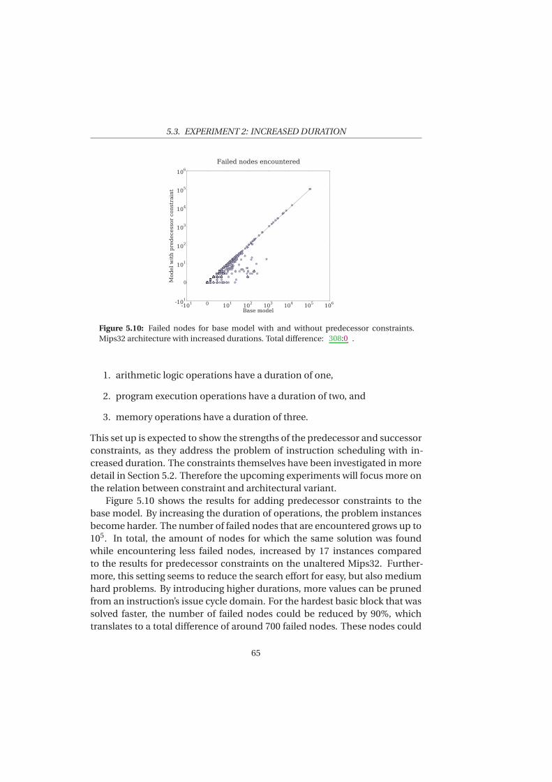
5.3. EXPERIMENT 2: INCREASED DURATION
-10
1
0
10
1
10
2
10
3
10
4
10
5
10
6
Base model
-10
1
0
10
1
10
2
10
3
10
4
10
5
10
6
Model with predecessor constraint
Failed nodes encountered
Figure 5.10: Failed nodes for base model with and without predecessor constraints.Mips32 architecture with increased durations. Total difference: 308:0 .
1. arithmetic logic operations have a duration of one,
2. program execution operations have a duration of two, and
3. memory operations have a duration of three.
This set up is expected to show the strengths of the predecessor and successorconstraints, as they address the problem of instruction scheduling with in-creased duration. The constraints themselves have been investigated in moredetail in Section 5.2. Therefore the upcoming experiments will focus more onthe relation between constraint and architectural variant.
Figure 5.10 shows the results for adding predecessor constraints to thebase model. By increasing the duration of operations, the problem instancesbecome harder. The number of failed nodes that are encountered grows up to105. In total, the amount of nodes for which the same solution was foundwhile encountering less failed nodes, increased by 17 instances comparedto the results for predecessor constraints on the unaltered Mips32. Further-more, this setting seems to reduce the search effort for easy, but also mediumhard problems. By introducing higher durations, more values can be prunedfrom an instruction’s issue cycle domain. For the hardest basic block that wassolved faster, the number of failed nodes could be reduced by 90%, whichtranslates to a total difference of around 700 failed nodes. These nodes could
65
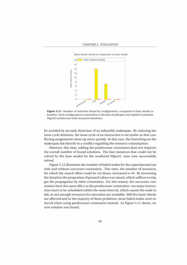
CHAPTER 5. EVALUATION
p
r
e
d
e
c
e
s
s
o
r
c
o
p
y
n
o
g
o
o
d
s
u
c
c
e
s
s
o
r
0
2
4
6
8
10
12
14
16
18
Basic blocks solved
Basic blocks solved in comparison to basic model
New solution found
Figure 5.11: Number of solutions found by configuration, compared to base model asbaseline. Each configuration is equivalent to the base model plus one implied constraint.Mips32 architecture with increased durations.
be avoided by an early detection of an infeasible makespan. By reducing theissue cycle domains, the issue cycle of an instruction is set earlier so that con-flicting assignments show up more quickly. In this case, the branching on themakespan led directly to a conflict regarding the resource consumption.
However, this time, adding the predecessor constraints does not improvethe overall number of found solutions. The four instances that could not besolved by the base model for the unaltered Mips32, were now successfullysolved.
Figure 5.12 illustrates the number of failed nodes for the experimental runwith and without successor constraints. This time, the number of instances,for which the search effort could be cut down, increased to 49. By increasingthe duration the proportion of pruned values was raised, which suffices to trig-ger the propagation by other constraints. For this reason, the successor con-straints have the same effect as the predecessor constraints: too many instruc-tions have to be scheduled within the same interval, which causes the node tofail, as not enough resources for execution are available. Still few basic blocksare affected and in the majority of these problems, more failed nodes were re-duced when using predecessor constraints instead. As Figure 5.11 shows, nonew solution was found.
66
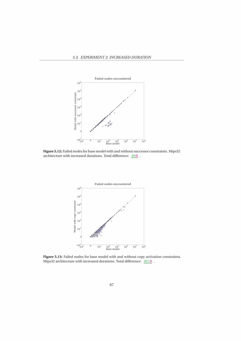
5.3. EXPERIMENT 2: INCREASED DURATION
-10
1
0
10
1
10
2
10
3
10
4
10
5
10
6
Base model
-10
1
0
10
1
10
2
10
3
10
4
10
5
10
6
Model w
ith successor constraint
Failed nodes encountered
Figure 5.12: Failed nodes for base model with and without successor constraints. Mips32architecture with increased durations. Total difference: 49:0 .
-10
1
0
10
1
10
2
10
3
10
4
10
5
10
6
Base model
-10
1
0
10
1
10
2
10
3
10
4
10
5
10
6
Model w
ith copy constraint
Failed nodes encountered
Figure 5.13: Failed nodes for base model with and without copy activation constraints.Mips32 architecture with increased durations. Total difference: 367:0 .
67
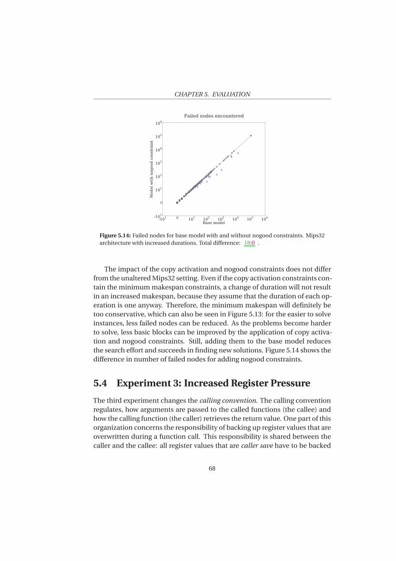
CHAPTER 5. EVALUATION
-10
1
0
10
1
10
2
10
3
10
4
10
5
10
6
Base model
-10
1
0
10
1
10
2
10
3
10
4
10
5
10
6
Model w
ith nogood constraint
Failed nodes encountered
Figure 5.14: Failed nodes for base model with and without nogood constraints. Mips32architecture with increased durations. Total difference: 18:0 .
The impact of the copy activation and nogood constraints does not differfrom the unaltered Mips32 setting. Even if the copy activation constraints con-tain the minimum makespan constraints, a change of duration will not resultin an increased makespan, because they assume that the duration of each op-eration is one anyway. Therefore, the minimum makespan will definitely betoo conservative, which can also be seen in Figure 5.13: for the easier to solveinstances, less failed nodes can be reduced. As the problems become harderto solve, less basic blocks can be improved by the application of copy activa-tion and nogood constraints. Still, adding them to the base model reducesthe search effort and succeeds in finding new solutions. Figure 5.14 shows thedifference in number of failed nodes for adding nogood constraints.
5.4 Experiment 3: Increased Register Pressure
The third experiment changes the calling convention. The calling conventionregulates, how arguments are passed to the called functions (the callee) andhow the calling function (the caller) retrieves the return value. One part of thisorganization concerns the responsibility of backing up register values that areoverwritten during a function call. This responsibility is shared between thecaller and the callee: all register values that are caller save have to be backed
68
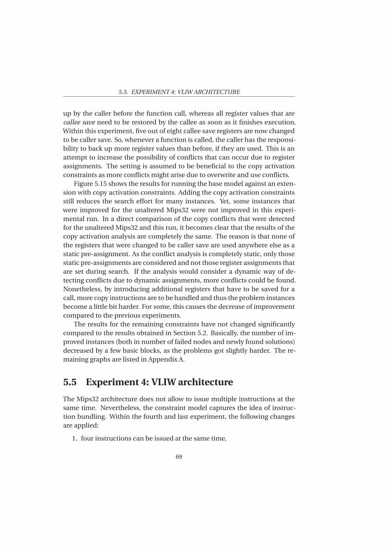
5.5. EXPERIMENT 4: VLIW ARCHITECTURE
up by the caller before the function call, whereas all register values that arecallee save need to be restored by the callee as soon as it finishes execution.Within this experiment, five out of eight callee save registers are now changedto be caller save. So, whenever a function is called, the caller has the responsi-bility to back up more register values than before, if they are used. This is anattempt to increase the possibility of conflicts that can occur due to registerassignments. The setting is assumed to be beneficial to the copy activationconstraints as more conflicts might arise due to overwrite and use conflicts.
Figure 5.15 shows the results for running the base model against an exten-sion with copy activation constraints. Adding the copy activation constraintsstill reduces the search effort for many instances. Yet, some instances thatwere improved for the unaltered Mips32 were not improved in this experi-mental run. In a direct comparison of the copy conflicts that were detectedfor the unaltered Mips32 and this run, it becomes clear that the results of thecopy activation analysis are completely the same. The reason is that none ofthe registers that were changed to be caller save are used anywhere else as astatic pre-assignment. As the conflict analysis is completely static, only thosestatic pre-assignments are considered and not those register assignments thatare set during search. If the analysis would consider a dynamic way of de-tecting conflicts due to dynamic assignments, more conflicts could be found.Nonetheless, by introducing additional registers that have to be saved for acall, more copy instructions are to be handled and thus the problem instancesbecome a little bit harder. For some, this causes the decrease of improvementcompared to the previous experiments.
The results for the remaining constraints have not changed significantlycompared to the results obtained in Section 5.2. Basically, the number of im-proved instances (both in number of failed nodes and newly found solutions)decreased by a few basic blocks, as the problems got slightly harder. The re-maining graphs are listed in Appendix A.
5.5 Experiment 4: VLIW architecture
The Mips32 architecture does not allow to issue multiple instructions at thesame time. Nevertheless, the constraint model captures the idea of instruc-tion bundling. Within the fourth and last experiment, the following changesare applied:
1. four instructions can be issued at the same time,
69
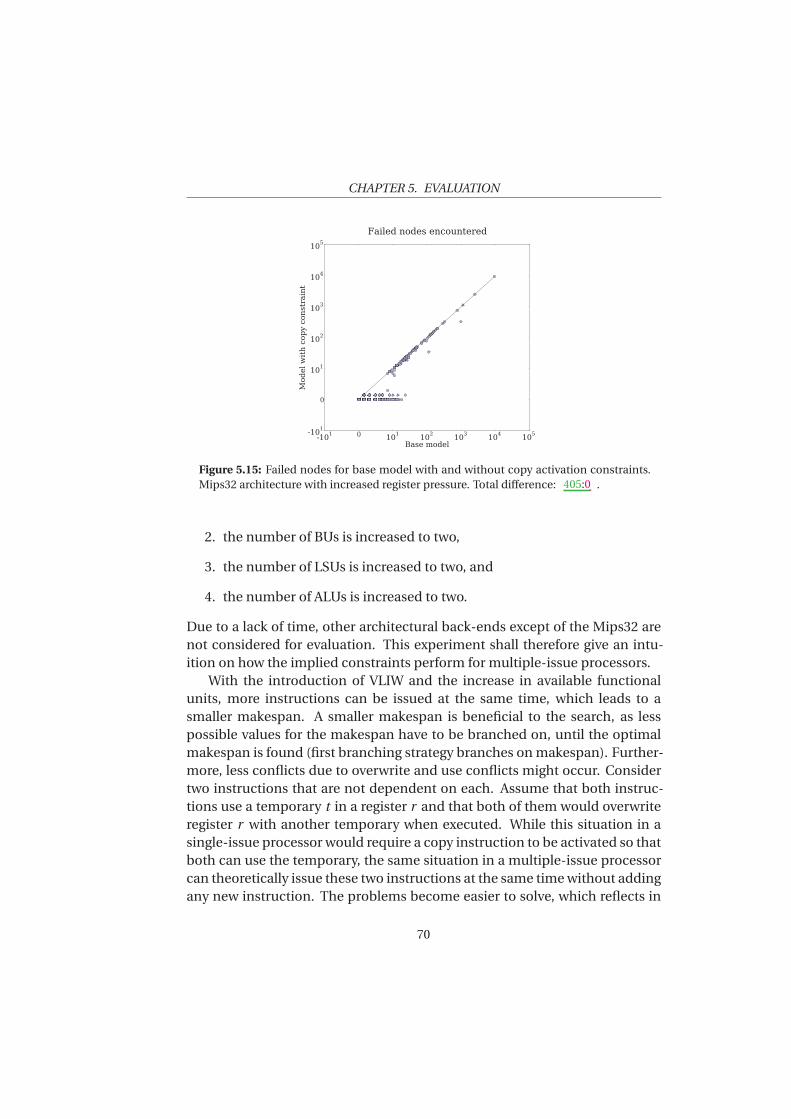
CHAPTER 5. EVALUATION
-10
1
0
10
1
10
2
10
3
10
4
10
5
Base model
-10
1
0
10
1
10
2
10
3
10
4
10
5
Model w
ith copy constraint
Failed nodes encountered
Figure 5.15: Failed nodes for base model with and without copy activation constraints.Mips32 architecture with increased register pressure. Total difference: 405:0 .
2. the number of BUs is increased to two,
3. the number of LSUs is increased to two, and
4. the number of ALUs is increased to two.
Due to a lack of time, other architectural back-ends except of the Mips32 arenot considered for evaluation. This experiment shall therefore give an intu-ition on how the implied constraints perform for multiple-issue processors.
With the introduction of VLIW and the increase in available functionalunits, more instructions can be issued at the same time, which leads to asmaller makespan. A smaller makespan is beneficial to the search, as lesspossible values for the makespan have to be branched on, until the optimalmakespan is found (first branching strategy branches on makespan). Further-more, less conflicts due to overwrite and use conflicts might occur. Considertwo instructions that are not dependent on each. Assume that both instruc-tions use a temporary t in a register r and that both of them would overwriteregister r with another temporary when executed. While this situation in asingle-issue processor would require a copy instruction to be activated so thatboth can use the temporary, the same situation in a multiple-issue processorcan theoretically issue these two instructions at the same time without addingany new instruction. The problems become easier to solve, which reflects in
70
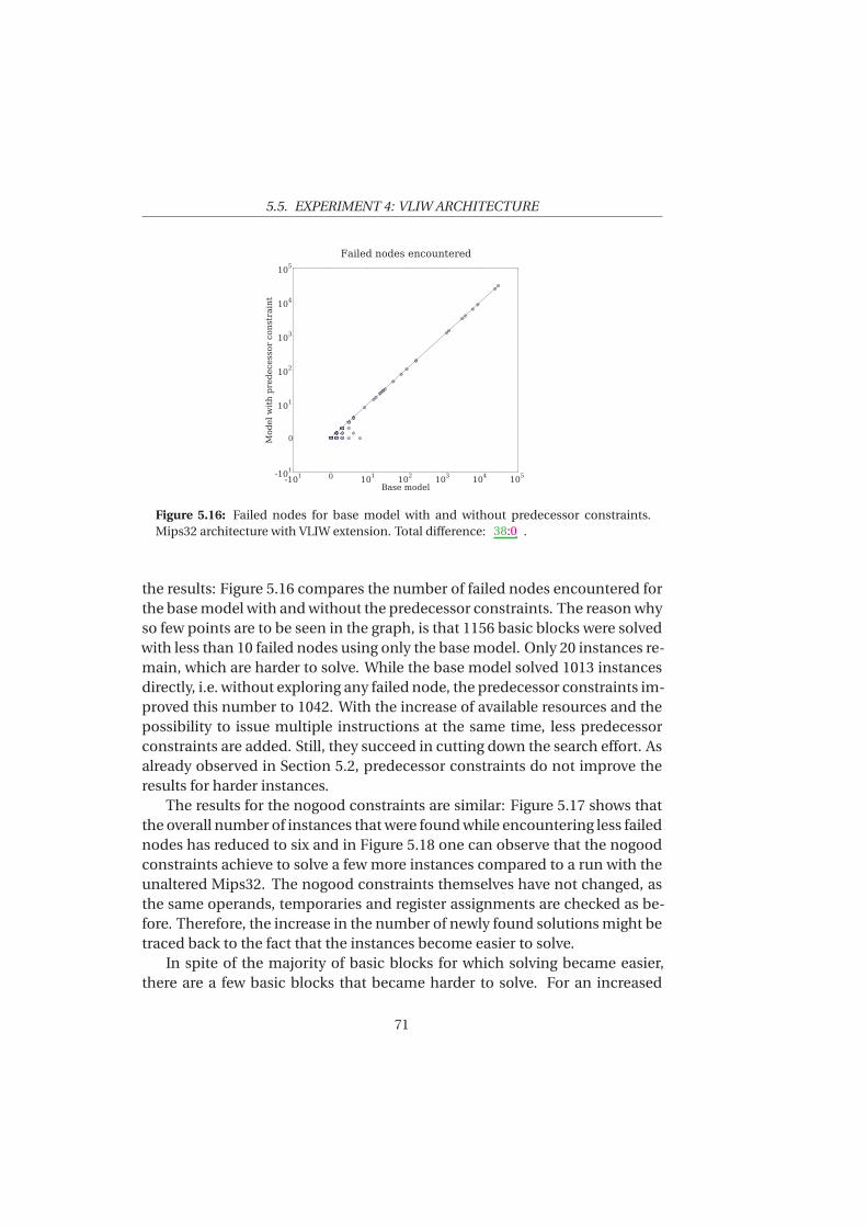
5.5. EXPERIMENT 4: VLIW ARCHITECTURE
-10
1
0
10
1
10
2
10
3
10
4
10
5
Base model
-10
1
0
10
1
10
2
10
3
10
4
10
5
Model w
ith predecessor constraint
Failed nodes encountered
Figure 5.16: Failed nodes for base model with and without predecessor constraints.Mips32 architecture with VLIW extension. Total difference: 38:0 .
the results: Figure 5.16 compares the number of failed nodes encountered forthe base model with and without the predecessor constraints. The reason whyso few points are to be seen in the graph, is that 1156 basic blocks were solvedwith less than 10 failed nodes using only the base model. Only 20 instances re-main, which are harder to solve. While the base model solved 1013 instancesdirectly, i.e. without exploring any failed node, the predecessor constraints im-proved this number to 1042. With the increase of available resources and thepossibility to issue multiple instructions at the same time, less predecessorconstraints are added. Still, they succeed in cutting down the search effort. Asalready observed in Section 5.2, predecessor constraints do not improve theresults for harder instances.
The results for the nogood constraints are similar: Figure 5.17 shows thatthe overall number of instances that were found while encountering less failednodes has reduced to six and in Figure 5.18 one can observe that the nogoodconstraints achieve to solve a few more instances compared to a run with theunaltered Mips32. The nogood constraints themselves have not changed, asthe same operands, temporaries and register assignments are checked as be-fore. Therefore, the increase in the number of newly found solutions might betraced back to the fact that the instances become easier to solve.
In spite of the majority of basic blocks for which solving became easier,there are a few basic blocks that became harder to solve. For an increased
71
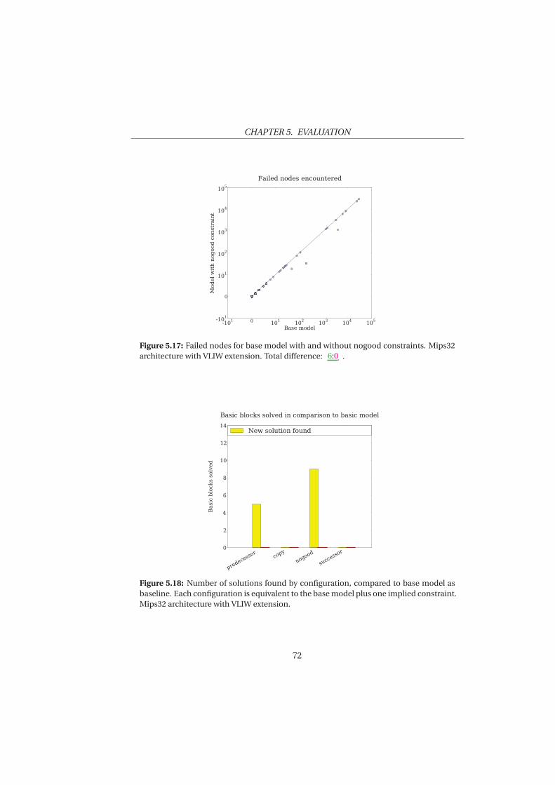
CHAPTER 5. EVALUATION
-10
1
0
10
1
10
2
10
3
10
4
10
5
Base model
-10
1
0
10
1
10
2
10
3
10
4
10
5
Model w
ith nogood constraint
Failed nodes encountered
Figure 5.17: Failed nodes for base model with and without nogood constraints. Mips32architecture with VLIW extension. Total difference: 6:0 .
p
r
e
d
e
c
e
s
s
o
r
c
o
p
y
n
o
g
o
o
d
s
u
c
c
e
s
s
o
r
0
2
4
6
8
10
12
14
Basic blocks solved
Basic blocks solved in comparison to basic model
New solution found
Figure 5.18: Number of solutions found by configuration, compared to base model asbaseline. Each configuration is equivalent to the base model plus one implied constraint.Mips32 architecture with VLIW extension.
72
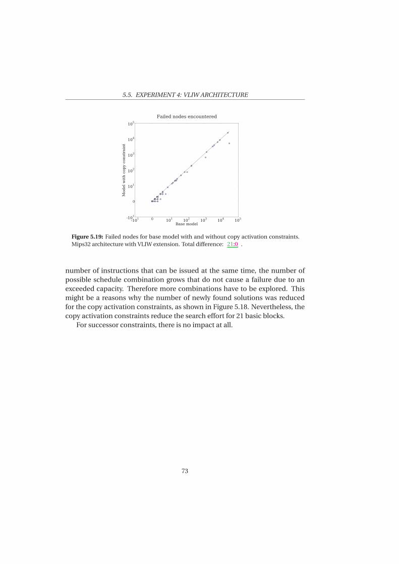
5.5. EXPERIMENT 4: VLIW ARCHITECTURE
-10
1
0
10
1
10
2
10
3
10
4
10
5
Base model
-10
1
0
10
1
10
2
10
3
10
4
10
5
Model w
ith copy constraint
Failed nodes encountered
Figure 5.19: Failed nodes for base model with and without copy activation constraints.Mips32 architecture with VLIW extension. Total difference: 21:0 .
number of instructions that can be issued at the same time, the number ofpossible schedule combination grows that do not cause a failure due to anexceeded capacity. Therefore more combinations have to be explored. Thismight be a reasons why the number of newly found solutions was reducedfor the copy activation constraints, as shown in Figure 5.18. Nevertheless, thecopy activation constraints reduce the search effort for 21 basic blocks.
For successor constraints, there is no impact at all.
73

CH
AP
TE
R
6DISCUSSION
This chapter picks up the leading questions from Chapter 5 and discussesthem on the basis of the results gained from the experimental runs.
If applicable, how do the implied constraints help to cut down the search
effort? In general, all implied constraints except of the successor constraintssucceeded in cutting down the search effort.
The predecessor constraints prune values from the lower bound of the is-sue cycle domains of instructions, which triggers further propagation throughother constraints that are defined in the base model. By the increased reduc-tion of the issue cycle domains, conflicts can be detected. Especially becausethe lower bound of the issue cycle of the out-delimiter is indirectly pruned,infeasible values for the makespan can be avoided to be branched on.
Similar to the predecessor constraints, the minimum makespan constraintsthat are part of the copy activation constraints reduced a lot of failed nodes bypruning the lower bound of the out-delimiter’s issue cycle. Furthermore, theharder instances could be solved by enforcing a number of mandatory instruc-tions to be active. For those cases where mandatory copies were introduced,the addition of copy activation constraints mostly led to a fast recognitionof infeasible assignments. Copy activation constraints helped to reduce thenumber of failed nodes for easy and medium hard problem instances.
Nogood constraints affected only a handful instances. These however, werepart of the hard problems to solve. By adding nogood constraints, infeasibleoperand-temporary assignments were reduced. The combination of the sec-ond branching strategy, which branches on the activity of an instruction, andthe reduction of the operand-temporary assignments led to the activation of
74
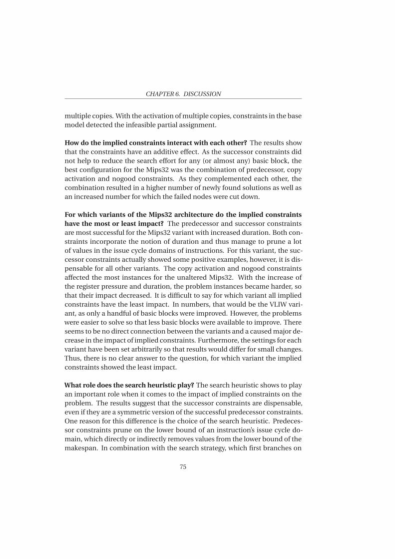
CHAPTER 6. DISCUSSION
multiple copies. With the activation of multiple copies, constraints in the basemodel detected the infeasible partial assignment.
How do the implied constraints interact with each other? The results showthat the constraints have an additive effect. As the successor constraints didnot help to reduce the search effort for any (or almost any) basic block, thebest configuration for the Mips32 was the combination of predecessor, copyactivation and nogood constraints. As they complemented each other, thecombination resulted in a higher number of newly found solutions as well asan increased number for which the failed nodes were cut down.
For which variants of the Mips32 architecture do the implied constraints
have the most or least impact? The predecessor and successor constraintsare most successful for the Mips32 variant with increased duration. Both con-straints incorporate the notion of duration and thus manage to prune a lotof values in the issue cycle domains of instructions. For this variant, the suc-cessor constraints actually showed some positive examples, however, it is dis-pensable for all other variants. The copy activation and nogood constraintsaffected the most instances for the unaltered Mips32. With the increase ofthe register pressure and duration, the problem instances became harder, sothat their impact decreased. It is difficult to say for which variant all impliedconstraints have the least impact. In numbers, that would be the VLIW vari-ant, as only a handful of basic blocks were improved. However, the problemswere easier to solve so that less basic blocks were available to improve. Thereseems to be no direct connection between the variants and a caused major de-crease in the impact of implied constraints. Furthermore, the settings for eachvariant have been set arbitrarily so that results would differ for small changes.Thus, there is no clear answer to the question, for which variant the impliedconstraints showed the least impact.
What role does the search heuristic play? The search heuristic shows to playan important role when it comes to the impact of implied constraints on theproblem. The results suggest that the successor constraints are dispensable,even if they are a symmetric version of the successful predecessor constraints.One reason for this difference is the choice of the search heuristic. Predeces-sor constraints prune on the lower bound of an instruction’s issue cycle do-main, which directly or indirectly removes values from the lower bound of themakespan. In combination with the search strategy, which first branches on
75
CHAPTER 6. DISCUSSION
the makespan, a lot of unnecessarily explored partial assignments can there-fore be avoided. Successor constraints, however, prune values of the upperbound of instructions and thus do not have the same impact as predecessorconstraints.
76
CH
AP
TE
R
7CONCLUSION AND FUTURE WORK
This chapter summarizes the results and gives an outlook on future work.
7.1 Results
The thesis investigated, presented and evaluated a set of implied constraintsaddressing register allocation and instruction scheduling. The results showthat the predecessor, copy activation and nogood constraints could success-fully reduce the search effort for all variants of the Mips32 architecture andeven for the adapted multiple-issue Mips32 processor. The impact of thepredecessor constraints especially increased with higher operation durations.Even if the instances became harder for some variants of the Mips32, each ofthem still achieved to avoid unnecessarily explored failed nodes. The nogoodconstraints only affected some basic blocks compared to the other two, butthose that were improved belong to the harder to solve basic blocks. As thenamed implied constraints complement each other, the best results could begained by combining them. Successor constraints, however, turn out to bedispensable for the given search heuristic. Therefore, a more accurate wayof finding implied constraints would have been to take the search heuristicinto consideration. The almost non existing impact of successor constraintsstresses the importance of the evaluation of implied constraints.
77
CHAPTER 7. CONCLUSION AND FUTURE WORK
7.2 Future Work
Apart from the predecessor and successor constraints, Malik et al. ([18]) presentseveral more implied constraints addressing instruction scheduling that canbe used for this model. For their scheduler, this model refinement was a keystep towards solving larger problems.
The implied constraints that are included into the base model in the scopeof this thesis were motivated by existing literature. Another way of findingimplied constraints is to follow a bottom-up approach [21]: finding impliedconstraints by analyzing the search tree. By looking at the search tree, onecan detect infeasible assignments that lead to infeasible partial search trees(contain only failed nodes). Ideally, an infeasible solution would directly bedetected as a dead-end. But as the solver continues to explore some of thesedead-ends, constraints are missing that would otherwise prevent it from ex-ploring them. The bottom up-approach might even produce more powerfulconstraints: if an implied constraint could be found using this approach, it isalready known to cut down the search effort for (at least) the specific instancethat was analyzed.
As mentioned in Chapter 6, the drawback on successor constraints wasdue to the fact that the search heuristic was not considered during investi-gation. Hence, customizing the search heuristic for given constraints mightincrease the effectiveness of the investigated constraints.
Malik et al. [18] present a heuristic to decrease the number of predeces-sor (and successor constraints) that are added to the model. Their algorithmis based on a sorted list, whereas the predecessors are sorted by their lowerbound. As an attempt to achieve a similar effect, the heuristic within this the-sis sorts the list of predecessors according to the number of their respectivepredecessors (see Section 3.1.2). An alternative way of sorting the predeces-sors that might be a more accurate adaptation of the heuristic proposed in[18] is to sort them by the number of hops between the root instruction andthe predecessor in a dependency graph.
Moreover, the scope of implied constraints was bound to static constraints,i.e. no new information during search was considered for adding new con-straints. A dynamic implementation of the implied constraints presented inthis thesis could result in further improvement.
78

AP
PE
ND
IX
AFIGURES
79
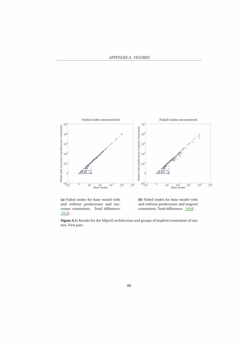
APPENDIX A. FIGURES
-10
1
0
10
1
10
2
10
3
10
4
10
5
Base model
-10
1
0
10
1
10
2
10
3
10
4
10
5
Model w
ith successor+
predecessor constraints
Failed nodes encountered
(a) Failed nodes for base model withand without predecessor and suc-cessor constraints. Total difference:292:0 .
-10
1
0
10
1
10
2
10
3
10
4
10
5
Base model
-10
1
0
10
1
10
2
10
3
10
4
10
5
Model w
ith predecessor+
nogood constraints
Failed nodes encountered
(b) Failed nodes for base model withand without predecessor and nogoodconstraints. Total difference: 309:0 .
Figure A.1: Results for the Mips32 architecture and groups of implied constraints of sizetwo. First part.
80
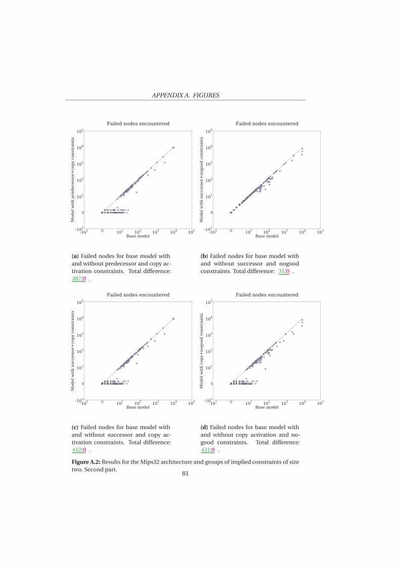
APPENDIX A. FIGURES
-10
1
0
10
1
10
2
10
3
10
4
10
5
Base model
-10
1
0
10
1
10
2
10
3
10
4
10
5
Model w
ith predecessor+
copy constraints
Failed nodes encountered
(a) Failed nodes for base model withand without predecessor and copy ac-tivation constraints. Total difference:487:0 .
-10
1
0
10
1
10
2
10
3
10
4
10
5
Base model
-10
1
0
10
1
10
2
10
3
10
4
10
5
Model w
ith successor+
nogood constraints
Failed nodes encountered
(b) Failed nodes for base model withand without successor and nogoodconstraints. Total difference: 31:0 .
-10
1
0
10
1
10
2
10
3
10
4
10
5
Base model
-10
1
0
10
1
10
2
10
3
10
4
10
5
Model w
ith successor+
copy constraints
Failed nodes encountered
(c) Failed nodes for base model withand without successor and copy ac-tivation constraints. Total difference:412:0 .
-10
1
0
10
1
10
2
10
3
10
4
10
5
Base model
-10
1
0
10
1
10
2
10
3
10
4
10
5
Model w
ith copy+
nogood constraints
Failed nodes encountered
(d) Failed nodes for base model withand without copy activation and no-good constraints. Total difference:431:0 .
Figure A.2: Results for the Mips32 architecture and groups of implied constraints of sizetwo. Second part.
81
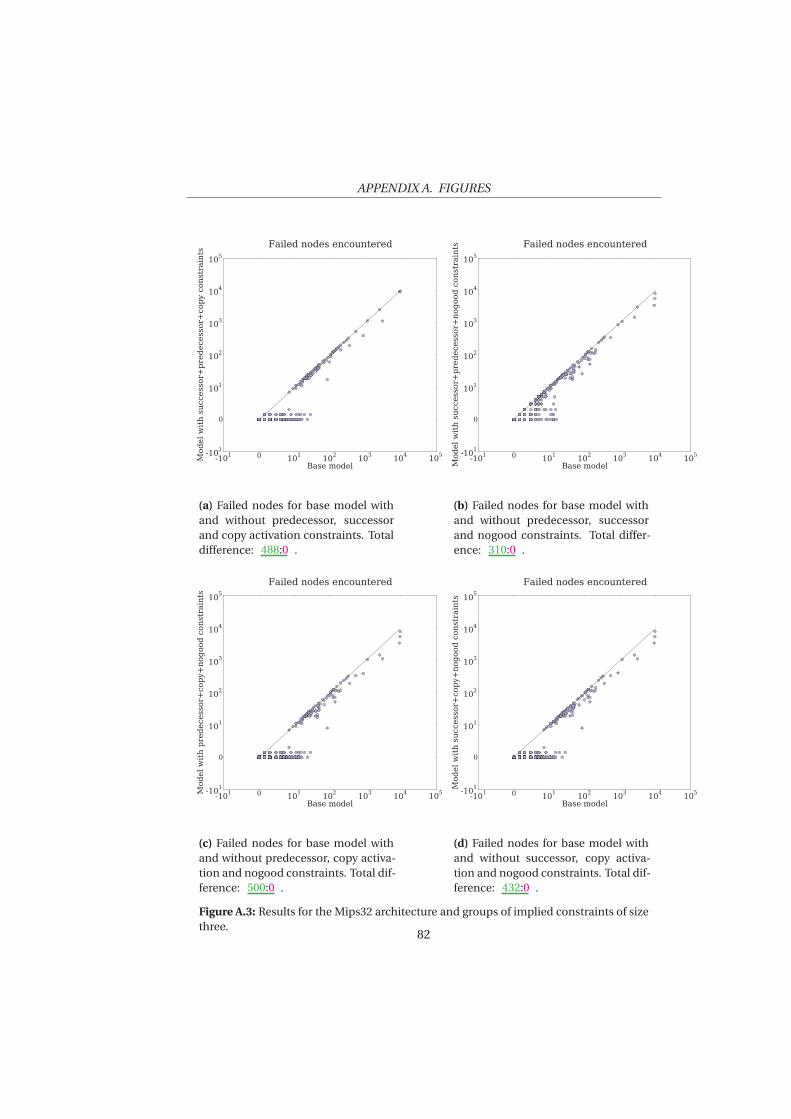
APPENDIX A. FIGURES
-10
1
0
10
1
10
2
10
3
10
4
10
5
Base model
-10
1
0
10
1
10
2
10
3
10
4
10
5
Model w
ith successor+
predecessor+
copy constraints
Failed nodes encountered
(a) Failed nodes for base model withand without predecessor, successorand copy activation constraints. Totaldifference: 488:0 .
-10
1
0
10
1
10
2
10
3
10
4
10
5
Base model
-10
1
0
10
1
10
2
10
3
10
4
10
5
Model with successor+predecessor+nogood constraints
Failed nodes encountered
(b) Failed nodes for base model withand without predecessor, successorand nogood constraints. Total differ-ence: 310:0 .
-10
1
0
10
1
10
2
10
3
10
4
10
5
Base model
-10
1
0
10
1
10
2
10
3
10
4
10
5
Model w
ith predecessor+
copy+
nogood constraints
Failed nodes encountered
(c) Failed nodes for base model withand without predecessor, copy activa-tion and nogood constraints. Total dif-ference: 500:0 .
-10
1
0
10
1
10
2
10
3
10
4
10
5
Base model
-10
1
0
10
1
10
2
10
3
10
4
10
5
Model w
ith successor+
copy+
nogood constraints
Failed nodes encountered
(d) Failed nodes for base model withand without successor, copy activa-tion and nogood constraints. Total dif-ference: 432:0 .
Figure A.3: Results for the Mips32 architecture and groups of implied constraints of sizethree.
82
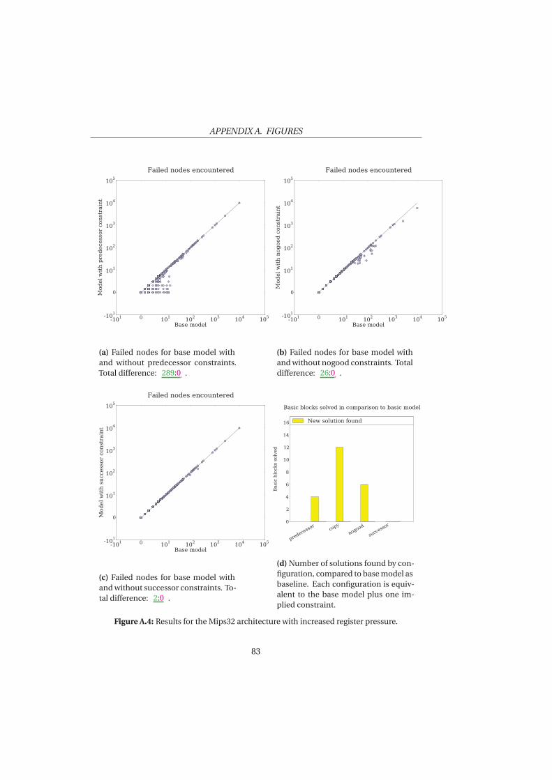
APPENDIX A. FIGURES
-10
1
0
10
1
10
2
10
3
10
4
10
5
Base model
-10
1
0
10
1
10
2
10
3
10
4
10
5
Model w
ith predecessor constraint
Failed nodes encountered
(a) Failed nodes for base model withand without predecessor constraints.Total difference: 289:0 .
-10
1
0
10
1
10
2
10
3
10
4
10
5
Base model
-10
1
0
10
1
10
2
10
3
10
4
10
5
Model w
ith nogood constraint
Failed nodes encountered
(b) Failed nodes for base model withand without nogood constraints. Totaldifference: 26:0 .
-10
1
0
10
1
10
2
10
3
10
4
10
5
Base model
-10
1
0
10
1
10
2
10
3
10
4
10
5
Model w
ith successor constraint
Failed nodes encountered
(c) Failed nodes for base model withand without successor constraints. To-tal difference: 2:0 .
p
r
e
d
e
c
e
s
s
o
r
c
o
p
y
n
o
g
o
o
d
s
u
c
c
e
s
s
o
r
0
2
4
6
8
10
12
14
16
Basic blocks solved
Basic blocks solved in comparison to basic model
New solution found
(d) Number of solutions found by con-figuration, compared to base model asbaseline. Each configuration is equiv-alent to the base model plus one im-plied constraint.
Figure A.4: Results for the Mips32 architecture with increased register pressure.
83
AP
PE
ND
IX
BCONSTRAINT MODEL
B.1 Constraint Model
The model is reprinted from [15].
84
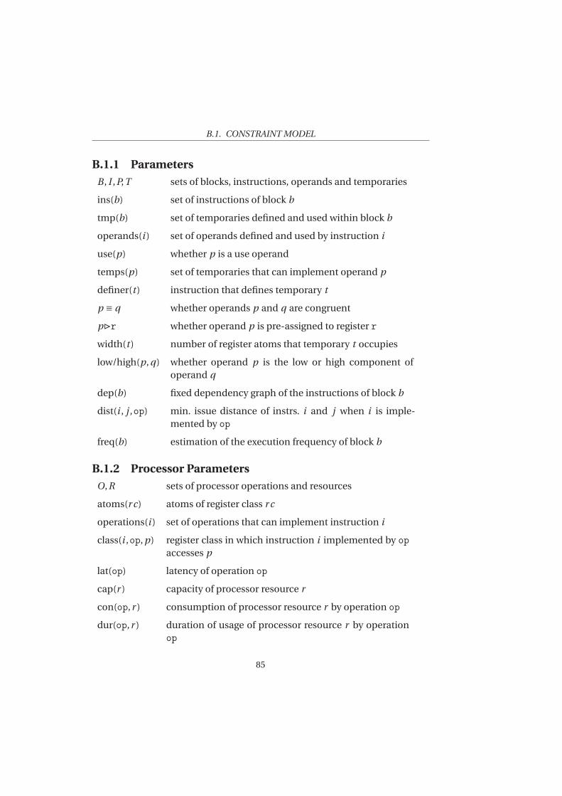
B.1. CONSTRAINT MODEL
B.1.1 Parameters
B , I ,P,T sets of blocks, instructions, operands and temporaries
ins(b) set of instructions of block b
tmp(b) set of temporaries defined and used within block b
operands(i ) set of operands defined and used by instruction i
use(p) whether p is a use operand
temps(p) set of temporaries that can implement operand p
definer(t ) instruction that defines temporary t
p ≡ q whether operands p and q are congruent
p⊲r whether operand p is pre-assigned to register r
width(t ) number of register atoms that temporary t occupies
low/high(p, q) whether operand p is the low or high component ofoperand q
dep(b) fixed dependency graph of the instructions of block b
dist(i , j ,op) min. issue distance of instrs. i and j when i is imple-mented by op
freq(b) estimation of the execution frequency of block b
B.1.2 Processor Parameters
O,R sets of processor operations and resources
atoms(r c) atoms of register class r c
operations(i ) set of operations that can implement instruction i
class(i ,op, p) register class in which instruction i implemented by op
accesses p
lat(op) latency of operation op
cap(r ) capacity of processor resource r
con(op,r ) consumption of processor resource r by operation op
dur(op,r ) duration of usage of processor resource r by operationop
85
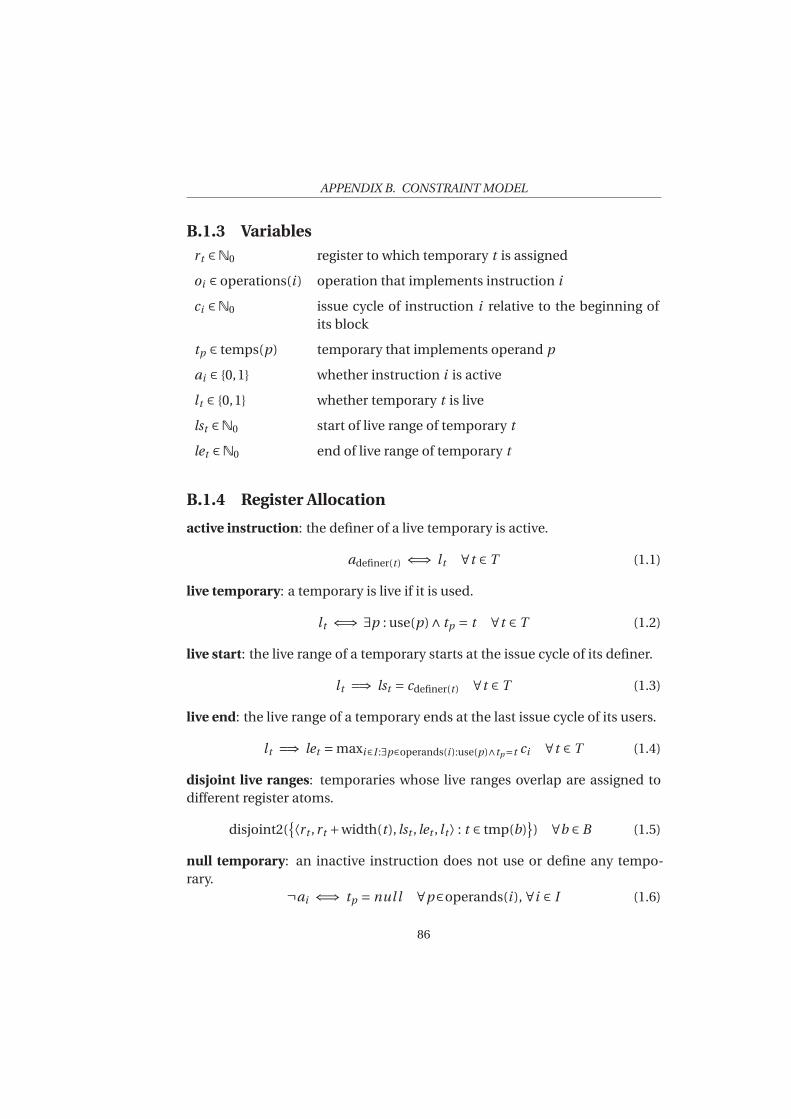
APPENDIX B. CONSTRAINT MODEL
B.1.3 Variables
rt ∈N0 register to which temporary t is assigned
oi ∈ operations(i ) operation that implements instruction i
ci ∈N0 issue cycle of instruction i relative to the beginning ofits block
tp ∈ temps(p) temporary that implements operand p
ai ∈ {0,1} whether instruction i is active
lt ∈ {0,1} whether temporary t is live
lst ∈N0 start of live range of temporary t
let ∈N0 end of live range of temporary t
B.1.4 Register Allocation
active instruction: the definer of a live temporary is active.
adefiner(t ) ⇐⇒ lt ∀t ∈ T (1.1)
live temporary: a temporary is live if it is used.
lt ⇐⇒ ∃p : use(p)∧ tp = t ∀t ∈ T (1.2)
live start: the live range of a temporary starts at the issue cycle of its definer.
lt =⇒ lst = cdefiner(t ) ∀t ∈ T (1.3)
live end: the live range of a temporary ends at the last issue cycle of its users.
lt =⇒ let = maxi∈I :∃p∈operands(i ):use(p)∧tp=t ci ∀t ∈ T (1.4)
disjoint live ranges: temporaries whose live ranges overlap are assigned todifferent register atoms.
disjoint2({
⟨rt ,rt +width(t ), lst , let , lt ⟩ : t ∈ tmp(b)}
) ∀b ∈ B (1.5)
null temporary: an inactive instruction does not use or define any tempo-rary.
¬ai ⇐⇒ tp = null ∀p∈operands(i ), ∀i ∈ I (1.6)
86
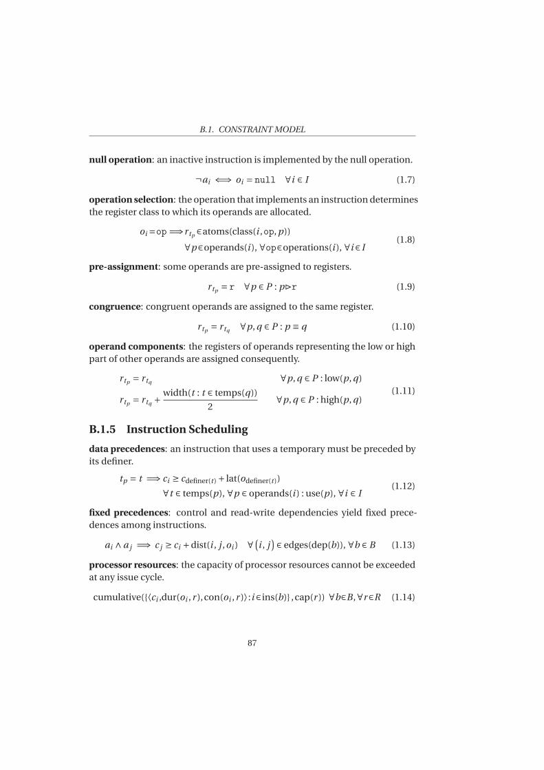
B.1. CONSTRAINT MODEL
null operation: an inactive instruction is implemented by the null operation.
¬ai ⇐⇒ oi = null ∀i ∈ I (1.7)
operation selection: the operation that implements an instruction determinesthe register class to which its operands are allocated.
oi =op =⇒rtp ∈atoms(class(i ,op, p))
∀p∈operands(i ), ∀op∈operations(i ), ∀i∈I(1.8)
pre-assignment: some operands are pre-assigned to registers.
rtp = r ∀p ∈ P : p⊲r (1.9)
congruence: congruent operands are assigned to the same register.
rtp = rtq ∀p, q ∈ P : p ≡ q (1.10)
operand components: the registers of operands representing the low or highpart of other operands are assigned consequently.
rtp = rtq ∀p, q ∈ P : low(p, q)
rtp = rtq +width(t : t ∈ temps(q))
2∀p, q ∈ P : high(p, q)
(1.11)
B.1.5 Instruction Scheduling
data precedences: an instruction that uses a temporary must be preceded byits definer.
tp = t =⇒ ci ≥ cdefiner(t ) + lat(odefiner(t ))
∀t ∈ temps(p), ∀p ∈ operands(i ) : use(p), ∀i ∈ I(1.12)
fixed precedences: control and read-write dependencies yield fixed prece-dences among instructions.
ai ∧a j =⇒ c j ≥ ci +dist(i , j ,oi ) ∀(
i , j)
∈ edges(dep(b)), ∀b ∈ B (1.13)
processor resources: the capacity of processor resources cannot be exceededat any issue cycle.
cumulative({⟨ci ,dur(oi ,r ),con(oi ,r )⟩:i∈ins(b)} ,cap(r )) ∀b∈B ,∀r∈R (1.14)
87
BIBLIOGRAPHY
[1] Alfred V. Aho, Monica S. Lam, Ravi Sethi, and Jeffrey D. Ullman. Com-
pilers: Principles, Techniques, and Tools (2nd Edition). Addison-WesleyLongman Publishing Co., Inc., Boston, MA, USA, 2006.
[2] Andrzej Bednarski and Christoph W. Kessler. Optimal integrated VLIWcode generation with integer linear programming. In Wolfgang E. Nagel,Wolfgang V. Walter, and Wolfgang Lehner, editors, Euro-Par 2006 Parallel
Processing: 12th International Euro-Par Conference, volume 4128 of Lec-
ture Notes in Computer Science, pages 461–472. Springer-Verlag, 2006.
[3] Mats Carlsson. Nogood generation using SAT and the definition of valueconsistency. Personal communication. June, 2013.
[4] Gregory J. Chaitin. Register allocation & spilling via graph coloring. InJohn R. White and Frances E. Allen, editors, Proceedings of the SIGPLAN
’82 Symposium on Compiler Construction, pages 98–105, 1982.
[5] Geoffrey Chu and Peter J. Stuckey. A generic method for identifying andexploiting dominance relations. In Michela Milano, editor, Eighteenth In-
ternational Conference on Principles and Practice of Constraint Program-
ming, volume 7514 of Lecture Notes in Computer Science, pages 6–22.Springer-Verlag, 2012.
[6] Open Data Commons. Open data commons attribution license.http://opendatacommons.org/licenses/by/1.0/. Accessed July 24, 2013.
[7] Stephen A. Cook. The complexity of theorem-proving procedures. InMichael A. Harrison, Ranan B. Banerji, and Jeffrey D. Ullman, editors,Proceedings of the third annual ACM Symposium on Theory of Comput-
ing, STOC ’71, pages 151–158. ACM, 1971.
[8] Rina Dechter. Learning while searching in constraint-satisfaction-problems. In Tom Kehler, editor, Proceedings of the Fifth National Con-
ference on Artificial Intelligence, volume 1, pages 178–185. Morgan Kauf-mann, 1986.
88
B.1. CONSTRAINT MODEL
[9] M. Anton Ertl and Andreas Krall. Optimal instruction scheduling usingconstraint logic programming. In Jan Maluszynski and Martin Wirsing,editors, Programming Language Implementation and Logic Program-
ming, volume 528 of Lecture Notes in Computer Science, pages 75–86.Springer-Verlag, 1991.
[10] Martin Erwig and Ivan L. Miljenovic. Functional graph library.http://hackage.haskell.org/package/fgl-5.4.2.4. Accessed July 27, 2013.
[11] Alan M. Frisch, Christopher Jefferson, and Ian Miguel. Symmetry break-ing as a prelude to implied constraints: A constraint modelling pattern.In Ramón López de Mántaras and Lorenza Saitta, editors, Proceedings
of the 16th European Conference on Artificial Intelligence, pages 171–175.IOS Press, 2004.
[12] David W. Goodwin and Kent D. Wilken. Optimal and near-optimal globalregister allocation using 0-1 integer programming. Software – Practice
and Experience, 26(8):929–965, August 1996.
[13] John L. Henning. Spec cpu2006 benchmark descriptions. SIGARCH Com-
puter Architecture News, 34(4):1–17, September 2006.
[14] John D. Hunter. Matplotlib: A 2d graphics environment. Computing In
Science & Engineering, 9(3):90–95, 2007.
[15] Roberto Castañeda Lozano and Mats Carlsson. Constraint-based registerallocation and instruction scheduling. This document complements theCP2012 paper with design notes and implementation details. AccessedMarch 15, 2013.
[16] Roberto Castañeda Lozano, Mats Carlsson, Frej Drejhammar, and Chris-tian Schulte. Constraint-based register allocation and instructionscheduling. In Michela Milano, editor, Eighteenth International Confer-
ence on Principles and Practice of Constraint Programming, volume 7514of Lecture Notes in Computer Science, pages 750–766. Springer-Verlag,2012.
[17] Abid M. Malik. Constraint Programming Techniques for Optimal Instruc-
tion Scheduling. PhD thesis, University of Waterloo, 2008.
89
APPENDIX B. CONSTRAINT MODEL
[18] Abid M. Malik, Jim McInnes, and Peter van Beek. Optimal basic block in-struction scheduling for multiple-issue processors using constraint pro-gramming. International Journal on Artificial Intelligence Tools, 17(1):37–54, February 2008.
[19] João Marques-Silva. Practical applications of Boolean satisfiability. InBengt Lennartson, Martin Fabian, Knut Åkesson, Alessandro Giua, andRatnesh Kumar, editors, WODES’08: Proceedings of the 9th International
Workshop on Discrete Event Systems, pages 74–80. IEEE Press, 2008.
[20] Inc. MIPS Technologies. MIPS32™ architecture for programmers vol-ume i: Introduction to the MIPS32™ architecture. Technical ReportMD00082, 2001.
[21] Barbara M. Smith. Modelling. In Francesca Rossi, Peter Van Beek, andToby Walsh, editors, Handbook of Constraint Programming, chapter 11,pages 377–406. Elsevier Science Inc., New York, NY, USA, 2006.
[22] Niklas Sörensson. MiniSat 2.2 and MiniSat++ 1.1.http://baldur.iti.uka.de/sat-race-2010/descriptions/solver_25+26.pdf,2010. Accessed July 16, 2013.
[23] Niklas Sörensson and Niklas Eén. MiniSat: A minimalistic, open-sourceSAT solver. http://minisat.se/. Accessed July 16, 2013.
[24] DBLP Team. The DBLP computer science bibliography.http://www.informatik.uni-trier.de/~ley/db/. Accessed July 16, 2013.
[25] Gecode Team. Gecode: Generic constraint development environment.http://www.gecode.org/. Accessed June 24, 2013.
[26] Peter van Beek. Backtracking search algorithms. In Francesca Rossi, Pe-ter Van Beek, and Toby Walsh, editors, Handbook of Constraint Program-
ming, chapter 4, pages 85–134. Elsevier Science Inc., New York, NY, USA,2006.
[27] Kent D. Wilken, Jack Liu, and Mark Heffernan. Optimal instructionscheduling using integer programming. In Monica S. Lam, editor, Pro-
ceedings of the ACM SIGPLAN 2000 conference on Programming language
design and implementation, pages 121–133. ACM, 2000.
90