Embed Size (px)
Citation preview
Nearest Neighbor Searchin High-Dimensional Spaces
Alexandr Andoni(Microsoft Research Silicon Valley)
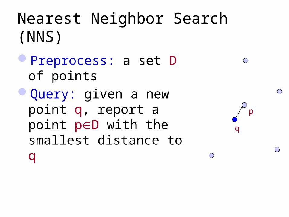
Nearest Neighbor Search (NNS)
Preprocess: a set D of points
Query: given a new point q, report a point pD with the smallest distance to q q
p
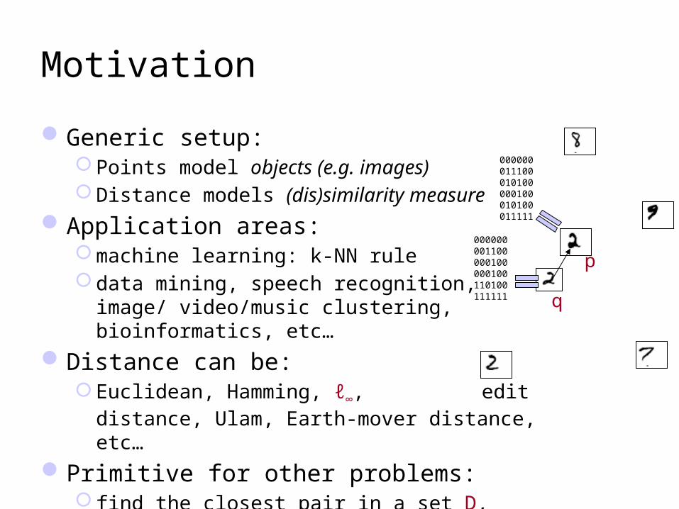
Motivation
Generic setup: Points model objects (e.g. images) Distance models (dis)similarity measure
Application areas: machine learning: k-NN rule data mining, speech recognition, image/
video/music clustering, bioinformatics, etc…
Distance can be: Euclidean, Hamming, ℓ∞, edit
distance, Ulam, Earth-mover distance, etc…
Primitive for other problems: find the closest pair in a set D, MST, clustering…
q
p
000000011100010100000100010100011111
000000001100000100000100110100111111
Further motivation?
4
eHarmony: 29 Dimensions® of Compatibily
Plan for today
1. NNS for basic distances
2. NNS for advanced distances: reductions
3. NNS via composition
Plan for today
1. NNS for basic distances
2. NNS for advanced distances: reductions
3. NNS via composition
7
Euclidean distance
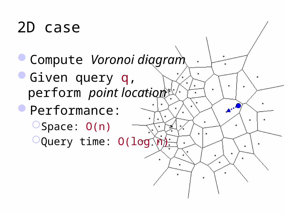
2D case
Compute Voronoi diagramGiven query q, perform
point locationPerformance:
Space: O(n)Query time: O(log n)
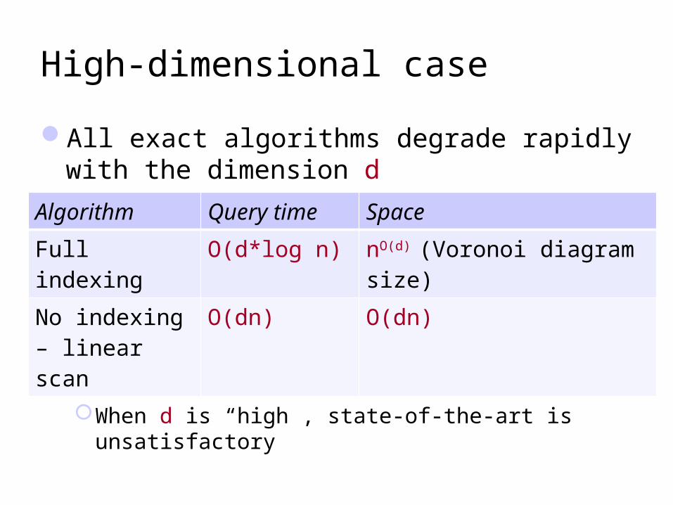
High-dimensional case
All exact algorithms degrade rapidly with the dimension d
In practice:When d is “medium”, kd-trees work betterWhen d is “high”, state-of-the-art is unsatisfactory
Algorithm Query time Space
Full indexing O(d*log n) nO(d) (Voronoi diagram size)
No indexing – linear scan
O(dn) O(dn)
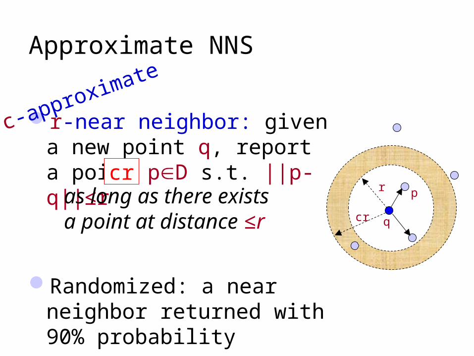
Approximate NNS
r-near neighbor: given a new point q, report a point pD s.t. ||p-q||≤r
Randomized: a near neighbor returned with 90% probability
c-approximate
cras long as there existsa point at distance ≤r q
r p
cr
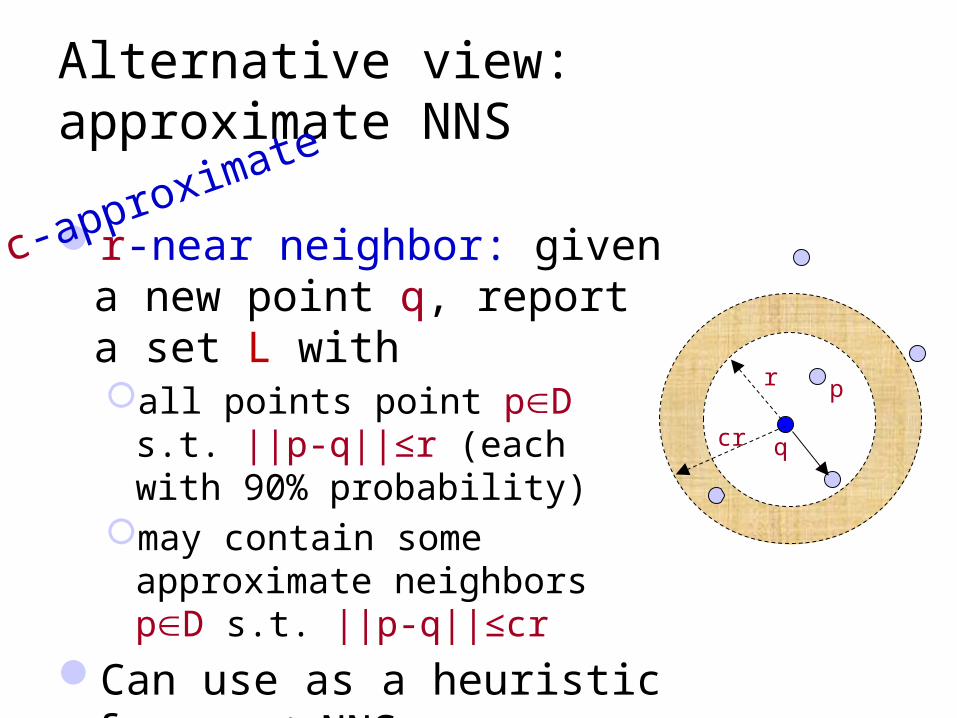
Alternative view: approximate NNS
r-near neighbor: given a new point q, report a set L withall points point pD s.t. ||p-q||≤r
(each with 90% probability)may contain some approximate
neighbors pD s.t. ||p-q||≤cr
Can use as a heuristic for exact NNS
c-approximate
q
r p
cr
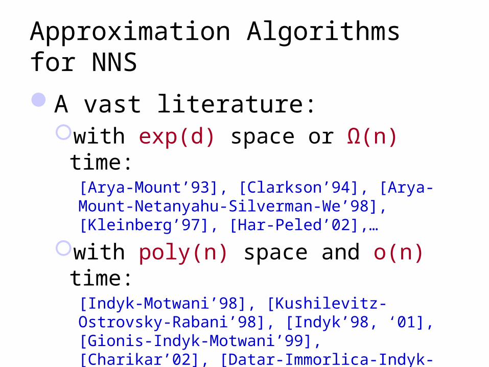
Approximation Algorithms for NNS
A vast literature:with exp(d) space or Ω(n) time:
[Arya-Mount’93], [Clarkson’94], [Arya-Mount-Netanyahu-Silverman-We’98], [Kleinberg’97], [Har-Peled’02],…
with poly(n) space and o(n) time: [Indyk-Motwani’98], [Kushilevitz-Ostrovsky-Rabani’98], [Indyk’98, ‘01], [Gionis-Indyk-Motwani’99], [Charikar’02], [Datar-Immorlica-Indyk-Mirrokni’04], [Chakrabarti-Regev’04], [Panigrahy’06], [Ailon-Chazelle’06], [A-Indyk’06]…
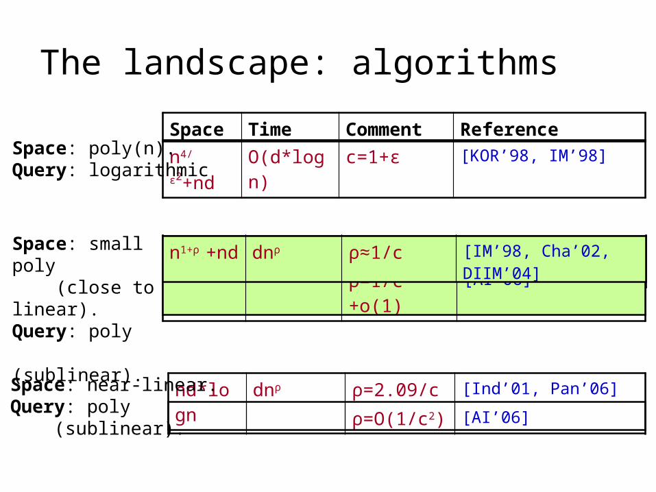
ρ=1/c2 +o(1) [AI’06]
n1+ρ +nd dnρ ρ≈1/c [IM’98, Cha’02, DIIM’04]
The landscape: algorithms
ρ=O(1/c2) [AI’06]
n4/ε2+nd O(d*log n) c=1+ε [KOR’98, IM’98]
nd*logn dnρ ρ=2.09/c [Ind’01, Pan’06]
Space: poly(n).Query: logarithmic
Space: small poly (close to linear). Query: poly (sublinear).
Space: near-linear.Query: poly (sublinear).
Space Time Comment Reference
ρ=1/c2 +o(1) [AI’06]
n1+ρ +nd dnρ ρ≈1/c [IM’98, Cha’02, DIIM’04]
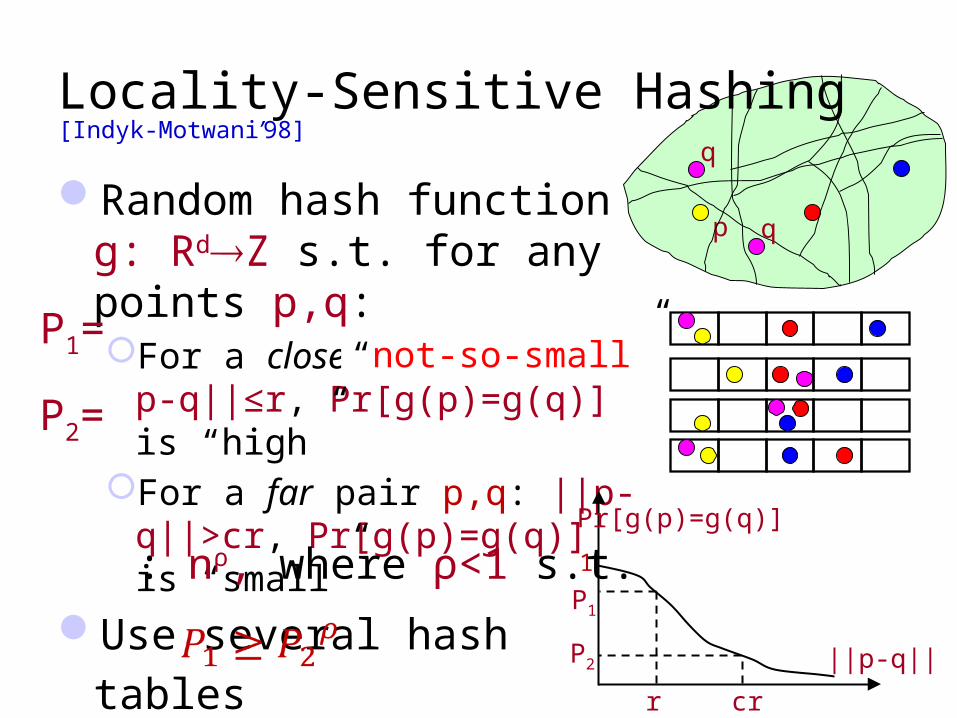
Locality-Sensitive Hashing
Random hash function g: RdZ s.t. for any points p,q:For a close pair p,q: ||p-q||≤r,
Pr[g(p)=g(q)] is “high” For a far pair p,q: ||p-q||>cr,
Pr[g(p)=g(q)] is “small”
Use several hash
tables
q
p
||p-q||
Pr[g(p)=g(q)]
r cr
1
P1
P2
: nρ, where ρ<1 s.t.
[Indyk-Motwani’98]
q
“not-so-small”
P1=
P2=
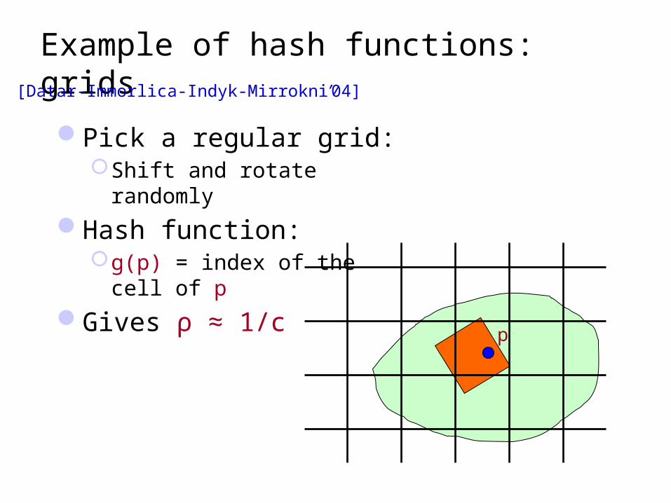
Example of hash functions: grids
Pick a regular grid:Shift and rotate randomly
Hash function:g(p) = index of the cell of p
Gives ρ ≈ 1/c
p
[Datar-Immorlica-Indyk-Mirrokni’04]
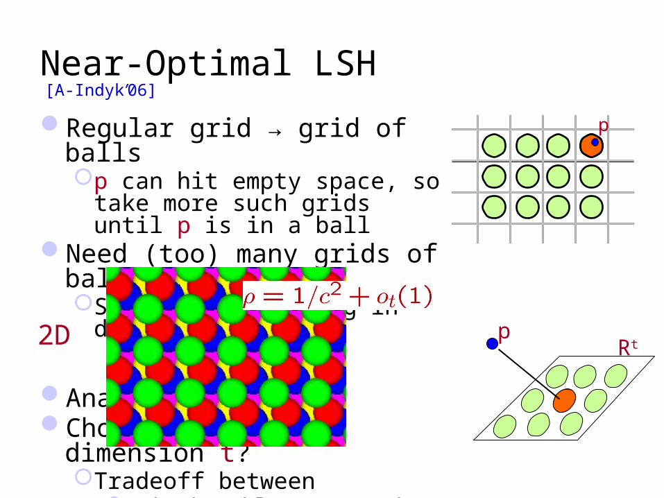
Regular grid → grid of ballsp can hit empty space, so take
more such grids until p is in a ballNeed (too) many grids of balls
Start by projecting in dimension t
Analysis givesChoice of reduced dimension t?
Tradeoff between
# hash tables, n, andTime to hash, tO(t)
Total query time: dn1/c2+o(1)
Near-Optimal LSH
2D
p
pRt
[A-Indyk’06]
x
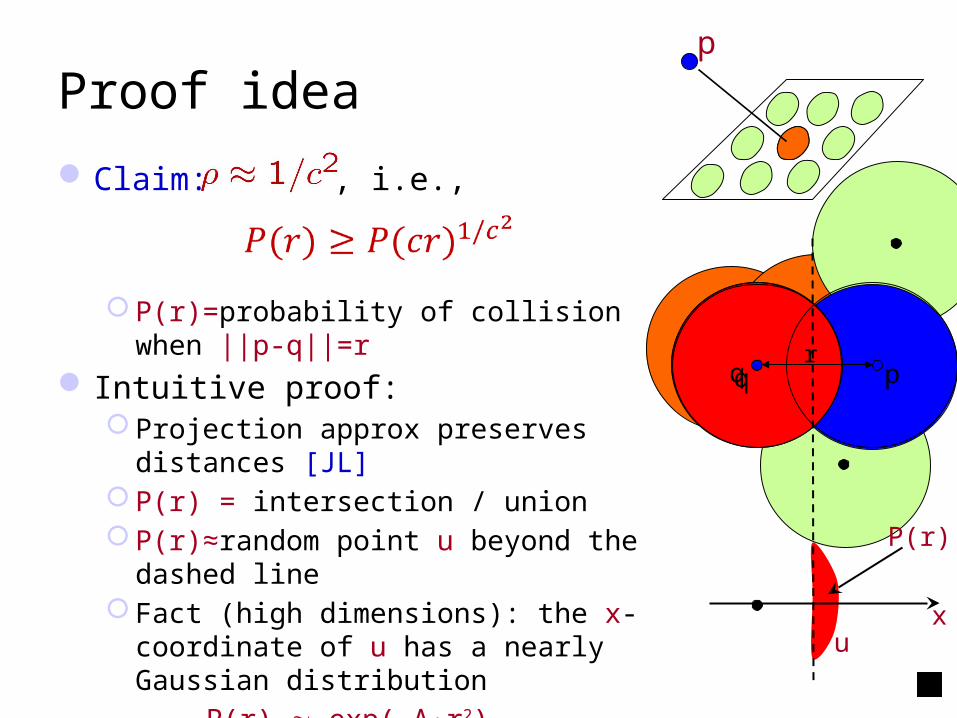
Proof idea
Claim: , i.e.,
P(r)=probability of collision when ||p-q||=r Intuitive proof:
Projection approx preserves distances [JL] P(r) = intersection / union P(r)≈random point u beyond the dashed line Fact (high dimensions): the x-coordinate of u
has a nearly Gaussian distribution
→ P(r) exp(-A·r2)
pqr
q
P(r)
u
p
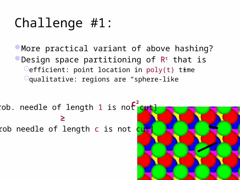
Challenge #1:
More practical variant of above hashing?Design space partitioning of Rt that is
efficient: point location in poly(t) timequalitative: regions are “sphere-like”
[Prob. needle of length 1 is not cut]
[Prob needle of length c is not cut]
≥
c2
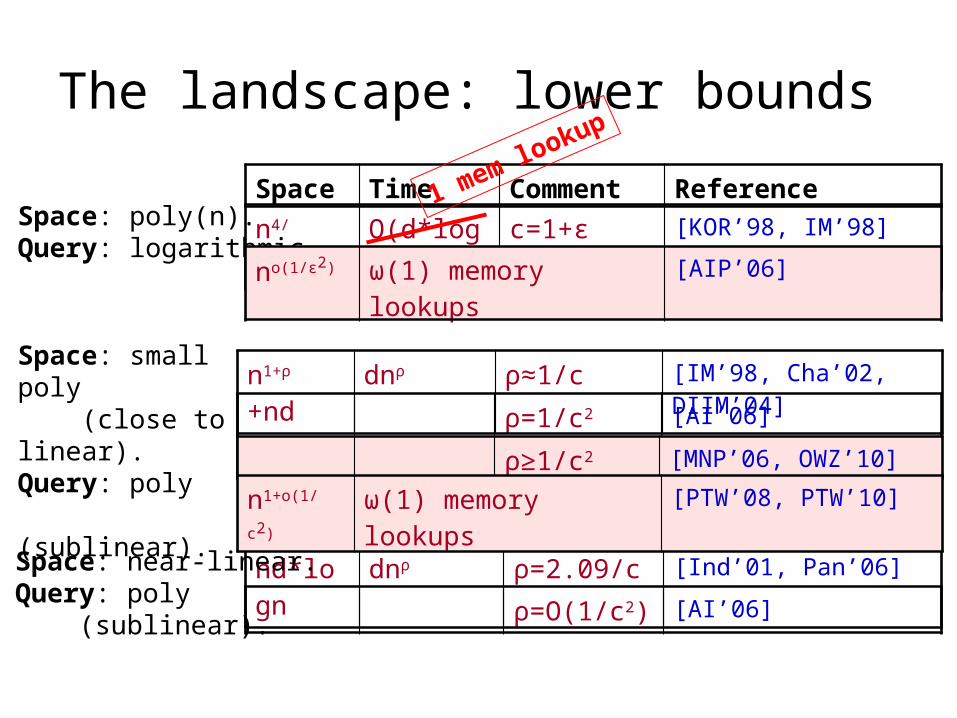
The landscape: lower bounds
ρ=1/c2 +o(1) [AI’06]
ρ=O(1/c2) [AI’06]
n4/ε2+nd O(d*log n) c=1+ε [KOR’98, IM’98]
n1+ρ +nd dnρ ρ≈1/c [IM’98, Cha’02, DIIM’04]
nd*logn dnρ ρ=2.09/c [Ind’01, Pan’06]
Space: poly(n).Query: logarithmic
Space: small poly (close to linear). Query: poly (sublinear).
Space: near-linear.Query: poly (sublinear).
Space Time Comment Reference
no(1/ε2) ω(1) memory lookups [AIP’06]
ρ≥1/c2 [MNP’06, OWZ’10]
n1+o(1/c2) ω(1) memory lookups [PTW’08, PTW’10]
1 mem lookup
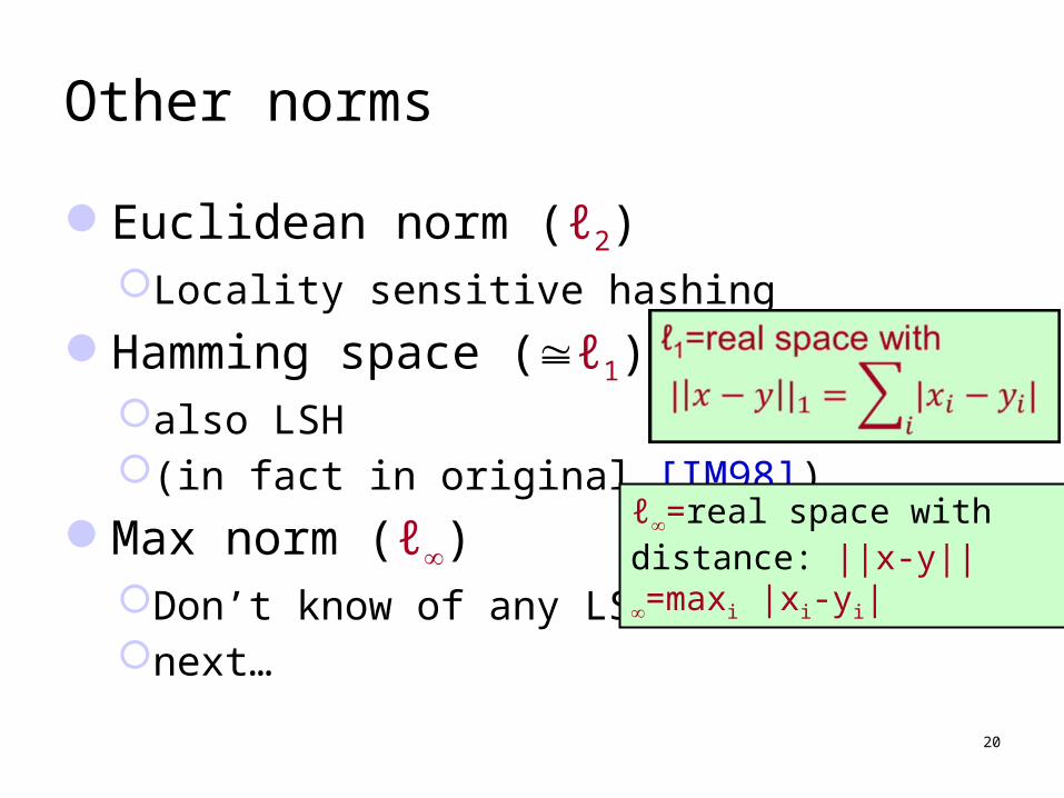
Other norms
Euclidean norm (ℓ2)Locality sensitive hashing
Hamming space (ℓ1)also LSH(in fact in original [IM98])
Max norm (ℓ)Don’t know of any LSHnext…
20
ℓ=real space with distance: ||x-y||=maxi |xi-yi|
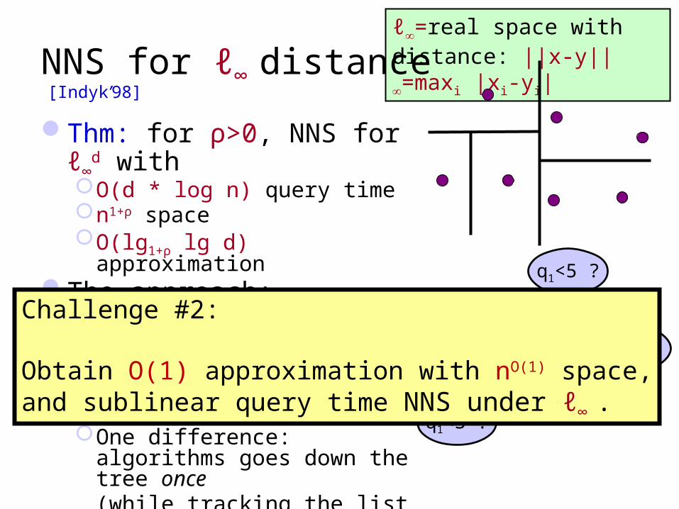
ℓ=real space with distance: ||x-y||=maxi |xi-yi|NNS for ℓ∞ distance
Thm: for ρ>0, NNS for ℓ∞d with
O(d * log n) query timen1+ρ spaceO(lg1+ρ lg d) approximation
The approach:A deterministic decision tree
Similar to kd-treesEach node of DT is “qi < t”One difference: algorithms goes
down the tree once(while tracking the list of possible neighbors)
[ACP’08]: optimal for deterministic decision trees!
q2<3 ?q2<4 ?
Yes No
q1<3 ?
Yes No
q1<5 ?
[Indyk’98]
Challenge #2:
Obtain O(1) approximation with nO(1) space,and sublinear query time NNS under ℓ∞ .
Plan for today
1. NNS for basic distances
2. NNS for advanced distances: reductions
3. NNS via composition
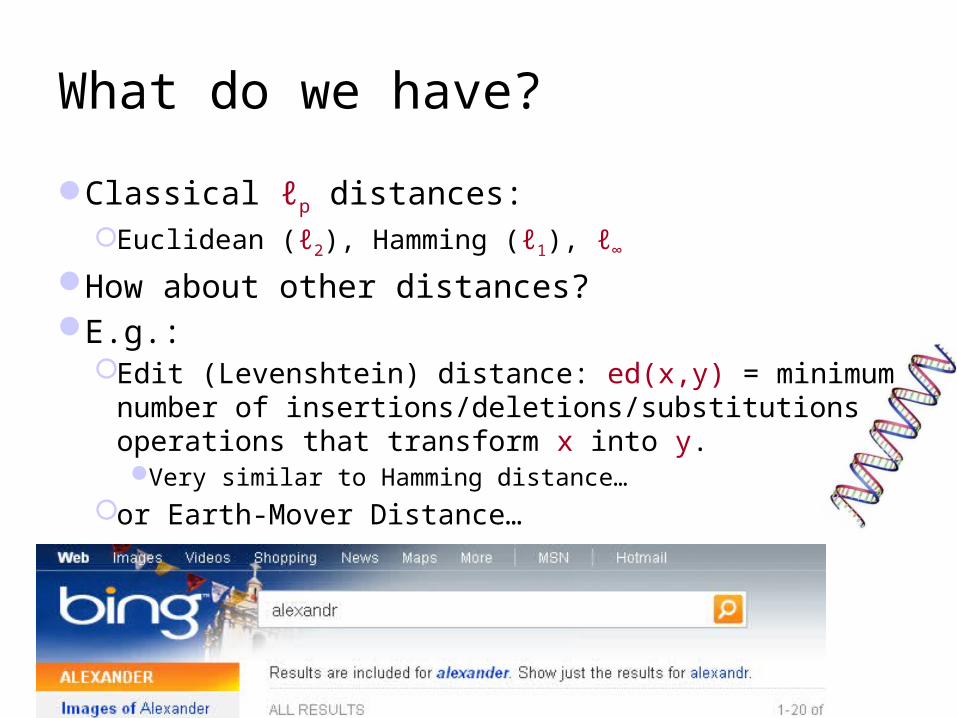
What do we have?
Classical ℓp distances:Euclidean (ℓ2), Hamming (ℓ1), ℓ∞
How about other distances?E.g.:
Edit (Levenshtein) distance: ed(x,y) = minimum number of insertions/deletions/substitutions operations that transform x into y.Very similar to Hamming distance…
or Earth-Mover Distance…
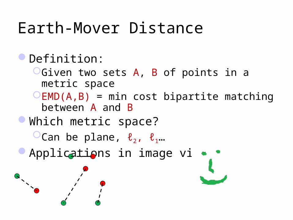
Earth-Mover Distance
Definition:Given two sets A, B of points in a metric spaceEMD(A,B) = min cost bipartite matching between A
and BWhich metric space?
Can be plane, ℓ2, ℓ1…Applications in image vision
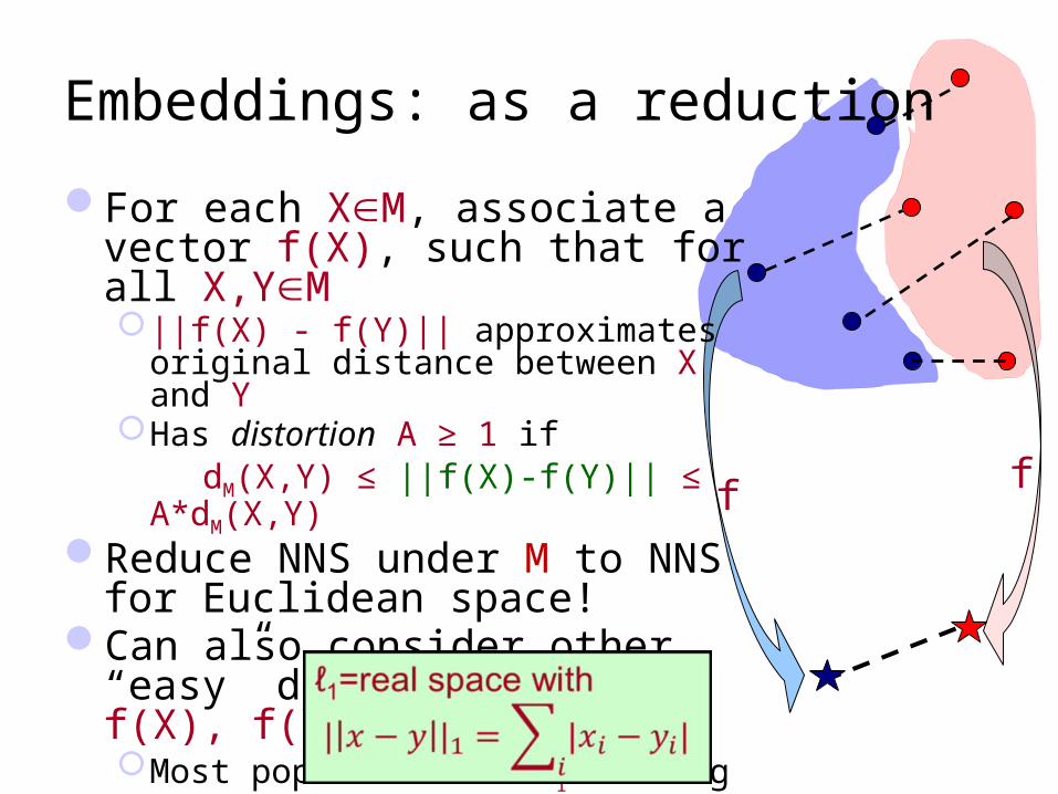
Embeddings: as a reduction
f
For each XM, associate a vector f(X), such that for all X,YM ||f(X) - f(Y)|| approximates original
distance between X and YHas distortion A ≥ 1 if
dM(X,Y) ≤ ||f(X)-f(Y)|| ≤ A*dM(X,Y)
Reduce NNS under M to NNS for Euclidean space!
Can also consider other “easy” distances between f(X), f(Y)Most popular host: ℓ1≡Hamming
f
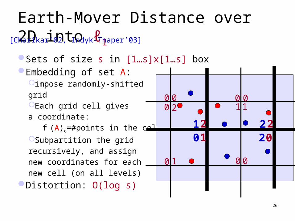
Earth-Mover Distance over 2D into ℓ1
Sets of size s in [1…s]x[1…s] boxEmbedding of set A:
impose randomly-shifted
grid Each grid cell gives
a coordinate:
f (A)c=#points in the cell c
Subpartition the grid
recursively, and assign
new coordinates for each
new cell (on all levels)
Distortion: O(log s)
26
[Charikar’02, Indyk-Thaper’03]
2 21 0
02 11
1
0 00
0 0 0
0
0 221
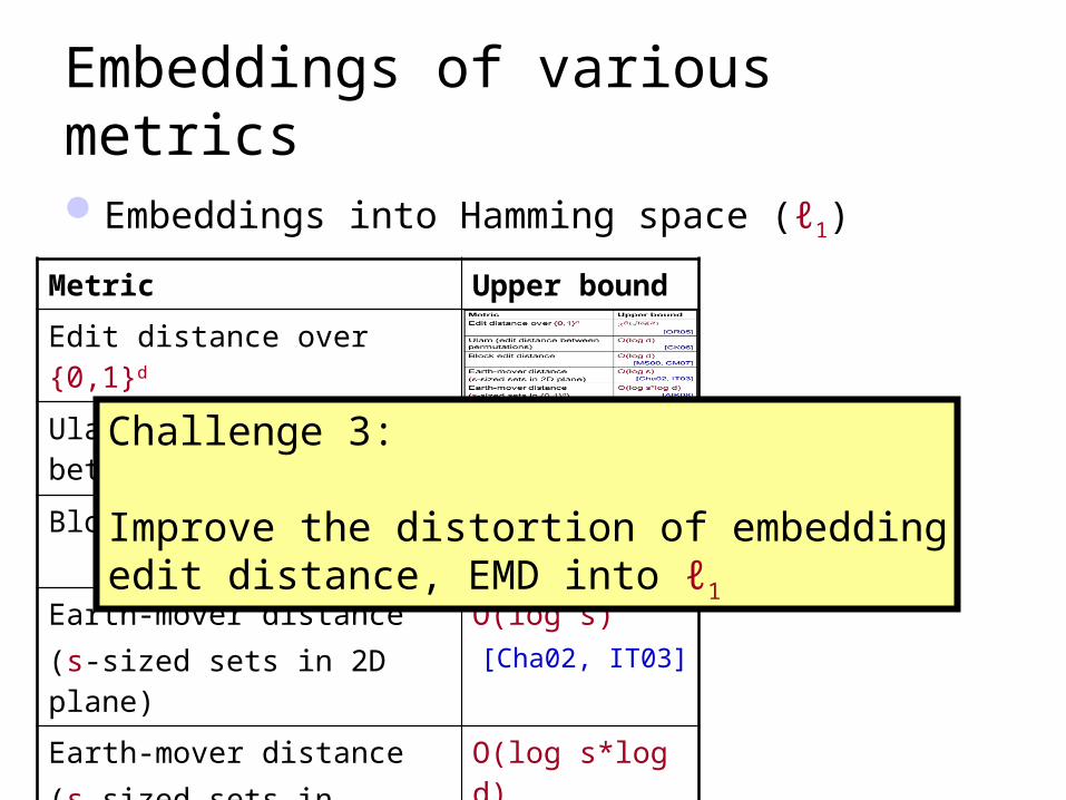
Embeddings of various metrics
Embeddings into Hamming space (ℓ1)
Metric Upper bound
Edit distance over 0,1d
Ulam (edit distance between permutations)
O(log d)[CK06]
Block edit distance O(log d)[MS00, CM07]
Earth-mover distance(s-sized sets in 2D plane)
O(log s)[Cha02, IT03]
Earth-mover distance(s-sized sets in 0,1d)
O(log s*log d)[AIK08]
Challenge 3:
Improve the distortion of embeddingedit distance, EMD into ℓ1
Are we done?“just” remains to find an embedding
with low distortion…
No, unfortunately
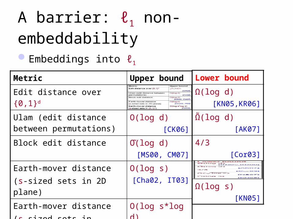
A barrier: ℓ1 non-embeddability
Embeddings into ℓ1
Metric Upper bound
Edit distance over 0,1d
Ulam (edit distance between permutations)
O(log d)[CK06]
Block edit distance O(log d)[MS00, CM07]
Earth-mover distance(s-sized sets in 2D plane)
O(log s)[Cha02, IT03]
Earth-mover distance(s-sized sets in 0,1d)
O(log s*log d)[AIK08]
Lower bound
Ω(log d)[KN05,KR06]
Ω(log d)[AK07]
4/3[Cor03]
Ω(log s)[KN05]
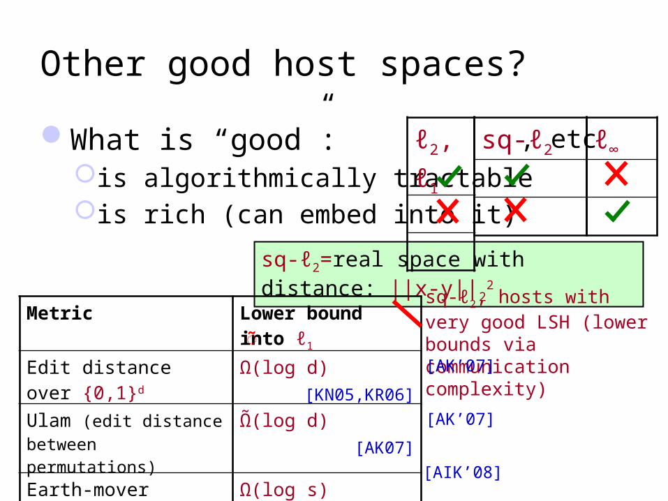
Other good host spaces?
What is “good”:is algorithmically tractableis rich (can embed into it)
sq-ℓ2=real space with distance: ||x-y||22
Metric Lower bound into ℓ1
Edit distance over 0,1d Ω(log d)[KN05,KR06]
Ulam (edit distance between permutations)
Ω(log d)[AK07]
Earth-mover distance(s-sized sets in 0,1d)
Ω(log s)[KN05]
sq-ℓ2, hosts with very good LSH (lower bounds via communication complexity)!
[AK’07]
[AK’07]
[AIK’08]
sq-ℓ2 ℓ∞, etcℓ2, ℓ1
Plan for today
1. NNS for basic distances
2. NNS for advanced distances: reductions
3. NNS via composition
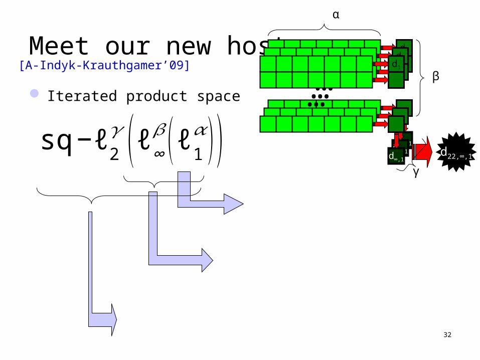
Meet our new host
Iterated product space
32
[A-Indyk-Krauthgamer’09]
d∞,1
d1
… β
α
γ
d1
…
d∞,1
d1
…
d∞,1d22,∞,1
sq −ℓ2𝛾 (ℓ∞𝛽 (ℓ1𝛼 ) )
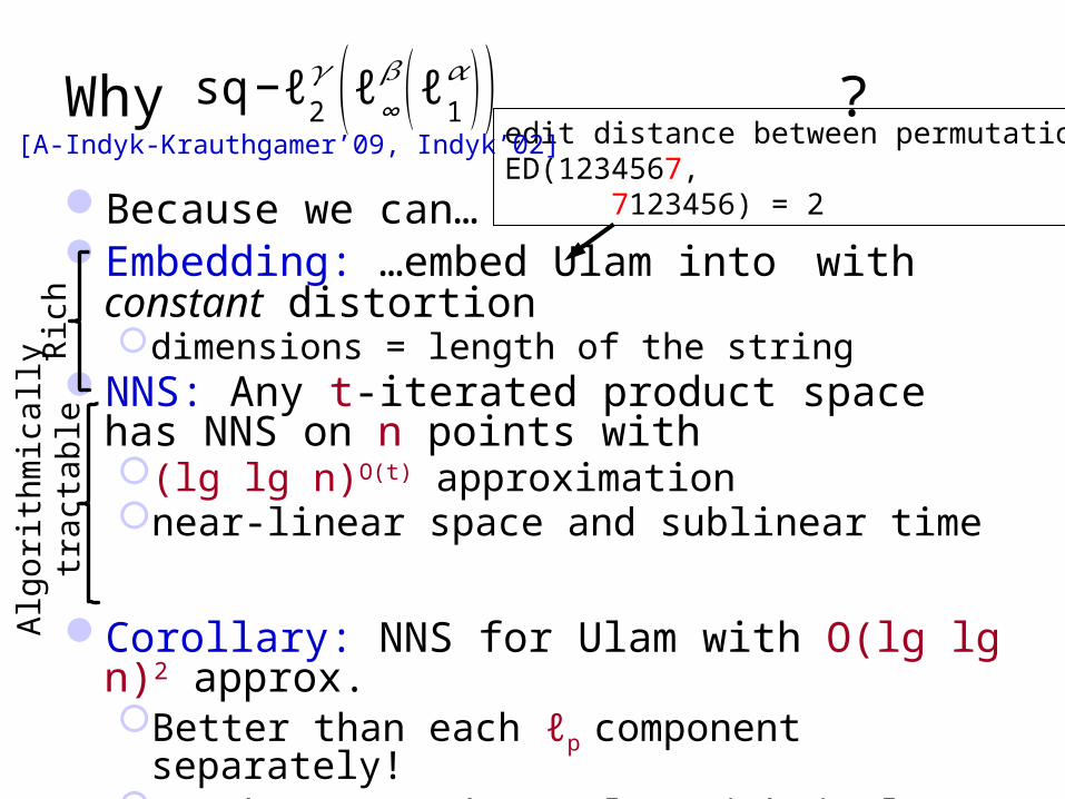
Why ?
Because we can…Embedding: …embed Ulam into with constant
distortion dimensions = length of the string
NNS: Any t-iterated product space has NNS on n points with(lg lg n)O(t) approximation near-linear space and sublinear time
Corollary: NNS for Ulam with O(lg lg n)2 approx.Better than each ℓp component separately!(each ℓp part has a logarithmic lower bound)
edit distance between permutationsED(1234567, 7123456) = 2
[A-Indyk-Krauthgamer’09, Indyk’02]
sq −ℓ2𝛾 (ℓ∞𝛽 (ℓ1𝛼 ) )
Ric
hA
lgor
ithm
ical
lytr
acta
ble
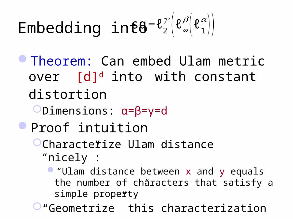
Embedding into
Theorem: Can embed Ulam metric over [d]d into with constant distortion Dimensions: α=β=γ=d
Proof intuitionCharacterize Ulam distance “nicely”:
“Ulam distance between x and y equals the number of characters that satisfy a simple property”
“Geometrize” this characterization
sq −ℓ2𝛾 (ℓ∞𝛽 (ℓ1𝛼 ) )
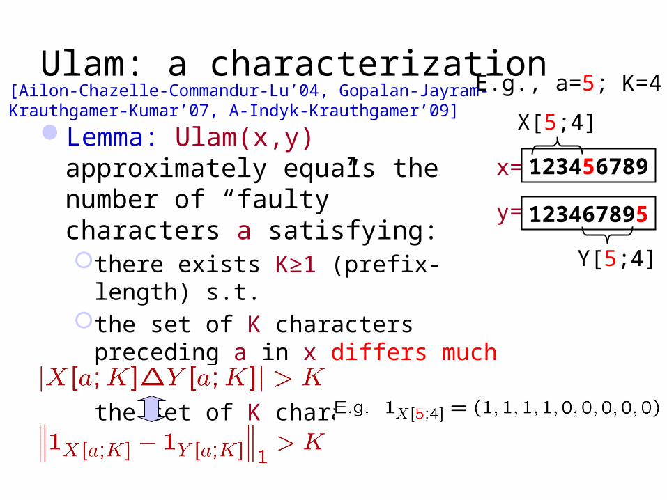
Ulam: a characterization
Lemma: Ulam(x,y) approximately equals the number of “faulty” characters a satisfying:there exists K≥1 (prefix-length) s.t.the set of K characters preceding a in x
differs much from
the set of K characters preceding a in y
123456789
123467895
Y[5;4]
X[5;4]
x=
y=
E.g., a=5; K=4[Ailon-Chazelle-Commandur-Lu’04, Gopalan-Jayram-Krauthgamer-Kumar’07, A-Indyk-Krauthgamer’09]
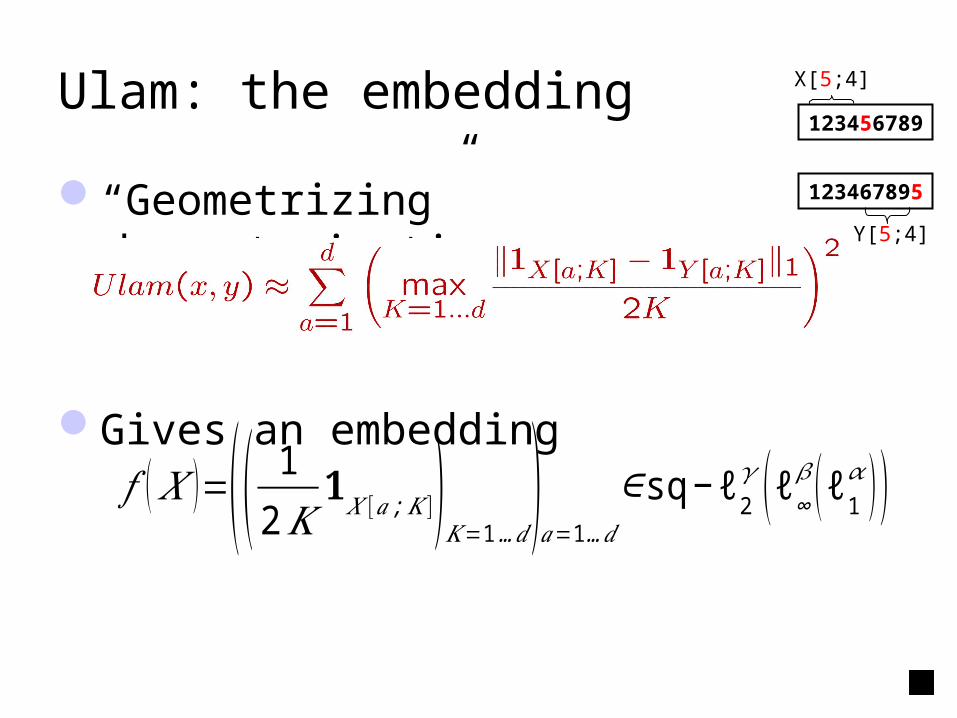
Ulam: the embedding
“Geometrizing” characterization:
Gives an embedding
123456789
123467895
Y[5;4]
X[5;4]
𝑓 ( 𝑋 )=(( 12𝐾 𝟏𝑋 [𝑎 ;𝐾 ])𝐾=1…𝑑
)𝑎=1…𝑑
∈ sq−ℓ2𝛾 (ℓ∞𝛽 (ℓ1𝛼 ))
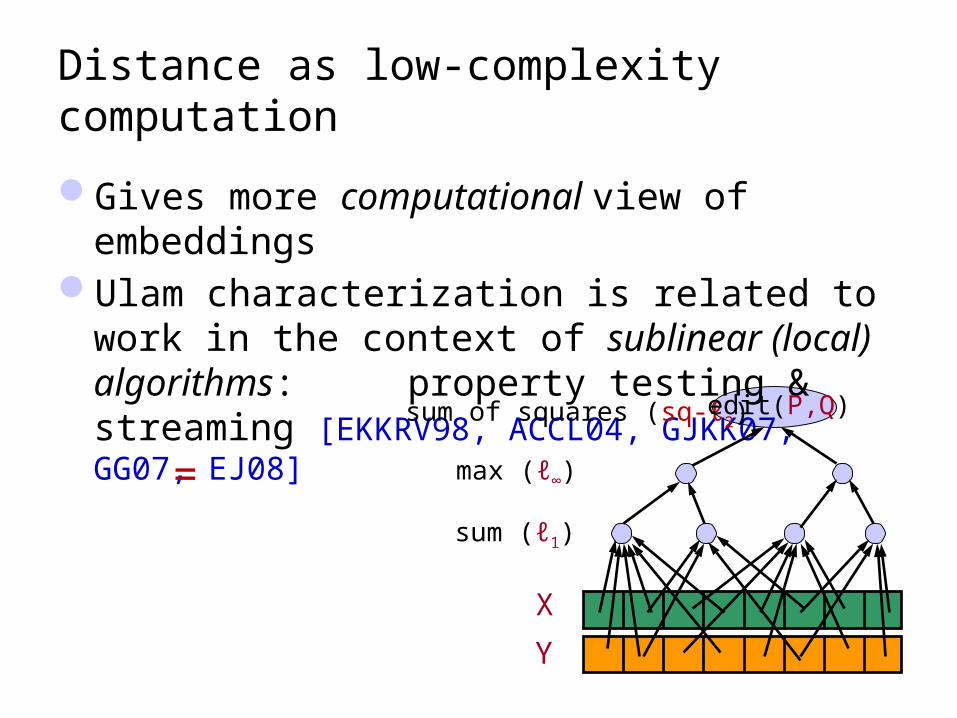
Distance as low-complexity computation
Gives more computational view of embeddingsUlam characterization is related to work in the
context of sublinear (local) algorithms: property testing & streaming [EKKRV98, ACCL04, GJKK07, GG07, EJ08]
X
Y
sum (ℓ1)
max (ℓ∞)
sum of squares (sq-ℓ2) edit(P,Q)
=
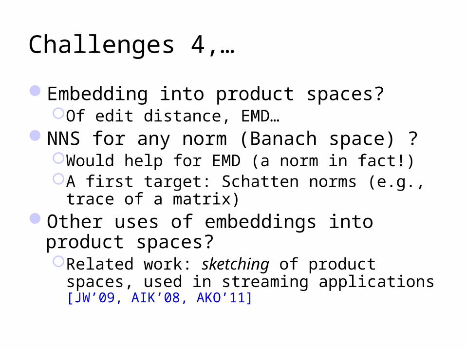
Challenges 4,…
Embedding into product spaces?Of edit distance, EMD…
NNS for any norm (Banach space) ?Would help for EMD (a norm in fact!)A first target: Schatten norms (e.g., trace of a
matrix)Other uses of embeddings into product
spaces?Related work: sketching of product spaces, used in
streaming applications [JW’09, AIK’08, AKO’11]
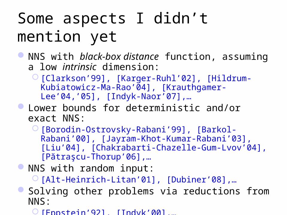
Some aspects I didn’t mention yet
NNS with black-box distance function, assuming a low intrinsic dimension: [Clarkson’99], [Karger-Ruhl’02], [Hildrum-Kubiatowicz-Ma-
Rao’04], [Krauthgamer-Lee’04,’05], [Indyk-Naor’07],…Lower bounds for deterministic and/or exact NNS:
[Borodin-Ostrovsky-Rabani’99], [Barkol-Rabani’00], [Jayram-Khot-Kumar-Rabani’03], [Liu’04], [Chakrabarti-Chazelle-Gum-Lvov’04], [Pătraşcu-Thorup’06],…
NNS with random input: [Alt-Heinrich-Litan’01], [Dubiner’08],…
Solving other problems via reductions from NNS: [Eppstein’92], [Indyk’00],…
Many others !
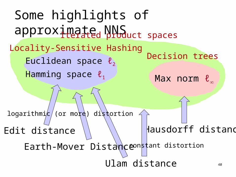
Some highlights of approximate NNS
40
Locality-Sensitive Hashing
Euclidean space ℓ2
Hamming space ℓ1
Decision trees
Max norm ℓ
Hausdorff distance
Iterated product spaces
Ulam distance
logarithmic (or more) distortion
constant distortion
Edit distance
Earth-Mover Distance
Some challenges
1. Design qualitative, efficient space partitioning in Euclidean space
2. O(1) approximation NNS for ℓ3. Embeddings with improved distortion of
edit distance, Earth-Mover Distance:into ℓ1
into product spaces
4. NNS for any norm: e.g. trace norm?
sq −ℓ2𝛾 (ℓ∞𝛽 (ℓ1𝛼 ) )