NEAR–CRITICAL PATH ANALYSIS OF PARALLEL …rbbrigh/papers/R_Brightwell94.pdf · NEAR–CRITICAL PATH ANALYSIS OF PARALLEL PROGRAM PERFORMANCE: THE STATISTICAL PERSPECTIVE By Ronald

NEAR–CRITICAL PATH ANALYSIS OF

PARALLEL PROGRAM PERFORMANCE:

THE STATISTICAL PERSPECTIVE

By

Ronald Brian Brightwell

A Thesis Submitted to the Faculty ofMississippi State University

in Partial Fulfillment of the Requirementsfor the Degree of Master of Sciencein the Department of Computer Science

Mississippi State, Mississippi

December 1994

NEAR–CRITICAL PATH ANALYSIS OF

PARALLEL PROGRAM PERFORMANCE:

THE STATISTICAL PERSPECTIVE

By

Ronald Brian Brightwell

Approved:

______________________________ _____________________________Donna S. Reese R. Rainey LittleAssistant Professor of Associate Professor ofComputer Science Computer Science(Major Professor and (Committee member)Director of Thesis)

______________________________ _____________________________Susan M. Bridges Lois C. BoggessAssistant Professor of Professor ofComputer Science Computer Science(Committee member) (Graduate Coordinator of the

Department of ComputerScience)

______________________________ _____________________________Robert A. Altenkirch Richard D. KoshelDean of the Dean of theCollege of Engineering Graduate School

Name: Ronald Brian Brightwell

Date of Degree: December 19, 1994

Institution: Mississippi State University

Major Field: Computer Science

Major Professor: Dr. Donna S. Reese

Title of Study: NEAR–CRITICAL PATH ANALYSIS OF PARALLELPROGRAM PERFORMANCE: THE STATISTICALPERSPECTIVE

Pages in Study: 76

Candidate for Degree of Master of Science

This study investigates the effectiveness of a new

parallel program performance debugging metric. The Maximum

Benefit metric is an extension of the Critical Path metric,

and is the key component in a previously proposed

near–critical path analysis framework. A prototype

implementation of this framework is presented and discussed,

along with the evaluation of the effectiveness of the

Maximum Benefit metric.

ii

ACKNOWLEDGEMENTS

First, I would like to extend sincere thanks and

appreciation to Dr. Donna Reese and Dr. Cedell Alexander for

their part in this research. I am grateful to Dr. Reese for

giving me the opportunity to work for her, and I am thankful

for her patience and guidance. I am indebted to Dr.

Alexander both for the willingness to share his research

efforts and for the direction he has given to mine.

Secondly, I would like to thank Dr. Susan Bridges and

Dr. Rainey Little for their time and efforts as members of

my graduate committee.

Finally, I would like to thank the members of the

System Software thrust at the MSU/NSF Engineering Research

Center and the members of the Computer Science department

faculty in general for all of the knowledge that they have

passed on to me.

iii

TABLE OF CONTENTS

Page

ACKNOWLEDGEMENTS ii. . . . . . . . . . . . . . . . . . . . . . . . . . . . . . . . . . . . . . . . . . . . . .

LIST OF TABLES vi. . . . . . . . . . . . . . . . . . . . . . . . . . . . . . . . . . . . . . . . . . . . . . .

LIST OF FIGURES vii. . . . . . . . . . . . . . . . . . . . . . . . . . . . . . . . . . . . . . . . . . . . . . .

CHAPTER

I. INTRODUCTION 1. . . . . . . . . . . . . . . . . . . . . . . . . . . . . . . . . . . . . . . . . .

Hypothesis 4. . . . . . . . . . . . . . . . . . . . . . . . . . . . . . . . . . . . . . . . . . . . Objectives 5. . . . . . . . . . . . . . . . . . . . . . . . . . . . . . . . . . . . . . . . . . . . Overview 5. . . . . . . . . . . . . . . . . . . . . . . . . . . . . . . . . . . . . . . . . . . . . .

II. REVIEW OF LITERATURE 7. . . . . . . . . . . . . . . . . . . . . . . . . . . . . . . . IPS 7. . . . . . . . . . . . . . . . . . . . . . . . . . . . . . . . . . . . . . . . . . . . . . . . . . . .

Critical Path Analysis 8. . . . . . . . . . . . . . . . . . . . . . . . . . . IPS–2 Profiling 9. . . . . . . . . . . . . . . . . . . . . . . . . . . . . . . . . . . Slack 9. . . . . . . . . . . . . . . . . . . . . . . . . . . . . . . . . . . . . . . . . . . . . . . Logical Zeroing 10. . . . . . . . . . . . . . . . . . . . . . . . . . . . . . . . . . . Phase Behavior Analysis 10. . . . . . . . . . . . . . . . . . . . . . . . .

PargGraph 11. . . . . . . . . . . . . . . . . . . . . . . . . . . . . . . . . . . . . . . . . . . . . Critical Path Display 12. . . . . . . . . . . . . . . . . . . . . . . . . . . . Phase Portrait Display 12. . . . . . . . . . . . . . . . . . . . . . . . . . .

Quartz 13. . . . . . . . . . . . . . . . . . . . . . . . . . . . . . . . . . . . . . . . . . . . . . . . . Normalized Processor Time 14. . . . . . . . . . . . . . . . . . . . . . .

The Performance Consultant 15. . . . . . . . . . . . . . . . . . . . . . . . . “Why” Axis 16. . . . . . . . . . . . . . . . . . . . . . . . . . . . . . . . . . . . . . . . . “Where” Axis 16. . . . . . . . . . . . . . . . . . . . . . . . . . . . . . . . . . . . . . . “When” Axis 17. . . . . . . . . . . . . . . . . . . . . . . . . . . . . . . . . . . . . . . . Hints 17. . . . . . . . . . . . . . . . . . . . . . . . . . . . . . . . . . . . . . . . . . . . . . .

Projections 18. . . . . . . . . . . . . . . . . . . . . . . . . . . . . . . . . . . . . . . . . . . The Analysis Component 19. . . . . . . . . . . . . . . . . . . . . . . . . . . Information Sharing Branch 19. . . . . . . . . . . . . . . . . . . . . .

iv

CHAPTER Page

Critical Path Analysis Branch 20. . . . . . . . . . . . . . . . . . ATExpert 21. . . . . . . . . . . . . . . . . . . . . . . . . . . . . . . . . . . . . . . . . . . . . .

Parallel Region Monitor 21. . . . . . . . . . . . . . . . . . . . . . . . . Subroutine Window 22. . . . . . . . . . . . . . . . . . . . . . . . . . . . . . . . . Parallel Region Window 22. . . . . . . . . . . . . . . . . . . . . . . . . . . Loop Window 23. . . . . . . . . . . . . . . . . . . . . . . . . . . . . . . . . . . . . . . .

Evaluation of Guidance Techniques 24. . . . . . . . . . . . . . . . The Maximum Benefit Metric 28. . . . . . . . . . . . . . . . . . . . . . . . . Near–Critical Path Performance

Analysis Framework 29. . . . . . . . . . . . . . . . . . . . . . . . . . . . . . . Choice of the Pablo Performance

Analysis Environment 29. . . . . . . . . . . . . . . . . . . . . . . . . . . . .

III. APPROACH 32. . . . . . . . . . . . . . . . . . . . . . . . . . . . . . . . . . . . . . . . . . . . . . Methodology 32. . . . . . . . . . . . . . . . . . . . . . . . . . . . . . . . . . . . . . . . . . .

MSPARC Multicomputer InstrumentationSystem 32. . . . . . . . . . . . . . . . . . . . . . . . . . . . . . . . . . . . . . . . . . .

Object–Oriented Fortran 33. . . . . . . . . . . . . . . . . . . . . . . . . Object Information File 34. . . . . . . . . . . . . . . . . . . . . . . . . Program Activity Graphs 34. . . . . . . . . . . . . . . . . . . . . . . . .

Application Programs 36. . . . . . . . . . . . . . . . . . . . . . . . . . . . . . . . Lower–Upper Solver 36. . . . . . . . . . . . . . . . . . . . . . . . . . . . . . . Asynchronous Near–Critical Path

Analyzer 37. . . . . . . . . . . . . . . . . . . . . . . . . . . . . . . . . . . . . . . . Maximum Benefit Metric Calculation 38. . . . . . . . . . . . . . .

Calculation 38. . . . . . . . . . . . . . . . . . . . . . . . . . . . . . . . . . . . . . . . Presentation 40. . . . . . . . . . . . . . . . . . . . . . . . . . . . . . . . . . . . . . .

What If Scenario 40. . . . . . . . . . . . . . . . . . . . . . . . . . . . . . . . . . . . . Pablo Module Development 41. . . . . . . . . . . . . . . . . . . . . . . . . . .

Labeled Multi–Bargraph 42. . . . . . . . . . . . . . . . . . . . . . . . . . . String Printer 43. . . . . . . . . . . . . . . . . . . . . . . . . . . . . . . . . . . .

Metric Comparison 43. . . . . . . . . . . . . . . . . . . . . . . . . . . . . . . . . . . .

IV. RESULTS 45. . . . . . . . . . . . . . . . . . . . . . . . . . . . . . . . . . . . . . . . . . . . . . . . Maximum Benefit Metric 45. . . . . . . . . . . . . . . . . . . . . . . . . . . . . .

LU Results 45. . . . . . . . . . . . . . . . . . . . . . . . . . . . . . . . . . . . . . . . . CNCP Results 47. . . . . . . . . . . . . . . . . . . . . . . . . . . . . . . . . . . . . . . JUL Results 47. . . . . . . . . . . . . . . . . . . . . . . . . . . . . . . . . . . . . . . . EP Results 48. . . . . . . . . . . . . . . . . . . . . . . . . . . . . . . . . . . . . . . . . SP Results 48. . . . . . . . . . . . . . . . . . . . . . . . . . . . . . . . . . . . . . . . . QSORT Results 51. . . . . . . . . . . . . . . . . . . . . . . . . . . . . . . . . . . . .

v

CHAPTER Page

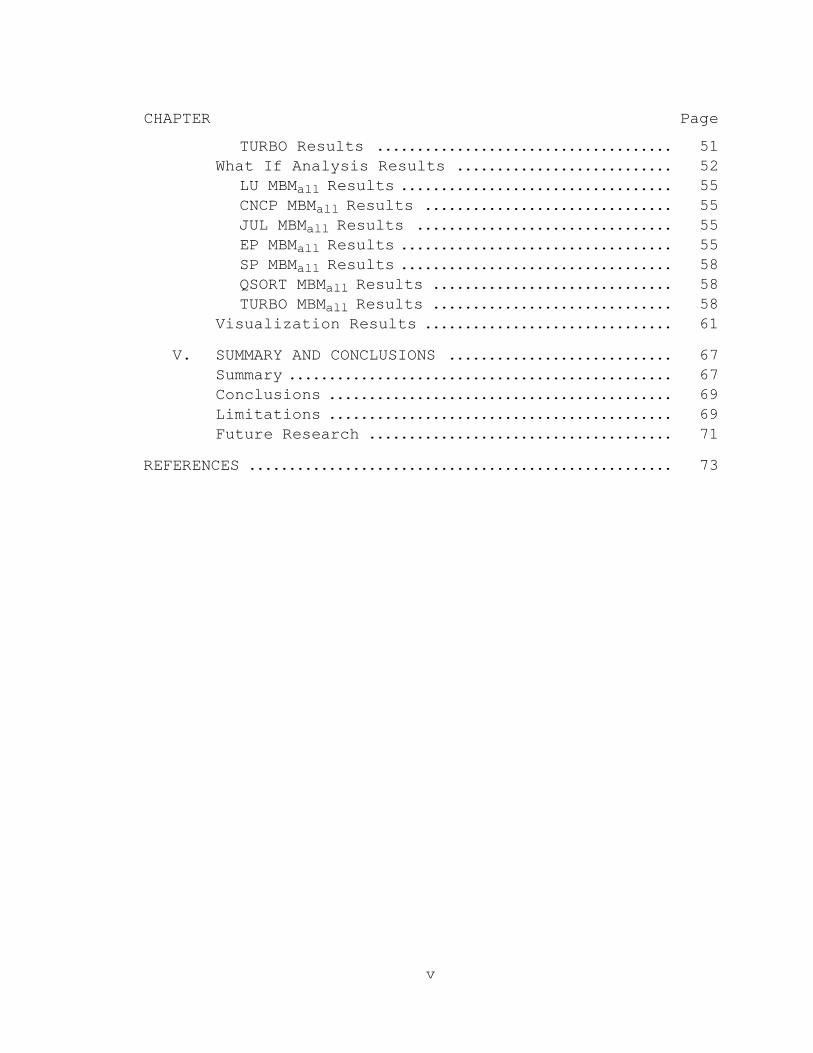
TURBO Results 51. . . . . . . . . . . . . . . . . . . . . . . . . . . . . . . . . . . . . What If Analysis Results 52. . . . . . . . . . . . . . . . . . . . . . . . . . .

LU MBMall Results 55. . . . . . . . . . . . . . . . . . . . . . . . . . . . . . . . . . CNCP MBMall Results 55. . . . . . . . . . . . . . . . . . . . . . . . . . . . . . . JUL MBMall Results 55. . . . . . . . . . . . . . . . . . . . . . . . . . . . . . . . EP MBMall Results 55. . . . . . . . . . . . . . . . . . . . . . . . . . . . . . . . . . SP MBMall Results 58. . . . . . . . . . . . . . . . . . . . . . . . . . . . . . . . . . QSORT MBMall Results 58. . . . . . . . . . . . . . . . . . . . . . . . . . . . . . TURBO MBMall Results 58. . . . . . . . . . . . . . . . . . . . . . . . . . . . . .

Visualization Results 61. . . . . . . . . . . . . . . . . . . . . . . . . . . . . . .

V. SUMMARY AND CONCLUSIONS 67. . . . . . . . . . . . . . . . . . . . . . . . . . . . Summary 67. . . . . . . . . . . . . . . . . . . . . . . . . . . . . . . . . . . . . . . . . . . . . . . . Conclusions 69. . . . . . . . . . . . . . . . . . . . . . . . . . . . . . . . . . . . . . . . . . . Limitations 69. . . . . . . . . . . . . . . . . . . . . . . . . . . . . . . . . . . . . . . . . . . Future Research 71. . . . . . . . . . . . . . . . . . . . . . . . . . . . . . . . . . . . . .

REFERENCES 73. . . . . . . . . . . . . . . . . . . . . . . . . . . . . . . . . . . . . . . . . . . . . . . . . . . . .

vi

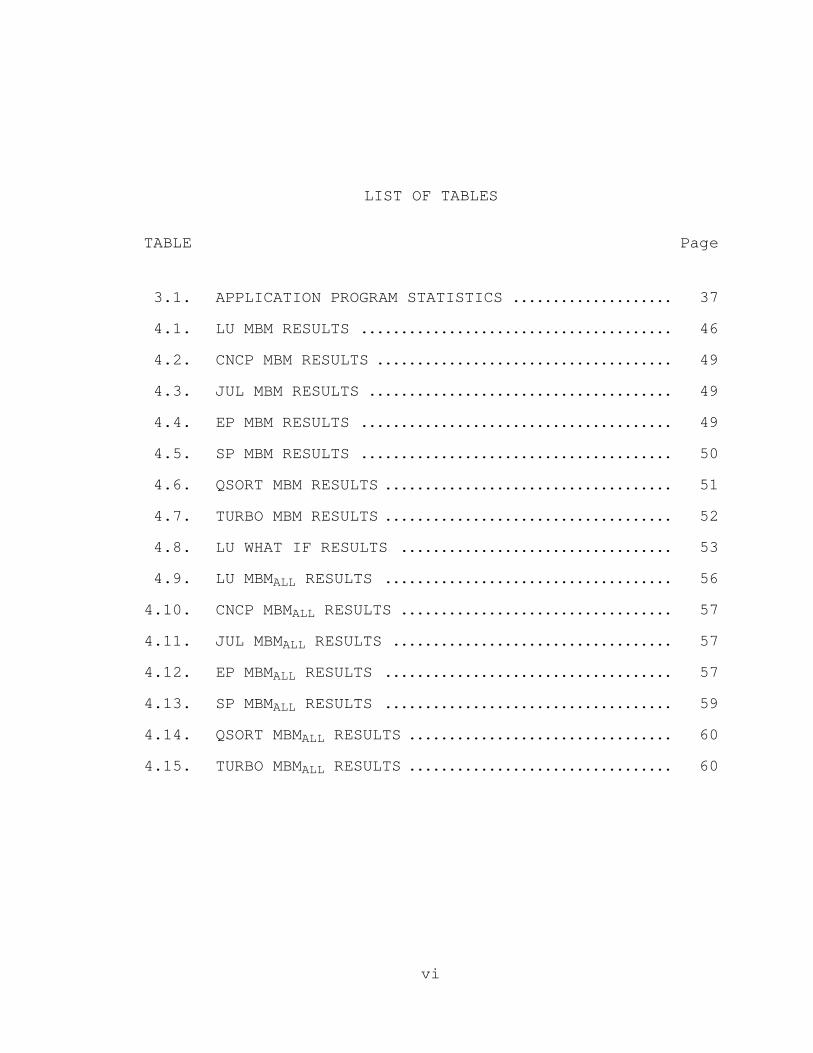
LIST OF TABLES

TABLE Page

3.1. APPLICATION PROGRAM STATISTICS 37. . . . . . . . . . . . . . . . . . . .

4.1. LU MBM RESULTS 46. . . . . . . . . . . . . . . . . . . . . . . . . . . . . . . . . . . . . . .

4.2. CNCP MBM RESULTS 49. . . . . . . . . . . . . . . . . . . . . . . . . . . . . . . . . . . . .

4.3. JUL MBM RESULTS 49. . . . . . . . . . . . . . . . . . . . . . . . . . . . . . . . . . . . . .

4.4. EP MBM RESULTS 49. . . . . . . . . . . . . . . . . . . . . . . . . . . . . . . . . . . . . . .

4.5. SP MBM RESULTS 50. . . . . . . . . . . . . . . . . . . . . . . . . . . . . . . . . . . . . . .

4.6. QSORT MBM RESULTS 51. . . . . . . . . . . . . . . . . . . . . . . . . . . . . . . . . . . .

4.7. TURBO MBM RESULTS 52. . . . . . . . . . . . . . . . . . . . . . . . . . . . . . . . . . . .

4.8. LU WHAT IF RESULTS 53. . . . . . . . . . . . . . . . . . . . . . . . . . . . . . . . . .

4.9. LU MBMALL RESULTS 56. . . . . . . . . . . . . . . . . . . . . . . . . . . . . . . . . . . .

4.10. CNCP MBMALL RESULTS 57. . . . . . . . . . . . . . . . . . . . . . . . . . . . . . . . . .

4.11. JUL MBMALL RESULTS 57. . . . . . . . . . . . . . . . . . . . . . . . . . . . . . . . . . .

4.12. EP MBMALL RESULTS 57. . . . . . . . . . . . . . . . . . . . . . . . . . . . . . . . . . . .

4.13. SP MBMALL RESULTS 59. . . . . . . . . . . . . . . . . . . . . . . . . . . . . . . . . . . .

4.14. QSORT MBMALL RESULTS 60. . . . . . . . . . . . . . . . . . . . . . . . . . . . . . . . .

4.15. TURBO MBMALL RESULTS 60. . . . . . . . . . . . . . . . . . . . . . . . . . . . . . . . .

vii

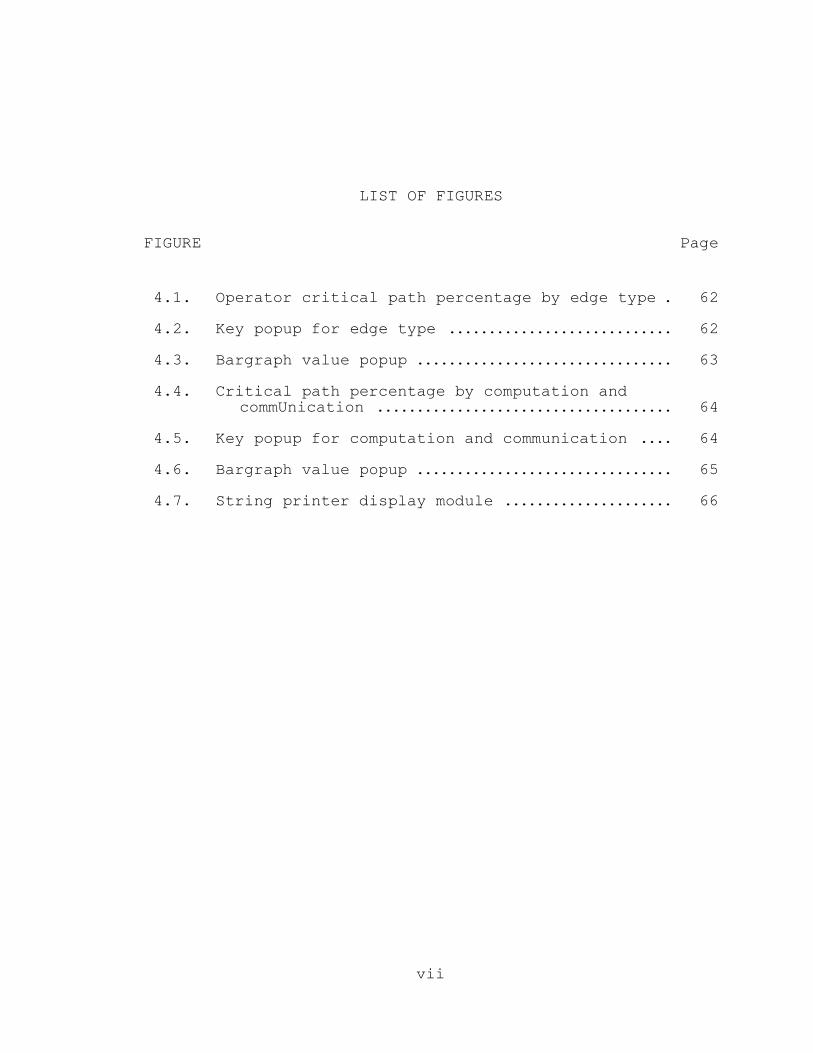
LIST OF FIGURES

FIGURE Page

4.1. Operator critical path percentage by edge type 62.

4.2. Key popup for edge type 62. . . . . . . . . . . . . . . . . . . . . . . . . . . .

4.3. Bargraph value popup 63. . . . . . . . . . . . . . . . . . . . . . . . . . . . . . . .

4.4. Critical path percentage by computation andcommUnication 64. . . . . . . . . . . . . . . . . . . . . . . . . . . . . . . . . . . . .

4.5. Key popup for computation and communication 64. . . .

4.6. Bargraph value popup 65. . . . . . . . . . . . . . . . . . . . . . . . . . . . . . . .

4.7. String printer display module 66. . . . . . . . . . . . . . . . . . . . .

1

CHAPTER I

INTRODUCTION

Monitoring the performance of parallel application

programs has been the subject of extensive research over the

past decade. The need to observe the characteristics of

parallel programs for the purposes of debugging and refining

applications has been apparent since the feasibility of

utilizing multiple processors to maximize the performance of

computing applications. The main goal of performance

monitoring is to provide the application programmer with the

information needed to construct and modify programs and

algorithms in order to make effective use of available

computing power. There are several factors involved in

parallel programming that reinforce the need for detailed

examination, such as nondeterministic and sometimes

unpredictable behavior. In most cases, a problem is

parallelized to decrease the amount of time needed to

achieve the desired solution. To better understand the

activities of a parallel system, insight into execution

behavior is necessary, especially where the exhibited

behavior is inefficient or incorrect.

2

Early research in the field of performance monitoring

focused on the extraction of meaningful information from the

execution of a parallel application program. Much research

was devoted to identifying the key events that represented

program execution and developing systems that gathered this

information. Further research was directed at the most

efficient manner in which to collect and analyze event

information. Performance monitoring systems were designed to

gather the greatest amount of information with the least

amount of interference or perturbation. More recently, the

focus has moved from the interaction of the parallel program

and the monitoring system to the interaction of the

monitoring system and the user. In much the same way the

feasibility of parallel processing led to the need to take

advantage of increased computing power, the feasibility of

effective performance monitoring systems has led to the need

to take advantage of the increase in valuable information

that these systems offer. Providing the programmer with the

type of information needed to improve the performance of the

parallel program has become paramount.

The abundance of data that can be obtained from

performance monitoring systems has the potential to be

overwhelming. Currently, much research is being devoted to

conveying performance data in ways that provide the greatest

amount of understanding, both visually and aurally. The

effectiveness of any monitoring system depends on the

3

ability to correctly interpret the information that has been

collected and presented. In some systems, this

interpretation is left to the user, while other systems,

known as performance debuggers, provide facilities for

system–aided guidance in locating performance bottlenecks.

A performance debugger can utilize one of several

methods used to direct the programmer to sources of poor

program performance. Inherent in all performance monitoring

systems is the ability to calculate performance metrics to

measure or quantify certain execution characteristics.

Performance data can then be interpreted in many different

ways, through such means as metric comparison, logic–based

analysis, and rules–based analysis. The main goal of this

interpretation is to make areas of poor performance known to

the user in a way that best facilitates the discovery and

elimination of the source of the problem. A secondary goal

in many performance debugging systems is to offer advice or

make suggestions to the user concerning the manner in which

the problem may be eliminated.

One example of system–aided guidance in performance

debugging is provided through profiling metrics, which are

performance measurements that can be directly attributed to

a program’s components, such as individual procedures and

functions. Profiling metrics try to identify those program

components which are sources of poor performance in order to

focus a programmer’s optimization efforts. The ability to

4

combine the discovery of poor performance with the

responsible program components into one measurement makes

profiling metrics very attractive. Also, since results are

based on the source code, attractiveness is increased by an

innate property of scalability to massively parallel

systems.

Many profiling metrics have been developed and either

compared with existing metrics or tested on specific cases

to assess overall effectiveness. However, because of the

possibility of programmer influence in case studies, direct

comparison has proved to be the best way to evaluate a new

metric’s effectiveness (Hollingsworth and Miller 1992).

One such new profiling metric which has yet to be

tested, the Maximum Benefit metric, defined by Alexander

(1994), is a derivative of the Critical Path metric (Yang

and Miller 1989) which provides the basis for a proposed

near–critical path analysis framework that includes

performance analysis and visualization capabilities.

Hypothesis

It is the hypothesis of this research that the Maximum

Benefit metric will reveal additional characteristics about

parallel program performance beyond that of the traditional

Critical Path metric, and that, along with other components

of the near–critical path analysis framework, it can provide

the basis for additional performance monitoring tools.

5

Objectives

There are several goals related to this research,

foremost of which is to determine the effectiveness of the

Maximum Benefit metric in relation to the Critical Path

metric. Secondly, this research should build a foundation

for an additional set of performance monitoring tools based

upon the near–critical path concept, and relate the

knowledge obtained from the use of the components of the

analysis framework. And the final objective of this study

is to provide direction to future researchers who plan to

build upon the results of this research.

Overview

In the next chapter, several performance monitoring

systems will be examined, along with tools that attempt to

provide guidance to the user in finding and correcting areas

of poor performance. The advantages and disadvantages of

these tools will be discussed, the Maximum Benefit metric

will be formally defined, and the previously proposed

analysis framework will be described.

The third chapter presents an approach to the

implementation of the proposed analysis framework and a

description of the methods used for testing the hypothesis.

The results of the collected data will be discussed in the

fourth chapter, and the final chapter will present a summary

of the research in relation to the initial hypothesis,

6

identify any unexpected results, and provide some direction

and ideas for future research.

7

CHAPTER II

REVIEW OF LITERATURE

This chapter introduces several performance monitoring

systems and focuses on some of the metrics and analysis

techniques that are intended to provide guidance to the

programmer for finding performance bottlenecks. The

advantages and disadvantages of these methods will be

discussed, followed by a description of the proposed

near–critical path analysis framework and the definition of

the Maximum Benefit metric.

IPS

IPS (Yang and Miller 1989) and the second

implementation IPS–2 (Miller et al. 1990), developed at the

University of Wisconsin, are performance monitoring systems

for parallel and distributed programs. IPS is based on a

hierarchical model that presents multiple levels of

abstraction along with multiple views of performance data.

IPS was designed to bridge the gap between the structure of

parallel programs and the structure of performance

monitoring systems, and also the gap between what users need

to know and what systems provide. One of the main goals of

IPS was to provide programmers some direction in locating

8

performance problems, and a system that would “provide

answers, not just numbers” (Yang and Miller 1989). Past

experience with performance monitoring systems had shown

that traditional metrics revealed the existence of poor

performance, but failed to reveal the cause of poor

performance. IPS attempts to steer the programmer toward

performance bottlenecks through automatic guidance

techniques consisting of performance metrics and data

analysis. The automatic guidance features of IPS are

Critical Path Analysis, IPS–2 Profiling, Slack, Logical

Zeroing, and Phase Behavior Analysis.

Critical Path Analysis

Critical Path Analysis (CPA) (Miller et al. 1990)

involves constructing a Program Activity Graph (PAG) from

data collected during program execution. The PAG is a

weighted, directed, acyclic multigraph that represents the

precedence relationship among program activities. Edges in

the graph represent specific program activities while the

weight of an edge represents the duration of the

corresponding activity. Vertices represent the start and

finish of activities, marking activity boundaries. The

critical path in a PAG is the path with the longest total

duration and is the path that is responsible for the overall

execution time of the application program. CPA discovers

the critical path and identifies the specific events

9

(procedures and functions) or sequences of events in the

program that lie on the critical path. All of the

procedures and functions of the user program are ranked

according to the percentage of the critical path for which

each is responsible. As with all IPS data, critical path

statistics can be viewed on the program, machine, process,

and procedure levels of abstraction. The data is presented

to the user in tabular form.

IPS–2 Profiling

IPS–2 Profiling (Miller et al. 1990) is an extension of

the standard UNIX Gprof profiling tool (Graham, Kessler, and

McKusick 1982). Gprof is a call graph profiler which

computes the total time spent in each procedure for each

process or sequential application program. Most

implementations of Gprof use periodic sampling of the

program counter to calculate this metric for all procedures.

The effectiveness of the Gprof metric in a multi–processor

environment is limited by the inability to distinguish

between useful computation and busy waiting time. IPS–2

Profiling uses a PAG to make this distinction and, by

ignoring all inter–process arcs, computes only the total

useful CPU time spent in each procedure.

Slack

Slack (Miller et al. 1990) is a metric which attempts

to quantify the benefit which may be obtained by reducing

10

the execution time of a procedure on the critical path. All

of the procedures on the critical path are assigned a slack

value as an optimization threshold. If the execution time

of a procedure is reduced beyond this value, the critical

path will be altered. Slack was motivated by the need to

analyze the relationship between the critical path and the

secondary paths in a PAG.

Logical Zeroing

Logical Zeroing (Miller et al. 1990) examines a PAG for

a particular application and attempts to estimate the

improvement that could be gained from optimizing a specific

procedure or function. The metric is calculated by zeroing

the duration of a particular activity in the PAG and then

recalculating the length of the Critical Path. The

difference in the duration of the Critical Path of the

original graph and the duration of the Critical Path of the

modified graph is computed. Logical Zeroing estimates the

amount of improvement that could be gained by optimizing or

improving a specific procedure which lies on the Critical

Path.

Phase Behavior Analysis

Phase Behavior Analysis (PBA) (Miller et al. 1990)

attempts to identify the different phases that a parallel

program may go through during execution. A phase of a

program is defined as a period of time when consistent

11

values are maintained by a set of performance metrics. IPS

implements a phase detection algorithm which analyzes metric

data in an attempt to find those areas of a program where

behavior is somewhat uniform. PBA data is presented to the

user as a graph where the appropriate metrics are plotted

over time and the phases are identified by boundary lines

perpendicular to the time axis. PBA is intended to focus

the attention of the user on specific segments in the

program so periods of poor performance can be more easily

identified and so that each phase may be treated as a

separate problem.

ParaGraph

ParaGraph (Heath and Etheridge 1991), developed at Oak

Ridge National Laboratory, is a performance monitoring

system for visualizing the behavior of parallel programs on

message–passing multiprocessor architectures. The key

emphasis in ParaGraph is on the visualization that is used

to gain insight into the behavior of the program. ParaGraph

provides graphical animation of the message–passing

activities as well as graphical summaries of program

performance. ParaGraph distinguished itself from previous

performance visualization tools by providing a greater

variety of perspectives and views, and by emphasizing

portability, extensibility, and ease of use. ParaGraph uses

the trace data provided by the Portable Instrumented

12

Communication Library (PICL) (Geist et al. 1992) for

building its utilization, communication, and task

information displays. Along with the many different types

of standard displays, ParaGraph also has Critical Path and

Phase Portrait displays.

Critical Path Display

In the Critical Path display (Heath and Etheridge

1991), processor number is displayed on the vertical axis,

while time is on the horizontal axis, which moves as time

proceeds. The activity on a processor is shown by a

horizontal line for each processor which increases in width

as the processor becomes busy, while communication between

processors is shown by slanted lines between the

communicating processors. Processor and message lines that

are on the Critical Path are highlighted to show the longest

serial thread in the parallel computation. The display is

meant to guide the user to specific areas of the program

where performance is being limited. The Critical Path

display only shows the processors that are involved in the

Critical Path and does not point out specific functions or

procedures which are on the Critical Path as does IPS.

Phase Portrait Display

The Phase Portrait display (Heath and Etheridge 1991)

in ParaGraph attempts to portray the relationship between

communication and processor utilization over time. The

13

percentage of busy processors is plotted against the

percentage of the maximum volume of communication currently

in transit. The resulting plot moves along the horizontal

axis as time progresses. Communication and processor

utilization are assumed to have an inverse relationship, and

therefore the plot is most likely to lie on the diagonal of

the display. Different program tasks may be color coded to

identify phases and repetitive periodic behavior. Contrary

to IPS, there is no automatic identification of different

phases.

Quartz

Quartz (Anderson and Lazowska 1990), developed at the

University of Washington, is a tool for tuning parallel

programs which utilize shared memory multiprocessors. The

inspiration for Quartz came from the UNIX Gprof profiling

tool, and the system’s main goal is to direct the attention

of the programmer first by efficiently measuring the factors

that are most responsible for performance and then by

relating these measurements to each other and to the

structure of the program. The designers of the system

wanted Quartz to measure parallelism, relate the measurement

directly to the source code, and identify where code

restructuring or optimization is needed. The chief metric

used to identify areas of poor performance is Normalized

Processor Time (NPT).

14

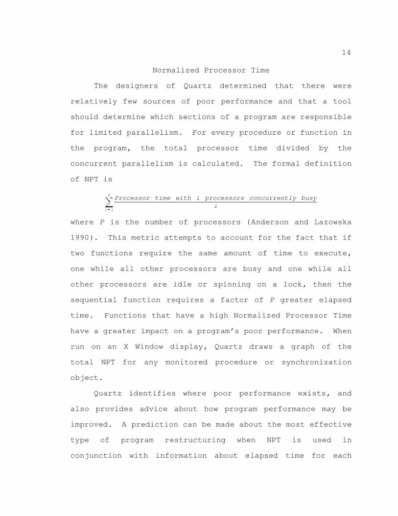
Normalized Processor Time

The designers of Quartz determined that there were

relatively few sources of poor performance and that a tool

should determine which sections of a program are responsible

for limited parallelism. For every procedure or function in

the program, the total processor time divided by the

concurrent parallelism is calculated. The formal definition

of NPT is

� P

i � 1

Processor time with i processors concurrently busyi

where P is the number of processors (Anderson and Lazowska

1990). This metric attempts to account for the fact that if

two functions require the same amount of time to execute,

one while all other processors are busy and one while all

other processors are idle or spinning on a lock, then the

sequential function requires a factor of P greater elapsed

time. Functions that have a high Normalized Processor Time

have a greater impact on a program’s poor performance. When

run on an X Window display, Quartz draws a graph of the

total NPT for any monitored procedure or synchronization

object.

Quartz identifies where poor performance exists, and

also provides advice about how program performance may be

improved. A prediction can be made about the most effective

type of program restructuring when NPT is used in

conjunction with information about elapsed time for each

15

procedure along with the average and distribution of the

number of threads available to run while the procedure is in

a ready, busy, blocked, or spinning state. For example, if

there are several threads waiting at a barrier and there are

at least as many runnable threads as there are processors,

then blocked threads have no impact upon performance.

However, if there are more runnable threads than processors,

then an improvement in performance may be gained by blocking

threads instead of spin–waiting. Quartz attempts to make

suggestions about increasing program performance through

functional decomposition, data decomposition,

synchronization, and input/output based on a combination of

NPT with other system metrics.

The Performance Consultant

The Performance Consultant is a prototype

implementation of the W3 Search Model (Hollingsworth and

Miller 1993), which is a strategy designed to answer the

three most important questions in performance monitoring:

Why, Where, and When. The main goal of the W3 Search Model

is to reduce the overload of performance data presented to

the user on massively parallel machines by providing a

logical search model that implements automatic guidance

techniques to quickly locate performance bottlenecks. The

model is described as a three dimensional space with each

question residing on an axis, and the search process

16

involves moving from point to point in this space. Movement

is facilitated by testing built–in hypotheses along each

axis.

“Why” Axis

On this axis, an iterative evaluation of hypotheses is

made in attempt to locate performance bottlenecks

(Hollingsworth and Miller 1993). Hypotheses are selected

and tested. When a hypothesis proves to be true, possible

refinements are considered. For example, if the original

hypothesis is that an application contains a performance

bottleneck, then further refinements would attempt to

pinpoint the cause of the bottleneck: improper division of

labor, high contention for a shared resource, or too much

time spent waiting for messages. Each of these refinements

would be tested in an effort to further pinpoint the source

of the poor performance. Examining the “why” axis involves

traversing the directed acyclic graph that is created by the

hierarchical relationships of the hypotheses.

“Where” Axis

The “Where” axis is very similar to the “Why” axis and

is examined in much the same way (Hollingsworth and Miller

1993). The hierarchical organization is separated into

different classes of resources, some of which are created at

start time and others of which are created dynamically as

the program executes. For example, the category of spin

17

locks could be chosen from the synchronization objects

resource class, a specific processor could be chosen from

the compute object resource class, and a specific function

could be chosen from the code resource class. Then, tests

could be run to determine the truth value of the hypothesis

for spin locks in the selected procedure on the selected

processor. The current status of this axis is known as the

focus, and each true hypothesis results in addition to a

list of current focuses. The list of focuses is reduced by

discarding a focus if the criteria for the hypothesis are

not met.

“When” Axis

This axis is used to determine the time interval during

which a performance bottleneck exists. The “when” axis is

examined by testing the current focus or focuses for

different time segments during the execution of the program

(Hollingsworth and Miller 1993). At the start, the entire

program execution time is considered, and the search is

refined by breaking the time intervals into smaller pieces.

This axis also has a hierarchical structure, with the total

execution time as the root and subsequent intervals and

sub–intervals as children nodes.

Hints

Automatic guidance is provided in W3 by hints

(Hollingsworth and Miller 1993). Hints are suggestions made

18

about possible refinements which result from the testing of

previous refinements. For example, testing a hypothesis

along one axis may lead to a hint about a refinement along a

different axis based on the outcome of a prior hypothesis.

If the Performance consultant is in the manual mode, the

user is free to ignore the hints that are offered and

proceed according to the user’s own judgements. In the

automatic mode, refinements are chosen by gathering hints,

ordering refinements based on the hints, and then selecting

the most promising refinement to pursue.

Projections

Projections (Sinha and Kalé 1994) is the display and

analysis component of a framework which provides intelligent

feedback about the performance of programs written in the

Charm (Kalé 1990) parallel programming language. This

framework is centered upon the idea that a good performance

analysis tool should not only display specific program

information, but also intelligently analyze the data in

order to find poor performance. Projections attempts to

improve upon the generality of tools such a ParaGraph (Heath

and Etheridge 1991) and Upshot (Herrarte and Lusk 1991) by

providing information specifically geared toward the

language constructs of Charm. Projections also attempts to

overcome the inability of general performance tools to scale

to hundreds of processors by allowing the performance data

19

to viewed from multiple perspectives. The entire program

execution may be analyzed through summary views, while

specific areas may be examined through detailed views (Sinha

and Kalé 1993).

The Analysis Component

The analysis component of Projections (Sinha and Kalé

1994) is based upon a decision tree where different nodes

correspond to specific program characteristics. A decision

node which identifies a time when poor performance exists is

at the root of the tree. The next level of the tree

determines whether an imbalance in processor utilization is

present and whether sufficient work exists for processors

which are performing poorly. Subsequent levels in the tree

attempt to correlate poor performance with specific program

attributes, such as grain size and message loads. The

analysis process is intended to be iterative. Feedback

results from a pass through the decision tree and

appropriate modifications are made before the analysis

component is reenvoked. Two branches of the decision tree

which try to uncover the program characteristics that are

responsible for poor performance are the information sharing

branch and the critical path analysis branch.

Information Sharing Branch

The information sharing branch examines the shared

variable accesses of a particular application (Sinha and

20

Kalé 1994). Charm contains five types of shared memory

variables: read only, write once, accumulator, monotonic,

and distributed tables. The way in which these different

types of shared variables are accessed and manipulated may

provide insight into the cause of poor performance. For

example, a distributed table is a structure which can be

queried to obtain some global information. The querying

process involves a message send to submit a query and

another message send to receive the requested data. The

performance analyzer investigates possible inefficient uses

of shared variables and makes suggestions as to possible

modifications which may alleviate any associated performance

degradations.

Critical Path Analysis Branch

Critical path analysis (CPA) in Projections identifies

those tasks which are on the longest chain of computation in

a program (Sinha and Kalé 1994). CPA in Projections is a

three step process. First, tasks which are on the critical

path, or critical tasks, are identified. Secondly, all

critical tasks are examined to determine if any are preceded

by a period of idle time. And lastly, critical tasks are

further analyzed to determine if any critical tasks waited

to be scheduled while other non–critical tasks executed.

Because execution in a Charm program is message driven based

upon a strategy implemented by the programmer, assigning

21

critical tasks higher priority in the scheduling scheme may

result in shortening the duration of the critical path. The

visualization aspect of CPA in Projections simply informs

the user of the tasks which are critical, the tasks which

are both critical and non–critical, and those critical tasks

that are good candidates for prioritization.

ATExpert

ATExpert (Kohn and Williams 1993), developed by Cray

Research, is a performance monitoring tool which employs

several expert systems to simulate parallel execution in

order to help the user understand the performance of a

program and to guide the user to specific problem areas in

the source code. ATExpert goes one step further than most

traditional performance monitoring systems by not only

identifying sources of performance problems, but also

suggesting possible solutions or corrections. This system

has several displays that are used to direct the user’s

attention to areas of poor performance. These displays are

the parallel region monitor, the subroutine window, the

parallel region window, and the loop window.

Parallel Region Monitor

This display provides a profile of the parallel

sections of the program and conveys information about each

region’s impact on overall speedup (Kohn and Williams 1993).

The monitor is similar to a bar graph, with the speedup

22

plotted on the y–axis and the elapsed execution time of each

region plotted on the x–axis. Parallel regions are

represented by a pair of rectangles, a shaded rectangle

showing the amount of serial time, followed by an empty

rectangle showing the amount of parallel work. A dashed

line plots the overall program speedup across the width of

the display. The user’s attention is meant to be focused

upon the short, wide, shaded boxes which are indicative of

large amounts of serial computation.

Subroutine Window

The subroutine window consists of a histogram that

contains entries for all subroutines in the program in which

a parallel region exists (Kohn and Williams 1993).

Accompanying each subroutine name is a thick line

representing the amount of serial time preceding the

parallel region, and a thinner line representing the amount

of parallel time spent. The subroutine window is meant to

relate information obtained from the parallel region monitor

directly back to source code.

Parallel Region Window

This window is very similar to the subroutine window,

but instead of displaying the serial and parallel time for

each subroutine in the program, a specific subroutine is

broken down into time segments and the measurements are

displayed for each time segment (Kohn and Williams 1993).

23

The segments are listed by either a statement number or

specific line number from the source code. The parallel

region window focuses the user’s attention to a specific

place within a selected subroutine.

Loop Window

The loop window lists all of the loops within a

specific portion of a subroutine designated by the parallel

region window (Kohn and Williams 1993). In this display,

the thick bar represents the time needed to run the loop on

one processor, while the thinner bar represents the time to

run the loop in parallel. This display is used to locate

loops which may benefit from further parallelization, or, in

some cases, serialization.

ATExpert not only provides display and analysis tools

that direct the focus of the programmer to areas of poor

performance, but also employs several expert systems that

make suggestions about possible ways to enhance parallel

performance (Kohn and Williams 1993). ATExpert is designed

to be a tool that is capable of answering the following

questions:

1. What is the performance of a program and its com-ponents?

2. Where are the key areas of poor performance?

3. Why is the performance poor?

4. How can the performance be improved?

24

ATExpert uses a rule–based expert system to make

observations about proposed solutions. Input to the

observation engine is the actual speedup, the overhead, the

amount of serial time, and the number of processors. A

subset of rules is chosen based upon the dominating factor

in the execution. The expert system looks for patterns in

the performance data that can be associated with known

parallel performance problems and possible causes.

Observations can be made about any of the above displays,

providing information at the program, subroutine, parallel

region, and loop levels. The observation display contains a

pie chart and a table that show the five most dominant

subroutines and the percentage of responsibility for overall

execution time. Summary and specific observations are made

in a text window. Accompanying each specific observation is

at least one action item which suggests either possible

steps to take to locate the code responsible for poor

performance or improvements that may be made to increase the

parallel performance of the application.

Evaluation of Guidance Techniques

Case studies have shown that all of the monitoring

systems presented here proved to be useful for finding

bottlenecks and areas of limited performance. However, the

need for additional tools and systems still exists.

25

Performance monitoring systems which employ expert

systems or other facilities which not only calculate, but

also interpret performance data are ideal. However, the

quality of the guidance given is limited by the quality of

the information provided to the expert system. The guidance

provided by an expert system or data interpreter may be

improved by supplying more quality information for

consumption.

Phase behavior analysis and other techniques which

provide performance information for different phases and

regions in the execution of a parallel application program

can be limited by the lack of correlation with specific

events in the program structure. The potential for having

multiple processes on multiple processors at various points

in the program during a phase of execution makes attributing

the performance back to the source code difficult.

Therefore, while phase behavior analysis is an effective

tool for identifying phases of poor performance, other tools

must be used in conjunction to pinpoint the specific source

code that is responsible.

Profiling metrics, or metrics which can be quantified

for individual components within a program, bridge the gap

between the performance data and the source code. With

profiling metrics, information about how a program is

performing is supplemented with information about where and

how it may be improved. This feature is attractive to

26

performance monitoring systems whose goals include

performance debugging. However, as with most analysis

techniques, profiling metrics can have limited effectiveness

due to application, system, and innate characteristics.

A direct comparison of several profiling metrics showed

that no single universal metric is the panacea for finding

parallel performance bottlenecks. The six profiling metrics

discussed previously, UNIX Gprof, IPS–2 Profiling, Critical

Path, Quartz NPT, Slack, and Logical Zeroing, were evaluated

through a technique called True Zeroing (Hollingsworth and

Miller 1993). This head–to–head evaluation revealed some of

the limiting characteristics of these measurements in terms

of the guidance that each provides.

In general, all of the metrics outperformed the Gprof

metric. Because Gprof was originally intended to be used for

sequential programs, it has no way of conveying the

relationship that exists between cooperating processes.

This metric is limited by the inability to differentiate

between useful and non–useful CPU time, and a sampling

implementation may foster timing inaccuracies.

IPS–2 Profiling extends Gprof to reflect the

relationship between processes, but fails to account for

time. This metric is based on CPU time, and therefore

disregards time spent in the kernel. IPS–2 Profiling was

shown to have placed too little significance on procedures

with a large percentage of sequential execution time.

27

The Quartz NPT metric is the only profiling metric from

the group which is computed using elapsed time rather than

CPU time. Consequently, this metric must be calculated on a

dedicated machine. Also, NPT does not make any distinction

between system and user time, so while the areas of a

program that are kernel intensive are identified, there is

no way to inform the user of the source of the problem.

In certain metrics, the characteristics of the

application also have a considerable effect on the quality

of guidance provided. The performance of the metrics which

are derivatives of the Critical Path metric, Slack and

Logical Zeroing, is greatly affected by how balanced the

application is. For applications where the secondary paths

are nearly as long as the critical path, the Slack metric

was found to provide no useful guidance. Slack only

considers the relationship between the length of the

critical path and the length of the secondary paths and

makes no correlation between the functions which occur on

both critical and secondary paths. Therefore, Slack

performed best in applications which were out of balance and

had high amounts of synchronization time. Conversely, the

Logical Zeroing metric performed worst when such features

were present. Logical Zeroing may cause a significant

amount of event reordering of events in a tightly

synchronized application, and therefore proved to be most

helpful in balanced applications.

28

IPS–2’s Critical Path metric was found to provide the

best overall guidance, but shortcomings were still evident.

The Critical Path metric is only a heuristic. Improving the

critical path may have little or no effect on the program’s

performance, depending upon the existence of paths with

almost the same length. The possibility that the longest

and second longest paths do not overlap exists; therefore,

improving a critical path activity may leave a secondary

path unaffected. The designers of IPS admitted this problem

and posed the question: “How much improvement will we

really get by fixing something that lies on the critical

path?” (Miller et al. 1990).

The Maximum Benefit Metric

While the Critical Path metric reflects the impact that

improving an activity will have upon only the critical path,

a new metric defined by Alexander (1994), the Maximum

Benefit metric, considers the impact upon any number of

secondary paths. The Maximum Benefit metric for activity i

over the k longest paths is computed as follows,

MBMk(i) = min(d(i)j + (dcp – dj)) for j = 1 to k,

where dj is the duration of jth longest path, dcp is the

duration of critical path, d(i)j is the aggregate duration

of activity i on jth longest path. For k = 1, the Maximum

Benefit metric is identical to the Critical Path metric.

29

The Maximum Benefit metric appears to overcome the

shortcomings of the Critical Path metric. However, only

direct metric comparison will be able to assess the quality

of this new metric.

Near–Critical Path Performance Analysis Framework

The Maximum Benefit metric is a key component of a

proposed near–critical path performance analysis framework

which includes the following:

1. critical path analysis with computation and communica-

tion percentages where activities may be viewed from a

processor or operator perspective

2. near–critical path analysis expressed in terms of the

Maximum Benefit metric where activities may be viewed

from a processor or operator perspective

3. what–if scenarios that provide rapid experimentation by

modifying a PAG and recalculating near–critical path

statistics

4. use of the Pablo Performance Analysis Environment to

visualize near–critical path activities

Choice of the Pablo Performance Analysis Environment

The Pablo Performance Analysis Environment (Reed et al.

1992), developed at the University of Illinois, was designed

to provide performance data capture, analysis, and

presentation across numerous parallel systems. Pablo was

based on a design philosophy of portability, scalability,

30

and extensiblity. Pablo was designed and built to be the de

facto standard in performance monitoring systems, allowing

for the possibility of cross–architecture performance

comparisons. Due to the increasing number of massively

parallel systems, performance monitoring systems capable of

handling thousands of processors are desirable. One of the

most desirable characteristics of Pablo is its

extensibility. Pablo has the ability to change and add data

analysis tools with each application or as new tools become

available. The ability to tailor a performance monitor for

a specific application allows the user to take full

advantage of the myriad of displays that Pablo offers. The

performance analysis environment contains a set of data

transformation modules, which, when graphically

interconnected, form an acyclic, directed data analysis

graph. As performance data travels down the analysis

pipeline, it is converted into the desired performance

metrics and graphical displays.

Pablo achieves application independence through the use

of a self–defining trace data format. The Pablo

Self–Defining Data Format (SDDF) (Aydt 1992) is a

meta–format which specifies both data record structure and

data record instances. SDDF provides the capability for

user–defined trace records which can be recorded and

analyzed. The meta–format allows for the creation of trace

event descriptions which accompany specific trace records,

31

so that the embedded descriptions may be used in the

analysis and interpretation of event records.

There are several reasons for choosing to utilize the

Pablo Performance Analysis Environment in the visualization

component of the framework. Obvious factors such as the

ability to choose from a cornucopia of possible graphical

displays and to configure the displays for each application

make Pablo extremely attractive. However, the emerging

status of Pablo as an industry standard has been a great

motivation. Pablo has been commercially licensed by Intel

and is an integral part of the Standard Performance

monitoring Instrumentation technology (SPItech) (Alexander

1993) which is being implemented for a new multicomputer

being developed at the Mississippi State University/National

Science Foundation Engineering Research Center for

Computational Field Simulation.

32

CHAPTER III

APPROACH

This chapter discusses the approach for implementing a

prototype of the near–critical path analysis framework and

the methods used for testing the hypothesis of this

research.

Methodology

A prototype implementation of the statistical and

visualization components of the analysis framework has been

developed. This implementation uses program activity graphs

(PAGs) generated from traces gathered on the MSPARC

multicomputer (Harden et al. 1992) in conjunction with the

Object–Oriented Fortran (OOF) parallel programming

environment (Reese and Luke 1991).

MSPARC Multicomputer Instrumentation System

The MSPARC is a mesh connected 8–node multicomputer

developed at Mississippi State University’s NSF Engineering

Research Center. The MSPARC serves as an experimental tool

for the development of both parallel application software

and hardware which are geared toward computational field

simulation problems. Computing nodes, which are based on

Sun SPARCstation 2 processing boards, are equipped with an

33

intelligent performance monitor adapter which interfaces a

separate communication network for data collection.

Software probes generated by the OOF kernel are written to

monitored memory locations, which are then timestamped by a

global clock. These traces may then be collected and stored

to disk for post–mortem analysis.

Object–Oriented Fortran

The OOF parallel programming environment was designed

to provide a familiar environment to application engineers,

which would support data encapsulation and be portable to a

wide variety of multiple–instruction multiple–data (MIMD)

platforms. OOF provides extensions to standard Fortran77

which support declaration of objects, each with associated

data and functions (operators) which manipulate this data.

Parallel execution is supported through the run–time

creation of objects on different processors which

communicate via operators using a remote procedure call type

syntax. The underlying OOF kernel contains message passing

primitives which make object communication transparent to

the user. OOF is currently implemented on homogeneous

workstation networks, heterogeneous workstation networks via

PVM (Sunderam 1990), the Intel iPSC/860 and Delta, the

Silicon Graphics Power Iris, and the MSPARC multicomputer.

34

Object Information File

The object information (oofi) file is a by–product of

the OOF compilation process. The oofi file contains vital

information which is used in a number of different facets of

the OOF environment. The formatted file includes a complete

description of each object declared in the OOF source code,

including information such as object name, operator names,

and variable names. Based on the order in which objects

appear in the source code, each is assigned a unique integer

value. Probes which are generated for an object include an

object identifier so those probes can be attributed to that

specific object. Likewise, each operator within an object

is also assigned a unique integer tag. Probes generated by

operators include both an object identifier and an operator

identifier so that the responsible operator can be

identified. The oofi file is used to correlate source code

components with the probes that are generated during

execution.

Program Activity Graphs

The specific details of how PAGs are constructed from

MSPARC probes are not needed to understand the

implementation of the near–critical path analysis framework.

A detailed discussion of PAG construction can be found in

Alexander, Reese, and Harden (1994). There are, however, a

few points concerning the resulting graphs that should be

35

made. The output of the PAG generator consists of two

files: a graph file and an edge file. The graph file

contains a description of the graph, which includes the

number of vertices, the number of edges, a description of

vertex connectivity, and edge durations. The edge file

contains a probe record for each edge in the graph that

corresponds to the original timestamped MSPARC probe. The

edge file contains 5 different types of edge records:

operator execution, message send, send overhead, receive

overhead, and begin operator execution. The operator

execution edge describes the computation time of an

operator. The send overhead edge describes the amount of

time spent preparing a message for delivery, and the message

send edge describes the time taken for actual delivery of

the message from one processor to another. The receive

overhead edge contains the amount of time that the receiving

processor spent handling receipt of the message. Because

message send and send overhead edges are generated from

within an operator (via an object create or operator

invocation call), these edges may be attributed to the

calling operator. Conversely, receive overhead edges cannot

be attributed to the operator in which the probe occurs due

to the asynchrounous nature of message reception. Since the

total time from the first instruction to the last

instruction in an operator may include time spent sending

and receiving messages as well as actual computation time,

36

the begin operator execution edge is a sum of all the

operator execution and send overhead edges for each

invocation of an operator. Because of this data redundancy,

begin operator execution edges are ignored during MBM

calculation and What If scenario implementation.

Application Programs

PAGs were constructed for traces gathered from seven

different application programs: three NAS parallel

benchmarks, two computational field simulation (CFS) codes,

a parallel quicksort, and a parallel near–critical path

analyzer. Five of these PAGs were the basis for

near–critical path algorithm development and a description

can be found in Alexander, Reese, and Harden (1994). These

include two NAS benchmarks (Embarrassingly Parallel kernel

(EP) and Pentadiagonal Solver (SP) (Bailey et al. 1991)),

two CFS codes (Turbomachinery (TURBO) (Henley and Janus

1991) and Julianne (JUL) (Whitfield and Janus 1984)), and

the parallel quicksort (QSORT) (Hoare 1962). The additional

applications traced were the Lower–Upper Diagonal

application benchmark and the near–critical path analyzer.

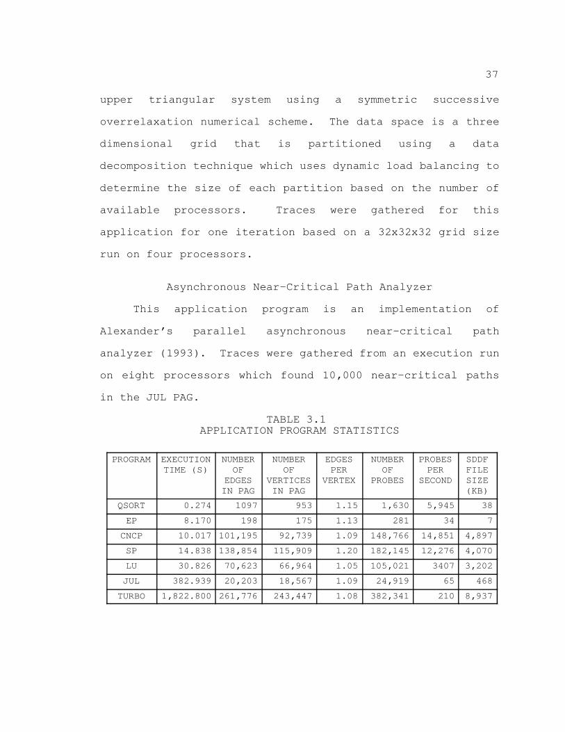
Table 3.1 presents a summary of application program

statistics.

Lower–Upper Solver

The Lower–Upper (LU) diagonal application benchmark

(Bailey et al. 1991) solves a regular–sparse block lower and

37

upper triangular system using a symmetric successive

overrelaxation numerical scheme. The data space is a three

dimensional grid that is partitioned using a data

decomposition technique which uses dynamic load balancing to

determine the size of each partition based on the number of

available processors. Traces were gathered for this

application for one iteration based on a 32x32x32 grid size

run on four processors.

Asynchronous Near–Critical Path Analyzer

This application program is an implementation of

Alexander’s parallel asynchronous near–critical path

analyzer (1993). Traces were gathered from an execution run

on eight processors which found 10,000 near–critical paths

in the JUL PAG.

TABLE 3.1 APPLICATION PROGRAM STATISTICS

PROGRAM EXECUTIONTIME (S)

NUMBEROF

EDGESIN PAG

NUMBEROF

VERTICESIN PAG

EDGESPER

VERTEX

NUMBEROF

PROBES

PROBESPER

SECOND

SDDFFILESIZE(KB)

QSORT 0.274 1097 953 1.15 1,630 5,945 38

EP 8.170 198 175 1.13 281 34 7

CNCP 10.017 101,195 92,739 1.09 148,766 14,851 4,897

SP 14.838 138,854 115,909 1.20 182,145 12,276 4,070

LU 30.826 70,623 66,964 1.05 105,021 3407 3,202

JUL 382.939 20,203 18,567 1.09 24,919 65 468

TURBO 1,822.800 261,776 243,447 1.08 382,341 210 8,937

38

Maximum Benefit Metric Calculation

An implementation of Alexander’s sequential BFS

near–critical path algorithm (1993) was extended to provide

for the calculation of critical and near–critical path

statistics. The original version generated a list of all

the critical and near–critical paths. Each path consisted

of a list of edge numbers. Code was developed which matched

edge numbers in each path with the corresponding edge

records so that the edge durations could be attributed to

the responsible application program components.

Calculation

Prior to receiving the edge numbers which appear on the

critical path, the oofi file is parsed and the edge file is

read. Object identifiers, operator identifiers, and

operator names are obtained, and each operator is assigned a

unique index value. For operator execution, message send,

and send overhead edges, a 2–dimensional array is allocated

to total edge times for each operator on each node. For

receive overhead edges, a vector is allocated to total edge

times for each node. When a critical path edge is found,

the edge type is determined, and the appropriate array or

vector is updated by adding the edge duration to the current

cell value.

When all of the edges on the critical path have been

found, two new sets of vectors are allocated for Maximum

39

Benefit calculation. One set is used to store the minimum

values across all near–critical paths, and the other is used

to collect times for each near–critical path that is

generated. While critical path information for each node

can provide useful load balancing information, such

information is contrary to the definition of the Maximum

Benefit metric. Therefore, before any near–critical path

edges are generated, the critical path arrays and vector are

summed across all nodes, resulting in three vectors and a

scalar value. The three vectors are used to collect

operator information for operator execution, message send,

and send overhead edge types. The scalar value is used to

collect information for the receive overhead edge type.

Upon reception of a near–critical path, the type of each

edge is determined, and the appropriate vector or scalar

value is updated. When every edge in the near–critical path

has been processed, the results contained in the set of

near–critical path values are compared to the set of minimum

values.

The difference in the length of the critical path and

this near–critical path, or the path slack, is added to all

values in the set of near–critical path data. Each value in

the set of near–critical path data is then compared to the

corresponding value in the minimum set of data. Should a

value be less than the minimum value, the minimum value is

updated. Before the values for the next near–critical path

40

are calculated, the set of near–critical path values is

zeroed. When all near–critical paths have been found and

processed, the minimum set of values contains the Maximum

Benefit metric values for every operator for each edge type.

Presentation

Critical and near–critical path data is presented in

tabular form. For critical path information, the output

consists of information presented on an edge type per node

basis, followed by a summary of edge types across all nodes.

Also, critical path information is broken down on an

operator per node basis, followed by a summary of operator

data across all nodes.

Near–critical path information is expressed in terms of

the Maximum Benefit metric for each operator broken down by

edge type, followed by a total of computation and

communication times across the entire program.

What If Scenario

Prior to implementing the What If scenarios code, only

the graph file contained the duration of edges. The edge

file contained only the original begin and end timestamps

from which the edge duration was obtained. In order to

simplify updating the duration of an edge and to avoid

manipulating timestamp data, a duration field was added to

each edge record in the edge file.

41

When performing What If analysis, the user is given a

choice of operators on which to simulate optimization based

on the content of the object information (oofi) file. A

specific operator is chosen, and the appropriate class

identifier and operator identifier is obtained. When an

optimization percentage is entered, the What If analyzer

steps through the graph and edge files, updating the

duration of the operator execution edges which correspond to

the chosen operator in both files. A new graph file and a

new edge file are generated. The new files can then be run

back through the near–critical path analyzer in order to

observe the effect that the simulated optimization had upon

the PAG and, in particular, the duration of the critical

path.

Pablo Module Development

During near–critical path analysis, those edges which

appear on any near–critical path are marked via a critical

path and near–critical path count field. Upon completion of

near–critical path analysis, marked edges are output in SDDF

records in order, sorted by timestamp. The Pablo

Performance Analysis Environment may then be used to

visualize the dynamic aspects of when events occurred during

execution. Although Pablo contains several display modules

for visualizing performance data, new modules were

constructed and added to Pablo to aid in visualizing

42

near–critical path data specifically. The two new modules

constructed were a labeled multi–bargraph module and a

string printer module.

Labeled Multi–Bargraph

Pablo contains a bargraph display module which displays

information from scalar, vector, and matrix input ports.

This display was initially used in visualizing near–critical

path data, and proved to be effective (Alexander 1993).

However, there are many limitations to the default bargraph

display module which needed to be improved upon. For

example, related data had to be distributed among several

different bargraph modules. In order to examine computation

and communication data for all nodes, the communication

bargraph had to be separate from the computation bargraph.

In a situation where a side–by–side comparison for each node

would be desirable, the default Pablo bargraph has no such

capabilities. Also, each bargraph display has only x–axis

and y–axis labels, regardless of how many bargraphs are

contained in each display. Meaningful labels are an

important part of any effective performance visualization

(Miller 1993). The new multi–bargraph display module

provides the capability to group related data and give a

label to each group and unique color to each bargraph in a

group. The Pablo bargraph display uses one color for all

43

bargraphs. A key is provided by the multi–bargraph so that

each colored bargraph can be given a descriptive label also.

String Printer

In cases where scalability for a display is crucial,

tables of information have proven to be inherently scalable

(Miller 1993). However, Pablo currently has no modules

which simply display text output. The string printer

display module displays character string input and can be

used to display tabular information. In cases where summary

statistics, such as those provided by IPS–2, are desirable,

the string printer can be used to convey such information.

Metric Comparison

Assessing the quality of the guidance given by a

profiling metric has proven to be a difficult task. One

technique utilized to quantitatively compare metrics is

called True Zeroing (Hollingsworth and Miller, 1992). True

Zeroing is similar to Logical Zeroing, but instead of

removing a procedure from a PAG, the procedure is actually

removed from the source code. Logical Zeroing was thought

to be an ineffective method of comparing metrics because

removing a procedure from a PAG wouldn’t reflect the actual

removing of the procedure from the source code. Due to

explicit parallel constructs such as semaphores and

barriers, Logical Zeroing could not reflect the substantial

re–ordering of events that would occur upon procedure

44

removal. Therefore, to accurately determine the result of

optimization and to determine the result of the metric

comparison, source code modifications were made.

Considerable effort was put into removing procedures from a

parallel program without affecting the end result.

The technique for metric comparison used in this study

is to utilize the What If scenarios to simulate the

optimization of OOF operators. The only synchronization

capability that OOF provides allows the programmer to

determine the order in which an object’s operators are

called. There are no explicit synchronization constructs,

and since the ordering of operators is maintained in What If

analysis, there should not be a substantial difference

between a modified PAG and a modified OOF program.

Therefore, in the cases where the ranking of operators by

CPM and MBM differ, What If analysis will be used to

simulate optimization of operators. The metric which gives

the best guidance is the metric whose simulated optimization

reduces the critical path duration, or total program

execution time, by the greatest amount.

45

CHAPTER IV

RESULTS

This chapter contains the results obtained from the

prototype implementation of the near–critical path analysis

framework. Maximum Benefit and Critical Path metric

calculations are presented and analyzed for each

application, and the results and applicability of the What

If scenarios and the Pablo visualization capabilities of the

framework are discussed.

Maximum Benefit Metric

The Maximum Benefit metric was calculated for each

application PAG at intervals of one, ten, one hundred, one

thousand, ten thousand, and one hundred thousand paths.

Recall that the Critical Path metric is identical to the

Maximum Benefit metric for one path. Operators are listed

in ranked order according to the value of the CPM.

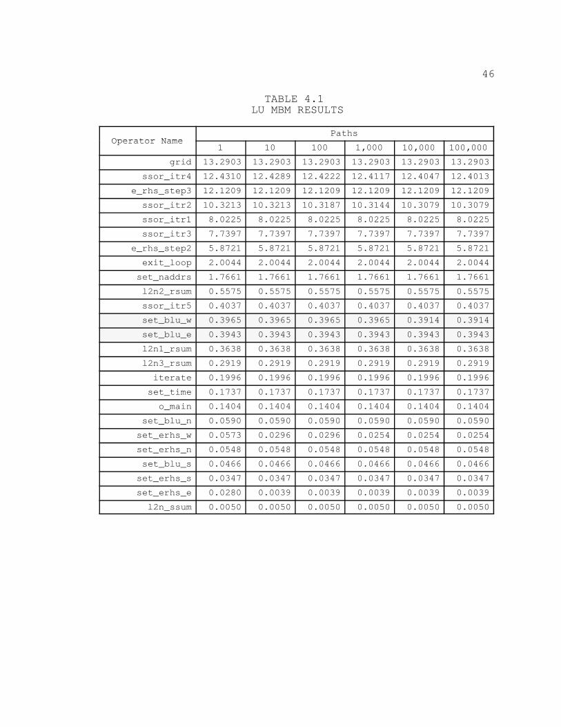
LU Results

Table 4.1 contains the MBM calculations for the LU

application. The results for the CPM and MBM do not differ

significantly for most of the operators. In fact, as the

number of near–critical paths traversed increases, the MBM

remains fairly constant for all operators.

46

TABLE 4.1 LU MBM RESULTS

Operator NamePaths

Operator Name1 10 100 1,000 10,000 100,000

grid 13.2903 13.2903 13.2903 13.2903 13.2903 13.2903

ssor_itr4 12.4310 12.4289 12.4222 12.4117 12.4047 12.4013

e_rhs_step3 12.1209 12.1209 12.1209 12.1209 12.1209 12.1209

ssor_itr2 10.3213 10.3213 10.3187 10.3144 10.3079 10.3079

ssor_itr1 8.0225 8.0225 8.0225 8.0225 8.0225 8.0225

ssor_itr3 7.7397 7.7397 7.7397 7.7397 7.7397 7.7397

e_rhs_step2 5.8721 5.8721 5.8721 5.8721 5.8721 5.8721

exit_loop 2.0044 2.0044 2.0044 2.0044 2.0044 2.0044

set_naddrs 1.7661 1.7661 1.7661 1.7661 1.7661 1.7661

l2n2_rsum 0.5575 0.5575 0.5575 0.5575 0.5575 0.5575

ssor_itr5 0.4037 0.4037 0.4037 0.4037 0.4037 0.4037

set_blu_w 0.3965 0.3965 0.3965 0.3965 0.3914 0.3914

set_blu_e 0.3943 0.3943 0.3943 0.3943 0.3943 0.3943

l2n1_rsum 0.3638 0.3638 0.3638 0.3638 0.3638 0.3638

l2n3_rsum 0.2919 0.2919 0.2919 0.2919 0.2919 0.2919

iterate 0.1996 0.1996 0.1996 0.1996 0.1996 0.1996

set_time 0.1737 0.1737 0.1737 0.1737 0.1737 0.1737

o_main 0.1404 0.1404 0.1404 0.1404 0.1404 0.1404

set_blu_n 0.0590 0.0590 0.0590 0.0590 0.0590 0.0590

set_erhs_w 0.0573 0.0296 0.0296 0.0254 0.0254 0.0254

set_erhs_n 0.0548 0.0548 0.0548 0.0548 0.0548 0.0548

set_blu_s 0.0466 0.0466 0.0466 0.0466 0.0466 0.0466

set_erhs_s 0.0347 0.0347 0.0347 0.0347 0.0347 0.0347

set_erhs_e 0.0280 0.0039 0.0039 0.0039 0.0039 0.0039

l2n_ssum 0.0050 0.0050 0.0050 0.0050 0.0050 0.0050

47

Rows 12 and 13 of the table have been shaded to

highlight an instance where the CPM and MBM differ. The CPM

ranks the set_blu_w operator ahead of the set_blu_e

operator, while the MBM has this order reversed.

CNCP Results

Table 4.2 contains the results of MBM calculation for

the CNCP application. No difference in the ranking of

operators between CPM and MBM is present for this PAG.

There does, however, appear to be a slow rate of descent in

the MBM for the first 2 operators. For this PAG, the

duration of the shortest near–critical path is still within

1 percent of the critical path duration. This descent may

suggest that as more near–critical paths are traversed, the

MBM may continue to decrease to a point where the ncp

operator, which appears to maintain a consistent MBM value,

could overtake reportNcPaths and traversePath in the

rankings.

JUL Results

Table 4.3 contains the results of the MBM calculation

for the JUL application. No significant difference in the

MBM and CPM values is present for the operators in this PAG.

Many similarities exist between the results of the previous

PAG and the results of this PAG. The duration of shortest

near–critical path for this PAG is within 1 percent of the

duration of the critical path, and a slow descent in the

48

value of the MBM for the nextcyc operator exists. However,

due to the significant difference in the MBM for nextcyc and

all other operators, the traversal of more near–critical

paths would probably have no effect upon MBM values.

EP Results


the EP application. No difference in the MBM and CPM

calculations exists for this PAG. The duration of the

shortest near–critical path is 97 percent of the critical

path duration. Traversing more near–critical paths would

undoubtedly have no effect on the values of the MBM for this

application, which is dominated by the grid operator.

SP Results


the SP application. No significant difference is present

between MBM and CPM calculations for this PAG. The duration

of the shortest near–critical path is within 1 percent of

the critical path duration. This PAG also contains

operators for which the MBM remains constant, and operators

for which the MBM seems to decrease steadily. Since the

distribution of the MBM is more even in this PAG, the

traversal of more near–critical paths would most likely

influence the ranking of the operators.

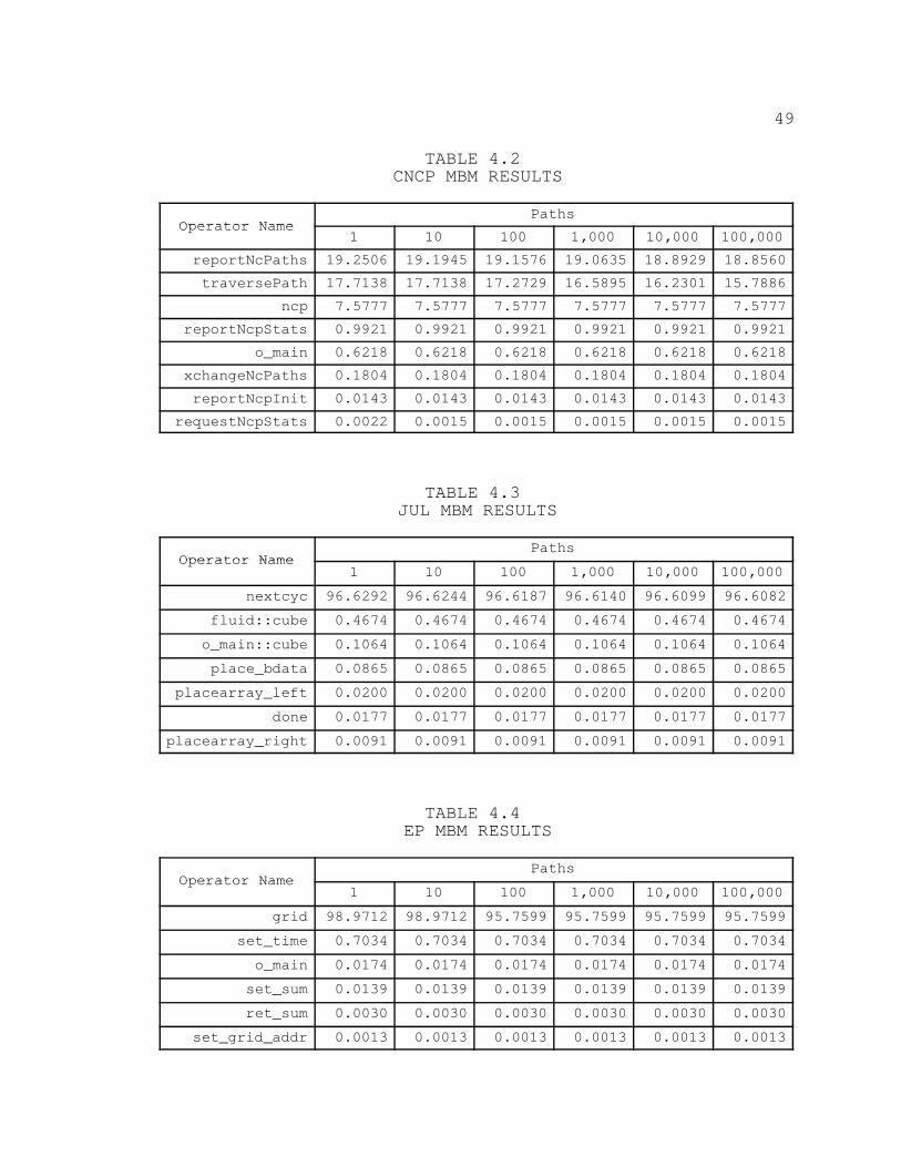
49

TABLE 4.2 CNCP MBM RESULTS

Operator NamePaths

Operator Name1 10 100 1,000 10,000 100,000

reportNcPaths 19.2506 19.1945 19.1576 19.0635 18.8929 18.8560

traversePath 17.7138 17.7138 17.2729 16.5895 16.2301 15.7886

ncp 7.5777 7.5777 7.5777 7.5777 7.5777 7.5777

reportNcpStats 0.9921 0.9921 0.9921 0.9921 0.9921 0.9921

o_main 0.6218 0.6218 0.6218 0.6218 0.6218 0.6218

xchangeNcPaths 0.1804 0.1804 0.1804 0.1804 0.1804 0.1804

reportNcpInit 0.0143 0.0143 0.0143 0.0143 0.0143 0.0143

requestNcpStats 0.0022 0.0015 0.0015 0.0015 0.0015 0.0015

TABLE 4.3 JUL MBM RESULTS

Operator NamePaths

Operator Name1 10 100 1,000 10,000 100,000

nextcyc 96.6292 96.6244 96.6187 96.6140 96.6099 96.6082

fluid::cube 0.4674 0.4674 0.4674 0.4674 0.4674 0.4674

o_main::cube 0.1064 0.1064 0.1064 0.1064 0.1064 0.1064

place_bdata 0.0865 0.0865 0.0865 0.0865 0.0865 0.0865

placearray_left 0.0200 0.0200 0.0200 0.0200 0.0200 0.0200

done 0.0177 0.0177 0.0177 0.0177 0.0177 0.0177

placearray_right 0.0091 0.0091 0.0091 0.0091 0.0091 0.0091

TABLE 4.4 EP MBM RESULTS

Operator NamePaths

Operator Name1 10 100 1,000 10,000 100,000

grid 98.9712 98.9712 95.7599 95.7599 95.7599 95.7599

set_time 0.7034 0.7034 0.7034 0.7034 0.7034 0.7034

o_main 0.0174 0.0174 0.0174 0.0174 0.0174 0.0174

set_sum 0.0139 0.0139 0.0139 0.0139 0.0139 0.0139

ret_sum 0.0030 0.0030 0.0030 0.0030 0.0030 0.0030

set_grid_addr 0.0013 0.0013 0.0013 0.0013 0.0013 0.0013

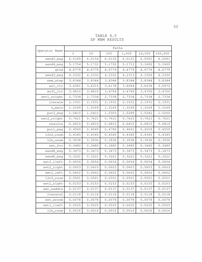
50

TABLE 4.5 SP MBM RESULTS

Operator NamePaths

Operator Name1 10 100 1,000 10,000 100,000

send5_msg 6.0189 6.0154 6.0125 6.0121 6.0091 6.0091

send4_msg 5.1754 5.1731 5.1730 5.1713 5.1682 5.1660

grid 4.6779 4.6779 4.6779 4.6779 4.6779 4.6779

send3_msg 4.2332 4.2332 4.2332 4.2313 4.2300 4.2300

new_step 3.8344 3.8344 3.8344 3.8344 3.8344 3.8344

xs1_itr 3.6281 3.6215 3.6178 3.6094 3.6039 3.5972

xs31_itr 3.4810 3.4810 3.4794 3.4769 3.4750 3.4750

set1_rright 2.7334 2.7334 2.7334 2.7334 2.7334 2.7334

iterate 2.1931 2.1931 2.1931 2.1931 2.1931 2.1931

o_main 1.3169 1.3169 1.3169 1.3169 1.3169 1.3169

put2_msg 1.0410 1.0410 1.0303 1.0289 1.0242 1.0200

set2_rright 0.7621 0.7621 0.7621 0.7621 0.7621 0.7621

results 0.6810 0.6810 0.6810 0.6810 0.6810 0.6810

put1_msg 0.4949 0.4949 0.4786 0.4691 0.4559 0.4559

l2n2_rsum 0.4345 0.4345 0.4345 0.4345 0.4345 0.4345

l2n_ssum 0.3938 0.3936 0.3936 0.3936 0.3936 0.3936

set_frc 0.3480 0.3480 0.3480 0.3480 0.3480 0.3480

send8_msg 0.3473 0.3473 0.3473 0.3473 0.3473 0.3473

send6_msg 0.3221 0.3221 0.3221 0.3221 0.3221 0.3221

set2_lleft 0.0654 0.0654 0.0654 0.0654 0.0654 0.0654

set2_right 0.0603 0.0603 0.0603 0.0603 0.0603 0.0603

set2_left 0.0602 0.0602 0.0602 0.0602 0.0602 0.0602

l2n3_rsum 0.0501 0.0501 0.0501 0.0501 0.0501 0.0501

set1_right 0.0153 0.0153 0.0153 0.0153 0.0153 0.0153

set_naddrs 0.0137 0.0137 0.0137 0.0137 0.0137 0.0137

iterate2 0.0118 0.0118 0.0118 0.0118 0.0118 0.0118

set_errnm 0.0078 0.0078 0.0078 0.0078 0.0078 0.0078

set1_lleft 0.0025 0.0025 0.0025 0.0025 0.0025 0.0025

l2n_rsum 0.0016 0.0016 0.0016 0.0016 0.0016 0.0016

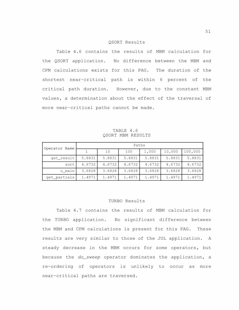
51

QSORT Results


the QSORT application. No difference between the MBM and

CPM calculations exists for this PAG. The duration of the

shortest near–critical path is within 6 percent of the

critical path duration. However, due to the constant MBM

values, a determination about the effect of the traversal of

more near–critical paths cannot be made.

TABLE 4.6 QSORT MBM RESULTS

Operator NamePaths

Operator Name1 10 100 1,000 10,000 100,000

get_result 5.8831 5.8831 5.8831 5.8831 5.8831 5.8831

sort 4.6732 4.6732 4.6732 4.6732 4.6732 4.6732

o_main 3.6828 3.6828 3.6828 3.6828 3.6828 3.6828

get_partials 1.4971 1.4971 1.4971 1.4971 1.4971 1.4971

TURBO Results


the TURBO application. No significant difference between

the MBM and CPM calculations is present for this PAG. These

results are very similar to those of the JUL application. A

steady decrease in the MBM occurs for some operators, but

because the do_sweep operator dominates the application, a

re–ordering of operators is unlikely to occur as more

near–critical paths are traversed.

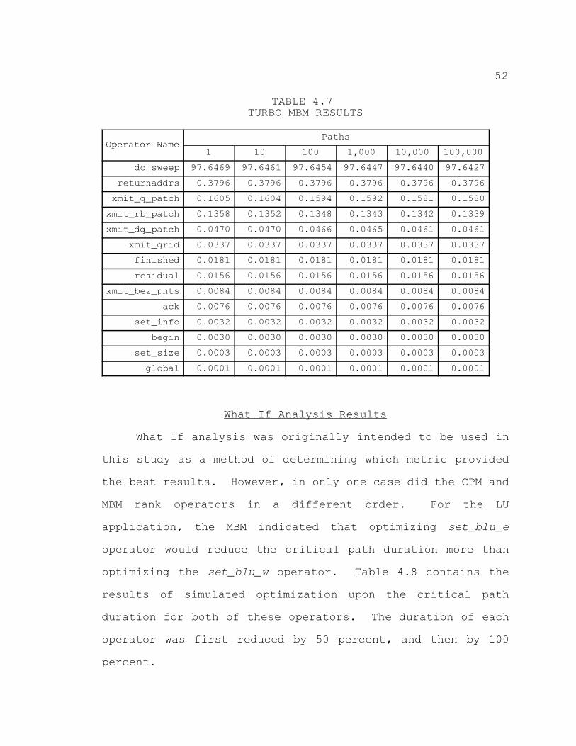
52

TABLE 4.7 TURBO MBM RESULTS

Operator NamePaths

Operator Name1 10 100 1,000 10,000 100,000

do_sweep 97.6469 97.6461 97.6454 97.6447 97.6440 97.6427

returnaddrs 0.3796 0.3796 0.3796 0.3796 0.3796 0.3796

xmit_q_patch 0.1605 0.1604 0.1594 0.1592 0.1581 0.1580

xmit_rb_patch 0.1358 0.1352 0.1348 0.1343 0.1342 0.1339

xmit_dq_patch 0.0470 0.0470 0.0466 0.0465 0.0461 0.0461

xmit_grid 0.0337 0.0337 0.0337 0.0337 0.0337 0.0337

finished 0.0181 0.0181 0.0181 0.0181 0.0181 0.0181

residual 0.0156 0.0156 0.0156 0.0156 0.0156 0.0156

xmit_bez_pnts 0.0084 0.0084 0.0084 0.0084 0.0084 0.0084

ack 0.0076 0.0076 0.0076 0.0076 0.0076 0.0076

set_info 0.0032 0.0032 0.0032 0.0032 0.0032 0.0032

begin 0.0030 0.0030 0.0030 0.0030 0.0030 0.0030

set_size 0.0003 0.0003 0.0003 0.0003 0.0003 0.0003

global 0.0001 0.0001 0.0001 0.0001 0.0001 0.0001

What If Analysis Results

What If analysis was originally intended to be used in

this study as a method of determining which metric provided

the best results. However, in only one case did the CPM and

MBM rank operators in a different order. For the LU

application, the MBM indicated that optimizing set_blu_e

operator would reduce the critical path duration more than

optimizing the set_blu_w operator. Table 4.8 contains the

results of simulated optimization upon the critical path

duration for both of these operators. The duration of each

operator was first reduced by 50 percent, and then by 100

percent.

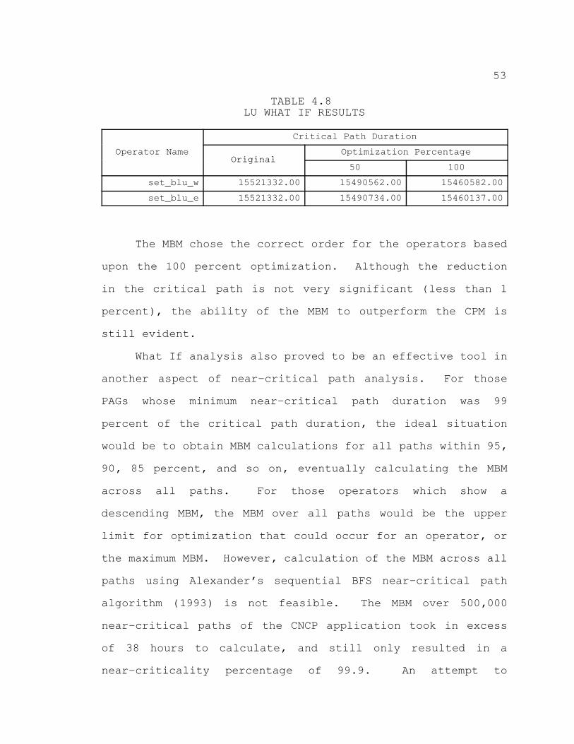
53

TABLE 4.8 LU WHAT IF RESULTS

Operator Name

Critical Path Duration

Operator NameOriginal

Optimization PercentageOperator NameOriginal

50 100

set_blu_w 15521332.00 15490562.00 15460582.00

set_blu_e 15521332.00 15490734.00 15460137.00

The MBM chose the correct order for the operators based

upon the 100 percent optimization. Although the reduction

in the critical path is not very significant (less than 1

percent), the ability of the MBM to outperform the CPM is

still evident.

What If analysis also proved to be an effective tool in

another aspect of near–critical path analysis. For those

PAGs whose minimum near–critical path duration was 99

percent of the critical path duration, the ideal situation

would be to obtain MBM calculations for all paths within 95,

90, 85 percent, and so on, eventually calculating the MBM

across all paths. For those operators which show a

descending MBM, the MBM over all paths would be the upper

limit for optimization that could occur for an operator, or

the maximum MBM. However, calculation of the MBM across all

paths using Alexander’s sequential BFS near–critical path

algorithm (1993) is not feasible. The MBM over 500,000

near–critical paths of the CNCP application took in excess

of 38 hours to calculate, and still only resulted in a

near–criticality percentage of 99.9. An attempt to

54

calculate the MBM across 1,000,000 paths was made, but the

analyzer ran as the only job on a Sun SPARCStation 10 for

more than a week without completing. Modification of an

implementation of Alexander’s synchronous parallel

near–critical path algorithm (1993) to include MBM

calculation was considered before arriving at a better means

of calculating the MBM across all paths.

Zeroing the duration of an operator in the PAG and

recalculating the critical path can show the true maximum

benefit that may be gained by optimizing that particular

operator across all paths. Therefore, the MBM for activity

i over all paths may be computed as follows:

MBMall(i) = ( 1 – ( d(i0)cp / dcp ) ) * 100.0

where d(i0)cp is the duration of the critical path with

activity i zeroed and dcp is the original critical path

duration.

What If analysis provides the capability to calculate

the MBM over all paths for all operators in minimal time

when compared to the sequential near–critical path analyzer.

For most applications, the time needed to find the original

critical path duration plus the time needed to update the

PAG and recalculate the new critical path duration for each

operator is comparable to the time needed to find 10,000

near–critical paths. The results of using this new method

of calculating the MBM for each application follow.

55

LU MBMall Results

Table 4.9 contains the results of CPM, MBM100,000, and

MBMall for the LU application. There is little difference

between the CPM and MBMall other than that which MBM100,000

has already revealed.

CNCP MBMall Results

Table 4.10 contains the results of MBMall calculation

together with the CPM and the MBM100,000 for the CNCP

application. A significant difference exists between not

only the CPM and the MBMall numbers, but also between MBMall

and MBM100,000. As was suspected, the descent of the MBM

continued as all near–critical paths were considered.

Clearly, the MBM reveals more characteristics of this

application than does the CPM.

JUL MBMall Results


for the JUL application. Very little difference in metric

values is present. As was expected, the consideration of

more near–critical paths had no significant effect upon the

MBM, due to the domination of nextcyc over all of the other

operators.

EP MBMall Results


for the EP application. This PAG is dominated by the grid

operator, resulting in the expected constant metric values.

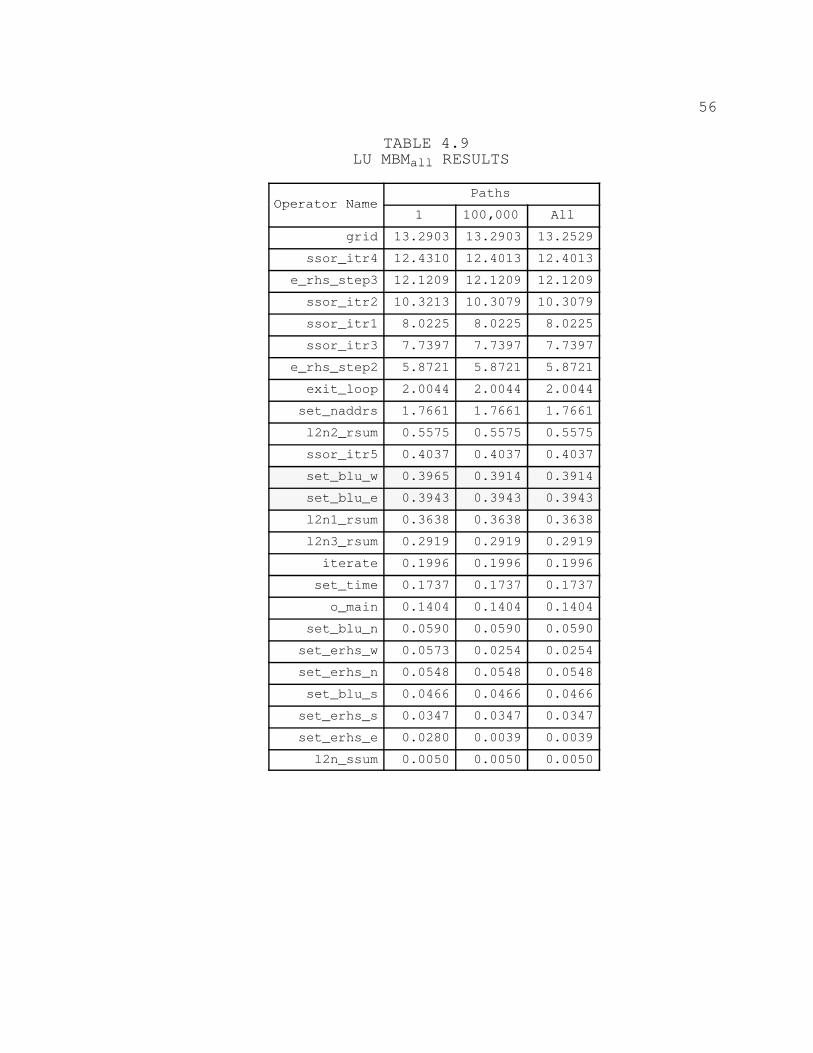
56

TABLE 4.9 LU MBMall RESULTS

Operator NamePaths

Operator Name1 100,000 All

grid 13.2903 13.2903 13.2529

ssor_itr4 12.4310 12.4013 12.4013

e_rhs_step3 12.1209 12.1209 12.1209

ssor_itr2 10.3213 10.3079 10.3079

ssor_itr1 8.0225 8.0225 8.0225

ssor_itr3 7.7397 7.7397 7.7397

e_rhs_step2 5.8721 5.8721 5.8721

exit_loop 2.0044 2.0044 2.0044

set_naddrs 1.7661 1.7661 1.7661

l2n2_rsum 0.5575 0.5575 0.5575

ssor_itr5 0.4037 0.4037 0.4037

set_blu_w 0.3965 0.3914 0.3914

set_blu_e 0.3943 0.3943 0.3943

l2n1_rsum 0.3638 0.3638 0.3638

l2n3_rsum 0.2919 0.2919 0.2919

iterate 0.1996 0.1996 0.1996

set_time 0.1737 0.1737 0.1737

o_main 0.1404 0.1404 0.1404

set_blu_n 0.0590 0.0590 0.0590

set_erhs_w 0.0573 0.0254 0.0254

set_erhs_n 0.0548 0.0548 0.0548

set_blu_s 0.0466 0.0466 0.0466

set_erhs_s 0.0347 0.0347 0.0347

set_erhs_e 0.0280 0.0039 0.0039

l2n_ssum 0.0050 0.0050 0.0050

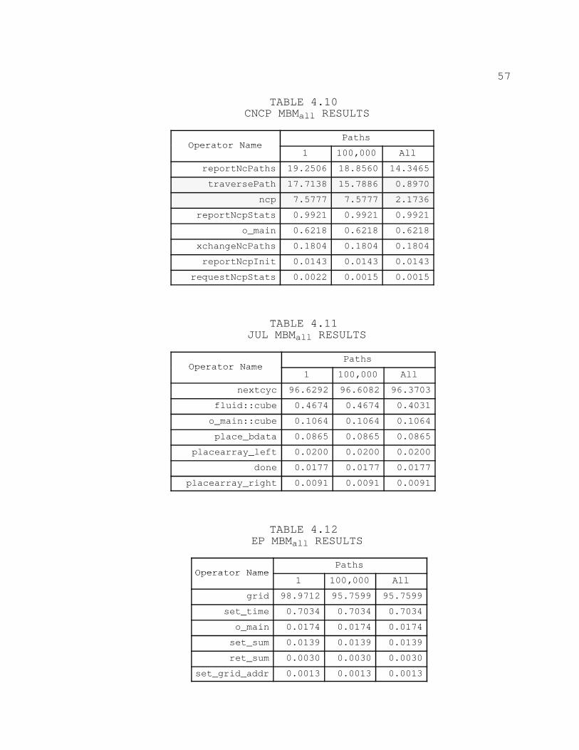
57

TABLE 4.10 CNCP MBMall RESULTS

Operator NamePaths


reportNcPaths 19.2506 18.8560 14.3465

traversePath 17.7138 15.7886 0.8970

ncp 7.5777 7.5777 2.1736

reportNcpStats 0.9921 0.9921 0.9921

o_main 0.6218 0.6218 0.6218

xchangeNcPaths 0.1804 0.1804 0.1804

reportNcpInit 0.0143 0.0143 0.0143

requestNcpStats 0.0022 0.0015 0.0015

TABLE 4.11 JUL MBMall RESULTS

Operator NamePaths


nextcyc 96.6292 96.6082 96.3703

fluid::cube 0.4674 0.4674 0.4031

o_main::cube 0.1064 0.1064 0.1064

place_bdata 0.0865 0.0865 0.0865

placearray_left 0.0200 0.0200 0.0200

done 0.0177 0.0177 0.0177

placearray_right 0.0091 0.0091 0.0091

TABLE 4.12 EP MBMall RESULTS

Operator NamePaths


grid 98.9712 95.7599 95.7599

set_time 0.7034 0.7034 0.7034

o_main 0.0174 0.0174 0.0174

set_sum 0.0139 0.0139 0.0139

ret_sum 0.0030 0.0030 0.0030

set_grid_addr 0.0013 0.0013 0.0013

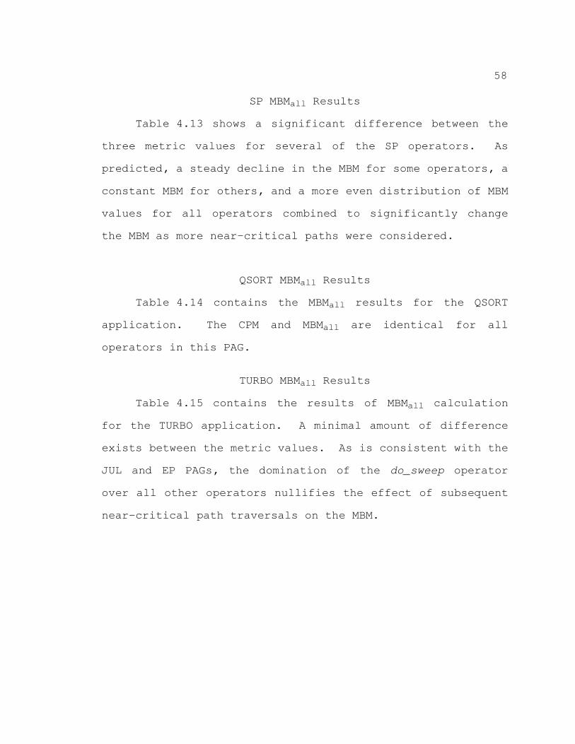
58

SP MBMall Results

Table 4.13 shows a significant difference between the

three metric values for several of the SP operators. As

predicted, a steady decline in the MBM for some operators, a

constant MBM for others, and a more even distribution of MBM

values for all operators combined to significantly change

the MBM as more near–critical paths were considered.

QSORT MBMall Results

Table 4.14 contains the MBMall results for the QSORT

application. The CPM and MBMall are identical for all

operators in this PAG.

TURBO MBMall Results


for the TURBO application. A minimal amount of difference

exists between the metric values. As is consistent with the

JUL and EP PAGs, the domination of the do_sweep operator

over all other operators nullifies the effect of subsequent

near–critical path traversals on the MBM.

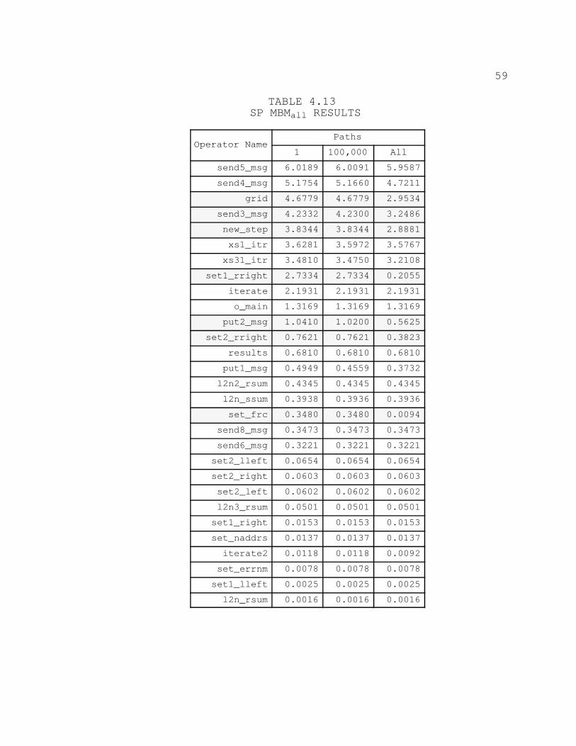
59

TABLE 4.13 SP MBMall RESULTS

Operator NamePaths


send5_msg 6.0189 6.0091 5.9587

send4_msg 5.1754 5.1660 4.7211

grid 4.6779 4.6779 2.9534

send3_msg 4.2332 4.2300 3.2486

new_step 3.8344 3.8344 2.8881

xs1_itr 3.6281 3.5972 3.5767

xs31_itr 3.4810 3.4750 3.2108

set1_rright 2.7334 2.7334 0.2055

iterate 2.1931 2.1931 2.1931

o_main 1.3169 1.3169 1.3169

put2_msg 1.0410 1.0200 0.5625

set2_rright 0.7621 0.7621 0.3823

results 0.6810 0.6810 0.6810

put1_msg 0.4949 0.4559 0.3732

l2n2_rsum 0.4345 0.4345 0.4345

l2n_ssum 0.3938 0.3936 0.3936

set_frc 0.3480 0.3480 0.0094

send8_msg 0.3473 0.3473 0.3473

send6_msg 0.3221 0.3221 0.3221

set2_lleft 0.0654 0.0654 0.0654

set2_right 0.0603 0.0603 0.0603

set2_left 0.0602 0.0602 0.0602

l2n3_rsum 0.0501 0.0501 0.0501

set1_right 0.0153 0.0153 0.0153

set_naddrs 0.0137 0.0137 0.0137

iterate2 0.0118 0.0118 0.0092

set_errnm 0.0078 0.0078 0.0078

set1_lleft 0.0025 0.0025 0.0025

l2n_rsum 0.0016 0.0016 0.0016

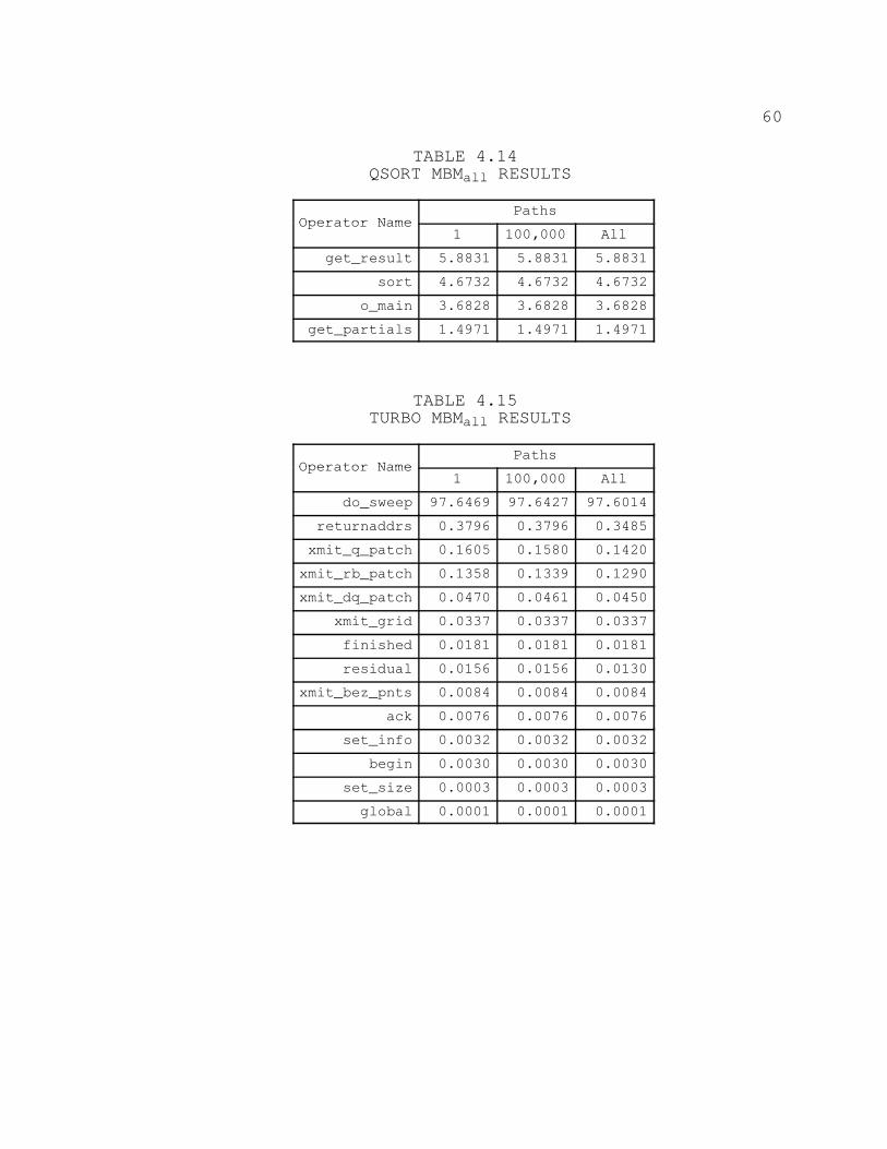
60

TABLE 4.14 QSORT MBMall RESULTS

Operator NamePaths


get_result 5.8831 5.8831 5.8831

sort 4.6732 4.6732 4.6732

o_main 3.6828 3.6828 3.6828

get_partials 1.4971 1.4971 1.4971

TABLE 4.15 TURBO MBMall RESULTS

Operator NamePaths


do_sweep 97.6469 97.6427 97.6014

returnaddrs 0.3796 0.3796 0.3485

xmit_q_patch 0.1605 0.1580 0.1420

xmit_rb_patch 0.1358 0.1339 0.1290

xmit_dq_patch 0.0470 0.0461 0.0450

xmit_grid 0.0337 0.0337 0.0337

finished 0.0181 0.0181 0.0181

residual 0.0156 0.0156 0.0130

xmit_bez_pnts 0.0084 0.0084 0.0084

ack 0.0076 0.0076 0.0076

set_info 0.0032 0.0032 0.0032

begin 0.0030 0.0030 0.0030

set_size 0.0003 0.0003 0.0003

global 0.0001 0.0001 0.0001

61

Visualization Results

Figure 4.1 contains an example of the new labeled

multi–bargraph display module which was developed for the

Pablo Performance Analysis Environment. In this example,

the critical path percentage is displayed for each operator

based on edge type. Each of the three bargraphs associated

with an operator label is given a unique color. The mapping

of color to edge type is displayed in a popup window when

the user pushes the “Key” button. An example of a key popup

is contained in Figure 4.2.

When the user clicks anywhere inside any of the

bargraphs in the display, all the values associated with

that specific bargraph are displayed in a popup window.

Clicking in the third bargraph of the first label of

Figure 4.1 results in the popup window shown in Figure 4.3.

Figure 4.4 shows another possible use of the new

multi–bargraph display module. In this example, the

critical path percentage, broken down by communication and

computation, is shown for each operator. Figure 4.5 and

Figure 4.6 contain the popups associated with this display.

This new display module can be used to show any two

dimensional relationship. For example, near–critical path

computation versus communication could be displayed for each

node. Likewise, the near–critical path duration for each

operator on each node could be displayed.

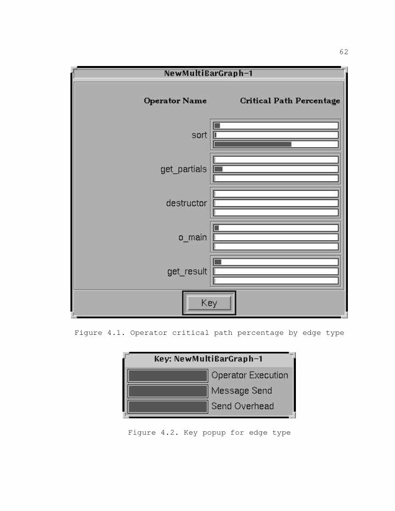
62

Figure 4.1. Operator critical path percentage by edge type

Figure 4.2. Key popup for edge type

63

Figure 4.3. Bargraph value popup

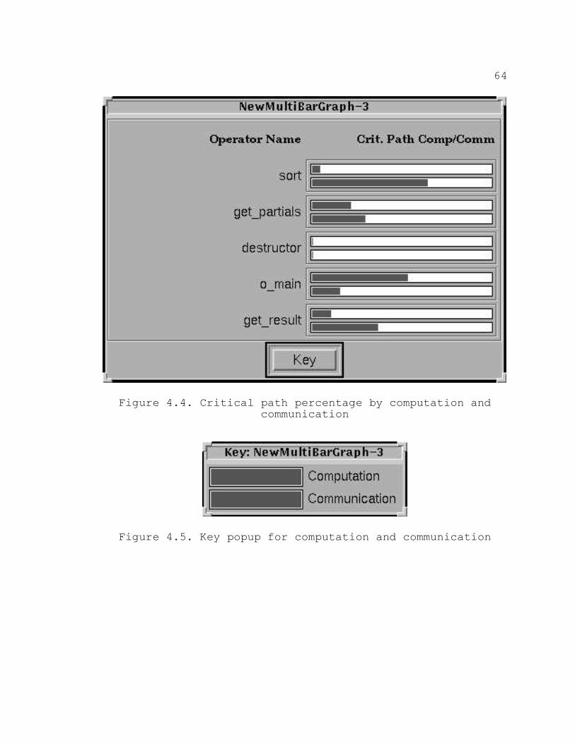
64

Figure 4.4. Critical path percentage by computation andcommunication

Figure 4.5. Key popup for computation and communication

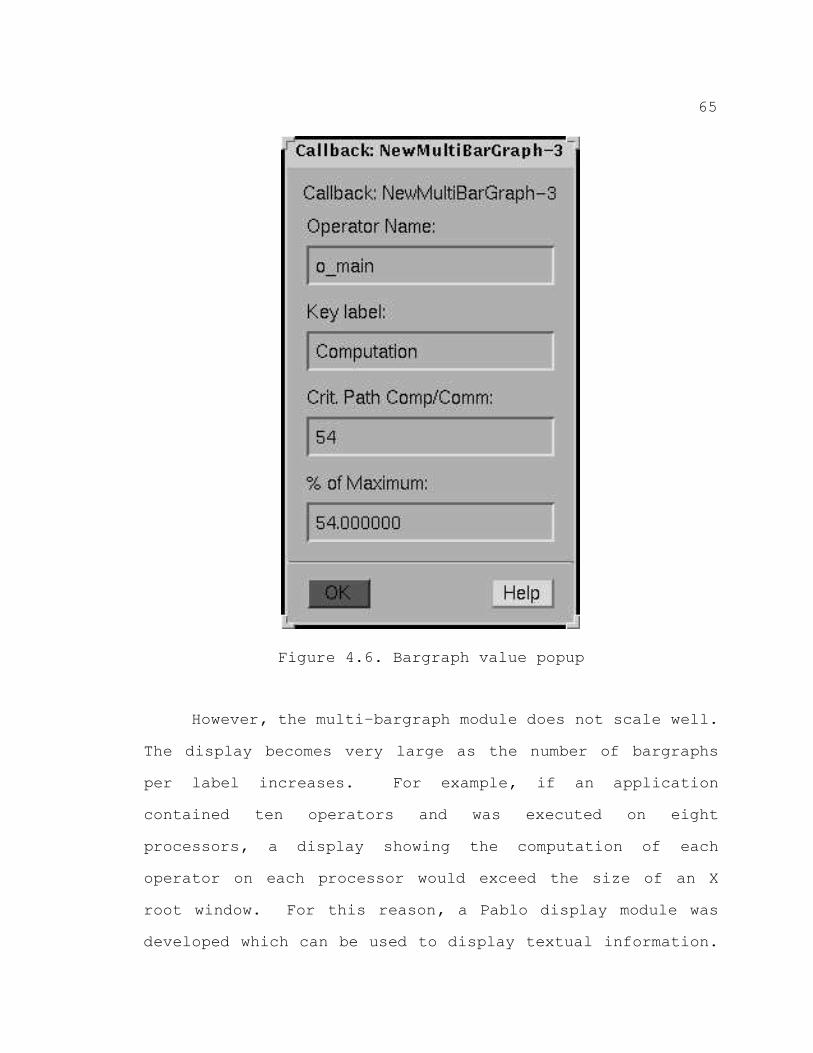
65

Figure 4.6. Bargraph value popup

However, the multi–bargraph module does not scale well.

The display becomes very large as the number of bargraphs

per label increases. For example, if an application

contained ten operators and was executed on eight

processors, a display showing the computation of each

operator on each processor would exceed the size of an X

root window. For this reason, a Pablo display module was

developed which can be used to display textual information.

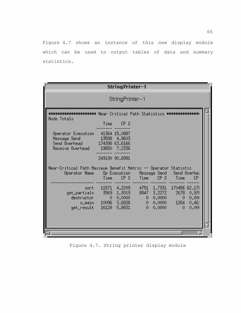
66

Figure 4.7 shows an instance of this new display module

which can be used to output tables of data and summary

statistics.

Figure 4.7. String printer display module

67

CHAPTER V

SUMMARY AND CONCLUSIONS

Summary

The main goal of this research was to investigate the

effectiveness of the Maximum Benefit metric(MBM) as a

guidance tool for parallel program performance debugging,

and to assess the ability of the MBM to provide the basis

for an additional set of performance monitoring tools. All

three perspectives of a previously proposed near–critical

path analysis framework were implemented and tested on

several application programs. Results from the statistical

component as well as the contingency and visualization

components of the framework were presented and discussed.

The quality and effectiveness of the guidance which the

MBM provides were tested using direct comparison between the

MBM and Critical Path metric(CPM) for all applications. The

contingency component, What If analysis, was to be utilized

to determine which metric provided the best information. By

simulating program optimization, What If analysis was

intended to be able to ascertain which metric’s guidance had

the greatest impact upon reducing an application’s critical

path duration, thereby reducing the total execution time.

68

However, due to the limited number of paths used in MBM

calculation, only one case existed where the MBM and CPM

provided differing guidance. Even though What If analysis

determined that the MBM had indeed provided better

direction, insufficient evidence was available to make any

conclusions about the utility of the MBM over the CPM.

In order to overcome the obstacle of using only a

limited number of paths to calculate the MBM, a new method

of computing the MBM across all paths was developed. This

new method uses What If scenarios to determine the

percentage of improvement which will be gained by zeroing

each program component. Although this method had been used

previously as a guidance tool, the results of each

improvement had never been directly attributed to specific

program components in this manner. This new method not only

reduced the amount of time required to calculate meaningful

MBM results, but also eliminated the need to use any

secondary means of effectiveness testing. The MBM across

all paths combines the computation of the MBM and the

testing of the metric’s guidance into one complete process.

The MBM over all paths was calculated for all

applications, and several instances where the MBM

outperformed the CPM were discovered.

Two Pablo display modules were developed as part of the

visualization component of the framework. A multi–purpose

bargraph display makes use of effective labeling and color

69

to visualize a wide variety of near–critical path data. The

new bargraph display can be used to dynamically display two

dimensional data relationships. A new textual display

module was developed that provides a means to view tables of

textual data which can be used for summary statistics and

instances when a more scalable visual display is desired.

Conclusions

The Maximum Benefit metric clearly reveals additional

characteristics about parallel program performance. Because

the MBM across all paths is the upper limit on the maximum

benefit that can be achieved by optimizing a particular

program component, and since the Critical Path metric is

simply the MBM over the critical path, the MBM will always

outperform the CPM. However, a detriment to performing MBM

calculation using What If analysis is the loss of the

ability to collect information about the edges which lie on

the near–critical paths. This information is vital to the

visualization component of the framework which has proven to

be a valuable tool. The Maximum Benefit metric, together

with contingency and visualization analysis, clearly

provides a sound basis for additional performance monitoring

tools.

Limitations

Several limitations were encountered while conducting

this research. All applications were implemented using the

70

Object–Oriented Fortran parallel programming environment.

OOF encourages algorithms which use domain decomposition to

partition the problem space and which use a limited amount

of communication between computing nodes. Several of the

applications used in this study have characteristics which

are typical of most OOF programs. One common trait is that

all nodes perform iterations of the same operations at

essentially the same time. Cycles of long periods of

computation followed by an exchange of data are common

occurrences. This pattern is then reflected in the

resulting PAG, and the possibility that the same sequence of

edges appears on all segments at some point in the PAG is

likely. Therefore, two near–critical paths may wind through

the graph without overlapping and still result in virtually

the same set of Maximum Benefit statistics. The application

which showed the most evidence of the utility of the MBM is

one in which nodes worked independently of one another. The

parallel near–critical path analyzer distributes partial

paths among the nodes, and each node works independently

traversing paths and reporting results back to a central

scheduler.

The use of the MSPARC multicomputer and the MSPARC

Instrumentation System limited the number of available

computing nodes to eight, and placed boundaries on the types

of probes which could be collected. For those applications

in which one operator does the majority of the work, the

71

ability to further break down the operator into

subcomponents might reveal additional hidden bottlenecks.

Future Research

Many areas of this study could be investigated further

to advance research into near–critical path analysis as a

parallel program performance debugging tool. Each component

of the near–critical path analysis framework has many

possible research paths to traverse.

The calculation of the MBM could be extended to provide

node–based information which could be useful in analyzing

load balancing. While communication MBM statistics were

calculated for all applications in this study, only the

computation results were examined. Communication statistics

could provide an indication of the appropriateness of the

interconnection network and other communication related

characteristics.

For systems which do not have implicit synchronization

capabilities, research into modification of existing program

activity graphs to simulate function optimization could

reveal additional techniques for contingency scenario

implementation. Shared memory constructs such as semaphores

and barriers introduce a variety of timing problems

associated with PAG manipulation. In cases where What If

implementation could not be utilized to calculate the MBM

72

across all paths, a parallel version of the near–critical

path analyzer could be modified to perform MBM calculation.

The aspect of the framework which provides the most

opportunities and would benefit the most from further

research is the visualization component. Virtual reality is

currently being investigated as a means for viewing

near–critical path data (Reed et al. 1994). Large numbers

of vertices and nodes which result in millions of possible

paths in a PAG make visualization of near–critical path

traversal a formidable task. Virtual reality seems to be

the most promising method which can be used to visually, and

possibly aurally, relate near–critical path data to the

application programmer.

73

REFERENCES

Alexander, Cedell A. 1993. Multicomputer performancemonitoring: A standards–based approach. MississippiState, Mississippi: National ScienceFoundation/Mississippi State University EngineeringResearch Center for Computational Field Simulation.Technical report MSSU–EIRS–93–13.

Alexander, Cedell A. 1994. Near–critical path algorithms forprogram activity graphs. Ph.D. diss., Mississippi StateUniversity.

Alexander, Cedell A., D. S. Reese, and J. C. Harden. 1994.Near–critical path analysis of program activity graphs.In Proceedings of the second international workshop onmodeling, analysis, and simulation of computer andtelecommunication systems in Durham, North Carolina,January 31–February 2, 1994, 308–17. Los Alamitos:IEEE Computer Society Press.

Anderson, Thomas E. and Edward D. Lazowska. 1990. Quartz: Atool for tuning parallel program performance. InProceedings of the 1990 SIGMETRICS conference onmeasurement and modeling of computer systems in Boston,Massachusetts, May, 1990, 115–25. New York:Association of Computing Machinery Press.

Aydt, Ruth A. 1992. The Pablo self–defining data format.Urbana–Champagne, Illinois: Department of ComputerScience, University of Illinois. Technical report.

Bailey, David H., J.T. Barton, T. Lesinski, and Horst D.Simon. 1991. The NAS parallel benchmarks. Moffet Field,California: NASA Ames Research Center. Technical reportRNR–91–002.

Geist, G. A., M. T. Heath, B. W. Peyton, and P. H. Worley.1992. A users’ guide to PICL: A portable instrumentedcommunication library. Oak Ridge, Tennessee: Oak RidgeNational Laboratory. Technical report ORNL/TM–11616.

74

Graham, S. L., P. B. Kessler, and M. K. McKusick. 1982.Gprof: A call graph execution profiler. In Proceedingsof the ACM SIGPLAN symposium on compiler constructionin Boston, Massachusetts, June, 1982, 120–26. NewYork: Association of Computing Machinery Press.

Harden, James, Donna Reese, Filip To, Dan Linder, ChrisBorchert, and Girault Jones. 1992. A performancemonitor for the MSPARC multicomputer. In Proceedings ofthe IEEE southeastcon ’92 in Birmingham, Alabama, April12–15, 1992, 724–29. Los Alamitos: IEEE ComputerSociety Press.

Heath, Michael T. and Jennifer A. Etheridge. 1991.Visualizing performance of parallel programs. OakRidge, Tennessee: Oak Ridge National Laboratory.Technical report ORNL/TM–11813.

Henley, Greg J. and J. Mark Janus. 1991. Parallelization andconvergence of a 3D implicit unsteady turbomachineryflow code. In Proceedings of the 5th SIAM conference onparallel processing for scientific computing inHouston, Texas, March 25–27, 1991, 238–45.Philadelphia: Society for Industrial and AppliedMathematics.

Herrarte, V. and Ewing Lusk. 1991. Studying parallelprogram behavior with Upshot. Argonne, Illinois:Mathematics and Computer Science Division, ArgonneNational Laboratory.

Hoare, C. A. R. 1962. Quicksort. Computer Journal 5 (May):10–15.

Hollingsworth, Jeffrey K. and Barton P. Miller. 1992.Parallel program performance metrics: A comparison andvalidation. In Proceedings of supercomputing ’92 inMinneapolis, Minnesota, November 16–20, 1992, 4–13. LosAlamitos: IEEE Computer Society Press.

Hollingsworth, Jeffrey K. and Barton P. Miller. 1993.Dynamic control of performance monitoring on largescale parallel systems. In Proceedings of the seventhACM international conference on supercomputing inTokyo, Japan, July 19–23, 1993, 185–94. New York:Association of Computing Machinery Press.

75

Kalé, Laxmikant V. 1990. The Chare kernel parallelprogramming language and system. In Proceedings of the1990 international conference on parallel processing inChicago, Illinois, August 13–17, 1990, II–17 – II–25.University Park: Pennsylvania State University Press.

Kohn, James and Winifred Williams. 1993. ATExpert. Journalof Parallel and Distributed Computing 18 (June):205–22.

Miller, Barton P. 1993. What to draw? When to draw? Anessay on parallel program visualization. Journal ofParallel and Distributed Computing 18 (June): 265–69.

Miller, Barton P., Morgan Clark, Jeff Hollingsworth, StevenKierstead, Sek–See Lim, and Timothy Torzewski. 1990.IPS–2: The second generation of a parallel programmeasurement system. IEEE Transactions on Parallel andDistributed Systems 1 (April): 206–17.

Reed, Daniel A., Ruth A. Aydt, Tara M. Madhyastha, Roger J.Noe, Keith A. Shields, and Bradley W. Schwartz. 1992.An overview of the Pablo performance analysisenvironment. Urbana–Champagne, Illinois: Department ofComputer Science, University of Illinois. Technicalreport.

Reed, Daniel A., Keith A. Shields, Will H. Scullin, Luis F.Tavera, and Christopher L. Elford. 1994. Virtualreality and parallel systems performance analysis.Mosaic URL http://bugle.cs.uiuc.edu/Papers/VR.ps.Z.

Reese, Donna S. and Edward A. Luke. 1991. Object orientedfortran for development of portable parallel programs.In Proceedings of the third IEEE symposium on paralleland distributed systems in Dallas, Texas, December 2–5,1991, 608–15. Los Alamitos: IEEE Computer SocietyPress.

Sinha, Amitabh B., and Laxmikant V. Kalé. 1993.Projections: A preliminary performance tool for Charm.Mosaic URL file://a.cs.uiuc.edu/pub/CHARM/papers/Projections_ ICPP_93.ps.

Sinha, Amitabh B., and Laxmikant V. Kalé. 1994. Aframework for intelligent performance feedback. MosaicURL file://a.cs.uiuc.edu/pub/CHARM/papers/Projections_ICPP_94.ps.

Sunderam, V. S. 1990. PVM: A framework for paralleldistributed computing. Concurrency: Practice andExperience 2 (December): 315–39.

76

Whitfield, David L. and J. Mark Janus. 1984. Threedimensional unsteady euler equations solutions usingflux vector splitting. In Seventeenth fluid dynamics,plasma dynamics, and lasers conference, AIAA–84–1552,June 25–27, 1984, by the American Institute ofAeronautics and Astronautics.

Yang, Cui–Qing and Barton P. Miller. 1989. Performancemeasurement of parallel and distributed programs: Astructural and automatic approach. IEEE Transactions onSoftware Engineering 15 (December): 1615–29.

Documents

NEAR–CRITICAL PATH ANALYSIS OF PARALLEL …rbbrigh/papers/R_Brightwell94.pdf · NEAR–CRITICAL PATH ANALYSIS OF PARALLEL PROGRAM PERFORMANCE: THE STATISTICAL PERSPECTIVE By Ronald