Embed Size (px)
Citation preview

1
Near Optimal Signal Recoveryfrom Random Projections
Emmanuel Candes, California Institute of Technology
Multiscale Geometric Analysis in High Dimensions: Workshop # 2IPAM, UCLA, October 2004
Collaborators : Justin Romberg (Caltech), Terence Tao (UCLA)
2
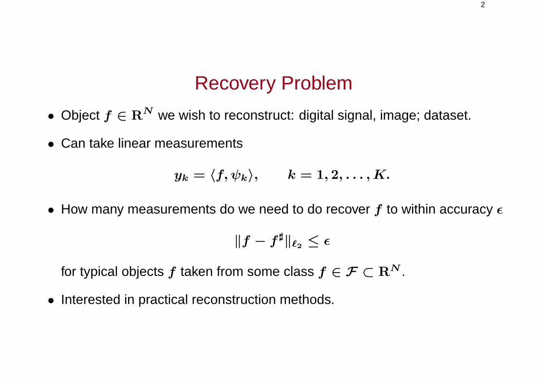
Recovery Problem
• Object f ∈ RN we wish to reconstruct: digital signal, image; dataset.
• Can take linear measurements
yk = 〈f, ψk〉, k = 1, 2, . . . ,K.
• How many measurements do we need to do recover f to within accuracy ε
‖f − f ]‖`2 ≤ ε
for typical objects f taken from some class f ∈ F ⊂ RN .
• Interested in practical reconstruction methods.

3
Agenda
• Background: exact reconstruction of sparse signals
• Near-optimal reconstruction of compressible signals
• Uniform uncertainty principles
• Exact reconstruction principles
• Relationship with coding theory
• Numerical experiments

4
Sparse Signals
• Vector f ∈ RN ; digital signal, coefficients of a digital signal/image, etc.)
• |T | nonzero coordinates (|T | spikes)
T := t, f(t) 6= 0
• Do not know the locations of the spikes
• Do not know the amplitude of the spikes

5
Recovery of Sparse Signals
• Sparse signal f : |T | spikes
• Available information
y = F f,
F is K by N with K << N
• Can we recover f from K measurements?

6
Fourier Ensemble
• Random set Ω ⊂ 0, . . . , N − 1, |Ω| = K.
• Random frequency measurements: observe (Ff)k = f(k)
f(k) =N−1∑t=0
f(t)e−i2πkt/N , k ∈ Ω

7
Exact Recovery from Random Frequency Samples
• Available information: yk = f(k), Ω random and |Ω| = K.
• To recover f , simply solve
(P1) f ] = argming∈RN ‖g‖`1 , subject to Fg = Ff.
where
‖g‖`1 :=N−1∑t=0
|g(t)|.
Theorem 1 (C., Romberg, Tao) Suppose
|K| ≥ α · |T | · logN.
Then the reconstruction is exact with prob. greater than 1 − O(N−αρ) forsome fixed ρ > 0: f ] = f . (N.b. ρ ≈ 1/29 works).

8
Exact Recovery from Gaussian Measurements
• Gaussian random matrix
F (k, t) = Xk,t, Xk,t i.i.d. N(0, 1)
• This will be called the Gaussian ensemble
Solve
(P1) f ] = argming∈RN ‖g‖`1 subject to Fg = Ff.
Theorem 2 (C., Tao) Suppose
|K| ≥ α · |T | · logN.
Then the reconstruction is exact with prob. greater than 1 − O(N−αρ) forsome fixed ρ > 0: f ] = f .

9
Gaussian Random Measurements
yk = 〈f,X〉, Xt i.i.d. N(0, 1)
0 50 100 150 200 250 300−0.2
−0.15
−0.1
−0.05
0
0.05
0.1
0.15
0.2Random basis element

10
Equivalence
• Combinatorial optimization problem
(P0) ming
‖g‖`0 := #t, g(t) 6= 0, F g = Ff
• Convex optimization problem (LP)
(P1) ming
‖g‖`1 , F g = Ff
• Equivalence:
For K |T | logN , the solutions to (P0) and (P1) are unique and are thesame!

11
About the `1-norm
• Minimum `1-norm reconstruction in widespread use
• Santosa and Symes (1986) proposed this rule to reconstruct spike trainsfrom incomplete data
• Connected with Total-Variation approaches, e.g. Rudin, Osher, Fatemi(1992)
• More recently, `1-minimization, Basis Pursuit, has been proposed as aconvex alternative to the combinatorial norm `0. Chen, Donoho Saunders(1996)
• Relationships with uncertainty principles: Donoho & Huo (01), Gribonval &Nielsen (03), Tropp (03) and (04), Donoho & Elad (03)

12
min `1 as LP
min ‖x‖`1 subject to Ax = b
• Reformulated as an LP (at least since the 50’s).
• Split x into x = x+ − x−
min 1Tx+ + 1Tx− subject to
(A −A
) x+
x−
= b
x+ ≥ 0, x− ≥ 0

13
Reconstruction of Spike Trains from Fourier Samples
• Gilbert et al. (04)
• Santosa & Symes (86)
• Dobson & Santosa (96)
• Bresler & Feng (96)
• Vetterli et. al. (03)
14
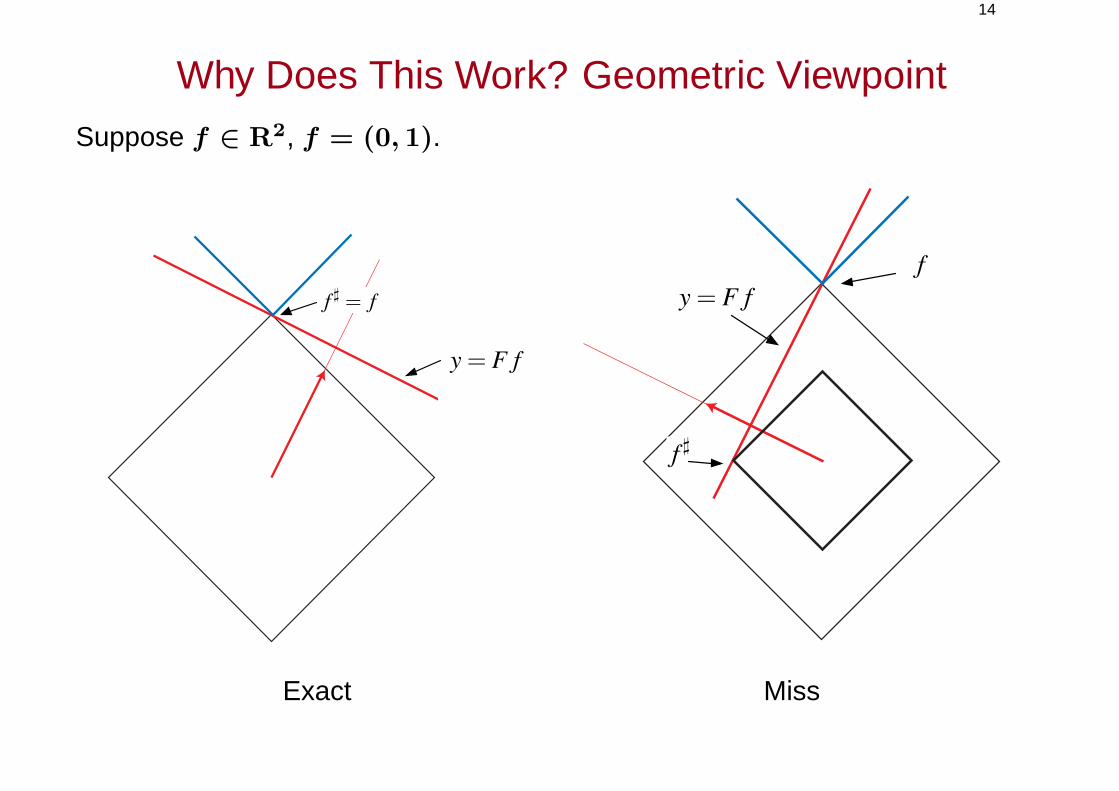
Why Does This Work? Geometric Viewpoint
Suppose f ∈ R2, f = (0, 1).
y= F f
f ! = f
f !
fy= F f
Exact Miss

15
Higher Dimensions

16
Duality in Linear/Convex Programming
• f unique solution ’if and only’ if dual is feasible
• Dual is feasible if there is P ∈ RN
– P is in the rowspace of F
– P is a subgradient of ‖f‖`1
P ∈ ∂‖f‖`1 ⇔
P (t) = sgn(f(t)), t ∈ T
|P (t)| < 1, t ∈ T c
17
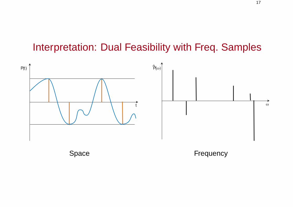
Interpretation: Dual Feasibility with Freq. Samples
t
P(t) P(!)
!
^
Space Frequency
18
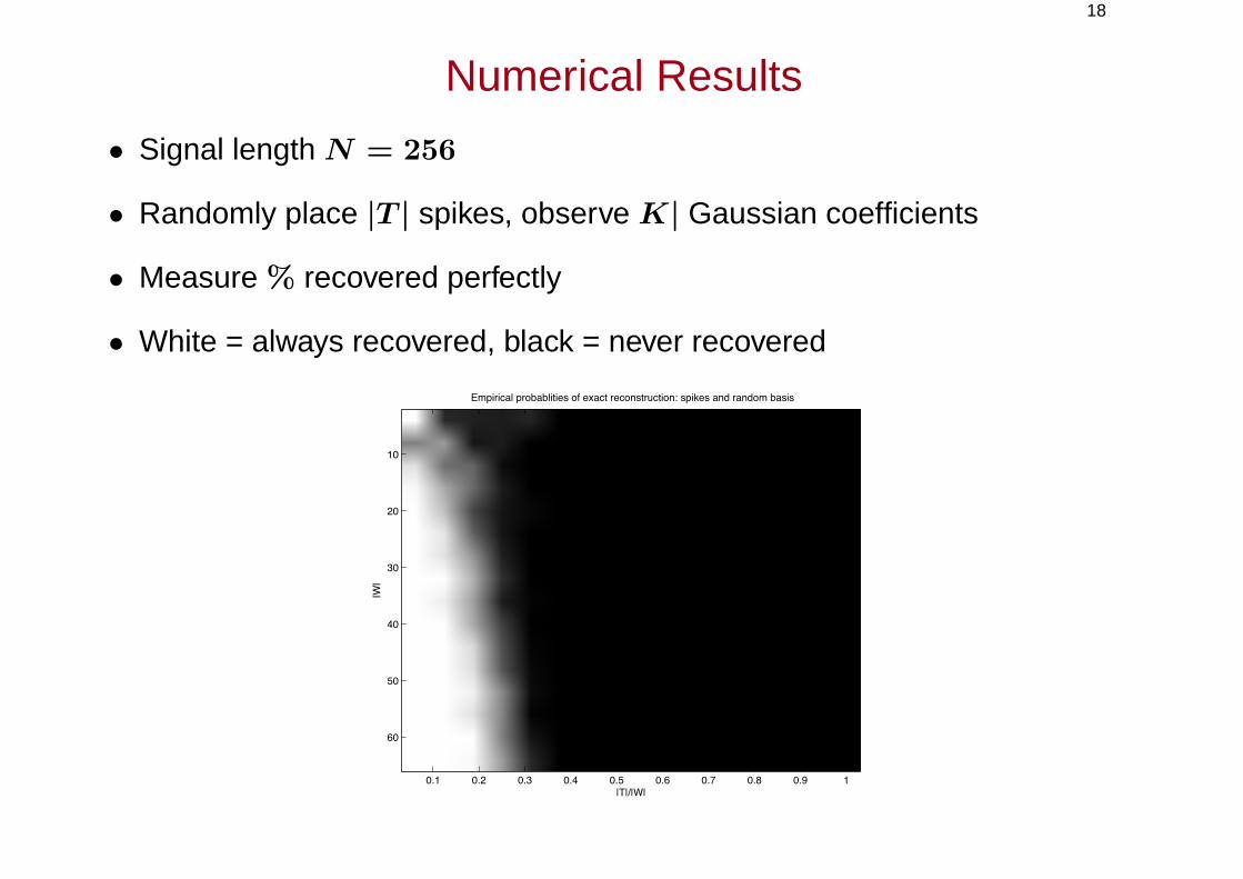
Numerical Results
• Signal length N = 256
• Randomly place |T | spikes, observe K| Gaussian coefficients
• Measure % recovered perfectly
• White = always recovered, black = never recovered
|T|/|W|
|W|
Empirical probablities of exact reconstruction: spikes and random basis
0.1 0.2 0.3 0.4 0.5 0.6 0.7 0.8 0.9 1
10
20
30
40
50
60

19
Numerical Results
• Signal length N = 1024
• Randomly place |T | spikes, observe K random frequencies
• Measure % recovered perfectly
• white = always recovered, black = never recovered
K
0.1 0.2 0.3 0.4 0.5 0.6 0.7 0.8 0.9 1
20
40
60
80
100
120
reco
very
rate
0.1 0.2 0.3 0.4 0.5 0.6 0.7 0.8 0.9 10
10
20
30
40
50
60
70
80
90
100
|T |/K |T |/K

20
Reconstruction of Piecewise Polynomials, I
• Randomly select a few jump discontinuities
• Randomly select cubic polynomial in between jumps
• Observe about 500 random coefficients
• Minimize `1 norm of wavelet coefficients
0 500 1000 1500 2000 2500−0.5
−0.4
−0.3
−0.2
−0.1
0
0.1
0.2
0.3
t
S(t
)Exact Reconstruction of a random piecewise cubic polynomial from 500 random coefficients
Original signalReconstructed signal
Reconstructed signal

21
Reconstruction of Piecewise Polynomials,II
• Randomly select 8 jump discontinuities
• Randomly select cubic polynomial in between jumps
• Observe about 200 Fourier coefficients at random
0 500 1000 1500 2000 2500−0.8
−0.6
−0.4
−0.2
0
0.2
0.4
0.6
t
S(t
)
Exact Reconstruction of a random piecewise cubic polynomial from 60 Fourier samples
Original signalReconstructed signal
Reconstructed signal

22
Reconstruction of Piecewise Polynomials, III
0 500 1000 1500 2000 2500−0.8
−0.6
−0.4
−0.2
0
0.2
0.4
0.6
t
S(t
)
Exact Reconstruction of a random piecewise cubic polynomial from 60 Fourier samples
Original signalReconstructed signal
0 500 1000 1500 2000 2500−1
−0.8
−0.6
−0.4
−0.2
0
0.2
0.4
0.6
0.8
1
t
S(t
)
Exact Reconstruction of a random piecewise cubic polynomial from 60 Fourier samples
Original signalReconstructed signal
Reconstructed signal Reconstructed signal
About 200 Fourier coefficients only!

23
Minimum TV ReconstructionMany extensions:
ming
‖g‖T V s.t. g(ω) = f(ω), ω ∈ Ω
Naive Reconstruction
50 100 150 200 250
50
100
150
200
250
Reconstruction: min BV + nonnegativity constraint
50 100 150 200 250
50
100
150
200
250
min `2 min TV – Exact!

24
Other PhantomsClassical Reconstruction
50 100 150 200 250
50
100
150
200
250
Total Variation Reconstruction
50 100 150 200 250
50
100
150
200
250
min `2 min TV – Exact!

25
Compressible Signals• In real life, signals are not sparse but most of them are compressible
• Compressible signals: rearrange the entries in decreasing order|f |2(1) ≥ |f |2(2) ≥ . . . ≥ |f |2(N)
Fp(C) = f : |f |(n) ≤ Cn−1/p, ∀n
• This is what makes transform coders work (sparse coding)
0 10 20 30 40 50 60 70 80 90 1000.1
0.2
0.3
0.4
0.5
0.6
0.7
0.8
0.9
1power decay law

26
Compressible Signals I: Wavelets in 1D
0 500 1000 1500 2000 2500−0.5
−0.4
−0.3
−0.2
−0.1
0
0.1
0.2
0.3
0.4
0.5Doppler Signal
101
102
103
104
10−16
10−14
10−12
10−10
10−8
10−6
10−4
10−2
100
102
Decay of Reordered Mother Wavelet Coefficients

27
Compressible Signals II: Wavelets in 2D
50 100 150 200 250 300 350 400 450 500
50
100
150
200
250
300
350
400
450
500
101
102
103
104
105
106
10−5
10−4
10−3
10−2
10−1
100
101
102
103
104
Decay of Reordered Mother Wavelet Coefficients
LenaBarbara

28
Compressible Signals II: Curvelets
50 100 150 200 250 300 350 400 450 500
50
100
150
200
250
300
350
400
450
500
100
101
102
103
104
105
106
10−6
10−5
10−4
10−3
10−2
10−1
100
101
102
103
Decay of Reordered Curvelet Coefficients
LenaBarbara

29
Examples of Compressible Signals
• Smooth signals. Continuous-time object has s bounded derivatives, thennth largest entry of the wavelet or Fourier coefficient sequence
|f |(n) ≤
C · n−s−1/2 1 dimension
C · n−s/d−1/2 d dimension
• Signals with bounded variations. In 2 dimensions, the BV norm of acontinuous time object is approximately
‖f‖BV ≈ ‖∇f‖L1
In the wavelet domain
|θ(f)|(n) ≤ C · n−1.
• Many other examples: e.g. Gabor atoms and certain classes of oscillatorysignals, curvelets and images with edges, etc.

30
Nonlinear Approximation of Compressible Signals
• f ∈ Fp(C), |f |(n) ≤ C · n−1/p
• Keep K-largest entries in f → fK
‖f − fK‖ ≤ C ·K−r, r = 1/p− 1/2.
• E.g. p = 1, ‖f − fK‖ ≤ C ·K−1/2.
Recovery of Compressible Signals
• How many measurements to recover f to within precision ε = K−r.
• Intuition: at least K, probably many more.

31
Where Are the Largest Coefficients?
0 5 10 15 20 25 30 35 40 45 50−1
−0.8
−0.6
−0.4
−0.2
0
0.2
0.4
0.6
0.8
1

32
Near Optimal Recovery of Compressible Signals
• Select K Gaussian random vectors (Xk), k = 1, . . . ,K
Xk ∼ N(0, IN)
• Observe yk = 〈f,Xk〉
• Reconstruct by solving (P1); minimize the `1-norm subject to constraints.
Theorem 3 (C., Tao) Suppose that f ∈ Fp(C) for 0 < p ≤ 1 or ‖f‖`1 forp = 1. Then with overwhelming probability,
‖f# − f‖2 = C · (K/ logN)−r.
See also Donoho (2004)

33
Big Surprise
Want to know an object up to an error ε; e.g. an object whose waveletcoefficients are sparse.
• Strategy 1: Oracle tells exactly (or you collect all N wavelet coefficients)which K coefficients are large and measure those
‖f − fK‖ ε
• Strategy 2: Collect K logN random coefficients and reconstruct using `1.
Surprising claim
• Same performance but with only K logN coefficients!
• Performance is achieved by solving an LP.

34
Optimality
• Can you do with fewer than K logN for accuracy K−r?
• Simple answer: NO (at least in the range K << N )

35
Optimality: Example
f ∈ B1 := f, ‖f‖`1 ≤ 1
• Entropy numbers: for a given set F ⊂ RN , we N(F , r) is the smallestnumber of Euclidean balls of radius r which cover F
ek = infr > 0 : N(F , r) ≤ 2k−1.
Interpretation in coding theory: to encode a signal from F to withinprecision ek, one would need at least k bits.
• Entropy estimates (Schutt (1984), Kuhn (2001))
ek (
log(N/k + 1)
k
)1/2
, logN ≤ k ≤ N.
To encode an object f in the `1-ball to within precision 1/√K one would
need to spend at least O(K log(N/K)) bits. For K Nβ, β < 1,O(K logN) bits.

36
Gelfand n-width (Optimality)
• k measurements Ff ; this sets the constraint that f live on an affine spacef0 + S where S is a linear subspace of co-dimension less or equal to k.
• The data available for the problem cannot distinguish any object belongingto that plane. For our problem, the data cannot distinguish between anytwo points in the intersection B1 ∩ f0 + S. Therefore, any reconstructionprocedure f∗(y) based upon y = FΩf would obey
supf∈F
‖f − f∗‖ ≥diam(B1 ∩ S)
2.
• The Gelfand numbers of a set F are defined as
ck = infS
supf∈F
‖f|S‖ : codim(S) < k,

37
Gelfand Width

38
Gelfand and entropy numbers (Optimality)
• Gelfand numbers dominate the entropy numbers (Carl, 1981)(logN/k
k
)1/2
ek / ck
• Therefore, for error 1/k
k logN/k / #meas.
• Similar argument for Fp

39
Something Special about Gaussian Measurements?
• Works with the other measurement ensembles
• Binary ensemble: F (k, t) = ±1 with prob. 1/2
‖f ] − f‖2 = C · (K/ logN)−r.
• Fourier ensemble:
‖f ] − f‖2 = C · (K/ log3N)−r.

40
Axiomatization I: Uniform Uncertainty Principle (UUP)
A measurement matrix F obeys the UUP with oversampling factor λ if for allsubsets T such that
|T | ≤ α ·K/λ,
the matrix FT obtained by extracting T columns obeys the bounds
1
2·K/N ≤ λmin(F ∗
TFT ) ≤ λmax(F ∗TFT ) ≤
3
2·K/N
This must be true w.p. at least 1 − O(N−ρ/α)

41
UUP: Interpretation
W. Heisenberg
• Suppose F is the randomly sampled DFT, Ωset of random frequencies.
• Signal f with support T obeying
|T | ≤ αK/λ
• UUP says that with overwhelming probability
‖f|Ω‖ ≤√
3K/2N‖f‖
• No concentration is possible unless K N
• “Uniform” because must hold for all such T ’s
42
Axiomatization II: Exact Reconstruction Principle(ERP)
A measurement matrix F obeys the ERP with oversampling factor λ if for eachfixed subset T
|T | ≤ α ·K/λ,
and each ‘sign’ vector σ defined on T , |σ(t)| = 1, there exists P ∈ RN s.t.
(i) P is in the row space of F
(ii) P (t) = σ(t), for all t ∈ T ;
(iii) and |P (t)| ≤ 12
for all t ∈ T c
Interpretation: Gives exact reconstruction for sparse signals

43
Near-optimal Recovery Theorem [C., Tao]
• Measurement ensemble obeys UUP with oversampling factor λ1
• Measurement ensemble obeys ERP with oversampling factor λ2
• Object f ∈ Fp(C).
‖f − f ]‖ ≤ C · (K/λ)−r, λ = max(λ1, λ2).

44
UUP for the Gaussian Ensemble
• F (k, t) = Xk,t/√N
• Singular values of random Gaussian matrices
(1 −√c) ·
√K
N/ σmin(FT ) ≤ σmax(FT ) / (1 +
√c) ·
√K
N
with overwhelming probability (exceeding 1 − e−βK).
Reference, S. J. Szarek, Condition numbers of random matrices, J.Complexity (1991),
See also Ledoux (2001), Johnstone (2002), El-Karoui (2004)
• Marchenko-Pastur law: c = |T |/K.
• Union bound give result for all T provided
|T | ≤ γ ·K/(logN/K).

45
ERP for the Gaussian Ensemble
P = F ∗FT (F ∗TFT )−1sgn(f) := F ∗V.
• P is in the row space of F
• P agrees with sgn(f) on T
P|T = F ∗TFT (F ∗
TFT )−1sgn(f) = sgn(f)
• On the complement of T : P|T c = F ∗T cV .
P (t)1
√N
K∑k=1
Xk,tVk.
• By independence of F ∗T c and V , conditional distribution
L(P (t)|V ) ∼ N(0, ‖V ‖2/N)

46
• With overwhelming probability (UUP)
‖V ‖ ≤ ‖FT (F ∗TFT )−1‖ · ‖sgn(f)‖ ≤
√6N/K ·
√|T |
so that
L(P (t)|V ) ∼ N(0, σ2). σ2 ≤ 6|T |/K
• In conlusion: for t ∈ T c
P (P (t) > 1/2) ≤ e−βK/|T |.
• ERP holds if
|K| ≥ α · |T | · logN.

47
Universal Codes
Want to compress sparse signals
• Encoder. To encode a discrete signal f , the encoder simply calculates thecoefficients yk = 〈f,Xk〉 and quantizes the vector y.
• Decoder. The decoder then receives the quantized values andreconstructs a signal by solving the linear program (P1).
Conjecture Asymptotically nearly achieves the information theoretic limit.

48
Information Theoretic Limit: Example
• Want to encode the unit-`1 ball: f ∈ RN :∑
t |f(t)| ≤ 1.
• Want to achieve distortion D
‖f − f ]‖2 ≤ D
• How many bits? Lower bounded by entropy of the unit-`1 ball:
# bits ≥ C ·D · (log(N/D) + 1)
• Same as number of measured coefficients

49
Robustness
• Say with K coefficients
‖f − f ]‖2 1/K
• Say we loose half of the bits (packet loss). How bad is the reconstruction?
‖f − f ]50%‖2 2/K
• Democratic!

50
Reconstruction from 100 Random Coefficients
0 200 400 600 800 1000 1200−2
−1
0
1
2
3
4
5
6Reconstruction of "Blocks" from 100 random coefficients
Original signalReconstructed signal
’Compressed’ signal

51
Reconstruction from Random Coefficients
0 200 400 600 800 1000 1200−0.6
−0.5
−0.4
−0.3
−0.2
−0.1
0
0.1
0.2Reconstruction of "CUSP" from 150 random coefficients
Original signalReconstructed signal
0 200 400 600 800 1000 1200−0.8
−0.6
−0.4
−0.2
0
0.2
0.4
0.6Reconstruction of "Doppler" from 200 random coefficients
Original signalReconstructed signal
Cusp from 150 coeffs. Doppler from 200 coeffs.

52
Reconstruction from Random Coefficients (Method II)
0 200 400 600 800 1000 1200−0.6
−0.5
−0.4
−0.3
−0.2
−0.1
0
0.1
0.2Reconstruction of "Cusp" from 150 random coefficients
Original signalReconstructed signal

53
Summary
• Possible to reconstruct a compressible signal from a few measurementsonly
• Need to randomize measurements
• Need to solve an LP
• This strategy is nearly optimal
• Many applications