Embed Size (px)
Citation preview

Near isotropic behavior of turbulent thermal convection Nath, D, Pandey, A, Kumar, A & Verma, MK
Author post-print (accepted) deposited by Coventry University’s Repository Original citation & hyperlink:
Nath, D, Pandey, A, Kumar, A & Verma, MK 2016, 'Near isotropic behavior of turbulent thermal convection' Phys. Rev. Fluids, vol 1, pp. 064302. https://dx.doi.org/10.1103/PhysRevFluids.1.064302
DOI 10.1103/PhysRevFluids.1.064302 ESSN 2469-990X Publisher: American Physical Society Copyright © and Moral Rights are retained by the author(s) and/ or other copyright owners. A copy can be downloaded for personal non-commercial research or study, without prior permission or charge. This item cannot be reproduced or quoted extensively from without first obtaining permission in writing from the copyright holder(s). The content must not be changed in any way or sold commercially in any format or medium without the formal permission of the copyright holders. This document is the author’s post-print version, incorporating any revisions agreed during the peer-review process. Some differences between the published version and this version may remain and you are advised to consult the published version if you wish to cite from it.

Near isotropic behavior of turbulent thermal convection
Dinesh Nath,∗ Ambrish Pandey,† Abhishek Kumar,‡ and Mahendra K. Verma§
Department of Physics, Indian Institute of Technology Kanpur, Kanpur 208016, India
We investigate the anisotropy in turbulent convection in a 3D box using direct numerical
simulation. We compute the anisotropic parameter A = u2⊥/(2u2‖), where u⊥ and u‖ are the
components of velocity perpendicular and parallel to the buoyancy direction, the shell and
ring spectra, and shell-to-shell energy transfers. We observe that the flow is nearly isotropic
for the Prandtl number Pr ≈ 1, but the anisotropy increases with the Prandtl number. For
Pr = ∞, A ≈ 0.3, thus anisotropy is not very significant even in extreme cases. We also
observe that u‖ feeds energy to u⊥ via pressure. The computation of shell-to-shell energy
transfers reveals that the energy transfer in turbulent convection is local and forward, similar
to hydrodynamic turbulence. These results are consistent with the Kolmogorov’s spectrum
observed by Kumar et al. [Phys. Rev. E 90, 023016 (2014)] for turbulent convection.
PACS numbers: 47.27.E-,47.27.te,47.27.ek
∗ [email protected]† [email protected]‡ [email protected]§ [email protected]

2
I. INTRODUCTION
Kolmogorov’s theory of turbulence [1–3] describes the flow properties of hydrodynamic turbu-
lence under the assumption of homogeneity and isotropy of the flow. This approximation is valid
for idealized flows having no external fields or confining walls. Most practical flows however involve
external fields and walls, hence they could have significant anisotropy, and their behaviour could
differ from Kolmogorov’s theory. Some of the examples of anisotropic turbulent flows are magneto-
hydrodynamic (MHD) turbulence [4], rotating turbulence ([5] and references their in), quasi-static
liquid-metal flows [6–9], turbulent convection [10], and rotating convection [11]. In this paper we
will study anisotropy in turbulent convection.
Group theory is used to characterize properties of system obeying certain symmetries. Lohse
and Muller-Groeling [12], Kurien and Sreenivasan [13], and Biferale and Procaccia [14] expanded
the velocity correlation function of isotropic hydrodynamic turbulence using spherical harmonics;
under this expansion, the correlation function is spherically symmetric only to the lowest order.
Experiments and numerical simulations (see review [14] for references) reveal presence of higher-
order terms of SO(3) decomposition in the velocity correlation function, thus they demonstrate
deviations from the spherical symmetry, a signature of anisotropy. However, the external gravi-
tational field of the RBC breaks the isotropy of the system and the equation. Thus, the degree
of anisotropy in RBC is expected to be larger than that in isotropic hydrodynamic turbulence.
Biferale et al. [15] studied anisotropy in the small-scale turbulence of convection and random Kol-
mogorov flow using structure function. They showed that the anisotropic scaling properties of
these two systems are reasonaly similar.
Rayleigh-Benard convection (RBC) is a popular model for studying convective flows [16–18].
RBC is quantified using two parameters: Rayleigh number Ra, which is a measure of the ratio
of buoyancy and dissipative force, and Prandtl number Pr, which is the ratio of the kinematic
viscosity and thermal diffusivity. The flow becomes turbulent at large Ra, but it is viscous at very
large Pr. In this paper we study anisotropy in RBC for a wide range of Pr, from very small value
to infinity.
Researchers have attempted to quantify anisotropy in turbulent flow using several parameters.
Shebalin et al. [4] proposed a measure for a quantity Q in two-dimensional magnetohydrodynamic
turbulence. Some authors (e.g., Sagaut and Cambon [5] and references therein) used Craya decom-
position to quantify toroidal and poloidal components of a vector field. Teaca et al. [19] decomposed
the Fourier space into rings and studied energy contents in them, which provides information about

3
the angular dependence of the energy. They also studied energy exchanges among such rings. For
quasi-static MHD, Favier et al. [6–8] analyzed anisotropy by studying the ratio of the energies of
the transverse and parallel components; they quantified the finer details of anisotropy in terms of
polar angles using the toroidal and poloidal decomposition [5]. Delache et al. [20] performed similar
analysis for rotating turbulence. Reddy and Verma [9] and Reddy et al. [21] studied quasi-static
MHD using wavenumber rings, and showed how energy is transferred from the parallel component
of velocity to the perpendicular component of velocity via pressure.
Anisotropy in RBC has not been studied in detail. In one of the works, Rincon [10] derived
the SO(3) decomposition of structure functions analytically and then computed them numerically.
He showed that the third-order structure function 〈(∆θ)2∆u〉 appearing in the Yaglom equation
exhibits a clear scaling exponent of unity for a small range of scales. He argued that buoyancy can
deviate the energy spectrum from the Kolmogorov’s 5/3 power law. Kunnen et al. [11] showed that
rotation enhances anisotropy in turbulent convection, with centre plane being rod-like, while the
region near the top plates being nearly isotropic. Biferale et al. [15] quantified anisotropy in the
small-scale turbulence of RBC by decomposing the structure function using spherical harmonics.
Another class of buoyancy-driven flows is Rayleigh-Taylor instability (RTI) [22, 23] that has a
very similar instability mechanism as RBC (heavy fluid on top of lighter fluid). Cabot and Zhou [24]
and other researchers studied anisotropy for RTI. Unstably stratified homogeneous turbulence
(USHT) is a class of RTI in which the integral length of turbulence is much smaller compared to
the mixing zone width. Soulard et al. [25] and Burlot et al. [26] studied the phenomenology, spectral
modelling, and anisotropy of USHT. In the Conclusions and Discussions section, we contrast the
observed anisotropy of RBC and USHT.
In this paper, we perform direct numerical simulation (DNS) of turbulent and laminar RBC
flows in a box for different values of Pr and Ra and quantify anisotropy in turbulent convection
using several measures. We use anisotropy parameter A = u2⊥/(2u2‖), where u⊥ and u‖ are the
components of velocity perpendicular and parallel to the buoyancy direction respectively. Next we
use ring spectrum to differentiate the energy contents at different polar angles in the Fourier space.
Our simulations reveal nearly isotropic flows, specially for Pr ≈ 1. After this we compute the
energy flux and shell-to-shell energy transfers, and show them to be quite close to those observed
in hydrodynamic turbulence. Energetically u‖ is accelerated by buoyancy. We show using energy
transfer computation that u‖ feeds energy to u⊥ via pressure.
The outline of the paper is as follows: In Sec. II, we discuss the equations governing the dynamics
of Rayleigh-Bendard convection. In Sections III and IV, we describe respectively the frameworks

4
of anisotropic energy distribution and anisotropic energy transfers used in this paper. We detail
the numerical simulations in Sec. V, and numerical results of energy spectra and energy transfers
in Secs. VI and VII respectively. Finally, we conclude in Sec. VIII.
II. GOVERNING EQUATIONS
The dynamical equations that describe RBC under Boussinesq approximation are [27]
∂u
∂t+ (u · ∇)u = − 1
ρ0∇σ + αgθz + ν∇2u, (1)
∂θ
∂t+ (u · ∇)θ =
∆
duz + κ∇2θ, (2)
∇ · u = 0, (3)
where u is the velocity field, θ and σ are the temperature and pressure fluctuations from the
conduction state respectively, and z is the buoyancy direction. Here α is the thermal expansion
coefficient, g is the acceleration due to gravity, and ρ0, ν, κ are the fluid’s mean density, kinematic
viscosity and thermal diffusivity respectively. We consider fluid between two horizontal plates that
are separated by a distance d. The temperature difference between the two plates is ∆.
We nondimensionalize Eqs. (1-3) using d as the length scale, (αg∆d)1/2 as the velocity scale,
and ∆ as the temperature scale, which yields,
∂u
∂t+ (u · ∇)u = −∇σ + θz +
√Pr
Ra∇2u, (4)
∂θ
∂t+ (u · ∇)θ = uz +
1√RaPr
∇2θ, (5)
∇ · u = 0. (6)
The two nondimensional parameters are the Prandtl number
Pr =ν
κ, (7)
and the Rayleigh number
Ra =αg∆d3
νκ. (8)
We solve the aforementioned equations using pseudospectral method in Fourier space. In our
simulations, for the velocity field, we employ the free-slip boundary condition at all the walls.
However, for the temperature field, we employ conducting boundary condition at the top and
bottom plates, but insulating boundary condition at the side walls.

5
The buoyancy accelerates a fluid parcel along z, hence it is expected to induce anisotropy in
the flow. Surprisingly, the induced anisotropy is not very significant. In the next two sections we
will describe tools to characterize the anisotropy in RBC.
III. QUANTIFICATION OF ANISOTROPIC DISTRIBUTION OF ENERGY IN RBC
In this section, we discuss the anisotropy measures in RBC. One such measure is the anisotropy
parameter A defined as [9]
A =E⊥2E‖
=u2⊥2u2‖
=〈u2x + u2y〉
2〈u2z〉. (9)
Here 〈.〉 represents averaged quantity per unit volume. For an isotropic flow, 〈u2x〉 = 〈u2y〉 = 〈u2z〉,
hence A = 1. In RBC, 〈u2x〉 = 〈u2y〉 < 〈u2z〉 because buoyancy preferentially accelerates the flow
along z. Therefore, A < 1 for RBC.
We quantify the energy at different length scales using the shell spectrum, which is defined as
E(k) =∑
k−1<k′≤k
1
2|u(k′)|2 (10)
is the sum of the energy of all the Fourier modes [u(k′)] in a given shell of radius k and unit width.
Thus E(k) masks the anisotropic features of the flows. For anisotropic flows, we divide a shell
into rings as shown in Fig. 1. Here each shell is divided into rings that are characterized by two
indices—the shell index k, and the sector index β [9, 19]. We name the rings containing ζ = 0 and
ζ = π/2 as the polar and the equatorial rings respectively. The gravitational field is aligned along
ζ = 0. The energy spectrum of a ring, called the ring spectrum, is defined as
E (k, β) =1
Cβ
∑k−1<k′≤k;
∠(k′)∈(ζβ−1,ζβ]
1
2
∣∣u (k′)∣∣2 , (11)
where ∠k′ is the angle between k′ and the unit vector z. The sector β contains the modes between
the angles ζβ−1 to ζβ is shown in Fig. 1(b). For a uniform ∆ζ, sectors near the equator contain
more modes than those near the poles. To compensate the above, we divide the sum∑
k |u(k′)|2/2
by the factor C(β) given by
Cβ = |cos (ζβ−1)− cos (ζβ)| . (12)
We obtain further insights into the physics of convection by computing the ring spectra of the

6
FIG. 1. (a) Schematic diagram of ring decomposition in Fourier space. (b) Schematic diagram of a vertical
section of the Fourier space exhibiting wavenumber rings, sectors, and shells.
perpendicular and parallel components of the velocity:
E⊥(k, β) =1
Cβ
∑k−1<k′≤k;
∠(k′)∈(ζβ−1,ζβ]
1
2
∣∣u⊥ (k′)∣∣2 (13)
E‖(k, β) =1
Cβ
∑k−1<k′≤k;
∠(k′)∈(ζβ−1,ζβ]
1
2
∣∣u‖ (k′)∣∣2 (14)
where u‖ = u · z and u⊥ = u − u‖z. Clearly, the ring spectrum for the total energy E(k, β) =
E⊥(k, β) + E‖(k, β). We can also define energy contents of a sector β as
E(β) =∑k
E(k, β); E⊥,‖(β) =∑k
E⊥,‖(k, β). (15)
We will compute the above spectra for RBC with various Prandtl and Rayleigh numbers. We also
quantify the anisotropy using Legendre polynomials. For the same, we expand the ring spectrum
of the total energy using Legendre polynomials.
Earlier Shebalin et al. [4] quantified anisotropy for a quantity Q in two-dimensional magneto-
hydrodynamic turbulence using angle θQ that is defined as
θQ = tan−1∑
k k2zQ(k)∑
k k2xQ(k)
. (16)
In three dimensions, the above formula generalizes to
θQ = tan−1∑
k 2k2zQ(k)∑k(k2x + k2y)Q(k)
. (17)

7
The ring spectrum proposed in this paper provides more detailed information than the angular
measure of Shebalin et al. [4].
IV. FORMALISM OF ENERGY TRANSFERS IN RBC
The nonlinearity in fluid flows induces energy transfers among Fourier modes. In three-
dimensional hydrodynamic turbulence, it is known that the energy transfers are forward (from
low-wavenumber shells to higher-wavenumber shells) and local (maximal transfer to the neighbour-
ing shell). In this paper we will investigate whether turbulent convection has a similar behaviour.
We also propose several formulae that capture anisotropic energy transfers in RBC. In the first two
subsections, we discuss the energy flux and shell-to-shell energy transfers that describe the isotropic
energy exchanges. In the next two subsections, we describe the ring-to-ring energy transfers and
energy exchange between the parallel and perpendicular components of the velocity field.
A. Energy flux
Using Eqs. (1,2) we derive the equation for the kinetic energy in RBC, which is
∂E (k)
∂t= T (k) + F (k)−D (k) , (18)
where T (k) is the energy transfer rate to the shell k due to nonlinear interactions, F (k) is the
energy supply rate to the shell due to buoyancy, and D (k) is the viscous dissipation rate, which
are defined as
F (k) =∑|k′|=k
<〈uz(k′)θ∗(k′)〉, (19)
D (k) =∑|k′|=k
2
√Pr
Rak′2E
(k′), (20)
where < and ∗ represent the real part and the complex conjugate of a complex number respectively.
The nonlinear interaction term T (k) leads to energy transfers among modes leading to a kinetic
energy flux Π (k0), which is defined as
Π(k0) = −∫ k0
0T (k)dk.
Physically, Π(k0) represents the net energy transfers from the modes inside the wavenumber sphere
of radius k0 to modes outside the sphere [28].

8
The energy flux Π(k0) is computed using the Fourier space data by employing the mode-to-mode
energy transfer [29, 30]. In this framework, we can compute the energy transfers among Fourier
modes within an interacting wavenumber triad k,p,q. Note that these wavenumbers satisfy a
relation k = p + q. Here, the rate of energy transfer from the velocity mode u(p) to the velocity
mode u(k) with the velocity mode u(q) acting as a mediator is
S (k |p|q) = ={[k · u (q)] [u∗ (k) · u (p)]} , (21)
where = represents the imaginary part of a complex number. In terms of the above formula, the
energy flux is
Π(k0) =∑k>k0
∑p≤k0
S (k |p|q) . (22)
The energy flux provides energy emanating from a wavenumber sphere. A more detailed picture
of the energy transfers is provided by the shell-to-shell energy energy transfers that will be discussed
in the next subsection.
B. Shell-to-shell energy transfers
We divide the wavenumber space into a set of wavenumber shells. The shell-to-shell energy
transfer rate from the velocity field of the mth shell to the velocity field of the nth shell is defined
as [29, 30]
Tmn =∑k∈n
∑p∈m
S (k |p|q) . (23)
In Kolmogorov’s theory of hydrodynamic turbulence, the maximum shell-to-shell energy transfer
occurs from shell m to shell (m+ 1), hence the energy transfer in hydrodynamic turbulence is local
and forward. We will explore using numerical simulations whether the energy transfer in RBC is
local and forward.
Unfortunately both the aforementioned measures of energy transfers do not capture the
anisotropic effects since the energy flux and shell-to-shell energy transfers provide averaged values
over the polar angle ζ. In the next two subsections we quantify anisotropic energy transfers using
ring-to-ring energy transfers and the energy exchange between the perpendicular and parallel
components of the velocity field.
9
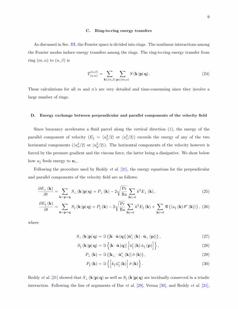
C. Ring-to-ring energy transfers
As discussed in Sec. III, the Fourier space is divided into rings. The nonlinear interactions among
the Fourier modes induce energy transfers among the rings. The ring-to-ring energy transfer from
ring (m,α) to (n, β) is
T(n,β)(n,α) =
∑k∈(n,β)
∑p∈(m,α)
S (k |p|q) . (24)
These calculations for all m and n’s are very detailed and time-consuming since they involve a
large number of rings.
D. Energy exchange between perpendicular and parallel components of the velocity field
Since buoyancy accelerates a fluid parcel along the vertical direction (z), the energy of the
parallel component of velocity (E‖ = 〈u2‖/2〉 or 〈u2z/2〉) exceeds the energy of any of the two
horizontal components (〈u2x/2〉 or 〈u2y/2〉). The horizontal components of the velocity however is
forced by the pressure gradient and the viscous force, the latter being a dissipative. We show below
how u‖ feeds energy to u⊥.
Following the procedure used by Reddy et al. [21], the energy equations for the perpendicular
and parallel components of the velocity field are as follows:
∂E⊥ (k)
∂t=
∑k=p+q
S⊥ (k |p|q) + P⊥ (k)− 2
√Pr
Ra
∑|k|=k
k2E⊥ (k) , (25)
∂E‖ (k)
∂t=
∑k=p+q
S‖ (k |p|q) + P‖ (k)− 2
√Pr
Ra
∑|k|=k
k2E‖ (k) +∑|k|=k
<(〈u‖ (k) θ∗ (k)〉
), (26)
where
S⊥ (k |p|q) = ={[k · u (q)] [u∗⊥ (k) · u⊥ (p)]} , (27)
S‖ (k |p|q) = ={
[k · u (q)][u∗‖ (k) u‖ (p)
]}, (28)
P⊥ (k) = ={[k⊥ · u∗⊥ (k)] σ (k)} , (29)
P‖ (k) = ={[k‖u∗‖ (k)
]σ (k)
}. (30)
Reddy et al. [21] showed that S⊥ (k |p|q) as well as S‖ (k |p|q) are invidually conserved in a triadic
interaction. Following the line of arguments of Dar et al. [29], Verma [30], and Reddy et al. [21],

10
we can define energy fluxes of the perpendicular and parallel components of the velocity field as
Π⊥(k′)
=∑|k|≥k′
∑|p|<k′
S⊥ (k |p|q) (31)
Π‖(k′)
=∑|k|≥k′
∑|p|<k′
S‖ (k |p|q) . (32)
It is important to note that there is no direct energy transfer from the parallel component to the
perpendicular component, i.e., the nonlinear transfer does not have terms of the type [u∗⊥ (k)·u‖ (p)]
(which would anyway vanish since they are perpendicular to each other).
The energy equations [Eqs. (25,26)] reveal that E⊥ receives energy from E‖ by an amount
P⊥ (k). Interestingly, the incompressibility condition [k · u (k) = 0] yields
P⊥ (k) = −P‖ (k) . (33)
That is, the energy gained by the perpendicular component u∗⊥ (k) via pressure is equal and opposite
to the energy lost by the parallel counterpart. The pressure aids the energy exchange between the
perpendicular and parallel components of velocity field. The total flux Π is the sum of Π⊥ and Π‖.
We will study the above transfers for RBC in Sec. VII using numerical data. In the next section
we will describe simulation details.
V. SIMULATION DETAILS
We perform direct numerical simulation of RBC in a cube of unit size (aspect ratio one) using
a pseudo-spectral solver Tarang [31]. We employ a 5123 grid for our simulations. The nondimen-
sional equations [Eqs. (4–6)] are evolved in time by the fourth order Runge-Kutta method. The
CFL (Courant-Friedrichs-Lewy) condition is used for calculating the time step ∆t (a typical value
is 0.01), and the 3/2 rule for the dealiasing.
The boundary conditions employed in this work are as follows: free-slip boundary condition
for the velocity at all the walls, conducting boundary condition for the temperature at the top
and bottom walls, and insulating boundary condition for the temperature at the vertical walls. We
remark that the energy spectra and energy transfer studies are best performed in the Fourier space.
The free-slip boundary condition facilitates transformation to the Fourier space quite naturally, in
contrast to the no-slip boundary condition for which one needs to invoke Chebyshev polynomials.
This is one of the reasons for choosing the free-slip boundary condition for our simulation. Note
that the energy spectrum and energy transfers in the bulk of the flow are expected to be similar for
the free-slip and no-slip boundary conditions. In Fig. 2, we show the (horizontal) planar-averaged

11
TABLE I. RBC simulation parameters with grid resolution of 5123: Prandtl number Pr, Rayleigh number
Ra, Reynolds number Re, kmaxη, E⊥/2, E‖, anisotropic parameter A = E⊥/(2E‖), integral length scale l,
vertical integral length scale lz, and the total viscous dissipation rate D.
Pr Ra Re kmaxη 0.5E⊥ E‖ A l lz D
0.02 2× 10⁶ 7.05× 10³ 3.4 0.118 0.187 0.63 0.478 0.553 1.02× 10⁻⁴
1 108 3.11× 10³ 5.9 0.013 0.018 0.73 0.468 0.547 1.02× 10⁻⁴
6.8 108 9.08× 10² 3.2 0.010 0.017 0.59 0.484 0.591 2.65× 10⁻⁴
100 108 1.25× 10² 1.6 0.002 0.004 0.49 0.531 0.635 1.02× 10⁻³
∞ 2× 10⁸ 0 4.2 0.221 0.725 0.30 0.449 0.716 7.21× 10⁻⁵
0.0 0.2 0.4 0.6 0.8 1.0T(z)
0.0
0.2
0.4
0.6
0.8
1.0
z
Pr =0.02
Pr =1
Pr =6.8
Pr =100
Pr =∞
FIG. 2. Plot of the instantaneous temperature profile T (z) =∫dxdyT (x, y, z) vs. z. that exhibits
T (z) ≈ 1/2 in the bulk, and sharp variations near the walls.
temperature T (z) as a function of z, where T (z) =∫dxdyT (x, y, z). The figure shows that T (z)
has a sharp gradient near the walls, and an approximate constant value (≈ 1/2) in the bulk.
We initiate an RBC simulation on a smaller grid and continue it until the steady state is reached.
The final state of this simulation is used as an initial condition for a simulation on a larger grid for
a set of larger parameters (Pr and Ra). The final run is performed on 5123 grid size. The various
values of Pr and Ra considered in this work are listed in Table I. In each simulation, the quantity
kmaxη remains greater than unity implying that the simulations are well resolved. Here kmax is
the maximum wavenumber, and η represents the Batchelor length (ηθ), except for Pr = 0.02,
for which η represent the Kolmogorov length (ηu). Since the box size d = 1, the wavenumber
k = π(nx, ny, nz), where nx, ny, nz are integers. Therefore, ∆kx = ∆ky = ∆kz = π, the smallest

12
wavevectors in system are k = π(x+ z) and k = π(y + z), and hence kmin = π√
2.
We compute the integral length l, and vertical integral length lz using the formulae:
l =
∑k E(k)(π/k)∑
k E(k)(34)
lz =
∑k
∑β E(k, β)(π/kz)∑k
∑β E(k, β)
(35)
where kz = k cos ζ with ζ as the mean angle in the sector β. The computed values of l and lz, listed
in Table I, are comparable to the box size. Note that lz > l with the maximum lz occurring for
Pr = ∞, and minimum for Pr = 1, which is connected to the elongation of the plumes for larger
Pr. Thus, the least anisotropic flow occurs for Pr = 1, and most anisotropic one for Pr =∞. This
feature will be discussed in the following sections.
VI. NUMERICAL RESULTS ON ENERGY DISTRIBUTION IN RBC
In this section we describe the energy distribution in turbulent RBC for various Prandtl num-
bers. In Fig. 3 we exhibit the time series of the steady-state values of E⊥/(2E), E‖/E, and the
anisotropy parameter A = E⊥/(2E‖) for Pr = 0.02, 1, 6.8, 100, and ∞. The average values of A for
these parameters are 0.63, 0.73, 0.59, 0.49 and 0.30 respectively (listed in Table I), consistent with
the argument that buoyancy yields u2‖ > (u2⊥/2). These results demonstrate that the flow is least
anisotropic (maximum A) for Pr = 1, and most anisotropic (minimum A) for Pr = ∞, consistent
with our computations of integral length scales. Note however that in the extreme case, Pr =∞,
Ey and Ex are approximately 30% of Ez. Hence, the flow is not far from isotropy even for extreme
cases (large and infinite Prandtl numbers). Table I also lists the total viscous dissipation rate,
which is quite small for all our runs.
Next, we compute the energy spectra E(k), E⊥(k), and E‖(k) for Pr = 0.02, 1, 6.8,∞. We
observe that E‖(k) > E⊥(k)/2 for all the cases, with the divergence between E‖(k) and E⊥(k)/2
being maximum for Pr = ∞ (see Fig. 4). For a small inertial range, we observe E(k) ∼ k−5/3 for
Pr = 0.02, 1, 6.8, and E(k) ∼ k−13/3 for Pr = ∞, consistent with the earlier results of Kumar et
al. [32] and Pandey et al. [33] respectively. The power-law regime is rather small due to relatively
smaller grid resolutions in our simulations.
To explore whether the flow is homogeneous and isotropic, we take various horizontal and
vertical sections of the flow at y = 0.10, 0.25, 0.5, 0.75, 0.90 and z = 0.10, 0.25, 0.5, 0.75, 0.90. We
compute the normalized two-dimensional energy spectra for these sections for k in the inertial

13
0.1
0.5
0.9
(a) 0.5E⊥/E E‖/E A
0.1
0.5
0.9(b)
0.1
0.5
0.9
Ratios o
f energ
ies
(c)
0.1
0.5
0.9(d)
20 30 40 50 60 700.1
0.5
0.9
t
(e)
FIG. 3. Time series of E⊥/(2E), E‖/E, and A = E⊥/(2E‖) for (a) Pr = 0.02, Ra = 2× 10⁶, (b) Pr = 1,
Ra = 108, (c) Pr = 6.8, Ra = 108, (d) Pr = 100, Ra = 108, and (e) Pr =∞, Ra = 2× 10⁸.
range. In Fig. 5(a,b) we present these spectra for Pr = 1,Ra = 108. The plots nearly overlap with
each other, thus demonstrating near homogeneity and isotropy of the flow.
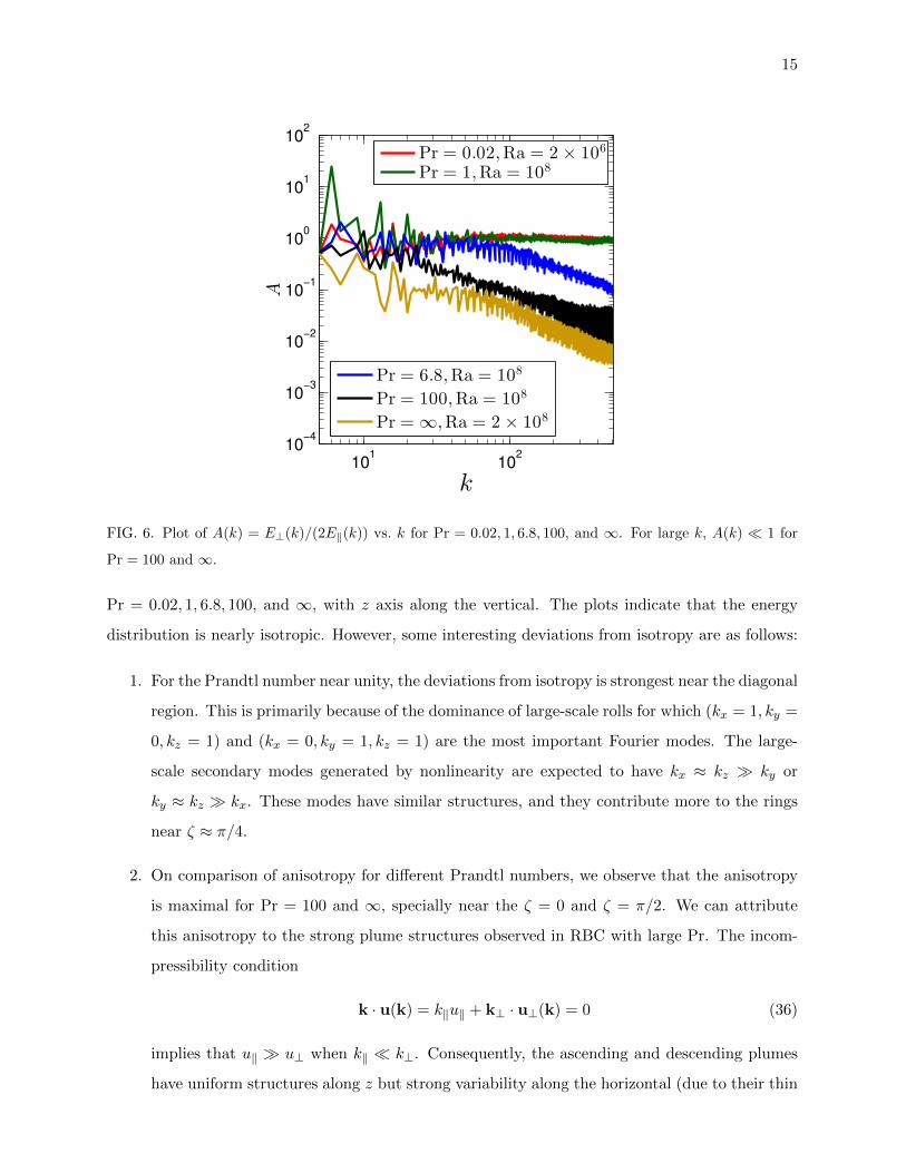
In Fig. 6 we plot the anisotropic parameter A(k) = E⊥(k)/(2E‖(k)) vs. k that quantifies the
scale-by-scale anisotropy. We observe that for large k, A(k) ≈ 1 for Pr = 0.02, 1. For large and
infinite Pr, A(k) � 1 with A(k) decreasing with k after k > 50 or so. Thus, the flows with large
and infinite Pr are strongly anisotropic at small scales (k � 1), a feature related to the thin plumes.
We will revisit this aspect while discussing the ring spectrum.
Now we compute the ring spectra E(k, β), defined in Sec. III, for various Prandtl numbers. For
this we have divided the Fourier space into shells of unit radius from k = 0 to kmax = πN (grid
size = N3), and 20 sectors with ∆ζ of 4.5 degrees each. In Fig. 7 we exhibit the ring spectra for

14
Norm
aliz
ed K
E
100
10−2
10−4
10−6
(a)
E (k)k5/3
0.5E⊥ (k)k5/3
E‖ (k)k5/3
100
10−2
10−4
10−6
(b)
E (k)k5/3
0.5E⊥ (k)k5/3
E‖ (k)k5/3
101
102
k
Norm
aliz
ed K
E
100
10−2
10−4
10−6
10−8
(c)
E (k)k5/3
0.5E⊥ (k)k5/3
E‖ (k)k5/3
101
102
k
10−4
10−2
100
102
104 (d)
E (k)k13/3
0.5E⊥ (k)k13/3
E‖ (k)k13/3
FIG. 4. Plots of normalized kinetic energy spectrum E(k)kα vs. k for (a) Pr = 0.02, Ra = 2 × 10⁶, (b)
Pr = 1, Ra = 108, (c) Pr = 6.8, Ra = 108, and (d) Pr = ∞, Ra = 2 × 10⁸. Black dashed lines depict the
power-law regimes.
101 102 103
k
10-7
10-5
10-3
10-1
101
Exz
u(k
)k5/
3
(a)
y=0.10
y=0.25
y=0.50
y=0.75
y=0.90
101 102 103
k
10-7
10-5
10-3
10-1
101
Exy
u(k
)k5/
3
(b)
z=0.10
z=0.25
z=0.50
z=0.75
z=0.90
FIG. 5. For Pr = 1,Ra = 108, plots of two-dimensional normalized kinetic spectra: (a) Exzu (k)k5/3 for
vertical sections at y = 0.10, 0.25, 0.5, 0.75, 0.90, and (b) Exyu (k)k5/3 for the horizontal sections at z =
0.10, 0.25, 0.5, 0.75, 0.90. The near overlapping plots demonstrate near homogeneity and isotropy of the
flow.
15
101
102
10−4
10−3
10−2
10−1
100
101
102
k
A
Pr = 0.02,Ra = 2 × 10⁶
Pr = 1,Ra = 108
Pr = 6.8,Ra = 108
Pr = 100,Ra = 108
Pr = ∞,Ra = 2 × 10⁸
FIG. 6. Plot of A(k) = E⊥(k)/(2E‖(k)) vs. k for Pr = 0.02, 1, 6.8, 100, and ∞. For large k, A(k) � 1 for
Pr = 100 and ∞.
Pr = 0.02, 1, 6.8, 100, and ∞, with z axis along the vertical. The plots indicate that the energy
distribution is nearly isotropic. However, some interesting deviations from isotropy are as follows:
1. For the Prandtl number near unity, the deviations from isotropy is strongest near the diagonal
region. This is primarily because of the dominance of large-scale rolls for which (kx = 1, ky =
0, kz = 1) and (kx = 0, ky = 1, kz = 1) are the most important Fourier modes. The large-
scale secondary modes generated by nonlinearity are expected to have kx ≈ kz � ky or
ky ≈ kz � kx. These modes have similar structures, and they contribute more to the rings
near ζ ≈ π/4.
2. On comparison of anisotropy for different Prandtl numbers, we observe that the anisotropy
is maximal for Pr = 100 and ∞, specially near the ζ = 0 and ζ = π/2. We can attribute
this anisotropy to the strong plume structures observed in RBC with large Pr. The incom-
pressibility condition
k · u(k) = k‖u‖ + k⊥ · u⊥(k) = 0 (36)
implies that u‖ � u⊥ when k‖ � k⊥. Consequently, the ascending and descending plumes
have uniform structures along z but strong variability along the horizontal (due to their thin

16
structures). The other regime k⊥ � k‖ has u⊥ � u‖ that corresponds to the horizontal
flow near the top and bottom plates. Thus, the incompressibility plays a major role in the
determination of anisotropic structures in RBC.
To highlight the angular dependence of the ring spectrum, in Fig. 8 we plot the energy in the
sector β, E(β), E⊥(β), and E‖(β) as a function of ζ [refer to Eq. (15)]. The plots indicate a peak
in these spectra near ζ = π/4, consistent with the fact that the maximum of the energy spectrum
occurs near the diagonal region. We also observe strong E⊥(k, β) and E‖(k, β) for ζ ≈ 0 and
ζ ≈ π/2 respectively, consistent with item (2) discussed above.
We can also quantify anisotropy by expanding E(k, ζ) using Legendre polynomials as
E(k, ζ) =∑l
al(k)Pl(cos ζ). (37)
For isotropic distribution, we expect a0 6= 0, while the other al should be relatively small. However
for the strongly anisotropic flows, the amplitudes of al for higher l’s dominate a0. See for example,
quasi two-dimensional flow of quasi-static magnetohydrodynamic flow reported by Reddy and
Verma [9]. We compute al by inverting Eq. (37) for a particular wavenumber in the inertial
range. We find that the al for odd l’s nearly vanish due to ζ → π − ζ symmetry. In Fig. 9 we plot
|al| vs. l; these coefficients have similar amplitudes indicating deviations from isotropy. Stronger
values of E(k, ζ) near the equator and polar regions are due to the nonzero values of al with l > 0.
Note however that al for large l is not very large compared to a0 [9], hence the flow is not strongly
anisotropic. Our description of anisotropy in the ring spectrum using Legendre polynomial is
complimentary to that of Biferale et al. [14, 15] who quantify anisotropy using structure function.
In summary, the flow in RBC is weakly anisotropic with the anisotropy parameter E⊥/(2E‖)
bounded between 0.30 and 0.73. The anisotropy is the strongest for Pr = ∞, and weakest for
Pr ≈ 1. In the Fourier space, the energy contents is maximum when k‖ ≈ k⊥.
In the next section, we will describe the properties of energy transfers in RBC.
VII. NUMERICAL RESULTS ON ENERGY TRANSFERS
As discussed in Sec. IV, the energy transfers in RBC can be quantified using the energy flux,
the shell-to-shell energy transfers, the ring-to-ring energy transfers, and the energy transfer from
the parallel component of velocity to the perpendicular component of velocity. We start with the
computation of the shell-to-shell energy transfers.

17
FIG. 7. Ring spectra E(k, β), E⊥(k, β) and E‖(k, β) (from left to right) depicted for various Pr and Ra
(from top to bottom). The plots show nearly isotropic distribution of energy.

18
102
100
10-2
10-4
10-6A,E,E
,E (a)A E
0.5E E
(b)
0 π/8 π/4 3π/8 π/2ζ
102
100
10-2
10-4
10-6A,E,E
,E (c)
0 π/8 π/4 3π/8 π/2ζ
(d)
FIG. 8. Plots of sector energy E(β), E⊥(β), and E‖(β) [see Eq. (15)] as a function angle ζ for (a) Pr = 0.02,
Ra = 2 × 10⁶, (b) Pr = 1, Ra = 108, (c) Pr = 6.8, Ra = 108, and (d) Pr = ∞, Ra = 2 × 10⁸. The legends
for (b–d) are same as in (a).
0 4 8 12 16 20l
10-2
10-1
100
101
|al|
Pr =0.02
Pr =1
Pr =6.8
Pr =102
Pr =∞
FIG. 9. Plot of the absolute values of the Legendre coefficients for even l, al(k), for various Pr. We choose
k in the inertial range: k = 50 for Pr = 0.02, k = 40 for Pr = 1, k = 25 for Pr = 6.8, k = 50 for Pr = 100,
k = 65 for Pr =∞.

19
We divide the Fourier space into 18 concentric shells with their centres at k = (0, 0, 0). The
inner and outer radii of the nth shell are kn−1 and kn respectively with kn = (0, 2, 4, 8, 10.8, 14.7,
20.1, 27.3, 37.1, 50.5, 68.7, 93.4, 127.0, 172.7, 234.8, 319.2 434.1, 590.2, 802.5). The shells in the
inertial range have been binned logarithmically keeping in mind the powerlaw physics observed
here. Note that the Kolmgorov’s theory of hydrodynamic turbulence predict local interactions
among the logarithmically binned shells [30]. The ratio kn/kn−1 ≈ 1.36 has been chosen small
enough to ensure a fairly refined analysis of the shell interactions. The first three shells however
have wider width since they have small number of modes. In this paper, we attempt to test the
locality hypothesis for RBC. We compute the shell-to-shell energy transfers among all the shells
using a technique proposed by Dar et al. [29] and Verma [30]. We perform this analysis for Prandtl
numbers 0.02, 1, 6.8, and 100. Note that the nonlinear term u · ∇u is absent for Pr =∞.
In Fig. 10 we exhibit this transfer using a density plot of Tmn , where m along the y axis is
the giver shell index, and n along the x axis is the receiver shell index. We observe that the most
dominant energy transfer is among shells m−1,m and m+1; the mth shell gives energy to (m+1)th
shell, and receives energy from the (m − 1)th shell. Since the maximal energy transfer is to the
neighboring shell with a larger index, we conclude that the shell-to-shell energy transfer in RBC
is forward and local, very similar to that observed in hydrodynamic turbulence. This observation
is consistent with the results of Kumar et al. [32] that the turbulent RBC exhibits Kolmogorov
energy spectrum (∼ k−5/3). We also observe a small nonlocal energy transfer from the third shell
to the shells n = 4 : 10. This is possibly due to the correlations between the energy-containing
large-scales structures and the velocity field at smaller length scales.
Next, we investigate the energy fluxes Π(k),Π⊥(k), and Π‖(k) of RBC. We compute the energy
fluxes for spheres with radii 1, 2, 3, ..., 1000. We observe positive values for all the fluxes, indicating
a forward energy cascade. We also observe a nearly constant flux in the inertial range, similar to
that observed by Kumar et al. [32]. These observations are consistent with the forward and local
shell-to-shell energy transfers discussed above. We observe that Π‖(k) < Π⊥(k) for Pr = 0.02, 1,
and 6.8. But Π‖(k) > Π⊥(k) for Pr = 100 is due to dominance of u‖ over u⊥ (see Fig. 11). Note
that the fluxes vanish for Pr =∞ due to absence of the nonlinear term u · ∇u.
As described in Sec. IV D, u‖(k) loses energy to the larger wavenumber modes due to nonlinear
cascade, but also to u⊥(k) via pressure [see Eqs. (25-26)]. In Fig. 12, we plot the energy supply
rate due to buoyancy, F (k), the dissipation rate, D(k), and the energy transfer rate from u⊥(k)
to u‖(k) via pressure, P‖(k). As shown in Fig. 12, F (k) > 0 indicating a positive energy feed to
the kinetic energy by buoyancy [32]. Naturally D(k) > 0 due to viscous dissipation. The figures

20
2
6
10
14
18
m
(a)
−0.01
0
0.01
(b)
−1
0
1
x 10−3
2 6 10 14 18
2
6
10
14
18
n
m
(c)
−5
0
5
x 10−4
2 6 10 14 18n
(d)
−5
0
5
x 10−5
FIG. 10. Density plot of the shell-to-shell energy transfer rate Tmn , where m of the y axis is giver shell, and
n of the x axis is the receiver shell: (a) Pr = 0.02, Ra = 2 × 10⁶, (b) Pr = 1, Ra = 108, (c) Pr = 6.8,
Ra = 108, and (d) Pr = 100, Ra = 108.
shows that P‖(k) < 0, hence P⊥(k) = −P‖(k) > 0, a demonstration that the energy is transferred
from u‖(k) to u⊥(k) via pressure. For some of the wavenumbers, u‖(k) receives energy from u⊥(k)
(P‖(k) > 0), which is due to the random nature of turbulence. Another noticeable behaviour is
relatively smaller values of P‖(k) for Pr = 100, which is due to the dissipative nature of the flow
(smaller u).
The results on energy transfers are consistent with those of anisotropic energy distribution
discussed in Sec. VI. In this paper, we have not performed ring-to-ring energy transfers since they
are very expensive to compute.
VIII. CONCLUSIONS AND DISCUSSIONS
In this paper we study the anisotropy in turbulent RBC for a wide range of Prandtl numbers,
from very small value (0.02) to infinity. Our conclusions are based on high-resolution numerical
simulations of RBC at high Rayleigh numbers (∼ 106 and 108). We quantify the anisotropy by
21
10-5
10-4
10-3
10-2
10-1
Π,
Π,
Π (a)
Π(k)
Π (k)
Π (k)
10-5
10-4
10-3
10-2
(b)
101 102 103
k
10-8
10-6
10-4
10-2
Π,
Π,
Π (c)
101 102 103
k
10-9
10-7
10-5
10-3
(d)
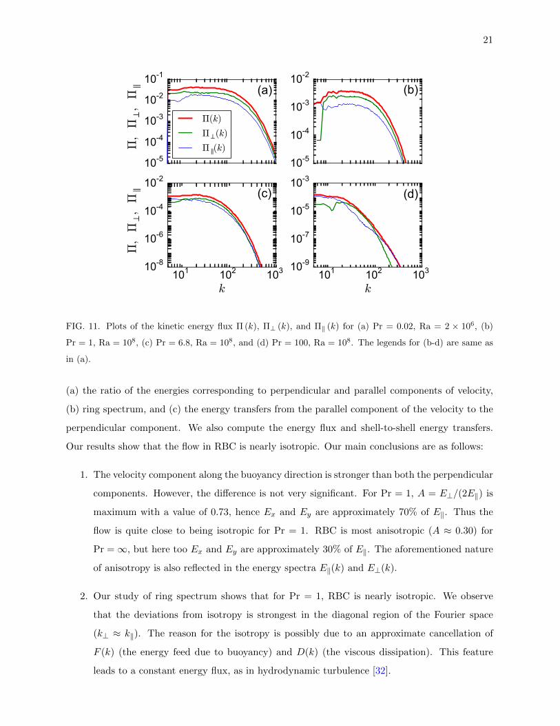
FIG. 11. Plots of the kinetic energy flux Π (k), Π⊥ (k), and Π‖ (k) for (a) Pr = 0.02, Ra = 2 × 10⁶, (b)
Pr = 1, Ra = 108, (c) Pr = 6.8, Ra = 108, and (d) Pr = 100, Ra = 108. The legends for (b-d) are same as
in (a).
(a) the ratio of the energies corresponding to perpendicular and parallel components of velocity,
(b) ring spectrum, and (c) the energy transfers from the parallel component of the velocity to the
perpendicular component. We also compute the energy flux and shell-to-shell energy transfers.
Our results show that the flow in RBC is nearly isotropic. Our main conclusions are as follows:
1. The velocity component along the buoyancy direction is stronger than both the perpendicular
components. However, the difference is not very significant. For Pr = 1, A = E⊥/(2E‖) is
maximum with a value of 0.73, hence Ex and Ey are approximately 70% of E‖. Thus the
flow is quite close to being isotropic for Pr = 1. RBC is most anisotropic (A ≈ 0.30) for
Pr =∞, but here too Ex and Ey are approximately 30% of E‖. The aforementioned nature
of anisotropy is also reflected in the energy spectra E‖(k) and E⊥(k).
2. Our study of ring spectrum shows that for Pr = 1, RBC is nearly isotropic. We observe
that the deviations from isotropy is strongest in the diagonal region of the Fourier space
(k⊥ ≈ k‖). The reason for the isotropy is possibly due to an approximate cancellation of
F (k) (the energy feed due to buoyancy) and D(k) (the viscous dissipation). This feature
leads to a constant energy flux, as in hydrodynamic turbulence [32].

22
10-4
10-2
0
-10-2
-10-4F,D,P
(a) (b)
101 102
k
10-4
10-2
0
-10-2
-10-4F,D,P
(c)101 102
k
(d)
F(k) D(k)
P (k)
FIG. 12. The energy supply rate by buoyancy F (k) (red curve), viscous dissipation rate D(k) (green curve),
and the energy transfer rate from u⊥ to u‖ via pressure, P‖(k) (blue stars) for (a) Pr = 0.02, Ra = 2× 10⁶,
(b) Pr = 1, Ra = 108, (c) Pr = 6.8, Ra = 108, and (d) Pr = 100, Ra = 108. The legends for (b–d) are same
as in (d).
3. For large and infinite Prandtl number, for which anisotropy is maximal, u⊥ is strong near
the polar region (ζ ≈ 0) of the Fourier space, while u‖ is strong near the equator (ζ ≈ π/2).
In this parameter regime, u‖ dominates u⊥, and it has a quasi-uniform structure along z;
these results are consistent with the features of thin plumes.
4. The reason for variation of anisotropy with Prandtl number is due to the plume structures.
For large and infinite Prandtl number RBC, the plumes are thin, and u‖ is stronger than u⊥,
consistent with the earlier observations by Hansen et al. [34]. The plumes tend to spread out
for lower Prandtl numbers. Still u‖ > u⊥ due to buoyancy. As a result A = E⊥/(2E‖) < 1
for all Prandtl numbers, but it monotonically decreases with the increase of the Prandtl
number.
5. We computed the shell-to-shell energy transfer among the shells in the Fourier space. We
show that the energy transfer is local and forward, very similar to that observed for hy-
drodynamic turbulence (in accordance to Kolmogorov’s theory). This is consistent with the
spectral studies of Kumar et al. [32] where they show that RBC exhibits Kolmogorov’s spec-
23
trum as in hydrodynamic turbulence. Our studies also show a small nonlocal energy transfer
from the third shell (corresponding to the large-scale convection rolls) to shells n = 4 to 10.
The energy flux is positive and constant in the inertial range, consistent with the forward and
local shell-to-shell energy transfers, a feature similar to that of hydrodynamic turbulence.
6. Buoyancy feeds energy to the parallel component of velocity, u‖. We show a net energy
transfer from u‖ to u⊥. This transfer, that occurs via pressure, maintains the steady state
of u⊥.
We remark that the anisotropy in RBC could depend on the boundary condition and geometry
(box or cylinder). Yet, the extent of anisotropy is expected to be approximately similar to the
results presented in this paper. This is because most of the energy of the flow resides in the bulk
(away from the boundary layer). The anisotropy studies in the boundary layer is beyond the scope
of this paper.
It is also important to compare anisotropy in various buoyancy-driven flows. In the present paper
we showed that for RBC, E⊥/(2E‖) varies from 0.30 (for Pr =∞) to 0.73 (for Pr = 1). Thus, RBC
is nearly isotropic for the range of Prandtl numbers from 0.02 to ∞. The other features such as
ring spectrum and shell-to-shell energy transfers also exhibit isotropy in RBC. The anisotropy in
Rayleigh-Taylor instability (RTI) varies with time during the growth of instability [24]. However in
the steady state, the behaviour of RTI is quite similar to RBC, e.g., E‖ is approximately three times
that of Ex [24]. Some of the anisotropy features of Unstably Stratified Homogeneous Turbulence
(USHT) are similar to that of RBC, albeit at smaller scales. In particular, Verma et al. [35] showed
that the Richardson number for RBC is Ri ≈ 16 leading to Froude number Fr = 1/√
Ri ≈ 0.25,
which is reasonably close to the saturated value of the Froude number of Burlot et al. [26] (see
Fig. 10 of Burlot et al. [26]).
Some of the tools discussed in the paper apply to other systems with external forcing, for
example, rotating turbulence [5], magnetohydrodynamic flows [4, 19], quasi-static magnetohydro-
dynamics [6–9, 21], and rotating convection [11]. Another notable and useful tool for studying
anisotropy is the toroidal and poloidal decomposition of the velocity field [5–8]. These studies
provide valuable insights into such flows, but more needs to be done, specially at high resolutions.
The present paper does not include discussion on the ring-to-ring energy transfers, as well as
on the entropy spectrum (|θ(k)|2) and entropy transfers for the temperature fluctuations. These
results will be presented in future. In this paper we detail the anisotropy in the whole fluid, which is
essentially dominated by the bulk flow. Quantification of anisotropy in the boundary layer will be
24
very useful for understanding and modelling the boundary layer. Thus we conclude our discussion
on the anisotropy quantification in RBC.
ACKNOWLEDGMENTS
We thank Biplab Dutta, Sandeep Reddy, Rohit Kumar, Anando Chatterjee, and J. K. Bhat-
tacharjee for useful discussions and help in postprocessing. This work was supported by re-
search grants from Indo-French Centre for the Promotion of Advanced Research (Grant No.
SPO/IFCPAR/PHY/20120319) and Science and Engineering Research Board, India (Grant num-
ber SERB/F/3279/2013-14). Our numerical simulations were performed on HPC cluster of IIT
Kanpur, Param Yuva at the Centre for Development of Advanced Computing (CDAC), and Sha-
heen supercomputer at KAUST supercomputing laboratory, Saudi Arabia.
[1] A. N. Kolmogorov, “Local structure of turbulence in incompressible viscous fluid for very large reynolds
number,” Dokl. Akad. Nauk SSSR, vol. 30, pp. 9–13, 1941.
[2] A. N. Kolmogorov, “Dissipation of energy in locally isotropic turbulence,” Dokl. Akad. Nauk SSSR,
vol. 32, pp. 16–18, 1941.
[3] A. N. Obukhov, “On the influence of archimedean forces on the structure of the temperature field in a
turbulent flow,” Dokl. Akad. Nauk SSSR, vol. 125, pp. 1246–1248, 1959.
[4] J. V. Shebalin, H. W. Matthaeus, and D. Montgomery, “Anisotropy in mhd turbulence due to a mean
magnetic field,” J. Plasma Physics, vol. 29, pp. 525–547, 1983.
[5] P. Sagaut and C. Cambon, Homogeneous Turbulence Dynamics. Cambridge University Press, 2008.
[6] B. Favier, F. S. Godeferd, and C. Cambon, “On space and time correlations of isotropic and rotating
turbulence,” Phys. Fluids, vol. 22, p. 015101, Jan 2010.
[7] B. Favier, F. S. Godeferd, C. Cambon, and A. Delache, “On the two-dimensionalization of quasistatic
magnetohydrodynamic turbulence,” Phys. Fluids, vol. 22, p. 075104, Jan 2010.
[8] B. Favier, F. S. Godeferd, C. Cambon, A. Delache, and W. J. T. Bos, “Quasi-static magnetohydrody-
namic turbulence at high reynolds number,” J. Fluid Mech., vol. 681, pp. 434–461, 8 2011.
[9] K. S. Reddy and M. K. Verma, “Strong anisotropy in quasi-static magnetohydrodynamic turbulence
for high interaction parameters,” Phys. Fluids, vol. 26, p. 025109, Feb 2014.
[10] F. Rincon, “Anisotropy, inhomogeneity and inertial-range scalings in turbulent convection,” J. Fluid
Mech., vol. 563, p. 43, Jan 2006.
[11] R. P. J. Kunnen, H. J. H. Clercx, and B. J. Geurts, “Enhanced vertical inhomogeneity in turbulent
rotating convection,” Phys. Rev. Lett., vol. 101, p. 174501, Oct 2008.

25
[12] D. Lohse and A. Muller-Groeling, “Anisotropy and scaling corrections in turbulence,” Phys. Rev. E,
vol. 54, pp. 395–405, Jul 1996.
[13] S. Kurien and K. R. Sreenivasan, “Anisotropic scaling contributions to high-order structure functions
in high-reynolds-number turbulence,” Phys. Rev. E, vol. 62, p. 2206, Aug 2000.
[14] L. Biferale and I. Procaccia, “Anisotropy in turbulent flows and in turbulent transport,” Phys. Rep.,
vol. 414, pp. 43–164, Jul 2005.
[15] L. Biferale, E. Calzavarini, A. S. Lanotte, F. Toschi, and R. Tripiccione, “Universality of anisotropic
turbulence,” Physica A, vol. 338, pp. 194–200, 2004.
[16] G. Ahlers, “Turbulent convection,” Physics, vol. 2, p. 74, Jan 2009.
[17] E. D. Siggia, “High rayleigh number convection,” Annu. Rev. Fluid Mech., vol. 26, p. 137, 1994.
[18] D. Lohse and K. Q. Xia, “Small-scale properties of turbulent rayleigh-benard convection,” Annu. Rev.
Fluid Mech., vol. 42, pp. 335–364, 2010.
[19] B. Teaca, M. K. Verma, B. Knaepen, and D. Carati, “Energy transfer in anisotropic magnetohydrody-
namic turbulence,” Phys. Rev. E, vol. 79, p. 046312, Jan 2009.
[20] A. Delache, C. Cambon, and F. Godeferd, “Scale by scale anisotropy in freely decaying rotating tur-
bulence,” Phys. Fluids, vol. 26, no. 2, 2014.
[21] K. S. Reddy, R. Kumar, and M. K. Verma, “Anisotropic energy transfers in quasi-static magnetohy-
drodynamic turbulence,” Phys. Plasmas, vol. 21, p. 102310, Oct 2014.
[22] M. Chertkov, “Phenomenology of rayleigh-taylor turbulence,” Phys. Rev. Lett., vol. 91, p. 115001, Sep
2003.
[23] G. Boffetta, F. De Lillo, A. Mazzino, and S. Musacchio, “Bolgiano scale in confined rayleigh–taylor
turbulence,” J. Fluid Mech., vol. 690, pp. 426–440, 1 2012.
[24] W. Cabot and Y. Zhou, “Statistical measurements of scaling and anisotropy of turbulent flows induced
by Rayleigh-Taylor instability,” Phys. Fluids, vol. 25, no. 1, pp. 015107–19, 2013.
[25] O. Soulard, J. Griffond, and B.-J. Grea, “Large-scale analysis of self-similar unstably stratified homo-
geneous turbulence,” Phys. Fluids, vol. 26, no. 1, 2014.
[26] A. Burlot, B.-J. Grea, F. S. Godeferd, C. Cambon, and J. Griffond, “Spectral modelling of high reynolds
number unstably stratified homogeneous turbulence,” J. Fluid Mech., vol. 765, no. 17, 2015.
[27] S. Chandrasekhar, Hydrodynamic and Hydromagnetic Stability. New York: Dover Publications, 1961.
[28] S. B. Pope, Turbulent Flows. Cambridge University Press, 2000.
[29] G. Dar, M. Verma, and V. Eswaran, “Energy transfer in two-dimensional magnetohydrodynamic tur-
bulence: formalism and numerical results,” Physica D, vol. 157, pp. 207–225, Jan 2001.
[30] M. K. Verma, “Statistical theory of magnetohydrodynamic turbulence: Recent results,” Phys. Rep.,
vol. 401, pp. 229–380, 2004.
[31] M. K. Verma, A. G. Chatterjee, K. S. Reddy, R. K. Yadav, S. Paul, M. Chandra, and R. Samtaney,
“Benchmarking and scaling studies of a pseudospectral code tarang for turbulence simulations,” Pra-
mana, vol. 81, pp. 617–629, 2013.

26
[32] A. Kumar, A. G. Chatterjee, and M. K. Verma, “Energy spectrum of buoyancy-driven turbulence,”
Phys. Rev. E, vol. 90, p. 023016, Aug 2014.
[33] A. Pandey, M. K. Verma, and P. K. Mishra, “Scaling of heat flux and energy spectrum for very large
prandtl number convection,” Phys. Rev. E, vol. 89, p. 023006, Feb 2014.
[34] U. Hansen, D. A. Yuen, and S. E. Kroening, “Transition to hard turbulence in thermal convection at
infinite prandtl number,” Phys. Fluids, vol. 2, p. 2157, 1990.
[35] M. K. Verma, A. Kumar, and A. G. Chatterjee, “Energy spectrum and flux of buoyancy-driven tur-
bulence,” in: Advances in Computation, Modeling and Control of Transitional and Turbulent Flows,
World Scientific, 2016.