Embed Size (px)
Citation preview
7/31/2019 Nea Study of Thermal Fatigue
http://slidepdf.com/reader/full/nea-study-of-thermal-fatigue 1/147
For Official Use NEA/CSNI/R(2005)2 Organisation de Coopération et de Développement EconomiquesOrganisation for Economic Co-operation and Development 01-Aug-2005
___________________________________________________________________________________________ English text only
NUCLEAR ENERGY AGENCYCOMMITTEE ON THE SAFETY OF NUCLEAR INSTALLATIONS
CSNI INTEGRITY AND AGEING WORKING GROUP
FAT3D- An OECD/NEA benchmark on thermal fatigue in fluid mixing areas
The complete document is only available in pdf format.
NEA
/ C S NI
/ R ( 2 0 0 5 ) 2
F or
Of f i c i al U
s e Cancels & replaces the same document of 29 July 2005
7/31/2019 Nea Study of Thermal Fatigue
http://slidepdf.com/reader/full/nea-study-of-thermal-fatigue 2/147
NEA/CSNI/R(2005)2
ORGANISATION FOR ECONOMIC CO-OPERATION AND DEVELOPMENT
Pursuant to Article 1 of the Convention signed in Paris on 14th December 1960, and which came into force on 30thSeptember 1961, the Organisation for Economic Co-operation and Development (OECD) shall promote policies designed:
• to achieve the highest sustainable economic growth and employment and a rising standard of living in member countries, while maintaining financial stability, and thus to contribute to the development of the world economy;
• to contribute to sound economic expansion in member as well as non-member countries in the process of economicdevelopment; and
• to contribute to the expansion of world trade on a multilateral, non-discriminatory basis in accordance withinternational obligations.
The original member countries of the OECD are Austria, Belgium, Canada, Denmark, France, Germany, Greece, Iceland,Ireland, Italy, Luxembourg, the Netherlands, Norway, Portugal, Spain, Sweden, Switzerland, Turkey, the United Kingdom and theUnited States. The following countries became members subsequently through accession at the dates indicated hereafter: Japan(28th April 1964), Finland (28th January 1969), Australia (7th June 1971), New Zealand (29th May 1973), Mexico (18th May1994), the Czech Republic (21st December 1995), Hungary (7th May 1996), Poland (22nd November 1996), Korea (12thDecember 1996) and the Slovak Republic (14 December 2000). The Commission of the European Communities takes part in thework of the OECD (Article 13 of the OECD Convention).
NUCLEAR ENERGY AGENCY
The OECD Nuclear Energy Agency (NEA) was established on 1st February 1958 under the name of the OEEC European Nuclear Energy Agency. It received its present designation on 20th April 1972, when Japan became its first non-European fullmember. NEA membership today consists of 28 OECD member countries: Australia, Austria, Belgium, Canada, the CzechRepublic, Denmark, Finland, France, Germany, Greece, Hungary, Iceland, Ireland, Italy, Japan, Luxembourg, Mexico, the Netherlands, Norway, Portugal, Republic of Korea, the Slovak Republic, Spain, Sweden, Switzerland, Turkey, the UnitedKingdom and the United States. The Commission of the European Communities also takes part in the work of the Agency.
The mission of the NEA is:
• to assist its member countries in maintaining and further developing, through international co-operation, thescientific, technological and legal bases required for a safe, environmentally friendly and economical use of nuclear energy for peaceful purposes, as well as
• to provide authoritative assessments and to forge common understandings on key issues, as input to governmentdecisions on nuclear energy policy and to broader OECD policy analyses in areas such as energy and sustainabledevelopment.
Specific areas of competence of the NEA include safety and regulation of nuclear activities, radioactive wastemanagement, radiological protection, nuclear science, economic and technical analyses of the nuclear fuel cycle, nuclear law andliability, and public information. The NEA Data Bank provides nuclear data and computer program services for participatingcountries.
7/31/2019 Nea Study of Thermal Fatigue
http://slidepdf.com/reader/full/nea-study-of-thermal-fatigue 3/147
NEA/CSNI/R(2005)2
COMMITTEE ON THE SAFETY OF NUCLEAR INSTALLATIONS
The NEA Committee on the Safety of Nuclear Installations (CSNI) is an international committee made up of senior scientistsand engineers, with broad responsibilities for safety technology and research programmes, and representatives from regulatoryauthorities. It was set up in 1973 to develop and co-ordinate the activities of the NEA concerning the technical aspects of thedesign, construction and operation of nuclear installations insofar as they affect the safety of such installations.
The committee’s purpose is to foster international co-operation in nuclear safety amongst the OECD member countries. TheCSNI’s main tasks are to exchange technical information and to promote collaboration between research, development,engineering and regulatory organisations; to review operating experience and the state of knowledge on selected topics of nuclear safety technology and safety assessment; to initiate and conduct programmes to overcome discrepancies, develop improvementsand research consensus on technical issues; to promote the coordination of work that serve maintaining competence in the nuclear safety matters, including the establishment of joint undertakings.
The committee shall focus primarily on existing power reactors and other nuclear installations; it shall also consider the safetyimplications of scientific and technical developments of new reactor designs.
In implementing its programme, the CSNI establishes co-operative mechanisms with NEA’s Committee on Nuclear Regulatory Activities (CNRA) responsible for the program of the Agency concerning the regulation, licensing and inspection of nuclear installations with regard to safety. It also co-operates with NEA’s Committee on Radiation Protection and Public Health(CRPPH), NEA’s Radioactive Waste Management Committee (RWMC) and NEA’s Nuclear Science Committee (NSC) onmatters of common interest.

7/31/2019 Nea Study of Thermal Fatigue
http://slidepdf.com/reader/full/nea-study-of-thermal-fatigue 4/147
NEA/CSNI/R(2005)2
7/31/2019 Nea Study of Thermal Fatigue
http://slidepdf.com/reader/full/nea-study-of-thermal-fatigue 5/147
NEA/CSNI/R(2005)2
FOREWORD
At the CSNI meeting in June 2002, the proposal for a benchmark on thermal fatigue in fluid mixingareas based on the test performed by CEA, France was approved. Objectives were to extend theunderstanding of 3D thermo mechanical loading as a major factor influencing crack propagation throughthe thickness of nuclear piping systems. The benchmark was sponsored by IRSN.
This report presents the analysis results of the calculation of the experiment provided by the benchmark participants.
The CSNI Working Group on the Integrity and Ageing and in particular its sub-group on the integrityof metal components has produced extensive material over the last few years. In the area of thermalfatigue, it has recently produced the following material:
1. Thermal cycling in LWR components in OECD-NEA member countries (NEA/CSNI/R(2005)8) -Review of operating experience, regulatory framework, countermeasures and current research;
2. This benchmark;3. Organization with the EPRI and the USNRC of the international conference on fatigue of reactor
components. This conference reviews progress in the areas and provides a forum for discussionand exchange of information between high level experts. The conference is held every other year to follow the progress and to direct research to key aspects. The last edition was held on October 3-6, 2004.
In addition a large number of NEA member countries are participating in the OECD Piping FailureData Exchange Project (OPDE) to collect field experience on piping degradation.
The complete list of CSNI reports, and the text of reports from 1993 onwards, is available onhttp://www.nea.fr/html/nsd/docs/

7/31/2019 Nea Study of Thermal Fatigue
http://slidepdf.com/reader/full/nea-study-of-thermal-fatigue 6/147
NEA/CSNI/R(2005)2
7/31/2019 Nea Study of Thermal Fatigue
http://slidepdf.com/reader/full/nea-study-of-thermal-fatigue 7/147

7/31/2019 Nea Study of Thermal Fatigue
http://slidepdf.com/reader/full/nea-study-of-thermal-fatigue 8/147
NEA/CSNI/R(2005)2
7/31/2019 Nea Study of Thermal Fatigue
http://slidepdf.com/reader/full/nea-study-of-thermal-fatigue 9/147
NEA/CSNI/R(2005)2
EXECUTIVE SUMMARY
Thermal cycling is a widespread and recurring problem in nuclear power plants worldwide. Severalincidents with leakage of primary water inside the containment challenged the integrity of nuclear power plants although no release outside of containment occurred. Thermal cycling was not taken into account atthe design stage. Regulatory bodies, utilities and researchers have to address it for their operating plants. Itis a complex phenomenon that involves and links thermal hydraulic, fracture mechanic, materials and plantoperation.
Thermal fatigue in a fluid mixing area is a well-known phenomenon that has already been studied inthe past. Generally, this phenomenon is linked to turbulent mixing of two fluids at two differenttemperatures and creates “elephant skin” type damage at the inner surface of the component and somecracks, which remain relatively small, compared to the thickness of the structure.
However, as was the case for a tee junction of the French Super Phenix fast breeder reactor (chosenconfiguration for an international benchmark study [1]) and more recently for a pressurized water reactor atCivaux nuclear power plant [2], this kind of fatigue damage can create cracks that propagate through theentire wall thickness.
Some experts consider that 3D thermo mechanical loading is a major factor influencing crack propagation through the thickness. This factor is linked to the complex thermal hydraulic loading and has
an impact on the stress distribution in the structure and the damage or crack propagation estimates. For thisreason an R&D program, based on a test and numerical interpretations, was launched by IRSN andconducted by CEA to quantify experimentally the influence of the 3D aspects on crack initiation and propagation. The main objective was to work on a configuration with a 3D thermal load easy enough toreproduce using numerical simulations, so that accurate mechanical studies could be carried out andassessment methodologies be validated or modified.
Under the auspices of the OECD/NEA Committee for the Safety of Nuclear Installations (CSNI) andits Working Group on Integrity of Components and Structures (IAGE), a benchmark was launched in 2002.Seven organisations from 4 countries contributed to this effort aiming at comparing different approachesused for mechanical assessment of this 3D configuration.
Organised in three major steps, the benchmark included the definition, the realisation and the analysisof a test on fatigue crack propagation under pure thermal loading in which important cracking, untilpenetration was observed
7/31/2019 Nea Study of Thermal Fatigue
http://slidepdf.com/reader/full/nea-study-of-thermal-fatigue 10/147
NEA/CSNI/R(2005)2
Due to a movement of the cooling pipe at the beginning of the test, the thermal loading was moresevere than the loading characterised with the thermal mock-up. It was thus difficult to comparequantitatively the prediction of participants with the experiment.
However, a qualitative comparison showed that predictions were in good agreement with test results:
- The location and the orientation of the cracks were predicted by the participants: due to circumferentialstresses, axial cracks were dominant at the bottom of the cooling area;
-Cracks propagation through the thickness was predicted and, for all participants, the number of cyclesto go through wall was close to the number of cycles for initiation. This was in agreement with the test(i.e. 12000 cycles to initiate a crack and 17500 for the complete penetration).
Post interpretation made with corrected thermal loading showed that crack initiation happened belowthe fatigue best fit curve of the material. This result needs to be confirmed with complementary tests andanalyses.
7/31/2019 Nea Study of Thermal Fatigue
http://slidepdf.com/reader/full/nea-study-of-thermal-fatigue 11/147
NEA/CSNI/R(2005)2
TABLE OF CONTENTS
1. INTRODUCTION – OBJECTIVES OF THE BENCHMARK.........................................................132. BENCHMARK ORGANISATION....................................................................................................143. TEST DESCRIPTION: THE FAT3D EXPERIMENT......................................................................15
3.1 Material data ...................................................................................................................................163.2 Mock-up geometry..........................................................................................................................16
3.3 Boundary conditions .......................................................................................................................163.4 Load description..............................................................................................................................173.4.1 Thermal loading optimization ...............................................................................................183.4.2 Qualification of the thermal loading......................................................................................183.4.3 Characterization of the surface in contact with water ...........................................................20
4. OBJECTIVE OF THE BENCHMARK ..............................................................................................224.1 Main objectives ...............................................................................................................................22
4.2 Expected tests results ......................................................................................................................224.3 Pre test calculation ..........................................................................................................................224.4 Blind test analysis ...........................................................................................................................234.5 Synthesis and discussion.................................................................................................................23
5. MAIN RESULTS AND CONCLUSIONS FROM THE PRE TEST ANALYSES............................245.1 Preliminary questions......................................................................................................................245.2 Participants......................................................................................................................................245.3 Synthesis of the main results...........................................................................................................24
6. MAIN RESULTS AND CONCLUSIONS FROM THE BLIND TEST ANALYSIS........................256.1 Participants and models used ..........................................................................................................256.2 Models used ....................................................................................................................................256.3 Calibration of the thermal model ....................................................................................................256.4 Elastic stress analysis ......................................................................................................................26

7/31/2019 Nea Study of Thermal Fatigue
http://slidepdf.com/reader/full/nea-study-of-thermal-fatigue 12/147
NEA/CSNI/R(2005)2
Measurements for θ = 0°............................................................................................................................36Measurements for θ = 20°..........................................................................................................................37Measurements for θ = 40°..........................................................................................................................38Measurements for θ= 70°...........................................................................................................................39Appendix II: Participant contributions.......................................................................................................40
7/31/2019 Nea Study of Thermal Fatigue
http://slidepdf.com/reader/full/nea-study-of-thermal-fatigue 13/147
NEA/CSNI/R(2005)2
1. INTRODUCTION – OBJECTIVES OF THE BENCHMARK
Thermal fatigue in high flow mixing areas is a longstanding problem. In these areas of high flow rateand extensive discontinuities, the mixture becomes turbulent and a wide range of turbulence frequenciesand thermal fluctuations are encountered. The consequence for structures is multiple or isolated crackswhich, in some cases, may not be very deep but which in others can cause perforation of the structure.
A highly complicated issue is why some configurations have more capacities than others to withstandthermal stresses and why multiple cracks should occur in some places and isolated cracks in others. Manytest results are available and R&D programs are currently being carried out to supplement them.
Some experts consider that these phenomenons may be attributed to the fact that the 3D aspect of thermal loading is becoming predominant in certain flow configurations. These overall thermal loads resultin complex 3D mechanical loads involving the entire thickness of a component. Generally speaking, verylittle is known about the thermo hydraulic and thermo mechanical aspects of these loads when they occur in complex structures such as mixing tees. For this reason an R&D program, based on a test and numericalinterpretations, was launched to quantify experimentally the influence of the 3D aspects on crack initiationand propagation. The program was intended to clarify and illustrate the problem of overall thermal loadingand to suggest tools that would enable it to be taken into account at the design stage [6]. It included bothlaboratory experiments and numerical analyses using the applied loads.
Under the auspices of the OECD/NEA Committee for the Safety of Nuclear Installations (CSNI) and
its Working Group on Integrity of Components and Structures (IAGE), a benchmark was launched in 2002.Seven organisations from 4 countries contributed to this effort aiming at comparing different approachesused for mechanical assessment of this 3D configuration.
Main idea of the benchmark was to use a simple laboratory configuration as a basis for comparing andexchanging know-how and highlighting important physical parameters. It was organized in three major steps:
• Participant approaches were applied to the test design with a view to specifying the test objectives andhow the results would be presented and discussed,
• Approaches were applied to the forecast outcome of the test so that they could be compared withobservations made in the laboratory,
• A discussion and synthesis reports.
This report constitutes the synthesis phase of the benchmark It describes the different phases of the
7/31/2019 Nea Study of Thermal Fatigue
http://slidepdf.com/reader/full/nea-study-of-thermal-fatigue 14/147
NEA/CSNI/R(2005)2
2. BENCHMARK ORGANISATION
The benchmark was organised using the CEA - FAT3D experiment. However, because the test wasstill at a design level when this benchmark started, it was proposed to the OECD/NEA/CSNI/IAGEworking group members to participate in the test definition. The proposed experimental approach was thefollowing:
• Preliminary calculations : the aim of this stage is to determine the experimental possibilities of the testapparatus and establish the temperatures and cycle durations to be used etc. This is the first stage of the benchmark study.
• Characterisation of the thermal loading : knowledge of the thermal loading imposed on the structure isa very important aspect of the problem. It is therefore determined accurately using a thermal mock-up provided with temperature measurements on the surface and through the thickness.
• Blind test analysis. The aim of this stage is to predict cracking of the specimen with a known thermalload. This is the second stage of the benchmark study for validating the various methods.
• The thermo mechanical test takes place concurrently with this calculation stage. The tests results arenot sent to the participants during the calculation stage.
• Comparison of results: the results obtained by all the participants are collected and compared with thetest results and discussed at a meeting of OECD work group IAGE.
• Synthesis of the benchmark. The objective at this stage is to highlight main results obtained and propose some general conclusions on the way to take into account 3D thermal loadings in structuralintegrity analyses.This three years effort was divided as follows:
January 2002 September 2002: Preliminary test calculations (all participants )September 2002 December 2002: Analysis of preliminary calculations (CEA)January 2003 February 2003: Thermal tests (CEA)March 2003 September 2003: Assessment of damage (all participants )March 2003 December 2003: Test (CEA)January 2004 April 2004: Analysis of results (CEA)June 2004: Conclusions and discussions (all participants )December 2004: Synthesis
7/31/2019 Nea Study of Thermal Fatigue
http://slidepdf.com/reader/full/nea-study-of-thermal-fatigue 15/147
NEA/CSNI/R(2005)2
3. TEST DESCRIPTION: THE FAT3D EXPERIMENT
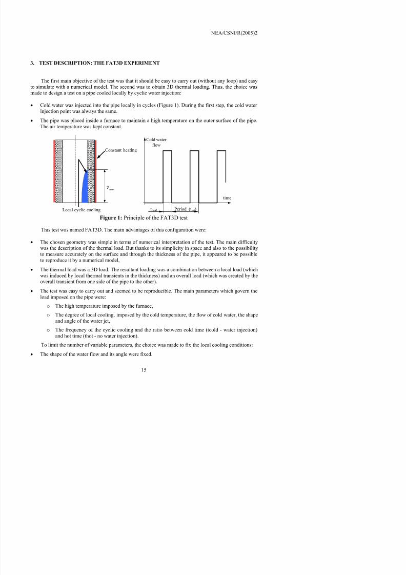
The first main objective of the test was that it should be easy to carry out (without any loop) and easyto simulate with a numerical model. The second was to obtain 3D thermal loading. Thus, the choice wasmade to design a test on a pipe cooled locally by cyclic water injection:
• Cold water was injected into the pipe locally in cycles (Figure 1). During the first step, the cold water injection point was always the same.
• The pipe was placed inside a furnace to maintain a high temperature on the outer surface of the pipe.The air temperature was kept constant.
Zmax
Local cyclic cooling
Constant heating
time
Cold water flow
tcold Period (ttot)
Figure 1: Principle of the FAT3D test
This test was named FAT3D. The main advantages of this configuration were:
• The chosen geometry was simple in terms of numerical interpretation of the test. The main difficultywas the description of the thermal load. But thanks to its simplicity in space and also to the possibilityto measure accurately on the surface and through the thickness of the pipe, it appeared to be possibleto reproduce it by a numerical model,
• The thermal load was a 3D load. The resultant loading was a combination between a local load (whichwas induced by local thermal transients in the thickness) and an overall load (which was created by theoverall transient from one side of the pipe to the other).
7/31/2019 Nea Study of Thermal Fatigue
http://slidepdf.com/reader/full/nea-study-of-thermal-fatigue 16/147
NEA/CSNI/R(2005)2
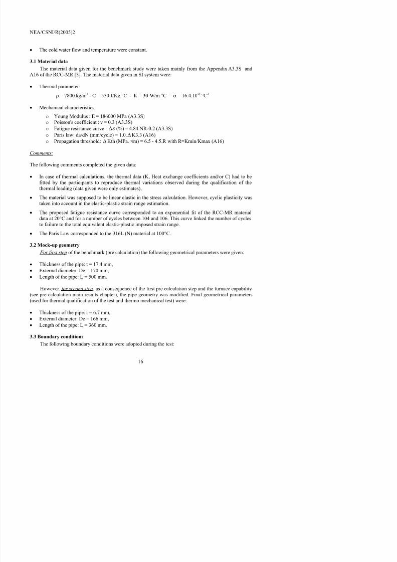
• The cold water flow and temperature were constant.3.1 Material data
The material data given for the benchmark study were taken mainly from the Appendix A3.3S andA16 of the RCC-MR [3]. The material data given in SI system were:
• Thermal parameter:ρ = 7800 kg/m3 - C = 550 J/Kg.°C - K = 30 W/m.°C -α = 16.4.10-6 °C-1
• Mechanical characteristics:o Young Modulus : E = 186000 MPa (A3.3S)o Poisson's coefficient : ν = 0.3 (A3.3S)o Fatigue resistance curve :ε ∆ (%) = 4.84.NR-0.2 (A3.3S)o Paris law: da/dN (mm/cycle) = 1.0.∆K3.3 (A16)o Propagation threshold:∆Kth (MPa.√m) = 6.5 - 4.5.R with R=Kmin/Kmax (A16)
Comments:
The following comments completed the given data:
• In case of thermal calculations, the thermal data (K, Heat exchange coefficients and/or C) had to befitted by the participants to reproduce thermal variations observed during the qualification of thethermal loading (data given were only estimates),
• The material was supposed to be linear elastic in the stress calculation. However, cyclic plasticity wastaken into account in the elastic-plastic strain range estimation.• The proposed fatigue resistance curve corresponded to an exponential fit of the RCC-MR material
data at 20°C and for a number of cycles between 104 and 106. This curve linked the number of cyclesto failure to the total equivalent elastic-plastic imposed strain range.
• The Paris Law corresponded to the 316L (N) material at 100°C.
3.2 Mock-up geometry For first step of the benchmark (pre calculation) the following geometrical parameters were given:
• Thickness of the pipe: t = 17.4 mm,• External diameter: De = 170 mm,• Length of the pipe: L = 500 mm.
7/31/2019 Nea Study of Thermal Fatigue
http://slidepdf.com/reader/full/nea-study-of-thermal-fatigue 17/147
NEA/CSNI/R(2005)2
• The section at the top of the pipe was supposed to be embedded.• The section at the bottom of the pipe (where water goes out from the pipe) was free.
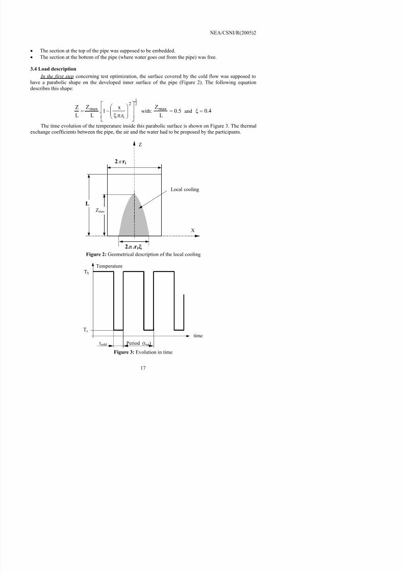
3.4 Load description In the first step concerning test optimization, the surface covered by the cold flow was supposed to
have a parabolic shape on the developed inner surface of the pipe (Figure 2). The following equationdescribes this shape:
212
imax
r ..x1.
LZ
LZ
πξ−= with: 5.0
LZmax = and 4.0=ξ
The time evolution of the temperature inside this parabolic surface is shown on Figure 3. The thermalexchange coefficients between the pipe, the air and the water had to be proposed by the participants.
X
Z
Local cooling
2 π r i
Zmax
L
2. .r i. Figure 2: Geometrical description of the local cooling
TemperatureTh
7/31/2019 Nea Study of Thermal Fatigue
http://slidepdf.com/reader/full/nea-study-of-thermal-fatigue 18/147
NEA/CSNI/R(2005)2
In second step , the thermal cycle was optimized. The thermal loading amplitude and the boundary of the cold water flow on the internal surface were measured on a specific mock up. Results are described inthe thermal qualification chapter and in appendix I.
3.4.1 Thermal loading optimization
During the test design, a preliminary thermal loading optimization was performed. Finally, theoptimized cycle was defined by:
• Water temperature : Tcold ~ 17 – 20°C• Furnace temperature : Thot = 650°C• Total cycle duration : ttot = tcold + thot = 190 s• Water injection time : tcold = 15 s
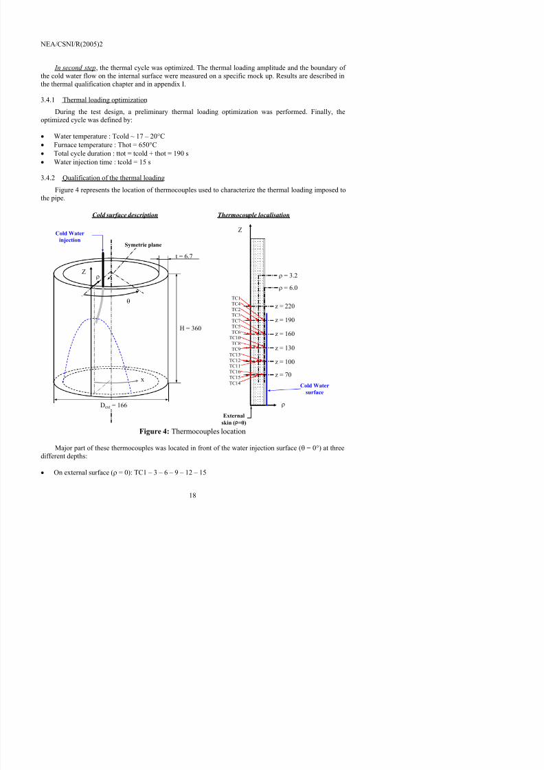
3.4.2 Qualification of the thermal loadingFigure 4 represents the location of thermocouples used to characterize the thermal loading imposed to
the pipe.
Cold Waterinjection
Symetrie plane
Z
x
ρ
H = 360
t = 6.7
Z
z = 70
z = 100
z = 130
z = 160
z = 190
z = 220
ρ = 6.0
ρ = 3.2
TC1TC4TC2TC3TC7TC5TC6
TC10TC8TC9
TC13TC12TC11TC16TC15TC14
Cold surface description Thermocouple localisation
θ
7/31/2019 Nea Study of Thermal Fatigue
http://slidepdf.com/reader/full/nea-study-of-thermal-fatigue 19/147
NEA/CSNI/R(2005)2
• At a 3.2 mm depth : TC2 – 5 – 8 – 11 – 14• Close to the inner surface (ρ= 6,1 mm) : TC4 – 7 – 10 – 13 – 16
At the opposite of the pipe (θ = 180°), 3 thermocouples were located on the external surface (ρ = 0):TC17 – 18 – 19. In addition, the mock-up would rotate so that measurements would be performed outsidethe symmetry plane of the water injection: the mock up could rotate for an angleθ which could vary from0 to 70°.
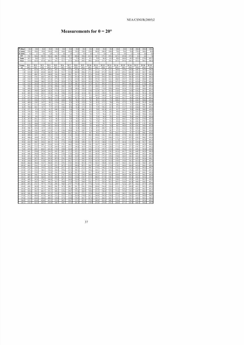
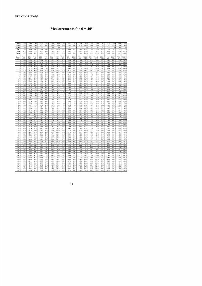
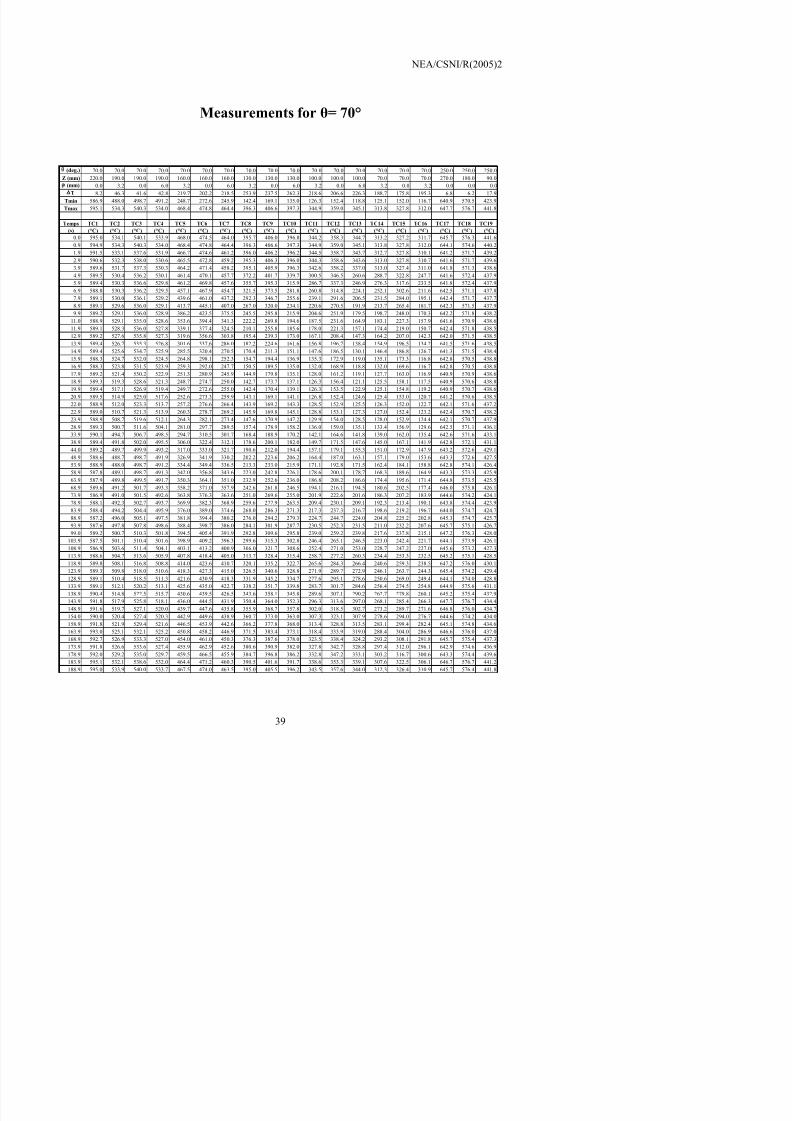
All the measurements performed during the thermal test were given in appendix I. It concerned theevolution with time of the temperature measured by each thermocouple (19 TC), for the stabilized cycleand for four angle positions:θ = 0 – 20 – 40 – 70°.
The next figures showed some examples of temperature variation with time:
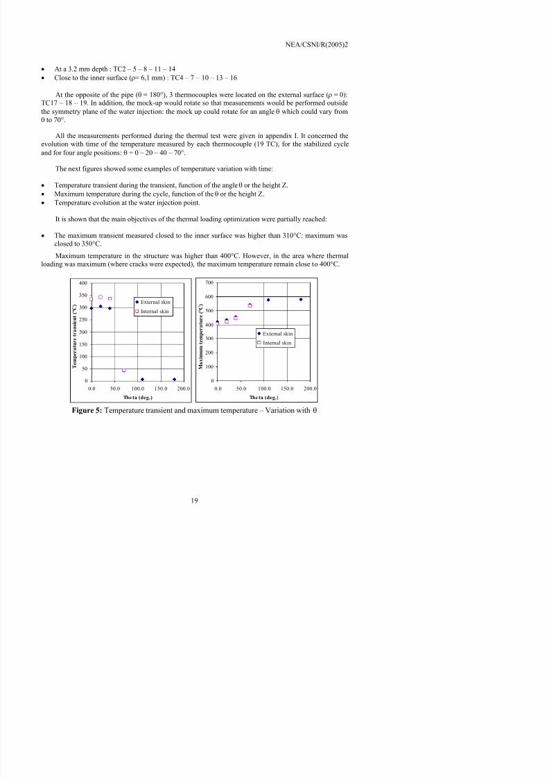
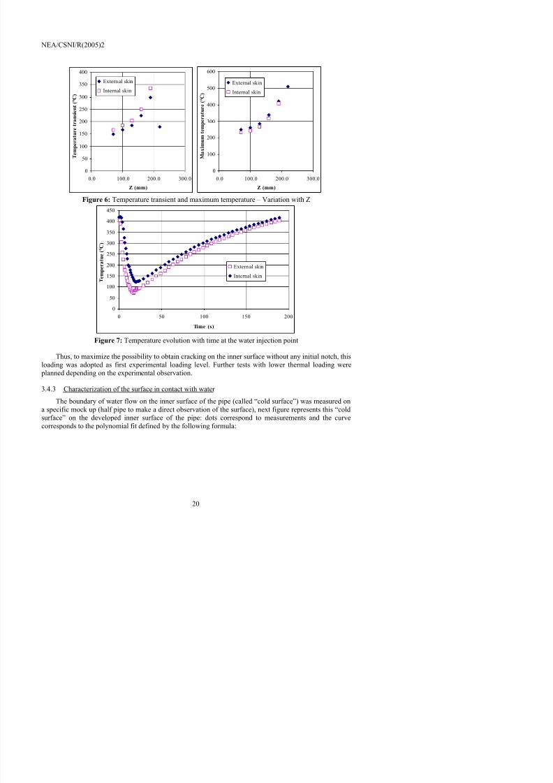
• Temperature transient during the transient, function of the angleθ or the height Z.• Maximum temperature during the cycle, function of theθ or the height Z.
•
Temperature evolution at the water injection point.It is shown that the main objectives of the thermal loading optimization were partially reached:
• The maximum transient measured closed to the inner surface was higher than 310°C: maximum wasclosed to 350°C.Maximum temperature in the structure was higher than 400°C. However, in the area where thermal
loading was maximum (where cracks were expected), the maximum temperature remain close to 400°C.
0
50
100
150
200
250
300
350
400
T e m p e r a t u r e
t r a n s i e n t ( ° C ) External skin
Internal skin
0
100
200
300
400
500
600
700
M a x i m u m
t e m p e r a t u r e
( ° C )
External skin
Internal skin
7/31/2019 Nea Study of Thermal Fatigue
http://slidepdf.com/reader/full/nea-study-of-thermal-fatigue 20/147
NEA/CSNI/R(2005)2
0
50
100
150
200
250
300
350
400
0.0 100.0 200.0 300.0Z (mm)
T e m p e r a
t u r e t r a n s i e n t ( ° C )
External skinInternal skin
0
100
200
300
400
500
600
0.0 100.0 200.0 300.0Z (mm)
M a x i m u m
t e m p e r a t u r e
( ° C )
External skinInternal skin
Figure 6: Temperature transient and maximum temperature – Variation with Z
0
50
100150
200
250
300
350
400
450
0 50 100 150 200
Time (s)
T e m
p e r a t u e ( ° C )
External skin
Internal skin
Figure 7: Temperature evolution with time at the water injection point
Thus, to maximize the possibility to obtain cracking on the inner surface without any initial notch, thisloading was adopted as first experimental loading level. Further tests with lower thermal loading were planned depending on the experimental observation.
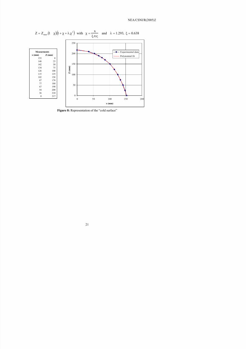
3 4 3 Characterization of the surface in contact with water
7/31/2019 Nea Study of Thermal Fatigue
http://slidepdf.com/reader/full/nea-study-of-thermal-fatigue 21/147
NEA/CSNI/R(2005)2
( )( ) 0.638 ,293.1 and r ..xwith.1.1.ZZi
3max =ξ=λπξ=χχλ+χ+χ−=
0
50
100
150
200
250
0 50 100 150 200
(mm)
Z ( m m
)
Experimental dataPolynomial fit(mm) Z (mm)
153 0
148 25142 50134 75126 100115 125102 15087 17077 18067 19054 20036 2100 217
Measurments
x (mm)
x (mm)
Figure 8: Representation of the “cold surface”
7/31/2019 Nea Study of Thermal Fatigue
http://slidepdf.com/reader/full/nea-study-of-thermal-fatigue 22/147
NEA/CSNI/R(2005)2
4. OBJECTIVE OF THE BENCHMARK
4.1 Main objectivesThe main objectives of the benchmark were to compare assessment procedures for the evaluation of
fatigue cracking under thermal load:
• How to evaluate the thermal load on the structure? What were the most important parameters on the
mechanical loading and the fatigue damage?• How to evaluate cracking? In terms of crack initiation or crack propagation?
The experimental support represented one of the main interests of the proposed exercise, because itallowed quantifying the quality of the proposed methodologies. However, one had to remember that thistest did not cover all the technical problems linked to thermal fatigue topics, but only a small aspectcorresponding to the 3D thermal loading. Other themes such as high cycle fatigue or random loadingscould not be studied with the proposed test.
4.2 Expected tests resultsThe objective of the design test was to analyze cracking in a pipe under cyclic loading, in terms of
crack initiation and propagation. However, this test had to respect the following conditions:
• In terms of duration: the test had to remain in a reasonable time (between 3 and 6 month)• In terms of temperature: the hot temperature had to remain below 400°C to avoid creep damage in the
pipe and important variations of material characteristics with temperature.The cold thermal shock conditions being fixed, the main parameters which were to be defined in
acceptance with these two experimental objectives were the hot temperature (temperature of the furnace),the frequency of the thermal cycles and the proportion between cold time and the period (τ = tcold / ttot – Figure 1).
4.3 Pre test calculationThe first step was devoted to the pre calculation of the test. At this level, it was asked to the
participants to propose an integrity assessment procedure and to use it to optimize the test conditions:
• A description of the employed assessment procedure and the assumptions made to apply it on the proposed configuration were asked to the participants (thermal load evaluation, stresses and strainscalculation, damage evaluation…). The comparison of the different choices was one of the firstinteresting results of this benchmark.
7/31/2019 Nea Study of Thermal Fatigue
http://slidepdf.com/reader/full/nea-study-of-thermal-fatigue 23/147
NEA/CSNI/R(2005)2
o Shape ratio (crack depth over half length): a/c = 1/3.The only parameter which had to be determined is the initial relative crack depth a/t.
4.4 Blind test analysisBlind test analysis had consisted of the interpretation of the thermo mechanical test. This step is
composed of three major stages:
• The definition of the complete thermal load solicitation: from the measurement made on the thermal
specimen, a description of the thermal load imposed by the water at the inner surface had to bedefined. This stage was mainly performed by a numerical analysis (3D or more simple 1D analysis)and consisted of the precise determination of the imposed temperature to the structure and of thethermal data of the problem (heat exchange coefficients, conductivity…). The definition of the thermalfield in the pipe was deduced from this calculation.
• Knowing the thermal field, the stress and strain fields are determined in the pipe. An analysis of thesefields was then performed:
o Local analysis: evolution of stresses and strains with time, stress on the inner surface,membrane and bending stresses…
o Global analysis: mean stresses on the pipe…• Following the stress and strain analysis, the damage analysis or the crack propagation analyses were
performed.The numbers of cycles to crack initiation on the inner surface and crack propagation celerity through
the thickness of the pipe (for a given number of cycles) were the main required results that were comparedwith the test.
4.5 Synthesis and discussionA synthesis of the different proposed assessment procedures and a comparison of the different
assumptions and results obtained were prepared.This synthesis was presented to the partners and then discussed [7]. At this level, some perspectives
on structural assessment under 3D thermal fatigue loading were proposed by the participants of the benchmark.
7/31/2019 Nea Study of Thermal Fatigue
http://slidepdf.com/reader/full/nea-study-of-thermal-fatigue 24/147
NEA/CSNI/R(2005)2
5. MAIN RESULTS AND CONCLUSIONS FROM THE PRE TEST ANALYSES
5.1 Preliminary questionsA series of questions was sent to CEA by participants before the analysis. These questions or
comments mainly concerned the understanding of the thermal loading, the material data… All questionsfrom participants and replies from CEA are given in the second step proposal [5].
5.2 ParticipantsFour contributions were received for this first step, including global 3D thermo mechanical analysisand 1D analytical estimations. Participants were:
• JNC – JOYO – CRC (Japan) which proposed an analytical approach called “cold spot approach”which allowed taking into account structural effects in 1D thermal approach.
• Vamet (Czech Republic), DNV (Sweden) and CEA (France) which proposed a complete 3D massivethermo mechanical analysis.
5.3 Synthesis of the main resultsMain results obtained from the analysis are the following:
• From 3D calculations and for the given thermal conditions in the first step for the pre test analysis,stress level was not important enough to reach crack initiation in a reasonable time on the inner surface.
•
1D analysis found a significantly higher loading. This was mainly due to the difficulty to take intoaccount the strong heat transfer coefficient variation with time on the inner surface (difference between water and air exchange at different time during the cycle). However, if structural effects werenot taken into account in thermal and mechanical effects, 1D approach should lead to non conservativeestimations.
• With the given conditions and because of the high level of “structural stresses”, it was shown that thetest was more appropriate for fatigue crack propagation than for crack initiation: time to reach 80 % of the thickness was found to be 70 days to 15 months.
• It was interesting to reduce the thickness of the mock up to increase structural effects and thenaccelerate damage.
• 3D thermo mechanical F.E. calculations were time consuming and difficult to fit with experiments because of the model size and because approximately 20 complete cycles were needed to stabilize thethermal field in the pipe. As a consequence, it was difficult to optimize the thermal conditions by
7/31/2019 Nea Study of Thermal Fatigue
http://slidepdf.com/reader/full/nea-study-of-thermal-fatigue 25/147
NEA/CSNI/R(2005)2
6. MAIN RESULTS AND CONCLUSIONS FROM THE BLIND TEST ANALYSIS
6.1 Participants and models usedFor this second analysis step, six participants have proposed a contribution to the benchmark:
• Three from Japan: JNC, CRIEPI and INSS.• Two from France: CEA and EdF.• One from Sweden: DNV.
Comment:
• The two last participants sent their contributions after the test results presentation in Stockholm [7]and Seville [8]. However, their calculations were made without taking into account specificaccommodations.
• The contribution from EdF was a tentative detailed F.E. analysis focused on crack growth. Nocontribution was sent concerning crack initiation analysis.
6.2 Models usedAs a consequence of the conclusions of previous step, all the contributions are based on complete 3D
thermo mechanical models. However, JNC proposed a 1D thermal pre analysis to limit the 3D parametricstudy for physical parameter determination.
6.3 Calibration of the thermal modelAt this level, a calibration of the thermal F.E. model was needed to fit the physical parameter of the
problem. The objective was to reproduce the temperature evolution measured during the thermalqualification of the test and sent to the participants.
Three different kinds of parametric study were proposed:
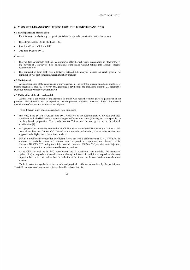
• First one, made by INSS, CRIEPI and DNV consisted of the determination of the heat exchange
coefficient with air (Hair) and the heat exchange coefficient with water (Hwater), as it was specified inthe benchmark proposition. The conduction coefficient was the one given in the benchmark specification [4].
• JNC proposed to reduce the conduction coefficient based on material data: usually K values of thismaterial are less than 20 W/m/°C. Instead of the radiation calculation, Hair at outer surface was
d t b high th H i t i f
7/31/2019 Nea Study of Thermal Fatigue
http://slidepdf.com/reader/full/nea-study-of-thermal-fatigue 26/147
NEA/CSNI/R(2005)2
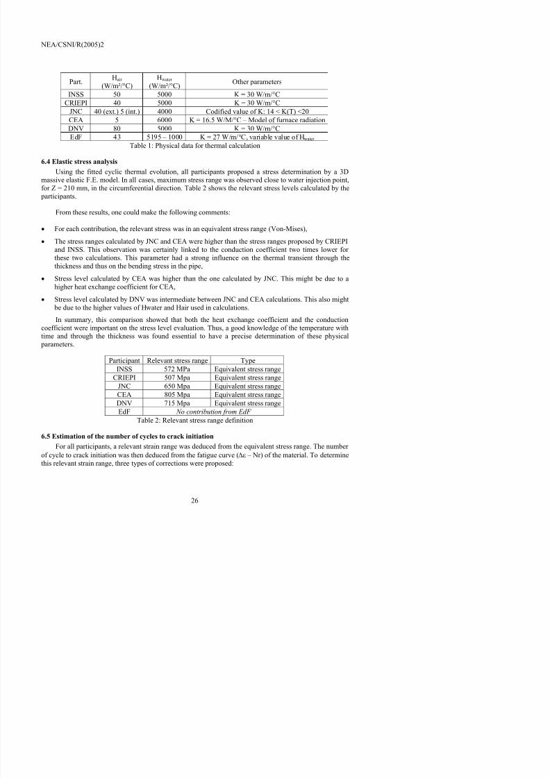
Part. Hair
(W/m²/°C)Hwater
(W/m²/°C) Other parameters
INSS 50 5000 K = 30 W/m/°CCRIEPI 40 5000 K = 30 W/m/°C
JNC 40 (ext.) 5 (int.) 4000 Codified value of K: 14 < K(T) <20CEA 5 6000 K = 16.5 W/M/°C – Model of furnace radiationDNV 80 5000 K = 30 W/m/°C
EdF 43 5195 – 1000 K = 27 W/m/°C, variable value of Hwater Table 1: Physical data for thermal calculation
6.4 Elastic stress analysisUsing the fitted cyclic thermal evolution, all participants proposed a stress determination by a 3D
massive elastic F.E. model. In all cases, maximum stress range was observed close to water injection point,for Z = 210 mm, in the circumferential direction. Table 2 shows the relevant stress levels calculated by the participants.
From these results, one could make the following comments:
• For each contribution, the relevant stress was in an equivalent stress range (Von-Mises),• The stress ranges calculated by JNC and CEA were higher than the stress ranges proposed by CRIEPI
and INSS. This observation was certainly linked to the conduction coefficient two times lower for these two calculations. This parameter had a strong influence on the thermal transient through thethickness and thus on the bending stress in the pipe,
• Stress level calculated by CEA was higher than the one calculated by JNC. This might be due to ahigher heat exchange coefficient for CEA,
• Stress level calculated by DNV was intermediate between JNC and CEA calculations. This also might be due to the higher values of Hwater and Hair used in calculations.In summary, this comparison showed that both the heat exchange coefficient and the conduction
coefficient were important on the stress level evaluation. Thus, a good knowledge of the temperature withtime and through the thickness was found essential to have a precise determination of these physical parameters.
Participant Relevant stress range TypeINSS 572 MPa Equivalent stress range
CRIEPI 507 Mpa Equivalent stress rangeJNC 650 Mpa Equivalent stress range
7/31/2019 Nea Study of Thermal Fatigue
http://slidepdf.com/reader/full/nea-study-of-thermal-fatigue 27/147
NEA/CSNI/R(2005)2
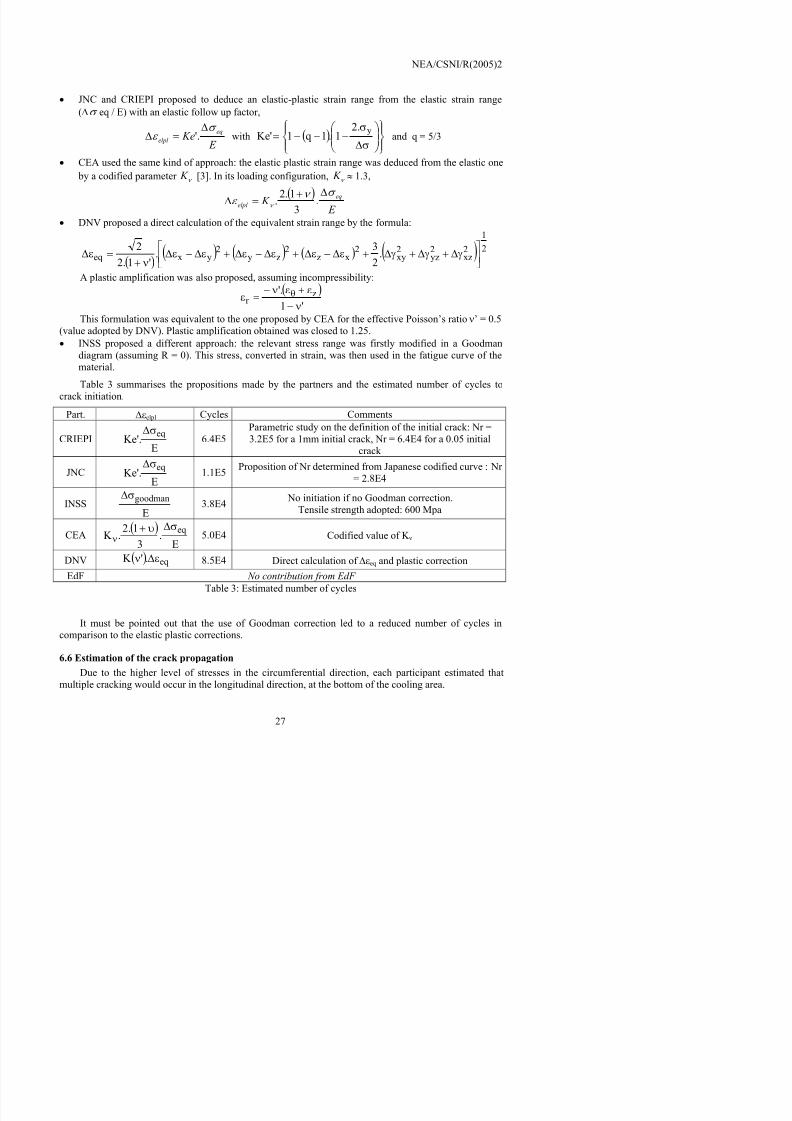
•
JNC and CRIEPI proposed to deduce an elastic-plastic strain range from the elastic strain range(∆σ eq / E) with an elastic follow up factor,
E Ke eq
elpl
σ
ε ∆
=∆ '. with ( )
σ∆σ
−−−= y.21.1q1'Ke and q = 5/3
• CEA used the same kind of approach: the elastic plastic strain range was deduced from the elastic one by a codified parameter ν K [3]. In its loading configuration,ν K ≈ 1.3,
( ) E K
eqelpl
σ ν
ε ν
∆+=∆ .3
1.2.
• DNV proposed a direct calculation of the equivalent strain range by the formula:
( ) ( ) ( ) ( ) ( )21
2xz
2yz
2xy
2xz
2zy
2yxeq .
23.
'1.22 γ∆+γ∆+γ∆+ε∆−ε∆+ε∆−ε∆+ε∆−ε∆
ν+=ε∆
A plastic amplification was also proposed, assuming incompressibility:( )
'1'. z
r ν−ε+εν−
=εθ
This formulation was equivalent to the one proposed by CEA for the effective Poisson’s ratioν’ = 0.5
(value adopted by DNV). Plastic amplification obtained was closed to 1.25.• INSS proposed a different approach: the relevant stress range was firstly modified in a Goodman
diagram (assuming R = 0). This stress, converted in strain, was then used in the fatigue curve of thematerial.Table 3 summarises the propositions made by the partners and the estimated number of cycles to
crack initiation.Part. ∆εelpl Cycles Comments
CRIEPIE
'.Ke eqσ∆ 6.4E5
Parametric study on the definition of the initial crack: Nr =3.2E5 for a 1mm initial crack, Nr = 6.4E4 for a 0.05 initial
crack
JNCE
'.Ke eqσ∆ 1.1E5 Proposition of Nr determined from Japanese codified curve : Nr
= 2.8E4
INSSE
goodmanσ∆ 3.8E4 No initiation if no Goodman correction.Tensile strength adopted: 600 Mpa
CEA ( )E
.3
1.2.K eqσ∆υ+ν 5.0E4 Codified value of K ν
( )'K ∆
7/31/2019 Nea Study of Thermal Fatigue
http://slidepdf.com/reader/full/nea-study-of-thermal-fatigue 28/147
NEA/CSNI/R(2005)2
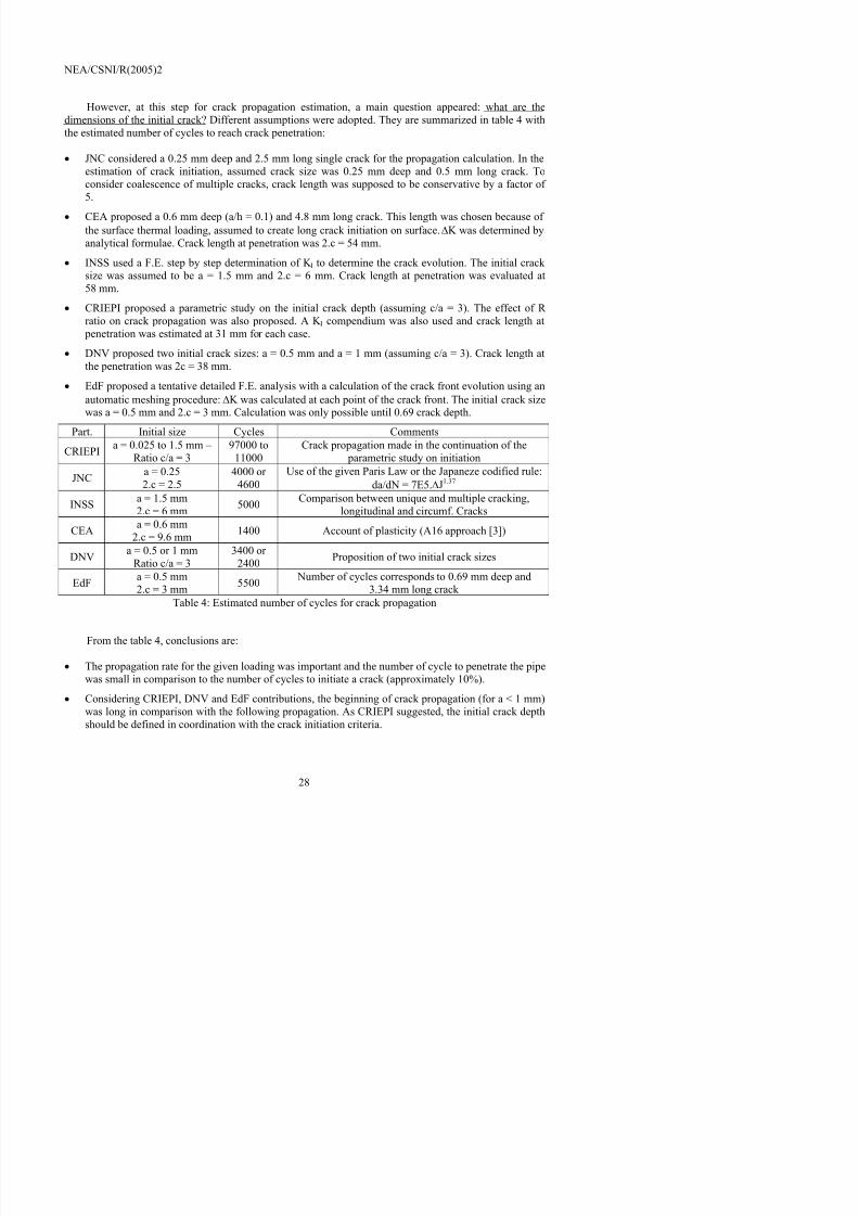
However, at this step for crack propagation estimation, a main question appeared: what are thedimensions of the initial crack? Different assumptions were adopted. They are summarized in table 4 withthe estimated number of cycles to reach crack penetration:
• JNC considered a 0.25 mm deep and 2.5 mm long single crack for the propagation calculation. In theestimation of crack initiation, assumed crack size was 0.25 mm deep and 0.5 mm long crack. Toconsider coalescence of multiple cracks, crack length was supposed to be conservative by a factor of 5.
• CEA proposed a 0.6 mm deep (a/h = 0.1) and 4.8 mm long crack. This length was chosen because of the surface thermal loading, assumed to create long crack initiation on surface.∆K was determined byanalytical formulae. Crack length at penetration was 2.c = 54 mm.
• INSS used a F.E. step by step determination of K I to determine the crack evolution. The initial crack size was assumed to be a = 1.5 mm and 2.c = 6 mm. Crack length at penetration was evaluated at58 mm.
• CRIEPI proposed a parametric study on the initial crack depth (assuming c/a = 3). The effect of R
ratio on crack propagation was also proposed. A K I compendium was also used and crack length at penetration was estimated at 31 mm for each case.• DNV proposed two initial crack sizes: a = 0.5 mm and a = 1 mm (assuming c/a = 3). Crack length at
the penetration was 2c = 38 mm.• EdF proposed a tentative detailed F.E. analysis with a calculation of the crack front evolution using an
automatic meshing procedure:∆K was calculated at each point of the crack front. The initial crack sizewas a = 0.5 mm and 2.c = 3 mm. Calculation was only possible until 0.69 crack depth.
Part. Initial size Cycles CommentsCRIEPI a = 0.025 to 1.5 mm –
Ratio c/a = 397000 to11000
Crack propagation made in the continuation of the parametric study on initiation
JNC a = 0.252.c = 2.5
4000 or 4600
Use of the given Paris Law or the Japaneze codified rule:da/dN = 7E5.∆J1.37
INSS a = 1.5 mm2.c = 6 mm 5000 Comparison between unique and multiple cracking,
longitudinal and circumf. Cracks
CEAa = 0.6 mm
2.c = 9.6 mm 1400 Account of plasticity (A16 approach [3])DNV a = 0.5 or 1 mm
Ratio c/a = 33400 or 2400 Proposition of two initial crack sizes
EdF a = 0.5 mm2.c = 3 mm 5500 Number of cycles corresponds to 0.69 mm deep and
3.34 mm long crack Table 4: Estimated number of cycles for crack propagation
7/31/2019 Nea Study of Thermal Fatigue
http://slidepdf.com/reader/full/nea-study-of-thermal-fatigue 29/147
NEA/CSNI/R(2005)2
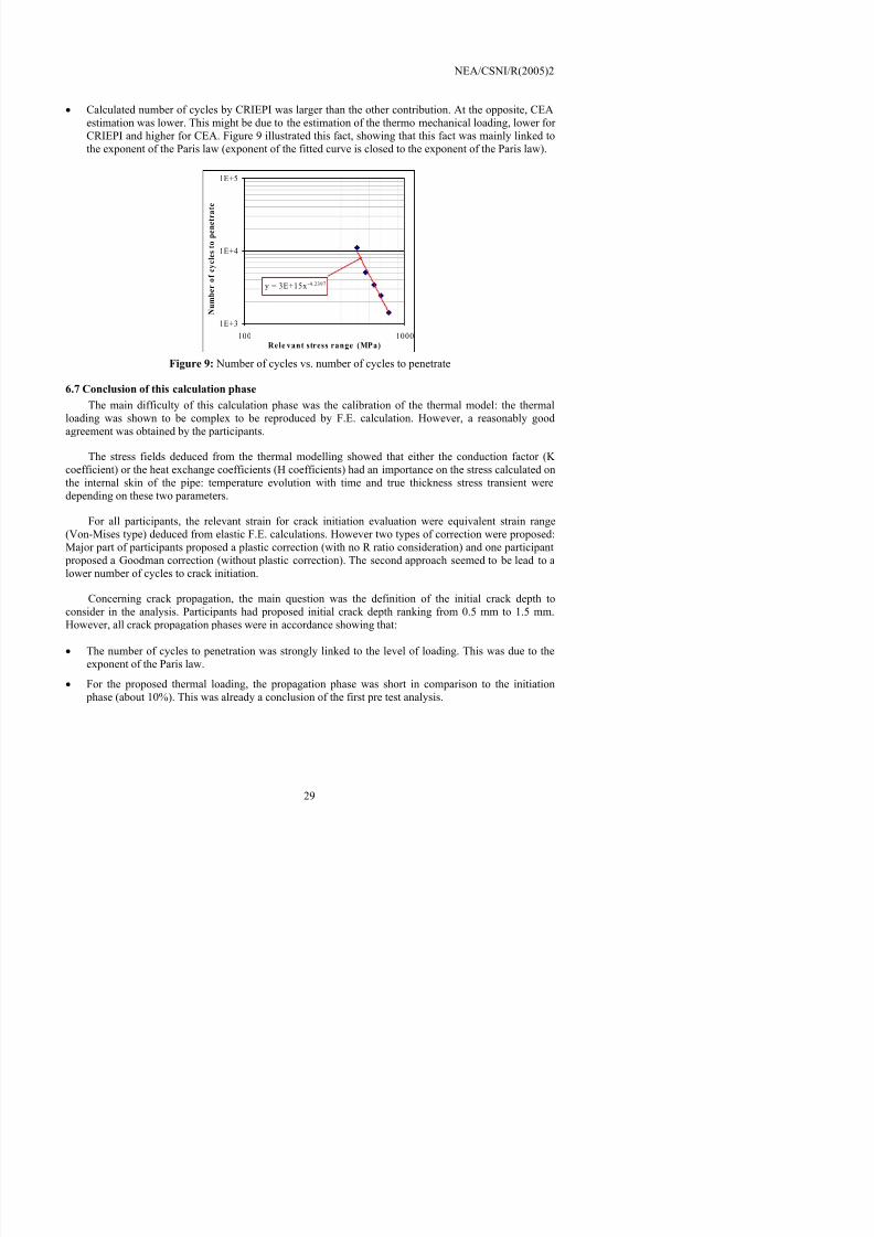
•
Calculated number of cycles by CRIEPI was larger than the other contribution. At the opposite, CEAestimation was lower. This might be due to the estimation of the thermo mechanical loading, lower for CRIEPI and higher for CEA. Figure 9 illustrated this fact, showing that this fact was mainly linked tothe exponent of the Paris law (exponent of the fitted curve is closed to the exponent of the Paris law).
y = 3E+15x -4.2397
1E+3
1E+4
1E+5
100 1000Rele vant stress range (MPa)
N u m
b e r o
f c y c l e s
t o p e n e
t r a t e
Figure 9: Number of cycles vs. number of cycles to penetrate
6.7 Conclusion of this calculation phaseThe main difficulty of this calculation phase was the calibration of the thermal model: the thermal
loading was shown to be complex to be reproduced by F.E. calculation. However, a reasonably goodagreement was obtained by the participants.
The stress fields deduced from the thermal modelling showed that either the conduction factor (K coefficient) or the heat exchange coefficients (H coefficients) had an importance on the stress calculated onthe internal skin of the pipe: temperature evolution with time and true thickness stress transient weredepending on these two parameters.
For all participants, the relevant strain for crack initiation evaluation were equivalent strain range(Von-Mises type) deduced from elastic F.E. calculations. However two types of correction were proposed:Major part of participants proposed a plastic correction (with no R ratio consideration) and one participant proposed a Goodman correction (without plastic correction). The second approach seemed to be lead to alower number of cycles to crack initiation.
Concerning crack propagation, the main question was the definition of the initial crack depth toconsider in the analysis Participants had proposed initial crack depth ranking from 0 5 mm to 1 5 mm
7/31/2019 Nea Study of Thermal Fatigue
http://slidepdf.com/reader/full/nea-study-of-thermal-fatigue 30/147
NEA/CSNI/R(2005)2
7. TEST OBSERVATION
The test in support of the benchmark was conducted in parallel of the blind analyses. The objectivewas to compare, in fine, the participant predictions to the experimental results.
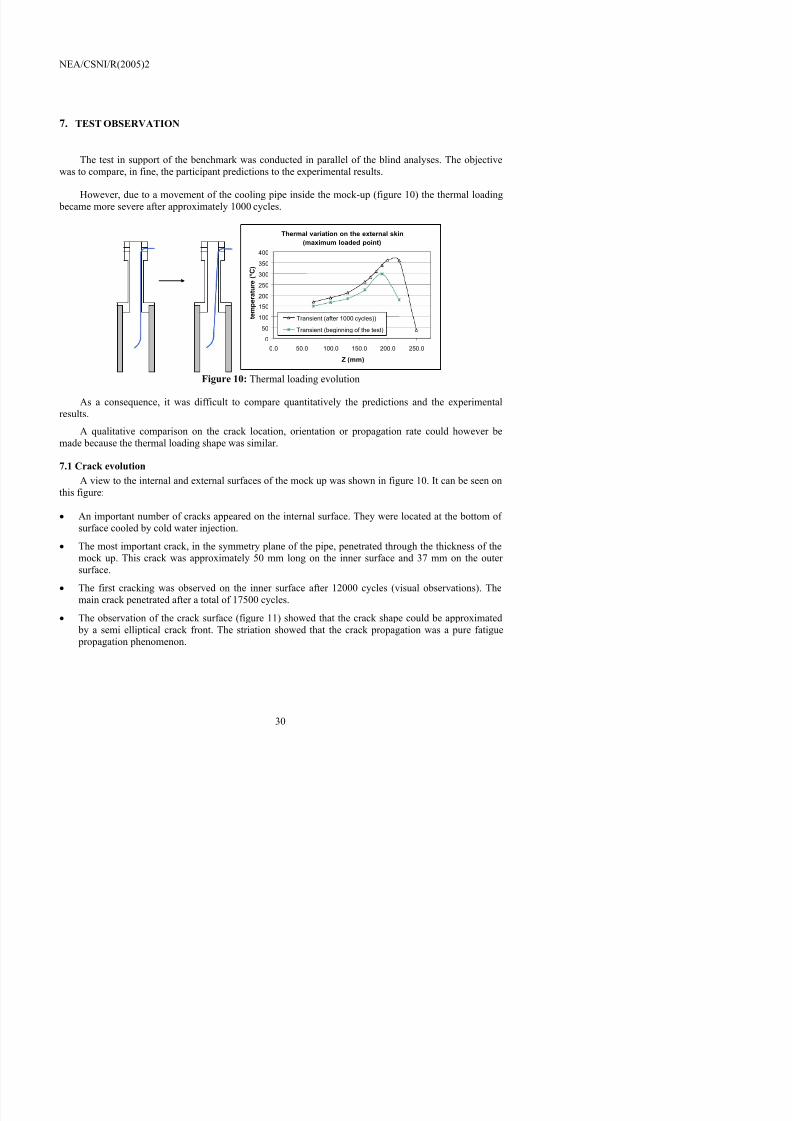
However, due to a movement of the cooling pipe inside the mock-up (figure 10) the thermal loading became more severe after approximately 1000 cycles.
Thermal variation on the external skin (maximum loaded point)
0
50
100
150200
250
300
350
400
0.0 50.0 100.0 150.0 200.0 250.0
Z (mm)
t e m p e r a
t u r e
( ° C )
Transient (after 1000 cycles))
Transient (beginning of the test)
Figure 10: Thermal loading evolution
As a consequence, it was difficult to compare quantitatively the predictions and the experimentalresults.
A qualitative comparison on the crack location, orientation or propagation rate could however bemade because the thermal loading shape was similar.
7.1 Crack evolutionA view to the internal and external surfaces of the mock up was shown in figure 10. It can be seen on
this figure:• An important number of cracks appeared on the internal surface. They were located at the bottom of
surface cooled by cold water injection.• The most important crack, in the symmetry plane of the pipe, penetrated through the thickness of the
k Thi k i t l 50 l th i f d 37 th t
7/31/2019 Nea Study of Thermal Fatigue
http://slidepdf.com/reader/full/nea-study-of-thermal-fatigue 31/147
NEA/CSNI/R(2005)2
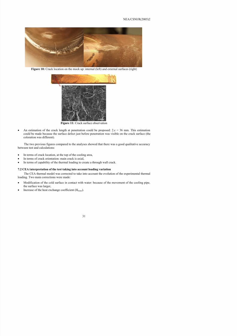
Figure 10: Crack location on the mock up: internal (left) and external surfaces (right)
Figure 11: Crack surface observation
• An estimation of the crack length at penetration could be proposed: 2.c = 36 mm. This estimationcould be made because the surface defect just before penetration was visible on the crack surface (thecoloration was different).
The two previous figures compared to the analyses showed that there was a good qualitative accuracy
between test and calculations:• In terms of crack location, at the top of the cooling area,• In terms of crack orientation: main crack is axial,• In terms of capability of the thermal loading to create a through wall crack.
7/31/2019 Nea Study of Thermal Fatigue
http://slidepdf.com/reader/full/nea-study-of-thermal-fatigue 32/147
7/31/2019 Nea Study of Thermal Fatigue
http://slidepdf.com/reader/full/nea-study-of-thermal-fatigue 33/147
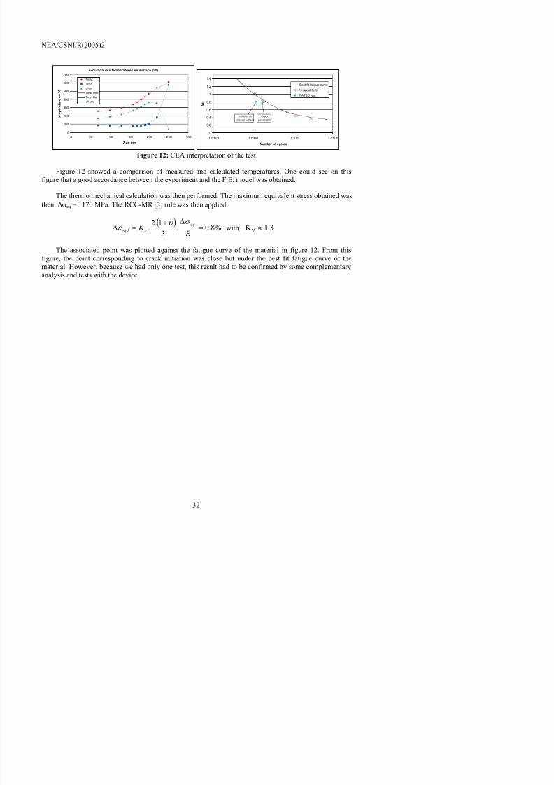
NEA/CSNI/R(2005)2
8. DISCUSSION OF THE RESULTS – RECOMMENDATIONS
The experimental configuration and the associated F.E. interpretation proposed in this benchmark were relatively simple but had led to interesting results in terms of integrity assessment evaluation under thermal loading.
Concerning thermal loading evaluation, the different calculations performed showed the importanceof the physical parameter such as K (conduction coefficient) and H (heat exchange coefficient) on thetemperature and stress variation evaluation: first term had a major effect on the stress transient through thethickness although the second one had an importance on the local stress variation on surface.
More generally, for a given thermal loading, it was difficult to reproduce the measured temperatures by the numerical simulation.
Concerning relevant stress and strain evaluation for crack initiation, all contributors proposed anequivalent stress and strain ranges (Von-Mises type). But two corrections were proposed to amplify theelastic strain range determined from thermo mechanical F.E. calculation: a plastic correction to take intoaccount the plasticity which might occur on the surface (due to high level of loading) or a Goodmancorrection, to take into account a R ratio.
From the proposed results, the Goodman correction seems to be more severe (in terms of calculatednumber of cycles to crack initiation).
From these estimates, the location and the orientation of the crack initiation were correctly found: asin the test, the major cracking was predicted at the top cooling area, in the axial direction. Thus, even if therelevant strain was an equivalent strain range, the major crack orientation was governed by the maximum principal stress range (circumferential stress in the symmetry plane).
Concerning crack propagation phase, multiple cracking was observed, but only one of them emergedfrom the crack network and penetrated the thickness of the pipe.
From the analysis side, the main difficulty was the definition of the initial crack size. This choice hadan importance on the integrity assessment evaluation:
• Crack propagation at the beginning was important in terms of number of cycles to propagate (becauseof the low values of ∆K for small cracks).
7/31/2019 Nea Study of Thermal Fatigue
http://slidepdf.com/reader/full/nea-study-of-thermal-fatigue 34/147
NEA/CSNI/R(2005)2
9. CONCLUSIONS OF THE BENCHMARK
The benchmark proposed in the frame of the OECD/NEA/CSNI/IAGE working group was nowcompleted. Organised in three major steps, it allowed defining, realising and analysing an example of fatigue crack propagation under pure thermal loading in which important cracking, up to penetration, wasobserved.
• First step devoted to pre calculation gave the first main conclusions on the minimum thermal loadingto observe cracking with the mock up, the specimen geometry or the models needed to have a goodrepresentation of the loading,
• Second step was an experimental qualification of the thermal loading. The temperature measurementsmade on a special mock-up were sent to participants to have a good representation of the thermalloading for analyses,
•
Final step was the blind interpretation of the test. At this step, participants were asked to estimate thenumber of cycles to crack initiation and to full propagation through the thickness. The test was performed in parallel.Due to a movement of the cooling pipe at the beginning of the test, the thermal loading was more
severe than the loading characterised with the thermal mock-up. It was difficult to compare quantitativelythe prediction of the participants with the experiment.
However, a qualitative comparison showed that predictions were in good agreement with the testresults:• The location and the orientation of the cracks were predicted by the participants: due to the
circumferential stresses, axial cracks are dominant, at the bottom of the cooling area.• The capability of the cracks to propagate through the thickness was predicted and, for all participants,
the number of cycles to penetrate the pipe wall was small compared to the number of cycles for initiation. This was observed during the test with 12000 cycles to initiate a crack and 17500 for thecomplete penetration.
CEA post interpretation made with corrected thermal loading showed that the point corresponding tocrack initiation was below the fatigue best fit curve of the material. This first result had to be confirmedwith complementary tests and analyses.

7/31/2019 Nea Study of Thermal Fatigue
http://slidepdf.com/reader/full/nea-study-of-thermal-fatigue 35/147
NEA/CSNI/R(2005)2
Appendix I: Thermal loading characterization
7/31/2019 Nea Study of Thermal Fatigue
http://slidepdf.com/reader/full/nea-study-of-thermal-fatigue 36/147
NEA/CSNI/R(2005)2
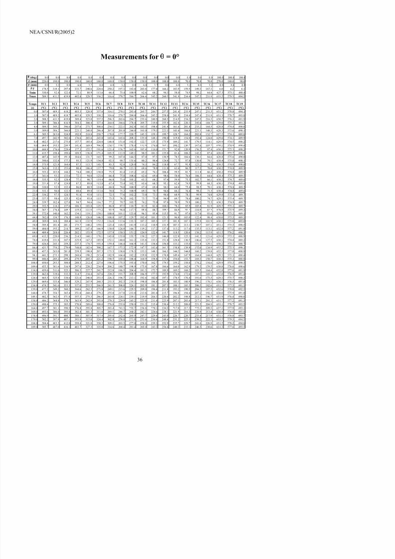
Measurements for = 0°
(deg.) 0.0 0.0 0.0 0.0 0.0 0.0 0.0 0.0 0.0 0.0 0.0 0.0 0.0 0.0 0.0 0.0 180.0 180.0 180.0Z (mm) 220.0 190.0 190.0 190.0 160.0 160.0 160.0 130.0 130.0 130.0 100.0 100.0 100.0 70.0 70.0 70.0 270.0 180.0 90.0
(mm) 0.0 3.2 0.0 6.0 3.2 0.0 6.0 3.2 0.0 6.0 3.2 0.0 6.0 3.2 0.0 3.2 0.0 0.0 0.0T 178.5 319.1 297.4 333.7 240.6 224.6 250.2 197.3 183.8 203.8 177.0 166.2 183.9 159.5 149.3 167.3 6.0 6.2 6.1
Tmin 330.8 92.4 122.4 72.1 88.9 113.6 66.4 73.4 100.9 62.6 68.2 94.3 58.0 74.9 98.2 64.6 627.5 573.1 488.4Tmax 509.3 411.5 419.8 405.8 329.5 338.2 316.6 270.7 284.7 266.4 245.2 260.5 241.9 234.4 247.5 231.9 633.5 579.3 494.5
Temps TC1 TC2 TC3 TC4 TC5 TC6 TC7 TC8 TC9 TC10 TC11 TC12 TC13 TC14 TC15 TC16 TC17 TC18 TC19(s) (°C) (°C) (°C) (°C) (°C) (°C) (°C) (°C) (°C) (°C) (°C) (°C) (°C) (°C) (°C) (°C) (°C) (°C) (°C)
0.0 507.6 409.1 418.2 405.3 328.8 337.6 316.1 270.1 283.4 265.7 244.7 257.5 241.4 233.9 247.1 231.5 631.2 578.8 494.11.0 507.9 409.2 418.7 405.8 329.5 338.2 316.6 270.7 284.0 266.4 245.2 258.0 241.9 234.4 247.4 231.9 631.3 578.7 493.82.0 508.3 411.5 419.8 389.4 323.0 337.5 296.3 265.6 284.7 235.6 240.9 260.5 214.9 234.2 247.5 216.3 630.7 576.1 491.93.0 509.1 386.4 416.9 304.3 300.4 327.4 264.0 244.6 278.4 205.7 219.8 255.9 182.4 220.3 245.0 184.7 629.0 575.2 491.34.0 509.3 345.2 396.6 257.6 273.7 308.6 234.1 222.1 262.8 183.5 198.4 241.4 161.6 201.8 235.2 164.5 628.8 574.4 490.85.0 509.0 306.2 366.0 225.1 248.0 286.4 207.8 201.0 244.0 165.0 179.5 223.5 145.4 184.0 221.1 148.5 628.3 573.6 490.16.1 505.5 263.0 324.9 192.9 218.8 258.7 178.0 177.7 220.7 145.3 159.1 199.7 128.7 164.2 202.8 132.7 627.5 574.1 489.87.0 497.7 242.9 302.6 176.6 203.6 243.0 165.6 165.6 208.1 135.0 148.1 190.0 119.8 154.0 192.4 124.0 629.6 574.1 489.98.0 482.5 217.6 275.0 157.7 185.4 224.0 148.8 151.0 192.5 122.7 135.3 175.9 109.2 141.7 179.5 114.1 629.9 574.5 490.29.0 464.8 195.5 250.5 141.4 169.4 206.9 134.1 138.2 178.4 111.9 124.0 163.1 100.2 130.7 167.6 105.2 630.1 574.9 490.4
10.0 444.8 176.6 228.6 127.3 155.2 191.6 121.4 126.7 165.6 102.4 114.0 151.7 92.0 120.9 156.5 97.4 630.3 575.3 490.311.0 415.7 150.4 199.6 109.5 136.8 171.4 103.5 111.9 149.1 90.5 101.2 135.0 81.6 108.2 142.2 87.4 628.8 575.7 490.112.0 407.4 143.9 191.8 104.6 131.7 165.7 99.2 107.8 144.5 87.0 97.5 130.9 78.5 104.6 138.1 84.6 628.8 575.6 490.013.0 390.6 132.8 177.3 95.3 121.9 154.8 92.5 99.7 135.6 80.2 90.4 124.8 72.7 97.8 130.0 79.1 630.4 575.0 490.114.0 375.9 121.8 164.6 87.3 113.7 145.7 85.3 92.8 128.0 74.5 84.2 118.0 67.7 91.8 123.2 74.2 630.3 574.8 490.015.0 363.6 112.2 153.6 80.4 106.4 137.7 79.0 86.7 121.3 69.6 78.8 111.8 63.4 86.5 117.2 70.0 630.2 574.8 489.916.0 353.2 103.8 144.2 74.4 100.2 130.8 73.5 81.4 115.2 65.2 74.1 106.4 59.5 81.7 111.8 66.2 630.2 574.8 489.917.1 341.6 93.2 133.6 72.1 94.0 123.6 66.4 75.8 108.6 62.6 69.4 98.6 58.0 76.6 106.3 64.6 628.4 575.2 489.518.0 335.5 92.5 128.4 77.1 90.7 119.4 66.8 73.8 105.2 63.3 68.2 97.4 59.9 75.3 102.7 66.1 630.2 574.7 489.619.0 331.4 92.4 124.0 82.3 89.0 115.8 67.4 73.4 102.2 65.6 68.5 95.1 62.4 74.9 99.9 68.3 630.1 574.8 489.620.0 330.8 93.9 122.4 86.0 88.9 114.0 68.8 74.0 100.9 67.4 69.4 94.3 64.4 75.4 98.5 70.1 630.3 574.8 489.521.0 332.1 96.0 122.5 88.6 89.8 113.6 70.8 75.2 100.9 69.3 70.7 94.6 66.2 76.4 98.2 71.5 630.4 574.8 489.622.0 336.2 97.5 124.5 91.6 93.0 115.1 72.5 77.6 102.2 73.0 73.1 94.4 68.9 78.1 99.9 74.0 629.0 575.4 489.7
23.0 337.5 98.6 125.3 92.6 93.8 115.7 73.5 78.3 102.7 73.7 73.8 94.9 69.7 78.6 100.2 74.7 629.1 575.4 489.724.0 339.7 102.4 127.0 94.7 94.6 116.7 77.2 79.7 103.7 74.2 75.0 97.8 70.9 79.9 100.2 75.5 630.3 574.9 489.729.0 352.5 114.2 137.6 106.3 103.8 125.5 86.8 87.5 110.7 81.9 82.4 104.3 78.2 85.9 105.8 81.9 629.5 575.1 489.734.0 363.7 126.4 149.7 119.5 111.6 133.2 93.9 94.8 117.3 88.8 88.7 109.7 84.9 91.7 110.9 87.5 628.9 575.9 489.339.1 372.8 140.0 162.2 134.1 119.1 139.1 100.8 101.1 123.8 96.3 95.4 115.5 91.7 97.6 117.0 93.6 629.4 573.2 489.144.0 382.0 154.7 176.3 148.9 126.8 146.5 108.8 107.2 129.7 102.4 101.1 121.5 96.8 103.0 122.4 98.4 630.0 573.5 489.349.0 389.0 168.3 188.4 161.9 132.9 152.2 116.8 112.6 135.3 107.2 105.5 127.1 101.9 107.3 125.9 101.9 630.1 575.8 489.054.0 395.4 181.4 201.1 175.7 140.2 159.1 123.4 118.5 141.9 113.2 110.9 131.9 107.3 113.1 130.7 107.1 631.1 575.3 490.559.0 404.0 195.2 214.7 189.2 147.4 166.9 130.8 124.8 146.7 119.2 117.2 137.4 113.2 117.4 135.5 113.1 632.8 577.2 491.064.0 409.4 208.0 226.4 202.1 153.9 172.5 137.9 130.3 151.2 124.9 122.4 141.7 118.5 120.6 138.2 115.9 631.5 576.2 490.369.0 413.5 220.0 236.2 214.5 160.1 178.1 145.0 135.0 155.7 130.2 127.5 146.0 122.8 125.3 141.3 121.6 629.8 573.1 488.974.0 419.8 231.8 247.5 225.9 167.2 185.9 152.1 140.8 161.2 135.8 133.3 151.0 128.0 130.5 146.6 127.5 630.1 574.4 489.279.0 426.8 243.1 259.2 237.3 174.7 193.4 159.4 146.4 166.9 141.5 138.6 156.0 133.2 135.0 151.8 129.1 630.2 575.2 488.7
84.0 431.5 254.2 270.0 248.0 182.6 200.2 167.2 152.3 172.9 147.5 143.4 161.3 138.8 138.8 155.0 134.9 632.2 575.3 490.189.0 437.5 265.0 281.0 259.3 190.8 207.3 175.3 158.8 178.5 153.5 148.1 166.5 144.3 144.0 160.2 139.8 632.5 577.0 490.994.1 441.3 275.1 290.1 268.6 198.2 213.4 182.9 164.4 182.2 159.8 152.9 170.8 149.4 147.9 164.8 144.8 629.3 575.1 488.499.0 446.8 285.2 299.2 279.5 205.3 221.2 190.5 169.4 188.4 164.9 158.8 175.6 154.0 153.7 169.3 150.7 630.3 575.1 488.8
104.0 450.6 293.3 308.0 288.3 212.4 227.6 196.6 175.5 193.4 170.0 162.7 179.5 159.2 158.0 174.2 154.6 629.9 575.3 490.3109.0 455.3 301.6 316.9 297.0 220.2 234.9 204.2 180.7 198.9 175.8 167.8 184.6 164.0 162.9 179.5 159.5 630.8 576.6 490.6114.0 459.6 311.6 325.1 306.3 227.7 241.7 212.8 186.5 204.4 181.3 172.7 189.9 169.2 168.2 183.5 164.4 632.8 577.6 491.9119.0 462.8 319.6 332.2 314.7 234.4 247.6 220.2 191.7 208.9 186.9 177.5 193.9 174.0 172.6 187.2 169.1 632.0 576.9 491.4124 0 465 5 325 8 338 6 321 6 240 8 253 5 226 3 196 7 213 1 192 4 182 0 197 1 178 5 176 4 191 6 173 5 629 3 575 7 490 3
7/31/2019 Nea Study of Thermal Fatigue
http://slidepdf.com/reader/full/nea-study-of-thermal-fatigue 37/147
NEA/CSNI/R(2005)2
Measurements for θ = 20°
(deg.) 20.0 20.0 20.0 20.0 20.0 20.0 20.0 20.0 20.0 20.0 20.0 20.0 20.0 20.0 20.0 20.0 200.0 200.0 200.0Z (mm) 220.0 190.0 190.0 190.0 160.0 160.0 160.0 130.0 130.0 130.0 100.0 100.0 100.0 70.0 70.0 70.0 270.0 180.0 90.0
(mm) 0.0 3.2 0.0 6.0 3.2 0.0 6.0 3.2 0.0 6.0 3.2 0.0 6.0 3.2 0.0 3.2 0.0 0.0 0.0T 152.7 326.2 303.9 342.6 246.7 230.6 257.7 208.6 194.4 215.4 187.1 175.3 193.4 167.1 155.0 175.0 8.4 6.8 7.4
Tmin 367.1 96.8 128.1 77.7 96.5 121.1 75.9 75.4 102.2 65.1 70.9 96.6 61.8 80.4 104.4 69.5 635.0 579.4 493.5Tmax 519.8 423.0 432.0 420.3 343.2 351.7 333.6 284.0 296.6 280.5 258.0 271.9 255.2 247.5 259.4 244.5 643.4 586.2 500.9
Temps TC1 TC2 TC3 TC4 TC5 TC6 TC7 TC8 TC9 TC10 TC11 TC12 TC13 TC14 TC15 TC16 TC17 TC18 TC19(s) (°C) (°C) (°C) (°C) (°C) (°C) (°C) (°C) (°C) (°C) (°C) (°C) (°C) (°C) (°C) (°C) (°C) (°C) (°C)
0.0 519.3 422.0 431.0 420.3 342.3 350.6 333.6 283.0 295.6 280.5 257.1 271.4 255.2 246.8 259.4 244.0 640.7 585.6 500.91.0 519.8 423.0 432.0 420.3 343.2 351.7 333.2 284.0 296.6 273.1 258.0 271.9 252.5 247.5 259.1 244.5 638.1 583.7 499.32.1 519.4 408.3 431.1 340.0 324.2 346.6 296.7 261.1 292.2 222.6 236.0 269.2 200.0 238.0 258.6 203.6 635.6 581.9 498.03.0 518.9 378.1 420.7 293.5 304.2 335.8 272.2 243.0 281.8 202.4 219.2 259.6 181.5 223.8 252.5 186.4 635.4 582.3 496.54.0 518.9 335.9 393.6 253.4 277.8 315.7 243.2 219.8 262.9 180.8 197.4 242.0 161.5 204.9 239.7 168.2 635.4 580.0 495.85.0 518.5 298.0 360.5 222.5 252.8 293.0 217.4 198.7 242.6 162.8 178.1 222.7 145.6 187.3 224.5 153.1 635.0 579.4 495.36.0 516.4 264.8 327.5 197.3 230.1 271.0 195.0 180.1 223.4 147.0 161.3 204.9 131.8 171.7 209.5 140.2 635.5 579.8 495.37.0 504.3 223.6 282.4 167.0 200.6 240.5 166.7 155.4 198.1 127.1 140.2 181.5 113.9 152.0 189.5 123.8 636.3 580.7 495.48.0 498.6 212.2 269.7 158.8 192.3 231.7 158.8 148.6 190.8 121.5 134.3 174.9 109.0 146.4 183.4 119.2 636.4 580.6 495.59.0 485.2 190.9 246.8 142.8 175.8 214.5 143.7 137.1 175.9 110.6 122.8 161.7 101.0 134.9 170.8 110.0 636.2 581.5 495.7
10.0 469.3 172.6 226.1 128.9 161.4 198.8 130.7 125.8 163.0 101.3 112.9 150.3 93.1 124.9 159.9 102.1 636.3 581.6 495.411.0 453.2 156.8 207.5 117.0 148.8 184.7 119.2 115.9 151.8 93.2 104.2 140.4 86.1 116.3 150.3 95.0 636.3 581.4 495.212.0 437.6 143.2 191.5 106.6 137.8 172.4 109.2 107.2 142.1 86.0 96.6 131.6 79.9 108.5 141.7 88.6 636.3 581.4 495.113.1 419.1 128.4 172.7 95.8 125.8 160.0 98.5 96.2 131.8 78.3 89.1 122.4 71.9 100.2 132.1 82.6 636.7 580.0 495.514.0 409.6 120.5 165.7 90.1 119.6 152.2 92.8 92.9 125.9 74.2 83.9 117.2 70.0 95.6 127.2 78.2 636.4 581.0 494.915.0 397.3 111.4 154.9 83.3 112.1 144.1 86.1 86.6 119.2 69.4 78.7 111.5 65.5 90.2 121.1 73.7 636.5 580.1 495.016.0 386.8 103.1 145.5 77.7 105.6 136.6 80.4 81.4 113.4 65.1 73.9 106.2 61.8 85.3 115.7 69.5 636.8 580.1 495.117.0 377.7 97.4 137.4 81.7 100.3 130.1 76.4 77.4 108.1 65.3 70.9 101.4 63.1 81.7 110.7 70.4 636.9 580.2 494.918.0 370.3 96.8 128.9 90.3 96.7 124.7 75.9 75.4 103.2 69.0 72.3 97.0 66.1 80.4 105.6 75.1 636.1 580.6 493.819.0 369.3 97.5 128.1 91.9 96.5 123.4 76.4 75.8 102.6 70.0 72.7 96.6 67.1 80.6 104.9 75.6 636.0 580.6 494.020.0 367.1 99.2 128.7 94.6 97.2 121.3 78.2 77.9 102.2 72.3 72.6 96.8 70.1 81.3 104.4 76.4 636.7 579.8 495.421.0 367.9 101.3 129.5 97.1 98.5 121.1 79.9 79.3 102.7 74.5 74.3 97.4 71.8 82.3 104.7 77.8 636.7 579.9 495.422.0 368.9 103.6 131.1 99.5 99.7 121.8 81.8 80.9 103.6 76.2 75.8 98.5 73.5 83.4 105.3 79.1 636.7 579.7 495.223.0 370.3 106.0 133.0 102.1 101.3 122.8 83.7 82.5 104.8 78.0 77.3 99.7 75.1 84.5 106.1 80.3 636.7 579.7 495.224.1 372.6 109.3 134.8 105.2 102.9 125.2 85.7 83.5 106.6 79.6 80.0 101.3 76.0 86.1 106.9 82.5 636.3 580.5 493.829.0 380.7 123.4 147.7 120.1 111.3 133.1 94.2 91.8 114.4 87.6 87.7 108.7 83.7 92.1 112.5 88.5 636.4 580.5 493.534.0 386.4 136.2 160.8 133.4 117.4 138.0 100.4 99.1 120.5 93.6 92.9 115.0 90.7 97.2 117.5 92.7 637.4 580.1 494.839.0 394.0 150.9 175.0 148.5 124.5 144.6 107.2 105.1 126.4 99.7 99.3 121.1 96.6 102.3 122.9 97.7 637.0 580.1 494.644.0 400.6 165.1 188.2 163.2 132.0 151.0 114.2 110.4 131.9 106.3 104.6 126.1 101.2 106.6 127.8 102.2 636.7 581.0 493.949.0 406.6 180.0 201.8 177.9 139.0 157.4 121.7 116.2 137.9 112.3 110.1 131.7 106.8 112.1 132.5 107.5 638.2 580.2 494.854.0 413.2 194.4 215.5 191.1 145.7 164.2 130.1 122.6 143.4 117.8 115.7 138.2 112.9 117.0 137.1 112.7 637.7 582.0 493.959.0 418.5 208.7 228.2 205.1 153.2 171.6 138.4 128.4 149.4 123.7 121.5 144.6 118.3 122.7 142.4 118.1 639.4 581.7 495.164.0 424.7 221.2 240.7 218.6 161.0 179.1 146.2 134.5 156.0 130.1 126.7 149.4 123.6 127.2 146.9 122.5 638.2 582.8 494.869.0 429.2 233.5 252.4 231.0 168.8 185.9 153.5 140.4 162.0 136.2 131.6 153.9 128.8 132.4 151.5 127.1 639.7 582.3 495.274.0 435.8 245.1 264.3 241.8 176.9 194.0 162.0 147.1 166.9 142.4 137.5 159.7 135.0 136.6 156.6 132.7 639.1 583.0 494.979.1 441.1 258.0 275.6 254.5 185.3 202.1 171.5 153.1 173.2 148.7 142.0 165.9 138.3 141.4 161.7 136.1 640.7 582.8 496.084.0 446.5 269.0 286.9 266.4 194.1 210.0 179.6 159.2 180.2 155.2 146.4 169.1 144.1 145.5 164.9 140.8 640.7 583.3 496.289.0 451.8 278.2 296.1 276.0 201.3 217.8 186.8 164.9 184.9 160.6 152.2 173.3 149.6 150.0 168.9 146.2 642.2 584.9 497.594.0 454.8 287.3 305.2 285.8 207.8 224.2 194.3 171.5 189.7 165.8 157.5 177.2 155.8 154.7 172.2 151.1 639.7 583.6 496.199.0 458.8 297.1 314.0 295.4 216.3 231.7 202.7 177.2 195.3 172.4 162.9 182.9 161.0 159.9 178.0 156.1 641.0 583.0 497.5
104.0 464.4 306.0 322.7 304.0 225.5 239.2 210.5 182.6 201.0 179.5 168.2 188.0 165.8 164.7 184.2 161.2 641.8 584.3 497.2109.0 469.5 316.1 331.8 313.9 232.7 247.2 219.3 188.8 207.5 184.7 174.0 193.9 171.4 170.5 188.2 166.6 643.4 586.1 499.1114.0 472.6 324.5 339.3 322.6 239.9 253.7 227.2 194.7 212.5 190.7 179.3 198.2 176.8 175.3 192.1 171.6 642.5 585.4 498.7119.0 475.1 332.3 346.2 330.2 246.8 259.4 235.2 200.1 217.5 196.6 184.1 203.2 181.8 180.1 196.1 176.0 639.7 584.6 497.3
7/31/2019 Nea Study of Thermal Fatigue
http://slidepdf.com/reader/full/nea-study-of-thermal-fatigue 38/147
NEA/CSNI/R(2005)2
Measurements for θ = 40°
(deg.) 40.0 40.0 40.0 40.0 40.0 40.0 40.0 40.0 40.0 40.0 40.0 40.0 40.0 40.0 40.0 40.0 220.0 220.0 220.0Z (mm) 220.0 190.0 190.0 190.0 160.0 160.0 160.0 130.0 130.0 130.0 100.0 100.0 100.0 70.0 70.0 70.0 270.0 180.0 90.0
(mm) 0.0 3.2 0.0 6.0 3.2 0.0 6.0 3.2 0.0 6.0 3.2 0.0 6.0 3.2 0.0 3.2 0.0 0.0 0.0T 72.4 319.4 296.9 337.1 260.2 245.1 274.0 221.5 206.3 229.2 191.9 179.1 199.8 169.5 157.4 177.2 10.9 7.5 7.0
Tmin465.3 125.0 157.2 106.5 106.1 130.2 83.5 81.7 110.2 71.7 82.5 110.3 71.7 91.7 119.1 81.7 635.3 577.4 477.9
Tmax 537.7 444.4 454.1 443.6 366.3 375.3 357.5 303.2 316.5 300.9 274.4 289.4 271.5 261.2 276.5 258.9 646.2 584.9 484.9
Temps TC1 TC2 TC3 TC4 TC5 TC6 TC7 TC8 TC9 TC10 TC11 TC12 TC13 TC14 TC15 TC16 TC17 TC18 TC19(s) (°C) (°C) (°C) (°C) (°C) (°C) (°C) (°C) (°C) (°C) (°C) (°C) (°C) (°C) (°C) (°C) (°C) (°C) (°C)
0.0 536.6 443.7 453.1 442.8 365.9 374.1 357.4 302.5 315.4 300.9 273.9 288.6 271.5 260.7 275.7 258.9 640.8 583.0 483.21.0 536.8 444.4 454.1 440.4 366.3 375.3 357.5 303.2 316.5 299.2 274.4 289.4 270.7 261.2 276.2 258.7 637.2 580.1 480.82.0 536.4 443.0 454.1 438.0 358.1 374.1 335.5 289.8 315.7 254.7 263.0 289.0 231.0 259.5 276.5 236.8 635.3 578.8 480.13.0 534.2 402.6 443.6 321.9 317.8 351.4 282.5 249.4 294.8 208.3 227.0 272.1 190.7 232.8 268.0 193.8 636.1 577.5 480.64.0 533.7 381.7 432.4 299.4 304.1 340.8 267.2 237.1 284.7 197.1 216.6 263.6 181.2 223.6 262.1 185.4 636.2 577.4 480.45.0 533.4 341.0 402.0 263.4 276.9 317.6 238.3 213.6 261.7 176.9 197.8 245.1 164.3 204.6 247.9 171.3 636.2 577.8 478.56.0 532.3 305.5 368.4 236.2 251.9 293.9 213.5 192.9 240.2 159.6 180.3 227.0 149.7 188.7 232.7 158.0 637.1 578.3 478.57.0 532.2 275.0 336.5 212.8 229.7 271.6 192.0 175.0 221.1 144.8 165.0 210.5 137.0 174.3 218.3 146.2 637.7 578.8 478.98.0 532.3 248.5 307.9 192.9 210.0 251.3 173.2 159.4 203.9 131.9 151.5 195.6 125.7 161.6 205.1 135.6 638.0 579.1 479.09.1 531.1 220.1 276.1 172.7 188.0 227.4 153.3 142.4 186.3 117.3 135.5 179.0 113.5 148.8 189.3 122.9 638.1 579.0 481.0
10.0 528.9 205.6 260.0 160.4 176.8 216.0 142.8 133.6 175.0 110.4 128.9 170.0 107.0 140.0 180.9 117.7 638.6 579.6 479.311.0 526.2 188.5 240.2 148.2 162.9 200.6 130.2 123.1 163.0 101.8 119.6 159.2 99.5 130.8 170.4 110.1 638.8 579.7 479.512.0 522.8 173.8 223.1 137.3 150.8 187.1 119.5 113.8 152.4 94.2 111.4 149.7 92.6 122.6 161.2 103.2 639.0 579.7 479.413.0 518.9 161.2 208.4 128.7 140.3 175.3 109.9 105.6 143.3 87.5 103.9 141.4 86.4 115.3 152.9 97.0 638.9 579.5 479.314.0 512.2 145.5 189.6 118.1 126.2 159.1 97.8 95.0 132.7 78.3 93.1 130.5 78.3 106.6 141.9 87.7 638.8 578.7 480.715.0 509.8 141.0 184.6 114.7 122.4 155.0 94.4 92.0 129.3 75.9 90.3 127.3 76.0 103.8 138.7 85.4 638.7 578.7 480.616.0 504.3 132.4 175.1 106.5 115.5 148.2 87.7 86.5 121.6 71.7 86.1 121.1 71.7 96.9 132.8 81.7 638.3 579.0 478.717.0 499.2 126.3 166.6 111.3 109.9 141.2 83.7 82.6 116.1 72.6 82.9 115.8 73.6 92.9 127.3 83.1 638.2 578.8 478.418.0 494.2 125.0 160.6 116.8 107.0 135.9 83.5 81.7 112.1 75.1 82.5 112.1 76.4 91.7 123.0 85.4 638.0 578.7 478.319.0 489.6 126.1 157.8 121.4 106.1 132.8 84.6 82.2 110.2 77.4 83.3 110.4 78.4 91.8 120.4 87.2 637.8 578.5 478.320.1 484.6 129.2 157.2 128.1 106.5 130.2 87.2 83.9 111.4 79.7 83.7 110.3 80.6 94.0 119.1 88.0 638.1 577.9 480.1
21.0 481.8 131.4 158.6 129.8 107.7 131.3 88.5 85.1 110.6 81.6 85.6 110.6 81.9 93.3 119.2 89.8 637.8 578.4 478.122.0 478.9 135.0 161.0 134.0 109.3 132.1 90.6 86.8 111.7 83.6 87.1 111.5 83.5 94.3 119.5 90.9 637.7 578.3 478.123.0 476.5 138.7 164.0 138.1 111.1 133.4 92.6 88.7 113.2 85.4 88.5 112.7 85.0 95.3 120.2 92.0 637.7 578.3 478.024.0 474.4 142.6 167.2 142.4 112.9 134.9 94.4 90.4 114.8 87.1 89.9 114.0 86.4 96.4 121.0 93.0 637.5 578.1 477.929.0 468.1 162.7 185.7 163.3 120.8 142.2 102.2 98.7 122.5 94.7 96.7 120.5 93.0 101.4 125.6 97.8 638.0 578.4 477.934.0 466.2 181.8 204.0 183.0 127.9 149.1 110.2 105.0 128.8 100.7 102.4 126.0 98.3 106.1 129.8 102.9 638.1 578.4 477.939.0 465.6 199.7 221.1 201.1 135.6 156.7 118.4 111.4 135.0 107.0 108.4 131.4 104.3 111.5 134.5 108.4 638.4 578.5 478.944.0 465.3 216.1 236.2 217.4 143.6 164.2 127.2 117.6 141.1 113.4 114.3 137.4 110.1 116.8 139.6 113.7 639.1 577.9 479.049.0 466.8 231.1 250.7 232.2 152.0 172.2 136.1 124.0 147.3 119.8 120.1 143.2 115.8 122.2 145.0 119.0 639.3 577.8 479.354.0 468.7 244.8 263.9 245.7 160.6 179.7 145.1 130.3 153.4 126.3 125.5 148.9 121.7 127.5 150.0 123.8 639.7 577.7 479.559.0 471.3 258.0 277.2 258.7 170.0 187.6 155.1 137.2 159.9 133.3 130.8 155.2 127.8 133.3 155.8 128.7 639.1 579.6 479.464.1 474.0 270.6 289.3 271.1 179.3 196.3 164.9 144.0 166.5 140.2 136.7 161.2 134.0 138.9 161.3 134.1 639.5 579.9 479.769.0 476.1 282.0 300.3 282.9 188.9 205.1 174.0 150.6 173.3 147.1 142.5 166.5 139.9 144.6 166.7 139.4 640.8 579.3 480.2
74.0 480.3 291.3 309.6 291.8 196.5 214.7 182.1 156.5 178.4 152.6 149.2 171.1 145.2 148.8 170.9 145.6 640.4 580.1 479.779.0 482.4 301.4 319.4 301.6 205.8 223.0 191.4 163.1 184.7 159.6 154.8 176.7 151.0 153.9 176.4 150.8 640.6 580.4 479.784.0 485.6 311.5 328.8 311.6 214.9 231.6 200.8 170.2 191.3 166.4 160.7 182.4 157.1 159.4 181.5 156.1 642.5 580.5 480.989.0 488.6 320.7 337.8 320.8 223.1 239.9 210.1 177.2 197.8 172.6 166.4 187.9 163.3 164.9 185.9 161.4 642.6 580.4 481.294.0 491.9 328.9 346.2 329.4 231.9 247.9 218.9 184.2 204.3 179.4 171.5 193.2 169.3 170.2 191.0 166.1 641.6 581.0 481.399.0 495.2 337.3 355.1 337.3 241.1 256.2 228.0 191.6 210.6 186.7 177.3 198.9 175.7 175.2 196.6 171.5 642.4 582.3 481.3
104.0 498.1 345.5 362.9 345.4 250.0 264.4 237.0 198.1 217.3 193.6 183.1 204.7 181.3 180.5 201.7 176.6 643.5 581.6 481.7109.0 502.0 354.2 370.1 353.9 259.1 273.0 246.3 204.5 224.2 201.2 189.1 210.6 186.4 186.1 207.1 182.2 645.2 583.5 482.9114 0 503 0 360 5 376 6 360 3 266 1 279 3 253 9 211 9 229 4 207 3 194 2 214 7 192 6 190 6 210 2 186 9 642 9 581 0 481 3
7/31/2019 Nea Study of Thermal Fatigue
http://slidepdf.com/reader/full/nea-study-of-thermal-fatigue 39/147
NEA/CSNI/R(2005)2
Measurements for θ = 70°
(deg.) 70.0 70.0 70.0 70.0 70.0 70.0 70.0 70.0 70.0 70.0 70.0 70.0 70.0 70.0 70.0 70.0 250.0 250.0 250.0Z (mm) 220.0 190.0 190.0 190.0 160.0 160.0 160.0 130.0 130.0 130.0 100.0 100.0 100.0 70.0 70.0 70.0 270.0 180.0 90.0
(mm) 0.0 3.2 0.0 6.0 3.2 0.0 6.0 3.2 0.0 6.0 3.2 0.0 6.0 3.2 0.0 3.2 0.0 0.0 0.0T 8.2 46.3 41.6 42.8 219.7 202.2 218.5 253.9 237.5 262.3 218.6 206.6 226.3 188.7 175.8 195.3 6.8 6.2 17.9
Tmin 586.9 488.0 498.7 491.2 248.7 272.6 245.9 142.4 169.1 135.0 126.3 152.4 118.8 125.1 152.0 116.7 640.9 570.5 423.9Tmax 595.1 534.3 540.3 534.0 468.4 474.8 464.4 396.3 406.6 397.3 344.9 359.0 345.1 313.8 327.8 312.0 647.7 576.7 441.8
Temps TC1 TC2 TC3 TC4 TC5 TC6 TC7 TC8 TC9 TC10 TC11 TC12 TC13 TC14 TC15 TC16 TC17 TC18 TC19(s) (°C) (°C) (°C) (°C) (°C) (°C) (°C) (°C) (°C) (°C) (°C) (°C) (°C) (°C) (°C) (°C) (°C) (°C) (°C)
0.0 595.0 534.1 540.1 533.9 468.0 474.5 464.0 395.7 406.0 396.8 344.2 358.3 344.7 313.2 327.2 311.7 645.7 576.3 441.60.9 594.9 534.3 540.3 534.0 468.4 474.8 464.4 396.3 406.6 397.3 344.9 359.0 345.1 313.8 327.8 312.0 644.1 574.6 440.21.9 591.5 533.1 537.6 531.9 466.7 474.6 461.2 396.0 406.2 396.2 344.5 358.7 343.7 312.7 327.8 310.1 641.2 571.7 439.22.9 590.6 532.3 538.0 530.6 465.5 472.8 459.2 395.3 406.3 396.0 344.3 358.6 343.6 313.0 327.8 310.7 641.6 571.7 439.63.9 589.6 531.7 537.3 530.3 464.2 471.4 458.2 395.1 405.9 396.3 342.6 358.2 337.0 313.0 327.4 311.0 641.8 571.3 438.64.9 589.5 530.4 536.2 530.1 461.4 470.1 457.7 372.2 401.7 339.7 300.5 346.5 260.6 288.7 322.8 247.7 641.6 572.4 437.95.9 589.4 530.3 536.6 529.8 461.2 469.8 457.6 355.7 395.3 315.9 286.7 337.3 246.9 276.3 317.6 233.5 641.8 572.4 437.96.9 588.8 530.3 536.2 529.5 457.1 467.9 454.7 321.5 373.5 281.8 260.8 314.8 224.1 252.1 302.6 211.6 642.5 571.1 437.87.9 589.1 530.0 536.1 529.2 439.6 461.0 437.2 292.3 346.7 255.6 239.1 291.6 206.5 231.5 284.0 195.1 642.4 571.7 437.78.9 589.1 529.6 536.0 529.1 413.7 445.1 407.0 267.0 320.0 234.1 220.6 270.5 191.9 213.7 265.4 181.7 642.3 571.5 437.99.9 589.2 529.1 536.0 528.9 386.2 423.5 375.5 245.5 295.8 215.9 204.6 251.9 179.5 198.7 248.0 170.3 642.2 571.8 438.2
11.0 588.9 529.1 535.0 528.6 353.6 394.4 341.3 222.2 269.8 194.6 187.5 231.6 164.9 183.1 227.3 157.9 641.6 570.9 438.611.9 589.1 528.3 536.0 527.8 339.1 377.4 324.5 210.1 255.8 185.6 178.0 221.3 157.1 174.4 219.0 150.7 642.4 571.8 438.512.9 589.2 527.6 535.8 527.3 319.6 356.6 303.8 195.4 239.3 173.0 167.1 208.4 147.3 164.2 207.0 142.3 642.0 571.5 438.513.9 589.4 526.7 535.3 526.8 301.6 337.6 286.0 182.2 224.6 161.6 156.8 196.7 138.4 154.9 196.5 134.2 641.5 571.6 438.514.9 589.4 525.6 534.7 525.9 285.5 320.4 270.5 170.4 211.3 151.1 147.6 186.5 130.1 146.4 186.8 126.7 641.3 571.5 438.415.9 588.3 524.7 532.0 524.5 264.8 298.1 252.3 154.7 194.4 136.9 135.3 172.9 119.0 135.1 173.3 116.8 642.8 570.5 438.816.9 588.3 523.8 531.5 523.9 259.3 292.0 247.7 150.5 189.5 135.0 132.0 168.9 118.8 132.0 169.6 116.7 642.8 570.5 438.817.9 589.2 521.4 530.2 522.9 251.3 280.9 245.9 144.9 179.8 135.1 128.0 161.2 119.1 127.7 163.0 116.9 640.9 570.9 438.618.9 589.3 519.3 528.6 521.3 248.7 274.7 250.0 142.7 173.7 137.1 126.3 156.4 121.1 125.5 158.1 117.5 640.9 570.6 438.819.9 589.4 517.1 526.9 519.4 249.7 272.6 255.0 142.4 170.4 139.1 126.3 153.5 122.9 125.1 154.8 119.2 640.9 570.7 438.6
20.9 589.5 514.9 525.0 517.6 252.6 273.3 259.9 143.1 169.1 141.1 126.8 152.4 124.6 125.4 153.0 120.7 641.2 570.6 438.522.0 588.9 512.0 523.3 513.7 257.2 276.6 266.4 143.9 169.2 143.3 128.5 152.9 125.5 126.3 152.0 122.7 642.1 571.6 437.222.9 589.0 510.7 521.3 513.9 260.3 278.7 269.2 145.9 169.8 145.1 128.8 153.1 127.3 127.0 152.4 123.2 642.4 570.7 438.223.9 588.9 508.7 519.6 512.1 264.3 282.1 273.4 147.6 170.9 147.2 129.9 154.0 128.5 128.0 152.9 124.4 642.1 570.7 437.928.9 589.3 500.7 511.6 504.1 281.0 297.7 289.5 157.4 178.9 158.2 136.0 159.0 135.1 133.4 156.9 129.6 642.5 571.1 436.133.9 590.1 494.7 506.7 498.5 294.7 310.5 301.7 168.4 188.9 170.2 142.1 164.6 141.8 139.0 162.0 135.4 642.6 571.6 433.138.9 589.4 491.8 502.0 495.5 306.0 322.4 312.1 178.6 200.1 182.0 149.7 171.5 147.6 145.0 167.1 141.9 642.8 572.1 431.144.0 589.2 489.7 499.9 493.2 317.0 333.0 321.7 190.6 212.0 194.4 157.1 179.1 155.3 151.0 172.9 147.9 643.2 572.6 429.148.9 588.6 488.7 498.7 491.9 326.9 341.9 330.2 202.2 223.6 206.2 164.4 187.0 163.1 157.1 179.0 153.6 643.3 572.6 427.553.9 588.9 488.0 498.7 491.2 334.4 349.4 336.5 213.3 233.0 215.9 171.1 192.8 171.5 162.4 184.1 158.8 642.8 574.1 426.458.9 587.8 489.1 498.7 491.3 342.0 356.8 343.6 223.0 242.8 226.1 178.6 200.1 178.7 168.3 189.6 164.9 643.3 573.3 425.963.9 587.9 489.8 499.5 491.7 350.3 364.1 351.0 232.9 252.6 236.0 186.8 208.2 186.6 174.4 195.6 171.4 644.8 573.5 425.568.9 589.6 491.2 501.7 493.3 358.2 371.0 357.9 242.6 261.8 246.5 194.1 216.1 194.5 180.6 202.5 177.4 646.0 575.8 426.1
73.9 586.9 491.0 501.5 492.6 363.8 376.3 363.6 251.0 269.6 255.0 201.9 222.6 201.6 186.3 207.2 183.9 644.6 574.2 424.178.9 588.1 492.3 502.7 493.7 369.9 382.3 368.9 259.6 277.9 263.5 209.4 230.1 209.1 192.3 213.4 190.1 643.8 574.4 423.983.9 588.4 494.2 504.4 495.9 376.0 389.0 374.6 268.0 286.3 271.3 217.3 237.3 216.7 198.6 219.2 196.7 644.0 574.7 424.788.9 587.2 496.0 505.1 497.5 381.8 394.4 380.2 276.0 294.2 279.3 224.7 244.7 224.0 204.8 225.2 202.8 645.3 574.7 425.793.9 587.6 497.8 507.8 498.6 388.4 398.7 386.0 284.1 301.9 287.7 230.5 252.3 231.5 211.0 232.2 207.6 645.7 575.1 426.799.0 589.2 500.7 510.3 501.8 394.5 405.4 391.9 292.8 309.6 295.8 239.0 259.2 239.8 217.6 237.8 215.1 647.2 576.3 428.0
103.9 587.5 501.1 510.4 501.6 398.9 409.2 396.3 299.6 315.3 302.8 246.4 265.1 246.5 223.0 242.4 221.7 644.1 573.9 426.1108.9 586.9 503.6 511.4 504.1 403.1 413.2 400.9 306.0 321.7 308.6 252.4 271.0 253.0 228.7 247.2 227.0 645.6 573.2 427.3113 9 588 6 504 7 513 6 505 9 407 8 418 4 405 0 313 7 328 4 315 4 258 7 277 2 260 3 234 4 253 3 232 5 645 2 575 1 428 5
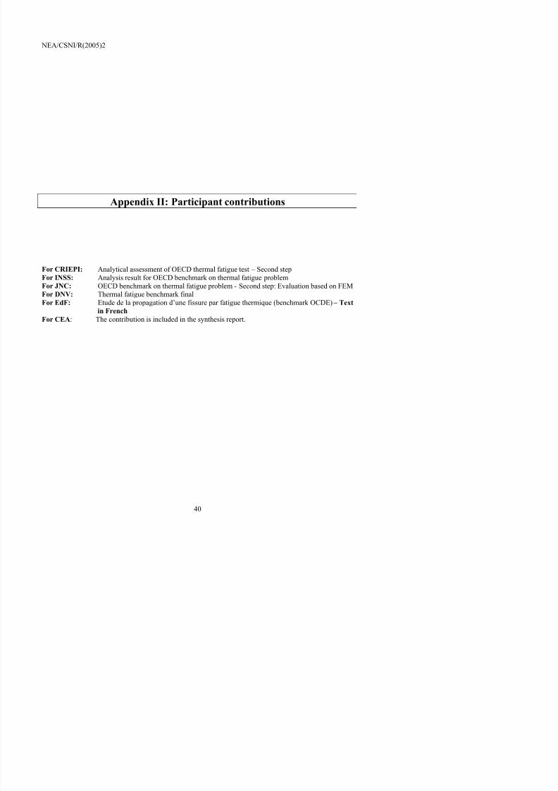
7/31/2019 Nea Study of Thermal Fatigue
http://slidepdf.com/reader/full/nea-study-of-thermal-fatigue 40/147
NEA/CSNI/R(2005)2
Appendix II: Participant contributions
For CRIEPI: Analytical assessment of OECD thermal fatigue test – Second step For INSS: Analysis result for OECD benchmark on thermal fatigue problem For JNC: OECD benchmark on thermal fatigue problem - Second step: Evaluation based on FEMFor DNV: Thermal fatigue benchmark finalFor EdF: Etude de la propagation d’une fissure par fatigue thermique (benchmark OCDE)– Text
in FrenchFor CEA : The contribution is included in the synthesis report.
7/31/2019 Nea Study of Thermal Fatigue
http://slidepdf.com/reader/full/nea-study-of-thermal-fatigue 41/147
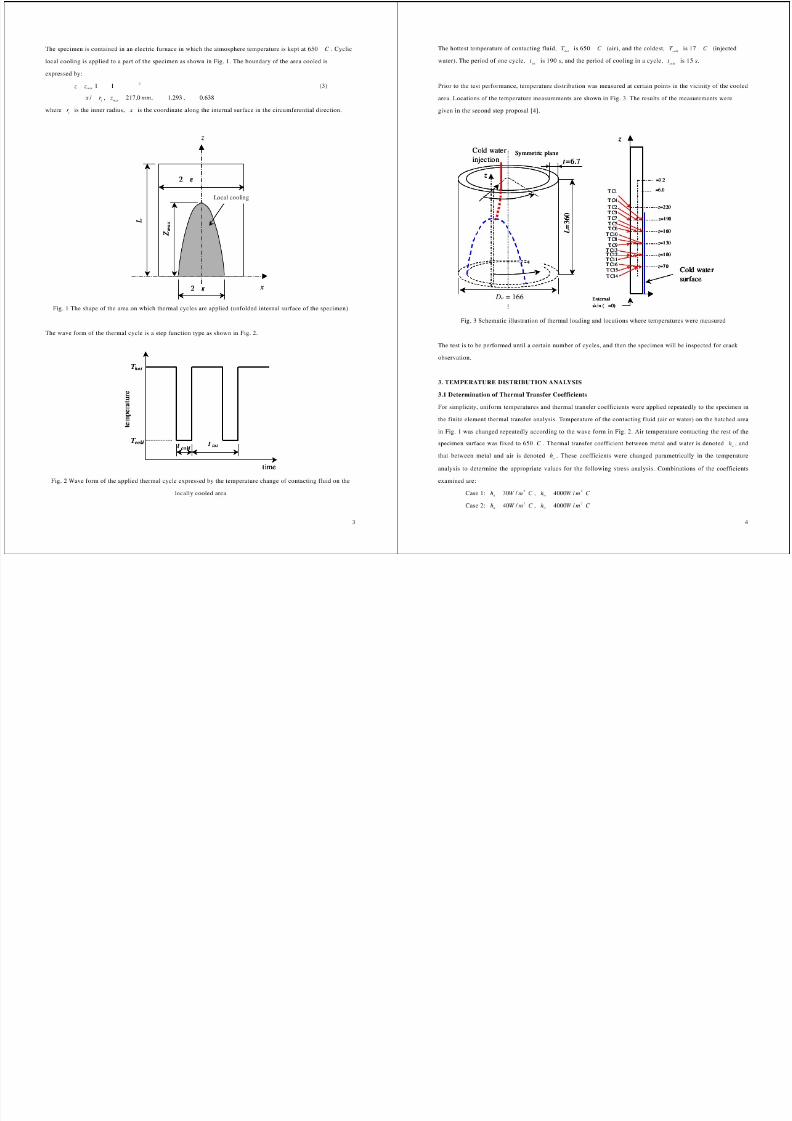
7/31/2019 Nea Study of Thermal Fatigue
http://slidepdf.com/reader/full/nea-study-of-thermal-fatigue 42/147
Case 3: C mW ha2 / 30 , C mW hw
2 / 5000600600
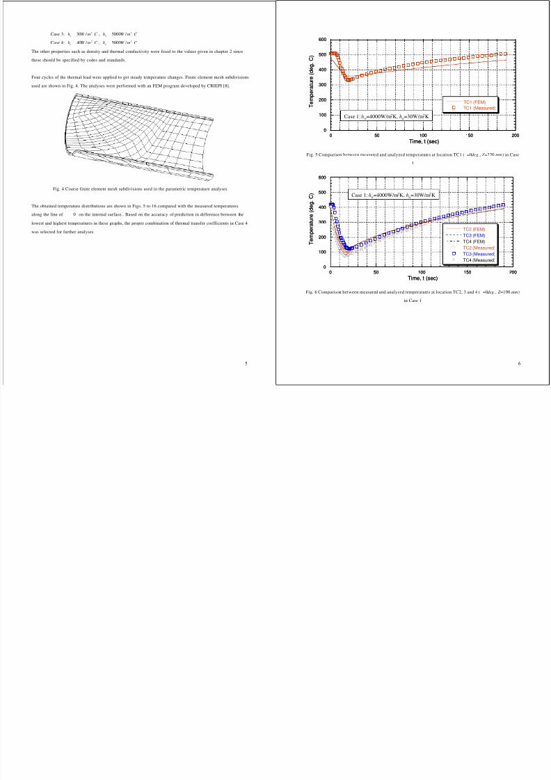
7/31/2019 Nea Study of Thermal Fatigue
http://slidepdf.com/reader/full/nea-study-of-thermal-fatigue 43/147
5
Case 4: C mW ha2 / 40 , C mW hw
2 / 5000
The other properties such as density and thermal conductivity were fixed to the values given in chapter 2 since
these should be specified by codes and standards.
Four cycles of the thermal load were applied to get steady temperature changes. Finite element mesh subdivisions
used are shown in Fig. 4. The analyses were performed with an FEM program developed by CRIEPI [8].
Fig. 4 Coarse finite element mesh subdivisions used in the parametric temperature analyses
The obtained temperature distributions are shown in Figs. 5 to 16 compared with the measured temperatures
along the line of 0 on the internal surface.. Based on the accuracy of prediction in difference between the
lowest and highest temperatures in these graphs, the proper combination of thermal transfer coefficients in Case 4
was selected for further analyses.
6
0
100
200
300
400
500
600
0 50 100 150 200
TC1 (FEM)TC1 (Measured)
T e m p e r a
t u r e (
d e g .
C )
Time, t (sec)
Case 1: hw=4000W/m 2K, ha=30W/m 2K
0
100
200
300
400
500
600
0 50 100 150 200
TC1 (FEM)TC1 (Measured)
T e m p e r a
t u r e (
d e g .
C )
Time, t (sec)
Case 1: hw=4000W/m 2K, ha=30W/m 2K
Fig. 5 Comparison between measured and analyzed temperatures at location TC1 ( =0 deg. , Z =220 mm) in Case
1
0
100
200
300
400
500
600
0 50 100 150 200
TC2 (FEM)TC3 (FEM)TC4 (FEM)TC2 (Measured)TC3 (Measured)TC4 (Measured)
T e m p e r a
t u r e ( d
e g .
C )
Time, t (sec)
Case 1: hw=4000W/m 2K, ha =30W/m 2K
0
100
200
300
400
500
600
0 50 100 150 200
TC2 (FEM)TC3 (FEM)TC4 (FEM)TC2 (Measured)TC3 (Measured)TC4 (Measured)
T e m p e r a
t u r e ( d
e g .
C )
Time, t (sec)
Case 1: hw=4000W/m 2K, ha =30W/m 2K
Fig. 6 Comparison between measured and analyzed temperatures at location TC2, 3 and 4 ( =0 deg ., Z =190 mm)
in Case 1
600600
600600
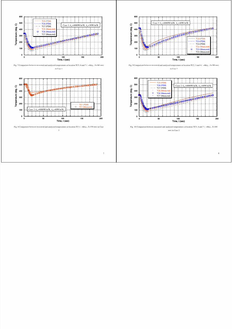
7/31/2019 Nea Study of Thermal Fatigue
http://slidepdf.com/reader/full/nea-study-of-thermal-fatigue 44/147
7
0
100
200
300
400
500
600
0 50 100 150 200
TC5 (FEM)TC6 (FEM)TC7 (FEM)TC5 (Measured)
TC6 (Measured)TC7 (Measured)
T e m p e r a
t u r e
( d e g .
C )
Time, t (sec)
Case 1: hw=4000W/m 2K, ha=30W/m 2K
0
100
200
300
400
500
600
0 50 100 150 200
TC5 (FEM)TC6 (FEM)TC7 (FEM)TC5 (Measured)
TC6 (Measured)TC7 (Measured)
T e m p e r a
t u r e
( d e g .
C )
Time, t (sec)
Case 1: hw=4000W/m 2K, ha=30W/m 2K
Fig. 7 Comparison between measured and analyzed temperatures at location TC5, 6 and 7 ( =0 deg ., Z =160 mm)
in Case 1
0
100
200
300
400
500
600
0 50 100 150 200
TC1 (FEM)TC1 (Measured)
T e m p e r a
t u r e
( d e g .
C )
Time, t (sec)
Case 2: hw=4000W/m 2K, ha =40W/m 2K
0
100
200
300
400
500
600
0 50 100 150 200
TC1 (FEM)TC1 (Measured)
T e m p e r a
t u r e
( d e g .
C )
Time, t (sec)
Case 2: hw=4000W/m 2K, ha =40W/m 2K
Fig. 8 Comparison between measured and analyzed temperatures at location TC1 ( =0 deg. , Z =220 mm) in Case
2
8
0
100
200
300
400
500
600
0 50 100 150 200
TC2 (FEM)TC3 (FEM)TC4 (FEM)TC2 (Measured)TC3 (Measured)TC4 (Measured)
T e m p e r a
t u r e
( d e g .
C )
Time, t (sec)
Case 2: hw=4000W/m 2K, ha =40W/m 2K
0
100
200
300
400
500
600
0 50 100 150 200
TC2 (FEM)TC3 (FEM)TC4 (FEM)TC2 (Measured)TC3 (Measured)TC4 (Measured)
T e m p e r a
t u r e
( d e g .
C )
Time, t (sec)
Case 2: hw=4000W/m 2K, ha =40W/m 2K
Fig. 9 Comparison between measured and analyzed temperatures at location TC2, 3 and 4 ( =0 deg ., Z =190 mm)
in Case 2
0
100
200
300
400
500
600
0 50 100 150 200
TC5 (FEM)TC6 (FEM)
TC7 (FEM)TC5 (Measured)TC6 (Measured)TC7 (Measured)
T e m p e r a
t u r e
( d e g .
C )
Time, t (sec)
Case 2: hw=4000W/m 2K, ha=40W/m 2K
0
100
200
300
400
500
600
0 50 100 150 200
TC5 (FEM)TC6 (FEM)
TC7 (FEM)TC5 (Measured)TC6 (Measured)TC7 (Measured)
T e m p e r a
t u r e
( d e g .
C )
Time, t (sec)
Case 2: hw=4000W/m 2K, ha=40W/m 2K
Fig. 10 Comparison between measured and analyzed temperatures at location TC5, 6 and 7 ( =0 deg ., Z =160
mm) in Case 2
600600
600600
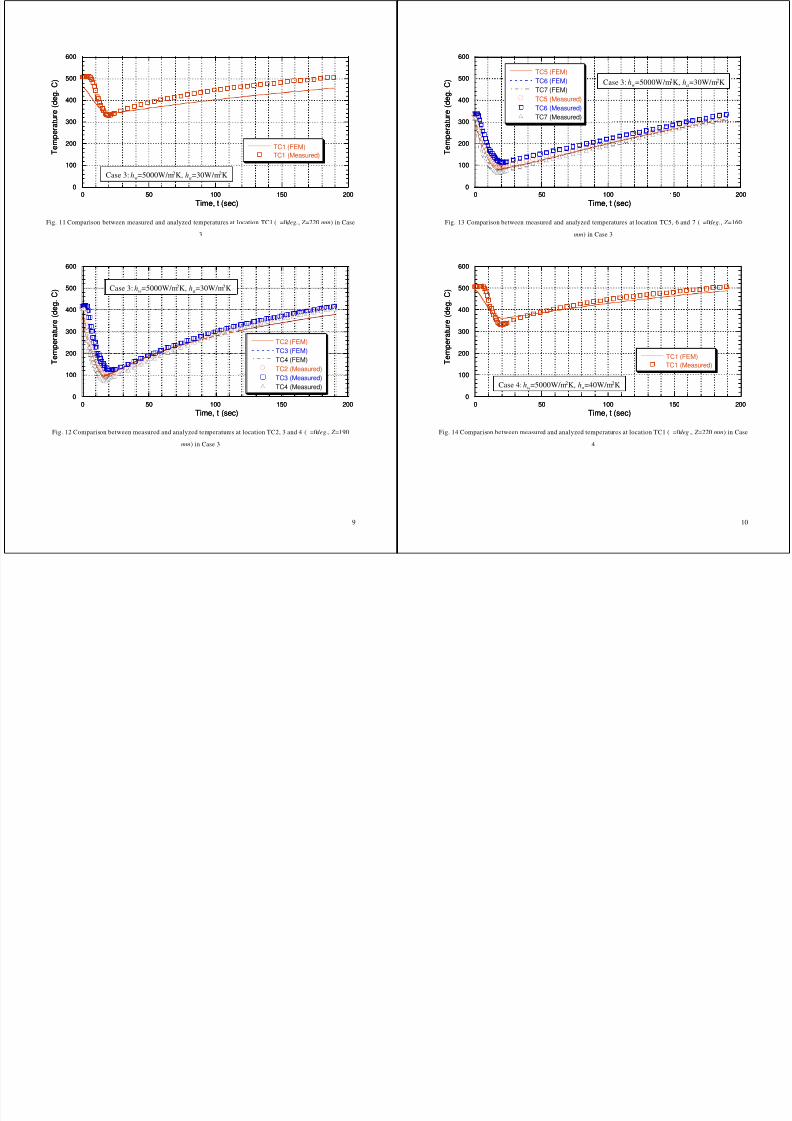
7/31/2019 Nea Study of Thermal Fatigue
http://slidepdf.com/reader/full/nea-study-of-thermal-fatigue 45/147
9
0
100
200
300
400
500
0 50 100 150 200
TC1 (FEM)TC1 (Measured)
T e m p e r a
t u r e
( d e g .
C )
Time, t (sec)
Case 3: hw=5000W/m 2K, ha =30W/m 2K
0
100
200
300
400
500
0 50 100 150 200
TC1 (FEM)TC1 (Measured)
T e m p e r a
t u r e
( d e g .
C )
Time, t (sec)
Case 3: hw=5000W/m 2K, ha =30W/m 2K
Fig. 11 Comparison between measured and analyzed temperatures at location TC1 ( =0 deg. , Z =220 mm) in Case
3
0
100
200
300
400
500
600
0 50 100 150 200
TC2 (FEM)TC3 (FEM)TC4 (FEM)TC2 (Measured)TC3 (Measured)TC4 (Measured)
T e m p e r a
t u r e
( d e g .
C )
Time, t (sec)
Case 3: hw=5000W/m 2K, ha=30W/m 2K
0
100
200
300
400
500
600
0 50 100 150 200
TC2 (FEM)TC3 (FEM)TC4 (FEM)TC2 (Measured)TC3 (Measured)TC4 (Measured)
T e m p e r a
t u r e
( d e g .
C )
Time, t (sec)
Case 3: hw=5000W/m 2K, ha=30W/m 2K
Fig. 12 Comparison between measured and analyzed temperatures at location TC2, 3 and 4 ( =0 deg., Z =190
mm) in Case 3
10
0
100
200
300
400
500
0 50 100 150 200
TC5 (FEM)TC6 (FEM)TC7 (FEM)TC5 (Measured)
TC6 (Measured)TC7 (Measured)
T e m p e r a
t u r e
( d e g .
C )
Time, t (sec)
Case 3: hw=5000W/m 2K, ha =30W/m 2K
0
100
200
300
400
500
0 50 100 150 200
TC5 (FEM)TC6 (FEM)TC7 (FEM)TC5 (Measured)
TC6 (Measured)TC7 (Measured)
T e m p e r a
t u r e
( d e g .
C )
Time, t (sec)
Case 3: hw=5000W/m 2K, ha =30W/m 2K
Fig. 13 Comparison between measured and analyzed temperatures at location TC5, 6 and 7 ( =0 deg. , Z =160
mm) in Case 3
0
100
200
300
400
500
600
0 50 100 150 200
TC1 (FEM)TC1 (Measured)
T e m p e r a
t u r e
( d e g .
C )
Time, t (sec)
Case 4: hw=5000W/m 2K, ha=40W/m 2K
0
100
200
300
400
500
600
0 50 100 150 200
TC1 (FEM)TC1 (Measured)
T e m p e r a
t u r e
( d e g .
C )
Time, t (sec)
Case 4: hw=5000W/m 2K, ha=40W/m 2K
Fig. 14 Comparison between measured and analyzed temperatures at location TC1 ( =0 deg ., Z =220 mm) in Case
4
600600
temperature changes at location TC1 in Fig. 18 was slightly improved from Fig. 14. Then the results from this
analysis were used for stress analysis in the following chapter
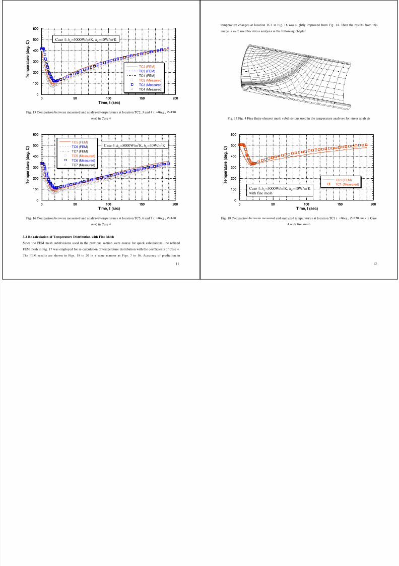
7/31/2019 Nea Study of Thermal Fatigue
http://slidepdf.com/reader/full/nea-study-of-thermal-fatigue 46/147
11
0
100
200
300
400
500
0 50 100 150 200
TC2 (FEM)TC3 (FEM)TC4 (FEM)TC2 (Measured)TC3 (Measured)TC4 (Measured)
T e m p e r a
t u r e
( d e g .
C )
Time, t (sec)
Case 4: hw=5000W/m 2K, ha=40W/m 2K
0
100
200
300
400
500
0 50 100 150 200
TC2 (FEM)TC3 (FEM)TC4 (FEM)TC2 (Measured)TC3 (Measured)TC4 (Measured)
T e m p e r a
t u r e
( d e g .
C )
Time, t (sec)
Case 4: hw=5000W/m 2K, ha=40W/m 2K
Fig. 15 Comparison between measured and analyzed temperatures at location TC2, 3 and 4 ( =0 deg ., Z =190
mm) in Case 4
0
100
200
300
400
500
600
0 50 100 150 200
TC5 (FEM)TC6 (FEM)TC7 (FEM)TC5 (Measured)TC6 (Measured)TC7 (Measured)
T e m p e r a
t u r e
( d e g .
C )
Time, t (sec)
Case 4: hw=5000W/m 2K, ha =40W/m 2K
0
100
200
300
400
500
600
0 50 100 150 200
TC5 (FEM)TC6 (FEM)TC7 (FEM)TC5 (Measured)TC6 (Measured)TC7 (Measured)
T e m p e r a
t u r e
( d e g .
C )
Time, t (sec)
Case 4: hw=5000W/m 2K, ha =40W/m 2K
Fig. 16 Comparison between measured and analyzed temperatures at location TC5, 6 and 7 ( =0 deg ., Z =160
mm) in Case 4
3.2 Re-calculation of Temperature Distribution with Fine Mesh
Since the FEM mesh subdivisions used in the previous section were coarse for quick calculations, the refined
FEM mesh in Fig. 17 was employed for re-calculation of temperature distribution with the coefficients of Case 4.
The FEM results are shown in Figs. 18 to 20 in a same manner as Figs. 7 to 16. Accuracy of prediction in
12
analysis were used for stress analysis in the following chapter.
Fig. 17 Fig. 4 Fine finite element mesh subdivisions used in the temperature analyses for stress analysis
0
100
200
300
400
500
600
0 50 100 150 200
TC1 (FEM)TC1 (Measured)
T e m p e r a
t u r e
( d e g .
C )
Time, t (sec)
Case 4: hw=5000W/m 2K, ha=40W/m 2Kwith fine mesh
0
100
200
300
400
500
600
0 50 100 150 200
TC1 (FEM)TC1 (Measured)
T e m p e r a
t u r e
( d e g .
C )
Time, t (sec)
Case 4: hw=5000W/m 2K, ha=40W/m 2Kwith fine mesh
Fig. 18 Comparison between measured and analyzed temperatures at location TC1 ( =0 deg. , Z =220 mm) in Case
4 with fine mesh
600600
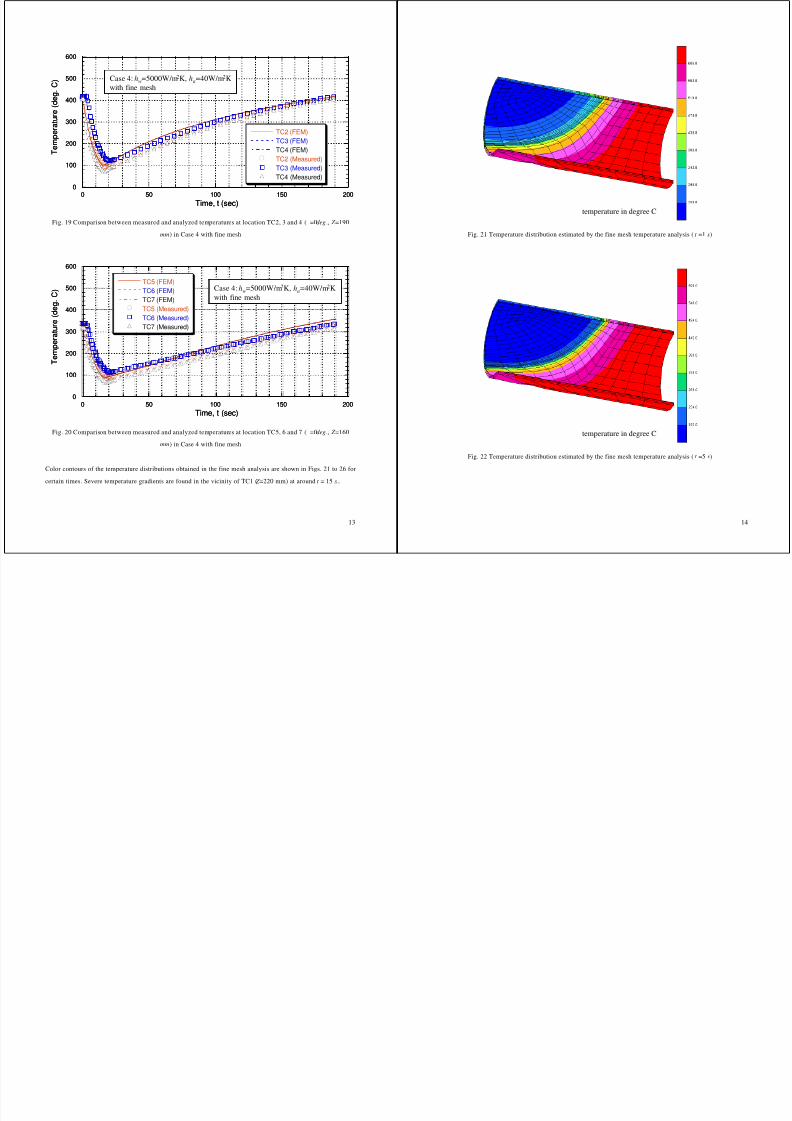
7/31/2019 Nea Study of Thermal Fatigue
http://slidepdf.com/reader/full/nea-study-of-thermal-fatigue 47/147
13
0
100
200
300
400
500
0 50 100 150 200
TC2 (FEM)TC3 (FEM)TC4 (FEM)TC2 (Measured)TC3 (Measured)TC4 (Measured)
T e m p e r a
t u r e
( d e g .
C )
Time, t (sec)
Case 4: hw=5000W/m 2K, ha=40W/m 2Kwith fine mesh
0
100
200
300
400
500
0 50 100 150 200
TC2 (FEM)TC3 (FEM)TC4 (FEM)TC2 (Measured)TC3 (Measured)TC4 (Measured)
T e m p e r a
t u r e
( d e g .
C )
Time, t (sec)
Case 4: hw=5000W/m 2K, ha=40W/m 2Kwith fine mesh
Fig. 19 Comparison between measured and analyzed temperatures at location TC2, 3 and 4 ( =0 deg ., Z =190
mm) in Case 4 with fine mesh
0
100
200
300
400
500
600
0 50 100 150 200
TC5 (FEM)TC6 (FEM)TC7 (FEM)TC5 (Measured)TC6 (Measured)TC7 (Measured)
T e m p e r a
t u r e
( d e g .
C )
Time, t (sec)
Case 4: hw=5000W/m 2K, ha =40W/m 2Kwith fine mesh
0
100
200
300
400
500
600
0 50 100 150 200
TC5 (FEM)TC6 (FEM)TC7 (FEM)TC5 (Measured)TC6 (Measured)TC7 (Measured)
T e m p e r a
t u r e
( d e g .
C )
Time, t (sec)
Case 4: hw=5000W/m 2K, ha =40W/m 2Kwith fine mesh
Fig. 20 Comparison between measured and analyzed temperatures at location TC5, 6 and 7 ( =0 deg ., Z =160
mm) in Case 4 with fine mesh
Color contours of the temperature distributions obtained in the fine mesh analysis are shown in Figs. 21 to 26 for
certain times. Severe temperature gradients are found in the vicinity of TC1 ( Z =220 mm) at around t = 15 s ..
14
temperature in degree Ctemperature in degree C
Fig. 21 Temperature distribution estimated by the fine mesh temperature analysis ( t =1 s)
temperature in degree Ctemperature in degree C
Fig. 22 Temperature distribution estimated by the fine mesh temperature analysis ( t =5 s)
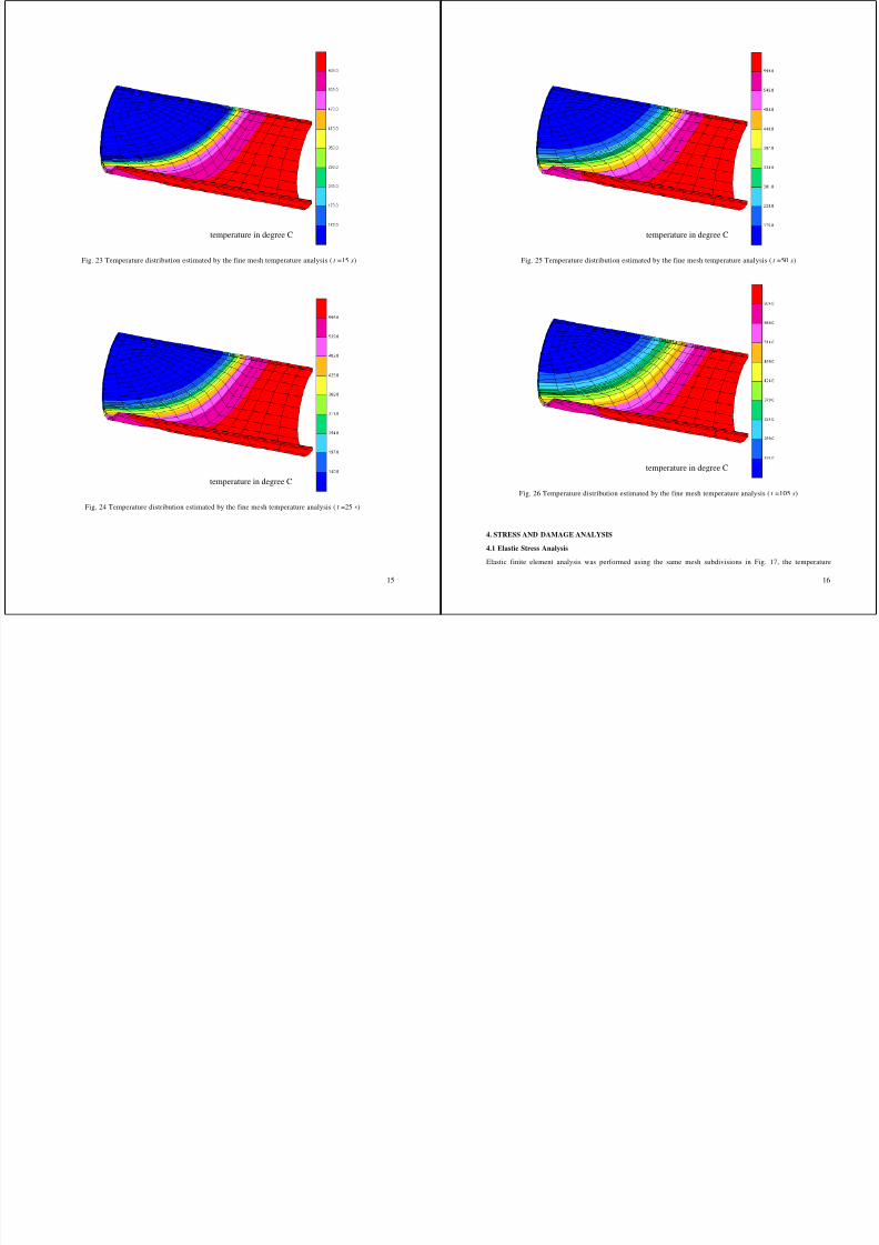
7/31/2019 Nea Study of Thermal Fatigue
http://slidepdf.com/reader/full/nea-study-of-thermal-fatigue 48/147
15
temperature in degree Ctemperature in degree C
Fig. 23 Temperature distribution estimated by the fine mesh temperature analysis ( t =15 s)
temperature in degree Ctemperature in degree C
Fig. 24 Temperature distribution estimated by the fine mesh temperature analysis ( t =25 s)
16
temperature in degree Ctemperature in degree C
Fig. 25 Temperature distribution estimated by the fine mesh temperature analysis ( t =50 s)
temperature in degree Ctemperature in degree C
Fig. 26 Temperature distribution estimated by the fine mesh temperature analysis ( t =105 s)
4. STRESS AND DAMAGE ANALYSIS
4.1 Elastic Stress Analysis
Elastic finite element analysis was performed using the same mesh subdivisions in Fig. 17, the temperature
distributions obtained in section 3.2 and the material properties in chapter 2. The analysis was performed with
also the CRIEPI's FEM code [8].
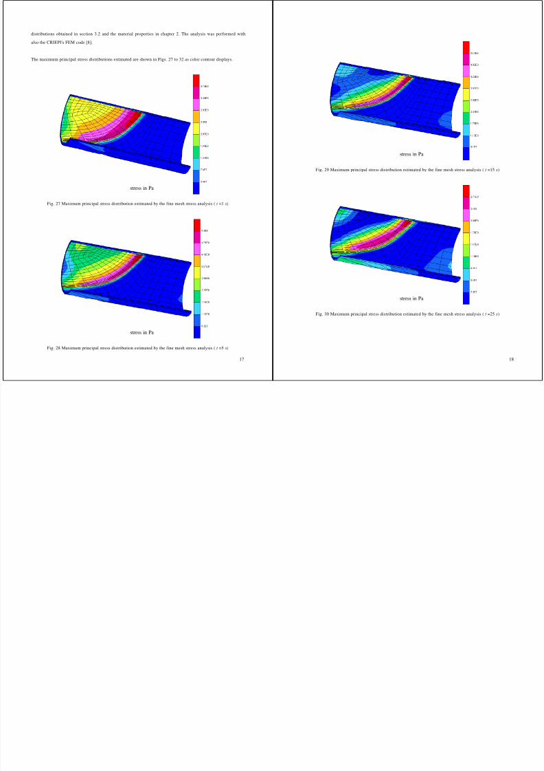
7/31/2019 Nea Study of Thermal Fatigue
http://slidepdf.com/reader/full/nea-study-of-thermal-fatigue 49/147
17
The maximum principal stress distributions estimated are shown in Figs. 27 to 32 as color contour displays.
stress in Pastress in Pa
Fig. 27 Maximum principal stress distribution estimated by the fine mesh stress analysis ( t =1 s)
stress in Pastress in Pa
Fig. 28 Maximum principal stress distribution estimated by the fine mesh stress analysis ( t =5 s)
18
stress in Pastress in Pa
Fig. 29 Maximum principal stress distribution estimated by the fine mesh stress analysis ( t =15 s)
stress in Pastress in Pa
Fig. 30 Maximum principal stress distribution estimated by the fine mesh stress analysis ( t =25 s)
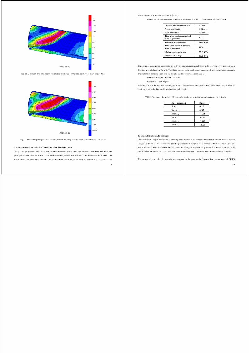
7/31/2019 Nea Study of Thermal Fatigue
http://slidepdf.com/reader/full/nea-study-of-thermal-fatigue 50/147
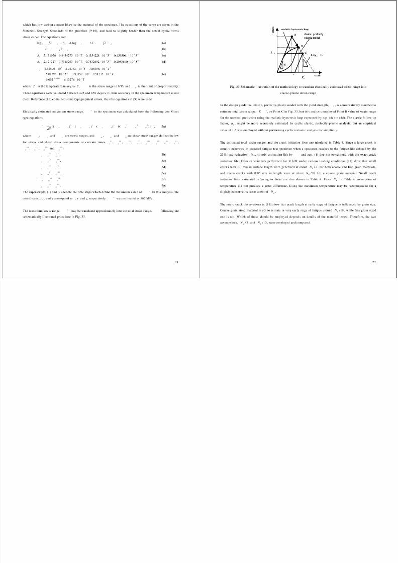
7/31/2019 Nea Study of Thermal Fatigue
http://slidepdf.com/reader/full/nea-study-of-thermal-fatigue 51/147
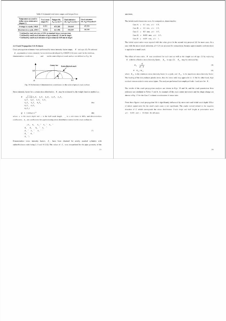
7/31/2019 Nea Study of Thermal Fatigue
http://slidepdf.com/reader/full/nea-study-of-thermal-fatigue 52/147
1
/ w
10
at penetration initial depth=0.5 mm (R=0)
10
at penetration initial depth=0.5 mm (R=0)
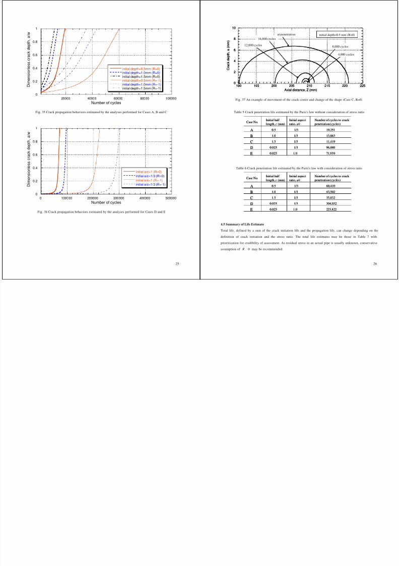
7/31/2019 Nea Study of Thermal Fatigue
http://slidepdf.com/reader/full/nea-study-of-thermal-fatigue 53/147
25
0
0.2
0.4
0.6
0.8
20000 40000 60000 80000 100000
initial depth=0.5mm (R=0)initial depth=1.0mm (R=0)initial depth=1.5mm (R=0)initial depth=0.5mm (R=-1)initial depth=1.0mm (R=-1)initial depth=1.5mm (R=-1)
D i m e n s
i o n
l e s s c r a c
k d e p
t h ,
a
Number of cycles
Fig. 35 Crack propagation behaviors estimated by the analyses performed for Cases A, B and C
0
0.2
0.4
0.6
0.8
1
0 100000 200000 300000 400000 500000
initial a/c=1 (R=0)initial a/c=1/3 (R=0)initial a/c=1 (R=-1)initial a/c=1/3 (R=-1) D
i m e n s i o n
l e s s c r a c
k d e p
t h ,
a / w
Number of cycles
Fig. 36 Crack propagation behaviors estimated by the analyses performed for Cases D and E
26
0
2
4
6
8
190 195 200 205 210 215 220 225
C r a c
k d e p
t h ,
a ( m m
)
Axial distance, Z (mm)
4,000 cycles
8,000 cycles12,000 cycles
16,000 cyclesp t a dept 0.5 ( 0)
0
2
4
6
8
190 195 200 205 210 215 220 225
C r a c
k d e p
t h ,
a ( m m
)
Axial distance, Z (mm)
4,000 cycles
8,000 cycles12,000 cycles
16,000 cyclesp t a dept 0.5 ( 0)
Fig. 37 An example of movement of the crack center and change of the shape (Case C, R=0)
Table 5 Crack penetration life estimated by the Paris's law without consideration of stress ratio
Number of cycles to crack penetration (cycles)
Case No.Initial half length, c (mm)
A
B
C
D
E
Initial aspectratio, a/c
0.5
1.0
1.5
0.025
0.025
1/3
1/3
1/3
1/3
1.0 71,959
96,880
19,251
13,863
11,419
Number of cycles to crack penetration (cycles)
Case No.Initial half length, c (mm)
A
B
C
D
E
Initial aspectratio, a/c
0.5
1.0
1.5
0.025
0.025
1/3
1/3
1/3
1/3
1.0 71,959
96,880
19,251
13,863
11,419
Table 6 Crack penetration life estimated by the Paris's law with consideration of stress ratio
Number of cycles to crack penetration (cycles)
Case No.Initial half length, c (mm)
A
B
C
DE
Initial aspectratio, a/c
0.5
1.0
1.5
0.025
0.025
1/3
1/3
1/3
1/3
1.0 225,822
304,032
60,410
43,502
35,832
Number of cycles to crack penetration (cycles)
Case No.Initial half length, c (mm)
A
B
C
DE
Initial aspectratio, a/c
0.5
1.0
1.5
0.025
0.025
1/3
1/3
1/3
1/3
1.0 225,822
304,032
60,410
43,502
35,832
4.5 Summary of Life Estimate
Total life, defined by a sum of the crack initiation life and the propagation life, can change depending on the
definition of crack initiation and the stress ratio. The total life estimates may be those in Table 7 with
prioritization for credibility of assessment. As residual stress in an actual pipe is usually unknown, conservative
assumption of 0 R may be recommended.
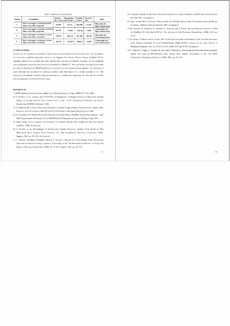
7/31/2019 Nea Study of Thermal Fatigue
http://slidepdf.com/reader/full/nea-study-of-thermal-fatigue 54/147
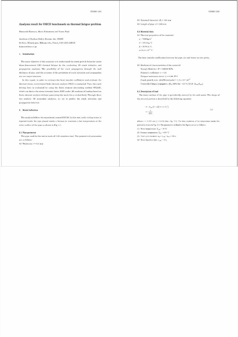
7/31/2019 Nea Study of Thermal Fatigue
http://slidepdf.com/reader/full/nea-study-of-thermal-fatigue 55/147
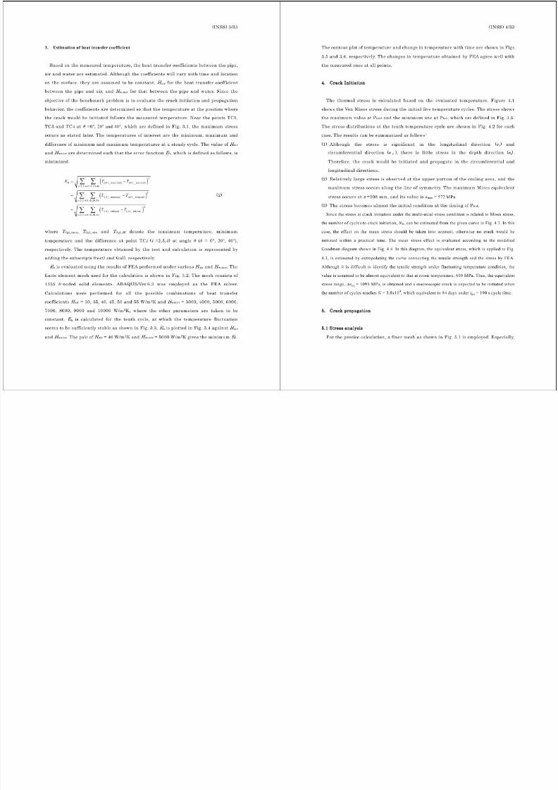
7/31/2019 Nea Study of Thermal Fatigue
http://slidepdf.com/reader/full/nea-study-of-thermal-fatigue 56/147
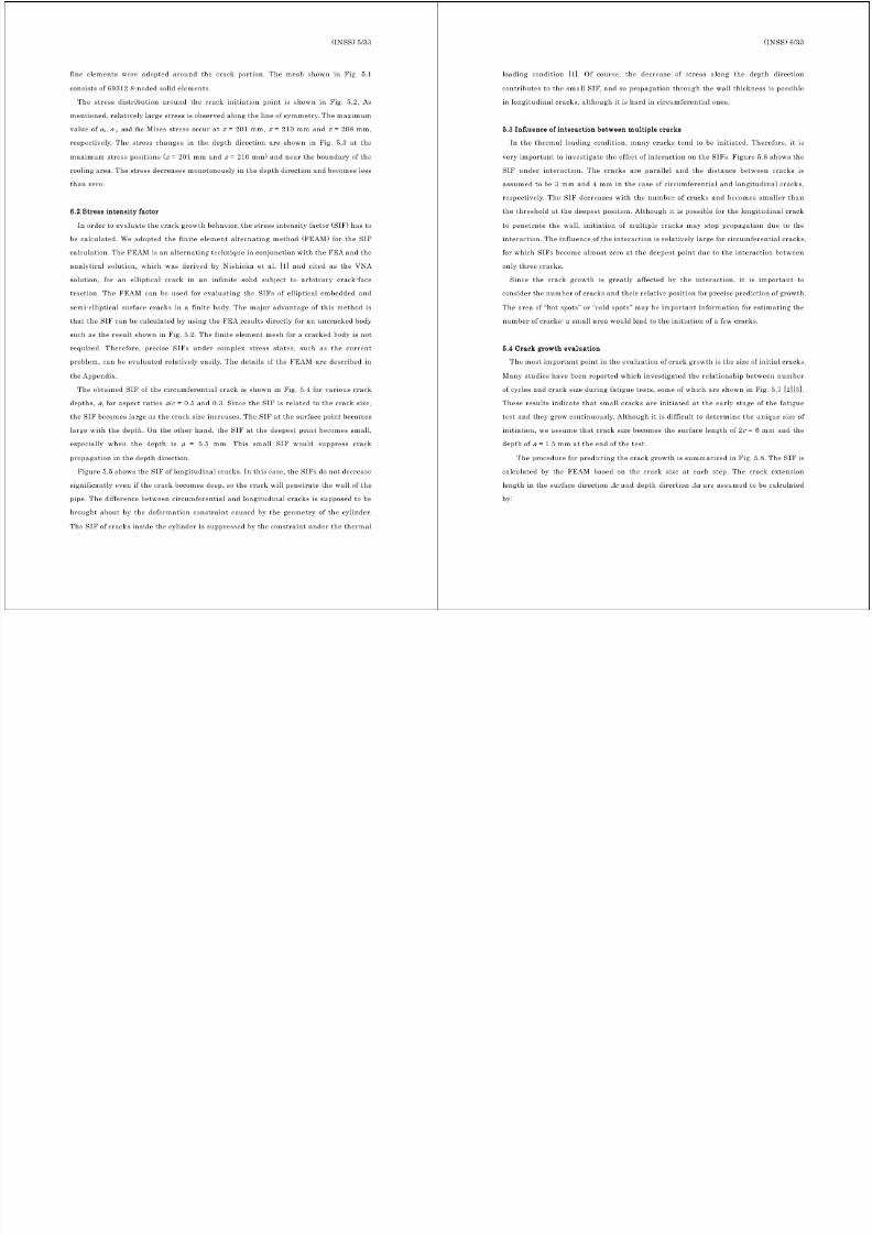
7/31/2019 Nea Study of Thermal Fatigue
http://slidepdf.com/reader/full/nea-study-of-thermal-fatigue 57/147
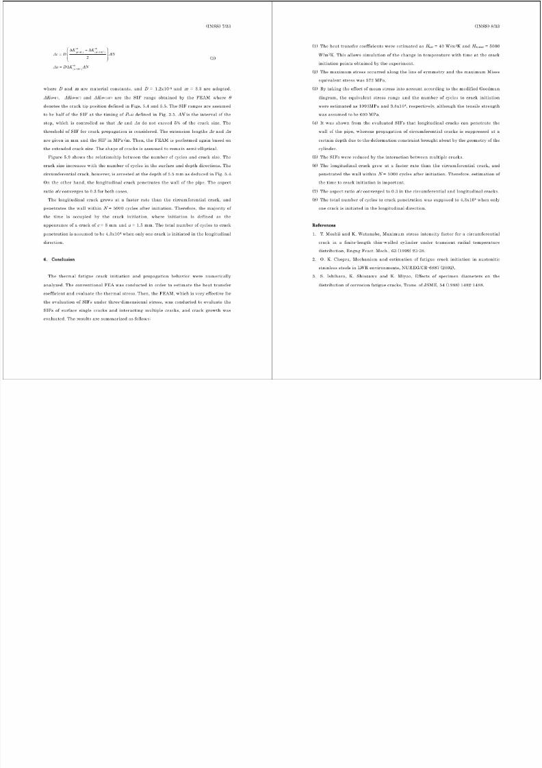
7/31/2019 Nea Study of Thermal Fatigue
http://slidepdf.com/reader/full/nea-study-of-thermal-fatigue 58/147
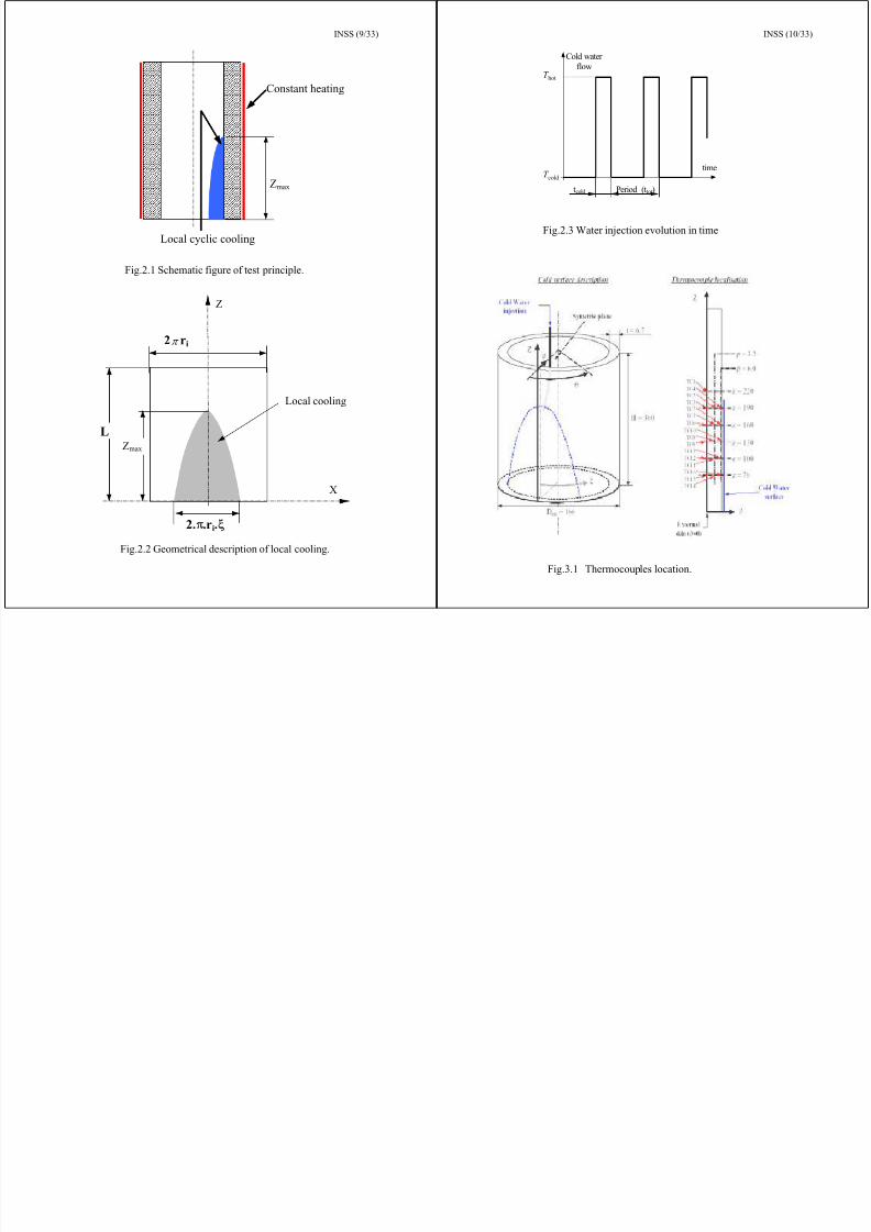
7/31/2019 Nea Study of Thermal Fatigue
http://slidepdf.com/reader/full/nea-study-of-thermal-fatigue 59/147
(INSS) 3/33
INSS (11/33)(INSS) 4/33
INSS (12/33)
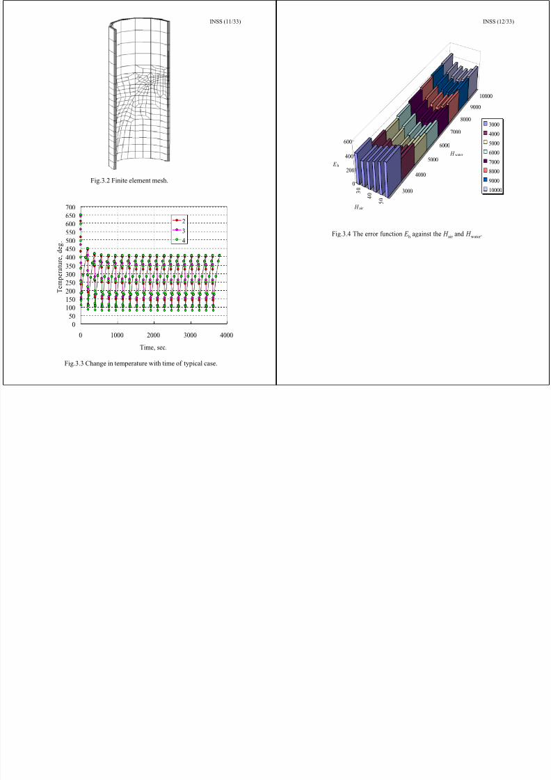
7/31/2019 Nea Study of Thermal Fatigue
http://slidepdf.com/reader/full/nea-study-of-thermal-fatigue 60/147
Fig.3.2 Finite element mesh.
050
100150200250300350400450500550600650700
0 1000 2000 3000 4000
Time, sec.
T e m p e r a t u r e ,
d e g .
234
Fig.3.3 Change in temperature with time of typical case.
3 0
4 0
5 0
3000
4000
5000
6000
7000
8000
9000
10000
0
200
400
600
4 h
; air
; water
3000
4000
50006000
7000
8000
9000
10000
Fig.3.4 The error function 4 h against the ;
air and ; water .
(INSS) 5/33
550
650
#C
INSS (13/33)(INSS) 6/33
550
650
#C
INSS (14/33)
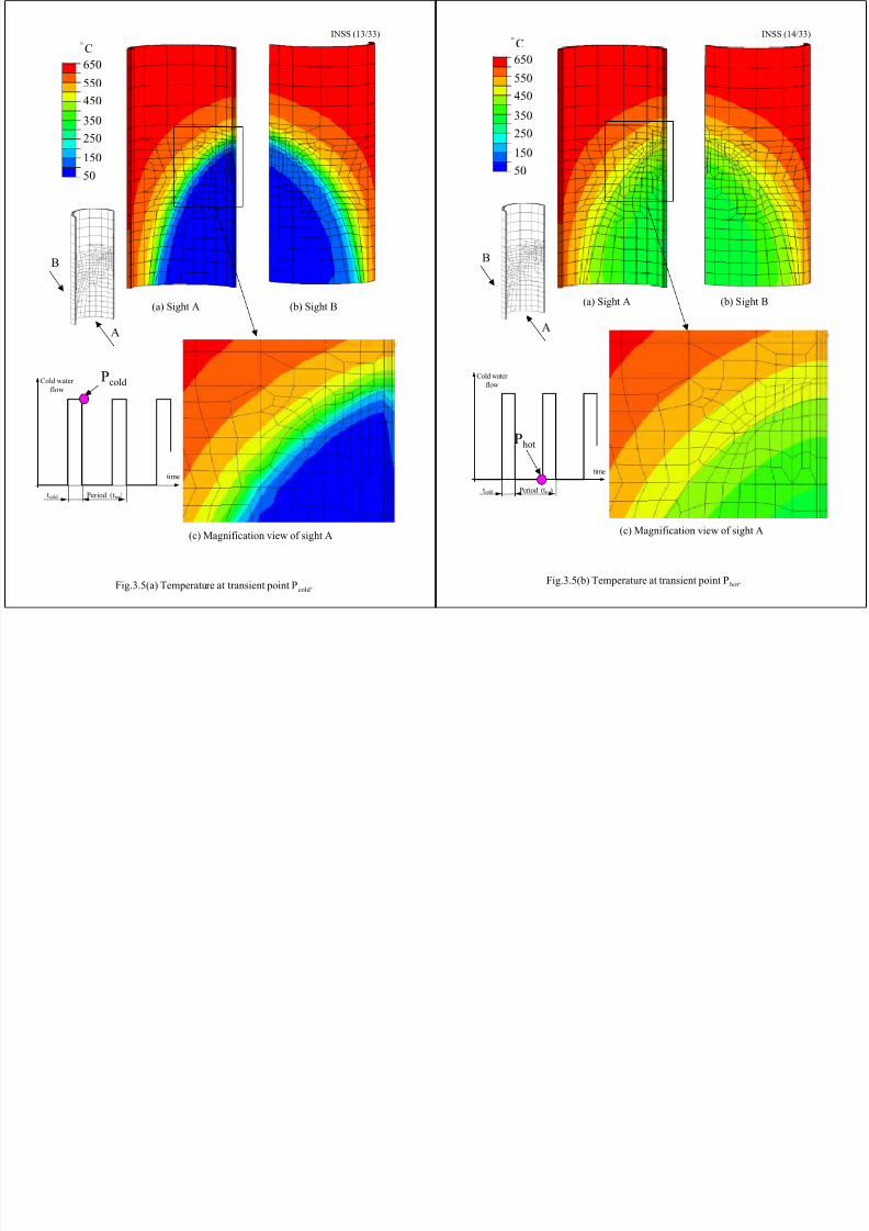
7/31/2019 Nea Study of Thermal Fatigue
http://slidepdf.com/reader/full/nea-study-of-thermal-fatigue 61/147
A
B
50150
250350
450
time
Cold water flow
tcold Period (t tot)
Pcold
(a) Sight A (b) Sight B
(c) Magnification view of sight A
Fig.3.5(a) Temperature at transient point P cold .
A
B
50150
250350
450
time
Cold water flow
tcold Period (t tot)
Phot
(a) Sight A (b) Sight B
(c) Magnification view of sight A
Fig.3.5(b) Temperature at transient point P hot.
(INSS) 7/33
INSS (15/33)
400
450
(INSS) 8/33
400
450
500
INSS (16/33)
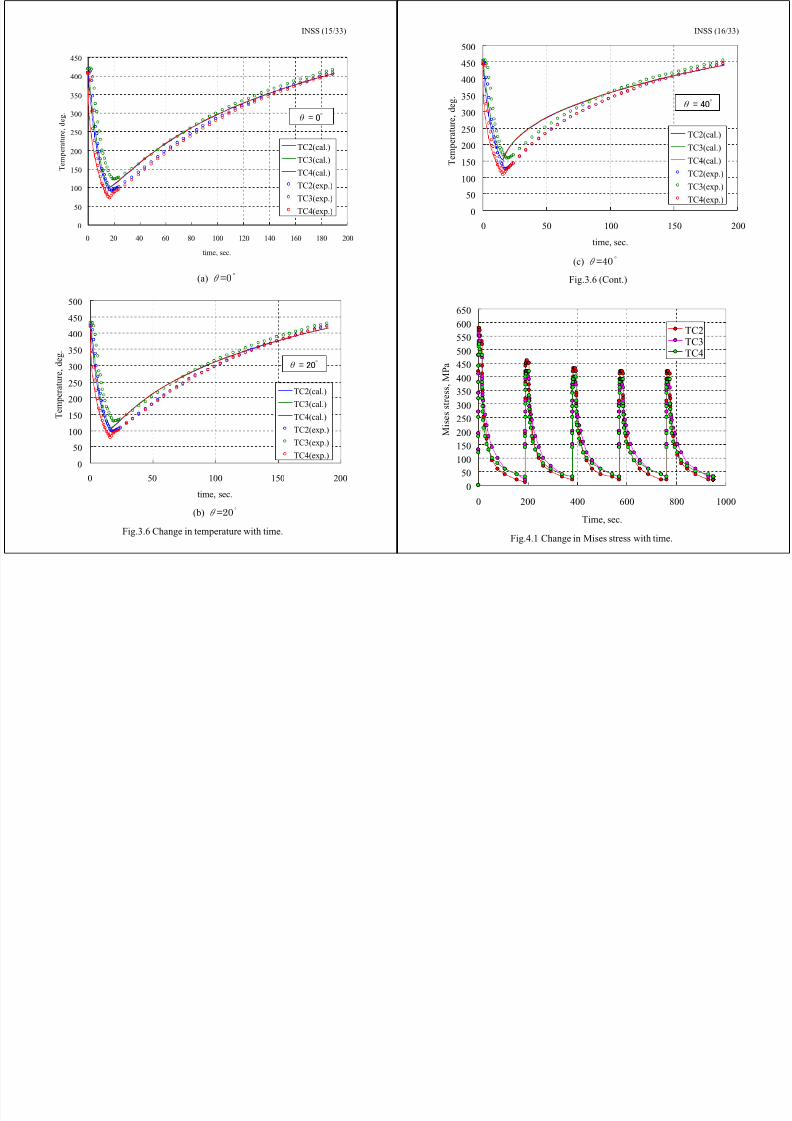
7/31/2019 Nea Study of Thermal Fatigue
http://slidepdf.com/reader/full/nea-study-of-thermal-fatigue 62/147
0
50
100
150
200
250
300
350
0 20 40 60 80 100 120 140 160 180 200
time, sec.
T e m p e r a t u r e ,
d e g .
TC2(cal.)TC3(cal.)TC4(cal.)TC2(exp.)TC3(exp.)
TC4(exp.)
2 "#"$%
(a) " =0#
0
50
100
150
200
250
300
350
400
450
500
0 50 100 150 200
time, sec.
T e m p e r a t u r e ,
d e g .
TC2(cal.)
TC3(cal.)TC4(cal.)TC2(exp.)TC3(exp.)TC4(exp.)
2 "#"&$%
(b) " =20#
Fig.3.6 Change in temperature with time.
0
50
100
150
200
250
300
350
0 50 100 150 200
time, sec.
T e m p e r a t u r e , d e g .
TC2(cal.)
TC3(cal.)
TC4(cal.)TC2(exp.)TC3(exp.)
TC4(exp.)
2 "#"'$%
(c) " =40#
Fig.3.6 (Cont.)
050
100150200250300
350400450500550600650
0 200 400 600 800 1000Time, sec.
M i s e s s t r e s s ,
M P a
TC2TC3TC4
Fig.4.1 Change in Mises stress with time.
(INSS) 9/33
500
600MPa
INSS (17/33)(INSS) 10/33
400
600MPa
INSS (18/33)
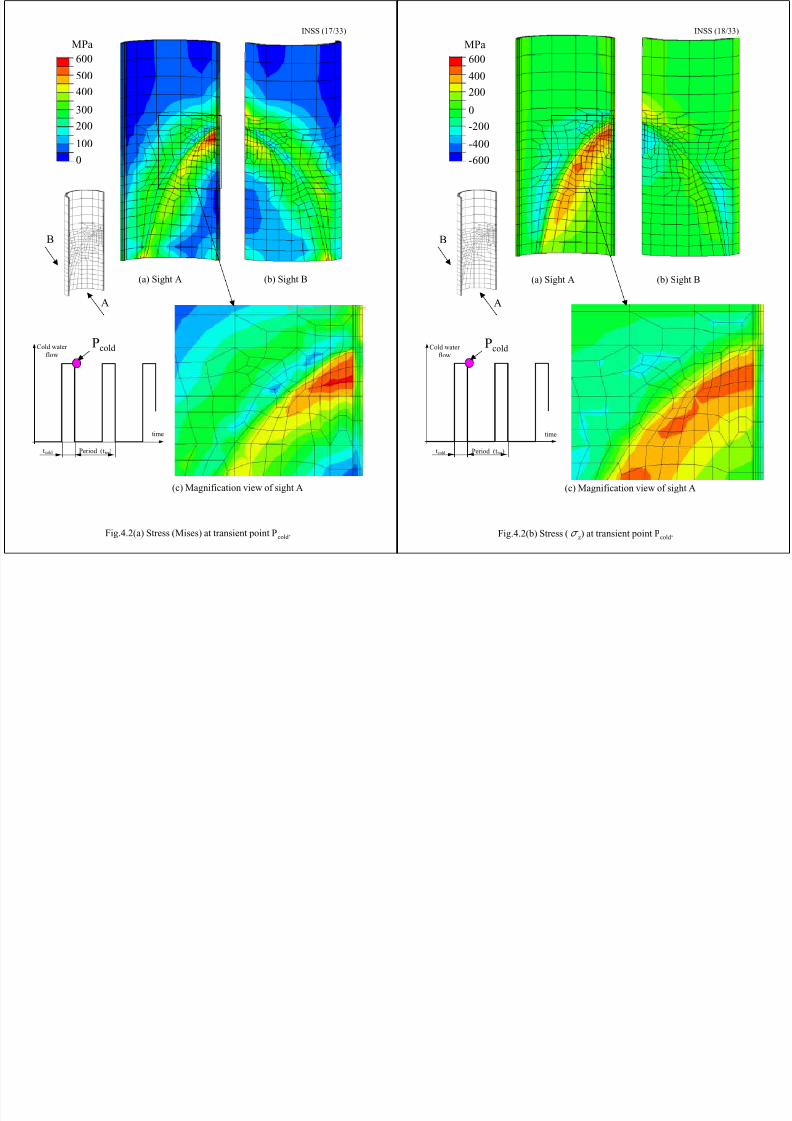
7/31/2019 Nea Study of Thermal Fatigue
http://slidepdf.com/reader/full/nea-study-of-thermal-fatigue 63/147
A
B
0100
200300
400
time
Cold water flow
tcold Period (t tot)
Pcold
(a) Sight A (b) Sight B
(c) Magnification view of sight A
Fig.4.2(a) Stress (Mises) at transient point P cold .
A
B
-600-400
-2000
200
time
Cold water flow
tcold Period (t tot)
Pcold
(a) Sight A (b) Sight B
(c) Magnification view of sight A
Fig.4.2(b) Stress ( ( z) at transient point P cold .
(INSS) 11/33
200400
600MPa
INSS (19/33)(INSS) 12/33
200400
600MPa
INSS (20/33)
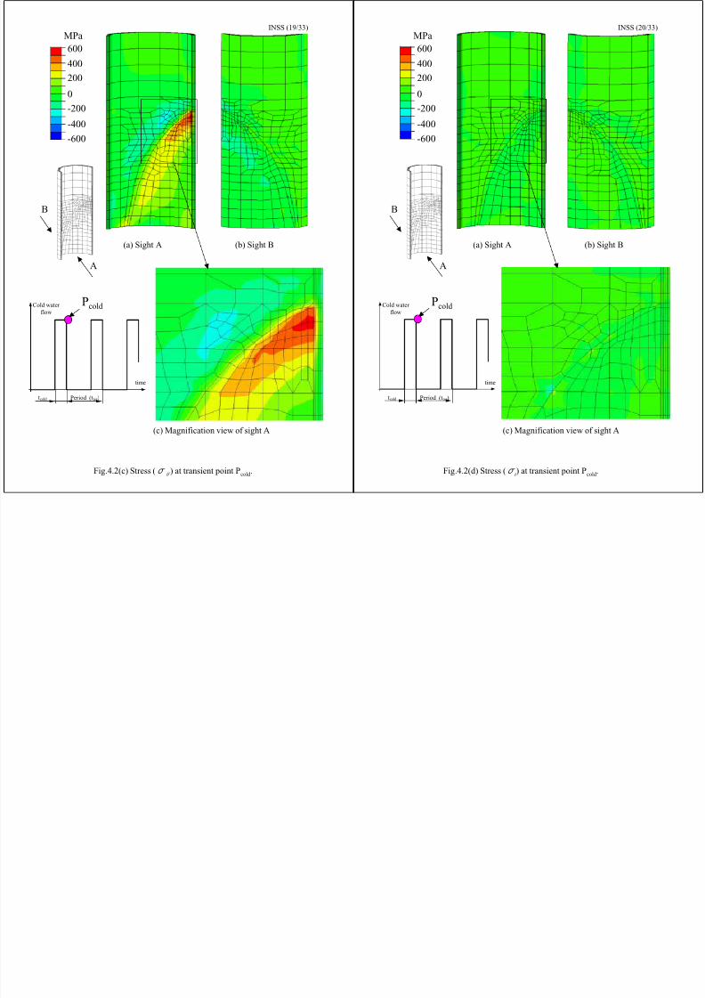
7/31/2019 Nea Study of Thermal Fatigue
http://slidepdf.com/reader/full/nea-study-of-thermal-fatigue 64/147
A
B
-600-400
-2000
200
time
Cold water flow
tcold Period (t tot)
Pcold
(a) Sight A (b) Sight B
(c) Magnification view of sight A
Fig.4.2(c) Stress ( ( " ) at transient point P cold .
A
B
-600-400
-2000
200
time
Cold water flow
tcold Period (t tot)
Pcold
(a) Sight A (b) Sight B
(c) Magnification view of sight A
Fig.4.2(d) Stress ( ( ( ) at transient point P cold .
(INSS) 13/33
400500
600MPa
INSS (21/33)(INSS) 14/33
400
600MPa
INSS (22/33)
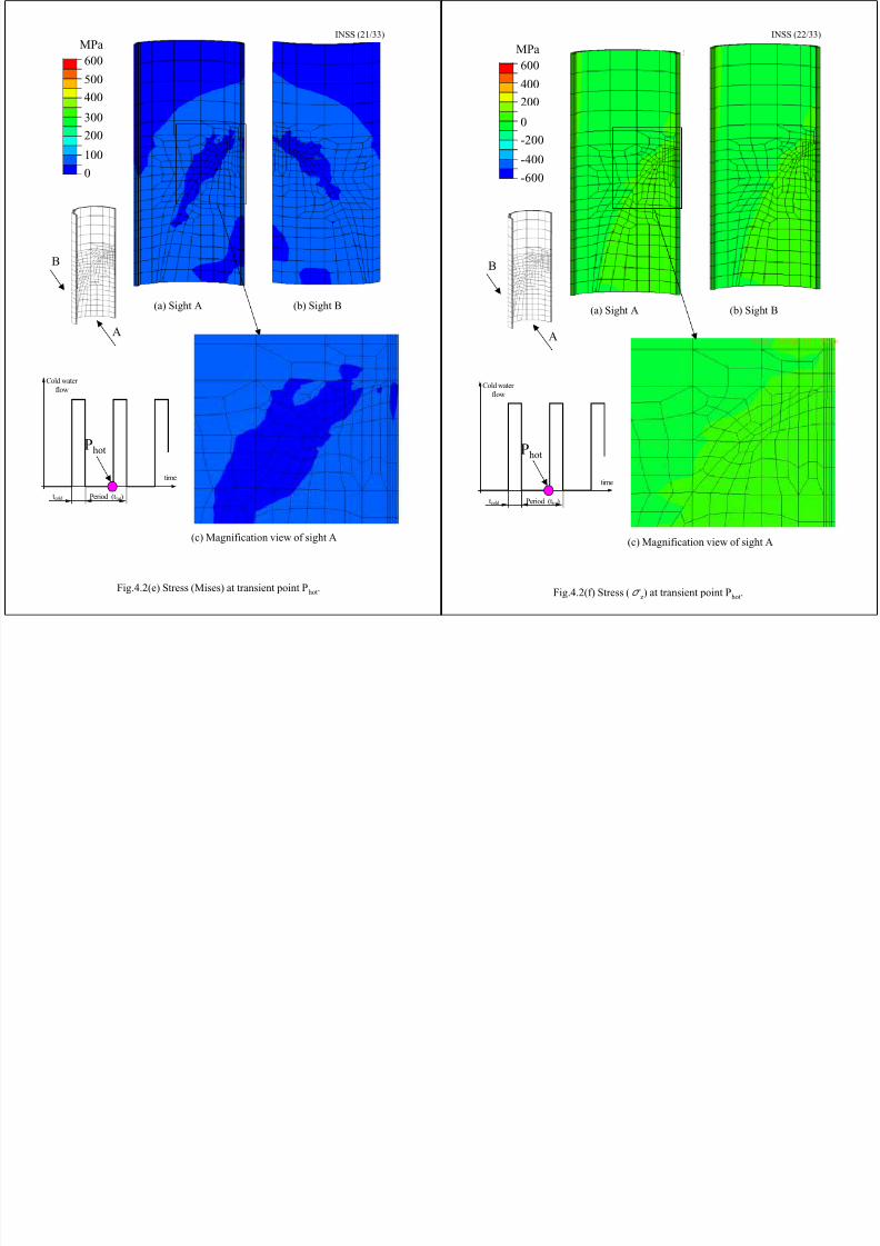
7/31/2019 Nea Study of Thermal Fatigue
http://slidepdf.com/reader/full/nea-study-of-thermal-fatigue 65/147
A
B
0100
200300
400
time
Cold water flow
tcold Period (t tot)
Phot
(a) Sight A (b) Sight B
(c) Magnification view of sight A
Fig.4.2(e) Stress (Mises) at transient point P hot.
A
B
-600-400
-2000
200
time
Cold water flow
tcold Period (t tot)
Phot
(a) Sight A (b) Sight B
(c) Magnification view of sight A
Fig.4.2(f) Stress ( ( z) at transient point P hot.
(INSS) 15/33
3000
3500
4000
P a
INSS (23/33)(INSS) 16/33
INSS (24/33)
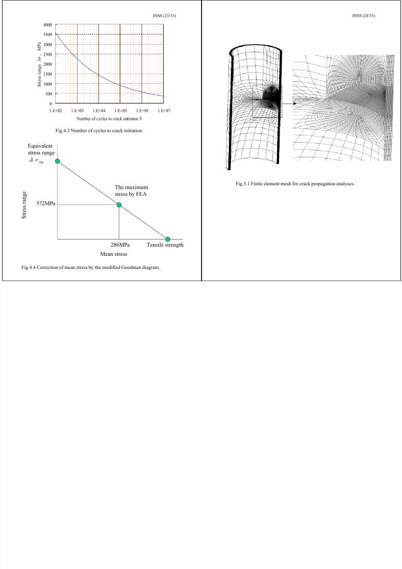
7/31/2019 Nea Study of Thermal Fatigue
http://slidepdf.com/reader/full/nea-study-of-thermal-fatigue 66/147
0
500
1000
1500
2000
2500
3000
1.E+02 1.E+03 1.E+04 1.E+05 1.E+06 1.E+07
Number of cycles to crack initiation 6
S t r e s s r a n g e
& 5
,! M P
Fig.4.3 Number of cycles to crack initiation.
Mean stress
Tensile strength
The maximumstress by FEA
572MPa
286MPa
S t r e s s r a n g e
Equivalentstress range$%
eq
Fig.4.4 Correction of mean stress by the modified Goodman diagram.
Fig.5.1 Finite element mesh for crack propagation analyses.
(INSS) 17/33
INSS (25/33)(INSS) 18/33
INSS (26/33)
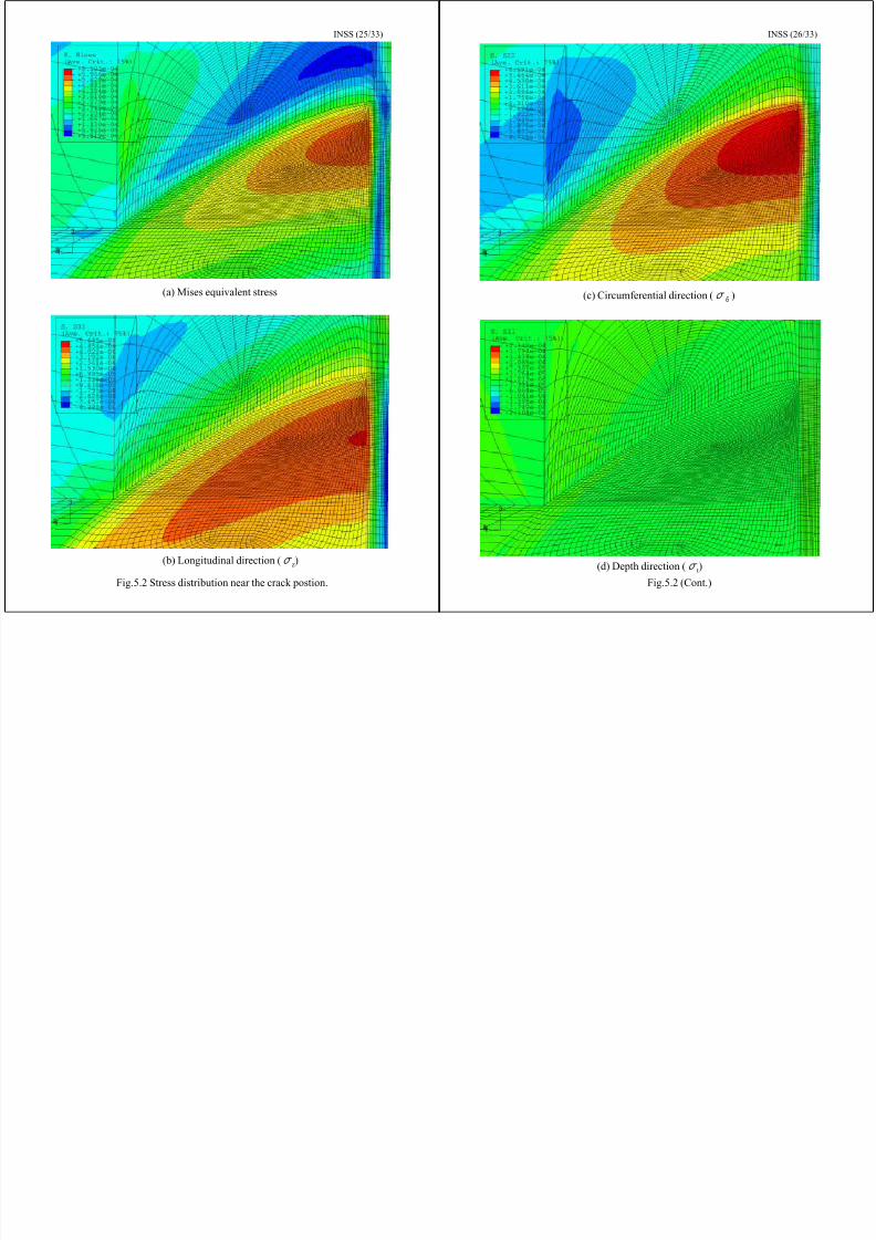
7/31/2019 Nea Study of Thermal Fatigue
http://slidepdf.com/reader/full/nea-study-of-thermal-fatigue 67/147
(a) Mises equivalent stress
(b) Longitudinal direction ( ( z)
Fig.5.2 Stress distribution near the crack postion.
(c) Circumferential direction ( ( ) )
(d) Depth direction ( ( t)
Fig.5.2 (Cont.)
(INSS) 19/33
INSS (27/33)
400
600
800
M P a
Sr Sz
205
210
215
220
m
(INSS) 20/33
35
40
45
M P a m
0 . 5
1.52.53.5
:+(mm): /8=0.5Circumferential crack < = 201 mm
INSS (28/33)
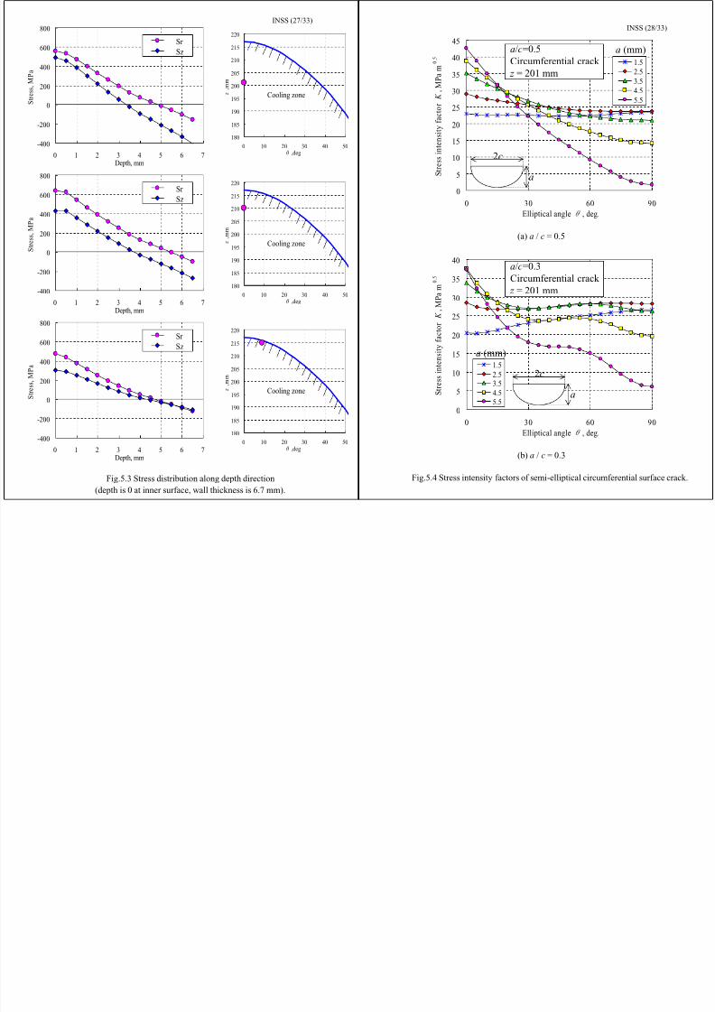
7/31/2019 Nea Study of Thermal Fatigue
http://slidepdf.com/reader/full/nea-study-of-thermal-fatigue 68/147
-400
-200
0
200
0 1 2 3 4 5 6 7Depth, mm
S t r e s s ,
180
185
190
195
200
0 10 20 30 40 502 ,deg
< , m
Cooling zone
180
185
190
195
200
205
210
215
220
0 10 20 30 40 502 ,deg
< , m
m
Cooling zone
-400
-200
0
200
400
600
800
0 1 2 3 4 5 6 7Depth, mm
S t r e s s , M P a
Sr Sz
180
185
190
195
200
205
210
215
220
0 10 20 30 40 502 ,deg
< , m
m
Cooling zone
-400
-200
0
200
400
600
800
0 1 2 3 4 5 6 7Depth, mm
S t r e s s , M P a
Sr Sz
Fig.5.3 Stress distribution along depth direction(depth is 0 at inner surface, wall thickness is 6.7 mm).
0
5
10
15
20
25
30
0 30 60 90Elliptical angle " , deg.
S t r e s s i n t e n s i t y f a c t o r #
, M 3.54.5
5.5
28
:
(a) : / 8 = 0.5
0
5
10
15
20
25
30
35
40
0 30 60 90Elliptical angle " , deg.
S t r e s s i n t e n s i t y f a c t o r #
, M P a m
0 . 5
1.52.53.54.55.5
:+(mm)
: /8=0.3
Circumferential crack < = 201 mm
28
:
(b) : / 8 = 0.3
Fig.5.4 Stress intensity factors of semi-elliptical circumferential surface crack.
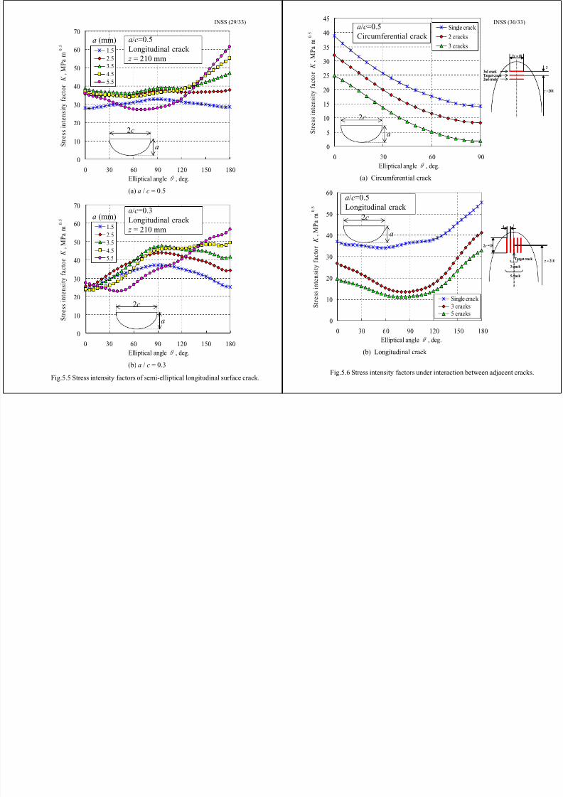
7/31/2019 Nea Study of Thermal Fatigue
http://slidepdf.com/reader/full/nea-study-of-thermal-fatigue 69/147
(INSS) 23/33
INSS (31/33)
(INSS) 24/33
INSS (32/33)
Start of crack growth prediction
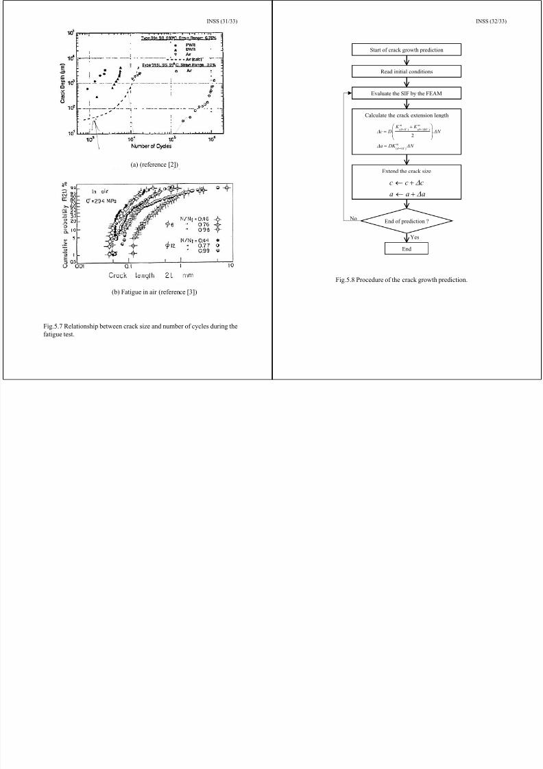
7/31/2019 Nea Study of Thermal Fatigue
http://slidepdf.com/reader/full/nea-study-of-thermal-fatigue 70/147
(a) From reference [2](a) (reference [2])
(b) Fatigue in air (reference [3])
Fig.5.7 Relationship between crack size and number of cycles during thefatigue test.
Calculate the crack extension length
Extend the crack size
8 8 8
: : :
,
,
3 )3 )
No
( = 0 ) ( = 180 )
( =90 )
2
7 7
7
# # 8 9 6
: 9# 6
* *
*
, ,
, ,
- .)/ 0'/ 01 2
'
! !
!
Evaluate the SIF by the FEAM
End of prediction ?
End
Read initial conditions
Yes
Fig.5.8 Procedure of the crack growth prediction.
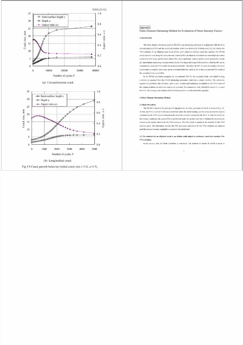
7/31/2019 Nea Study of Thermal Fatigue
http://slidepdf.com/reader/full/nea-study-of-thermal-fatigue 71/147
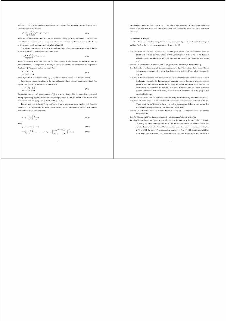
7/31/2019 Nea Study of Thermal Fatigue
http://slidepdf.com/reader/full/nea-study-of-thermal-fatigue 72/147
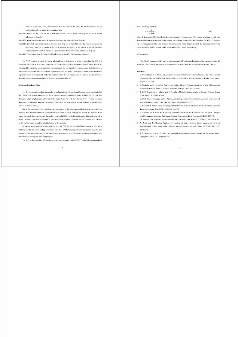
7/31/2019 Nea Study of Thermal Fatigue
http://slidepdf.com/reader/full/nea-study-of-thermal-fatigue 73/147
Crack
Finite elementanalyses
VNA solutionFEAM subroutine
Start
Determine stress interpolation points (IPs)
Step (1) Read crack data (shape, location, inclination etc.) Crack data
Step (2) Step (0)
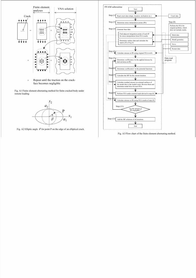
7/31/2019 Nea Study of Thermal Fatigue
http://slidepdf.com/reader/full/nea-study-of-thermal-fatigue 74/147
= +
++
+ Repeat until the traction on the crack-face becomes negligible
Fig. A1 Finite element alternating method for finite cracked body under remote loading.
"
P x 1a 1
x 2a 2
Fig. A2 Elliptic angle ) for point P on the edge of an elliptical crack.
Stress
Mesh data
Model geometry
Restart data
Calculate stresses at IPs using original FEA results
Determine coefficients A in the applied stresses byderived stress at IPs
Determine coefficients C in the potential functions
Calculate the SIF for the current iteration
Calculate residual stresses on external surfaces of the model due to the loaded crack. Reverse them and determine nodal force for next FEA.
Perform FEA under external loads derived in step (8)
Calculate stresses at IPs using FEA results of step (9)
Are the stresses atIPs negligible ?
Step (4)
Step (5)
Step (6)
Step (7)
Step (8)
Step (9)
Step (10)
Step (11)
Data read program
Perform the FEA for
original problem, whichdose not include cracks.Generate base data
Find adjacent integration points of each IPfor stress interpolation from FEA results
Determine surface data and calculate thematrix [ P ] of Eq.(3)
Add the SIF solutions of all iterations
End
Step (3)
Step (12)
Fig. A3 Flow chart of the finite element alternating method.
Crack front
x 2Interpolation points t = 10 a
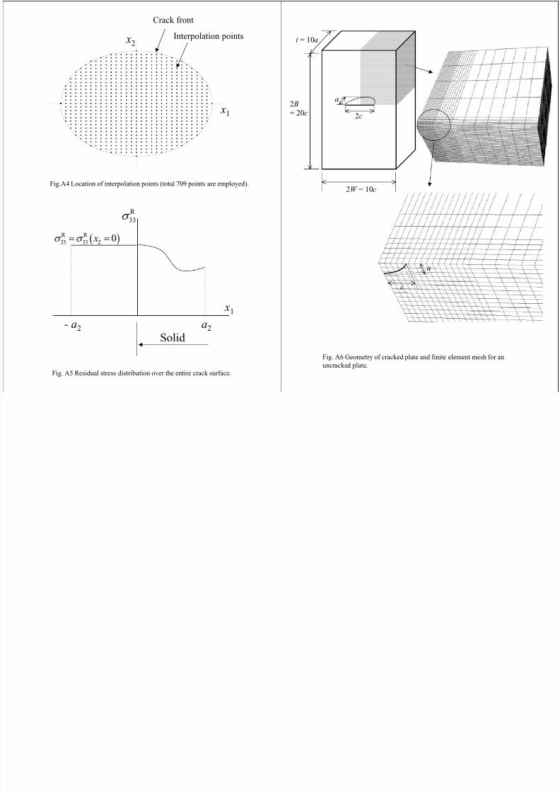
7/31/2019 Nea Study of Thermal Fatigue
http://slidepdf.com/reader/full/nea-study-of-thermal-fatigue 75/147
x 1
Fig.A4 Location of interpolation points (total 709 points are employed).
x 1
a 2- a 2
R
334 " #R R
33 33 2 0 x4 4 ' '
Solid
Fig. A5 Residual stress distribution over the entire crack surface.
2W = 10 c
c
a
c
2c
a2 B= 20
Fig. A6 Geometry of cracked plate and finite element mesh for anuncracked plate.
0 80
0.85
0.90
0.95
n s i t y
f a c t o r
F 1
1I
o
K F
a4 &
'
a /c = 0.5t /a = 10
B /c = 10W /c = 5
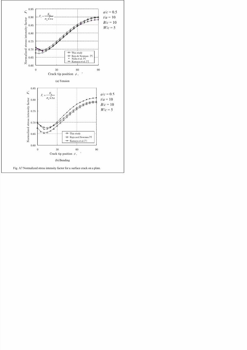
7/31/2019 Nea Study of Thermal Fatigue
http://slidepdf.com/reader/full/nea-study-of-thermal-fatigue 76/147
0.60
0.65
0.70
0.75
0.80
0 30 60 90Crack tip position #
$ , %
N o r m a
l i z e d s t r e s s
i n t e n
This studyRaju & Newman ! [*]Noda et al. [*]Kamaya et al. [*]7
89
(a) Tension
a /c = 0.5t /a = 10
B /c = 10W /c = 5
0.60
0.65
0.70
0.75
0.80
0.85
0 30 60 90Crack tip position #
$ , %
N o r m a
l i z e d
s t r e s s
i n t e n s i t y
f a c t o r
F 1
This studyRaju and Newman [*]Kamaya et al. [*]
1
I
o
K F
a4 &
'
9
7
(b) Bending
Fig. A7 Normalized stress intensity factor for a surface crack on a plate.
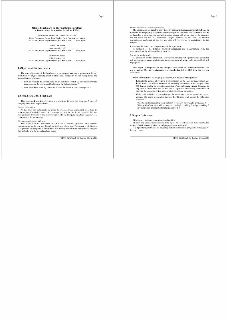
7/31/2019 Nea Study of Thermal Fatigue
http://slidepdf.com/reader/full/nea-study-of-thermal-fatigue 77/147
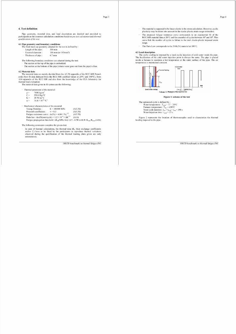
7/31/2019 Nea Study of Thermal Fatigue
http://slidepdf.com/reader/full/nea-study-of-thermal-fatigue 78/147
Page 5 Page 6
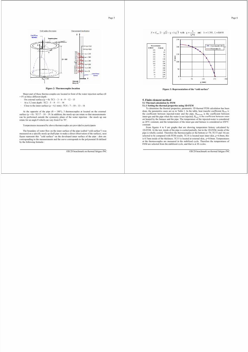
7/31/2019 Nea Study of Thermal Fatigue
http://slidepdf.com/reader/full/nea-study-of-thermal-fatigue 79/147
Figure 2: Thermocouples location
Major part of these thermo-couples are located in front of the water injection surface (
= 0°) at three different depth :On external surface ( = 0): TC1 – 3 – 6 – 9 – 12 – 15At a 3.2 mm depth : TC2 – 5 – 8 – 11 – 14Close to the inner surface ( = 6,1 mm) : TC4 – 7 – 10 – 13 – 16
At the opposite of the pipe ( = 180°), 3 thermocouples at located on the externalsurface ( = 0) : TC17 – 18 – 19. In addition, the mock-up can rotate so that measurementscan be performed outside the symmetry plane of the water injection : the mock up canrotate for an angle which can vary from 0 to 70°.
Temperatures measured by above thermocouples are provided to participants
The boundary of water flow on the inner surface of the pipe (called “cold surface”) wasmeasured on a specific mock up (half pipe to make a direct observation of the surface), nextfigure represent this cold surface” on the developed inner surface of the pipe : dots arecorresponding to the measurements and the curve corresponds to the polynomial fit defined
by the following formula :
OECD benchmark on thermal fatigue-JNC
Figure 3: Representation of the “cold surface”
5. Finite element method5.1 Thermal calculation by FEM5.1.1 Setting the thermal properties using 1D-FEM
To determine the thermal properties, parametric 1D thermal FEM calculation has beendone, the parametric cases are as in Table 1. In the table, heat transfer coefficient H water isthe coefficient between injected-water and the pipe, H inner-gas is the coefficient betweeninner-gas and the pipe when the water is not injected, H outer is the coefficient between outer air heated by the furnace and the pipe. The temperature of the injected-water is consideredas 20°C constant, and the temperature of the inner-gas and furnace is considered as 650°Cconstant.
From figures 4 to 9 are graphs that are showing temperature history calculated by1D-FEM. At the test, inside of the pipe is cooled partially, but in the 1D-FEM, inside of the pipe is wholly cooled. Therefore the thermocouples at the bottom (z=70, TC15 and 16) areselected to be compared with FEM results. TC16 is located near inner skin, =6.0mm, thisis 0.7mm inside of the thickness. TC15 is located at external skin, =0.0mm. Temperaturesat the thermocouples are measured in the stabilized cycle. Therefore the temperatures of FEM are selected from the stabilized cycle, and that is at 10 cycles.
OECD benchmark on thermal fatigue-JNC
Page 7
Figures 4 and 5 show that H outer is quite higher than 5W/m 2/°C. The capability of furnace is not sure in this benchmark, so H outer was decided from parametric FEM, and
Page 8
Table 1: Parametric cases for 1D thermal FEMcase 1-1 case 1-2 case 1-3 case 1-4 case 1-5 case 1-6 case 1-7
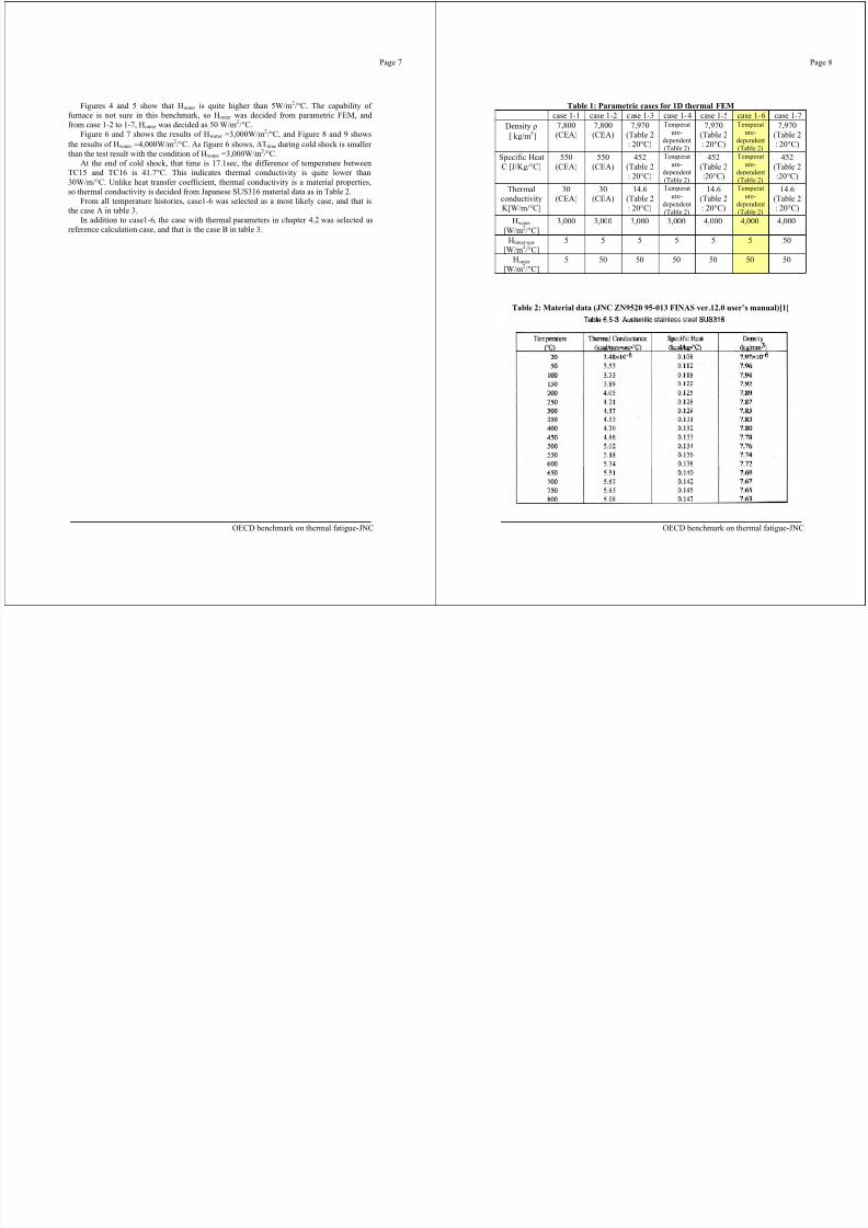
7/31/2019 Nea Study of Thermal Fatigue
http://slidepdf.com/reader/full/nea-study-of-thermal-fatigue 80/147
p
from case 1-2 to 1-7, H outer was decided as 50 W/m2
/°C.Figure 6 and 7 shows the results of H water =3,000W/m 2/°C, and Figure 8 and 9 showsthe results of H water =4,000W/m 2/°C. As figure 6 shows, Ttime during cold shock is smaller than the test result with the condition of H water =3,000W/m 2/°C.
At the end of cold shock, that time is 17.1sec, the difference of temperature betweenTC15 and TC16 is 41.7°C. This indicates thermal conductivity is quite lower than30W/m/°C. Unlike heat transfer coefficient, thermal conductivity is a material properties,so thermal conductivity is decided from Japanese SUS316 material data as in Table 2.
From all temperature histories, case1-6 was selected as a most likely case, and that isthe case A in table 3.
In addition to case1-6, the case with thermal parameters in chapter 4.2 was selected asreference calculation case, and that is the case B in table 3.
OECD benchmark on thermal fatigue-JNC
Densitykg/m 3]
7,800(CEA) 7,800(CEA) 7,970(Table 2: 20°C)
Temperature-dependent(Table 2)
7,970(Table 2: 20°C)
Temperature-dependent(Table 2)
7,970(Table 2: 20°C)
Specific HeatC [J/Kg/°C]
550(CEA)
550(CEA)
452(Table 2: 20°C)
Temperature-
dependent(Table 2)
452(Table 2:20°C)
Temperature-
dependent(Table 2)
452(Table 2:20°C)
ThermalconductivityK[W/m/°C]
30(CEA)
30(CEA)
14.6(Table 2: 20°C)
Temperature-
dependent(Table 2)
14.6(Table 2: 20°C)
Temperature-
dependent(Table 2)
14.6(Table 2: 20°C)
Hwater
[W/m2
/°C]
3,000 3,000 3,000 3,000 4,000 4,000 4,000
H inner-gas
[W/m 2/°C]5 5 5 5 5 5 50
Houter
[W/m 2/°C]5 50 50 50 50 50 50
Table 2: Material data (JNC ZN9520 95-013 FINAS ver.12.0 user’s manual)[1]
OECD benchmark on thermal fatigue-JNC
Page 9
Table 3: Selected cases from 1D thermal FEMcase A case B
Page 10
300 TC16-0°
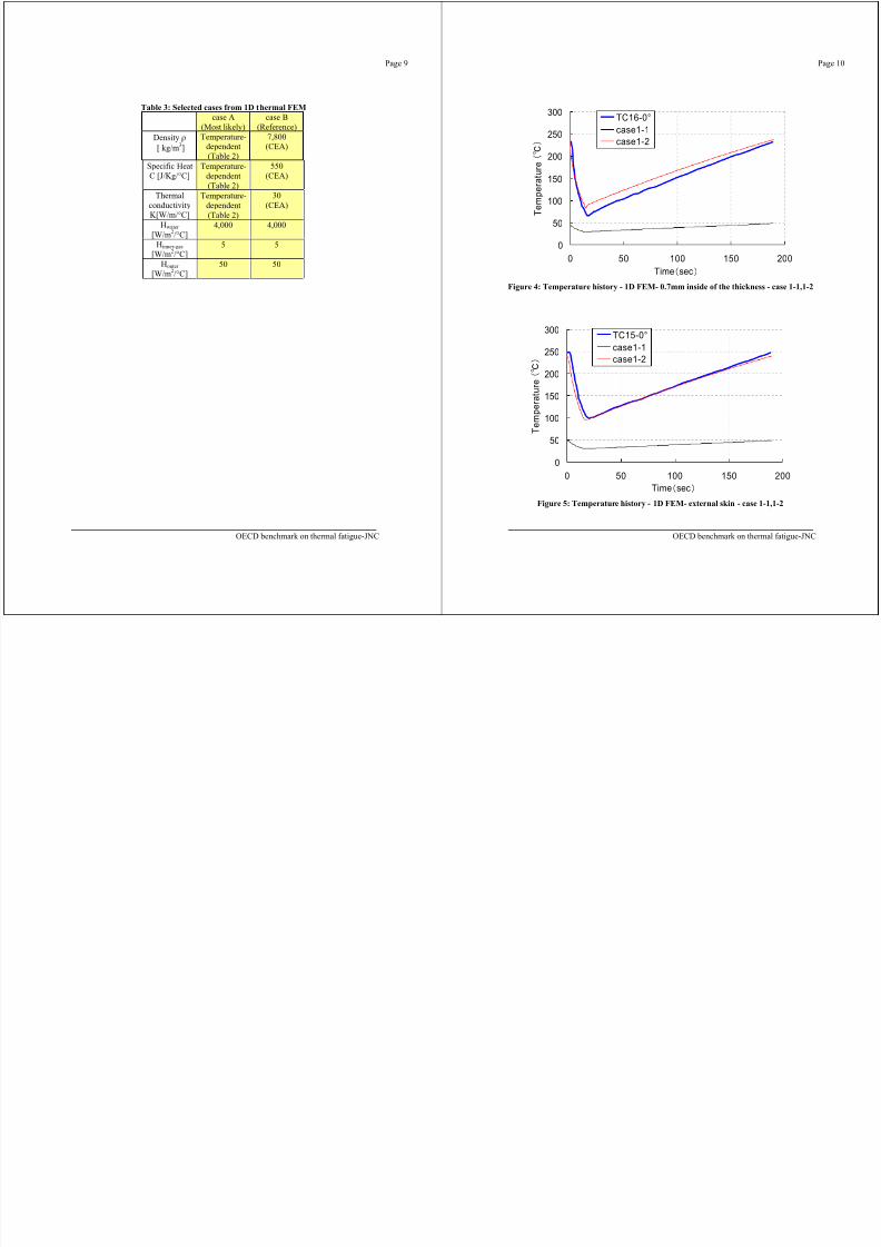
7/31/2019 Nea Study of Thermal Fatigue
http://slidepdf.com/reader/full/nea-study-of-thermal-fatigue 81/147
(Most likely) (Reference)Densitykg/m 3]
Temperature-dependent(Table 2)
7,800(CEA)
Specific HeatC [J/Kg/°C]
Temperature-dependent(Table 2)
550(CEA)
ThermalconductivityK[W/m/°C]
Temperature-dependent(Table 2)
30(CEA)
Hwater
[W/m2
/°C]
4,000 4,000
H inner-gas
[W/m 2/°C]5 5
Houter
[W/m 2/°C]50 50
OECD benchmark on thermal fatigue-JNC
0
50
100
150
200
250
0 50 100 150 200Time sec
T e m p e r a
t u r e
case1-1case1-2
Figure 4: Temperature history - 1D FEM- 0.7mm inside of the thickness - case 1-1,1-2
0
50
100
150
200
250
300
0 50 100 150 200Time sec
T e m p e r a
t u r e
TC15-0°
case1-1case1-2
Figure 5: Temperature history - 1D FEM- external skin - case 1-1,1-2
OECD benchmark on thermal fatigue-JNC
Page 11
300TC16-0°
Page 12
300TC16-0°
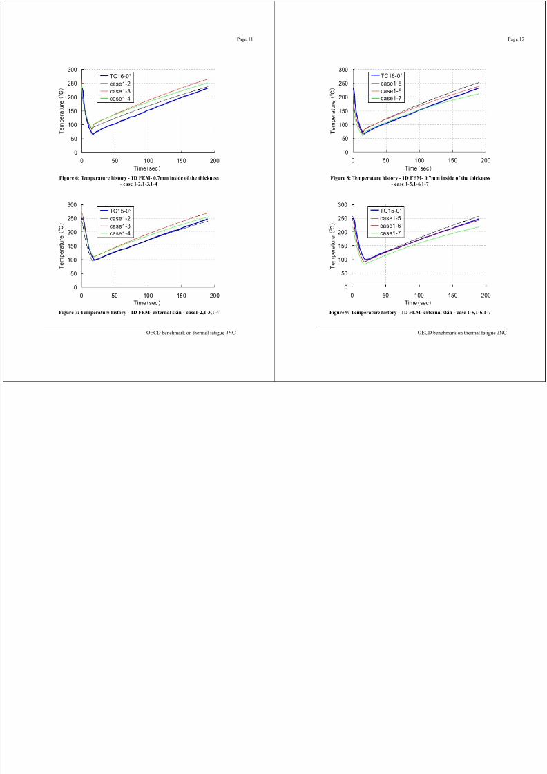
7/31/2019 Nea Study of Thermal Fatigue
http://slidepdf.com/reader/full/nea-study-of-thermal-fatigue 82/147
0
50
100
150
200
250
0 50 100 150 200Time sec
T e m p e r a
t u r e
TC16 0case1-2case1-3case1-4
Figure 6: Temperature history - 1D FEM- 0.7mm inside of the thickness- case 1-2,1-3,1-4
0
50
100
150
200
250
300
0 50 100 150 200Time sec
T e m p e r a
t u r e
TC15-0°case1-2case1-3case1-4
Figure 7: Temperature history - 1D FEM- external skin - case1-2,1-3,1-4
OECD benchmark on thermal fatigue-JNC
0
50
100
150
200
250
0 50 100 150 200Time sec
T e m p e r a
t u r e
TC16 0case1-5case1-6case1-7
Figure 8: Temperature history - 1D FEM- 0.7mm inside of the thickness- case 1-5,1-6,1-7
0
50
100
150
200
250
300
0 50 100 150 200Time sec
T e m p e r a
t u r e
TC15-0°case1-5case1-6case1-7
Figure 9: Temperature history - 1D FEM- external skin - case 1-5,1-6,1-7
OECD benchmark on thermal fatigue-JNC
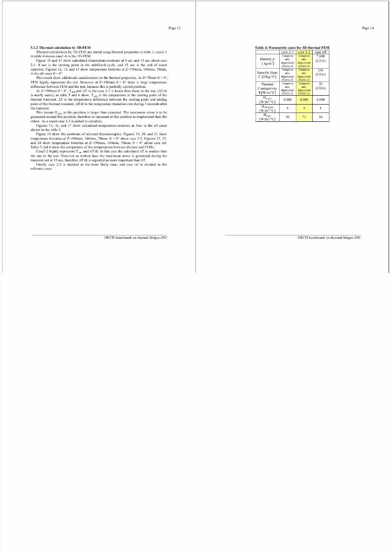
7/31/2019 Nea Study of Thermal Fatigue
http://slidepdf.com/reader/full/nea-study-of-thermal-fatigue 83/147
Page 15
Table 5: Comparison of the temperatures = 0°0.7mm inside (TC4) External skin (TC3)Z=190mm
Page 16
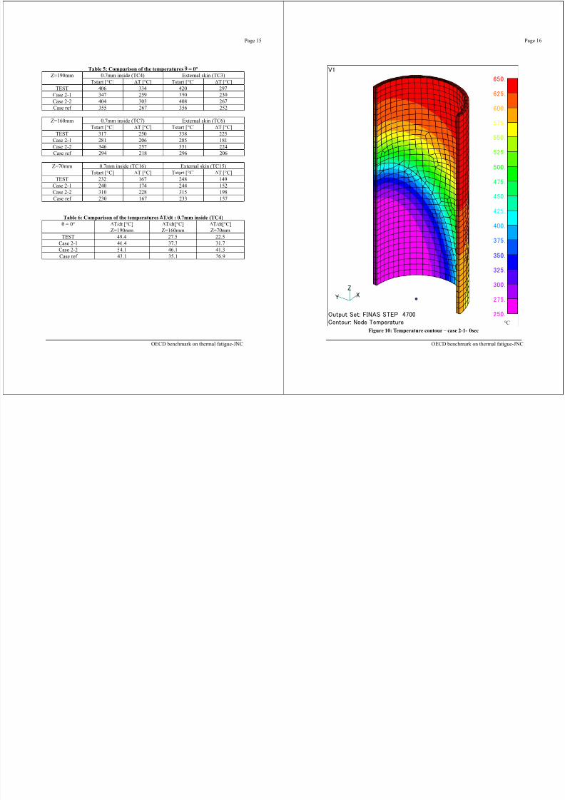
7/31/2019 Nea Study of Thermal Fatigue
http://slidepdf.com/reader/full/nea-study-of-thermal-fatigue 84/147
Tstart [°C] T [°C] Tstart [°C] T [°C]TEST 406 334 420 297Case 2-1 347 259 350 230Case 2-2 404 303 408 267Case ref 355 267 356 252
0.7mm inside (TC7) External skin (TC6)Z=160mmTstart [°C] T [°C] Tstart [°C] T [°C]
TEST 317 250 338 225Case 2-1 281 206 285 181Case 2-2 346 257 351 224
Case ref 294 218 296 206
0.7mm inside (TC16) External skin (TC15)Z=70mmTstart [°C] T [°C] Tstart [°C] T [°C]
TEST 232 167 248 149Case 2-1 240 174 244 152Case 2-2 310 228 315 198Case ref 230 167 233 157
Table 6: Comparison of the temperatures T/dt : 0.7mm inside (TC4)= 0° T/dt [°C]
Z=190mmT/dt[°C]
Z=160mmT/dt[°C]
Z=70mmTEST 49.4 27.5 22.5
Case 2-1 46.4 37.3 31.7Case 2-2 54.1 46.1 41.3Case ref 43.1 35.1 26.9
OECD benchmark on thermal fatigue-JNC
°CFigure 10: Temperature contour – case 2-1- 0sec
OECD benchmark on thermal fatigue-JNC
Page 17 Page 18
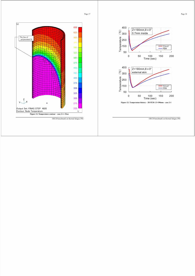
7/31/2019 Nea Study of Thermal Fatigue
http://slidepdf.com/reader/full/nea-study-of-thermal-fatigue 85/147
The line of polynominal fit
°CFigure 11: Temperature contour – case 2-1- 15sec
OECD benchmark on thermal fatigue-JNC
50
15 0
25 0
35 045 0
0 50 100 150 200Time (sec)
T e m p e r a
t u r e
TC4-0°FEM
50
15 0
25 0
35 0
45 0
0 50 100 150 200Time (sec)
T e m p e r a
t u r e
TC3-0°FEM
Z=190mm, 0°0.7mm inside
Z=190mm, 0°external skin
Figure 12: Temperature history - 3D FEM- Z=190mm - case 2-1
OECD benchmark on thermal fatigue-JNC
Page 19
450
Page 20
45 0
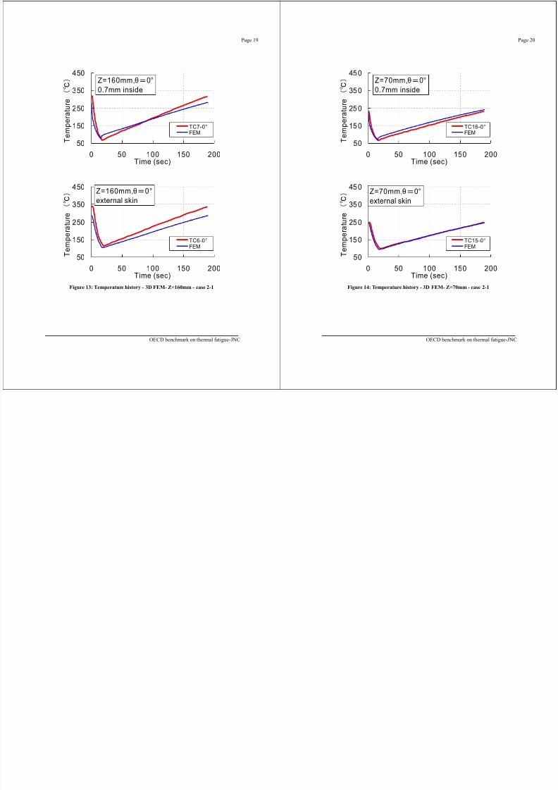
7/31/2019 Nea Study of Thermal Fatigue
http://slidepdf.com/reader/full/nea-study-of-thermal-fatigue 86/147
50
150
250
350
0 50 100 150 200Time (sec)
T e m p e r a
t u r e
TC7-0°FEM
50
150
250
350
450
0 50 100 150 200Time (sec)
T e m p e r a
t u r e
TC6-0°FEM
Z=160mm, 0°0.7mm inside
Z=160mm, 0°external skin
Figure 13: Temperature history - 3D FEM- Z=160mm - case 2-1
OECD benchmark on thermal fatigue-JNC
50
15 0
25 0
35 0
0 50 100 150 200Time (sec)
T e m p e r a
t u r e
TC16-0°FEM
50
15 0
25 0
35 0
45 0
0 50 100 150 200Time (sec)
T e m p e r a
t u r e
TC15-0°FEM
Z=70mm, 0°0.7mm inside
Z=70mm, 0°external skin
Figure 14: Temperature history - 3D FEM- Z=70mm - case 2-1
OECD benchmark on thermal fatigue-JNC
Page 21 Page 22
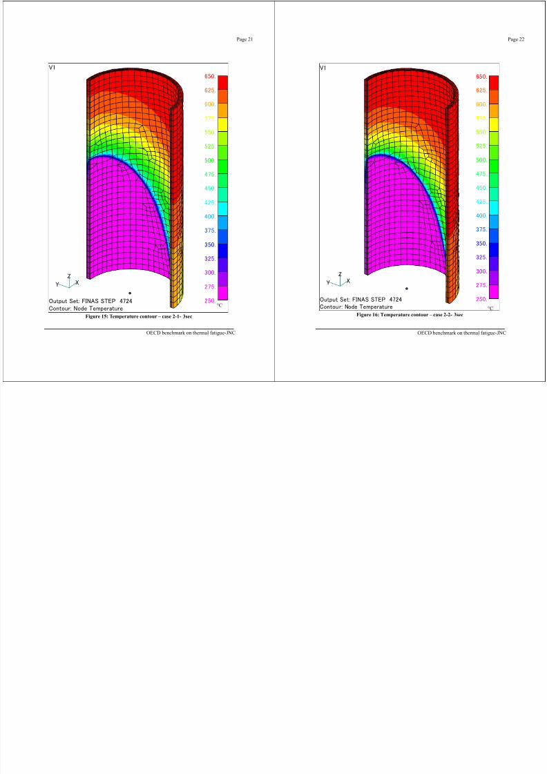
7/31/2019 Nea Study of Thermal Fatigue
http://slidepdf.com/reader/full/nea-study-of-thermal-fatigue 87/147
°C
Figure 15: Temperature contour – case 2-1- 3sec
OECD benchmark on thermal fatigue-JNC
°CFigure 16: Temperature contour – case 2-2- 3sec
OECD benchmark on thermal fatigue-JNC
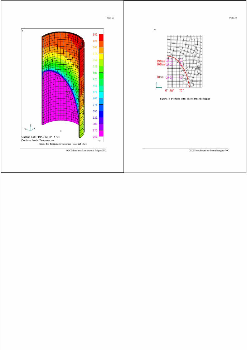
7/31/2019 Nea Study of Thermal Fatigue
http://slidepdf.com/reader/full/nea-study-of-thermal-fatigue 88/147
Page 25
45 0 Z=190mm, 0°
Page 26
450
Z 160 0°
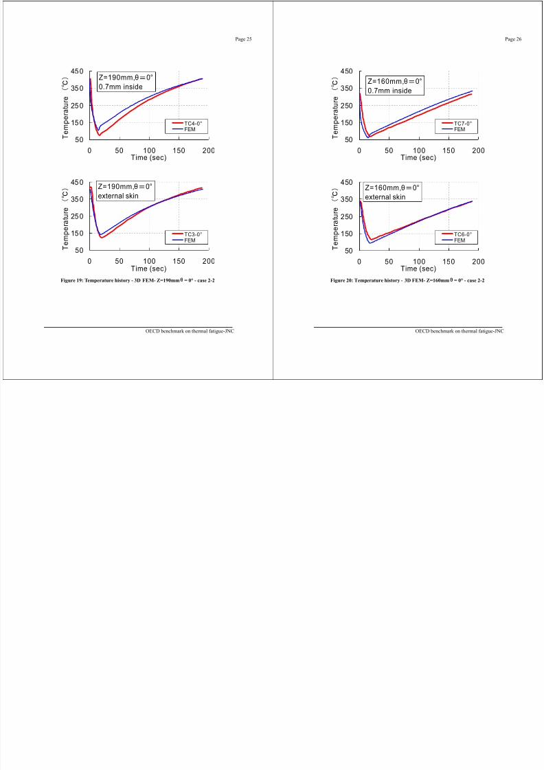
7/31/2019 Nea Study of Thermal Fatigue
http://slidepdf.com/reader/full/nea-study-of-thermal-fatigue 89/147
50
15 0
25 0
35 0
0 50 100 150 200Time (sec)
T e m p e r a
t u r e
TC4-0°FEM
50
15 0
25 0
35 0
45 0
0 50 100 150 200Time (sec)
T e m p e r a t u r e
TC3-0°FEM
0.7mm inside
Z=190mm, 0°external skin
Figure 19: Temperature history - 3D FEM- Z=190mm = 0° - case 2-2
OECD benchmark on thermal fatigue-JNC
50
150
250
350
0 50 100 150 200Time (sec)
T e m p e r a
t u r e
TC7-0°FEM
50
150
250
350
450
0 50 100 150 200Time (sec)
T e m p e r a t u r e
TC6-0°FEM
Z=160mm, 0°0.7mm inside
Z=160mm, 0°external skin
Figure 20: Temperature history - 3D FEM- Z=160mm = 0° - case 2-2
OECD benchmark on thermal fatigue-JNC
Page 27
45 0
Z=70mm 0°
Page 28
450 Z=190mm, 0°
d
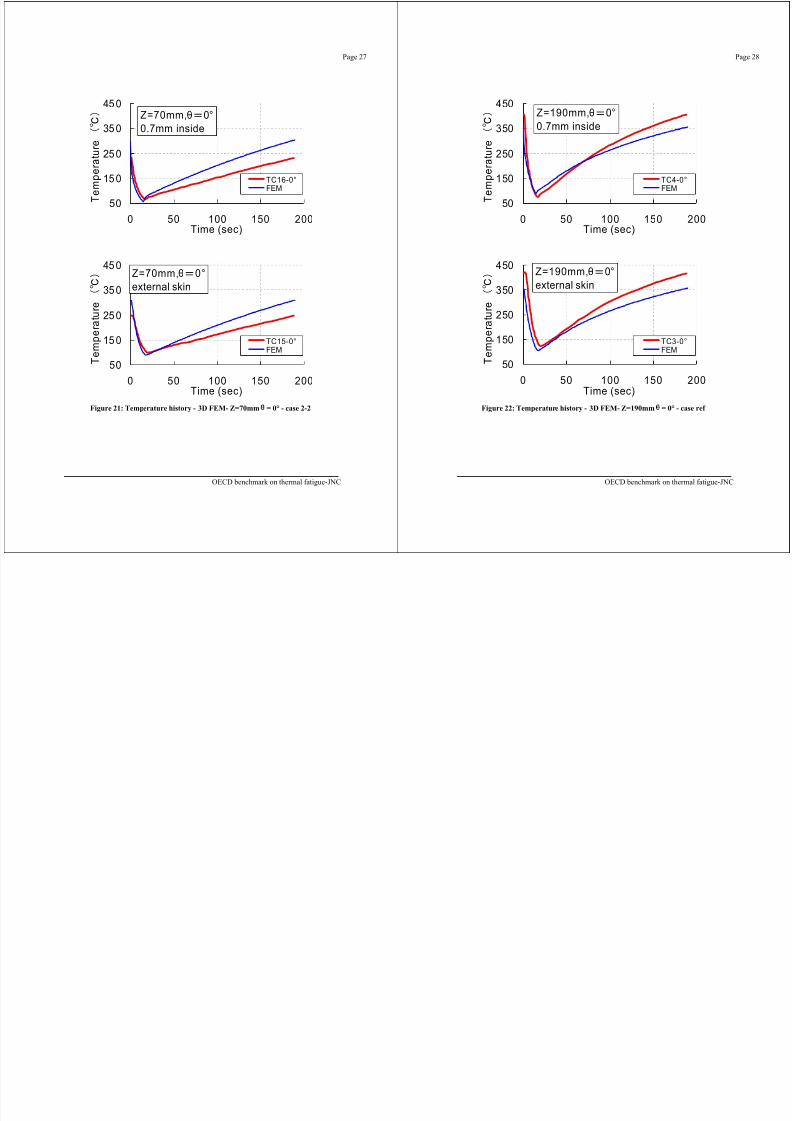
7/31/2019 Nea Study of Thermal Fatigue
http://slidepdf.com/reader/full/nea-study-of-thermal-fatigue 90/147
50
15 0
25 0
35 0
0 50 100 150 200Time (sec)
T e m p e r a
t u r e
TC16-0°FEM
50
15 0
25 0
35 0
45 0
0 50 100 150 200Time (sec)
T e m p e r a t u r e
TC15-0°FEM
Z=70mm, 0°0.7mm inside
Z=70mm, 0°external skin
Figure 21: Temperature history - 3D FEM- Z=70mm = 0° - case 2-2
OECD benchmark on thermal fatigue-JNC
50
150
250
350
0 50 100 150 200Time (sec)
T e m p e r a
t u r e
TC4-0°FEM
50
150
250
350
450
0 50 100 150 200Time (sec)
T e m p e r a t u r e
TC3-0°FEM
0.7mm inside
Z=190mm, 0°external skin
Figure 22: Temperature history - 3D FEM- Z=190mm = 0° - case ref
OECD benchmark on thermal fatigue-JNC
Page 29
45 0
Z=160mm 0°0 7 i id
Page 30
45 0
Z=70mm 0°0 7 i id
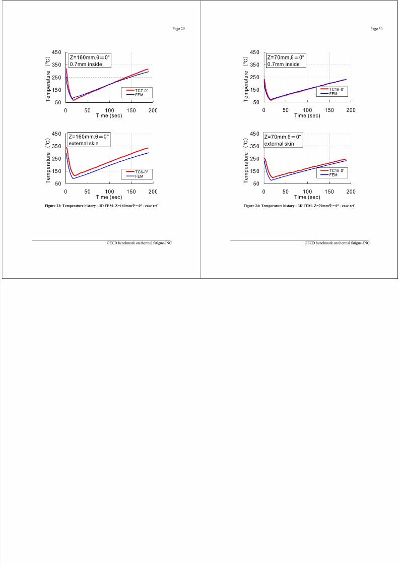
7/31/2019 Nea Study of Thermal Fatigue
http://slidepdf.com/reader/full/nea-study-of-thermal-fatigue 91/147
50
15 0
25 0
35 0
0 50 100 150 200Time (sec)
T e m p e r a
t u r e
TC7-0°FEM
50
15 0
25 0
35 0
45 0
0 50 100 150 200Time (sec)
T e m p e r a t u r e
TC6-0°FEM
Z=160mm, 00.7mm inside
Z=160mm, 0°external skin
Figure 23: Temperature history - 3D FEM- Z=160mm = 0° - case ref
OECD benchmark on thermal fatigue-JNC
50
15 0
25 0
35 0
0 50 100 150 200Time (sec)
T e m p e r a
t u r e
TC16-0°FEM
50
15 0
25 0
35 0
45 0
0 50 100 150 200Time (sec)
T e m p e r a t u r e
TC15-0°FEM
Z=70mm, 00.7mm inside
Z=70mm, 0°external skin
Figure 24: Temperature history - 3D FEM- Z=70mm = 0° - case ref
OECD benchmark on thermal fatigue-JNC
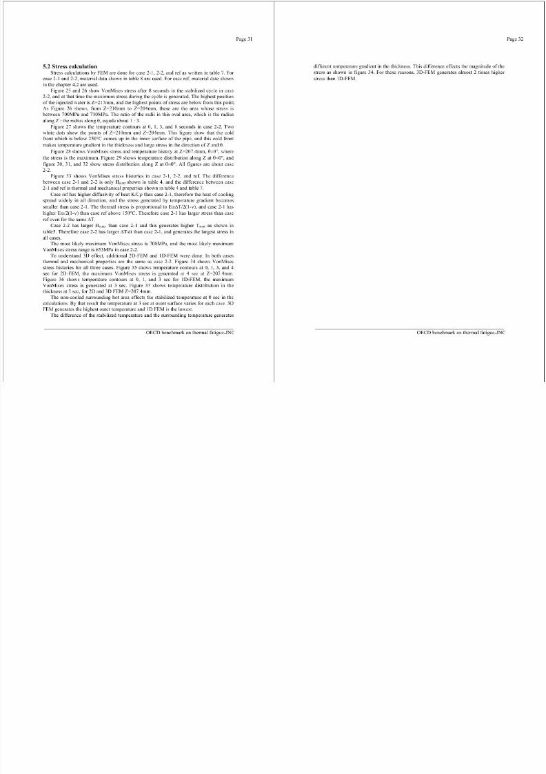
7/31/2019 Nea Study of Thermal Fatigue
http://slidepdf.com/reader/full/nea-study-of-thermal-fatigue 92/147
Page 33
Table 7: Analyses cases for 3D stress FEMcase 2-1 case 2-2 case ref
Young’s ModulusMPa]
Temperature-dependent
Temperature-dependent
186000(A3.3S)
Page 34
Table 8: Material data (JNC ZN9520 95-013 FINAS ver.12.0 user’s manual) [1]
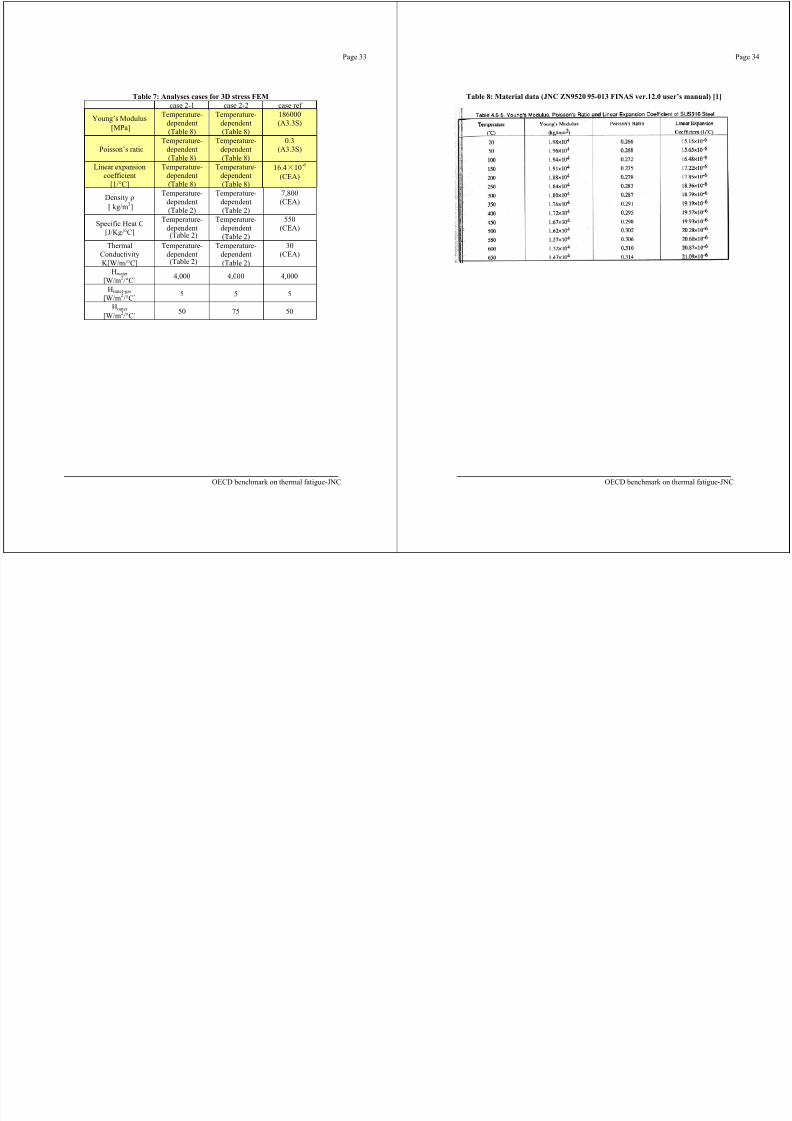
7/31/2019 Nea Study of Thermal Fatigue
http://slidepdf.com/reader/full/nea-study-of-thermal-fatigue 93/147
MPa] (Table 8) (Table 8)
Poisson’s ratioTemperature-
dependent(Table 8)
Temperature-dependent(Table 8)
0.3(A3.3S)
Linear expansioncoefficient
[1/°C]
Temperature-dependent(Table 8)
Temperature-dependent(Table 8)
16.4 10 -6
(CEA)
Densitykg/m 3]
Temperature-dependent(Table 2)
Temperature-dependent(Table 2)
7,800(CEA)
Specific Heat C[J/Kg/°C]
Temperature-dependent(Table 2)
Temperature-dependent(Table 2)
550(CEA)
ThermalConductivityK[W/m/°C]
Temperature-dependent(Table 2)
Temperature-dependent(Table 2)
30(CEA)
Hwater
[W/m 2/°C] 4,000 4,000 4,000
H inner-gas
[W/m 2/°C] 5 5 5
Houter
[W/m 2/°C] 50 75 50
OECD benchmark on thermal fatigue-JNC OECD benchmark on thermal fatigue-JNC
Page 35 Page 36
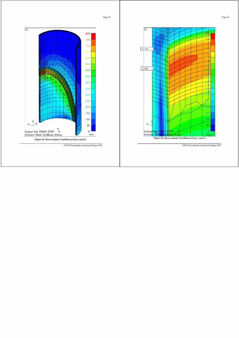
7/31/2019 Nea Study of Thermal Fatigue
http://slidepdf.com/reader/full/nea-study-of-thermal-fatigue 94/147
MPa
Figure 25: Stress contour (VonMises) at 8sec: case2-2
OECD benchmark on thermal fatigue-JNC
Z=204
Z=210
MPa
Figure 26: Stress contour (VonMises) at 8 sec: case2-2
OECD benchmark on thermal fatigue-JNC
Page 37
Time=0sec
Page 38
60 070 0
80 0
)
=0°
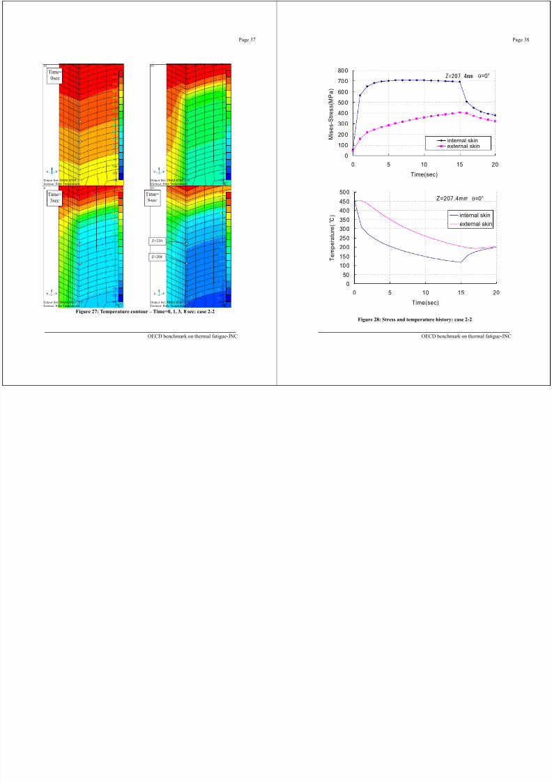
7/31/2019 Nea Study of Thermal Fatigue
http://slidepdf.com/reader/full/nea-study-of-thermal-fatigue 95/147
Time=3sec
°C
Time=8sec
Z=210
Z=204
Figure 27: Temperature contour – Time=0, 1, 3, 8 sec: case 2-2°C °C
OECD benchmark on thermal fatigue-JNC
050
10 0
15 0
20 0
25 0
30 035 0
40 0
45 0
50 0
0 5 10 15 20
Time(sec)
T e m p e r a
t u r e
( ) internal skin
external skin
Z=207.4mm =0°
0
10 0
20 0
30 0
40 0
50 0
60 0
0 5 10 15 20
Time(sec)
M i s e s - S
t r e s s
( M P a
internal skinexternal skin
Figure 28: Stress and temperature history: case 2-2
OECD benchmark on thermal fatigue-JNC
Page 39
600
700Internal skin
Page 40
700
800
Internal skin
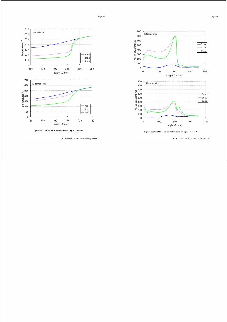
7/31/2019 Nea Study of Thermal Fatigue
http://slidepdf.com/reader/full/nea-study-of-thermal-fatigue 96/147
0
100
200
300
400
500
150 170 190 210 230 250
height -Z (mm)
t e m p e r a
t u r e
( )
0sec3sec8sec
0
100
200
300
400
500
600
700
150 170 190 210 230 250height -Z (mm)
t e m p e r a
t u r e
( )
0sec3sec8sec
External skin
Figure 29: Temperature distribution along Z: case 2-2
OECD benchmark on thermal fatigue-JNC
0
100
200
300
400
500
600
0 100 200 300 400
height -Z (mm)
M i s e s s
t r e s s
( M P a
)
0sec3sec8sec
0
10 0
20 0
30 0
40 0
50 0
60 070 0
80 0
90 0
0 100 200 300 400
height -Z (mm)
M i s e s s
t r e s s
( M P a )
0sec3sec8sec
External skin
Figure 30: VonMises stress distribution along Z : case 2-2
OECD benchmark on thermal fatigue-JNC
Page 41
600
800Internal skin
Page 42
600
800 Internal skin
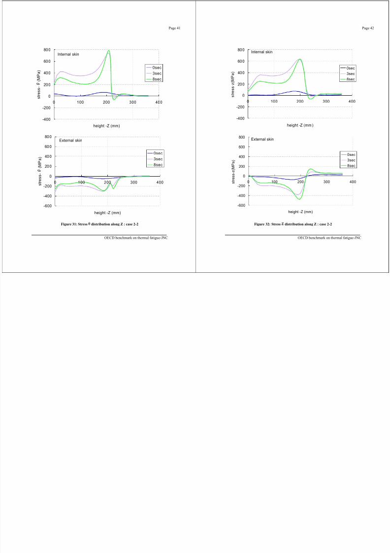
7/31/2019 Nea Study of Thermal Fatigue
http://slidepdf.com/reader/full/nea-study-of-thermal-fatigue 97/147
-400
-200
0
200
400
0 100 200 300 400
height -Z (mm)
s t r e s s -
( M P a
)0sec3sec8sec
-600
-400
-200
0
200
400
600
800
0 100 200 300 400
height -Z (mm)
s t r e s s -
( M P a )
0sec3sec8sec
External skin
Figure 31: Stress distribution along Z : case 2-2
OECD benchmark on thermal fatigue-JNC
-400
-200
0
200
400
0 100 200 300 400
height -Z (mm )
s t r e s s - z
( M P a
)0sec3sec8sec
-600
-400
-200
0
200
400
600
800
0 100 200 300 400
height -Z (mm)
s t r e s s - z
( M P a
)0sec3sec8sec
External skin
Figure 32: Stress distribution along Z : case 2-2
OECD benchmark on thermal fatigue-JNC
Page 43
700
800
)
Page 44
3D (2-2)2D (2-2)1D (2-2)
2D,3D:Z=207.4mm=0°
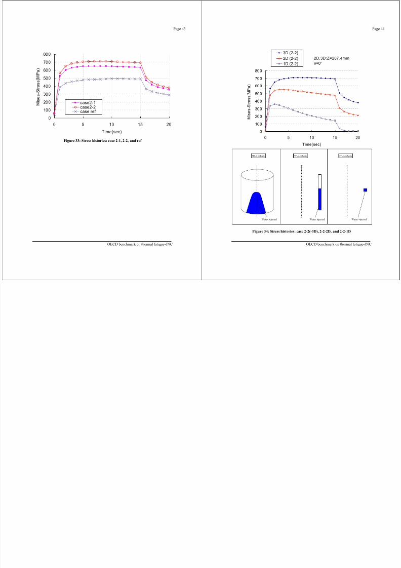
7/31/2019 Nea Study of Thermal Fatigue
http://slidepdf.com/reader/full/nea-study-of-thermal-fatigue 98/147
0100
200
300
400
500
600
0 5 10 15 20
Time(sec)
M i s e s - S
t r e s s
( M P a
)
case2-1case2-2case ref
Figure 33: Stress histories: case 2-1, 2-2, and ref
OECD benchmark on thermal fatigue-JNC
0
100
200300
400
500
600
700
800
0 5 10 15
Time(sec)
M i s e s - S
t r e s s
( M P a
)
20
3D-Analysis 2D-Analysis 1D-Analysis
Water injected Water injected Water injected
Figure 34: Stress histories: case 2-2(-3D), 2-2-2D, and 2-2-1D
OECD benchmark on thermal fatigue-JNC
Page 45
Time=0sec
Time=1sec
Page 46
Time=0sec
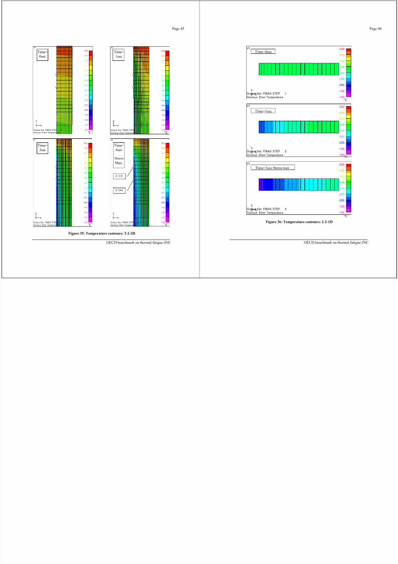
7/31/2019 Nea Study of Thermal Fatigue
http://slidepdf.com/reader/full/nea-study-of-thermal-fatigue 99/147
°C °C
Time=3sec
Z=204
Z=210
Time=4sec
StressMax.
°C °C
Figure 35: Temperature contours: 2-2-2D
OECD benchmark on thermal fatigue-JNC
°C
Time=1sec
°C
Time=3sec Stress max.
°C
Figure 36: Temperature contours: 2-2-1D
OECD benchmark on thermal fatigue-JNC
Page 47
350400
450
)
Page 48
5.3 Estimation of the crack initiation5.3.1 Estimation of the total strain range
Total strain range in case 2-2 was estimated. As Figure 38 shows, the maximum and theminimum stresses are generated at 8 and 0 second. Equivalent stress range |x=0 is 653MPa.
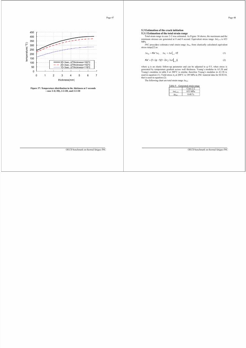
7/31/2019 Nea Study of Thermal Fatigue
http://slidepdf.com/reader/full/nea-study-of-thermal-fatigue 100/147
050
100
150
200
250
300
0 1 2 3 4 5 6 7
thickness(mm)
t e m p e r a
t u r e
(
)
3D-3sec, Tthickness=1622D-3sec, Tthickness=152
1D-3sec, Tthickness=116
Figure 37: Temperature distribution in the thickness at 3 seconds: case 2-2(-3D), 2-2-2D, and 2-2-1D
OECD benchmark on thermal fatigue-JNC
JNC procedure estimates total strain range tot from elastically calculated equivalentstress range[2] as
, 0'tot e e x
Ke E / (1)
0' {1 ( 1)(1 2 / )}y x
Ke q (2)
where q is an elastic follow-up parameter and can be adjusted to q=5/3, when stress isgenerated by temperature gradient across wall thickness. Young’s modulus in A3.3S andYoung’s modulus in table 8 at 200°C is similar, therefore Young’s modulus in A3.3S isused in equation (1). Yield stress y at 200°C is 149 MPa in JNC material data for SUS316,that is used in equation (2).
The following chart are total strain range tot.
Table 9 Generated strain rangeCase 2-2
|x=0 653 MPatot 0.48 %
OECD benchmark on thermal fatigue-JNC
Page 49
5.3.2 Fatigue curves and estimation of crack initiationThis benchmark’s fatigue resistance curve is (%) = 4.84 NR
-0.2 from A3.3S.JNC has fatigue resistance curve shown in table 11 [3]. At the starting point of the
transient the temperature is 450°C, therefore this curve at 450°C is used.In this curve, the failure is defined as the number of repetitions observed when the
Page 50
Table 11: JNC fatigue resistance curve[3]
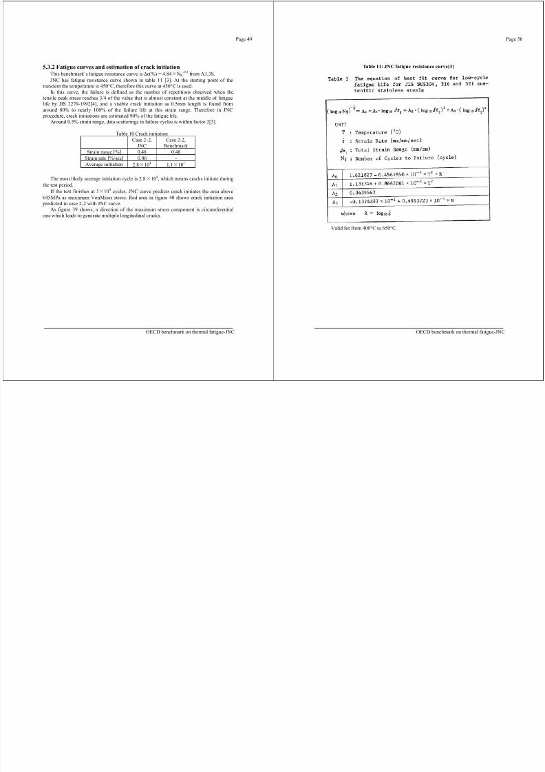
7/31/2019 Nea Study of Thermal Fatigue
http://slidepdf.com/reader/full/nea-study-of-thermal-fatigue 101/147
tensile peak stress reaches 3/4 of the value that is almost constant at the middle of fatiguelife by JIS 2279-1992[4], and a visible crack initiation as 0.5mm length is found fromaround 80% to nearly 100% of the failure life at this strain range. Therefore in JNC
procedure, crack initiations are estimated 90% of the fatigue life.Around 0.5% strain range, data scatterings in failure cycles is within factor 2[3].
Table 10 Crack initiationCase 2-2,
JNCCase 2-2,
Benchmark Strain range [%] 0.48 0.48
Strain rate [%/sec] 0.06 -Average initiation 2.8 104 1.1 105
The most likely average initiation cycle is 2.8 104, which means cracks initiate duringthe test period.
If the test finishes at 5 104 cycles. JNC curve predicts crack initiates the area above645MPa as maximum VonMises stress. Red area in figure 40 shows crack initiation area
predicted in case 2-2 with JNC curve.As figure 39 shows, a direction of the maximum stress component is circumferential
one which leads to generate multiple longitudinal cracks.
OECD benchmark on thermal fatigue-JNC
Valid for from 400°C to 650°C.
OECD benchmark on thermal fatigue-JNC
Page 51
350
400450
500
)
0sec
1sec
2sec
3sec4sec
5sec
Page 52
600700
800
)
0sec
1sec
2sec
3sec4sec
5sec
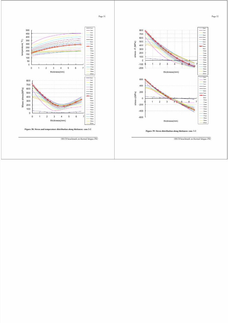
7/31/2019 Nea Study of Thermal Fatigue
http://slidepdf.com/reader/full/nea-study-of-thermal-fatigue 102/147
0
50100
150
200250
300
350
0 1 2 3 4 5 6 7
thickness(mm)
t e m p e r a
t u r e
( 6sec
7sec
8sec
9sec
10sec
11sec
12sec
13sec
14sec
15sec
16sec
17sec
18sec
19sec
20sec
0
100
200
300
400
500
600
700
800
0 1 2 3 4 5 6 7
thickness(mm)
M i s e s s
t r e s s
( M P a
)
0sec
1sec
2sec
3sec
4sec
5sec
6sec7sec
8sec
9sec
10sec
11sec
12sec
13sec
14sec
15sec
16sec
17sec
18sec
19sec
20sec
Figure 38: Stress and temperature distribution along thickness: case 2-2
OECD benchmark on thermal fatigue-JNC
-200
-100
0
100
200
300
400
500
0 1 2 3 4 5 6 7
thickness(mm)
s t r e s s -
( M P a
)6sec
7sec
8sec
9sec
10sec
11sec
12sec
13sec
14sec
15sec
16sec
17sec
18sec
19sec
20sec
-600
-400
-200
0
200
400
600
0 1 2 3 4 5 6 7
thickness(mm)
s t r e s s - z
( M P a )
0sec
1sec
2sec
3sec
4sec
5sec
6sec7sec
8sec
9sec
10sec
11sec
12sec
13sec
14sec
15sec
16sec
17sec
18sec
19sec
20sec
Figure 39: Stress distribution along thickness: case 2-2
OECD benchmark on thermal fatigue-JNC
Page 53 Page 54
5.4 Estimation of the crack propagation5.4.1 Evaluation procedure for crack propagation
In the estimation of the crack propagation, unique longitudinal semi-elliptical internalinitial crack is assumed as a fatigue initiated crack. An assumed initial crack is the onewhose depth a=0.25mm, and whose length 2c=2.5mm, c/a=5. This longer crack length isdetermined to consider coalescence and interaction of multiple cracks because in the
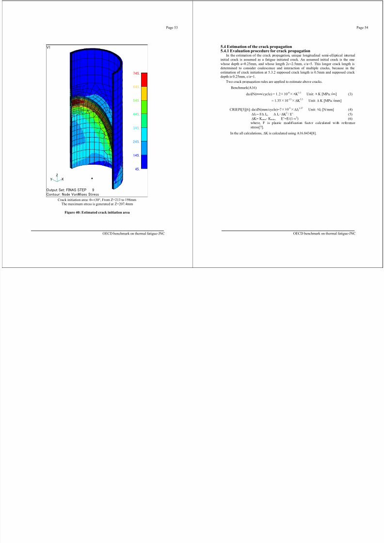
7/31/2019 Nea Study of Thermal Fatigue
http://slidepdf.com/reader/full/nea-study-of-thermal-fatigue 103/147
Crack initiation area: °, From Z=213 to 198mmThe maximum stress is generated at Z=207.4mm
Figure 40: Estimated crack initiation area
OECD benchmark on thermal fatigue-JNC
determined to consider coalescence and interaction of multiple cracks, because in theestimation of crack initiation at 5.3.2 supposed crack length is 0.5mm and supposed crack depth is 0.25mm, c/a=1.
Two crack propagation rules are applied to estimate above cracks.
Benchmark(A16):
da/dN(mm/cycle) = 1.2 10 -8 K 3.3 Unit: K [MPa. m] (3)
= 1.35 10 -13 K 3.3 Unit: K [MPa. mm]
CRIEPI[5][6]: da/dN(mm/cycle)=7 10 -5 Jf 1.37 Unit: Jf [N/mm] (4)
Jf = F Je, Je= K 2 / E’ (5)K= K max - K min , E’=E/(1- 2) (6)
where, F is plastic modification factor calculated with referencestress[7].
In the all calculations, K is calculated using A16.8434[8].
OECD benchmark on thermal fatigue-JNC
Page 55
5.4.2 Estimated Crack propagationCrack propagation is estimated for case 2-2, and the maximum K I is calculated as at 15
sec. The evaluation line is assumed as a perpendicular line from the highest stress point.The propagation until 80% is considered as a penetration and the calculations until 80%
has been done. Estimated propagation cycles are as follows. The crack length 2c at thet ti i b t 23 f b th
Page 56
4
5
6
m ]
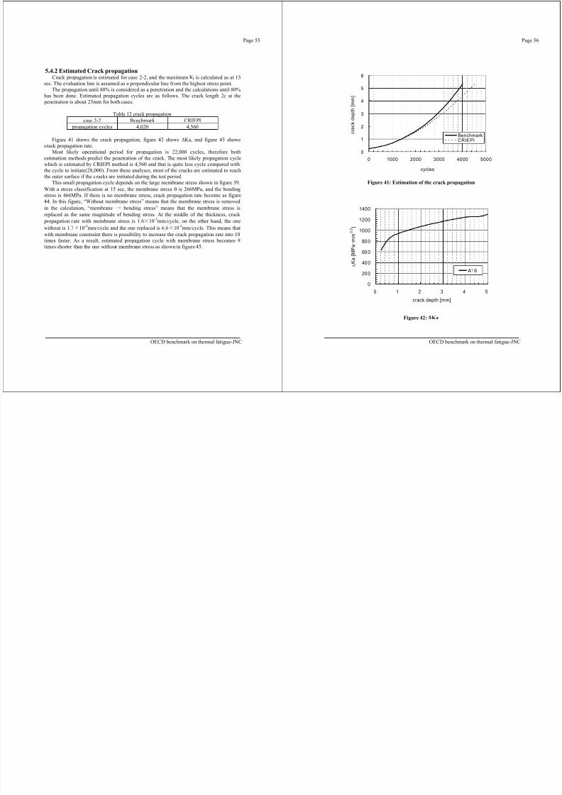
7/31/2019 Nea Study of Thermal Fatigue
http://slidepdf.com/reader/full/nea-study-of-thermal-fatigue 104/147
penetration is about 23mm for both cases.
Table 12 crack propagationcase 2-2 Benchmark CRIEPI
propagation cycles 4,020 4,560
Figure 41 shows the crack propagation, figure 42 shows Ka, and figure 43 showscrack propagation rate.
Most likely operational period for propagation is 22,000 cycles, therefore bothestimation methods predict the penetration of the crack. The most likely propagation cyclewhich is estimated by CRIEPI method is 4,560 and that is quite less cycle compared withthe cycle to initiate(28,000). From these analyses, most of the cracks are estimated to reachthe outer surface if the c racks are initiated during the test period.
This small propagation cycle depends on the large membrane stress shown in figure 39.With a stress classification at 15 sec, the membrane stress is 266MPa, and the bendingstress is 466MPa. If there is no membrane stress, crack propagation rate become as figure44. In this figure, “Without membrane stress” means that the membrane stress is removedin the calculation, “membrane bending stress” means that the membrane stress isreplaced as the same magnitude of bending stress. At the middle of the thickness, crack
propagation rate with membrane stress is 1.6 10 -3mm/cycle, on the other hand, the onewithout is 1.7 10 -4mm/cycle and the one replaced is 6.6 10 -4mm/cycle. This means thatwith membrane constraint there is possibility to increase the crack propagation rate into 10times faster. As a result, estimated propagation cycle with membrane stress becomes 9times shorter than the one without membrane stress as shown in figure 45.
OECD benchmark on thermal fatigue-JNC
0
1
2
3
4
0 1000 2000 3000 4000 5000
cycles
c r a c
k d e p
t h [ m
BenchmarkCRIEPI
Figure 41: Estimation of the crack propagation
0
200
400
600
800
1000
1200
1400
0 1 2 3 4 5
crack depth [mm]
K a
[ M P a
m m
0 . 5 ]
A16
Figure 42: Ka
OECD benchmark on thermal fatigue-JNC
Page 57
2.0E-03
2.5E-03
c l e ]
Page 58
4
5
6
m m
]
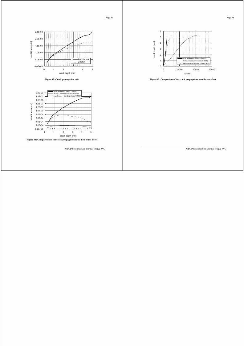
7/31/2019 Nea Study of Thermal Fatigue
http://slidepdf.com/reader/full/nea-study-of-thermal-fatigue 105/147
0.0E+00
5.0E-04
1.0E-03
1.5E-03
0 1 2 3 4 5
crack depth [mm]
d a
/ d N
[ m m
/ c y
BenchmarkCRIEPI
Figure 43: Crack propagation rate
0.0E+00
2.0E-04
4.0E-04
6.0E-04
8.0E-04
1.0E-03
1.2E-03
1.4E-03
1.6E-03
1.8E-03
2.0E-03
0 1 2 3 4 5
crack depth [mm]
d a
/ d N
[ m m
/ c y c
l e ]
With membrane stress-CRIEPIWithout membrane stress-CRIEPImembrane bending stress-CRIEPI
Figure 44: Comparison of the crack propagation rate: membrane effect
OECD benchmark on thermal fatigue-JNC
0
1
2
3
0 20000 40000 60000
cycles
c r a c
k d e p
t h [ m
With membrane stress-CRIEPIWithout membrane stress-CRIEPImembrane bending stress-CRIEPI
Figure 45: Comparison of the crack propagation: membrane effect
OECD benchmark on thermal fatigue-JNC
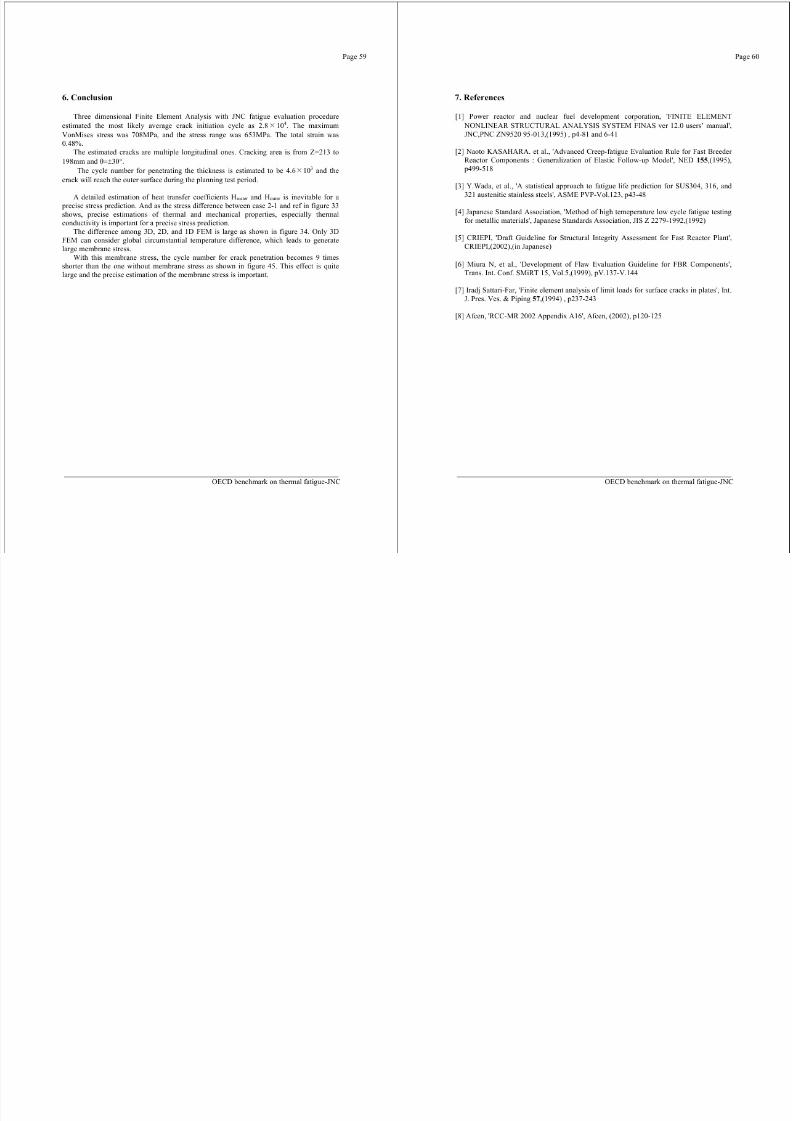
7/31/2019 Nea Study of Thermal Fatigue
http://slidepdf.com/reader/full/nea-study-of-thermal-fatigue 106/147
7/31/2019 Nea Study of Thermal Fatigue
http://slidepdf.com/reader/full/nea-study-of-thermal-fatigue 107/147
DET NORSKEVERITAS
R ESEARCH R EPORT
DET NORSKEVERITAS ABDNV Technology Sweden
Report title:Thermal Fatigue Benchmark Final
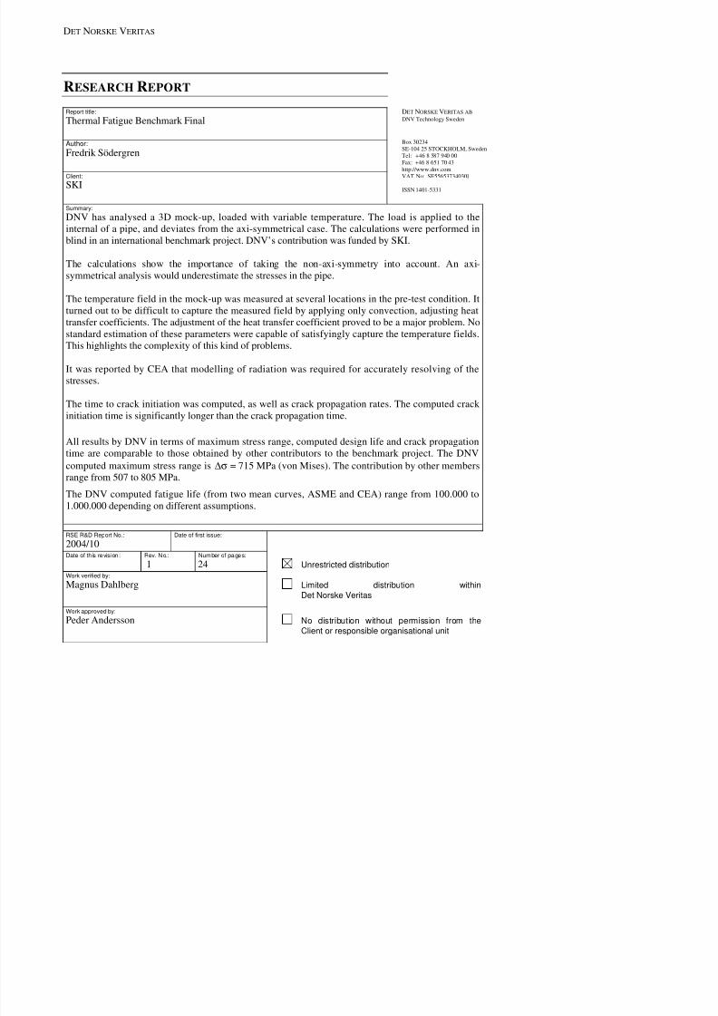
7/31/2019 Nea Study of Thermal Fatigue
http://slidepdf.com/reader/full/nea-study-of-thermal-fatigue 108/147
Box 30234SE-104 25 STOCKHOLM, SwedenTel: +46 8 587 940 00Fax: +46 8 651 70 43http://www.dnv.comVAT No: SE556537340301
ISSN 1401-5331
Author:Fredrik Södergren
Client:
SKI
Summary:
DNV has analysed a 3D mock-up, loaded with variable temperature. The load is applied to theinternal of a pipe, and deviates from the axi-symmetrical case. The calculations were performed inblind in an international benchmark project. DNV’s contribution was funded by SKI.
The calculations show the importance of taking the non-axi-symmetry into account. An axi-symmetrical analysis would underestimate the stresses in the pipe.
The temperature field in the mock-up was measured at several locations in the pre-test condition. Itturned out to be difficult to capture the measured field by applying only convection, adjusting heattransfer coefficients. The adjustment of the heat transfer coefficient proved to be a major problem. Nostandard estimation of these parameters were capable of satisfyingly capture the temperature fields.This highlights the complexity of this kind of problems.
It was reported by CEA that modelling of radiation was required for accurately resolving of thestresses.
The time to crack initiation was computed, as well as crack propagation rates. The computed crackinitiation time is significantly longer than the crack propagation time.
All results by DNV in terms of maximum stress range, computed design life and crack propagationtime are comparable to those obtained by other contributors to the benchmark project. The DNV
computed maximum stress range isΔσ = 715 MPa (von Mises). The contribution by other membersrange from 507 to 805 MPa.The DNV computed fatigue life (from two mean curves, ASME and CEA) range from 100.000 to1 000 000 d di diff t ti
DET NORSKEVERITAS
Report No: 2004/10, rev. 1
RESEARCHREPORT
Table of Content Page
7/31/2019 Nea Study of Thermal Fatigue
http://slidepdf.com/reader/full/nea-study-of-thermal-fatigue 109/147
1. INTRODUCTION........................................................................................................1
2. GENERAL INPUT DATA ..........................................................................................1
3. THERMAL ANALYSIS..............................................................................................34. STRESS RESULTS ..................................................................................................... 8
5. FATIGUE.....................................................................................................................9
6. CRACK PROPAGATION ANALYSIS ....................................................................11
7. CONCLUSIONS........................................................................................................15REFERENCES......................................................................................................................... 15
TABLE OF REVISIONS ......................................................................................................... 16
APPENDIX A........................................................................................................................... 17
DET NORSKEVERITAS
Report No: 2004/10, rev. 1
RESEARCHREPORT
1. INTRODUCTION
Thi k i f d f h l l i f h CEA j h l f i
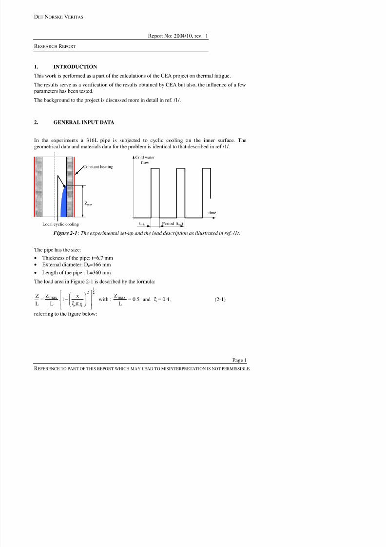
7/31/2019 Nea Study of Thermal Fatigue
http://slidepdf.com/reader/full/nea-study-of-thermal-fatigue 110/147
This work is performed as a part of the calculations of the CEA project on thermal fatigue.The results serve as a verification of the results obtained by CEA but also, the influence of a fewparameters has been tested.The background to the project is discussed more in detail in ref. /1/.
2. GENERAL INPUT DATA
In the experiments a 316L pipe is subjected to cyclic cooling on the inner surface. Thegeometrical data and materials data for the problem is identical to that described in ref /1/.
Zmax
Local cyclic cooling
Constant heating
time
Cold waterflow
tcold Period (ttot)
Figure 2-1 : The experimental set-up and the load description as illustrated in ref. /1/.
The pipe has the size:• Thickness of the pipe: t=6.7 mm• External diameter: De=166 mm
L h f h i L 360
DET NORSKE VERITAS
Report No: 2004/10, rev. 1
RESEARCHREPORT
Z
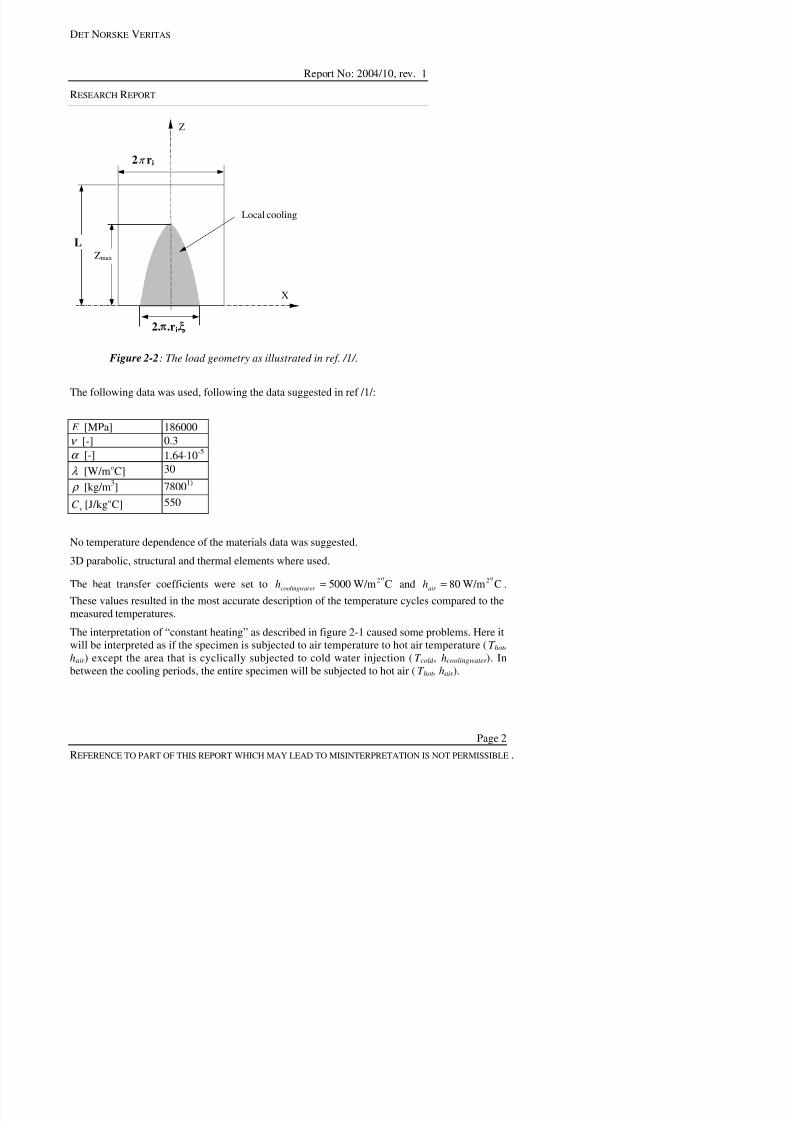
7/31/2019 Nea Study of Thermal Fatigue
http://slidepdf.com/reader/full/nea-study-of-thermal-fatigue 111/147
X
Local cooling
2π r i
Zmax
L
2. .r i.
Figure 2-2 : The load geometry as illustrated in ref. /1/.
The following data was used, following the data suggested in ref /1/:
E [MPa] 186000ν [-] 0.3α [-] 1.64 10-5
λ C][W/mo 30 ρ [kg/m3] 78001)
vC C][J/kgo 550
No temperature dependence of the materials data was suggested.
DET NORSKE VERITAS
Report No: 2004/10, rev. 1
RESEARCHREPORT
3. THERMALANALYSISThe model was run with a period time of t tot = 190 s, and the cooling time ist cold = 15 s. The
di t t T 650oC dT 17 oC
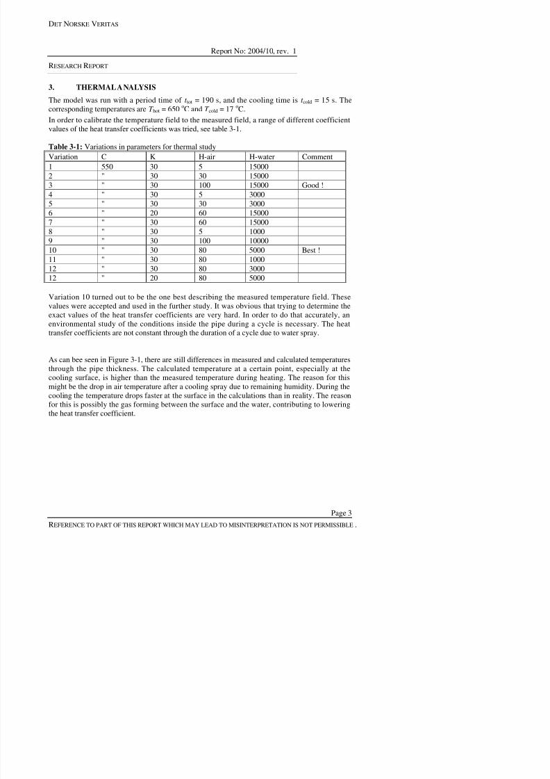
7/31/2019 Nea Study of Thermal Fatigue
http://slidepdf.com/reader/full/nea-study-of-thermal-fatigue 112/147
corresponding temperatures areT hot = 650oC andT cold = 17 oC.In order to calibrate the temperature field to the measured field, a range of different coefficientvalues of the heat transfer coefficients was tried, see table 3-1.
Table 3-1: Variations in parameters for thermal studyVariation C K H-air H-water Comment1 550 30 5 150002 " 30 30 150003 " 30 100 15000 Good !4 " 30 5 30005 " 30 30 30006 " 20 60 150007 " 30 60 150008 " 30 5 10009 " 30 100 1000010 " 30 80 5000 Best !11 " 30 80 100012 " 30 80 300012 " 20 80 5000
Variation 10 turned out to be the one best describing the measured temperature field. Thesevalues were accepted and used in the further study. It was obvious that trying to determine theexact values of the heat transfer coefficients are very hard. In order to do that accurately, anenvironmental study of the conditions inside the pipe during a cycle is necessary. The heattransfer coefficients are not constant through the duration of a cycle due to water spray.
As can bee seen in Figure 3-1, there are still differences in measured and calculated temperaturesthrough the pipe thickness. The calculated temperature at a certain point, especially at thecooling surface, is higher than the measured temperature during heating. The reason for thismight be the drop in air temperature after a cooling spray due to remaining humidity During the
DET NORSKE VERITAS
Report No: 2004/10, rev. 1
RESEARCHREPORT
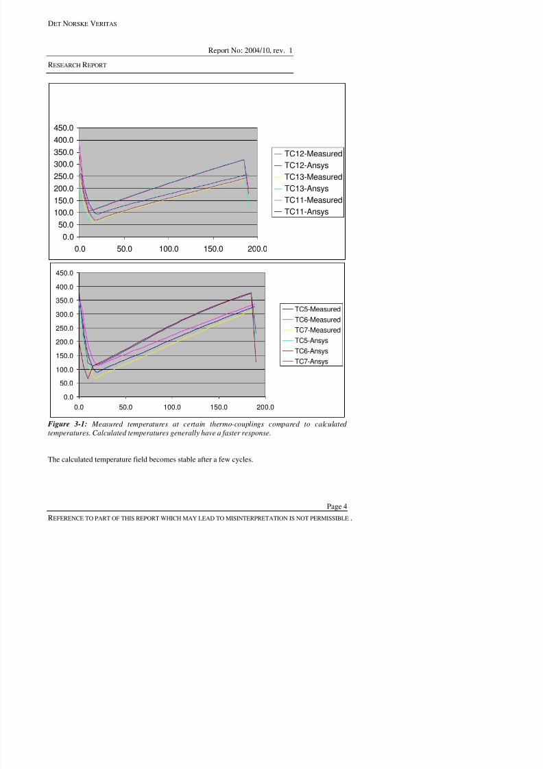
7/31/2019 Nea Study of Thermal Fatigue
http://slidepdf.com/reader/full/nea-study-of-thermal-fatigue 113/147
0.050.0
100.0150.0200.0250.0300.0350.0
400.0450.0
0.0 50.0 100.0 150.0 200.0
TC12-MeasuredTC12-AnsysTC13-MeasuredTC13-AnsysTC11-MeasuredTC11-Ansys
100.0
150.0
200.0
250.0
300.0
350.0
400.0
450.0
TC5-MeasuredTC6-MeasuredTC7-MeasuredTC5-Ansys
TC6-AnsysTC7-Ansys
DET NORSKE VERITAS
Report No: 2004/10, rev. 1
RESEARCHREPORT
1
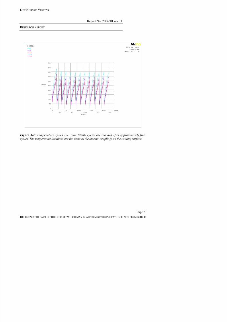
7/31/2019 Nea Study of Thermal Fatigue
http://slidepdf.com/reader/full/nea-study-of-thermal-fatigue 114/147
Figure 3-2: Temperature cycles over time. Stable cycles are reached after approximately fivecycles. The temperature locations are the same as the thermo-couplings on the cooling surface.
0
50
100
150
200
250
300
350
400
450
500
VALU
0
250
500
750
1000
1250
1500
1750
2000
2250
2500
TIME
SEP 15 200415:59:34
PLOT NO. 1
POST26
TC4TC7TC10TC13TC16
DET NORSKE VERITAS
Report No: 2004/10, rev. 1
RESEARCHREPORT
1
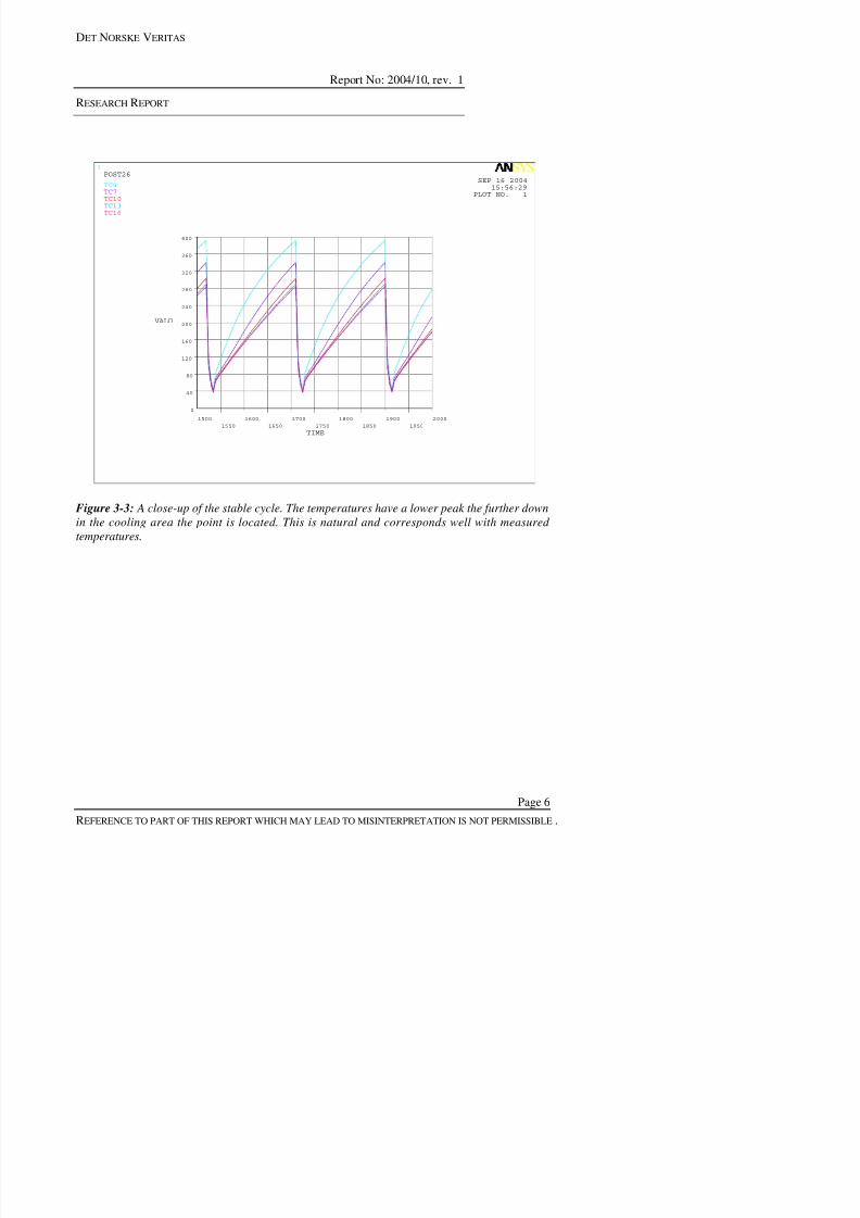
7/31/2019 Nea Study of Thermal Fatigue
http://slidepdf.com/reader/full/nea-study-of-thermal-fatigue 115/147
Figure 3-3: A close-up of the stable cycle. The temperatures have a lower peak the further downin the cooling area the point is located. This is natural and corresponds well with measured temperatures.
0
40
80
120
160
200
240
280
320
360
400
VALU
1500
1550
1600
1650
1700
1750
1800
1850
1900
1950
2000
TIME
SEP 16 200415:56:29
PLOT NO. 1
POST26
TC4TC7TC10TC13TC16
DET NORSKE VERITAS
Report No: 2004/10, rev. 1
RESEARCHREPORT
1
NODAL SOLUTION
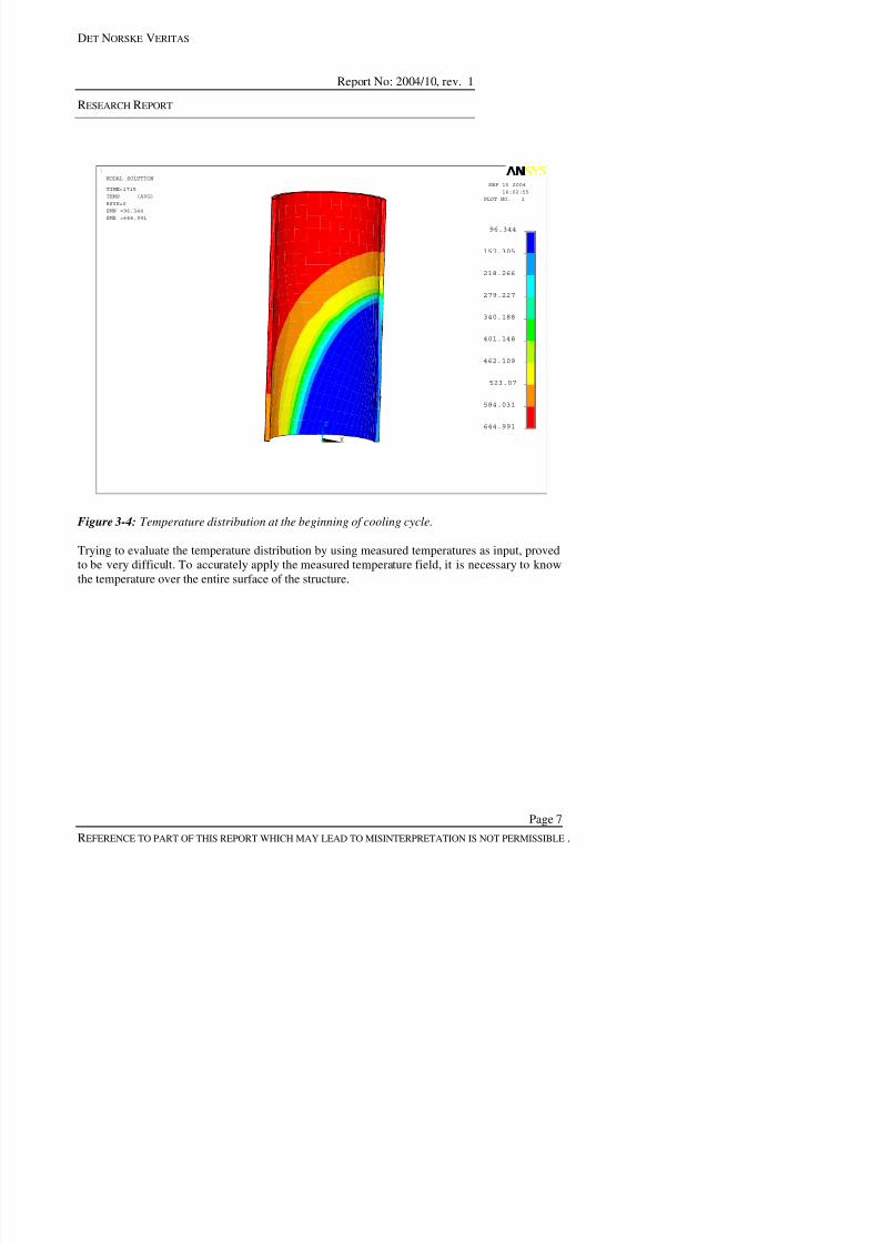
7/31/2019 Nea Study of Thermal Fatigue
http://slidepdf.com/reader/full/nea-study-of-thermal-fatigue 116/147
Figure 3-4: Temperature distribution at the beginning of cooling cycle.
Trying to evaluate the temperature distribution by using measured temperatures as input, provedto be very difficult. To accurately apply the measured temperature field, it is necessary to knowthe temperature over the entire surface of the structure.
MN
MX
XY
Z
96.344
157.305
218.266
279.227
340.188
401.148
462.109
523.07
584.031
644.991
SEP 15 2004
16:02:55
PLOT NO. 1
NODAL SOLUTION
TIME=1715
TEMP (AVG)
RSYS=0
SMN =96.344
SMX =644.991
DET NORSKE VERITAS
Report No: 2004/10, rev. 1
RESEARCHREPORT
4. STRESS RESULTS
Th l d i d f f ll l i FE l i W h i i i h f h
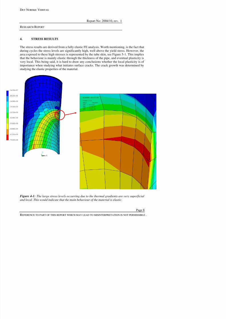
7/31/2019 Nea Study of Thermal Fatigue
http://slidepdf.com/reader/full/nea-study-of-thermal-fatigue 117/147
The stress results are derived from a fully elastic FE analysis. Worth mentioning, is the fact thatduring cycles the stress levels are significantly high, well above the yield stress. However, thearea exposed to these high stresses is represented by the tube skin, see Figure 5-1. This impliesthat the behaviour is mainly elastic through the thickness of the pipe, and eventual plasticity isvery local. This being said, it is hard to draw any conclusions whether the local plasticity is of importance when studying what initiates surface cracks. The crack growth was determined bystudying the elastic properties of the material.
1ELEMENT SOLUTION
TIME=1715
SEQV (NOAVG)
DMX =.003994
SMN =.147E+07
SMX =.755E+09
XY
Z
.147E+07
.852E+08
.169E+09
.253E+09
.337E+09
.420E+09
.504E+09
.588E+09
.672E+09
.755E+09
DET NORSKE VERITAS
Report No: 2004/10, rev. 1
RESEARCHREPORT
SEP 23 200411:22:19
PLOT NO. 1
MEMBRANEMEM+BENDTOTAL
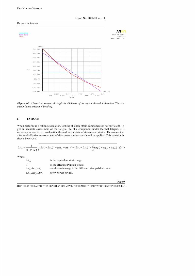
7/31/2019 Nea Study of Thermal Fatigue
http://slidepdf.com/reader/full/nea-study-of-thermal-fatigue 118/147
Figure 4-2: Linearised stresses through the thickness of the pipe in the axial direction. There isa significant amount of bending.
5. FATIGUE
When performing a fatigue evaluation, looking at single strain components is not sufficient. Toget an accurate assessment of the fatigue life of a component under thermal fatigue, it isnecessary to take in to consideration the multi-axial state of stresses and strains. This means thata form of effective measurement of the current strain state should be applied. This equation is
-2638.979
-1592.027
-545.075
501.876
1548.828
2595.780
3642.732
4689.684
5736.636
6783.588
7830.536
(x10**5)
SY
0
.834
1.668
2.502
3.336
4.17
5.004
5.838
6.672
7.506
8.343
DIST
(x10**-3)
DET NORSKE VERITAS
Report No: 2004/10, rev. 1
RESEARCHREPORT
Since the high strain levels in the radial direction will contribute to plasticity, but the amount of plasticity is hard to determine without the use of very sophisticated material models, anassumption of total incompressibility is made. This is generally a conservative assumption.From the equation below the corrected radial strain can then be calculated /4/
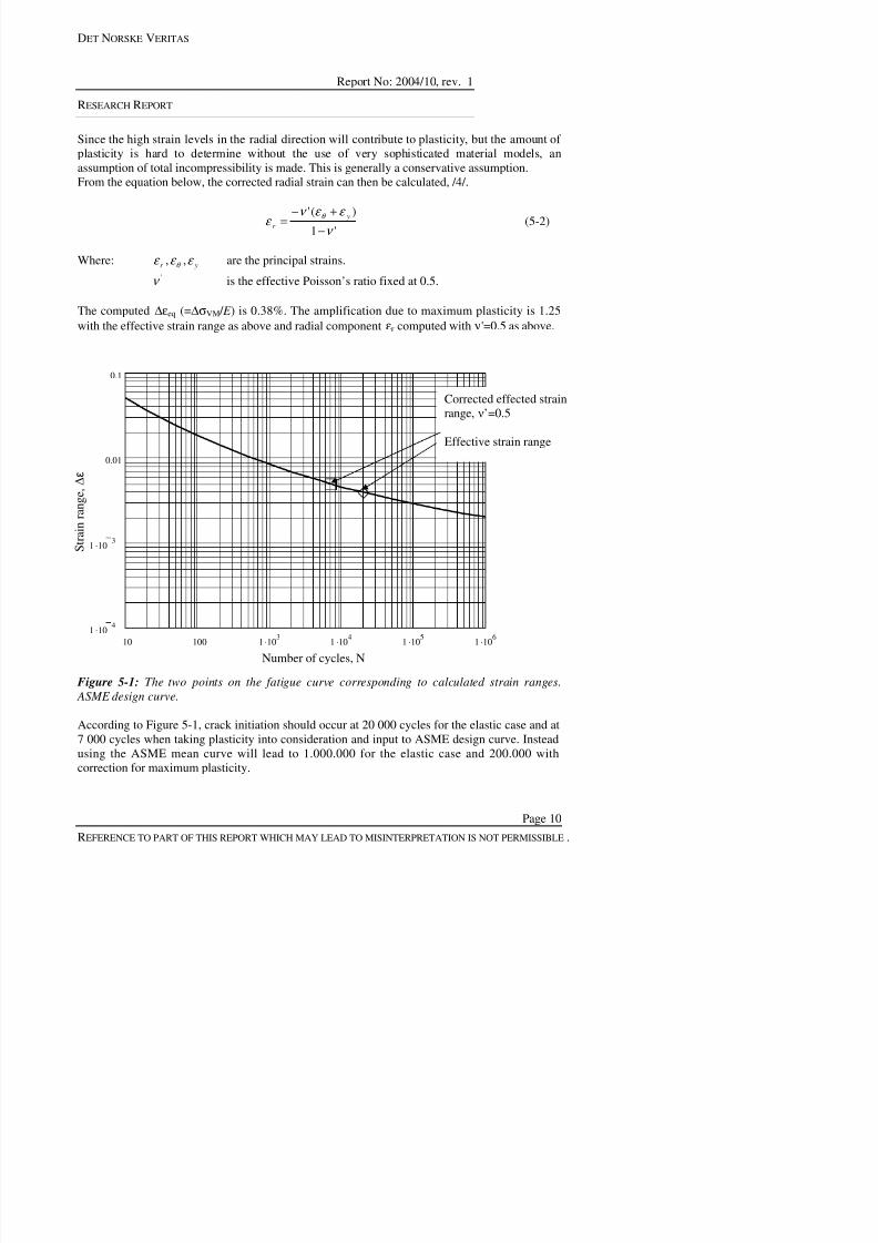
7/31/2019 Nea Study of Thermal Fatigue
http://slidepdf.com/reader/full/nea-study-of-thermal-fatigue 119/147
From the equation below, the corrected radial strain can then be calculated, /4/.
'1)('
ν ε ε ν
ε θ
−+−
= yr (5-2)
Where: r ε , θ ε , yε are the principal strains.'ν is the effective Poisson’s ratio fixed at 0.5.
The computedΔεeq (=ΔσVM / E ) is 0.38%. The amplification due to maximum plasticity is 1.25with the effective strain range as above and radial componentεr computed withν'=0.5 as above.
1 .10 3
0.01
0.1
S t r a
i n r a n g e
, Δ ε
Corrected effected strainrange, ν ’=0.5
Effective strain range
DET NORSKE VERITAS
Report No: 2004/10, rev. 1
RESEARCHREPORT
Instead using the CEA proposed fatigue curve leads to other results. Another measure of theeffective strain should probably be used, with ( )
eqeq ε ν ε Δ+=Δ3
'12' as input to the CEA fatigue
Th l i ll d i ill b 'Δ 0 33% Th lifi i d i
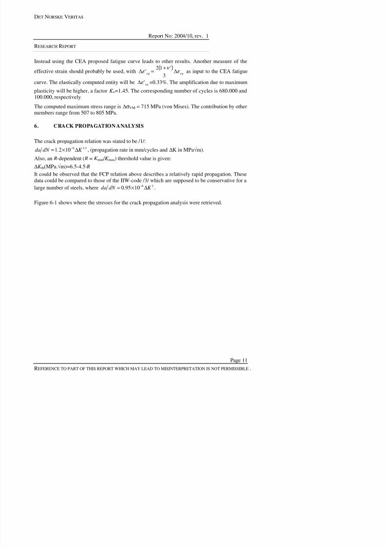
7/31/2019 Nea Study of Thermal Fatigue
http://slidepdf.com/reader/full/nea-study-of-thermal-fatigue 120/147
curve. The elastically computed entity will be eq'ε Δ =0.33%. The amplification due to maximumplasticity will be higher, a factorK ν=1.45. The corresponding number of cycles is 680.000 and100.000, respectively.
The computed maximum stress range isΔσVM = 715 MPa (von Mises). The contribution by othermembers range from 507 to 805 MPa.
6. CRACK PROPAGATION ANALYSIS
The crack propagation relation was stated to be /1/:3.38102.1 K dN da Δ×= − , (propagation rate in mm/cycles andΔK in MPa√m).
Also, anR-dependent ( R = K min / K max) threshold value is given:ΔK th(MPa.√m)=6.5-4.5· RIt could be observed that the FCP relation above describes a relatively rapid propagation. Thesedata could be compared to those of the IIW-code /3/ which are supposed to be conservative for alarge number of steels, where 381095.0 K dN da Δ×= − .
Figure 6-1 shows where the stresses for the crack propagation analysis were retrieved.
DET NORSKE VERITAS
Report No: 2004/10, rev. 1
RESEARCHREPORT
ELEMENT SOLUTION
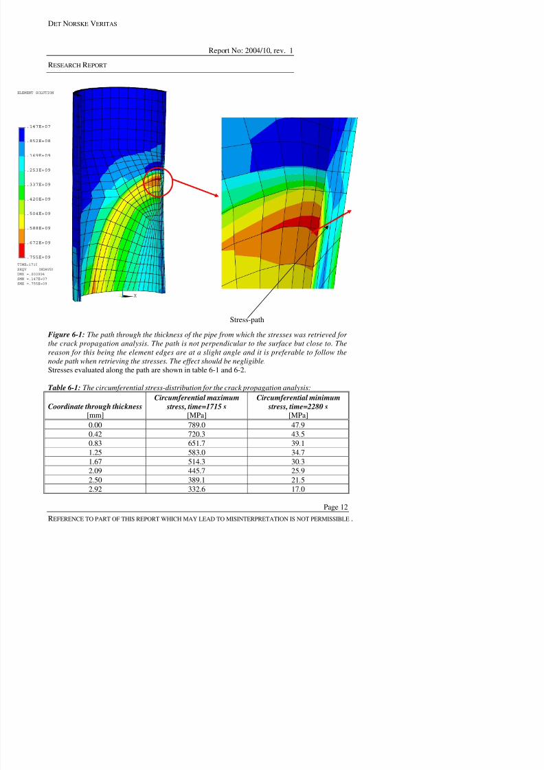
7/31/2019 Nea Study of Thermal Fatigue
http://slidepdf.com/reader/full/nea-study-of-thermal-fatigue 121/147
Figure 6-1: The path through the thickness of the pipe from which the stresses was retrieved for the crack propagation analysis. The path is not perpendicular to the surface but close to. The
reason for this being the element edges are at a slight angle and it is preferable to follow thenode path when retrieving the stresses. The effect should be negligible.Stresses evaluated along the path are shown in table 6-1 and 6-2.
XY
Z
.147E+07
.852E+08
.169E+09
.253E+09
.337E+09
.420E+09
.504E+09
.588E+09
.672E+09
.755E+09
TIME=1715SEQV (NOAVG)DMX =.003994SMN =.147E+07SMX =.755E+09
Stress-path
DET NORSKE VERITAS
Report No: 2004/10, rev. 1
RESEARCHREPORT
3.34 276.0 12.53.75 219.4 8.034.17 162.9 3.564 59 122 4 -0 95
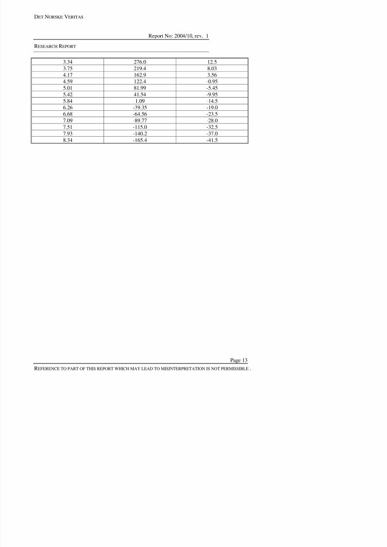
7/31/2019 Nea Study of Thermal Fatigue
http://slidepdf.com/reader/full/nea-study-of-thermal-fatigue 122/147
4.59 122.4 0.955.01 81.99 -5.455.42 41.54 -9.955.84 1.09 -14.5
6.26 -39.35 -19.06.68 -64.56 -23.57.09 -89.77 -28.07.51 -115.0 -32.57.93 -140.2 -37.08.34 -165.4 -41.5
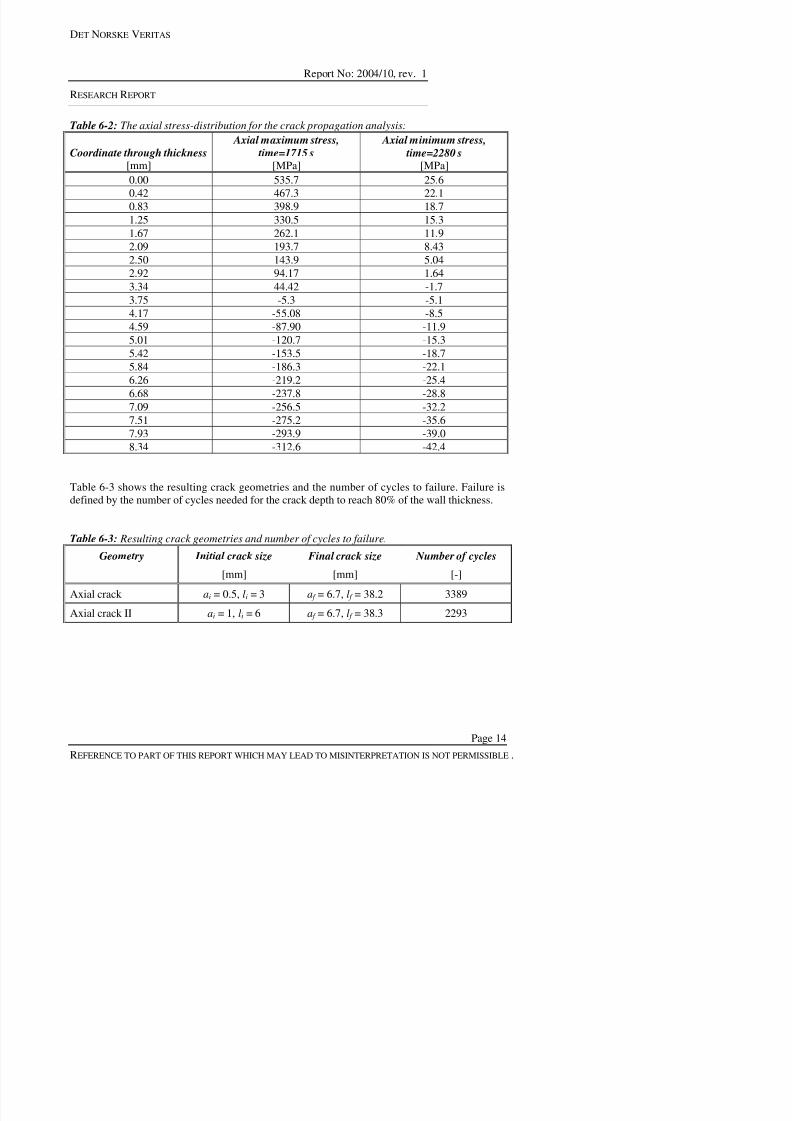
7/31/2019 Nea Study of Thermal Fatigue
http://slidepdf.com/reader/full/nea-study-of-thermal-fatigue 123/147
DET NORSKE VERITAS
Report No: 2004/10, rev. 1
RESEARCHREPORT
7. CONCLUSIONS
The calculations show the importance of taking the non-axi-symmetry into account. An axi-
7/31/2019 Nea Study of Thermal Fatigue
http://slidepdf.com/reader/full/nea-study-of-thermal-fatigue 124/147
p g y ysymmetrical analysis would underestimate the stresses in the pipe.
The temperature field in the mock-up was measured at several locations. It turned out to bedifficult to capture the measured field by applying only convection, adjusting heat transfercoefficients.All results by DNV in terms of maximum stress range, computed design life and crackpropagation time are comparable to those obtained other contributors to the benchmark project,ref /6/.The experiments turned out to different from the pre-test conditions. However, it was observedthat the mock-up load was larger than intended, ref /6/. An increase of the stresses to the order of 50% of the stresses was estimated. This severely hampers the comparison between the computedfatigue results and the results from the fatigue testing.However, the location and orientation of the dominant crack is well in agreement with ourresults.All results by DNV in terms of maximum stress range, computed design life and crackpropagation time are comparable to those obtained by other contributors to the benchmarkproject. The DNV computed maximum stress range isΔσ = 715 MPa (von Mises). The
contribution by other members range from 507 to 805 MPa.The DNV computed fatigue life (from two mean curves) range from 100.000 to 1.000.000depending on different assumptions.
REFERENCES
/1/ Chapuliot S., Payen T., Benchmark proposal on thermal fatigue problem,OECD/NEA/CSNI Integrity and Ageing Working Group, September 2001 /2/ Chapuliot S., Payen T., Mathet M.,OECD Benchmark proposal on thermal fatigue
bl P iti d d th i f th OECD/NEA/CSNI A g t 2002
DET NORSKE VERITAS
Report No: 2004/10, rev. 1
RESEARCHREPORT
TABLE OF REVISIONS

7/31/2019 Nea Study of Thermal Fatigue
http://slidepdf.com/reader/full/nea-study-of-thermal-fatigue 125/147
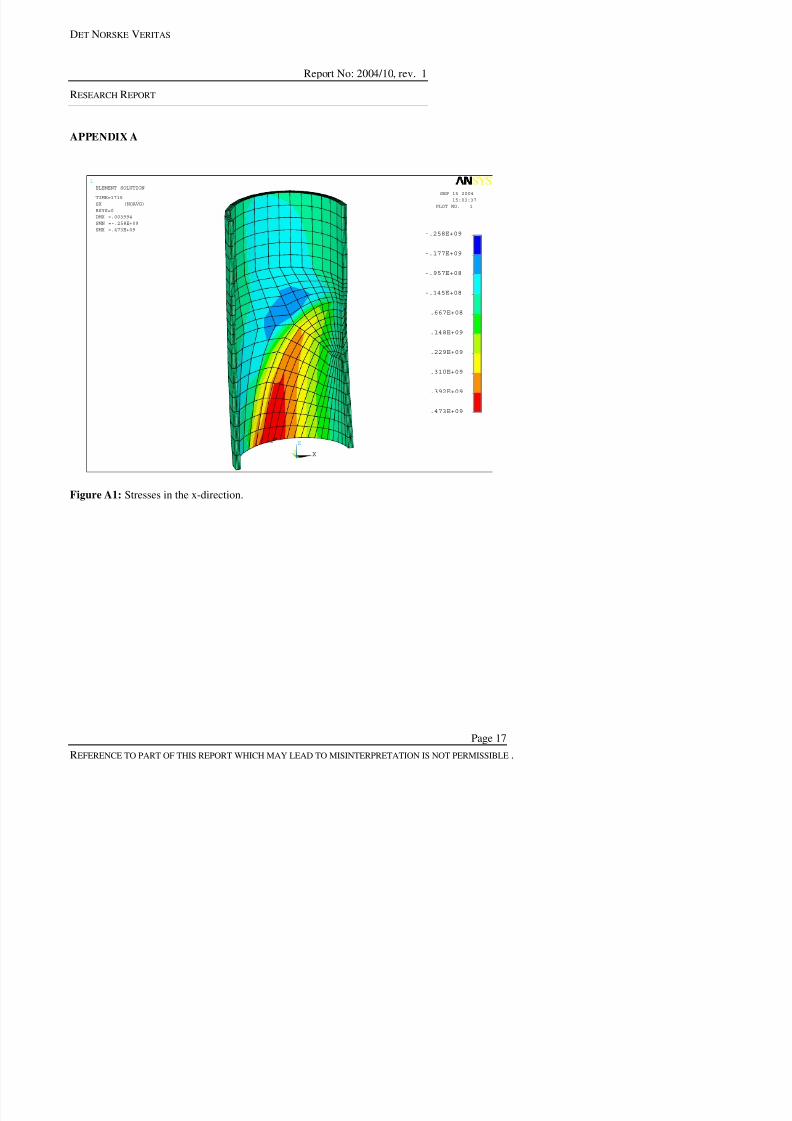
7/31/2019 Nea Study of Thermal Fatigue
http://slidepdf.com/reader/full/nea-study-of-thermal-fatigue 126/147
DET NORSKE VERITAS
Report No: 2004/10, rev. 1
RESEARCHREPORT
1
SEP 15 2004
15:03:48
ELEMENT SOLUTION
TIME=1715
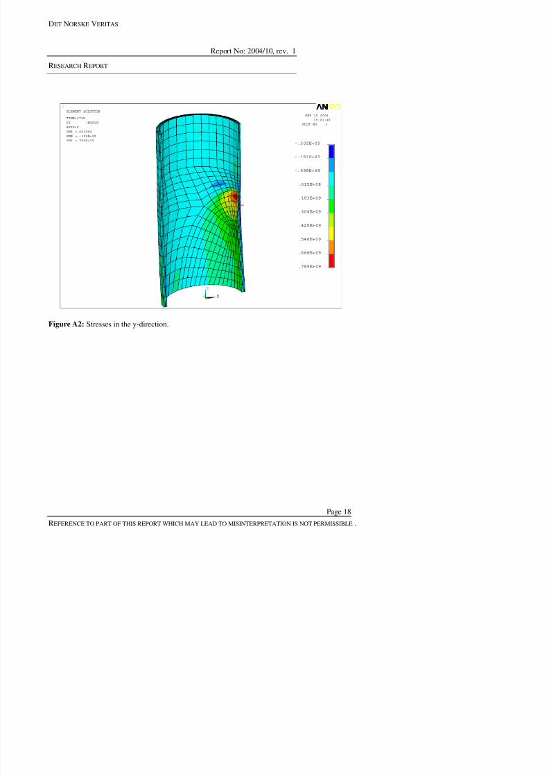
7/31/2019 Nea Study of Thermal Fatigue
http://slidepdf.com/reader/full/nea-study-of-thermal-fatigue 127/147
Figure A2: Stresses in the y-direction.
MN
MX
XY
Z
-.302E+09
-.181E+09
-.598E+08
.615E+08
.183E+09
.304E+09
.425E+09
.546E+09
.668E+09
.789E+09
PLOT NO. 1SY (NOAVG)
RSYS=0
DMX =.003994
SMN =-.302E+09
SMX =.789E+09
DET NORSKE VERITAS
Report No: 2004/10, rev. 1
RESEARCHREPORT
1
SEP 15 2004
15:04:04
ELEMENT SOLUTION
TIME=1715
SZ (NOAVG)
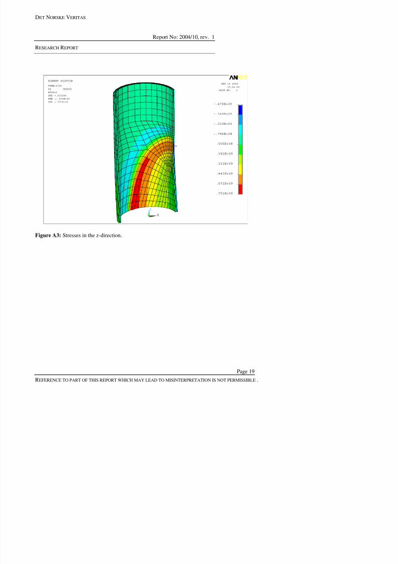
7/31/2019 Nea Study of Thermal Fatigue
http://slidepdf.com/reader/full/nea-study-of-thermal-fatigue 128/147
Figure A3: Stresses in the z-direction.
MN
MX
XY
Z
-.470E+09
-.340E+09
-.210E+09
-.796E+08
.505E+08
.181E+09
.311E+09
.441E+09
.571E+09
.701E+09
PLOT NO. 1SZ (NOAVG)
RSYS=0
DMX =.003994
SMN =-.470E+09
SMX =.701E+09
DET NORSKE VERITAS
Report No: 2004/10, rev. 1
RESEARCHREPORT
1
MN SEP 15 2004
15:04:19
PLOT NO 1
ELEMENT SOLUTION
TIME=1715
SEQV (NOAVG)
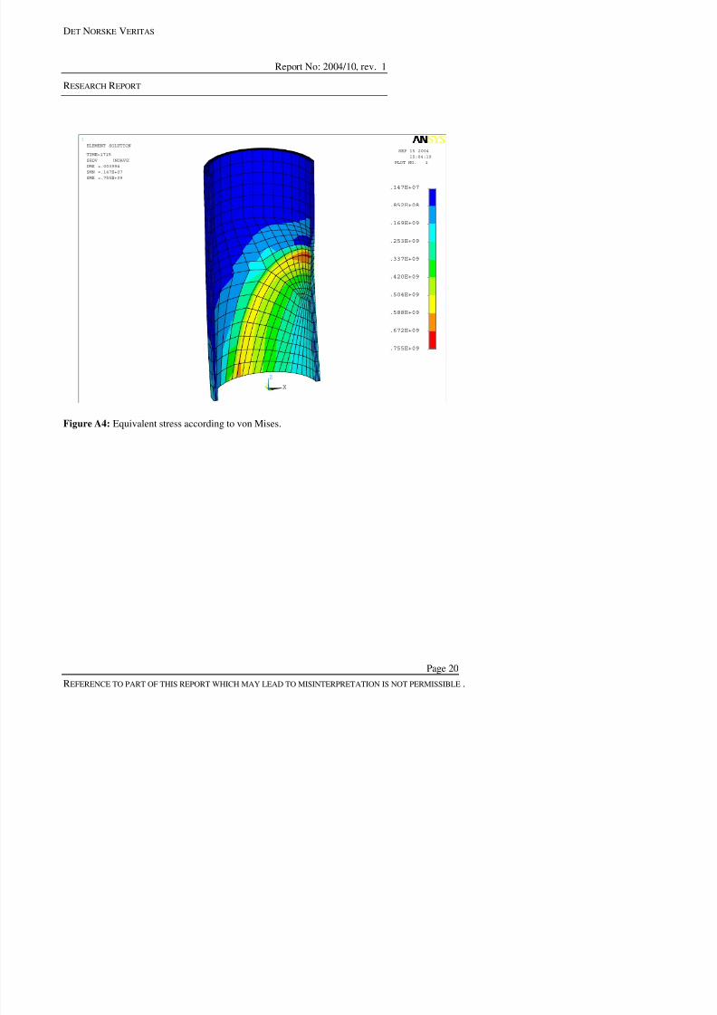
7/31/2019 Nea Study of Thermal Fatigue
http://slidepdf.com/reader/full/nea-study-of-thermal-fatigue 129/147
Figure A4: Equivalent stress according to von Mises.
MX
XY
Z
.147E+07
.852E+08
.169E+09
.253E+09
.337E+09
.420E+09
.504E+09
.588E+09
.672E+09
.755E+09
PLOT NO. 1SEQV (NOAVG)
DMX =.003994
SMN =.147E+07
SMX =.755E+09
DET NORSKE VERITAS
Report No: 2004/10, rev. 1
RESEARCHREPORT
1
SEP 15 2004
15:06:14
PLOT NO 1
ELEMENT SOLUTION
TIME=1715
SX (NOAVG)
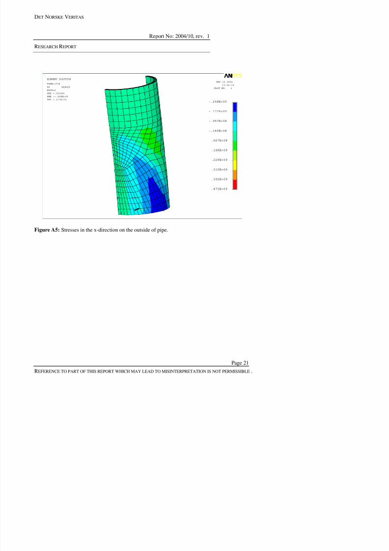
7/31/2019 Nea Study of Thermal Fatigue
http://slidepdf.com/reader/full/nea-study-of-thermal-fatigue 130/147
Figure A5: Stresses in the x-direction on the outside of pipe.
MNMXX Y
Z
-.258E+09
-.177E+09
-.957E+08
-.145E+08
.667E+08
.148E+09
.229E+09
.310E+09
.392E+09
.473E+09
PLOT NO. 1RSYS=0
DMX =.003994
SMN =-.258E+09
SMX =.473E+09
DET NORSKE VERITAS
Report No: 2004/10, rev. 1
RESEARCHREPORT
1
SEP 15 2004
15:06:27
PLOT NO. 1
ELEMENT SOLUTION
TIME=1715
SY (NOAVG)
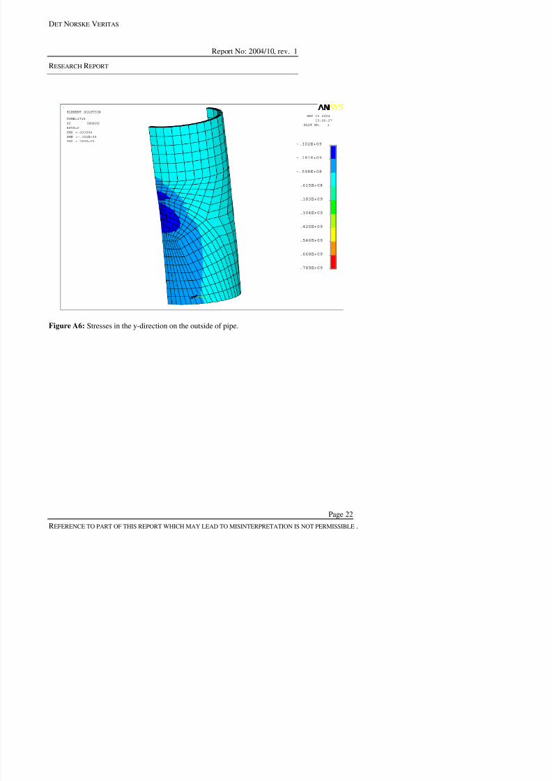
7/31/2019 Nea Study of Thermal Fatigue
http://slidepdf.com/reader/full/nea-study-of-thermal-fatigue 131/147
Figure A6: Stresses in the y-direction on the outside of pipe.
MN
MX
X Y
Z
-.302E+09
-.181E+09
-.598E+08
.615E+08
.183E+09
.304E+09
.425E+09
.546E+09
.668E+09
.789E+09
RSYS=0
DMX =.003994
SMN =-.302E+09
SMX =.789E+09
DET NORSKE VERITAS
Report No: 2004/10, rev. 1
RESEARCHREPORT
1
SEP 15 2004
15:06:39
PLOT NO. 1
ELEMENT SOLUTION
TIME=1715
SZ (NOAVG)
RSYS 0
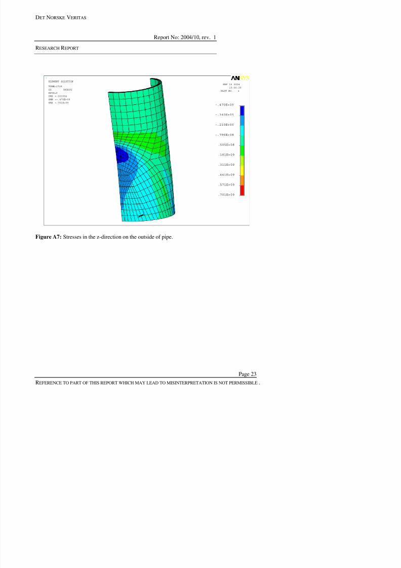
7/31/2019 Nea Study of Thermal Fatigue
http://slidepdf.com/reader/full/nea-study-of-thermal-fatigue 132/147
Figure A7: Stresses in the z-direction on the outside of pipe.
MN
MXX Y
Z
-.470E+09
-.340E+09
-.210E+09
-.796E+08
.505E+08
.181E+09
.311E+09
.441E+09
.571E+09
.701E+09
RSYS=0
DMX =.003994
SMN =-.470E+09
SMX =.701E+09
DET NORSKE VERITAS
Report No: 2004/10, rev. 1
RESEARCHREPORT
1
MN
SEP 15 2004
15:31:11
PLOT NO. 1
ELEMENT SOLUTION
TIME=1715
SEQV (NOAVG)
DMX = 003994
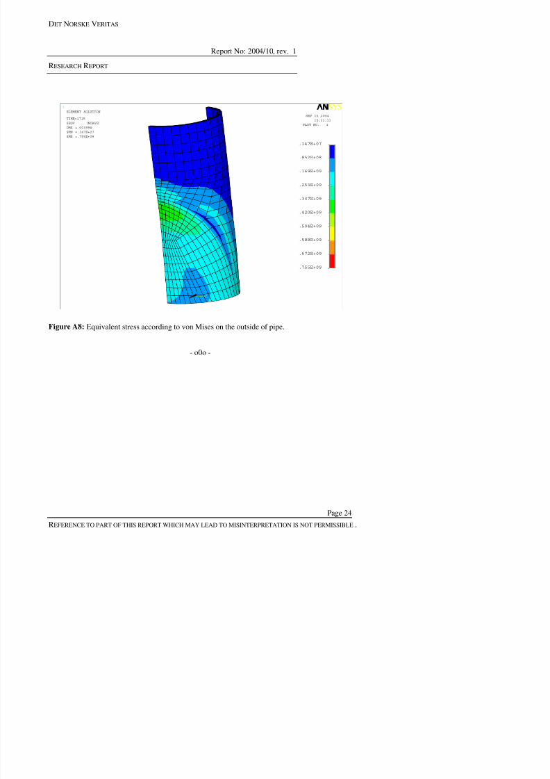
7/31/2019 Nea Study of Thermal Fatigue
http://slidepdf.com/reader/full/nea-study-of-thermal-fatigue 133/147
Figure A8: Equivalent stress according to von Mises on the outside of pipe.
- o0o -
MX
X Y
Z
.147E+07
.852E+08
.169E+09
.253E+09
.337E+09
.420E+09
.504E+09
.588E+09
.672E+09
.755E+09
DMX =.003994
SMN =.147E+07
SMX =.755E+09
7/31/2019 Nea Study of Thermal Fatigue
http://slidepdf.com/reader/full/nea-study-of-thermal-fatigue 134/147
7/31/2019 Nea Study of Thermal Fatigue
http://slidepdf.com/reader/full/nea-study-of-thermal-fatigue 135/147
7/31/2019 Nea Study of Thermal Fatigue
http://slidepdf.com/reader/full/nea-study-of-thermal-fatigue 136/147
7/31/2019 Nea Study of Thermal Fatigue
http://slidepdf.com/reader/full/nea-study-of-thermal-fatigue 137/147
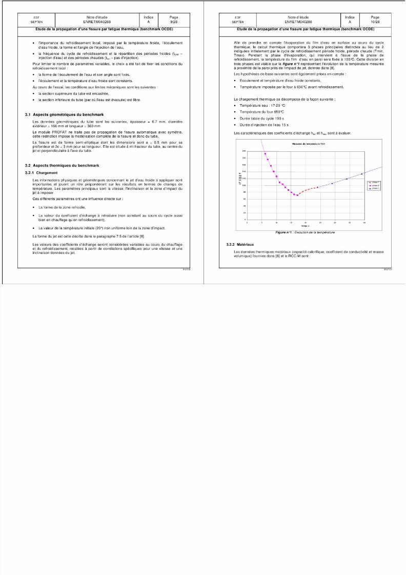
7/31/2019 Nea Study of Thermal Fatigue
http://slidepdf.com/reader/full/nea-study-of-thermal-fatigue 138/147
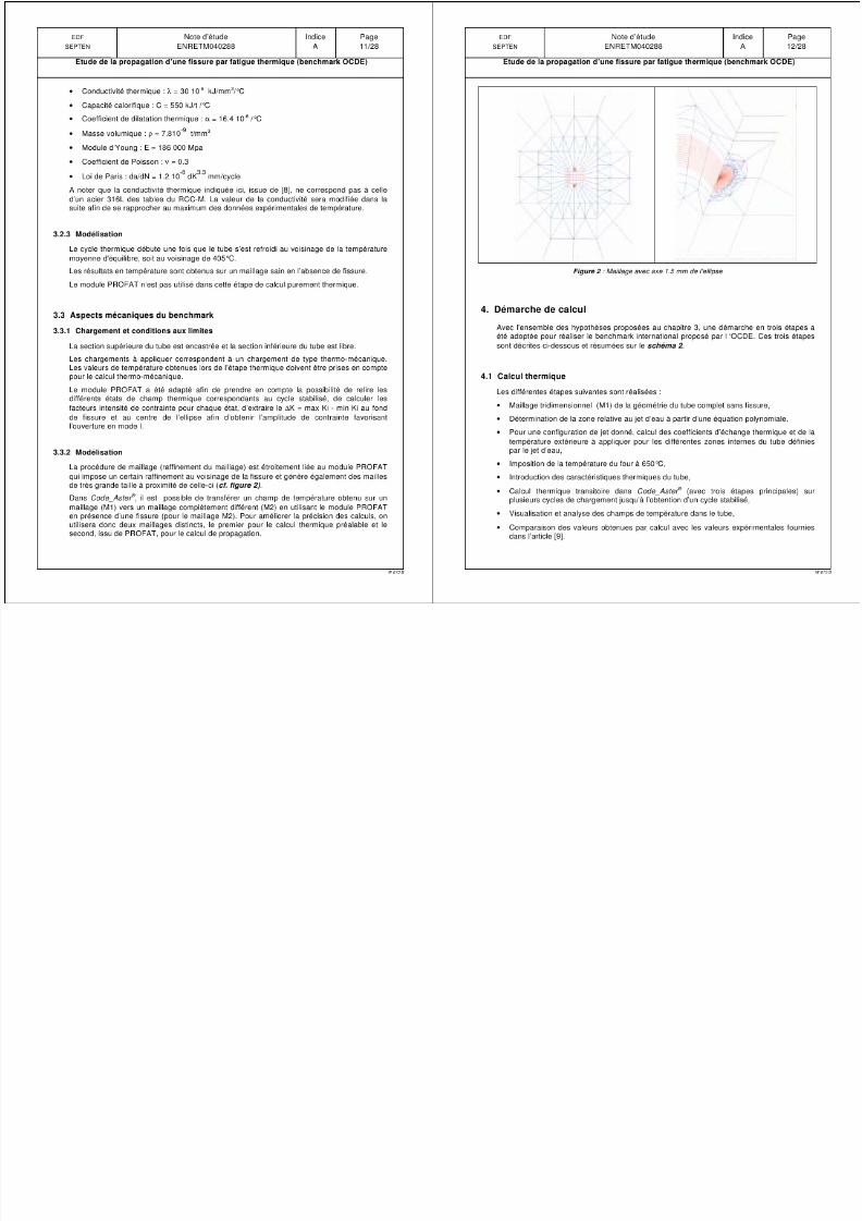
7/31/2019 Nea Study of Thermal Fatigue
http://slidepdf.com/reader/full/nea-study-of-thermal-fatigue 139/147
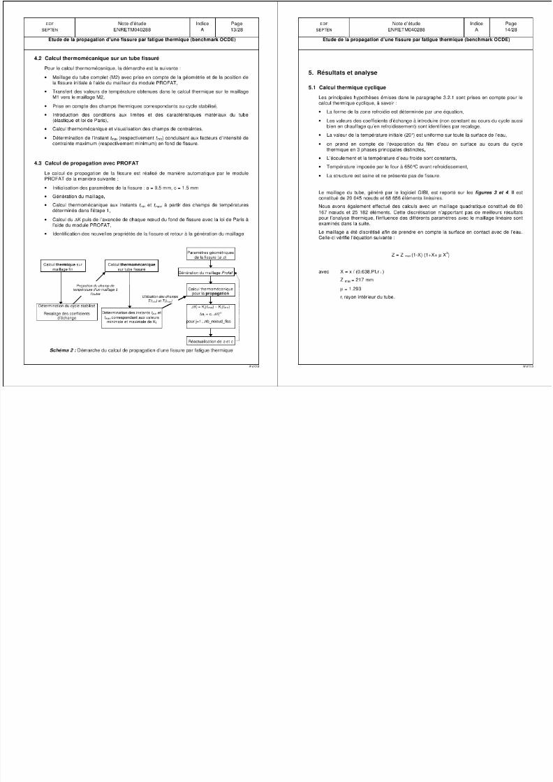
7/31/2019 Nea Study of Thermal Fatigue
http://slidepdf.com/reader/full/nea-study-of-thermal-fatigue 140/147
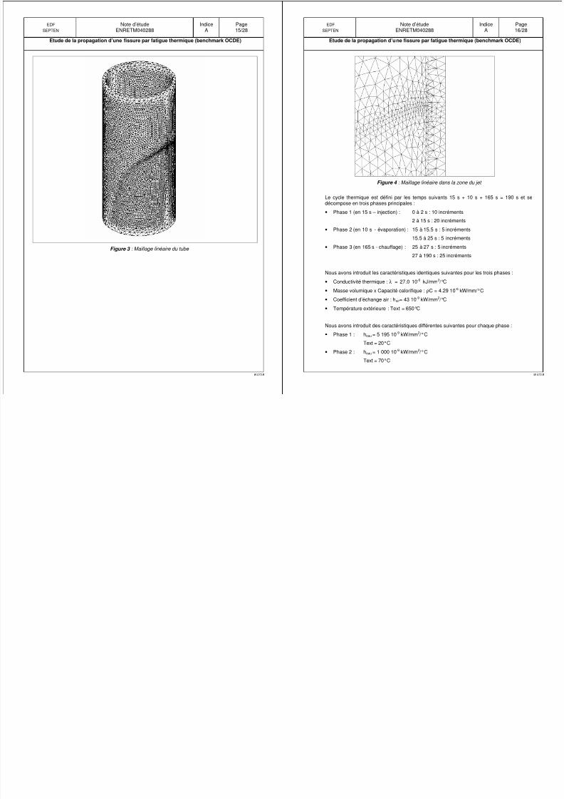
7/31/2019 Nea Study of Thermal Fatigue
http://slidepdf.com/reader/full/nea-study-of-thermal-fatigue 141/147
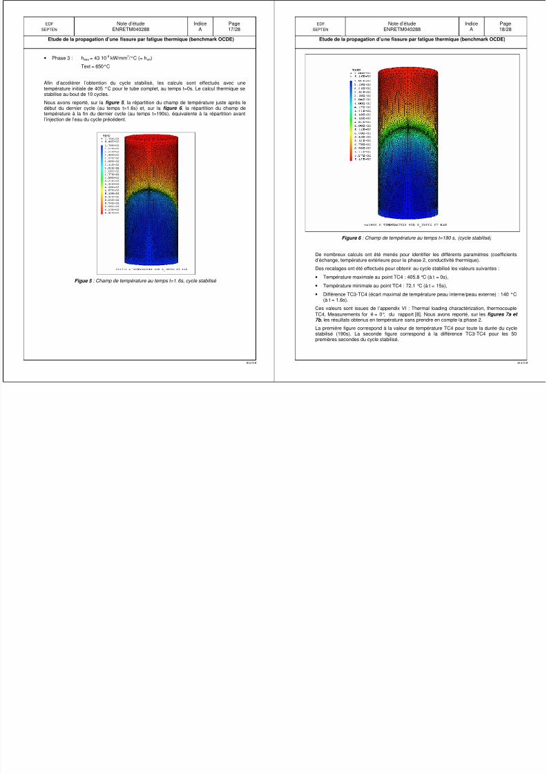
7/31/2019 Nea Study of Thermal Fatigue
http://slidepdf.com/reader/full/nea-study-of-thermal-fatigue 142/147
EDF Note d’étude Indice PageSEPTEN ENRETM040288 A 19/28
Etude de la propagation d’une fissure par fatigue thermique (benchmark OCDE)
Nous remarquons une différence notable entre les résultats numériques et les valeursmesurées pendant les essais. Il est donc nécessaire de prendre en compte la phase 2relative à l’évaporation du film d’eau en surface.Les valeurs de heau et Text de la seconde phase sont déterminées afin d’obtenir les résultatsles plus proches des valeurs expérimentales.
D’autre part, les valeurs heau (1ère phase) et hair ont été obtenues par régression linéaire eneffectuant au préalable des calculs pour des valeurs différentes de ces deux paramètres.Le matériau (acier 316 L) a selon les tables du RCC-M, une conductivité thermique prochede 18 W/m/°C. Nous avons reporté, sur lesfigures 8a et 8b , les résultats en températureobtenus pour cette valeur de conductivité avec la prise en compte des trois phases.La valeur du gradient de température calculée (TC3-TC4), au point maximal de la courbe,est très différente de la valeur mesurée pourλ = 18 W/m/°C.
EDF Note d’étude Indice PageSEPTEN ENRETM040288 A 20/28
Etude de la propagation d’une fissure par fatigue thermique (benchmark OCDE)
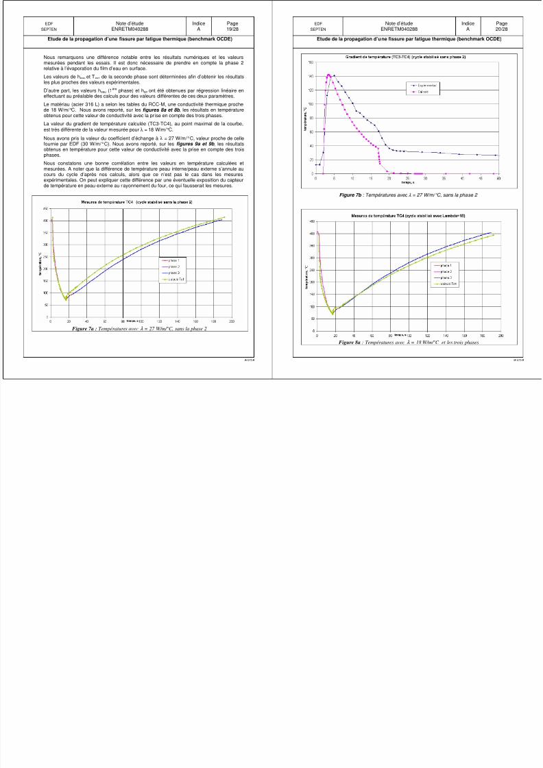
7/31/2019 Nea Study of Thermal Fatigue
http://slidepdf.com/reader/full/nea-study-of-thermal-fatigue 143/147
W 073 B
Nous avons pris la valeur du coefficient d’échange àλ = 27 W/m/°C, valeur proche de cellefournie par EDF (30 W/m/°C). Nous avons reporté, sur lesfigures 9a et 9b , les résultatsobtenus en température pour cette valeur de conductivité avec la prise en compte des trois
phases.Nous constatons une bonne corrélation entre les valeurs en température calculées etmesurées. A noter que la différence de température peau interne/peau externe s’annule aucours du cycle d’après nos calculs, alors que ce n’est pas le cas dans les mesuresexpérimentales. On peut expliquer cette différence par une éventuelle exposition du capteurde température en peau externe au rayonnement du four, ce qui fausserait les mesures.
Figure 7a : Températures avec λ = 27 W/m/°C, sans la phase 2
W 073 B
Figure 7b : Températures avec λ = 27 W/m/°C, sans la phase 2
Figure 8a : Températures avec λ = 18 W/m/°C et les trois phases
EDF Note d’étude Indice PageSEPTEN ENRETM040288 A 21/28
Etude de la propagation d’une fissure par fatigue thermique (benchmark OCDE)
EDF Note d’étude Indice PageSEPTEN ENRETM040288 A 22/28
Etude de la propagation d’une fissure par fatigue thermique (benchmark OCDE)
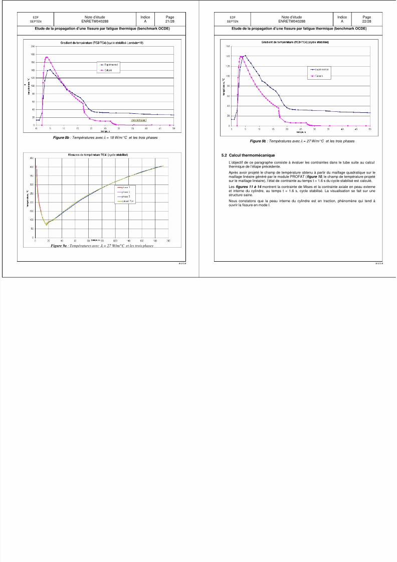
7/31/2019 Nea Study of Thermal Fatigue
http://slidepdf.com/reader/full/nea-study-of-thermal-fatigue 144/147
W 073 B
Figure 8b : Températures avec λ = 18 W/m/°C et les trois phases
Figure 9a : Températures avec λ = 27 W/m/°C et les trois phases
W 073 B
Figure 9b : Températures avec λ = 27 W/m/°C et les trois phases
5.2 Calcul thermomécanique
L’objectif de ce paragraphe consiste à évaluer les contraintes dans le tube suite au calculthermique de l’étape précédente.Après avoir projeté le champ de température obtenu à partir du maillage quadratique sur lemaillage linéaire généré par le module PROFAT (figure 10 , le champ de température projetésur le maillage linéaire), l’état de contrainte au temps t = 1.6 s du cycle stabilisé est calculé.Les figures 11 à 14 montrent la contrainte de Mises et la contrainte axiale en peau externeet interne du cylindre, au temps t = 1.6 s, cycle stabilisé. La visualisation se fait sur unestructure saine.Nous constatons que la peau interne du cylindre est en traction, phénomène qui tend àouvrir la fissure en mode I.
EDF Note d’étude Indice PageSEPTEN ENRETM040288 A 23/28
Etude de la propagation d’une fissure par fatigue thermique (benchmark OCDE)
EDF Note d’étude Indice PageSEPTEN ENRETM040288 A 24/28
Etude de la propagation d’une fissure par fatigue thermique (benchmark OCDE)
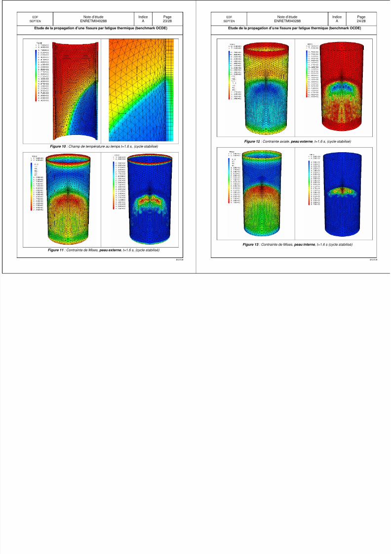
7/31/2019 Nea Study of Thermal Fatigue
http://slidepdf.com/reader/full/nea-study-of-thermal-fatigue 145/147
W 073 B
Figure 10 : Champ de température au temps t=1.6 s, (cycle stabilisé)
Figure 11 : Contrainte de Mises, peau externe , t=1.6 s, (cycle stabilisé)
W 073 B
Figure 12 : Contrainte axiale, peau externe , t=1.6 s, (cycle stabilisé)
Figure 13 : Contrainte de Mises, peau interne , t=1.6 s (cycle stabilisé)
EDF Note d’étude Indice PageSEPTEN ENRETM040288 A 25/28
Etude de la propagation d’une fissure par fatigue thermique (benchmark OCDE)
EDF Note d’étude Indice PageSEPTEN ENRETM040288 A 26/28
Etude de la propagation d’une fissure par fatigue thermique (benchmark OCDE)
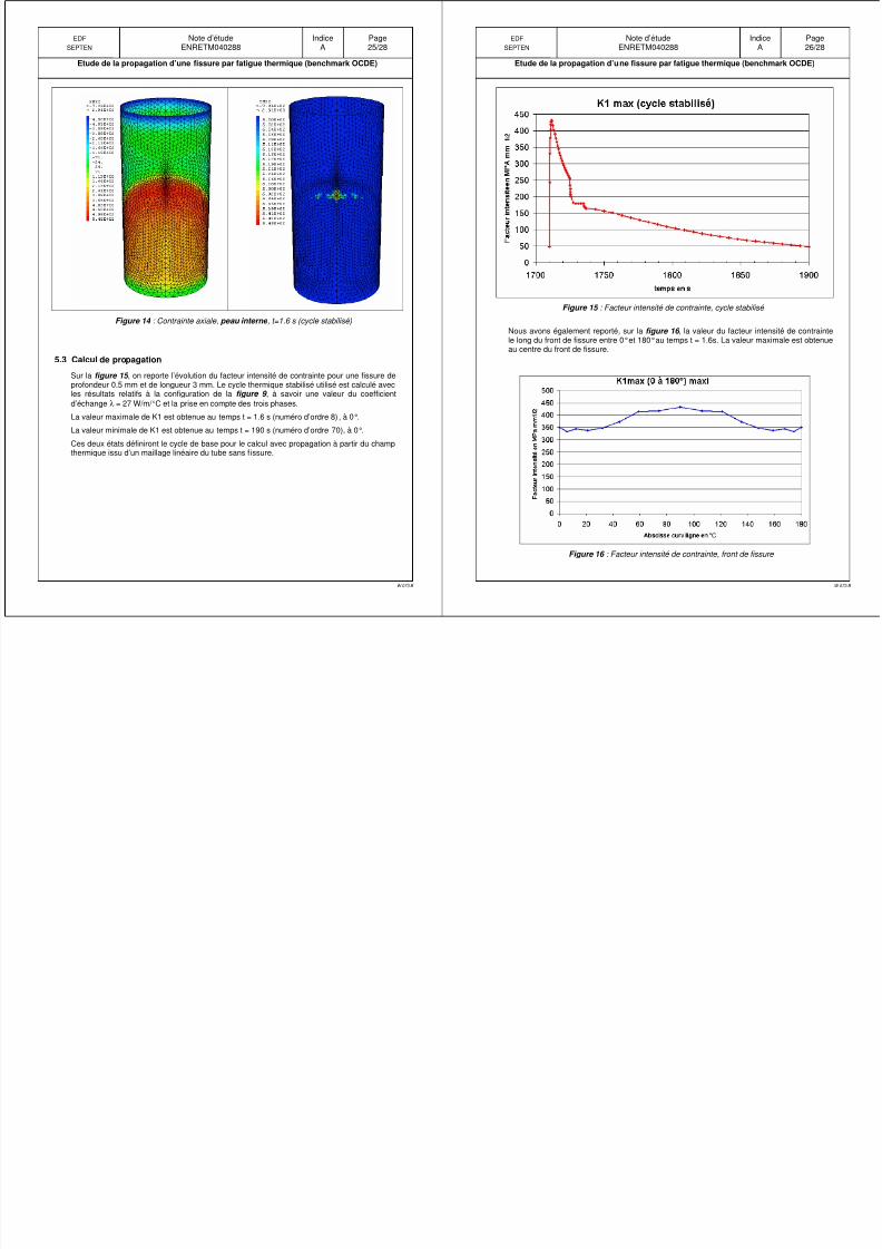
7/31/2019 Nea Study of Thermal Fatigue
http://slidepdf.com/reader/full/nea-study-of-thermal-fatigue 146/147
W 073 B
Figure 14 : Contrainte axiale, peau interne , t=1.6 s (cycle stabilisé)
5.3 Calcul de propagationSur la figure 15 , on reporte l’évolution du facteur intensité de contrainte pour une fissure deprofondeur 0.5 mm et de longueur 3 mm. Le cycle thermique stabilisé utilisé est calculé avecles résultats relatifs à la configuration de lafigure 9 , à savoir une valeur du coefficientd’échangeλ = 27 W/m/°C et la prise en compte des trois phases.La valeur maximale de K1 est obtenue au temps t = 1.6 s (numéro d’ordre 8), à 0°.La valeur minimale de K1 est obtenue au temps t = 190 s (numéro d’ordre 70), à 0°.Ces deux états définiront le cycle de base pour le calcul avec propagation à partir du champthermique issu d’un maillage linéaire du tube sans fissure.
W 073 B
Figure 15 : Facteur intensité de contrainte, cycle stabilisé
Nous avons également reporté, sur lafigure 16 , la valeur du facteur intensité de contraintele long du front de fissure entre 0°et 180°au temps t = 1.6s. La valeur maximale est obtenueau centre du front de fissure.
Figure 16 : Facteur intensité de contrainte, front de fissure
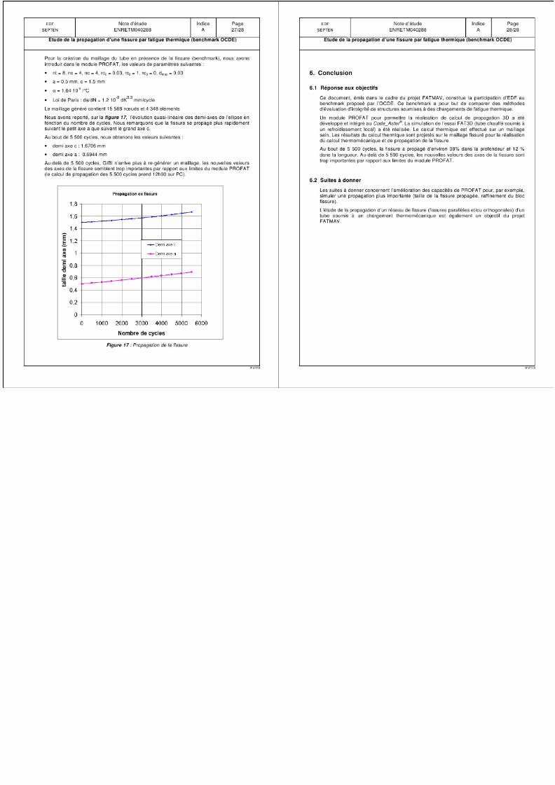
7/31/2019 Nea Study of Thermal Fatigue
http://slidepdf.com/reader/full/nea-study-of-thermal-fatigue 147/147