NEAR EAST UNIVERSITY

FACULTY OF ENGINEERINGMECHANICAL ENGINEERING

DEPARTMENT

ME400INTERNAL FLUID FLOW;

FLOW IN PIPES

STUDENT: ERHAN SELÇUK (971401)

SUPERVISOR: ASSIST. PROF. DR. GÜNER ÖZMEN

•

•NICOSIA 2003

.!..._9_~ıı..-11L1_•_.I_LI_. •-••- ..•~•-•--I• "!!_la

ACKNOWLEDGEMENT

I would like to thank my supervisor Assist. Prof Dr. Güner ÖZMEN her invaluableadvice and belief in my work and myselfover the course of this Graduation Project.

I would like to express my gratitude to Prof. Dr. Kaşif Onaran the chairman of themechanical engineering faculty for his support and advice during educational years inthe university.

I thank my family for their constant encouragement, support and patient to makepossible this thesis during my university life.

I would also like to thank Cem IŞIK, Özgür İNGÜN and Orçun BECAN for theiradvice and support.

•

ABSTRACT

In this project fluid flow in pipes are described in four chapters, each chapter is

introduced common properties and their application.

The first chapter is described fluid properties and definations scope of fluid mechanics,

difference between liquid and gases, viscosity and at the end of the chapter Bernoulli'sequation.

Second chapter is described laminar and turbulent flow phenomena, importance of

viscosity in the laminar and turbulent flow, the role of entrance effects in the flow.

However the types of flow such as internal, extarnal flow are discussed

In the third chapter one and two dimensional flows and specificationsof these flows are

considered. Also Reynolds number laminar, turbulent flows, Reynolds number situation

between these flows, critical Reynolds number critic levels of laminar and turbulentflows are considered.

In the last chapter the types of pipe line system which effect the energy losses and

efficiency are discussed. Energy losses such as minor and friction losses in turbulent

flow that effect efficiency directly are included. Also using of Moddy diagram which is

used to determine friction factor are considered.

ii

TABLE OF CONTENTS

ACKNOWLEDGEMENT................................................................. ı

ABSTRACT.................................................................................. ıı

CHAPTER 1 INTRODUCTION

1.1 FLUID PROPERTIES AND DEFINITIONS 1

1.2 HISTORICAL NOTES 1

1.3 SCOPE OF FLUID MECHANICS 2

1.4 DIMENSIONS AND UNITS 3

1.5 DIFFERENCE BETWEEN LIQUIDS AND GASES .4

1 .6 VISCOSITY 5

1 .6. 1 Dynamic Viscosity 5

1 . 6.2 Kinematic Viscosity 7

1.7 BERNOULLI'S EQUATION 8

1.7.1 Application of Bernoulli's Equation 10

SUMMARY 11

CHAPTER 2 FLOW IN CLOSED CONDUITS

INTRODUCTION 12....

2. 1 LAMINAR AND TURBULENT 12

2.2 EFFECT OF VISCOSITY ···························~····· 17

2.3 ENTRANCE EFFECTS , 19

2.4 INTERNAL AND EXTERNAL FLOWS 21

SUMMARY 23

•

CHAPTER 3 FOUNDATIONS OF FLOW ANALYSIS

INTRODUCTION 24

3.1 ONE AND TWO DIMENSIONAL FLOWS 24

3.2 REYNOLDS NUMBER...•............................................................. 26

3.2.1 Critical Reynolds Number 283.3 REYNOLDS NUMBER FOR CLOSED NONCIRCULAR

CROSS SECTION 30

SUMMARY , 31

CHAPTER 4 PIPE SYSTEMS AND LOSSES

INTRODUCTION 32

4.1 PIPE LINE SYSTEMS 32

4.1.1 Pipes in Series 32

4.1.2 Pipes in Parallel. 33

4.2 MINOR LOSSES 34

4.2.1 Sudden Enlargement 35

4.3 FRICTION LOSS IN TURBULENT FLOW 39

4.3.1 Use ofThe Moody Diagram 45

SUMMARY 48

CONCLUSION ····"···························· 49REFFERENCES............................................................................. 50

CHAPTERl

INTRODUCTION

1.lFLUID PROPERTIES AND DEFINITIONS

Fluid mechanics is the science of the liquid and is based on the same fundamental

princi~lesthat are employed in the mechanics.

Fluid mechanicsmay be divided into 3 branches;

.Fluid Statics

.FluidKinematics

.Fluid Dynamics

Fluid Statics: Is the study of the mechanicsof fluids at rest.

Fluid Kinematics: Deals with velocity and stream lines without considering forces or

energy.

Fluid Dynamics: Is concered with the relation between velocities and acceleration

forces.

1.2 HISTÖRICAL NOTES

Until the turn of this century the study of fluids was undertaken essentially by two

groups-hydraulicians and mathematicians. Hydraulicians worked along empirical lines,

while mathematicians concentrated on analytical lines. The vast and often ingenious

experimentation of the former group yielded much information of indispensable value

to the former group yielded much information of indispensable value to the practicing

engineer of the day. However, lacking the generalizing benefits of workable theory,

these

results were of restricted and limitedvalue in novel situations. Mathematicians

meanwhileby not availingthemselvesof experimental information,were forced to

make assumptions so simplifiedas to render their results very often completelyat oddswith reality.

It became clear to such eminent investigators as Reynolds, Froude, Prandlt and von

Karman that the study of fluid must be a blend of theory and experimentation. Such was

the beginning -of the science of fluid mechanics as it is known today. Our modem

research and test facilities employ mathematicians, physicists, engineers and skilled

technicians, who, working in teams, bring both viewpoints in varying degrees to theirwork.

2

1.3 SCOPE OF FLUID MECHANICS

Having defined a fluid and noted the characteristics that distinguish it from a solid, we

might ask the question: 'Why study fluidmechanics?'

Knowledge and understanding of the basic principles and concepts of fluid mechanics

are essential to analyze any system in which a fluid is the working medium. The design

of virtually all means of transportation requires application of principles of fluid

mechanics. Included are aircraft for both subsonic and supersonic flight, ground effect

machines, hovercraft, vertical takeoff and landing aircraft requiring minimum runway

length, surface ships, submarines, ~d automobiles. In recent years automobile

manufacturers have given more consideration to aerodynamic design. This has been true

for sometime for the designers of both racing cars and boats. The design of propulsion

systems for space flight as well as for toy rockets is based on the principles of fluid

mechanics. The collapse of the Tacoma Narrows Bridge in 1940 is evidence of the

possible consequences of neglecting the basic principles of fluid mechanics. It is

commonplace today to perform model studies to determine the aerodynamic forces, and

flow fields around, buildings and structures. These include studies of skyscrapers,

baseball stadiums, smokestacks, and shopping plazas.

1.4 DIMENSIONS AND UNITS"'

The design of all types of fluid machinery includingpumps, fans, blowers, compressors,

and turbines clearly requires knowledge of the basic principles of fluid mechanics.

Lubrication is an application of considerable importance in fluid mechanics. Heating

and ventilating systems for private homes, large office ~uildings, and underground

tunnels, and the design of pipeline systems are further examples of technical problem

areas requiring knowledge of fluid mechanics. The circularity system of the body is

essentially a fluid system. It is not surprising that the design of blood substitutes,

artificial hearts, heart-lung machines, breathing aids, and other such devices must relyon the basic principlesof fluidmechanics.

Even some of our recreational endeavors are directly related to fluid mechanics. The

slicingand hooking of golf balls can be explainedby the principles of fluidmechanics

The list of applications of the principles of fluid mechanics could be extended

considerably. Our main point here is that fluid mechanics is not a subject studied for

purely academic interest; rather, it is a subject with widespread importance both in oureveryday experiences and in modern technology.

Clearly, we cannot hope to consider in detail even a smallpercentage of these and other

specific problems of fluid mechanics. Instead, the purpose of this text is to present the

basic laws and associated physical concepts that provide the basis or starting point inthe analysisof any problem in fluidmechanics.

Consistent units of force mass, length, time and temperature greatly şimplifyproblem

solutions in mechanics.also derivations can be carried out without reference to any

particular consistent system if units are used in a consistent manner. A system of

mechanicsunits is said to be consistent when a unit force causes a unit ITifiSS to undergo

4

a unit acceleration. The international System (SI) hass been adopted in most countiries

and is expected to be adopted in the United States soon. This system has the Newton

(N) as the unit offorce,the kilogram (kg) as the unit of mass,the meter (m) as the unit of

length and the second(s) as the unit of time. With the kilogram meter and second as

defined units the Newton is derived to exactly satisfyNewton's second law ofmation.

1 N= I kg.I m/s2

1.5 DIFFERENCE BETWEEN LIQUIDS AND GASES

When a liquid is held in a container it tends to take the shape of the container, covering

the bottom and sides. The top surface in contact with the atmosphere above it maintains

a uniform level As the container is tipped the liquid tends to pour out; the rate of

pouring is dependent on a property called viscosity, which will be defined later.

When a gas is held in a closed container it tends to expand and completely fill the

container. If the container is opened the gas tends to continue to expand and escapefrom the container.

In addition to these familiar differences between gases and liquids another difference isimportant in the study of fluid mechanics:

• Liquids are only slightlycompressible

• Gases are readily compressible

Compressibility refers to the change in volume of a substance when the pressure on it

changes. These distinctions are sufficientfor most purposes.

1.6 VISCOSITY

1.6.1 Dynamic Viscosity

A fluid has many properties. One important ptoperty is viscosity, which is a measure of

the resistance the fluid has to shear. Because this property arises from the defination of

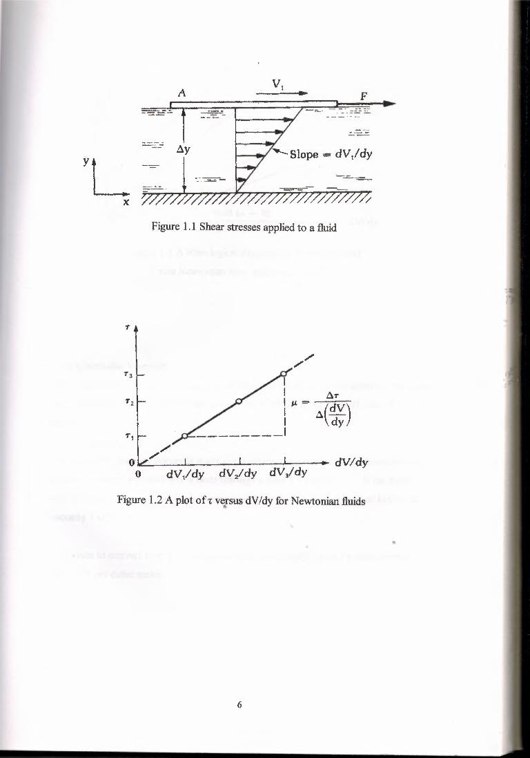
a fluid we will examine it in that regard. Consider again a fluid-filled space formed by

two horizontal parallel plates Figure 1.1. The upper plate has an area A in contact with

the fluid and is pulled to the right with a force F 1 at a velocity V 1. If the velocity at each

point within the fluid could be measured a velocity distribution like that illustrated in

Figure 1. 1 might result. The fluid velocity at the moving plate is V ı because the fluid

adheres to that surface. At the bottom, the velocity is zero with respect to the boundary,

owing to the nonslip condition. The slope of the velocity distribution is dVı/dy.

If this experiment is repeated with F2 as the force a different slope or strain rate results;

dV 2/dy. In general, to each applied force there corresponds only one shear stress and

only one strain rate. If data froı;n the series of these experiments were plotted ast versus

dv/dy, Figure; 1 .2 would result for a fluid like water. The points lie on a straight line that

passes through the origin. The slope of the resulting line in Figure f .2 is the viscosity öf

the fluid because it is a measure of the fluid's resistance to shear. In other words,

viscosity indicates how a fluid will react (dV/dy) under the action of external stress (r)

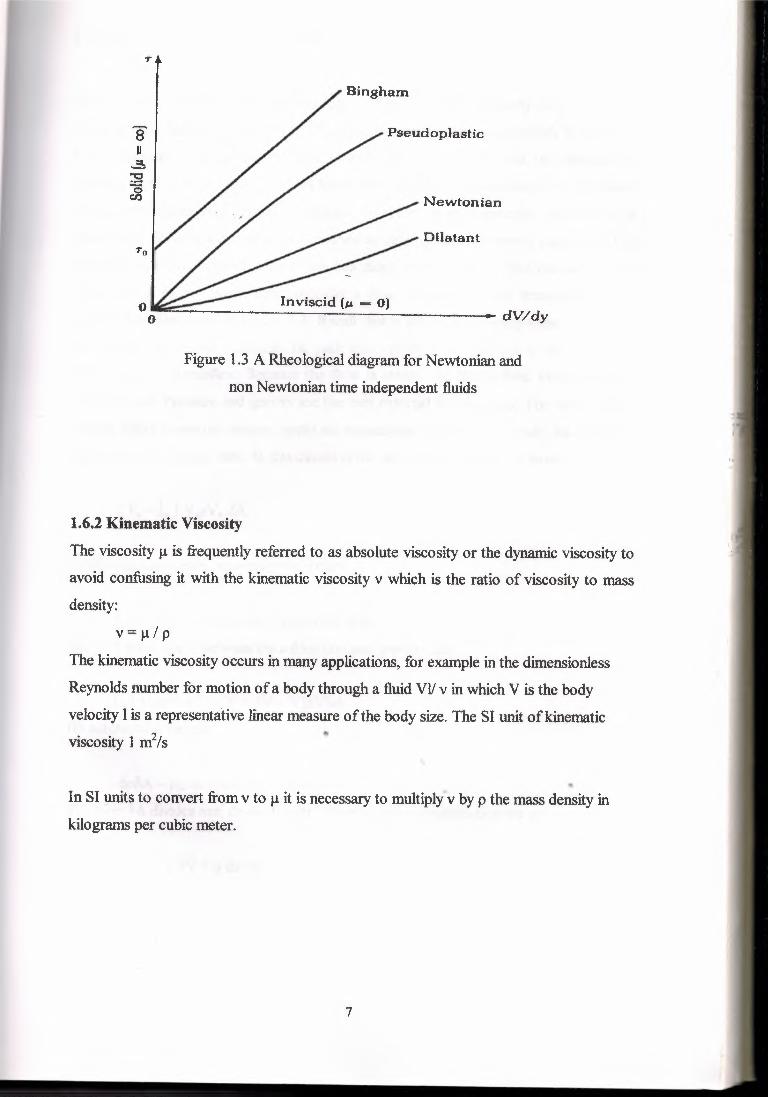
The plot of Figure 1 .2 is a straight line that passes through the origin. This result is

characteristic of a Newtonian fluid, but there are other types of fluids called non­

Newtonian fluids. A graph of r versus dv/dy, called a theological diagram, is shown in

Figure 1.3 for several types of fluids. Newton's law of viscosity and are represented by

the equation, ••

t = µdv/dy

ıı : the, applied shear stress

µ : the absolute or dynamic viscosity of the fluid

dv/dy : the strain rate in dimensions of 1/T

5

A F

X

Figure 1.1 Shear stresses applied to a fluid

T

Tz

II ~T

I µ. = ----(d. V)I ~ dy_ı-------

oI 1

dV2/dy d\13/dy•.. dV/dy

Figure 1,2 A plot of 1versus dV/dy for Newtonian fluids

6

Dilatant

Pseudo plastic

Newtonian

Figure 1.3 A Rheological diagram for Newtonian and

non Newtonian time independent fluids

1.6.2 Kinematic Viscosity

The viscosityµ is frequently referred to as absolute viscosity or the dynamic viscosity to

avoid confusing it with the kinematic viscosity v which is the ratio of viscosity to massdensity:

v= µ/ p

The kinematic viscosity occurs in many applications, for example in the dimensionless

Reynolds number for motion of a body through a fluidVII v in which V is the body

velocity I is a representative linear measure of the body size. The SI unit of kinematicviscosity 1 m2/s

•In SI units to convert from v to µ it is necessary to multiplyv by p the mass density inkilogramsper cubic meter.

7

~dpoA - pg ds oA cos0 = pV dV oA

The term öA divides out; ds cos 0 is dz.Therefore after simplificationwe get•

1.7 BERNOULLI EQUATION

The Bernoulli Equation gives a relationship between pressure, velocity and position or

elevation in a fluid flow field. Normally, these properties vary considerably in the flow

field. Normally these properties vary considerably in the flow and the relationship

between them if written in differential form quite complex. The equations can be solved

exactly only under very special conditions. Therefore in most practical problems jt is

often more convenient to make assumptions to simplify the descriptive equations. The

Bernoulli equation is simplification that has many applications in fluid mechanics. We

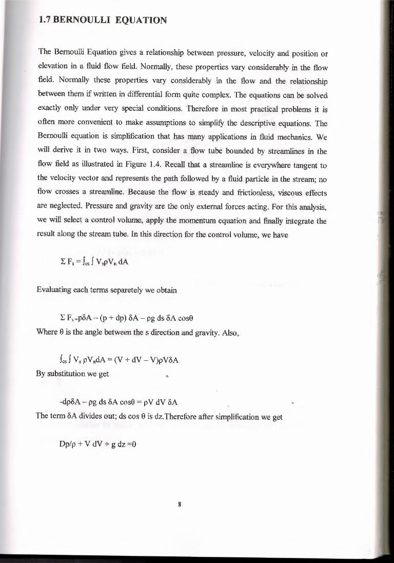
will derive it in two ways. First, consider a flow tube bounded by streamlines in the

flow field as illustrated in Figure i .4. Recall that a streamline is everywhere tangent to

the velocity vector and represents the path followed by a fluid particle in the stream; no

flow crosses a streamline. Because the flow is steady and frictionless, viscous effects

are neglected. Pressure and gravity are the only external forces acting, For this analysis,

we will select a control volume, apply the momentum equation and finally integrate the

result along the stream tube. In this direction for the control volume, we have

Evaluating each terms separetely we obtain

t F~,.,pöA-r- (p + dp) öA- pg ds ÖA cos0

Where 0 is the angle between the s direction and gravity. Also,

fes f VspVndA±:: (V + dV - V)pVôA

By substitution we get

Dp/p + V dV + g dz =O

8

"'

pgdsaA

Figure 1.4 A differential control volume for the derivation of Bernoulli's eq.

Integrating between points 1 and 2 along the stream tube gives

For the special case of an incompressible fluid density is constant (rıot a :function of

pressure ) and the equation then becomes;

v: -v.ıPı-Pı+ 2 ı +g(z2-z,)=0p 2

or

vıP +-2- + gz = a constantp 2

Bernoulli equation for steady incompressible flow along a streamline with no friction(no viscous effects).

9

1.7.1 Application of Bernoulli's Equation

1-) Decide which items are known and what is to be found.

2-) Decide which two sections in the system will be used writing Bernoulli's e~uation.

One section is chosen for which much data is known. The second is usually the

Section at which something is to be calculated.

3-) Write Bernoulli's equation for the two selected sections in the system. It is

important that the equation is written in the direction of flow. That is the flow must

proceed from the section on the left side of the equation to that on the right side.

4-) Simplifythe equation ifpossible by cancellingterms that are zero or those that are

equal ön both sides of the equation.

5-) Solve the equation algebraicallyfor the desired term.

6-) Substitute known quantities and calculate the result, being careful that consistent

units are used throughout the calculations.

•

10

••

SUMMARY

Fluid mechanics is the science of the liquid and is based in three basic branches. They

are fluid statics, fluid kinematics, fluid dynamics. Difference between liquids and gases

are examined as followed. Another important factor is viscosity, which is a measure of

the resistance the fluid has to shear. At the end of the chapter Bernoulli's equation is

determined and also described applications.

11

CHAPTER2

FLOW IN CLOSED CONDUITS

INTRODUCTION

The purpose of this chapter is to descnbe laminar and turbulent flow phenomena,

importance of viscosity in the laminar and turbulent flow, the role of entrance effects in

the flow. However the types of flow such as internal, external flow are discussed.

2.1 LAMINAR AND TURBULENT FLOW

In early experiments with flow in pipes, it was discovered that two different flow

regimes exist- laminar and turbulent. When laminar flow exists in a system. the fluid

flows in smooth layers called laminae. A fluid particle in one layer stays in that layer.

The layers of fluid slide by one another without apparent eddies or swirls. Turbulent

flow, on the other hand, exists at much higher flow rates in the system. In this cage,

eddies and vortices mix the fluid by moving particles tortuously ab out the cross section.

The existence of two types of flow is easily visualized by examining results of

experiments performed by Osborne Reynolds. His apparatus is shown schematically in

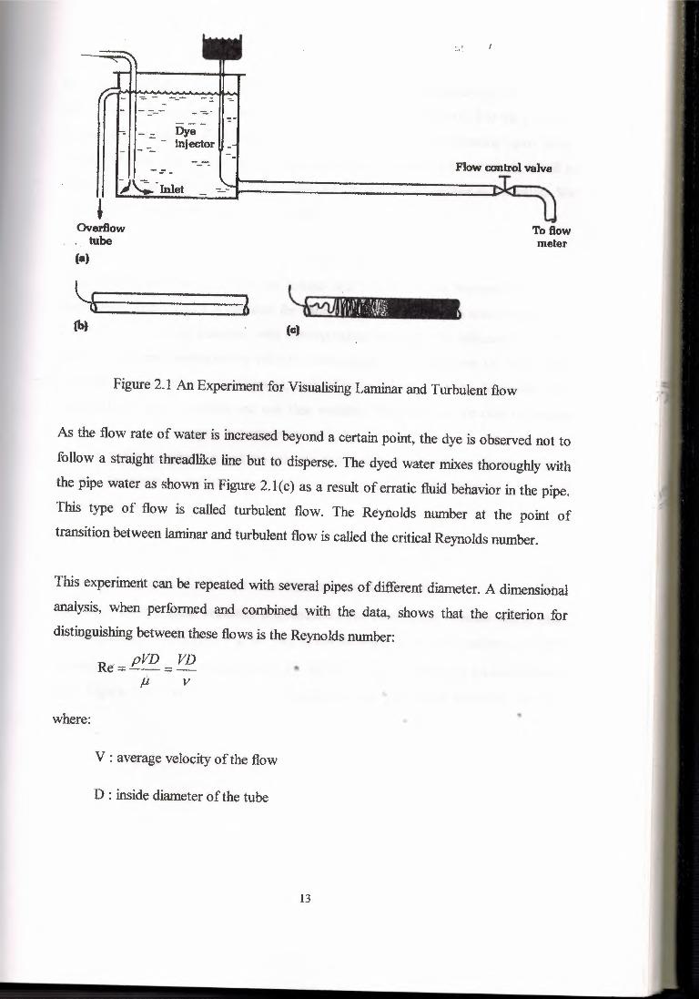
Figure 2.l(a). A transparent tube is attached to a constant-head tank with water as the

liquid medium. The opposite end of the tube has a valve to control the flow rate. Dyed

water is injected into the water at the tube inlet, and the resulting flow pattern is

observed. For low rates of flow; something similar to Figure 2.l(b) results. The dye

pattern is regular and forms a single line like a thread. There is no lateral mixing in any

part of the tube, and the flow follows parallel streamlines. This type of flow is called

laminaror viscous flow.

12

To flowmeter

-ı ı-=.. - --- -;:;

ny-;­- : - injector

Flow control valve

)~·Inlet

'Overflow.. tube(a)

l& ıfbt (c)

Figure 2.1 An Experiment for VisualisingLaminar and Turbulent flow

As the flow rate of water is increased beyond a certain point, the dye is observed not to

follow a straight threadlike line but to disperse. The dyed water tnixes thoroughly with

the pipe water as shown in Figure 2.l(c) as a result of erratic fluid behavior in the pipe.

This type of flow is called turbulent flow. The Reynolds number at the point of

transitionbetween laminarand turbulent flow is called the critical Reynolds number.

This experiment can be repeated with several pipes of different diameter. A dimensional

analysis, when performed and combined with the data, shows that the criterion fordistinguishingbetweeh these flows is the Reynolds number:

Re= pVD = VDjı V

where:

V: average velocity of the flow

D: inside diameter of the tube

13

---------- - ------

For 'straight circular pipes, the flow is always laminar for a Reynolds number less-than

2100. The flow is usually turbulent for Reynolds numbers over 4000. For the transition

regime in between, the flow can be either laminar or turbulent, depending upon details

of the apparatus that cannot always be predicted or controlled. For our work, it will at

times be necessary to have an exact value for the Reynolcls number at transition. We

will arbitrarily choose this value to be 2 100.

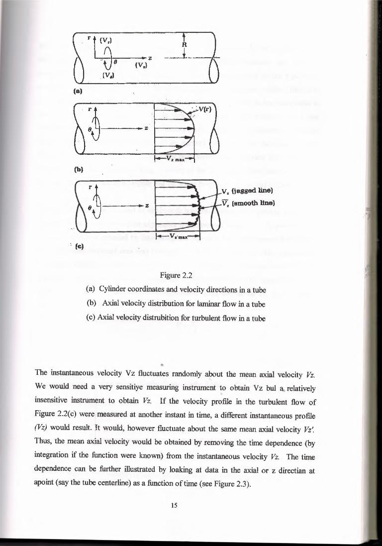
A distinction must be made between laminar and turbulent flows because the velocity

distribution within a duct is different for each. Figure 2,2{a) shows a coordinate system

for flow in a tube, for example, with corresponding velocities. As indicated, there can

be three different İnstantaneous velocity components in a conduit-one for each of the

three principal directions. Furthermore, each of these velocities can be dependent upon

at most three space variables and one time variable. If the flow in the tube is laminar,

we have only one nonzero instantaneous velocity: V.z Moreover, Vz is a function of

only the radial coordinate r, and the velocity distribution is parabolic as shown in Figure

2.2(b ). An equation for this distribution is derivable from the equation of motion

performed Iater in this chapter.

If the flow is turbulent; all three instantaneous velocities Vr, V 11, and Vz are nonzero.

Moreover, each of these velocities is a function of all three space variables and of time.

An equation for velocity(Vr, V11, or Vz) is not derivable from the equation of motion.

Therefore, to envision the axial velocity, for instance, we must rely on experimental

data. Figure 2.2(c) shows the axial instantaneous velocity Vz for turbulent flow in a

tube.

14

rt (V,J

-e. z(Vz}

[V,l

(a)

( :~ \ '.::-i. · : V(r). .,.--z·

(b)

:~ z

Vz (jagged line)

I •\......-.t--V2 [smooth line)

: (c)

Figure 2.2

(a) Cylindercoordinates and velocity directions in a tube

(b) Axial velocity distribution for laminar flow in a tube

(c) Axial velocity distrubition for turbulent flow in a tube

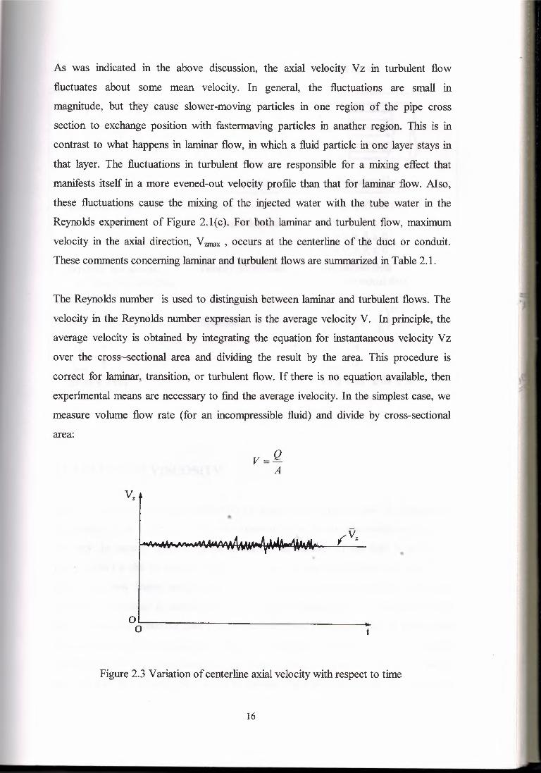
The instantaneous velocity Vz fluctuates randomly about the mean axial velocity Vz.

We would need a very sensitiye measuring instrument to obtain Vz bul a. relatively

insensitive instrument to obtain Vz. If the velocity profile in the turbulent flow of

Figure 2.2(c) were measured at another instant in time, a different instantaneous profile

(Vz) would result. It would, however fluctuate about the same mean axial velocity Vz'.

Thus, the mean axial velocity would be obtained by removing the time dependence (by

integration if the function were known) from the instantaneous velocity Vz. The time

dependence can be further illustrated by loaking at data in the axial or z directian at

apoint (say the tube centerline) as a function of time (see Figure 2.3).

15

•

As was indicated in the above discussion, the axial velocity Vz in turbulent flow

fluctuates about some mean velocity. In general, the fluctuations are small in

magnitude, but they cause slower-moving particles in one region of the pipe cross

section to exchange position with fastermaving particles in anather region. This is in

contrast to what happens in laminar flow, in which a fluid particle in one layer stays in

that layer. The fluctuations in turbulent flow are responsible for a mixing effect that

manifests itself in a more evened-out velocity profile than that for laminar flow. Also,

these fluctuations cause the mixing of the injected water with the tube water in the

Reynolds experiment of Figure 2.l(c). For both laminar and turbulent flow, maximum

velocity in the axial direction, Vzmax , occurs at the centerline of the duct or conduit.

These comments concerning laminar and turbulent flows are summarized in Table 2.1.

The Reynolds number is used to distinguishbetween laminar and turbulent flows, The

velocity in the Reynolds number expressian is the average velocity V. Ip principle, the

average velocity is obtained by integrating the equation for instantaneous velocity Vz

over the cross-sectional area and dividing the result by the area. This procedure is

correct for laminar, transition, or turbulent flow. If there is no equation available, then

experimental means are necessary to find the average ivelocity. In the simplest case, we

measure volume flow rate (for an incompressible fluid) and divide by cross-sectional

area:

Figure 2.3 Variation of Centerlineaxial velocity with respect to time

16

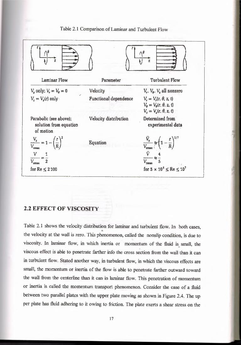
Table 2.1 Comparison of Laminar and Turbulent Flow

Laminar Flow Parameter Turbulent Flow

V1only; V, = Ve = oV: = V,(r) only,

Parabolic (see above);solution from equationof motion

l=1-(!..)2Vmıaıı RV 1

Vımu =2for Re S 2100

VelocityFunctional dependence

V,, V9, V. all nonzeroV, = V,(r, (J, Z, t)v, = V,(r, e. Z, t)vı = V,(r, 8, Z, tJDetermined from

experimental dataVelocity distribution

Equation Yr ~ .r)t/7- 1-:-v,max ı Rv 4~~-

Y:ınax 5 .for 5 x 105 S Re s 10 7

2.2 EFFECT OF VISCOSITY

Table 2.1 shows the velocity distribution for laminar and turbulent flow. In both cases,~

the velocity at the wall is zero. This phenomenon, called the nonslip condition, is due to

viscosity. In laminar flow, in which inertia or momentum of the fluid. is~ small, the

viscous effect is able to penetrate farther info the cross section from the wall than it can

in turbulent flow. Stated another way, in turbulent flow, in which the viscous effects are

small, the momentum or inertia of the flow is able to penetrate farther outward toward

the wall from the centerline than it can in laminar flow. This penetration of momentum

or inertia is called the momentum transport phenomenon. Consider the case of a fluid

between two parallel plates with the upper plate moving as shown in Figure 2.4. The Up

per plate has fluid adhering to it owing to friction. The plate exerts a shear stress on the

17

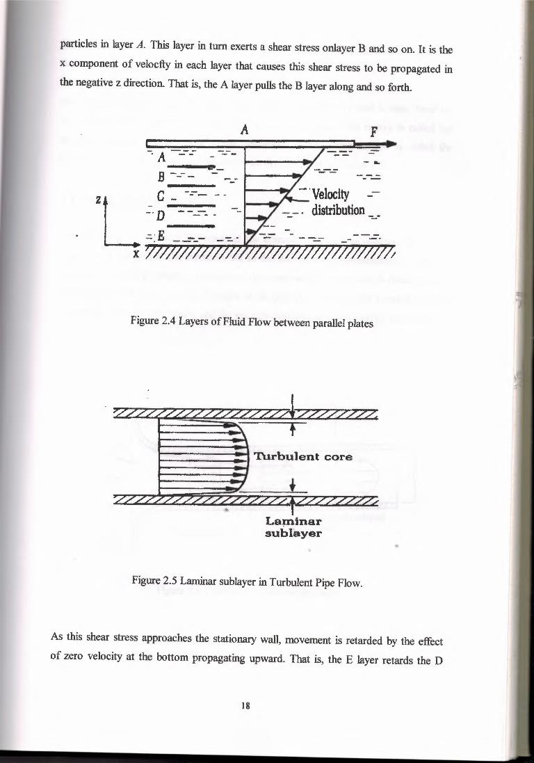
particles in layer A. This layer in tum exerts a shear stress onlayer Band so on. It is the

x component of velocfty in each layer that causes this shear stress to be propagated in

the negative z direction. That is, the A layer pulls the B layer along and so forth.

A F

B ----zL :·~-- -.:: . E

-. A ---- - - ..

X

Laminarsublayer

Figure 2.4 Layers of Fluid Flow between parallel plates

Figure 2.5 Laminar sublayer in Turbulent Pipe Flow.

As this shear stress approaches the stationary wall, movement is retarded by the effect

of zero velocity at the bottom propagating upward. That is, the E layer retards the D

18

••

layer and so on. The resultant effect on velocity is the distribution sketchedin Figure 2.4

As we saw earlier, in turbulent flow, the velocity at a stationary wall is zero. Near the

wall, then, there must be a region of now that is laminar. This region is called the

laminar sublayer, and the now in the remainder of the cross section is called the

turbulent core. Both regions are illustrated for now in a pipe in Figure 2.5.

2.3 ENTRANCE EFFECTS

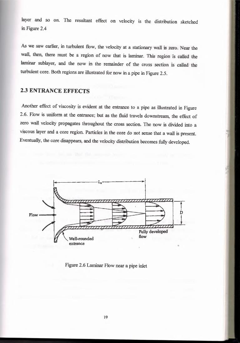
Another effect of viscosity is evident at the entrance to a pipe as illustrated in Figure

2.6. Flow is uniform at the entrance; but as the fluid travels downstream, the effect of

zero wall velocity propagates throughout the cross section. The now is divided into a

viscous layer and a core region. Particles in the core do not sense that a wall is present.

Eventually, the core disappears, and the velocity distribution becomes fullydeveloped.

tDı6zm'ziiizzzzzıızE2z>zzzzzzız)z'Z??zzzzA

n.n •.,ı_.,,.1.•.•~

\ Well-roundedentrance

Figure 2.6 Laminar Flow near a pipe inlet

19

The distance Le Figure 2.6 is called the entrance length, and its magnitude is dependent

upon the forces of inertia and viscosity. It has been determined from numerous

experimental and analytical investigations that the entrance length can be estimatedwith;

Le = 0.06D(Re) (Laminar flow)

Le= 4.4D(Re/16 (Turbulent flow)

Where;

Re= pVD = VDµ V

For laminar flow, we see that the entrance length varies directly with the Reynolds

number. The largest Reynolds number encountered in laminar flow is 2100.

Le= 0.060(2100) = 1260

Thus, l 26 diameters is the maximum length that would be required for fully developedconditions to exist in laminar flow.

For turbulent now, the entrance length varies with the 1/6 power of the Reynolds

number. Conceptually, there is no upper limit for the Reynolds number in turbulent

flow, but in many engineering applications, 104 < Re < 106• Over this range, wecalculate equation turbulent flow.

So in turbulent flow, the entrance length varies to values that are considerably less than

the 126 diameters required at a Reynolds number of 2100. The reason that a shorter

length is required in turbulent flow is the mixing action. For abrupt or sharp-edged

20

number; for laminar flow Langhaar [2] developed the theoretical formula; "'

entrances, additional turbulence is created at the inlet. The effect is to decreas the inletlength required for fullydeveloped flow to exist.

2.4 INTERNAL AND EXTERNAL FLOWS

Another method of categorizing flows is by examining the geometry of the flow field.

Internal flow involves flow in a bounded zegion, as the name implies. External flow

involves fluid in an unbounded region in which the focus of attention is on the flowpattern around a body immersed in the fluid.

The motion of a real fluid is influenced significantlyby the presence of the boundary.

Fluid particles at the wall remain at rest in contact with the wall. In the flow field a

strong velocity gradient exists in the vicinity of the wall, a region referred to as the

boundary layer. A retarding shear force is applied to the fluid at the wall, the boundarylayer being a region of significantshear stresses,

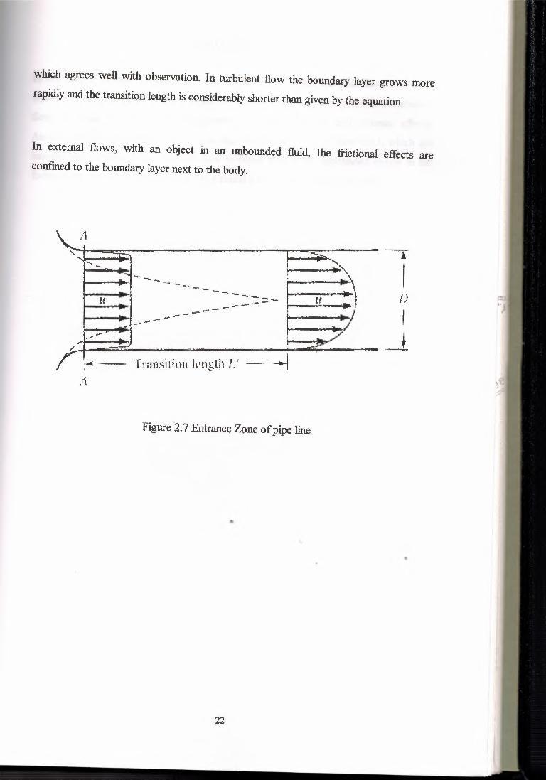
This chapter deals with flows constrained by walls in which the boundary effect is

likely to extend through the entire flow. The boundary influence is easily visualized at

the entrance to a pipe from a reservoir, seen in Fig. 2. 7 At section A-A, near a o well­

rounded entrance, the velocity profile is almost uniform over the cross section. The

action 'of the wall shearing stress is to slow down the fluid near the wall. As a

consequence of continuity, the velocity must increase in the central region. Beyond a

transitional length L ' the velocity profile is fixed since the boundary influence has

extended to the pipe center line. The transition length is a function of the Reynolds

£_ = 0,058RD

21

22

which agrees well with observation. In turbulent flow the boundary layer grows more

rapidly and the transition length is considerably shorter than given by the equation.

In external flows, with an object in an unbounded fluid, the frictional effects areconfined to the boundary layer next to the body.

I)

I~f-:.;::!;} L ::r::::: .-1

Transuiou knflh I,' - ......••..j....• _A

Figure 2.7- Entrance Zone ofpipe line

•

SUMMARY

In this chapter laminar and turbulent flow are described. When the fluid flows in smooth

layers it is laminar flow, if much higher flow rates existed in the system it is turbulent

flow. According to the fluid are examined effect of viscosity and entrance effects.

Another categorizing flows are by exarninig the geometry of the flow field, which are

internal and external flows. Internal flow involved flow in an unbounded region in the

focus of attention is on the flow pattern a round a body immersed in the fluids.

23

24

CHAPTER3

FOUNDATIONS OF FLOW ANALYSIS

INTRODUCTJON

In this chapter one and two dimensional flows and specifications of these flows are

considered. Also Reynolds Number laminar, turbulent flows , Reynolds number

situation between these flows , critical Reynolds Number critic levels of laminar andturbulent flows are considered.

3.1 ONE AND TWO-DIMENSIONAL FLOWS

In every analysis a hypothetical substance or process is set forth which lends itself to

mathematical treatment while still yielding results of pratical value. We have already

discussed the continuum concept. Now, simplifiedflows are set forth, which, when used

with discretion, will permit the use .of higly developed theory on problems ofengineering interest.

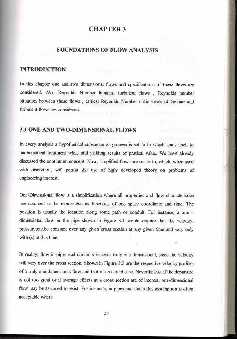
One-Dimensional flow is a simplificationwhere all properties and flow characteristics

are assumed to be expressible as functions of one space coordinate and time. The

position is usually the location along some path or conduit. For instance, a one -

dimensional flow in the pipe shown in Figure 3.1 would require that the velocity,••pressure,etc.be constant over any given cross section at any given time and vary only

with (s) at this time.

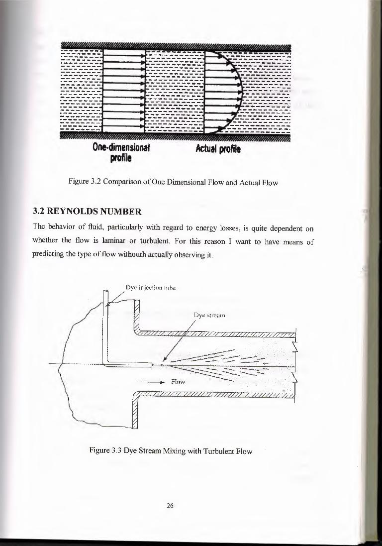
In reality, flow in pipes and conduits is never truly one dimensional, since the velocity

will vary over the cross section, Shown in Figure 3.2 are the respective velocity profiles

of a truly one-dimensional flow and that of an actual case. Nevertheless, if the departure

is not too great or if avarage effects at a cross sectien are of interest, one-dimensional

flow may be assumed to exist. For instance, in pipes and ducts this assumption is often

acceptable where

• Variation of cross section of the container is not too excessive.

• Curvature of the streamlines is not excessive.

• Velocity profile is known not to change appreciablyalong the duct.

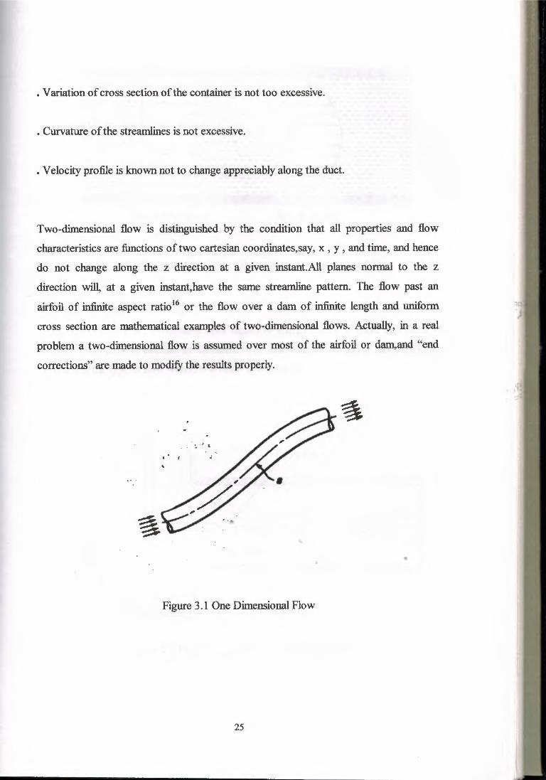
Two-dimensional flow is distinguished by the condition that all properties and flow

characteristics are functions of two cartesian coordinates,say, x , y , and time, and hence

do not change along the z direction at a given instant.All planes normal to the z

direction will, at a given instant,have the same streamline pattern. The flow past an

airfoil of infinite aspect ratio16 or the flow over a dam of infinite length and uniform

cross section are mathematical examples of two-dimensional flows. Actually, in a real

problem a two-dimensional flow is assumed over most of the airfoil or dam,and "end

corrections" are made to modify the results properly.

Figure 3.1 One DimensionalFlow

25

One-dimensionalprofile

Actual profift

Figure 3.2 Comparison of One DimensionalFlow and Actual Flow

3.2 REYNOLDS NUMBER

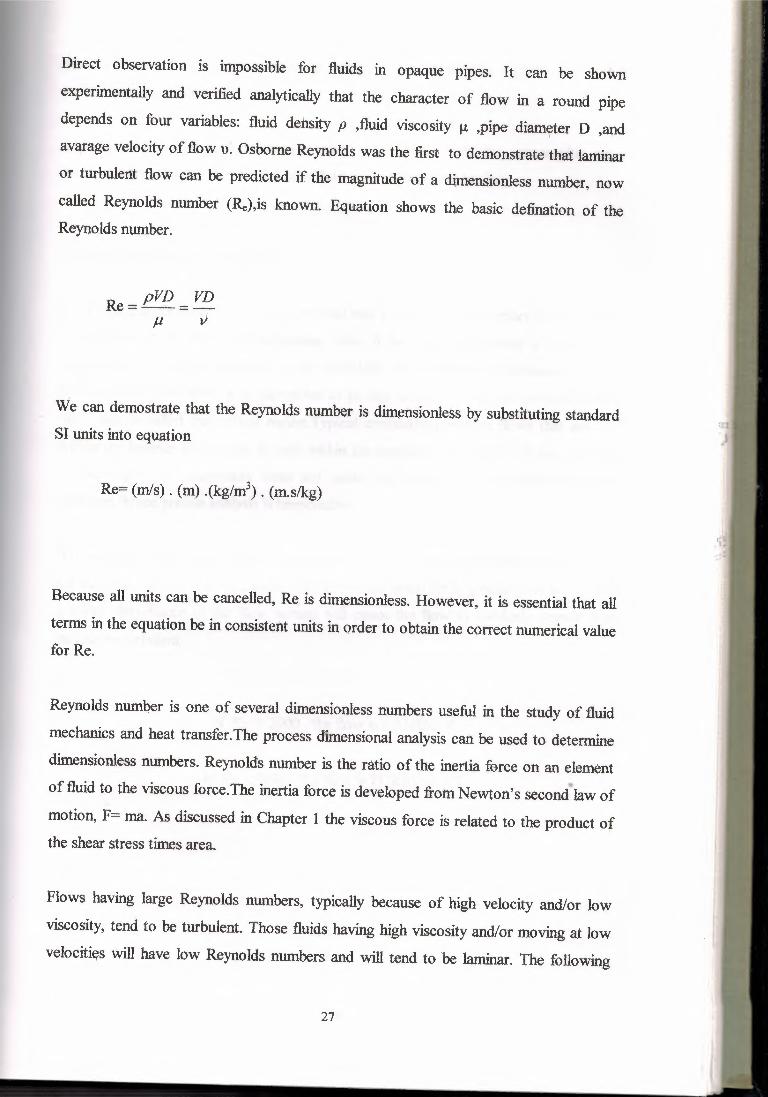
The behavior of fluid, particularly 'with regard to energy losses, is quite dependent on

whether the flow is laminar or turbulent. For this reason I want to have means of

predicting the type of flow withouth actually observing it.

Dye inject ion ı uhe

Figure 3.3 Dye Stream Mixingwith Turbulent Flow

26

27

Direct observation is impossible for fluids in opaque pipes. It can be shown

experimentally and verified analytically that the character of flow in a round pipe

depends on four variables: fluid density p .fhıid viscosity µ ,pipe diameter D .and

avarage velocity of flow u, Osborne Reynolds was the first to demonstrate that laminar

or turbulent flow can be predicted if the magnitude -of a dimensionless number, now

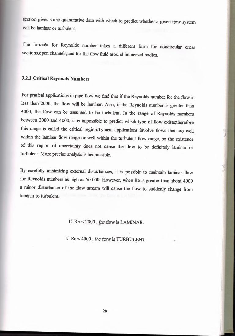
called Reynolds number (Re),is known. Equation shows the basic defination of theReynolds number.

Re= pVD _ VD--µ v

We can demostrate that the Reynolds number is dimensionlessby substituting standardSI units into equation

Re= (mis) . ün) .(kg/m3) • (m.s/kg)

Because all units can be cancelled, Re is dimensionless. However, it is essential that all

terms in the equation be in consistent units in order to obtain the correct numerical valuefor Re.

Reynolds number is one of several dimensionless numbers useful in the study of fluid

mechanics and heat transfer.The process dimensional analysis can be used to determine

dimensionless numbers. Reynolds number is the ratio of the inertia force on an element

of fluid to the viscous force.The inertia force is developed from Newton's second law of

motion, F= ma. As discussed in Chapter I the viscous force is related to the product ofthe shear stress times area.

Flows having large Reynolds numbers, typically because of high velocity and/or low

viscosity, tend to be turbulent. Those fluids having high viscosity and/or moving at low

velocities will have low Reynolds numbers and will tend to be laminar. The following

28

section gives some quantitative data with which to predict whether a given flow systemwill be laminaror turbulent.

The formula for Reynolds number takes a different form for noncircular crosssections,open channels,and for the flow fluid around immersedbodies.

3.2.1 Critical Reynolds Numbers

For pratical applications in pipe flow we find that if the Reynolds number for the flow is

less than 2000, the flow will be laminar. Also, if the Reynolds number is greater than

4000, the flow can be assumed to be turbulent. In the range of Reynolds numbers

between 2000 and 4000, it is impossible to predict which type of flow exists;therefore

this range is called the critical region.Typical applications involve flows that are well

within the laminar flow range or well within the turbulent flow range, so the existence

of this region of uncertainty does not cause the flow to be definitely laminar orturbulent. More precise analysis is henpossible.

By carefully minimizing external disturbances, it is possible to maintain laminar flow

for Reynolds numbers as high as 50 000. However, when Re is greater than about 4000

a minor disturbance of the flow stream will cause the flow to suddenly change fromlaminar to turbulent.

If Re < 2000 , the flow is LAMİNAR.

If Re< 4000 , the flow is TURBULENT.•

••

Examnle Problem: Determine whether the flow is laminar or turbulent if glycerine at

25°C flows in a pipe with a 150-ınm inside diameter.The avarage velocity of flow is 3.6mis.

Solution We must firs evaluate the Reynolds number using Equation

Re= uDp/µ

Where;

u = 3.6 mis

D=0.15m

p = 1258 kg/m'

µ = 9.60 xlO -ı Pa .s

Than we have

Re= (3.6Xo.ısX1258) = 7089.60xıo-ı

Because Re= 708 which less than 2000, the flow is LAMİNAR.

29

3.3 REYNOLDS NUMBER ,FOR CLOSED NON CIRCULAR

CROSS SECTION

When the fluid completely fills the available cross-sectional area and is under pressure ,

the average velocity of flow is determined by using the volume flow rate and the net

flow area in the familiar continuity equation. That is note that the area is the same as

that used to compute the hydraulic radius.

u=Q/A

The Reynolds number for flow in noncircular sections is computed in a very similar

manner to that used for circular pipes and tubes. The only alteration to Reynolds

number equation is replacement of the diameter D with 4R, four times the hydraulic

radius. The results is;

Re= v(4R)p = v(4R)µ V

The validity of this substitution can be demonstrated by calculating the hydraulic radius

for a circular pipe;

R = ~ = mJ2 14 = DWP 1tD 4

Then; D=4R

Therefore 4R is equivalent to D for the circular pipe. Thus, by analogy the use of 4R as

the characteristic dimension for noneirçular cross sections is appropriate. This approach

will give reasonable results as long as the cross section has anaspect ratio not much

different from that of the circular cross section. In this. context aspect ratio is the ratio of

the width of the section to its height. So for a circular section the aspect ratio is I.O

30

SUMMARY

In the third chapter is considered one and two dimensionalflows and Reynolds number.

Reynolds number is one of several dimensionless numbers useful in the study of fluid

mechanics and heat transfer. Reynolds number is the ratio of the inertia force on an

element of fluid to the viscous force. If the Reynolds number is less than 2000 the flow

is laminar. Also, ıf the Reynols number is greater than 4000 the flow is turbulent. The

range ofReynols number is between 2000 and 4000, is called critical region.

31

l

CHAPTER4

PIPE SYSTEMS AND LOSSES

INTRODUCTION

In this section the types of pipe line system which effect the energy losses and

efficiency are discussed. Energy losses such as minor and friction losses in turbulent

flow that effect efficiency directly are included. Also using of Moddy diagram which isused to determine friction factor are considered.

4.1 PIPE LINE SYSTEMS

4.1.1 Pipes In Series

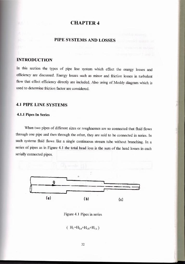
When two pipes of different sizes or roughnesses are so connected that fluid flows

through one pipe and then through the other, they are said to be connected in series. In

such systems fluid flows like a single continuous stream tube without branching. In a

series of pipes as in Figure 4. 1 the total head loss is the sum of the head losses in eachseriallyconnected pipes.

(o) ( b) (e)

E- L

L.- ·--~~---~·-3___ r

Figure 4. 1 Pipes in series

32

4.1.2 Pipes In Parallel

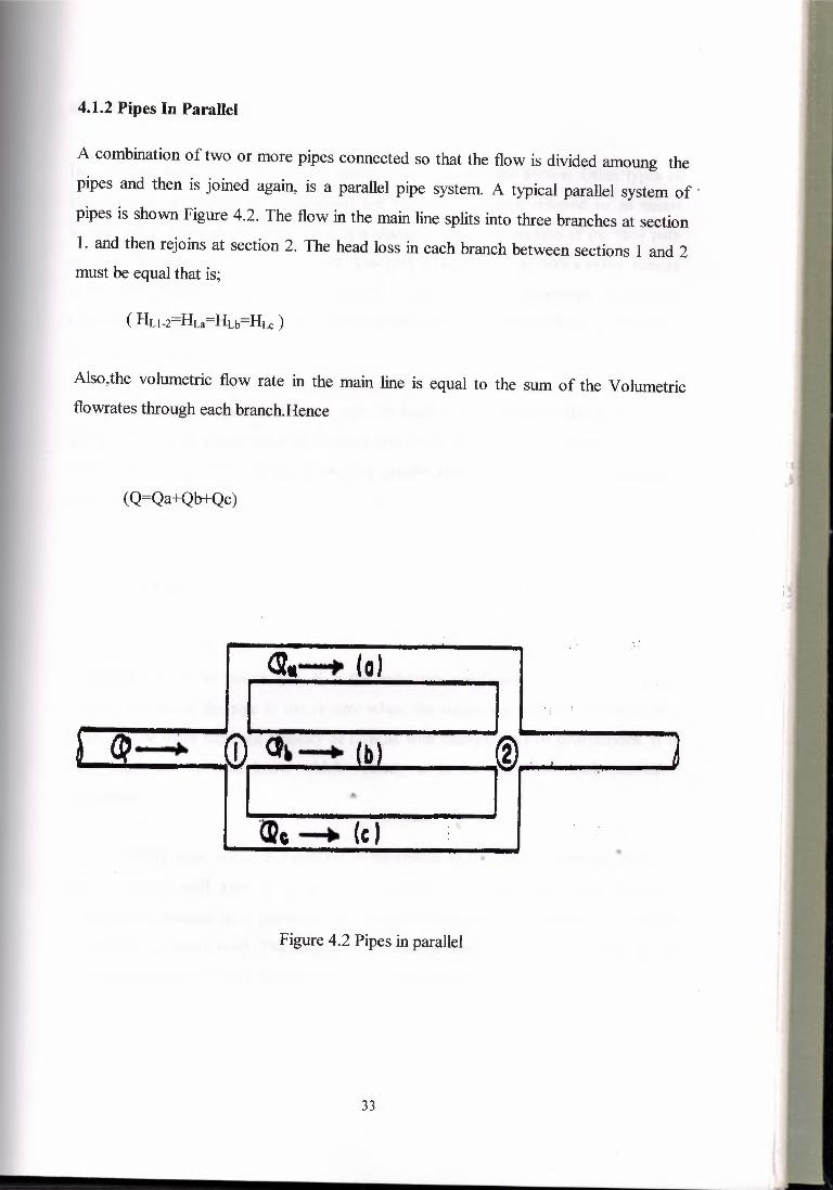
A combination of two or more pipes connected so that the flow is divided amoung the

pipes and then is joined again, is a parallel pipe system. A typical parallel system of ·

pipes is shown Figure 4.2. The flow in the main line splits into three branches at section

1. and then rejoins at section 2. The head loss in each branch between sections 1 and 2must be equal that is;

Also,the volumetric flow rate in the main line is equal to the sum of the Volumetricflowrates through each branch.Hence

(Q=Qa+Qb+Qc)

<2. ııı (a)

u} I••••• I ct~ • (b) ı®. I ••

~,-.+ (c) ~

••

Figure 4.2 Pipes in parallel

33

I.,

4.2 MINOR LOSSES

In most pipe flow system the primary energy loss is due to pipe friction. Other types of

losses are usually small by comparison and they are therefore referred to as minor

losses. Minor losses occur when there is a change in the cross section of the flow path

or in the direction of flow or where the flow path is obstructed, as with a valve. Energy

is lost under these conditions due to rather complex physical phenomena. Theoretical

prediction of the magnitude of these losses is also complex and therefore, experimental

data are normallyused.

Energy losses are proportional to the velocity head of the fluid as it flows around an

elbow, through an enlargement or constraction of the flow section or thr,ough a valve.

Experimental values for energy losses are usually reported in terms of a resistance

coefficient,Kas follows:

In Equation h1 is the minor loss, K is the resistance coefficient and u is the average

velocity of flow in the pipe in the vicinity where the minor loss occurs. In some cases,

there may be more than one velocity of flow,as with enlargements or contractions. It is

most important for you know which velocity is to be used with each resistance

coefficient.

If the velocity head u2 /2g in Equation is expressed in the units of meters,' then the

energy loss h1 will also be in meters or N.m/N of fluid flowing. The resistance

coefficient is unitless, as it represents a constant of proportionality between the energy

loss and the velocity head. The magnitude of the resistance coefficient depends on the

geometry of the device that causes the loss and sometimes on the velocity of flow.

34

4.2.1 Sudden Enlargement

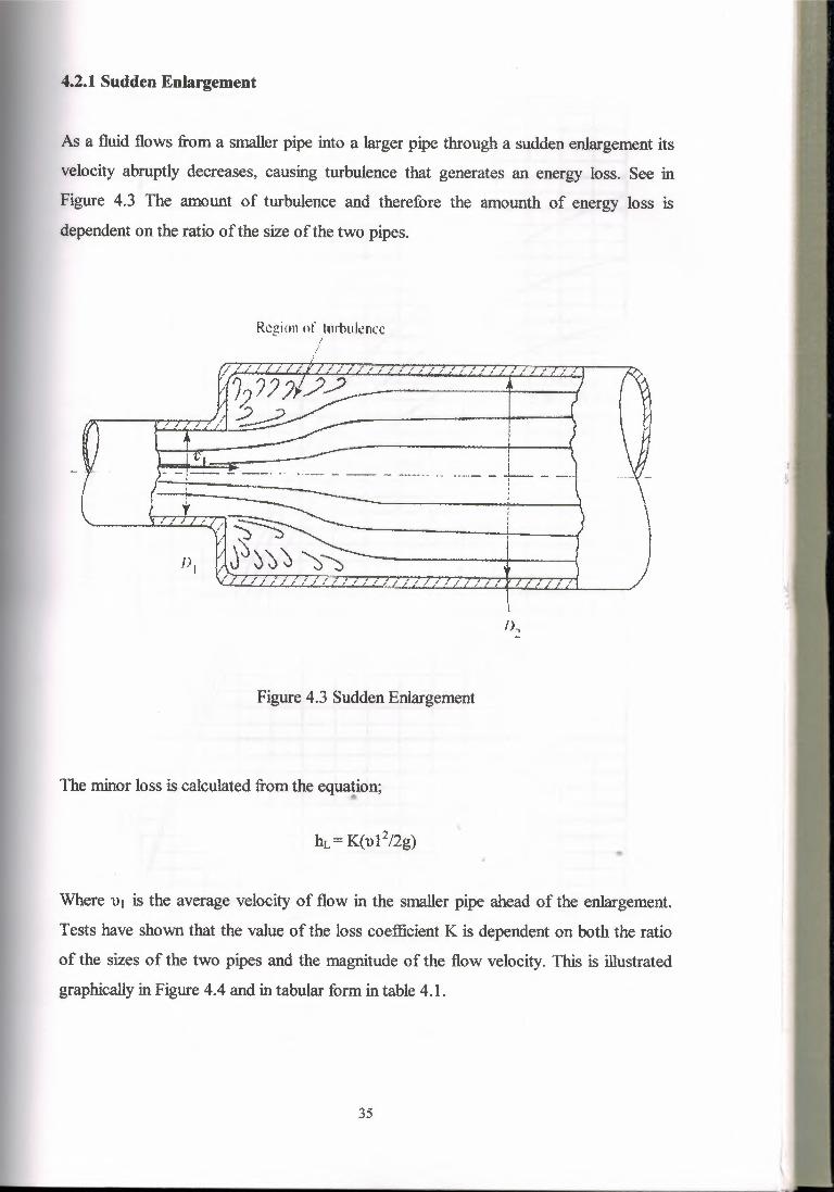
As a fluid flows from a smaller pipe into a larger pipe through a sudden enlargement its

velocity abruptly decreases, causing turbulence that generates an energy loss. See in

Figure 4.3 The amount of turbulence and therefore the amounth of energy loss is

dependent on the ratio of the size of the two pipes.

R~gimı of yırbuJçncc

II·-··-- - +- - -..-i

- - ı--- - ---· ..!

I),

Figure 4.3 Sudden Enlargement

The minor loss is calculated from the equation;

ıil

~.~

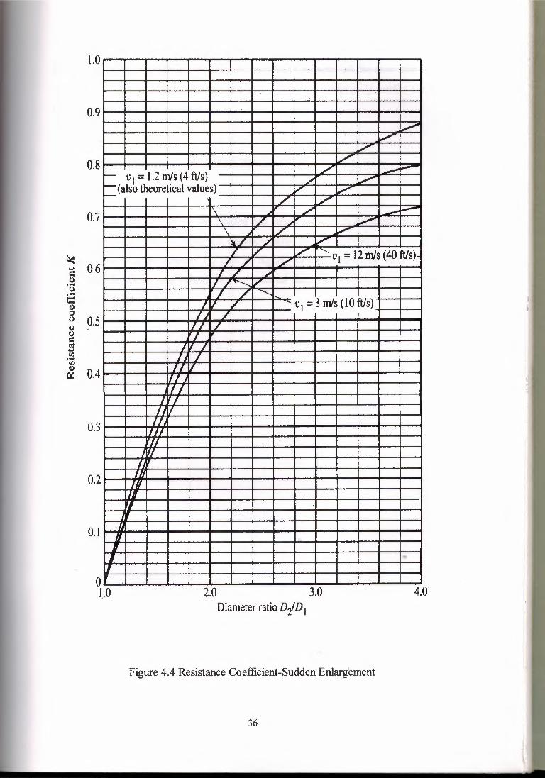
Where 1>1 is the average velocity of flow in the smaller pipe ahead of the enlargement.

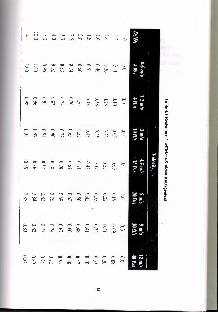
Tests have shown that the value of the loss coefficient K is dependent on both the ratio

of the sizes of the two pipes and the magnitude of the flow velocity. This is illustrated

graphicallyin Figure 4.4 and in tabular form in table 4.1.

35

~.•.. 0.6ı:II)...•C)!.:\j.,II)oo 0.5oı:;§r/J...•r/J

~ 0.4

I.O

0.9 _,~

././

/ ---- v1 = 1.2 mis (4 ft/s) _/ ----(also theoretical values) ,, _.,,- / ./

\ ~ ./ -- ---\ / ~' l...,,'"\ ~ . ./ .,,,,,.-

r:ı./ / .,,,,I/ v: l/ "v1 = 12 mis (40 ft/s).

J / /7 / j'

I J 1..-..._V I / / -......:...

I V l/ --- o1 == 3 mis (10 ft/s)I, /

II /I "I I /r, I

II II I,11

I I/JI

IIIll'II

. J "/,

'"'H '~~

j

/Ju ,

I -I

0.8

0.7

0.3

0.2

O.I

oLO 2.0 3.0 4.0

Diameter ratio Df D1

Figure 4.4 Resistance Coefficient-Sudden Enlargement

36

",ıy-

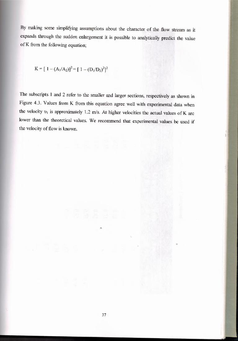
By making some simplifying assumptions about the character of the flow stream as it

expands through the sudden enlargement it is possible to analytically predict the value

ofK from the following equation;

K = [ 1 - (Aı/A2)]2 = [ 1 - (Dı/D2)2]2

The subscripts 1 and 2 refer to the smaller and larger sections, respectively as shown in

Figure 4.3. Values from K from this equation agree well with experimental data when

the velocity u1 is approximately 1 .2 mis. At higher velocities the actual values of K are

lower than the theoretical values. We recommend that experimental values be used ifthe velocity of flow is known.

:J,,,,

•

'J7

'? o r= o C, C C = = C = - ••• '""3-·~ ·...:; '-O ?C -....ı ---ı (.J'ı ~ '....,..J l'-1 C =oo o- ~ --·· X = o,. cc oc '!,..J) C, er ;-f'-•....~~ ı~

Ii...~...•.C C> -o ·O o - r= o C C s= ın• =.._, ..._, =-c: 00 '00 ?O ·--.J er. ......,, ~ u.) f',.) O• ,C) ~~ ~ ,o :.....;.,.) . ....,, I',,.) ,_;, ,...,, '..-) ....:::;, ~

~Q~s~... :)~=...•.I- <::;} -=· ~ ·O o = o = C o ·O r,ı- =OC· 00 00 ---1 -_a 0-, '.J1 ~ I_.....) l'.J 6 ·O Q.QC· C,.. 1.-..J 00 ·O !_,...} - v..ı -+'"- h.J 'C· Q.~=

t!!'j=-=.,(JQ~

C = c:, .::=;;, o o - o C - <=, =::-,-' - - ~~OC· 00 ce --.l er,. O' ~_ı·1 ..p.. '.,...) r~ o - =O' .ı. o 0--.. -s» l'.J o ı·,,.;ı '~ l.°'-J ·...c ...•.

••

-8 - ,...,, ..J;,.. ,:,....ı t--..ı t0-o ::..-. o = ı:....,-1; c:: 00 C,,-.; .p.. ('--.) o.-

o - - o ~ C· C <:;:::> '? ::-,o :O '-O '° ac ··--.] 0-- ~-.J't ~ f··.J -· --·O o O", r,J ı......ı ~ = - = C".

C C o C· C> ,o c:;, o - ,-. o C)- -oc oo -....:ı ---.jl O', O'- ::ı:,.. '.p.. l.;J 1'--1 - o-r..._,ı t-.J --..l ~ --...:a ·O Oô - t·..) - -c

o ...-.. C C o o o ·O C> o - o- -oe oo -..J -:ı O' ......,., ~ ~ t.H tv o oo t ...ı-ı t-...J v-ı. OC; ·---ı Cı 1'--> o ee

38

4.3 FRICTION LOSS IN TURBULENT FLOW

For turbulent flow of fluids in circular pipes it is most convenient to use Darcy's

equation to calculate the energy loss due to friction. We cannot determine the friction

factor f by a simple calculation as we did for laminar flow because turbulent flow does

not conform to regular predictable motions. It is rather chaotic and is constantly

varying. For these reasons we must rely on experimental data to determine thevalue off

Where

hL : Energy loss due to frictionless

L : Length of flow stream

D : Pipe diameter

v : Average velocityof flow

f : Friction factor

- ' }----,·- ! \I•. -- _i __ .,._,._

I 'I '

'.' o' ....!..~ .· . \

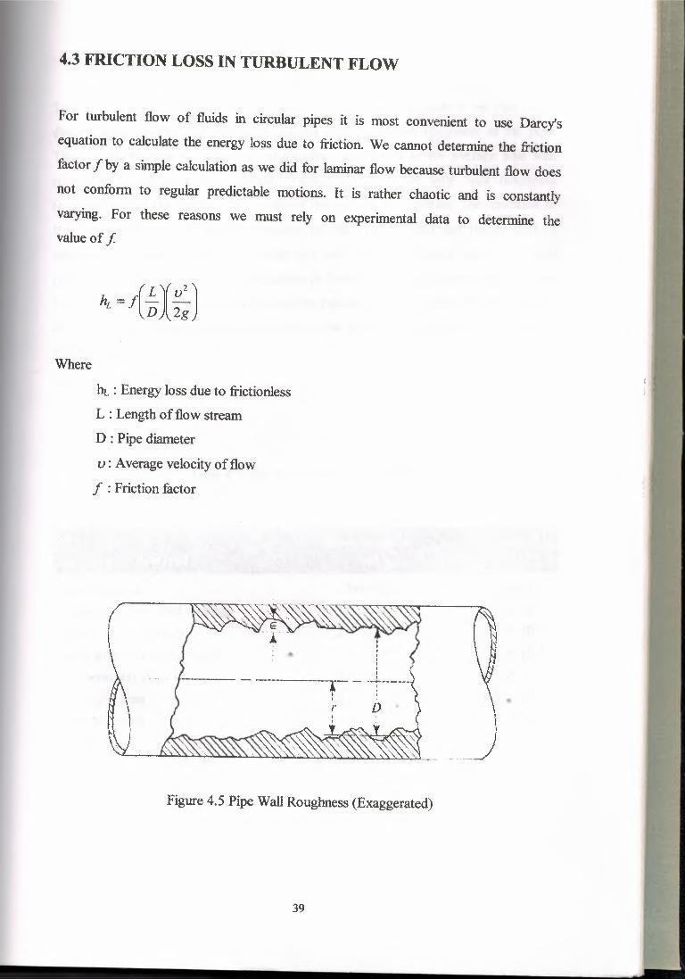
-----)Figure 4.5 Pipe Wall Roughness (Exaggerated)

39

Tests have shown that the dimensionless number f is dependent on two other

dimensionless numbers, the Reynolds number and the relative roughness of the pipe.

The relative roughness is the ratio of the pipe diameter D to the average pipe wall

roughness E (Greek letter epsilon). Figure 4.5 illustrates pipe wall roughness

(exaggerated) as the height of the peaks of the surface irregularities. The condition of

the pipe surface is very much depeı;ıdent on the pipe material and the method of

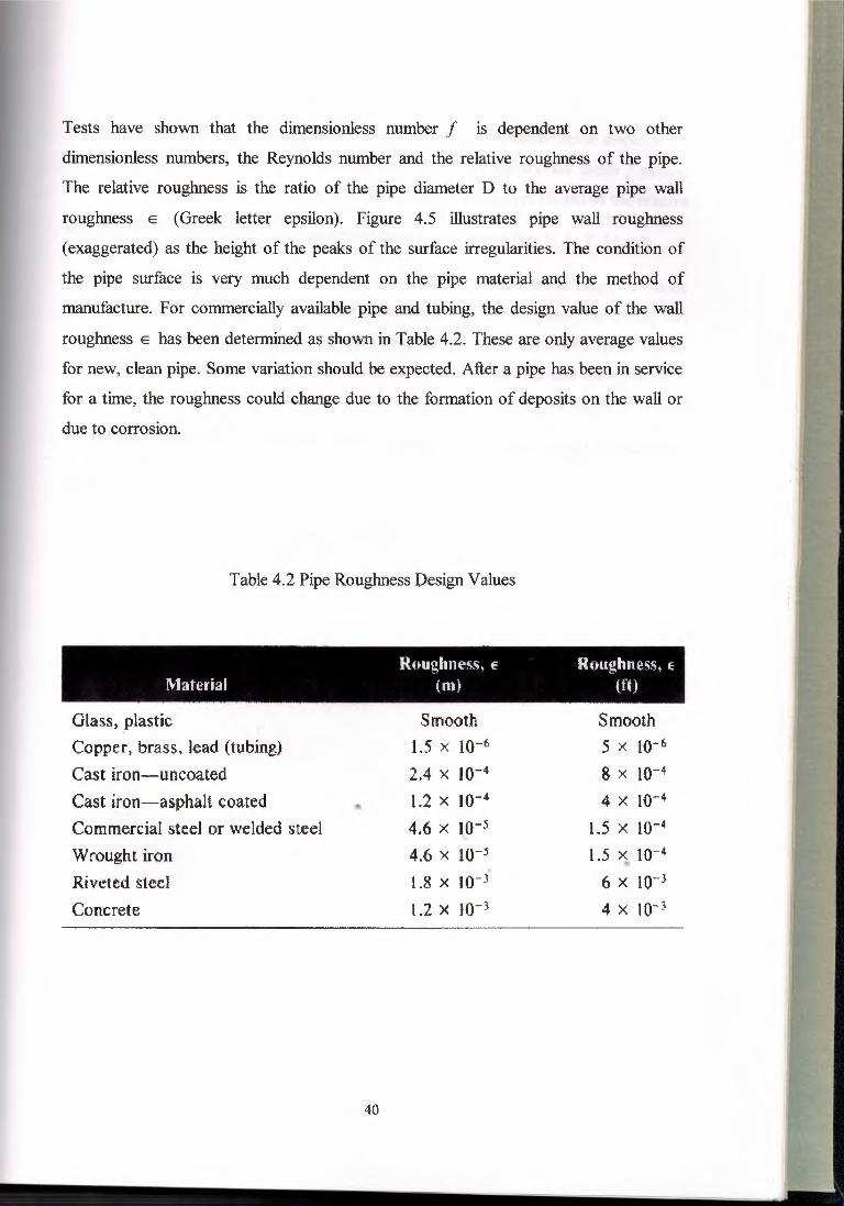
manufacture. For commercially available pipe and tubing, the design value of the wall

roughness E has been determined as shown in Table 4.2. These are only average values

for new, clean pipe. Some variation should be expected. After a pipe has been in service

for a time, the roughness could change due to the formation of deposits on the wall or

due to corrosion.

Table 4.2 Pipe Roughness Design Values

Roughness, e Roughness, E:

Material (m) (ft)

Glass, plastic Smooth SmoothCopper, brass, lead (tubing) 1.5 X ıo-6 5 X ıo-6

Cast iron-uncoated 2.4 X 10-4 8 X 10-4

Cast iron-asphalt coated .. l.2 X I0-4 4 X 10-4

Commercial steeJ or welded steel 4.6 X ıo-5 ı.s X }Q-4.,Wrought iron 4.6 X 10-5 1.5 ~ 10-4.Riveted steel 1.8 X ıo-3 6 X 10-J

Concrete l .2 X 10-3 4 X JO-:ı

40

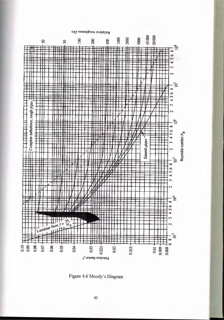
One of the most widely used method s for evaluating the friction factor employs the

Moody diagram shown in Figure 4.2. The diagram shows the friction factor f plotted

versus the Reynolds number Re, with a series of parametric curves related to the relative

roughness D . These curves were generated from experimental data by L. F. Moody.E

Both f and Re are plotted on logarithmic scales because of the broad range of values

encountered. At the left end of the chart, for Reynolds numbers less than 2000, the

straight line shows the relationshipf = 64/Re for laminar flow. For 2000 < NR < 4000,

no curves are drawn since this is the critical zone between laminar and turbulent flow

and it is not possible to predict the type of flow. Beyond Re = 4000, the familyof curves

for different values of D are plotted. Several important observations can be made fromE

these curves:

41

8•....• §•....•§ §o o--, N

~of 'ıoı:>eJuo~µd

ırı-oo

Figure 4.6 Moody's Diagram

42

QC)

o

.,,o-

....,o-

1. For a given Reynolds number of flow, as the relative roughness D is increased,E

the friction factorf decreases.

Reynolds number until the zone of complete turbulence is reached.

2. For a given relative roughness D , the friction factorf decreases with IncreasingE

3. Within the zone of complete turbulence, the Reynolds number has no effect onthe friction factor.

4. As the relative roughness D increases, the value of the Reynolds number atE

which the zone of complete turbulence begins also increases.

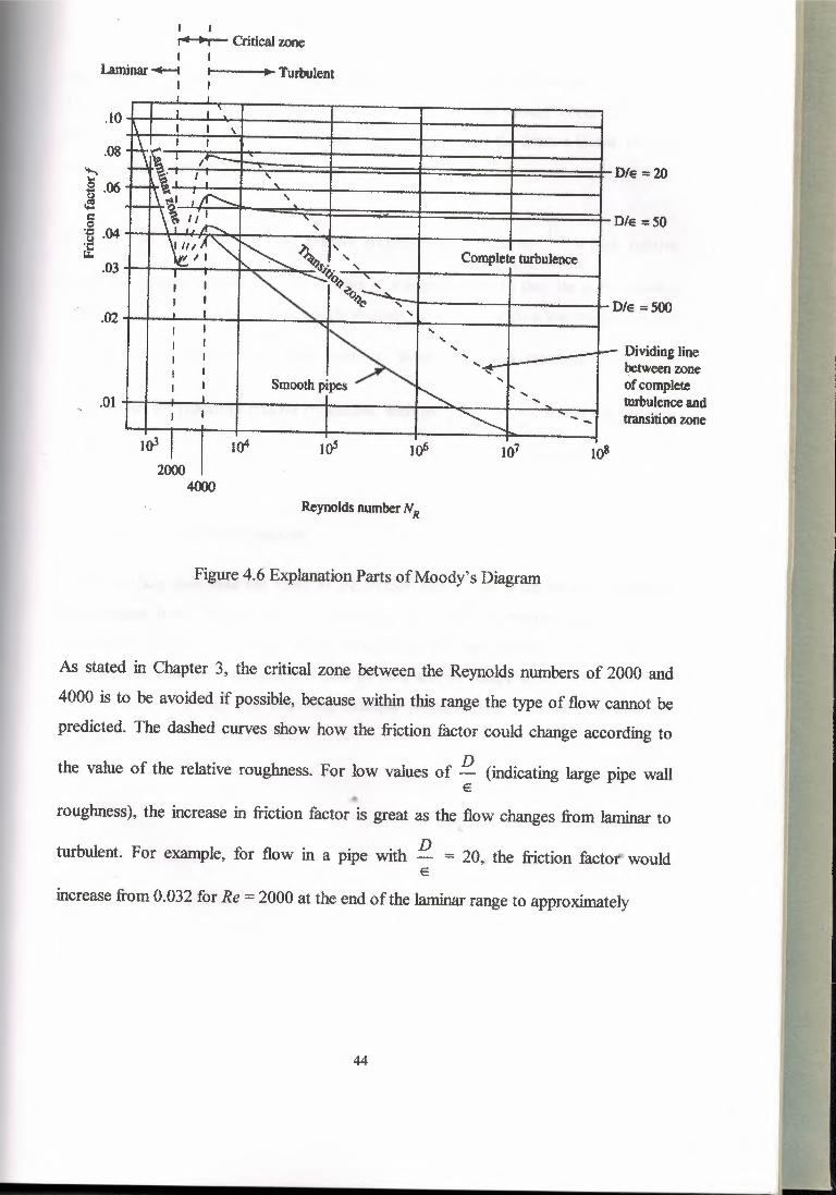
Figure 4.6 is a simplified sketch of Moody's diagram in which the various zones are

identified. The laminar zone at the left has already been discussed. At the right of the

dashed line downward across the diagram is the zone of complete turbulence. The

lowest possible friction factor for turbulent flow is indicated by the smooth pipes line.

Between the smooth pipes line and the line marking the start of the complete turbulence

zone is the transition zone. Here, the various D lines are curved, and care must beE

exercised to evaluate the friction factor properly. You can see, for example, that the

value of the friction factor for a relative roughness of 500 decreases from 0.0420 at Re=.4000 to 0.0240 at Re = 6.0 x Hl, where the zone of complete turbulence starts.

43

I II Ill •• I Critical zoneI I

Laminar .....-ı TurbulentI

.08';:>g .06 '!C 'C '·g .04 -t--t--'ı ..•...•~n- ..•..•:::ı------·c~ ı Complete turbulence J

fil I -

'°'-t-----+-----+- 0/e == 500.02;-""t------::----t-~~~~~~~~+-~~~-+~~~--ı

I ',' ' '~

'"

Die =20

I ...I

Die =SO

I II II II I

.oı I t I II I

ıoJ 1 I 10"2000

4000

....ı-- Dividing linebetween zone

',,tj of completeturbulence andtransition zone

1081 e>5 ıo6 ıo7

Reynolds number NR

Figure 4.6 Explanation Parts ofMoody's Diagram

As stated in Chapter 3, the critical zone between the Reynolds numbers of 2000 and

4000 is to be avoided if possible, because within this range the type of flow cannot be

predicted. The dashed curves show how the friction factor could change according to

the value of the relative roughness. For low values of D (indicating large pipe walle

roughness), the increase in friction factor is great as the flow changes from laminar to

turbulent. For example, for flow in a pipe with D = 20" the friction factor' wouldE

increase from 0.032 for Re= 2000 at the end of the laminarrange to approximately

44

45

0.077 at Re= 4000 at the beginning of the turbulent range, an increase of 240 percent.

Moreover, the value of the Reynolds number where this would occur cannot be

predicted. Because the energy loss is directly proportional to the friction factor, changesof such magnitude are significant.

It should be noted that because relative roughness is defined as D a high relativeE

roughness indicates a low value of E, that is, a smooth pipe. In fact, the curve labelled

smooth pipes is used for materials such as glass which, have such a low roughness that

D- would be an extremely large number. Some texts and references use otherE

• c. . 1· hn h EE r h is the niconventıons ıor reportıng re atıve roug ess, sue as - , - , or - , w ere r ıs t e pıpeD r E

radius.

4.3.1 Use of The Moddy Diagram

Is used to help determine the value of the friction factor Use of the Moody Diagram/

for turbulent flow. The value of the Reynolds number and the relative roughness must

be known. Therefore, the basic data required are the pipe inside diameter, the pipe

material, the flow velocity, and the kind of fluid and its temperature, from which the

viscosity can be found. The following example problems illustrate the procedure for

findirtg f

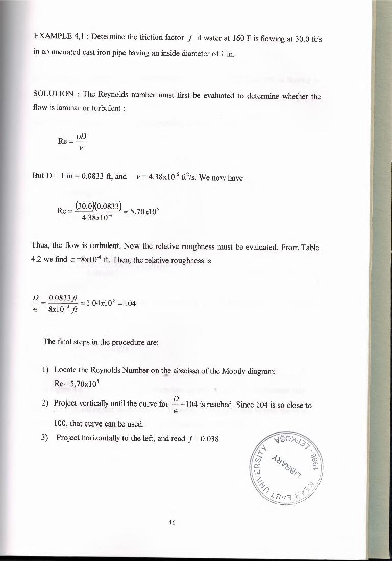
EXAMPLE 4,1 : Determine the friction factor f if water at 160 Fis flowingat 30.0 ft/s

in an uncuated cast iron pipe having an inside diameter of 1 in.

SOLUTION : The Reynolds number must first be evaluated to determine whether theflow is laminar or turbulent :

Re= vDV

But D = 1 in= 0.0833 ft, and v= 4.38x10-6ft2/s. We now have

(3o.oxo.0833) = 5.70xl05Re= 4.38xlo-6

Thus, the flow is turbulent. Now the relative roughness must be evaluated. From Table

4.2 we find E =8xl 04 ft. Then, the relative roughness is

D 0.0833ft = 1.04x102 = 104~ = 8xlff-4 ft

The final steps in the procedure are;

1) Locate the ReynoldsNumber on tqe abscissa of the Moody diagram:

R~= 5.70x105

2) Project verticallyuntil the curve for D =104 is reached. Since 104 is so close toE

100, that curve can be used.

3) Project horizontally to the left, and read/= 0.038

46

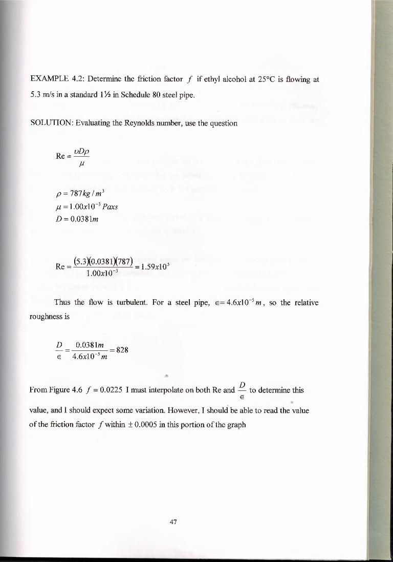
EXAMPLE 4.2: Determine the friction factor f if ethyl alcohol at 25°C is flowing at

5.3 mis in a standard I% in Schedule 80 steel pipe.

SOLUTION: Evaluating the Reynolds number, use the question

Re::;: vDpµ

p = 787kglm3

µ = 1.00xl0-3 Paxs

D = 0.0381m

(5.3X0.038IX787)= 1.59xl05

Re= 1.00xIO 3

Thus the flow is turbulent. For a steel pipe, E= 4.6xl0-5 m, so the relative

roughness is

D 0.038Im = 828- = 4.6xıo-s mE

Fro:\11 Figure 4.6 f = 0.0225 I must interpolate on both Re and D to determine thisE

value, and I should expect some variation. However, I should be able to read the value

of the friction factor f within ± 0.0005 in this portion of the graph

47

SUMMARY

In this chapter types of pipe line system which effect the energy losses and efficiency

are discussed, by using Moddy diagram which is used to determine friction factor are

considered.

When two pipes of different sizes or roughnesses are connected that fluid flows through

one pipe and then through the other, they are called connected in series. A combination

of two or more pipes and than is joined again is a parallel pipe system.

For turbulent flow of fluids incircular pipes it is most conveinent to use Darcy's

equation to calculate the energy loss due to friction.

Maddy's diagram in which the various zones are identified. It is used to help determine

the value of the friction for turbulent flow. The value of the Reynolds number and the

relative roughness must be known. Therefore the basic data required are the pipe inside

diameter, the pipe material, the flow velocity and the kind of fluid and its temperature,

from which the viscosity can be found.

••

48

CONCLUSION

Fluid mechanics is the science of the liquid and is based in three basic branches. They

are fluid statics, fluid kinematics, fluid dynamics. First chapter difference between

liquids and gases are examined as followed. Another important factor is viscosity,

which is a measure of the resistance the fluid has to shear. At the end of the chapter

Bernoulli's equation is determined and also described applications.

Second chapter laminar and turbulent flow are described. When the fluid flows in

smooth layers it is laminar flow, if much higher flow rates existed in the system it is

turbulent flow. According to the fluid are examined effect of viscosity and entrance

effects. Another categorizing flows are by exarninig the geometry of the flow field,

which are internal and external flows. Internal flow involved flow in an unbounded

region in the focus of attention is on the flow pattern a round a body immersed in the

fluids. In the third chapter is considered one and two dimensional flows and Reynolds

number. Reynolds number is one of several dimensionless numbers useful in the study

of fluid mechanics and heat transfer. Reynolds number is the ratio of the inertia force on

an element of fluid to the viscous force. If the Reynolds number is less than 2000 the

flow is laminar. Also, ıf the Reynols number is greater than 4000 the flow is turbulent.

The range ofReynols number is between 2000 and 4000, is called critical region.

Last chapter types of pipe line system which effect the energy losses and efficiencyare

discussed, by using Moddy diagram which is used to determine friction factor are

considered. When two pipes of different sizes or roughnesses are connected that :fluid

:flows through one pipe and then through the other, they are called connected in series...A combination of two or more pipes and than is joined again is a parallel pipe system.

For turbulent :flow of :fluids incircular pipes it is most conveinent to use Darcy's..•equation to calculate the energy loss due to friction. Moddy's diagram in which the

various zones are identified. It is used to help determine the value of the friction for

turbulent :flow. The value of the Reynolds number and the relative roughness must be

known. Therefore the basic data required are the pipe inside diameter, the pipe material,

the :flow velocity and the kind of :fluid and its temperature, from which the viscosity canbe found.

49

REFERENCES

1) IRVING H. SHOMES "Mechanics ofFluid" 2nd ed. Mc Graw-Hill International

Edditions, (Copyright 1995 USA)

2) ROBERT L . MOTT "Applied Fluid Mechanics" 4th ed. MacmillanPublishing

Company, (Copyright 1994 USA)

3) WILLIAM S . JANNA "Introduction to Fluid Mechanics" 2nded. PWS

PublishersEditions, (Copyright 1987 USA)

4) STREETER WYLIE BEDFORD "Fluid Mechanics" 9th ed. Mc Graw-Hill

International Editions, (Copyright 1998 USA)

"

50