Design of Highway Bridges forExtreme Events

NATIONALCOOPERATIVE HIGHWAYRESEARCH PROGRAMNCHRP

REPORT 489

TRANSPORTATION RESEARCH BOARD EXECUTIVE COMMITTEE 2003 (Membership as of March 2003)

OFFICERSChair: Genevieve Giuliano, Director and Professor, School of Policy, Planning, and Development, University of Southern California,

Los AngelesVice Chair: Michael S. Townes, Executive Director, Transportation District Commission of Hampton Roads, Hampton, VA Executive Director: Robert E. Skinner, Jr., Transportation Research Board

MEMBERSMICHAEL W. BEHRENS, Executive Director, Texas DOTJOSEPH H. BOARDMAN, Commissioner, New York State DOTSARAH C. CAMPBELL, President, TransManagement, Inc., Washington, DCE. DEAN CARLSON, Secretary of Transportation, Kansas DOTJOANNE F. CASEY, President, Intermodal Association of North AmericaJAMES C. CODELL III, Secretary, Kentucky Transportation CabinetJOHN L. CRAIG, Director, Nebraska Department of RoadsBERNARD S. GROSECLOSE, JR., President and CEO, South Carolina State Ports AuthoritySUSAN HANSON, Landry University Professor of Geography, Graduate School of Geography, Clark UniversityLESTER A. HOEL, L. A. Lacy Distinguished Professor, Department of Civil Engineering, University of VirginiaHENRY L. HUNGERBEELER, Director, Missouri DOTADIB K. KANAFANI, Cahill Professor and Chairman, Department of Civil and Environmental Engineering, University of California

at Berkeley RONALD F. KIRBY, Director of Transportation Planning, Metropolitan Washington Council of GovernmentsHERBERT S. LEVINSON, Principal, Herbert S. Levinson Transportation Consultant, New Haven, CTMICHAEL D. MEYER, Professor, School of Civil and Environmental Engineering, Georgia Institute of TechnologyJEFF P. MORALES, Director of Transportation, California DOTKAM MOVASSAGHI, Secretary of Transportation, Louisiana Department of Transportation and DevelopmentCAROL A. MURRAY, Commissioner, New Hampshire DOTDAVID PLAVIN, President, Airports Council International, Washington, DCJOHN REBENSDORF, Vice President, Network and Service Planning, Union Pacific Railroad Co., Omaha, NECATHERINE L. ROSS, Executive Director, Georgia Regional Transportation AgencyJOHN M. SAMUELS, Senior Vice President-Operations Planning & Support, Norfolk Southern Corporation, Norfolk, VAPAUL P. SKOUTELAS, CEO, Port Authority of Allegheny County, Pittsburgh, PAMARTIN WACHS, Director, Institute of Transportation Studies, University of California at BerkeleyMICHAEL W. WICKHAM, Chairman and CEO, Roadway Express, Inc., Akron, OH

MIKE ACOTT, President, National Asphalt Pavement Association (ex officio)MARION C. BLAKEY, Federal Aviation Administrator, U.S.DOT (ex officio)REBECCA M. BREWSTER, President and CEO, American Transportation Research Institute, Atlanta, GA (ex officio)THOMAS H. COLLINS (Adm., U.S. Coast Guard), Commandant, U.S. Coast Guard (ex officio)JENNIFER L. DORN, Federal Transit Administrator, U.S.DOT (ex officio)ELLEN G. ENGLEMAN, Research and Special Programs Administrator, U.S.DOT (ex officio)ROBERT B. FLOWERS (Lt. Gen., U.S. Army), Chief of Engineers and Commander, U.S. Army Corps of Engineers (ex officio)HAROLD K. FORSEN, Foreign Secretary, National Academy of Engineering (ex officio)EDWARD R. HAMBERGER, President and CEO, Association of American Railroads (ex officio)JOHN C. HORSLEY, Executive Director, American Association of State Highway and Transportation Officials (ex officio)MICHAEL P. JACKSON, Deputy Secretary of Transportation, U.S.DOT (ex officio)ROGER L. KING, Chief Applications Technologist, National Aeronautics and Space Administration (ex officio)ROBERT S. KIRK, Director, Office of Advanced Automotive Technologies, U.S. Department of Energy (ex officio)RICK KOWALEWSKI, Acting Director, Bureau of Transportation Statistics, U.S.DOT (ex officio)WILLIAM W. MILLAR, President, American Public Transportation Association (ex officio) MARY E. PETERS, Federal Highway Administrator, U.S.DOT (ex officio)SUZANNE RUDZINSKI, Director, Office of Transportation and Air Quality, U.S. Environmental Protection Agency (ex officio)JEFFREY W. RUNGE, National Highway Traffic Safety Administrator, U.S.DOT (ex officio)ALLAN RUTTER, Federal Railroad Administrator, U.S.DOT (ex officio)ANNETTE M. SANDBERG, Deputy Administrator, Federal Motor Carrier Safety Administration, U.S.DOT (ex officio)WILLIAM G. SCHUBERT, Maritime Administrator, U.S.DOT (ex officio)

NATIONAL COOPERATIVE HIGHWAY RESEARCH PROGRAM

Transportation Research Board Executive Committee Subcommittee for NCHRPGENEVIEVE GIULIANO, University of Southern California,

Los Angeles (Chair)E. DEAN CARLSON, Kansas DOTLESTER A. HOEL, University of VirginiaJOHN C. HORSLEY, American Association of State Highway and

Transportation Officials

MARY E. PETERS, Federal Highway Administration ROBERT E. SKINNER, JR., Transportation Research BoardMICHAEL S. TOWNES, Transportation District Commission

of Hampton Roads, Hampton, VA

T R A N S P O R T A T I O N R E S E A R C H B O A R DWASHINGTON, D.C.

2003www.TRB.org

NATIONAL COOPERATIVE HIGHWAY RESEARCH PROGRAM

NCHRP REPORT 489

Research Sponsored by the American Association of State Highway and Transportation Officials in Cooperation with the Federal Highway Administration

SUBJECT AREAS

Bridges, Other Structures, and Hydraulics and Hydrology

Design of Highway Bridges forExtreme Events

MICHEL GHOSN

FRED MOSES

AND

JIAN WANG

City College

City University of New York

New York, NY

NATIONAL COOPERATIVE HIGHWAY RESEARCH PROGRAM

Systematic, well-designed research provides the most effectiveapproach to the solution of many problems facing highwayadministrators and engineers. Often, highway problems are of localinterest and can best be studied by highway departmentsindividually or in cooperation with their state universities andothers. However, the accelerating growth of highway transportationdevelops increasingly complex problems of wide interest tohighway authorities. These problems are best studied through acoordinated program of cooperative research.

In recognition of these needs, the highway administrators of theAmerican Association of State Highway and TransportationOfficials initiated in 1962 an objective national highway researchprogram employing modern scientific techniques. This program issupported on a continuing basis by funds from participatingmember states of the Association and it receives the full cooperationand support of the Federal Highway Administration, United StatesDepartment of Transportation.

The Transportation Research Board of the National Academieswas requested by the Association to administer the researchprogram because of the Board’s recognized objectivity andunderstanding of modern research practices. The Board is uniquelysuited for this purpose as it maintains an extensive committeestructure from which authorities on any highway transportationsubject may be drawn; it possesses avenues of communications andcooperation with federal, state and local governmental agencies,universities, and industry; its relationship to the National ResearchCouncil is an insurance of objectivity; it maintains a full-timeresearch correlation staff of specialists in highway transportationmatters to bring the findings of research directly to those who are ina position to use them.

The program is developed on the basis of research needsidentified by chief administrators of the highway and transportationdepartments and by committees of AASHTO. Each year, specificareas of research needs to be included in the program are proposedto the National Research Council and the Board by the AmericanAssociation of State Highway and Transportation Officials.Research projects to fulfill these needs are defined by the Board, andqualified research agencies are selected from those that havesubmitted proposals. Administration and surveillance of researchcontracts are the responsibilities of the National Research Counciland the Transportation Research Board.

The needs for highway research are many, and the NationalCooperative Highway Research Program can make significantcontributions to the solution of highway transportation problems ofmutual concern to many responsible groups. The program,however, is intended to complement rather than to substitute for orduplicate other highway research programs.

Note: The Transportation Research Board of the National Academies, theNational Research Council, the Federal Highway Administration, the AmericanAssociation of State Highway and Transportation Officials, and the individualstates participating in the National Cooperative Highway Research Program donot endorse products or manufacturers. Trade or manufacturers’ names appearherein solely because they are considered essential to the object of this report.

Published reports of the

NATIONAL COOPERATIVE HIGHWAY RESEARCH PROGRAM

are available from:

Transportation Research BoardBusiness Office500 Fifth Street, NWWashington, DC 20001

and can be ordered through the Internet at:

http://www.national-academies.org/trb/bookstore

Printed in the United States of America

NCHRP REPORT 489

Project C12-48 FY’98

ISSN 0077-5614

ISBN 0-309-08750-3

Library of Congress Control Number 2003105418

© 2003 Transportation Research Board

Price $35.00

NOTICE

The project that is the subject of this report was a part of the National Cooperative

Highway Research Program conducted by the Transportation Research Board with the

approval of the Governing Board of the National Research Council. Such approval

reflects the Governing Board’s judgment that the program concerned is of national

importance and appropriate with respect to both the purposes and resources of the

National Research Council.

The members of the technical committee selected to monitor this project and to review

this report were chosen for recognized scholarly competence and with due

consideration for the balance of disciplines appropriate to the project. The opinions and

conclusions expressed or implied are those of the research agency that performed the

research, and, while they have been accepted as appropriate by the technical committee,

they are not necessarily those of the Transportation Research Board, the National

Research Council, the American Association of State Highway and Transportation

Officials, or the Federal Highway Administration, U.S. Department of Transportation.

Each report is reviewed and accepted for publication by the technical committee

according to procedures established and monitored by the Transportation Research

Board Executive Committee and the Governing Board of the National Research

Council.

The National Academy of Sciences is a private, nonprofit, self-perpetuating society of distinguished schol-ars engaged in scientific and engineering research, dedicated to the furtherance of science and technology and to their use for the general welfare. On the authority of the charter granted to it by the Congress in 1863, the Academy has a mandate that requires it to advise the federal government on scientific and techni-cal matters. Dr. Bruce M. Alberts is president of the National Academy of Sciences.

The National Academy of Engineering was established in 1964, under the charter of the National Acad-emy of Sciences, as a parallel organization of outstanding engineers. It is autonomous in its administration and in the selection of its members, sharing with the National Academy of Sciences the responsibility for advising the federal government. The National Academy of Engineering also sponsors engineering programs aimed at meeting national needs, encourages education and research, and recognizes the superior achieve-ments of engineers. Dr. William A. Wulf is president of the National Academy of Engineering.

The Institute of Medicine was established in 1970 by the National Academy of Sciences to secure the services of eminent members of appropriate professions in the examination of policy matters pertaining to the health of the public. The Institute acts under the responsibility given to the National Academy of Sciences by its congressional charter to be an adviser to the federal government and, on its own initiative, to identify issues of medical care, research, and education. Dr. Harvey V. Fineberg is president of the Institute of Medicine.

The National Research Council was organized by the National Academy of Sciences in 1916 to associate the broad community of science and technology with the Academy’s purposes of furthering knowledge and advising the federal government. Functioning in accordance with general policies determined by the Acad-emy, the Council has become the principal operating agency of both the National Academy of Sciences and the National Academy of Engineering in providing services to the government, the public, and the scientific and engineering communities. The Council is administered jointly by both the Academies and the Institute of Medicine. Dr. Bruce M. Alberts and Dr. William A. Wulf are chair and vice chair, respectively, of the National Research Council.

The Transportation Research Board is a division of the National Research Council, which serves the National Academy of Sciences and the National Academy of Engineering. The Board’s mission is to promote innovation and progress in transportation by stimulating and conducting research, facilitating the dissemination of information, and encouraging the implementation of research results. The Board’s varied activities annually engage more than 4,000 engineers, scientists, and other transportation researchers and practitioners from the public and private sectors and academia, all of whom contribute their expertise in the public interest. The program is supported by state transportation departments, federal agencies including the component administrations of the U.S. Department of Transportation, and other organizations and individuals interested in the development of transportation. www.TRB.org

www.national-academies.org

COOPERATIVE RESEARCH PROGRAMS STAFF FOR NCHRP REPORT 489

ROBERT J. REILLY, Director, Cooperative Research ProgramsCRAWFORD F. JENCKS, Manager, NCHRPDAVID B. BEAL, Senior Program OfficerEILEEN P. DELANEY, Managing EditorANDREA BRIERE, Associate EditorBETH HATCH, Assistant Editor

NCHRP PROJECT C12-48 PANELField of Design—Area of Bridges

THOMAS POST, CH2M Hill, Sacramento, CA (Chair) BARRY W. BOWERS, South Carolina DOTKAREN C. CHOU, Minnesota State University, Mankato, MN CHRISTOPHER DUMAS, FHWAROBERT G. EASTERLING, Cedar Crest, NM THEODORE V. GALAMBOS, University of Minnesota, Minneapolis, MN JOSE GOMEZ, Virginia DOTVIJAYAN NAIR, University of Michigan, Ann Arbor, MI ROBERT J. PERRY, Schenectady, NY PHIL YEN, FHWA Liaison RepresentativeSTEPHEN F. MAHER, TRB Liaison Representative

AUTHOR ACKNOWLEDGMENTSThis report was written by Professor Michel Ghosn of the City

College of the City University of New York/CUNY; Professor FredMoses from the University of Pittsburgh; and Mr. Jian Wang,Research Assistant at the City College and the Graduate Center ofCUNY. The authors would like to acknowledge the contributions ofseveral participants and individuals who have contributed in vari-ous ways to the work presented in this report.

Dr. Roy Imbsen, Dr. David Liu, and Dr. Toorak Zokaie fromImbsen & Associates, Inc., helped with the earthquake models, pro-vided bridge data, and assisted with project administration. Profes-sor Peggy Johnson of Penn State University developed the scourreliability model. Professor George Mylonakis from CUNY con-tributed valuable input on foundation and S.S.I. modeling. Mr. PeterBuckland and Mr. Darrel Gagnon from Buckland & Taylor assistedin the Maysville Bridge analysis and provided foundation analysismodels. Mr. Mark Hunter from Rowan, Williams, Davies, & Irwin,

Inc., performed the wind analysis of I-40 and Maysville bridges. Mr.Engin Aktas, Research Assistant at Pittsburgh, helped with thedevelopment of the live load model. Mr. Chuck Annis from Statisti-cal Engineering, Inc., assisted in the statistical analysis of scour data.

Dr. Emil Simiu from NIST contributed input on wind load mod-els. Dr. Arthur Frankel and E.V. Leyendecker from the U.S. Geo-logical Survey provided the earthquake hazard data. Ms. CharlotteCook and Ms. Debra Jackson from the U.S. Army Corps of Engineersprovided the Mississippi vessel data. Mr. Henry Bollman, FloridaDOT, contributed input on the vessel collision and scour models.

The authors are also especially grateful to the support and guid-ance provided by the project panel and the project director, Mr.David Beal. The project panel consisted of Mr. Thomas Post (Chair),Mr. Barry W. Bowers, Dr. Karen C. Chou, Mr. Christopher Dumas,Dr. Robert G. Easterling, Dr. Theodore V. Galambos, Dr. JoseGomez, Dr. Vijayan Nair, Dr. Robert J. Perry, and Dr. Phil Yen.

NCHRP Report 489: Design of Highway Bridges for Extreme Events contains thefindings of a study to develop a design procedure for application of extreme event loadsand extreme event loading combinations to highway bridges. The report describes theresearch effort leading to the recommended procedure and discusses the application ofreliability analysis to bridge design. The material in this report will be of immediateinterest to bridge engineers and bridge-design specification writers.

The magnitude and consequences of extreme events such as vessel collisions, scourcaused by flooding, winds, and earthquakes often govern the design of highwaybridges. If these events are considered to occur simultaneously, the resulting loadingcondition may dominate the design. This superpositioning of extreme load values fre-quently increases construction costs unnecessarily because a simultaneous occurrenceof two or more extreme events is unlikely. The reduced probability of simultaneousoccurrence for each load combination may be determined using statistical procedures.

The AASHTO LRFD Bridge Design Specifications developed under NCHRP Proj-ect 12-33 cover the basic design combinations with dead load and live load. Extremeload combinations were not considered in the load resistance factor design (LRFD) cal-ibration because of the lack of readily available data concerning the correlation ofextreme events. Nevertheless, a probability-based approach to bridge design forextreme events can be accomplished through incorporation of state-of-the-art reliabil-ity methodologies.

The objective of NCHRP Project 12-48 was to develop a design procedure for theapplication of extreme event loads and extreme event loading combinations to high-way bridges. This objective has been achieved with a recommended design procedureconsistent with the uniform reliability methodologies and philosophy included in theAASHTO LRFD Bridge Design Specifications. Four new extreme event load combina-tions are included to maintain a consistent level of safety against failure caused by scourcombined with live load, wind load, vessel collision, and earthquake, respectively.

This research was performed at the City College of the City University of NewYork, with the assistance of Dr. Fred Moses. The report fully documents the method-ology used to develop the extreme load combinations and the associated load factors.Recommended specification language is included in a published appendix. All appen-dixes to the report are included on CRP-CD-30.

FOREWORDBy David B. Beal

Staff OfficerTransportation Research

Board

1 SUMMARY

7 CHAPTER 1 Introduction1.1 Load Combinations in Current Codes, 71.2 Combination of Extreme Events for Highway Bridges, 91.3 Reliability Methods for Combination of Extreme Load Effects, 101.4 Reliability-Based Calibration of Load Factors, 131.5 Research Approach, 151.6 Report Outline, 16

17 CHAPTER 2 Reliability Models for Combinations of Extreme Events2.1 Loads and Return Periods in AASHTO LRFD, 172.2 Basic Concepts of Structural Reliability, 202.3 Resistance Models, 232.4 Load Models, 272.5 Risk Assessment Models for Load Combinations, 452.6 Chapter Conclusions, 49

50 CHAPTER 3 Calibration of Load Factors for Combinations of Extreme Events3.1 Description of Basic Bridge Configurations and Structural Properties, 503.2 Reliability Analysis for Extreme Events, 603.3 Reliability Analysis for Combinations of Extreme Events and

Calibration of Load Factors, 773.4 Summary and Recommendations, 96

100 CHAPTER 4 Conclusions and Future Research4.1 Conclusions, 1004.2 Future Research, 102

106 REFERENCES

108 GLOSSARY OF NOTATIONS

110 APPENDIXES Introduction, 110Appendix A: Recommended Modifications to AASHTO

LRFD Bridge Design Specifications, 111Appendix B: Reliability Model for Scour Analysis, 125Appendix C: Reliability Analysis of Three-Span Bridge Model, 128Appendix H: Seismic Risk Analysis of a Multispan Bridge, 152Appendix I: Analysis of Scour Data and Modified Reliability

Model for Scour, 162

CONTENTS

The current AASHTO load resistance factor design (LRFD) specifications weredeveloped using a reliability-based calibration that covered gravity loads consisting ofthe basic combination of permanent (or dead) load plus live load. The other load com-binations were obtained from previous generations of specifications and from the expe-rience of bridge engineers and, thus, may not be consistent with the reliability method-ology of the LRFD specifications. The objective of this study is to develop a designprocedure for the consideration of extreme events and the combination of their loadeffects in the AASHTO LRFD Bridge Design Specifications. Extreme events are definedas man-made or environmental hazards having a high potential for producing structuraldamage but are associated with a relatively low rate of occurrence. The extreme eventsconsidered in this study include live loads, earthquakes, wind loads, ship collisionforces, and scour.

According to the AASHTO LRFD, bridges should be designed for a 75-year returnperiod. The probability that a bridge will be subjected in its 75-year design life to anextreme event of a certain magnitude depends on the rate of occurrence of the eventand the probability distribution of the event’s intensity. Generally speaking, there islow probability that several extreme events will occur simultaneously at any point intime within a bridge’s design life. Even when simultaneous occurrences do occur, thechances that all the events are at their highest intensities are very small. To account forthese low probabilities, engineers have historically used the one-third stress-reductionrule when combining extreme environmental events, such as wind or earthquake loads,with gravity loads. This rule, which dates back to the early years of the 20th century,has been discredited; it is generally accepted that a more appropriate procedure shoulduse load combination factors derived from the theory of structural reliability.

The aim of structural reliability theory is to account for the uncertainties encounteredduring the safety evaluation of structural systems or during the calibration of load andresistance factors for structural design codes. The uncertainties considered include thoseassociated with predicting the load-carrying capacity of a structure, the intensities ofthe extreme events expected to be applied during the structure’s design life, the fre-quency of these loading events, and the prediction of the effects of these events onthe structure.

SUMMARY

DESIGN OF HIGHWAY BRIDGES FOR EXTREME EVENTS

To ensure the safety of highway bridges under the combined effects of extremeevents, this study develops load factors appropriate for inclusion in the AASHTO LRFDdesign-check equations. The reliability analysis of the effects of each threat taken indi-vidually is performed using methods developed in previous bridge code calibrationefforts (for the live loads and ship collisions) and during the development of other struc-tural codes (for wind loads and earthquake loads). Because the current AASHTO spec-ifications for scour are not based on reliability methods, a scour reliability model isdeveloped for the purposes of this study. Results of reliability analysis of typical bridgeconfigurations under the effect of individual threats are used to define target reliabilitylevels for the development of load factors applicable for designing bridges that may besusceptible to combinations of threats.

To achieve the objectives of the study, this project first reviews the basic reliabilitymethodology used during previous code calibration efforts. Basic bridge configurationsdesigned to satisfy the current AASHTO specifications are analyzed to find the implicitreliability index values for different limit states when the bridges are subjected to liveloads, wind loads, earthquakes, vessel collisions, or scour. The limit states consideredinclude column bending, shearing failure, axial failure of bridge columns, bearing fail-ure of column foundations, and overtipping of single-column bents. The reliabilityanalysis uses appropriate statistical data on load occurrences and load intensities for thepertinent extreme events that are assembled from the reliability literature and UnitedStates Geological Survey (USGS) websites. Statistical data on member and foundationcapacities and load analysis models commonly used in reliability-based code calibra-tion efforts are also used. Reliability indexes are calculated for the same bridges whensubjected to combinations of extreme events using the Ferry-Borges model. The resultsare subsequently used to calibrate load combination factors appropriate for implemen-tation in the LRFD equations.

The Ferry-Borges model assumes that each extreme event type produces a sequenceof independent load effects, each lasting for an equal duration of time. The service lifeof the structure is then divided into equal intervals of time. The probability that a loadoccurs in an arbitrary time interval can be calculated from the event’s occurrence rate.Simultaneously, the probability distribution of the intensity of the load given that theevent has occurred can be calculated from statistical information on load intensities.The probability that a second event would occur in the same time interval when the firstload event is on can also be calculated from the rate of occurrence of the second loadand the time durations of each load. After calculating the probability density for thesecond load given that it has occurred, the probability of the intensity of the combinedload effects can be calculated using a convolution integral. The load combination prob-lem consists of predicting the maximum value of the combined load effects that is likelyto occur in the lifetime of the bridge. Although the Ferry-Borges model gives a sim-plified representation of the actual loading phenomenon, this model is more accuratethan other load combination rules such as Turkstra’s rule because it takes into consid-eration the rate of occurrence of the loads and their time durations. The probability dis-tribution of the maximum value of the combined load effect is used along with statis-tical data on bridge member and system resistances to find the probability of failure andthe reliability index, β.

The load factors proposed in this study are calibrated such that bridges subjected toa combination of events provide reliability levels similar to those of bridges with thesame configurations but situated in sites where one threat is dominant. Thus, the pro-posed load factors are based on previous experiences with “safe bridge structures” andprovide balanced levels of safety for each load combination. The results of this studyindicate that different threats produce different reliability levels; therefore, the target

2

3

reliability indexes for the combination of events are selected in most cases to providethe same reliability level associated with the occurrence of the individual threat withthe highest reliability index. Thus, when dealing with the combination of live load pluswind load or live load plus scour, the reliability index associated with live loads is usedas target. When studying the reliability of bridges subjected to the combination of windloads and scour, the reliability index associated with wind loads alone is chosen for tar-get. Similarly, when studying the reliability of vessel collision with scour or vessel col-lision with wind load, the reliability index associated with vessel collisions is used fortarget. For combinations involving earthquake loads, it is the reliability index associ-ated with earthquakes alone that is used for target even if the reliability for earthquakesalone produces a lower reliability index. Combinations involving earthquakes aretreated differently than other combinations because of the large additional capacity andresulting construction costs that would be required to increase the reliability levels ofbridges subjected to earthquake risks.

The analysis considers structural safety as well as foundation safety. For multicolumnbents, system safety is compared with member safety. The results show that the systemproduces a reliability index about 0.25 higher than the reliability index of the individ-ual members for two-column bents formed by unconfined concrete columns. Hence,the system factors calibrated under NCHRP Project 12-47 are applicable for the casesin which linear elastic analysis is performed to check bridge member safety (seeNCHRP Report 458: Redundancy in Highway Bridge Substructures [Liu et al., 2001]).NCHRP Project 12-47 calibrated system factors for application on the left-hand side ofthe design equation to complement the member resistance factor. The cases for whichthe application of system factors is possible include the analysis of bridges subjectedto combinations exclusively involving live loads, wind loads, and ship collision forces.The analysis for combinations involving earthquakes is based on the plastic behaviorof bridge bents; thus, system safety is directly considered and no system factors needto be applied. Scour causes the complete loss of the load-carrying capacity of a column,and bridge bents subjected to scour depths exceeding the foundation depth will havelittle redundancy. Thus, such failures should be associated with system factors on theorder of 0.80 as recommended by NCHRP Project 12-47.

Results of the reliability analyses indicate that there are large discrepancies amongthe reliability levels implied in current design practices for the different extreme eventsunder consideration. Specifically, the following observations are made:

• The AASHTO LRFD was calibrated to satisfy a target member reliability indexequal to 3.5 for gravity loads. The calculations performed in this study confirm thatbridge column bents provide reliability index values close to the target 3.5 for thedifferent limit states considered. These limit states include column bending andaxial failure for one-column and multicolumn bents, as well as overtipping of one-column bents. Bearing failure of the soil may produce lower reliability levelsdepending on the foundation analysis model used.

• The system reliability index for bridge bents subjected to earthquakes is found tobe on the order of 2.9 for moment capacity or 2.4 for overtipping of single-columnbents founded on pile extensions (drilled shafts) that can be inspected. Lower reli-ability index values are observed for other subsystems depending on the responsemodification factors used during the design of their components. Unlike the analy-sis for other hazards, the earthquake analysis procedure accounts for system capac-ity rather than for member capacity because the earthquake analysis process accountsfor plastic redistribution of loads and failure is defined as a function of the ductil-ity capacity of the members. Although this is relatively low compared with the

member reliability index for gravity loads, the engineering community is gener-ally satisfied with the safety levels associated with current earthquake design pro-cedures, and increases in the currently observed safety levels would entail higheconomic costs. For this reason, the target reliability index for load combinationcases involving earthquakes is chosen to be the same reliability index calculatedfor designs satisfying the current design criteria when earthquakes alone areapplied. On the other hand, a future review of the response modification factorsused in earthquake design is recommended in order to produce more uniform reli-ability levels for all system types.

• The reliability index for designing bridge piers for scour in small rivers varies fromabout 0.45 to 1.8, depending on the size of the river and the depth and speed of thedischarge flow. These values are much lower than the 3.5 target for gravity loads andare also lower than the index values observed for earthquakes. In addition, failurescaused by scour may often lead to total collapse as compared with failures of mem-bers under gravity loads. Therefore, it is recommended to increase the reliabilityindex for scour by applying a scour safety factor equal to 2.0. The application ofthe recommended 2.0 safety factor means that if current HEC-18 scour design pro-cedures are followed, the final depth of the foundation should be 2.0 times the valuecalculated using the HEC-18 equation. Such a safety factor will increase the relia-bility index for scour from an average of about 1.0 for small rivers to a value slightlyhigher than 3.0, which will make the scour design safety levels compatible with thesafety levels for other threats. However, a review of the HEC-18 equations is rec-ommended in order to provide more uniform safety levels for all river categories.

• While bridge design methods for wind loads provide an average member reliabil-ity index close to 3.0, there are large differences among the reliability indexesobtained for different U.S. sites. For this reason, it is recommended that futureresearch in wind engineering develop new wind design maps that would providemore uniform safety levels for different regions of the United States.

• The AASHTO vessel collision model produces a reliability index of about 3.15 forshearing failures and on the order of 2.80 for bending failures. The presence of sys-tem redundancy caused by the additional bending moment resistance by the bents,abutments, or both that are not impacted would increase the reliability index forbending failures to more than 3.00, making the safety levels more in line with thosefor shearing failures.

The recommended load combination factors are summarized in Appendix A in a for-mat that is implementable in the AASHTO LRFD specifications. The results illustratethe following points:

• The current load factors for the combination of wind plus live loads lead to lowerreliability indexes than do those of either load taken separately. Hence, this studyhas recommended increasing the load factors for wind on structures and wind onlive loads from the current 0.40 to 1.20 in combination with a live load factor of1.0 (instead of the current live load factor of 1.35).

• The commonly used live load factor equal to 0.50 in combination with earthquakeeffects would lead to conservative results. This report has shown that a load fac-tor of 0.25 on live load effects when they are combined with earthquake effectswould still provide adequate safety levels for typical bridge configurations sub-jected to earthquake intensities similar to those observed on either the west or eastcoasts. These calculations are based on conservative assumptions on the recurrenceof live loads when earthquakes are actively vibrating the bridge system.

4

5

• For the combination of vessel collision forces and wind loads, a wind load factorequal to 0.30 is recommended in combination with a vessel collision factor of 1.0.The low wind load factor associated with vessel collisions compared with that rec-ommended for the combination of wind loads plus live loads partially reflects thelower rate of collisions in the 75-year design life of bridges as compared with thenumber of live load events.

• A scour factor equal to 1.80 is recommended for use in combination with a live loadfactor equal to 1.75. The lower scour load factor for the combination of scour andlive loads reflects the lower probability of having the maximum possible 75-yearlive load occur when the scour erosion is also at its maximum 75-year depth.

• A scour factor equal to 0.70 is recommended in combination with a wind load fac-tor equal to 1.40. The lower scour factor observed in combination with wind loadsas compared with the combination with live loads reflects the lower number ofwind storms expected in the 75-year design life of the structure.

• A scour factor equal to 0.60 is recommended in combination with vessel collisionforces. The lower scour factor observed in combination with collision forcesreflects the lower number of collisions expected in the 75-year bridge design life.

• A scour factor equal to 0.25 is recommended in combination with earthquakes.The lower scour factor with earthquakes reflects the fact that, as long as a totalwashout of the foundation does not occur, bridge columns subjected to scourexhibit lower flexibilities that will help reduce the inertial forces caused by earth-quakes. This reduction in inertial forces partially offsets the scour-induced reduc-tion in soil depth and the resulting soil-resisting capacity.

With regard to the extreme loads of interest to this study, the recommended revisionsto the AASHTO LRFD Bridge Design Specifications (1998) would address the loads byensuring that the factored member resistances are greater than the maximum loadeffects obtained from the following combinations (see following paragraphs for vari-able definition):

• Strength I Limit State: 1.25 DC + 1.75 LL• Strength III Limit State: 1.25 DC + 1.40 WS• Strength V Limit State: 1.25 DC + 1.00 LL + 1.20 WS + 1.20 WL• Extreme Event I: 1.25 DC + 0.25 LL + 1.00 EQ• Extreme Event II: 1.25 DC + 0.25 LL + 1.00 CV, or

1.25 DC + 0.30 WS + 1.00 CV• Extreme Event III: 1.25 DC; 2.00 SC, or

1.25 DC + 1.75 LL; 1.80 SC• Extreme Event IV: 1.25 DC + 1.40 WS; 0.70 SC• Extreme Event V: 1.25 DC + 1.00 CV; 0.60 SC• Extreme Event VI: 1.25 DC + 1.00 EQ; 0.25 SC

The presence of scour is represented by the variable SC. The semicolon indicates thatthe analysis for load effects should assume that a maximum scour depth equal to γSC SCexists when the other load events are applied where SC is the scour depth calcu-lated from the HEC-18 equations. When scour is possible, the bridge foundationshould always be checked to ensure that the foundation depth exceeds 2.00 SC. Forthe cases involving a dynamic analysis such as the analysis for earthquakes, it is crit-ical that the case of zero scour depth be checked because in many cases, the presenceof scour may reduce the applied inertial forces. The resistance factors depend on thelimit states being considered. When a linear elastic analysis of single and multicolumn

bents is used, the system factors developed under NCHRP Project 12-47 should alsobe applied.

In the equations given above, DC represents the dead load effect, LL is the live loadeffect, WS is the wind load effect on the structure, WL is the wind load acting on thelive load, EQ is the earthquake forces, CV is the vessel collision load, and SC repre-sents the design scour depth. The dead load factor of 1.25 would be changed to 0.9 ifthe dead load counteracts the effects of the other loads.

The recommended changes in the AASHTO LRFD consist of adding Extreme EventCases III through VI, which consider scour. In addition, Extreme Event II is modifiedto include a check of either live loads or wind loads with vessel collision forces. Ahigher wind load factor than live load factor is used to reflect the fact that the rate ofvessel collisions increases during the occurrence of windstorms.

6

7

CHAPTER 1

INTRODUCTION

This study is concerned with the safety of bridges sub-jected to the combination of four types of extreme load events:(1) earthquakes, (2) winds, (3) scour, and (4) ship collisions.In addition, these loads will combine with the effects of trucklive loads and the effects of dead loads. To ensure the safetyof highway bridges under the combined effects of extremeevents, this study develops load factors appropriate for inclu-sion in the AASHTO LRFD design-check equations. Struc-tural reliability methods are used during the load factor cal-ibration process in order to be consistent with the LRFDphilosophy and to account for the large uncertainties asso-ciated with the occurrence of such extreme events, estimat-ing their intensities, and analyzing their effects on bridgestructures.

Analytical models to study the probability of single eventsand multiple load occurrences are available in the reliabilityliterature and have been used to calibrate a variety of struc-tural design codes ranging from buildings, to offshore plat-forms, to nuclear power plants, to transmission towers, toships. This chapter describes the research approach followedduring the course of this study, provides an overview of howcurrent codes consider load combinations of extreme events,and describes how reliability analysis methods can be used tocalibrate load factors.

1.1 LOAD COMBINATIONS IN CURRENT CODES

Historically, engineers used the one-third stress-reductionrule when combining extreme environmental events, suchas wind or earthquake loads, with gravity loads. This rule,which dates to the early 20th century, has been discreditedand replaced by load combination factors derived from reli-ability analyses. The reliability-based effort on load combi-nations has eventually lead to the development of the Amer-ican National Standards Institute (ANSI) A58 Standard(ANSI A58 by Ellingwood et. al., 1980). The ANSI docu-ment set the stage for the adoption of similar load combina-tion factors in current generation of structural design codessuch as the Manual of Steel Construction (American Instituteof Steel Construction [AISC], 1994), also called the AISCManual; ACI 318-95 (American Concrete Institute [ACI],1995); AASHTO LRFD Bridge Design Specifications(AASHTO, 1998); and many other codes.

The total number of load combinations covered in AASHTOLRFD Bridge Design Specifications includes five combina-tions to study the safety of bridge members for strength limitstates, two load combinations for extreme load events, threeload combinations for service load conditions, and finally thefatigue loading. The loads in these combinations include theeffects of the permanent loads (which cover the weights ofthe structural components, attachments, and wearing surface)and earth pressure. The transient loads include those causedby the motion of vehicles and pedestrians; environmentaleffects such as temperature, shrinkage, and creep; water pres-sure; the effect of settlements and foundations; ice; collision;wind; and earthquakes.

With regard to the extreme loads of interest to this study,the current version of the AASHTO LRFD specifications(AASHTO, 1998) addresses them through the followingcombinations:

• Strength I Limit State: 1.25 DC + 1.75 LL• Strength III Limit State: 1.25 DC + 1.40 WS• Strength V Limit State: 1.25 DC + 1.35 LL

+ 0.4 WS + 0.4 WL (1.1)• Extreme Event I: 1.25 DC + 1.00 EQ• Extreme Event II: 1.25 DC + 0.50 LL

+ 1.00 CV

DC is the dead load, LL is the live load, WS is the wind loadon structure, WL is the wind load acting on the live load, EQis the earthquake load, and CV is the vessel collision load.The dead load factor of 1.25 would be changed to 0.9 if thedead load counteracts the effects of the other loads.

The safety check involving EQ is defined in the AASHTOspecifications as “Extreme Event I, Limit State.” It coversearthquakes in combination with the dead load and a fractionof live load to “be determined on a project-specific basis,”although the commentary recommends a load factor equal to0.5. “Extreme Event II” considers 50% of the design liveload in combination with either ice load, vessel collisionload, or truck collision load. Wind loads are considered in“Strength Limit III,” in which they do not combine with thelive load, and in “Strength Limit V,” in which they do com-bine with the live load. It should be noted that the design(nominal) live load for the strength limit states was based onthe maximum 75-year truck weight combination and as such

should also be considered an extreme event situation. In moststrength limit states, it is the live load factor that changesfrom 1.75 down to possibly 0.5 when the other extreme loadsare associated with a load factor of 1.0. The one exception isthe wind load: when used alone with the dead load, it is asso-ciated with a 1.4 load factor and a 0.4 factor when combinedwith the live load. The AASHTO LRFD specifications do notconsider the possibility of combining wind, earthquake, andvessel collision, nor do they account for the effect of scour-weakened foundations when studying the safety under anyof the transient loads. Also, as mentioned above, the LRFDcommentary suggests that 0.50 LL may be added to the casewhen the earthquake load is acting, although the specifica-tions state that “it should be determined on a project-specificbasis.” The nominal values for the loads correspond to dif-ferent return periods depending on the extreme event. Thereturn periods vary widely from 50 years for wind, to 75years for live load, to 2,500 years for earthquakes, while theship collision design is decided based upon an annual failurerate. Although not specifically addressed in the AASHTOLRFD specifications, the design for scour as currentlyapplied based on FHWA HEC-18 models uses a 100-yearreturn period as the basis for safety evaluation. It is noted thatfor most load events, the design nominal values and returnperiods are associated with implicit biases that would in effectproduce return periods different than those “specified.” Forexample, the HL-93 design live load is found to be smallerthan the 75-year maximum live load calculated from the datacollected by Nowak (1999) (see NCHRP Report 368: Cali-bration of LRFD Bridge Design Code) by about a factor ofabout 1.20. Similarly, the wind maps provided by ASCE 7-95and adopted by the AASHTO LRFD specifications give abiased “safe” envelope to the projected 50-year wind speeds.These issues are further discussed in Chapter 2.

The load factors and load combinations specified in thecurrent version of the AASHTO LRFD specifications followthe same trends set by other structural codes that were cali-brated using reliability-based methods. For example, AISC’sManual of Steel Construction bases its load combinations onthe provisions of ANSI A58. These provisions account forthe dead load, live load (roof live load is treated separately),wind load, snow load, earthquake load, ice load, and flood-ing. The primary load combinations are 1.2 dead load plus1.6 live load and 0.5 of snow or ice or rain load, another com-bination considers 1.2 dead load plus 1.6 snow or ice plus 0.5live or 0.8 wind load. The 1.2 dead load is also added to 1.5times the nominal earthquake load plus 0.5 live load or 0.2times the snow load.

ANSI A58 has eventually been replaced by the ASCE 7-95document (American Society of Civil Engineers [ASCE],1995). The latter gives a long list of load combinations, someof which have been modified from earlier versions. For exam-ple, the primary combination for seismic load includes 1.2times the dead load, 1.0 times the earthquake load, and 0.5times the live load plus 0.2 times the snow load. This com-

8

bination uses a seismic load factor of 1.0 based on the NationalEarthquake Hazards Reduction Program recommendations(NEHRP, 1997) rather than on the 1.5 initially proposed inthe ANSI code. The magnitudes of the earthquake forces arebased on ground accelerations with 10% probability of beingexceeded in 50 years. This is equivalent to a 475-year returnperiod. Recent work by NEHRP has supported increasing theearthquake return period up to 2,500 years, although the lat-est recommendation allows for a two-thirds reduction in theearthquake magnitudes for certain cases. The return periodfor the wind loads is set at 50 years.

The ACI Building Code’s primary load combination is 1.4dead load plus 1.7 live load. When wind is considered, thecode includes a 1.7 wind load factor but then reduces the totalload by 25%. Earth pressure is treated in the same manner asthe live load. When fluid pressure is included, it is associatedwith a load factor of 1.4 and then added to 1.4 dead load and1.7 live load. Loads due to settlement, creep, temperature,and shrinkage are associated with a load factor of 1.4 andwhen added to dead and live load, a 25% reduction in thetotal load is stipulated.

Other agencies that have implemented specifications forload combinations include the U.S. Nuclear Regulatory Com-mission (US-NRC) and the American Petroleum Institute(API). The US-NRC Standard Review Plan (US-NRC, 1989)for nuclear power plants uses load combinations similar tothose provided in ASCE 7-95. Extreme event loads are eachtreated separately with a load factor of 1.0. The only differ-ence between the US-NRC and the ASCE 7-95 provisionsare the higher return periods imposed on the extreme eventloads, particularly the seismic accelerations.

1.1.1 Summary

All of the codes listed above were developed using reliability-based calibrations of the load factors; yet, it isobserved that the types of loads that are considered simultane-ously and the corresponding load factors differ considerablyfrom code to code. Some of the differences in the load factorsmay be justified because of variations in the relative magni-tudes of the dead loads and the transient loads for the differenttypes of structures considered (e.g., dead load to live load ratio).Also, in addition to assigning the load factors, an importantcomponent of the specifications is the stipulation of themagnitude of the design loads or the return period for eachload. For example, if the design wind load corresponds to the50-year storm with a load factor of 1.4, it may produce asimilar safety level as the 75-year storm with a load factor of1.0. One should also account for the hidden biases and conser-vativeness built into the wind maps and other load data. Finally,one should note that the safety level is related to the ratio of theload factor to the resistance factor. For example, if the loadfactor were set at 1.40 with a resistance factor of 1.0, itwould produce a similar safety level as a load factor of1.25 when associated with a resistance factor of 0.90.

Despite the justifications for the differences mentionedabove, variations in the load factors may still lead to differ-ences in the respective safety levels implicit in each code.These differences are mainly due to the nature of the cur-rently used reliability-based calibration process, which uses anotional measure of risk rather than an actuarial value. In mostinstances, the code writers propose (1) load return periods and(2) resistance and load factors based on a “calibration” withpast experience to ensure that new designs provide the same“safety levels” as existing structures judged to be “acceptablysafe.” Because the historical evolution of the AASHTO, ACI,AISC, and the other codes may have followed different paths,it is not surprising to see that the calibration process producesdifferent load combinations and different load factors. In addi-tion, most codes use the reliability of individual members asthe basis for the calibration process. However, different typesof structures have different levels of reserve strength suchthat for highly redundant structures, the failure of one mem-ber will not necessarily lead to the collapse of the whole struc-ture. Therefore, in many cases, the actual reliability of thesystem is significantly higher than the implied target relia-bility used during the calibration process. Even within onesystem, the reliability levels of subsystems may differ—forexample, for bridges, the superstructure normally formed bymultiple girders in parallel would have higher system reservethan would the substructure, particularly when the substruc-ture is formed by single-column bents.

In particular, the AASHTO LRFD specifications weredeveloped using a reliability-based calibration that coveredonly dead and live loads (Strength I Limit State) using a targetreliability index equal to 3.5 against first member failure. Theother load combinations were specified based on AASHTO’sStandard Specifications for Highway Bridges (AASHTO,1996); on common practice in bridge engineering; or on theresults obtained from other codes. Consequently, the currentprovisions in the AASHTO LRFD for load combinations maynot be consistent with the provisions of the Strength I LimitState and may not produce consistent safety levels, as was theoriginal intent of the specification writers.

In theory, when looking at the possibility of load combi-nations, an infinite number of combinations are possible. Forexample, the maximum combined live load and earthquakeload effect might occur with the largest earthquake, or thesecond largest earthquake, and so forth, depending on thecontribution of the live load in each case to the total effect.The purpose of the calibration process is to provide a set ofdesign loads (or return periods) associated with appropriateload factors to provide an “acceptably safe” envelope to allthese possible combinations. The term “acceptably safe” isused because absolute safety is impossible to achieve. Also,there is a trade-off between safety and cost. The safer the struc-ture is designed to be, the more expensive it will be to build.Hence, code writers must determine how much implicit costthey are willing to invest to build structures with extremelyhigh levels of safety.

9

The next section will review available methods to studythe reliability of structures subjected to the combination ofload events. This information will be essential to determinehow and when extreme load events will combine and whatload factors will provide a safe envelope to the risk of bridgefailure due to individual load events and the combination ofevents.

1.2 COMBINATION OF EXTREME EVENTS FOR HIGHWAY BRIDGES

The extreme events of concern to this project are transientloads with relatively low rates of occurrences and uncertainintensity levels. Once an extreme event occurs, its time dura-tion is also a random variable with varying length, depend-ing on the nature of the event. For example, truck loadingevents are normally of very short duration (on the order of afraction of a second to 2 to 3 seconds) depending on the lengthof the bridge, the speed of traffic, and the number of truckscrossing the bridge simultaneously (platoons). Windstormshave varying ranges of time duration and may last for a fewhours. Most earthquakes last for 10 to 15 sec while ship colli-sions are instantaneous events. On the other hand, the effects ofscour may last for a few months for live bed scour and for theremainder of the life of a bridge pier for clear water conditions.The transient nature of these loads, their low rate of occurrence,and their varying duration times imply that the probability ofthe simultaneous occurrence of two events is generally small.The exceptions are when one of the loads occurs frequently(e.g., truckloads); when the two loads are correlated (ship col-lision and windstorm); or when one of the loads lasts for longtime periods (scour or, to a lesser extent, wind).

Even when two load types occur simultaneously, there islittle chance that the intensities of both events will be closeto their maximum lifetime values. For example, the chancesare very low that the trucks crossing a bridge are very heav-ily loaded at the time of the occurrence of a high-velocitywindstorm. On the other hand, because ship collisions aremore likely to occur during a windstorm, the effect of highwind velocities may well combine with high-impact loadsfrom ship collisions. Also, once a bridge’s pier foundationshave been weakened because of the occurrence of scour, thebridge would be exposed to high risks of failure because ofthe occurrence of any other extreme event. Of the extremeevents of interest to this study, only ship collision and windspeeds are correlated events. Although scour occurs becauseof floods that may follow heavy windstorms, the time lagbetween the occurrence of a flood after the storm would jus-tify assuming independence between wind and scour events.

For the purposes of this study and following current prac-tice, it will be conservatively assumed that the intensity of anyextreme event will remain constant at its peak value for thetime duration of the event. The time duration of each eventwill be assumed to be a pre-set deterministic constant value.The occurrence of extreme load events may be represented

as depicted in Figure 1.1, which shows how the intensitiesmay be modeled as constant in time once the event occursalthough the actual intensities generally vary with time.

Methods to study the combinations of the effects of extremeevents on structural systems have been developed based onthe theory of structural reliability. Specifically, three analyt-ical models for studying the reliability of structures under theeffect of combined loads have been used in practical appli-cations. These are (1) Turkstra’s rule; (2) the Ferry-Borges(or Ferry Borges–Castanheta) model; and (3) Wen’s load coin-cidence method. In addition, simulation techniques such asMonte Carlo simulations are applicable for any risk analysisstudy. These methods are intended to calculate the probabil-ity of failure of a structure subjected to several transient loadsand have been used to calibrate a variety of structural codesranging from bridges, to buildings, to offshore platforms, tonuclear power plants, to transmission towers, to ships. Thenext section describes the background and the applicabilityof these methods.

1.3 RELIABILITY METHODS FORCOMBINATION OF EXTREME LOADEFFECTS

Early structural design specifications represented the loadcombination problem in a blanket manner by simply decreas-ing the combined load effect of extreme events by 25% (e.g.,ACI) or by increasing the allowable stress by 33% (e.g.,AISC–allowable stress design [ASD]). These approaches donot account for the different levels of uncertainties associatedwith each of the loads considered, nor do they consider therespective rates of load occurrence and duration. For exam-ple, these methods decrease the dead load effect by the samepercentage as the transient load effects although the dead

10

load is normally better known (has a low level of uncertainty),is always present, and remains constant with time. The use ofdifferent load factors depending on the probability of simul-taneous occurrences of the loads is generally accepted as themost appropriate approach that must be adopted by codes indealing with the combination of loads.

An accurate calibration of the load factors for the combi-nation of extreme loads requires a thorough analysis of thefluctuation of loads and load effects during the service life ofthe structure. The fluctuations of the load effects in time canbe modeled as random processes (as illustrated in Figure 1.1)and the probability of failure of the structure can be analyzedby studying the probability that the process exceeds a thresh-old value corresponding to the limit state under considera-tion. Each loading event can be represented by its rate ofoccurrence in time, its time duration, and the intensity of theload. In addition, for loads that produce dynamic responses,the effects of the dynamic oscillations are needed. Severalmethods of various degrees of accuracy and simplicity areavailable to solve this problem. Three particular methodshave been used in the past by different code-writing groups.These are (1) Turkstra’s rule, (2) the Ferry Borges–Castanhetamodel, and (3) Wen’s load coincidence method (for exam-ples, see Thoft-Christensen and Baker, 1982; Turkstra andMadsen, 1980; or Wen, 1977 and 1981). These load combi-nation models can be included in traditional first order relia-bility method (FORM) programs. In addition, Monte Carlosimulations can be used either to verify the validity of themodels used or to directly perform the reliability analysis.Results of the reliability analysis will be used to (1) select thetarget reliability levels and (2) verify that the selected loadfactors would produce designs that uniformly satisfy the tar-get reliability levels. Below is a brief description of the threeanalytical methods. Chapter 2 will provide a more detailed

Assumed Intensity

Inte

nsity

of

load

eff e

ct

time

Assumed Intensity

Actual Intensity

Actual Intensity

Figure 1.1. Modeling the effect of transient loads.

description of the method used in this study. Chapter 3 andthe appendixes provide illustrations on the application of theselected method of analysis and the results obtained.

1.3.1 Turkstra’s Rule

Turkstra’s rule (Turkstra and Madsen, 1980) is a deter-ministic (non-random) procedure to formulate a load combi-nation format for the design of structures subjected to thecombined effects of several possible loading events. The ruleis an over-simplification derived from the more advancedFerry Borges–Castanheta model. Assuming two load typesonly (e.g., live load plus wind load), the intensity of the effectof Load 1 is labeled as x1 and for Load 2, the intensity isdefined as x2. Both x1 and x2 are random variables that varywith time. Turkstra’s rule may be summarized as follows:

• Design for the largest lifetime maximum value of Load1 plus the value of Load 2 that will occur when the max-imum value of Load 1 is on.

• Also design for the lifetime maximum of Load 2 plusthe value of Load 1 that will occur when Load 2 is on.

• Select the larger of these two designs.

In practical situations, the value of the load that is not at itsmaximum is taken at its mean (or expected) value. Turkstra’srule can thus be expressed as follows:

(1.2)

where

Xmax,T = the maximum value for the combined loadeffects in a period of time T,

max(x1) = the maximum of all possible x1 values,max(x2) = the maximum of all possible x2 values,

x1 = the mean value of x1, andx2 = the mean value of x2.

The rule can be extended for more than two loads followingthe same logic. Although simple to use, Turkstra’s rule isgenerally found to provide inconsistent results and is oftenunconservative (Melchers, 1999).

1.3.2 Ferry Borges–Castanheta Model for Load Combination

The Ferry Borges–Castanheta model is herein describedfor two load processes and illustrated in Figure 1.2 (Turkstraand Madsen, 1980; Thoft-Christensen and Baker, 1982). Themodel assumes that each load effect is formed by a sequenceof independent load events, each with an equal duration. Theservice life of the structure is then divided into equal inter-

Xx x

x xTmax, max[max( ) ][ max( )]

= ++

1 2

1 2

11

vals of time, each interval being equal to the time duration ofLoad 1, t1. The probability of Load 1 occurring in an arbitrarytime interval can be calculated from the occurrence rate ofthe load. Simultaneously, the probability distribution of theintensity of Load 1 given that the load has occurred can becalculated from statistical information on load intensities.The probability of Load 2 occurring in the same time inter-val as Load 1 is calculated from the rate of occurrence ofLoad 2 and the time duration of Loads 1 and 2. After calcu-lating the probability density for Load 2 given that it hasoccurred, the probability of the intensity of the combinedloads can be easily calculated.

The load combination problem consists of predicting themaximum value of the combined load effect X, namely Xmax,T,that is likely to occur in the lifetime of the bridge, T. In thelifetime of the bridge there will be n1 independent occurrencesof the combined load, X. The maximum value of the n1 pos-sible outcomes is represent by

(1.3)

The maximum value of x2 that is likely to occur within a timeperiod t1 (i.e., when Load 1 is on) is defined as x 2 max, t1. SinceLoad 2 occurs a total of n2 times within the time period t1,x2 max, t1 is represented by

(1.4)

Xmax,T can then be expressed as

(1.5)

or

(1.6)

The problem reduces then to finding the maximum of n2

occurrences of Load 2, adding the effect of this maximum tothe effect of Load 1, then taking the maximum of n1 occur-rences of the combined effect of x1 and the n2 maximum ofLoad 2. This approach assumes that x1 and x2 have constantintensities during the duration of one of their occurrences.Notice that x1 or x2 could possibly have magnitudes equal tozero. If the intensities of x1 and x2 are random variables withknown probability distribution functions, then the probabil-ity distribution functions of the maximum of several eventscan be calculated using Equation 1.7.

The cumulative distribution of a single load event, Y, canbe represented as FY (Y*). FY (Y*) gives the probability thatthe variable Y takes a value less than or equal to Y*. Mostload combination studies assume that the load intensities areindependent from one occurrence to the other. In this case,the cumulative distribution of the maximum of m events that

X x xTn n

max, max max .= + ( )[ ]1 2

1 2

X x xTn

tmax, max,max[ ]= +1

1 2 1

x xtn

2 1 22

max, max[ ]=

X XTn

max, max[ ]=1

occur in a time period T can be calculated from the probabil-ity distribution of one event by

(1.7)

where m is the number of times the load Y occurs in the timeperiod T.

Equation 1.7 is obtained by realizing that the probabilitythat the maximum value of m occurrences of load Y is lessthan or equal to Y* if the first occurrence is less than or equalto Y*, and the second occurrence is less than or equal to Y*,and the third occurrence is less than or equal to Y*, and soforth. This is repeated m times, which leads to the exponent,m, in the right-hand-side term of Equation 1.7.

This approach, which assumes independence between thedifferent load occurrences, has been widely used in many pre-vious efforts of calibration of load factors for combined loadeffects. Although the Ferry-Borges model is still a simplifiedrepresentation of the actual loading phenomenon, this modelis more accurate than Turkstra’s rule because it takes into con-sideration the rate of occurrence of the loads and their timeduration. The Ferry Borges–Castanheta model assumes that

F Y F YY m Ym

max , ( *) ( *)=

12

the loads are constant within each time interval and are inde-pendent. However, in many practical cases, even when theintensities of the extreme load events are independent, therandom effects of these loads on the structure are not inde-pendent. For example, although the wind velocities fromdifferent windstorms may be considered independent, themaximum moments produced in the piers of bridges as aresult of these winds will be functions of modeling variablessuch as pressure coefficients as well as other statistical uncer-tainties that are correlated or not independent from storm tostorm. In this case, Equation 1.7 has to be modified to accountfor the correlation between the intensities of all m possibleoccurrences. This can be achieved by using conditional prob-ability functions; that is, Equation 1.7 can be used with pre-setvalues of the modeling factor that are assumed to be constantand then by performing a convolution over these correlatedvariables.

1.3.3 Wen’s Load Coincidence Method

Wen’s load coincidence method (Wen, 1977, 1981) isanother method to calculate the probability of failure of a

Inte

nsity

of

load

effe

ct 1

T

T

T

t2 t2 t2 t2 t2 t2 t2 t2 t2 t2 t2 t2

t1 t1 t1

Load 1 + Load 2

Load 2 n2=t1/t2

Load 1 n1=T/t1

time

time

time

Inte

nsity

of

load

effe

ct 2

In

tens

ity o

f C

ombi

ned

load

effe

cts

Figure 1.2. Illustration of combination of two load effects according toFerry Borges–Castanheta model.

structure subjected to combined loads. The load coincidencemethod is more complicated than the two previously describedapproaches, but it can be used for both linear and nonlinearcombinations of processes, including possible dynamic fluc-tuations. The load coincidence method was found to givevery good estimates of the probability of failure when com-pared with results of simulations. Unlike the two previouslylisted methods, which assume independence between twodifferent load types, the load coincidence method accountsfor the rate of occurrence of each load event and the rate ofsimultaneous occurrences of a combination of two or morecorrelated loads.

The Wen load coincidence method can be represented bythe following equation (Wen, 1981):

(1.8)

where

P(E,T) = the probability of reaching limit state E (e.g.,probability of failure or the probability of exceed-ing a response level denoted by E) in a timeperiod T;

n = the total number of load types each designatedby the subscripts i and j;

λi = the rate of occurrence of load type i;pi = the probability of failure given the occurrence of

load type i only;λij = the rate of occurrence of load types i and j simul-

taneously; andpij = the probability of failure given the occurrence of

load types i and j simultaneously.

The process can be extended for three or more loads. Forexample, with the combination of two load types such as thecombination of wind load and live load, n would be 2 andload type i may represent the live load, and load type j mayrepresent the wind load. The rate of simultaneous occur-rences of live load and wind load, λ ij,, would be calculatedfrom the rate of occurrence of the wind, the rate of occur-rence of the live load, and the time duration of each of theloads. The probability of failure of the bridge given that awind and a live load occurred simultaneously is pij.

Wen’s method is valid when the load intensities are pulse-like functions of time that last for very short duration. Wen’smethod is an extension of the one-load approach that assumesthat failure events are independent and occur following aPoisson process. The loads are assumed to have low rates ofoccurrences, and failure events are statistically independent.Correlation between the arrival of two different load types isconsidered through the λ ij term, while correlation betweenload intensities is considered through the proper calculationof the pij term. As with the case of the Ferry-Borges model,Wen’s method does not account for the fact that there is cor-

P E T p p Ti i ij ijj i

n

i

n

i

n

( , ) exp≈ − − +

+= +−

−

=∑∑∑1

11

1

1

λ λ L

13

relation among the probability of failure of different eventsthat may exist because of the presence of common modelingvariables. Adjustments to consider this effect are more diffi-cult to incorporate because of the Poissonian assumptions.

This study uses the Ferry-Borges model because it providesa more intuitive approach to the load combination problemthan does the mathematical formulation of Wen’s load coin-cidence method. The Ferry-Borges model is directly imple-mentable in Level II reliability programs as demonstrated byTurkstra and Madsen (1980) and can be modified to accountfor the correlation from the modeling uncertainties using con-ditional probability distribution functions. Similarly, MonteCarlo simulations can be easily applied to use the Ferry-Borges model, including the consideration of correlation ofload effects from different time intervals.

1.4 RELIABILITY-BASED CALIBRATION OF LOAD FACTORS

The calibration process performed for the Strength I LimitState of the AASHTO LRFD (see Equation 1.1) followed tra-ditional methods available in the reliability literature. Thesemethods are similar to those used during the development ofAISC’s Manual of Steel Construction (1994), ACI’s Build-ing Code Requirements for Structural Concrete ACI 318-95(1995), and many other recently developed structural designand evaluation codes. The purpose of the theory of structuralreliability is to provide a rational method to account for sta-tistical uncertainties in estimating the capacity of structuralmembers, the effects of the applied loads on a structural sys-tem and the random nature of the applied loads. Since absolutesafety is impossible to achieve, the objective of a reliability-based calibration is to develop criteria for designing build-ings and bridges that provide acceptable levels of safety.

The theory of structural reliability is based on a mathe-matical formulation of the probability of failure. On the otherhand, the absence in the reliability formulation of many poten-tial risks such as human errors, major defects, deliberate over-loads, and so forth implies that the calculated values of riskare only notional measures rather than actuarial values. Inaddition, the calibration process often uses incomplete sta-tistical information on the loads and resistance of structuralsystems. This is due to the limited samples of data normallyavailable for structural applications and because each partic-ular structure will be subjected during its service life to aunique and evolving set of environmental and loading condi-tions, which are difficult to estimate a priori. As an example,for bridges subjected to vehicular loads, such unique condi-tions may include the effect of the environment and mainte-nance schedules on the degradation of the structural materi-als affecting the strength and the particular site-dependenttruck weights and traffic conditions that affect the maximumlive load. The truck weights and traffic conditions are relatedto the economic function of the roadway, present and futureweight limits imposed in the jurisdiction, the level of

enforcement of such limits, the truck traffic pattern, and thegeometric conditions including the grade of the highway atthe bridge site as well as seasonal variations related to eco-nomic activity and weather patterns. Such parameters areclearly very difficult to evaluate, indicating that the proba-bility of failure estimates obtained from traditional reliabil-ity analyses are only conditional on many of these parame-ters that are difficult to quantify even in a statistical sense.

Because the reliability-based calibration gives only anotional measure of risk, new codes are normally calibrated toprovide overall levels of safety similar to those of “satisfac-tory” existing structures. For example, during the developmentof bridge codes, the specification writers would assemble a setof typical member designs that, according to bridge engineer-ing experts, provide an acceptable level of safety. Then, usingavailable statistical data on member strengths and loads, ameasure of the reliability of these typical bridges is obtained.In general, the reliability index, β, is the most commonlyused measure of structural safety. The reliability index, β, isrelated to the probability of failure, Pf, as shown in the fol-lowing equation:

Pf = Φ(−β) (1.9)

where Φ is the cumulative standard normal distributionfunction.

During the calibration of a new design code, the averagereliability index from typical “safe” designs is used as the tar-get reliability value for the new code. That is, a set of loadand resistance factors as well as the nominal loads (or returnperiods for the design loads) are chosen for the new code suchthat bridge members designed with these factors will providereliability index values equal to the target value as closely aspossible.

Moses and Ghosn (1985) found that the load and resis-tance factors obtained following a calibration based on “safedesigns” are insensitive to errors in the statistical database aslong as the same statistical data and criteria are used to find thetarget reliability index and to calculate the load and resistancefactors for the new code. Thus, a change in the load and resis-tance statistical properties (e.g., in the coefficients of variation)would affect the computed β values. However, the change willalso affect the β values for all the bridges in the sample popu-lation of “typical safe designs” and, consequently, the averageβ (which is also the target β). Assuming that the performancehistory of these bridges is satisfactory, then the target relia-bility index would be changed to the new “average,” and thefinal calibrated load and resistance factors would remain rel-atively the same.

The calibration process described above does not containany preassigned numerical values for the target reliabilityindex. This approach, which has traditionally been used inthe calibration of LRFD criteria (e.g., AISC, AASHTO), hasled code writers to choose different target reliabilities for dif-

14

ferent types of structural elements or for different types ofloading conditions. For example, in the AISC LRFD, a tar-get β equal to 3.5 may have been chosen for the reliability ofbeams in bending under the effect of dead and live loads. Onthe other hand, a target β equal to 4.0 may be chosen for theconnections of steel frames under dead and live loads, and atarget β equal to 2.5 may be chosen for beams under earth-quake loads. Such differences in the target reliability indexclearly reflect the economic costs associated with the selectionof βs for different elements and for different load conditions,as well as different interpretations of modeling variables.

As mentioned earlier, the failure of one structural compo-nent will not necessarily lead to the collapse of the structuralsystem. Therefore, in recent years there has been increasedinterest in taking into consideration the safety of the systemwhile designing new bridges or evaluating the safety of exist-ing ones. The same approach followed during the calibrationof new codes to satisfy reliability criteria for individual struc-tural members can also be used for the development of codesthat take into consideration the system effects. For example,Ghosn and Moses (1998) and Liu et al. (2001) proposed a setof system factors that account for the system safety and redun-dancy of typical configurations of bridge superstructures andbridge substructures. These system factors were calibrated tosatisfy the same “system” reliability levels as those of exist-ing “satisfactory” designs.

However, whether using system reliability or member reli-ability indexes for criteria, the discrepancies between theobserved βs for different load types raise the following ques-tion: if the reliability index β for live load is 3.5 and for earth-quake loads β is 2.5, what should be the target when com-bining live loads and earthquake loads? On the other hand,the discrepancies in the target reliabilities can be justifiedusing a risk-benefit argument. For example, codes shouldtolerate a higher risk for the design of bridges (or structures)against a particular event if the costs associated with reduc-ing this risk are prohibitive. This risk-benefit argument canbe formalized using the expected cost of a bridge or anystructure defined as

CT = CI + CF Pf (1.10)

where

CT = the expected total cost,CI = the initial cost for building the structure,CF = the cost of failure, andPf = the probability of failure.

The initial cost of a structure increases as the safety level isincreased. On the other hand, the probability of failuredecreases as the safety level increases. Thus, to provide anoptimum balance between risk and benefit, the target relia-bility index that should be used is the one that minimizes theexpected total cost, CT.

Although conceptually valid, the use of Equation 1.10 in anexplicit form has not been common in practice because of thedifficulties associated with estimating the cost of failure, CF.Instead, code writers have resorted to using different targetreliabilities for different types of members and loads based oncalibration with previous acceptable designs. A risk-benefitapproach is possible if the implicit costs of a structural fail-ure can be extracted based on current designs. Aktas, Moses,and Ghosn (2001) have demonstrated the possibility of usingthe risk-benefit analysis described in Equation 1.10; how-ever, more work is still needed in evaluating the relationshipbetween CI and CF before the actual implementation of thisapproach during the development of design codes.

Because more research is needed before the implementationof Equation 1.10 becomes possible, this report will use a tra-ditional method of calibrating the load factors to provide a tar-get reliability index that will be extracted based on satisfyingthe same safety levels of existing “satisfactory designs.” Forexample, because the reliability index obtained for bridges thatsatisfy current scour design procedures is relatively smallcompared with that obtained for bridges designed to satisfythe wind load requirements, the target reliability level thatwill be used for the combination of scour and wind will bechosen to be equal to the reliability level for bridges sub-jected to wind alone. This will ensure that bridges subjected tocombinations of wind loads and scour will have safety levelsas high as those that may be subjected to high winds. A simi-lar approach will be used when combining scour with otherextreme load events. For the load combinations involvingearthquakes, the reliability index obtained from earthquakesalone will be used for target. This is because the engineeringcommunity has determined that current earthquake design pro-cedures provide sufficient levels of safety in view of the enor-mous costs that would be implied with any increases in the cur-rent design procedures. By using the logic described in thisparagraph, a risk-benefit analysis is implicitly used in a rela-tively subjective manner.

1.5 RESEARCH APPROACH

The objective of this study is to develop design proceduresfor the application of extreme load events and the combinationof their load effects in AASHTO LRFD Bridge Design Speci-fications. The load events considered in this study will includelive loads, seismic loads, wind loads, ship collision loads, andscour. The design procedures will consist of a set of load fac-tors calibrated using reliability-based methods that are consis-tent with the reliability methodology of the AASHTO LRFDspecifications. The purpose of the AASHTO specifications isto provide procedures to proportion bridge members suchthat they will provide sufficient levels of safety in their ser-vice lives for any possible load type or combination of loads.This means that the bridges are expected to satisfy an accept-

15

able level of reliability that strikes a balance between safetyand cost.

To achieve the objectives of the study, this project will firstreview the basic reliability methodology used during previ-ous code calibration efforts. Models to study the reliability ofbridges subjected to the effects of each load taken individu-ally will be adopted from previous bridge code calibrationefforts (for the live loads and ship collisions) and from mod-els developed during the calibration of structural codes forbuildings (for wind loads and earthquake loads). Becauseexisting specifications for scour are not based on reliabilitymethods, a scour reliability model will be developed for thepurposes of this study.

Basic bridge configurations designed to satisfy the currentAASHTO specifications will be analyzed to find the implicitreliability index values for bridge design lives of 75 years andfor different limit states when these bridges are subjected tolive loads, wind loads, earthquakes, vessel collisions, or scour.The limit states that will be considered include column bend-ing, shearing failure, and axial failure of bridge columns, bear-ing failure of column foundations, and overtipping of single-column bents.

The reliability calculations will be based on assumed prob-ability distributions for the random variables describing theeffects of extreme load events on bridge structures. Theseassumed distributions will be based, where possible, on avail-able statistical data pertaining to these random variables. Tostudy the probability of load combinations, data on the rateof occurrence of each load event, the rate of occurrence ofsimultaneous load events, the magnitude of each load event,and the time duration of each load event will be required.This information will be assembled from the available relia-bility literature, as will be described in the next chapter. Also,available statistical data on the capacity of the bridge systemsto resist the applied loads will be needed. This information isavailable from reports describing the calibration efforts ofthe AASHTO LRFD specifications and other available infor-mation on the behavior of structures and foundation systems(e.g., Nowak, 1999; Poulos and Davis, 1980).

In addition to studying the reliability of the typical bridgeconfigurations under the effects of individual extreme events,the reliability analysis will be performed for these same bridgeconfigurations when they are subjected to the combined effectsof the extreme events under consideration. Reliability methodsfor combining the effects of several loads have been developedby researchers in the field of reliability, as described in Sec-tion 1.3. As explained earlier, the Ferry-Borges model forload combination will be used because it provides a simpleand reasonable model that is easy to implement. Modifica-tions on the classical Ferry-Borges model will be made toaccount for statistical and modeling uncertainties of time-dependent and time-independent random variables.

The reliability analysis will be performed for a numberof bridge configurations and for different modes of failure.

Because the extreme load events being considered are mostlyhorizontal loads that primarily affect the substructure ofbridges, the analysis will be performed for typical bridgebents subjected to lateral loading in the transverse direction.Emphasis will be placed on failure of the columns in bend-ing and of the foundation system subjected to lateral loads,although other failure modes such as shearing failures or axialcompression of column or foundation will be considereddepending on the applied load (e.g., shearing failures areimportant modes for barge collisions and axial compressionis important for the failure of multicolumn bents). Whenapplicable, such as in the case of bending of multicolumnbents, system effects will be taken into consideration.

The results of the reliability analyses will subsequently beused to calibrate load factors and load combination factorsthat will provide bridge designs with adequate levels ofsafety when subjected to extreme load events. To minimizethe changes to the current AASHTO specifications, the loadfactors will be applicable to the effects of the nominal loadscorresponding to the same return periods as those currentlyin use. The load factors will be calibrated such that bridgessubjected to a combination of events provide reliability lev-els similar to those of bridges with the same configurationsbut situated in sites where one threat is dominant. Thus, theproposed load factors will be based on previous experienceswith “safe bridge structures” and will provide balanced lev-els of safety for each load combination. As mentioned above,the target reliability indexes for the combination of eventswill be selected in most cases to provide the same reliabilitylevel associated with the occurrence of the individual threatwith the highest reliability index. Lower reliability index tar-get values may be justified in the cases (such as earthquakeloads) when increased reliability levels would result in unac-ceptable economic costs. The analysis will consider struc-tural safety as well as foundation safety and system safetywill be compared with member safety. The goal is to recom-mend a rational and consistent set of load factors that can beused during the routine design of highway bridges. Theseload factors will be presented in a specifications format thatcan be implemented in future versions of the AASHTO LRFDspecifications.

16

1.6 REPORT OUTLINE

This report is divided into four chapters and nine appen-dixes. Chapter 1 gave a review of the problem statement andan overview of the proposed research approach. Chapter 2describes the reliability models used in this study for the dif-ferent load applications and combinations of loads. Chapter 3provides the results of the reliability analysis of typical bridgeconfigurations subjected to the extreme events of interestand combinations of these events. Chapter 3 also provides theresults of the calibration process and determines the load fac-tors for the combinations of extreme events. Chapter 4 givesthe conclusion of this study and outlines future research needs.

Appendix A summarizes the results of this study in anAASHTO specifications format that provides the load factorsfor the combination of extreme events. The format is suitablefor implementation in future versions of AASHTO LRFDBridge Design Specifications. Appendix B details the relia-bility model for the analysis of scour as developed by Profes-sor Peggy Johnson for the purposes of this study. The relia-bility models used for the other extreme events were extractedfrom the literature and are similar to those used by otherresearchers during the calibration of various structural designcodes. Appendix C provides details of the reliability calcula-tions for a three-span bridge used as the basis for the calibra-tion. Appendix D describes the model used for the analysis ofa long-span arch bridge subjected to scour and earthquakes.Appendix E describes the analysis of a long-span bridge overthe Ohio River in Maysville for vessel collisions. AppendixF describes the earthquake analysis of the Maysville Bridge.Appendix G describes the wind analysis model for both theInterstate 40 and the Maysville Bridges. Appendix H describesthe reliability analysis model used for a multispan bridge sub-jected to earthquakes. Appendix I performs a statistical analy-sis of available scour data and proposes an alternative modelfor the reliability analysis of bridge piers under scour. Theexamples solved in the appendixes serve to provide detailsabout the models used in the body of the report and also to illus-trate how big projects can be specifically addressed in detail.

Appendixes A, B, C, H, and I are published herein. Allappendixes (Appendixes A through I) are contained on CRP-CD-30, which is included with this report.

17

CHAPTER 2

RELIABILITY MODELS FOR COMBINATIONS OF EXTREME EVENTS

This chapter describes the models used to perform the reli-ability analysis of bridges subjected to extreme load eventsand their combinations. The chapter is divided into six sec-tions. Section 2.1 presents the design nominal loads as spec-ified in the current AASHTO LRFD and reviews the currentcode’s methods for combining the effects of the extreme loadevents of interest to this study. Section 2.2 gives a brief reviewof the concepts of structural reliability theory and its appli-cation for calibration of structural design codes. Section 2.3describes the resistance models used for member and systemcapacity. Section 2.4 describes the reliability models for thepertinent individual loads. Section 2.5 describes the risk analy-sis model used for the combination of loads. Section 2.6 con-cludes the chapter.

2.1 LOADS AND RETURN PERIODS INAASHTO LRFD

The specification of load combinations in structural designcodes includes the required nominal (i.e., design) loads orreturn periods as well as their corresponding load factors.Figure 2.1 shows the table of load factors given in the currentAASHTO LRFD (Table 3.4.1). Nominal loads are usuallyassociated with some long-term historical event that definesthe loading. For example, the bridge design specificationsrequire the design for the 50-year wind, the 2,500-year earth-quake, the 75-year maximum live load, and the 100-year floodfor scour. The load factors used are normally equal to or greaterthan 1.0 when each load is analyzed individually. When theload factor is greater than 1.0, it means that the true returnperiod for the design event is greater than the specified nom-inal return period. This section reviews the current AASHTOnominal design loads and return periods for the loads of inter-est to this study.

2.1.1 Dead Load

The LRFD code uses a set of dead load factors that reflectthe differences in the levels of uncertainties associated withestimating the weight of cast-in-place elements (particularlywearing surfaces) to those of pre-cast elements. Followingcommon practice, the nominal (design) dead load is the bestestimate obtained from design plans for new bridges or frominspection of existing bridges.

2.1.2 Live Load

Nowak (1999) calibrated the nominal HL-93 design truckloading model to match a projected expected 75-year maxi-mum live load effect for all span ranges. The 75-year load pro-jection was obtained based on truck weight data collected inthe province of Ontario assuming a heavy volume (about 5,000trucks per day) of truck traffic. The HL-93 load model wasdeveloped to represent the effects of live loads on short- tomedium-span bridges for two-lane traffic. Multipresence fac-tors are used to account for the differences between the HL-93truck load effect and the expected maximum 75-year load forbridges with one lane or three or more lanes. Although theHL-93 load effects are slightly lower than the calculated max-imum 75-year load effects, it is noted that the Ontario dataused to calibrate the HL-93 load model contains a large levelof conservativeness because it is biased toward the heavilyloaded trucks. Similarly, the number of side-by-side eventsused to account for multiple-occurrence probabilities is alsohighly conservative. Moses (2001) gives a more completediscussion of these factors.

The HL-93 loading consists of a truck with similar con-figuration and axle weights as the HS-20 truck used in theAASHTO standard specifications (AASHTO, 1996). The truckhas axle weights of 35 kN, 145 kN, and 145 kN (8, 32, and32 Kips) along with axle spacing of 4.3 m (14 ft) and 4.3 to9.0 m (14 to 30 ft). In addition, the HL-93 model stipulatesthat a lane load of 9.3 N/mm (0.64 kip/ft) should be used. Forcontinuous bridges, two trucks are used (one in each span)along with the lane load. However, a reduction factor equalto 0.90 is included for multispan bridges. The dynamic fac-tor of 1.33 is applied to the truck load alone excluding theeffect of the lane load.

2.1.3 Earthquake Load

The design earthquake intensities specified in the currentAASHTO LRFD are based on a 475-year return period foressential bridges and 2,500-year return period for criticalbridges. Maps giving the design peak ground accelerationsfor different regions of the United States are provided byAASHTO (Figure 3.10.2; AASHTO, 1998) based on the workof NEHRP (NEHRP, 1997). The specified load factor is 1.0.The basis of the design is the inelastic response of bridges

due to earthquakes. The inelastic behavior and the ductilitycapacity of bridge members are reflected through the use ofthe response modification factor R. Thus, material nonlin-earity and system effects are indirectly taken into considera-tion. Also, the effect of the soil condition on the response isaccounted for by using different correction factors for differ-ent types of soil. The earthquake design spectrum is given interms of the natural frequencies of the bridge and is based onbest estimates of the weight and the bridge elastic stiffness.

NCHRP Project 12-49 has proposed a comprehensive set ofLRFD design specifications for the seismic design of bridges(see NCHRP Report 472: Comprehensive Specification forthe Seismic Design of Bridges [Applied Technology CouncilATC and the Multidisciplinary Center for Earthquake Engi-neering Research MCEER, 2002]). The proposed specifi-cations use the NEHRP 2,500-year return period earthquakehazard maps along with the response spectra proposed byNEHRP but remove a two-thirds reduction factor that was

18

associated with the NEHRP spectral accelerations. The two-thirds factor had been included by NEHRP to essentiallyreduce the 2,500-year spectrum to an equivalent 500-yearspectrum for the U.S. west-coast region.

2.1.4 Wind Load

The AASHTO LRFD wind load provisions are based on theassumption that no live loads will be present on the bridgewhen wind velocities exceed 90 km/h (56 mph). Accordingto the AASHTO LRFD commentaries, this assumption isbased on “practical experience.” The basic wind speed used is160 km/h (100 mph) although the option of using other valuesis permitted. Wind speeds may be taken from the ASCE7-95 provisions to reflect regional and geographical effects.The ASCE 7-95 maps have a return period of 50 years. Thestipulated AASHTO LRFD wind load factor of 1.4 indicates

LOAD

COMBINATION

LIMIT STATE

DC

DD

DW

EH

EV

ES

LL

IM

CE

BR

PL

LS

WA WS WL FR TU

CR

SH

TG SE EQ IC CT CV

Strength I γP 1.75 1.00 – – 1.00 0.50/

1.20

γTG γSE – – – –

Strength II γ P 1.35 1.00 – – 1.00 0.50/

1.20

γ TG γSE – – – –

Strength III γ P – 1.00 1.40 – 1.00 0.50/

1.20

γ TG γSE – – – –

Strength IV

EH, EV, ES, DW,

DC ONLY

γ P

1.5

– 1.00 – – 1.00 0.50/

1.20

– – – – – –

Strength V γ P 1.35 1.00 0.40 0.40 1.00 0.50/

1.20

γTG γ SE – – – –

Extreme Event I γP γ EQ 1.00 – – 1.00 – – – 1.00 – – –

Extreme Event II γP 0.50 1.00 – – 1.00 – – – – 1.00 1.00 1.00

Service I 1.00 1.00 1.00 0.30 0.30 1.00 1.00/

1.20

γ TG γ SE – – – –

Service II 1.00 1.30 1.00 – – 1.00 1.00/

1.20

– – – – – –

Service III 1.00 0.80 1.00 – – 1.00 1.00/

1.20

γ TG γ SE – – – –

Fatigue— LL, IM

and CE only

– 0.75 – – – – – – – – – – –

Figure 2.1. AASHTO LRFD load combination and load factor table (see Appendix A for definitionof table symbols).

that the effective return period is higher than 50 years. A com-parison between the ASCE 7-95 wind maps and the dataprovided by Simiu et al. (1979) and Ellingwood et al. (1980)reveal that the maps provide a conservative upper limit enve-lope to the actual measured maximum 50-year winds.

The AASHTO LRFD contains methods to perform thewind analysis based on boundary layer theory combined withempirical observations. For wind on live loads, the AASHTOLRFD uses a distributed force of 1.46 N/mm (0.1 kip/ft)at1800 mm (6 ft) above the roadway applied to the tributaryareas that “produce load effects of the same kind.” The 1.46N/mm corresponds to the 90 km/h (56 mph) wind speed thatis the limiting speed at which live load would be present onthe structure.

2.1.5 Vessel Collision

The AASHTO LRFD requirements for vessel collisionare based on the probability of bridge collapse using factorsrelated to the site, the barge size, and the geometry of thewaterway. According to AASHTO LRFD, the acceptableannual frequency of collapse is 0.0001 for critical bridgesand 0.001 for other bridges. AASHTO LRFD stipulates thatthe probability of collapse should be calculated based on thenumber of vessels, the probability of vessel aberrancy, thegeometric probability of collision given an aberrant vessel,and the probability of bridge collapse given a collision. TheAASHTO LRFD provides an empirical equation to obtainthe probability of bridge collapse given that a collision hasoccurred. Conservative assumptions are implicitly includedin many of the empirical equations used in the safety checkprocess (e.g., estimation of barge impact force), in effectfurther reducing the probability of collapse. The load factorspecified is set at 1.0.

2.1.6 Scour

The AASHTO LRFD specifications require that scour atbridge foundations be designed for the 100-year flood stormsurge tide or for the overtopping flood of lesser recurrenceinterval. The corresponding 100-year design scour depth atbridge foundations is estimated following the procedure rec-ommended by FHWA using the manual known as “HEC-18”(Hydraulic Engineering Circular No. 18: Evaluating Scourat Bridges [Richardson and Davis, 1995]). The foundationshould then be designed while taking into consideration thedesign scour depth. This is achieved by, for example, placingthe footings below the scour depth, ensuring that the lengthsof piles and pile shafts extend beyond the scour depth, andverifying that the remaining soil depth after scour providessufficient resistance against sliding failures and overturning.

The HEC-18 manual recognizes that the total scour at ahighway crossing is composed of three components: (1) long-term aggradation and degradation, (2) contraction scour, and

19

(3) local scour. Aggradation and degradation are long-termelevation changes in the streambed of the river or waterwaycaused by erosion and deposition of material. Contractionscour is due to the removal of material from the bed and thebanks of a channel often caused by the bridge embankmentsencroaching onto the main channel. Local scour involves theremoval of material from around bridge piers and abutments.It is caused by an acceleration of flow around the bridgefoundation that accompanies a rise in water levels that maybe due to floods and other events. Both local scour and con-traction scour can be either clear water or live bed. Live-bedconditions occur when there is a transport of bed material inthe approach reach. Clear-water conditions occur when thereis no bed material transport. Live-bed local scour is cyclic innature because it allows the scour hole that develops duringthe rising stage of the water flow to refill during the fallingstage. Clear-water scour is permanent because it does notallow for a refill of the hole. The focus of this report is onlocal live-bed scour around bridge piers that, because of itscyclical nature, is the most unpredictable type of scour.

Summary

Each loading type considered in the AASHTO LRFD pro-visions is represented by a nominal load intensity (i.e., a codespecified live load or a geographically varying load for agiven return period) and a corresponding load factor. It isnoticed that the design return periods differ considerably foreach type of load event (e.g., 2,500-year for earthquakes, 75-year for live load, 50-year for wind, 100-year for scour, and1-year for vessel collisions). The reasons for the differencesin the design return periods are traditional use, providingconsistency with other codes, and providing assurances tothe public about the safety of bridges. One should note thatthese return periods are only nominal because by adjustingthe load factors, one could produce a common “effectivereturn period.” In addition, several of the “event intensitymaps” provided as part of the specifications are based onbiased envelopes of the actual measured data, and the degreeof conservatism in each load analysis model varies from loadtype to load type. Therefore, actual failure rates may be sig-nificantly different than those implied by the nominal returnperiods. One major aim of structural reliability methods is toquantify these degrees of conservatism by obtaining morerealistic and objective assessments of the safety levels impliedin code-specified design procedures for each load type.

The calibration of the AASHTO LRFD specifications forthe Strength I Limit State was undertaken using uniform reli-ability criteria. The code was calibrated based on the reliabil-ity of individual girders of multigirder bridges for the combi-nation of dead and live loads. The specifications for the otherextreme events of interest to this study were based on the workperformed for other structural codes. In particular, AASHTOLRFD relies on the provisions and guidelines provided by

NEHRP for earthquakes, ASCE 7-95 for wind, AASHTO’sGuide Specification and Commentary for Vessel CollisionDesign of Highway Bridges for vessel collisions (AASHTO1991), and HEC-18 by FHWA for scour. In order to performthe reliability analysis and calibrate the load factors for com-binations of extreme load events, statistical information onthe rate of occurrence, the time duration, and the intensity ofeach extreme loading event is necessary. In addition, theuncertainties associated with design parameters other thanthe load intensities must be included. To remain consistentwith the intent of the AASHTO LRFD specifications to pro-vide safe bridge structures over an intended design life of 75years, the load factors should be calibrated to provide con-sistent reliability levels for a 75-year return period, regard-less of the return period that is used to define the design loads.Section 2.2 gives a review of basic concepts of reliability the-ory and describes the information required to perform a reli-ability-based evaluation of design codes. Sections 2.3 and 2.4summarize the information available on the resistance andload models pertinent for this study and describe the meth-ods used by various code-writing agencies and adapted inthis study to account for the uncertainties associated withmodeling the effect of these loads on the safety of typicalbridge systems.

2.2 BASIC CONCEPTS OF STRUCTURALRELIABILITY

The aim of the structural reliability theory is to accountfor the uncertainties encountered while evaluating the safetyof structural systems or during the calibration of load andresistance factors for structural design codes. The uncer-tainties associated with predicting the load-carrying capac-ity of a structure, the intensities of the loads expected to beapplied, and the effects of these loads may be represented byrandom variables. The value that a random variable can takeis described by a probability distribution function. That is, arandom variable may take a specific value with a certain prob-ability, and the ensemble of these values and their proba-bilities are described by the distribution function. The mostimportant characteristics of a random variable are its meanvalue or average and the standard deviation that gives a mea-sure of dispersion or a measure of the uncertainty in estimat-ing the variable. The standard deviation of a random variableR with a mean R is defined as σR. A dimensionless measureof the uncertainty is the coefficient of variation (COV),which is the ratio of standard deviation divided by the meanvalue. For example, the COV of the random variable R isdefined as VR such that

(2.1)

Codes often specify nominal values for the variables usedin design equations. These nominal values are related to the

VRR

R= σ .

20

means through bias values. The bias is defined as the ratio ofthe mean to the nominal value used in design. For example,if R is the member resistance, the mean of R, namely R, canbe related to the nominal or design value Rn using a bias fac-tor such that

R = brRn (2.2)

where br is the resistance bias and Rn is the nominal valueas specified by the design code. For example, A36 steel hasa nominal design yield stress of 36 ksi (248,220 kPa), butcoupon tests show an actual average value close to 40 ksi(275,800 kPa). Hence, the bias of the yield stress is 40/36or 1.1.

In structural reliability, safety may be described as the sit-uation in which capacity (strength, resistance, fatigue life, etc.)exceeds demand (load, moment, stress ranges, etc.). Proba-bility of failure (i.e., probability that capacity is less thanapplied load effects) may be formally calculated; however,its accuracy depends upon detailed data on the probabilitydistributions of load and resistance variables. Because suchdata are often not available, approximate models are oftenused for calculation.

Let the reserve margin of safety of a bridge component bedefined as, Z, such that

Z = R − S (2.3)

where R is the resistance or member capacity and S is thetotal load effect. Probability of failure, Pf, is the probabilitythat the resistance R is less than or equal to the total appliedload effect S or the probability that Z is less than or equal tozero. This is symbolized by the following equation:

Pf = Pr [R ≤ S] (2.4)

where Pr is used to symbolize the term probability. If R andS follow independent normal distributions, then

(2.5)

where

Φ = the normal probability function that gives the proba-bility that the normalized random variable is below agiven value,

Z = the mean safety margin, andσz = the standard deviation of the safety margin.

Thus, Equation 2.5 gives the probability that Z is less thanzero. The reliability index, β, is defined such that

Pf = Φ(−β) (2.6)

P Z R Sf

z R S

= −

= − −

+

Φ Φ02 2σ σ σ

which for the normal distribution case gives

(2.7)

Thus, the reliability index, β, which is often used as a mea-sure of structural safety, gives in this instance the number ofstandard deviations that the mean margin of safety falls onthe safe side.

The reliability index, β, defined in Equations 2.6 and 2.7,provides an exact evaluation of risk (failure probability) if Rand S follow normal distributions. Although β was originallydeveloped for normal distributions, similar calculations canbe made if R and S are lognormally distributed (i.e., when thelogarithms of the basic variables follow normal distributions).Also, “Level II” methods have been developed to obtain thereliability index for the cases in which the basic variables arenot normal. Level II methods, often referred to as FORM orfirst order second moment (FOSM) involve an iterative cal-culation to obtain an estimate to the failure probability. Thisis accomplished by approximating the failure equation (i.e.,when Z = 0) by a tangent multidimensional plane at thepoint on the failure surface closest to the mean value. Moreadvanced techniques including second order reliability meth-ods (SORMs) have also been developed. On the other hand,Monte Carlo simulations can be used to provide estimates ofthe probability of failure. Monte Carlo simulations are suit-able for any random variable distribution type and failureequation. In essence, a Monte Carlo simulation creates a largenumber of “experiments” through the random generation ofsets of resistance and load variables. Estimates of the proba-bility of failure are obtained by comparing the number ofexperiments that produce failure with the total number ofgenerated experiments. Given values of the probability offailure, Pf , the reliability index, β, is calculated from Equa-tion 2.6 and is used as a measure of structural safety even fornon-normal distributions. More detailed explanations of theprinciples discussed in this section can be found in publishedtexts on structural reliability (e.g., Thoft-Christensen andBaker, 1982; Nowak and Collins, 2000; Melchers, 1999).

The reliability index has been used by many code-writinggroups throughout the world to express structural risk. β inthe range of 2 to 4 is usually specified for different structuralapplications (e.g., β = 3.5 was used for the calibration of theStrength I Limit State in AASHTO LRFD specifications).These values usually correspond to the failure of a single com-ponent. If there is adequate redundancy, overall system reli-ability indexes will be higher.

2.2.1 Code Calibration

Generally speaking, β is not used in practice for makingdecisions regarding the safety of a design or existing struc-ture; rather, it is used by code-writing groups for recommend-

βσ σ σ

= = −+

Z R Sz R S

2 2.

21

ing appropriate load and resistance safety factors for newstructural design or evaluation specifications. One commonlyused calibration approach is based on the principle that eachtype of structure should have uniform or consistent reliabil-ity levels over the full range of applications. For example,load and resistance factors should be chosen to produce sim-ilar β values for bridges of different span lengths, of differ-ing numbers of lanes, of simple or continuous spans, of road-way categories, and so forth. Thus, a single target β must beachieved for all applications. On the other hand, some engi-neers and researchers are suggesting that higher values of βshould be used for more important structures such as bridgeswith longer spans, bridges that carry more traffic, or bridgesthat, according to AASHTO, are classified as critical for“social/survival or security/defense requirements.” Becausehigher β levels would require higher construction costs, thejustification should be based on a cost-benefit analysiswhereby target β values are chosen to provide a balancebetween cost and risk (Aktas, Moses, and Ghosn, 2001).This latter approach is still under development in order toestablish the proper criteria and methods for estimatingappropriate cost functions.

In many code calibration efforts, appropriate target β val-ues are deduced based on the performance of existing designs.That is, if the safety performance of bridges designed accord-ing to current standards has generally been found satisfac-tory, then the reliability index obtained from current designsis used as the target that any new design should satisfy. Theaim of the calibration procedure is to minimize designs thatdeviate from the target reliability index. Such calibration withpast performance also helps to minimize any inadequaciesin the database, a minimization that has been previouslyreported by Moses and Ghosn (1985). It was found that theload and resistance factors obtained following a calibrationbased on “safe existing designs” are relatively insensitive toerrors in the statistical data base as long as the same statisti-cal data and criteria are used to find the target reliabilityindex and to calculate the load and resistance factors for thenew code. In fact, a change in the load and resistance statis-tical properties (e.g., in the coefficients of variation) wouldaffect the computed β values for all the bridges in the selectedsample population of existing bridges and, consequently, theiraverage β value. Assuming that the performance history ofthese bridges is satisfactory, then the target reliability indexwould be changed to the new “average,” and the calibratedload and resistance factors that would be used for new designswould remain approximately the same.

The calibration effort is usually executed by code groupsas follows:

• Reliability indexes are calculated for a range of bridgeconfigurations that satisfy current code design criteriadeemed to produce satisfactory performance. The cal-culation is based on statistical information about the

randomness of the strength of members, the statistics ofload intensities, and their effects on the structures.

• In general, there will be considerable scatter in such com-puted reliability indexes. If the existing code is believedto provide an average satisfactory performance, a targetβ can then be directly extracted. This is done by examin-ing the performance and experience of selected bridgeexamples and averaging the β values.

• For the development of new design codes, load and resis-tance factors and nominal design loads (or return peri-ods) are selected by trial and error to satisfy the target βas closely as possible for the whole range of applications.

To execute the calculation of the reliability index, one needsto obtain the statistical data for all the random variables thataffect the safety margin Z of Equation 2.3, including all theuncertainties in estimating the variables that describe themember resistances and the load effects. Experimental andsimulation studies have developed statistical estimates ofmember resistances for different types of bridge structuralmembers. These models have accounted for the variabilityand uncertainties in estimating the material properties, mod-eling errors, differences between predicted member capaci-ties and measured capacities, human error, and constructioncontrol. For example, Nowak (1999) followed the approachof Ellingwood et al. (1980) and represented a bridge memberresistance capacity by a variable R that is the product of sev-eral variables, such that

R = M F P Rn (2.8)

where

M = material factor representing properties such as strength,modulus of elasticity, capacity to resist cracking, andchemical composition;

F = fabrication error including geometry, dimensions, andsection modulus;

P = analysis factor such as approximate models for esti-mating member capacity, idealized stress and straindistribution models; and

Rn = predicted member capacity using code-specified meth-ods.

Equation 2.8 can be used to find the mean of R using Equa-tion 2.2 if the total resistance bias, br, is set to be equal to theproduct of the mean values of M, F, and P.

In addition it is possible to add a system factor, λsys, thatrepresents the capacity of the “system” to continue to carryloads after the failure of the first member. Thus, the systemcapacity, Rsys, may be represented as follows:

Rsys = λsys M F P Rn. (2.9)

The resistance model of Equations 2.8 and 2.9 does notdirectly account for member deterioration or other changes

22

with time. Thus, all the variables are time-independent ran-dom variables.

For a bridge member (or structural system) to be safe, theresistance should be large enough to withstand the maximumload effect that could occur within the structure’s service life.Estimating the effects of the maximum loads involves a num-ber of random variables, which may often be associated withlarge levels of modeling uncertainties. In particular, the inten-sities of the maximum loads are time-dependent randomvariables in the sense that longer service lives imply higherchances that the structure will be subjected to a given extremeload level. On the other hand, the projection of limited loadintensity data, collected from previous measurements overshort periods of time, to future return periods is associatedwith various levels of statistical modeling uncertainties. Inaddition, modeling the structure’s response to the appliedloads and estimating the variables that control the effects of theloads on the structure are associated with high levels of uncer-tainty that are independent of the return period. These model-ing uncertainties are often represented by time-independentrandom variables. Thus, the effect of a particular load type,i, on a structural member may be represented by an equationof the form

Si = λi fi (λQi Cji Qi) (2.10)

where

Si = the load effect for load type i;λi = the analysis modeling factor that accounts for dif-

ferences between measured load effects and pre-dicted load effects;

fi ( ) = the analysis prediction model that converts loadintensities into load effects;

Qi = the projected intensity variable of load type i for thereturn period of interest;

λQi = the statistical modeling variable that accounts forthe limitations in predicting the value of Qi; and

Cji = the analysis variables such as bridge material andgeometrical properties required for executing theanalysis for load type i.

Several such variables, each represented by the index, j, maybe required to execute the load effect analysis. As mentionedabove, all the variables in Equation 2.10 may be consideredrandom where Qi is a time-dependent random variable andthe remaining variables are time-invariant.

The probability density of the load intensity, Qi, for agiven return period, t, can be calculated by studying the prob-ability that Qi will exceed a given value within t. Assumingthat the occurrence of load events follows a Poisson model,the probability that the load intensity will exceed a value x,within a period, t, is represented by (1 − FQi,t[x]), which maybe approximated as

Pr(Qi > x; T < t) = 1 − FQi,t(x) = 1 − e(−tp) (2.11)

where p is the rate of exceedance per unit time. p is equal tothe probability of exceeding x when t equals 1.0:

p = Pr(Qi > x) = 1 − FQi(x). (2.12)

For extreme values of x when the values of FQi(x) are closeto 1.0, and when p is calculated for one unit of time while thereturn period, t, consists of m units of time, Equation 2.11 canbe approximated as

Pr(Qi > x; T < t) = 1 − FQi,t(x) = 1 − e(−tp)≈ 1 − (1 − p)m

= 1 − (FQi(x))m (2.13)

or

Pr(Qi < x; T < t) = FQi,t(x)≈ FQi(x)m (2.14)

In other words, Equation 2.14 indicates that the cumula-tive probability function for a return period of time, t, may beapproximated by raising the cumulative probability functionof the basic time period to the power, m. For example, assum-ing that FQi(x) is the probability distribution of Qi for 1 day,the probability distribution for a return period of 100 days canbe calculated from Equation 2.11 or Equation 2.14 by settingm equal to 100. On the other hand, if FQi(x) is the probabilitydistribution for one event, then assuming n events per day, theprobability distribution of the load intensity for a 100-dayreturn period is calculated by setting m equal to 100n.

Equations 2.11 through 2.14 are valid for studying the effectof one individual load of type i. However, the probability thattwo or more load events will occur simultaneously within theservice life of the structure is a function of the rate of occur-rence of each event, the time duration of the events, and thecorrelation between the events. Even when two load typescan occur simultaneously, there is little chance that the inten-sities of both events will simultaneously be close to theirmaximum lifetime values. Therefore, the reliability calcula-tions must account for all the random variables associatedwith estimating the maximum values of each load type andthe possibility of load combinations. Available methods forstudying the load combination problem have been discussedin Chapter 1. In particular, the Ferry-Borges model that isused in this study is described in detail in Section 2.5.

In order to execute the reliability calculations based on theFerry-Borges model, statistical data on structural memberand structural system resistances as well as data on the loadintensities, their rate of occurrence, and their time durationare required. In addition, the uncertainty in modeling the effectof the loads on the structures should be considered. The nexttwo sections give summaries of the statistical models used inthis study based on the work available in the reliability liter-ature. The models used are adopted from previous studiesthat led to the development of bridge design specifications orother structural design codes.

23

2.3 RESISTANCE MODELS

The object of this project is to study the reliability of high-way bridges subjected to extreme load events and their com-binations. In addition to live loads, the extreme events underconsideration consist of wind loads, earthquake loads, shipcollisions, and scour. Except for live loads and scour, all theseevents primarily produce horizontal loads on bridges. Thebridge substructure consisting of the columns in a bridge bentand the foundation is the primary system that resists the appli-cations of horizontal loads. The occurrence of scour, whichis the erosion of the soil material around bridge piers, wouldalso jeopardize the safety of the foundation system. There-fore, the focus of this study will be on the capacity of bridgesubstructures to resist the effect of lateral forces induced bythe extreme events under consideration.

The intensities of the extreme load events are time-dependent random variables in the sense that the longer thebridge structure is operational, the higher the chances are thatan extreme event with a high level of intensity will occur,causing the failure of the structure. In addition, as mentionedabove, modeling the effect of these load events and the resis-tance capacity of the structure is associated with varyingdegrees of uncertainties because of the limitation of the analy-sis models that are commonly used as well as the difficultyof determining the exact properties of the structure and otherfactors that affect its behavior. The approach used in thisstudy to account for these modeling uncertainties and mate-rial variability is by assuming that many of the factors thatcontrol the behavior and the response of bridges can be treatedas random variables. The statistical uncertainties and thebiases associated with estimating these variables are normallyobtained from comparisons of analytical models with testresults and by studying the data assembled from variousmeasurements of material properties and bridge member andsystem responses. The object of this current project is notto collect such statistical data but to use the “most widelyaccepted” models for the needs of this study. A model is gen-erally judged to be “acceptable” if it has been applied duringrecent code calibration efforts. This section provides a reviewof the structural and foundation resistance models that are usedduring recent studies dealing with the calibration of designcodes or that are most commonly used in practice. These mod-els will be adapted for use in this project to calibrate the loadfactors for the design of highway bridges and to study the reli-ability of such bridges when they are subjected to extremeevents and combinations of extreme events.

2.3.1 Bridge Column Resistance Capacity

The concrete columns of a bridge bent are subjected to lat-eral loads from the extreme events as well as from verticalgravity loads caused by the permanent weight and live load.

The safety of a bridge column under combined axial loadsand moment-causing lateral loads is defined by a P-M inter-action curve (axial load versus moment curve). Figure 2.2shows a typical P-M curve for a concrete column. In bridgeengineering practice, most columns are designed such thatthe applied combined loading remains in the vicinity of thebalanced point, that is, in the region in which the effect of theaxial load does not significantly reduce the moment capacityof the column. For this reason, it is herein assumed that whenthe substructure is subjected to lateral loads, column failureswill primarily be due to bending. Hence, the statistical dataprovided by Nowak (1999) for calibrating AASHTO LRFDresistance factors for bending of concrete members will beused when checking the safety of bridge columns subjectedto lateral loads. When only vertical loads are applied, the dom-inant loading is axial compression. In this case, the model pro-posed by Ellingwood et al. (1980) will be used.

During the AASHTO LRFD calibration, Nowak (1999)used a bias of 1.14 and a COV of 13% for the moment capac-ity of reinforced concrete members. A “bias” is defined as theratio of the mean value to the nominal or design value. Thismeans that the average moment capacity of a bridge columnwill generally be different than the value calculated using theprocedures outlined by the AASHTO LRFD code. There willalso be a scatter in the moment capacities of columns designedto the same specifications and constructed following the samecommon construction procedures. The average value of thesecapacities will be 1.14 times the specified nominal capacity.“COV” is defined as the standard deviation divided by themean value. Using Equation 2.1, a COV of 13% means that

24

the standard deviation will be equal to 0.148 (0.13 × 1.14)times the specified value. The biases and COVs, used duringthe AASHTO LRFD calibration, account for uncertaintiesin the material strength, geometric dimensions, and analysis.During the calibration process, Nowak (1999) used a lognor-mal probability distribution to model the member resistanceand to describe the scatter of the bending moment capacities.

For axial loading of concrete columns, Ellingwood et al.(1980) used a lognormal distribution with a bias of 1.05 anda COV of 16%. When bridge columns are subjected to con-centrated transverse forces such as when a ship or a bargecollides into a column, the column may fail in shear. For shearfailures of concrete columns Nowak (1999) uses a bias of1.40 and a COV of 17% for columns with no steel shear rein-forcement. When the columns are reinforced with steel, abias of 1.2 and a COV of 15.5% are used.

The bending failure of one column in a multicolumn bentdoes not necessarily lead to the collapse of the substructure.In fact, Liu et al. (2001) have shown that multicolumn bentsformed by columns confined with lateral reinforcing steelwill, on the average, be able to withstand 30% additional loadbeyond the load that causes the first column to reach its ulti-mate bending capacity. The COV was found to be on the orderof 12.5%. Substructure systems composed of unconfined mul-tiple columns will on the average provide 15% more bendingcapacity with a COV of 8%. The distribution of the system’smodeling factor is assumed to be normal. This issue is fur-ther discussed in Section 2.3.3. The characteristics of therandom variables describing the capacity of the columns ofbridge substructures are summarized in Table 2.1.

eb

P0

P

Moment M0

Balanced point

Figure 2.2. Strength interaction diagram for concrete columns.

2.3.2 Foundation/Soil Resistance Capacity

Another important failure mode that may jeopardize thesafety of bridge substructures is the failure of the foundationsystem. This failure could be due to the failure of the foun-dation structural elements (e.g., piles) or failure in the soil.The capacity of the soil to resist failure is controlled by thespecific weight of the soil; the type of soil material (e.g., clayor sand) and the depth; and the size and type of the founda-tion (e.g., footings on piles or pile shaft).

For most of the examples treated in this study, the foun-dation system is considered to be a drilled shaft pile in sands.This assumption is made in order to keep the analysis of thefoundation reasonably simple and consistent with the over-all objective of this study. The response of the column to lat-eral loads can then be modeled as shown in Figure 2.3. Thesimplified model used assumes an ultimate soil resistancecapacity related to Rankine’s passive pressure as describedby Poulos and Davis (1980).

In Figure 2.3, F is the applied lateral force, e gives theheight of the column above ground level, L is the foundationdepth, and Pp is the passive resultant resisting force of the soil(produced by the triangular soil pressure resisting the motion).For long piles, the maximum bending moment in the pileshaft occurs at a distance f below the soil surface where theforce from the soil pressure, up to depth f, is equal to theapplied lateral force F. If f is larger than the foundation depth,L, the pile acts as a short pile, the controlling mode of failureis rigid overtipping about the base of the pile, and the momentarm is H = L + e. This is shown in Figure 2.3(a). If f is smallerthan L, then the maximum moment will occur at a depth f,and the controlling mode of failure is bending of the pile. Inthis case, the moment arm is H = f + e and the pile acts as if

25

it is fixed at a distance f below the soil level. This is shownin Figure 2.3(b).

According to Poulos and Davis (1980), the nominal activeforce Pp for sandy soils is given as

(2.15)

where

γ = the specific weight of sand,L = the depth of the pile,D = the diameter of the pile, and

Kp = the Rankine coefficient, which is given by

(2.16)

where φs is the angle of friction for sand.

When the depth of the soil is such that f < L, the pile systemis simply an extension of the bridge column and can betreated in the same manner as the column, using the samebias and COV given by Nowak (1999) for bridge membersin bending.

The dominant factors that control the safety of the soil arethe specific weight of the soil, the angle of friction, and themodeling uncertainties associated with using the Rankinemodel. Poulos and Davis (1980) and Becker (1996) mentionthat for the lateral soil pressure on pile shafts, the Rankinemodel is conservative, providing a bias of about 1.5 whencompared with measured data with a COV on the order of20%. Becker (1996) also mentions that the specific weights

Kps

s= +

−11

sin( )sin( )

φφ

PDK L

pp=

32

2γ

TABLE 2.1 Input data for concrete column capacity

Variable Bias COV Distribution

Type

Reference

Moment capacity, Mcol 1.14 13% Lognormal Nowak (1999)

Axial capacity, Pcol 1.05 16% Lognormal Ellingwood et al. (1980)

Shear capacity no steel, Vcol1 1.40 17% Lognormal Nowak (1999)

Shear capacity with steel, Vcol2

1.20 15.5% Lognormal Nowak (1999)

System capacity for bending of unconfined multicolumn bents, λsys,u

1.15 8% Normal Liu et al. (2001)

System capacity for bending of confined multicolumn bents, λ sys,c

1.30 12.5% Normal Liu et al. (2001)

of soils will have variability with a COV equal to 7% com-pared with the measured value while estimates of angle offriction are associated with a COV of 13%. For the verticalbearing capacity, Poulos and Davis (1980) indicate that theapplicable pile design formulas provide a bias of 1.0 whencompared with pile tests with a COV on the order of 25%.Because most of the loads under consideration are dynamicin nature, it is proposed to follow the approach of Bea (1983)and apply a cyclic bias of 1.0 with a COV of 15% when ana-lyzing the resistance of soils for foundations subjected torepeated cyclic forces. The primary random variables thatcontrol the estimation of the lateral soil resistance of the pile-

26

shaft system under lateral loads are summarized in Table 2.2.A normal distribution is assumed for all the random variables.

2.3.3 System Capacity

The analysis of multiple-column bents produces differentmoments in each column because of the effect of the deadload and the presence of axial forces. An extensive analysisof different bent configurations founded on different soiltypes was performed for NCHRP Project 12-47 (Liu et al.,2001). The results showed that, because of the load redistri-

(a) (b)

H

F

Pp

e

F

e

f L

Figure 2.3. Free body diagram of bridge foundation system: (a) free body diagram for a shortpile, dominant failure mode is tipping at base; (b) diagram for long pile, dominant failure modeis bending at distance f below soil level.

TABLE 2.2 Input data for soil-related random variables

Variable Bias COV Distribution

Type

Reference

Unit weight of soil, γ 1.0 7% Normal Becker (1996)

Angle of friction, φ s 1.0 13% Normal Becker (1996)

Rankine earth pressure model for lateral force on piles, Kp

1.5 20% Normal Poulos and Davis (1980) Becker (1996)

Soil bearing capacity, Psoil 1.0 25% Normal Poulos and Davis (1980)

Cyclic effects, cyc 1.0 15% Normal Bea (1983) λ

bution and the presence of ductility, multiple-column bentswith confined concrete would on the average fail at loads upto 30% higher than the loads that make the first column reachits ultimate member capacity with a COV of about 12.5%.Systems with unconfined columns give system reserve ratiosof about 1.15 (15% additional system capacity comparedwith first member capacity) with a COV of about 8%.

It is noted that system reserve ratio should be included tostudy the safety of the system (as compared with membersafety) only for the cases in which a linear elastic analysisis performed. In the cases in which a full plastic analysis isperformed, the system reserve is automatically taken intoconsideration.

2.4 LOAD MODELS

As mentioned earlier, the intensity of the extreme loadevents are time-dependent random variables in the sense thatthe longer the bridge structure is operational, the higher thechances are that an extreme event with a high level of inten-sity will occur causing the failure of the structure. However,modeling the effects of these loads is also associated withvarying levels of uncertainties because of the limited avail-able data, the limitations of the commonly used analysismodels, and the difficulty of estimating the exact propertiesof the structure and other factors that affect its behavior. Theapproach followed in this project is to account for the analysismodel uncertainties by assuming that many of the parametersthat control the behavior and the response of bridges can betreated as random variables. The biases and COVs associatedwith estimating these variables are normally obtained fromcomparisons of analytical models to test results and by study-ing the data assembled from various measurements of bridgemember and system responses. The object of this current proj-ect is not to collect such statistical data but to use “widelyaccepted” statistical models that have been applied duringrecent code calibration efforts for the needs of this study.This section provides a review of the models used in thisstudy to calibrate the load factors for the design of highwaybridges subjected to the combination of extreme events.

2.4.1 Gravity Loads

Dead Loads

The dead load biases and COVs used by Nowak (1999)during the reliability calibration of the AASHTO LRFD are

1. A bias of 1.03 with a COV of 8% for factory-mademembers,

2. A bias of 1.05 with a COV of 10% for cast-in-placemembers, and

3. For the wearing surface, a 88.9-mm (3.5-in.) averageasphalt thickness along with a COV of 25%.

27

Nowak (1999) also assumes that the total load effect (liveload + dead load) follows a normal distribution. Ellingwoodet al. (1980) suggest that the dead load follows a normal dis-tribution. In the calculations performed in this study, a com-mon bias of 1.05 and a COV of 10% are used for the deadload using a normal distribution.

Live Loads

A major portion of the AASHTO LRFD calibration effortwas spent on studying the effect of live loads. The statisticaldatabase for live loads was primarily obtained from truckweight histograms collected in Ontario (Nowak and Hong,1991). Also, a limited set of weigh-in-motion data collectedin Michigan (Nowak and Hong, 1991) and a weigh-in-motionstudy supported by FHWA (Goble et al., 1991) were avail-able. Using the Ontario statistical database, Nowak (1999)calculated the target reliability index for member capacity,βtarget, to be 3.5. This value is the average reliability indexobtained for a representative sample of components of differ-ent bridge configurations designed to satisfy the AASHTOstandard specifications (1996) with the HS-20 design load.Load and resistance factors were calibrated for the AASHTOLRFD using the same statistical database and using the 3.5 tar-get value. The assumption of the code writers was that HS-20bridges have performed satisfactorily under current live load-ing conditions and, thus, the new code should be calibratedto provide on the average a similar level of safety.

Only “heavy” trucks were measured in the Ontario survey.Nowak (1999) does not provide the actual truck weight his-togram, but Moses (2001) found that the weights of the “heavytrucks” used in the AASHTO calibration effort approach anormal distribution with a mean of 300 kN (68 kips) and astandard deviation of 80 kN (18 kips) (COV = 26.5%). Nowak(1999) indicates that a typical site will have an average daily“heavy” truck traffic of about 1,000 trucks per day. Nowak(1999) also assumes that about 1 in every 15 “heavy” truckswill be side-by-side with another “heavy” truck. This pro-duces a rate of side-by-side “heavy” truck occurrences on theorder of 6.67%. On the other hand, data collected by Mosesand Ghosn (1985) have shown that the truck population (forall trucks) on Interstate highways is on the order of 2,000 to3,000 trucks per day (it may even reach 5,000 trucks per dayin some cases) but that the percentage of side-by-side eventsfor all the truck population is on the order of 1% to 3%. Thispercentage, however, may depend on site conditions and trucktraffic volume. This comparison would indicate that Nowak’sdata are highly biased toward the conservative side.

The statistics on truck weights (mean = 300 kN and stan-dard deviation = 80 kN) and truck daily rates (1,000 trucksper day) are used to find the expected maximum truck loadeffect for different return periods using Equations 2.11 and2.14. The calculations show that these statistics would pro-duce results that replicate the results provided by Nowak

(1999) for the maximum extreme load effects for variousreturn periods. Nowak (1999) does not provide the COVs forthe different return periods that he considered, but the calcu-lations using Equations 2.11 and 2.14 show that the COV forthe truck load intensity decreases as the return period increases.Calculations for a 75-year return period using the mean truckweight of 300 kN and a standard deviation of 80 kN show thatthe 75-year maximum truck weight intensity that a bridge willbe subjected to will be 734 kN (165 kips) with a COV lessthan 3%.

The 3% COV calculated above reflects the fact that for verylong projection periods and for large number of truck occur-rences, the chances that the bridge will be subjected to a hightruck load become more certain assuming a high level of con-fidence in the input data base. On the other hand, because ofstatistical and modeling uncertainties, the final COV for themaximum combined load effects should be higher than 3%.For example, assuming two lanes of traffic, Nowak (1999)used a final COV for the truck load effects on the order of 19%to 20%. The final COV values used by Nowak (1999) accountfor the uncertainties in estimating the maximum live load, theload distribution to individual members, and the dynamicamplification factor. It is herein believed that this 19% asso-ciated with a bias of 1.0 must also account for the site-to-sitevariability (see Moses and Ghosn, 1985).

Although the final COV of 19% to 20% used by Nowak(1999) accounts for the uncertainty in estimating the dynamicamplification effects of moving vehicles on a flexible bridgesuperstructure, Nowak also gives the statistical informationon the dynamic amplification factor separately. According toNowak (1999), the measured dynamic effect (dynamic ampli-fication factor) has a mean value equal to 9% of the staticeffect for two lanes of traffic with a COV of 6%. For one laneof traffic, the dynamic amplification factor is 13% of the sta-tic loads with a COV of 10%.

Given a 75-year maximum expected truck intensity COVof 3%, a dynamic amplification COV of 10%, and a final COVof 19% to 20%, it is concluded that the modeling uncertain-ties including site-to-site variability are associated with a COVon the order of 18%. A lognormal distribution is used to rep-resent the modeling uncertainties because these involve themultiplicative effects of several factors including an axledistribution factor that accounts for different truck configura-tions, an analysis uncertainty factor, a statistical uncertaintyfactor, and a site-to-site variability factor (see also Moses andGhosn, 1985).

The HL-93 live load model of the AASHTO LRFD spec-ifications (1998) is intended for a 75-year design life. Severaltables provided by Nowak (1999) give the bias between theprojected maximum 75-year effects for one lane of trafficand the HL-93 truck load effects for simple span and multi-span bridges. Because this project places emphasis on thereliability analysis of bridge bents, the focus is on multispanbridges. Table B-16 of Nowak’s report lists the variation ofthe bias as a function of the return period for the negativemoment of two equal continuous spans. For the purposes of

28

this study, it is assumed that these biases are valid for allresponses. In particular, the same biases of Table B-16 wouldbe used for the reaction at the support. Trains of trucks ratherthan single occurrences control the loading of continuousspan bridges. To extract the effect of one loading event, con-sisting of a train of trucks in one lane of traffic, the sameapproach proposed by Moses (2001) is followed. The pur-pose of the calculations is to find the bias for a single loadevent that would reproduce the results of Table B-16 ofNowak (1999) for one lane of traffic. Using Equations 2.11and 2.14, it is found that the biases provided in Table B-16of Nowak (1999) for the different return periods are exactlymatched if the one load event is assumed to follow a normaldistribution and is associated with a bias of 0.79 with a COVof 10%. The calculations assume that there will be 1,000 load-ing events each day with each loading event consisting of atrain of trucks in one lane of traffic. The 0.79 bias is relativeto the effect of one lane loading of the HL-93 live load model.For two lanes of traffic loaded simultaneously, the bias rela-tive to the effect of one lane loading of the HL-93 model isfound to be 1.58 with a COV of 7%. The calculations assumethat there will be 67 events of two lanes loaded simultane-ously. Using Equation 2.11 and 2.14, it is found that the two-lane loading will produce a 75-year maximum load effectequal to 2 × 0.88 (= 1.76) times the load effect of one laneof traffic. The 2 × 0.88 factor is similar to the factor reportedby Nowak (1999), who has suggested that a factor equal to2 × 0.85 (= 1.70) gives a reasonable approximation to theeffect of two-lane traffic relative to one-lane traffic.

In summary, to perform the reliability calculations for theneeds of this study, the following assumptions are made:

1. A “heavy” truck loading event will, on the average, con-sist of a truck with a weight of 300 kN (68 kips) and astandard deviation of 180 kN (8 kips) (COV = 26.5%). Ina typical day, there will be 1,000 “heavy loading events”(i.e., the rate of occurrence is 1,000 events per day).

2. Two side-by-side “heavy” truck events will occur at arate of 67 events per day (i.e., 1,000/15) and, on the aver-age, the weights of the two trucks will be 600 kN (136kips) with a COV of 19%.

3. Multispan bridges will be subjected to 1,000 one-laneload events per day with a mean load effect value equalto 0.79 times the effect obtained from the HL-93 load-ing. The COV for one-lane load effects is 10%.

4. Multilane multispan bridges will be subjected to 67 two-lane load events with a mean value equal to 1.58 timesthe effect obtained from one HL-93-lane load. TheCOV for two-lane load effects is 7%.

5. The dynamic amplification factor for one lane of traf-fic is 1.13 with a COV of 10%. For two lanes of traffic,the amplification factor is 1.09 with a COV of 6%.

6. A modeling variable is used with a mean value of 1.0and a COV of 18%.

7. The truck load effects and dynamic factors are assumedto follow normal distributions as suggested by Nowak

(1999). The modeling variable is assumed to follow alognormal distribution.

The live load model proposed in this section providesresults that are consistent with the database used by Nowak(1999) when calibrating the AASHTO LRFD specifications.These are summarized in Table 2.3. It is noted that the deadload, the live load modeling factor, and the dynamic ampli-fication factors are all time-independent random variables.Only the intensity of the applied live load will increase withthe bridge’s exposure period.

2.4.2 Earthquakes

The analysis of the response of a bridge structure to earth-quakes involves a number of random variables. These vari-ables are related to the expected earthquake intensity for thebridge site; the number of earthquakes at the site; the naturalperiod of the bridge system; the spectral accelerations for thesite, including soil properties; the nonlinear behavior of thebridge system; and the modeling uncertainties associatedwith current methods of analysis. The emphasis of the analy-ses performed in this project is on the horizontal motion ofbridge bents caused by earthquakes. A discussion on eachvariable follows.

Intensity of Earthquake Accelerations

The USGS mapping project developed maps providing thepeak ground accelerations (PGAs) at bedrock level for vari-ous sites throughout the United States in terms of the proba-

29

bility of exceedance in 50 years (Frankel et al., 1997). Thesemaps are available for probabilities of exceedance of 2% and10% in 50 years. The 2% probability of exceedance in 50years corresponds to an earthquake return period of about2,500 years. The 10% in 50 years corresponds to a returnperiod of about 500 years. These return periods are normallyused as the bases of current bridge design practice. The prob-abilities of exceedance in 50 years can directly be related tothe maximum yearly earthquake levels using Equations 2.11or 2.14. In addition, Frankel et al. (1997) provide a numberof curves describing how the probability of exceedance in 1year varies as a function of PGA for a number of sites. Fig-ure 2.4 gives the yearly probability of exceedance for a rangeof PGAs and for a number of representative sites provided byFrankel et al. (1997) for the areas with the following zipcodes: 10031 in New York City, 38101 in Memphis, 55418in St. Paul, 98195 in Seattle, and 94117 in San Francisco.

Rate of Earthquake Occurrences

The number of earthquakes varies widely from site to site.The USGS mapping project also provides the expected num-ber of earthquakes at particular sites. For example, the averagenumber of earthquakes in 1 year for the five earthquake siteslisted above varies from about 8 per year to 0.009 per year.For example, San Francisco may be subjected to about 8 earth-quakes per year while Seattle may be subjected to 2 earth-quakes. The rates for the other sites are usually less than 1.0:Memphis will witness one every 2 years (yearly rate = 0.50),New York City one every 2.5 years (yearly rate = 0.40), andSt. Paul one in 111 years (yearly rate = 9 × 10−3).

TABLE 2.3 Input data for dead and live load random variables

Variable Bias COV Distribution

Type

Reference

Dead load, FDC 1.05 10% Normal Nowak (1999)

Live load modeling factor, λLL 1.0 18% Lognormal Moses and Ghosn (1985)

Live load multispan one event in one lane (relative to one lane of HL-93 load), ILL,1

0.79 10% Normal Calculated based on Nowak (1999) and Moses (2001)

Live load one event in multilane (relative to one lane of HL-93 load), ILL,2

1.58 7% Normal Calculated based on Nowak (1999) and Moses (2001)

Dynamic amplification one lane, IIM,1

1.13 (=mean value) 10% Normal Nowak (1999)

Dynamic amplification two lanes, IIM,2

1.09 (=mean value) 6% Normal Nowak (1999)

Natural Period of Bridges

The natural period of a bridge depends on many parame-ters, including the type and the characteristics of the bridgestructure and bridge foundation and the stiffness of the soil.Takada, Ghosn, and Shinozuka (1989) have suggested thatthe average value of the period is about 1.08 times the valuecalculated using design methods (bias = 1.08) with a COV onthe order of 20%. These values account for the soil-structureinteraction (SSI) and other analysis effects. The values pro-vided by Takada, Ghosn, and Shinozuka (1989) are primar-ily for buildings. The Takada, Ghosn, and Shinozuka (1989)data should be applied on structural models that did notinclude the effects of SSIs because the 1.08 bias accounts forthe effects of SSI. Because the analysis model used in thisstudy includes the effects of SSI, a lower bias should be used(Stewart, Seed, and Fenves, 1999).

When SSI models are included in the analysis (as is thecase in the models used in this project), the variationbetween the measured periods and the predicted periodsappears to be smaller, and the bias is reduced to a value closeto 1.0 (Stewart, Seed, and Fenves, 1999). This phenomenonis shown in Figure 2.5, which is adapted from the paper byStewart, Seed, and Fenves (1999). The ordinate of the fig-

30

ure gives the ratio of the difference between the predictedperiod, Tpre, and the measured period, T, divided by T, wherethe periods account for the flexibility of the foundationbecause of SSI. The abscissa is the ratio of the structureheight, h, over the product of the soil shear-wave velocity, Vs,times the measured period of the fixed structure, T. Theabscissa is thus the inverse of the ratio of the soil-to-structurestiffness defined as σ. The figure shows that, on the average,the predicted periods accounting for SSI are reasonably sim-ilar to the values measured in the field. The bias is found tobe 0.99 and the COV on the order of 8.5%. It is noted that thecomparison is made for buildings rather than for bridges andthat most of these sites had stiff soils. Also, the natural periodof the fixed structural system, T, used in the abscissa isinferred from field measurements.

Chopra and Goel (2000) developed formulas for estimat-ing the natural periods of buildings based on measured data.The spread in the data shows a COV on the order of 20% forconcrete buildings and slightly higher (on the order of 23%)for steel frame buildings. Haviland (1976) suggested that abias of 0.90 and a COV of 30% are appropriate for the nat-ural period of structural systems.

Based on the review of the above references, it is hereindecided to use a bias of 0.90 and a COV of 20% for the period

0.0000001

0.000001

0.00001

0.0001

0.001

0.01

0.1

1

0.001 0.0172 0.103 0.556 2Peak acceleration (g)

Fre

qu

ency

of

exce

edan

ce

New York

San Francisco

Seattle

St.Paul

Memphis

Figure 2.4. Annual probability of exceedance curves for PGA (based on USGS website).

of the system. The 0.90 bias, similar to that observed by Hav-iland (1976), is justified based on the fact that the analysis per-formed to calculate the period of the bridge system uses thenominal value for the modulus of elasticity of the concrete, Ec.In reality, the actual modulus of the concrete will be higherthan the nominal value and, thus, the predicted stiffness largerthan the actual stiffness, producing a lower actual period thanpredicted. A correction factor of 1.20 to 1.30 on the concretemodulus is often used in engineering practice that would jus-tify the 0.90 bias The COV of 20% usedherein corresponds to the values observed by Chopra andGoel (2000) for buildings and the value used by Takada,Ghosn, and Shinozuka (1989). Also, the 20% COV providesan average value between the COV values from the variousreferences studied. It may be argued that the prediction of theperiod for bridges may be less uncertain than that for build-ings. However, the data collected by the various researcherscited in this section did not indicate any appreciable differencein the level of uncertainty because of building heights or sizes.Thus, it may be reasonable to assume that the COV on theperiod for bridges is also on the order of 20%. The proposedbias and COV are meant to account for both the uncertaintiesin the structural properties and the SSI parameters.

Mass Applied on the Column

The dead weight effect on bridge members was found byNowak (1999) to be on the order of 1.05 times the nominal(design) weight with a COV of 10%. This COV, however,reflects the effects of the structural analysis and the uncer-tainty in estimating the weight. To account for the uncertaintyin the weight alone, a COV of 5% is used. The probabilitydistribution is assumed to be normal following the modelsused by Ellingwood et al. (1980) and Nowak (1999). The

0 90 1 1 25. / . .≈( )

31

variability in the mass and the weight considered here areused for calculating the earthquake inertial forces.

Seismic Response Coefficient

The USGS mapping project (Frankel et al. 1997) providesspectral accelerations for different sites within the UnitedStates. The spectral accelerations are given for periods of 0.2,0.3, and 1.0 sec. Table 2.4 lists these values along with the cor-responding PGAs for different sites. The sites considered arefor the following zip codes: 10031 in New York City, 38101in Memphis, 55418 in St. Paul, 98195 in Seattle, and 94117in San Francisco. The spectral accelerations provided inTable 2.4 are for single-degree-of-freedom (SDOF) systemsfounded on bedrock. The values are given for only three nat-ural periods—namely, 0.2, 0.3, and 1.0 sec—in addition tothe PGA. The values shown in Table 2.4 are in % g where gis the acceleration caused by gravity. The spectral accelera-tions are given for a probability of exceedance of 2%, 5%,and 10% in 50 years.

NEHRP (1997) proposed a method to use the informationprovided in Table 2.4 to develop acceleration response spec-tra that are valid for systems with different natural periods.The NEHRP response spectra can be described by curves withthe shape shown in Figure 2.6. In Figure 2.6, the ordinategives the final normalized spectral acceleration, Sa (normal-ized with respect to g), and the abscissa is the natural periodof the system, T. SDs is the maximum spectral acceleration thatis the spectral acceleration for the short period Ts = 0.2 sec.SD1 is the spectral acceleration for a period T1 = 1 sec. Allspectral accelerations are given in function of the accelera-tion due to gravity, g. T0 gives the period at which the maxi-mum spectral acceleration is reached. Ts gives the period atwhich the spectral acceleration begins to decrease belowthe maximum value. When the period T is less than T0, thespectral acceleration increases linearly. When the period Tis greater than Ts, the spectral acceleration is inversely pro-portional to T. The values of SDs and SD1 are obtained fromthe spectral accelerations given in Table 2.4 adjusted toaccount for the site’s soil properties.

The site soil coefficients are obtained from the NEHRPprovisions as Fa for short periods and Fv for 1 sec from Table4.1.2.4.a and 4.1.2.4.b of NEHRP (1997). NCHRP Project12-49 (ATC and MCEER, 2002) is proposing to use a mod-ification on the NEHRP spectra such that the maximum earth-quake spectral response accelerations for short-period (0.2-sec) SDS and for the 1-sec period SD1, adjusted for the propersoil profile, are obtained from

SDS = Fa SS and SD1 = Fv S1. (2.17)

Critical periods on the response spectrum (see Figure 2.6)are obtained from

T0 = 0.20SD1/SDS and Ts = SD1/SDS. (2.18)

Figure 2.5. Variation of predicted natural period ofstructural systems including SSI compared with measuredvalues (based on Stewart, Seed, Fenves, 1999).

The equation describing the acceleration response spec-trum, Sa, shown in Figure 2.6 can expressed as

(2.19)

The design spectra proposed by NCHRP Project 12-49 asadopted from NEHRP are based on the average response spec-tra developed by Frankel et al. (1997) from a large earthquakemapping project. Frankel et al. (1997) found that the level ofconfidence in the NEHRP spectra is related to the number ofearthquakes recently observed as well as the knowledge of thetype and locations of the faults in a particular region. For sitesat which a large number of earthquakes were observed, the

SST

T S T T

S S T T T

S ST

T T

aDS

DS

a DS s

aD

s

= + <

= < <

= >

0 6 0 400

0

0

1

. . ,

,

for

for

and

for

32

COV is low; the COV is high for sites with few observedtremors. Frankel et al. (1997) provided maps showing uncer-tainty estimates for selected cities derived from Monte Carlosimulations. The data provided in this map show that the ratiobetween the 85th fractile and the 15th fractile for New York

TABLE 2.4 Probabilistic ground motion values, in %g, for five sites(USGS website)

10% PE in 50 Yr 5% PE in 50 Yr 2% PE in 50 Yr

San Francisco

PGA 52.65 65.00 76.52

0.2 sec Sa 121.61 140.14 181.00

0.3 sec Sa 120.94 140.44 181.97

1.0 sec Sa 57.70 71.83 100.14

Seattle

PGA 33.77 48.61 76.49

0.2 sec Sa 75.20 113.63 161.34

0.3 sec Sa 62.25 103.36 145.47

1.0 sec Sa 22.06 32.23 55.97

St. Paul

PGA 0.76 1.31 2.50

0.2 sec Sa 1.82 3.17 5.63

0.3 sec Sa 1.61 2.72 4.98

1.0 sec Sa 0.73 1.38 2.66

New York

PGA 6.32 11.92 24.45

0.2 sec Sa 12.59 22.98 42.55

0.3 sec Sa 9.42 16.64 31.17

1.0 sec Sa 2.85 5.11 9.40

Memphis

PGA 13.92 30.17 69.03

0.2 sec Sa 27.46 58.71 130.03

0.3 sec Sa 20.38 43.36 110.62

1.0 sec Sa 6.46 15.47 40.74

Sa

SDs

Sa = SD1/T

SD1

T0 Ts 1.0 sec Period T

Figure 2.6. NEHRP response spectrum.

City is on the order of 5. Assuming a normal distribution, thismeans that the COV would be on the order of 30%. For theMemphis area, the ratio of the two fractiles is about 3, result-ing in a COV of about 25%. For San Francisco, the projectedCOV is about 15%, and for St. Paul and Seattle the projectionsare that the COVs would be about 40% and 25%, respectively.Frankel et al. (1997) also show that the mean value of the spec-tral accelerations is very close to the uniform hazard spectrathey developed and that resulted in the NEHRP specifications.It is noted that these observations are within the range of thevalues reported by Seed, Ugas, and Lysmer (1976), whoobserved that the results of dynamic analyses using a varietyof earthquake records resulted in a range of spectral responseswith a COV of about 30% from the average spectra.

In summary, this study will assume that the mean spectralaccelerations are equal to the design spectral accelerationsproposed in NCHRP Project 12-49 (i.e., bias = 1.0) with aCOV that depends on the frequency of earthquakes at the site.Thus, the COV varies between 15% for San Francisco and40% for St. Paul. The spectral accelerations are also assumedto follow normal distributions.

Response Modification Factor

The response modification factor is related to the ductilityof the system. The purpose of the response modification fac-tor is to allow for a linear elastic analysis of structural sys-tems although the system may exhibit large levels of plasticdeformations. In fact, because earthquakes produce displace-ments rather than actual forces, traditional design of bridgesfor earthquakes allows bridge columns to reach their ulti-mate member capacity as long as the ductility capacity is notexceeded. To simplify the design and safety evaluation process,the ductility capacity, µcap, of a concrete column is modeledthrough a response modification factor, R. The response mod-ification factor is used to allow the designer to perform a lin-ear elastic analysis and to check the safety of the columnmembers for a modified moment capacity equal to Rm timesthe actual moment capacity of the column. Hence, if theapplied moment assuming linear elastic behavior is lowerthan Rm times the actual moment capacity, the column is con-sidered to be safe.

Analytical research studies have concluded that the responsemodification factor Rm is directly related to the ductility capac-ity µcap. Thus, the response modification for a member, assum-ing an SDOF system, may be estimated if the member’s duc-tility capacity, µcap, is known. Miranda (1997) found that fortypical periods of bridge systems (0.5 to 1.5 sec) subjected toa representative sample of earthquake records, the responsemodification, Rm, is on the average equal to the bridge columnductility capacity (Rm = µcap) with a COV of about 25%. Thisobservation confirms the model first proposed by Newmarkand Hall (1973) that was based on limited data from the El Cen-tro Earthquake. The results of Miranda (1997) were calculated

33

for a variety of sites with a range of soil classifications. Liu etal. (1998) in a report to the National Center Earthquake Engi-neering Research (NCEER) and FHWA found that the COVreduces to about 17% if the earthquake records were chosen tomatch those that produce the design spectral accelerations.

In addition to the issue of the relation between Rm and µcap,another issue concerns the level of uncertainty associatedwith estimating the ductility capacity µcap. Results given byPriestley and Park (1987) show that the real ductility ofbridge columns is on the average about 1.5 times higher thanthe ductility estimated from the design formulas with a COVof about 30%. Thus, using the results of Priestley and Park(1987) and Liu et al. (1998), the actual response modificationfactor, Rm, will be on the average 1.5 times the specified duc-tility capacity, µspecified, (bias of Rm = 1.5) with a COV of 34%

. The probability distribution for Rm isassumed to be normal.

The last issue with the response modification factor con-cerns the range of values specified for use during the designprocess by AASHTO and other earthquake design codes. Forexample, it is noted that the response modification factor, R,specified by AASHTO for use during the analysis of single-column bents is set at 2.0, while Rm = 3.5 is used for multiple-column bents of essential structures. Also, values of 3.0 and5.0 are used for “other structures.” On the other hand, NCHRPProject 12-49 is proposing a single value, Rm = 6.0, for lifesafety for single-column and multicolumn bents and Rm = 1.5to secure proper operation. ATC-6 mentions that an Rm = 2.0is recommended for a wall-type pier “based on the assumptionthat a wall pier has low ductility capacity and no redundancy.”

It is clear that the difference between the 2.0, 3.0, 3.5, 5.0,and 6.0 values of Rm used for the design of columns is notintended to account for the differences in the ductility capac-ities of the columns. Rather, the use of different values of Rm

is meant to provide certain types of structures (particularlynonredundant and essential bridges) with higher levels ofsafety. In fact, since in all cases the design and constructionprocedures of columns in single-column bents or multicolumnbents are fairly similar, one would expect to find the ductilitycapacities of all columns to be about the same. It is noted thatprevious recommendations for the design of bridges underearthquake loads recommended that a response modificationfactor Rm = 8 be used. In addition, tests on bridge columnsperformed at the University of Canterbury (Zahn, Park, andPriestley, 1986) have shown that the ductility of properly con-fined columns can easily exceed 7.5, although some damagewould be expected to occur.

Based on the information collected from the referencesmentioned above, this study will assume that the ductility levelof confined concrete columns can be modeled by a responsemodification factor R that has an average value Rm of 7.5 anda COV of 34%. The probability distribution for Rm is assumedto be normal. It is noted that the values used herein are some-what similar to those used by Hwang, Ushiba, and Shinozuka

0 90 1 1 25. / .≈( )

(1988), who have recommended the use of a median valuefor Rm of 7.0 for shear walls with a COV of 40%. The use ofa response modification factor during the analysis and designof bridge substructures implies that the design and safety eval-uation account for the nonlinear capacity of the system. Thus,the reliability indexes calculated are for the system capacityrather than for member capacity.

Modeling Factor

The dynamic structural analysis produces a level of uncer-tainty in the final estimate of the equivalent applied forcesand moments on a bridge substructure. These factors are dueto the effects of lateral restraints from the slab, the uncer-tainty in predicting the tributary area for the calculation ofmass, the point of application of the equivalent static load,the variability in soil properties and the uncertainty in soilclassification, the effect of using a lumped mass model, thelevel of confidence associated with predicting the earthquakeintensity, and so forth. Ellingwood et al. (1980) assumed thatthe modeling factor has a mean value equal to 1.0 and a COVon the order of 20% for buildings. The same value is used inthese calculations.

Using the information provided in this section, the equiv-alent force applied on a bridge structure may be calculatedusing the following expression:

(2.20)

where

Fapl = the equivalent applied force;λeq = the modeling factor for the analysis of earth-

quake loads on bridges;

F C S t T A WRa

mapl eq= ′ ′ ∗ ∗λ ( )

34

C′ = the response spectrum modeling parameter;A = the maximum 75-year peak ground accelera-

tion at the site (a 75-year design life is used inorder to be consistent with the AASHTO LRFDspecifications);

Sa = the calculated spectral acceleration, which is afunction of the period T, where T is the bridgecolumn period and the period modeling fac-tor, t′;

W = the weight of the system;Rm = the response modification factor; and

C′ and t′ = modeling parameters that express the variationof the true spectrum from the design spectrumand the true natural period of the system fromthe design period.

The statistical data used in the reliability analysis for the ran-dom variables of Equation 2.20 are summarized in Table 2.5.The parameters not listed in Table 2.5 are assumed to bedeterministic. It is noted that all the random variables exceptfor the earthquake intensity are time independent in the sensethat they are not affected by the exposure period. The earth-quake intensity is time dependent because the longer abridge’s design life is, the higher the expected earthquakeintensity that it will be exposed to. Finally, it is also notedthat earthquakes last for short periods of time—a few sec-onds. In this study, for the sake of obtaining conservativeresults, it will be assumed that earthquakes will last about 30sec (1/2 min), during which time the response of the bridgewill continuously be at its maximum value. Table 2.5 showsthe mean and COV for the maximum yearly earthquakeacceleration intensities of the five sites depicted in Figure2.4. A comparison between the COV of the earthquake inten-sities and the COVs of the other variables demonstrates thedominance of the uncertainties in estimating the maximumacceleration during the reliability analysis.

TABLE 2.5 Summary of input values for seismic reliability analysis

Variable Bias COV Distribution Type

Reference

Earthquake modeling, λ eq 1.0 20% Normal Ellingwood et al. (1980)

Spectral modeling, C 1.0 Varies per site (15% to 40%)

Normal Frankel et al. (1997)

San Francisco 1.83% g (yearly mean) 333% Seattle 0.89% g (yearly mean) 415% Memphis 0.17% g (yearly mean) 1707% New York 0.066% g (yearly mean) 2121%

Acceler-ation, A

St. Paul 0.005% g (yearly mean) 3960%

from Figure 2.4

USGS website

Period, t 0.90 20% Normal Chopra and Goel (2000)

Weight, W 1.05 5% Normal Ellingwood et al. (1980)

Response modification, Rm

7.5 (mean value) 34% Normal Priestley and Park (1987) and Liu et al. (1998)

2.4.3 Wind Load

As explained by Ellingwood et al. (1980), the wind loadon bridge structures is a function of the expected wind speedsat the bridge site, pressure coefficients, parameters related toexposure and wind speed profile, and a gust factor that incor-porates the effects of short gusts and the dynamic responseof the structure. In general, the wind load (W) may be repre-sented by an equation of the form

W = cCp EzG(λVV)2 (2.21)

where

c = an analysis constant,Cp = the pressure coefficient,Ez = the exposure coefficient,G = the gust factor,V = the wind speed at the desired return period, and

λV = the statistical modeling factor that accounts for theuncertainty in estimating V.

The exposure coefficient depends on the type of terrain (e.g.,urban area, open country), and G depends on the turbulenceof the wind and the dynamic interaction between the bridgestructure and the wind. In addition to the time-dependent ran-domness of the wind speed, uncertainties in the estimation ofthe other terms contribute to the overall variability in the windload. Ellingwood et al. (1980) assumed that c, Cp, Ez, and Gare all random variables that follow normal distributions. Theirmean values are equal to the nominal design values as calcu-lated from design specifications, that is, the best estimates ofeach variable should be used during the design process. TheCOVs for each of the random variables are as follows: for c,the COV is 5%; for Cp, the COV is 12%; for G, the COV is11%; and for Ez , the COV is 16%. The random variables rep-resented by c, Cp, G, and Ez are time-independent, meaningthat they do not change with the design life (or the exposureperiod of the structure to wind loads). Table 2.6 summarizesthe data for the random variables considered.

For the purposes of this study, the fluctuations of the windload applied on the structure with time are modeled as shownin Figure 2.7. The average time duration of each wind wasfound by Belk and Bennett (1991) to vary from 2.2 h to 5.62 h,depending on the site, with an average duration of 3.76 h anda COV close to 11%. This study assumes that each wind will

35

last about 4 h, during which time the wind force remains con-stant at its maximum value. Belk and Bennett (1991) havealso found that an average site will be subjected to about 200winds per year, which is the value that is used in this projectto study the load combination problem. For the sake of sim-plicity, the model used herein assumes independence betweenindividual wind events. The statistical models for wind speedare discussed further below.

Wind Speeds

Data on wind velocities, extreme wind events, and theeffect of winds on structures are available in the engineeringliterature (e.g., see Whalen and Simiu, 1998). However, muchof this work is still under development and has not beenapplied in structural design codes. For this reason, in this proj-ect we will focus on the work of Ellingwood et al. (1980),which led to the development of ANSI 58 and subsequentlythe ASCE 7-95 guidelines. The AASHTO LRFD specifica-tions are also based on the models developed for ASCE 7-95.According to the AASHTO LRFD, the basic design windspeed of 160 km/h (100 mph) is associated with an annualprobability of 0.02 of being exceeded (i.e., the nominal recur-rence interval is about 50 years). This value is for an open ter-rain with scattered obstructions having heights generally lessthan 9.1 m (30 ft) (ASCE 7-95 Exposure C). According to theASCE 7-95 basic wind speed map, the 160 km/h wind wouldbe the expected maximum wind for a 50-year return periodfor East Coast regions such as Philadelphia and Washington,D.C. While interior regions would have a design wind speedof 145 km/h (90 mph), coastal regions such as Long Islandand Rhode Island would require a design speed of 190 km/h(120 mph), whereas regions such as New York City andBoston would require 180 km/h (110 mph) design winds. Thehigher design wind speeds for the coastal regions are due tothe occurrence of hurricanes. The design wind speed maps donot correspond to actual projected 50-year maximum windspeed but give conservative envelopes to the expected 50-yearwind speeds. In fact, based on data collected by Simiu,Changery, and Filliben (1979) for annual maximum windspeeds and assuming that wind speeds follow a Gumbel TypeI extreme value distributions, Ellingwood et al. (1980) devel-oped the results shown in Table 2.7 for wind speeds at differ-ent sites in the interior region of the United States. Belk andBennett (1991) performed a statistical analysis of the data col-

TABLE 2.6 Summary of input values for wind reliability analysis

Variable

Bias COV Distribution Type Reference

Analysis factor, c 1.0 5% Normal Ellingwood et al. (1980) Pressure coefficient, Cp 1.0 12% Normal Ellingwood et al. (1980) Exposure coefficient, Ez 1.0 16% Normal Ellingwood et al. (1980) Gust factor, G 1.0 11% Normal Ellingwood et al. (1980) Wind velocity, V from Table 2.7 from Table 2.7 Gumbel Simiu et al. (1979) Statistical variable, λV 1.0 7.5% Normal Simiu et al. (1979)

lected by Simiu, Changery, and Filliben (1979) and confirmedthat wind speeds in the interior are best modeled by a Gum-bel distribution. Figure 2.8 gives a curve adapted from Belkand Bennett (1991) that shows the close fit between the Gum-bel Type I distribution and the data collected by Simiu, Chang-ery, and Filliben (1979) for yearly maximum wind speeds. Insubsequent work, Simiu, Heckert, and Whalen argued that reg-ular wind speeds in interior regions are best modeled as reverseWeibull distributions (Simiu and Heckert, 1995; Whalen andSimiu, 1998). However, describing the reverse Weibull distri-bution requires three statistical parameters. These three param-eters are the mean, the standard deviation, and a cut-off thresh-old value that describes the maximum tail length of thedistribution. Simiu and Heckert (1995) argue that “it is difficultto provide reliable quantitative estimates of the tail length pa-rameters” because of the fluctuations in the available estimatesof the cut-off threshold values. Hence, because it is difficult touse the reverse Weibull and until the data on the thresholdvalue are made available, in this study a Gumbel distributionis used to model the wind speeds. The Gumbel assumption is

36

compatible with the work conducted on the calibration of theASCE design load criteria. Table 2.7 provides the statisticaldata for the wind speed of typical U.S. sites as assembled byEllingwood et al. (1980) based on the work of Simiu, Chang-ery, and Filliben (1979). This data will be used in this studyto perform the reliability analysis of bridges subjected to windloads and the combination of winds and other extreme events.

In addition to the wind speed, Ellingwood et al. (1980), fol-lowing Simiu, Changery, and Filliben (1979), suggest that thestatistical uncertainties caused by the limitations in the numberof data points used to find the statistics of the wind speed shouldbe included during the reliability analysis. Ellingwood et al.(1980) found that the statistical uncertainties would produce aCOV on the order of 7.5% in the projection of the results to thelarge period of time. The statistical uncertainties are modeledthrough the variable λVof Equation 2.21. λV has a mean equal to1.0 and a COV equal to 7.5% and follows a normal distribution.

The emphasis of this study is on regular windstorms in inte-rior regions of United States excluding the effect of hurricanesand tornados because of the lack of sufficient data on theeffects of these strong winds on typical bridge configurations.

2.4.4 Scour

The HEC-18 design equation for local scour around bridgepiers is a function of the flow depth, the pier nose shape, theangle of attack of the flow, the streambed conditions, the soilmaterial size, the diameter of the pier, and the Froude num-ber. The equation that is intended to predict the depth of max-imum scour for design purposes is as follows:

(2.22)

where

ymax = the maximum depth of scour;y0 = the depth of flow just upstream of the

bridge pier excluding local scour;

y y K K K K Dy

Fmax

..=

2 0 1 2 3 4

0

0 65

00 43

Actual intensity

Assumed intensity

Cluster of winds in one storm

Individual wind

One storm

One storm

One storm

time

Win

d ve

loci

ty

Figure 2.7. Representation of wind events.

TABLE 2.7 Wind load data in mph based on Ellingwood et al. (1980)

Annual Maximum 50-Year Maximum

Site Mean Annual

Velocity

(mph)

COV

Annual

Velocity

Mean

50-Year Wind

Velocity (mph)

COV

50-Year Wind

Velocity

Baltimore, MD 55.9 0.12 76.9 0.09

Detroit, MI 48.9 0.14 69.8 0.10

St. Louis, MO 47.4 0.16 70.0 0.11

Austin, TX 45.1 0.12 61.9 0.09

Tucson, AZ 51.4 0.17 77.6 0.11

Rochester, NY 53.5 0.10 69.3 0.08

Sacramento, CA 46.0 0.22 77.4 0.13

K1, K2, K3, and K4 = coefficients that account for the noseshape of the pier, the angle betweenthe direction of the flow and the direc-tion of the pier, the streambed condi-tions, and the bed material size;

D = the pier diameter; andF0 = Froude number, which is defined as

(2.23)

where V is the mean flow velocity at the pier, and g is theacceleration due to gravity.

The flow depth, y0, and flow velocity, V, are related to theflow discharge rate, Q, at a given point in time and the shapeof the channel represented by the cross sectional area of thestream, A0. This relationship is given by

Q = A0V. (2.24)

For a rectangular cross section with a constant width, b,and flow depth, y0, the relationship becomes

Q = by0V. (2.25)

The relationship between the flow velocity, V, and thehydraulic radius that is related to the flow depth, y0, can beexpressed using Manning’s equation:

(2.26)

where

n = Manning roughness coefficient,RH = the hydraulic radius,

Vn

R SH= Φ0 2 301 2/ /

F Vgy0

00 5=

( ) .

37

S0 = the slope of the bed stream, andΦ0 = a unit adjustment parameter equal to 1.486 when

using U.S. units (ft and sec).

For SI units, Φ0 equals 1.0. For a rectangular channel of widthb, the hydraulic radius, RH, can be calculated by

(2.27)

Thus, the relationship between the flow rate Q and the flowdepth y is given from the equation

(2.28)

Typical values for Manning’s roughness coefficient, n,vary from 0.025 to 0.035 for earth (respectively for good con-dition and for weeds and stones). It is noted that estimatingthe appropriate Manning roughness coefficient is associatedwith a high level of uncertainty. Researchers at HydraulicEngineering Center (1986) determined that the roughnesscoefficient, n, follows a lognormal distribution with a COVranging from 20% to 35% (with an average value of 28%).Therefore, in this report, n is taken as a random variable witha bias equal to 1.0 compared with the recommended tabu-lated values and a COV equal to 28%. It is also assumed thatthe slope S is known and, thus, the uncertainties in V are pri-marily due to the uncertainties in estimating n.

Different researchers and organizations have used differentprobability distribution types to model the discharge rate, Q.Extreme Type I distributions, lognormal distributions, andlogPearson distributions are most commonly used. By study-ing several probability plots, the maximum yearly dischargerates for different rivers were found to follow a lognormaldistribution. An example of the fit on lognormal probabilitypaper is presented in Figure 2.9 for the Schohaire Creek. Datafrom five different rivers are also summarized in Table 2.8.The raw data that generated the statistics shown in Table 2.8were collected from the USGS website. Knowing the prob-ability distribution for the yearly discharge rate, the maxi-mum 75-year flood discharge has a cumulative probabilitydistribution, FQ75(x), related to the probability distribution ofthe 1-year maximum discharge by

FQ75(x) = FQ(x)75. (2.29)

Equation 2.29 assumes independence between the floodsobserved in different years. This assumption is consistentwith current methods for predicting maximum floods.

The estimation of the mean and standard deviation of the75-year maximum discharge rate (Q75) for each river, as shownin Table 2.8, is associated with some level of uncertainty. Thislevel of uncertainty depends on the number of samples avail-able to calculate the means and standard deviations. The

Q byn

byb y

S=+

0

0 0

0

2 3

01 2

2Φ /

/ .

Rby

b yH =+

0

02.

Figure 2.8. Comparison of cumulative probabilitydistribution fit (after Belk and Bennett, 1991).

analysis of the data provided in the USGS website for the fiverivers analyzed in this report show that the mean values pro-vided in Table 2.8 are within a 95% confidence level. For thisreason, a modeling variable λQ is used in this report to expressthe variability in the prediction of Q. This modeling variableis thus assumed to follow a normal (Gaussian) distributionand to have a bias of 1.0 and a COV of 5%.

The HEC-18 approach has been extensively used for prac-tical design considerations although the HEC-18 empiricalmodel provides conservative estimates of scour depths and isknown to have the following five limitations:

1. The HEC-18 equation is based on model scale experi-ments in sand. In a recent evaluation against full-scaleobservations from 56 bridge sites, HEC-18 has beenfound to vastly over-predict the scour depth (Landersand Mueller, 1996). A comparison of the HEC-18 equa-tion and the measured depths are illustrated in Figure2.10, which is adapted from Landers and Mueller (1996).

38

2. Once a flood begins, it takes a certain period of time forthe full extent of erosion to take effect. Thus, if the floodis of a short duration, the maximum scour depth may notbe reached before the flood recedes. On the other hand,prior floods may have caused partial erosions accelerat-ing the attainment of the maximum scour depth. HEC-18 does not predict the length of time required for themaximum scour depth to be reached and assumes thatthe maximum depth is always reached independent ofthe flood duration and the level of scour incurred byprior floods.

3. The HEC-18 model does not distinguish between live-bed scour and clear-water scour in terms of the timerequired to reach equilibrium scour depth and the dif-ferences in the expected magnitudes of scour depths forthese different phenomena (Richardson and Davis, 1995).

4. HEC-18 was developed based on experimental dataobtained for sand materials. Some work is in progressto study the applicability of HEC-18 for both sand and

10000010000

99

95

90

80706050403020

10

5

1

Discharge rate, Q (cuft/sec)

Per

cent

ML Estimates

Location:

Scale:

9.92456

0.578352

Figure 2.9. Representation of discharge rate for Schohaire Creek on lognormal probabilityplot.

TABLE 2.8 Probability models for five rivers

River Log Q Slog Q Dn* Average 75-year Q, Q75 (ft

3/sec) COV of Q75

Schohaire 9.925 0.578 0.067 85,000 29% Mohawk 9.832 0.243 0.068 34,000 12% Sandusky 9.631 0.372 0.086 38,000 18% Cuyahoga 9.108 0.328 0.065 20,000 16% Rocky River 9.012 0.378 0.049 21,000 19%

*Dn is the K–S maximum difference between the measured cumulative probability and expected probability value. More than 60 data points were available for each of the five rivers. The Dn values obtained indicate that the lognormal distribution is acceptable for a significant level α = 20%.

clay streambed materials because it is well known thatthese materials behave differently (Briaud et al. 1999).

5. The usual assumption is that scour is deepest near thepeak of a flood but may be hardly visible after flood-waters recede and scour holes refill with sediment. How-ever, there are no known methods to model how long ittakes a river to backfill the scour hole. Refill can occuronly under live-bed conditions and depends on the typeand size of the transported bed material (sand or clay).Even when refill occurs, it will take a considerablelength of time for the refill material to sufficiently con-solidate and restore the pier foundation to its initialstrength capacity. Although such information is not pre-cisely available, a number of bridge engineers have sug-gested that periods of 2 to 3 months are reasonable forsandy materials with longer periods required for clays.

39

Based on the observations made above, a possible relia-bility model for the reliability analysis of a bridge pier underthe effect of scour is proposed based on the work of Johnsonas presented in Appendix B. This model is based on theobservation that Equation 2.22 gives a safe value for thedepth of scour. The average ratio of the observed scour depthcompared with the HEC-18 predicted depth was found byJohnson (1995) to be about 0.55 (bias value is 0.55). Also,the ratio of the true scour value over the predicted value hasa COV of 52%. This ratio is represented by a scour model-ing variable, λsc, that is assumed to follow a normal distribu-tion. Thus, according to Johnson (see Appendix B), the truescour value can be represented by an equation of the form

(2.30)

It should be noted that Johnson (1995) also recommendsthat the factor K3 representing the effect of streambed condi-tion be treated as a random variable with a bias equal to 1.0and a COV equal to 5% to account for the possible variabil-ity of the streambed between floods. Table 2.9 summarizesthe input data for the random variables appropriate for usewith Equation 2.30. As indicated above, Q is a time-dependent variable while the remaining random variables aretime-independent. Equation 2.30 assumes that the statisticalproperties of the modeling variable, λsc, are constant for allfloods and rivers. However, a review of the Landers andMueller (1996) data plotted in Figure 2.10 has revealed thatthis is not necessarily the case. For this reason, an alternatemodel has been developed in Appendix I and is described inthe next paragraph.

Equation 2.30 provides a reliability model that is compat-ible with the models proposed by researchers for the liveload, earthquake, and wind events. However, a careful reviewof the data depicted in Figure 2.10 shows that for low scourdepths, λsc appears higher than the average value of 0.55 andfor high scour depths, λsc appears to be lower. For this rea-son, an alternate reliability model is proposed based on theregression analysis of the data published by Landers and

y y K K K K Dy

Fscmax

.. .=

2 0 1 2 3 4

0

0 65

00 43λ

Figure 2.10. Comparison of HEC-18 predictions toobserved scour depths (based on Landers and Mueller,1996, Figure 2).

TABLE 2.9 Input data for reliability analysis for scour alone

Variable Mean Value COV Distribution Type

Reference

Discharge rate, Q

from Table 2.8 from Table 2.8 Lognormal Based on USGS website

Modeling variable for Q, λ Q

1.0 5% Normal Based on USGS website

Modeling variable, λ sc 0.55 52% Normal Johnson (1995)

Manning roughness, n 0.025 28% Lognormal Hydraulic Engineering Center (1986)

Bed condition factor, K3 1.1 5% Normal Johnson (1995) Residual error, ε

0.0 Standard deviation = 0.406

Normal Appendix I

Mueller (1996). Based on the regression fit as described inAppendix I, the observed scour depths around rounded bridgepiers founded on non-cohesive soils may be modeled by anequation of the form

ln ymax = −2.0757 + 0.6285 ln D + 0.4822 ln y0

+ 0.6055 lnV + ε (2.31)

where

D = the pier diameter,y0 = the flow depth,V = the flow velocity, andε = the residual error.

As explained above, D is a deterministic variable because thepier diameter can be accurately known even before the actualconstruction of the pier. y0 and V are random variables thatdepend on Manning’s roughness coefficient, n, and the 75-year maximum discharge rate, which are random variableshaving the properties listed in Table 2.9. Based on the analy-sis of the residuals affected in Appendix I, ε may be consid-ered to follow a normal distribution with mean equal to zeroand a standard deviation equal to 0.406.

Finally and as mentioned above, it is noted that under livebed conditions, the local scour hole is normally assumed torefill as the scour-causing flood recedes. However, the avail-able literature does not provide precise information on howlong it normally takes for the foundation to regain its originalstrength. This is believed to depend on the type of materialbeing deposited by live-bed streams. For example, fine sandsmay tend to regain their strengths within a short period oftime (perhaps 2 to 3 months). On the other hand, cohesivematerials such as clays may take much longer to consolidateand regain their original strengths. As a compromise, the cal-culations performed in this study will assume that it takesabout 6 months (1/2 year) for a foundation to regain its origi-nal strength. It is further assumed that the scour depth pro-duced by the maximum yearly flood will remain at its maxi-mum value for this half-year period. This assumption willalso indirectly account for the effects of smaller floods withinthat period of time. The proposed model will also assume thatthe scour depth will be reached instantaneously as the floodoccurs and that the flooding period is always long enough forthe maximum scour depth to be reached.

2.4.5 Vessel Collision Forces

Considerable effort was spent on studying vessel collisionforces during the development of AASHTO’s Guide Spec-ifications and Commentary for Vessel Collision Design ofHighway Bridges (1991). The AASHTO guide uses a relia-bility formulation following the recommendations made byseveral International Association for Bridge and StructuralEngineers (IABSE) workshops and symposia. An IABSE

40

Working Group assembled a state-of-the-art report summa-rizing the findings of an international group of researchers(Larsen, 1993). The latter document gives an overview of thebackground information that led to the development of theAASHTO guide specifications. The guide gives an exampleoutlining the application of the guide’s Method II, which givesa probability-based analysis procedure for determining thedesign forces caused by ship impacts with bridges. In addi-tion, Whitney et al. (1996) describe the application of theAASHTO vessel collision model for barge traffic over theOhio River. The model used in this study to perform the reli-ability analysis of bridge piers subjected to vessel collisionsis based on the guide’s Method II and follows the exampledescribed by Whitney et al. (1996). The calculations per-formed for this report are for barge collision forces such asthose that may occur at the piers of bridges spanning riverswith heavy barge traffic. Bridges spanning waterways withbig ship traffic are normally unique structures that should bestudied on an individual basis.

Based on the AASHTO guide method, the design bargecollision force can be represented by an empirically derivedequation as a function of the barge bow damage depth. Thedesign force equation takes the form

PB = 60aB for aB < 0.1m,

and (2.32)

PB = 6 + 1.6aB for aB ≥ 0.1m

where PB is the nominal design force in MN (meganewtons),and aB is the barge bow damage depth.

According to the AASHTO guide specifications, the bargebow depth is calculated from the kinetic energy of the mov-ing barge. Because barges in large rivers travel in flotillas,the kinetic energy that should be used in calculating the col-lision force should account for the masses of all the barges ina column of the flotilla when head-on collisions are consid-ered. Hence, the kinetic energy KE is calculated as

(2.33)

where

W = the weight of a flotilla column,V = the speed of the flotilla at impact,

9.81 = the acceleration due to gravity in m/s2, andCH = a hydrodynamic coefficient that accounts for the

effect of the surrounding water upon the movingvessel.

As an example, Whitney et al. (1996) suggest that the valueCH = 1.05 is appropriate for the Ohio River because of the rel-

KE C WVH=×

2

2 9 81.

atively large underkeel clearance and accelerations in thedirection of the ship length (i.e., there are no large lateralmotions as those associated with barge berthing). The bargedamage depth, aB, is given as

(2.34)

where RB is the correction factor for barge width given asRB = BB /10.68 where BB is the barge width in meters (or RB =BB/35 in feet for U.S. units). The correction factor is meantto account for the difference between the width of the bargetested to empirically obtain the barge damage depth equationand the barge width of the impacting vessel.

The kinetic energy of Equation 2.33 must be calculatedbased on the speed at impact that must account for the speedof the flotilla relative to the river and the river flow speed.When the main piers of a bridge are adjacent to the vesseltransit path, the transit speed is used for the relative speed ofimpact. Otherwise, AASHTO gives an empirical equationthat describes how the speed varies from the travel speed tothe river flow speed as a function of the distance between thetransit path and the pier location. For example, Whitney et al.(1996) found that the flotilla speed in the Ohio River mayreach up to 3.13 m/sec (10.3 ft/sec). Given that the river speedis on the average 1.86 m/sec (6.1 ft/sec), the speed at impactwill be equal to 4.99 m/sec (16.4 ft/sec).

Modeling Factor

Equation 2.32 for the nominal impact force was developedbased on experimental data of individual barge collisionswith lock entrance structures and bridge piers. These studiesincluded dynamic loading with a pendulum hammer, staticloading on barge models, and numerical computations. How-ever, the tests were conducted for single barges at low veloc-ities and not multibarge flotillas traveling at high velocities.Whitney et al. (1996) report that the actual crushing depthsas observed from accidents on the Ohio River were muchlower than those calculated from the results of the AASHTOequations. This may be due to the significant energy loss thatoccurs among the barges of the flotilla because of friction andcrushing. To correct for the differences between the calcu-lated damage and the observed damage, the AASHTO guideuses a modeling variable, x. Thus, the actual impact force isgiven as

P = xPB (2.35)

where x is the modeling variable, and PB is the predictedvalue of the impact force that is given by Equation 2.32.

The random variable, x, gives the ratio of the actual impactforce P to the nominal impact force PB. A probability density

aKE

RBB

=+ −[ ] ×1 00 0 13 1 3 1. . .

41

and a cumulative distribution function are given to describex, as shown in Figure 2.11 (which is adapted from FigureC4.8.3.4-2 of the AASHTO guide [1991]). For a givenvalue of barge weights in a flotilla column, W, PB is calcu-lated from Equations 2.32 through 2.34. The probabilitythat P is greater than a certain fraction of PB is obtainedfrom Figure 2.11(b). Figure 2.11 shows that PB gives a veryconservative estimate of the impact force. For example,Figure 2.11(b) shows that the probability that P is greaterthan 0.1PB (or x = P/PB = 0.1) is only 0.1 (or 10%). Theprobability that P is greater than 0.5PB (or P/PB = 0.5) is0.0556 (or 5.56%). The probability that P is greater than PB

(P/PB = 1) is zero. The AASHTO guide states that the resultsillustrated in Figure 2.11 were obtained from the work ofCowiconsult (1987) for ship collisions. The same curve wasassumed by Whitney et al. (1996) to be valid for collisionsof barge flotillas.

0.1

P/PB 0.1

1

f

P/PB 1 0.1

Area 0.1

Area 0.9

f

1

(a)

(b)

Figure 2.11. Distribution function for vessel collisionforce modeling variable: (a) probability density functionfor relative magnitude of the collision force, x; (b)distribution function for x = P/PB exceeding a given level.

Rate of Collisions

Equation 2.35 above gives the force at impact given thata barge column with a known weight and speed has collidedwith a bridge pier. However, because not all flotillas areexpected to collide, the reliability calculations must accountfor the number of collisions expected during the design lifeof the bridge structure. Although the AASHTO guide speci-fications develop the design criteria in terms of annual risk, tobe consistent with the AASHTO LRFD requirements, bridgesshould be designed to satisfy a minimum level of reliabilityfor a 75-year design life.

As presented in the AASHTO guide specifications and theIABSE report, the annual failure rate caused by vessel colli-sions, AF, can be expressed as

AF = Σi Ni PAi Σk PGi,k PCi,k (2.36)

where

Ni = the number of vessels (or flotillas) of type i thatcross the waterway under the bridge in 1 year;

PAi = the probability of vessel aberrancy (of strayingaway from normal navigation channel) for vesselsof type i;

PGi,k = the geometric probability of collision of ship typei with bridge element k (this gives the probabilityof having a collision with bridge member k, giventhat an aberrancy occurred in ship or a flotilla oftype i); and

PCi,k = the probability that the bridge will collapse giventhat a vessel of type i has collided with member kof the bridge.

Equation 2.36 leads to the yearly rate of collisions for eachvessel (or flotilla) of type i into a particular bridge element,k, as

νi = Ni PAi PGi . (2.37)

Below is a description on the method proposed by theAASHTO guide to calculate the probability of aberrancy andthe geometric probability. Using the rate of collisions and thefrequency distribution of vessel (or flotilla types), the proba-bility distribution of the force PB of Equation 2.32 can be cal-culated as explained further below.

Probability of Aberrancy, PAi

The probability of aberrancy (sometimes referred to as thecausation probability) is a measure of the risk of a vessel los-ing control as a result of pilot error, adverse environmentalconditions, or mechanical failure. The AASHTO guide statesthat the evaluation of accident statistics indicates that humanerror (causing 60% to 85% of the aberrancy cases) and envi-

42

ronmental conditions form the primary reasons for accidents.The environmental causes include poor visibility, strong cur-rents, winds, channel alignment, and so forth. The IABSEreport (Larsen, 1993) states that statistical data in majorwaterways show that the probability of vessel aberrancy variesfrom about 0.5 to 7 in 10,000 passages. Worldwide, the aver-age is about 0.5 in 10,000 passages. Because such data areparticularly hard to obtain for new bridge sites, the AASHTOguide proposes an empirical equation based on historicalaccident data. The AASHTO equation (Equation 4.8.3.2-1 inthe AASHTO guide [1991]) accounts for the following fac-tors: (1) the geometry of the navigation channel and the loca-tion of the bridge in the channel (turns and bends); (2) the cur-rent direction and speed; (3) the crosscurrents; and (4) vesseltraffic density. The equation is given as

PA = BRa(RB)(RC)(RXC)(RD) (2.38)

where

PA = probability of aberrancy;BRa = aberrancy base rate = 0.6 × 10−4 for ships or

1.2 × 10−4 for barges;RB = correction factor for bridge location = 1.0 for straight

paths regions (varies as function of angle θ for ves-sel paths with turns and bends);

Rc = correction factor for current acting parallel to ves-sel path;

Rxc = correction factor for crosscurrents acting perpen-dicular to vessel transit path; and

RD = correction factor for vessel traffic density depend-ing on the frequency of vessels meeting, passing, orovertaking each other in the immediate vicinity ofthe bridge.

For example, the actual data collected by Whitney et al.(1996) for barge collisions in the Ohio River shows that therate of aberrancy has an average value of 5.29 x 10−4, whichis higher than the 1.20 x 10−4 AASHTO value. They alsofound that the rate of aberrancy was equal to 13.78 × 10−4 forthe Tennessee River, 18.11 × 10−4 for the Cumberland River,3.14 × 10−4 for the Green River, and 1.2 × 10−4 for the Ken-tucky River. The IABSE report (Larsen 1993) indicates thatthe probability of collision to bridge piers increases by a fac-tor of 3 when the wind speeds are in the range of 40 to 50km/h (25 to 30 mph) as compared with the aberrancy rateswhen the wind speed are 20 to 30 km/h (12 to 19 mph).

Geometric Probability, PGi

The geometric probability is defined as the probability of avessel hitting the bridge pier given that the vessel has lost con-trol. This probability is a function of many parameters, includ-ing the geometry of the waterway, the location of bridge piers,the characteristics of the vessel, and so forth. The AASHTO

guide specification developed an empirical approach for find-ing the geometric probability. The AASHTO approach isbased on the following three assumptions:

1. The lateral position of a vessel in the waterway followsa normal distribution with a mean value centered on therequired path line (centerline of navigation route).

2. The standard deviation of this lateral position distribu-tion is equal to the overall length of vessel designatedas LOA. In the case of flotillas, Whitney et al. (1996)recommend using the total length of the flotilla (i.e.,barge length times number of barges in a column).

3. The geometric probability is calculated from the nor-mal distribution depending on the location of the pierrelative to the centerline of the navigation route, thewidth and orientation of the pier, and the width of thevessel. For flotillas, the total width of the flotilla shouldbe used.

43

The method to calculate the geometric probability, PG, isillustrated in Figure 2.12, which is adopted from the AASHTOguide and the IABSE report. The use of a standard deviationequal to LOA was justified based on accident data to reflectthe influence of the size of the colliding ship.

Probability Distribution of the Predicted ImpactForce, PB

The force PB of Equation 2.32 depends on the type ofimpacting vessel (or flotilla), including the weight of the ves-sel, its length, and other geometric features. Given the statis-tical data on the types of vessels (or flotillas) and their prop-erties, the probability distribution of the predicted impactingforce PB can be assembled. The data on the type of vessels andtheir weights can be gathered from agencies that track the traf-fic in U.S. waterways such as the U.S. Army Corps of Engi-neers (USACE), which has provided data on barge traffic in

Centerline VesselTransit Path

Normal Distribution

CenterlineChannel

PG

Bm Bp Bm

[1-F(x)]

Centerline Pier

Geometric Probability of Vessel Collision with the Main Pier

x1

x2

Figure 2.12. Model for geometric probability of vessel collision with main bridge pier[based on the AASHTO guide (1991) and the IABSE report (Larsen, 1993)].

the Mississippi River near Memphis, Tennessee. Figure 2.13shows the yearly probability distribution function for theimpacting force calculated for the Mississippi River based onthe USACE’s data. More details explaining how the distribu-tion function was assembled are provided in Appendix D.

The AASHTO guide specifies that when a vessel collideswith a bridge pier, the impact force, PB, obtained from Equa-tion 2.32, will be applied as a concentrated force at the highwater level. Several possible modes of failure may resultbecause of the application of the force, PB. The most likelyfailure modes include shear failure of the pier at the point ofimpact, moment failure of the pier or the foundation, and soilfailure in the pier foundation.

In summary, the model used in this report to study the reli-ability of a bridge pier subjected to vessel collisions is basedon the model proposed by Whitney et al. (1996), which fol-lows the AASHTO model (1991). The process followed con-sists of the following steps and assumptions:

• The geometric probability, PGi, of a flotilla type i col-liding with the bridge pier depends on the flotilla over-all length, LOAi, as described in Figure 2.12. Each flotillaof type i may have a different length depending on thenumber of barges in each column and the length of eachbarge. To simplify the problem, it is herein assumedthat the number of barges in a column of a flotilla is equalto the average number of barges as reported by Whitneyet al. (1996).

• The expected number of collisions of flotillas of type iwith the pier is equal to NiPAi PGi where Ni is the num-ber of flotillas of type i crossing the site, PAi is the prob-

44

ability of aberrancy of flotilla type i, and PGi is the geo-metric probability of collision of flotilla type i.

• The nominal force applied on the pier if a flotilla of typei collides with the bridge pier is calculated from Equa-tion 2.31 if the total weight of the flotilla and the widthof the impacting barge are known. Each flotilla of typei may have a different total weight depending on thenumber of barges in the flotilla and the weight of eachbarge. Whitney et al. (1996) use the weight of one col-umn of barges to find the kinetic energy at impact. Theassumption is that the other columns are loosely tied tothe impacting column such that at impact, only the bargesin one column will contribute to the impact energy. Tosimplify the problem, it is herein assumed that the weightis equal to the average number of barges in one columntimes the average weight of the barges that form theflotilla. Average values for number of barges in a columnand barge weights are provided by Whitney et al. (1996).

• By assembling the nominal “average” impact force foreach flotilla type and the expected number of collisionsfor each flotilla type, a cumulative distribution of theyearly impact force can be drawn as is shown in Fig-ure 2.13.

• Equation 2.14 can then be used to find the probabilitydistribution for the 75-year bridge design life or otherreturn periods.

Because PB is calculated using the average vessel weightfor each vessel type, it is herein proposed to account for theprobability of having vessels heavier than the averagevalue. This is achieved by including a weight-modeling fac-tor during the reliability calculations. The data provided by

Probability distribution for yearly impact force

0

0.2

0.4

0.6

0.8

1

5 10 15 20 25 30 35 40 45

Impact force, PB, (MN)

Pro

bab

ility

, F(x

)

Figure 2.13. Cumulative distribution function for calculated ship collision force, PB.

USACE show that the weight-modeling variable has a meanvalue of 1.0 and a COV of 10%. It is assumed to follow anormal distribution following the suggestion of Whitney etal. (1996). This weight-modeling factor is used to supple-ment the force-modeling factor x such that Equation 2.35 ismodified to become

P = xwPB. (2.35)

The three random variables—x, w, and PB—used in mod-eling the final load effects of impact vessels are summarizedin Table 2.10.

45

2.5 RISK ASSESSMENT MODELS FOR LOADCOMBINATIONS

As mentioned in Chapter 1, the Ferry Borges–Castanhetamodel is used in this report to study the reliability of a bridgesystem subjected to a combination of load events. In this sec-tion, the Ferry Borges–Castanheta model is described fortwo load processes and is illustrated in Figure 2.14 (Turkstraand Madsen, 1980; Thoft-Christensen and Baker, 1982). Themodel assumes that each load effect is formed by a sequenceof independent load events, each with an equal duration. Theservice life of the structure is then divided into equal intervals

TABLE 2.10 Summary of random variables for flotilla collision with bridge pier

Variable Symbol Mean COV Distribution

Type Reference

Applied nominal force

PB from Figure 2.13 from Figure 2.13 from Figure 2.13 Based on AASHTO (1991) and Whitney et al. (1996)

Force-modeling factor

x from Figure 2.11 from Figure 2.11 from Figure 2.11 AASHTO (1991)

Weight-modeling variable

w 1.0 10% Normal Based on data from USACE

Inte

nsity

of

load

effe

ct 1

T

T

T

t2 t2 t2 t2 t2 t2 t2 t2 t2 t2 t2 t2

t1 t1 t1

Load 1 + Load 2

Load 2 n2=t1/t2

Load 1 n1=T/t1

time

time

time

Inte

nsity

of

load

effe

ct 2

In

tens

ity o

f C

ombi

ned

load

effe

cts

Figure 2.14. Description of Ferry Borges–Castanheta load combinationmodel.

of time, each interval being equal to the time duration ofLoad 1, t1. The probability of Load 1 occurring in an arbitrarytime interval can be calculated from the occurrence rate ofthe load. Simultaneously, the probability distribution of theintensity of Load 1 given that the load has occurred can becalculated from statistical information on load intensities.The probability of Load 2 occurring in the same time intervalas Load 1 is calculated from the rate of occurrence of Load 2and the time duration of Loads 1 and 2. After calculating theprobability density for Load 2 given that it has occurred, theprobability of the intensity of the combined loads can be eas-ily calculated. The Ferry Borges–Castanheta model can besummarized with reference to Figure 2.14 as follows:

1. The intensity of the effect of Load 1 is a function oftime t, defined as x1.

2. The intensity of the effect of Load 2 is a function oftime t, defined as x2.

3. x1 and x2 vary randomly in function of time as shownin Figure 2.14.

4. Every time Load 1 occurs, it lasts for a fixed time dura-tion equal to t1.

5. Every time Load 2 occurs, it lasts for a fixed timeduration equal to t2.

6. The life span of a bridge structure, T, is an integermultiple of t1.

7. t1 is an integer multiple of t2 .8. Load 1 occurs a total of n1 times in the life of the bridge

(T = n1 × t1).9. Load 2 occurs a total of n2 times when Load 1 is on

(t1 = n2 × t2).10. Each occurrence of Load 1 is independent from the

previous occurrences.11. Each occurrence of Load 2 is independent from the

previous occurrences.12. Loads 1 and 2 are also independent of each other.13. The combined load effect is defined as X = x1 + x2.

The load combination problem consists of predicting themaximum value of X, Xmax,T, that is likely to occur in the life-time of the bridge, T. In this lifetime there will be n1 inde-pendent occurrences of the combined load effect, X. Themaximum value of the n1 possible outcomes is represent by

(2.39)

The maximum value of x2 that is likely to occur within atime period t1 (when Load 1 is on) is defined as x2 max, t1. SinceLoad 2 occurs n2 times within the time period t1, x2 max, t1 isrepresented by

(2.40)

Xmax, T can then be expressed as

X xtn

2 1 22

max, max[ ]=

X XTn

max, max[ ]=1

46

(2.41)

or

(2.42)

The problem will then reduce to finding the maximum ofn2 occurrences of Load 2, adding the effect of this maximumto the effect of Load 1, then taking the maximum of n1 occur-rences of the combined effect of x1 and the n2 maximum ofLoad 2. This approach assumes that x1 and x2 have constantintensities during the duration of one of their occurrences.Notice that x1 or x2 could possibly have magnitudes equal tozero. If the intensities of x1 and x2 are random variables withknown probability functions, then Xmax,T can be calculated asdescribed below.

The cumulative distribution of any load Y can be repre-sented as FY(Y*). FY(Y*) gives the probability that the variableY takes a value less than or equal to Y*. Most load combina-tion studies assume that the load intensities are independentfrom one occurrence to the other. In this case, the cumulativedistribution of the maximum of m events that occur in a timeperiod T can be calculated from the probability distributionof one event by

(2.43)

where m is the number of times the load Y occurs in the timeperiod T.

Equation 2.43 is obtained by realizing that the probabilitythat the maximum value of m occurrences of load Y is lessthan or equal to Y* if the first occurrence is less than or equalto Y*, and the second occurrence is less than or equal to Y*,and the third occurrence is less than or equal to Y*, and soforth. This is repeated m times, which leads to the exponentm in the right-hand-side term of Equation 2.43.

The cumulative probability distribution of x2max ,t1 is foundby plugging the probability distribution of x2 into the right-hand side of Equation 2.43 with m = n2. Then, knowing thedistribution of x1, combine the distribution of x1 and x2max ,t1

to find the distribution of their sum. Finally, use this latterdistribution in the right-hand side of Equation 2.43 with Yrepresenting the combined effect and m = n1 to find the prob-ability distribution of Xmax,T. Given the statistics of the resis-tance and the probability distribution of Xmax,T, which is themaximum load effect in the lifetime of the structure, a LevelII reliability program or a Monte Carlo simulation can be usedto find the reliability index β. The reliability index will pro-vide a measure of the level of safety of a bridge member underthe combined load effect, as was described in Section 2.2.

This approach, which assumes independence between thedifferent load occurrences, has been widely used in many pre-vious efforts on the calibration of the load factors for com-

F Y F YY m Ym

max , ( *) ( *)=

X x xTn n

max, max max[ ]= +[ ]1 2

1 2

X x xTn

tmax, max,max[ ]= +1

1 2 1

bined load effects. However, in many practical cases, evenwhen the intensities of the extreme load events are indepen-dent, the random effects of these loads on the structure arenot independent. For example, although the wind velocitiesfrom different windstorms may be considered independent,the maximum moments produced in the piers of bridges as aresult of these winds will be functions of modeling variablessuch as pressure coefficients and other statistical uncertain-ties that are not independent from storm to storm. In this case,Equations 2.42 and 2.43 have to be modified to account forthe correlation between the intensities of all m possible occur-rences. For example, let us assume that the load effect x1 ofEquation 2.42 is the product of a time-dependent randomload intensity z1 and a time-independent analysis variable c1

where c1 describes how the load intensity is converted to aload effect. Similarly, the load effect x2 is the product of a time-dependent random load intensity z2 and a time-independent analysis variable c2 that describes how the loadintensity is converted to a load effect. In this case, Equation2.42 can be expanded as

(2.44)

where c1 and c2 are time-independent random variables thatdo not change with n1 and n2 while the load intensities z1 andz2 are time-dependent variables that increase as the returnperiods represented by the number of occurrences n1 and n2

increase.The randomness in c1 and c2 can be accounted for by using

conditional probability functions; that is, Equation 2.43 canbe used to determine the distribution function of Xmax,T forpre-set values of the analysis modeling factors c1 and c2,whichare assumed to be constant. Then, knowing the probabilitythat c1 and c2 are equal to the pre-set values, the final uncon-ditional probability of Xmax,T is obtained by summing togetherthe products of the probability associated with each value ofthe modeling factor and the outcome of Equation 2.43. Thiscan be represented by the following equation:

(2.45)

where FX max,T (X* |c1,c2) is the probability function of Xmax,T

conditional on particular values of c1 and c2 and fc1 and fc2 arethe probability density functions of the analysis variables c1

and c2.The model described above based on Figure 2.14

assumes that the return period T can be exactly divided inton1 occurrences of the Load 1 where the time duration ofeach occurrence is t1 such that T = t1xn1. Modifications on theclassical model can be made to describe situations when noloads are on. For example, these can be accounted for byusing a cumulative probability distribution function F withhigh probability values for X = 0. Also, if the time duration

Pr[ *] ( *)

( * | , ) ( ) ( )

max, max,

max,

X X F X

F X c c f C f C dc dc

T X T

X T c c

≤ =

= ∫∫ 1 2 1 1 2 2 1 2

X c z c zTn n

max, max max[ ]= +[ ]1 2

1 1 2 2

47

of the loads is short, the Ferry Borges–Castanheta modelcan be represented as shown in Figure 2.15, in which thebasic time interval t1 represents the recurrence interval ofLoad 1. For example, if a load is known to occur on theaverage once every year, then t1 = 1 year is used, and n1 thenumber of repetitions in a 75-year return period will be n1

= 75. Using the same logic, n2 becomes the average num-ber of occurrences of Load 2 in the time period, t1. Forexample, if on the average there are 200 wind storms in1 year, then n2 = 200 when t1 = 1 year.

2.5.1 Scour as a Special Case

The combination of the effect of scour with the otherextreme events does not follow the assumptions of the mod-els described above. This is because scour does not producea load effect on bridge structures but changes the geometryof the bridge pier so that the effects of the other loads areamplified. This phenomenon is illustrated in Figure 2.16.

For example, let us assume that a bridge pier has a heightequal to h. When the pier is subjected to a lateral force ofmagnitude P, the moment at the base of the pier is originallyequal to Ph. The random variable P could be the force causedby wind pressure or may describe the impact force caused bythe collision of a vessel with the pier. If the foundation of thepier has been subjected to a random scour depth equal toyscour, then, after the occurrence of scour, the moment at thebase of the pier will be equal to

Mscour = P(h + yscour). (2.46)

Thus, the combined effect of ship collision (or wind load)and scour is multiplicative, not additive as described above.The probability of failure will then be equal to the probabil-ity that Mscour is greater than the moment capacity of the pieror the moment capacity of the foundation. If the foundationis very deep, then the moment capacity will remain the sameas it was before scour. In this case, the moment arm of theload, P, changes as the point of fixity in the foundation isshifted downward. If the foundation is not deep, the abilityof the foundation to resist overtipping may decrease becauseof the occurrence of scour. In this case, the capacity of thefoundation will need to be calculated based on the remainingfoundation depth and the type of soil. Another mode of fail-ure is the loss of serviceability caused by the lateral deflec-tion of the pier-superstructure system. That is, the foundationmay not fail, but the flexibility of the pier-foundation systemafter scour may produce large deformations in the structure,rendering it unfit for use.

A model to obtain the probability distribution of the max-imum scour depth, yscour, for different return periods is pre-sented in Section 2.4.4. Section 2.4 also presents models toobtain the probability distribution of the maximum force effect,

48

Load 1 + Load 2

Inte

nsity

of

load

effe

ct 2

Inte

nsity

of

Com

bine

d lo

ad e

ffect

s In

tens

ity o

f max

imum

ye

arly

effe

ct o

f loa

d 1

T

T

T

Load 2

Load 1

time

time

time

t1 = Recurrence interval of load 1

t1 t1

t1

t1

t1

Figure 2.15. Modified Ferry Borges–Castanheta model.

Original column height = h

Scour depth = yscour

Original bridge foundation

Lateral force P

Bridge deck

Figure 2.16. Representation of combination of scour and other loads.

P, as a function of the return period for the extreme load eventsof interest to this study. The maximum moment effect causedby the combination of scour and the other extreme events canthen be calculated using the expression for Mscour as is shownin Equation 2.46.

It is noted that the presence of scour would alter the naturalperiod of the bridge system, rendering it more flexible. Theadditional flexibility induced by the presence of scour maysometimes reduce the inertial forces produced by dynamicvibrations, such as those caused by earthquakes, rendering thestructure less vulnerable to these threats. Hence, the presenceof scour may under certain circumstances be beneficial andimprove the reliability of the structure. Therefore, it is criti-cal to check the safety of bridges with and without scour toensure that the worst conditions are accounted for.

49

2.6 CHAPTER CONCLUSIONS

This chapter described the models used in this study toperform the reliability analysis of highway bridges subjectedto extreme events and the combination of extreme events. Asa first step, the statistical information necessary to performthe reliability analysis has been assembled from the literatureand, when possible, as used during previous code develop-ment efforts. The modified Ferry Borges–Castanheta modelused in this study to perform the reliability analysis for thecombination of load events has also been described. Exam-ples illustrating the use of the proposed models are providedin the appendixes. The results are summarized and used topropose a set of load factors for the combination of extremeevents, as will be described in Chapter 3.

50

CHAPTER 3

CALIBRATION OF LOAD FACTORS FOR COMBINATIONS OF EXTREMEEVENTS

This chapter describes the procedure followed during thereliability analysis of bridges subjected to extreme events andcombinations of events. The calibration of appropriate loadfactors is also described. Following the research approachdescribed in Chapter 1, the first step of the process requiresthe calculation of the reliability index, β, for a set of typicalbridge configurations designed to satisfy current AASHTOLRFD specifications. Because the AASHTO LRFD specifica-tions are primarily concerned with medium- to short-spanbridge spans, the basic configuration used in this chapter con-sists of a three-span bridge with span lengths of 18 m/30m/18 m (60 ft/100 ft/60 ft). The bridge is assumed to be sup-ported by either single-column bents in which each bent’scolumn is 1.8 m (6 ft) in diameter or two-column bents inwhich each bent consists of two 1.1-m (3.5-ft) diameter col-umns at 8 m (26 ft) center to center. The bridge geometry andstructural properties for these cases are further described inSection 3.1. The reliability analysis of these two basic bridgeconfigurations is first performed for each of the pertinentextreme hazards individually. The results of these calcula-tions are provided in Section 3.2. Section 3.3 gives the resultsof the reliability calculations for the combination of eventsand also describes the load factor calibration process. Section3.4 gives a summary of the load combination factors. Theseare also presented in a an AASHTO specifications format inAppendix A. Additional details of the calculations describedin this chapter are provided in Appendixes C and D. Some ofthe models and assumptions made during the calculations arebased on the analyses and models presented in AppendixesB, E, F, H, and I.

3.1 DESCRIPTION OF BASIC BRIDGECONFIGURATIONS AND STRUCTURALPROPERTIES

The basic bridge configuration used in this study consistsof a three-span 66-m (220-ft) bridge having the profile shownin Figure 3.1. The bridge is also assumed to span over a smallriver that may produce local scour around the bridge columns.The geometric properties of the columns for each of the bentsconsidered are shown in Figure 3.2.

3.1.1 One-Column Bent

The first option for substructure configuration consists ofa bridge with two bents, each formed by a single 1.8-m (6-ft)diameter concrete column with concrete strength, f ′c, of 28MPa (4,000 psi). The cap beam is 1.5 to 2.1 m (5 ft to 7 ft)deep carrying 6 Type-6 AASHTO girders and a 0.25-m (10-in.) deck slab plus wearing surface. The deck is 12-m (40-ft)wide with a 0.9-m (3-ft) curb on each side. The required col-umn capacity is calculated to satisfy each of the pertinentloads using the current AASHTO LRFD specifications. Spe-cifically, the required moment capacity is calculated for theone-column bent when subjected to the effects of gravityloads, wind loads, earthquakes, and vessel collision forces.The required foundation depth is determined to satisfy therequirements for each load type and also for scour. In addi-tion, the column axial capacity and foundation bearing capac-ity are estimated to satisfy the requirements for applied grav-ity loads. The applied loads and load factors used in thecalculations performed in this section to estimate the struc-tural properties of the basic configuration are those specifiedby the AASHTO LRFD. A short description of the procedureis provided below for each load and limit state analyzed.More details are provided in Appendixes C and D.

Gravity Loads

The weight applied on each bent is calculated as follows:

• Superstructure weight per span length = 156 kN/m (10.7kip/ft);

• Weight of cap beam = 690 kN (154 kips); and• Weight of wearing surface and utilities = 36 kN/m (2.5

kip/ft).

The weight of the column above the soil level is 390 kN (88kips). The analysis of the distributed weights will produce adead weight reaction at the top of the column equal to 5.4MN (1,209 kips) from the superstructure plus 690 kN (154kips) from the cap and 390 kN (88 kips) from the column,producing a total weight equal to 6.5 MN (1,450 kips).

51

60’ 100’ 60’

10”

6’

4.5’

y s

20.5

’

Figure 3.1. Profile of example bridge.

38’

25’

5’

6’ 26’ 6’

4.5’

20.5’

(a)

(b)

Figure 3.2. Configurations of (a) two-column and (b) one-column bents.

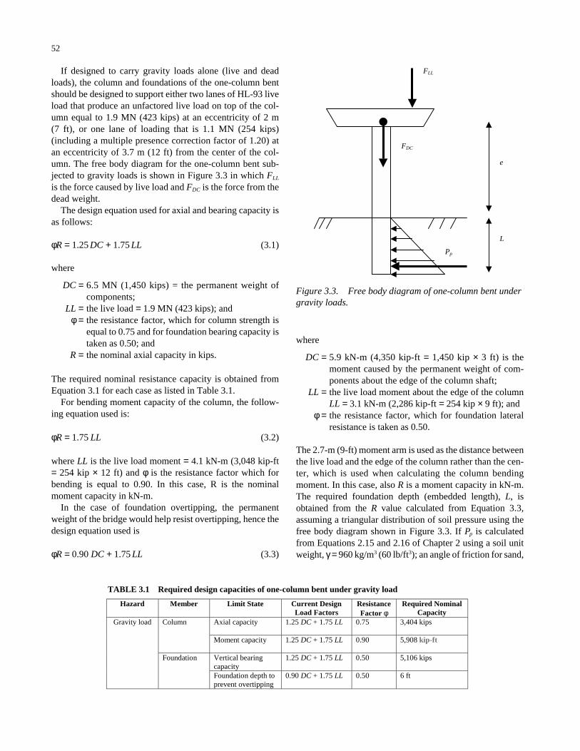
52

If designed to carry gravity loads alone (live and deadloads), the column and foundations of the one-column bentshould be designed to support either two lanes of HL-93 liveload that produce an unfactored live load on top of the col-umn equal to 1.9 MN (423 kips) at an eccentricity of 2 m (7 ft), or one lane of loading that is 1.1 MN (254 kips)(including a multiple presence correction factor of 1.20) atan eccentricity of 3.7 m (12 ft) from the center of the col-umn. The free body diagram for the one-column bent sub-jected to gravity loads is shown in Figure 3.3 in which FLL

is the force caused by live load and FDC is the force from thedead weight.

The design equation used for axial and bearing capacity isas follows:

φR = 1.25 DC + 1.75 LL (3.1)

where

DC = 6.5 MN (1,450 kips) = the permanent weight ofcomponents;

LL = the live load = 1.9 MN (423 kips); andφ = the resistance factor, which for column strength is

equal to 0.75 and for foundation bearing capacity istaken as 0.50; and

R = the nominal axial capacity in kips.

The required nominal resistance capacity is obtained fromEquation 3.1 for each case as listed in Table 3.1.

For bending moment capacity of the column, the follow-ing equation used is:

φR = 1.75 LL (3.2)

where LL is the live load moment = 4.1 kN-m (3,048 kip-ft= 254 kip × 12 ft) and φ is the resistance factor which forbending is equal to 0.90. In this case, R is the nominalmoment capacity in kN-m.

In the case of foundation overtipping, the permanentweight of the bridge would help resist overtipping, hence thedesign equation used is

φR = 0.90 DC + 1.75 LL (3.3)

where

DC = 5.9 kN-m (4,350 kip-ft = 1,450 kip × 3 ft) is themoment caused by the permanent weight of com-ponents about the edge of the column shaft;

LL = the live load moment about the edge of the columnLL = 3.1 kN-m (2,286 kip-ft = 254 kip × 9 ft); and

φ = the resistance factor, which for foundation lateralresistance is taken as 0.50.

The 2.7-m (9-ft) moment arm is used as the distance betweenthe live load and the edge of the column rather than the cen-ter, which is used when calculating the column bendingmoment. In this case, also R is a moment capacity in kN-m.The required foundation depth (embedded length), L, isobtained from the R value calculated from Equation 3.3,assuming a triangular distribution of soil pressure using thefree body diagram shown in Figure 3.3. If Pp is calculatedfrom Equations 2.15 and 2.16 of Chapter 2 using a soil unitweight, γ =960 kg/m3 (60 lb/ft3); an angle of friction for sand,

Pp

e

L

FDC

FLL

Figure 3.3. Free body diagram of one-column bent undergravity loads.

TABLE 3.1 Required design capacities of one-column bent under gravity load

Hazard Member Limit State Current Design Load Factors

Resistance Factor φ

Required Nominal Capacity

Axial capacity

1.25 DC + 1.75 LL 0.75 3,404 kips Column

Moment capacity

1.25 DC + 1.75 LL 0.90 5,908 kip-ft

Vertical bearing capacity

1.25 DC + 1.75 LL 0.50 5,106 kips

Gravity load

Foundation

Foundation depth to prevent overtipping

0.90 DC + 1.75 LL 0.50 6 ft

φs = 35°; and a column diameter, D = 1.8 m (6 ft); then L isfound by setting R = Pp L /3. Knowing R from Equation 3.3,the foundation depth, L, required to resist overtipping can becalculated as L = 1.8 m (6 ft).

Table 3.1 summarizes the results of the nominal designcapacities for the column axial force, column bending moment,foundation bearing resistance, and foundation depth for theone-column bent.

Wind Loads

The design of the single-column bridge bent for wind loadin interior regions of the United States uses a design windspeed of 145 km/h (90 mph) as stipulated in the AASHTOLRFD wind maps. The AASHTO LRFD design equation forthe moment capacity of the column when the system is sub-jected to wind is given as follows:

φR = 1.40 WS (3.4)

where R is the required moment capacity of the column andWS is the applied moment. For overtipping about the base ofthe foundation system, the equation used is of the form

φR = 0.90 DC + 1.40 WS. (3.5)

In Equation 3.5, DC is the moment produced by the perma-nent weight about the bottom edge of the column, and WS isthe moment about the base of the column produced by thewind load on the structure.

53

In Equation 3.4, the maximum bending moment in the col-umn occurs at a point located at a distance f below the soilsurface. f corresponds to the point in which the lateral forcePp in the soil is equal to the applied lateral force from thewind. The free body diagram for column bending is illus-trated in Figure 3.4(b). For Equation 3.5, which checks thesafety of the system against overtipping about the base, thefree body diagram is illustrated in Figure 3.4(a).

The forces F1 applied on the superstructure and F2 appliedon the column because of the wind are calculated from theAASHTO LRFD wind pressure equation, which is given asfollows:

(3.6)

where PB is base wind pressure = 0.0024 MPa for beams andVDZ is the design wind velocity at design elevation Z, whichis calculated from

(3.7)

where

V10 = wind velocity above ground level = 145 km/h (90mph) in the case studied herein;

V0 = friction velocity = 13.2 km/h (8 mph) for opencountry;

VB = base wind velocity = 160 km/h (100 mph); andZ0 = friction length = 70 mm for open country.

V VVV

ZZDZ

B=

2 5 0

10

0. ln

P P VD B

DZ=2

25 600,

(a) (b)

H

F1

Pp

e1

F1

f L

FDC

F2 F2

e2

e1

e2

Figure 3.4. Free body diagram of bridge foundation system: (a) free body diagram for a shortpile, dominant failure mode is tipping at base; (b) diagram for a long pile, dominant failuremode is column bending at distance f below soil level.

Using a superstructure depth of 2.4 m (8 ft), the wind forcetransmitted from the superstructure to the column is calcu-lated to be F1 = 140 kN (31.6 kips) applied at a height e1 = 8.8m (29 ft) from the soil surface. The force applied on the sub-structure is F2 = 27 kN (6 kips) at a height e2 = 3.6 m (11.8 ft).For long columns, the point of maximum moment is at f =1.6 m (5.14 ft) below the soil surface. Thus, the moment fromthe wind on the structure WS = 1600 kN (1,180 kip-ft). Thecorresponding nominal design bending moment of 2500 kN-m (1,835 kip-ft) is obtained from Equation 3.4 using aresistance factor φ =0.90.

The results of Equation 3.5 show that the column is ableto resist overtipping simply because of the counteractingeffects of the permanent weight. Thus, the foundation depthis controlled by effects other than the wind load (e.g., theeffect of live load as shown in the previous section). Table3.2 summarizes the wind load design requirements.

Earthquakes

When performing a dynamic analysis in the transversedirection and assuming that the point of fixity for lateraldeformation is 5.5 m (18 ft) below soil level, the effectiveweight of the column above the point of fixity is equal to 747kN (168 kips). In this latter case, the center of mass is 8 m(27 ft) above soil level (= 45 ft from the point of fixity). Fol-lowing common practice in earthquake engineering andassuming a tributary length of 28 m (91.75 ft = 50% of thedistance to other bent and 70% of distance to abutment), thetotal weight from the superstructure and wearing surfaceapplied on one bent adds up to 5360 kN (1,205 kips). Thus,the total weight on one bent is equal to 6800 kN (1,527 kips).This assumes that the lateral connection of the superstructureto the abutments will not break because of the earthquake-induced lateral motions. Notice that the total weight is slightlyhigher than for the gravity load because of the inclusion of theweight of the pile up to the point of fixity. The center of massis calculated to be at 8.2 m (27 ft) above the soil surface.

The inertial forces applied on the bent because of the earth-quake accelerations may be represented as shown in Figure3.5. The point of fixity at a distance Le below the soil surfacecan be calculated as a function of the soil elastic modulus, Es,the foundation depth, L, and the stiffness of the column repre-sented by Ep Ip where Ep is the modulus of the concrete pile andIp is the moment of inertia of the concrete pile. The foundationis assumed to consist of a drilled pile shaft (pile extension) that

54

extends 15 m (50 ft) into the soil. The soil is assumed to havean elastic modulus Es = 69 MPa (10,000 psi) correspondingto moderately stiff sand. The point of fixity of the floatingfoundation can be calculated using the relationship providedby Poulos and Davis (1980) given as follows:

(3.8)

where

Le = the effective depth of the foundation (distance fromground level to point of fixity);

L = the actual depth;e = the clear distance of the column above ground level;

KR = the pile flexibility factor, which gives the relativestiffness of the pile and soil;

IρH = the influence coefficient for lateral force; andIρM = the influence coefficient for moment.

The pile flexibility factor is given as follows:

(3.9)

If the pile is made of 28 MPa (4,000 psi) concrete, then Ep =25 GPa and the diameter of the col-umn being D = 1.8 m (6 ft) result in a moment of inertia Ip =0.55 m4 (63.62 ft4 = πr4/4). Thus, for a pile length of 15 m (50ft), the pile flexibility becomes KR = 0.0037. The charts pro-vided by Poulos and Davis (1980) show that for KR = 0.0037the influence coefficients IρH and IρM are respectively on theorder of 5 and 15. The root of Equation 3.8 produces a ratioLe/L = 0.35, resulting in an effective depth, Le , of 18 ft belowground surface. Thus, the effective total column height untilthe point of fixity becomes H = 13.7 m (45 ft = 27 ft + 18 ft).

The natural period of the column bent can be calculatedfrom

(3.10)

where the column stiffness is given as K = 3Ep Ip /H3 and themass M is the equal to weight 6.8 MN (1,527 kips) dividedby g, the acceleration due to gravity. Given the material andgeometric properties, the natural period of the column isfound to be T = 1.31 sec.

T MK

= 2π

3 600 57 4 000, ksi ,=( )

KE IE LR

p p

s= 4 .

LL

eL

LL

K I eL

Ie eR H M

+

= +( )3 2

1 5 3. ρ ρ

TABLE 3.2 Required design capacities of one-column bent under wind load

Hazard Member Limit State Current Design Load Factors

Resistance Factor φ

Required Nominal Capacity

Column Moment capacity

1.40 WS 0.90 1,835 kip-ft Wind load

Foundation Overtipping

0.90 DC + 1.40 WS 0.50 0 ft

The natural period of the system is used along with Equa-tions 2.17 through 2.19 and Table 2.4 of Chapter 2 to find thespectral accelerations, Sa, for different bridge site locations.The soil is assumed to be of type D. The spectral accelerationscalculated for the 2,500-year return period (2% probability ofexceedance in 50 years) are shown in Table 3.3. The equiva-lent inertial forces, Fi, for nonlinear columns are obtainedusing Equation 3.11:

(3.11)

where

Sa = the spectral acceleration as a function of the acceler-ation due to gravity, g;

W = the weight of the structure; andRm = the response modification factor.

Assuming a response modification factor Rm = 1.50 as spec-ified in the proposed AASHTO LRFD earthquake designspecifications in NCHRP Report 472 (ATC and MCEER,2002), the equivalent inertial forces accounting for columnnonlinearity are calculated as shown in Table 3.3. Using thefree body diagrams of Figure 3.4(b) with F1 = Fi and F2 = 0,the required moment capacities for the bridge column for dif-ferent earthquake sites are given as shown in Table 3.3.

FS WRia

m=

55

Table 3.3 also shows the required foundation depth, L, cal-culated using the free body diagram of Figure 3.4(a). In thiscase, the Rm value used is Rm = 1.0 because rigid body over-tipping is assumed to occur in short columns where the max-imum moment capacity has not been reached yet (i.e., whenthe column’s bending moment is still in the linear elasticrange). For these cases, the required foundation depth, L, isgiven in the last column of Table 3.3.

Note that following common practice, the stiffness and thenatural period of the system are calculated using Equations3.8 and 3.9, which are based on the elastic behavior of thesystem. The design uses Equation 3.11 and the free body dia-gram of Figure 3.4, which are based on ultimate capacity.

Scour

It is herein assumed that the bridge is constructed over a 67-m (220-ft) wide rectangular river channel as shown in Figure3.1. To obtain realistic results for the effect of scour, differentpossible discharge rate data from different small rivers areused, and design scour depths are calculated for each of theseriver discharge rates. The rivers chosen for this analysis con-sist of the following: (1) Schohaire Creek in upstate NewYork, (2) Mohawk River in upstate New York, (3) CuyahogaRiver in northern Ohio, (4) Rocky River in Ohio, and (5) San-dusky River in Ohio. Data on the peak annual discharge ratesfor each of the five rivers were obtained from the USGS web-site. Lognormal probability plots and Kolmogorov–Smirnov(K-S) goodness-of-fit tests showed that the peak annual dis-charge rate, Q, for all five rivers can be reasonably well mod-eled by lognormal probability distributions. The mean of thelog Q and its standard deviation were calculated using a max-imum likelihood estimator. These data are provided in Table2.8 of Chapter 2. Assuming a slope of S0 = 0.2% and a Man-ning roughness coefficient of n = 0.025, the flow depth forthe 100-year flood, ymax, can be calculated along with the cor-responding flow velocity, V, for each of the five rivers, usingEquations 2.22 through 2.28. Assuming a 67-m (220-ft) widerectangular channel and a pier diameter of D = 1.8 m (6 ft),the maximum design scour depth for the one-column bentbridge for each river data is obtained as shown in Table 3.4.

To avoid failure caused by scour, the foundation depthshould be designed for a length, L, greater than or equal tothe design scour depth, Ymax, which is given in Table 3.4.

H

Fi

e

Le L

Figure 3.5. Dynamic analysis model.

TABLE 3.3 Earthquake design requirements for five sites

Site Spectral Acceleration, Sa

Equivalent Inertial Force, Fi

Required Moment Capacity, Mcap

Required Foundation Depth, L

San Francisco 1.15 g 1,171 kips 55,950 kip-ft 86 ft Seattle 0.64 g 652 kips 28,320 kip-ft 66 ft Memphis 0.50 g 510 kips 21,050 kip-ft 59 ft New York 0.17 g 173 kips 6,500 kip-ft 37 ft St. Paul 0.05 g 51 kips 1,670 kip-ft 20 ft

Vessel Collision

The basic bridge configuration shown in Figure 3.1 doesnot allow for the passage of vessels under the bridge span.Hence, a different bridge configuration is assumed to studythe vessel collision problem. For the purposes of this study,the bridge configuration selected is similar to that of the Inter-state 40 (I-40) bridge over the Mississippi River in Memphis,which is fully described in Appendix D. The bridge pier andwater channel configurations are represented as shown in Fig-ure 3.6. USACE provided data on the types of barges thattravel the Mississippi River near Memphis along with theirweights. The data are used along with the model of theAASHTO guide specifications (1991) following the recom-mendations proposed by Whitney et al. (1996) to find therequired design vessel impact force that would produce anominal annual failure rate of AF = 0.001.

The calculations use Equation 2.32 through 2.38, whichare given in Chapter 2. According to the analysis summa-rized in Table 3.5 the design impact force should be HCV = 35

56

MN (7,900 kips). This design impact force is assumed to beapplied at 4.9 m (16 ft) above soil level on a column that has adiameter D = 6.1 m (20 ft). The free body diagram for design-ing the column and foundation capacities is similar to thatdepicted in Figure 3.4, with F1 = 0.0, F2 = HCV, and e2 = 4.9 m(16 ft). Given the very large permanent weight that is appliedon the bent from the large superstructure needed to span theriver channel, the possibility of overtipping because of ves-sel collision is negligibly small. Hence, only two limit statesare investigated for this case: (1) failure of the column inshear, and (2) failure of the column in bending moment.

The design for shear is checked using an equation of theform

φR = 1.00 CV (3.12)

where CV is the vessel collision force CV = HCV = 35 MN(7,900 kips) and is the resistance factor for shear, whichaccording to the AASHTO LRFD should be equal to 0.90 fornormal density concrete. This would result in a required shear

TABLE 3.4 Design scour depth for five rivers

River Q 100-year (ft3/sec)

V (ft/sec)

Y0 - flood depth (ft)

Ymax – design scour depth (ft), one-column bent

Schohaire 78,146 17.81 20.56 17.34 Mohawk 32,747 12.87 11.78 13.99 Sandusky 36,103 13.35 12.52 14.33 Cuyahoga 19,299 10.50 8.45 12.26 Rocky 19,693 10.58 8.56 12.32

2470’

Y0

12’

Bridge Pier

125’ 600’ 245’ 350’

65’

55’

Centers of vessel traffic paths

360’ 176’

20’

Upstream Downstream

Figure 3.6. Profile of river channel for vessel collisions.

column capacity equal to Vcap = 39 MN (8,780 kips). The pointof fixity is found to be at f = 10.5 m (34.5 ft) below the soillevel. Using the free body diagram of Figure 3.4(b) and amoment resistance factor, φ, also equal to 0.90, the requiredcolumn moment capacity is found be equal to Mcap = 464MN-m (342,333 kip-ft). The design requirements for the col-umn subjected to vessel collision are summarized in Table 3.6.

3.1.2 Two-Column Bents

The second design option is for the same bridge super-structure described in Figure 3.1, but where the substructure

57

consists of two bents, each formed by two 1.1-m (3.5-ft)diameter columns spaced at 7.9 m (26 ft) center to center asdescribed in Figure 3.2(a). The clear column height is 6.3 m(20.5 ft) connected by a 1.4-m (4.5-ft) cap carrying six Type-6 AASHTO girders and a 10-in. deck slab plus wearing sur-face. The bent carries the same 12.2-m (40-ft) wide deck witha 0.91-m (3-ft) curb on each side as that of the one-columnbent. The required column capacities are calculated to satisfyeach of the pertinent loads using the current AASHTO LRFDspecifications. Specifically, the required moment capacity iscalculated for the two-column bent when subjected to theeffects of wind loads, earthquakes, and vessel collision forces.The analysis assumes that the bent cap is very stiff compared

TABLE 3.5 Details of calculations of annual failure rates for vessel collisions by flotilla type

Typea Frequency Number of Mean Distances (m) Normalized PGd PAd PCd N*PA*PG*PC

Down-bound columns rows weight(MN) LOA(m)b Bmc d1c d2c d1 d2

AB 91 4 1.9 22.92 18.74 9.45 152.56 176.62 2.04 2.36 0.01 1.77E-04 0.00 0.00 BC 126 5.93 2.05 138.44 44.52 16.11 145.03 184.15 0.55 0.70 0.05 1.77E-04 0.00 0.00 BD 1 5.11 2.93 128.28 45.35 16.49 137.39 191.80 0.59 0.83 0.07 1.77E-04 0.00 0.00 CC 79 5.11 2.93 92.63 54.70 12.24 143.62 185.57 0.51 0.66 0.05 1.77E-04 0.00 0.00 DC 35610 5.38 3.21 116.19 59.44 10.67 144.41 184.77 0.45 0.58 0.04 1.77E-04 0.00 0.00 EA 6 5 1 119.22 60.96 7.62 157.73 171.45 0.52 0.56 0.02 1.77E-04 0.00 0.00 EB 6 5 1 124.82 60.96 9.30 156.90 172.29 0.51 0.57 0.02 1.77E-04 0.00 0.00 EC 33026 5.38 3.3 129.44 61.53 10.81 143.71 185.47 0.43 0.56 0.04 1.77E-04 0.00 0.00 FC 1043 4.5 3 209.20 79.81 15.96 137.60 191.58 0.38 0.53 0.05 1.77E-04 0.00 0.00 GC 648 4 2.8 195.75 90.01 16.17 138.91 190.27 0.39 0.53 0.05 1.77E-04 0.00 0.00 GD 19 3.23 2.3 173.97 90.71 16.49 142.58 186.60 0.49 0.64 0.05 1.77E-04 0.00 0.00 HC 17 3.23 2.3 166.98 96.53 16.17 142.95 186.24 0.46 0.60 0.05 1.77E-04 0.00 0.00 Up-bound AB 219 4 1.9 22.60 18.73 9.42 97.73 121.73 1.30 1.63 0.04 1.77E-04 AC 78 4 1.9 72.28 30.30 16.46 91.04 128.41 0.75 1.06 0.08 1.77E-04 BB 4 4 1.9 9.97 35.05 8.84 98.28 121.17 0.70 0.86 0.05 1.77E-04 BC 760 5.93 2.05 147.40 44.40 15.99 90.29 129.16 0.34 0.49 0.05 1.77E-04 1.97E-02 1.43E-04 BD 151 5.11 2.93 138.53 45.35 16.49 82.52 136.93 0.36 0.59 0.08 1.77E-04 1.15E-02 2.57E-05 CC 396 5.11 2.93 159.39 53.79 16.07 83.14 136.32 0.30 0.50 0.07 1.77E-04 1.69E-02 8.45E-05 DC 14698 5.38 3.21 119.36 59.44 10.74 89.43 130.02 0.28 0.41 0.05 1.77E-04 EB 1 5 1 116.89 60.96 9.30 102.03 117.42 0.33 0.39 0.02 1.77E-04 EC 12097 5.38 3.3 131.09 61.62 11.05 88.45 131.01 0.27 0.40 0.05 1.77E-04 2.90E-03 3.01E-04 ED 1 4.5 3 68.03 73.46 17.68 80.16 139.29 0.24 0.42 0.07 1.77E-04 FC 697 4.5 3 193.33 81.43 16.02 82.66 136.80 0.23 0.37 0.06 1.77E-04 1.96E-02 1.36E-04 FD 2 4.5 3 125.15 81.38 17.68 80.16 139.29 0.22 0.38 0.06 1.77E-04 3.20E-03 6.97E-08 GC 2028 4 2.8 197.23 90.03 16.25 83.93 135.52 0.23 0.38 0.05 1.77E-04 1.58E-02 3.10E-04 GD 158 3.23 2.3 145.12 90.71 16.49 87.72 131.74 0.30 0.45 0.06 1.77E-04 HC 73 3.23 2.3 145.11 96.55 15.67 88.66 130.79 0.28 0.42 0.05 1.77E-04 HD 17 2 1 103.57 117.98 21.76 95.80 123.65 0.41 0.52 0.04 1.77E-04

NOTES:(a) The definitions of barge flotilla types are provided in Appendix E (on CRP-CD-30).(b) LOA = length overall of flotilla.(c) These terms are defined in Figure 2.12, shown as x1 and x2.(d) See Section 2.4.5 for definitions of the probabilities PA, PG, and PC.

TABLE 3.6 Required design capacities of one-column bent under vessel collision forces

Hazard Member Limit State Current Design Load Factors

Resistance Factor φ

Required Nominal Capacity

Column Moment capacity

1.00 VC 0.90 342,333 kip-ft Vessel Collision

Column Shearing capacity

1.00 VC 0.90 8,780 kips

58

with the columns. Thus, vertical loads will produce negligi-ble moments in the columns, and only the lateral loads willproduce moments. Because of the presence of the two col-umns, no overtipping is possible, although foundation depthis controlled by the scour requirements. In addition, the col-umn axial capacity and foundation bearing capacity are deter-mined to satisfy the requirements for applied gravity loads.The applied loads and load factors used in the calculationsperformed in this section are those specified by the AASHTOLRFD. A short description of the procedure is provided belowfor each load and limit state analyzed. More details are pro-vided in Appendix C.

Gravity Loads

The weight applied on each bent is calculated as follows:

• Superstructure weight = 156 kN/m (10.67 kip/ft),• Weight of cap beam = 480 kN (109 kips), and• Weight of wearing surface = 35.9 kN/m (2.46 kip/ft).

The weight of the each column above the soil level is 138 kN(31 kips). The analysis of the distributed weights will pro-duce a dead weight reaction at the top of the bent equal to

5400 kN (1,209 kips) from the superstructure plus 480 kN(109 kips) from the cap. These will result in 2900 N (659kips) for each column for a total of 3000 kN (690 kips) percolumn.

If designed to carry vertical loads alone, each column ofthe two-column bent should be designed to support two lanesof HL-93 live load that produce an unfactored live load ontop of the column equal to 188 kN (423 kips) at an eccen-tricity of 1.8 m (6 ft). For one lane of traffic, the live load is1100 kN (254 kips) at an eccentricity of 0.3 m (1 ft). The freebody diagram is shown in Figure 3.7 with the lateral forcesF1 = F2 = 0. In Figure 3.7, e3 denotes the eccentricity of theapplied live load, FLL, relative to the center of a column.Assuming a rigid cap beam compared with the column stiff-ness, the applied moment on the columns caused by verticalloads is small, and the columns need to resist mostly verticalloads. Using design Equation 3.1 results in a required nomi-nal column axial capacity and a nominal foundation bearingcapacity, as are shown in Table 3.7.

Wind Loads

The design of the two-column bridge bent for wind load ininterior regions of the United States uses a design wind speed

e1

FLL

FDC

e3

e2

F2

F1

f

Figure 3.7. Basic free body diagram of two-column bent.

TABLE 3.7 Required design capacities of two-column bent under gravity load

Hazard Member Design Parameter Current Design Load Factors

Resistance Factor φ

Required Nominal Capacity

Column Axial capacity

1.25 DC + 1.75 LL 0.75 1,909 kips Gravity load

Foundation Vertical bearing capacity

1.25 DC + 1.75 LL 0.50 2,864 kips

59

taken as fixed at the base of the effective pile depth and alsofixed on the top of the column because of the presence of thestiff column cap. Thus, the natural period of the bent system,T, is 0.72 sec. The natural period is used to find the inertialforces and the required moment capacities for different earth-quake sites using the same method described in Section 3.1.1for bridges with one-column bent as provided in Equation 3.10,but with K = 12EpIp /L3. Given the natural period, T, the spec-tral accelerations are calculated from Equation 2.17 through2.19 of Chapter 2. The inertial forces are calculated usingEquation 3.11 with a response modification factor Rm = 1.5.The spectral accelerations along with the inertial forces arelisted in Table 3.9 for earthquake data from five different sites.The free body diagram described in Figure 3.7 is used with F1

equal to the inertial force while all other forces are set equal tozero. The required column moment capacities are calculatedas shown in Table 3.9 using a resistance factor, φ =0.90.

Scour

The analysis of the two-column bent for scour followsthe same exact method used for the one-column bent. Theonly difference is the diameter of the column where D = 1.1 m(3.5 ft) is used for the two-column bent rather than the valueD = 1.8 m (6 ft), which is used for the one-column bent. Therequired foundation depths for different river flood data areshown in Table 3.10. The required foundation depth, L, foreach river should then be equal to or greater than the valuesof ymax given in Table 3.10.

Vessel Collision

The vessel collision design force of Hcv = 35 MN (7,900kips) for the two-column bent is calculated following thesame exact procedure described above for the single-columnbent. The free body diagram for determining the maximummoment in the column is as shown in Figure 3.7, with F2 =HCV at e2 = 4.9 m (16 ft) and F1 = FLL = 0. In the case of the

of 145 km/h (90 mph) as stipulated in the AASHTO LRFDwind maps. The free body diagram for the wind analysisproblem is as shown in Figure 3.7 with FLL = 0, F1 = 140 kN(31.6 kips) at e1 = 8.8 m (29 ft), and F2 = 18 kN (3.95 kips)at e2 = 4 m (13 ft). The design column bending moment capac-ity to resist the applied lateral caused by wind and allowingfor a resistance factor of 0.90 and a wind load factor of 1.40is equal to 600 kN-m (440 kip-ft) for each column as shownin Table 3.8. The simplified analysis model assumes fixity atthe top because of the presence of a stiff column cap and atthe base at a distance f = 1.4 m (4.6 ft) below the soil level.

Earthquakes

When performing a dynamic analysis in the transversedirection and assuming that the point of fixity for lateral defor-mation is 3 m (10 ft) below soil level, the effective weight ofthe column above the point of fixity is equal to 200 kN (45kips). In this case, the center of mass is 8 m (27 ft) above soillevel (= 11.3 m or 37 ft from the point of fixity). Followingcommon practice in earthquake engineering and assuming atributary length of 28 m (91.75 ft = 50% of the distance toother bent and 70% of distance to abutment), the total weightof superstructure and wearing surface add up to 5360 kN(1,205 kips) for one bent. This will result in a total weight onone column equal to 2.9 MN (650 kips).

As a first step it is assumed that the foundation consists ofa drilled pile shaft (pile extension) that extends 15 m (50 ft)into the soil. A sensitivity analysis is performed at a laterstage to check other foundation depths. The soil is assumedto have an elastic modulus Es = 10,000 psi corresponding tomoderately stiff sand. As explained in Appendix C, the pointof fixity of the floating foundation can be calculated using therelationship provided by Poulos and Davis (1980) to producea point of fixity Le = 3 m (10 ft) below soil level. Given a clearheight of the column e = 6.2 m (20.5 ft), the effective total col-umn height until the point of fixity becomes 9.3 m (30.5 ft =20.5 ft + 10 ft). For transverse seismic motion, the bent is

TABLE 3.9 Earthquake design requirements for two-column bent usingearthquake data from five sites

Site Sa Spectral Acceleration

Fi Equivalent Inertial Force

Mcap, Required Moment Capacity

San Francisco 1.81 g 784 kips 13,500 kip-ft Seattle 1.19 g 516 kips 8,370 kip-ft Memphis 0.92 g 399 kips 6,260 kip-ft New York 0.32 g 139 kips 1,970 kip-ft St. Paul 0.09 g 39 kips 514 kip-ft

TABLE 3.8 Required design capacities of two-column bent for wind load

Hazard Member Design Parameter Current Design Load Factors

Resistance Factor φ

Required Nominal Capacity

Wind load Column Moment capacity

1.40 WS 0.90 440 kip-ft

vessel collision analysis, the column width is taken as 6.1 m(20 ft) and the clear height of the bent is 46 m (150 ft), whichis the same height as the I-40 bridge over the MississippiRiver described in Appendix D. Because the clear columnheight of 46 m (150 ft) is so much higher than the point ofapplication of the force, which is at 4.9 m (16 ft) above thesoil level, most of the applied load remains in the lower por-tion of the impacted column. The maximum shearing forcein the lower part of the column is calculated to be 0.95 timesthe applied force. Hence, the design shearing capacity shouldbe 37 MN (8,340 kips) using a resistance factor φ =0.90. Thepoint of maximum moment is approximated to be at 10 m (33ft) below the soil surface. Hence, using a resistance factor φ =0.90, the required moment capacity at the base will be 430MN-m (317,000 kip-ft). The required moment and shearcapacities are listed in Table 3.11

3.2 RELIABILITY ANALYSIS FOR EXTREMEEVENTS

The reliability index, β, is calculated in this section forbridges designed to satisfy the current AASHTO LRFD cri-teria for the various extreme load events of interest to thisproject. The purpose is to study the level of bridge structuralsafety provided by the current AASHTO LRFD for each ofthe extreme events. Also, the reliability analysis shows howchanges in the design criteria would affect the safety of bridgesystems. This information will also be used to choose the tar-get reliability indexes that will form the basis for calibratingthe load factors for load combinations. The reliability analy-sis uses the methodology and the statistical models describedin Chapter 2. In this section, the reliability analysis is per-formed for gravity loads consisting of live load and deadloads, for wind loads in combination with the permanent loadswhen applicable, for earthquakes alone, for scour, and for ves-sel collisions. The bridges analyzed have the basic geometriesdescribed in Figures 3.1 and 3.2. Modifications on the basic

60

bridge geometry are assumed in order to allow for barge traf-fic under the bridge and, thus, also to study the reliability undervessel collision.

The reliability calculations are performed using a MonteCarlo simulation. The random numbers were generated usingthe method described by Deng and Lin (2000). This methodhas proven to be more stable and capable of generating largenumbers of independent random variables than are similarroutines provided in commercially available mathematicalpackages. An excessively large number of independent ran-dom variables are needed in this study in which Monte Carlosimulations have to be performed for a relatively large num-ber of random variables and to study probabilities of failureon the order of 10−5 to 10−6 (reliability index, β, up to the rangeof 4.0). Monte Carlo simulations are used rather than a FORMalgorithm because some of the cumulative distributions iden-tified in Chapter 2 (e.g., for earthquake intensities and vesselcollision forces described in Figures 2.4 and 2.13) are givenin discrete forms that render them difficult to implement in aFORM algorithm because of the discontinuities of their slopes.

3.2.1 Reliability Analysis for Gravity Loads

In this section, the reliability index implicit in the AASHTOLRFD design criteria is calculated for bridge columns sub-jected to the effect of live loads in combination with deadloads. Four different limit states are studied:

1. Failure of the column under axial load,2. Failure of the foundation caused by exceedance of bear-

ing capacity,3. Overtipping of a column with a short pile shaft, and4. Failure of a long pile shaft in bending.

For the analysis of the column for overtipping, the soil’scontributions in resisting bending are included using the freebody diagram in Figure 3.3. The failure functions for each of

TABLE 3.10 Design scour depth for five rivers

River Q 100-year (ft3/sec)

V (ft/sec)

Y0 flood depth (ft)

Ymax – design scour depth (ft), two-

column bent Schohaire 78146 17.81 20.56 12.31 Mohawk 32747 12.87 11.78 9.93 Sandusky 36103 13.35 12.52 10.17 Cuyahoga 19299 10.50 8.45 8.70 Rocky 19693 10.58 8.56 8.75

TABLE 3.11 Required design capacities of two-column bent under vessel collision forces

Hazard Member Limit State Current Design Load Factors

Resistance Factor φ

Required Nominal Capacity

Column Moment capacity

1.00 VC 0.90 317,000 kip-ft Vessel Collision

Column Shearing capacity

1.00 VC 0.90 8,340 kips

the four limit states considered for one-column bents aregiven as follows:

Z1 = Pcol − FDC − FLL , (3.13)

Z2 = Psoil − FDC − FLL , (3.14)

(3.15)

Z4 = Mcol − FLLe3. (3.16)

For each limit state, i, failure occurs when Zi is less than orequal to zero. Pcol is the column’s axial capacity, FDC is the deadweight applied on the column, FLL is the live load, Psoil is thesoil’s bearing capacity at the column’s tip, γ is the specificweight of the soil, D is the column diameter, Kp gives theRankine coefficient, L is the foundation depth, e3 is the eccen-tricity of the live load relative to the center of the column, andMcol is the column’s bending moment capacity. All the vari-ables used in Equations 3.13 through 3.16 are considered ran-dom except for the column diameter, D, the eccentricity, e3,and the foundation depth, L. Adjustments to Equations 3.13and 3.14 are made when analyzing the two-column bents tofind the portion of FLL and FDC applied on each column. Thestatistical models used to describe the random variables areprovided in Tables 2.1, 2.2 and 2.3. Specifically, the live loadFLL is composed of time-dependent and time-independentrandom variables and can be represented as follows:

FLL = λLLILLHL93 IIM (3.17)

where

λLL = the live load modeling factor,ILL = the live load intensity coefficient,

HL93 = the AASHTO LRFD live load model, andIIM = the dynamic amplification factor.

All the terms in Equation 3.17 except for HL93 are random withstatistical properties provided in Table 2.3 of Chapter 2. ILL isa time-dependent random variable that varies as a function ofthe return period as described in Equations 2.11 and 2.14.

It is noted that the columns are subjected simultaneouslyto axial compression and bending moment. Thus, the col-umn’s load-carrying capacity is governed by a P-M (axial loadversus moment) interaction curve as shown in Figure 2.2.However, for the sake of simplicity and because reliabilitymodels for the combined behavior of bridge columns are notreadily available, Equations 3.13 through 3.16 treat each effectseparately.

For the one-column bent, the column is first assumed tohave the nominal capacities provided in Table 3.1. The col-umns of the two-column bent are first assumed to have thenominal capacities listed in Table 3.7. In addition, a sensi-tivity analysis is performed to study how the reliability index

ZDK L L F D F e Dp

DC LL3

2

33

2 3 2 2= + − −( )γ

, and

61

for each limit state changes as the nominal capacities are var-ied from the required AASHTO LRFD values of Tables 3.1and 3.7. During the reliability calculations, the resistancebiases, COVs, and probability distribution types listed inTables 2.1 and 2.2 of Chapter 2 are used to model the vari-ables that contribute to resisting the failure in each limit state.

Statistical data for modeling the dead and live loads’effects are described in Section 2.4.1 of Chapter 2. The biases,COVs, and probability distributions of all the random vari-ables that describe the effects of gravity loads are providedin Table 2.3. These values are used as input during the relia-bility calculations. Following the model used by Nowak(1999), the bridge is assumed to carry 1,000 individual heavytruck load events or 67 occurrences of heavy side-by-sidetruck events each day. This would result in 27.4 × 106 singletruck events or 1.825 × 106 side-by-side events in a 75-yeardesign period. The 75-year design period is used in this reportto remain compatible with the AASHTO LRFD specifications.Equation 2.14 with m = 27.4 × 106 or 1.825 × 106 is used toobtain the probability distribution of the maximum live loadintensity in 75 years given the probability distribution for oneevent as listed in Table 2.3. The reliability calculations alsoaccount for the modeling factor and the dynamic amplificationfactors. Only the live load intensity is considered to be time-dependent. All the other variables are time-independent in thesense that they are not affected by the 75-year design period.During each cycle of the Monte Carlo simulation, the worstof the one-lane loading or the two-lane loading is used as thefinal load applied on the bridge structure.

The results of the reliability analysis for the four limitstates considered are presented in Figures 3.8 through 3.11for the two- and one-column bents. The figures give the reli-ability index, β, for each limit state as a function of the nom-inal capacity of the column. The abscissas are normalizedsuch that a value of 1.0 indicates that the column is designedto exactly satisfy the requirements of the AASHTO LRFDspecifications for the limit state under consideration. Therequired nominal design capacities for the columns under theeffect of gravity loads are listed in Tables 3.1 and 3.7 forthe one- and two-column bents. Thus, a value of 1.0 for thefailure of the column under axial load (i.e., the first limitstate) means that the column analyzed has a nominal capac-ity Pcap equal to the AASHTO LRFD required design capac-ity or Pcap = Pdesign = 15 MN (3,404 kips). A value of 1.1 indi-cates that the capacity is 10% higher than the required designcapacity such that Pcap = 16.6 MN (3,744 kips).

The steepness of the slope of each curve gives an assess-ment of the cost implied when an increase in the reliabilityindex is desired. For example, a steep positive slope wouldindicate that large increases in the reliability index could beachieved as a result of small increases in the member capac-ities while a shallow positive curve would indicate that largeincreases in the member capacities would be required toachieve small increases in the reliability index.

The results in Figure 3.8 for the columns under axial loadshow that the current AASHTO LRFD produces reliabilityindexes of 3.50 for the two-column bent and 3.32 for the one-column bent. This indicates that the AASHTO LRFD codeproduces reliability index levels close to the 3.5 target beta setby the AASHTO LRFD code writers for columns under axialcompression even though this particular limit state was notspecifically considered during the calibration of the AASHTOLRFD specifications (Nowak, 1999). The figure also shows

62

that an increase in column capacity of 10% (Pcap /Pdesign = 1.1)would result in an average reliability index on the order of3.90. This indicates that improvement in the reliability indexcan be achieved with relatively small increases in columnaxial capacities.

The results for the failure of the soil bearing capacity areillustrated in Figure 3.9. These results show that the currentAASHTO LRFD produces reliability indexes of 2.53 for thetwo-column bent and 2.47 for the one-column bent, which

Reliability index for axial capacity under DC and LL (column)

-1

-0.5

0

0.5

1

1.5

2

2.5

3

3.5

4

4.5

0.70.60.5 0.8 0.9 1.0 1.1 1.2

Pcap/Pdesign(for one column 1.0 is 3,404 kips, for two column 1.0 is 1,909 kips)

Bet

a

one column

two column

Figure 3.8. Reliability of concrete columns under axial load due to gravity.

Reliability index for vertical bearing capacity under DC and LL (foundation)

0.5

1

1.5

2

2.5

3.5

3

0.4 0.80.6 1 1.2 1.61.4 1.8

Pcap/Pdesign(for one column 1.0 is 5,106 kips, for two column 1.0 is 2,864 kips)

Bet

a

one column

two column

Figure 3.9. Reliability of foundation bearing capacity under axial load due to gravity.

indicates that the current code produces lower reliability lev-els for foundation design than for the design of structural ele-ments despite the higher resistance factor of 0.50 used for thedesign of foundations. This is due to the high level of uncer-tainty associated with current methods for designing founda-tions and in estimating soil properties. The data are applica-ble to the models described by Poulos and Davis (1980). Itshould be noted that there are several different methods usedin current practice for the design of foundations. These willproduce different reliability indexes depending on the biasesand implicit safety factors included when the methods aredeveloped. NCHRP Project 12-55, entitled “Load and Resis-tance Factors for Earth Pressures on Bridge Substructuresand Retaining Walls,” is addressing some of these issues.Figure 3.9 shows that an increase in foundation bearing capac-ity of 50% (Pcap/Pdesign = 1.5) would result in an average reli-ability index on the order of 3.0 when Pdesign is calculatedbased on the Poulos and Davis method (1980). A much higherincrease would be required to achieve a reliability index of3.50. Hence, increases in the reliability indexes for bridgefoundations would require large increases in the foundationdepths and sizes because of the relative shallowness of thereliability index curve.

Figures 3.8 and 3.9 also show that the reliability indexes forthe two- and one-column bents are reasonably similar despitethe differences in bent configurations and column sizes.

Figure 3.10 illustrates how the reliability index againstfoundation overtipping for one-column bents varies with foun-dation depth. The figure shows that if the foundation is built toa depth of L = 1.8 m (6 ft) as required using current AASHTOLRFD design standards along with the Broms method forfoundation analysis as described in Poulos and Davis (1980),the reliability index against overtipping is then equal to 3.58.

63

The reliability analysis is based on the free body diagram ofFigure 3.3 and the random variables associated with soilresistance listed in Table 2.2.

It is noticed that doubling of the foundation depth from 1.8m to 3.7 m (6 ft to 12 ft) would result in increasing the relia-bility index to 4.73. The higher reliability index for foundationovertipping compared with that for foundation bearing capac-ity is due to the fact that the Broms method has an implicit biasof about 1.50, as reported by Poulos and Davis (1980). On theother hand, the model proposed by Poulos and Davis (1980)for calculating the ultimate pile shaft bearing capacity forvertical load is not associated with any bias. The differencesemphasize the need to develop more consistent reliability-based models for bridge foundation design. As mentioned ear-lier, NCHRP Project 12-55 is addressing some of these issues.The last failure mode considered for gravity loads only is thefailure of the one-column bent because of bending. Althoughthe live load eccentricity of the one-column bent is relativelysmall and the column will mostly behave as a member underaxial loading, the possibility of bending failures is consideredin this section producing the results presented in Figure 3.11.These results will be used in subsequent sections when study-ing the combination of live loads and other lateral loads thatwill produce high bending moments. If the column is designedto resist the applied moment produced because of the eccen-tricity of the live load, then the AASHTO LRFD specificationsrequire a nominal moment capacity Mcap = 8 MN-m (5,908kip-ft), as shown in Table 3.1. According to Figure 3.11, sucha moment capacity would produce a reliability index of β =3.71. This value is higher than the βtarget = 3.5 used to cali-brate the AASHTO LRFD and is also higher than the valueobserved in Figure 3.8 for column axial capacity. The differ-ence is partially due to the fact that the dead load does not

Reliability index for overtipping of one column under DC and LL

2.5

3

3.5

4

4.5

5

0.4 0.6 0.8 1.21 1.4 1.6 1.8 2

L/L design(1.0 is 6 ft)

Bet

a

Figure 3.10. Reliability for foundation overtipping caused by live and dead loads.

contribute in either resisting or increasing the bendingmoment in one-column bents. The slope of the reliabilityindex curve shows that an increase in moment capacity by10% would produce a reliability index equal to 4.28 (i.e., anincrease in beta of more than 0.57).

The results presented in Figures 3.8 through 3.11 furtherillustrate that, based on the data assembled in Chapter 2, theAASHTO LRFD specifications have achieved a reasonablyuniform reliability index close to the target value of 3.5 forstructural members subjected to gravity loads. The reliabil-ity indexes for foundation design, however, greatly dependon the design methodology followed. Several different foun-dation design methodologies are used in practice that wouldrequire different safety factors to achieve a uniform reliabil-ity level. NCHRP Project 12-55 is currently addressing theissue of the foundation safety and the calibration of resistancefactors for bridge foundation design. The slopes of the relia-bility index curves demonstrate that by increasing the struc-tural properties of the bridge columns by 10%, a relativelylarge increase in the reliability index on the order of 0.40 to0.60 is achieved. On the other hand, very large increases in thefoundation capacities are required to effect small increases inthe reliability index values associated with column overtip-ping or foundation bearing failures.

The results shown in Figures 3.8 through 3.11 show the reli-ability index values calculated for member failure. When thecolumn in a single-column bent fails, it leads to the failure ofthe whole system. On the other hand, when one member of amulticolumn bent system fails in bending, the presence of duc-tility and redundancy will help the system redistribute the loadto provide additional reserve strength. In this case, systemfailure will occur at a higher load. Failures in shear or com-

64

pression do not provide much ductility. Because under grav-ity load the failure of multicolumn bents is primarily due toaxial compression and soil-bearing capacity rather than dueto bending, all types of bents subjected to gravity loads willhave no redundancy.

3.2.2 Reliability Analysis for Wind

The reliability analysis of the one-column and two-columnbents under wind loads is also executed using the modeldescribed in Chapter 2 and using the free body diagrams ofFigures 3.4 and 3.7 with the live load FLL = 0. Referring toFigure 3.4(b), the failure function for column bending in theone-column bent can be represented by an equation of thefollowing form:

(3.18)

where

Mcol = the column bending moment capacity,FWL1 = the wind load on the superstructure,FWL2 = the wind load on the column,

γ = the specific weight of the soil,D = the column diameter,Kp = the Rankine coefficient,

e1 and e2 = the distance of FWL1 and FWL2 from the soil level,f = the distance from the soil level to the point of

maximum moment, and

Z MDK f f

F e f F e f

p

WL WL

5

2

1 1 2 2

32 3

= +

− + + +

col cycγ

λ

[ ( ) ( )]

0

1

2

3

4

5

6

0.4 0.5 0.6 0.7 0.8 0.9 1.0 1.1 1.2 1.3

M cap/M design

Reliability index for moment capacity for one column under live load

(1.0 is 5,908 kip-ft)

Bet

a

Figure 3.11. Reliability index for bending moment of one-column bent.

λcyc = the model of the effect of applying cyclic loadson the foundation.

The distance, f, is calculated by setting the sum of FWL1 +FWL2 = to the lateral load pressure, or

(3.19)

Referring to Equation 3.18, failure occurs when Z5 is lessthan or equal to zero. All the variables used in Equations 3.18and 3.19 are considered random except for the column diam-eter, D, and the eccentricities, e1 and e2. Adjustments toEquations 3.18 and 3.19 are made when analyzing the two-column bents to find the portion of FWL1 and FWL2 applied oneach column. The statistical models used to describe the ran-dom variables are provided in Tables 2.1, 2.2, and 2.7. Specif-ically, the wind load FLW , for either wind on the structure oron the column, is composed of time-dependent and time-independent random variables and can be represented as

FWL = cCp EzG(λVV)2 (3.20)

where

c = an analysis constant,Cp = the pressure coefficient,Ez = the exposure coefficient,G = the gust factor,λV = the statistical modeling factor for wind speeds, andV = the wind speed.

32

2

1 2γDK f

F FpWL WL= +

65

All the terms in Equation 3.20 are random with statisticalproperties provided in Table 2.6 of Chapter 2. The windspeed, V, is a time-dependent random variable that varies asa function of the return period as described in Equations 2.11and 2.14. Mean and COV values of wind speed at differentinterior sites throughout the United States are provided inTable 2.7 for the annual maximum winds and the 50-yearmaximum wind.

The reliability analysis is performed in this section tostudy the safety of bridge columns in bending caused by theeffect of wind alone. The return period used is 75 years inorder to remain compatible with the AASHTO LRFD crite-ria. Notice that Equation 3.18 does not include the effect ofdead loads. Only the bending in the column failure mode isconsidered because preliminary calculations performed inthis study have indicated that the safety of the one-columnbent against overtipping is very high and thus overtipping ofone-column bents because of wind loads is not considered inthis report.

The results of the reliability index calculations for the fail-ure of one column in bending are illustrated in Figure 3.12 forthe one-column bent and Figure 3.13 for the two-columnbents. The calculations are effected for different wind datacollected by Simiu, Changery, and Filliben (1979) and sum-marized by Ellingwood et al. (1980) at seven sites within theinterior of the United States. The results show that bridgestructures designed to satisfy the current AASHTO LRFDspecifications for wind loads (i.e., for Mcap/Mdesign = 1.0) pro-duce an average reliability index value from all the sites ana-lyzed equal to 3.07 for the one-column bent and 3.17 for thetwo-column bent. However, the variability of the results for

Reliability index for moment capacity of one-column bent

0

0.5

1

1.5

2

2.5

3

3.5

4

4.5

0.4 0.6 0.8 1 1.2 1.4 1.6

M cap/M design(1.0 is 1,835.4 kip-ft)

Bet

a

Baltimore,MDDetroit,MISt.Louis,MOAustin,TXTucson,AZRochester,NYSacramento,CA

Figure 3.12. Reliability index for bending moment of one-column bent under wind loads.

different sites is large: the range of the reliability index is from2.41 to 3.92 for one-column bents and from 2.51 to 4.00 fortwo-column bents. This large spread in β is due to the factthat the ASCE-7 design wind speed maps that are adopted byAASHTO use a common design wind of V = 145 km/h (90 mph) for all interior regions; the actual data collected(see Table 2.7) show a large range of values for the meanmaximum winds and their COVs. It is herein recommendedthat future wind maps account for the different wind speedsobserved in different regions.

The results shown for the 7.6-m (25-ft) high bridge pro-duce low applied moments from the wind load as comparedwith the moments caused by the effect of live load. Thus, asensitivity analysis is performed to study the effect of chang-ing the bridge height on the reliability of the bridge column.The results for failure of the one-column bent in bending areshown in Figure 3.14 for different column bents with heightsvarying between 7.6 m and 23 m (25 ft and 75 ft). The resultsillustrate that column height does not significantly affect thereliability index of bridges for the failure mode in bendingalthough a small drop in the reliability index is observed asthe column height increases. The drop in β between theheights of 7.6 m and 23 m (25 ft and 75 ft) is generally lessthan 0.30 such that the average reliability index from the threesites studied—namely St. Louis, Sacramento, and Austin—reduces from a value of 3.13 to an average value of 2.87. TheMdesign values used to normalize the abscissa of the curveshown in Figure 3.14 are the nominal bending moment capac-ities required for exactly satisfying the current AASHTOLRFD criteria. The drop in β is primarily due to the uncer-tainty in identifying the location of the point of maximum

66

moment, f, calculated from Equation 3.19. The value of f ishighly uncertain because of the uncertainty in the soil prop-erties and the modeling of the soil capacity to resist lateralforces. The drop in the reliability index caused by increasesin column height is clearly less significant than the differenceobserved in the effects of site variations in wind speeds onthe reliability index.

The results illustrated in Figures 3.12 through 3.14 show thereliability index values calculated for member failure. Whenthe column in a single-column bent fails, it leads to the failureof the whole system. On the other hand, when one member ofa multicolumn bent system fails in bending, the presence ofductility and redundancy will help the system redistribute theload to provide additional reserve strength. In this case, systemfailure would occur at a higher load. Liu et al. (2001) haveshown that typical two-column bent systems formed by pileextensions subjected to lateral loads provide an additionalreserve strength equal to 15% higher than the strength of onecolumn. Using a system capacity ratio of 1.15 with a COV of8% (as described in Table 2.1 for unconfined columns) wouldlead to higher system reliability index values as compared withthose of one column. Figure 3.15 illustrates the differencebetween the reliability indexes for one column versus for thetwo-column bent system. The wind data used as the basis ofthe calculations are from the St. Louis site. The results showan increase from the 3.16 reliability index for one column to avalue of 3.40 for the two-column system, or an increase ofabout 0.24. Higher increases in the reliability index would beexpected if the concrete columns are highly confined becauseof the effect of the higher ductility levels associated withconfined columns.

Reliability index for moment capacity of column in two-column bent

0

0.5

1

1.5

2

2.5

3

3.5

4

4.5

5

0.4 0.6 0.8 1 1.2 1.4 1.6

M cap/M design(1.0 is 440 kip-ft)

Bet

a

Baltimore,MDDetroit,MISt.Louis,MOAustin,TXTucson,AZRochester,NYSacramento,CA

Figure 3.13. Reliability index for bending moment in two-column bent under wind loads.

67

Reliability index for the check of bent under wind load (one column)

0.5

1

1.5

2

2.5

3

3.5

4

4.5

0.4 0.6 0.8 1.21 1.4 1.6

M cap/M design(for 25ft, 1.0 is 1835 kip-ft, for 50 ft, 1.0 is 4216 kip-ft, for 75ft 1.0 is 7613 kip-ft)

Bet

a

St.Louis,MO (25 ft)St.Louis,MO (50 ft)St.Louis,MO (75 ft)Austin,TX (25 ft)Austin,TX (50 ft)Austin,TX (75 ft)Sacramento,CA (25 ft)Sacramento,CA (50 ft)Sacramento,CA (75 ft)

Figure 3.14. Reliability index for bending moment in one-column bent of different height underwind loads.

Reliability index for two column under wind load alone (St. Louis)

0

0.5

1

1.5

2

2.5

3

3.5

4

0.4 0 .5 0.6 0 .7 0.8 0 .9 1 1 .1 1.2 1 .3M cap/M design

(1.0 is 440 kip-ft)

Bet

a

member capacity

system capacity

Figure 3.15. Comparison of system reliability to member reliability for two-column bent under windload.

3.2.3 Reliability Analysis for Earthquake Alone

The reliability analysis of the one-column and two-col-umn bents under earthquakes is also executed using themodel described in Chapter 2 and using the free body dia-grams of Figures 3.4 and 3.7 with the live load of FLL = 0.For the case of earthquakes, two limit states are considered:(1) the bending of the columns of one- and two-columnbents because of lateral inertial forces and (2) the overtip-ping of the one-column bent. Referring to Figure 3.4(a) and(b), the failure functions for column bending in the one-column bent can be represented by an equation of the fol-lowing form:

(3.21)

where

Mcol = the column bending moment capacity,FEQ = the equivalent earthquake lateral load on the column,

γ = the specific weight of the soil,D = the column diameter,Kp = the Rankine coefficient,e1 = the distance of FEQ from the soil level,f = the distance from the soil level to the point of max-

imum moment, andλcyc = the model of the effect of cyclic loading on the

foundation.

The distance f is calculated by setting the equivalent lateralearthquake load, FEQ, equal to force, Pp, of Figure 3.4 pro-duced from the earth pressure.

Based on Figure 3.4(a), the failure equation for overtip-ping can be represented as follows:

(3.22)

where L is the depth of the foundation. Notice that Equation3.22 does not consider the counter effects of the dead weights.This is because it is herein assumed that vertical accelera-tions caused by the earthquake may significantly reduce thecontributions of the dead weight in resisting the risk forovertipping.

Referring to Equations 3.21 and 3.22, failure occurs wheneither Z6 or Z7 are less than or equal to zero. All the variablesused in Equations 3.21 and 3.22 are considered randomexcept for the column diameter, D; the eccentricity, e1; andfoundation depth, L. The statistical models used to describethe random variables are provided in Tables 2.1, 2.2, and 2.6.Specifically, the equivalent lateral earthquake load, FEQ, iscomposed of time-dependent and time-independent randomvariables and can be represented as follows:

(3.23)F C S t T AWREQ EQ a

m= ′ ′λ ( )

ZDK L L F e Lp

EQ7

2

13

2 3= − +

γλ cyc ( )

Z MDK f f

F e fpEQ6

2

13

2 3= + − +col cyc

γλ ( )

68

where

λEQ = an analysis modeling factor;C′ = the spectrum’s modeling factor;

Sa( ) = the spectral acceleration calculated as a function ofthe calculated nominal period, T;

t′ = the period’s modeling factor;A = the earthquake intensity in terms of the ground

acceleration, g;W = the weight of the structure; andRm = the response modification factor.

When studying overtipping, the response modification factoris Rm = 1.0, and it is deterministic. For column bending, Rm israndom. The variables λEQ, C′, and t′ are also random. W isassumed to be deterministic although the uncertainties inestimating W are considered in λEQ as well as in t′. The earth-quake intensity, A, is the only time-dependent random vari-able that varies as a function of the return period, as isdescribed in Equations 2.11 and 2.14. The probability distri-bution of A is described in Figure 2.4 for five different sites.The probability of exceedance curves of Figure 2.4 are forthe annual maximum earthquake intensity. The calculationsperformed in this report are executed for a 75-year designperiod in order to remain consistent with the AASHTO LRFDspecifications.

The reliability analysis of one-column bent and two-columnbent bridges has been performed using data from the five dif-ferent sites listed in Table 2.4 and Figure 2.4. Figures 3.16and 3.17 show the reliability index for the bending failurelimit state for each of the five sites as a function of the col-umn moment capacity for the one-column bent and the two-column bent, respectively. The abscissa of the plot is normal-ized such that a ratio of 1.0 indicates that the bridge is designedto exactly satisfy the proposed NCHRP Project 12-49 require-ments [ATC and MCEER, 2002] with a nominal responsemodification factor Rm = 1.5. The design column momentcapacities and foundation depths required to resist overtip-ping are provided in Tables 3.3 and 3.9 for five different siteconditions. For the purposes of this study, the bridges are sub-jected to earthquake input motions similar to those expectedin San Francisco, Seattle, St. Paul, New York, or Memphis.The reliability analysis is then performed for each bridge con-figuration and for each of the five site data assuming a 75-yeardesign life. The object is to verify whether the proposedNCHRP Project 12-49 specifications would provide reason-ably uniform reliability levels for any site within the UnitedStates.

Figure 3.16 shows that the proposed NCHRP Project 12-49specifications using a nominal response modification factorof Rm = 1.5 will produce a reliability index, β, that variesbetween 2.56 and 2.88. The average from the five sites is equalto 2.78. If a response modification factor of Rm = 1.0 is used(such as proposed for columns with hinges that cannot beinspected), then the reliability indexes will have an averagevalue of 3.00 with a range of 2.80 to 3.16. These values canbe observed in Figure 3.16 for an Mcap/Mdesign ratio of 1.50

because changing the nominal response modification factorwill result in increasing the moment capacity by the sameratio. The small increase in the reliability index caused by the50% change in Mcap reflects the high costs that would berequired to produce only an incremental change in the relia-bility of bridges subjected to earthquakes. This is due to thefact that the uncertainties in estimating the earthquake inten-sities are very high.

69

Figure 3.17 shows that the range of the reliability indexesfor the two-column bent is slightly higher than that of theone-column bent. The average reliability index for the fiveearthquake data is 2.82 with a minimum β equal to 2.70 anda maximum value equal to 2.91. Since member ductility isalready taken into consideration by using the response mod-ification factor, the reliability indexes shown in Figures 3.16and 3.17 are for the complete system.

Reliability index for bending of a one-column bent under EQ load only (depth = 80 ft)

0

0.5

1

1.5

2

2.5

3

3.5

4

0.4 0.6 0.8 1 1.2 1.4 1.6 1.8 2 2.2M cap/M design

Bet

a

S.Francisco

Seattle

St.Paul

New York

Memphis

Figure 3.16. Reliability index for one-column bent under earthquakes.

Reliability index for bending of two-column bent under EQ load only (depth = 80 ft)

0

0.5

1

1.5

2

2.5

3

3.5

4

0.4 0.6 0.8 1 1.2 1.4 1.6 1.8 2 2.2

M cap/M design

Bet

a

S.FranciscoSeattleSt. PaulNew YorkMemphis

Figure 3.17. Reliability index for two-column bent under earthquakes.

The results shown in Figures 3.16 and 3.17 are for a foun-dation depth L = 24 m (80 ft). The effect of the foundationdepth on the bridge safety is illustrated in Figures 3.18 and3.19. Figure 3.18 shows how the reliability index for thebending limit state for the one-column bent varies with foun-dation depth. It is noticed that the effect is negligibly small.This is due to the fact that a shallow foundation would reducethe stiffness of the system, thus increasing its natural period,which in turn leads to lower spectral accelerations and lowermoments in the column. The maximum difference between

70

the reliability indexes for each site is less than 0.03. Simi-larly, it is observed that the depth of the foundation does notsignificantly affect the reliability index for the bending limitstate of the two-column bent. The reliability indexes shownin Figure 3.19 range from a low value of 2.69 to a high of2.95 for all foundation depths and site data.

Unlike what was observed for column bending, the depthof the foundation affects the safety of the column againstovertipping, as is illustrated in Figure 3.20. In Figure 3.20,the reliability index is calculated using the failure function of

Reliability index for bending of two-column bent under EQ load only(M cap/M design=1.0)

0

0.5

1

1.5

2

2.5

3

3.5

4

40 50 60 70 80 90 100 110

Depth of foundation (ft)

Bet

a

S.Francisco

Seattle

St.Paul

New York

Memphis

Figure 3.19. Reliability index for two-column bent under earthquakes for different foundation depths.

Reliability index for bending of one-column bent under EQ load only(M cap/M design=1.0)

0

0.5

1

1.5

2

2.5

3

3.5

40 50 60 70 80 90 100 110

Depth of foundation (ft)

Bet

a

S.Francisco

Seattle

St.Paul

New York

Memphis

Figure 3.18. Reliability index for one-column bent under earthquakes for different foundation depths.

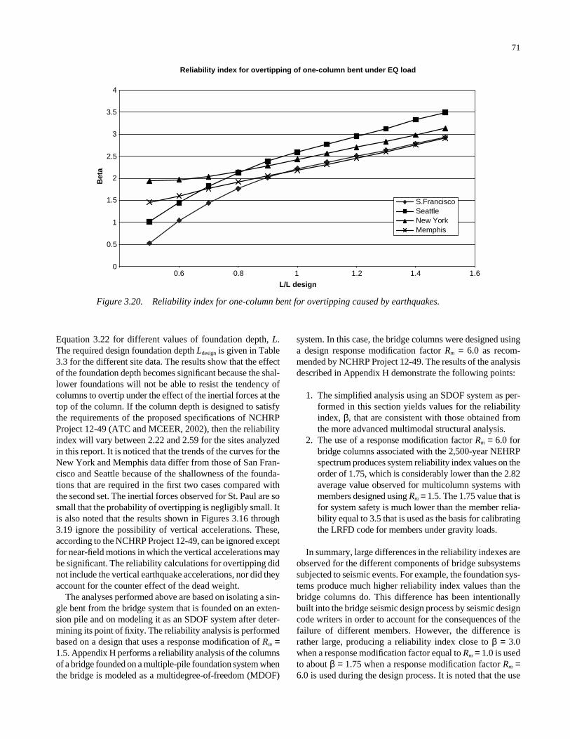
Equation 3.22 for different values of foundation depth, L.The required design foundation depth Ldesign is given in Table3.3 for the different site data. The results show that the effectof the foundation depth becomes significant because the shal-lower foundations will not be able to resist the tendency ofcolumns to overtip under the effect of the inertial forces at thetop of the column. If the column depth is designed to satisfythe requirements of the proposed specifications of NCHRPProject 12-49 (ATC and MCEER, 2002), then the reliabilityindex will vary between 2.22 and 2.59 for the sites analyzedin this report. It is noticed that the trends of the curves for theNew York and Memphis data differ from those of San Fran-cisco and Seattle because of the shallowness of the founda-tions that are required in the first two cases compared withthe second set. The inertial forces observed for St. Paul are sosmall that the probability of overtipping is negligibly small. Itis also noted that the results shown in Figures 3.16 through3.19 ignore the possibility of vertical accelerations. These,according to the NCHRP Project 12-49, can be ignored exceptfor near-field motions in which the vertical accelerations maybe significant. The reliability calculations for overtipping didnot include the vertical earthquake accelerations, nor did theyaccount for the counter effect of the dead weight.

The analyses performed above are based on isolating a sin-gle bent from the bridge system that is founded on an exten-sion pile and on modeling it as an SDOF system after deter-mining its point of fixity. The reliability analysis is performedbased on a design that uses a response modification of Rm =1.5. Appendix H performs a reliability analysis of the columnsof a bridge founded on a multiple-pile foundation system whenthe bridge is modeled as a multidegree-of-freedom (MDOF)

71

system. In this case, the bridge columns were designed usinga design response modification factor Rm = 6.0 as recom-mended by NCHRP Project 12-49. The results of the analysisdescribed in Appendix H demonstrate the following points:

1. The simplified analysis using an SDOF system as per-formed in this section yields values for the reliabilityindex, β, that are consistent with those obtained fromthe more advanced multimodal structural analysis.

2. The use of a response modification factor Rm = 6.0 forbridge columns associated with the 2,500-year NEHRPspectrum produces system reliability index values on theorder of 1.75, which is considerably lower than the 2.82average value observed for multicolumn systems withmembers designed using Rm = 1.5. The 1.75 value that isfor system safety is much lower than the member relia-bility equal to 3.5 that is used as the basis for calibratingthe LRFD code for members under gravity loads.

In summary, large differences in the reliability indexes areobserved for the different components of bridge subsystemssubjected to seismic events. For example, the foundation sys-tems produce much higher reliability index values than thebridge columns do. This difference has been intentionallybuilt into the bridge seismic design process by seismic designcode writers in order to account for the consequences of thefailure of different members. However, the difference israther large, producing a reliability index close to β = 3.0when a response modification factor equal to Rm = 1.0 is usedto about β = 1.75 when a response modification factor Rm =6.0 is used during the design process. It is noted that the use

Reliability index for overtipping of one-column bent under EQ load

0

0.5

1

1.5

2

2.5

3

3.5

4

0.6 0.8 1.21 1.4 1.6

L/L design

Bet

a

S.FranciscoSeattleNew York Memphis

Figure 3.20. Reliability index for one-column bent for overtipping caused by earthquakes.

of a response modification Rm = 1.0 implies a design basedon the elastic behavior of members while a value of Rm = 6.0accounts for the plastic behavior of bridge columns. Thesedifferences, however, will not affect the results of the cali-bration of load factors for combinations of extreme eventsthat include earthquakes as long as the target reliability levelused during the calibration is based on the reliability indexobtained when earthquakes alone are applied on the bridge.This point will be further elaborated upon in Section 3.3.1.

3.2.4 Reliability Analysis for Scour Alone

The scour model described in Chapter 2 can be used in aMonte Carlo simulation program to find the probability thatthe scour depth in a 75-year period will exceed a given valueyCR. In this case, the failure function is given as follows:

Z8 = yCR − ySC. (3.24)

The scour depth, ySC, for rounded piers set in non-cohesivesoils is calculated from

ln ymax = −2.0757 + 0.6285 ln D + 0.4822 ln y0

+ 0.6055 ln V + ε (3.25)

where

D = the pier diameter,y0 = the flow depth,V = the flow velocity, andε = the residual error.

72

As explained in Chapter 2, D is a deterministic variablebecause the pier diameter can be accurately known evenbefore the actual construction of the bridge; y0 and V are ran-dom variables that depend on Manning’s roughness coeffi-cient, n, and the 75-year maximum discharge rate, which arerandom variables having the properties listed in Table 2.9.Based on the analysis of the residuals affected in AppendixI, ε may be considered to follow a normal distribution withmean equal to zero and a standard deviation equal to 0.406.The flow depth, y0, and velocity, V, are calculated from thegeometry of the channel (which is assumed to be determin-istic), from the Manning roughness coefficient (n), and fromthe hydraulic discharge rate (Q) using the relationships pro-vided in Section 2.4.4 of Chapter 2. In addition, the estima-tion of the discharge rate will be associated with statisticaluncertainties represented by a statistical modeling randomvariable, λQ. The pertinent random variables and their prop-erties are listed in Table 2.9 of Chapter 2. Only the dischargerate, Q, is a time-dependent random variable as it increaseswith longer return periods. Given the cumulative distributionfor the maximum 1-year discharge rate, Q, the probabilitydistribution can be calculated for different return periods usingEquation 2.14. In the calculations performed in this report, a75-year return period is used in order to remain compatiblewith the AASHTO LRFD. The calculations are executed forthe discharge data from the five sites listed in Table 2.8.

The probability that ySC will exceed a critical scour depth,yCR , is calculated for different values of yCR as shown in Fig-ure 3.21 for the one-column pier for hydraulic discharge datacollected from five different rivers. Figure 3.22 gives thesame results for the two-column pier. The differences between

Probability of scour depth exceedance (6-ft-diameter column)

0

0.1

0.2

0.3

0.4

0.5

0.6

0.7

0.8

0.9

1

0 5 10 15 20 25 30 35 40 45 50

scour depth (ft)

Pro

bab

lity

of

exce

edan

ce

SchohaireMohawkSanduskyCuyahogaRocky

Figure 3.21. Probability that actual scour will exceed critical depths for 6-ft-diameter column.

the results of the two figures are due to the influence of thecolumn diameter, D, in Equation 3.25.

Figures 3.23 and 3.24 show the reliability index, β, ver-sus the normalized critical foundation depth such that a fac-tor of 1.0 indicates that the foundation is designed to exactlysatisfy the foundation depth requirement of HEC-18 for eachof the river data considered. The safety of bridges against

73

scour is expressed in terms of the reliability index, β, that isobtained from

Pf = Φ(−β) (3.26)

where, in this case, the probability of failure Pf is the proba-bility that the scour depth, ySC, will exceed the design scour

Probablity of scour depth exceedance (3.5-ft-diameter column)

0

0.1

0.2

0.3

0.4

0.5

0.6

0.7

0.8

0.9

1

0 5 10 15 20 25 30 35 40 45 50

scour depth (ft)

Pro

bab

ility

of

exce

edan

ce

Schohaire

Mohawk

Sandusky

Cuyahoga

Rocky

Figure 3.22. Probability that actual scour will exceed critical depths for 3.5-ft-diameter column.

Reliability index for scour depth exceedance (one-column bent)

-4

-3

-2

-1

0

1

2

3

4

5

0 0.5 1 1.5 2 2.5 3 3.5 4

Ycr/Scour design(1.0 is the scour depth of design)

Bet

a

SchohaireMohawkSanduskyCuyahogaRocky

Figure 3.23. Reliability index for scour at different critical depths for D = 6 ft.

74

pared with the design scour depths as calculated from Equa-tion 2.22 and listed in Tables 3.4 and 3.10.

The results in Tables 3.12 and 3.13 show that the reliabil-ity index, β, implied in current scour design procedures variesfrom about 0.47 to 1.66 with an average value of 1.08. Thesevalues are much lower than β = 3.5, which is the reliabilityindex used as the basis for the calibration of the load factorsfor the combination of live and dead loads in the AASHTOLRFD specifications. Also, the target β = 3.5 is for memberreliability while a foundation failure caused by scour willgenerally lead to the collapse of the complete system. The

depth. Φ is the standard Gaussian cumulative distributionfunction.

The results shown in Figures 3.23 and 3.24 demonstratethat the HEC-18 method provides varying degrees of reliabil-ity for the different river data analyzed. The results of the sim-ulation are also summarized as shown in Tables 3.12 and 3.13for the five rivers. The two tables show the average 75-yeardischarge rate and the COV for the 75-year discharge rate forthe one- and two-column bents. They also show the 75-yearmaximum scour depth along with its COV. These are com-

Reliability index for scour depth exceedance (two-column bent)

-4

-3

-2

-1

0

1

2

3

4

5

0 0.5 1 1.5 2 2.5 3 3.5 4

Ycr /Scour design(1.0 is the scour depth of design)

Bet

a

Schohaire

Mohawk

Sandusky

Cuyahoga

Rocky

Figure 3.24. Reliability index for scour at different critical depths for D = 3.5 ft.

TABLE 3.12 Summary of simulation results for one-column pier

River Average Q75yr (Q for 75 years)

(ft3/sec)

COV of Q75yr

Average ys75

(max. scour depth in 75 yrs)

COV of ys75

Design depth

(ft)

Reliabilityindex, β

Schohaire 85,000 29% 16.3 25% 17.3 0.48 Mohawk 34,000 12% 12.6 21% 14.0 0.73 Sandusky 38,000 18% 12.0 22% 14.3 0.90 Cuyahoga 20,000 16% 8.88 21% 12.3 1.60 Rocky 21,000 19% 8.68 22% 12.3 1.66

TABLE 3.13 Summary of simulation results for two-column pier

River Average Q75yr (Q for 75 years)

(ft3/sec)

COV of Q75yr

Average ys75

(max. scour depth in 75 yrs)

COV of ys75

Design depth

(ft)

Reliability index, β

Schohaire 85,000 29% 11.6 25% 12.3 0.47 Mohawk 34,000 12% 8.95 21% 9.93 0.71 Sandusky 38,000 18% 8.57 22% 10.2 0.99 Cuyahoga 20,000 16% 6.33 21% 8.70 1.57 Rocky 21,000 19% 6.18 22% 8.75 1.65

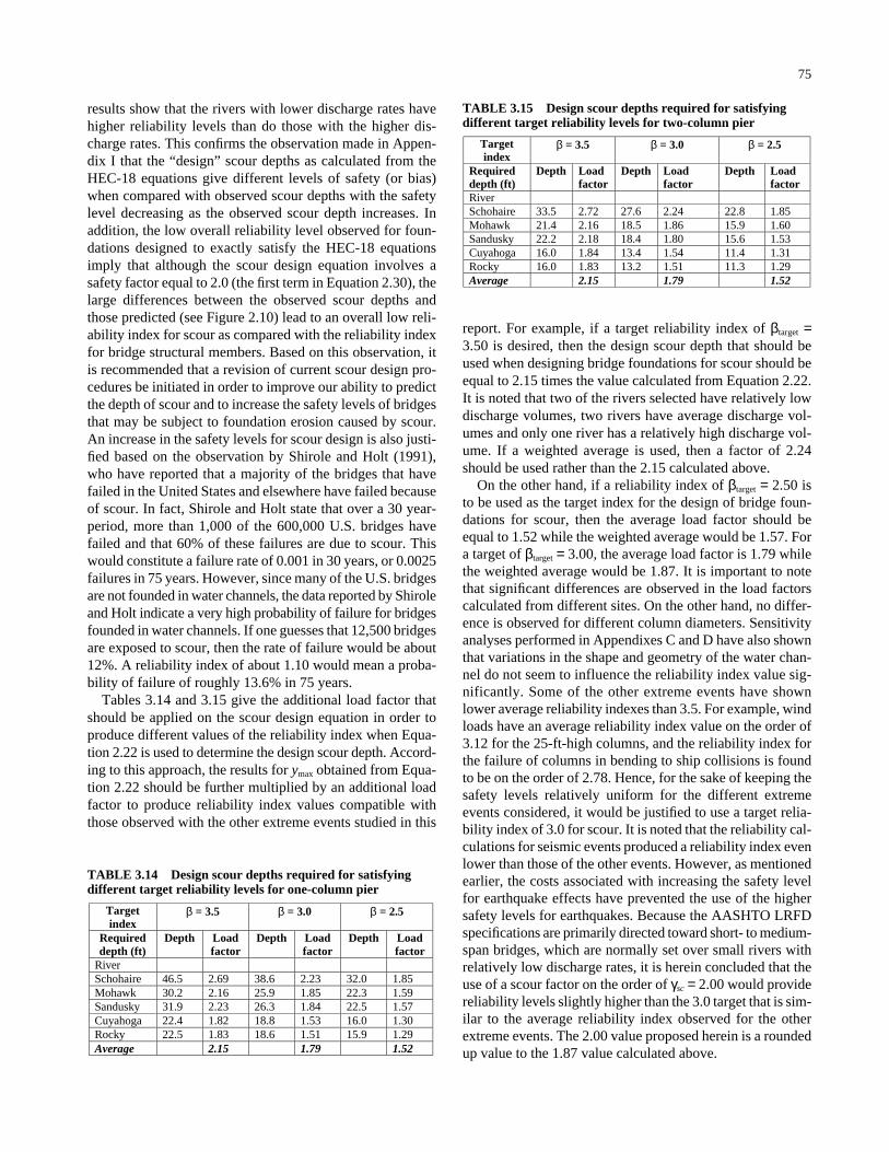
results show that the rivers with lower discharge rates havehigher reliability levels than do those with the higher dis-charge rates. This confirms the observation made in Appen-dix I that the “design” scour depths as calculated from theHEC-18 equations give different levels of safety (or bias)when compared with observed scour depths with the safetylevel decreasing as the observed scour depth increases. Inaddition, the low overall reliability level observed for foun-dations designed to exactly satisfy the HEC-18 equationsimply that although the scour design equation involves asafety factor equal to 2.0 (the first term in Equation 2.30), thelarge differences between the observed scour depths andthose predicted (see Figure 2.10) lead to an overall low reli-ability index for scour as compared with the reliability indexfor bridge structural members. Based on this observation, itis recommended that a revision of current scour design pro-cedures be initiated in order to improve our ability to predictthe depth of scour and to increase the safety levels of bridgesthat may be subject to foundation erosion caused by scour.An increase in the safety levels for scour design is also justi-fied based on the observation by Shirole and Holt (1991),who have reported that a majority of the bridges that havefailed in the United States and elsewhere have failed becauseof scour. In fact, Shirole and Holt state that over a 30 year-period, more than 1,000 of the 600,000 U.S. bridges havefailed and that 60% of these failures are due to scour. Thiswould constitute a failure rate of 0.001 in 30 years, or 0.0025failures in 75 years. However, since many of the U.S. bridgesare not founded in water channels, the data reported by Shiroleand Holt indicate a very high probability of failure for bridgesfounded in water channels. If one guesses that 12,500 bridgesare exposed to scour, then the rate of failure would be about12%. A reliability index of about 1.10 would mean a proba-bility of failure of roughly 13.6% in 75 years.

Tables 3.14 and 3.15 give the additional load factor thatshould be applied on the scour design equation in order toproduce different values of the reliability index when Equa-tion 2.22 is used to determine the design scour depth. Accord-ing to this approach, the results for ymax obtained from Equa-tion 2.22 should be further multiplied by an additional loadfactor to produce reliability index values compatible withthose observed with the other extreme events studied in this

75

report. For example, if a target reliability index of βtarget =3.50 is desired, then the design scour depth that should beused when designing bridge foundations for scour should beequal to 2.15 times the value calculated from Equation 2.22.It is noted that two of the rivers selected have relatively lowdischarge volumes, two rivers have average discharge vol-umes and only one river has a relatively high discharge vol-ume. If a weighted average is used, then a factor of 2.24should be used rather than the 2.15 calculated above.

On the other hand, if a reliability index of βtarget = 2.50 isto be used as the target index for the design of bridge foun-dations for scour, then the average load factor should beequal to 1.52 while the weighted average would be 1.57. Fora target of βtarget = 3.00, the average load factor is 1.79 whilethe weighted average would be 1.87. It is important to notethat significant differences are observed in the load factorscalculated from different sites. On the other hand, no differ-ence is observed for different column diameters. Sensitivityanalyses performed in Appendixes C and D have also shownthat variations in the shape and geometry of the water chan-nel do not seem to influence the reliability index value sig-nificantly. Some of the other extreme events have shownlower average reliability indexes than 3.5. For example, windloads have an average reliability index value on the order of3.12 for the 25-ft-high columns, and the reliability index forthe failure of columns in bending to ship collisions is foundto be on the order of 2.78. Hence, for the sake of keeping thesafety levels relatively uniform for the different extremeevents considered, it would be justified to use a target relia-bility index of 3.0 for scour. It is noted that the reliability cal-culations for seismic events produced a reliability index evenlower than those of the other events. However, as mentionedearlier, the costs associated with increasing the safety levelfor earthquake effects have prevented the use of the highersafety levels for earthquakes. Because the AASHTO LRFDspecifications are primarily directed toward short- to medium-span bridges, which are normally set over small rivers withrelatively low discharge rates, it is herein concluded that theuse of a scour factor on the order of γsc = 2.00 would providereliability levels slightly higher than the 3.0 target that is sim-ilar to the average reliability index observed for the otherextreme events. The 2.00 value proposed herein is a roundedup value to the 1.87 value calculated above.

TABLE 3.14 Design scour depths required for satisfyingdifferent target reliability levels for one-column pier

Target index

β = 3.5 β = 3.0 β = 2.5

Required depth (ft)

Depth Load factor

Depth Load factor

Depth Load factor

River Schohaire 46.5 2.69 38.6 2.23 32.0 1.85 Mohawk 30.2 2.16 25.9 1.85 22.3 1.59 Sandusky 31.9 2.23 26.3 1.84 22.5 1.57 Cuyahoga 22.4 1.82 18.8 1.53 16.0 1.30 Rocky 22.5 1.83 18.6 1.51 15.9 1.29 Average 2.15 1.79 1.52

TABLE 3.15 Design scour depths required for satisfyingdifferent target reliability levels for two-column pier

Target index

β = 3.5 β = 3.0 β = 2.5

Required depth (ft)

Depth Load factor

Depth Load factor

Depth Load factor

River Schohaire 33.5 2.72 27.6 2.24 22.8 1.85 Mohawk 21.4 2.16 18.5 1.86 15.9 1.60 Sandusky 22.2 2.18 18.4 1.80 15.6 1.53 Cuyahoga 16.0 1.84 13.4 1.54 11.4 1.31 Rocky 16.0 1.83 13.2 1.51 11.3 1.29 Average 2.15 1.79 1.52

3.2.5 Reliability Analysis For Vessel CollisionForces

The reliability analysis of the one-column and two-columnbents is also executed for vessel collision forces followingthe model described in Section 2.4.5 of Chapter 2. Using thefree body diagram of Figure 3.4(b) and a force of F2 = FCV

where FCV is the vessel collision force, two limit states areconsidered: (1) the bending of the columns of one- and two-column bents because of lateral collision force and (2) theshear failure of the impacted column. Referring to Figure3.4(b), the failure function for column bending in the one-column bent can be represented by an equation of the form

(3.27)

where

Mcol = the column bending moment capacity,FCV = the vessel collision force on the column,

γ = the specific weight of the soil,D = the column diameter,Kp = the Rankine coefficient,e2 = the distance of FCV from the soil level,f = the distance from the soil level to the point of max-

imum moment, andλcyc = the model of the effect of cyclic loading on the

foundation.

The distance f is calculated by setting the equivalent vesselcollision force, FCV, equal to the force from the soil pressure

Z MDK f f

F e fpCV9

2

23

2 3= + − +col cyc

γλ ( )

76

on the foundation, Pp, of Figure 3.4 produced from the earthpressure. For shearing failure of the column, the failure func-tion is as follows:

Z10 = Vcol − FCV (3.28)

where Vcol is the shearing capacity. The vessel collision forceis calculated from

FCV = x w PB (3.29)

where x is the vessel collision modeling factor, and w is a fac-tor that accounts for the statistical modeling of the calculatedimpact force, PB. All the variables listed in Equations 3.27through 3.29 are random except for the column diameter, D,and the distance, e2. The statistical properties for all the ran-dom variables are listed in Tables 2.1, 2.2, and 2.12. PB is theonly time-dependent variable. The cumulative probabilitydistribution of the maximum value of PB in 1 year is providedin Figure 2.13 of Chapter 2. The calculations executed in thisreport are for a 75-year return period. The probability distri-bution for a 75-year return period for PB is found by usingEquation 2.14.

The results of the reliability calculations are shown in Fig-ures 3.25 and 3.26. As shown in Figure 3.25, the reliabilityindex for shearing failure of the column is calculated to be3.15 when the column is designed to exactly meet the require-ment of the AASHTO LRFD specifications for vessel colli-sions. A 10% increase in the column shearing capacity willincrease the reliability index by 0.35, leading to a reliabilityindex of 3.5. This demonstrates that it would not be very

Reliability index for shear capacity under flotilla collisions

0

0.5

1

1.5

2

2.5

3

3.5

4

4.5

0.50.4 0.6 0.7 0.8 0.9 1 1.1 1.2 1.3 1.4

Shear capacity / Shear design (1.0 is 12,289 kips)

Bet

a

Figure 3.25. Reliability index for shearing failure caused by vessel collisions.

costly to increase the target reliability level for shearing fail-ures caused by vessel collisions. For column bending (seeFigure 3.26), the reliability index is found to be equal to 2.78 if the column is exactly designed to satisfy theAASHTO LRFD specifications. A 10% increase in the col-umn moment capacity will lead to a 0.24 improvement in β.The lower reliability index for moment failures is due to theinherent biases and conservatism implied in the shear designequations.

The reliability calculations executed in this section foreach of the extreme events will be used in Section 3.3 todetermine the target reliability levels and, subsequently, theload factors for the combination of extreme events.

3.3 RELIABILITY ANALYSIS FORCOMBINATIONS OF EXTREME EVENTSAND CALIBRATION OF LOAD FACTORS

This section presents the results of the reliability analysisexecuted for combinations of extreme events. The results arealso used to perform the calibration of the load factors forcombinations of events. Specifically, the section studies thefollowing combinations:

1. Combinations involving live loads:– Earthquakes, EQ, and live loads, LL; – Wind loads, WS, plus live loads, LL; – Scour, SC, and live loads, LL.

2. Combinations involving scour: – Earthquakes, EQ, and scour, SC; – Wind loads, WS, plus scour, SC;

77

– Collision of vessels and scour, SC, in addition to thecase of live load plus scour addressed earlier.

3. Combinations involving vessel collision forces: – Wind loads, WS, plus vessel collision forces, CV;– Wind loads, WS, plus collision of vessels, CV, and

scour, SC.

Because the results obtained in Section 3.2 have shownvery little difference between the reliability indexes of two-column bents and one-column bents when these columnsare designed to satisfy the same AASHTO LRFD specifica-tions, this section will concentrate on studying the reliabilityof one-column bents.

3.3.1 Combination of Earthquakes and LiveLoads (EQ + LL)

The single-column bent described in Figure 3.1 is analyzedto illustrate how the combined effects of earthquake and liveloads will affect the bent’s reliability. The data from the fiveearthquake sites with probability distribution curves describedin Figure 2.4 are used. The live load data are obtained from themodels developed by Nowak (1999) under NCHRP Project12-33 as described in Section 2.4.1 (Table 2.3). The reliabilitycalculations follow the Ferry-Borges model described in Sec-tion 2.5. The following conservative assumptions are made:

• All earthquakes last 30 sec (1/2 min), during which timethe moment at the base of the column remains at itshighest value. The intensity of the earthquake responseis constant as shown in Figure 2.15 for the 1/2-min dura-tion of the earthquake.

Reliability index for moment capacity under ship collision

0

0.5

1

1.5

2

2.5

3

3.5

4

4.5

0.4 0.6 0.8 1 1.2 1.4 1.6

M capacity/M design(1.0 is 342,333 kip-ft)

Bet

a

Figure 3.26. Reliability index for bending failure caused by vessel collisions.

• The number of earthquakes expected in 1 year are 8 forthe San Francisco site data, 2 for Seattle, 0.50 for Mem-phis, 0.40 for New York, and 0.01 for St. Paul. Thismeans that the expected number of earthquakes in a 75-year return period in San Francisco will be 600, 150earthquakes for Seattle, 38 in Memphis, 30 in New York,and 1 in St. Paul.

• The probability distribution of the maximum yearlyearthquake may be used to find the probability distribu-tion for a single event using Equation 2.14.

• The live load model for the applied vertical load has thesame biases as those provided in Table B-16 of Nowak’sreport (1999) for the mean maximum negative momentsof two equal continuous spans. Particularly, the resultsprovided by Nowak for the 80-ft spans are used as thebasis for the calculations. These results show that foreach one-lane loading event, the load effect is on theaverage 0.79 times the load effect obtained from theHL-93 loading configuration of the AASHTO LRFDspecifications for one lane of traffic with a COV of 10%.For two lanes, the average load effect is 1.58 times theeffect of one lane of HL-93 with a COV of 7%. Theseresults assume 1,000 single-lane heavy truck events in1 day and 67 two-lane truck events in 1 day based on theassumptions of Nowak (1999) and Moses (2001).

• Equation 2.11 is used to find the probability distributionof the live load for different return periods. In particu-lar, the live load for a t = 1/2 min period is calculated forcombination with the earthquake load effects when anearthquake is on.

• The effects of each earthquake are combined with theeffects of the 1/2 min live load magnitude and projected toprovide the maximum expected combined load in the 75-year bridge design life period using the Ferry-Borgesmodel described in Section 2.5. The calculations accountfor the cases in which the earthquake occurs with the1/2 min live load and the cases in which the live loadarrives when no earthquake is on (which constitute mostof the time).

• The reliability calculations are executed for a columnbending failure limit state.

• The reliability calculations account for the uncertaintiesassociated with predicting the EQ intensity, estimatingthe bridge response given an EQ intensity, the uncer-tainty in projecting the live load magnitude, and theuncertainty in estimating the column capacities.

• The failure equation for bending of the column underthe combined effect may be represented as follows:

(3.30)

where

Mcol = the column’s moment capacity; γ = the specific weight of the soil;

Z MDK f

MpEQ LL= + − +col

36

3

75γ

,

78

D = the column diameter; Kp = the Rankine coefficient;

f = the distance below the soil level at whichpoint the maximum bending momentoccurs; and

MEQ + LL,75 = the applied moment caused by the com-bined effects of the live load, LL, and theearthquake load, EQ, in a return period ofT = 75 years.

The maximum effect of the combined load can be rep-resented as follows:

(3.31)

where

n1 = the number of earthquakes expected ina 75-year period;

n2 = the number of live loads expected in a1/2 min period;

n3 = the number of live load events expectedin a period equal to 75 years minus thetimes when an earthquake is on (i.e., n3 = number of live load events in 75years − n1 × 1/2 min, which is almostequal to the number of truck events in75 years);

A = the earthquake intensity for one event; ILL = the intensity of the live load for one

event; andcEQ and cLL = the analysis coefficients that convert

the earthquake intensity and the live loadintensity to moment effects (e.g., Equa-tions 3.16 and 3.17 show how to con-vert the intensity of the live load into amoment effect, and Equations 3.22 and3.23 show how to convert the intensityof the earthquake acceleration into amoment effect).

The results of the reliability analysis are provided in Figure3.27 for the San Francisco earthquake data for different valuesof the column capacity to resist applied bending moment. Theresults obtained by considering the reliability of the bridgestructure when only earthquakes are considered—that is, bytotally ignoring the effects of live loads—are also illustrated inFigure 3.27. The plot illustrates how, for this site, the effectsof earthquakes dominate the reliability of the bridge when sub-jected to the combined effects of live loads and earthquakes.The results for the San Francisco site, as well as results for theother sites, are summarized in Table 3.16. As an example, ifthe bridge column is designed to satisfy the proposed revisedAASHTO LRFD specifications (the seismic provisions)

Mc A c I

c IEQ LLn

EQn

LL LL

nLL LL

+ =+

, max

max[ max[ ]]

max[ ]751 2

3

developed under NCHRP Project 12-49 (ATC and MCEER,2002), then the required moment capacity for the drilled col-umn shaft using a 2,500-year earthquake return period and aresponse modification factor equal to Rm = 1.5 will be Mcap =Mdesign = 76 MN-m (55,950 kip-ft). This will produce a relia-bility index (for a 75-year bridge design life) equal to β = 2.60if no live load is considered. If one considers that a live loadmay occur within the 1/2 min when an earthquake is activelyvibrating the bridge column, then the reliability index for the76 MN-m column reduces to β = 2.59. The reduction is small.However, if one wishes to increase the reliability index from2.59 back to the original 2.60, then the moment capacity of thecolumn should be increased. By interpolation, the momentcapacity that will produce a reliability index equal to β = 2.60when both earthquake loads and live loads are consideredshould be Mcap = 77 MN-m (56,840 kip-ft) or an increase of1207 kN-m (890 = 56,840 − 55,950 kip-ft).

The Mdesign value 76 MN-m (55,950 kip-ft) includes theeffect of the resistance factor for bending, φ = 0.90. Themoment calculated from the applied earthquake force is equalto MEQ = 68 MN-m (50,355 kip-ft). Also, the applied liveload from the HL-93 live loading will produce a moment in

79

the column equal to MLL = 4,100 kN-m (3,048 kip-ft). Thelive load factor that should be used for the combination ofearthquakes and live load should be determined such that

φMreq = γEQ MEQ + γLL MLL (3.32)

or

0.90 Mreq = γEQ 68 MN-m + γLL 4100 kN-m.

The calibration of the load combination factor involvesthe determination of the values of γEQ and γLL needed to pro-duce the required column moment capacity Mreq = 77 MN-m(56,840 kip-ft). If the value for γEQ is preset at 1.0, then γLL iscalculated to be equal to 0.26. Many other options are avail-able to reach the required 77 MN-m (56,840 kip-ft). How-ever, in this example, it is assumed that the load factor for themoment obtained from the analysis of the earthquake effectsis always equal to γEQ = 1.0. It is noted that in the examplessolved in this section, the dynamic properties of the bridgesystem—particularly, the mass of the system—are not alteredbecause of the presence of live load. The presence of live

Reliability index for one column under EQ and live load (San Francisco)

2.25

2.5

2.75

3

0.5 0.75 1 1.25 1.5 1.75 2 2.25

M cap/M design(1.0 is 5,5946 kip-ft)

Bet

a

EQ alone

EQ+LL

Figure 3.27. Reliability index for moment capacity under earthquakes plus live loads (San Francisco).

TABLE 3.16 Summary of live load factors for combination of EQ plus LL.

Site Mreq (kip-ft) MEQ MLL γLL for LL+EQ

San Francisco 56,840 50,351 3,048 0.26

Seattle 28,855 25,488 3,048 0.16

Memphis 21,597 18,945 3,048 0.17

New York 7,285 5,830 3,048 0.24

St. Paul 4,826 1,503 3,048 0.93

Average 0.21

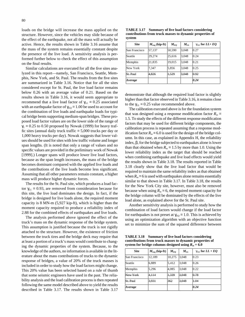
loads on the bridge will increase the mass applied on thestructure. However, since the vehicles may slide because ofthe effect of the earthquake, not all the mass will actually beactive. Hence, the results shown in Table 3.16 assume thatthe mass of the system remains essentially constant despitethe presence of the live load. A sensitivity analysis is per-formed further below to check the effect of this assumptionon the final results.

Similar calculations are executed for all the five sites ana-lyzed in this report—namely, San Francisco, Seattle, Mem-phis, New York, and St. Paul. The results from the five sitesare summarized in Table 3.16. Notice that for all the sitesconsidered except for St. Paul, the live load factor remainsbelow 0.26 with an average value of 0.21. Based on theresults shown in Table 3.16, it would seem appropriate torecommend that a live load factor of γLL = 0.25 associatedwith an earthquake factor of γEQ = 1.00 be used to account forthe combination of live loads and earthquake loads for typi-cal bridge bents supporting medium-span bridges. These pro-posed load factor values are on the lower side of the range ofγL = 0.25 to 0.50 proposed by Nowak (1999) for heavy traf-fic sites (annual daily truck traffic = 5,000 trucks per day or1,000 heavy trucks per day). Nowak suggests that lower val-ues should be used for sites with low traffic volume and longerspan lengths. (It is noted that only a range of values and nospecific values are provided in the preliminary work of Nowak[1999].) Longer spans will produce lower live load factors,because as the span length increases, the mass of the bridgebecomes dominant compared with the applied live loads andthe contributions of the live loads become less significant.Assuming that all other parameters remain constant, a highermass will produce higher dynamic forces.

The results for the St. Paul site, which produces a load fac-tor γLL = 0.93, are removed from consideration because forthis site, the live load dominates the design. In fact, if thebridge is designed for live loads alone, the required momentcapacity is 8 MN-m (5,927 kip-ft), which is higher than themoment capacity required to produce a reliability index of2.88 for the combined effects of earthquakes and live loads.

The analysis performed above ignored the effect of thetruck’s mass on the dynamic response of the bridge system.This assumption is justified because the truck is not rigidlyattached to the structure. However, the existence of frictionbetween the truck tires and the bridge deck may require thatat least a portion of a truck’s mass would contribute to chang-ing the dynamic properties of the system. Because, to theknowledge of the authors, no information is available in the lit-erature about the mass contributions of trucks to the dynamicresponse of bridges, a value of 20% of the truck masses isincluded in order to study how the load factors might change.This 20% value has been selected based on a rule of thumbthat some seismic engineers have used in the past. The relia-bility analysis and the load calibration process is then repeatedfollowing the same model described above to yield the resultsdescribed in Table 3.17. The results shown in Table 3.17

80

demonstrate that although the required load factor is slightlyhigher than that factor observed in Table 3.16, it remains closeto the γLL = 0.25 value recommended above.

The calibration executed above is for the foundation systemthat was designed using a response modification factor Rm =1.5. To study the effects of the different response modificationfactors that may be used for different bridge components, thecalibration process is repeated assuming that a response mod-ification factor Rm = 6.0 is used for the design of the bridge col-umn. In this case, as explained in Appendix H, the reliabilityindex, β, for the bridge subjected to earthquakes alone is lowerthan that obtained when Rm = 1.5 by more than 1.0. Using thelower reliability index as the target that should be reachedwhen combining earthquake and live load effects would yieldthe results shown in Table 3.18. The results reported in Table3.18 clearly show that the live load factor that would berequired to maintain the same reliability index as that obtainedwhen Rm =6 is used with earthquakes alone remains essentiallysimilar to that shown in Table 3.17. In Table 3.18, the resultsfor the New York City site, however, must also be removedbecause when using Rm = 6, the required moment capacity forthe bridge column will be dominated by the effects of the liveload alone, as explained above for the St. Paul site.

Another sensitivity analysis is performed to study how thecombination of load factors would change if the load factorfor earthquakes is not preset at γEQ = 1.0. This is achieved byusing an optimization algorithm with an objective functionset to minimize the sum of the squared difference between

TABLE 3.17 Summary of live load factors consideringcontributions from truck masses to dynamic properties ofsystem

TABLE 3.18 Summary of live load factors consideringcontributions from truck masses to dynamic properties ofsystem for bridge columns designed using Rm = 6.0

Site Mreq (kip-ft) MEQ MLL γ LL for LL+ EQ

San Francisco 57,137 50,590 3,048 0.27

Seattle 29,274 25,616 3,048 0.24

Memphis 21,835 19,015 3,048 0.21

New York 7,347 5,856 3,048 0.25

St. Paul 4,826 1,529 3,048 0.92

Average 0.24

Site Mreq (kip-ft) MEQ MLL γ LL for LL + EQ

San Francisco 12,189 10,275 3,048 0.23

Seattle 6,889 5,412 3,048 0.26

Memphis 5,296 4,085 3,048 0.22

New York 4,114 1,339 3,048 0.78

St. Paul 3,931 362 3,048 1.04

Average 0.24

the results of Equation 3.32 and those of Mreq that are givenin the first column of Table 3.16 when MEQ and MLL areplugged into Equation 3.32 with unknown values of γEQ andγLL. The results show that the square of the difference wouldbe minimized when the combination γEQ = 1.00 and γLL = 0.18is used. This is only slightly different than the results shownin Table 3.16. Hence, for the sake of conservatism, the com-bination γEQ = 1.00 with γLL = 0.25 is recommended for usewhen designing bridges that are susceptible to threats fromthe combined effects of earthquakes and live loads. Pleasenote that these results are very conservative given the previ-ous assumptions that the earthquake is assumed to last for 30sec at its peak value and the live load model follows the con-servative assumptions described by Nowak (1999).

3.3.2 Combination of Wind and Live Loads (WS + LL)

The single-column bent described in Figure 3.1 is ana-lyzed to illustrate how the combined effects of wind and liveloads will affect the bent’s reliability. The wind data fromthree sites—St. Louis, Austin, and Sacramento—are selectedas representative for low, medium, and high wind intensitysites. Table 2.7 of Chapter 2 provides the basic wind inten-sity data for the three sites. The live load data are obtainedfrom the models developed by Nowak (1999) for NCHRPProject 12-33 as described in Section 2.4.1 of Chapter 2(Table 2.3). The reliability calculations follow the Ferry-Borges model described in Section 2.5. The following assump-tions are made:

• All winds last for 4 h, during which time the moment atthe base of the column remains at its highest value. Theintensity of the wind response is constant, as is shownin Figure 2.15 for the 4-h duration of the wind.

• The winds are independent from each other.• Each site is on the average exposed to 200 winds in

1 year. • The probability distribution of the maximum wind speed

follows a Gumbel distribution, which may be used tofind the probability distribution for a single event usingEquation 2.14.

• The live load model assumes that for each one-lane load-ing event, the load effect is on the average 0.79 times theload effect obtained from the HL-93 loading configura-tion for one lane of traffic with a COV of 10%. For twolanes, the average load effect for one event is 1.58 timesthe effect of one lane of HL-93 with a COV of 7%.

• Each site is exposed to 1,000 single-lane heavy truckevents and 67 two-lane truck events in 1 day based onthe assumptions of Nowak (1999) and Moses (2001).

• Equation 2.11 is used to find the probability distributionof the live load for different return periods. In particular,the live load for a 4-h period is calculated for combina-tion with the wind load effects when a windstorm is on.

81

• The effect of each wind is combined with the effect ofthe 4-h live load magnitude and is projected to providethe maximum expected combined load in the 75-yearbridge design life period using the Ferry-Borges modeldescribed in Section 2.5. The calculations account forthe cases in which the wind occurs with the 4-h live loadand the cases in which the live load arrives when nowind is on.

• The reliability calculations are executed for a columnbending failure and column overtipping limit states.

• The reliability calculations account for the uncertain-ties associated with predicting the wind speed intensity,determining the bridge response given a wind load, theuncertainty in projecting the live load magnitude, andthe uncertainty in estimating the column capacities andsoil resistance properties.

• The failure equation for bending may be represented asfollows:

(3.33)

where

Mcol = the column’s moment capacity; γ = the specific weight of the soil;

D = the column diameter; Kp = the Rankine coefficient,

f = the distance below the soil level at whichthe maximum bending moment occurs;and

MWS + LL,75 = the applied moment caused by the com-bined effects of the live load, LL, and thewind load, WS, in a return period of T =75 years.

The maximum effect of the combined load can be rep-resented as follows:

(3.34)

where

n1 = the number of winds expected in a 75-year period (n1 = 200 × 75);

n2 = the number of live loads expected in a4-h period when the wind is on (n2 =167 for one-lane loading and n2 = 11 fortwo-lane loading);

n3 = the number of live load events expectedin a period equal to 75 years minus thetimes when a windstorm is on (i.e., n3 =number of live load events in 75 years −n1 × 4 h);

Mc V c I

c IWS LL

nWS

nLL LL

nLL LL

+ =+[ ]

, max

max max[ ]

max[ ]75

2

1 2

3

Z MDK f

MpWS LL= + − +col

36

3

75γ

,

V = the wind speed for one windstorm; ILL = the intensity of the live load for one

event; and cWS and cLL = the analysis coefficients that convert the

wind speed and the live load intensity tomoment effects (e.g., Equations 3.16 and3.17 show how to convert the intensity ofthe live load into a moment effect, andEquations 3.18 through 3.20 show howto convert the wind speed into a momenteffect).

The effect of wind load on moving trucks is taken into con-sideration during the simulation. However, following thesuggestion of the AASHTO LRFD specifications, the effectof the wind loads on live loads, and the effects of live loadsin combination with wind loads are considered only if thewind speed at 10 m (30.5 ft) is less than 90 km/h (56 mph).For the cases in which the wind speed exceeds 90 km/h (56mph), only the wind load on the structure is considered. Thejustification is that there is no truck traffic under extremewindstorms.

The results of the reliability analysis are provided in Fig-ure 3.28 for the bending limit state of the 7.6-m (25-ft) bridgebent. Figure 3.29 gives the results for overtipping. The dataare presented for the three representative wind sites for com-bination of wind loads and live loads and for wind loadsalone. The effect of the soil in resisting bending and overtip-ping are included in the reliability analysis. Similarly, thecontributions of the permanent load in resisting overtipping

82

are also included. The same calculations are performed for a23-m (75-ft) high pier in order to study the influence ofbridge height on the results. In this case, only the wind datafrom the St. Louis site are used.

The results of the calibration are summarized in Table3.19. As an example, the calibration process follows thislogic: if the 7.6-m (25-ft) bridge column is designed to sat-isfy the AASHTO LRFD specifications, then the requiredmoment capacity for the column will be Mcap = Mdesign = 2.5MN-m (1,835 kip-ft). Choosing Mdesign = 2.5 MN-m (1,835kip-ft) for the Austin wind data will produce a reliabilityindex (for a 75-year bridge design life) equal to β = 3.92 if nolive load is considered. When the bridge column is designedfor live load, then the required moment capacity is Mcap =Mdesign = 8 MN-m (5,917 kip-ft), producing a reliability indexβ = 3.71. If one considers that live loads may occur within the4-h period when a windstorm is acting on the bridge columnas well as when no wind is on, then the reliability index of thecolumn is reduced as shown in Figure 3.28. To increase thereliability index back to the original β = 3.71 obtained forgravity loads alone, the moment capacity of the column shouldbe increased. By interpolation, the moment capacity that willproduce a reliability index equal to β = 3.71 when both windloads and live loads are considered should be Mrequired = 8.2MN-m (6,038 kip-ft) or an increase of 200 kN-m (121 =6,038 − 5,917 kip-ft).

For the case in which wind alone is applied, the designmoment capacity (Mdesign) value is 2.5 MN-m (1,835 kip-ft),which includes the effect of the resistance factor for bendingof φ =0.90 and a wind load factor of γWS = 1.4 (see Equation

Reliability index for one column under wind load and live load (concrete)

0

0.5

1

1.5

2

2.5

3

3.5

4

4.5

5

0.3 0.8 1.3 1.8 2.3

M cap (1.0 is 2,958.5 kip-ft)

Bet

a

St.Louis (WL)Austin (WL)Sacramento (WL)LL ONLYSt.Louis (WL+LL)Austin (WL+LL)Sacramento (WL+LL)

Figure 3.28. Reliability index for combination of wind loads and live load for moment capacitylimit state.

3.4 and Table 3.2). The moment calculated from the windload is equal to MWS = 1.6 MN-m (1,180 kip-ft) for a designwind speed of 145 km/h (90 mph). Also, when the live loadis on the structure, the AASHTO LRFD requires the consid-eration of the wind load on live load. For a 90 km/h (56 mph)

83

wind speed, the AASHTO LRFD recommends applying adistributed force of 1.46 kN/m (0.1 kip/ft). This would resultin a moment at the base of the column equal to MWL = 513kN-m (378 kip-ft). Finally, the applied live load from theHL-93 live loading produces a moment in the column equal

Reliability index for overtipping of one column under wind load and live load

2

2.5

3

3.5

4

4.5

0.4 0.6 0.8 1 1.2 1.4 1.6 1.8 2 2.2

Depth of foundation (1.0 is 6 ft)

Bet

a

LL only

St.Louis (WL+LL)

Austin (WL+LL)

Sacramento (WL+LL)

Site Mreq (kip-ft) MWS MWL MLL γ LL γWS = γ WL

St. Louis (25-ft) 6,086 1,180 378 3,048 1.35 0.87

Austin (25-ft) 6,038 1,180 378 3,048 1.35 0.85

Sacramento (25-ft) 6,074 1,180 378 3,048 1.35 0.87

St. Louis (75-ft) 13,532 4,927 2,673 3,048 1.35 1.10

Average 0.92

St. Louis (25-ft) 6,086 1,180 378 3,048 1.50 0.58

Austin (25-ft) 6,038 1,180 378 3,048 1.50 0.55

Sacramento (25-ft) 6,074 1,180 378 3,048 1.50 0.57

St. Louis (75-ft) 13,532 4,927 2,673 3,048 1.50 1.00

Average 0.68

St. Louis (25-ft) 6,086 1,180 378 3,048 1.75 0.09

Austin (25-ft) 6,038 1,180 378 3,048 1.75 0.06

Sacramento (25-ft) 6,074 1,180 378 3,048 1.75 0.09

St. Louis (75-ft) 13,532 4,927 2,673 3,048 1.75 0.90

Average 0.47

Figure 3.29. Reliability index for combination of wind loads and live load for overtipping.

TABLE 3.19 Summary of live load factors for combination of WS + LL for momentcapacity

to MLL = 4.1 MN-m (3,048 kip-ft). The live load factor thatshould be used for the combination of earthquakes and liveload should be determined such that

φMreq = γWS MWS + γWL MWL + γLL MLL (3.35)

or

0.90 Mreq = γWS 1,600 kN-m + γWL 512 kN-m + γLL 4132 kN-m.

The calibration of the load combination factors involves thedetermination of the values of γWS, γWL and γLL needed to pro-duce the required column moment capacity Mreq = 8.1 MN-m(6,038 kip-ft). Following the format of the current AASHTOLRFD specifications, it is suggested that γWS be set equal to γWL.Several options for γWS = γWL and γLL are possible to match therequired moment capacity. Table 3.19 presents some of theseoptions. For example, if the live load factor is chosen such thatγLL = 1.75, then the corresponding values for the wind load isgiven as γWS = γWL = 0.06 for the Austin data. If γLL = 1.35 isselected as is the case in the current AASHTO LRFD, then therequired wind load factor becomes γWS = γWL = 0.85 for theAustin wind data. Similar calculations are executed for all thethree wind site data selected in this section—St. Louis, Austin,and Sacramento—and for two bridge column heights—7.6 m(25 ft) and 23 m (75 ft)—for column failure in bending. Theresults are summarized in Table 3.19. Similar calculations performed for column overtipping are summarized inTable 3.20.

For overtipping of short piles, the calibration is based on theresults shown in Figure 3.29. As an example, the calibration is

84

executed as follows: the required foundation depth assumingthe St. Louis wind data should be Lreq = 2.9 m (9.57 ft). Thisdepth is achieved by balancing the following equation:

(3.36)

where

DC = the dead weight of 6.5 MN (1,450 kips) applied atthe center of the column with a counteracting loadfactor of φDC = 0.90,

φsoil = 0.50 = the soil’s resistance factor, γ = the specific weight of the soil,

D = the column diameter, Kp = the Rankine coefficient,

Lreq = the depth of the foundation, MLL = the applied unfactored live moment where MLL = 3.1

MN-m (2,286 kip-ft).

A different live load moment is used for overtipping as com-pared with bending because for overtipping, the moment istaken about the edge of the column, not the center. The windforce on the structure is FWS1 = 141 kN (31.6 kips) applied at8.8 m (29 ft) above the soil, the wind force on the column isFWS2 = 27 kN (6 kips) applied at 3.6 m (11.8 ft), and the windforce on the live load is FWL = 42.33 kN (9.5 kips) applied at12 m (39.7 ft). Equation 3.36 becomes

φγ

φ γ

γ

γ

γ

soilreq

req

req

req

3

3 2 28 8

3 6

12 1

3

1

2

DK L

xDC

DF L

F L

F L

M

pDC WS WS

WS WS

WL WL

LL LL

+ = +

+ +

+ +

+

( ) ( . )

( . )

( . )

Site Lreq (ft) FWS1

(kip)

FWS2

(kip)

FWL (kip) MLL

(kip-ft)

γLL γ WS = γWL

St. Louis (25-ft) 9.6 31.6 6 9.5 2,286 1.35 0.62

Austin (25-ft) 9.4 31.6 6 9.5 2,286 1.35 0.61

Sacramento (25-ft) 11.2 31.6 6 9.5 2,286 1.35 0.68

Average 0.64

St. Louis (25-ft) 9.6 31.6 6 9.5 2,286 1.50 0.43

Austin (25-ft) 9.4 31.6 6 9.5 2,286 1.50 0.42

Sacramento (25-ft) 11.2 31.6 6 9.5 2,286 1.50 0.50

Average 0.45

St. Louis (25-ft) 9.6 31.6 6 9.5 2,286 1.75 0.11

Austin (25-ft) 9.4 31.6 6 9.5 2,286 1.75 0.10

Sacramento (25-ft) 11.2 31.6 6 9.5 2,286 1.75 0.20

Average 0.14

TABLE 3.20 Summary of live load factors for combination of WS + LL for overtipping

(3.36′)

given that Lreq = 2.9 m (9.57 ft) and solving for γWS = γWL,given a value of γWL will provide the appropriate load com-bination factors to be considered. These are provided in Table3.20. Differences are observed between the results for over-tipping and bending moment failures and for different col-umn heights in Tables 3.19 and 3.20. These differences aremainly due to the different influences of the statistical uncer-tainties associated with modeling the soil resistance and col-umn bending capacity.

The results of Tables 3.19 and 3.20 show that the lowerlive load factors, γLL, would provide more uniform ranges ofγWS = γWL values. In particular, if the current AASHTO rec-ommended value of γLL = 1.35 is used, then the correspond-ing average wind load factor set obtained from overtippingand column bending is γWS = γWL = 0.80. This 0.80 value ishigher than the current AASHTO LRFD set of γWS = γWL =0.40, indicating that the current code produces relatively lowsafety levels. An optimization algorithm is also used to deter-mine the load combination factors that would minimize thesum of the square of the differences between the requiredmoment capacities and those that would be obtained from theright hand side of Equations 3.35 and 3.36. The optimizationalgorithm indicates that the differences are minimized whenthe combination of γWS = γWL = 1.17 and γLL = 1.06 is used.Based on these results, it is herein recommended that thecombination γWS = γWL = 1.20 and γLL = 1.00 be used forbridges subjected to the combined threats of wind loads andlive loads.

3.3.3 Combination of Scour and Live Loads(SC + LL)

In this section, the single-column bent described in Figure3.1 is analyzed to illustrate how the combined effects ofscour and live loads will affect the bent’s reliability. Scourdata from three river sites—the Schohaire, Sandusky, andRocky—are selected as representative data. Table 2.8 of Chap-ter 2 provides the basic river discharge data for the selectedsites. The live load data are obtained from the models devel-oped by Nowak (1999) for NCHRP Project 12-33 as describedin 2.4.1 (Table 2.3). The reliability calculations follow theFerry-Borges model described in Section 2.5. During the cal-culations, the following assumptions are made:

• Scour depths last for 6 months, during which time theerosion of the soil around the column base remains at itshighest value. The scour depth remains constant through-out the 6-month period.

0 53 9 4 1 8 3 68

3 20 9 6 5 10

1 82

141 8 8 26 7 3 6

42 3 12 1 3 1 10

3 33

3

.. / . .

. ..

( . ) . ( . )

. ( . ) .

∗ ∗ ∗+ ∗ ∗

= + + +

+ + + ∗

( )kN m L

x

L L

L

WS WS

WL LL

req

req req

req

γ γ

γ γ

85

• The scour depths are independent from year to year.• Each site is on the average exposed to one major scour

in 1 year. • The probability distribution of the maximum yearly dis-

charge rate follows a lognormal distribution. This max-imum yearly discharge rate is assumed to control thescour depth for the year.

• The live load model assumes that for each one-lane load-ing event, the live load effect is on the average 0.79times the effect of the HL-93 loading configuration witha COV of 10%. For two lanes, the average event pro-duces an average load effect equal to1.58 times theeffect of one lane of HL-93 with a COV of 7%.

• Each site will be exposed to 1,000 single-lane heavytruck and 67 two-lane truck events in 1 day based on theassumptions of Nowak (1999) and Moses (2001).

• Equation 2.11 is used to find the probability distributionof the live load for different return periods. In particu-lar, the live load for a 6-month period is calculated forstudying the reliability caused by the application of liveloads when scour is on.

• The effect of the scour depth in reducing the soil resis-tance around the column base is combined with theeffects of the 6-month live load magnitude and pro-jected to provide the maximum expected combined loadin the 75-year bridge design life period using the Ferry-Borges model described in Section 2.5. The calculationsaccount for the cases in which the live load occurs withthe 6-month scour on and the cases in which the liveload occurs with no scour on.

• The reliability calculations are executed for column over-tipping because the bending moment in deeply embed-ded columns is not affected by the presence of scour.

• The reliability calculations account for the uncertaintiesassociated with predicting the discharge rate, estimatingthe scour depth given a discharge rate, projecting thelive load magnitude, estimating the counter effectbecause of the dead loads, and estimating the soil resis-tance properties.

• Referring to Figure 3.4(a), the failure equation for over-tipping may be represented as follows:

(3.37)

where

FDC = the dead weight applied on the column, FLL* = the live load that occurs when scour is on,

FLL** = the live load when there is no scour, γ = the specific weight of the soil,

D = the column diameter,

Z

DK L yF

DF e

D

DK LF

DF e

D

n

p sc

DC LL

n

p

DC LL

= −

−+ − −

+ − −

( )

( )

0

3

6 2 2

3

6 2 2

1

2

3

3

3

3

max

max( )

max( )

*

**

γ

γ

Kp = the Rankine coefficient, L = the foundation depth, e3 = the eccentricity of the live load relative to the

center of the column, and ysc = the scour depth.

In this case, FLL* is the maximum live load effect that mayoccur within the 6-month period when scour occurs. n1 repre-sents the number of scours expected in a 75-year period(n1 = 75). n2 is the number of live load events expected whenthere is no scour (e.g., n2 = 75 ∗ 6 ∗ 30 ∗ 1,000 for one-laneloading events).

The results of the reliability analysis are provided in Fig-ure 3.30 for overtipping of the single-column bent. The dataare presented for the three representative river sites for com-bination of scour and live loads and for live loads alone. Theresults are also summarized in Table 3.21. As an example, ifthe 7.6-m (25-ft) bridge column is designed to resist overtip-ping caused by the application of the HL-93 live load of theAASHTO LRFD specifications, then the column should beembedded a distance L = 1.8 m (6 ft) into the soil. ChoosingL = 1.8 m (6 ft) with no scour would produce a reliabilityindex of β =3.68. If scour occurs because of a river having thedischarge rate of the Rocky River, then the reliability indexreduces to β = −2.0 because of the possible combination of liveload and scour in the 75-year bridge design life of a bridge col-umn with a foundation depth L = 1.8 m. However, if onewishes to increase the reliability index from −2.0 back to theoriginal 3.68, then the depth of the column should beincreased. By interpolation, the required foundation depththat will produce a reliability index equal to β = 3.68 whenboth scour and live loads are considered should be Lreq = 7.4 m(24.4 ft) or an increase by a factor of 4.1. Table 3.4 shows

86

that the expected scour depth from the Rocky River is 3.7 m (12.3 ft). Hence, to go from L = 1.8 m to L = 7.4 m(6 ft to 24.4 ft), one needs to include 1.50 times the designscour depth. Thus, the load factor for scour would be equalto γSC = 1.50. In other words, for determining the requireddesign scour for the combination of scour plus live loads,one should use the scour HEC-18 equation (Equation 2.22)then multiply the value obtained by a load factor equal to1.50.

Similar calculations are executed for all three scour site dataselected in this section: the Schohaire, Sandusky, and RockyRivers. The results for all these cases are summarized in Table3.21. The average scour factor for the three cases analyzed isγSC = 1.79, which indicates that a scour factor of γSC = 1.80associated with a live load factor of γLL = 1.75 is reasonablewhen studying the combination of scour and live loads.

The recommended scour load factor γSC = 1.80 reflects thefact that the current scour model provides a low reliabilitylevel compared with that for the live loads. As seen above,the scour alone model gives an average reliability index closeto 1.0 as compared with β = 3.50 to 3.70 for live loads. If thegoal is to have bridges with foundations set in water channelssatisfy the same safety requirements as bridges not subject toscour, then a live load factor γLL = 1.75 should be used incombination with a scour factor γSC = 1.80. One should notethat even for multicolumn bents, failure caused by scour willgenerally result in the collapse of the system as the bent sys-tem would provide little redundancy when one column losesits ability to carry load in a sudden (brittle) failure. Hence,using a system factor of 0.80 in addition to the member resis-tance factor would be appropriate during the design of col-umn bents for combination of scour and other loads. Theapplication of system factors during the design and safety

Figure 3.30. Reliability index for combination of scour and live load.

Reliability index for overtipping of one column under live load and scour

-3

-2

-1

0

1

2

3

4

5

0.4 0.9 1.4 1.9 2.4 2.9 3.4 3.9 4.4

Depth of foundation Lactual/Ldesign (1.0 is 6 ft)

Bet

a

LL onlyLL+ SchohaireLL+ SanduskyLL+ Rocky

evaluation of bridge bents has been discussed elsewhere byLiu et al. (2001).

3.3.4 Combination of Scour and Wind Load (SC + WL)

The single-column bent described in Figure 3.1 is analyzedto illustrate how the combined effects of scour and wind loadswill affect the bent’s reliability. Scour data from three riversites—the Schohaire, Sandusky, and Rocky—are selectedas representative sites. Table 2.8 of Chapter 2 provides thebasic river discharge data for the selected sites. In addition,wind speed data from Austin, Sacramento, and St. Louis areselected as representatives of wind speed data. The reliabilitycalculations follow the Ferry-Borges model described in Sec-tion 2.5. The following assumptions are made:

• Scour depths last for 6 months, during which time theerosion of the soil around the column base remains at itshighest value. The scour depth remains constant through-out the 6-month period.

• Scour depths are independent from year to year.• Each site is on the average exposed to one major scour

in 1 year. • The probability distribution of the maximum yearly dis-

charge rate follows a lognormal distribution. This max-imum yearly discharge rate is assumed to control thescour depth for the year.

• The wind speed data are assumed to follow a Gumbeldistribution with mean and COV values as shown inTable 2.7.

• Each site will be exposed to 200 winds in a year. • Equation 2.14 is used to find the probability distribution

of the wind load for a 6-month period. This is used forstudying the reliability caused by the application of windloads when scour is on.

• The effect of the scour depth in increasing the momentarm of the wind load is combined with the effects of the6-month wind load and projected to provide the max-imum expected combined load in the 75-year bridgedesign life period using the Ferry-Borges model describedin Section 2.5. The calculations account for the casesin which the wind load occurs with the 6-month scouron and the cases in which the wind occurs when noscour is on.

87

• The reliability calculations are executed for columnbending because overtipping is mostly balanced by theweight of the structure and is not significantly affectedby the presence of scour.

• The reliability calculations account for the uncertaintiesassociated with predicting the discharge rate, estimatingthe scour depth given a discharge rate, projecting thewind load magnitude, estimating the counter effectcaused by the soil resistance, and estimating the momentcapacity of the column.

• Referring to Figure 3.4, the failure equation for bendingin the column may be represented as follows:

(3.38)

where

Mcol = the bending moment capacity of the column; FWS* = the resultant wind load on the structure that

occurs when scour is on (it accounts for windon superstructure and wind on column);

FWS** = the resultant wind load on the structure whenthere is no scour;

γ = the specific weight of the soil;D = the column diameter; Kp = the Rankine coefficient;

f = the distance below the soil level at whichthe maximum bending moment occurs;

λcyc = the factor that accounts for the effect of cyclicloads on foundation strength;

e1 = the eccentricity of the resultant wind load rel-ative to the soil level (before scour);

ysc = the scour depth; n1 = the number of scours expected in a 75-year

period (n1 = 75); n2 = the number of wind loads expected when

there is scour (n2 = 100); and n3 = the number of wind loads that occur during

the design life of the bridge when there is noscour (n3 = 75 ∗ 100).

Z MDK f

F e y f

F e f

p

n nWS sc

nWS

= +

− ( ) + +

+[ ]

col cyc3

6

3

1

1

1 2

3

γλ

( )

maxmax max ( )

max ( )

*

**

TABLE 3.21 Summary of live load factors for combination of SC plus LL

Site Lreq (ft) LSC LLL γSC for LL + SC

Schohaire 41.0 ft 17.3 ft 6 ft 2.02

Sandusky 32.3 ft 14.3 ft 6 ft 1.84

Rocky 24.4 ft 12.3 ft 6 ft 1.50

Average 1.79

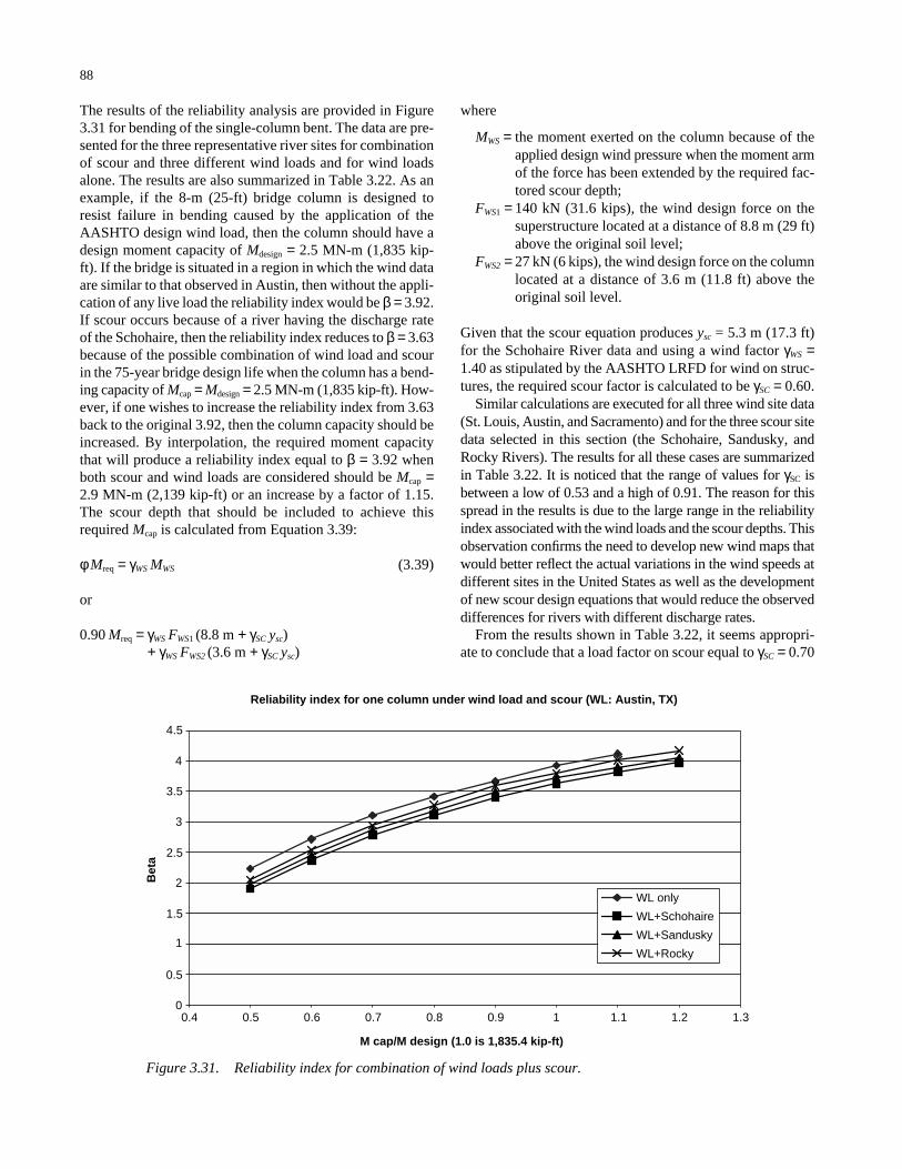
The results of the reliability analysis are provided in Figure3.31 for bending of the single-column bent. The data are pre-sented for the three representative river sites for combinationof scour and three different wind loads and for wind loadsalone. The results are also summarized in Table 3.22. As anexample, if the 8-m (25-ft) bridge column is designed toresist failure in bending caused by the application of theAASHTO design wind load, then the column should have adesign moment capacity of Mdesign = 2.5 MN-m (1,835 kip-ft). If the bridge is situated in a region in which the wind dataare similar to that observed in Austin, then without the appli-cation of any live load the reliability index would be β = 3.92.If scour occurs because of a river having the discharge rateof the Schohaire, then the reliability index reduces to β = 3.63because of the possible combination of wind load and scourin the 75-year bridge design life when the column has a bend-ing capacity of Mcap = Mdesign = 2.5 MN-m (1,835 kip-ft). How-ever, if one wishes to increase the reliability index from 3.63back to the original 3.92, then the column capacity should beincreased. By interpolation, the required moment capacitythat will produce a reliability index equal to β = 3.92 whenboth scour and wind loads are considered should be Mcap =2.9 MN-m (2,139 kip-ft) or an increase by a factor of 1.15.The scour depth that should be included to achieve thisrequired Mcap is calculated from Equation 3.39:

φMreq = γWS MWS (3.39)

or

0.90 Mreq = γWS FWS1 (8.8 m + γSC ysc) + γWS FWS2 (3.6 m + γSC ysc)

88

where

MWS = the moment exerted on the column because of theapplied design wind pressure when the moment armof the force has been extended by the required fac-tored scour depth;

FWS1 = 140 kN (31.6 kips), the wind design force on thesuperstructure located at a distance of 8.8 m (29 ft)above the original soil level;

FWS2 = 27 kN (6 kips), the wind design force on the columnlocated at a distance of 3.6 m (11.8 ft) above theoriginal soil level.

Given that the scour equation produces ysc = 5.3 m (17.3 ft)for the Schohaire River data and using a wind factor γWS =1.40 as stipulated by the AASHTO LRFD for wind on struc-tures, the required scour factor is calculated to be γSC = 0.60.

Similar calculations are executed for all three wind site data(St. Louis, Austin, and Sacramento) and for the three scour sitedata selected in this section (the Schohaire, Sandusky, andRocky Rivers). The results for all these cases are summarizedin Table 3.22. It is noticed that the range of values for γSC isbetween a low of 0.53 and a high of 0.91. The reason for thisspread in the results is due to the large range in the reliabilityindex associated with the wind loads and the scour depths. Thisobservation confirms the need to develop new wind maps thatwould better reflect the actual variations in the wind speeds atdifferent sites in the United States as well as the developmentof new scour design equations that would reduce the observeddifferences for rivers with different discharge rates.

From the results shown in Table 3.22, it seems appropri-ate to conclude that a load factor on scour equal to γSC = 0.70

Figure 3.31. Reliability index for combination of wind loads plus scour.

Reliability index for one column under wind load and scour (WL: Austin, TX)

0

0.5

1

1.5

2

2.5

3

3.5

4

4.5

0.4 0.5 0.6 0.7 0.8 0.9 1.11 1.2 1.3

M cap/M design (1.0 is 1,835.4 kip-ft)

Bet

a

WL only

WL+Schohaire

WL+Sandusky

WL+Rocky

in combination with a wind load factor of γWS = 1.40 is appro-priate for use when studying the combination of scour andwind loads. This γSC = 0.70 value is lower than that used forcombining scour and live loads because there are fewer windstorms expected in the 75-year design life of a bridge struc-ture as compared with the number of truck loading events.Fewer load occurrences imply a lower chance for combininghigh wind load intensity with high scour depth.

3.3.5 Combination of Scour and VesselCollision (SC + CV)

The single-column bent described in Figure 3.1 is ana-lyzed to illustrate how the combined effects of scour and ves-sel collision forces will affect the bent’s reliability. Scour datafrom the Mississippi River at the location of the I-40 bridgeare used in combination with the barge traffic at that location.Appendix C provides the basic river discharge data for theselected site. In addition, vessel collision forces as assembledin Figure 2.13 are used. The reliability calculations followthe Ferry-Borges model described in Section 2.5. The fol-lowing assumptions are made:

• Scour depths last for 6 months, during which time theerosion of the soil around the column base remains at itshighest value. The scour depth remains constant through-out the 6-month period.

• The scour depths are independent from year to year.• The site is on the average exposed to one major scour in

1 year. • The probability distribution of the maximum yearly dis-

charge rate follows a lognormal distribution. This max-imum yearly discharge rate is assumed to control thescour depth for the year. It is noted that because Equa-tion 2.31 was developed based on data from small rivers,this model may not be valid for rivers with high dis-charge rates. For this reason, this analysis is based onthe model developed in Appendix B based on the dataprovided by Johnson and Dock (1998) as expressed in

89

Equation 2.30 with a scour modeling variable, λsc, hav-ing a mean value equal to 0.55 and a COV of 52%.

• The collision force data are assumed to follow the prob-ability distribution curve shown in Figure 2.13.

• Each site will be exposed to 0.83 barge flotilla collisionsin 1 year.

• Equation 2.11 is used to find the probability distributionof the wind load for a 6-month period for studying thereliability caused by the application of wind loads whenscour is on.

• The effect of the scour depth in increasing the momentarm of the collision force is combined with the effectsof the 6-month collision force and projected to providethe maximum expected combined load in the 75-yearbridge design life period using the Ferry-Borges modeldescribed in Section 2.5. The calculations account forthe cases in which the collision occurs with the 6-monthscour on and the cases in which the collision occurs whenno scour is on.

• The reliability calculations are executed for columnbending because overtipping is mostly balanced by theweight of the structure and is not significantly affectedby the presence of scour.

• The reliability calculations account for the uncertaintiesassociated with predicting the discharge rate, estimatingthe scour depth given a discharge rate, projecting thecollision force magnitude, estimating the counter effectcaused by the soil resistance, and estimating the momentcapacity of the column.

• Referring to Figure 3.4, the failure equation for bendingin the column may be represented as follows:

(3.40)

Z MDK f

F e y f

F e f

p

n nCV sc

nCV

= +

− ( ) + +

+[ ]

col cyc3

6

3

1

1

1 2

3

γλ

( )

maxmax max ( )

max ( )

*

**

TABLE 3.22 Summary of live load factors for combination of SC plus WS

Wind data Scour data Mreq FWS1 FWS2 ysc (ft) γSC for WS + SC

Austin Schohaire 2,139 (kip-ft) 31.6 (kips) 6 (kips) 17.3 0.60

Austin Sandusky 2,050 31.6 6 14.3 0.62

Austin Rocky 1,945 31.6 6 12.3 0.57

Sacramento Schohaire 2,314 31.6 6 17.3 0.77

Sacramento Sandusky 2,260 31.6 6 14.3 0.87

Sacramento Rocky 2,191 31.6 6 12.3 0.91

St. Louis Schohaire 2,072 31.6 6 17.3 0.53

St. Louis Sandusky 2,004 31.6 6 14.3 0.56

St. Louis Rocky 1,959 31.6 6 12.3 0.59

Average 0.67

where

Mcol = the bending moment capacity of the column, FCV* = the collision force on the structure that occurs

when scour is on, FCV** = the collision force on the structure when there

is no scour, γ = the specific weight of the soil,

D = the column diameter, Kp = the Rankine coefficient,

f = the distance below the soil level at whichthe maximum bending moment occurs,

λcyc = the factor that accounts for the effect of cyclicloads on foundation strength,

e1 = the eccentricity of the collision force rela-tive to the soil level (before scour),

ysc = the scour depth,n1 = the number of scours expected in a 75-year

period (n1 = 75), n2 = the number of collisions expected within 1

year when there is scour (n2 = 0.42), andn3 = the number of collisions that occur when

there is no scour (n3 = 0.42 ∗ 75).

The results of the reliability analysis are provided in Fig-ure 3.32 for bending of the single-column bent. The resultsshow that if the 150-ft bridge column is designed to resistfailure in bending caused by the application of the collisionforces determined using the AASHTO specifications and fol-lowing the model of Whitney et al. (1996), the column should

90

have a design moment capacity Mdesign = 464 MN-m (342,333kip-ft). The corresponding reliability index—assuming thatno scour is possible—would be β = 2.78. If the bridge isexposed to scour because of a river having the discharge rateof the Mississippi and the channel profile shown in Figure3.6, then the reliability index reduces to β = 2.05 because ofthe possible combination of collision forces and scour in the75-year bridge design life when the column capacity of Mcap =Mdesign = 464 MN-m (342,333 kip-ft). However, if we wish toincrease the reliability index from 2.05 back to the original2.78, then the column capacity should be increased. By inter-polation, the required moment capacity that will produce areliability index equal to β = 2.78 when both scour and ves-sel collisions are considered should be Mcap = 715 MN-m(527,200 kip-ft) or an increase by a factor of 1.54. To achievethis Mcap, the following design equation should be satisfied:

φMreq = γCV MCV (3.41)

or

where

MCV = the moment exerted on the column caused by theapplied design wind pressure when the moment arm

0 90 4 9

36

3

. ( . )M F m y f

DK f

CV CV SC SC

p

req = + +

−

γ γ

γ

Reliability index for moment capacity under ship collision and scour

0

0.5

1

1.5

2

2.5

3

3.5

4

4.5

0.4 0.6 0.8 1 1.2 1.4 1.6 1.8 2M cap/M design

(1.0 is 342,333 kip-ft)

Bet

a

collision only

collision+scour

Figure 3.32. Reliability index for combination of collision and scour.

of the force has been extended by the required fac-tored scour depth;

γ = the specific weight of the soil; D = the column diameter; Kp = the Rankine coefficient;

FCV = 35 MN (7,900 kips), the vessel collision design forceon the column applied at a distance of 16 ft abovethe original soil level; and

f = 10.5 m (34.5 ft) = the depth to the point of maxi-mum moment.

Note that in this equation the effect of the soil resistance isincluded because f is reasonably deep. For the cases analyzedabove (e.g., wind loads), f is relatively small and the contri-butions of the soil resistance does not significantly affect thedesign capacity of the column. Given that the scour equationproduces ysc = 10.4 m (34.2 ft) for the Mississippi River dataand using a vessel collision factor γCV = 1.0 as stipulated bythe AASHTO LRFD for collision forces, the required scourfactor is calculated to be γSC = 0.62.

From the calculations shown above, it seems appropriateto conclude that a load factor on scour equal to γSC = 0.60associated with γCV = 1.0 is reasonable for use when studyingthe combination of scour and ship collision forces. This valueis lower than that used for combining scour and live loadsand for combining wind and scour because there are fewercollisions expected in the 75-year design life of a bridge struc-ture as compared with the number of truck loading events orwindstorms. Fewer load occurrences imply a lower chancefor combining high vessel collision forces with high scourdepths. Also, the target reliability index selected for the cal-ibration is lower than that used for live loads and is lowerthan that obtained from the average of different wind data.The lower target reliability index is selected to match the reli-ability index observed for the cases in which vessel collisionsoccur without risk of scour.

3.3.6 Combination of Vessel Collision andWind Loads (CV + WS)

In this section, the single-column bent described in Figure3.1 is analyzed to illustrate how the combined effects of ves-sel collision forces and wind loads will affect its reliability.It is herein assumed that wind load data collected in Knox-ville, Tennessee, are applicable for this bridge site. This Knox-ville wind data are used in combination with the barge traf-fic at the location of the I-40 bridge in Memphis. In addition,vessel collision forces as assembled in Figure 2.13 are used.The reliability calculations follow the Ferry-Borges modeldescribed in Section 2.5. The following assumptions are made:

• The wind speed data are assumed to follow a Gumbeldistribution, with a yearly mean value equal to 77.8 km/h(48.6 mph) and COV of 14%.

• The site is exposed to 200 winds in 1 year.

91

• Equation 2.14 is used to find the probability distributionof the wind load for a 6-month period for studying thereliability caused by the application of wind loads whenscour is on.

• The collision force data are assumed to follow the prob-ability distribution curve shown in Figure 2.13.

• Each site will be exposed to an average of 0.83 bargeflotilla collisions in 1 year.

• Equation 2.14 is used to find the probability distributionof the wind load for a 6-month period for studying thereliability caused by the application of a collision forcewhen the wind is on.

• A correlation between the wind speed and the numberof collisions is assumed based on the data provided byLarsen (1993). According to this model, the rate ofcollisions increases by a factor of 3 (from 0.83 to 2.50collisions/year) when the wind speed increases from 6m/sec (13 mph) to 14 m/sec (31 mph). Below 6 m/sec(13 mph), the number of collisions remains at 0.83 col-lisions/year; beyond 14 m/sec (31 mph), the number ofcollision remains at a rate of 2.50/year. Although bargesand flotilla may not travel when the wind speeds exceedthe 14 m/sec (31 mph) limit, it is herein assumed thatvessels and barges may break from their moorings whenthere is a large windstorm such that collisions are stillpossible.

• The effect of the moment from wind forces is combinedwith the effects of the collision force and projected toprovide the maximum expected combined load in the75-year bridge design life period using the Ferry-Borgesmodel described in Section 2.5. The calculations accountfor the cases in which the collision occurs during a wind-storm and the cases in which the collision occurs whenno wind is on.

• The reliability calculations are executed for columnbending because overtipping is mostly balanced by theweight of the structure.

• The reliability calculations account for the uncertaintiesassociated with predicting the wind speed, estimating thewind forces, projecting the collision force magnitude,estimating the counter effect caused by the soil resistance,and estimating the moment capacity of the column.

• Referring to Figure 3.4, the failure equation for bendingin the column may be represented as follows:

(3.42)

where

Mcol = the bending moment capacity of the column,

Z MDK f

F e f F e f

F e f

p

nWS

nCV

nCV

= +

−+ + +

+

( )[ ][ ]

col cyc

3

6

3

2 2

2

1 2

3

γλ

( )

maxmax ( ) max ( )

max ( )

*

**

FCV* = the collision force on the structure that occurswhen a wind is on,

FCV** = the collision force on the structure when thereis no wind,

γ = the specific weight of the soil, D = the column diameter, Kp = the Rankine coefficient,

f = the distance below the soil level at which themaximum bending moment occurs,

λcyc = the factor that accounts for the effect of cyclicloads on foundation strength,

e2 = the eccentricity of the collision force rela-tive to the soil level,

e1 = the moment arm of the resultant wind force,n1 = the number of winds expected in a 75-year

period (n1 = 200 × 75),n2 = the number of collisions expected when there

is a wind, and n3 = the number of collisions that occur when

there is no wind.

In order to study the effects of the winds on the structure andcalculate the wind force, FWS, the results provided in Appen-dix F are used. The results essentially show that at a wind of70 mph the wind force is equal to 18.6 MN (4,180 kips) andthat the resultant force will be applied at an eccentricity e1 =68 m (223 ft) from the soil’s surface. Interpolation as a func-

92

tion of V 2 (where V = wind velocity) is used to find the windforces for different wind speeds. Notice that the force eccen-tricity is larger than the column height because of the effectof the superstructure.

The results of the reliability analysis are provided in Fig-ure 3.33 for bending of the single-column bent. For example,if the 46-m (150-ft) bridge column is designed to resist fail-ure in bending caused by the application of the collisionforces determined using the AASHTO specifications and fol-lowing the model of Whitney et al. (1996), then the columnshould have a design moment capacity of Mdesign = 464 MN-m(342,333 kip-ft). If the bridge was originally designed with-out taking into consideration the possibility of windstorms,the reliability index would be β = 2.78. If the bridge isexposed to winds in addition to collision forces, then the reli-ability index reduces to β = 0.82 in the 75-year bridge designlife when the column has a capacity Mcap = Mdesign = 464MN-m (342,333 kip-ft). However, if one wishes to increasethe reliability index from 0.82 back to the original 2.78, thenthe column capacity should be increased. By interpolation,the required moment capacity that will produce a reliabilityindex equal to β = 2.78 when both vessel collision forces andwind loads are considered should be Mcap = 896 MN-m(660,700 kip-ft) or an increase by a factor of 1.93. To achievethis Mcap, load combination factors should be used in thedesign equations. The determination of the appropriate loadfactors is executed using the following equation:

Figure 3.33. Reliability index for combination of vessel collision plus wind loads and scour.

Reliability index for ship collision under scour and wind load

-3

-2

-1

0

1

2

3

4

5

0.4 0.6 0.8 1.21.0 1.61.4 1.8 2.22 2.4

M cap/M design (1.0 is 342,333 kip-ft)

Bet

a

collision onlycollision+scourcollision+scour+windcollision+wind

φMreq = γWS MWS + γCV MCV (3.43)

or

0.90 Mreq = γWS 18.6 MN ∗ (68 m + 2 f /3) + γCV 35 MN ∗ (4.9 m + 2 f /3).

By trial and error, it has been determined that a γWS = 0.27associated with γCV = 1.0 would lead to a point of maximummoment located at a distance of f = 11.3 m (37 ft) below thesoil level. These factors will produce a required momentcapacity Mreq = 896 MN-m (660,700 kip-ft), which will leadto a reliability index of β = 2.78 for the combination of windloads and vessel collisions. The β = 2.78 is the same relia-bility index obtained from vessel collision forces alone.

In addition to showing how the reliability index variesfor the cases in which vessel collision forces are appliedalone on the bridge, Figure 3.33 shows how the combina-tion of wind forces, collision forces, and scour affect thereliability index. It is noted that the probability of having allthree extreme events simultaneously is very small. Hence,the drop in the reliability index from the case in which windand vessel collision forces are combined to the case inwhich wind, scour, and vessel collision are combined is lessthan 0.1. Therefore, it is not necessary to check this possi-ble combination. Based on the calculations performed inthis section it is recommended to use a wind load factor ofγWS = 0.30 in combination with γCV = 1.0 when checking thesafety of bridges under the combined effects of winds andvessel collisions. The 0.30 wind factor proposed is lowerthan the 0.80 factor used for combinations involving liveloads. This is justified based on the lower number of vesselcollisions expected when compared with the number of liveload events, meaning there is a lower chance of combinationeven though a correlation between the rate of collisions ismade with the intensity of the wind while a negative corre-lation is made with the number of live load events with windspeeds. In addition, the target reliability index selected forwind plus vessel collision is lower than that used for liveloads with winds.

3.3.7 Combination of Earthquakes and Scour(EQ + SC)

In this section, the single-column bent described in Fig-ure 3.1 is analyzed to illustrate how the combined effects ofearthquakes and scour will affect its reliability. The datafrom the five earthquake sites with probability distributioncurves described in Figure 2.4 are used. The scour data areobtained from the USGS website for the Schohaire, San-dusky, and Rocky Rivers, as described in Section 2.4.4 (Table2.8). The reliability calculations follow the Ferry-Borgesmodel described in Section 2.5. The following assumptionsare made:

93

• Scour depths last for 6 months, during which time theerosion of the soil around the column base remains at itshighest value. The scour depth remains constant through-out the 6-month period.

• Scour depths are independent from year to year.• Each site is on the average exposed to one major scour

in 1 year. • The probability distribution of the maximum yearly dis-

charge rate follows a lognormal distribution. This max-imum yearly discharge rate is assumed to control thescour depth for the year.

• The intensity of the earthquake response is as shown inFigure 2.15.

• The number of earthquakes expected in 1 year is 8 for theSan Francisco site data, 2 for Seattle, 0.50 for Memphis,0.40 for New York, and 0.01 for St. Paul. This meansthat there will be 600 earthquakes in a 75-year returnperiod for San Francisco, 150 earthquakes for Seattle, 38in Memphis, 30 in New York, and 1 in St. Paul.

• The probability distribution of the maximum yearlyearthquake may be used to find the probability distribu-tion for a single event using Equation 2.14.

• Equation 2.14 is used to find the probability distributionof the earthquake intensities for different return periods.In particular, the earthquake intensity for t = 1/2-yearperiod is calculated for combination with the earthquakeload effects when the foundation is scoured.

• The effects of each scour are combined with the effectsof the 1/2-year earthquake intensity and projected to pro-vide the maximum expected combined load in the 75-year bridge design life period using the Ferry-Borgesmodel described in Section 2.5. The calculations accountfor the cases in which the earthquake occurs with the 1/2-year scour period and the cases in which an earthquakeoccurs when there is no scour.

• The reliability calculations are executed for the columnovertipping limit state. The column bending limit statewas not considered because the results of Figure 3.18show that the foundation depth does not significantlyaffect the reliability index for column bending. Thus,when a large length of the column is exposed because ofscour, the reduced column stiffness that ensues will resultin lower bending moment on the column base, and thereliability index remains practically unchanged. On theother hand, for column overtipping, the remaining soildepth may sometimes not be sufficient to resist overtip-ping even though the forces are reduced.

• The reliability calculations account for the uncertaintiesassociated with predicting the EQ intensity, estimatingthe bridge response given an EQ intensity, projectingthe scour depth, and estimating the soil capacity to resistovertipping.

• The failure equation for bending of the column underthe combined effect may be represented as follows:

(3.44)

where

γ = the specific weight of the soil; D = the column diameter; Kp = the Rankine coefficient; L = the foundation depth before scour; e = the distance from the original soil level to

the point of application of the inertial force;FEQ

* = the inertial force when the scour is on;FEQ

** = the inertial force when no scour is on;n1 = the number of scours expected in a 75-year

period (75 scours); n2 = the number of earthquakes expected in a

1/2-year period when scour is on; and n3 = the number of earthquake events expected in a

period equal to 75 years minus the times whena scour is on (i.e., n3 is the number of earth-quakes in a period equal to 37.5 years [75/2]).

The results of the reliability analysis are provided in Fig-ure 3.34 for the San Francisco earthquake data for differentvalues of foundation depth. The results that were obtained byconsidering the reliability of the bridge structure when onlyearthquakes are considered (i.e., by totally ignoring the effects

Z

DK L yF e L

DK LF e L

n

p

nEQ

n

p

EQ

=

−− +

− +

[ ]

max

max( )

max ( )

max( )

( )

*

**

1 2

3

3

6

3

6

3

3

γ

γ

scour

94

of scour) are also illustrated in Figure 3.34. The results forthe San Francisco site are summarized as shown in Table3.23. For example, if the bridge column is designed to satisfythe proposed revised AASHTO LRFD specifications (the seis-mic provisions) developed under NCHRP Project 12-49 (ATCand MCEER, 2002), then the required foundation depth for thecolumn using a 2,500-year earthquake return period is L =Ldesign = 26.06 m (85.5 ft). This would produce a reliabilityindex for overtipping (for a 75-year bridge design life) equalto β = 2.26 for sites having earthquake intensities similar tothose observed in San Francisco but that are not subject toscour. If one considers that the foundation may be weakenedby the presence of scour that would occur because of the riverhaving the discharge rate of the Schohaire, then the reliabilityindex for the column with a foundation depth of L = 26.06 m(85.5 ft) reduces to β = 2.24. If one wishes to increase thereliability index from 2.24 back to the original 2.26, then thedepth of the foundation should be increased. By interpola-tion, the required foundation depth that will produce a relia-bility index equal to β = 2.26, when both earthquake loadsand scour are considered, should be L = 26.33 m (86.4 ft) oran increase of 0.27 m (0.9 ft).

The Ldesign value 26.06 m (85.5 ft) includes the effect of theresistance factor for a lateral soil capacity of φ = 0.50. Thescour factor that should be used for the combination of earth-quakes and scour should be determined such that

(3.45)0 503

6

3

. ( )γ

γ γDK L

F e y LpEQ EQ SC SC

′ = + + ′

Reliability index for overtipping of one column under EQ and scour (San Francisco)

-1.5

-1

-0.5

0

0.5

1

1.5

2

2.5

3

0.2 .0.4 0.6 0.8 1.21

L actual/L design (1.0 is 85.5 ft)

Bet

a

EQ only

EQ+Schohaire

EQ+Sandusky

EQ+Rocky

Figure 3.34. Reliability index for earthquakes and scour for overtipping (San Francisco).

where

0.50 = the soil resistance factor; γ = the specific weight of the soil;

D = the column diameter; Kp = the Rankine coefficient; L ′ = the foundation depth after scour (L ′ = Lrequired −

γSC ySC); e = the distance from the original soil level to the point

of application of the inertial force; γEQ = the load factor for earthquake forces; FEQ = the inertial force; ysc = the design scour depth as shown in Table 3.4, which

for the Schohaire River is 5.3 m (17.3 ft); and γSC = the scour factor that should be used when consid-

ering the combination of earthquakes and scour.

It is noted that the inertial force, FEQ, is a function of L ′ andthe product γSC ySC. Hence the scour factor can only be foundfrom Equation 3.45 by trial and error.

The calibration of the load combination factor involves thedetermination of the values of γSC needed to produce therequired foundation depth Lreq = 26.3 m (86.4 ft). If the valuefor γEQ is preset at 1.0, then γSC is calculated to be equal to0.36. This would lead to a foundation L ′ after scour erosionequal to 24.2 m (79.3 ft). Notice that the L ′ = 24.2 m (79.3ft) is lower than the original L = 26.1 m (85.5 ft). This reduc-tion in the required effective foundation depth is due to theadditional flexibility of the column caused by the presence ofscour. In fact, when scour occurs, the clear height of the col-umn increases and the remaining foundation depth decreases;as long as the foundation is not totally washed out, this phe-nomenon would reduce the stiffness of the system and wouldlead to a higher natural period. When the natural periodincreases, the inertial forces decrease. Although the moment

95

arm of the force increases, the required foundation depth afterscour would be lower than originally required if no scour wereconsidered. It is noted however that adding 24.2 m (79.3 ft)plus 0.36 times the design scour depth (5.3 m = 17.3 ft)would still lead to a total foundation depth = 26.3 m (86.4 ft),which is higher than the original no scour depth L = 26.1 m(85.5 ft). It is also noted that in the examples solved in thissection, the mass of the system is not altered because of thepresence of scour or changes in foundation depth.

Similar calculations are executed for five earthquake sitesand three discharge data. Namely, the earthquake data usedcorrespond to those data from San Francisco, Seattle, Mem-phis, New York, and St. Paul. The scour data used correspondto those data from the Schohaire, Sandusky, and Rocky Rivers.The results from all 15 cases considered are summarized inTable 3.23. Notice that for all the cases considered, the scourfactor remains below 0.55, with an average value of 0.25.Based on the results shown in Table 3.23, it would seemappropriate to recommend that a scour factor of γSC = 0.25associated with an earthquake factor of γEQ = 1.00 be used toaccount for the combination of scour and earthquakes. The0.25 scour factor is lower than that observed for the combi-nation of scour and vessel collisions because the target reli-ability level used for the combination of scour and earth-quakes is lower than that used for collisions and scour (e.g.,for San Francisco, βtarget = 2.26 versus βtarget = 2.78 for vesselcollisions). Another reason is because the earthquake analy-sis model accounts for the additional flexibility of the systemwhen scour occurs and for the reduction in inertial force thatthis causes. The flexibility of the column is not directly con-sidered when analyzing the effect of vessel collision forces.

All the analyses for combinations involving scour assumethat scour lasts for a period of 6 months, during which timethe scour remains at its highest value. Because no models are

Earthquake site

Scour data

β target

Original foundation depth (ft)

Required foundation depth (ft)

Scour depth (ft)

γsc

Schohaire 86.42 17.34 0.36 Sandusky 86.19 14.33 0.36

San Francisco Rocky 2.259 85.5 85.99 12.32 0.34 Schohaire 67.04 17.34 0.18 Sandusky 66.80 14.33 0.17

Seattle Rocky 2.635 66 66.46 12.32 0.12 Schohaire 28.64 17.34 0.55 Sandusky 23.97 14.33 0.32

St. Paul Rocky 2.368 20 22.08 12.32 0.20 Schohaire 41.06 17.34 0.32 Sandusky 39.39 14.33 0.23

New York Rocky 2.491 37 38.55 12.32 0.18 Schohaire 60.00 17.34 0.18 Sandusky 59.59 14.33 0.16

Memphis Rocky 2.488 58.6 59.20 12.32 0.12 Average 0.25

TABLE 3.23 Summary of live load factors for combination of EQ plus SC

currently available to study the duration of live bed scours atbridge piers and how long it would take for the foundation ofdrilled shafts to regain their original strengths, a sensitivityanalysis is performed to study the effect of scour duration onthe results of the reliability analysis and the proposed loadfactor if the duration of scour is changed from 6 months toeither 4 or 8 months. The results are provided in Table 3.24,which shows a change in the load factor on the order of 0.05for each 2-month change in the scour duration. It is noted thatin all cases considered, the scour is assumed to be at its high-est value, which does provide a conservative envelope to thescour combination cases.

3.4 SUMMARY AND RECOMMENDATIONS

In this chapter, a reliability analysis of bridge bents is per-formed when the bridges are subjected to effects of live loads,wind loads, scour, earthquakes, vessel collisions, and com-binations of these extreme events. Load combination factorsare proposed such that bridges subjected to a combination ofthese events would provide reliability levels similar to thoseof bridges with the same configurations but situated in sitesin which one threat is dominant. Thus, the proposed load fac-tors are based on previous experiences with “safe bridge struc-tures” and provide balanced levels of safety for each loadcombination. The results of this study found that differentthreats produced different reliability levels. Therefore, thetarget reliability indexes for the combination of events areselected in most cases to provide the same reliability levelassociated with the occurrence of the individual threat withthe highest reliability index. Thus, when dealing with the com-bination of live load plus wind load or live load plus scour,

96

the reliability index associated with live loads is used as tar-get. When studying the reliability of bridges subjected to thecombination of wind loads and scour, the reliability indexassociated with wind loads alone is chosen for target. Simi-larly, when studying the reliability of bridges subjected to ves-sel collisions with scour or vessel collision with wind load, thereliability index associated with vessel collisions is used fortarget. For combinations involving earthquake loads, it is thereliability index associated with earthquakes alone that is usedfor target. Combinations involving earthquakes are treated dif-ferently than are other combinations because of the large addi-tional capacity that would be required to increase the reliabil-ity levels of bridges subjected to earthquake risks. Thisapproach is consistent with current earthquake engineeringpractice, which has determined that current earthquake designmethods provide sufficient levels of safety given the costs thatwould be involved if higher safety levels were to be specified.

Results of the reliability analyses indicate that there arelarge discrepancies among the reliability levels implied in cur-rent design practices for the different extreme events underconsideration. For example, the AASHTO LRFD was cali-brated to satisfy a target member reliability index equal to 3.5for gravity loads. The calculations performed in this study con-firm that bridge column bents provide reliability index valuesclose to the target 3.5 for the different limit states considered.These limit states include column bending, axial failure, bear-ing failure of the soil for one-column and multicolumn bents,and overtipping of one-column bents. The reliability indexvalues calculated for each of these limit states show that βranges from about 2.50 to 3.70. The lowest value is for foun-dation failures in bearing capacity. This is due to the largelevel of uncertainty associated with determining the strengthsof foundation systems. The highest value is for bending

TABLE 3.24 Sensitivity of results to scour duration period

Earthquake site

Scour data

Required foundation depth (ft)

(4 months)

Required foundation depth (ft)

(6 months)

Required foundation depth (ft)

(8 months)

γ sc (4 months)

γ sc (6 months)

γ sc (8 months)

Schohaire 86.15 86.42 86.43 0.29 0.36 0.36

Sandusky 86.01 86.19 86.38 0.30 0.36 0.42 San Francisco Rocky 85.87 85.99 86.07 0.29 0.34 0.38

Schohaire 66.84 67.04 67.56 0.15 0.18 0.25

Sandusky 66.68 66.80 67.24 0.15 0.17 0.25 Seattle Rocky 66.16 66.46 66.75 0.04 0.12 0.19

Schohaire 28.58 28.64 28.68 0.55 0.55 0.56

Sandusky 23.76 23.97 24.28 0.30 0.32 0.34 St. Paul Rocky 21.52 22.08 22.40 0.15 0.20 0.23

Schohaire 40.15 41.06 41.52 0.25 0.32 0.35

Sandusky 38.67 39.39 39.81 0.17 0.23 0.27 New York Rocky 38.11 38.55 38.98 0.13 0.18 0.23

Schohaire 59.85 60.00 60.57 0.16 0.18 0.25

Sandusky 59.49 59.59 60.12 0.15 0.16 0.24 Memphis Rocky 59.12 59.20 59.58 0.11 0.12 0.19

Average 0.21 0.25 0.30

moment capacity. These reliability indexes are for memberfailures. If there is sufficient redundancy, the system reliabil-ity is higher as explained by Ghosn and Moses (1998) and Liuet al. (2001).

The system reliability index for bridge bents subjected toearthquakes is found to be on the order of 2.80 to 3.00 forthe moment capacity of drilled shafts supporting single- andmulticolumn bents or 2.20 to 2.60 for overtipping of single-column bents. These values are for bridges designed fol-lowing the proposed specifications developed under NCHRPProject 12-49 (ATC and MCEER, 2002]. These reliabilitylevels decrease to as low as 1.75 when studying the safety ofbridge columns under earthquakes. The large difference isdue to the differences in the response modification factorsrecommended for use during the design process. In fact,NCHRP Report 472 recommends the use of different responsemodification factors for bridge subsystems depending on theconsequences of failure (ATC and MCEER, 2002). Unlikethe analysis for other hazards, the earthquake analysis pro-cedure accounts for system capacity rather than for membercapacity because failure is defined by accounting for plasticredistribution of loads and the ductility capacity of the col-umns. Although relatively low compared with the memberreliability index for gravity loads, the engineering commu-nity is generally satisfied with the current safety levels asso-ciated with current earthquake design procedures. For this rea-son, the target reliability index for load combination casesinvolving earthquakes is chosen to be the same reliabilityindex calculated for the case in which earthquakes alone areapplied. In fact, the results of this study indicate that verylittle improvement in the earthquake reliability index can beachieved even if large increases in the load factor are imple-mented. This is because much of the uncertainties in assessingthe earthquake risk for bridge systems are due to the difficultyin predicting the earthquake intensities over the design lifeof the bridge. Improvement in the overall earthquake designprocess can only be achieved after major improvements in theseismologists’ ability to predict future earthquakes.

The reliability index for designing bridge piers for scourfor small-size rivers is on the order of 0.45 to 1.7, which ismuch lower than the 3.5 target for gravity loads and evenlower than the range observed for earthquakes. In addition,failures caused by scour generally result in total collapse ascompared with failures of members under gravity loads.This observation is consistent with the observation made byShirole and Holt (1991) that, by far, most U.S. bridge col-lapses are due to scour. Because of the high risks of major col-lapses caused by scour, it is recommended to increase the reli-ability index for scour by applying a scour safety factor equalto 2.00. The application of the recommended 2.00 safety fac-tor means that if current HEC-18 scour design procedures arefollowed, the final depth of the foundation should be 2.00times the value calculated using the HEC-18 approach. Sucha safety factor would increase the reliability index for scourfrom an average of about 1.00 to slightly more than 3.0, which

97

will make the scour design methods produce average safetylevels for small rivers more compatible with the methods forother threats. However, the wide range in safety levels willrequire a review of current scour evaluation procedures.

Current AASHTO LRFD bridge design methods for windloads provide average member reliability index values closeto 3.00. However, there are large differences between thereliability indexes obtained for different U.S. sites. In fact,for the sites analyzed in this report, the reliability index (β)ranges between 2.40 and 4.00. The wind design approach isbased on member safety. If sufficient levels of redundancyexist, the system reliability would be higher. The system reli-ability could increase by 0.25 to 0.50 over member reliabil-ity, depending on the number of columns in the bridge bentand the level of confinement of the columns. However, thelarge variations observed in the reliability index indicate thatthere should be major research effort placed on improvingthe current wind design procedures. This effort should bedirected toward better understanding the behavior of bridgessubjected to wind loads and toward developing new winddesign maps that would provide more uniform safety levelsfor different regions of the United States.

The AASHTO vessel collision model produces a reliabil-ity index of about 3.15 for shearing failures and about 2.80for bending failures. The higher reliability index for shear isdue to the implicit biases and conservatism associated withthe AASHTO LRFD shear design procedures as reported byNowak (1999). The presence of system redundancy causedby the additional bending moment resistance by the bents,abutments, or both that are not impacted would increase thereliability index for bending failures to more than 3.00, mak-ing the safety levels more in line with those for shearing fail-ures and those of bridge members subjected to the other threatsconsidered.

The results of the reliability index calculations for indi-vidual threats are used to calibrate load combination factorsapplicable for the design of short- to medium-span bridges.The recommended load combination factors are summa-rized in Appendix A in a format that is implementable in theAASHTO LRFD specifications.

The load combination factors proposed in this study illus-trate that the current load factors for the combination of windplus gravity loads lead to lower reliability indexes than dothose of either load taken separately. Hence, this study hasrecommended increasing the load factors for wind on struc-tures and wind on live loads from the current 0.40 to 1.20 incombination with a live load factor of 1.00, which replacesthe live load factor of 1.35. If the 1.35 live load factor ismaintained, then the wind factor should be set equal to 0.80.

The commonly used live load factor equal to 0.50 in com-bination with earthquake effects leads to conservative results.This report has shown that a load factor of 0.25 on live loadeffects when they are combined with earthquake effectswould still provide adequate safety levels for typical bridgeconfigurations subjected to earthquake intensities similar to

those observed on the West or the East Coast. These calcu-lations are based on conservative assumptions on the recur-rence of live loads when earthquakes are actively vibratingthe bridge system.

For the combination of vessel collision forces and windloads, a wind load factor equal to 0.30 is recommended incombination with a vessel collision factor of 1.0. The lowwind load factor associated with vessel collisions comparedwith that recommended for the combination of wind loadsplus live loads partially reflects the lower rate of collisions inthe 75-year design life of bridges as compared with the num-ber of live load events.

A scour factor equal to 1.80 is recommended for use in com-bination with a live load factor equal to 1.75. The lower scourload factor for combination of scour and live loads as com-pared with the load factor proposed for scour alone reflects thelower probability of having the maximum possible 75-yearlive load occur when the scour erosion is also at its maximum75-year depth.

A scour factor equal to 0.70 is recommended in combina-tion with a wind load factor equal to 1.40. The lower scourfactor observed in combination involving wind loads as com-pared with those involving live loads reflect the lower num-ber of wind storms expected in the 75-year design life of thestructure.

A scour factor equal to 0.60 is recommended in combi-nation with vessel collision forces. The lower scour factorobserved in combinations that involve collisions reflectsthe lower number of collisions excepted in the 75-year bridgedesign life.

A scour factor equal to 0.25 is recommended in combina-tion with earthquakes. The lower scour factor with earth-quakes reflects the fact that as long as a total wash out of thefoundation does not occur, bridge columns subjected to scourexhibit lower flexibilities that will help reduce the inertialforces caused by earthquakes. This reduction in inertial forcespartially offsets the scour-induced reduction in soil depth andthe resulting soil resisting capacity.

With regard to the extreme loads of interest to this study,the recommended revisions to the AASHTO LRFD specifi-cations (1998) would address the extreme loads by ensuringthat the factored member resistances are greater than the max-imum load effects obtained from the following combinations:

• Strength I Limit State: 1.25 DC + 1.75 LL• Strength III Limit State: 1.25 DC + 1.40 WS• Strength V Limit State: 1.25 DC + 1.00 LL

+ 1.20 WS + 1.20 WL• Extreme Event I: 1.25 DC + 0.25 LL

+ 1.00 EQ• Extreme Event II: 1.25 DC + 0.25 LL

+ 1.00 CV, or1.25 DC + 0.30 WS+ 1.00 CV (3.46)

98

• Extreme Event III: 1.25 DC; 2.00 SC, or 1.25 DC + 1.75 LL; 1.80 SC

• Extreme Event IV: 1.25 DC + 1.40 WS; 0.70 SC

• Extreme Event V: 1.25 DC + 1.00 CV; 0.60 SC

• Extreme Event VI: 1.25 DC + 1.00 EQ; 0.25 SC

In the above equations, DC represents the dead load effect,LL is the live load effect, WS is the wind load effect on thestructure, WL is the wind load acting on the live load, EQ isthe earthquake forces, CV is the vessel collision load, and SCrepresents the design scour depth. The dead load factor of1.25 would be changed to 0.9 if the dead load counteracts theeffects of the other loads.

Notice that no calculations for the combination of vesselcollisions and live loads are performed in this study becauseno live load models are currently available to cover the long-span bridges most susceptible to this combination. The γLL =0.25 factor proposed under Extreme Event II is projected fromthe calibration for the combination of earthquakes and liveloads under Extreme Event I.

Unlike the other extreme events, scour does not produce aload effect. Scour changes the geometry of the system andreduces the load-carrying capacity of the foundation in such away as to increase the risks from other failures. The presenceof scour is represented in the above set of Equations 3.46through the variable SC. The semicolon indicates that theanalysis for load effects should assume that a maximum scourdepth equal to γSC SC exists when the load effects of the otherextreme events are applied where gSC is the scour factor bywhich scour depths calculated from the current HEC-18method should be multiplied. When scour is possible, thebridge foundation should always be checked to ensure that thefoundation depth exceeds 2.00 SC. For the cases involving adynamic analysis, such as the analysis for earthquakes, it is verycritical that the case of zero scour depth be checked because inmany cases, the presence of scour may reduce the applied iner-tial forces. The resistance factors depend on the limit statesbeing considered. When a linear elastic analysis of single andmulticolumn bents is used, the system factors developed underNCHRP Project 12-47 should also be applied (Liu et al., 2001).

Equation 3.46 does not include any combinations of threedifferent threats. This is because several analyses executed aspart of this study have shown that the reductions of the reli-ability indexes for the combination of three different extremeevents are small. This is due to the low probability of a simul-taneous occurrence of three extreme events with high enoughintensities to affect the overall risk. This is illustrated in Fig-ure 3.33 for the combination of ship collisions with scour andwinds loads and in Figure 3.35 for the combination of liveload, wind, and scour.

99

Reliability index for overtipping of one column under live load, wind load, and scour

-2

-1

0

1

2

3

4

5

0.4 0.9 1.4 1.9 2.4

L actual/L design(1.0 is 6 ft)

Bet

a

LL only

LL+ Schohaire

LL+WL+ Schohaire

Figure 3.35. Reliability index for combination of live load, wind, and scour.

100

CHAPTER 4

CONCLUSIONS AND FUTURE RESEARCH

4.1 CONCLUSIONS

This study has developed a design procedure for the appli-cation of extreme load events and the combination of their loadeffects in the AASHTO LRFD Bridge Design Specifications(1998). This is achieved by proposing a set of load factors cal-ibrated using a reliability-based procedure that is consistentwith the reliability methodology of the AASHTO LRFD spec-ifications. The load events considered in this study includelive loads, earthquakes, wind loads, ship collision loads, andscour. The reliability analysis of the effects of each loadtaken individually is performed using methods developed inprevious bridge code calibration efforts (for the live loadsand ship collisions) and during the development of other struc-tural codes (for wind loads and earthquake loads). Because thecurrent specifications for scour were not based on reliabilitymethods, a scour reliability model has been developed for thepurposes of this study. In addition, the Ferry-Borges modelis used to evaluate the reliability of bridges under the com-bined effects of extreme load events. Results from the relia-bility of typical bridge configurations under the effects ofindividual threats are used to define target reliability levelsfor the development of load factors applicable for designingbridges that may be susceptible to a combination of threats.The objective is to recommend a rational and consistent setof load combination factors that can be implemented in futureversions of the AASHTO LRFD specifications.

To achieve the objectives of the study, this project firstreviewed the basic reliability methodology used during pre-vious code calibration efforts. Basic bridge configurationsdesigned to satisfy the current AASHTO specifications wereanalyzed to find the implicit reliability index values for dif-ferent limit states for bridges subjected to live loads, windloads, earthquakes, vessel collisions, or scour. The limit statesconsidered include column bending, shearing failure, and axialfailure of bridge columns, bearing failure of column founda-tions, and overtipping of single-column bents. The reliabilityanalysis used appropriate statistical data on load occurrencesand load intensities for the pertinent extreme events that wereassembled from the literature and USGS websites. Statisticaldata on member and foundation capacities as well as loadanalysis models commonly used in reliability-based code cal-ibration efforts were also used to find the probability of fail-ure and the reliability index values for each extreme event.

Reliability indexes were calculated for the same bridges whensubjected to the combination of extreme events using theFerry-Borges model. The results were subsequently used tocalibrate load combination factors appropriate for implemen-tation in the LRFD equations.

The load factors are proposed such that bridges subjectedto a combination of events provide reliability levels similarto those of bridges with the same configurations but situatedat sites where one threat is dominant. Thus, the proposed loadfactors are based on previous experiences with “safe bridgestructures” and provide balanced levels of safety for each loadcombination. Because this study found that different threatsproduced different reliability levels, the target reliabilityindexes for the combination of events are selected in mostcases to provide the same reliability level associated with theoccurrence of the individual threat with the highest reliabil-ity index. Thus, when dealing with the combination of liveload plus wind load or live load plus scour, the reliability indexassociated with live loads is used as target. When studying thereliability of bridges subjected to the combination of windloads and scour, the reliability index associated with windloads alone is chosen for target. Similarly, when studying thereliability of bridges under vessel collision with scour or ves-sel collision with wind load, the reliability index associatedwith vessel collisions is used for target. For combinationsinvolving earthquake loads, it is the reliability index associ-ated with earthquakes alone that is used for target. Combina-tions involving earthquakes are treated differently than othercombinations because of the large additional capacity thatwould be required to increase the reliability levels of bridgessubjected earthquake risks.

The analysis considered structural safety as well as foun-dation safety. For two-column bents, system safety is com-pared with member safety. The results show that the systemproduces an additional reliability index about 0.25 higherthan the reliability index of the individual members, which isconsistent with the results of Liu et al. (2001) for drilled shaftsof two-column bents formed by unconfined concrete columns.Hence, the system factors calibrated by Liu et al. (2001) areapplicable for the cases in which linear elastic analysis is per-formed to check bridge member safety. Liu et al. (2001) cal-ibrated system factors for application on the left-hand side ofthe design equation to complement the member resistancefactor. The cases for which the application of system factors

101

is possible include the analysis of bridges subjected to com-binations exclusively involving live loads, wind loads, andship collision forces. The analysis for combinations involv-ing earthquakes is based on the plastic behavior of bridgebents; thus, system safety is directly considered and no sys-tem factors need to be applied. Scour causes the completeloss of the load-carrying capacity of a column, and bridgebents subjected to scour erosion exposing the full foundationwill have little redundancy. Thus, such failures should beassociated with system factors on the order of 0.80 as rec-ommended by Liu et al. (2001).

Results of the reliability analyses indicate that there arelarge discrepancies among the reliability levels implied incurrent design practices for the different extreme eventsunder consideration. Specifically, the following observationsare made:

• The AASHTO LRFD was calibrated to satisfy a targetmember reliability index equal to 3.5 for gravity loads.The calculations performed herein confirm that mem-bers provide reliability index values close to the target3.5 for the different limit states considered. These limitstates include column bending, axial failure and over-tipping of one-column bents. Lower reliability indexvalues are observed for foundation-bearing capacitiesfor one-column and multicolumn bents.

• The system reliability index for the drilled shaft founda-tions of bridge bents subjected to earthquakes is found tobe on the order of 2.9 for moment capacity or 2.4 forovertipping of single-column bents. Even lower reliabil-ity values are observed for bridge columns because ofthe higher response modification factor recommended forcolumn design as compared with those recommended forfoundation subsystems. Unlike the analysis for otherhazards, the earthquake analysis procedure accounts forsystem capacity rather than for member capacity. Thisis because earthquake analysis procedures consider theplastic redistribution of loads, and failure is defined basedon the ductility capacity of the members. Although rel-atively low compared with the member reliability indexfor gravity loads, the engineering community is gener-ally satisfied with the safety levels associated with cur-rent earthquake design procedures as improvements inthe reliability index would entail high economic costs.

• The reliability index for designing bridge piers set insmall rivers for scour varies from about 0.47 to 1.66,which is much lower than the 3.5 target for gravityloads. In addition, failures caused by scour result in totalcollapse as compared with failures of members undergravity loads that cause local damage only. Local dam-age can be sustained by the system if sufficient levels ofredundancy and ductility are present, which is not thecase for foundations exposed because of scour. Hence,it is recommended to increase the reliability index forscour by applying a scour safety factor equal to 2.00.

The application of the recommended 2.00 safety factormeans that if current HEC-18 scour design procedures arefollowed, the final depth of the foundation should be 2.00times the value calculated using the HEC-18 approach.Such a safety factor will increase the reliability index forscour from an average of about 1.0 to higher than 3.0.This increase will make the scour design methods morecompatible with the methods for other threats.

• Although bridge design methods for wind loads providean average member reliability index close to 3.0, there arelarge differences among the reliability indexes obtainedfor different U.S. sites. For this reason, it is recommendedthat research be undertaken to revise the existing windmaps so that they provide more consistent designs fordifferent regions of the United States.

• The AASHTO vessel collision model produces a relia-bility index of about 3.15 for shearing failures and on theorder of 2.80 for bending failures. The higher reliabilityindex for shear is due to the higher implicit biases andconservative design methods. The presence of systemredundancy caused by the reserve resistance provided bythe bents, abutments, or both that are not impacted wouldincrease the reliability index for bending failures to morethan 3.00, making the safety levels more in line withthose for shearing failures, which are brittle failures thatdo not benefit from the presence of redundancy.

The recommended load combination factors are summa-rized in Appendix A in a format that is implementable in theAASHTO LRFD specifications. The results illustrate the fol-lowing points:

• The current load factors for the combination of wind pluslive loads lead to lower reliability indexes than do thoseof either load taken separately. Hence, this study has rec-ommended increasing the load factors for wind on struc-tures and wind on live loads from the current 0.40 to 1.20in combination with a live load factor of 1.00.

• The commonly used live load factor equal to 0.50 incombination with earthquake effects would lead to con-servative results. This report has shown that a load fac-tor of 0.25 on live load effects when they are combinedwith earthquake effects would still provide adequatesafety levels for typical bridge configurations subjectedto earthquake intensities similar to those experienced onthe West and East Coasts. These calculations are basedon conservative assumptions on the recurrence of liveloads when earthquakes are actively vibrating the bridgesystem.

• For the combination of vessel collision forces and windloads, a wind load factor equal to 0.30 is recommendedin combination with a vessel collision factor of 1.0. Thelow wind load factor associated with vessel collisionscompared with that recommended for the combinationof wind loads plus live loads partially reflects the lower

102

rate of collisions in the 75-year design life of bridges ascompared with the number of live load events.

• For the combination of vessel collisions and live load, itis recommended to reduce the live load factor from 0.50to 0.25. This is proposed to bring this case more in linewith the earthquake plus live load case. A higher windload factor than live load factor is used in combinationsinvolving vessel collisions to reflect the fact that the rateof vessel collisions increases during windstorms.

• A scour factor equal to 1.80 is recommended for use incombination with a live load factor equal to 1.75. Thelower scour load factor for the combination of scour andlive loads compared with the factor recommended forscour alone reflects the lower probability of having themaximum possible 75-year live load occur when thescour erosion is also at its maximum 75-year depth.

• A scour factor equal to 0.70 is recommended in combi-nation with a wind load factor equal to 1.40. The lowerscour factor observed for the combination with windloads as compared with the combination with live loadsreflects the lower number of wind storms expected inthe 75-year design life of the structure.

• A scour factor equal to 0.60 is recommended in combi-nation with vessel collision forces. The lower scour fac-tor observed in combinations that involve collisionsreflects the lower number of collisions expected in the75-year bridge design life.

• A scour factor equal to 0.25 is recommended in combi-nation with earthquakes. The lower scour factor withearthquakes reflects the fact that as long as a total washout of the foundation does not occur, bridge columnssubjected to scour exhibit lower flexibilities that willhelp reduce the inertial forces caused by earthquakes.This reduction in inertial forces partially offsets thescour-induced reduction in soil depth and the resultingsoil resistance capacity.

• When scour is possible, the bridge foundation shouldalways be checked to ensure that the foundation depthexceeds 2.0 times the scour depth obtained from theHEC-18 equations.

• For the cases involving a dynamic analysis such as theanalysis for earthquakes, it is very critical that the case ofzero scour depth be checked because in many cases, thepresence of scour may reduce the applied inertial forces.

• When a linear elastic analysis of single-column andmulticolumn bents is used, the system factors developedunder NCHRP Project 12-47 should also be applied tocomplement the resistance factors (Liu et al., 2001).

4.2 FUTURE RESEARCH

The work performed as part of this study revealed that sev-eral issues related to the reliability analysis of bridge systemssubjected to extreme load events need further investigation.These issues include the following areas discussed below.

4.2.1 Evaluation of Proposed Load Factors

This report has recommended several changes in the loadfactors for extreme events and their combinations. These rec-ommendations are based on the reliability analysis of sim-plified models for typical bridge substructures subjected toindividual extreme events and the combination of events.Extensive field evaluation and experimentation with the pro-posed recommendations using detailed structural analysismodels should be undertaken. Some of these investigationsmay include extensive field measurements, data collection,and comparison of designs with evaluation of implied con-struction costs.

4.2.2 Determination of Appropriate TargetReliability Levels

The calibration of the load factors undertaken in thisresearch follows a commonly used approach whereby theaverage reliability index from typical “safe” designs is usedas the target reliability value for the new code. That is, a setof load factors and the nominal loads (or return periods for thedesign loads) are chosen for the new code such that bridgesdesigned with these factors will provide reliability index val-ues equal to the target value as closely as possible. Thisapproach that has traditionally been used in the calibration ofLRFD criteria (e.g., AISC and AASHTO) has led code writ-ers to choose different target reliabilities for different types ofstructural elements or for different types of loading condi-tions. The choice of the different target βs raises the followingquestion: If the reliability index (β) for live loads is 3.5 andfor earthquake loads is 2.8, what should be the target whencombining live loads and earthquake loads? In this report, itwas decided that the higher reliability index should be usedexcept for the cases involving earthquakes. The justificationis that increasing the reliability index for earthquake threatswould involve high construction costs, which society may notbe willing to sustain. This subjective justification for usingdifferent target reliabilities can be formulated using a risk-benefit argument. For example, codes should tolerate a higherrisk for the design of bridges (or structures) against a particu-lar event if the costs associated with reducing this risk areprohibitive. Aktas, Moses, and Ghosn (2001) have presentedexamples illustrating an approach that can be used for deter-mining the appropriate target reliability index values based onrisk-benefit analysis. More work is needed in that direction toimplement these concepts in actual bridge calibration efforts.

4.2.3 Reliability Models for Bridge Foundations

The analysis of bridge bents under the effect of the loadsconsidered in this study is highly dependent on the accuracyof the foundation analysis models and the uncertainties asso-ciated with predicting the strength capacity of bridge foun-dations. Similarly, the effects of the soil-structure interaction

103

on the response of bridge bents subjected to impact loading(i.e., vessel collisions) or cyclic dynamic loads (e.g., earth-quakes and winds) need to be carefully considered. Currently,there is little information available to describe the uncer-tainty inherent in commonly used foundation analysis proce-dures. These uncertainties are caused by modeling assump-tions, spatial variations of soil properties, and statisticaluncertainties due to the limitations in the soil samples that arenormally collected as part of the foundation design process.Some preliminary research work is currently ongoing underNCHRP Project 12-55. However, NCHRP Project 12-55 willnot address all the aspects of the problem—particularly thedynamic effects of the loads on soil strength—and moreresearch work is needed on this highly important subject.Reliability models should provide consistency between foun-dation analysis procedures and structural analysis models tobetter evaluate the reliability of complete structural systemsand the interaction among bridge superstructures, substruc-tures, and foundations.

4.2.4 Live Load Models

The statistical database used during the development ofthe live load model for the AASHTO LRFD code was col-lected from truck weight surveys in Ontario, Canada, andwas supplemented by limited samples from Michigan. Someof the limitations in the data include the following:

1. The Ontario truck weight data were collected in 1975 ina Canadian province that had higher truck weight lim-its than the ones currently in effect in the United States.

2. The Ontario data were biased toward heavy trucks (i.e.,only trucks that were believed to be heavily loaded wereweighed); this would obviously produce a weight his-togram showing an unusually high percentage of over-loaded vehicles.

3. The Michigan truck weight data were also biased becauseMichigan allows higher truck weight limits for certaintruck configurations than do most other U.S. states.

4. The statistics on multiple-truck occurrences used in thecalibration were not based on specific observations andwere unusually high compared with those observed ontypical highways.

5. The average daily truck traffic used in the calibrationwas low compared with that observed on typical high-ways.

6. The same live load factor and live load model were pro-posed for all bridges, although it is widely accepted thatbridges in rural areas with lower traffic counts are lesslikely to reach the projected maximum live load thanare bridges in heavily traveled industrial regions.

In general, these assumptions had to be made during the orig-inal calibration because of lack of sufficient data. It is herein

emphasized that, despite the limitations in the statistical data-base, the calibration process produces conservative estimatesof the reliability levels and robust sets of load factors. How-ever, the stated limitations in the database demonstrate thenecessity of collecting more data in order to obtain a betterassessment of the risks involved in current designs for var-ious types of bridges and also to provide a mechanism toinclude site-specific information. The load combination fac-tors depend on the number of live load events expected dur-ing the occurrence of the other loads. Hence, more informa-tion needs to be gathered on the rate and intensities of liveload events. Future live load models should be sufficientlyflexible to account for variations in these factors dependingon the sites considered, including the legal truck weight lim-its in effect at the site and the intensity of the traffic.

4.2.5 Wind Load Models

Considerable concern has been expressed regarding theconsistency of the data presented in the ASCE 7 maps thatare the basis for the AASHTO maps for wind speed intensi-ties. Some of the most pressing issues raised by researchersinclude the following:

1. Determining the proper probability distribution typethat most adequately represents the intensity of windspeeds for hurricanes and for regular storms;

2. Considering statistical uncertainty and the effect of thetails of the probability distributions;

3. Examining the relationship between the actually mea-sured wind speeds, including the regional variations ofwind intensities, and the adequacy of the wind speedenvelopes provided in the published maps;

4. Addressing the inconsistencies between the recurrenceintervals used in the maps for hurricane winds andwindstorms;

5. Remedying the lack of adequate models for represent-ing special cases such as tornados; and

6. Developing models to account for wind gusts on bridges.

It is clear that the effect of winds on civil engineering struc-tures in general and on bridge structures in particular did notreceive the same attention given to other loads, and morework is needed in this field in order to develop rational andconsistent design methods.

4.2.6 Scour Models

It is widely accepted that “a majority of bridges that havefailed in the United States and elsewhere have failed due toscour” (AASHTO, 1994). This is confirmed by Shirole andHolt (1991), who observed that over a 30-year period, morethan 1,000 of the 600,000 U.S. bridges have failed and that60% of these failures are because of scour while earthquakes

104

accounted for only 2%. Of course, there are many morebridges that are posted or otherwise taken out of service dueto their inadequate strengths (because of deterioration, lowrating, fatigue damage, etc.). Nevertheless, scour is consid-ered to be a critical cause of failure because its occurrenceoften leads to total collapse. For these reasons, developingmethods for the design and maintenance of bridge founda-tions for scour is currently considered to be a top priority foragencies concerned with the safety of bridges, and there isconsiderable research effort devoted to scour. The currentlyaccepted model for scour design and evaluation is the HEC-18 model. HEC-18 stipulates that the scour depth producedby a given flood is not affected by previous (or existing)scour at the site. Hence, the maximum scour in a given returnperiod is a function of the maximum flood observed in thatperiod and is not affected by previous smaller floods that mayhave occurred within that same period. In addition, the HEC-18 model assumes that the flood duration is always longenough for the full scour depth corresponding to the floodvelocity to be reached. Although, for live bed conditions, thescour hole is normally assumed to refill as the scour-causingflood recedes, the available literature does not provide pre-cise information on how long it normally takes for the foun-dation to regain its original strength. This is believed todepend on the type of material being deposited by live-bedstreams. It is also noted that HEC-18 was developed basedon small-scale experiments involving sandy materials. Scaleeffects and the effects of different soil types need to beaddressed in future research work. The importance of thescaling effect is reflected by the large differences observed inthe reliability levels of rivers based on their discharge ratesand expected scour depths. The differences between riverscour and tidal scour should also be addressed. Simultane-ously statistical data need to be gathered on each of the pa-rameters that affect scour in order to develop a comprehen-sive reliability model for scour that is compatible with themodels available for the other extreme events.

4.2.7 Vessel Collision Models

AASHTO’s Guide Specification and Commentary for Ves-sel Collision Design of Highway Bridges developed a detailed,reliability-based model for studying the safety of bridges sub-jected to vessel collision forces (AASHTO, 1991). The modelaccounts for the major parameters that affect the rate of colli-sions and the magnitude of the collision forces. However,more data are needed to verify several of the assumptions usedin the AASHTO model, including the effect of vessel size onthe geometric probability of collision, and to correlate the rateof accidents with site-specific information on the type andsize of the vessels, channel size and geometry, and other con-ditions. It is especially important to find explanations for thedifferences observed between the collision forces generatedin laboratory experiments or computer analyses and actualdamage observed after collisions in the field. These differ-

ences were lumped into a modeling random variable that wasidentified by the AASHTO guide specifications as the randomvariable x = Pactual /Pcalculated. Efforts should be made to reducethe discrepancies between the predicted and observed forcesto reasonable levels.

4.2.8 Earthquakes

Considerable effort has been expended over the last 3decades on developing rational and consistent models forstudying the safety of bridges subjected to earthquakes. Toprovide reasonable confidence levels, hazard maps and uni-form hazard response spectra have been developed for a finegrid covering the whole United States. The issues that stillrequire more research include the following:

1. Modeling of the ductility capacity and the relationshipbetween ductility capacity and response modificationfactors, particularly for multidegree-of-freedom sys-tems, taking into consideration the effects of theresponse modification factors on the overall reliabilityof bridge systems;

2. Development of SSI models that would provide con-sistent results for deep and shallow foundations;

3. Consideration of soil nonlinearity while determiningthe natural periods of the system;

4. Classification of soils for site amplification parametersand the consideration of uncertainties in determiningthe site factors.

4.2.9 Consideration of Modeling and Statistical Uncertainties

The research described in this report accounts for statisti-cal and modeling uncertainties by representing these throughrandom variables that are directly included in the calcula-tions of the reliability index, β. For example, during the cal-ibration of the load factors, different COV values are used toreflect the level of confidence associated with estimating theearthquake intensities at different sites. Similarly, differentCOV levels are used to reflect the number of data points usedto estimate the mean and standard deviations of wind speedsat different sites throughout the United States. However, thefinal load factors proposed are averaged from all the sitesand, thus, do not reflect the differences in the modeling andstatistical uncertainties in a direct manner. Work on includ-ing uncertainty analysis in structural reliability formulationhas been ongoing for a number of years (e.g., see the work ofDitlevsen [1982, 1988] and Der Kiureghian [2001]). However,there has not been a formal procedure that would explicitlyaccount for the modeling and statistical uncertainties duringthe calibration of load factors and the development of struc-tural design codes.

One possible approach would consist of calibrating twoload factors for each load. One load factor would be a “genericload factor” that would be applicable for all sites and that

105

would reflect the inherent randomness of the physical param-eters describing the effects of the load under consideration.The second load factor would reflect the confidence levelassociated with the statistical data available to estimate theintensity of the loads at the particular site. The second loadfactor would also describe the difference between the resultsfrom the structural analysis and those observed in the field.Such an approach would encourage design engineers to collectmore data on the loads and on the load intensities expected at

the designated (or existing) bridge site and would also encour-age the engineers to utilize more advanced analysis proceduresor field measurements to reduce the modeling uncertaintiesassociated with using simplified analysis and design methods.Moses (2001) has generally followed a similar approach dur-ing the calibration of the load and resistance factor rating andload capacity evaluation procedures for existing bridges. Thepossibility of employing the same format using a more for-mal analysis of uncertainty should be investigated.

106

REFERENCES

Aktas, E., Moses, F., and Ghosn, M. (2001). “Cost and Safety Opti-mization of Structural Design Specifications,” Journal of Relia-bility Engineering and System Safety, Vol. 73, No. 3; pp. 205–212.

American Association of State Highway and Transportation Offi-cials (1991). Guide Specification and Commentary for VesselCollision Design of Highway Bridges, Washington, DC.

American Association of State Highway and Transportation Offi-cials (1994). AASHTO LRFD Bridge Design Specifications,Washington, DC.

American Association of State Highway and Transportation Officials(1996). Standard Specifications for Highway Bridges, Washing-ton, DC.

American Association of State Highway and Transportation Offi-cials (1998). AASHTO LRFD Bridge Design Specifications, 2ndedition, Washington, DC.

American Concrete Institute (1995). Building Code Requirementsfor Structural Concrete ACI 318-95, Farmington Hills, MI.

American Institute of Steel Construction (1994). Manual of SteelConstruction: Load and Resistance Factor Design, LRFD, 2ndedition, Chicago, IL.

American Society of Civil Engineers (1995). Minimum DesignLoads for Buildings and Other Structures, Washington, DC.

Applied Technology Council and the Multidisciplinary Center forEarthquake Engineering Research (2002). NCHRP Report 472:Comprehensive Specification for the Seismic Design of Bridges,Transportation Research Board of the National Academies,Washington, DC.

Bea, R.G. (1983). “Characterization of the Reliability of OffshorePiles Subjected to Axial Loadings,” in Proceedings of the ASCEStructures Congress.

Becker, D.E. (1996). “18th Canadian Geotechnical Colloqium:Limit States Design for Foundations. Part II Development for theNational Building Code of Canada,” Canadian GeotechnicalJournal: Vol. 33; pp. 984–1007.

Belk, C.A, and Bennett, R.M. (1991). “Macro Wind Parameters forLoad Combination,” ASCE Journal of Structural Engineering,Vol. 117, No. 9.

Briaud, J.L., Ting, F.C.K., Chen, H.C., Gudavalli, R., Perugu, S.,and Wei, G. (1999). “SRICOS: Prediction of Scour Rate in Cohe-sive Soils at Bridge Piers,” ASCE Journal of Geotechnical andEnvironmental Engineering, Vol. 125, No. 4 (April 1999); pp.237–246.

Chopra, A.K., and Goel, R.K. (2000). “Building Period Formulasfor Estimating Seismic Displacements,” EERI Earthquake Spec-tra, Vol. 16, No. 2.

Cowiconsult (1987). “General Principles for Risk Evaluation ofShip Collisions, Standings and Contact Incidents,” unpublishedtechnical report, January 1987.

Deng, L.Y., and Lin, D.K.J. (2000). “Random Number Generationfor the New Century,” The American Statistician, Vol. 54, No. 2;pp. 145–50.

Der Kiureghian, A. (2001). “Analysis of Structural Reliability underModel and Statistical Uncertainties: A Bayesian Approach,” Computational Structural Engineering, Vol. 1, No. 2; pp. 81–87.

Ditlevsen, O. (1982). “Model Uncertainty in Structural Reliability,”Struc. Safety, Vol. 1, No. 1; pp. 73–86.

Ditlevsen, O. (1988). “Uncertainty and Structural Reliability: HocusPocus or Objective Modeling?” Report No. 226, Department ofCivil Engineering, Technical University of Denmark.

Ellingwood B., Galambos, T.V., MacGregor, J.G., and Comell,C.A. (1980). Development of a Probability Based Load Criterionfor American National Standard A58, National Bureau of Stan-dards, Washington, DC.

Frankel, A., Harmsen, S., Mueller, C., Barnhard, T., Leyendeker,E.V., Perkins, D., Hanson, S., Dickrnan, N., and Hopper, M.(1997). “USGS National Seismic Hazard Maps: Uniform HazardSpectra, De-aggregation, and Uncertainty,” Proceedings of FHWA/NCEER Workshop on the National Representation of SeismicGround Motion for New and Existing Highway Facilities, NCEERTechnical Report 97-0010, SUNY Buffalo, NY; pp. 39–73.

Ghosn, M., and Moses, F. (1998). NCHRP Report 406: Redundancyin Highway Bridge Superstructures, Transportation ResearchBoard of the National Academies, Washington, DC.

Goble, G.G., Burgess, C., Commander, B., Robson, B., and Schulz,J.X. (1991). “Load Prediction and Structural Response, VolumeII”; Report to FHWA by Department of Civil and ArchitecturalEngineering, University of Colorado, Boulder.

Haviland, R. (1976). “A Study of Uncertainties in the FundamentalTranslational Periods and Damping Values for Real Buildings,”MIT reports, Cambridge, MA.

Hwang, H.H.M., Ushiba, H., and Shinozuka, M. (1988). “Reliabil-ity Analysis of Code-Designed Structures under Natural Haz-ards,” Report to MCEER, SUNY Buffalo, NY.

Hydraulic Engineering Center (1986). “Accuracy of Computed WaterSurface Profiles,” U.S. Army Corps of Engineers, Davis, CA.

International Association of Bridge & Structural Engineers (1983).“Ship Collision with Bridges and Offshore Structures,” IABSEColloquium, Copenhagen, 3 vols.

Johnson, P.A. (1995). “Comparison of Pier Scour Equations UsingField Data,” ASCE Journal of Hydraulic Engineering, Vol. 121,No. 8; pp. 626–629.

Johnson, P.A., and Dock, D.A., (1998). “Probabilistic Bridge ScourEstimates,” ASCE Journal of Hydraulic Engineering, Vol. 124,No. 7; pp. 750–755.

Landers, M.N., and Mueller, D.S. (1996). “Channel Scour atBridges in the United States,” FHWA-RD-95-l84, Federal High-way Administration, Turner-Fairbank Highway Research Center,McLean, VA.

Larsen, O.D. (1993). “Ship Collision with Bridges,” Structuralengineering documents, International Association for Bridge andStructural Engineering, Zurich.

Liu, D., Neuenhoffer, A., Chen, X., and Imbsen, R. (1998). “DraftReport on Derivation of Inelastic Design Spectrum,” Report toNCEER, SUNY Buffalo, NY.

Liu, W.D., Neuenhoffer, A., Ghosn, M., and Moses, F. (2001).NCHRP Report 458: Redundancy in Highway Bridge Substruc-tures, Transportation Research Board of the National Academies,Washington, DC.

Melchers, R.E. (1999). Structural Reliability: Analysis and Predic-tion, John Wiley & Sons, New York, NY.

107

Miranda, E. (1997). “Strength Reduction Factors in Performance-Based Design,” EERC-CUREe Symposium in Honor of VitelmoV. Bertero, Berkeley, CA.

Moses, F., and Ghosn, M. (1985). “A Comprehensive Study ofBridge Loads and Reliability,” Final Report to Ohio DOT,Columbus, OH.

Moses, F. (1989). “Effects on Bridges of Alternative Truck Config-urations and Weights,” unpublished report for a truck weightstudy to the Transportation Research Board.

Moses, F. (2001). NCHRP Report 454: Calibration of Load Factorsfor LRFR Bridge Evaluation, Transportation Research Board ofthe National Academies, Washington, DC.

National Earthquake Hazards Reduction Program (1997). Recom-mended Provisions for Seismic Regulations for New Buildingsand Other Structures, Federal Emergency Management Agency,FEMA 302, Building Safety Council, Washington, DC.

Newmark, N.M., and Hall, W.J. (1973). “Seismic Design Criteriafor Nuclear Reactor Facilities,” Building Practices for DisasterMitigation, Report No. 46, National Bureau of Standards, U.S.Department of Commerce; pp. 209–236.

Nowak, A.S., and Hong, Y.K. (1991). “Bridge Live Load Models,”ASCE Journal of Structural Engineering, Vol. 117, No. 9.

Nowak, A.S. (1999). NCHRP Report 368: Calibration of LRFDBridge Design Code, Transportation Research Board of theNational Academies, Washington, DC.

Nowak, A.S., and Collins, K.R. (2000). Reliability of Structures,McGraw Hill, New York, NY.

Poulos, H.G., and Davis, E.H. (1980). Pile Foundation Analysis andDesign, Krieger Publishing Co., FL.

Priestley, M.J.N., and Park, R. (1987). “Strength and Ductility ofConcrete Bridge Columns Under Seismic Loading,” ACI Struc-tural Engineering Journal, January–February.

Richardson, E.V., and Davis, S.R., (1995). Evaluating Scour atBridges, 3rd edition. Report No. FHWA-IP-90-017, HydraulicEngineering Circular No. 18, Federal Highway Administration,Washington, DC.

Seed, H.B., Ugas, C., and Lysmer, J. (1976). “Site-Dependant Spec-tra for Earthquake-Resistant Design,” Bulletin of the Seismolog-ical society of America, Vol. 66, No. 1; pp. 221–243.

Shirole, A.M., and Holt, R.C. (1991). “Planning for a ComprehensiveBridge Safety Assurance Program,” Transportation Research

Record 1290, Transportation Research Board of the NationalAcademies, Washington, DC; pp. 39–50.

Simiu, E., Changery, M.J., and Filliben, J.J. (1979). Extreme WindSpeeds at 129 Stations in the Contiguous United States, NationalBureau of Standards, Washington, DC.

Simiu, E., and Heckert, N.A. (1995). Extreme Wind DistributionTails: A Peaks over Threshold Approach, NIST Building ScienceSeries, No. 174, Washington, DC.

Stewart, J.P., Seed, R.B., and Fenves, G.L. (1999). “Seismic SoilStructure Interaction in Buildings, II: Empirical Findings.” ASCEJournal of Geotechnical and Geoenvironmental Engineering,Vol. 125, No. 1.

Takada, T., Ghosn, M., and Shinozuka, M. (1989). “Response Mod-ification Factors for Buildings and Bridges,” Proceedings fromthe 5th International Conference on Structural Safety and Relia-bility, ICOSSAR 1989, San Francisco; pp. 415–422.

Thoft-Christensen, P., and Baker, M. (1982). Structural ReliabilityTheory and its Applications, Springer Verlag, Berlin, Germany.

Turkstra, C.J., and Madsen, H. (1980). “Load Combinations in Cod-ified Structural Design,” ASCE, Journal of Structural Engineer-ing,, Vol. 106, No. 12; pp. 2527–2543.

U.S. Nuclear Regulatory Commission (1989). Standard ReviewPlan, NUREG-O800, Rev. 2, U.S. Department of Energy,Washington, DC.

Wen, Y.K. (1977). “Statistical Combination of Extreme Loads,”ASCE Journal of Structural Engineering, Vol. 103, No. 5; pp.1079–1095.

Wen, Y.K. (1981). “A Clustering Model for Correlated LoadProcesses,” ASCE Journal of Structural Engineering, Vol. 107,No. 5; pp. 965–983.

Whalen, T.M., and Simiu, E. (1998). “Assessment of Wind LoadFactors for Hurricane-Prone Regions,” Journal of StructuralSafety, Vol. 20; pp. 271–281.

Whitney, M.W., Barik, I.E., Griffin J.J., and Allen, D.L. (1996).“Barge Collision Design of Highway Bridges,” ASCE Journal ofBridge Engineering, Vol. I, No. 2; pp. 47–58.

Zahn, F.A., Park, R., and Priestly, M.J.N. (1986). “Design ofReinforced Concrete Bridge Columns for Strength and Ductil-ity,” Report 86- 7, University of Canterbury, Christchurch, NewZealand.

108

GLOSSARY OF NOTATIONS

A = Earthquake peak ground acceleration.A0 = Cross-sectional area of the stream.aB = Barge bow damage depth.AF = Annual failure rate.b = River channel width.BR = Vehicular braking force.BRa = Aberrancy base rate.bx = Bias of xx = x/xn.c = Wind analysis constant.C′ = Response spectrum modeling parameter.CE = Vehicular centrifugal force.CF = Cost of failure.CH = Hydrodynamic coefficient that accounts for the effect

of surrounding water on vessel collision forces.CI = Initial cost for building bridge structure.Cp = Wind pressure coefficient.CR = Creep.CT = Expected total cost of building bridge structure.CT = Vehicular collision force.CV = Vessel collision force.D = Diameter of pile or column.DC = Dead load of structural components and nonstructural

attachments.DD = Downdrag.Dn = K–S maximum difference between measured

cumulative probability and expected probability.DW = Dead load of wearing surfaces and utilities.e = Height of column above ground level.EH = Horizontal earth pressure load earth surcharge load.Ep = Modulus of elasticity for pile.EQ = Earthquake.EV = Vertical pressure from dead load of earth fill.Ez = Wind exposure coefficient.f = Location of maximum bending moment in pile shaft

below the soil surface.F0 = Froude number.Fa = Site soil coefficients for short periods.Fapl = Equivalent applied force.Fi = Equivalent inertial force.FK = Applied force for load type K.FR = Friction.Fv = Site soil coefficient for system with natural period

T = 1 sec.FY(Y*) = Cumulative probability = the probability that the

variable Y takes a value less than or equal to Y*.G = Wind gust factor.g = Acceleration caused by gravity.H = Moment arm of applied force.HL-93 = AASHTO LRFD design live load.IC = Ice load.IIM = Dynamic amplification for live load.ILL = Live load intensity in terms of HL-93.IM = Vehicular dynamic load allowance.Ip = Moment of inertia of pile.IρH = Soil influence coefficient for lateral force.

IρM = Soil influence coefficient for moment.K1, K2,

K3, and K4 = Scour coefficients that account for the noseshape of the pier, the angle between the directionof the flow and the direction of the pier, thestreambed conditions, and the bed material size.

Kp = Rankine coefficient.KR = Pile flexibility factor, which gives the relative

stiffness of the pile and soil.L = Foundation depth.Le = Effective depth of foundation (distance from

ground level to point of fixity).LL = Vehicular live load.LOA = Overall length of vessel.LS = Live load surcharge.max(x) = Maximum of all possible x values.Mcap = Moment capacity.Mcol = Moment capacity of column.Mdesign = Design moment.n = Manning roughness coefficient.Ni = Number of vessels (or flotillas) of type i.PA = Probability of aberrancy.PB = Nominal design force for ship collisions.PB0 = Base wind pressure.Pcap = Axial force capacity.PCi,k = Probability that bridge will collapse given that

a vessel of type i has collided with bridgemember k.

Pcol = Axial capacity of column.Pdesign = Design axial force.Pf = Probability of failure.PG = Geometric probability.PL = Pedestrian live load.Pp = Passive resultant resisting force of the soil.Psoil = Soil bearing capacity.Q = River flow discharge rate.R = Resistance or member capacity.RB = Correction factor for impacting barge width.RBa = Correction factor for bridge location for vessel

aberrancy.Rc = Correction factor for current acting parallel to

vessel path.RD = Correction factor for vessel traffic density.RH = Hydraulic radius.Rm = Response modification factor.Rxc = Correction factor for crosscurrents acting

perpendicular to vessel path.S = Load effect.S0 = Slope of the river bed stream.Sa = Spectral acceleration.SC = Scour.SD1 = Spectral acceleration for a natural period T1 = 1

sec.SDs = Spectral acceleration for short period Ts = 0.2 sec.

109

SE = Settlement.SH = Shrinkage.T = Natural period of the system.t ′ = Natural period modeling factor.T0 = Natural period at which the maximum spectral

acceleration is reached.TG = Temperature gradient.Ts = Natural period at which the spectral acceleration begins

to decrease.TU = Uniform temperature.V = Velocity (for wind speed, vessels at impact, or river

flow).V0 = Wind friction velocity.V10 = Wind velocity above ground level.VB = Base wind velocity = 160 km/h (100 mph).Vcol = Shear capacity of column.VDZ = Design wind velocity at design elevation Z.Vx = Coefficient of variation (COV) of x = standard

deviation/mean value.W = Weight (for vessel or structure).w = Vessel weight modeling variable.WA = Water load and stream pressure.WL = Wind on live load.WS = Wind load on structure.x = Vessel collision modeling variable.x = Mean value of random variable x.Xmax,T = Maximum value of variable X in a period of time T.xn = Nominal value of x as specified by design code.

y0 = Depth of river flow just upstream of bridge pierexcluding local scour.

ymax = Maximum depth of scour.yscour = Scour depth.Z = Safety margin = R–S.Z0 = Friction length for wind.βtarget = Target reliability index used for calibration.β = Reliability index.ε = Standard error in regression equation.φ = Resistance factor.φs = Angle of friction for sand.Φ = Cumulative standard normal distribution function.Φ0 = Unit adjustment parameter = 1.486 for U.S. units

or = 1.0 for SI units.γ = Specific weight of sand.γk = Load factor for load type K.λcyc = Variable representing cyclic effects.λeq = Modeling factor for the analysis of earthquake loads.λLL = Live load modeling factor.λsc = Scour modeling variable.λsys = System factor that represents the capacity of the

“system” to continue to carry loads after failure of firstmember.

λV = Statistical modeling for estimating wind speed V.µcap = Ductility capacity of a concrete column.µspecified = Specified ductility capacity.νi = Yearly rate of collisions for each vessel (or flotilla) of

type i.σx = Standard deviation of a random variable x.

110

APPENDIXES

INTRODUCTION

Appendixes A, B, C, H, and I are published herein and onCRP-CD-30; Appendixes D through G are published only onCRP-CD-30. Appendixes D through G have not been editedby TRB.

Appendix A gives the recommended revisions to theAASHTO LRFD specifications. Proposed modifications totext are underlined. Proposed modifications to tables areshaded.

Appendixes B through G describe and illustrate the relia-bility and analysis models used during the calibration of theproposed load combination factors. Appendixes B through Gwere written by Michel Ghosn from the City University ofNew York; Peggy Johnson from Penn State University; FredMoses from the University of Pittsburgh; Jian Wang,Research Assistant at the City University of New York;David Liu from Imbsen & Associates, Inc.; Darrel Gagnonfrom Buckland & Taylor; and Mark Hunter from Rowan,Williams, Davies, & Irwin, Inc.

Appendixes H and I describe and illustrate the earthquakeand scour reliability models developed during a scope exten-sion phase of NCHRP Project 12-48. Appendix I performs areliability analysis of a bridge that has the same configura-tion of an example bridge analyzed as part of NCHRP Proj-ect 12-49, which developed a set of specifications for the seis-mic design of highway bridges and was published as NCHRPReport 472. The objective of this appendix is to verify that theresults presented in other appendixes of NCHRP Report 489that use simplified analysis procedures are consistent withthose obtained with more complete analysis methods. Appen-dix I develops a method to perform the reliability analysis

of scour based on the data collected by Landers and Muellerin their report entitled “Channel Scour at Bridges in theUnited States” (FHWA-RD-95-184). Appendixes H and Iwere written by Michel Ghosn from the City University ofNew York; Fred Moses, Engineering Consultant; and JianWang, Research Assistant at the City University of New York.The contributions of Charles Annis from Statistical Engineer-ing, Inc., whose help and advice were instrumental for com-pleting the scour model, are gratefully acknowledged.

The appendixes and their authorship are as follows.

• Appendix A: Recommended Modifications to AASHTOLRFD Bridge Design Specifications

• Appendix B: Reliability Model for Scour Analysis(Peggy Johnson)

• Appendix C: Reliability Analysis of Three-Span BridgeModel (Michel Ghosn, Fred Moses, and Jian Wang)

• Appendix D: Reliability Analysis of I-40 Bridge Underthe Combined Effect of Scour and Earthquakes (MichelGhosn, David Liu, and Peggy Johnson)

• Appendix E: Analysis of Maysville Bridge for VesselCollision (Michel Ghosn and Fred Moses)

• Appendix F: Analysis of Maysville Bridge for Earth-quakes (Darrel Gagnon)

• Appendix G: Analysis of Maysville and I-40 Bridges forWind Loads (Mark Hunter)

• Appendix H: Seismic Risk Analysis of a MultispanBridge (Michel Ghosn, Fred Moses, and Jian Wang)

• Appendix I: Analysis of Scour Data and Modified Reli-ability Model for Scour (Michel Ghosn, Fred Moses,and Jian Wang)

111

APPENDIX A

RECOMMENDED MODIFICATIONS TO AASHTO LRFD BRIDGE DESIGNSPECIFICATIONS

112

Section 3 -loads and load Factors (SI) SPECIFICATIONS 3.3.2 Load and Load Designation The following permanent and transient loads, forces, and effects of extreme events shall be considered: • Permanent Loads DD = downdrag DC = dead load of structural components and nonstructural

attachments DW = dead load of wearing surfaces and utilities EH = horizontal earth pressure load ES = earth surcharge load EV= vertical pressure from dead load of earth fill • Transient Loads BR = vehicular braking force CE = vehicular centrifugal force CR = creep CT = vehicular collision force CV = vessel collision force EQ = earthquake FR = friction IC = ice load IM = vehicular dynamic load allowance LL = vehicular live load LS = live load surcharge PL = pedestrian live load SC = scour SE = settlement SH = shrinkage TG = temperature gradient TU = uniform temperature WA = water load and stream pressure WL = wind on live load WS = wind load on structure 3.4 LOAD FACTORS AND COMBINATIONS 3.4.1 Load Factors and Load Combinations The total factored load shall be taken as:

Q = η Σ γi qi (3.4.1-1) where: η = load modifier specified in Article 1.3.2 qi = loads specified herein γi = load factors specified in Tables 1 and 2

COMMENTARY

Scour is not a load but is an extreme event that alters the geometry of the structure and foundation possibly causing structural collapse or the amplification of the effects of applied loads.

C3.4.1 The background for the load factors specified herein, and the resistance factors specified in other sections of these Specifications are developed in Nowak (1999) and Ghosn, Moses, and Wang (2003). An alternative formulation that replaces the load modifier by a system factor placed on the left-hand side of the design equation has been proposed by Ghosn and Moses (1998) and Liu, Ghosn, Moses and Neuenhoffer, A. (2001).

113

Section 3 -Loads and Load Factors (SI) SPECIFICATIONS Components and connections of a bridge shall satisfy Equation 1.3.2.1-1 for the applicable combinations of factored extreme force effects as specified at each of the following limit states: • STRENGTH I- Basic load relating to vehicular use without wind.

• STRENGTH II - Load combination relating to the use of the bridge by Owner specified special design vehicles and/or evaluation permit vehicles, without wind.

• STRENGTH III - Load combination relating to the bridge exposed to wind velocity exceeding 90 km/hr. • STRENGTH IV - Load combination relating to very high dead load to live load force effect ratios.

COMMENTARY

A reduced value of 0.50, applicable to all strength load combinations, specified for TU, CR and SH, used when calculating force effects other than displacements at the strength limit state, represents an expected reduction of these force effectsin conjunction with the inelastic response of the structure. The calculation of displacements for these loads utilizes a factor greater than 1.0 to avoid undersized joints and bearings. The effect and significance of the temperature gradient remains unclear at this writing. Consult Article C3.12.3 for further information. The permit vehicle should not be assumed to be the only vehicle on the bridge unless so assured by traffic control. Otherwise, the other lanes should be assumed to be occupied by the vehicular live load as specified herein. For bridges longer than the permit vehicle, the presence of the design lane load, preceding and following the permit load in its lane, should be considered. Vehicles become unstable at higher wind velocities. Therefore, high winds prevent the presence of significant live load on the bridge. The standard calibration process for the strength limit state consists of trying out various combinations of load and resistancefactors on a number of bridges and their components. Combinations which yield a safety index close to the target value of β = 3.5 are retained for potential application. From these are selected constant load factors γ and corresponding resistance factors β for each type of structural component reflecting its use. This calibration process had been carried out for a large number of bridges with spans not exceeding 60 000 mm. For the primary components of large bridges, the ratio of dead and live load force effects is rather high, and could result in a set of resistance factors different from those found acceptable for small- and medium-span bridges. It is believed to be more practical to investigate one more load case than to require the use of two sets of resistance factors with the load factors provided in Strength Load Combination I, depending on other permanent loads present. Spot checks had been made on a few bridges with up to 183 000 mm spans, and it appears that Load Combination IV will govern where the dead load to live load force effect ratio exceeds about 7.0.

114

Section 3 -Loads and Load Factors (SI) SPECIFICATIONS • STRENGTH V - Load combination relating to normal vehicular use of the bridge with wind of 90 km/hr velocity.

• EXTREME EVENT I – Load combination including earthquake.

• EXTREME EVENT II - Load combination relating to ice load, collision by vessels and vehicles, and to certain hydraulic events with reduced live load, other than that which is part of the vehicular collision load, CT.

• EXTREME EVENT III Load combination relating to live load and scour.

COMMENTARY

This limit state includes live loads, LL in combination with waterpressure and earthquakes. The probability of a major earthquake occurring during the crossing of maximum vehicular live loads is small. Hence the use of the 0.25 live load factor is justified. The joint probability of these events is extremely low, and, therefore, they are specified to be applied separately. Under theseextreme conditions, the structure is expected to undergo considerable inelastic deformation by which locked-in force effects due to TU, TG, CR, SH and SE are expected to be relieved. The 0.25 live load factor reflects a low probability of the concurrence of the maximum vehicular live load, and the extreme events. Similarly, a 0.30 wind load factor reflects a low probability of the occurrence of maximum wind speeds and the extreme events. Because of the very low probability of simultaneous occurrence of large live loads, high winds, and the extreme events, the designer does not need to account for the simultaneous combination of all three effects. A check of the safety of the foundation should first be performed by multiplying the scour depth calculated from the HEC-18 equations by a scour safety factor equal to 2.00. This 2.00 factor ensures that bridges susceptible to scour will still have reliability levels similar to those of other bridges. This limit state includes live loads, LL, water loads, WA, in the presence of scour, SC. The probability that the maximum scour depth is present at the same time that maximum live loads are on the bridge is significant. Therefore, 1.80 times the maximum calculated scour depth should be used in combination with the maximum factored live load.

115

Section 3 -Loads and Load Factors (SI) SPECIFICATIONS

• EXTREME EVENT IV Load combination relating to wind loads in the presence of scour.

• EXTREME EVENT V Load combination relating to ice load, collision by vessels or vehicles in the presence of scour.

• EXTREME EVENT VI Load combination relating to earthquakes with scour.

COMMENTARY

This limit state includes water loads, WA, and wind loads on structures, WS, in the presence of scour, SC. To account for the probability of a major windstorm occurring in the presence of themaximum scour , 70% of the calculated scour depth should be used in combination with wind loads.

This limit state includes water loads, WA, in the presence of scour, SC, in combination with either ice loads, collisions by vessels, or vehicles. The probability of a collision or maximum ice loads occurring in the presence the maximum scour depth is small. Therefore, only 60% of the calculated scour depth should be used in combination with either ice load or a collision.

This limit state includes water loads, WA and earthquakes in the presence of scour, SC. The probability of an earthquake occurring in the presence of the maximum scour depth is small. Therefore, consideration of using only 25% of design scour depth may be warranted. Similarly, consideration of basing water loads on mean discharges may be warranted. The presence of scour may increase the natural period of the bridge system and lead to lower inertial forces. Hence, the worst case scenario from Extreme Events I and VI should be utilized. The calibration of the scour combination factors for Extreme Events III through VI has been performed by Ghosn, Moses and Wang (2003) for bridge foundations set in river channels assuming independence between scour and other extreme events.

116

Section 3 -Loads and Load Factors (SI) SPECIFICATIONS • SERVICE I - Load combination relating to the normal operational use of the bridge with 90 km/hr wind, and with all loads taken at their nominal values. Also related to deflection control in buried metal structures, tunnel liner plate and thermoplastic pipe and to control crack width in reinforced concrete structures. • SERVICE II - Load combination intended to control yielding of steel structures and slip of slip- critical connections due to vehicular live load. • SERVICE III - Load combination relating only to tension in prestressed concrete with the objective of crack control.

COMMENTARY

Compression in prestressed concrete components is investigated using this load combination. Service III is used to investigate tensile stresses in prestressed concrete components.

This load combination corresponds to the overload provision for steel structures in past editions of the AASHTO Specifications, and it is applicable only to steel structures. From the point of view of load level, this combination is approximately halfway between that used for Service I and Strength I Limit States. The live load specified in these Specifications reflects, among other things, current exclusion weight limits mandated by various jurisdictions. Vehicles permitted under these limits have been in service for many years prior to 1993. There is no nationwide physical evidence that these vehicles have caused detrimental cracking in existing prestressed concrete components. The statistical significance of the 0.80 factor on live load is that the vent is expected to occur about once a year for bridges with two traffic lanes, less often for bridges with more than two traffic lanes, and about once a day for the bridges with a single traffic lane.

117

Section 3 -Loads and Load Factors (SI) SPECIFICATIONS • FATIGUE - Fatigue and fracture load combination relating to repetitive gravitational vehicular live load and dynamic responses under a single design truck having the axle spacing specified in Article 3.6.1.4.1. The load factors for various loads comprising a design load combination shall be taken as specified in Table 1. All relevant subsets of the load combinations shall be investigated. For each load combination, every load that is indicated to be taken into account and which is germane to the component being designed, including all significant effects due to distortion, shall be multiplied by the appropriate load factor and multiple presence factor specified in Article 3.6.1.1.2 if applicable. The products shall be summed as specified in Equation 1.3.2.1-1 and multiplied by the load modifiers specified in Article 1.3.2. The factors shall be selected to produce the total extreme factored force effect. For each load combination, both positive and negative extremes shall be investigated. In load combinations where one force effect decreases the effect of another, the minimum value shall be applied to the load reducing the force effect. For permanent force effects, the load factor which produces the more critical combination shall be selected from Table 2. Where the permanent load increases the stability or load-carrying capacity of a component or bridge, the minimum value of the load factor for that permanent load shall also be investigated. The larger of the two values provided for load factors of TU, CR and SH shall be used for deformations and the smaller values for all other effects. For the evaluation of overall stability of earth slopes with or without a foundation unit, only the maximum load factors shall be used.

COMMENTARY The load factor, applied to a single design truck, reflects a load level which has been found to be representative of the truck population with respect to a large number of return cycles of stresses, and their cumulative effects in steel elements, components and connections. This article reinforces the traditional method of selecting load combinations to obtain realistic extreme effects, and is intended to clarify the issue of the variability of permanent loads and their effects. As has always been the case, the Owner or Designer may determine that not all of the loads in a given load combination apply to the situation under investigation. It is recognized herein that the actual magnitude of permanent loads may also be less than the nominal value. This becomes important where the permanent load reduces the effects of the transient ones. It has been observed that the probability of permanent loads exceeding the nominal value is larger than the probability of being less. In the application of permanent loads, force effects for each of the specified six load types should be computed separately. Assuming variation of one type of load by span, length or component within a bridge is not necessary. For example, when investigating uplift at a bearing in a continuous beam, it would not be appropriate to use the maximum load factor for permanent loads in spans which produce a negative reaction and the minimum load factor in the spans which produce a positive reaction. Consider the investigation of uplift. Uplift was treated as a separate load case in past editions of the AASHTO Standard Specifications, but now becomes a strength load combination. Where a permanent load produces uplift, that load would be multiplied by the maximum load factor, regardless of the span in which it is located. If another permanent load reduces the uplift, it would be multiplied by the minimum load factor, regardless of the span in which it is located. For example, at Strength I Limit State where the permanent load reaction is positive and live load can cause a negative reaction, the load combination would be 0.9DC + 0.65DW + 1.75(LL+IM). If both reactions were negative, the load combination would be 1.25DC + 1.50DW + 1.75(LL+IM). For each force effect, both extreme combinations may need to be investigated by applying either the high or the low load factor as appropriate. The algebraic sums of these products are the total force effects for which the bridge and its components should be designed. Water load and friction are included in all strength load combinations at their respective nominal values. For creep and shrinkage, the specified nominal values should be used. For friction, settlement and water loads, both minimum andmaximum values need to be investigated to produce extreme load combinations.

118

Section 3 -Loads and Load Factors (SI) Table 3.4.1-1 Load Combinations and Load Factors Load Combination Limit State

DC DD DW EH EV ES

LL IM CE BR PL LS

WA WS WL FR TU CR SH

TG SE EQ IC CT CV SC

STRENGTH-I γP 1.75 1.00 - - 1.00 0.50/1.20

γTG γSE - - - - -

STRENGTH-II γP 1.35 1.00 - - 1.00 0.50/1.20

γTG γSE - - - - -

STRENGTH-III γP - 1.00 1.40 - 1.00 0.50/1.20

γTG γSE - - - - -

STRENGTH-IV EH, EV, ES, DW, DC ONLY

γP

1.5 - 1.00 - - 1.00 0.50/

1.20 − − - - - - -

STRENGTH-V γP 1.00 1.00 1.20 1.20 1.00 0.50/1.20

γTG γSE - - - - -

EXTREME EVENT -I γP 0.25 1.00 - - 1.00 - − − 1.00 - - - - EXTREME EVENT-II γP 0.25 1.00 0.30 - 1.00 - − − - 1.00 1.00 1.00 - EXTREME EVENT-III γP 1.75 1.00 - - 1.00 - γTG γSE - - - - 1.80 EXTREME EVENT-IV γP - 1.00 1.40 - 1.00 - γTG γSE - - - - 0.70 EXTREME EVENT-V γP - 1.00 - - 1.00 - - - - 1.00 1.00 1.00 0.60 EXTREME EVENT-VI γP - 1.00 - - 1.00 - - - 1.00 - - - 0.25 SERVICE-I 1.00 1.00 1.00 0.30 0.30 1.00 1.00/

1.20 γTG γSE - - - - -

SERVICE-II 1.00 1.30 1.00 - - 1.00 1.00/1.20

- - - - - - -

SERVICE-III 1.00 0.80 1.00 - - 1.00 1.00/1.20

γTG γSE - - - - -

FATIGUE – LL, IM & CE ONLY

- 0.75 - - - - - - - - - - - -

Table 3.4.1-2 -Load Factors for Permanent Loads, γP Load Factor Type of Load Maximum Minimum DC: Component and Attachments 1.25 0.90 DD: Downdrag 1.80 0.45 DW: Wearing Surface and Utilities 1.50 0.65 EH: Horizontal Earth Pressure

• Active • At-rest

1.50 1.35

0.90 0.90

EV: Vertical Earth Pressure • Overall Stability • Retaining Structure • Rigid Buried Structure • Rigid Frames • Flexible Buried Structures other

than Metal Box Culverts • Flexible Metal Box Culverts

1.35 1.35 1.30 1.35 1.95

1.50

N/A 1.00 0.90 0.90 0.90

0.90

ES: Earth Surcharge 1.50 0.75

119

Section 3 -Loads and Load Factors (SI) SPECIFICATIONS The load factor for temperature gradient, γTG and settlement, γSE shall be determined on a project-specific basis. 3.4.2 Load Factors for Construction Loads Load factors for the weight of the structure and appurtenances shall not be taken less than 1.25. Unless otherwise specified by the Owner, the load factor for construction loads, for equipment and for dynamic effects shall not be less than 1.5. The load factor for wind shall not be less than 1.25. All other load factors shall be taken as 1.0. 3.4.3 Load Factor for Jacking Forces Unless otherwise specified by the Owner, the design forces for jacking in service shall not be less than 1.3 times the permanent load reaction at the bearing, adjacent to the point of jacking. Where the bridge will not be closed to traffic during the jacking operation, the jacking load shall also contain a live load reaction consistent with the maintenance of traffic plans, multiplied by the load factor for live load. The design force for post-tensioning anchorage zones shall be taken as 1.2 times the maximum jacking force.

COMMENTARY The load factor for temperature gradient should be determined based on: • the type of structure, and • the limit state being investigated At this writing (1994), there is general agreement that in situ measurements of temperature gradients have yielded a realistic distribution of temperatures through the depth of some types of bridges, most notably concrete box girders. There is very little agreement on the significance of the effect of that distribution. It is generally acknowledged that cracking, yielding, creep and other non-linear responses diminish the effects. Therefore, load factors of less than 1.0 should be considered, and there is some basis for lower load factors at the strength and extreme event limit states than at the service limit state. Similarly, open girder construction and multiple steel box girders have traditionally, but perhaps not necessarily correctly, been designed without consideration of temperature gradient, i.e., γTG = 0.0. Past editions of the Standard Specifications used γLL = 0.0 in combination with earthquake effects. The possibility of partial live load, i.e., γLL < 1.0, with earthquake should be considered. Application of the Ferry-Borges Model for combining load events indicates that γLL = 0.25 is reasonable for a wide range of values of ADTT and a representative set of earthquake intensity and occurrence rate data. C3.4.2 The load factors presented here should not relieve the contractor from the responsibility for safety and damage control during construction. C3.4.3 The load factor of 1.2 applied to the maximum tendon jacking force results in a design load of about 96% of the nominal ultimate strength of the tendon. This number compares well with the maximum attainable jacking force, which is limited by anchor efficiency.

120

Section 3 -Loads and Load Factors (SI) SPECIFICATIONS

3.15 SCOUR: SC The evaluation of scour depths at bridge piers and abutments shall follow the procedure outlined in Hydraulic Engineering Circular No. 18.

COMMENTARY C3.8.1.3 Based on practical experience, maximum live loads are not expected to be present on the bridge when the wind velocity exceeds 90 km/hr. Hence, the load factor corresponding to the treatment of wind on structures for the strength limit state is reduced to 1.20 in combination with a live load factor of 1.00. A 0.30 wind load factor is used for Service I limit state. Similarly, a 0.30 wind load factor is used for combinations involving vessel collisions

C.3.15 The HEC-18 manual (Richardson and Davis, 1995) presents the state of practice for the design, evaluation, and inspection of bridges for scour. A scour safety factor equal to 2.00 should be used when checking foundation depths with the scour calculated from the HEC-18 model. The 2.00 factor ensures that bridges susceptible to scour have reliability levels similar to those of other bridges. The scour safety factor is reduced to 1.80 for the combination of scour and live loads. A scour safety factor equal to 0.60 is used for combinations involving vessel collisions. A scour safety factor equal to 0.70 is used for combinations involving scour and wind loads. A scour safety factor equal to 0.25 is used for combinations involving scour and earthquakes. Because the presence of scour may result in the reduction of bridge stiffness and thus a reduction in the inertial forces, it is critical that bridge safety be checked for earthquake effects with and without the presence of scour.

121

Section 3 -Loads and Load Factors (SI) REFERENCES Nowak A.S. (1999), NCHRP Report 368: Calibration of LRFD Bridge Design Code, NCHRP 12-33, Transportation Research Board, Washington, DC. Ghosn, M., Moses, F. & Wang, J. (2003), NCHRP Report 489: Design of Highway Bridges for Extreme Events, NCHRP Project 12-48, Transportation Research Board of the National Academies, Washington, DC. Ghosn, M. and Moses, F. (1998), NCHRP Report 406:Redundancy in Highway Bridge Superstructures, NCHRP Project 12-36(2), Transportation Research Board of the National Academies, Washington DC. Liu, D., Ghosn, M., Moses, F., and Neuenhoffer, A. (2001), NCHRP 458: Redundancy in Highway Bridge Substructures, NCHRP Project 12-47, Transportation Research Board of the National Academies, Washington DC. Richardson, E.V., and Davis, E.R. (1995), Evaluating Scour atBridges, HEC-18, Federal Highway Administration, FHWA-IP-90-017, Washington, DC.

122

Section 2 -General Design and Location Features (SI) SPECIFICATIONS

2.6.4.4.2 Bridge Scour

As required by Article 3.7.5, scour at bridge foundations is investigated for two conditions:

• The design flood for scour: The streambed material in the scour prism above the factored total scour line shall be assumed to have been removed for design conditions. The design flood storm surge tide, or mixed population flood shall be the more severe of the 100-year event or an overtopping flood of lesser recurrence interval. Appropriate load combination and scour factors are provided in Table 3.4.1-1 under Extreme Events III, IV, V and VI.

• The check flood for scour: The stability of bridge foundation shall be investigated for scour conditions resulting from a designated flood storm surge tide, or mixed population flood equal to or exceeding the design flood but, not to exceed the 500-year event or an overtopping flood of lesser recurrence interval. A scour factor of 2.0 is specified for checking foundation stability under this condition.

If the site conditions, due to ice or debris jams, and low tailwater conditions near stream confluences dictate the use of a more severe flood event for either the design or check flood for scour, the Engineer may use such flood event. Spread footings on soil or erodible rock shall be located so that the bottom of footing is below the factored scour depths determined for the check flood for scour. Spread footings on scour-resistant rock shall be designed and constructed to maintain the integrity of the supporting rock.

COMMENTARY

C2.6.4.4.2 A majority of bridges that have failed in the Unite States andelsewhere have failed due to scour. The added cost of making a bridge less vulnerable to damagefrom scour is small in comparison to the to the cost of a bridgefailure. The design flood for scour shall be determined on the basis ofthe Engineer's judgment of the hydrologic and hydraulic flowconditions at the site. The recommended procedure is to evaluatescour due to the specified flood flows and to design thefoundation for the event expected to cause the deepest factoredtotal scour. The recommended procedure for determining the factored totalscour depth at bridge foundations is as follows:

• estimate the long-term channel profile aggradation ordegradation over the service life of the bridge,

• estimate the long-term channel plan form change overthe service life of the bridge,

• as a design check, adjust the existing channel and floodplain cross-sections upstream and downstream of bridgeas necessary to reflect anticipated changes in thechannel profile and plan form,

• determine the combination of existing or likely futureconditions and flood events that might be expected toresult in the deepest factored scour for designconditions,

• determine water surface profiles for a stream reach thatextends both upstream and downstream of the

123

Section 2 -General Design and Location Features (SI) SPECIFICATIONS Deep foundations with footings shall be designed to place the top of the footing below the estimated factored contraction scour depth where practical to minimize obstruction to flood flows and resulting local scour. Even lower elevations should be considered for pile supported footings where the piles could be damaged by erosion and corrosion from exposure to stream currents. Where conditions dictate a need to construct the top of a footing to an elevation above the streambed, attention shall be given to the scour potential of the design. When tendering or other pier protection systems are used, their effect on pier scour and collection of debris shall be taken into consideration in the design.

The stability of abutments in areas of turbulent flow shall be thoroughly investigated and exposed embankment slopes should be protected with appropriate scour countermeasures.

COMMENTARY

bridge site for the various combinations of conditionsand events under consideration,

• determine the magnitude of the factored contractionscour and local scour at piers and abutments,

• evaluate the results of the scour analysis, taking intoaccount the variables in the methods used, the availableinformation on the behavior of the watercourse, and theperformance of existing structures during past floods.Also consider present and anticipated future flowpatterns in the channel and its flood plain. Visualize theeffect of the bridge on these flow patterns and the effectof the flow on the bridge. Modify the bridge designwhere necessary to satisfy concerns raised by the scouranalysis and the evaluation of the channel plan form.

Foundation designs should be based on the factored totalscour depths estimated by the above procedure, taking intoaccount appropriate geotechnical safety factors and loadcombination factors. Where necessary, bridge modificationsmay include:

• relocation or redesign of piers or abutments to avoid

areas of deep scour or overlapping scour holes fromadjacent foundation elements,

• addition of guide banks, dikes or other river trainingworks to provide for smoother flow transitions or tocontrol lateral movement of the channel,

• enlargement of the waterway area, or • relocation of the crossing to avoid an undesirable

location. Foundations should be designed to withstand the conditions ofscour for the design flood and the check flood. In general, thiswill result in deep foundations. The design of the foundations ofexisting bridges that are being rehabilitated should considerunderpinning if scour indicates the need. Riprap and other scourcountermeasures may be appropriate if underpinning is not costeffective. Available technology has not developed sufficiently to providereliable scour estimates for some conditions, such as bridgeabutments, located in areas of turbulence due to converging ordiverging flows.

124

Section 3 –Loads and Load Factors (SI) SPECIFICATIONS 3.7.5 Change in Foundations Due to Limit State for Scour The provisions of Article 2.6.4.4 shall apply. The consequences of changes in foundation conditions of loaded structures resulting from the design flood for scour shall be considered using the factored scour depth and load combination factors provided in Table 3.4.1-1 for service limit states and extreme event limit states III, IV, V and VI. Foundation instability due to factored scour depths resulting from the check flood for bridge scour and from hurricanes shall be considered using a factored scour depth. For the check of foundation stability a factor of 2.0 is specified.

COMMENTARY C3.7.5 Statistically speaking, scour is the most common reason for thefailure of highway bridges in the United States. Provisions concerning the effects of scour are given in Section 2.Scour per se is not a force effect, but by changing the conditionsof the substructure it may significantly alter the consequences offorce effects acting on structures.

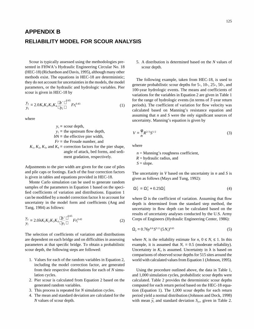
125

APPENDIX B

RELIABILITY MODEL FOR SCOUR ANALYSIS

Scour is typically assessed using the methodologies pre-sented in FHWA’s Hydraulic Engineering Circular No. 18(HEC-18) (Richardson and Davis, 1995), although many othermethods exist. The equations in HEC-18 are deterministic;they do not account for uncertainties in the models, the modelparameters, or the hydraulic and hydrologic variables. Pierscour is given in HEC-18 by

(1)

where

ys = scour depth,y1 = the upstream flow depth,

bN = the effective pier width,Fr = the Froude number, and

K1, K2, K3, and K4 = correction factors for the pier shape,angle of attack, bed forms, and sedi-ment gradation, respectively.

Adjustments to the pier width are given for the case of pilesand pile caps or footings. Each of the four correction factorsis given in tables and equations provided in HEC-18.

Monte Carlo simulation can be used to generate randomsamples of the parameters in Equation 1 based on the speci-fied coefficients of variation and distributions. Equation 1can be modified by a model correction factor λ to account foruncertainty in the model form and coefficients (Ang andTang, 1984) as follows:

(2)

The selection of coefficients of variation and distributionsare dependent on each bridge and on difficulties in assessingparameters at that specific bridge. To obtain a probabilisticscour depth, the following steps are followed:

1. Values for each of the random variables in Equation 2,including the model correction factor, are generatedfrom their respective distributions for each of N simu-lation cycles.

2. Pier scour is calculated from Equation 2 based on thegenerated random variables.

3. This process is repeated for N simulation cycles.4. The mean and standard deviation are calculated for the

N values of scour depth.

yy

K K K K by

Frs

11 2 3 4

1

0 65

10 432 0=

−.

..λ

yy

K K K K by

Frs

11 2 3 4

1

0 65

10 432 0=

−.

..

5. A distribution is determined based on the N values ofscour depth.

The following example, taken from HEC-18, is used togenerate probabilistic scour depths for 5-, 10-, 25-, 50-, and100-year hydrologic events. The means and coefficients ofvariations for the variables in Equation 2 are given in Table 1for the range of hydrologic events (in terms of T-year returnperiods). The coefficient of variation for flow velocity wascalculated based on Manning’s resistance equation andassuming that n and S were the only significant sources ofuncertainty. Manning’s equation is given by

(3)

where

n = Manning’s roughness coefficient,R = hydraulic radius, andS = slope.

The uncertainty in V based on the uncertainty in n and S isgiven as follows (Mays and Tung, 1992):

(4)

where Ω is the coefficient of variation. Assuming that flowdepth is determined from the standard step method, theuncertainty in flow depth can be calculated based on theresults of uncertainty analyses conducted by the U.S. ArmyCorps of Engineers (Hydraulic Engineering Center, 1986):

Ωy = 0.76y0.6S0.11 (5Nr)0.65 (5)

where Nr is the reliability estimate for n, 0 ≤ Nr ≤ 1. In thisexample, it is assumed that Nr = 0.5 (moderate reliability).Uncertainty in K3 is assumed. Uncertainty in λ is based oncomparisons of observed scour depths for 515 sites around theworld with calculated values from Equation 1 (Johnson, 1995).

Using the procedure outlined above, the data in Table 1,and 1,000 simulation cycles, probabilistic scour depths werecalculated. Table 2 provides the deterministic scour depthscomputed for each return period based on the HEC-18 equa-tion (Equation 1). The 1,000 scour depths for each returnperiod yield a normal distribution (Johnson and Dock, 1998)with mean ys and standard deviation Sys, given in Table 2.

Ω Ω ΩV n S2 2 20 25= + .

Vn

R S= φ 2 3 1 2/ /

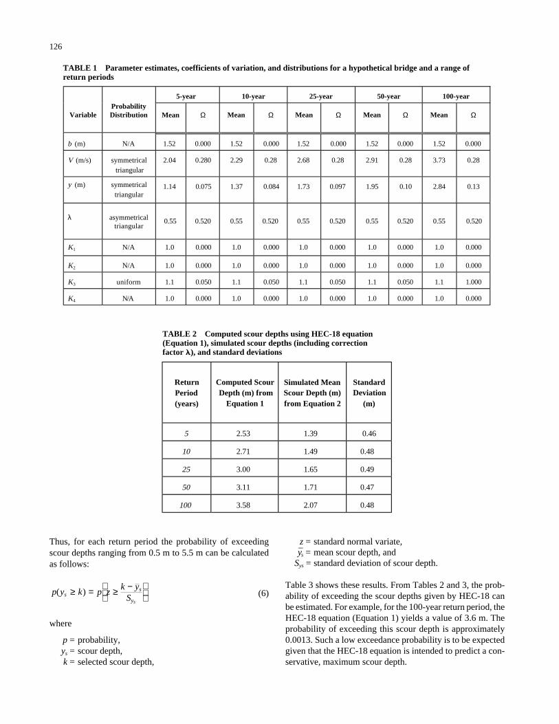
126

Thus, for each return period the probability of exceedingscour depths ranging from 0.5 m to 5.5 m can be calculatedas follows:

(6)

where

p = probability,ys = scour depth,k = selected scour depth,

p y k p zk y

Sss

ys

( )≥ = ≥ −

z = standard normal variate,ys = mean scour depth, and

Sys = standard deviation of scour depth.

Table 3 shows these results. From Tables 2 and 3, the prob-ability of exceeding the scour depths given by HEC-18 canbe estimated. For example, for the 100-year return period, theHEC-18 equation (Equation 1) yields a value of 3.6 m. Theprobability of exceeding this scour depth is approximately0.0013. Such a low exceedance probability is to be expectedgiven that the HEC-18 equation is intended to predict a con-servative, maximum scour depth.

TABLE 1 Parameter estimates, coefficients of variation, and distributions for a hypothetical bridge and a range ofreturn periods

5-year 10-year 25-year 50-year 100-year

VariableProbabilityDistribution Mean Ω Ω ΩMean Mean ΩMean ΩMean

b (m) N/A 1.52 0.000 1.52 0.000 1.52 0.000 1.52 0.000 1.52 0.000

V (m/s) symmetricaltriangular

2.04 0.280 2.29 0.28 2.68 0.28 2.91 0.28 3.73 0.28

y (m) symmetricaltriangular

1.14 0.075 1.37 0.084 1.73 0.097 1.95 0.10 2.84 0.13

λ asymmetricaltriangular

0.55 0.520 0.55 0.520 0.55 0.520 0.55 0.520 0.55 0.520

K1 N/A 1.0 0.000 1.0 0.000 1.0 0.000 1.0 0.000 1.0 0.000

K2 N/A 1.0 0.000 1.0 0.000 1.0 0.000 1.0 0.000 1.0 0.000

K3 uniform 1.1 0.050 1.1 0.050 1.1 0.050 1.1 0.050 1.1 1.000

K4 N/A 1.0 0.000 1.0 0.000 1.0 0.000 1.0 0.000 1.0 0.000

TABLE 2 Computed scour depths using HEC-18 equation(Equation 1), simulated scour depths (including correctionfactor ), and standard deviations

ReturnPeriod(years)

Computed ScourDepth (m) from

Equation 1

Simulated Mean Scour Depth (m)from Equation 2

StandardDeviation

(m)

5 2.53 1.39 0.46

10 2.71 1.49 0.48

25 3.00 1.65 0.49

50 3.11 1.71 0.47

100 3.58 2.07 0.48

127

REFERENCES FOR APPENDIX B

Ang, A.H-S., and Tang, W.H. (1984). Probability Concepts in Engi-neering Planning and Design, Volume II. Wiley and Sons, NY.

Hydraulic Engineering Center (1986). Accuracy of Computed WaterSurface Profiles. U.S. Army Corps of Engineers, Davis, CA.

Johnson, P.A. (1995). Comparison of Pier Scour Equations UsingField Data. Journal of Hydraulic Engineering, ASCE, 121(8);pp. 626–629.

Johnson, P.A., and Dock, D.A. (1998). Probabilistic Bridge ScourEstimates. Journal of Hydraulic Engineering, ASCE, 124(7); pp.750–755.

Mays, L.W., and Tung, Y.K. (1992). Hydrosystems Engineeringand Management. McGraw-Hill, Inc.

Richardson, E.V., and Davis, S.R. (1995). Evaluating Scour atBridges, 3rd edition. Report No. FHWA-IP-90-017, HydraulicEngineering Circular No. 18, Federal Highway Administration,Washington, DC.

TABLE 3 Exceedance probabilities for selected scour depths

SelectedScour

Depth, k (m)

5-year 10-year 25-year 50-year 100-year

0.5 0.9735 0.9804 0.9905 0.9950 0.9993

1 0.8017 0.8463 0.9077 0.9346 0.9848

1.5 0.4055 0.4917 0.6202 0.6725 0.8705

2 0.0924 0.1440 0.2375 0.2686 0.5364

2.5 0.0079 0.0177 0.0414 0.0464 0.1721

3 2.327E-04 0.0008 0.0029 0.0030 0.0237

3.5 2.251E-06 1.411E-05 7.986E-05 6.992E-05 0.0013

4

4.5

6.998E-09 8.530E-08 8.106E-07 5.521E-07 2.475E-5

1.803E-10 3.017E-09 1.463E-09 1.743E-76.897E-12

5 2.109E-15 1.321E-13 4.075E-12 1.288E-12 4.335E-10

5.5 0 0 0 0 3.773E-13

128

APPENDIX C

RELIABILITY ANALYSIS OF THREE-SPAN BRIDGE MODEL

1. TRADITIONAL SCOUR EVALUATIONAPPROACH

The AASHTO LRFD specifications (1994) state that “amajority of bridges that have failed in the United States andelsewhere have failed due to scour.” This is confirmed byShirole and Holt (1991), who observed that over the last 30years, more than 1,000 of the 600,000 U.S. bridges have failedand that 60% of these failures are due to scour while earth-quakes accounted for only 2%. Of course, there are many morebridges that are posted or otherwise taken out of service dueto their inadequate strengths (e.g., due to deterioration, lowrating, fatigue damage, etc.); nevertheless, scour is consid-ered a critical cause of failure because its occurrence oftenleads to total collapse. For these reasons, developing meth-ods for the design and maintenance of bridge foundations forscour is currently considered a top priority for agencies con-cerned with the safety of bridges.

The AASHTO LRFD specifications require that scour atbridge foundations be designed for the 100-year flood stormsurge tide or for the overtopping flood of lesser recurrenceinterval. The corresponding 100-year design scour depth atbridge foundations is determined following the procedurerecommended by FHWA, using what is known as “HEC-18”(Hydraulic Engineering Circular No. 18 [Richardson andDavis, 1995]). The foundation should then be designed takeninto consideration the design scour depth. This is achievedby, for example, placing the footings below the scour depth,ensuring that the lengths of piles and pile shafts extend beyondthe scour depth, and verifying that the remaining soil depthafter scour provide sufficient resistances against shear fail-ures and overturning.

HEC-18 recognizes that the total scour at a highway cross-ing is comprised of three components:

1. Long-term aggradation and degradation,2. Contraction scour, and3. Local scour.

Aggradation and degradation are long-term elevation changesin the streambed of the river or waterway caused by erosionand deposition of material. Contraction scour is due to theremoval of material from the bed and the banks of a channel,often caused by the bridge embankments encroaching ontothe main channel.

Local scour involves the removal of material from aroundbridge piers and abutments. It is caused by an acceleration offlow around the bridge foundation that accompanies a rise inwater levels that may be due to floods and other events. Local

scour and contraction scour can be either clear-water or live-bed. Live-bed conditions occur when there is a transport ofbed material in the approach reach. Clear-water conditionsoccur when there is no bed material transport. Live-bed localscour is cyclic in nature as it allows the scour hole that devel-ops during the rising stage of the water flow to refill duringthe falling stage. Clear-water scour is permanent because itdoes not allow for a refill of the hole.

In this research effort, attention was focused on local live-bed scour around bridge piers that, because of its cyclicalnature, is the most unpredictable type of scour. For localscour around bridge piers, HEC-18 recommends the use ofthe following design equation to predict the 100-year designscour depth:

(1)

where

ymax = the maximum depth of scour;Y0 = the depth of flow just upstream of the

bridge pier excluding local scour;K1, K2, K3 and K4 = coefficients that account for the nose

shape of the pier, the angle betweenthe direction of the flow and the direc-tion of the pier, the streambed condi-tions, and the bed material size;

D = the pier diameter, andF0 = the Froude number defined as follows:

(2)

where V is the mean flow velocity at the pier, and g is theacceleration due to gravity.

The process that is followed to calculate the 100-yeardesign (or nominal) scour depth for a bridge pier is as follows:

1. Use statistical data on flood events for the bridge siteto obtain the expected maximum 100-year flood dis-charge rate.

2. Perform a hydraulic analysis to obtain the correspond-ing expected maximum 100-year flow velocity, V, andthe 100-year stream flow depth, y0.

3. Use the information from Step 2 to calculate the Froudenumber.

F Vgy0

00 5=

( ) .

y y K K K K Dy

Fmax

..=

2 0 1 2 3 4

0

0 65

00 43

129

4. Use information on pier geometry, streambed condi-tions and angle of attack, and streambed material to cal-culate D, K1, K2, K3 and K4.

5. Substitute the values obtained into the HEC-18 Equa-tion 1 to calculate the 100-year design scour depth forthe bridge under consideration.

The objective of this project, NCHRP Project 12-48, is to cal-ibrate load factors for the scour extreme event and the com-bination of scour with other extreme events such as earth-quakes, winds, and ship collisions. The calibration should beperformed using reliability methods to be compatible withthe AASHTO LRFD specifications. The calibration processrequires the evaluation of the reliability inherent in currentdesign practice. The steps of the calibration process involve

1. “Designing” a number of typical bridges to satisfy cur-rent specifications.

2. Finding the inherent reliability in these designs.3. Finally, calibrating a set of load factors to ensure that

bridges designed with these factors will satisfy a targetreliability that will be determined based on the experi-ence gained from previous designs.

This appendix focuses on developing a model for calibratingload factors for bridges subjected to the combination of scourand earthquake forces. Current design practice for scour usesthe HEC-18 equations published by FHWA. This sectionillustrates the use of HEC-18 for finding the scour depth at abridge pier. The methods will subsequently be used to developa model to study the reliability of bridges subjected to scour

and a model to study the reliability of bridges subjected to thecombined effects of scour and earthquake forces.

1.1 Illustrative Example

To illustrate the use of the HEC-18 equation to find thescour depth at a bridge pier, we assume that we are to designa bridge for the 100-year scour. The bridge is to be locatedover a 220-ft wide segment of a river, and the bridge will havethe configuration shown in Figure 1.

The bridge is constructed over a 200-ft wide river. To obtainrealistic results for different possible discharge rates, data fromdifferent small size rivers are used and design scour depths arecalculated for each of these river discharge rates. The riverschosen for this analysis consist of the following: (1) SchohaireCreek in upstate New York, (2) Mohawk River in upstate NewYork, (3) Cuyahoga River in northern Ohio, (4) Rocky Riverin Ohio, and (5) Sandusky River in Ohio. Data on the peakannual discharge rates for each of the five rivers was obtainedfrom the U.S. Geological Survey (USGS) website. Lognormalprobability plots and Kolmogorov–Smirnov (K-S) goodness-of-fit tests showed that the peak annual discharge rate, Q, forall five rivers can be well modeled by lognormal probabilitydistributions. The mean of the log Q and its standard devia-tion were calculated using a maximum likelihood estimator.This data are provided in Table 1, along with the K-S maxi-mum difference in cumulative distribution, Dn. Dn* is the K-Smaximum difference between the measured cumulative prob-ability and expected probability value. More than 60 datapoints were available for each of the five rivers. This indicates

60’ 100’ 60’

10”

6’

3’

y s

22’

Figure 1. Profile of example bridge.

TABLE 1 Probability models for five rivers

River Log Q Slog Q *nD

Schohaire 9.925 0.578 0.067 Mohawk 9.832 0.243 0.068 Sandusky 9.631 0.372 0.086 Cuyahoga 9.108 0.328 0.065 Rocky 9.012 0.378 0.049

130

that the lognormal distribution is acceptable for a significantlevels α = 20 percent.

In this example, we will assume that the width of the chan-nel at the bridge site is permanently set at 220 ft, as shown inFigure 1. The rate of flow, Q, at a given point in time is relatedto the cross sectional area of the stream, A0, and the streamflow velocity, V, by

Q = A0V. (3)

For a rectangular cross section with a constant width, b, andflow depth, Y0, the relationship becomes

Q = by0V. (4)

The flow velocity, V, depends on the flow depth, y0. The rela-tionship between the flow velocity, V, and flow depth, y0, canbe expressed using Manning’s equation:

(5)

where

n = the Manning roughness coefficient, which would varybetween 0.025 to 0.035 for earth (respectively forgood condition and for weeds and stones);

R = the hydraulic radius;S = the slope of the bed stream; andΦ = an empirical factor equal to 1.486 when using U.S.

units (ft and sec).

For SI units, F = 1.0. For the problem described in Figure 1,the hydraulic radius, R, can be calculated by

(6)

In this illustration, we will assume a slope of S = 0.2%. Usingthe equations given above, the relationship between the flowrate Q and the flow depth y is given from the equation

(7)Q byn

byb y

S=+

0

0

0

2 31 2

2Φ /

/

Rby

y=

+0

02.

Vn

R S= Φ 2 3 1 2/ /

where the following is input data:

b = 220 ft,Φ = 1.486,n = 0.025, andS = 0.2%.

For the discharge rate data for each river shown in Table 1,the flow depth for the 100-year flood can be calculated as y0

along with the corresponding velocity v. Given this informa-tion and the geometric data of the river and the bridge pier,the maximum design scour depth can be calculated fromEquation 1. In this example, it is assumed that the round nosepier is aligned with the flow and that the bed material is sand.HEC-18 then recommends that the factors K1, K2, and K4 allbe set equal to 1.0. For plane bed condition, K3 is equal to 1.1.Using Equation 1 with the column diameter of D = 6 ft, thedesign scour depth is obtained for each river as shown inTable 2.

1.2 Discussion

To study the safety of bridges accounting for the combinedeffect of scour and other extreme events, we need to know theextent of scour for different flood intensities, and we also needto know how the scour depth varies with time. This includesthe time it takes for the flood to produce the maximum scourand the duration of the foundation exposure after the occur-rence of scour before refill. Time becomes an important pa-rameter because it controls the probability of having a simul-taneous occurrence of scour and other events.

The HEC-18 approach has been used extensively for prac-tical design considerations although the HEC-18 empiricalmodel provides conservative estimates of scour depths and isknown to have the following limitations:

1. The HEC-18 equation is based on model scale experi-ments in sand. In a recent evaluation against full-scaleobservations from 56 bridge sites, it was found to vastlyover-predict the scour depth (Landers and Mueller,1996). A comparison between the HEC-18 equationand the measured depths are illustrated in Figure 2,which is adapted from Landers and Mueller (1996).

TABLE 2 Design scour depth for each river

River Q 100-year

(ft3/sec) V

(ft/sec) Y0-flood depth (ft)

Ymax-scour depth (ft)

Schohaire 78,146 17.81 20.56 17.34 Mohawk 32,747 12.87 11.78 13.99 Sandusky 36,103 13.35 12.52 14.33 Cuyahoga 19,299 10.5 8.45 12.26 Rocky 19,693 10.58 8.56 12.32

131

2. Once a flood begins, it takes a certain amount of time forthe full extent of erosion to take effect. Thus, if the floodis of a short duration, the maximum scour depth may notbe reached before the flood recedes. On the other hand,prior floods may have caused partial erosions accelerat-ing the attainment of the maximum scour depth. HEC-18 does not predict the length of time required for themaximum scour depth to be reached and assumes thatthe maximum depth is always reached independent ofthe flood duration and the level of scour incurred byprior floods.

3. The HEC-18 model does not distinguish between live-bed scour and clear-water scour in terms of the timerequired to reach equilibrium scour depth and the dif-ferences in the expected magnitudes of scour depthsfor these different phenomena (Richardson and Davis,1995).

4. HEC-18 was developed based on experimental dataobtained for sand materials. Some work is in progressto extend the use of HEC-18 for both sand and claystreambed materials although it is known that thesematerials behave differently (Briaud et al., 1999).

5. The usual assumption is that scour is deepest near thepeak of a flood, but may be hardly visible after flood-waters recede and scour holes refill with sediment.However, there are no known methods to model howlong it takes a river to back-fill the scour hole. Refill canoccur only under live-bed conditions and depends onthe type and size of the transported bed material (i.e.,sand or clay). In any case, even if refill occurs, it will takea considerable time for the refill material to consoli-date enough to restore the pier foundation to its initialstrength capacity. Although such information is not pre-cisely available, a number of bridge engineers have sug-gested that periods of 2 to 3 months are reasonable forclay materials with longer periods required for sands.

6. Based on the observations made above, it is evident thatusing the 100-year flow velocity and flow depth in theHEC-18 equations does not imply that the annual prob-ability of failure will be 1/100. This is primarily due tothe inherent conservative bias associated with the HEC-18 equation. In fact, based on observed scour depths at515 sites, Johnson (1995) has shown that the HEC-18equation produces scour depth estimates that are on theaverage 1.8 times higher than the measured values. Thisshows that the HEC-18 equation has a bias equal to 0.55(1/1.8). The observed differences between predictionsand measurements produced a coefficient of variation(COV; standard deviation/mean) of 52%. Figure 2 showsthat these estimates are reasonable when compared withthe data collected by Landers and Muller (1996).

Based on the observations made herein, an appropriate reli-ability model for the safety analysis of a bridge pier under theeffect of scour is proposed, as illustrated in Section 2 of thisreport. This model is based on the work presented in Appen-dix B of the interim report for NCHRP Project 12-48.

2. RELIABILITY ANALYSIS FOR SCOUR

The HEC-18 model stipulates that previous levels of scourat the site do not affect the scour depth produced by a givenflood. Hence, the maximum scour in a given return periodis a function of the maximum flood observed in that periodand is not affected by previous smaller floods that may haveoccurred within that same period. In addition, the HEC-18model assumes that the flood duration is always long enoughfor the full scour depth corresponding to the flood velocityto be reached.

Although the scour hole is normally assumed to refill as thescour-causing flood recedes, the available literature does notprovide precise information on how long it normally takes forthe foundation to regain its original strength. This is believedto depend on the type of material being deposited by live-bedstreams. For example, cohesive materials such as clays maytend to regain their strength within a short period of time(perhaps 2 to 3 months). On the other hand, fine sands maytake much longer to consolidate and regain their originalstrengths. As a compromise, for this illustrative example,we will assume that it will take about 6 months (1/2 year) fora foundation to regain its original strength. We will assumethat the scour depth produced by the maximum yearly floodwill remain at its maximum value for this half-year period.This assumption will also indirectly account for the effectsof smaller floods within that period of time. In the proposedmodel, we will also assume that the scour depth will bereached instantaneously as the flood occurs and that the flood-ing period is always long enough for the maximum scourdepth to be reached.

Using these assumptions, the proposed model for occur-rence of scour can be represented as shown in Figure 3. T is

Figure 2. Comparison of HEC-18 predictions withobserved scour depths.

132

the lifetime of the bridge (e.g., 75 years), t is equal to theduration of the maximum scour (1/2 year) for each time unit(1 year). n is the number of scour occurrences within the timeperiod T (or number of scour repetitions). For the 75-yeardesign life of a bridge, n = 75, assuming one flooding seasonper year.

The model represented in Figure 3 can be used to calculatethe reliability of a foundation subjected to scour alone or tothe combination of scour and other extreme events. The reli-ability calculations for scour alone are illustrated in Section2.1 in this appendix. The reliability calculations for the com-bination of scour and earthquake loads are illustrated in Sec-tion 5. In order to illustrate the load combination problem, areliability model for earthquake alone is needed. Such a modelis presented in Section 4.

2.1 Reliability Analysis for Scour Alone

The model used herein for the reliability analysis of abridge foundation subjected to scour alone is based on theexample provided in Appendix B of the interim report forNCHRP Project 12-48. The calculations use the followingassumptions:

1. The probability distribution for the maximum 1-yearflood is expressed as FQ(x), which gives the cumulativeprobability that the 1-year discharge volume, Q, is lessthan x. The cumulative probability distribution of themaximum 1-year discharge volume Q follows a log-normal distribution. This is based on probability plotsand K-S goodness-of-fit tests.

2. A 75-year design life (return period) is assumed inorder to be consistent with the AASHTO LRFD speci-fications.

3. The maximum 75-year flood discharge has a cumula-tive probability distribution FQ75 (x) related to the prob-ability distribution of the 1-year maximum dischargeby

FQ75(x) = FQ(x)75. (8)

Equation 8 assumes independence between the floodsobserved in different years. This assumption is consis-tent with current methods to predict maximum floods.

4. For a specific discharge rate Q, the corresponding val-ues for the flow velocity V and flow depth y0 can be cal-culated by solving Equation 7 for y0 and then usingEquation 5 to find V.

5. It is noted that determining the appropriate Manningroughness coefficient (n in Equations 5 and 7) is asso-ciated with a high level of uncertainty. Therefore, inthis example, we will assume that n is a random variablewith a mean value equal to 0.025 (the recommendedvalue for smooth earth surfaces) and a coefficient ofvariation equal to 28%. The 28% COV was adaptedfrom the Hydraulic Engineering Center (1986), whichrecommends that n follow a lognormal distribution witha COV ranging from 20% to 35% (with an average valueof 28%). It is herein assumed that the slope S is knownand, thus, the uncertainties in V are primarily due to theuncertainties in determining n.

6. For any set of values for V and y0, one can calculate theFroude number from Equation 2 and substitute thesevalues into Equation 1 to find the 100-year design scourdepth. Equation 1, however, as explained earlier, givesa safe value for the depth of scour. The average valuewas found by Johnson (1995) to be about 0.55 times thenominal value (bias value is 0.55). Also, the ratio of thetrue scour value over the predicted value has a COV of52%. This bias is represented by a modeling parameterλsc. Thus, the true scour value is given by an equationof the form

(9)

7. It should be noted that Johnson (1995) also recom-mends that the factor K3, representing the effect ofstreambed condition, be treated as random variablewith a bias equal to 1.0 and a COV equal to 5%.

8. Data on the type of the probability distributions for λsc

and K3 are not available. In the interim report for thisproject, Johnson proposed to use triangular distribu-tions. It is herein assumed that n will follow a lognor-mal distribution as recommended by the HydraulicEngineering Center (1986). This will ensure that n doesnot take values less than 0. On the other hand, becauseit is unlikely that λsc and K3 will have upper or lowerbounds, we shall herein assume that these two randomvariables follow normal (Gaussian) distributions. Notethat triangular distributions where assumed in theinterim report for both these variables. A sensitivityanalysis will be performed at a later stage of this proj-ect to study how these assumptions will affect the finalresults.

y y K K K K Dy

Fscmax

..=

2 0 1 1 1 1

0

0 65

00 43λ

t t t t=1/2 year t t t t tt t t

T

n=T/2t

Time in years

Sco

ur d

epth

Figure 3. Representation of proposed scour model.

133

The information provided above can be used in a simulationprogram to find the probability that the scour depth in a 75-year period will exceed a given value ycr. A summary of theinput data used in a Monte Carlo simulation program that cal-culates the probability that the actual scour depth will exceeda critical value is shown in Table 3.

The probability that ymax will exceed a critical scour depth,ycr, is calculated for different values of ycr as shown in Figure 4for all five rivers. This data are also summarized in Table 4.The results of the simulation can be summarized as shown inTable 4 for the five rivers. It is observed that the safety indeximplied in current scour design procedures is on the order of1.40 to 1.50, which is much lower than the 3.5 safety indexused as the basis for the calibration of the load factors for thecombination of live and dead loads.

Table 5 gives the load factor that should be applied on thescour design equation in order to produce different values ofreliability indexes. For example, if a target reliability indexof βtarget = 3.50 is desired, then the average load factor thatshould be used in designing bridge foundations for scourshould be equal to 1.69. Similarly, if a reliability index βtarget =2.50 is to be used as the target index for the design of bridge

foundations for scour, then the load factor should be equal to1.32. This means that a “load” (safety factor) equal to 1.69 tosatisfy a target index of 3.5 or equal to 1.32 to satisfy a targetindex of 2.50 should further multiply the scour depth obtainedfrom Equation 1. The load factors for other target safety indexvalues ranging from 4.0 to 2.0 are provided in Table 5.

2.2 Final Remarks

The reliability calculations shown above assumed a deter-ministic value of ycr. In general the critical depth, ycr, that willproduce the failure of the foundation is a random variablethat depends on the foundation type, soil properties, and thetype of loading (lateral or vertical) applied on the structure.For example, under the effect of lateral loads, pile founda-tions may fail in shear or in bending. Probability of failurewould increase in the presence of scour that extends themoment arm of the lateral load. In addition, scour woulddecrease the depth of the remaining soil available to resist theapplied moment and shear forces. On the other hand, when adynamic analysis is performed, it is observed that the pres-ence of scour reduces the stiffness of the bridge foundation

TABLE 3 Input data for reliability analysis for scour alone

Variable Mean value COV Distribution Type Q—maximum 75-yr discharge rate As provided in Table 1 As provided in Table 1 Lognormal λQ modeling variable for Q 1 5% Normal n Manning roughness 0.025 28% Lognormal λ sc modeling variable 0.55 52% Normal K3 Bed condition factor 1.1 5% Normal

Probability of scour depth exceedance

0

0.1

0.2

0.3

0.4

0.5

0.6

0.7

0.8

0.9

1

0 5 10 15 20 25 30scour depth (feet)

Pro

bab

ility

of

exce

edan

ce

SchohaireSanduskyCuyahogaRockyMohawk

Figure 4. Probability that actual scour will exceed critical depths.

134

thus creating a more flexible system that often leads to areduction in dynamic loads. The example solved in the nextsection of this report will illustrate how the lateral load willaffect the safety of bridges for different failure modes.

The controlling random variable for the reliability analysisis the modeling factor λsc, which has a high COV of 52%. ThisCOV is higher than that of the maximum 75-year flood, whichis about 15%. It should be noted that the analysis performedfor scour alone produces a reliability index and probability offailure values that are totally independent of the time periodduring which the scour hole is at its maximum depth. Theeffect of the scour duration will be important as we study thereliability of bridge piers due to the combined effects of scourand other loads. Section 3 will analyze the bridge described inFigure 1 for earthquake loads using current analysis meth-ods. Section 4 will develop a model for the reliability analy-sis of bridge piers subjected to earthquake loads alone. Sec-tion 5 will demonstrate the reliability analysis for thecombination of earthquake loads and scour.

3. ANALYSIS OF BRIDGE FOR EARTHQUAKE LOADS

In this appendix, we are illustrating the case in which scouris to be combined with seismic forces. In order to study thecombination problem, we first perform a deterministic analy-sis of the bridge under the effect of seismic forces to determinethe nominal design forces and moments. In Section 4, the reli-ability of the column subjected to seismic forces alone isexecuted. In Section 5, the reliability analysis is expanded todemonstrate how the combination of scour and earthquakes

will affect the reliability of the column and the foundation. Thereliability analysis will be used to develop load factors that willbe calibrated to achieve consistent target reliability levels. Afirst attempt on the calibration is presented in Section 6.

3.1 Bridge Geometric Properties

The bridge example studied in this section consists of threespans (60 ft, 100 ft, 60 ft) as illustrated in Figure 1 of Section1.1. The bridge has two bents, each of which is formed by a6-ft-diameter column. The weight applied on each bent iscalculated to be 1,527 kips divided as follows: superstructureweight = 979 kips, weight of substructure = 322 kips, andweight of wearing surface = 2.46 kip/ft. Following currentpractice, the tributary length for each column is 91.9 ft where50 ft is 50% of the distance between the columns and 41.9 ftis 70% of the distance between the column and the externalsupport. This assumes that the lateral connection of the super-structure to the abutments will not break because of the earth-quake lateral motions. The clear distance between the base ofthe column and the center of the superstructure is 25 ft. Thefoundation consists of a pile shaft (pile extension) that extends50 ft into the soil. The soil is assumed to have an elastic mod-ulus of Es = 10,000 psi corresponding to moderately stiffsand. The point of fixity of the floating foundation can be cal-culated using the relationship provided by Poulos and Davis(1980), given as follows:

(10)LL

eL

LL

K I eL

Ie eR H M

+

= +( )3 2

1 5 3. ρ ρ

TABLE 5 Design scour depths required to satisfy target reliability levels

Target index β = 4.0 β = 3.5 β = 3.0 β = 2.5 β = 2.0

Required depth (ft) Depth

Load factor Depth

Load factor Depth

Load factor Depth

Load factor Depth

Load factor

River Schohaire 33.5 1.90 30.0 1.73 26.0 1.50 23.0 1.33 20.0 1.15 Mohawk 26.0 1.86 23.0 1.64 20.5 1.46 18.5 1.32 16.0 1.14 Sandusky 26.5 1.85 24.0 1.68 21.0 1.47 19.0 1.33 17.0 1.19 Cuyahoga 22.0 1.79 20.5 1.67 18.0 1.46 16.0 1.30 14.0 1.14 Rocky 23.0 1.87 21.0 1.71 18.0 1.46 16.0 1.30 14.0 1.14 Average 1.85 1.69 1.46 1.32 1.15

TABLE 4 Summary of simulation results

River

Average Q75yr (Q for 75 years) (ft3/sec)

COV of Q75yr

Average ys75 (max.scour

depth in 75 yrs)

COV of Ys75

Design depth (ft)

Reliability index β

Schohaire 85,000 29% 9.8 52% 17.3 1.40 Mohawk 34,000 12% 7.8 51% 14.0 1.51 Sandusky 38,000 18% 8.0 51% 14.3 1.41 Cuyahoga 20,000 16% 6.9 51% 12.3 1.42 Rocky 21,000 19% 6.9 51% 12.3 1.40

135

where

Le = the effective depth of the foundation (distance fromground level to point of fixity);

L = the actual depth;e = the clear distance of the column above ground level;

KR = the pile flexibility factor which gives the relativestiffness of the pile and soil;

IρH = the influence coefficient for lateral force; andIρM = the influence coefficient for moment.

The pile flexibility factor is given as follows:

(11)

If the pile is made of 4,000 psi concrete, then Ep equaling3600 ksi (= 57[4000]1/2) and the diameter of the columnbeing D = 6 ft results in a moment of inertia Ip = 63.62 ft4

(= πr4/4). Thus, for a pile length of 50 ft, the pile flexibilitybecomes

(11′)

The charts provided by Poulos and Davis (1980) show thatfor KR = 0.0037, the influence coefficients IρH and IρM arerespectively on the order of 5 and 15. This will produce anequation of the following form:

(10′)

where the value of e = 25 ft, which is the clear height of thecolumn.

The root of this equation produces a ratio of Le /L = 0.35,resulting in an effective depth of 18 ft below ground surface.Thus the effective total column height until the point of fix-ity becomes 25 ft + 18 ft = 43 ft.

For transverse seismic motion, the bent is assumed to befixed at the base of the effective pile depth and free on thetop. Thus, the bent stiffness is

(12)

where

H = the effective column height (H = e + Le),E = the column’s modulus of elasticity, andI = the moment of inertia.

For typical concrete columns, E equals 3,600 ksi. For a cir-cular column with a diameter of D = 6 ft, the moment ofinertia is

K EIHbent = 3

3

L Le e

501 5 25

50 503 0 0037 5 25

5050

3 2

+

= × × +( ). .

KE IE LR

p p

s= = ×

×=4

3 600 000 63 640 037

, ,10,000 504

.. .

KE IE LR

p p

s= 4 .

(13)

For a height equal to 45 ft, Equation 13 gives the bent stiff-ness as follows:

(12′)

The natural period of the bent system, T is

(14)

where

ω = the circular frequency of the system;M = the mass (M = W/g where W is the weight and g is the

acceleration of gravity); andK = the stiffness.

According the AASHTO LRFD specifications, the elasticseismic response coefficient C is given by

(15)

where

A = the acceleration coefficient (the seismic accelerationas a multiple of the acceleration of gravity),

S = the soil type parameter, andT = the natural period of the system.

The AASHTO LRFD specifications (Figure 3.10.2-2 of themanual) provide maps that give seismic acceleration for dif-ferent regions of the United States. For example, for bridgesto be located in the New York City area, the map of the accel-eration coefficients shows a value of A on the order of 15%to 18% of g. Current trends in earthquake design of highwaybridges are favoring the use of the National Earthquake Haz-ards Reduction Program (NEHRP) spectra, and a new earth-quake design specification for bridges is proposing to use thesame NEHRP spectra developed for buildings. For this rea-son, this appendix is based on using the NEHRP spectra ratherthan the current AASHTO specifications. The sections belowillustrate the application of the NEHRP approach for thedesign of the bridge illustrated in Figure 1 of Section 1.1.

3.2 Earthquake Intensity

The USGS mapping project gives the peak ground acceler-ations (PGAs) at bedrock level and the corresponding spectral

C AST

A= ≤1 2 2 52 3. ./

T MK

= = =

=

2 2 21527 32 2

1244

2πω

π π kip ft kip/ft

1.23 sec

/ . /sec

K EIHbent = = × × ×

=

3 3 3600 144 63 6443

124

3

4

3k/in ft /in ft

ft

4 kip/ft

2 2 2 .( )

.

I r ft= = =π π4 44

434

63 64. .

136

values for 10%, 5%, and 2% probability of exceedance in 50years for points throughout the United States. The spectralaccelerations are given for periods of 0.2, 0.3, and 1.0 seccorresponding to the three different PGAs. Table 6 liststhese values for the areas with the following zip codes: 10031in New York City, 38101 in Memphis, 55418 in St. Paul,98195 in Seattle, and 94117 in San Francisco. The spectralaccelerations give the accelerations of the mass of a single-degree-of-freedom system that is supported by a system thathas a natural period of 0.2, 0.3, or 1.0 sec when the acceler-ation at the base of the system is equal to the correspondingPGA. The values shown in Table 6 are in %g where g is theacceleration due to gravity. Table 6 shows the accelerationsfor three different probabilities of exceedance, namely 10%in 50 years, 5% in 50 years, and 2% in 50 years. For exam-ple, the 2% in 50 years corresponds to an earthquake returnperiod of 2,500 years. The 10% in 50 years corresponds to areturn period of 500 years. These return periods are normallyused as the bases of current bridge design practice.

3.3 NEHRP Earthquake Response Spectrum

The spectral accelerations provided in Table 6 are for single-degree-of-freedom (SDOF) systems founded on bedrock.The values are given for only three natural periods—0.2, 0.3,

and 1.0 sec—in addition to the PGA. NEHRP has proposeda method to use the information provided in Table 6 todevelop acceleration response spectra that are valid for vari-ous soil conditions and for systems with different naturalperiods. The NEHRP response spectra can be described by acurve with the shape shown in Figure 5. In Figure 5, Sa is thespectral acceleration, T is the natural period of the system, SDs

is the maximum spectral acceleration, and SDl is the spectralacceleration for a period of T = l sec. All spectral accelera-tions are given as function of g, the acceleration due to grav-ity. T0 gives the period at which the maximum spectral accel-eration is reached. Ts gives the period at which the spectralacceleration decreases below the maximum value. When theperiod T is less than T0, the spectral acceleration increaseslinearly. When the period T is greater than Ts, the spectralacceleration is inversely proportional to T. The values of SDs

and SDl, as well as T0 and Ts, are calculated from the spectralaccelerations given in Table 6 and the soil properties asdescribed further below.

The first step in the earthquake analysis process is todevelop the spectral response curve of Figure 5. This requiresthe identification of the foundation soil type. Having a mod-ulus of elasticity on the order of 10,000 psi would classify thesite condition as stiff soil (NEHRP Soil Category D). Thisinformation will be used to obtain the site coefficients (or siteamplification factors).

For a 500-year return period (10%PE in 50 years), themapped spectral acceleration, Ss, for the short period of T = 0.2sec is taken from Table 6 for each of the five sites. Similarly,the spectral acceleration SI for a period of T = l sec is obtainedfrom Table 6 for each site. The site coefficients are obtainedfrom the NEHRP provisions as Fa for short periods and Fv for1 sec from Table 4.1.2.4.a and 4.1.2.4.b of NEHRP (1997).Thus, the maximum earthquake spectral response accelera-tions for short period (0.2 sec) SMS and for the 1-sec period SM1

adjusted for the proper soil profile are obtained from

SMS = Fa SS and SM1 = Fv S1. (16)

NEHRP allows for a 2/3 (= 0.667) correction on the maximumearthquake accelerations. Thus, the critical amplitudes on theresponse spectrum are

TABLE 6 Probabilistic ground motion values, in %g, forfive sites (based on USGS website)

Site 10% PE in

50 yr 5% PE in

50 yr 2% PE in

50 yr S.Francisco PGA 52.65 65 76.52 0.2 sec SA 121.61 140.14 181 0.3 sec SA 120.94 140.44 181.97 1.0 sec SA 57.7 71.83 100.14 Seattle PGA 33.77 48.61 76.49 0.2 sec SA 75.2 113.63 161.34 0.3 sec SA 62.25 103.36 145.47 1.0 sec SA 22.06 32.23 55.97 St. Paul PGA 0.76 1.31 2.5 0.2 sec SA 1.82 3.17 5.63 0.3 sec SA 1.61 2.72 4.98 1.0 sec SA 0.73 1.38 2.66 New York PGA 6.32 11.92 24.45 0.2 sec SA 12.59 22.98 42.55 0.3 sec SA 9.42 16.64 31.17 1.0 sec SA 2.85 5.11 9.4Memphis PGA 13.92 30.17 69.03 0.2 sec SA 27.46 58.71 130.03 0.3 sec SA 20.38 43.36 110.62 1.0 sec SA 6.46 15.47 40.74

Sa

SDs Sa=SDt/T

SDt

T0 Ts 1.0 sec Period T

Figure 5. NEHRP design response spectrum.

137

SMS = 0.667SMS = 0.667FaSS and(17)

SM1 = 0.667SM1 = 0.667FV S1.

All spectral values are given in function of the accelerationdue to gravity, g. Critical periods on the response spectrum(see Figure 5) are

T0 = 0.20SD1/SDS and TS = SD1/SDS (18)

The equation describing the acceleration response spectrum,Sa, shown in Figure 5 will be

(19)

For the 2,500-year return period (2%PE in 50 years), themapped maximum earthquake spectral response for short peri-ods, Ss, are also taken from Table 6, and the determination ofthe spectral curve is executed following Equations 16 through19 for each of the five sites. The site coefficients, Fa and Fv

(site amplification factors), are also obtained from the NEHRPprovisions. The maximum earthquake spectral response accel-erations adjusted for the proper soil profile are given in Table 7for the five sites studied for a natural period of T = 1.23 sec,which is the period of the system studied in this example.

3.4 Design Moment Capacity of Column

Using a response modification factor of R = 2.0 for singlecolumns of essential structures, the applied design forces andmoments are reduced by R = 2.0 to account for column duc-tility. The equivalent force on the top of the column isobtained by multiplying the weight by the spectral accelera-tion (Sa) corresponding to the natural period of T = 1.23 sec.The moment at the base of the pile shaft is obtained by multi-plying the equivalent force by the effective column height H.Thus, the final design moment in the column is obtained asfollows:

SST

T S T T

S S T T T

S ST

T T

aDS

DS

a DS s

aD

s

= + <

= < <

= >

0 6 0 400

0

0

1

. . for

for

for

(20)

The weight applied on the bridge column W is 1,527 kips.The spectral acceleration values are taken from Table 7. Theeffective height of the column, H, includes the clear heightplus the depth to the point of fixity (H = e + Le = 25 ft + 18 ft= 43 ft). Using Equation 20, the design moments for the col-umn are calculated as given in Table 8.

3.5 Check of Foundation Safety

The design of the foundation should be such that the soilmust be able to resist either the elastic forces applied on thebridge system or the forces produced from the plastic hing-ing of the column. The smaller of the two resulting forces isused for designing the depth of the bridge foundation, imply-ing that if the earthquake forces induce the formation of theplastic hinge in the column, then only the forces transmittedby the hinge need to be considered for the soil resistance. Itis only in the case in which the columns are so overdesignedthat no hinges will form in them that the soil needs to carrythe full elastic forces applied on the bridge system.

For piles in cohesionless soils, the depth of the pile bentshould be such that the soil pressure resists the applied lateralforces. Using the Broms model as described by Poulos andDavis (1980), the lateral load capacity of the soil is given by

(21)

where

γ = the soil’s specific weight;L = the depth of the foundation;D = the diameter of the foundation;e = the column eccentricity above ground level; and

Kp = Rankine’s passive pressure coefficient, given by

(22)

where φ is the angle of internal friction of the soil.

Kp = +−

11

sinsin

φφ

HDL K

e Lup=

+0 5 3. γ

MWS H

Ra

design = .

TABLE 7 Spectral accelerations, Sa, for 10% and 2% PE in 50 years for bridge column (based on NEHRP specifications)

Site 10%PE in 50 yr 2%PE in 50 yr San Francisco 0.469 0.814 Seattle 0.234 0.455 St. Paul 0.009 0.035 New York 0.037 0.122 Memphis 0.084 0.352

TABLE 8 Design moments for 10% and 2% PE in 50 years (based on NEHRP specifications)

10% PE in 50 yr

(kip-ft) 2% PE in 50 yr

(kip-ft) San Francisco 15397.5 26724.03 Seattle 7682.34 14937.88 St. Paul 295.47 1149.07 New York 1214.73 4005.32 Memphis 2757.76 11556.34

138

For design purposes, the applied lateral force resultingfrom the formation of the plastic hinge in the bridge columnis obtained from the over strength moment capacity of thecolumn, which is 1.3 times the plastic moment capacity (i.e.,1.3 times the values shown in Table 8).

If the clear column height is e = 25 ft and the effective depthto the point of fixity is Le = 18 ft with H = 43 ft (H = e + Le),then the equivalent shearing force produced in the hingeaccounting for the column’s over strength will be

(23)

where Mp is taken from Table 8. Using this information, therequired foundation depth for each site is given as shown inTable 9.

Notice that the calculations of the effective depth and theapplied moment performed above during the determinationof the column design capacity assumed a foundation depth of50 ft. The results of Table 9 show that the 50-ft depth is con-servative for most bridge sites. It is also noted that the pointof fixity for the bridge/foundation system under lateral loadsis on the order of 16 to 18 ft for all foundations exceeding 30ft in actual depth. An iterative process may be used to findthe optimum foundation depth as a function of site informa-tion. In addition to resisting the lateral load, the foundationdepth should be such that the pile be able to carry the appliedvertical loads due to the dead weight of the structure and thelive load expected during its design life. The required foun-dation depth to resist the vertical loads is calculated in Sec-tion 3.6. The reliability calculations performed in Section 4studies the effect of different column depths on the safety ofbridge columns against the failure of the column in bendingand the bearing capacity of the foundation.

3.6 Safety Check of Foundationfor Vertical Loads

In addition to carrying the horizontal load produced by theearthquake tremors, the foundation should be able to carrythe vertical loads applied on the structures including the deadweight of the superstructure and substructure as well as the

HM

Hp

applied =1 3.

vertical live load. Piles resist the vertical loads caused by thecombination of friction resistance and bearing resistance.

The friction and bearing resistances are a function of thepile dimensions and soil properties. In the case studied herein,the angle of friction for sandy soil is taken as φ = 35°, themodulus of elasticity as Es = 10,000 psi, the Poisson ratio asν = 0.3, the unit weight as γ = 60 lb/ft3, and the pile diameteras D = 6 ft. Poulos and Davis (1980) show that the verticalstress in the soil will vary linearly up to a level of z = 7 timesthe pile diameter, z = 7D. This means that the stress willvary linearly up to 42 ft below ground level, after whichpoint the stress remains constant. For saturated soils, themaximum pressure will be due to the combination of waterand soil weights, thus the maximum stress will be σv = 42 ft ×60 lb/ft3 = 2,520 lb/ft2. For bored piles with φ = 35°, the bear-ing capacity factor Nq is given by Poulos and Davis (1980) asNq = 40. Thus, the bearing capacity of the pile, Pbu , at the42-ft level and below will be as follows:

Pbu = Abσv Nq (24)

where Ab is the pile base diameter. For Ab = 28.27 ft2 (= πD2/4),σv = 2,520 lb/ft2, and Nq = 40, the bearing capacity of the pileat the 42-ft depth and below is Pbu = 2.85 × 106lb or 2,850kips. The friction force, Psu, for up to z ft in depth is given by

(25)

The value of Ks tan φ = 0.20 is provided by Poulos and Davisfor a friction angle φ = 35° and for bored piles. Thus, the fric-tion force Psu for a depth of z = 42 ft will be equal to 200 kips.After the 42-ft depth, the friction force will be a constantfunction of L − 42 ft. This means that the total friction forcewill be 200 kips + 9.50 (L − 42).

The combination of Psu and Pbu should be able to carry the applied vertical loads from the superstructure as well asthe weight of the pile. Thus, the final bearing capacity Pu isgiven as

Pu = 2,850 kips + 200 kips + 9.50 kip/ft (L − 42 ft). (26)

Given a pile of length, L, the weight of the pile will be 150lb/ft3 × L × πD2/4. The applied weight of the structure hadbeen earlier given as W = 1,527 kips.

According to the AASHTO LRFD specifications (1994),the live load applied on a continuous bridge is due to 90%of the AASHTO lane load plus 90% of the effects of twoAASHTO design trucks. The reaction at the interior supportdue to these loads are on the order of 350 kips. Using theLRFD equation with a dead load factor γd = 1.25 and a liveload factor γ1 = 1.75 results in a required bearing capacityresistance of

φPreq. = γd 1,527+ γ1 350 = 2,520 kips. (27)

PD K z

suv s= π σ φ( tan )

.2

TABLE 9 Required foundation depth based oncolumn capacity

Required foundation depth (ft) Site 10% PE in 50 yr 2% PE in 50 yr

San Francisco 34.7 43.7 Seattle 26.2 34.3 St. Paul 7.6 12.5 New York 12.8 20.2 Memphis 17.5 30.8

139

For the bearing capacity of piles in sandy soils, the AASHTOLRFD does not provide a resistance factor φ, although val-ues on the order of φ = 0.50 to 0.65 are recommended for claysoils depending on the models used for calculating the bear-ing capacity. A factor of φ = 0.80 is used when the pile bear-ing capacity is verified from load tests. By comparing Equa-tions 26 and 27, it is clear that the AASHTO LRFD criteriacan be met for a pile length L = 50 ft only if pile tests are con-ducted to verify the bearing capacity of the pile shaft or whena bell at the bottom of the caisson is provided to extend thearea. For this example, we are assuming that the 50-ft pilelength is acceptable to carry the vertical loads. A sensitivityanalysis is performed in the next section to study the effectof different pile lengths on the reliability of the bridge whensubjected to earthquake loads.

4. RELIABILITY ANALYSIS OF BRIDGEFOR EARTHQUAKES

The purpose of the analysis performed in this section is tocalculate the probability that the bridge designed in Section 3for the different moment capacities will fail under the effect ofearthquake forces within its intended 75-year design life. A 75-year return period is chosen in order to remain compatible withthe AASHTO LRFD specifications. The corresponding relia-bility index, β, will also be calculated. The objective is to studythe reliability of bridges designed following current practiceand the NEHRP specifications under the effect of earthquakeloads. In this section, the analysis is performed assuming noscour. The model is subsequently used in Section 5 to studythe reliability of bridges under the combined effects of scourand earthquake loads.

In this section, we will assume that the bridge was designedas described in the previous section to withstand the earth-quake loads observed at the five different sites identifiedabove. In order to perform the reliability analysis, we willneed to account for the uncertainties associated with each ofthe random variables that control the safety of the bridge.Assuming no scour, the random variables are identified as

1. Strength capacity of bridge column,2. Intensity of the earthquake acceleration at the site,3. Natural period of the column,4. Mass applied on the column,5. Seismic response coefficient, and6. Response modification factor.

In addition, although not treated as a random variable, thefrequency of earthquakes at the bridge site plays an impor-tant role in determining the reliability of the bridge for earth-quake risk. Other factors such as the height and diameter ofthe column and other geometric and material parameters areassociated with very small uncertainties and may be treatedas deterministic values.

4.1 Column Strength Capacity

A single-column bridge pier subjected to earthquake loadscan fail in a variety of modes. These include (1) failure dueto the applied bending moment exceeding the moment capac-ity of the column (this mode should consider the interactionbetween bending and axial loads); (2) failure in shear; and(3) failure of the foundations. In this example, the reliabilityanalysis procedure is illustrated for the failure of the columndue to the applied bending moment.

The bridge columns under combined axial load and bendingmoment are normally designed such that the design point at theinteraction curve remains below the balance point. In thisexample, we are ignoring the effects of vertical accelerationsas is common in practical cases for short- to medium-lengthbridges. Hence, the uncertainty in evaluating the vertical loadis small compared with that associated with determining thelateral forces (and bending moments). For this reason, we shallassume that the effects of the axial load on the uncertainties indetermining the moment capacity are negligible.

According to Nowak (1999), the moment capacity ofconcrete members in bending is on the average higher thanthe nominal capacity by a factor of 14% (bias 1.14), and thestandard deviation is 13%. The probability distribution ofthe moment capacity is taken to be lognormal (Nowak, 1999).The final values used in this example are those recommendedby Nowak.

4.2 Frequency of Earthquakes

We shall assume that the bridge under consideration maybe located in any of the five cities listed in Table 6. The USGSSeismic Hazard Mapping Project stipulates an earthquakeoccurrence rate for each of the areas. These values are thenused by USGS to determine the maximum annual probabil-ity curve for earthquake intensities that are discussed in thenext section.

4.3 Intensity of Earthquake Accelerations

Frequencies at which earthquakes exceed certain levels ofPGAs are provided by the USGS in two different formats:(1) plots showing the probability of exceedance of maximumyearly earthquakes versus PGAs for a number of representa-tive U.S. sites, and (2) tables giving the probability of exceed-ing given acceleration levels in 50 years. The plots are shownin Figure 6.

The frequency of exceedance in 50 years is related to themaximum yearly earthquake levels, as shown below. Forexample, if the frequency of exceeding an earthquake levelof 0.53g is given as 10% in 50 years, this indicates that theprobability that the maximum earthquake level in 50 yearswill be below 0.53g is 1.00 − 0.10 = 0.90. This can be repre-sented as follows:

140

TABLE 10 Maximum yearly earthquake intensity levelsversus probability of exceedance

Frequency of Exceedance per Year Ground Motion New York San Francisco Seattle St. Paul

(g) 0.005 1.74E-02 4.10E-01 2.27E-01 3.27E-03 0.007 1.37E-02 3.67E-01 2.04E-01 2.26E-03 0.0098 1.07E-02 3.17E-01 1.77E-01 1.50E-03 0.0137 8.29E-03 2.63E-01 1.48E-01 9.59E-04 0.0192 6.31E-03 2.06E-01 1.17E-01 5.86E-04 0.0269 4.72E-03 1.53E-01 8.69E-02 3.48E-04 0.0376 3.47E-03 1.09E-01 6.16E-02 2.03E-04 0.0527 2.49E-03 7.55E-02 4.14E-02 1.17E-04 0.0738 1.74E-03 5.11E-02 2.66E-02 6.80E-05 0.103 1.20E-03 3.41E-02 1.63E-02 3.97E-05 0.145 7.88E-04 2.25E-02 9.35E-03 2.29E-05 0.203 5.06E-04 1.50E-02 5.12E-03 1.33E-05 0.284 3.13E-04 9.63E-03 2.64E-03 7.55E-06 0.397 1.86E-04 5.52E-03 1.26E-03 4.17E-06 0.556 1.05E-04 2.44E-03 5.58E-04 2.19E-06 0.778 5.57E-05 7.30E-04 2.39E-04 1.08E-06 1.09 2.78E-05 1.36E-04 9.95E-05 4.95E-07 1.52 1.31E-05 1.67E-05 3.68E-05 2.10E-07 2.13 5.69E-06 1.48E-06 9.85E-06 8.02E-08

FA50(0.53g) = 1.00 − 0.10 = 0.90 (28)

where A50 is the maximum 50-year acceleration intensityand FA50(−) is the cumulative probability distribution of themaximum 50-year earthquake intensity. But, assuming inde-pendence between earthquake intensities (which is a commonassumption in earthquake engineering practice), the 50-yearprobability of exceedance is related to the yearly probabilityof exceedance, FA(x), by

FA50 (x) = FA(x)50, (29)

hence,

FA50(0.53g) = (FA50 [0.53g])1/50 = 0.997895 (30)

or the yearly probability of exceeding an acceleration of0.53g is 0.2105% (1 − 0.997895 = 0.002105). Figure 6 givesthe yearly probability of exceedance for a range of accelera-tions and a number of representative sites. These curves weredeveloped by USGS and available at the USGS website foruse in earthquake engineering practice.

In addition to the curves shown in Figure 6, the USGSEarthquake Hazard Mapping Project has provided the projectwith the data for the New York City, San Francisco, St. Paul,and Seattle sites. These data are entered in the reliability pro-gram to represent the earthquake intensity variable. The curveis fitted through a spline function to obtain a cumulative prob-ability distribution that connects the data points. Since bridgesare constructed for a 75-year design life, the probability ofexceeding different acceleration levels in 75 years will be usedin the reliability calculations. These values are obtained usingan equation similar to Equation 29 but using an exponent equalto 75 in the right-hand side of the equation. Table 10 gives thevalues available for the five sites considered.

4.4 Natural Period of the Bridge

The natural period of a bridge depends on many parameters,including the type and the characteristics of the bridge foun-dation and the stiffness of the soil. Takada et al. (1989) havesuggested that the average value of the period is about 1.08times the value calculated using design methods (bias = 1.08)with a COV on the order of 20%. These values account forthe soil structure interaction (SSI) and other analysis effects.The values provided by Takada et al. (1989) are primarily forbuildings. The Takada et al. data should be applied on struc-

Figure 6. Annual probability of exceedance curves.

141

tural models that did not include the effects of SSIs as the 1.08bias accounts for the effects of SSI. Since our analysis modelincluded the effects of SSI, a lower bias should be used.

When SSI models are included in the analysis (as is the casein the models used in this section), the variation between themeasured periods and the predicted periods appears to besmaller, and the bias is reduced to a value close to 1.0. Thisphenomenon is illustrated as shown in Figure 7 adapted fromthe paper by Stewart et al. (1999). The figure shows that, onthe average, the predicted periods accounting for SSI are rea-sonably similar to the values measured in the field. The bias isfound to be 0.99 and the COV on the order of 8.5%. It is notedthat the SSI model shown in the figure is different than themodel used in this section, and that the comparison is made forbuildings rather than bridges. Also, it is noted that the study byStewart et al. concentrated on the effects of SSI while the nat-ural periods of the structural systems were inferred from fieldmeasurements. Thus, the uncertainties in modeling the struc-tures were not included. Furthermore, many of the sites stud-ied by Stewart et al. had relatively stiff soils where the effectsof SSI are rather small.

Hwang et al. (1988) report that Haviland (1976) found thatthe median of natural periods for buildings is equal to 0.91times the computed values with a COV of 34%. Chopra andGoel (2000) developed formulas for determining the naturalperiods of buildings based on measured data. The spread inthe data shows a COV on the order of 20% for concretebuildings and slightly higher (on the order of 23%) for steel-frame buildings.

In this appendix, a sensitivity analysis is performed tostudy the effect of the variability of the natural T on the finalresults. The analysis shows that the final results are not sen-sitive to the values used for bias and COV on T. Based on thereview of the above references, it is herein decided to use abias of 0.90 and a COV of 20% for the period of the system.The 0.90 bias similar to that observed by Haviland (1976) isjustified based on the fact that the analysis performed to cal-culate the period of the bridge system used the nominal valuefor the modulus of elasticity of the concrete, Ec. In reality, theactual modulus of the concrete will be higher than the nom-inal value and, thus, the predicted stiffness will be larger thanthe actual stiffness, producing a lower actual period than pre-dicted. A correction factor of 1.20 to 1.30 on the concretemodulus is often used in engineering practice that would jus-tify the 0.90 bias The COV of 20% usedherein corresponds to the values observed by Chopra andGoel (2000) for buildings. It may be argued that the predic-tion of the period for bridges may be less uncertain than thatfor buildings. However, the data collected by Chopra andGoel (2000) did not indicate any appreciable difference in thelevel of uncertainty due to building heights or sizes. Thus, itmay be reasonable to assume that the COV on the period forbridges is also on the order of 20%. The proposed bias andCOV are meant to account for both the uncertainties in thestructural properties as well as the SSI.

4.5 Mass Applied on the Column

The dead weight effect on bridge members was found byNowak (1999) to be on the order of 1.05 times the nominal(design) weight with a COV of 10%. This high COV, how-ever, reflects the effects of the structural analysis as well asthe uncertainty in estimating the weight. To account for theuncertainty in the weight alone, a COV of 5% is used. Theprobability distribution is assumed to be normal following themodels used by Ellingwood et al. (1980) and Nowak (1999).It is noted that the variability in the mass and the weight con-sidered here are used for calculating the applied forces andnot the period. The uncertainty in predicting the mass duringthe calculation of the period is considered under the biasesand COV of T.

4.6 Seismic Response Coefficient

The design spectra proposed for the upcoming AASHTOLRFD for earthquake design of bridge are similar to thoseadopted by NEHRP. These are based on the average responsespectra developed by Frankel et al. (1997) from a large earth-quake mapping project. Frankel et al. (1997) found that thelevel of confidence in NEHRP spectra is related to the num-ber of earthquakes recently observed as well as to knowledgeof the type and locations of the faults in a particular region.

0 90 1 1 25. / . .≈( )

Figure 7. Variation of predicted natural period of thepredicted foundation-soil system compared with measuredvalues (from Stewart et al., 1999).

142

For sites where a large number of earthquakes was observed,the COV is low; the COV is high for sites with few observedtremors. Frankel et al. provided maps showing uncertaintyestimates for selected cities derived from Monte Carlo sim-ulations. The data provided in this map show that the ratiobetween the 85th fractile and the 15th fractile for New YorkCity is on the order of 5. Assuming a normal distribution, thismeans that the COV would be on the order of 30%. For theMemphis area, the ratio of the two fractiles is about 3, result-ing in a COV of about 25%. For San Francisco, the projectedCOV is about 15%, and for St. Paul and Seattle the projec-tions are that the COVs would be about 40% and 25%, respec-tively. Frankel et al. also show that the mean value of the spec-tral accelerations is very close to the uniform hazard spectrathey developed and that resulted in the NEHRP specifica-tions. It is noted that these observations are within the rangeof the values reported by Seed et al. (1976), who observed thatthe results of dynamic analyses using a variety of earthquakerecords resulted in a range of spectral responses with a COVof about 30% from the average spectra.

4.7 Response Modification Factor

The response modification factor is related to the ductilityof the system. The purpose of the response modification fac-tor is to allow for a linear elastic analysis of structural sys-tems although the system may exhibit large levels of plasticdeformations.

The response modification factor, R, is related to the ductil-ity capacity of the bridge members. Thus, if a member’s duc-tility capacity µ is known, the response modification for thatmember—assuming an SDOF system—may be evaluated sothat the actual plastic response of the structure can be inferredfrom the linear elastic analysis. Miranda (1997) found that fortypical periods of bridge systems (0.5 to 1.5 sec) subjected to arepresentative sample of earthquake records, the response mod-ification, R, is on the average equal to the bridge column duc-tility capacity (R = µ) with a COV of about 25%. This obser-vation confirms the model first proposed by Newmark and Hall(1973) that was based on limited data from the El Centro Earth-quake. The results of Miranda (1997) were calculated for a vari-ety of sites with a range of soil classifications. Liu et al. (1998),in a report to the National Center for Earthquake EngineeringResearch (NCEER) and FHWA, found that the COV reducesto about 17% if the earthquake records were chosen to matchthose that produce the design spectral accelerations.

In addition to the issue of the relation between R and µ,another issue concerns the level of uncertainty associated withestimating the ductility capacity. Results given by Priestly andPark (1987) show that the real ductility of bridge columns areon the average about 1.5 times higher than the ductility esti-mated from the design formulas with a COV of about 30%.Thus, the actual response modification factor will be on the

average 1.5 times the specified ductility capacity, µspecified, (abias of 1.5), with a COV of 34% The probability distribution for R is assumed to be normal.

The last issue with the response modification factor con-cerns the range of values specified for use during the designprocess by AASHTO and other earthquake design codes. Forexample, it is noted that the response modification factorspecified by AASHTO for use during the analysis of single-column bents is set at 2.0, and 3.5 is used for multicolumnbents of essential structures while values of 3.0 and 5.0 areused for “other structures.”ATC-6 mentions that an R = 2.0is recommended for a wall-type pier “based on the assump-tion that a wall pier has low ductility capacity and no redun-dancy” (Applied Technology Council, 1981). It is clear thatthe difference among the 2.0, 3.0, 3.5, and 5.0 values of Rused for the design of columns is not intended to account forthe differences in the ductility capacities of the columns.Rather, the use of different values of R is meant to providecertain types of structures (particularly nonredundant andessential bridges) with higher levels of safety. In fact, since inall cases the design and construction procedures of columns insingle-column bents or multicolumn bents are fairly similar,one would expect to find the ductility capacities of all columnsto be about the same. It is noted that previous recommenda-tions for the design of bridges under earthquake loads recom-mended that a response modification factor of R = 8 be used.In addition, tests on bridge columns performed at the Univer-sity of Canterbury (Zahn et al., 1986) have shown that the duc-tility of properly confined columns can easily exceed 7.5although some damage would be expected to occur.

On the other hand, the analysis of multicolumn bents pro-duces different moments in each column due to the effect ofthe dead load and the presence of axial forces. An extensiveanalysis of different bent configurations founded on differentsoil types was performed for NCHRP Project 12-47 (Liu et al.,2001). The results showed that, due to the load redistributionand the presence of ductility, multicolumn bents on the aver-age fail at loads up to 30% higher than the loads that makethe first column reach its ultimate member capacity.

Based on the information collected from the referencesmentioned above, we will assume that the nominal ductilitylevel of bridge columns will be equal to µ = R = 5.0. The biasfor the ductility level is 1.5 with a COV of 34%. This wouldresults in a mean ductility value of µ = R = 7.5. In addition,multicolumn bents will be associated with a “system over-strength factor” of 1.30 based on the work of Liu et al. (2001).It is noted that the values used herein are similar to those usedby Hwang et al. (1988), who have recommended the use of amedian value of R = 7.0 for shear walls with a COV of 40%.

4.8 Modeling Factor

The structural analysis produces a level of uncertainty in thefinal estimate of the equivalent applied moment on the base of

34 0 30 0 172 2% . . .= +( )

143

the bridge column. These factors include the effects of lateralrestraints from the slab, the uncertainty in predicting the trib-utary area for the calculation of mass, the point of applicationof the equivalent static load, the variability in soil propertiesand the uncertainty in soil classification, the effect of using aSDOF model, the level of confidence associated with predict-ing the earthquake intensity, and so forth. Ellingwood et al.(1980) have assumed that the modeling factor has a meanvalue equal to 1.0 and a COV on the order of 20% for build-ings. The same value is used in these calculations.

4.9 Reliability Equation

Using the information provided above, the applied momenton the bridge column is calculated using the followingexpression:

(30a)

where

Mapl = the applied moment at the base of the column;λeq = the modeling factor for the analysis of earthquake

loads on bridges;C′ = the response spectrum modeling parameter;A = the maximum 75-year PGA at the site (a 75-year

design life is used to be consistent with the AASHTOLRFD specifications);

Sa = the calculated spectral acceleration as a function ofthe actual period;

T = the bridge column period;t ′ = the period modeling factor;W = the weight of the system;R = the response modification factor; andH = the column height.

The data used in the reliability analysis for the random vari-ables of Equation 18 are summarized in Table 11. The vari-ables not listed in Table 11 are assumed to be deterministic.

M C S t T A WR

Haapl eq= ′ ′ ∗ ∗ ∗λ ( )

The final safety margin equation for earthquake loadsapplied on highway bridges can be represented as follows:

Z = Mcap − Mapl (31)

where failure occurs if the safety margin Z is less than 0. Mcap

is the moment strength capacity of the bridge column. BothMcap and Mapl are random variables.

4.10 Reliability Results

Using a Monte Carlo simulation along with the safety mar-gin of Equation 31 and the statistical data of Table 11, the reli-ability index for a 75-year design life of the bridge studied inthis report is calculated for different foundation depths. Theresults illustrated in Figure 8 show that the reliability index isrelatively insensitive to the depth of the pile foundation. Thisis because for the bridge soil type and pile diameter, the pointof fixity remains relatively constant at about 16 ft to 18 ftbelow ground level when the foundation depth exceeds 35 ft.Thus, the stiffness of the system and the moment arm of thecolumn are not affected by the depth of the foundation. Fig-ure 8 also shows that the different sites produced nearly sim-ilar values of the reliability index (around 2.50) when thebridge has been designed for the 2% probability of exceedancein 50 years. This confirms that reasonably uniform hazards areachieved for bridge structures designed to satisfy the NEHRPspecifications for various sites within the United States.

Figure 9 shows the reliability indexes obtained if the bridgewere designed to resist the earthquake with a 10% probabilityof exceedance in 50 years. By comparing Figures 8 and 9, itis observed that the reliability index decreases to an averageof β = 1.90 from an average of 2.50. Also, it is noted that therange of variation in the reliability index is wider for thelower earthquake level, the range being from about β = 1.6to β = 2.1.

To study the effect of the uncertainties associated withcalculating the natural period of the system on the reliabil-ity index, the reliability calculations are executed for threedifferent cases with different biases and COVs on T. The

TABLE 11 Summary of input values for seismic reliability analysis

Variable Mean Bias COV Distribution Type Mcap From Table 8 1.14 13% Lognormal

λeq 1.0 1.0 20% Normal

C 1.0 1.0 Varies per site (15% to 40%) Normal

A From Table 10 From Table 10 From Table 10 From Table 10

T 1.23 sec 0.9 20% Normal

W 1527 kips 1.05 5% Normal

R 5 1.5 34% Normal

144

results executed for the San Francisco site are illustrated in Figure 10. The results show that the final results are rela-tively insensitive to the variations in the input parameters forT. In fact, the calculations show that the uncertainties indetermining the maximum earthquake intensity in a 75-yeardesign life are dominant with a COV of 74% for the San Fran-

cisco site and even higher for the other sites (e.g., for NewYork City, the COV is about 280%). A previously performedfirst order reliability method (FORM) analysis has shownthat the other important factor that affects the reliability indexis the response modification factor, R, that is associated witha COV of 34%.

Reliability index 2%PE in 50yr in River Cuyahoga (T bias=0.9,COV=0.2)

0.5

1

1.5

2

2.5

3

30 35 40 45 50 55 60 65 70 75

Actual depth of fiundation (ft)

Bet

a S.Francisco

Seattle

St.Paul

New York

Memphis

Figure 8. Reliability index versus foundation depth for bridges designed for the earthquakes with2% probability of exceedance in 50 years.

Reliability index in 10%PE in 50yr (no scour,T bias=0.90,Cov=0.2)

0.5

1

1.5

2

2.5

3

30 40 50 60 70 80

Actural depth of foundation (ft)

Bet

a

S.FranciscoSeattleSt.PaulNew YorkMemphis

Figure 9. Reliability index versus foundation depth for bridges designed for the earthquakes with10% probability of exceedance in 50 years.

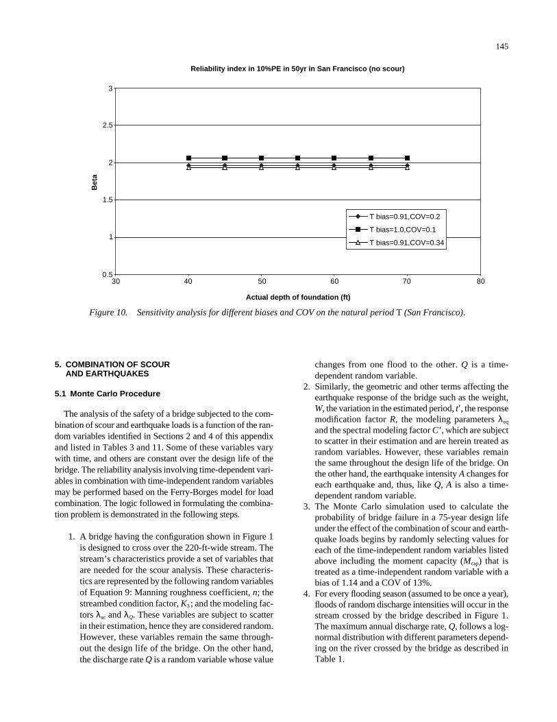
145

5. COMBINATION OF SCOURAND EARTHQUAKES

5.1 Monte Carlo Procedure

The analysis of the safety of a bridge subjected to the com-bination of scour and earthquake loads is a function of the ran-dom variables identified in Sections 2 and 4 of this appendixand listed in Tables 3 and 11. Some of these variables varywith time, and others are constant over the design life of thebridge. The reliability analysis involving time-dependent vari-ables in combination with time-independent random variablesmay be performed based on the Ferry-Borges model for loadcombination. The logic followed in formulating the combina-tion problem is demonstrated in the following steps.

1. A bridge having the configuration shown in Figure 1is designed to cross over the 220-ft-wide stream. Thestream’s characteristics provide a set of variables thatare needed for the scour analysis. These characteris-tics are represented by the following random variablesof Equation 9: Manning roughness coefficient, n; thestreambed condition factor, K3 ; and the modeling fac-tors λsc and λQ. These variables are subject to scatterin their estimation, hence they are considered random.However, these variables remain the same through-out the design life of the bridge. On the other hand,the discharge rate Q is a random variable whose value

changes from one flood to the other. Q is a time-dependent random variable.

2. Similarly, the geometric and other terms affecting theearthquake response of the bridge such as the weight,W, the variation in the estimated period, t′, the responsemodification factor R, the modeling parameters λeq

and the spectral modeling factor C ′, which are subjectto scatter in their estimation and are herein treated asrandom variables. However, these variables remainthe same throughout the design life of the bridge. Onthe other hand, the earthquake intensity A changes foreach earthquake and, thus, like Q, A is also a time-dependent random variable.

3. The Monte Carlo simulation used to calculate theprobability of bridge failure in a 75-year design lifeunder the effect of the combination of scour and earth-quake loads begins by randomly selecting values foreach of the time-independent random variables listedabove including the moment capacity (Mcap) that istreated as a time-independent random variable with abias of 1.14 and a COV of 13%.

4. For every flooding season (assumed to be once a year),floods of random discharge intensities will occur in thestream crossed by the bridge described in Figure 1.The maximum annual discharge rate, Q, follows a log-normal distribution with different parameters depend-ing on the river crossed by the bridge as described inTable 1.

Reliability index in 10%PE in 50yr in San Francisco (no scour)

0.5

1

1.5

2

2.5

3

30 40 50 60 70 80

Actual depth of foundation (ft)

Bet

a

T bias=0.91,COV=0.2

T bias=1.0,COV=0.1

T bias=0.91,COV=0.34

Figure 10. Sensitivity analysis for different biases and COV on the natural period T (San Francisco).

146

5. Given a realization of the random variable Q, the cor-responding flow depth, y0, and velocity, V, are calcu-lated from Equations 7 and 5.

6. For realizations of the modeling factors, λsc and λQ,the roughness factor, n, the bed condition factor, K3,

and the other deterministic parameters, the maximumexpected scour depth for the 1 year, ymax, is calculatedusing Equation 9.

7. Since Q is a time-dependent random variable, then y0

and V are also time-dependent random variables. Con-sequently, the maximum annual scour depth ymax is atime-dependent random variable.

8. The scour depth ymax is assumed to remain constant forthe duration of the flooding season assumed to be 1/2year. During the next flooding season, the value of thescour depth may change depending on the occurrenceof the random variable Q.

9. During the 1/2 year period when ymax exists, there is afinite probability that an earthquake will also occur.

10. The probability distribution for the maximum earth-quake intensity for this 1/2-year period can be obtainedfrom the results of Table 10 by using the relationship

FA(x) = FAlyr(x)1/2 (32)

where A is the maximum earthquake intensity expectedin the 1/2-year period when scour is present, and Alyr isthe maximum earthquake intensity in 1 year as givenin Table 10 for each site considered.

11. Given a realization of the scour depth, ymax obtainedfrom the scour calculations based on the maximumdischarge rate corresponding to 1 year, the effectiveheight of the bridge column becomes

H = 25 ft + ymax + Le (33)

where 25 ft is the original column height, ymax is thescour depth, and Le is the distance between the groundlevel and the point of column fixity. The point of fix-ity is calculated from Equation 10 when the actualdepth of the foundation, L, is adjusted by reducing theoriginal depth by ymax.

12. The change in column height will produce a change inthe stiffness K of Equation 12 and, consequently, willproduce a change in the period of the system. (Thischange would reduce the natural period of the systemand thus reduce the earthquake force, but a higher Hwill also increase the moment arm).

13. On the other hand, the presence of scour will reducethe depth of the foundation by ymax. This in turn willchange the point of fixity of the column Le as shownin Equation 10.

14. For the realizations of the time-dependent variables Aand ymax and all the other time-independent variables,the moment applied on the bridge column is obtainedfrom Equation 30.

15. The moment obtained from Step 14 gives the maxi-mum moment expected to be applied during one flood-ing season due to the possible combination of earth-quake forces and scour.

16. When the flooding season is over, and the scour holeis refilled, an earthquake might still occur and theapplied moment for the earthquake that might hit dur-ing the dry season is calculated in the same mannerdescribed above, but without scour (i.e., with ymax =0.0).

17. The higher of the two moments obtained from the dryseason and the flooding season becomes the maxi-mum yearly moment for the bridge.

18. Since there are 75 years within the design life of thebridge, the process starting with Step 4 is repeated 75times. The maximum moment from all the 75 itera-tions will provide one realization of the maximum 75-year applied moment.

19. Steps 4 through 18 assumed that all the random vari-ables, except for ymax and A, are set at values that werekept fixed over the design life of the bridge. Thesevariables are Manning’s number, n; the scour model-ing factors λQ and λsc ; the stream bed condition factor,K3, as well as the earthquake modeling factor λeq ; thespectral factor, C′; the period, T; the weight, W; andthe response modification factor, R. The means, COVsand probability distributions of these variables that aresampled only once for the bridge design life are givenin Tables 3 and 11. Failure of the bridge is verified bycomparing the maximum 75-year applied moment tothe moment capacity established in Step 3.

20. The Monte Carlo simulation is continued by repeat-ing Steps 3 through 19 by first creating another set ofrealizations for the time-independent random vari-ables, then calculating the maximum 75-year appliedmoment, and checking whether failure will occur. Inthe calculations presented in this appendix, the calcu-lations are repeated a total of 100,000 times. The prob-ability of failure is estimated as the ratio of the num-ber of failures that are counted in Step 19 divided bythe total number of iterations (100,000). The reliabil-ity index, β, is calculated from inverting the followingequation:

Pf = Φ(−β) (34)

where Pf is the probability of failure and Φ is thecumulative normal distribution function.

21. The reliability calculations use the same safety mar-gin given in Equation 31. This safety margin equationconsiders only the failure of the bridge column due tobending moment. Other failure modes such as failurein the soil due to the reduction of the soil depth havealso been considered as will be discussed furtherbelow.

147

5.2 Results for Bending of Bridge Column

The reliability calculations are first executed for the fiveearthquake sites with the discharge data of the CuyahogaRiver. The results illustrated in Figure 11 show that scourdoes not significantly affect the reliability index of the bridgefor the column failure mode because as explained earlier, thepresence of scour reduced the stiffness of the system, but atthe same time increased the moment arm resulting in littlechange in the probability of failure of the column under bend-ing loads. The presence of scour, however, would affectother failure modes, particularly the failure of the soil. Thisphenomenon is explained in Section 5.3.

5.3 Failure of Soil Due to the Combination ofScour and Earthquake Loads

The bridge could fail in different possible modes. Theseinclude moment failure at the base of the columns, shearingfailures along the length of the columns, failure of the soildue to lateral loads, and so forth. The analysis performedabove has shown that the presence of scour did not signifi-cantly affect the safety of the column for failure in bending.In this section, the failure of the foundation due to lateralforces is analyzed.

The model used assumes an equivalent static, linear-elasticbehavior of the soil following Rankine’s method as describedby Poulos and Davis (1980). For the soil conditions of thesite, the internal friction angle of the sand, φ, is equal to 35°.The buoyant unit weight of sand is 60 lb/ft3. The free bodydiagram for the column-foundation-soil system is shown inFigure 12.

In Figure 12, F is the inertial force (equivalent appliedforce), H gives the effective height of the column to the pointof fixity, and Pp is the passive resultant resisting force of thesoil (produced by the triangular soil pressure resisting themotion). According to Poulos and Davis (1980), the activeforce Pp is given as follows:

(34a)

where

γ = the specific weight of sand,L = the depth of the pile;D = the diameter of the pile, andKp = the Rankine coefficient, which is given by

(35)

where φ =35° is the angle of friction for sand.

5.3.1 Definition of Failure

Failure of the soil due to lateral load may occur under twodifferent cases: (1) no hinges form in the column and the soilis unable to resist the applied lateral force on top of the col-umn and (2) a hinge forms in the column at the point of fix-ity and the soil is unable to resist the shearing forces trans-ferred from the hinge. For Case 1, the applied lateral force isobtained from Equation 30a as

Kp = +−

11

sin( )sin( )

φφ

PDK L

pp=

32

2γ

Reliability index 2%PE in 50yr in Cuyahoga (T bias=0.9,COV=0.2)

0.5

1

1.5

2

2.5

3

30 35 40 45 50 55 60 65 70 75

Actual depth of foundation (ft)

Bet

a S.Francisco

Seattle

St. Paul

New York

Memphis

Figure 11. Effect of scour on the reliability index.

148

Pappl = λeq C′ Sa(t′ T) ∗ A ∗ W. (36)

Notice that the response modification factor is not used tocalculate the applied lateral force on the system when nohinges are formed (i.e., when the column remains in the lin-ear elastic range).

For Case 2, the applied force is

(37)

where Mu is the ultimate moment capacity of the column. Theactual ultimate moment capacity is a random variable withstatistics related to the nominal capacity through a bias of1.14 and a COV of 13%, as explained earlier. The safety mar-gin for the failure of the soil is given as

Z = Pp − Fappl (38)

where failure occurs if the safety margin Z is less than 0. Pp

is the lateral force capacity of the soil. The presence of scourwill lower the applied force of Equation 36 because it willreduce the stiffness of the system. Scour would increase themoment arm H, which would also lower the applied force

FMH

uappl =

calculated from Equation 37. On the other hand, scour willdecrease the length of the foundation L, thus reducing thecapacity of the foundation to resist the applied lateral loads.The fact that L is raised to the second power in Equation 34aindicates that the effect of the reduction of L on the founda-tion’s capacity is significant.

Both Pp and Fappl of Equation 38 are random variables. Pou-los and Davis (1980) mention that the bias observed in testresults compared with Equation 34a is on the order of 1.50. Inaddition, the foundation’s capacity to resist lateral load as cal-culated in Equation 34a is a function of the Rankine pressurecoefficient, Kp, the unit weight of sand, γ, and the angle of fric-tion, φ. These are random variables with COVs that mayexceed 20%. In particular, Becker (1996) gives the followingvalues for the COV for the soil parameters: for the unit weightof soil, Vγ = 7%; Vφ = 13% for the angle of friction of sand;and for the Rankine pressure coefficients, VK = 20%. In addi-tion to the uncertainties associated with calculating the Rank-ine coefficients, the difference between the soil resistanceunder static loads and dynamic loads must be considered. Toaccount for the dynamic effects on soils, Bea (1983) proposedto use a cyclic factor with a bias of 1.0 and a COV of 15%. Inaddition to these parameters, which are time-independent ran-dom variables, the foundation strength is a function of thedimension of the foundation. The dimensions are all assumedto be deterministic. The summary of the input data used to cal-culate the reliability of the column foundation to resist lateralload is provided in Table 12.

In addition to the random variables identified in Table 12,the random variables listed in Tables 3 and 11 are used in theMonte Carlo simulation that calculates the reliability of thebridge system subjected to the combination of scour and earth-quake loads. The results for the failure of the soil for the SanFrancisco site are provided in Figure 13.

The results shown in Figure 13 illustrate the importance ofthe foundation depth on the reliability of the bridge systemagainst soil failure due to lateral loads when the bridge is sub-jected to the combination of the scour and earthquake loads.The increase in the reliability index is dramatic because achange in the foundation depth from 50 ft to 60 ft produced achange in the reliability index from 2.14 to 3.05 for the case

F

H

L Pp

Figure 12. Free body diagram of bridgesystem.

TABLE 12 Input data for soil-related random variables

Variable Mean Value COV Distribution Type

Unit weight of soil 60 lb/ft3 7% Normal

Angle of friction 35º 13% Normal

Rankine earth pressure 1.5 nominal value 20% Normal

Cyclic effects 1 15% Normal

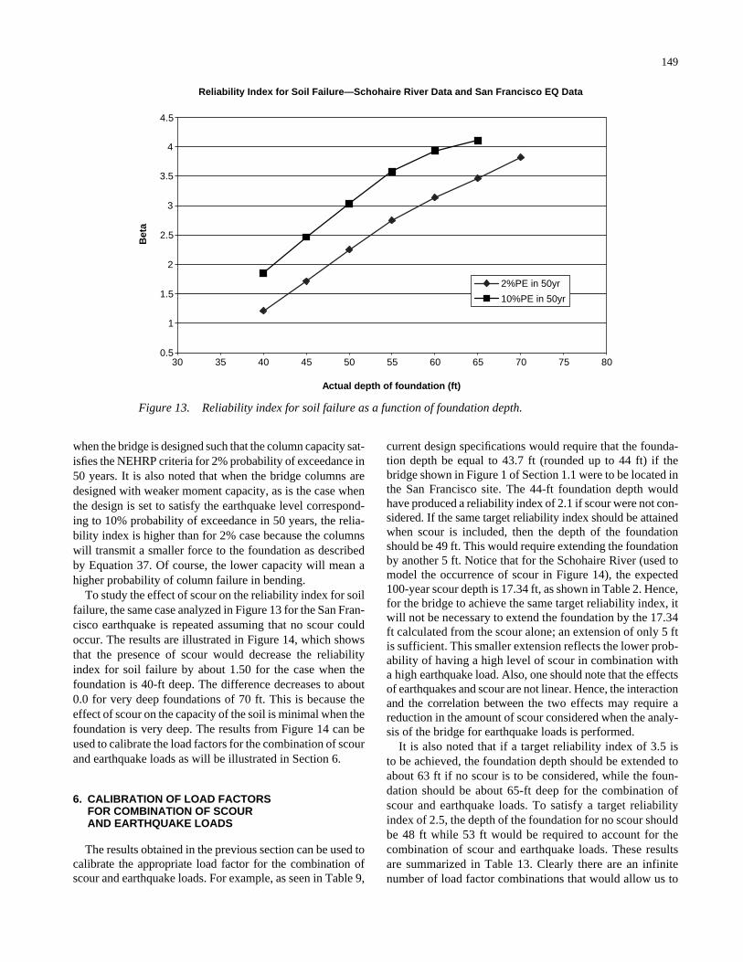
149

when the bridge is designed such that the column capacity sat-isfies the NEHRP criteria for 2% probability of exceedance in50 years. It is also noted that when the bridge columns aredesigned with weaker moment capacity, as is the case whenthe design is set to satisfy the earthquake level correspond-ing to 10% probability of exceedance in 50 years, the relia-bility index is higher than for 2% case because the columnswill transmit a smaller force to the foundation as describedby Equation 37. Of course, the lower capacity will mean ahigher probability of column failure in bending.

To study the effect of scour on the reliability index for soilfailure, the same case analyzed in Figure 13 for the San Fran-cisco earthquake is repeated assuming that no scour couldoccur. The results are illustrated in Figure 14, which showsthat the presence of scour would decrease the reliabilityindex for soil failure by about 1.50 for the case when thefoundation is 40-ft deep. The difference decreases to about0.0 for very deep foundations of 70 ft. This is because theeffect of scour on the capacity of the soil is minimal when thefoundation is very deep. The results from Figure 14 can beused to calibrate the load factors for the combination of scourand earthquake loads as will be illustrated in Section 6.

6. CALIBRATION OF LOAD FACTORSFOR COMBINATION OF SCOURAND EARTHQUAKE LOADS

The results obtained in the previous section can be used tocalibrate the appropriate load factor for the combination ofscour and earthquake loads. For example, as seen in Table 9,

current design specifications would require that the founda-tion depth be equal to 43.7 ft (rounded up to 44 ft) if thebridge shown in Figure 1 of Section 1.1 were to be located inthe San Francisco site. The 44-ft foundation depth wouldhave produced a reliability index of 2.1 if scour were not con-sidered. If the same target reliability index should be attainedwhen scour is included, then the depth of the foundationshould be 49 ft. This would require extending the foundationby another 5 ft. Notice that for the Schohaire River (used tomodel the occurrence of scour in Figure 14), the expected100-year scour depth is 17.34 ft, as shown in Table 2. Hence,for the bridge to achieve the same target reliability index, itwill not be necessary to extend the foundation by the 17.34ft calculated from the scour alone; an extension of only 5 ftis sufficient. This smaller extension reflects the lower prob-ability of having a high level of scour in combination witha high earthquake load. Also, one should note that the effectsof earthquakes and scour are not linear. Hence, the interactionand the correlation between the two effects may require areduction in the amount of scour considered when the analy-sis of the bridge for earthquake loads is performed.

It is also noted that if a target reliability index of 3.5 is to be achieved, the foundation depth should be extended toabout 63 ft if no scour is to be considered, while the foun-dation should be about 65-ft deep for the combination ofscour and earthquake loads. To satisfy a target reliabilityindex of 2.5, the depth of the foundation for no scour shouldbe 48 ft while 53 ft would be required to account for thecombination of scour and earthquake loads. These resultsare summarized in Table 13. Clearly there are an infinitenumber of load factor combinations that would allow us to

Reliability Index for Soil Failure—Schohaire River Data and San Francisco EQ Data

0.5

1

1.5

2

2.5

3

3.5

4

4.5

30 35 40 45 50 55 60 65 70 75 80

Actual depth of foundation (ft)

Bet

a

2%PE in 50yr

10%PE in 50yr

Figure 13. Reliability index for soil failure as a function of foundation depth.

150

design the foundation to achieve the target reliability levelsFor example, to achieve the required foundation depth, oneoption would be to use a load factor on earthquake loadsequal to 1.0 and to increment the foundation depth by afactor of 17.34-ft for design scour depth. For example, bytaking the required 44 ft depth for earthquake alone with0.52 times the design scour depth, a total foundation depthof 53 ft is achieved, leading to a reliability index of 2.5. Thedifferent load factors that may be used on scour to achievedifferent reliability targets are listed in the last column ofTable 13. If a target reliability index of 2.0 is required, thena load factor on scour of 0.23 will be sufficient.

The results summarized in Table 13 are for illustrationonly as the data from the other sites and rivers are still beingsummarized and analyzed. However, it is noted that the dif-ferences from the different sites and rivers are expected to beminimal, as demonstrated in the previous sections, in which

it was observed that the reliability indexes calculated usingthe models described in this report were similar for the dif-ferent site locations and rivers considered.

REFERENCES FOR APPENDIX C

American Association of State Highway and Transportation Officials(1994). AASHTO LRFD Bridge Design Specifications, Washing-ton, DC.

Applied Technology Council (1981). Seismic Design Guidelines forHighway Bridges, ATC-6, Redwood City, CA.

Bea, R.G. (1983). “Characterization of the Reliability of OffshorePiles Subjected to Axial Loadings,” Proceedings of the ASCEStructures Congress, October 1983, TX.

Becker, D.E (1996). “18th Canadian Geotechnical Colloquium:Limit States Design for Foundations, Part II: Development forthe National Building Code of Canada,” Canadian GeotechnicalJournal, Vol. 33; pp. 984–1007.

Reliability Index for Soil Failure—Schohaire River Data and San Francisco EQ Data

1

1.5

2

2.5

3

3.5

4

30 35 40 45 50 55 60 65 70 75

Actual depth of foundation (ft)

Bet

a

2%PE in 50yr(no scour)

2%PE in 50yr

Figure 14. Comparison of reliability index for San Francisco site with scour and without scour.

TABLE 13 Required foundation depth to satisfy different reliability targets

Target reliability

index Depth for no

scour Depth for

scour + EQ

Current EQ design

requirement 1.5 37 ft 43 ft 44 ft

2 43 ft 48 ft 44 ft

2.5 48 ft 53 ft 44 ft

3 55 ft 58 ft 44 ft

3.5 63 ft 65 ft 44 ft

151

Briaud, J.L., Ting, F.C.K., Chen, H.C, Gudavalli, R., Perugu, S.,and Wei, G. (1999). “SRICOS: Prediction of Scour Rate inCohesive Soils at Bridge Piers,” ASCE Journal of Geotechnicaland Environmental Engineering, Vol. 125, No. 4 (April 1999);pp. 237–246.

Chopra, A.K., and Goel, R.K. (2000). “Building Period Formulasfor Estimating Seismic Displacements,” EERI Earthquake Spec-tra, Vol. 16, No. 2.

Ellingwood B., Galambos, T.V., MacGregor, J.G., and Comell,C.A. (1980). Development of a Probability Based Load Criterionfor American National Standard A58, National Bureau of Stan-dards, Washington, DC.

Frankel, A., Harmsen, S., Mueller, C., Barnhard, T., Leyendeker,E.V., Perkins, D., Hanson, S., Dickrnan, N., and Hopper, M.(1997). “USGS National Seismic Hazard Maps: Uniform HazardSpectra, De-aggregation, and Uncertainty,” Proceedings of FHWA/NCEER Workshop on the National Representation of SeismicGround Motion for New and Existing Highway Facilities, NCEERTechnical Report 97-0010, SUNY Buffalo, NY; pp. 39–73.

Haviland, R. (1976). “A Study of Uncertainties in the FundamentalTranslational Periods and Damping Values for Real Buildings,”MIT reports, Cambridge, MA.

Hwang, H.H.M., Ushiba, H., and Shinozuka, M. (1988). “Reliabil-ity Analysis of Code-Designed Structures under Natural Haz-ards,” Report to MCEER, SUNY Buffalo, NY.

Hydraulic Engineering Center (1986). “Accuracy of ComputedWater Surface Profiles,” U.S. Army Corps of Engineers, Davis,CA.

Johnson, P.A. (1995). “Comparison of Pier Scour Equations UsingField Data,” ASCE Journal of Hydraulic Engineering, Vol. 121,No. 8; pp. 626–629.

Landers, M.N., and Mueller, D.S. (1996). “Channel Scour atBridges in the United States,” FHWA-RD-95-l84, Federal High-way Administration, Turner-Fairbank Highway Research Center,McLean, VA.

Liu, W.D., Ghosn, M., Moses, F., and Neuenhoffer, A. (2001).NCHRP Report 458: Redundancy in Highway Bridge Substruc-tures, Transportation Research Board of the National Academies,Washington, DC.

Liu, D., Neuenhoffer, A., Chen, X., and Imbsen, R. (1998). “DraftReport on Derivation of Inelastic Design Spectrum,” Report toNCEER, SUNY Buffalo, NY.

Miranda, E. (1997). “Strength Reduction Factors in Performance-Based Design,” EERC-CUREe Symposium in Honor of VitelmoV. Bertero, Berkeley, CA.

National Earthquake Hazards Reduction Program (1997). Recom-mended Provisions for Seismic Regulations for New Buildingsand Other Structures, Federal Emergency Management Agency,FEMA 302, Building Safety Council, Washington, DC.

Newmark, N.M., and Hall, W.J. (1973). “Seismic Design Criteriafor Nuclear Reactor Facilities,” Building Practices for DisasterMitigation, Report No. 46, National Bureau of Standards, U.S.Department of Commerce; pp. 209–236.

Nowak, A.S. (1999). NCHRP Report 368: Calibration of LRFDBridge Design Code, Transportation Research Board of theNational Academies, Washington, DC.

Poulos, H.G., and Davis, E.H. (1980). Pile Foundation Analysis andDesign, Krieger Publishing Co., FL.

Priestley, M.J.N., and Park, R. (1987). “Strength and Ductility ofConcrete Bridge Columns Under Seismic Loading,” ACI Struc-tural Engineering Journal, January–February.

Richardson, E.V., and Davis, S.R. (1995). Evaluating Scour atBridges, 3rd edition. Report No. FHWA-IP- 90-0 17, HydraulicEngineering Circular No. 18, Federal Highway Administration,Washington, DC.

Seed, H.B., Ugas, C., and Lysmer, J. (1976). “Site-Dependent Spec-tator Earthquake-Resistant Design,” Bulletin of the SeismologicalSociety of America, Vol. 66, No. 1 (February 1976); pp. 221–243.

Shirole, A.M., and Holt, R.C. (1991). “Planning for a ComprehensiveBridge Safety Assurance Program,” Transportation ResearchRecord 1290, Transportation Research Board of the NationalAcademies, Washington, DC; pp. 39–50.

Stewart, J.P., Seed, R.B., and Fenves, G.L. (1999). “Seismic SoilStructure Interaction in Buildings, II: Empirical Findings.” ASCEJournal of Geotechnical and Geoenvironmental Engineering,Vol. 125, No. 1.

Takada, T., Ghosn, M., and Shinozuka, M. (1989). “Response Mod-ification Factors for Buildings and Bridges,” Proceedings fromthe 5th International Conference on Structural Safety and Relia-bility, ICOSSAR 1989, San Francisco; pp. 415–422.

Zahn, F.A., Park, R., and Priestly, M.J.N. (1986). “Design ofReinforced Concrete Bridge Columns for Strength and Ductil-ity,” Report 86- 7, University of Canterbury, Christchurch, NewZealand.

152

APPENDIX H

SEISMIC RISK ANALYSIS OF A MULTISPAN BRIDGE

NCHRP Project 12-49 has recently proposed a set of rec-ommended load resistance factor design (LRFD) guidelinesfor the seismic design of highway bridges, published asNCHRP Report 472: Comprehensive Specifications for theSeismic Design of Bridges (Applied Technology Council[ATC] and the Multidisciplinary Center for Earthquake Engi-neering Research [MCEER], 2002). The proposed LRFDguidelines have adopted and modified many of the featuresoutlined by the existing National Earthquake Hazards Reduc-tion Program specifications (NEHRP, 1997), which were orig-inally intended for buildings, to the design and safety evalua-tion of bridge structures. Thus, for the life safety limit state, theproposed LRFD seismic guidelines use the NEHRP 2,500-year return period earthquake hazard maps along with theresponse spectra proposed by NEHRP, but remove a 2/3reduction factor that is associated with the NEHRP spectralaccelerations. The 2/3 factor had been included by NEHRP toessentially reduce the 2,500-year acceleration spectrum to anequivalent 500-year spectrum for the U.S. West Coast region.

Another major change proposed by NCHRP Project 12-49consists of a new set of response modifications factors thatmore realistically model the nonlinear behavior of bridgecomponents. Specifically, NCHRP Project 12-49 has pro-posed higher response modification factors for multicolumnbents, which would reduce the implicit levels of safety in thedesign process and may offset the use of the more conserva-tive acceleration spectrum. In addition, NCHRP Project 12-49proposed a performance-based design approach wherebydifferent seismic design and analysis procedures (SDAPs)are specified, depending on the seismic hazard level andwhether the bridge is expected to perform adequately for alife safety or operational performance objective (ATC andMCEER, 2002).

The analyses performed in the previous appendixes wereexecuted for bridge piers having foundations formed by pileextensions by modeling the bridge pier as an equivalent sin-gle degree of freedom (SDOF) system after determining theeffective point of fixity. In this appendix, the analysis of anexample bridge founded on a pile system, which had beenpreviously prepared by the NCHRP Project 12-49 team, isreviewed and is used as the basis for the seismic risk analy-sis. This particular analysis is based on a more advanced multi-degree of freedom (MDOF) structural analysis. The objec-tives of this appendix are (1) to compare the results of the riskanalysis obtained using simple SDOF systems with those thatusing an MDOF spectral analysis and (2) to compare thesafety levels of bridge bents founded on multiple piles withthose of bridge bents founded on pile extensions.

1. DESCRIPTION OF EXAMPLE BRIDGE

To achieve the objectives of this appendix, an examplebridge that was used as part of NCHRP Project 12-49 to illus-trate the recommended analysis and design methods isselected for review. Specifically, the bridge selected for thisanalysis is the 500-ft bridge described in the unpublishedDesign Example No. 8 developed under NCHRP Project 12-49. The original site was taken by the NCHRP Project 12-49team to be in the Puget Sound region of Washington state.However, in this appendix, the analysis is repeated for theseismic zone corresponding to Seattle. The change in sitelocation is effected to take advantage of the availability of theSeattle seismic intensity data. The United States GeologicalSurvey (USGS) earthquake hazard maps indicate that, for theSeattle site, the short-period acceleration (0.2 sec) is Ss = 1.61g and the 1.0-sec acceleration is S1 = 0.560 g for the mostcredible earthquake (MCE) corresponding to the earthquakewith a 2,500-year return period.

The 500-ft bridge is formed by five continuous spans of100 ft each. The four monolithic bents are formed by two col-umns, each integrally connected to the cap of the combinedconcrete piles with steel casings that form the foundation sys-tem. The two-column bents are also monolithically connectedto the box girder superstructure through a crossbeam. Expan-sion bearings form the connections between the superstruc-ture and the substructure at the two end stub-type abutments.Figures 1.a, 1.b, and 1.c—which are adopted from the NCHRPProject 12-49 example—provide a description of the bridge.

The NCHRP Project 12-49 team chose to use the com-mercial structural analysis program SAP2000 to perform amultimode spectral analysis of the example bridge. The struc-tural model for each bent is represented by Figure 2, whichis adapted from the unpublished NCHRP Project 12-49 report,in which the effect of the foundation is modeled by a seriesof translation and rotational springs. The same model used inthe NCHRP project report is used in this appendix, whichfocuses on examining the safety of the bridge columns whenthe bridge is subjected to earthquakes having intensities sim-ilar to those expected in Seattle. A separate analysis is exe-cuted for each of the transverse and longitudinal directionsbecause the uncertainties associated with the direction of theearthquake and the use of different possible combination rulesare beyond the scope of this study.

2. ANALYSIS OF EXAMPLE BRIDGE

The bridge example described in the previous section wasanalyzed using the same input data for the structural model

153

Figure 1.a. Plan view of example bridge.

Figure 1.b. Cross section of example bridge.

154

Figure 2.a. Model for structural analysis of example bridge.

Figure 1.c. Profile of bridge example abutment.

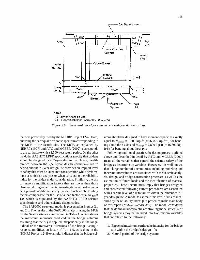
155

that was previously used by the NCHRP Project 12-49 team,but using the earthquake response spectrum corresponding tothe MCE of the Seattle site. The MCE, as explained byNEHRP (1997) and ATC and MCEER (2002), correspondsto the earthquake with a 2,500-year return period. On the otherhand, the AASHTO LRFD specifications specify that bridgesshould be designed for a 75-year design life. Hence, the dif-ference between the 2,500-year design earthquake returnperiod and the 75-year design life provides an implicit levelof safety that must be taken into consideration while perform-ing a seismic risk analysis or when calculating the reliabilityindex for the bridge under consideration. Similarly, the useof response modification factors that are lower than thoseobserved during experimental investigations of bridge mem-bers provide additional safety factors. Such implicit safetyfactors compensate for the use of a load factor equal to γEQ =1.0, which is stipulated by the AASHTO LRFD seismicspecifications and other seismic design codes.

The SAP2000 structural model is presented in Figures 2.aand 2.b. The results of the SAP2000 analysis using the MCEfor the Seattle site are summarized in Table 1, which showsthe maximum moments produced in the bridge columnsassuming that the EQ is applied independently in the longi-tudinal or the transverse directions of the bridge. Using aresponse modification factor of Rm = 6.0, as is done in theNCHRP Project 12-49 example, indicates that the bridge col-

umns should be designed to have moment capacities exactlyequal to Mxdesign = 1,606 kip-ft (= 9638.5 kip-ft/6) for bend-ing about the x axis and Mzdesign = 2,800 kip-ft (= 16,800 kip-ft/6) for bending about the z axis.

Following traditional practice, the design process outlinedabove and described in detail by ATC and MCEER (2002)treats all the variables that control the seismic safety of thebridge as deterministic variables. However, it is well knownthat a large number of uncertainties including modeling andinherent uncertainties are associated with the seismic analy-sis, design, and bridge construction processes, as well as theestimation of future loads and the identification of materialproperties. These uncertainties imply that bridges designedand constructed following current procedures are associatedwith a certain level of risk to failure within their intended 75-year design life. A model to estimate this level of risk as mea-sured by the reliability index, β, is presented in the main bodyof this report (NCHRP Report 489). The model consideredthat the dominant uncertainties controlling the seismic risk ofbridge systems may be included into five random variablesthat are related to the following:

1. Expected maximum earthquake intensity for the bridgesite within the bridge’s design life;

2. Natural period of the bridge system;

Figure 2.b. Structural model for column bent with foundation springs.

156

TABLE 2 Summary of input values for seismic reliability analysis

Variable

Bias

Coefficient of Variation

Distribution Type

Reference

Earthquake modeling, λ eq 1.0 20% Normal Ellingwood et al. (1980)

Spectral modeling, C’ 1.0 Varies per site (15% to 40%)

Normal Frankel et al. (1997)

San Francisco

1.83% g (yearly mean) 333%

Seattle 0.89% g (yearly mean) 415% Memphis 0.17% g (yearly mean) 1707% New York 0.066% g (yearly mean) 2121%

Acceleration A

St. Paul 0.005% g (yearly mean) 3960%

from Figure 3

USGS website

Period, t’ 0.90 20% Normal Chopra and Goel (2000)

Weight, W

1.05 5% Normal Ellingwood et al. (1980)

Response modification, Rm

7.5 (mean value) 34% Normal Priestly and Park (1987); Liu et. al (1998)

Modulus of elasticity, E

1.25 40% Normal Deduced from Chopra and Goel (2000)

Foundation spring stiffness, Ks

1.0 17% Normal Stewart et al. (1999)

3. Spectral accelerations for the site taking into consider-ation the soil properties;

4. Nonlinear behavior of the bridge system; and5. Modeling uncertainties associated with current meth-

ods of analysis.

Information available in the literature about these randomvariables are discussed in detail in the main body of this reportand are summarized in the first six rows of Table 2 of thisappendix. The distribution of the earthquake accelerationsfor different sites are also shown in Figure 3, which is basedon data provided by USGS and Frankel et al. (1997).

As mentioned above, the structural and reliability analysesused in this report are based on an SDOF model of a bridge

bent. The use of a multimodal analysis for this bridge exam-ple implies that the analysis is based on several vibrationmodes. Therefore, the consideration of a single random vari-able, namely t′, to represent the uncertainties associated withdetermining the natural period of the bridge is no longer pos-sible. An alternative approach consists of recognizing thatthe period of the system is a function of the stiffness of thestructural members and those of the foundation. The stiffnessof each member is controlled by the product of the modulusof elasticity and the moment of inertia. If one assumes thatthe moment of inertia is deterministic, then the stiffness ofthe structural member is controlled by one random variable,namely the modulus of elasticity, E. The nominal modulus ofelasticity used in design practice is the value obtained for

TABLE 1 Summary of SAP2000 results for forces and moments in bridgecolumns

Axial Force

(kips) Moment X

(kip-ft) Shear Z

(kip) Moment Z

(kip-ft) Shear X

(kip) EQ Longitudinal Bent 1 column 39 0 0 16,800 1,119 Bent 2 column 56 0 0 7,661 340 Bent 3 column 11 0 0 6,239 249 Bent 4 column 33 0 0 7,688 342 EQ Transverse Bent 1 column 723 7,544 499 1,089 73 Bent 2 column 778 8,028 355 825 37 Bent 3 column 899 9,639 383 295 12 Bent 4 column 790 8,675 383 785 35

concrete at 28 days. However, some researchers have assumedthat the actual long-term modulus for concrete members is onthe order of 1.25 times that of the nominal value. For this rea-son, in the calculations performed in this example, the meanvalue of E is assumed to be 1.25 times the nominal value.This bias will also result in a bias approximately equal to0.90 for the natural period of an SDOF system, which corre-sponds to the period bias used in this report. Using similarlogic, it is proposed to use a coefficient of variation (COV)of VE = 40% for the modulus of elasticity during the reliabil-ity analysis of this bridge example. In fact, VE = 40% wouldresult in a COV of 20% for the period of an SDOF system,which is the same value used during the analyses performedin other appendixes of this report. To account for the uncer-tainties associated with determining the spring stiffness val-ues of the foundation system, the data collected by Stewartet al. (1999) are used. These data indicate that models usedto estimate foundation spring coefficients are associated witha bias equal to 1.0 and a COV on the order of 17%.

This report used a closed-form expression to model theSDOF response of bridge piers to earthquake accelerations.Such a closed-form solution lent itself to the use of full-fledged Monte Carlo simulations to study the risk to failureand calculate the reliability index for a variety of bridge con-figurations. The fact that the response of this bridge example

157

is not based on an explicit formulation but is obtained implic-itly through the use of a commercial analysis program—which requires the interference of the analyst to prepare theinput data and interpret the results—precludes the use of theMonte Carlo simulation that requires an extremely large num-ber of analyses and requires the use of more approximate tech-niques. In particular, the Response Surface Method (RSM) hasbeen used by several researchers to incorporate structuralanalysis results into structural reliability computations. RSM isbased on artificially constructing an equation to model theresponse of the structure using a polynomial fit to the resultsobtained from a limited number of discrete numerical analyses.Melchers (1999) observes that when the approximating surfacefits the point responses reasonably well in the area around themost likely failure point, RSM provides a good estimate of thereliability index, β. Based on these observations and the diffi-culties associated with using a Monte Carlo simulation, RSMis used in this report to obtain estimates of the reliability indexfor the bridge example described above.

The first step in RSM consists of using the structural analy-sis program SAP2000 at various values of the random vari-ables and of studying the response of the bridge for these inputparameters. Melchers (1999) and others (e.g., Ghosn et al.,1994) have indicated that the best points to use during theseanalyses should be selected such that the points lie close to

0.0000001

0.000001

0.00001

0.0001

0.001

0.01

0.1

1

0.001 0.0172 0.103 0.556 2Peak acceleration (g)

Fre

qu

ency

of

exce

edan

ce

New YorkSan FranciscoSeattleSt.PaulMemphis

Figure 3. Annual probability of exceedance curves for peak ground acceleration [based onUSGS website and Frankel et al. (1997)].

158

the most likely failure point. However, since the failure pointis not known a priori, an iterative process must be used. Inthis case, the analysis is first performed at points lying closeto the mean values (mean +/− 1 standard deviation) and addi-tional refinements are introduced following the estimation ofthe location of the most likely failure point. Because the earth-quake intensity is associated with an extremely high stan-dard deviation, the SAP2000 analysis is performed at themean 75-year earthquake acceleration and at points locatedat +/−0.1 times the standard deviation. The results of theSAP2000 analyses are presented in Table 3. Note that theresponse of interest to this example is the maximum bendingmoment in a bridge column. Two cases are considered: (1) theearthquake is applied in the longitudinal direction of the bridgeand (2) the earthquake is applied in the transverse direction ofthe bridge. As mentioned earlier, the two cases are treated sep-arately because the consideration of the earthquake orientationand the directional combination rules are beyond the scope ofthis study.

The results shown in Table 3 demonstrate that the founda-tion stiffness has negligible effect on the maximum momentresponse in the bridge columns. When the earthquake isapplied in the transverse direction, no change is observed inthe maximum bending moment of the columns. If the earth-quake is applied in the longitudinal direction, a change ofonly 1.7% is observed when the change in the foundationstiffness is equal to 34% (2 times the standard deviationsaround the mean value). Changes of +/−1 standard deviationin the weight of the structure result in a change of less than5% in the maximum bending moment. On the other hand,changes between 40% and 50% in the bending moments areobserved when the spectral accelerations and the modulus ofelasticity are changed by +/−1 standard deviation each. Achange in the expected 75-year earthquake peak ground accel-eration (PGA) by +/−0.10 standard deviation results in achange of about 13% in the columns’ maximum bendingmoment. When the information summarized in Table 3 is used

in a first order Taylor series expansion, the response surfacemay be represented by an equation of the following form:

Manalysis transverse = −6,409 + 12,523 EQ + 0.002879 E+ 3,790 C′+ 9,735 bW + 0 bKs

(1)

and

Manalysis long = −11,765 + 23,322 EQ + 0.00568 E+ 6,900 C′ + 17,090 bW + 0 bKs

(1′)

where

Manalysis transverse and Manalysis long = the maximum momentresponse due to earthquakes in the transverseand longitudinal directions, respectively;

EQ = the earthquake PGA;E = the modulus of elasticity;C′= the modeling variable of the spectral acceler-

ation; andbW and bKs = factors that multiply the weights, W, and the

foundation stiffness, Ks, respectively.

The normalized factors, bW and bKs, are used because eachbridge element may have a different weight, and each foun-dation stiffness my be different. The normalized factors bW

and bKs in Equations 1 and 1′ express how the final momentchanges when all the individual weights and stiffnesses arevaried by the same factor. When the mean values of theweights are used, bw is set at 1.0. Similarly, when the mean val-ues of Ks are used, bKs is set at 1.0. The model assumes that allthe element weights are correlated such that a change of theweight of one element by a certain factor leads to the multi-plication of all the other elements’ weights by the same factor.A similar assumption is made for the foundation stiffnesses.

The results shown in Table 1 indicate that the design proce-dure proposed in NCHRP Project 12-49 [ATC and MCEER,

TABLE 3 Results of parametric analysis close to mean values

EQ Transverse EQ Longitudinal

Moment about x

(kip-ft)Moment about z

(kip-ft) Base case = analysis at mean values 3,879 6,900 75-yr EQ + 0.1 σ EQ 4,054 7,251 75-yr EQ – 0.1 σ EQ 3,560 6,331 C’ + σ C’ 4,849 8,626 C’– σ C’ 2,954 5,176 W + σW 3,970 7,057 W – σW 3,786 6,734 E +σE 4,595 8,289 E – σE 3,006 5,153 Ks + σks 3,879 6,841 Ks σ– ks 3,879 6,960

159

2002) would dictate that the columns be designed to havemaximum capacities Mcap transverse = Mdesign transverse = 1,606 kip-ft(9,638.5 kip-ft/Rm) where the 9,638.5 kip-ft is the momentobtained by analyzing the structure under the effect of the2,500-year earthquake and the nominal values of the materialproperties and spectral accelerations, and Rm nominal = 6.0 is thenominal response modification factor specified by NCHRPProject 12-49 for multicolumn bents. For the longitudinal direc-tion, the required moment capacity is Mcap long = Mdesign long =2,800 kip-ft.

Failure occurs when the applied moment is higher than orequal to the design moment. The applied moment obtainedfrom the SAP2000 analysis does not account for the nonlin-ear response that is normally represented using a responsemodification factor, Rm. In addition, to account for the mod-eling uncertainties, Ellingwood et al. (1980) have suggestedthat a modeling factor λEQ must also be included in the relia-bility analysis. This would lead to a failure function, Z, thatcan be represented by the equation

Z = Mcap – λEQ Manalysis /Rm (2)

where Mcap is a random variable that, according to Nowak(1999), follows a lognormal distribution with a bias equal to1.14 and a COV of 13%. The modeling factors λEQ and Rm

are also random variables having the properties described inTable 2 above, and Manalysis is a function of the random vari-ables EQ, C′, E, W, and Ks (or, more precisely, bW and bKS).In the first iteration, the function that gives Manalysis is describedin Equation 1 when the bridge is subjected to earthquakes inthe transverse direction and in Equation 1′ when the bridgeis subjected to earthquakes in the longitudinal direction. MonteCarlo simulations using Equations 1 or 1′ with Equation 2produced reliability index values of β = 1.76 for the trans-verse direction and β = 1.73 for the longitudinal direction.Through the review of the various cases that fall within the

failure region, the Monte Carlo simulation also indicates thatthe most likely failure point occurs when EQ* = 0.56g, E* =1.36En (bW* = 1.05) or W* = Wn, bC ′* = 1.07 and when bKs* =1.0 or K s* = Ksn for the earthquake in the transverse direc-tion. The maximum likely failure point occurs when EQ* =0.60g, E* = 1.39En, W* = 1.05Wn, C′* = 1.08, and Ks* = Ksn

when the earthquake is applied in the longitudinal direction.These most likely failure points are then used to perform a sec-ond iteration of the parametric analysis with results describedin Table 4. These will in turn lead to new sets of response func-tions similar but with slightly different coefficients than thosein Equations 1 and 1′.

The use of the results presented in Table 4 along withEquation 2 within a second and third reliability analysis leadsto an updated reliability index of β = 1.76 for the transversedirection and 1.74 for the longitudinal direction. The analy-sis is then repeated for various values of Mcap and is illustratedin Figure 4.

TABLE 4 Results of parametric analysis close to most likelyfailure point

EQ Longitudinal EQ Transverse

RM = 6 Moment about z

(kip-ft) Moment about x

(kip-ft) Base case = most likely failure point 18,851 10,722 EQ* + 0.1 σEQ 19,352 10,986 EQ* – 0.1 σEQ 18,351 10,444 C’* + 0.2 σC’ 19,714 11,216 C’* – 0.2 σC’ 17,987 10,228 W* + 0.2 σW 18,948 10,772 W* – 0.2 σW 18,752 10,658 E* + 0.2 σE 19,566 11,097 E* – 0.2 σE 18,116 10,311 Ks* + 0.2 σks 18,814 10,722 Ks* –0.2 σks 18,887 10,722

Reliability Index versus Moment Capacity

0

0.5

1

1.5

2

2.5

3

0 0.5 1 1.5 2 2.5

Mcap/Mdesign

Bet

a

Tranverse

Longitudinal

Figure 4. Variation of reliability index versus moment capacity.

160

The results of Figure 4 show that the reliability index val-ues for the longitudinal and transverse directions produce areliability index on the order of 1.75 if the proposed designguidelines of NCHRP Project 12-49 were to be adopted(Mcap/Mdesign = 1.0) (ATC and MCEER, 2002). The reliabil-ity index would increase to close to 2.35 when the momentcapacity of the columns is selected to have capacities equalto twice the recommended design capacities (Mcap/Mdesign =2.0). This increase in the reliability index could then beachieved by, for example, requiring the use of a responsemodification factor during the design process of Rm = 3.0 ratherthan the Rm = 6.0 that has been recommended by NCHRPProject 12-49. It is to be noted that because the analysisaccounted for the nonlinear behavior of the members, the cal-culations executed herein correspond to the reliability of thebridge system. The reader is reminded that reliability indexon the order of β = 3.5 has been used as the basis for thedesign of bridge members under gravity loads. The presenceof system redundancy would increase the system reliabilityindex under gravity to β > 4.0. The lower reliability indexvalues for earthquake loads is justified in the engineeringcommunity on the basis of an informal cost-benefit analysiswhereby expert chief bridge engineers contend that there isgeneral satisfaction with current design procedures giventhe excessive economic costs that would be associated withincreasing the current reliability levels.

The results in Figure 4 show that the reliability index val-ues are lower than those calculated in the main body of thisreport (NCHRP Report 489). This observed difference is dueto the fact that the analysis performed herein is for the bridgecolumns while the analysis in the main body of the report wasfor the extension pile in the bridge foundation. The differ-ence is primarily caused by the use of a lower response mod-ification factor of Rm = 1.5 for the extension pile as opposedto the Rm = 6.0 used herein for bridge columns supported onmulti-pile foundations.

To study the effect of the nominal value of the responsemodification factor Rm used for design on the reliability index,the reliability analysis of this five-span bridge is repeated fordifferent values of the response modification factor and com-pared with the three-span bridge example analyzed in themain body of the report. The results for the case in which theearthquake is applied in the transverse direction are com-pared in Figure 5.

The results shown in Figure 5 demonstrate how the relia-bility index increases with the use of higher response modi-fication factors and how the results obtained from this exam-ple based on an MDOF SAP2000 analysis of a multispanbridge founded on multi-pile foundation systems approach theresults obtained in the body of the report for bridges on exten-sion piles analyzed as SDOF systems. It is clear from theresults that the major difference is due to the use of differentresponse modification factors for different bridge members.

3. CONCLUSIONS

This appendix executed a reliability analysis for the seis-mic response of a five-span bridge with columns supported onmulti-pile foundations and compared the results with thoseobtained in other parts of this report for bridges analyzed asSDOF systems. The results illustrate the following points:

1. The simplified analysis using an SDOF system yieldsresults consistent with those obtained from the moreadvanced multimodal structural analysis.

2. RSM yields reasonable approximations to the reliabil-ity index for the seismic risk analysis of simple bridgeconfigurations.

3. The use of a response modification factor of Rm = 6.0 forbridge columns associated with the 2,500-year NEHRPspectrum produces system reliability index values onthe order of 1.75. This is much lower than the member

Effect of response modification factor

0

0.5

1

1.5

2

2.5

3

3.5

0 0.5 1 1.5 2 2.5

Mcap/Mdesign

Bet

a

NCHRP 12-48

Rm=1.5

Rm=4

Rm=6

Figure 5. Effect of response modification factor on reliability index.

161

reliability equal to 3.5 used as the basis for calibratingthe LRFD code for members under gravity load.

4. Large differences in the reliability indexes are observedfor the different components of bridge subsystems sub-jected to seismic events. For example, the foundationsystems produce much higher reliability index valuesthan do the bridge columns. This difference has beenintentionally built into the bridge seismic design processby the code writers (i.e., the NCHRP Project 12-49research team) in order to account for the consequencesof the failure of different members. However, the dif-ference is rather large, producing a beta that varies froma value of about β = 3.0 when a response modificationfactor equal to Rm = 1.0 is used to about β = 1.75 whena response modification factor of Rm = 6.0 is used dur-ing the design process. It is noted that the use of aresponse modification factor of Rm = 1.0 implies a designbased on the elastic behavior of members while an Rm =6.0 accounts for the plastic behavior of bridge columns.

5. Although not common in the realm of seismic bridgeengineering, the use of the reliability index as a mea-sure of bridge safety for all types of extreme events willprovide a consistent measure that will help in calibrat-ing load combination factors as executed during thecourse of this study (see Chapter 3 of this report).

REFERENCES FOR APPENDIX H

Applied Technology Council and the Multidisciplinary Center forEarthquake Engineering Research (2002). NCHRP Report 472:Comprehensive Specification for the Seismic Design of Bridges,Transportation Research Board of the National Academies,Washington, DC.

Chopra, A.K., and Goel, R.K. (2000). “Building Period Formulasfor Estimating Seismic Displacements,” EERI Earthquake Spec-tra, Vol. 16, No. 2.

Ellingwood B., Galambos, T.V., MacGregor, J.G., and Comell,C.A. (1980). Development of a Probability Based Load Criterionfor American National Standard A58, National Bureau of Stan-dards, Washington, DC.

Frankel, A., Harmsen, S., Mueller, C., Barnhard, T., Leyendeker,E.V., Perkins, D., Hanson, S., Dickrnan, N., and Hopper, M.(1997). “USGS National Seismic Hazard Maps: Uniform HazardSpectra, De-aggregation, and Uncertainty,” Proceedings of FHWA/NCEER Workshop on the National Representation of SeismicGround Motion for New and Existing Highway Facilities, NCEERTechnical Report 97-0010, SUNY Buffalo, NY; pp. 39–73.

Ghosn, M., Moses, F., and Khedekar, N. (1994). “Response Func-tion and System Reliability of Bridges,”Probabilistic StructuralMechanics: Advances in Structural Reliability Methods; Springer-Verlag; pp. 220–236.

Liu, D., Neuenhoffer, A., Chen, X., and Imbsen, R. (1998). “DraftReport on Derivation of Inelastic Design Spectrum,” Report toNCEER, SUNY Buffalo, NY.

Melchers, R.E. (1999). Structural Reliability: Analysis and Predic-tion, John Wiley & Sons, New York, NY.

National Earthquake Hazards Reduction Program (1997). Recom-mended Provisions for Seismic Regulations for New Buildingsand Other Structures, Federal Emergency Management Agency,FEMA 302, Building Safety Council, Washington, DC.

Nowak, A.S. (1999). NCHRP Report 368: Calibration of LRFDBridge Design Code, Transportation Research Board of theNational Academies, Washington, DC.

Priestley, M.J.N., and Park, R. (1987). “Strength and Ductility ofConcrete Bridge Columns Under Seismic Loading,” ACI Struc-tural Engineering Journal, January–February.

Stewart, J.P., Seed, R.B., and Fenves, G.L. (1999). “Seismic SoilStructure Interaction in Buildings, II: Empirical Findings.” ASCEJournal of Geotechnical and Geoenvironmental Engineering,Vol. 125, No. 1.

162

APPENDIX I

ANALYSIS OF SCOUR DATA AND MODIFIED RELIABILITY MODEL FOR SCOUR

1. INTRODUCTION

The AASHTO LRFD specifications (1998) state that “amajority of bridges that have failed in the United States andelsewhere have failed due to scour.” This is confirmed byShirole and Holt (1991), who observed that over the last 30years, more than 1,000 of the 600,000 U.S. bridges havefailed and that 60% of these failures are due to scour whileearthquakes accounted for only 2%. Of course, there are manymore bridges that are posted or otherwise taken out of servicedue to their inadequate strengths (e.g., due to deterioration,low rating, fatigue damage, etc.); nevertheless, scour is con-sidered a critical cause of failure because its occurrence oftenleads to catastrophic collapses. For this reason, developingmethods for the design and maintenance of bridge founda-tions subjected to risk from scour as well as developing toolsto detect the presence of scour are currently considered toppriorities for agencies concerned with the safety of bridges.

Scour is typically assessed using the methodologies pre-sented in FHWA’s Hydraulic Engineering Circular No. 18(Richardson and Davis, 1995), known as “HEC-18.” Althoughthe HEC-18 model requires designing bridges to sustainfoundation scour associated with the water flow depth andvelocity corresponding to the 100-year or overtopping floodevent, the remaining variables in the HEC-18 equations areconsidered to be deterministic. In other words, once the 100-year water depth and flow velocity have been estimated, theHEC-18 methodology, like most typical design procedures,uses a deterministic design approach with safety factors thatimplicitly account for uncertainties in the models, the pa-rameters, or the hydraulic and hydrologic variables. TheHEC-18 design equation for scour depth around bridge piersis given as follows:

(1)

where

ys design = the nominal or design scour depth;y1 = the upstream flow depth;D = the effective pier width;F0 = Froude number; and

K1, K2, K3 and K4 are correction factors for the pier shape,angle of attack, bed forms, and sediment grada-tion, respectively.

The flow depth, y1, and the flow velocity used to calculate theFroude number are those corresponding to the 100-year orovertopping flood. The safety factors may be included in the

yy

K K K K Dy

Fsdesign

11 2 3 4

1

0 65

00 432 0=

.

..

bias factor of 2.0, the correction factors, Ki , and/or the usageof 100-year return period for y1, which is longer than the 75-year design period stipulated for the design of bridges underthe LRFD specifications.

If Equation 1 is developed to provide a safe (or nominal)value for scour depth, the actual depth of scour, ys scour, maybe obtained from the following:

(2)

where λ is a modeling factor which has an average valueequal to 0.55 as reported by Johnson in Appendix B of thisreport.

If a bridge foundation is designed to satisfy Equation 1 andthe actual depth of scour is obtained from Equation 2, themargin of safety, Z, can be defined as follows:

Z = ys design − ys actual. (3)

Failure would occur when ys actual is greater or equal to ys design

or when the margin of safety, Z, is less than or equal to zero.Once the designer chooses the parameters of Equation 1 fol-lowing the HEC-18 guidelines, ysdesign will be exactly known.On the other hand, because of the randomness in the scourprocess, the determination of the actual scour depth ys actual isassociated with large uncertainties, and ys actual must be con-sidered to be a random variable. The sources of randomnessare primarily due to the following.

• The modeling uncertainties associated with the HEC-18equation, which does not provide very accurate estimatesof scour depths even if all the input data are preciselyknown.

• The uncertainties associated with predicting the inputdata. These, as identified by Johnson (see Appendix B),are primarily due to the following:– The determination of the maximum 75-year discharge

rate.– The determination of the flow depth and flow velocity

corresponding to the 75-year discharge rate. Becausefor known channel profiles the flow and flow veloc-ity are obtained from the discharge data based onManning’s roughness coefficient, the uncertainties areassumed to be primarily due to the determination ofthe appropriate Manning coefficient to use.

– The random variation in river bed conditions and itsinfluence on scour depth as represented by the factorK3 in the above equations.

yy

K K K K Dy

Fsactual

11 2 3 4

1

0 65

00 432 0=

.

..λ

163

The prediction of the 75-year probability of failure, Pf , isdefined as the probability that Z ≤ 0 and can be estimatedbased on the statistical data describing the randomness of eachof the variables that affect Equation 3, as described above andas listed in Table 1.

Although safety factors (or biases) may have been intro-duced into the empirically derived HEC-18 models, there isalways a finite chance that the actual scour depth is largerthan the design scour depth. This is due to the uncertaintiesassociated with predicting the maximum flow depth and veloc-ity that the river will be exposed to within the bridge’s designperiod and the uncertainties associated with determining thecorrection factors, Ki, as well as the modeling errors that areintroduced by the HEC-18 equations. The object of this appen-dix is to provide an explicit accounting for the uncertaintiesand the implied risks of the current scour design methodol-ogy in order to verify the compatibility between the safetyof bridges subjected to scour and other loads and extremeevents. To address issues related to structural risk, recentdevelopments in bridge design procedures have used areliability-based methodology to calibrate load and resis-tance safety factors. The goal of the calibration is to providea consistent level of risk for the range of pertinent bridgegeometries and loading conditions. The nominal measure ofrisk that is used during the calibration process is the reliabil-ity index, β, that is mathematically related to the probabilityof failure, Pf , by

β = Φ−1(Pf) (4)

where Φ−1 is the inverse function of the cumulative normaldistribution.

The reliability index, β, would give an exact measure ofrisk if all the random variables that affect the safety of thebridge component under consideration are properly identifiedalong with their probability distribution types and pertinentstatistics. Because of the difficulty of calculating Pf exactly,in most practical situations, the reliability index is calculatedusing approximate methods such as first or second order reli-ability method (FORM or SORM) algorithms or Monte Carlo

simulations. Also, because many of the random variables thatcontrol the probability of failure are difficult to identify, cat-egorize, and estimate and also because the statistical databasefor civil engineering applications is usually very limited, thereliability calculations would provide only a nominal measureof risk rather than an actuarial value. These limitations pro-duce what is generally known as “modeling uncertainties.”

To reduce the effects of the above-mentioned modelinguncertainties, the calibration of new design codes is often exe-cuted to match the reliability index obtained from existing“satisfactory” designs rather than satisfying a predeterminedspecific value for the probability of failure. This approach hasworked reasonably well when calibrating load and resistancefactors for bridges having typical geometries and materialshaving a long history of satisfactory performance under rea-sonably predictable loading conditions and when the reliabil-ity index, β, has been used as the primary criterion for devel-oping new design codes. Analyses performed during thecourse of this study have demonstrated that the reliabilityindex is highly controlled by the statistical properties of themodeling variable λ. For this reason, this appendix will focuson studying the modeling uncertainties associated with thescour design procedures and the influence of these uncer-tainties on the estimates of the reliability index. This analy-sis is based on the data provided by Landers and Mueller(1996) in their study supported by the FHWA.

2. SCOUR MODELING UNCERTAINTIES

For the reliability analysis of bridge piers subjected toscour, a Monte Carlo simulation can be used to generate ran-dom samples for each of the random variables that control thesafety margin Z of Equation 3 based on their specified proba-bility distributions. The estimation of the statistics includingmean values and coefficients of variation (COVs) of the per-tinent variables as well as the probability distribution typesdepend on each bridge’s pier geometry, channel configura-tion, and channel bed properties. Evidently, several difficul-ties arise when attempting to estimate the properties of the

TABLE 1 Input data for reliability analysis for scour alone

Variable Mean Value

Coefficient of Variation

Distribution Type

Reference

Q, discharge rate

From Table 2.8 From Table 2.8 Lognormal Based on USGS website

λQ, modeling variable for Q

1.0 5% Normal Based on USGS website

λsc, modeling variable 0.55 52% Normal Johnson (1995)

n, Manning roughness 0.025 28% Lognormal Hydraulic Engineering Center (1986)

K3, bed condition factor 1.1 5% Normal Johnson (1995)

164

variables that control scour at specific bridge sites, particu-larly when the bridge has not yet been constructed and actualmeasurements on the maximum scour depth are not available,even over limited periods of time. Even when such measure-ments may be available, the projection of the expected scourdepth over the full design life of the bridge is associated withlarge levels of uncertainty. Added to these difficulties is therealization that the HEC-18 equations were primarily devel-oped based on a limited number of small-scale laboratoryexperiments under “ideal” flow conditions and uniform sandbed materials that may not resemble actual field conditions.In fact, several investigations have shown large discrepan-cies between observed scour depths and those predicted fromthe HEC-18 equations. Because of all the limitations of theHEC-18 model, a procedure that takes into consideration themodeling uncertainties in an explicit manner while studyingthe safety of bridges subjected to scour is initiated in thisappendix.

In assessing the safety of bridge piers subjected to scour,four broad sources of uncertainty are relevant: (1) inherentvariability, (2) estimation error, (3) model imperfection, and(4) human error. Inherent variability, often called “random-ness,” may exist in the characteristic of the bridge structureor in the environment to which the structure is exposed.Inherent variability is intrinsic to nature and is beyond thecontrol of the engineer or code writers. The uncertainties dueto estimation error and model imperfection are extrinsic and,to some extent, reducible. For example, a reliability analystmay choose to obtain additional information to improve theaccuracy of estimation. The uncertainty due to human errormay also be reduced by implementing rigorous quality-controlmeasures during the collection, interpretation, and analysisof scour data. Such improvements, however, usually entailan investment in time and money that the analyst may not bewilling to undertake. In addition, this effort requires the capa-bility of collecting such data at the site of interest. During thebridge design process when the bridge is still in the planningstages, the collection of site-specific data is not possible.Hence, it is usual to rely on design models developed basedon data from other sites and for different bridge configura-tions and to project these available data to the particular siteand bridge conditions. Hence, improving the quality of thedata collection effort is not a viable option during the designstages, although this can be achieved at later stages whenchecking the safety of existing bridges. This study focuses ondeveloping load factors for the design of new bridges underextreme events. Thus, the study must rely on available datacollected from a variety of sites under different conditions toobtain estimates of the modeling uncertainties that describethe relationship between the expected scour depths and thosepredicted from the HEC-18 equations. In bridge engineeringpractice, pier scour depth is estimated using the HEC-18model with Equation 1.

Field observations have shown that even when all the per-tinent parameters of HEC-18 are known, large discrepanciesstill exist between the measured scour depths and those of theHEC-18 equations. These differences are attributed to theuncertainties in the HEC-18 model. To account for thesemodeling uncertainties, Equation1 can be modified by insert-ing a model correction factor, λ, which is defined as follows:

(5)

so that the actual depth of scour, ys actual, may be obtainedfrom Equation 2. Notice that λ as defined in Equation 5 pro-vides an inverse measure of safety such that a lower value ofλ implies a higher level of safety. Also, since λ is a randomvariable, the higher its COV is, the higher the probability isthat the actual depth of scour will exceed the design valueand, hence, the lower the safety of the system is.

The mean value of λ is defined as λ and its standard devi-ation as σλ. These can be estimated from observations ofscour depths at bridge piers and by comparing the observedscour depths with those predicted using the HEC-18 equa-tion. For example, a 1996 study supported by FHWA has col-lected an extensive set of data on observed scour depths andcompared these with different prediction models includingthe HEC-18 equations. The data published in the report byLanders and Mueller (1996) provides ys actual and sufficientinformation to calculate ys design for different sites, channelbed materials, and types of bridge piers. Table 2 provides asummary of the average values of λ and its COV for severaldifferent categories and groupings of the data.

A total number of 374 local scour measurements at differ-ent bridge piers were assembled from the report of Landersand Mueller (1996). Of these measurements, 240 were col-lected in channels with live-bed conditions and the rest werefor piers set in clear-water conditions. Live-bed conditionsoccur when the water channel carries soil particles that aredeposited on the channel floor at low flow speeds. Thesedeposits would refill the scour hole such that under live-bedconditions, the scour process becomes cyclical. From Table2, it is observed that the COV for the data collected in live-bed channels is lower than that obtained from all the data.Out of the 240 measurements taken in live-bed channels, 126were for piers with rounded noses, 52 of the piers had squarenoses, 30 piers were cylindrical, and 32 had sharp noses. Onthe other hand, 191 of the bridges had single-pier bents and49 had pier groups. The bridge piers were also classifiedbased on three types of foundations: (1) piles, (2) poured, and(3) unknown. The soil type is classified as noncohesive soilor unknown soil. Only 18 data points satisfied the conditionsof cylindrical single poured piers in live-bed channels hav-ing noncohesive soils. When all the data are analyzed simul-taneously, the COV is 64.6%, indicating a very high level ofmodeling uncertainties. Large differences in the mean values

λ =yys

sactual

design

165

and/or COVs are observed for different pier shapes, founda-tion types, and so forth. Lower COVs are observed when thedata are categorized based on pier shape and streambed con-ditions. As an example, the mean value of λ for the 18 casesthat have cylindrical poured piers in noncohesive soils wasfound to be 0.36 with a COV of 37.1%. The piers withrounded noses produced a mean value of λ equal to 0.41 witha COV equal to 44.6%. The lowest value of COV is observedfor the case of cylindrical piers in poured foundations set inlive-bed channels with noncohesive soils. Presumably, thislower COV of 37.1% reflects the fact that the HEC-18 modelwas primarily developed based on laboratory simulationsunder these same conditions. Although the lowest in Table 2,a COV of 37.1% still indicates a high spread in the observeddata away from the mean value. The bias of 0.36 for this caseimplies a conservative design equation with an implicitsafety factor on the order of 2.82 (1/0.36).

The point estimates of the mean and the standard devia-tions of λ given in Table 2 are obtained from a limited set ofdata. To convey information on the degree of accuracy ofthese estimates, one should recognize that λ is a random vari-able with (unknown) mean µλ and with (unknown) standarddeviation σλ. The sample means that values of λ given inTable 2 are estimates of µλ for various data sets. The precisionof these estimates can be assessed using the fact that a samplemean λ is a random variable with mean value equal to µλ anda standard deviation of where n is the samplesize. It is noted that for large sample sizes, λ will approach anormal distribution, and the confidence intervals for λ may beobtained using the normal probability tables. The data ofLanders and Mueller (1996) also provide estimates of σλ

(column 4 standard deviation) from which σλ is calculated asgiven in the last column of Table 2. Notice how, in manyinstances, as the classification of the data is narrowed to spe-

σ σλ λ= ( ) /2 n

cific categories of pier shapes and water channel conditions,the standard deviation (σλ) decreases; however, since thenumber of samples used to calculate λ decreases also, thestandard deviation of λ (i.e., σλ) increases, thus expressing alower level of precision in the estimation of λ.

The data from all 374 cases are plotted in a histogram, asis shown in Figure 1. The figure also shows the histogramsthat would be obtained if the data were assumed to follow anormal distribution or a lognormal distribution. The plotsseem to indicate that the modeling variable λ may be rea-sonably well modeled by a lognormal distribution. Furtherverification of this observation for different subsets of thedata is undertaken below.

The data from the live-bed channels consisting of 240 datapoints are also plotted using a lognormal probability scale, asis shown in Figure 2. The plot further verifies that λ for this setof data may be reasonably well represented by a lognormaldistribution. Other probability plots for different sets of dataare provided in Figures 3, 4, and 5. In particular, Figure 3 plotsthe modeling factor λ for rounded poured piers set in live-bedchannels with noncohesive soils on a normal probability curve.Figure 4 plots the same data on a lognormal probability scale.Figure 5 gives a plot on a lognormal scale for the data assem-bled for cylindrical poured piers in live bed-channels with non-cohesive soils. It is noted that Figures 3 and 4 show that thedistribution of λ for the rounded piers approaches a normaldistribution near the upper part of the curve (i.e., for high val-ues of λ) while for low values of λ, the probability distribu-tion more closely approaches that of a lognormal distribu-tion. On the other hand, a lognormal distribution seems to beappropriate for the cylindrical piers, as shown in Figure 5.

The chi-squared goodness-of-fit tests for the data sets plot-ted in Figures 2 through 5 were executed as summarized inTables 3 through 6. The results confirm the observations made

TABLE 2 Summary of mean and COV of based on data of Landers and Mueller (1996)

Flow and channel material

type Pier

shape Mean Standard deviation COV

Number of

observations

Standard deviation of mean

All cases 0.412 0.266 0.646 374 0.0138

Channels with live-bed conditions only 0.429 0.247 0.576 240 0.0159

Rounded 0.400 0.231 0.577 126 0.0206

Sharp 0.523 0.292 0.558 32 0.0516

Cylinder 0.383 0.204 0.532 30 0.0372 All channel bed material Square 0.432 0.246 0.570 52 0.0341

Noncohesive soils All shapes 0.417 0.237 0.569 195 0.0170

Unknown soil type All shapes 0.479 0.283 0.593 45 0.0422

Single piers All shapes 0.405 0.223 0.550 191 0.0161

Pier groups All shapes 0.535 0.310 0.580 49 0.0443

Pile foundation All shapes 0.421 0.256 0.607 158 0.0204

Poured foundation All shapes 0.419 0.185 0.442 67 0.0226

Unknown foundation All shapes 0.547 0.361 0.660 15 0.0932

Noncohesive soils, poured Rounded 0.405 0.181 0.446 48 0.0261

Noncohesive soils, poured Cylinder 0.355 0.132 0.371 18 0.0311

166

from the probability plots. In particular, the chi-squared testfor the complete data as depicted in Table 3 shows that thedata are not inconsistent with the assumption that the under-lying distribution is lognormal with a significance level of5%. In fact, the sum of the squared difference between theobserved frequencies and the corresponding lognormal fre-quencies divided by the lognormal frequency produced a sumequal to 1.02, which is lower than the value of the appropriateχ f

2 distribution at the cumulative probability of 95%, which isgiven in probability tables as C1 − α, f = 7.81 where α = 5% andf = 3. On the other hand, the assumption of a normal distribu-

tion produces a sum of the squared difference equal to 45.86,which is much higher than C1 − α, f = 7.81. Table 4 shows thesame results for the data set consisting of 240 samples col-lected at sites with live-bed conditions. Table 5 gives theresults for the scour-modeling ratio, λ, for the 48 roundedpoured piers set in noncohesive soils in live-bed channels.Table 6 gives the same analysis for the cylindrical piers. It isnoted that for all the cases considered, the lognormal distri-bution is acceptable within the 5% confidence level. How-ever, Table 5 shows that for the rounded piers, the normaldistribution would also be valid.

Comparison of actual data with assumed distribution

0

20

40

60

80

100

120

140

160

<0.2 0.2-4.0 0.4-0.6 0.6-0.8 0.8-1.0 >1.0

Interval

Fre

qu

ency

nu

mb

er

Number of Normal Distribution

Actual Number

Number of Log-NornalDistribution

Figure 1. Histogram for distribution of λ.

Log-normal probability paper

Cumulative Probability

1 10 30 50 70 90 99

Rat

io o

f o

bse

rved

ove

r p

red

icat

ed d

ata

0 .1

1

Figure 2. Plot of data from live-bed conditions on lognormal probability paper.

167

Currently used reliability analysis procedures account formodeling uncertainties by including λ in the failure functionand treating it as a random variable in a similar way as all theother physical variables that affect the safety of a structuralsystem. However, the use of a single modeling variable λ forall scour cases assumes that the expected ratio between theobserved scour and the scour predicted from the HEC-18

equations is constant for all levels of scour and is independentof any of the parameters that control scour at a given site.This is not necessarily the case. A plot of λ versus the log-arithm of the observed scour depth is shown in Figure 6.The plot shows how the modeling variable varies with theobserved scour depth for the 48 samples corresponding toscour in noncohesive soil around rounded poured piers. The

Normal probability paper

Cumulative Probability

1 10 30 50 70 90 99

Rat

io o

f o

bse

rved

dat

a o

ver

pre

dic

ated

dat

a

0.0

0 .2

0 .4

0 .6

0 .8

1 .0

Figure 3. Plot of data for rounded piers under live bed on normal probability paper.

Log-normal probability paper

Cumulative Probability

1 10 30 50 70 90 99

Rat

io o

f o

bse

rved

dat

a o

ver

pre

dic

ated

dat

a

0 .1

1

Figure 4. Plot of data from rounded piers under live bed on lognormal probabilitypaper.

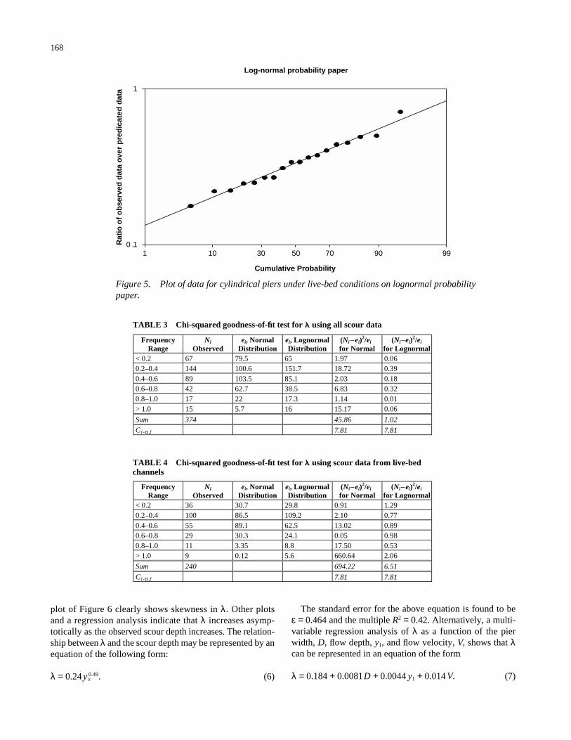
168

plot of Figure 6 clearly shows skewness in λ. Other plotsand a regression analysis indicate that λ increases asymp-totically as the observed scour depth increases. The relation-ship between λ and the scour depth may be represented by anequation of the following form:

λ = 0.24 ys0.49. (6)

The standard error for the above equation is found to be ε = 0.464 and the multiple R2 = 0.42. Alternatively, a multi-variable regression analysis of λ as a function of the pierwidth, D, flow depth, y1, and flow velocity, V, shows that λcan be represented in an equation of the form

λ = 0.184 + 0.0081D + 0.0044 y1 + 0.014 V. (7)

Log-normal probability paper

Cumulative Probability

1 10 30 50 70 90 99

Rat

io o

f o

bse

rved

dat

a o

ver

pre

dic

ated

dat

a

0 .1

1

Figure 5. Plot of data for cylindrical piers under live-bed conditions on lognormal probabilitypaper.

TABLE 3 Chi-squared goodness-of-fit test for using all scour data

Frequency Range

Ni

Observed ei, Normal

Distribution ei, Lognormal Distribution

(Ni –ei)2/ei

for Normal (Ni –ei)

2/ei for Lognormal

< 0.2 67 79.5 65 1.97 0.06 0.2–0.4 144 100.6 151.7 18.72 0.39 0.4–0.6 89 103.5 85.1 2.03 0.18 0.6–0.8 42 62.7 38.5 6.83 0.32 0.8–1.0 17 22 17.3 1.14 0.01 > 1.0 15 5.7 16 15.17 0.06

Sum 374 45.86 1.02

C1- α ,f 7.81 7.81

TABLE 4 Chi-squared goodness-of-fit test for using scour data from live-bedchannels

Frequency Range

Ni

Observed ei, Normal

Distribution ei, Lognormal Distribution

(Ni –ei)2/ei

for Normal(Ni –ei)

2/ei for Lognormal

< 0.2 36 30.7 29.8 0.91 1.29 0.2–0.4 100 86.5 109.2 2.10 0.77 0.4 –0.6 55 89.1 62.5 13.02 0.89 0.6–0.8 29 30.3 24.1 0.05 0.98 0.8–1.0 11 3.35 8.8 17.50 0.53 > 1.0 9 0.12 5.6 660.64 2.06

Sum 240 694.22 6.51

C1- α ,f 7.81 7.81

169

TABLE 6 Chi-squared goodness-of-fit test for using scour data of cylindricalpiers in live-bed channels

Frequency Range

Ni

Observed ei, Normal

Distribution ei, Lognormal Distribution

(Ni –ei)2/ei

for Normal (Ni –ei)

2/ei

for Lognormal < 0.2 1 2.15 1.31 0.62 0.07 0.2–0.3 6 3.93 5.52 1.09 0.04 0.3–0.4 5 5.31 5.66 0.02 0.08 0.4–0.5 4 4.16 3.22 0.01 0.19 0.5–0.6 1 1.88 1.41 0.41 0.12 0.6–0.7 0 0.49 0.55 0.49 0.55 > 0.7 1 0.08 0.33 10.54 1.36 Sum 18 13.18 2.42 C1– α ,f 9.49 9.49

TABLE 5 Chi-squared goodness-of-fit test for using scour data of roundedpiers in live-bed channels

Frequency Range

Ni

Observed ei, Normal

Distribution ei, Lognormal Distribution

(Ni –ei)2/ei

for Normal (Ni –ei)

2/ei for Lognormal

< 0.2 7 6.14 5.96 0.12 0.18 0.2–0.3 10 7.30 11.25 1.00 0.14 0.3–0.4 7 10.00 10.59 0.90 1.21 0.4–0.5 9 10.16 7.60 0.13 0.26 0.5–0.6 6 7.65 4.89 0.36 0.25 0.6–0.7 5 4.28 3.01 0.12 1.32 > 0.7 4 2.47 4.71 0.95 0.11 Sum 48 3.58 3.47 C1– α ,f 9.49 9.49

for 48 samples

ln(observed scour depth (ft))

-1 0 1 2 3

lam

da

0.0

0.1

0.2

0.3

0.4

0.5

0.6

0.7

0.8

Figure 6. Plot of modeling variable, λ, versus observed scour depth.

170

The above equation is executed for the 48 samples ofrounded piers in noncohesive soils under live-load conditions.In fact, using an analysis of variance, it was found that the effectof the pier shape on the average value of λ was not statisticallysignificant given the high observed standard deviations.

To account for the skewness in λ that is caused by the useof the HEC-18 equations, an alternative method of analysisis suggested as described in Section 3 of this appendix.

3. ALTERNATIVE RELIABILITY MODEL FORSCOUR

Appendix C of this report presented the results of a reliabil-ity analysis of bridge piers subjected to scour. The model usedin Appendix C was based on data that were previously avail-able in the literature and assumed that the modeling variable λis uniform for all cases. The existence of the extensive data-base published by Landers and Mueller (1996) provides aunique opportunity to come up with an alternative empiricalmodel for predicting scour depths based on a multivariableregression analysis. Several alternative regression models havebeen analyzed, including a regression effected on the wholedata set consisting of 374 samples, on the 48 samples for therounded piles in noncohesive soils, and on the combinationof rounded and cylindrical piers.

Based on the parameters tabulated by Landers and Mueller(1996) and after several trials to identify the parameters thatcontrol the scour depth, the regression equation for the total374 sample size was selected to be of the following form:

ln (scour) ∼ shape + bed-load transport + ln (pier width) + ln (flow depth) (8)+ ln (flow velocity)

where ln is the log function. The regression coefficientsobtained using the S+ computer package are tabulated as

shown in Table 7; the residual standard error was found to be0.56, and the term R2 = 0.53.

The regression analysis of the 48 samples of rounded piersin noncohesive soils was performed using a model of the fol-lowing form:

ln.(scour) ∼ ln (pier width) + ln (flow depth) + ln (flow velocity)

(9)

In this case, the regression coefficients are listed in Table 8.The residual standard error was found to be 0.41 on 44degrees of freedom and the term R2 is 0.83.

The analysis of the residuals for the 48 sample points asplotted in Figures 7 through 9 shows that the points areevenly spread around the value of 0.0 and that they can bereasonably well represented by a normal distribution.

The use of the regression results in the reliability analysismay be effected by replacing the failure function of Equa-tion 3 by the equation

Z = ydesign − yregression (10)

where for rounded piers in noncohesive soils yregression is cal-culated from

ln yregression = −2.08 + 0.63 ln D + 0.48 ln y1

+ 0.61 ln V + ε (11)

where

D = the pier diameter,y1 = the flow depth,V = the flow velocity, andε = the residual error.

TABLE 8 Coefficients of regression analysis for 48 samples of rounded pier data

Coefficients Value Standard Error t Value Pr ( > |t| )

(Intercept) –2.08 0.30 –6.98 0.0000 ln.width.b 0.63 0.14 4.62 0.0000 ln.flow.depth 0.48 0.13 4.10 0.0002 ln.flow.vel 0.61 0.13 4.78 0.0000

TABLE 7 Coefficients of regression analysis for all 374 samples of data

Coefficients Value Standard Error t Value Pr ( > |t| )

(Intercept) –0.60 0.10 –6.10 0.000 Shape 1 –0.19 0.11 –1.68 0.094 Shape 2 –0.10 0.04 –2.47 0.014 Shape 3 –0.02 0.03 –0.67 0.500 Shape 4 0.02 0.02 0.96 0.338 Bed.load 0.16 0.03 4.60 0.000 ln.width.b 0.66 0.07 9.58 0.000 ln.flow.depth 0.20 0.04 5.04 0.000 ln.flow.vel 0.12 0.05 2.15 0.032

171

As explained above, D is a deterministic variable since thepier diameter can be accurately known even before the actualconstruction of the pier; y1 and V are random variables thatdepend on Manning’s roughness coefficient and the 75-yearmaximum discharge rate, which are random variables havingthe properties listed in Table 8. Based on the analysis of theresiduals effected in this section of the report, ε may be con-sidered to follow a normal distribution with mean equal tozero and a standard deviation equal to 0.41.

Using Equation 10 in a Monte Carlo simulation as describedin Section 2 of Appendix C of this report for the Schohaire

River, data would lead to the results shown in Figure 10. Theplot shows that if the HEC-18 equation is used for designingthe bridge pier, then the critical design scour depth should bey = 17.3 ft. The reliability index obtained for such a design isβ = 0.47. The reliability index increases to β =2.71 when thescour depth is designed to be twice the value of HEC-18 (i.e.,yactual/yHEC-18 = 2.0 or yactual = 34.6 ft).

A slight difference in the results is observed when yregression

is calculated based on the regression equation obtained whenthe full set of 374 samples is used (i.e., from Equation 8).These results are also shown in Figure 10. In this case, the

Fitted : ln.width.b + ln.flow.depth + ln.flow.vel

Res

idua

ls

0.0 0.5 1.0 1.5 2.0 2.5

-0.5

0.0

0.5

33 3

7

Figure 7. Plot of residuals for 48 samples of rounded piers.

Fitted : ln.width.b + ln.flow.depth + ln.flow.vel

ln.s

cour

.obs

0.0 1.00.5 1.5 2.0 2.5

01

23

Figure 8. Comparison of regression results to observed scour depth.

172

reliability index of β = 0.58 is obtained when the foundationis designed for a critical depth of 17.32 ft as stipulated fromthe HEC-18 equations. The reliability index is 2.45 when thefoundation depth is set at 34.64 ft. The small differencesobserved between the results obtained from Equation 8 andEquation 9 are due to the larger standard regression errorobtained from Equation 8 that uses all 378 sample points.

The reliability analysis is subsequently performed for thefive different rivers that were analyzed in Appendix C: theSchohaire, Mohawk, Sandusky, Cuyahoga, and Rocky Rivers.These relatively small rivers are selected because they pro-

duce 100-year flood depths ranging from 8.5 ft to 21 ft, whichare appropriate for the bridge configuration under investiga-tion as described in Appendix C. As was done in Appendix C,two cases are considered: (1) the case in which the bents areformed by one column each and (2) the case in which the bentsare formed by two columns. The results of the reliability analy-sis for each case are presented in Figures 11 and 12.

Tables 9 and 10 also provide a summary of the resultsobtained using this alternative reliability model for the bridgewith the one-column bent and for the two-column bent. Theresults illustrate how the reliability index decreases for the

Quantiles of Standard Normal

Res

idua

ls

-2 -1 0 1 2

-0.5

0.00

0.5

33 3

7

Figure 9. Plot of residual versus standard normal quantiles.

Reliability index for scour depth exceedance (one column river Schohaire)

-4

-3

-2

-1

0

1

2

3

4

5

1.210.80.60.4 2.82.62.42.221.81.61.4 3.23 3.63.4

Ydepth / Ydesign scour depth(1.0 is the HEC-18 design scour depth =17.3 ft)

Bet

a

48 ln.scour.obs

374 ln.scour.obs

Figure 10. Plot of reliability index versus foundation depth.

173

rivers with higher discharge rates varying from β = 1.66 forthe Rocky River to β = 0.47 for the Schohaire River. Thelower beta for the rivers with higher discharge rates reflectsthe influence of a lower modeling variable, λ, for high valuesof scour depths. Such results indicate that the HEC-18 equa-tion becomes less conservative as the expected scour depthincreases. The average reliability index for the cases consid-

ered is on the order of 1.08. If one is to group the rivers intothree categories—high discharge rates (Schohaire), mediumdischarge rates (Mohawk and Sandusky), and small dis-charge rates (Cuyahoga and Rocky)—then the average betawould be close to β = 1.0. This value is clearly lower than theβ = 1.40 observed in Appendix C when the reliability modelemploying a uniform modeling variable is used.

Reliability index for scour depth exceedance (one column bent)

-4

-3

-2

-1

0

1

2

3

4

5

0.4 0 .9 1 .4 1 .9 2 .4 2 .9 3 .4 3 .9 4 .4

Ycr/Scour depth (1.0 is the scour depth of of Design)

Bet

a

Schohaire

Mohawk

Sadusky

Cuyahoga

Rocky

Figure 11. Plot of reliability index for one-column bent for five river discharges.

Reliability index for scour data depth exceedance (two column bent)

-4

-3

-2

-1

0

1

2

3

4

5

0.4 0 .9 1 .4 1 .9 2 .4 2 .9 3 .4 3 .9

Ycr/Scour depth(1.0 is the scour depth of design)

Bet

a

Schohaire

Mohawk

Sadusky

Cuyahoga

Rocky

Figure 12. Plot of reliability index for two-column bent for five river discharges.

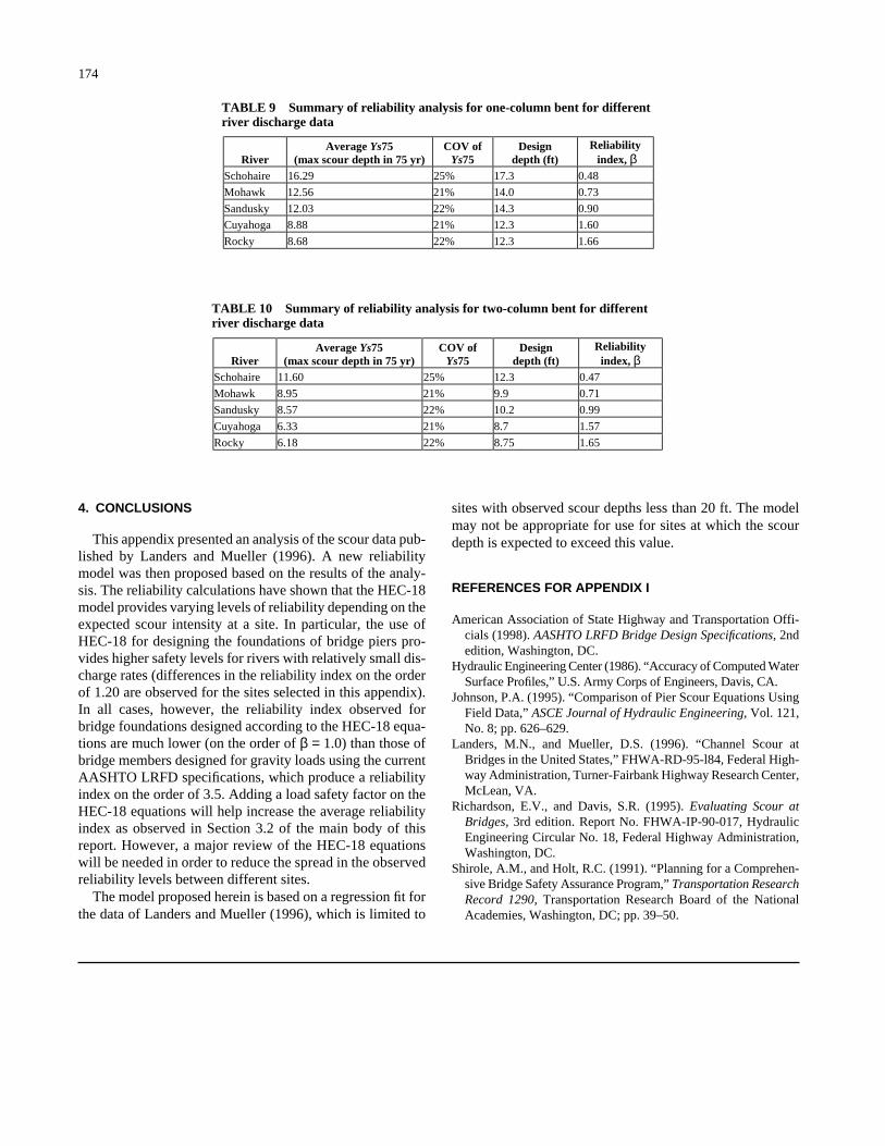
174

4. CONCLUSIONS

This appendix presented an analysis of the scour data pub-lished by Landers and Mueller (1996). A new reliabilitymodel was then proposed based on the results of the analy-sis. The reliability calculations have shown that the HEC-18model provides varying levels of reliability depending on theexpected scour intensity at a site. In particular, the use ofHEC-18 for designing the foundations of bridge piers pro-vides higher safety levels for rivers with relatively small dis-charge rates (differences in the reliability index on the orderof 1.20 are observed for the sites selected in this appendix).In all cases, however, the reliability index observed forbridge foundations designed according to the HEC-18 equa-tions are much lower (on the order of β = 1.0) than those ofbridge members designed for gravity loads using the currentAASHTO LRFD specifications, which produce a reliabilityindex on the order of 3.5. Adding a load safety factor on theHEC-18 equations will help increase the average reliabilityindex as observed in Section 3.2 of the main body of thisreport. However, a major review of the HEC-18 equationswill be needed in order to reduce the spread in the observedreliability levels between different sites.

The model proposed herein is based on a regression fit forthe data of Landers and Mueller (1996), which is limited to

sites with observed scour depths less than 20 ft. The modelmay not be appropriate for use for sites at which the scourdepth is expected to exceed this value.

REFERENCES FOR APPENDIX I

American Association of State Highway and Transportation Offi-cials (1998). AASHTO LRFD Bridge Design Specifications, 2ndedition, Washington, DC.

Hydraulic Engineering Center (1986). “Accuracy of Computed WaterSurface Profiles,” U.S. Army Corps of Engineers, Davis, CA.

Johnson, P.A. (1995). “Comparison of Pier Scour Equations UsingField Data,” ASCE Journal of Hydraulic Engineering, Vol. 121,No. 8; pp. 626–629.

Landers, M.N., and Mueller, D.S. (1996). “Channel Scour atBridges in the United States,” FHWA-RD-95-l84, Federal High-way Administration, Turner-Fairbank Highway Research Center,McLean, VA.

Richardson, E.V., and Davis, S.R. (1995). Evaluating Scour atBridges, 3rd edition. Report No. FHWA-IP-90-017, HydraulicEngineering Circular No. 18, Federal Highway Administration,Washington, DC.

Shirole, A.M., and Holt, R.C. (1991). “Planning for a Comprehen-sive Bridge Safety Assurance Program,” Transportation ResearchRecord 1290, Transportation Research Board of the NationalAcademies, Washington, DC; pp. 39–50.

TABLE 10 Summary of reliability analysis for two-column bent for differentriver discharge data

River Average Ys75

(max scour depth in 75 yr) COV of

Ys75 Design

depth (ft) Reliability

index, β Schohaire 11.60 25% 12.3 0.47

Mohawk 8.95 21% 9.9 0.71

Sandusky 8.57 22% 10.2 0.99

Cuyahoga 6.33 21% 8.7 1.57

Rocky 6.18 22% 8.75 1.65

TABLE 9 Summary of reliability analysis for one-column bent for differentriver discharge data

River Average Ys75

(max scour depth in 75 yr) COV of

Ys75 Design

depth (ft) Reliability index, β

Schohaire 16.29 25% 17.3 0.48

Mohawk 12.56 21% 14.0 0.73

Sandusky 12.03 22% 14.3 0.90

Cuyahoga 8.88 21% 12.3 1.60

Rocky 8.68 22% 12.3 1.66

Abbreviations used without definitions in TRB publications:

AASHO American Association of State Highway OfficialsAASHTO American Association of State Highway and Transportation OfficialsASCE American Society of Civil EngineersASME American Society of Mechanical EngineersASTM American Society for Testing and MaterialsFAA Federal Aviation AdministrationFHWA Federal Highway AdministrationFRA Federal Railroad AdministrationFTA Federal Transit AdministrationIEEE Institute of Electrical and Electronics EngineersITE Institute of Transportation EngineersNCHRP National Cooperative Highway Research ProgramNCTRP National Cooperative Transit Research and Development ProgramNHTSA National Highway Traffic Safety AdministrationSAE Society of Automotive EngineersTCRP Transit Cooperative Research ProgramTRB Transportation Research BoardU.S.DOT United States Department of Transportation