Embed Size (px)
Citation preview

Default Values for Highway Capacity and
Level of Service Analyses
NATIONALCOOPERATIVE HIGHWAYRESEARCH PROGRAMNCHRP
REPORT 599

TRANSPORTATION RESEARCH BOARD 2008 EXECUTIVE COMMITTEE*
OFFICERS
CHAIR: Debra L. Miller, Secretary, Kansas DOT, Topeka VICE CHAIR: Adib K. Kanafani, Cahill Professor of Civil Engineering, University of California, Berkeley EXECUTIVE DIRECTOR: Robert E. Skinner, Jr., Transportation Research Board
MEMBERS
J. Barry Barker, Executive Director, Transit Authority of River City, Louisville, KYAllen D. Biehler, Secretary, Pennsylvania DOT, HarrisburgJohn D. Bowe, President, Americas Region, APL Limited, Oakland, CALarry L. Brown, Sr., Executive Director, Mississippi DOT, JacksonDeborah H. Butler, Executive Vice President, Planning, and CIO, Norfolk Southern Corporation, Norfolk, VAWilliam A.V. Clark, Professor, Department of Geography, University of California, Los AngelesDavid S. Ekern, Commissioner, Virginia DOT, RichmondNicholas J. Garber, Henry L. Kinnier Professor, Department of Civil Engineering, University of Virginia, CharlottesvilleJeffrey W. Hamiel, Executive Director, Metropolitan Airports Commission, Minneapolis, MNEdward A. (Ned) Helme, President, Center for Clean Air Policy, Washington, DCWill Kempton, Director, California DOT, SacramentoSusan Martinovich, Director, Nevada DOT, Carson CityMichael D. Meyer, Professor, School of Civil and Environmental Engineering, Georgia Institute of Technology, AtlantaMichael R. Morris, Director of Transportation, North Central Texas Council of Governments, ArlingtonNeil J. Pedersen, Administrator, Maryland State Highway Administration, BaltimorePete K. Rahn, Director, Missouri DOT, Jefferson CitySandra Rosenbloom, Professor of Planning, University of Arizona, TucsonTracy L. Rosser, Vice President, Corporate Traffic, Wal-Mart Stores, Inc., Bentonville, ARRosa Clausell Rountree, Executive Director, Georgia State Road and Tollway Authority, AtlantaHenry G. (Gerry) Schwartz, Jr., Chairman (retired), Jacobs/Sverdrup Civil, Inc., St. Louis, MOC. Michael Walton, Ernest H. Cockrell Centennial Chair in Engineering, University of Texas, AustinLinda S. Watson, CEO, LYNX–Central Florida Regional Transportation Authority, OrlandoSteve Williams, Chairman and CEO, Maverick Transportation, Inc., Little Rock, AR
EX OFFICIO MEMBERS
Thad Allen (Adm., U.S. Coast Guard), Commandant, U.S. Coast Guard, Washington, DCJoseph H. Boardman, Federal Railroad Administrator, U.S.DOTRebecca M. Brewster, President and COO, American Transportation Research Institute, Smyrna, GAPaul R. Brubaker, Research and Innovative Technology Administrator, U.S.DOTGeorge Bugliarello, Chancellor, Polytechnic University of New York, Brooklyn, and Foreign Secretary, National Academy of Engineering,
Washington, DCJ. Richard Capka, Federal Highway Administrator, U.S.DOT Sean T. Connaughton, Maritime Administrator, U.S.DOTLeRoy Gishi, Chief, Division of Transportation, Bureau of Indian Affairs, U.S. Department of the Interior, Washington, DCEdward R. Hamberger, President and CEO, Association of American Railroads, Washington, DCJohn H. Hill, Federal Motor Carrier Safety Administrator, U.S.DOTJohn C. Horsley, Executive Director, American Association of State Highway and Transportation Officials, Washington, DCCarl T. Johnson, Pipeline and Hazardous Materials Safety Administrator, U.S.DOTJ. Edward Johnson, Director, Applied Science Directorate, National Aeronautics and Space Administration, John C. Stennis Space Center, MSWilliam W. Millar, President, American Public Transportation Association, Washington, DCNicole R. Nason, National Highway Traffic Safety Administrator, U.S.DOTJeffrey N. Shane, Under Secretary for Policy, U.S.DOTJames S. Simpson, Federal Transit Administrator, U.S.DOTRobert A. Sturgell, Acting Administrator, Federal Aviation Administration, U.S.DOTRobert L. Van Antwerp (Lt. Gen., U.S. Army), Chief of Engineers and Commanding General, U.S. Army Corps of Engineers, Washington, DC
*Membership as of January 2008.

TRANSPORTAT ION RESEARCH BOARDWASHINGTON, D.C.
2008www.TRB.org
N A T I O N A L C O O P E R A T I V E H I G H W A Y R E S E A R C H P R O G R A M
NCHRP REPORT 599
Subject Areas
Planning and Administration
Default Values for Highway Capacity and
Level of Service Analyses
John D. Zegeer
Mark Vandehey
Miranda Blogg
Khang Nguyen
Michael EretiKITTELSON & ASSOCIATES, INC.
Fort Lauderdale, FL
Research sponsored by the American Association of State Highway and Transportation Officials in cooperation with the Federal Highway Administration
NATIONAL COOPERATIVE HIGHWAYRESEARCH PROGRAM
Systematic, well-designed research provides the most effective
approach to the solution of many problems facing highway
administrators and engineers. Often, highway problems are of local
interest and can best be studied by highway departments individually
or in cooperation with their state universities and others. However, the
accelerating growth of highway transportation develops increasingly
complex problems of wide interest to highway authorities. These
problems are best studied through a coordinated program of
cooperative research.
In recognition of these needs, the highway administrators of the
American Association of State Highway and Transportation Officials
initiated in 1962 an objective national highway research program
employing modern scientific techniques. This program is supported on
a continuing basis by funds from participating member states of the
Association and it receives the full cooperation and support of the
Federal Highway Administration, United States Department of
Transportation.
The Transportation Research Board of the National Academies was
requested by the Association to administer the research program
because of the Board’s recognized objectivity and understanding of
modern research practices. The Board is uniquely suited for this
purpose as it maintains an extensive committee structure from which
authorities on any highway transportation subject may be drawn; it
possesses avenues of communications and cooperation with federal,
state and local governmental agencies, universities, and industry; its
relationship to the National Research Council is an insurance of
objectivity; it maintains a full-time research correlation staff of
specialists in highway transportation matters to bring the findings of
research directly to those who are in a position to use them.
The program is developed on the basis of research needs identified
by chief administrators of the highway and transportation departments
and by committees of AASHTO. Each year, specific areas of research
needs to be included in the program are proposed to the National
Research Council and the Board by the American Association of State
Highway and Transportation Officials. Research projects to fulfill these
needs are defined by the Board, and qualified research agencies are
selected from those that have submitted proposals. Administration and
surveillance of research contracts are the responsibilities of the National
Research Council and the Transportation Research Board.
The needs for highway research are many, and the National
Cooperative Highway Research Program can make significant
contributions to the solution of highway transportation problems of
mutual concern to many responsible groups. The program, however, is
intended to complement rather than to substitute for or duplicate other
highway research programs.
Published reports of the
NATIONAL COOPERATIVE HIGHWAY RESEARCH PROGRAM
are available from:
Transportation Research BoardBusiness Office500 Fifth Street, NWWashington, DC 20001
and can be ordered through the Internet at:
http://www.national-academies.org/trb/bookstore
Printed in the United States of America
NCHRP REPORT 599
Project 3-82ISSN 0077-5614ISBN: 978-0-309-09931-8Library of Congress Control Number 2008925081
© 2008 Transportation Research Board
COPYRIGHT PERMISSION
Authors herein are responsible for the authenticity of their materials and for obtainingwritten permissions from publishers or persons who own the copyright to any previouslypublished or copyrighted material used herein.
Cooperative Research Programs (CRP) grants permission to reproduce material in thispublication for classroom and not-for-profit purposes. Permission is given with theunderstanding that none of the material will be used to imply TRB, AASHTO, FAA, FHWA,FMCSA, FTA, or Transit Development Corporation endorsement of a particular product,method, or practice. It is expected that those reproducing the material in this document foreducational and not-for-profit uses will give appropriate acknowledgment of the source ofany reprinted or reproduced material. For other uses of the material, request permissionfrom CRP.
NOTICE
The project that is the subject of this report was a part of the National Cooperative HighwayResearch Program conducted by the Transportation Research Board with the approval ofthe Governing Board of the National Research Council. Such approval reflects theGoverning Board’s judgment that the program concerned is of national importance andappropriate with respect to both the purposes and resources of the National ResearchCouncil.
The members of the technical committee selected to monitor this project and to review thisreport were chosen for recognized scholarly competence and with due consideration for thebalance of disciplines appropriate to the project. The opinions and conclusions expressedor implied are those of the research agency that performed the research, and, while they havebeen accepted as appropriate by the technical committee, they are not necessarily those ofthe Transportation Research Board, the National Research Council, the AmericanAssociation of State Highway and Transportation Officials, or the Federal HighwayAdministration, U.S. Department of Transportation.
Each report is reviewed and accepted for publication by the technical committee accordingto procedures established and monitored by the Transportation Research Board ExecutiveCommittee and the Governing Board of the National Research Council.
The Transportation Research Board of the National Academies, the National ResearchCouncil, the Federal Highway Administration, the American Association of State Highwayand Transportation Officials, and the individual states participating in the NationalCooperative Highway Research Program do not endorse products or manufacturers. Tradeor manufacturers’ names appear herein solely because they are considered essential to theobject of this report.

CRP STAFF FOR NCHRP REPORT 599
Christopher W. Jenks, Director, Cooperative Research ProgramsCrawford F. Jencks, Deputy Director, Cooperative Research ProgramsB. Ray Derr, Senior Program OfficerEileen P. Delaney, Director of PublicationsKami Cabral, Editor
NCHRP PROJECT 3-82Field of Traffic—Area of Operations and Control
Robert W. Bryson, City of Milwaukee, Milwaukee, WI (Chair)Martin Guttenplan, Florida DOT, Tallahassee, FLMontasir M. Abbas, Virginia Polytechnic Institute and State University, Blacksburg, VAThomas W. “Bill” Brockenbrough, Jr., Delaware DOT, Dover, DEF. Thomas Creasey, American Consulting Engineers, PLC, Lexington, KYJeffery L. Memmott, Bureau of Transportation Statistics, Washington, DCNarasimha Murthy, Murthy Transportation Consultants, Inc., Fullerton, CADouglas Norval, Oregon DOT, Salem, ORRoger L. Russell, Charleston, WVZong Z. Tian, University of Nevada - Reno, Reno, NVJohn Halkias, FHWA LiaisonRichard A. Cunard, TRB Liaison
AUTHOR ACKNOWLEDGMENTS
The Highway Capacity Manual Default Value Guidebook was developed under NCHRP Project 3-82.The NCHRP Project 3-82 team consisted of Kittelson & Associates, Inc. (prime contractor), assisted byDr. James Bonneson (Texas Transportation Institute) and Dr. Fred Hall (McMaster University).
John D. Zegeer, P.E., PTOE, Senior Principal, Kittelson & Associates, Inc., was the principal investiga-tor. Additional Kittelson & Associates, Inc., staff who played key roles in the development of this Guide-book included Miranda Blogg, Khang Nguyen, Michael Ereti, and Mark Vandehey. Additional assistancein the data summary and analysis activities for various input parameters was provided by other Kittelsonstaff, including Cade Braud, Joey Bansen, Justin Bansen, Thuha Lyew, Gorken Mimioglu, Alek Pochowski,and Ning Zou. Terry Raddeman provided GIS graphical support and analysis of metropolitan area pop-ulations. Beverley King provided word processing and editorial assistance.
Finally, the project team would like to express its appreciation for the dedicated work of the NCHRPProject 3-82 panel. The majority of the panel members have been involved in the review of interim mate-rials and oversight of the findings throughout the project. The panel provided many thoughtful commentsthat have helped shape the current form of the Guidebook. The guidance provided by the NCHRP Pro-gram Officer, B. Ray Derr, is also greatly appreciated.
C O O P E R A T I V E R E S E A R C H P R O G R A M S

Based on the assembly of an extensive set of field data from across the United States, thisreport presents valuable information on the appropriate selection of default values whenanalyzing highway capacity and level of service. The report will be useful to planners, geo-metric designers, and traffic engineers who do not have ready access to field data for ananalysis. The report also describes how to prepare service volume tables, which can be a use-ful sketch planning technique.
The Year 2000 Highway Capacity Manual (HCM 2000) is the most extensively referenceddocument on highway capacity and quality-of-service computations in the United States.While the HCM 2000 focuses on providing state-of-the-art methodologies for operationalanalyses, it is also used in planning and preliminary engineering applications.
To assist engineers and planners in applying HCM methodologies, the HCM 2000includes default values for many of the more difficult-to-obtain input parameters and vari-ables. The HCM 2000 states: “A default value is a representative value that may be appro-priate in the absence of local data.” As a result of insufficient field data, the HCM 2000recommends only a single default value for many key data items, inadequately reflecting thevariety of traffic and facility conditions across the United States. Because of limitedresources or inexperience, analysts often use these default values inappropriately.
Under NCHRP Project 3-82, Kittelson & Associates, Inc., and their subcontractorsreviewed all of the input values in the HCM to determine how sensitive the analysis method-ologies are to them and the difficulty of obtaining non-default input values. They thenassembled field data from various sources on the critical values. A statistical analysis of thefield data was performed to develop guidance on the most appropriate default values to use.These recommended default values could be used in place of the default values provided inHCM 2000.
By B. Ray DerrStaff OfficerTransportation Research Board
F O R E W O R D

1 Summary1 Purpose of the Guidebook2 Findings3 Recommendations9 Use of Service Volume Tables
11 Chapter 1 Introduction
13 Chapter 2 Current Planning Practices13 History of HCM 200014 HCM 2000 Guidance on the Use of Default Values17 HCM Definitions18 Inventory of Default Values30 User Survey Results
31 Chapter 3 Recommended Default Values31 Defining Default Values by Category34 Data Sources and Calculation Methodology35 %HV for Uninterrupted Flow Facilities37 PHFs for Uninterrupted Flow Facilities43 %HV for Interrupted Flow Facilities47 PHFs for Interrupted Flow Facilities51 Base Saturation Flow Rates for Signalized Intersections53 Lane Utilization for Through Lanes at Signalized Intersections
55 Chapter 4 Guidance for Selecting Defaults55 Pedestrian Walking Speeds and Start-up Times at Signalized Intersections58 Interchange Ramp Terminals62 Driver Population Factors on Freeways65 Signal Density on Urban Streets66 Free-Flow Speed on Urban Streets73 Saturation Flow Rates and Lane Utilization Factors for Dual
and Triple Left-Turn Lanes
77 Chapter 5 Guidance for Preparing Service Volume Tables77 Sample Service Volume Tables79 Sensitivity Analysis
83 Appendix A Sensitivity Analysis
119 Appendix B Lane Utilization Adjustment Factors for Interchange Ramp Terminals
C O N T E N T S
The Highway Capacity Manual (HCM) is the authoritative source providing state-of-the-art methodologies for evaluating highway, transit, bicycle, and pedestrian facilities at both theoperational and planning levels. The methodologies that are provided in the HCM requireinput parameters that depend on, in many cases, detailed site-specific data.
An input parameter is a variable that is included in an equation because it has an influenceon the dependent variable and its value is likely to vary significantly over the range of possibleequation applications. Input parameters can be measured in the field or estimated usingapproximation techniques. Default values are sometimes used to represent input parametersbecause these input parameters tend to be difficult to measure (or estimate).
Default values may also be used for input parameters when those variables have minimalimpact on the outcome of the results. Thus, a default value is a representative value that maybe used in place of actual field data for estimating an input parameter. Default values aretypically used for planning applications. This occurs because many planning analyses are con-ducted for future conditions where the geometric and operational characteristics of the facil-ity are not known. Default values are also frequently used for operational analysis when fielddata have not been collected.
Purpose of the Guidebook
Many of the HCM default values are not always applicable to given local conditions. Thisis true because the default values are based on limited data collected over several years orthey are not provided. Prior to this project effort, no nationwide research effort had beenconducted to assemble field measurements to determine if the default values contained inthe HCM represent typical conditions.
This research effort was conducted to assemble field measurements for the relevant inputvariables. As a result of this effort, this Guidebook was prepared to assist users of the HCM inthe selection of default values for various HCM applications. First, appropriate default valuesthat should be used for inputs to HCM analyses were identified. Then, a guide to select defaultvalues for various applications was developed.
This Guidebook describes the use of the current default values contained in the HCM andtheir application in planning and operations analysis practices (Chapter 2). Changes to exist-ing default values in the HCM are recommended based on the analysis of an extensive set ofdata that was collected throughout the United States (Chapter 3). When field data were notavailable, guidance was developed (based on research results) to assist the analyst in estimat-ing appropriate default values (Chapter 4). Finally, guidance is provided on how to develop
1
S U M M A R Y
Default Values for Highway Capacityand Level of Service Analyses

service volume tables for freeways and urban streets using a range of default values (Chap-ter 5). In Appendix A, the sensitivity of the various default values on the analysis results isdescribed by showing the impact on the service measures for each HCM methodology wheredefault values are provided.
Findings
A detailed investigation of default values that are provided in HCM 2000 was con-ducted. The results of this investigation led to findings that are described in the followingthree categories:
• Existing HCM Guidance in the Use of Default Values• Inventory of Existing Default Values• Sensitivity of Default Values
Existing HCM Guidance in the Use of Default Values
Guidance on the use of default values is provided in Chapter 9, Analytical ProceduresOverview, of HCM 2000. A portion of that guidance is provided below.
“The analyst should observe the following suggestions when generating inputs to the analytical procedures.• If the input variable can be observed in the field, measure it in the field.• In performing a planning application for a facility not yet built, measure a similar facility in the area
that has conditions similar to those of the proposed facility.• If neither of the first two sources is available, rely on local policy or typical local/state values.• If none of the above sources is available, default values provided in Part II (Chapters 10 through 14)
of this manual may be used.”
Inventory of Existing Default Values
In Part II of HCM 2000, there are four chapters (Chapters 10 through 13) that contain atotal of 63 default values. These default values are used in eight methodologies. These method-ologies (and the number of default values that are provided for each of them) are providedbelow:
• Urban Streets (2)• Signalized Intersections (19)• Pedestrians (5)• Bicycles (3)• Multilane Highways (9)• Two-Lane Highways (11)• Basic Freeway Segments (8)• Ramps and Ramp Junctions (6)
In addition, there are default values provided for three general traffic characteristics inChapter 9 of HCM 2000. Table 3 in Chapter 2 of this Guidebook lists the default value for eachof these input parameters and identifies the original source that served as the basis for each ofthem.
Default values are not provided for the following methodologies:
• Two-way Stop-Controlled (TWSC) Intersections• All-way Stop-Controlled (AWSC) Intersections• Interchange Ramp Terminals
2 Default Values for Highway Capacity and Level of Service Analyses

• Freeway Facilities• Freeway Weaving• Transit (default values for this methodology are contained in the Transit Capacity and
Quality of Service Manual [TCQSM])
Sensitivity of Default Values
A sensitivity analysis was conducted for all 63 input parameters where HCM 2000 suggestsdefault values. The intent of this analysis was to determine which input parameters deservedfurther study based on the relative change in the relevant service measure due to the change inthe value of the input parameter. Those input parameters that had a high degree of impact onthe relevant service measures were recommended for further study. To facilitate the rankingof the input parameters, the following three thresholds were established.
• The input parameter has a low degree of sensitivity if varying the input parameter valuechanges the service measure by 0 to 10%.
• The input parameter has a moderate degree of sensitivity if varying the input parametervalue changes the service measure by 10 to 20%.
• The input parameter has a high degree of sensitivity if varying the input parameterchanges the service measure by more than 20%.
The following 19 input parameters had a high degree of sensitivity in influencing the ser-vice measure results:
• Urban Streets (1)—signal density• Signalized Intersections (7)—peak-hour factor (PHF), length of analysis period,
arrival type, adjusted saturation flow rate, lane width, percent heavy vehicle (%HV),lane utilization
• Pedestrians (4)—effective sidewalk width, street corner radius, pedestrian walking speed,pedestrian start-up time
• Bicycle paths (2)—PHF, bicycle speed• Multilane highways (2)—base free flow speed, PHF• Two-Lane Highways (0)—none• Basic Freeway Segments (3)—driver population factor (DPF), grade, PHF• Ramps and Ramp Junctions (0)—none
Recommendations
In general, input parameters that describe the facility type, area type, terrain type, and geo-metric configuration (such as lane width, segment length, and interchange spacing) are read-ily available to the analyst. Default values should not be used for these input parameters.Default values for the following input parameters should be developed based on existing HCMguidance:
• Signalized Intersections—length of analysis period, arrival type• Bicycle Paths—PHF, bicycle speed• Multilane Highways—basic free-flow speed (FFS)
The following input parameters should be measured in the field or on plan drawings:
• Signalized Intersections—lane width• Pedestrians—sidewalk width, street corner radius• Two-Lane Highways—length of passing lanes• Basic Freeway Segments—specific grade or general terrain
Default Values for Highway Capacity and Level of Service Analyses 3

The remaining input parameters that are highly sensitive can be broken into two categories.The first category is where data can be obtained and the default value may be confirmed,updated, or defined further. The second category is where data is not readily available; how-ever, guidance regarding the selection of an appropriate default value can be provided basedon research.
Recommended Default Values Based on Data
For the first category of input parameters, data was collected throughout the United States.The data were summarized by geographic region, metropolitan area size, hourly volume, timeof day, and other variables. These data were obtained from three sources: (1) NCHRP, FHWA,and state research projects, (2) governmental agencies (federal, state, county, and city files),and (3) “In-house” databases assembled from transportation projects.
Recommended default values based on the data collected for this project are summarizedin the following six subsections.
Heavy Vehicle Percentages for Uninterrupted Flow Facilities
1. Existing HCM Default ValuesFreeways and multilane highways—10% (rural) 5% (urban)Two-lane Highways—14% (rural) 2% (urban)
2. Variables ConsideredFreeway, multilane, and rural two-lane facilitiesTwo population categories for two-lane and multilane highways: 5,000 to 50,000 and lessthan 5,000Four population categories for freeways: less than 5,000; 5,000 to 50,000; 50,000 to 250,000;and greater than 250,000
3. Source of DataHighway Performance Monitoring System from FHWA
4. FindingsStatistical differences were identified among states within each region. Thus, a widevariation of %HV by state is evident.
5. Recommended Default ValueApply %HV that is specific to each state. See Chapter 3 of this Guidebook for those values.
PHFs for Uninterrupted Flow Facilities
1. Existing HCM Default Values0.88 (rural) and 0.92 (urban)
2. Variables ConsideredFreeway, multilane, and rural two-lane facilitiesThree time period categories (a.m., midday, and p.m.)Four geographic regionsFour city-size categories
3. Sources of DataCalifornia, Florida, Idaho, Ohio, Wisconsin
4. FindingsPHF did not vary by geographic region, time of day, or metro area size
5. Recommended Default ValueAlthough data were limited, the data generally support the continued use of the existingHCM Default Values. Caution should be used in low volume situations where lower PHFvalues are likely to occur.
4 Default Values for Highway Capacity and Level of Service Analyses
Heavy Vehicle Percentages for Interrupted Flow Facilities
1. Existing HCM Default Values2% (Signalized Intersections)
2. Variables ConsideredFour city-size categoriesFour geographic regionsThree time periods: (a.m., midday, and p.m.)Six volume categories
3. Sources of DataArizona, Idaho, California, Florida, Maryland, Oregon, Utah, Washington, Wisconsin
4. FindingsNo significant differences by region, city size, intersection type, or intersection control.Variation occurs in %HV by total entering volume and peak period.
5. Recommended Default ValueOverall, it appears that a %HV Default Value of 3% is appropriate. As volume decreases,the %HV tends to increase. The %HV increases with decreasing city size.
PHFs for Interrupted Flow Facilities
1. Existing HCM Default Values0.92 (Signalized Intersections)
2. Variables ConsideredSignalized Intersections and Unsignalized Intersections (TWSC and AWSC)Four city-size categoriesFive geographic regionsSix volume categoriesThree time period categories (a.m., midday, and p.m.)
3. Sources of DataArizona, Idaho, California, Florida, Maryland, Oregon, Utah, Washington, Delaware,Wisconsin
4. FindingsNo significant differences by region, city size, intersection type, or intersection control.Caution: PHF becomes lower than the HCM Default Value when total entering volume isless than 1,000 vehicles.
5. Recommended Default ValueThe current default value of 0.92 should be used when the total entering volume is greaterthan 1,000 vehicles. Consider using a PHF of 0.90 or less when the total entering volume isless than 1,000 vehicles. The major street PHF can be used directly as an estimate of the inter-section PHF, when the side street volumes are not readily available for planning applications.
Base Saturation Flow Rates for Signalized Intersections
1. Existing HCM Default Values1,900 passenger cars per lane per hour (pcplph)
2. Variables ConsideredFour city-size categoriesFour geographic regions
3. Sources of DataArizona, Florida, Maryland, Indiana, Oregon, Texas, Nevada
4. FindingsWhen the observed base saturation flow rate is weighted by the number of headway obser-vations that make up the mean at each site, the resulting mean is 1,894 pcplph (for largercities).
Default Values for Highway Capacity and Level of Service Analyses 5
5. Recommended Default ValuesThe HCM default value of 1,900 is reasonable for metropolitan areas of greater than250,000. A default value of 1,750 should be used for metropolitan areas of less than250,000.
Lane Utilization for Through Lanes at Signalized Intersections
1. Existing HCM Default Values0.952 (2 through lanes)0.908 (3 through lanes)
2. Variables ConsideredNumber of lanes in lane group
3. Sources of DataArizona, District of Columbia, Indiana, Oregon, Florida, Washington
4. FindingsFor through lane groups with 2 and 3 lanes in the group, the measured lane utilizationadjustment factors were very similar to the HCM Default Values. Caution: Lane utiliza-tion values can be significantly influenced by the presence of freeway ramps located down-stream of the intersection.
5. Recommended Default ValueAlthough data were limited, the data generally support the continued use of the existingHCM Default Values.
Guidance on Default Values Based on Research Studies
This chapter provides information for input parameters where field data were not avail-able. Default value guidance was developed based on a review of relevant research literaturefor six input parameters.
Pedestrian Walking Speeds and Start-up Times at Signalized Intersections
1. Existing HCM Default Values4 ft/s (walking speed) at a signalized crosswalk for 15 percentile population(HCM assumes 4 ft/s for 0–20% elderly pedestrians and 3.3 ft/s with greater than 20%elderly pedestrians)3.2 s (start-up time) at a signalized crosswalk for 15 percentile population
2. Sources of Dataa. Fitzpatrick/Brewer/Turner Research—3.77 and 3.03 ft/s walking speeds (younger and
older than 60 years, respectively). Recommends 3.5 ft/s for general population and3.0 ft/s for older population.
b. Gates/Noyce/Bill/Van Ee Research—range of 3.8 to 3.3 ft/s walking speeds dependingon age distribution
c. Knoblauch/Pietruchka/Nitzburg Research—3.97 and 3.08 ft/s walking speeds(younger and older than 65 years, respectively); 3.06 and 3.75 s start-up times
d. Public Right-of-Way Access Advisory Committee (2002 Guidelines)—3.0 ft/s for all ages3. Findings
In the next edition of the MUTCD, a walking speed of 3.5 ft/s will be assumed for a sig-nalized crosswalk when calculating the Flashing Don’t Walk (FDW) from the near sidecurb or shoulder to the far side of the traveled way or median of sufficient width forpedestrians to wait. The guidance will also include a separate calculation for the totalpedestrian time (Walk plus Flashing Don’t Walk) using a default walking speed of 3.0 ft/sfrom 6 ft behind the curb to the far side of the traveled way.
6 Default Values for Highway Capacity and Level of Service Analyses

4. Recommended Default ValueAt a signal, the total pedestrian crossing time and associated components should bedefined as follows:• Total Pedestrian Time (Walk + Flashing Don’t Walk) = 3.0 ft/s walking speed from
6 ft behind the curb to the far side of the traveled way or median of sufficient widthfor pedestrians to wait
• Pedestrian Clearance Time (Flashing Don’t Walk) = 3.5 ft/s from curb to curb• Walk interval = Total Pedestrian Time minus Pedestrian Clearance Time
Caution: Consider local traffic signal timing practices when determining pedestrian crossing times.
Interchange Ramp Terminals
1. Existing HCM Default ValuesNone
2. Default Values to Be Considereda. Lane utilization (external approaches only)b. Traffic pressure (a quantitative measure)c. Distance between intersections within an interchange
3. Sources of DataNew HCM Chapter 26. Chapter 26 covers diamond, partial cloverleaf (PARCLO), andsingle-point urban interchanges
4. Recommendations• The lane utilization adjustment factor (fLU) is an adjustment for base saturation flow
rate. fLU tables are provided in this Guidebook for seven interchange types.• Traffic pressure adjustment factor reflects aggressive driving behavior when shorter head-
ways are accepted during queue discharge. Adjustment factors are provided in this Guide-book for various cycle lengths and flow rates.
• Typical ranges of intersection separation distances (by interchange type) are provided in this Guidebook. Distances should be measured or taken from scaleddrawings.
Driver Population Factors on Freeways
1. Existing HCM Default Value1.00
2. Sources of DataUniversity of South Florida research report—Paper by Lu, Mierzejewski, Huang, andCleland (1997); Literature summary by and data from Al-Kaisy and Hall (2001)
3. FindingsDriver population factors were developed in this prior research on the basis of speed-flowdata.
4. Recommendationsa. A procedure is recommended in this Guidebook for estimating a driver population fac-
tor based on a comparison of (1) observed capacity when regular commuters are usingthe freeway and (2) observed capacity when a different driver population is using thefreeway. Caution: Local knowledge of the freeway system is required to determine when dif-ferent driver populations are likely to use the freeway system.
b. An example that illustrates the recommended methodology is provided.c. In general, HCM analyses should assume a driver population factor of 1.00. A lower
value should be used only when there are special circumstances, such as sporting eventsor tourist routes, and when it is possible to estimate the driver population factor usingthis methodology.
Default Values for Highway Capacity and Level of Service Analyses 7
Signal Density on Urban Streets
1. Existing HCM Default ValuesSignal Density (sig/mi)—0.8, 3, 6, 10 (Urban Street Classes I–IV)
2. RecommendationFor signal density, it is recommended that no default value be provided in the HCM. Ifthe number of signals per mile is not known, the analyst should conduct an assessmentto determine which intersections are likely to warrant signals.
Free-Flow Speed on Urban Streets
1. Existing HCM Default ValuesFree-flow speed (mph)—50, 40, 35, 30 (Urban Street Classes I–IV)
2. Existing HCM ProceduresFree-flow speed is defined as the speed that a through vehicle travels under low-volumeconditions (200 veh/hr/ln or less) when all signals are green for the entire trip. The cur-rent HCM procedure adjusts free-flow speed based on lane width, lateral clearance,median treatment, and access points.
3. Summary of Relevant ResearchThe relationship between free-flow speed and speed limit and the relationship betweenfree-flow speed and segment length are described in Chapter 4 of this report.
4. FindingsA procedure for estimating the base free-flow speed for an urban street is presented inChapter 4. The base free-flow speed is defined to be the free-flow speed on long street seg-ments such that the potential need to stop at the next signal does not have to be factoredinto the drivers’ speed choice.
5. RecommendationApply the equation provided in Chapter 4 of this Guidebook to determine the base freeflow speed. This procedure considers the posted speed limit, median type, and the pres-ence of curb and gutter.
Saturation Flow Rates and Lane Utilization Factors for Dual and Triple Left Turn Lanes
1. Existing HCM Default ValuesDual left turn lane utilization—0.971Triple left turn lane utilization—none providedDual and triple left turn saturation flow rate—none provided
2. Sources of Dataa. Spring, G. S., and Thomas, A. Double Left-Turn Lanes in Medium-Size Cities. Jour-
nal of Transportation Engineering, Vol. 125, March/April 1999: 138–143.b. Zegeer, J. D. Field Validation of Intersection Capacity Factors. Transportation
Research Record No. 1091 (1986): 67–77.c. Kagolanu, K., and Szplett, D. Saturation Flow Rates of Dual Left-Turn Lanes. Proceed-
ings of the Second International Symposium on Highway Capacity, 1994, Akcelik, R. (ed.),Volume 1, pp. 325–344.
d. Stokes, R. W., Messer, C. J., and Stover, V. G. Saturation Flows of Exclusive Double Left-Turn Lanes. Transportation Research Record No. 1091 (1986): 86–95.
e. Leonard II, J. D. Operational Characteristics of Triple Left Turns. TransportationResearch Record No. 1457 (1994): 104–110.
f. Sando, T., and Mussa, R. N. Site Characteristics Affecting Operation of Triple Left-TurnLanes. Transportation Research Record No. 1457 (1994): 104–110.
3. Recommendationsa. Left-Turn Lane Saturation Flow Adjustment Factor (Dual Left-Turn Lanes)—Set the
Default Value to 0.97.
8 Default Values for Highway Capacity and Level of Service Analyses
b. Left-Turn Lane Utilization Factor (Dual Left-Turn Lanes)—Maintain the currentDefault Value of 0.971 as suggested by the HCM.
c. Left-Turn Lane Saturation Flow Adjustment Factor (Triple Left-Turn Lanes)—Set theDefault Value to 0.97 until research can be completed.
d. Left-Turn Lane Utilization Factor (Triple Left-Turn Lanes)—Set the Default Value to0.971 as suggested by the HCM until further research is available.
Caution: Lane utilization values can be significantly influenced by the presence of freeway rampslocated downstream of the intersection.
Use of Service Volume Tables
A service volume table can provide an analyst with an estimate of the maximum number ofvehicles a facility can carry at a given level of service (LOS). The use of a service volume tableis most appropriate in certain planning applications where it is not feasible to evaluate everysegment or node within a study area. Examples of this would be city, county, or statewide plan-ning studies where the size of the study area makes it infeasible to conduct a capacity or levelof service analysis for every roadway segment. For these types of planning applications, thefocus of the effort is to simply highlight “potential” problem areas (for example locationswhere demand may exceed capacity or where a desired level of service threshold may beexceeded). For such applications, developing a service volume table can be a useful sketch plan-ning tool, provided the analyst understands the limitations of this method.
For the purposes of this Guidebook, an example of how to construct a service volume tablewas prepared for a basic freeway segment and for an urban street facility. These two facilitytypes were selected since they would likely be common applications of service volume tableswithin an urban area.
For the basic freeway segment example, the percent grade, PHF, and interchange densitywere varied over a range of values. The change in the maximum service volume at level of ser-vice “D” was evaluated. Varying the percent grade and PHF had a significant impact on theservice volume thresholds. Varying the interchange density had a moderate impact on the ser-vice volume thresholds.
For the urban street facility example, the effective green ratio, signal density, and PHF werevaried over a range of values. The change in the maximum service volume at level of service“D” was evaluated. Varying each of these three input parameters had a significant impact onthe service volume thresholds.
This chapter illustrated two points: (1) the importance of selecting appropriate default val-ues when constructing service volume tables (or conducting any planning or operationalanalysis that relies upon default values) and (2) some facilities are much more sensitive todefault values than others.
Default Values for Highway Capacity and Level of Service Analyses 9
For over fifty years, the Highway Capacity Manual (HCM) has been viewed as the authoritativereference document for use in conducting engineering analyses aimed at determining the opera-tional adequacy of a transportation facility. The fourth edition of the Highway Capacity Manual(HCM 2000) contains state-of-the-art methodologies for evaluating highway, transit, bicycle, andpedestrian facilities at both the operational and planning levels. The methodologies used to solvethese problems require input parameters that depend on, in many cases, detailed site-specific data.While site-specific data may be available for the short-term focus of operational analysis, such dataare often not available at the planning level. (This occurs because many planning analyses are con-ducted for future conditions where the geometric and operational characteristics of the facility arenot known.) In addition, field measurements are often not made when conducting operationalanalyses. For the purpose of determining and comparing intermediate to long-term systemimprovements with HCM methodologies, default values for these input parameters can be used.
A default value is defined as a representative value that may be appropriate for estimating aninput parameter in the absence of local data. Generic default values may be used for specific facil-ity analyses, but will produce less accurate results than locally developed default values. Where localsources are unavailable, the HCM default values provided in Part II (Chapters 7 through 14) areprovided.
Many of the HCM default values are not always applicable to given local conditions. This is truebecause the default values are based on limited data collected over several years or they are notprovided. Prior to this project effort, no nationwide research effort had been conducted to assem-ble field measurements to determine if the default values contained in the HCM represent typi-cal conditions.
The purpose of this Guidebook is to assist users of the HCM in the selection of default valuesfor various HCM applications. This Guidebook describes the use of the current default values con-tained in the HCM and their application in planning practices. The sensitivity of the variousdefault values on the analysis results is described. Changes to existing default values are recom-mended based on the analysis of an extensive set of data that was collected throughout the UnitedStates. When default values are not available, guidance is provided to help the analyst estimateappropriate values.
11
C H A P T E R 1
Introduction
The purpose of this chapter is to describe the development of the current HCM default valuesand the HCM recommended application of them. This chapter is divided into the following fivesections:
• History of HCM 2000• HCM 2000 guidance on the use of default values• HCM Definitions• Inventory of default values• User survey results
History of HCM 2000
The origins of the current procedures of HCM 2000 are based on a series of research effortswhich began in the late 1970s. A primary objective of these research efforts was to develop capac-ity and level of service procedures which were based on empirical data representing current traf-fic volume, traffic signal, and roadway characteristics. A number of these research efforts (NCHRPProject 2-28 series) culminated in the development of new procedures which were published inthe 1985 HCM. In the 1994 HCM update, the procedures contained in six of the twelve chapterswere the direct result of the research which focused on collection of large quantities of field data.Despite this effort, there were many specific areas of the 1994 HCM update that were primarilybased on theoretical models, sometimes “calibrated” with a small amount of data.
The 1997 HCM update revised the procedure for determining capacity and density of basicfreeway segments, based on the findings of NCHRP Project 3-45. The signalized intersectionchapter was updated based on findings from research on actuated traffic signals (NCHRP Project3-48). The delay equation was modified to account for signal coordination, oversaturation, vari-able length analysis periods, and the presence of initial queues at the beginning of the analysisperiod. Probably the biggest change in the 1997 HCM update was that control delay replacedstopped delay as the service measure. The chapter on unsignalized intersections was completelyrevised to incorporate the results of a nationwide research project that examined traffic opera-tions at two-way and four-way stop-controlled intersections (NCHRP Project 3-46). The arterialstreets chapter in the 1997 HCM incorporated the relevant changes from the signalized inter-section chapter as well. It also established a new arterial classification for high-speed facilities.In addition, the delay equation was modified to account for the effect of platoons fromupstream signalized intersections.
HCM 2000 was published in two versions: metric units and U.S. customary units. An accom-panying multimedia CD-ROM included interactive tutorials, example problems, and hyper-text. The number of chapters increased from 14 in the 1997 HCM to 31 in HCM 2000. HCM
13
C H A P T E R 2
Current Planning Practices

2000 was produced mainly from the NCHRP Project 3-55 series of research efforts that beganin 1995. Table 1 summarizes research efforts that have significantly contributed to the contentsof HCM 2000.
HCM 2000 Guidance on the Use of Default Values
HCM 2000 defines a default value as a representative value that may be appropriate for esti-mating an input parameter in the absence of local data. It further says that default values are tobe used for planning applications to estimate the level of service, the volume that can be accom-modated, or the number of lanes required. Chapter 9, Analytical Procedures Overview, describesguidance on the use of default values. This guideline states that
“Planning applications of the computation methods are described in Part III. Guidance for estimat-ing input values and selecting default values for planning applications is given in Part II (Chapters 10through 14). The analyst should observe the following suggestions when generating inputs to the ana-lytical procedures.
• If the input variable can be observed in the field, measure it in the field.• In performing a planning application for a facility not yet built, measure a similar facility in the area
that has conditions similar to those of the proposed facility.• If neither of the first two sources is available, rely on local policy or typical local/state values.• If none of the above sources is available, default values provided in Part II (Chapters 10 through 14)
of this manual may be used.”
14 Default Values for Highway Capacity and Level of Service Analyses
Table 1. List of research efforts with significant contribution to HCM 2000.
Research Project
Research Title Research Objective
NCHRP 3-55 Highway Capacity Manual for the Year 2000
Recommend user-preferred format and delivery system for HCM 2000
NCHRP 3-55(2) Techniques to Estimate Speeds and Service Volumes for Planning Applications
Develop extended planning techniques for estimating measures of effectiveness (MOEs)
NCHRP 3-55(2)A Planning Applications for the Year 2000 Highway Capacity Manual
Develop draft chapters related to planning for HCM 2000
NCHRP 3-55(3) Capacity and Quality of Service for Two- Lane Highways
Improve methods to determine capacity and quality of service of two-lane highways
NCHRP 3-55(4) Performance Measures and Levels of Service in the Year 2000 Highway Capacity Manual
Recommend MOEs and additional performance measures
NCHRP 3-55(5) Capacity and Quality of Service of Weaving Areas
Improve methods for capacity and qualityof service analyses of weaving areas
NCHRP 3-55(6) Production of the Year 2000 Highway Capacity Manual
Complete HCM 2000 document
TCRP A-07 Operational Analysis of Bus Lanes on Arterials
Develop procedures to determine capacity and level of service of bus flow on arterials
TCRP A-07A Operational Analysis of Bus Lanes on Arterials: Extended Field Investigations
Expand field testing and validation of procedures developed in TCRP Project A-07
TCRP A-15 Development of Transit Capacity and Quality of Service Principles, Practices, and Procedures
Provide transit input to HCM 2000
FHWA Capacity Analysis of Pedestrian and Bicycle Facilities Project (DTFH61-92-R- 00138)
Update method for analyzing effects of pedestrians and bicycles at signalized intersections; recommend improvements
FHWA Capacity and Level of Service Analysis for Freeway Systems Project (DTFH61- 95-Y-00086)
Develop procedure to determine capacity and level of service of a freeway facility
Source: HCM 2000, Exhibit 1-3.
NCHRP: National Cooperative Highway Research Program
TCRP: Transit Cooperative Research Program
FHWA: Federal Highway Administration
This guidance was formulated by the NCHRP Project 3-55(6) panel to suggest a clear directionon the use of HCM default values. The NCHRP Project 3-55(6) panel also believed that it wasimportant to add the following disclaimer when presenting example service volume tables in theHCM 2000.
“This table contains approximate values and is for illustrative purposes only. The values are highlydependent on the assumptions used. It should not be used for operational analyses or final design. Thistable was derived using the assumed values listed in the footnotes.”
The above disclaimer is intended to alert the user that the example service volume thresholdscould vary substantially based on selected default values and assumptions. The analyst should notuse service volume tables blindly as a decision making tool. It further states that default valuesused to generate example service volume tables should not be used as input variables for planningapplications.
To assist the user in obtaining input parameters from similar facilities, Chapter 8, Traffic Char-acteristics, presents several observed input and output parameters—primarily documented in theearly 1990s prior to the release of the 1994 HCM update. Most of the data were obtained from theFlorida Department of Transportation (FDOT) and the Minnesota Department of Transportation.Even though this information is outdated, it can provide HCM users with typical ranges of inputparameters for planning applications.
Appendix A of Chapter 9 in HCM 2000 contains guidelines on how to develop local default val-ues. These guidelines were developed as part of the NCHRP Project 3-55(2)A research effort. Someof the suggestions include
• The best method for determining local default values for traffic parameters is to measure a sam-ple of facilities in the field. If measuring local data is not feasible, an informal survey of localhighway operating agencies can be conducted to determine standard design practices for newfacilities and the condition of the facilities currently in place.
• Facilities can be stratified by area type and facility type to ensure reliable default values. Thechoice of categories is a local decision. Example sample stratification schemes may include cen-tral business district (CBD), suburban, and rural.
• It is suggested that the default value for each category be the arithmetic mean of the observa-tions. In addition, the variation in the observed value for each category should be compared withthe difference in the means for each category. Analysis of variance techniques may be used todetermine whether categories should be consolidated.
• The sample size required for each category can be determined by the desired accuracy in the resulting input estimate and the variation in the observed values. The following equa-tions are provided to determine the minimum sample size that will allow the analyst to com-pute the mean and estimate the margin of error in the estimated mean with 90% or betterconfidence.
Where
n = minimum number of observations to meet accuracy goal for mean;ξ = maximum desirable error in the estimate of the mean (at the desired confidence level);
ands = estimated standard deviation for the sample, computed using the following equation.
ns≥
( )4 2
2ξ
Current Planning Practices 15

Where
xi = ith observation of the value,x– = mean value of the observations, andn = number of observations.
The standard deviation is the most common measure of statistical dispersion, measuringhow widely spread the values in a data set are. If the data points are close to the mean, then thestandard deviation is small. If many data points are far from the mean, then the standard devi-ation is large.
Two observations can be made with regard to default values. One observation is that default val-ues are typically defined by transportation agencies responsible for the planning (or preliminaryengineering) of streets or highways. These default values are tailored to be representative of condi-tions in the agency’s jurisdiction. To ensure the accuracy and consistency of any evaluation,engineers within the agency draw on their familiarity with their transportation system to iden-tify appropriate default values. In some instances, several default values are identified for a givenvariable or factor, with the appropriate value being dependent on area type (i.e., urban, rural), areapopulation, or facility functional class.
A second observation is that default values for input variables are rarely a product ofresearch. Research is typically used to develop new models or evaluate existing models. Thedata collected for these purposes tend to support a new model’s framework or provide insightinto existing model accuracy. However, a database assembled for this type of research does notoften have the depth and breadth (from the standpoint of geography, area type, populationand functional class) to yield default values that are representative of every situation in whichthe model may be used.
In recognition of the aforementioned observations, researchers developing new models ofteninclude input variables and calibration factors in their models for which practitioners are expectedto provide the appropriate values. These values ensure the desired accuracy of the evaluation byadapting the equation to the unique features of the facility and the behavior of drivers in theirjurisdiction. Through experience, the practitioner determines which variables and factors requiremeasurement prior to each analysis and which can be defaulted.
Research publications rarely contain recommendations for default values for input vari-ables or calibration factors that have a significant influence on model accuracy. However,researchers do sometimes recommend default values for calibration factors that have amedium-to-small level of influence, and that are believed to be relatively stable (or invariant)among geographic regions, area types, population sizes, and functional classifications. Also,researchers explore correlations between various input variables and calibration factors forthe purpose of developing predictive equations. Such equations are used to estimate a factoras a function of one or more other, more readily available variables or factors. In this man-ner, the need to measure a specific factor for an evaluation is eliminated. As an example,research has shown start-up lost time is a function of saturation flow rate. This relationshipcan be used by practitioners to estimate start-up lost time without having to measure it in thefield or estimate it using a global constant. Similar relationships have been developed for esti-mating phase end lost time (as a function of approach speed) and free-flow speed (as a func-tion of speed limit).
sx x
n
i
2
2
1=
−⎛⎝⎜
⎞⎠⎟
−
∑ _
16 Default Values for Highway Capacity and Level of Service Analyses

HCM Definitions
This section defines several terms related to default values used in the analysis of interruptedand uninterrupted flow facilities and points.
Input Parameter is a variable that is included in an equation because it has an influence onthe dependent variable and its value is likely to vary significantly over the range of possibleequation applications. Hence, a value should be provided for each input parameter by analystseach time they use the equation to ensure an accurate estimate of the dependent variable. Inputparameters can be measured in the field or estimated using approximation techniques. Defaultvalues are sometimes used for input parameters that tend to be difficult to measure (or esti-mate) or those variables that have minimal impact on equation accuracy. Example inputparameters include turn movement volume, number of lanes, signal phase sequence, and sig-nal phase duration.
Calibration Factor is a variable that is included in an equation because it has an influenceon the dependent variable. It is assigned a constant value for most applications. It is used toadjust the equation’s predicted value such that this value reflects local conditions withoutbias. If the factor has a theoretic basis or is recognized as a universal constant, then the fac-tor is often referred to as an input parameter. Calibration factors can be measured using fielddata or estimated using regression analysis. Default values are sometimes used for those cal-ibration factors that tend to be difficult to measure (or estimate) or those factors that haveminimal impact on equation accuracy. Example calibration factors include base saturationflow rate, left-turn sneakers per cycle, start-up lost time, and passenger-car equivalent (PCE)for heavy vehicles.
Default Value is a constant to be used in an equation as a substitute for a field measured (or esti-mated) value. Default values can be used for input variables or calibration factors. The valueselected should represent a typical value for the conditions being analyzed. Default values are gen-erally used for planning, preliminary engineering, or other applications of the HCM that do notrequire the accuracy provided by a detailed operational evaluation.
Area Type is a characterization of the population in the vicinity of the subject facility. Four areatypes are typically used by planning agencies: urbanized, transitioning, urban, and rural. Anurbanized area is defined as an area having a population of 50,000 or more within a contiguousarea. A transitioning area is an area adjacent to an urbanized area and expected to become part ofthat area in the next 20 years. An urban area is an area with a population over 5,000 that is notconsidered to be urbanized or transitioning. A rural area is any area that is not urbanized, transi-tioning, or urban.
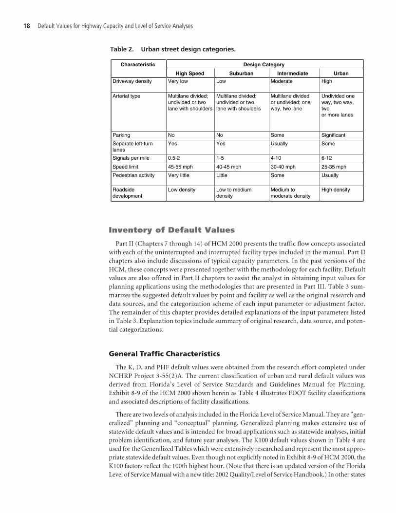
Design Category is a characterization of the geometric features of a street and its roadside envi-ronment. Four design categories are defined for urban streets in Chapter 10 of the HCM. Theyare listed in Table 2. The High Speed category describes streets with long distances between sig-nals, no adjacent parking, few driveways, and little roadside development. At the other end ofthe spectrum is the Urban category that describes streets with a short length, adjacent parking,many driveways, and considerable roadside development. Streets that fit the Urban category areoften found in downtown areas and CBDs.
Through Lanes are the total number of lanes in the roadway cross-section that extend for thefull length of the street segment (as measured between signalized intersections). A lane added anddropped at a signalized intersection may be included in the count of through lanes if the com-bined length of the add/drop lane allows the lane to operate at the intersection with an efficiencythat is near to (or exceeds) that of a through lane.
Current Planning Practices 17
Inventory of Default Values
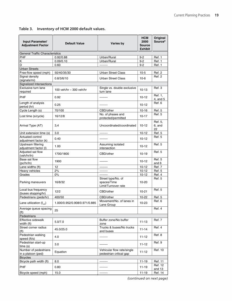
Part II (Chapters 7 through 14) of HCM 2000 presents the traffic flow concepts associatedwith each of the uninterrupted and interrupted facility types included in the manual. Part IIchapters also include discussions of typical capacity parameters. In the past versions of theHCM, these concepts were presented together with the methodology for each facility. Defaultvalues are also offered in Part II chapters to assist the analyst in obtaining input values forplanning applications using the methodologies that are presented in Part III. Table 3 sum-marizes the suggested default values by point and facility as well as the original research anddata sources, and the categorization scheme of each input parameter or adjustment factor.The remainder of this chapter provides detailed explanations of the input parameters listedin Table 3. Explanation topics include summary of original research, data source, and poten-tial categorizations.
General Traffic Characteristics
The K, D, and PHF default values were obtained from the research effort completed underNCHRP Project 3-55(2)A. The current classification of urban and rural default values wasderived from Florida’s Level of Service Standards and Guidelines Manual for Planning.Exhibit 8-9 of the HCM 2000 shown herein as Table 4 illustrates FDOT facility classificationsand associated descriptions of facility classifications.
There are two levels of analysis included in the Florida Level of Service Manual. They are “gen-eralized” planning and “conceptual” planning. Generalized planning makes extensive use ofstatewide default values and is intended for broad applications such as statewide analyses, initialproblem identification, and future year analyses. The K100 default values shown in Table 4 areused for the Generalized Tables which were extensively researched and represent the most appro-priate statewide default values. Even though not explicitly noted in Exhibit 8-9 of HCM 2000, theK100 factors reflect the 100th highest hour. (Note that there is an updated version of the FloridaLevel of Service Manual with a new title: 2002 Quality/Level of Service Handbook.) In other states
18 Default Values for Highway Capacity and Level of Service Analyses
Table 2. Urban street design categories.
Design Category Characteristic
High Speed Suburban Intermediate UrbanDriveway density Very low Low Moderate High
Arterial type Multilane divided; undivided or twolane with shoulders
Multilane divided; undivided or two lane with shoulders
Multilane divided or undivided; one way, two lane
Undivided one way, two way, twoor more lanes
Parking No No Some Significant
Separate left-turn lanes
Yes Yes Usually Some
Signals per mile 0.5-2 1-5 4-10 6-12
Speed limit 45-55 mph 40-45 mph 30-40 mph 25-35 mph
Pedestrian activity Very little Little Some Usually
Roadsidedevelopment
Low density Low to medium density
Medium tomoderate density
High density
Current Planning Practices 19
Table 3. Inventory of HCM 2000 default values.
Input Parameter/Adjustment Factor
Default Value Varies by
HCM2000
SourceExhibit
OriginalSourcea
General Traffic Characteristics PHF 0.92/0.88 Urban/Rural 9-2 Ref. 1 K 0.09/0.10 Urban/Rural 9-2 Ref. 1 D 0.60 -------- 9-2 Ref. 1 Urban Streets Free-flow speed (mph) 50/40/35/30 Urban Street Class 10-5 Ref. 2 Signal density (signals/mi)
0.8/3/6/10 Urban Street Class 10-6 Ref. 2
Signalized IntersectionsExclusive turn lanerequired
100 veh/hr – 300 veh/hr Single vs. double exclusiveturn lane
10-13Ref. 3
PHF 0.92 -------- 10-12 Ref. 1,4, and 5
Length of analysis period (hr)
0.25 -------- 10-12 Ref. 6
Cycle Length (s) 70/100 CBD/other 10-16 Ref. 5
Lost time (s/cycle) 16/12/8 No. of phases and protected/permitted
10-17Ref. 5
Arrival Type (AT) 3,4 Uncoordinated/coordinated 10-12 Ref. 5,6, and 22
Unit extension time (s) 3.0 -------- 10-12 Ref. 5 Actuated controladjustment factor (k)
0.40 -------- 10-12 Ref. 5
Upstream filteringadjustment factor (l)
1.00Assuming isolated intersection
10-12Ref. 5
Adjusted sat flow (veh/hr/ln)
1700/1800 CBD/other 10-19 Ref. 5
Base sat flow (pc/hr/ln)
1900 -------- 10-12 Ref. 5 and 6
Lane widths (ft) 12 -------- 10-12 Ref. 7 Heavy vehicles 2% -------- 10-12 Ref. 5 Grades 0% -------- 10-12 Ref. 4
Parking maneuvers 16/8/32 Street type/No. of spaces/TimeLimit/Turnover rate
10-20Ref. 5
Local bus frequency (buses stopping/hr)
12/2 CBD/other 10-21 Ref. 5
Pedestrians (peds/hr) 400/50 CBD/other 10-22 Ref. 5
Lane utilization (fLU) 1.000/0.952/0.908/0.971/0.885 Movement/No. of lanes inLane Group
10-23Ref. 6
Average queue spacing (ft)
25 Ref. 4
PedestriansEffective sidewalk width (ft)
5.0/7.0Buffer zone/No buffer zone
11-13Ref. 7
Street corner radius (ft)
45.0/25.0Trucks & buses/No trucks and buses
11-14Ref. 4
Pedestrian walking speed (ft/s)
4.0 -------- 11-12 Ref. 8
Pedestrian start-up time (s)
3.0 -------- 11-12 Ref. 9
Number of pedestriansin a platoon (ped)
EquationVehicular flow rate/single pedestrian critical gap
11-12Ref. 10
BicyclesBicycle path width (ft) 8.0 -------- 11-19 Ref. 11
PHF 0.80 -------- 11-19 Ref. 12 and 13
Bicycle speed (mph) 15.0 -------- 11-19 Ref. 14
(continued on next page)
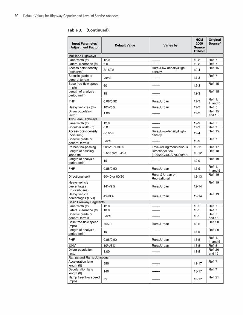
20 Default Values for Highway Capacity and Level of Service Analyses
Table 3. (Continued).
Input Parameter/Adjustment Factor
Default Value Varies by
HCM2000
SourceExhibit
OriginalSourcea
Access point density(points/mi)
8/16/25Rural/Low-density/High-density
12-4Ref. 15
Specific grade orgeneral terrain
Level -------- 12-3 Ref. 7
Base free-flow speed(mph)
60 -------- 12-3 Ref. 15
Length of analysis period (min)
15 -------- 12-3 Ref. 15
PHF 0.88/0.92 Rural/Urban 12-3 Ref. 1,4, and 5
Heavy vehicles (%) 10%/5% Rural/Urban 12-3 Ref. 5 Driver population factor
1.00 -------- 12-3 Ref. 15 and 16
Two-Lane Highways Lane width (ft) 12.0 -------- 12-9 Ref. 7 Shoulder width (ft) 6.0 -------- 12-9 Ref. 7 Access point density(points/mi)
8/16/25Rural/Low-density/High-density
12-4Ref. 15
Specific grade orgeneral terrain
Level -------- 12-9 Ref. 7
Percent no-passing 20%/50%/80% Level/rolling/mountainous 12-11 Ref. 17 Length of passing lanes (mi)
0.5/0.75/1.0/2.0Directional flow (100/200/400/>700/pc/hr)
12-12Ref. 18
Length of analysis period (min)
15 -------- 12-9 Ref. 19
PHF 0.88/0.92 Rural/Urban 12-9 Ref. 1,4, and 5
Directional split 60/40 or 80/20 Rural & Urban orRecreational
12-13Ref. 19
Heavy vehiclepercentages(trucks/buses)
14%/2% Rural/Urban 12-14 Ref. 19
Heavy vehiclepercentages (RVs)
4%/0% Rural/Urban 12-14 Ref. 19
Basic Freeway Segments Lane width (ft) 12.0 -------- 13-5 Ref. 7 Lateral clearance (ft) 10.0 -------- 13-5 Ref. 7 Specific grade orgeneral terrain
Level -------- 13-5 Ref. 7 and 15
Base free-flow speed(mph)
75/70 Rural/Urban 13-5 Ref. 20
Length of analysis period (min)
15 -------- 13-5 Ref. 20
PHF 0.88/0.92 Rural/Urban 13-5 Ref. 1,4, and 5
%HV 10%/5% Rural/Urban 13-5 Ref. 5 Driver population factor
1.00 -------- 13-5 Ref. 20 and 16
Ramps and Ramp JunctionsAcceleration lane length (ft)
590 -------- 13-17 Ref. 7
Deceleration lane length (ft)
140 -------- 13-17 Ref. 7
Ramp free-flow speed(mph)
35 -------- 13-17 Ref. 21
Multilane HighwaysLane width (ft) 12.0 -------- 12-3 Ref. 7 Lateral clearance (ft) 6.0 -------- 12-3 Ref. 7

Current Planning Practices 21
Table 3. (Continued).
PHF 0.88/0.92 Rural/Urban 13-17 Ref. 1, 4, and 5
%HV 10%/5% Rural/Urban 13-17 Ref. 5
Driver population factor
1.00 -------- 13-17 Ref. 21 and 16
Input Parameter/ Adjustment Factor
Default Value Varies by
HCM2000
SourceExhibit
Original Sourcea
a. Original source references are listed below.
1. Florida's Level of Service Standards and Guidelines Manual for Planning. Systems Planning Office, Florida Department of Transportation, Tallahassee, 1995.
2. New Highway Capacity Manual. NCHRP Project 3-28B, Polytechnic University, Brooklyn, N.Y., 1985.
3. Harwood, D. W., M. T. Pietrucha, M. D. Wooldridge, R. E. Brydia, and K. Fitzpatrick. NCHRP Report 375: Median Intersection Design. TRB, National Research Council, Washington, D.C., 1995.
4. Production of the Highway Capacity Manual 2000. NCHRP Project 3-55(6), Tucson, Arizona, 2000.
5. Planning Applications for the Year 2000 Highway Capacity Manual. NCHRP Project 3-55(2)A, Dowling Associ-ates, Inc., Oakland, California, 1997.
6. Urban Signalized Intersection Capacity. NCHRP Project 3-28(2), Tucson, Arizona, 1982.
7. American Association of State Highway and Transportation Officials, A Policy on Geometric Design of Highways and Streets. Washington, D.C., 1994.
8. Manual on Uniform Traffic Control Devices. Federal Highway Administration, Washington, D.C., 1988.
9. Knoblauch, R. L., M. T. Pietrucha, and M. Nitzburg. Field Studies of Pedestrian Walking Speed and Start-Up Time. In Transportation Research Record 1538, TRB, National Research Council, Washington, D.C., 1996,
pp. 27–38.
10. Gerlough, D., and M. Huber. Special Report 165: Traffic Flow Theory: A Monograph. TRB, National Research Council, Washington, D.C., 1975.
11. American Association of State Highway and Transportation Officials. Guide for the Development of Bicycle Facilities. Washington, D.C., 1991.
12. Hunter, W. W., and H. F. Huang. User Counts on Bicycle Lanes and Multi-Use Trails in the United States. In Transportation Research Record 1502, TRB, National Research Council, Washington D.C., 1995, pp. 45–57.
13. Niemeier, D. Longitudinal Analysis of Bicycle Count Variability: Results and Modeling Implications.Journal of Transportation Engineering, Vol. 122, No. 3, May/June 1996, pp. 200–206.
14. Safety and Locational Criteria for Bicycle Facilities, User Manual Volume II: Design and Safety Criteria. Report FHWA-RD-75-114. FHWA, U.S. Department of Transportation, 1976.
15. Reilly, W., D. Harwood, J. Schoen, and M. Holling. Capacity and LOS Procedures for Rural and Urban Multilane Highways. NCHRP Project 3-33 Final Report, JHK & Associates, Tucson, Arizona, May 1990.
16. Lu, J.J., W. Huang, E. Mierzejewski. Driver Population Factors in Freeway Capacity. Center for Urban Transportation Research, University of South Florida, Tampa, Florida, May 1997.
17. Zegeer, J., “Survey of Highway Operating Agencies,” Kittelson & Associates, Inc., Fort Lauderdale, Florida, 1998.
18. Harwood, D. W., and A. D. St. John. Operational Effectiveness of Passing Lanes on Two-Lane Highways. Report No. FHWA/RD-86/196, FHWA, U.S. Department of Transportation, Washington, D.C., 1986.
19. Harwood, D. W., A. D. May, I. B. Anderson, L. Leiman, and A. R. Archilla. Capacity and Quality of Service of Two-Lane Highways. Final Report, NCHRP Project 3-55(3), Midwest Research Institute, 1999.
20. Schoen, J., A. May, W. Reilly, and T. Urbanik. Speed-Flow Relationships for Basic Freeway Sections. Final Report, NCHRP Project 3-45. JHK & Associates, Tucson, Arizona, May 1995.
21. Roess, R., and J. Ulerio. Capacity of Ramp-Freeway Junctions. Final Report, NCHRP Project 3-37. Polytechnic University, Brooklyn, N.Y., Nov. 1993.
22. Fambro, D.B., E.C.P. Chang, C.J. Messer. Effects of Quality of Traffic Signal Progression on Delay. NCHRP Project 3-28(C), Texas Transportation Institute, College Station, Texas, August 1989.

where K30 factors are used, the resulting adjustment to a peak hour volume for analysis purposeswill be higher.
Exhibit 9-2 of HCM 2000 presents generalized default values of K, D, and PHF categorizedfor urban and rural area types. These default values are applicable to all the methodologiesin the HCM 2000. Conceptual planning makes use of default values and input parametersthat are relevant to the local conditions. Conceptual planning is intended for more near-termcorridor analyses.
Urban Streets
The original methodology for urban streets was developed as part of NCHRP Project 3-28Bprior to the publication of the 1985 HCM. As in the case of several other chapters, the procedurefor the analysis of arterials has been updated several times since 1985. Some of the updates includefindings of two research efforts: Project NCHRP 3-48, which studied traffic actuated control andan FHWA-sponsored project, which studied arterial traffic operations. In addition to expandingand validating the delay model as was done for the signalized intersection model, the effect of pro-gression and upstream signal operation on delay was addressed in the FHWA project. In bothresearch projects, theoretical models were validated using limited field data as well as simulationdata generated by NETSIM (NETwork SIMulation). Note that there is an on-going research proj-ect, Project NCHRP 3-79, “Measuring and Predicting the Performance of Automobile Trafficon Urban Streets.” The intent of this research is to completely replace the current HCM 2000methodology.
Urban streets are classified into two major categories, Principal Arterial and Minor Arterial.These classifications come from the 2004 AASHTO Policy on Geometric Design of Highways andStreets on travel volume, mileage, and the character of service the arterial is intended to provide.The HCM 2000 also classifies urban streets in four design categories (I, II, III, and IV), whichare somewhat different than AASHTO’s classifications. The design categories depend ondriveway/access density, arterial type, parking, left-turn bays, signals per mile, posted speed limit,pedestrian activity, and roadside development. Users familiar with the 1994 HCM should notethat the former design categories I, II, and III are now categories II, III, and IV, respectively. Sincethen, a new design category I and appropriate running time values have been added for high speedstreets with free-flow speeds higher than 45 mph.
Free-flow speeds of urban streets are provided for the four design categories to allow the user tomeasure free-flow speed and, in so doing, determine a more accurate running time per mile fromExhibit 15-3. If field measured free-flow speed is not available, then 50, 40, 35, and 30 mph can beused for design categories I, II, III, and IV, respectively.
22 Default Values for Highway Capacity and Level of Service Analyses
Table 4. Typical K factors (HCM 2000, Exhibit 8-9 [modified]).
Area Type K100-Factor Urbanized 0.091
Urban 0.093 Transitioning/Urban 0.093
Rural Developed 0.095 Rural Undeveloped 0.100
NOTES: Urbanized—Areas designated as urban by the U.S Bureau of the Census.
Urban—Areas with a population >5,000 not already included in an urbanized area.
Transitioning/Urban—Areas outside of an urbanized area or a rural area with a population <5,000expected to be included in an urbanized area within 20 years.
Rural—Areas not included in urbanized, urban, or transitioning/urban.
Signalized Intersections
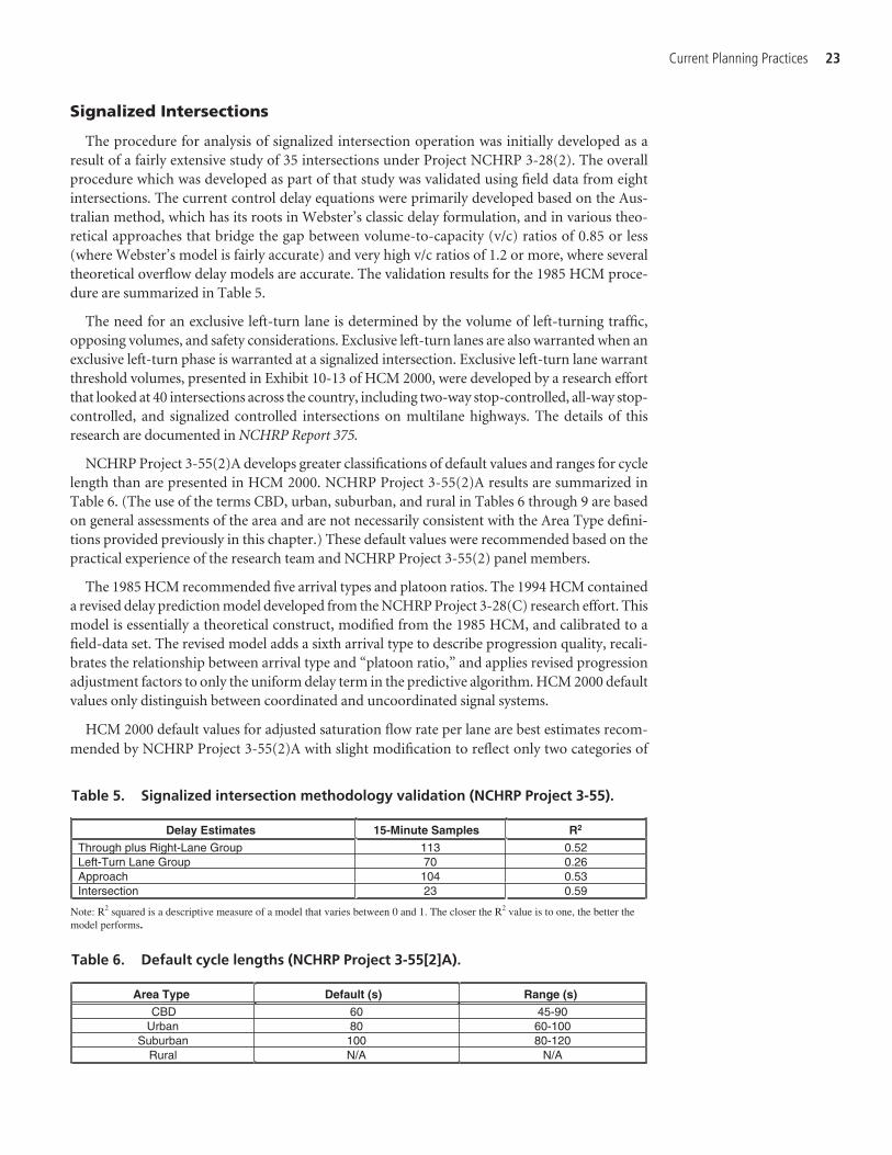
The procedure for analysis of signalized intersection operation was initially developed as aresult of a fairly extensive study of 35 intersections under Project NCHRP 3-28(2). The overallprocedure which was developed as part of that study was validated using field data from eightintersections. The current control delay equations were primarily developed based on the Aus-tralian method, which has its roots in Webster’s classic delay formulation, and in various theo-retical approaches that bridge the gap between volume-to-capacity (v/c) ratios of 0.85 or less(where Webster’s model is fairly accurate) and very high v/c ratios of 1.2 or more, where severaltheoretical overflow delay models are accurate. The validation results for the 1985 HCM proce-dure are summarized in Table 5.
The need for an exclusive left-turn lane is determined by the volume of left-turning traffic,opposing volumes, and safety considerations. Exclusive left-turn lanes are also warranted when anexclusive left-turn phase is warranted at a signalized intersection. Exclusive left-turn lane warrantthreshold volumes, presented in Exhibit 10-13 of HCM 2000, were developed by a research effortthat looked at 40 intersections across the country, including two-way stop-controlled, all-way stop-controlled, and signalized controlled intersections on multilane highways. The details of thisresearch are documented in NCHRP Report 375.
NCHRP Project 3-55(2)A develops greater classifications of default values and ranges for cyclelength than are presented in HCM 2000. NCHRP Project 3-55(2)A results are summarized inTable 6. (The use of the terms CBD, urban, suburban, and rural in Tables 6 through 9 are basedon general assessments of the area and are not necessarily consistent with the Area Type defini-tions provided previously in this chapter.) These default values were recommended based on thepractical experience of the research team and NCHRP Project 3-55(2) panel members.
The 1985 HCM recommended five arrival types and platoon ratios. The 1994 HCM containeda revised delay prediction model developed from the NCHRP Project 3-28(C) research effort. Thismodel is essentially a theoretical construct, modified from the 1985 HCM, and calibrated to afield-data set. The revised model adds a sixth arrival type to describe progression quality, recali-brates the relationship between arrival type and “platoon ratio,” and applies revised progressionadjustment factors to only the uniform delay term in the predictive algorithm. HCM 2000 defaultvalues only distinguish between coordinated and uncoordinated signal systems.
HCM 2000 default values for adjusted saturation flow rate per lane are best estimates recom-mended by NCHRP Project 3-55(2)A with slight modification to reflect only two categories of
Current Planning Practices 23
Table 5. Signalized intersection methodology validation (NCHRP Project 3-55).
Delay Estimates 15-Minute Samples R2
Through plus Right-Lane Group 113 0.52 Left-Turn Lane Group 70 0.26 Approach 104 0.53 Intersection 23 0.59
Note: R2 squared is a descriptive measure of a model that varies between 0 and 1. The closer the R2 value is to one, the better the model performs.
Table 6. Default cycle lengths (NCHRP Project 3-55[2]A).
Area Type Default (s) Range (s) CBD 60 45-90
Urban 80 60-100 Suburban 100 80-120
Rural N/A N/A
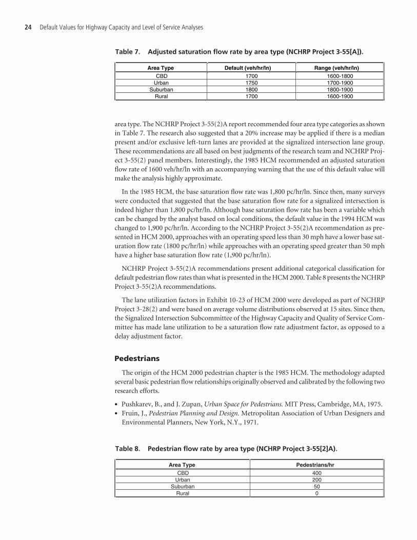
24 Default Values for Highway Capacity and Level of Service Analyses
Table 7. Adjusted saturation flow rate by area type (NCHRP Project 3-55[A]).
Area Type Default (veh/hr/ln) Range (veh/hr/ln) CBD 1700 1600-1800
Urban 1750 1700-1900 Suburban 1800 1800-1900
Rural 1700 1600-1900
Table 8. Pedestrian flow rate by area type (NCHRP Project 3-55[2]A).
Area Type Pedestrians/hrCBD 400
Urban 200 Suburban 50
Rural 0
area type. The NCHRP Project 3-55(2)A report recommended four area type categories as shownin Table 7. The research also suggested that a 20% increase may be applied if there is a medianpresent and/or exclusive left-turn lanes are provided at the signalized intersection lane group.These recommendations are all based on best judgments of the research team and NCHRP Proj-ect 3-55(2) panel members. Interestingly, the 1985 HCM recommended an adjusted saturationflow rate of 1600 veh/hr/ln with an accompanying warning that the use of this default value willmake the analysis highly approximate.
In the 1985 HCM, the base saturation flow rate was 1,800 pc/hr/ln. Since then, many surveyswere conducted that suggested that the base saturation flow rate for a signalized intersection isindeed higher than 1,800 pc/hr/ln. Although base saturation flow rate has been a variable whichcan be changed by the analyst based on local conditions, the default value in the 1994 HCM waschanged to 1,900 pc/hr/ln. According to the NCHRP Project 3-55(2)A recommendation as pre-sented in HCM 2000, approaches with an operating speed less than 30 mph have a lower base sat-uration flow rate (1800 pc/hr/ln) while approaches with an operating speed greater than 50 mphhave a higher base saturation flow rate (1,900 pc/hr/ln).
NCHRP Project 3-55(2)A recommendations present additional categorical classification fordefault pedestrian flow rates than what is presented in the HCM 2000. Table 8 presents the NCHRPProject 3-55(2)A recommendations.
The lane utilization factors in Exhibit 10-23 of HCM 2000 were developed as part of NCHRPProject 3-28(2) and were based on average volume distributions observed at 15 sites. Since then,the Signalized Intersection Subcommittee of the Highway Capacity and Quality of Service Com-mittee has made lane utilization to be a saturation flow rate adjustment factor, as opposed to adelay adjustment factor.
Pedestrians
The origin of the HCM 2000 pedestrian chapter is the 1985 HCM. The methodology adaptedseveral basic pedestrian flow relationships originally observed and calibrated by the following tworesearch efforts.
• Pushkarev, B., and J. Zupan, Urban Space for Pedestrians. MIT Press, Cambridge, MA, 1975.• Fruin, J., Pedestrian Planning and Design. Metropolitan Association of Urban Designers and
Environmental Planners, New York, N.Y., 1971.

Formulations for crosswalks and street corners were theoretical models based on time-spaceconcepts developed by Fruin. While basic relationships were calibrated to field data (all col-lected in New York City), crosswalk and street corner methodologies still have not been exten-sively validated. All of the pedestrian speed-density, flow-density, and speed-flow relationshipspresented in Chapter 11 of the HCM 2000 come from the Pushkarev and Zupan’s 1975research effort. Table 13-1 of the 1985 HCM presents walkway width, observed pedestrian flowrates compiled by Roger Roess and Herb Levinson from sites in Boston, Chicago, Los Ange-les, Des Moines and Ames, Iowa, New York City, Washington, D.C., Seattle, San Francisco,and Winnipeg.
The 1994 HCM recommends a pedestrian walking speed of 4.5 ft/s as the default value. Basedon the findings of an FHWA research project, “Recommended Procedures for Chapter 13, ‘Pedes-trians’ of The Highway Capacity Manual,” the walking speed default value was reduced to 4.0 ft/s.Greater emphasis was placed by this research on the importance of determining the proportion ofelderly pedestrians (65 years of age and older) in the walking population. Chapter 18 of HCM 2000recommends that if 0 to 20% of pedestrians are elderly, then a walking speed of 4.0 ft/s is appro-priate. If the elderly walking population exceeds 20%, then 3.3 ft/s is appropriate. In addition, anupgrade of 10% or greater reduces walking speed by 0.3 ft/s.
Field studies of pedestrians’ walking speed and start-up time were performed relative tosite and environmental factors, including street width, posted speed, curb height, grade,number of vehicle travel lanes, signal cycle length, pedestrian-signal type, street functionalclassification, crosswalk type, and channelization and were documented in TransportationResearch Record 1538: “Pedestrian and Bicycle Research.” Data were collected at sixteen cross-walks in four urban areas. The research recommended a default pedestrian walking speed of4.0 ft/s and a pedestrian start-up time of 3.0 s, which are essentially the same as the HCM 2000default values.
Bicycles
According to the AASHTO Policy on Geometric Design of Highways and Streets, on-street bicy-cle lane width should be a minimum of 5 ft. For short lengths of an off-street bicycle path or forconnectors, a minimum acceptable width is 8 ft. A 10-ft wide off-street bicycle path is the standard.The HCM 2000 default value for off-street bicycle path width is 8 ft for a two-lane path and 10 ftfor a three-lane path.
When using the HCM 2000 bicycle methodology, the analyst should keep in mind that bicycleflow peaking characteristics are very different from motor vehicles. Bicycle volumes peak moreabruptly. Daily volumes, or even hourly volumes, may not appear to be very substantial until thispeaking is considered. One study in Madison, Wisconsin, measured peak-hour volumes as 10 to15% of total daily volume at various locations. Another study in the State of Washington (con-ducted primarily in the Seattle area) measured PHFs of between 0.52 and 0.82 at various locations.Using these findings as a basis, the FHWA research “Recommended Procedures for Chapter 14,Bicycles of The Highway Capacity Manual” recommended a PHF of 0.80 as a default value inabsence of local data. This default was included in the HCM 2000.
A manual released by FHWA, “Safety and Locational Criteria for Bicycle Facilities, UserManual Volume II: Design and Safety Criteria,” reported that the 85th percentile speed ofbicycles is approximately 15 mph and that a design speed of 20 mph on level terrain wouldallow for nearly all bicyclists to travel at their desired speeds. Based on these findings, theFHWA research prior to the publication of HCM 2000—“Recommended Procedures forChapter 14, Bicycles of The Highway Capacity Manual”—recommended 15 mph as a defaultbicycle travel speed.
Current Planning Practices 25

Multilane Highways
The multilane highway procedure was developed prior to the publication of the 1985 HCMas part of NCHRP Project 3-33. The procedure was developed based on an extensive field studywhich covered some 47 sites across the United States. Over 530 15-minute samples were usedto establish the speed-flow relationship and analysis procedure. The multilane highway analy-sis procedure consists of two components used to estimate average travel speed and density.These components are flow rate and free-flow speed. In general, variation of lane width,median type, and access points per mile were found to account for 48% percent (R2 = 48) ofobserved variation in speed.
AASHTO design guidelines for multilane highways recommend a 12-ft lane width and 6-ftshoulder width. These values were included in the HCM 2000 as default values.
The access point density observed at the NCHRP Project 3-33 field sites was 11 access points/mi.However, access point density as high as 53 access points/mi was also found. Access points werenot differentiated between driveways or side streets. Only access points on the right-hand side ofthe travel way were considered. The NCHRP Project 3-33 findings are recommended as defaultvalues in the HCM 2000 (Exhibit 12-4).
The general terrain type can be used instead of specific grades whenever there is no single gradeon the highway segment that extends for more than 1 mi or the grade exceeds +/− 3% for morethan 0.5 mi. Even though “level” general terrain is recommended as the default value in the HCM2000, additional guidance is given in the HCM 2000. The directions described for selecting adefault general terrain are
• If average extended terrain is less than 3%, then use “Level Terrain,”• If average extended terrain is between 3 to 7%, then use “Rolling Terrain,” or• If average extended terrain is greater than 7%, then use “Mountainous Terrain.”
The base free-flow speed for multilane highways was defined by NCHRP Project 3-33 as theoperating speed under ideal roadway conditions, including 12-ft lane widths, a divided high-way with median, greater than 6-ft lateral clearance in both the median and the right side ofthe highway, and no access points. The recommended base free-flow speed for ideal condi-tions is 60 mph.
NCHRP Project 3-55(2)A suggests that the Highway Performance Monitoring System (HPMS)from the FHWA can be used to obtain local information on the percent of heavy vehicles by facil-ity and area type. If the breakdown between RVs, trucks, and buses is not known, then it is recom-mended that heavy vehicles be considered to be all trucks.
As part of NCHRP Project 3-33, driver population was surveyed informally during the fieldstudies. No definitive result was obtained concerning the operational effects of a commuter ver-sus recreational driver population. In all of the sites studied, commuter traffic (with in-statelicense plates) accounted for 90 to 95% of the total volume. The 1985 HCM, Chapter 3, Basic Free-way Sections methodology states that the driver population factor generally ranges from 0.75to 1.0. This factor is primarily based on California Department of Transportation (Caltrans)studies performed in the early 1970s on California freeways. Unfortunately, these traffic studiesperformed by Caltrans were internal working memos and are not currently available for review.A 1997 FHWA research project, Driver Population Factors in Freeway Capacity, collected severaldata sets across the State of Florida and determined that the HCM driver population factorsshould be in the range 0.85 to 1.0. Based on the Florida study results, the HCM 2000 recommendsthat if a significant portion of the driver population consists of recreational drivers, a populationfactor of 0.85 should be used.
26 Default Values for Highway Capacity and Level of Service Analyses
Two-Lane Highways
The original two-lane highway methodology was presented in the 1985 HCM. It was based ona complex set of algorithms developed using field data, data generated by a simulation model, andpublished results of foreign two-lane operations. The model was calibrated using limited field data.One aspect of the 1985 HCM procedure which was developed using field data was the passenger-car equivalencies for heavy vehicles on two-lane highways. Since then, NCHRP Project 3-55(3) col-lected traffic flow data at a total of 20 sites in four states and one Canadian province to improve thetwo-lane highway simulation TWOPAS, and develop a new procedure that is currently providedin Chapter 20 of the HCM 2000. The data collected at the 20 sites included traffic volumes, speed,platooning data on high-volume two-lane highways, comparison of speeds upstream and down-stream of shoulder width transitions on two-lane highways, truck crawl speeds on steep upgrades,and traffic operations on steep downgrades.
AASHTO design guidelines for two-lane highways in the United States recommend a 12-ft lanewidth and 6-ft shoulder width for high speed facilities. The HCM 2000 adopted these standardwidths as default values.
As part of NCHRP Project 3-55(2)A, Kittelson & Associates, Inc., surveyed 25 agencies acrossthe United States to identify default values of various HCM input parameters. Responses werereceived from 13 of the 25 agencies surveyed. The survey addressed various facility types, includ-ing arterials in CBDs, arterials in urban areas, suburban arterials, rural multilane highways, two-lane highways, CBD signalized intersections, urban signalized intersections, suburban signalizedintersections, CBD all-way stop-controlled intersections, urban all-way stop-controlled inter-sections, suburban all-way stopped intersections, and freeways. The default value recommendedin the HCM 2000 for percent no-passing zones was based on the survey results.
Basic Freeway Segments
The basic freeway segment procedure developed under NCHRP Project 3-45 is based primarilyon a large database (415 15-minute samples) representing 56 sites from across the United States.The recommended procedure consists of two components which are used to calculate travelspeed and density. The first component is the same analytical model that is used to estimatehourly flow rate in the 1985 procedure, accounting for the variability of flow between 15-minute periods (i.e., PHF) and the influence of heavy vehicles in the traffic stream combinedwith the effects of grade on heavy vehicle performance. Passenger-car equivalencies, which areused to describe the affect of heavy vehicles on traffic flow, were developed from several sources.The passenger-car equivalencies included in the 1985 HCM for freeways and multilane highwayswere generated using a model that simulated the operation of different vehicle types on spe-cific grades or terrains. The 1985 HCM included equivalencies representing three truck weight-to-horsepower classes and RVs. As part of the multilane highway research (NCHRP Project 3-33)heavy vehicles and RV equivalencies were updated using simulation and field data. The mini-mum equivalencies for trucks and RVs were developed from traffic flow data collected at twosites in California. In the 1994 HCM, the updated equivalencies were recommended for bothmultilane highways and freeways. Based on research conducted by Elefteriadou, lower heavyvehicle equivalencies were developed for HCM 2000.
The second component estimates the free-flow speed of the section based on roadway charac-teristics. Adjustments to a base free-flow speed are made for number of lanes, lane width, lateralclearance, and interchanges per mile. Although the research found no correlation between lanewidth and speed, the lane width adjustments developed from the multilane highway researchwere applied to freeways. The multilane highway research found a moderate correlation betweenlane width and speed.
Current Planning Practices 27

NCHRP Project 3-45 also looked at variation in the basic freeway segment speed-flow relation-ship between four metropolitan areas where data were collected. Four cities (San Diego, Sacra-mento, Seattle, and Des Moines) were compared. Statistical analysis of the data indicated that sitelocation accounted for 42% of the variation in speed. Free-flow speeds observed at the four sitesranged from 58 to 65 mph. Although the comparison of traffic flow data was limited to four cities,the research suggested that this variation in the speed-flow relationship was due to a broad rangeof factors, including driver aggressiveness and level of enforcement.
AASHTO design guidelines for freeways in the Untied States are 12-ft lane width and 10-ftright-shoulder width. These recommendations were included in the HCM 2000 as default values.
NCHRP Project 3-45 recommended a 70-mph base free-flow speed for all types of freeways.After the national speed limit was raised, a 75-mph free-flow speed curve was added. The HCM2000 recommends a 75-mph base free-flow speed for rural freeways and a 70-mph free-flowspeed for urban freeways.
Ramps and Ramp Junctions
The 1994 HCM procedures for the analysis of freeway-ramp merge and diverge areas were devel-oped by NCHRP Project 3-37. This research involved a rather extensive field study of some 68 sitesin 10 states, generating 341 15-minute samples. The procedure consists of essentially two compo-nents: estimation of the volume in lanes 1 and 2 of the freeway and estimation of the average speedand density of traffic within the merge or diverge influence areas. A series of equations to esti-mate the volumes in the two lanes immediately adjacent to the ramp (lanes 1 and 2) were devel-oped empirically for both merge and diverge influence areas. The equations were based on a con-sistently strong correlation between volume in lanes 1 and 2 with total freeway volume, regardlessof the number of lanes. Depending upon the number of lanes and presence of upstream or down-stream ramps, a predictive model was calibrated using field data. NCHRP Project 3-55(6) added aspeed prediction model for the outside lanes of the freeway.
NCHRP Project 3-55(2)A included a broader range of acceleration and deceleration lane lengthsthan what is presented in the HCM 2000. The NCHRP Project 3-55(2) recommendations are pro-vided in Table 9. These default values were calculated using AASHTO design standards for a 12-ftwide single-lane ramp, the tangent angle for exit ramps which ranges from 2 to 5%, and the taperrate for entry ramps which ranges from 50:1 to 60:1.
Transit
The transit variables, current defaults, and those input parameters that have the greatest impacton the results are provided in Table 10. Despite the absence of transit default values in the HCM2000, the TCQSM provides default values for a number of variables. The TCQSM has gone throughseveral updates since the publication of HCM 2000. Other transit-related default values in theHCM 2000 were recommended based on vast experience of transit operators and TCRP researchagencies.
28 Default Values for Highway Capacity and Level of Service Analyses
Table 9. Freeway ramps acceleration/deceleration lane lengths (NCHRP Project 3-55[2]A).
Area Type Length of Acceleration Lanes (ft) Length of Deceleration Lanes (ft)CBD 650 165 Urban 650 165 Suburban 750 250 Rural 825 325
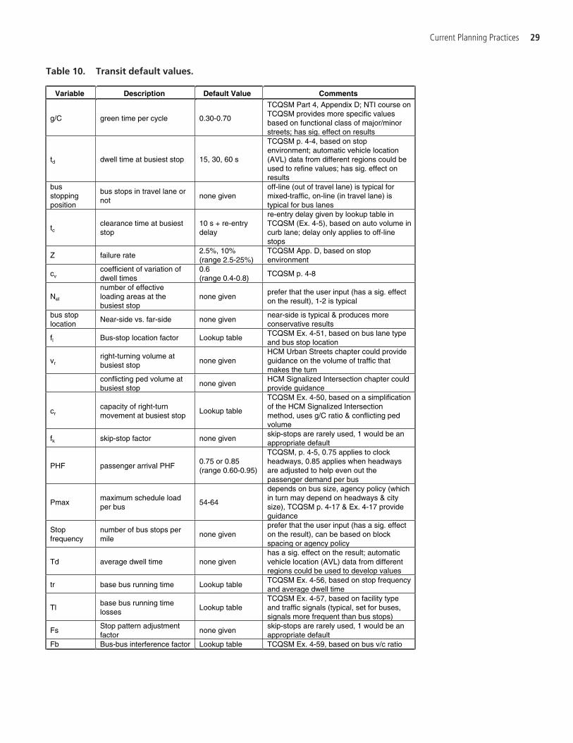
Current Planning Practices 29
Table 10. Transit default values.
Variable Description Default Value Comments
g/C green time per cycle 0.30-0.70
TCQSM Part 4, Appendix D; NTI course on TCQSM provides more specific values based on functional class of major/minor streets; has sig. effect on results
td dwell time at busiest stop 15, 30, 60 s
TCQSM p. 4-4, based on stop environment; automatic vehicle location (AVL) data from different regions could be used to refine values; has sig. effect onresults
busstoppingposition
bus stops in travel lane ornot
none given off-line (out of travel lane) is typical for mixed-traffic, on-line (in travel lane) istypical for bus lanes
tcclearance time at busiest stop
10 s + re-entry delay
re-entry delay given by lookup table in TCQSM (Ex. 4-5), based on auto volume in curb lane; delay only applies to off-line stops
Z failure rate 2.5%, 10% (range 2.5-25%)
TCQSM App. D, based on stop environment
cvcoefficient of variation ofdwell times
0.6(range 0.4-0.8)
TCQSM p. 4-8
Nel
number of effectiveloading areas at the busiest stop
none given prefer that the user input (has a sig. effecton the result), 1-2 is typical
bus stop location
Near-side vs. far-side none given near-side is typical & produces more conservative results
fl Bus-stop location factor Lookup table TCQSM Ex. 4-51, based on bus lane type and bus stop location
vrright-turning volume at busiest stop
none given HCM Urban Streets chapter could provide guidance on the volume of traffic that makes the turn
conflicting ped volume atbusiest stop
none given HCM Signalized Intersection chapter could provide guidance
crcapacity of right-turn movement at busiest stop
Lookup table
TCQSM Ex. 4-50, based on a simplification of the HCM Signalized Intersection method, uses g/C ratio & conflicting ped volume
fk skip-stop factor none given skip-stops are rarely used, 1 would be an appropriate default
PHF passenger arrival PHF 0.75 or 0.85 (range 0.60-0.95)
TCQSM, p. 4-5, 0.75 applies to clock headways, 0.85 applies when headways are adjusted to help even out the passenger demand per bus
Pmaxmaximum schedule load per bus
54-64
depends on bus size, agency policy (which in turn may depend on headways & citysize), TCQSM p. 4-17 & Ex. 4-17 provide guidance
Stop frequency
number of bus stops per mile
none given prefer that the user input (has a sig. effect on the result), can be based on blockspacing or agency policy
Td average dwell time none given has a sig. effect on the result; automatic vehicle location (AVL) data from different regions could be used to develop values
tr base bus running time Lookup table TCQSM Ex. 4-56, based on stop frequency and average dwell time
Tlbase bus running time losses
Lookup tableTCQSM Ex. 4-57, based on facility type and traffic signals (typical, set for buses,signals more frequent than bus stops)
FsStop pattern adjustment factor
none given skip-stops are rarely used, 1 would be an appropriate default
Fb Bus-bus interference factor Lookup table TCQSM Ex. 4-59, based on bus v/c ratio
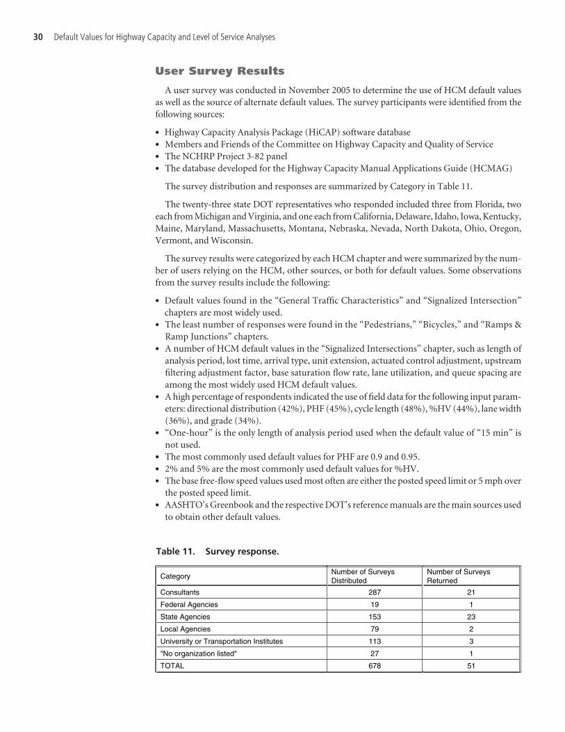
User Survey Results
A user survey was conducted in November 2005 to determine the use of HCM default valuesas well as the source of alternate default values. The survey participants were identified from thefollowing sources:
• Highway Capacity Analysis Package (HiCAP) software database• Members and Friends of the Committee on Highway Capacity and Quality of Service• The NCHRP Project 3-82 panel• The database developed for the Highway Capacity Manual Applications Guide (HCMAG)
The survey distribution and responses are summarized by Category in Table 11.
The twenty-three state DOT representatives who responded included three from Florida, twoeach from Michigan and Virginia, and one each from California, Delaware, Idaho, Iowa, Kentucky,Maine, Maryland, Massachusetts, Montana, Nebraska, Nevada, North Dakota, Ohio, Oregon,Vermont, and Wisconsin.
The survey results were categorized by each HCM chapter and were summarized by the num-ber of users relying on the HCM, other sources, or both for default values. Some observationsfrom the survey results include the following:
• Default values found in the “General Traffic Characteristics” and “Signalized Intersection”chapters are most widely used.
• The least number of responses were found in the “Pedestrians,” “Bicycles,” and “Ramps &Ramp Junctions” chapters.
• A number of HCM default values in the “Signalized Intersections” chapter, such as length ofanalysis period, lost time, arrival type, unit extension, actuated control adjustment, upstreamfiltering adjustment factor, base saturation flow rate, lane utilization, and queue spacing areamong the most widely used HCM default values.
• A high percentage of respondents indicated the use of field data for the following input param-eters: directional distribution (42%), PHF (45%), cycle length (48%), %HV (44%), lane width(36%), and grade (34%).
• “One-hour” is the only length of analysis period used when the default value of “15 min” isnot used.
• The most commonly used default values for PHF are 0.9 and 0.95.• 2% and 5% are the most commonly used default values for %HV.• The base free-flow speed values used most often are either the posted speed limit or 5 mph over
the posted speed limit.• AASHTO’s Greenbook and the respective DOT’s reference manuals are the main sources used
to obtain other default values.
30 Default Values for Highway Capacity and Level of Service Analyses
Table 11. Survey response.
CategoryNumber of Surveys Distributed
Number of Surveys Returned
Consultants 287 21
Federal Agencies 19 1
State Agencies 153 23
Local Agencies 79 2
University or Transportation Institutes 113 3
"No organization listed" 27 1
TOTAL 678 51
Approximately one-third of the input parameters with an associated HCM default value havea significant impact on the point or facility service measure. In general, input parameters thatdescribe the facility type, area type, terrain type, and geometric configuration (such as lane width,segment length, and interchange spacing) are readily available to the analyst. Default values shouldnot be used for these input parameters. The remaining input parameters that are highly sensitivecan be broken into two categories:
• Data can be obtained and the default value may be confirmed, updated, or defined further asa function of a range of variables such as region, city size, volume, and so forth. This chapteraddresses these input parameters.
• Data are not readily available; however, guidance regarding the selection of an appropriatedefault value can be provided based on research contained in the literature. Chapter 4 addressesthese input parameters.
The input parameters that have a significant impact on the service measure are summa-rized in Table 12. For each of these input parameters, either a revised set of default values isrecommended (in Chapter 3) or guidance on the selection of appropriate input parametersis provided (in Chapter 4). Some input parameters that did not have a high degree of sensi-tivity are also addressed.
In addition to these input parameters, PHF and %HV were investigated for all uninterruptedand interrupted facilities. Despite low to moderate sensitivity results for two-lane and multilanehighways, this type of data is readily available and the existing defaults were explored further.Although there are no default values provided for unsignalized intersections in HCM 2000, PHFand %HV were investigated for unsignalized intersections due to the impact that these inputparameters could have on the level of service measure.
Defining Default Values by Category
As a result of insufficient field data, the HCM recommends that only a single default value beused for many key input parameters. Thus, the variation of traffic and geometric conditionsacross the United States is not considered. Each input parameter could potentially be describedby environmental variables, such as metropolitan size or geographic region, to determine ifdriver behavior or local design practices impact the magnitude of the input parameter. There areeight independent variables that have been examined in the development of default values. Theseindependent variables are categorized as global and non-global variables and are shown belowin Table 13.
31
C H A P T E R 3
Recommended Default Values
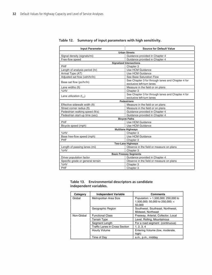
32 Default Values for Highway Capacity and Level of Service Analyses
Input Parameter Source for Default Value Urban Streets
Signal density (signals/mi) Guidance provided in Chapter 4 Free-flow speed Guidance provided in Chapter 4
Signalized Intersections PHF Chapter 3 Length of analysis period (hr) Use HCM Guidance Arrival Type (AT) Use HCM Guidance Adjusted sat flow (veh/hr/ln) See Base Saturation Flow
Base sat flow (pc/hr/ln) See Chapter 3 for through lanes and Chapter 4 for exclusive left-turn lanes
Lane widths (ft) Measure in the field or on plans %HV Chapter 3
Lane utilization (fLU) See Chapter 3 for through lanes and Chapter 4 for exclusive left-turn lanes
Pedestrians Effective sidewalk width (ft) Measure in the field or on plans Street corner radius (ft) Measure in the field or on plans Pedestrian walking speed (ft/s) Guidance provided in Chapter 4 Pedestrian start-up time (sec) Guidance provided in Chapter 4
Bicycle Paths PHF Use HCM Guidance Bicycle speed (mph) Use HCM Guidance
Multilane Highways %HV Chapter 3 Base free-flow speed (mph) Use HCM Guidance PHF Chapter 3
Two-Lane Highways Length of passing lanes (mi) Observe in the field or measure on plans %HV Chapter 3
Basic Freeway Segments Driver population factor Guidance provided in Chapter 4 Specific grade or general terrain Observe in the field or measure on plans %HV Chapter 3 PHF Chapter 3
Table 12. Summary of input parameters with high sensitivity.
Category Independent Variable Comments Metropolitan Area Size Population: > 1,500,000; 250,000 to
1,500,000; 50,000 to 250,000; < 50,000
Global
Geographic Region Southwest, Southeast, Northwest,Midwest, Northeast
Functional Class Freeway, Arterial, Collector, Local Terrain Type Level, Rolling, MountainousSegment Length For a road segment (continuous)Traffic Lanes in Cross Section 1, 2, 3, 4 Hourly Volume Entering Volume (low, moderate,
high)
Non-Global
Time of Day a.m., p.m., midday
Table 13. Environmental descriptors as candidate independent variables.
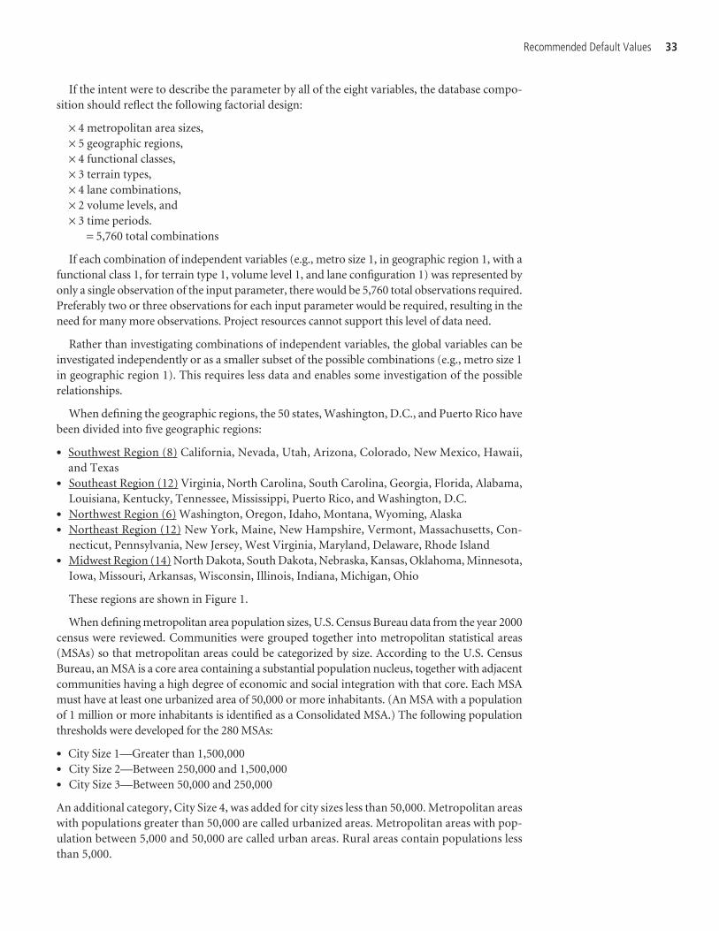
If the intent were to describe the parameter by all of the eight variables, the database compo-sition should reflect the following factorial design:
× 4 metropolitan area sizes,× 5 geographic regions,× 4 functional classes,× 3 terrain types,× 4 lane combinations,× 2 volume levels, and× 3 time periods.
= 5,760 total combinations
If each combination of independent variables (e.g., metro size 1, in geographic region 1, with afunctional class 1, for terrain type 1, volume level 1, and lane configuration 1) was represented byonly a single observation of the input parameter, there would be 5,760 total observations required.Preferably two or three observations for each input parameter would be required, resulting in theneed for many more observations. Project resources cannot support this level of data need.
Rather than investigating combinations of independent variables, the global variables can beinvestigated independently or as a smaller subset of the possible combinations (e.g., metro size 1in geographic region 1). This requires less data and enables some investigation of the possiblerelationships.
When defining the geographic regions, the 50 states, Washington, D.C., and Puerto Rico havebeen divided into five geographic regions:
• Southwest Region (8) California, Nevada, Utah, Arizona, Colorado, New Mexico, Hawaii,and Texas
• Southeast Region (12) Virginia, North Carolina, South Carolina, Georgia, Florida, Alabama,Louisiana, Kentucky, Tennessee, Mississippi, Puerto Rico, and Washington, D.C.
• Northwest Region (6) Washington, Oregon, Idaho, Montana, Wyoming, Alaska• Northeast Region (12) New York, Maine, New Hampshire, Vermont, Massachusetts, Con-
necticut, Pennsylvania, New Jersey, West Virginia, Maryland, Delaware, Rhode Island• Midwest Region (14) North Dakota, South Dakota, Nebraska, Kansas, Oklahoma, Minnesota,
Iowa, Missouri, Arkansas, Wisconsin, Illinois, Indiana, Michigan, Ohio
These regions are shown in Figure 1.
When defining metropolitan area population sizes, U.S. Census Bureau data from the year 2000census were reviewed. Communities were grouped together into metropolitan statistical areas(MSAs) so that metropolitan areas could be categorized by size. According to the U.S. CensusBureau, an MSA is a core area containing a substantial population nucleus, together with adjacentcommunities having a high degree of economic and social integration with that core. Each MSAmust have at least one urbanized area of 50,000 or more inhabitants. (An MSA with a populationof 1 million or more inhabitants is identified as a Consolidated MSA.) The following populationthresholds were developed for the 280 MSAs:
• City Size 1—Greater than 1,500,000• City Size 2—Between 250,000 and 1,500,000• City Size 3—Between 50,000 and 250,000
An additional category, City Size 4, was added for city sizes less than 50,000. Metropolitan areaswith populations greater than 50,000 are called urbanized areas. Metropolitan areas with pop-ulation between 5,000 and 50,000 are called urban areas. Rural areas contain populations lessthan 5,000.
Recommended Default Values 33

Data Sources and Calculation Methodology
Sources for input parameter data were obtained from the following three categories:
1. Completed (or ongoing) research projects—NCHRP, FHWA, and state research efforts aswell as published reports.
2. Governmental Agencies—Database sources in the governmental agency category includedvarious count programs from federal, state, county, and city agencies.
3. “In-house” databases assembled from transportation projects.
Two types of data can be collected: explicit default values and raw data. Explicit default valuesare default values found in city, county, state, or federal sources that have been previously definedbased on raw data. Raw data statistics are used to compute a mean default value for each “site.” A“site” is defined as an individual traffic movement served by the facility and for which a level ofservice can be computed using a methodology in the HCM.
A number of the default values have a basis that includes a temporal representation. Thesevariables represent a traffic characteristic that includes the count of vehicles for a given unit oftime (e.g., volume). In these instances, the basis for the variable is defined to be the time periodthat is associated with the peak hour of the average week day (PAW), where the peak hour isdefined using the flow rate of vehicular traffic. Other time periods may be used as the basis forcomputation if the data in these alternative time periods are determined to be representative ofthe PAW. The peak hour (and in some cases the peak 15-min period) is recommended as thebasis for defining default values because this time period is most commonly used for capacityand level-of-service analysis.
34 Default Values for Highway Capacity and Level of Service Analyses
Figure 1. Geographic region boundaries.
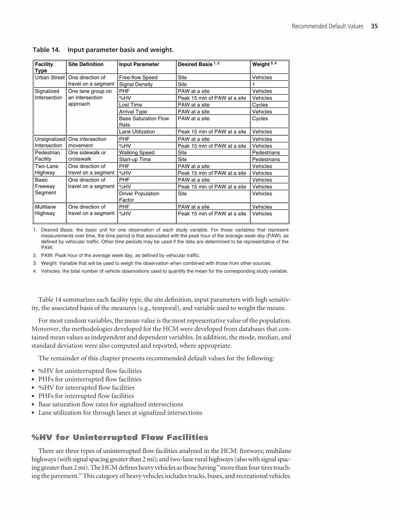
Table 14 summarizes each facility type, the site definition, input parameters with high sensitiv-ity, the associated basis of the measures (e.g., temporal), and variable used to weight the means.
For most random variables, the mean value is the most representative value of the population.Moreover, the methodologies developed for the HCM were developed from databases that con-tained mean values as independent and dependent variables. In addition, the mode, median, andstandard deviation were also computed and reported, where appropriate.
The remainder of this chapter presents recommended default values for the following:
• %HV for uninterrupted flow facilities• PHFs for uninterrupted flow facilities• %HV for interrupted flow facilities• PHFs for interrupted flow facilities• Base saturation flow rates for signalized intersections• Lane utilization for through lanes at signalized intersections
%HV for Uninterrupted Flow Facilities
There are three types of uninterrupted flow facilities analyzed in the HCM: freeways; multilanehighways (with signal spacing greater than 2 mi); and two-lane rural highways (also with signal spac-ing greater than 2 mi). The HCM defines heavy vehicles as those having “more than four tires touch-ing the pavement.” This category of heavy vehicles includes trucks, buses, and recreational vehicles.
Recommended Default Values 35
FacilityType
Site Definition Input Parameter Desired Basis 1, 2 Weight 3, 4
Free-flow Speed Site Vehicles Urban Street One direction of travel on a segment Signal Density Site 1
PHF PAW at a site Vehicles %HV Peak 15 min of PAW at a site Vehicles Lost Time PAW at a site Cycles Arrival Type PAW at a site Vehicles Base Saturation Flow Rate
PAW at a site Cycles
SignalizedIntersection
One lane group on an intersection approach
Lane Utilization Peak 15 min of PAW at a site Vehicles PHF PAW at a site Vehicles Unsignalized
IntersectionOne intersection movement %HV Peak 15 min of PAW at a site Vehicles
Walking Speed Site PedestriansPedestrianFacility
One sidewalk orcrosswalk Start-up Time Site Pedestrians
PHF PAW at a site Vehicles Two-Lane Highway
One direction oftravel on a segment %HV Peak 15 min of PAW at a site Vehicles
PHF PAW at a site Vehicles %HV Peak 15 min of PAW at a site Vehicles
BasicFreewaySegment
One direction oftravel on a segment
Driver Population Factor
Site Vehicles
PHF PAW at a site Vehicles MultilaneHighway
One direction oftravel on a segment %HV Peak 15 min of PAW at a site Vehicles
1. Desired Basis: the basic unit for one observation of each study variable. For those variables that represent measurements over time, the time period is that associated with the peak hour of the average week day (PAW), as defined by vehicular traffic. Other time periods may be used if the data are determined to be representative of the PAW.
2. PAW: Peak hour of the average week day, as defined by vehicular traffic.
3. Weight: Variable that will be used to weigh the observation when combined with those from other sources.
4. Vehicles: the total number of vehicle observations used to quantify the mean for the corresponding study variable.
Table 14. Input parameter basis and weight.
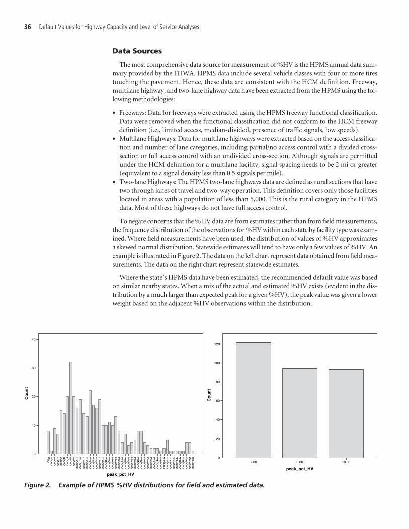
Data Sources
The most comprehensive data source for measurement of %HV is the HPMS annual data sum-mary provided by the FHWA. HPMS data include several vehicle classes with four or more tirestouching the pavement. Hence, these data are consistent with the HCM definition. Freeway,multilane highway, and two-lane highway data have been extracted from the HPMS using the fol-lowing methodologies:
• Freeways: Data for freeways were extracted using the HPMS freeway functional classification.Data were removed when the functional classification did not conform to the HCM freewaydefinition (i.e., limited access, median-divided, presence of traffic signals, low speeds).
• Multilane Highways: Data for multilane highways were extracted based on the access classifica-tion and number of lane categories, including partial/no access control with a divided cross-section or full access control with an undivided cross-section. Although signals are permittedunder the HCM definition for a multilane facility, signal spacing needs to be 2 mi or greater(equivalent to a signal density less than 0.5 signals per mile).
• Two-lane Highways: The HPMS two-lane highways data are defined as rural sections that havetwo through lanes of travel and two-way operation. This definition covers only those facilitieslocated in areas with a population of less than 5,000. This is the rural category in the HPMSdata. Most of these highways do not have full access control.
To negate concerns that the %HV data are from estimates rather than from field measurements,the frequency distribution of the observations for %HV within each state by facility type was exam-ined. Where field measurements have been used, the distribution of values of %HV approximatesa skewed normal distribution. Statewide estimates will tend to have only a few values of %HV. Anexample is illustrated in Figure 2. The data on the left chart represent data obtained from field mea-surements. The data on the right chart represent statewide estimates.
Where the state’s HPMS data have been estimated, the recommended default value was basedon similar nearby states. When a mix of the actual and estimated %HV exists (evident in the dis-tribution by a much larger than expected peak for a given %HV), the peak value was given a lowerweight based on the adjacent %HV observations within the distribution.
36 Default Values for Highway Capacity and Level of Service Analyses
57.00
56.00
54.00
49.00
48.00
47.00
46.00
45.00
41.00
40.00
39.00
37.00
34.00
33.00
32.00
31.00
30.00
29.00
28.00
27.00
26.00
25.00
24.00
23.00
22.00
21.00
20.00
19.00
18.00
17.00
16.00
15.00
14.00
13.00
12.00
11.00
10.00
9.00
8.00
7.00
6.00
5.00
4.00
3.00
1.00
.00
peak_pct_HV
40
30
20
10
0
Co
un
t
10.008.007.00
peak_pct_HV
120
100
80
60
40
20
0
Co
un
t
Figure 2. Example of HPMS %HV distributions for field and estimated data.

The data were also checked to confirm that the same values were not reported for both the peakperiod and the daily %HV. The difference between the two values was calculated. A zero differencewas observed for Missouri, Montana, Nevada, North Carolina, South Dakota, Utah, and Wyoming.Zero differences were also observed for some road types in Idaho, Iowa, North Dakota, andLouisiana. Most of these states are rural in character without large urban areas. Further, all fournon-freeway road types (and two freeway categories) are rural or are present in small urban areas.In these areas, peaking will not be very severe. Default values for these states were produced froma combination of their daily average %HV data and information on the average difference betweenpeak period and average daily %HV for similar and/or nearby states in the HPMS database.
The data underlying the recommended default values were obtained from the Year 2004 HPMSdatabase, the latest available at the time data collection for this project was undertaken. These val-ues are reasonable for use in the intermediate-term future. If external conditions change, it maymake sense to vary the default values from those that are provided here. For example, if gasolinebecomes so expensive that auto drivers reduce their use of private cars, the %HV reported heremay increase. In the absence of any major change, state and local agencies may wish to conduct asimple statistical analysis of their own HPMS data submissions every 5 years to determine if therehas been a change in %HV.
Data Summary and Analysis
The HPMS data contain information on the state and population category for each section ofroadway. Some states have a very large number of observations for a particular category, whileother states have very few observations. Because of the size of this database, it is possible to teststatistically whether regionalization is appropriate for %HV. Based on the analysis, statisticallysignificant differences were observed in the mean peak period %HV among the states within eachregion and facility type. Given the consistent results of these analyses, the default values have beenpresented at the state level, rather than for each of the five geographic regions.
Recommended Default Values
Table 15 reports the mean peak period %HV by state for two-lane and multilane highways thatoccur within the lowest two population categories. The mean values in the table are presented tothe nearest integer, since that is the level of precision of the data in the HPMS. Note that the meanvalues in this table represent averages over a wide range of actual observed values of %HV. Inmany instances, an analyst could develop a more refined value of %HV by considering such thingsas surrounding land uses (for example factories or warehouses at one extreme; solely residentialat another).
Table 16 reports the mean, standard deviation, and number of observations for the peak period%HV on freeways in four population categories. All values in the table are presented to the near-est integer, since that is the level of precision of the data in the HPMS. In general, the mean valueof %HV is the recommended default value in the absence of any other information. But, usersare urged to consider the magnitude of the standard deviation as an indication of the spread ofthe data. Changes to the mean values can be considered based on knowledge of local conditions.
PHFs for Uninterrupted Flow Facilities
The HCM defines PHF as “a measure of traffic demand fluctuation within the peak hour”which can be computed by dividing the peak hourly volume by the hourly equivalent of the peak15-min flow rate within that peak hour. For the uninterrupted flow data, PHFs were calculated
Recommended Default Values 37
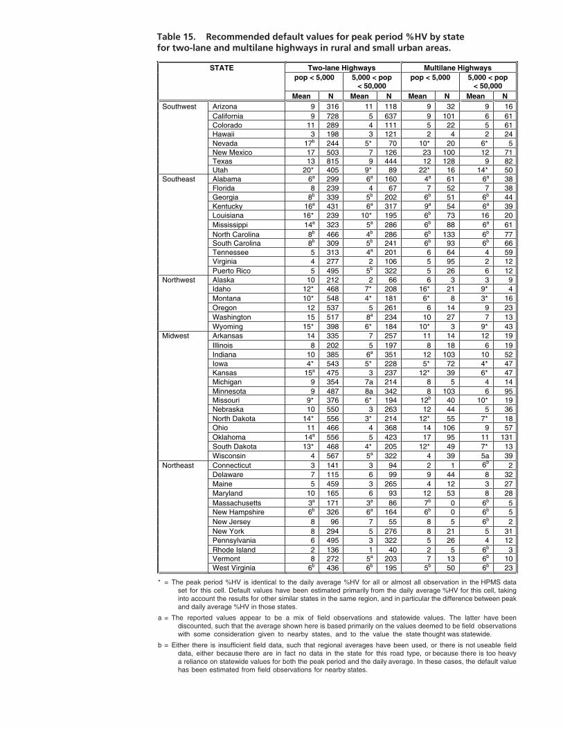
Two-lane Highways Multilane Highwayspop < 5,000 5,000 < pop
< 50,000pop < 5,000 5,000 < pop
< 50,000
STATE
Mean N Mean N Mean N Mean NArizona 9 316 11 118 9 32 9 16California 9 728 5 637 9 101 6 61Colorado 11 289 4 111 5 22 5 61Hawaii 3 198 3 121 2 4 2 24Nevada 17b 244 5* 70 10* 20 6* 5New Mexico 17 503 7 126 23 100 12 71Texas 13 815 9 444 12 128 9 82
Southwest
Utah 20* 405 9* 89 22* 16 14* 50Alabama 6a 299 6a 160 4a 61 6a 38Florida 8 239 4 67 7 52 7 38Georgia 8b 339 5b 202 6b 51 6b 44Kentucky 16a 431 6a 317 9a 54 6a 39Louisiana 16* 239 10* 195 6b 73 16 20Mississippi 14a 323 5a 286 6b 88 6a 61North Carolina 8b 466 4b 286 6b 133 6b 77South Carolina 8b 309 5b 241 6b 93 6b 66Tennessee 5 313 4a 201 6 64 4 59Virginia 4 277 2 106 5 95 2 12
Southeast
Puerto Rico 5 495 5b 322 5 26 6 12Alaska 10 212 2 66 6 3 3 9Idaho 12* 468 7* 208 16* 21 9* 4Montana 10* 548 4* 181 6* 8 3* 16Oregon 12 537 5 261 6 14 9 23Washington 15 517 8a 234 10 27 7 13
Northwest
Wyoming 15* 398 6* 184 10* 3 9* 43Arkansas 14 335 7 257 11 14 12 19Illinois 8 202 5 197 8 18 6 19Indiana 10 385 6a 351 12 103 10 52Iowa 4* 543 5* 228 5* 72 4* 47Kansas 15a 475 3 237 12* 39 6* 47Michigan 9 354 7a 214 8 5 4 14Minnesota 9 487 8a 342 8 103 6 95Missouri 9* 376 6* 194 12b 40 10* 19Nebraska 10 550 3 263 12 44 5 36North Dakota 14* 556 3* 214 12* 55 7* 18Ohio 11 466 4 368 14 106 9 57Oklahoma 14a 556 5 423 17 95 11 131South Dakota 13* 468 4* 205 12* 49 7* 13
Midwest
Wisconsin 4 567 5a 322 4 39 5a 39Connecticut 3 141 3 94 2 1 6b 2Delaware 7 115 6 99 9 44 8 32Maine 5 459 3 265 4 12 3 27Maryland 10 165 6 93 12 53 8 28Massachusetts 3a 171 3a 86 7b 0 6b 5New Hampshire 6b 326 6a 164 6b 0 6b 5New Jersey 8 96 7 55 8 5 6b 2New York 8 294 5 276 8 21 5 31Pennsylvania 6 495 3 322 5 26 4 12Rhode Island 2 136 1 40 2 5 6b 3Vermont 8 272 5a 203 7 13 6b 10
Northeast
West Virginia 6b 436 6b 195 5b 50 6b 23
* = The peak period %HV is identical to the daily average %HV for all or almost all observation in the HPMS data set for this cell. Default values have been estimated primarily from the daily average %HV for this cell, taking into account the results for other similar states in the same region, and in particular the difference between peak and daily average %HV in those states.
a = The reported values appear to be a mix of field observations and statewide values. The latter have been discounted, such that the average shown here is based primarily on the values deemed to be field observations with some consideration given to nearby states, and to the value the state thought was statewide.
b = Either there is insufficient field data, such that regional averages have been used, or there is not useable field data, either because there are in fact no data in the state for this road type, or because there is too heavy a reliance on statewide values for both the peak period and the daily average. In these cases, the default value has been estimated from field observations for nearby states.
Table 15. Recommended default values for peak period %HV by state for two-lane and multilane highways in rural and small urban areas.
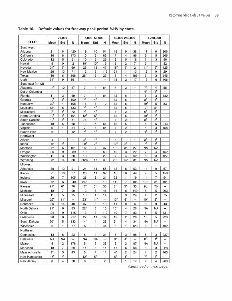
Recommended Default Values 39
<5,000 5,000- 50,000 50,000-250,000 >250,000STATE Mean Std N Mean Std N Mean Std N Mean Std N
Southwest Arizona 21 8 420 19 10 51 18 9 38 11 6 206 California 16 8 173 10 6 86 7 4 86 6 5 566 Colorado 12 5 51 10 5 26 8 5 18 7 3 96 Hawaii 5 0 2 19b 10b 16 2 2 7 3 1 32 Nevada 34b 9b 69 26 13 47 18b 9b 2 11b 6b 125 New Mexico 26 13 71 12 6 119 21 11 13 12 9 29 Texas 16 8 168 28* 6 23 8 4 186 5 3 545 Utah 34* 9 161 -- -- -- 18 2 17 13 6 106 Southeast (1), (2) Alabama 14a 10 47 7 4 84 7 2 -- 7a 4 58 Dst of Columbia -- -- -- -- -- -- -- -- -- 4b 3b -- Florida 11 3 69 7 4 84 12 6 -- 6 3 330 Georgia 19b 5b 100 7b 4b -- 12 6 -- 8b 5b -- Kentucky 20a 4 108 16 6 10 12 6 -- 10a 5 83 Louisiana 12* 6 133 7b 4b -- 12 6 -- 10* 5* -- Mississippi 9b 3b 72 7b 4b -- 7 2 -- 6b 3b -- North Carolina 19b 5b 104 12b 6b -- 12 6 -- 10a 5b -- South Carolina 19b 5b 81 7b 4b -- 7 2 -- 8b 5b -- Tennessee 19 5 68 12 6 61 12 6 -- 8 5 243 Virginia 9 4 54 7 4 84 7 2 -- 4 3 158 Puerto Rico 6 1 12 7b 4b -- 7 2 -- 4b 3b -- NorthwestAlaska 4 -- 1 5b 1b -- 5 -- 1 3b 1b -- Idaho 29* 6b -- 28b 7b -- 12b 3b -- 7b 4b -- Montana 22* 6 161 16* 7 37 12* 3* 27 NA NA -- Oregon 26 9 289 19 9 60 10 3 22 7 4 152 Washington 11 3 60 10 2 22 7 4 62 6 3 127 Wyoming 33* 14 88 36*a 17 39 28* 14* 31 NA NA --
MidwestArkansas 30 12 91 24 14 55 13 8 53 14 9 67
Illinois 21 10 87 23 11 32 16 6 44 9 5 158
Indiana 26 7 105 25 6 21 23 11 19 14 7 94 Iowa 20* 6 240 24* 2 19 11* 7 105 10* 8* 101
Kansas 21* 8* 78 17* 5* 36 8* 3* 35 9b 7b --
Michigan 18 7 90 12 8 48 13 8 140 8 5 263 Minnesota 11 5 75 10 4 14 6 3 24 4 2 75
Missouri 29b 11b -- 23b 11b -- 13b 6b -- 10b 5b --
Nebraska 36 14 48 37 6 10 11 0 6 8 9 43 North Dakota 21* 6 83 22* 3 10 10* 4 26 NA NA --
Ohio 24 9 115 13 7 112 10 7 83 8 5 431
Oklahoma 28 8 217 27 11 105 12 2 20 10 5 228 South Dakota 20* 5 133 14* 4 25 9* 4 34 NA NA --
Wisconsin 6 1 77 6 2 44 6 1 123 6 1 102
NortheastConnecticut 13 6 23 6 4 31 6 3 98 5 3 237
Delaware NA NA -- NA NA -- 9b 4b -- 8b 4b --
Maine 5 2 178 5 2 36 5 2 87 NA NA -- Maryland 18 7 69 14 5 11 17 6 66 8 3 228
Massachusetts 7a 5 43 5 4 11 4a 2 24 4 2 463
New Hampshire 15b 7b -- 12b 5b -- 6b 1b -- 7b 3b -- New Jersey 8 4 38 6 0 2 6 1 17 9 4 268
Table 16. Default values for freeway peak period %HV by state.
(continued on next page)
40 Default Values for Highway Capacity and Level of Service Analyses
<5,000 5,000- 50,000 50,000-250,000 >250,000STATE Mean Std N Mean Std N Mean Std N Mean Std N
New York 18 5 106 11 4 83 11 4 114 7 4 269
Pennsylvania 16 6 1859 13 5 157 9 4 282 8 4 965 Rhode Island 3 1 12 NA NA -- NA NA -- 4 2 41
Vermont 15 7 120 12 5 22 6 1 14 NA NA -- West Virginia 16b 6b -- 13b 5b -- 9b 4b -- NA NA --
(1) Due to the small number of observations for population categories between 5,000 and 50,000 it was not possible to calculate individual values for many states. Based on the available information, separate defaults have been developed for two groups of states, as follows: AL, MS, SC, VA, PR and FL, GA, KY, LA, NC, TN.
(2) Data for the population category 50,000 to 250,000 for the states of AL, FL, and VA have been combined to obtain their values
* = The peak period %HV is identical to the daily average %HV for all or almost all observation in the HPMS data set for this cell. Default values have been estimated primarily from the daily average %HV for this cell, taking into account the results for other similar states in the same region, and in particular the difference between peak and daily average %HV in those states.
a = The reported values appear to be a mix of field observations and statewide values. The latter have been discounted, such that the average shown here is based primarily on the values deemed to be field observations with some consideration given to nearby states, and to the value the state thought was statewide.
b = Either there is insufficient field data, such that regional averages have been used, or there is not useable field data, either because there are in fact no data in the state for this road type, or because there is too heavy a reliance on statewide values for both the peak period and the daily average. In these cases, the default value has been estimated from field observations for nearby states.
Note that the WY distribution is bimodal, with one group centered on 19% and a second on 44%.
NA = not applicable. This population size does not exist in this jurisdiction.
Table 16. (Continued).
for the three typical weekday peak periods: a.m., midday, and p.m. The peak hours were deter-mined as the highest hourly volumes that occur within 2-hr periods including 7 to 9 a.m., 11 a.m.to 1 p.m. (midday), and 4 to 6 p.m. The highest peak 15-min period within the highest hours ofthese periods was used in the calculation of PHFs for each direction at the locations where datawere available. The two-lane and multilane highway data represented in the uninterrupted flowdata represent rural and urban areas (i.e., areas with a population less than 50,000).
Data Sources
Data for PHF estimation are actual traffic counts collected in 15-min intervals—primarily in2006. Most data are typical weekday (i.e., Tuesday, Wednesday, or Thursday) counts during oneor more of the peak periods. PHF data for uninterrupted flow facilities come from five sources:Caltrans, Florida DOT, Idaho DOT, Ohio DOT, and Wisconsin DOT. The sources are describedbelow:
• California data include a total of 24 count sites in 13 cities. The observations contained freewaydata which included 27 a.m. counts, 24 midday counts, and 26 p.m. counts. These counts werecollected in spring 2006.
• Florida data include a total of 15 count sites in 15 cities. The observations contained two-lanehighway, multilane highway, and freeway data which included 30 a.m. counts, 16 middaycounts, and 30 p.m. counts collected at various times during 2005.
• Idaho data include 11 count sites in 7 cities. The observations contained two-lane highway,multilane highway, and freeway data which included 11 a.m. counts, 11 midday counts, and11 p.m. counts collected in fall 2006.
• Wisconsin data include data from a freeway facility taken from 4 count sites. Observationsincluded 44 a.m. counts, 40 midday counts, and 42 p.m. counts collected in the Milwaukee areaduring summer 2006.
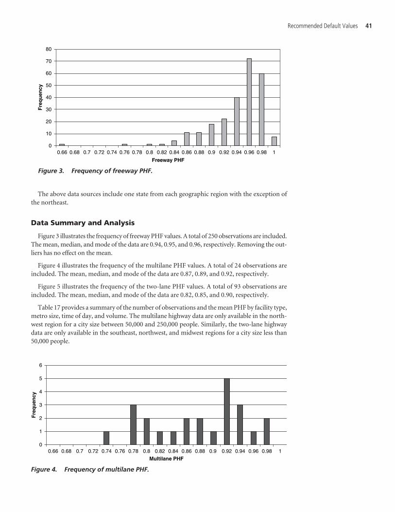
Recommended Default Values 41
0
10
20
30
40
50
60
70
80
0.66 0.68 0.7 0.72 0.74 0.76 0.78 0.8 0.82 0.84 0.86 0.88 0.9 0.92 0.94 0.96 0.98 1
Freeway PHF
Fre
qu
ency
Figure 3. Frequency of freeway PHF.
0
1
2
3
4
5
6
0.66 0.68 0.7 0.72 0.74 0.76 0.78 0.8 0.82 0.84 0.86 0.88 0.9 0.92 0.94 0.96 0.98 1
Multilane PHF
Fre
qu
ency
Figure 4. Frequency of multilane PHF.
The above data sources include one state from each geographic region with the exception ofthe northeast.
Data Summary and Analysis
Figure 3 illustrates the frequency of freeway PHF values. A total of 250 observations are included.The mean, median, and mode of the data are 0.94, 0.95, and 0.96, respectively. Removing the out-liers has no effect on the mean.
Figure 4 illustrates the frequency of the multilane PHF values. A total of 24 observations areincluded. The mean, median, and mode of the data are 0.87, 0.89, and 0.92, respectively.
Figure 5 illustrates the frequency of the two-lane PHF values. A total of 93 observations areincluded. The mean, median, and mode of the data are 0.82, 0.85, and 0.90, respectively.
Table 17 provides a summary of the number of observations and the mean PHF by facility type,metro size, time of day, and volume. The multilane highway data are only available in the north-west region for a city size between 50,000 and 250,000 people. Similarly, the two-lane highwaydata are only available in the southeast, northwest, and midwest regions for a city size less than50,000 people.

42 Default Values for Highway Capacity and Level of Service Analyses
0
2
4
6
8
10
12
14
16
0.58 0.6 0.62 0.64 0.66 0.68 0.7 0.72 0.74 0.76 0.78 0.8 0.82 0.84 0.86 0.88 0.9 0.92 0.94 0.96 0.98 1
Two-Lane PHF
Fre
qu
ency
Figure 5. Frequency of two-lane PHF.
Description Category FREEWAY MULTILANE TWO-LANE
#Obs Mean #Obs Mean #Obs Mean Southwest 77 0.93 0 NA 0 NA Southeast 28 0.94 0 NA 18 0.81
Northwest 18 0.93 24 0.87 12 0.84 Region
Midwest 126 0.94 0 NA 63 0.83
Northeast NA NA 0 NA 0 NA
>1.5M 39 0.94 0 NA 0 NA
250K-1.5M 147 0.94 0 NA 0 NA
50K-250K 60 0.93 24 0.87 0 NA City Size
<50K 3 0.90 0 NA 93 0.82
AM 91 0.92 8 0.84 32 0.81
MID 70 0.94 8 0.88 29 0.82 Period
PM 88 0.95 8 0.91 32 0.84
<500 19 0.89
501-1000 55 0.93
1001-1500 109 0.94
1501-2000 50 0.95
Hourly Volume /Lane
2001+ 16 0.95
<100 3 0.80 26 0.83
101-200 3 0.93 31 0.81
201-300 4 0.82 19 0.85
301-400 8 0.88 7 0.86
Hourly Volume/Lane
401+ 6 0.91 10 0.77
Table 17. PHF by region, metro size, and time of day.
Given the limited amount of multilane and two-lane data, it is difficult to draw conclusionsregarding mean PHF by region and city size. The freeway mean PHF is consistent across all regions.While the PHF appears to decrease with decreasing city size, there are few PHF observations forcities with less than 50,000 people.
In broad terms, the PHF is the highest for freeways, followed by multilane highways and thentwo-lane highways. There is a consistent trend in the data by time of day, with lower PHFs observedin the a.m. and higher PHFs observed in the p.m. There is also a consistent increase in the meanfreeway PHF as the volume per hour per lane increases. This trend is not observed for multilaneand two-lane highways, in part because of the lack of data. The type of facility and the time of dayare correlated to volume. That is, a freeway typically carries more vehicles per lane than a multi-lane or two-lane highway. Hence, the PHF is higher. Similarly, the observed volumes associatedwith the a.m. peak period are typically less than the volumes associated with the p.m. peak period.Thus, the PHF is smaller. Furthermore, the a.m. and p.m. peak periods have different types of trips
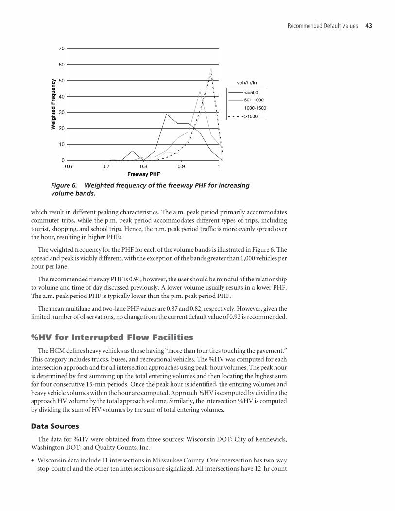
Recommended Default Values 43
0
10
20
30
40
50
60
70
0.6 0.7 0.8 0.9 1
Freeway PHF
Wei
gh
ted
Fre
qu
ency
<=500
501-1000
1000-1500
>1500
veh/hr/ln
Figure 6. Weighted frequency of the freeway PHF for increasing volume bands.
which result in different peaking characteristics. The a.m. peak period primarily accommodatescommuter trips, while the p.m. peak period accommodates different types of trips, includingtourist, shopping, and school trips. Hence, the p.m. peak period traffic is more evenly spread overthe hour, resulting in higher PHFs.
The weighted frequency for the PHF for each of the volume bands is illustrated in Figure 6. Thespread and peak is visibly different, with the exception of the bands greater than 1,000 vehicles perhour per lane.
The recommended freeway PHF is 0.94; however, the user should be mindful of the relationshipto volume and time of day discussed previously. A lower volume usually results in a lower PHF.The a.m. peak period PHF is typically lower than the p.m. peak period PHF.
The mean multilane and two-lane PHF values are 0.87 and 0.82, respectively. However, given thelimited number of observations, no change from the current default value of 0.92 is recommended.
%HV for Interrupted Flow Facilities
The HCM defines heavy vehicles as those having “more than four tires touching the pavement.”This category includes trucks, buses, and recreational vehicles. The %HV was computed for eachintersection approach and for all intersection approaches using peak-hour volumes. The peak houris determined by first summing up the total entering volumes and then locating the highest sumfor four consecutive 15-min periods. Once the peak hour is identified, the entering volumes andheavy vehicle volumes within the hour are computed. Approach %HV is computed by dividing theapproach HV volume by the total approach volume. Similarly, the intersection %HV is computedby dividing the sum of HV volumes by the sum of total entering volumes.
Data Sources
The data for %HV were obtained from three sources: Wisconsin DOT; City of Kennewick,Washington DOT; and Quality Counts, Inc.
• Wisconsin data include 11 intersections in Milwaukee County. One intersection has two-waystop-control and the other ten intersections are signalized. All intersections have 12-hr count

44 Default Values for Highway Capacity and Level of Service Analyses
0
50
100
150
200
250
300
350
0.0%
1.5%
3.0%
4.5%
6.0%
7.5%
9.0%
10.5
%
12.0
%
13.5
%
15.0
%
16.5
%
18.0
%
19.5
%
21.0
%
22.5
%
24.0
%
Intersection %HVF
req
uen
cy
Figure 7. Frequency of intersection %HV.
0
50
100
150
200
250
300
350
0 15 30 45 60 75 90
105
120
135
150
165
180
195
210
225
240
Intersection HV
Fre
qu
ency
Figure 8. Frequency of number of heavy vehicles.
data (6 a.m. to 6 p.m.) and include a state freeway or highway intersecting another state high-way or local street.
• Kennewick, Washington, data include over 100 intersections within the city limits. While themajority of the intersections are signalized, there are also about 10 two-way stop-controlledand 7 all-way stop-controlled intersections. Count data are available for 2 hr each during thea.m., p.m., and/or midday periods.
• The majority of the data was obtained from the Quality Counts (QC) database. These datainclude over 2,000 observations at signalized and unsignalized intersections in Arizona, Idaho,California, Florida, Maryland, Oregon, Utah, and Washington. Each observation representscounts conducted during the a.m., p.m., or midday period.
Data Summary and Analysis
Figure 7 illustrates the frequency of the intersection %HV for signalized, all-way stop-controlled,and two-way stop-controlled intersection types. A total of 2,314 observations are included. Sevenobservations have greater %HV than illustrated, with two observations at 100%. The %HV mean,median, and mode of the data is 3.6%, 2.5%, and 1.5%, respectively. Removing the outliers resultsin a mean of 3.4%.
Figure 8 illustrates the frequency of the number of heavy vehicles for signalized, all-way stop-controlled, and two-way stop-controlled intersection types. The mean, median, and mode of thedata are 52, 34, and 20 vehicles, respectively.

Table 18 provides a summary of the number of observations, mean %HV, and median %HV asa function of a number of discrete independent variables, including region, city size, intersectiontype, period (time of day), and approach volume.
Eighty-five percent of the data is represented in the northwest region. There are no obser-vations in the northeast and few observations in the midwest. Fifty-five percent of the data islocated in cities with greater than 1.5 million people. The %HV generally increases with adecrease in city size.
The data are well-represented for signalized intersections; however, little data are available forall-way stop-controlled intersections. Signalized intersection average %HV is lower than for thetwo-way stop-controlled and all-way stop-controlled intersections.
Approximately 50% of the %HV data was collected during the p.m. peak period. The peakperiod average %HV suggests that the time of day may have an influence on the mean %HV.That is, the a.m. peak period experiences a higher %HV than is experienced during other timesof the day.
The number of observations is well-represented in each volume category. The mean %HV tendsto decrease with decreasing total intersection volume. In most cases, the mean heavy vehicle per-centage falls within a range of 2.5% to 3.5%.
Recommended Default Values 45
Description Number of Observations
Mean%HV
Median%HV
REGION[1] Southwest 102 2.6% 1.7%[2] Southeast 226 4.0% 2.6%[3] Northwest 1949 3.6% 2.5% [4] Midwest 33 2.8% 2.5% [5] Northeast 0 NA NATOTAL 2310
CITY SIZE [1] >1.5M 1260 3.2% 2.1%[2] 250K to 1.5M 262 3.5% 2.8%[3] 50K to 250K 269 3.5% 2.8%[4] <50K 519 4.6% 3.3%TOTAL 2310
INTERSECTION TYPE [A] AWSC 81 3.6% 2.1%[S] SIGNALIZED 1645 3.4% 2.4%[T] TWSC 588 4.0% 2.7%TOTAL 2314
PERIOD[AM] 697 5.1% 4.4%[MID] 209 3.0% 1.4%[PM] 1279 2.8% 1.9%TOTAL 2185
TOTAL VEHICLES 500 385 4.1% 2.6%1000 473 3.7% 2.7%1500 428 3.6% 2.7%2000 316 3.4% 2.5%2500 243 3.2% 2.2%>2500 468 2.7% 2.1%TOTAL 2313
AWSC: all-way stop-controlledTWSC: two-way stop-controlled
Table 18. %HV by region, city, intersection control, peak period, and total intersection volume.
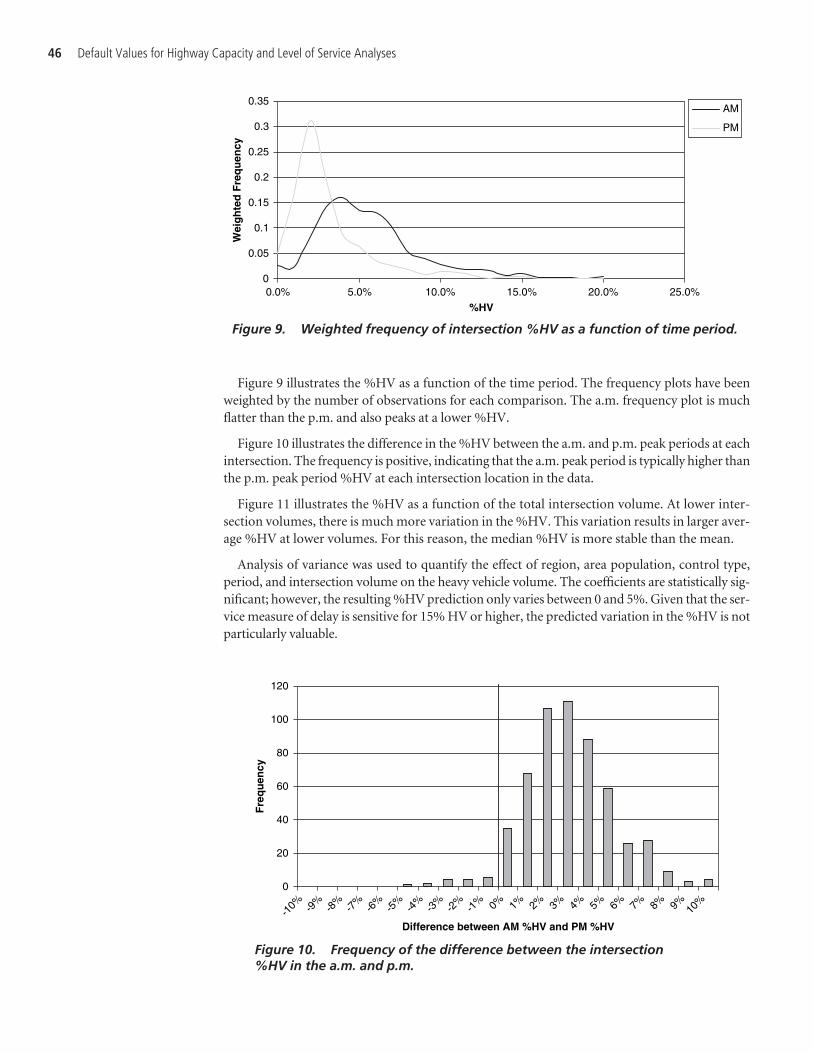
Figure 9 illustrates the %HV as a function of the time period. The frequency plots have beenweighted by the number of observations for each comparison. The a.m. frequency plot is muchflatter than the p.m. and also peaks at a lower %HV.
Figure 10 illustrates the difference in the %HV between the a.m. and p.m. peak periods at eachintersection. The frequency is positive, indicating that the a.m. peak period is typically higher thanthe p.m. peak period %HV at each intersection location in the data.
Figure 11 illustrates the %HV as a function of the total intersection volume. At lower inter-section volumes, there is much more variation in the %HV. This variation results in larger aver-age %HV at lower volumes. For this reason, the median %HV is more stable than the mean.
Analysis of variance was used to quantify the effect of region, area population, control type,period, and intersection volume on the heavy vehicle volume. The coefficients are statistically sig-nificant; however, the resulting %HV prediction only varies between 0 and 5%. Given that the ser-vice measure of delay is sensitive for 15% HV or higher, the predicted variation in the %HV is notparticularly valuable.
46 Default Values for Highway Capacity and Level of Service Analyses
0
0.05
0.1
0.15
0.2
0.25
0.3
0.35
0.0% 5.0% 10.0% 15.0% 20.0% 25.0%
%HV
Wei
gh
ted
Fre
qu
ency
AM
PM
Figure 9. Weighted frequency of intersection %HV as a function of time period.
0
20
40
60
80
100
120
-10% -9
%-8
%-7
%-6
%-5
%-4
%-3
%-2
%-1
% 0% 1% 2% 3% 4% 5% 6% 7% 8% 9% 10%
Difference between AM %HV and PM %HV
Fre
qu
ency
Figure 10. Frequency of the difference between the intersection %HV in the a.m. and p.m.

Recommended Default Values
The recommended %HV is 3%, which is slightly higher than the current HCM default of 2%.The user should be aware of the relationship with volume, period, and city size, as indicated in theanalysis above. As volume decreases, the %HV tends to increase. The %HV is typically lower dur-ing the a.m. peak period than during the p.m. peak period, and the %HV increases with decreas-ing city size.
PHFs for Interrupted Flow Facilities
The HCM defines PHF as “a measure of traffic demand fluctuation within the peak hour.” Thiscan be computed by dividing the peak hourly volume by the peak 15-min flow rate within that peakhour. Because the existing definition in the HCM is general in nature, there are a number of dif-ferent methods available to calculate PHFs at an intersection. Three popular methods are describedas follows:
• Use the total entering volume to determine the peak 15-min interval and the peak hour. Sub-sequently, compute an overall intersection PHF. This approach yields the correct total volumeduring the peak 15-min time period, but may underestimate or overestimate the demands forthe individual approaches and/or movements.
• Use the total approach volume to determine the peak 15-min interval and the peak hour.Subsequently, compute individual approach PHFs. Thus, a four-leg intersection wouldhave four PHFs and a T-junction would have three PHFs. This approach, while used inpractice (and perhaps encouraged by the HCM methodology), is fundamentally flawed in that it assumes that the individual approaches peak during the same time period, whichrarely occurs. The result is a high likelihood of overestimating the total volume during thepeak 15-min time period.
• Use the movement volume to determine the peak 15-min interval and the peak hour. Subse-quently, compute individual movement PHFs. Thus, a four-leg intersection with left-through-right movements would have 12 PHFs. This approach is also fundamentally flawed in that itassumes that the individual movements peak during the same time period, which is extremelyrare. The result is a very high likelihood of overestimating the total volume during the peak15-min time period.
There are other variations of these methods. The total intersection volume method (the firstmethod described above) is the only method that yields the correct total intersection flow rate.Calculating the approach or movement PHF assumes that each of the approaches or individualmovements peak during the same time period, which is unlikely to occur.
Recommended Default Values 47
0.0%
5.0%
10.0%
15.0%
20.0%
0 1,000 2,000 3,000 4,000 5,000
Total Intersection Volume
%H
V
Figure 11. %HV as a function of total intersection volume.

Data Sources
Seven sources of useable PHF data were obtained. The seven sources are the Delaware DOT;Wisconsin DOT, the City of Kennewick, Washington; the City of Los Angeles; VRPA Technolo-gies, Inc.; Tucson, Arizona; and Quality Counts, Inc. All data for PHF estimation were based onactual traffic counts collected in 15-min intervals—mostly in 2005 and 2006. Further, most dataare typical weekday counts (i.e., Tuesday, Wednesday, or Thursday) that were conducted duringone or more of the peak periods.
• Delaware DOT and Wisconsin DOT data were provided in MS Excel and PDF formats andincluded a number of intersections in various counties. All intersections have 12-hr count data(6 a.m. to 6 p.m.) in 15-min intervals and comprise of a state highway intersecting another statehighway or local street.
• The City of Kennewick, Washington, provided data in PDF format for over 100 intersectionswithin the city limits. While the majority of the intersections were signalized intersections, therewere also ten two-way stop-controlled and seven all-way stop-controlled intersections. Countdata were available for 2 hr each for the a.m., p.m., and/or midday periods in 15-min intervals.
• The largest data set was provided by the Quality Counts (QC) database. The data were providedin both PDF and MS Excel formats. The data comprised over 2,000 intersection counts at sig-nalized and unsignalized intersections in Arizona, Idaho, California, Florida, Maryland, Ore-gon, Utah, and Washington. Each observation represented counts conducted during the a.m.,p.m., or midday periods. The counts are typically in 5-min or 15-min intervals.
• The Pima Association of Governments (PAG) in Tucson, Arizona, provided data in MS Excelformat at 16 major signalized intersections. All data were collected in spring 2006. Each inter-section data set included 2 hr of 15-min counts for the a.m., midday, and p.m. peak periods.
• VRPA Technologies, Inc., provided data at eight intersections in Fresno, California; 10 inter-sections in Riverside, California; and 15 intersections in San Diego, California. The data wereprovided in MS Excel format and included both a.m. and p.m. peak counts in 15-min intervals.
Data Summary and Analysis
Figure 12 illustrates the frequency of the intersection PHF for signalized, two-way stop-controlled and all-way stop-controlled intersection types. The PHF mean, median, and mode ofthe data were found to be 0.89, 0.93, and 0.93 to 0.94, respectively. Removing the few outliers withPHF values of less than 0.70 resulted in a mean PHF of 0.90.
For planning purposes, the PHF for the major street volume was also calculated. As shown inFigure 13, the intersection PHF and major street PHF are heavily correlated. This could be helpful
48 Default Values for Highway Capacity and Level of Service Analyses
Figure 12. Frequency of intersection PHF.
0
50
100
150
200
250
0.34 0.39 0.44 0.49 0.54 0.59 0.64 0.69 0.74 0.79 0.84 0.89 0.94 0.99
PHF
Fre
qu
ency

in situations where the user only had PHF data for the major street (based on tube count data forexample).
Table 19 provides a summary of the number of observations, mean intersection PHF, andmedian PHF as a function of a number of discrete independent variables, including region, citysize, intersection control, peak period (time of day) and volume. As indicated in the table, 78% ofthe data is represented in the northwest region. There are few observations in the northeast andmidwest. Fifty-four percent of the data is located in cities with greater than 1.5 million people.Approximately 60% of the PHF data occurs in the p.m. peak period.
As indicated in Table 19, with the exception of the total intersection volume and time of day,most of the variables do not indicate any trend in the mean or median.
Figure 14 illustrates the intersection PHF as a function of total intersection volume. At lowertotal volumes, there is more variation in the PHF. This variation results in larger mean PHF atlower volumes. The median also indicates a similar trend. The median was found to be 0.93. Basedon the results of the analysis, the current HCM default value of 0.92 appears to be reasonable whenthe total entering volume is greater than 1,000 vehicles. A more-conservative PHF (below 0.90) islikely to occur when the total entering volume is less than 1,000 vehicles.
Figure 15 illustrates the weighted frequency of the PHF for the a.m. and p.m. peak periods. Thea.m. peak period has a greater spread and a lower peak PHF than the p.m. peak period. The a.m.and p.m. peak periods have different types of trips which result in different peaking characteristics.The a.m. peak period primarily consists of commuter trips, while the p.m. peak period containsdifferent types of trips including tourist, shopping, and school trips. Hence, the p.m. peak periodtraffic is more evenly spread over the hour, resulting in higher PHF.
Recommended Default Values
Intersection PHF (rather than approach or movement PHF) has been used to determine the rec-ommended PHF default value. The total intersection volume method is the only method that yieldsthe correct total intersection volume. Approach or movement PHF assumes each of the approachesor individual movements peak during the same time period, which is unlikely to occur.
Based on the results of this analysis, the current HCM default value of 0.92 appears to be rea-sonable. The user should be aware of the relationship of PHF with volume and time of day. A
Recommended Default Values 49
Figure 13. Intersection PHF as a function of majorstreet PHF.
y = 0.9301x + 0.0549R2 = 0.836
0.4
0.6
0.8
1
0.4 0.6 0.8 1
Major Street PHF
To
tal I
nte
rsec
tio
n P
HF
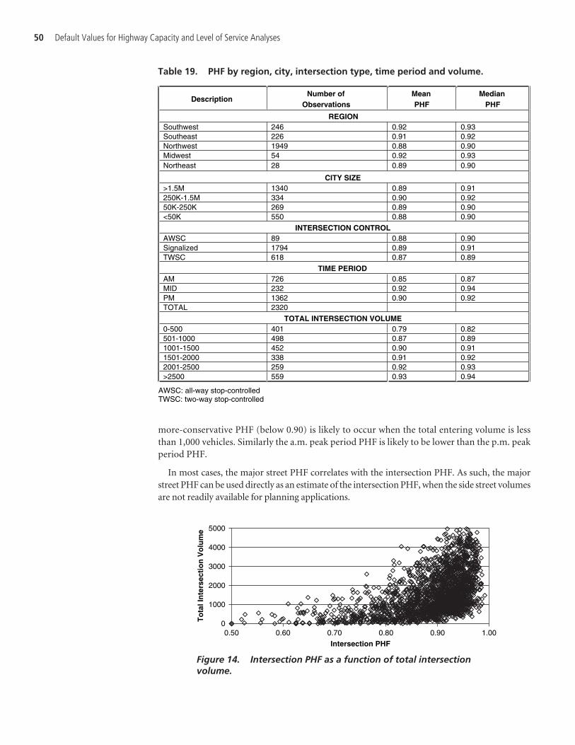
50 Default Values for Highway Capacity and Level of Service Analyses
Table 19. PHF by region, city, intersection type, time period and volume.
Description Number of
ObservationsMeanPHF
MedianPHF
REGION Southwest 246 0.92 0.93 Southeast 226 0.91 0.92 Northwest 1949 0.88 0.90 Midwest 54 0.92 0.93 Northeast 28 0.89 0.90
CITY SIZE >1.5M 1340 0.89 0.91 250K-1.5M 334 0.90 0.92 50K-250K 269 0.89 0.90 <50K 550 0.88 0.90
INTERSECTION CONTROL AWSC 89 0.88 0.90 Signalized 1794 0.89 0.91 TWSC 618 0.87 0.89
TIME PERIOD AM 726 0.85 0.87 MID 232 0.92 0.94 PM 1362 0.90 0.92 TOTAL 2320
TOTAL INTERSECTION VOLUME 0-500 401 0.79 0.82 501-1000 498 0.87 0.89 1001-1500 452 0.90 0.91 1501-2000 338 0.91 0.92 2001-2500 259 0.92 0.93 >2500 559 0.93 0.94
AWSC: all-way stop-controlled TWSC: two-way stop-controlled
Figure 14. Intersection PHF as a function of total intersectionvolume.
0
1000
2000
3000
4000
5000
0.50 0.60 0.70 0.80 0.90 1.00
Intersection PHF
To
tal I
nte
rsec
tio
n V
olu
me
more-conservative PHF (below 0.90) is likely to occur when the total entering volume is lessthan 1,000 vehicles. Similarly the a.m. peak period PHF is likely to be lower than the p.m. peakperiod PHF.
In most cases, the major street PHF correlates with the intersection PHF. As such, the majorstreet PHF can be used directly as an estimate of the intersection PHF, when the side street volumesare not readily available for planning applications.
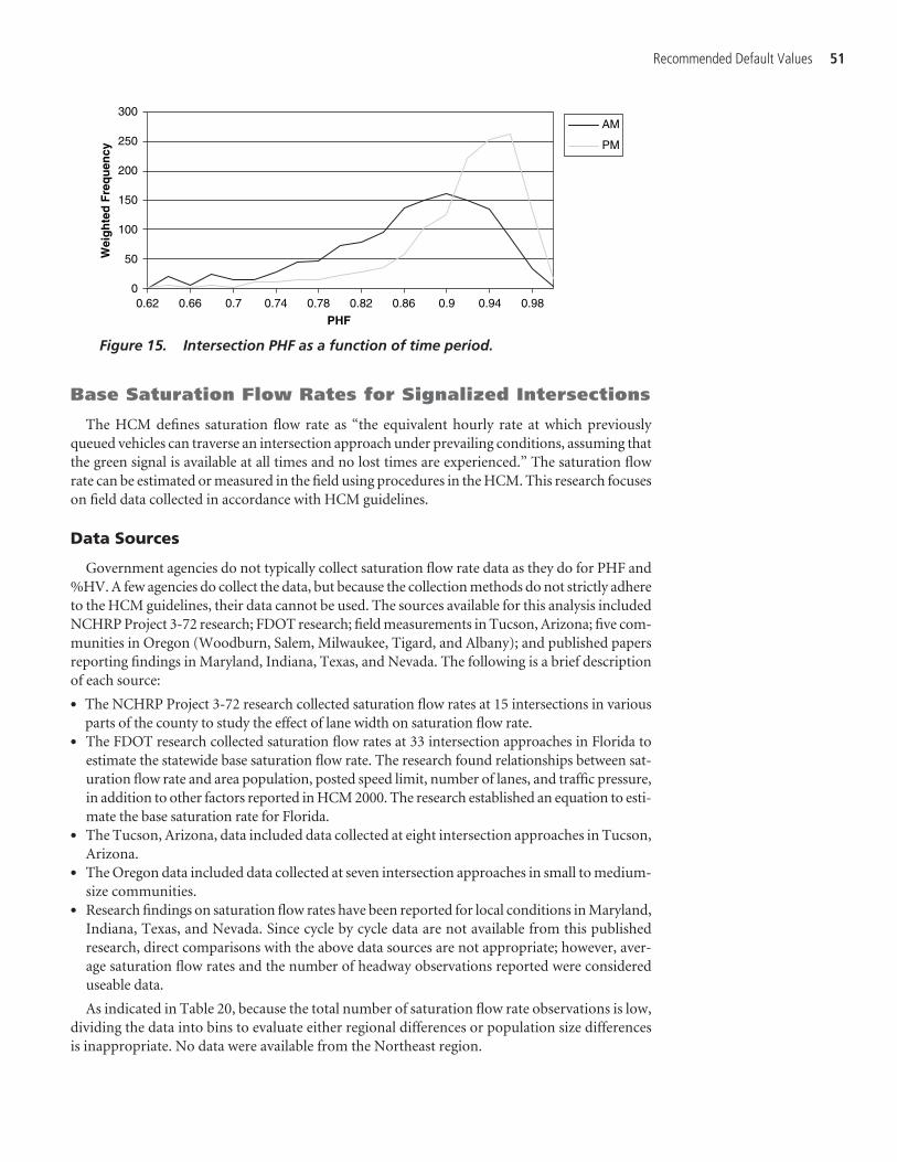
Base Saturation Flow Rates for Signalized Intersections
The HCM defines saturation flow rate as “the equivalent hourly rate at which previouslyqueued vehicles can traverse an intersection approach under prevailing conditions, assuming thatthe green signal is available at all times and no lost times are experienced.” The saturation flowrate can be estimated or measured in the field using procedures in the HCM. This research focuseson field data collected in accordance with HCM guidelines.
Data Sources
Government agencies do not typically collect saturation flow rate data as they do for PHF and%HV. A few agencies do collect the data, but because the collection methods do not strictly adhereto the HCM guidelines, their data cannot be used. The sources available for this analysis includedNCHRP Project 3-72 research; FDOT research; field measurements in Tucson, Arizona; five com-munities in Oregon (Woodburn, Salem, Milwaukee, Tigard, and Albany); and published papersreporting findings in Maryland, Indiana, Texas, and Nevada. The following is a brief descriptionof each source:
• The NCHRP Project 3-72 research collected saturation flow rates at 15 intersections in variousparts of the county to study the effect of lane width on saturation flow rate.
• The FDOT research collected saturation flow rates at 33 intersection approaches in Florida toestimate the statewide base saturation flow rate. The research found relationships between sat-uration flow rate and area population, posted speed limit, number of lanes, and traffic pressure,in addition to other factors reported in HCM 2000. The research established an equation to esti-mate the base saturation rate for Florida.
• The Tucson, Arizona, data included data collected at eight intersection approaches in Tucson,Arizona.
• The Oregon data included data collected at seven intersection approaches in small to medium-size communities.
• Research findings on saturation flow rates have been reported for local conditions in Maryland,Indiana, Texas, and Nevada. Since cycle by cycle data are not available from this publishedresearch, direct comparisons with the above data sources are not appropriate; however, aver-age saturation flow rates and the number of headway observations reported were considereduseable data.
As indicated in Table 20, because the total number of saturation flow rate observations is low,dividing the data into bins to evaluate either regional differences or population size differencesis inappropriate. No data were available from the Northeast region.
Recommended Default Values 51
Figure 15. Intersection PHF as a function of time period.
0
50
100
150
200
250
300
0.62 0.66 0.7 0.74 0.78 0.82 0.86 0.9 0.94 0.98
PHF
Wei
gh
ted
Fre
qu
ency
AM
PM
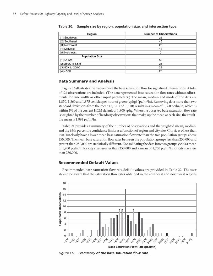
Data Summary and Analysis
Figure 16 illustrates the frequency of the base saturation flow for signalized intersections. A totalof 124 observations are included. (The data represented base saturation flow rates without adjust-ments for lane width or other input parameters.) The mean, median and mode of the data are1,850, 1,860 and 1,875 vehicles per hour of green (vphg) (pc/hr/ln). Removing data more than twostandard deviations from the mean (2,190 and 1,510) results in a mean of 1,860 pc/hr/ln, which iswithin 2% of the current HCM default of 1,900 vphg. When the observed base saturation flow rateis weighted by the number of headway observations that make up the mean at each site, the result-ing mean is 1,894 pc/hr/ln.
Table 21 provides a summary of the number of observations and the weighted mean, median,and the 95th percentile confidence limits as a function of region and city size. City sizes of less than250,000 clearly have a lower mean base saturation flow rate than the two population groups above250,000. The mean base saturation flow rates between the population groups less than 250,000 andgreater than 250,000 are statistically different. Consolidating the data into two groups yields a meanof 1,900 pc/hr/ln for city sizes greater than 250,000 and a mean of 1,750 pc/hr/ln for city sizes lessthan 250,000.
Recommended Default Values
Recommended base saturation flow rate default values are provided in Table 22. The usershould be aware that the saturation flow rates obtained in the southeast and northwest regions
52 Default Values for Highway Capacity and Level of Service Analyses
Table 20. Sample size by region, population size, and intersection type.
Region Number of Observations[1] Southwest 23[2] Southeast 43[3] Northwest 25[4] Midwest 43[5] Northeast 0
Population Size[1] >1.5M 58[2] 250K to 1.5M 25[3] 50K to 250K 28[4] <50K 23
Figure 16. Frequency of the base saturation flow rate.
0
2
4
6
8
10
12
14
16
18
1375
1425
1475
1525
1575
1625
1675
1725
1775
1825
1875
1925
1975
2025
2075
2125
2175
2225
2275
2325
2375
2425
2475
Base Saturation Flow Rate (pc/hr/ln)
# A
pp
roac
h O
bse
rvat
ion
s
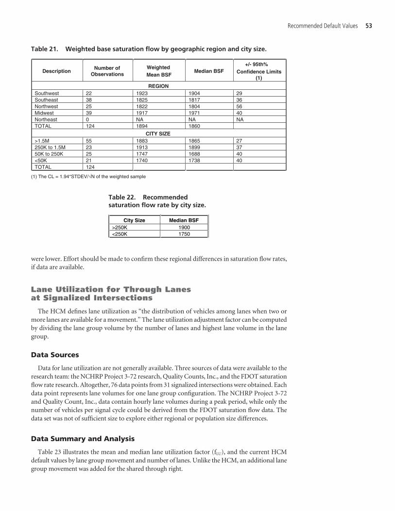
were lower. Effort should be made to confirm these regional differences in saturation flow rates,if data are available.
Lane Utilization for Through Lanes at Signalized Intersections
The HCM defines lane utilization as “the distribution of vehicles among lanes when two ormore lanes are available for a movement.” The lane utilization adjustment factor can be computedby dividing the lane group volume by the number of lanes and highest lane volume in the lanegroup.
Data Sources
Data for lane utilization are not generally available. Three sources of data were available to theresearch team: the NCHRP Project 3-72 research, Quality Counts, Inc., and the FDOT saturationflow rate research. Altogether, 76 data points from 31 signalized intersections were obtained. Eachdata point represents lane volumes for one lane group configuration. The NCHRP Project 3-72and Quality Count, Inc., data contain hourly lane volumes during a peak period, while only thenumber of vehicles per signal cycle could be derived from the FDOT saturation flow data. Thedata set was not of sufficient size to explore either regional or population size differences.
Data Summary and Analysis
Table 23 illustrates the mean and median lane utilization factor (fLU), and the current HCMdefault values by lane group movement and number of lanes. Unlike the HCM, an additional lanegroup movement was added for the shared through right.
Recommended Default Values 53
Table 21. Weighted base saturation flow by geographic region and city size.
Description Number of
ObservationsWeightedMean BSF
Median BSF +/- 95th%
Confidence Limits (1)
REGION Southwest 22 1923 1904 29 Southeast 38 1825 1817 36 Northwest 25 1822 1804 56 Midwest 39 1917 1971 40 Northeast 0 NA NA NA TOTAL 124 1894 1860
CITY SIZE >1.5M 55 1883 1865 27 250K to 1.5M 23 1913 1899 37 50K to 250K 25 1747 1688 40 <50K 21 1740 1738 40 TOTAL 124
(1) The CL = 1.94*STDEV/ N of the weighted sample
Table 22. Recommended saturation flow rate by city size.
City Size Median BSF >250K 1900<250K 1750
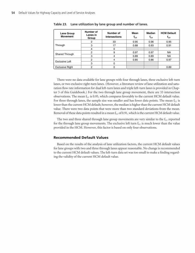
There were no data available for lane groups with four through lanes, three exclusive left-turnlanes, or two exclusive right-turn lanes. (However, a literature review of lane utilization and satu-ration flow rate information for dual left-turn lanes and triple left-turn lanes is provided in Chap-ter 5 of this Guidebook.) For the two through lane group movement, there are 33 intersectionobservations. The mean fLU is 0.95, which compares favorably to the current HCM default value.For three through lanes, the sample size was smaller and has fewer data points. The mean fLU islower than the current HCM default; however, the median is higher than the current HCM defaultvalue. There were two data points that were more than two standard deviations from the mean.Removal of these data points resulted in a mean fLU of 0.91, which is the current HCM default value.
The two and three shared through lane group movements are very similar to the fLU reportedfor the through lane group movements. The exclusive left turn fLU is much lower than the valueprovided in the HCM. However, this factor is based on only four observations.
Recommended Default Values
Based on the results of the analysis of lane utilization factors, the current HCM default valuesfor lane groups with two and three through lanes appear reasonable. No change is recommendedto the current HCM default values. The left-turn data set was too small to make a finding regard-ing the validity of the current HCM default value.
54 Default Values for Highway Capacity and Level of Service Analyses
Table 23. Lane utilization by lane group and number of lanes.
Lane Group Movement
Number ofLanes inGroup
Number ofIntersections
MeanfLU
MedianfLU
HCM Default fLU
2 33 0.95 0.96 0.95 3 17 0.88 0.93 0.91 Through
4 0 2 9 0.97 0.97 NA
Shared Through 3 4 0.89 0.89 NA 2 4 0.85 0.86 0.97
Exclusive Left 3 0
Exclusive Right 2 0 0.89

This chapter provides information for input parameters where field data were not available.Default value guidance was developed based on a review of relevant research literature. Thisguidance is provided for six input parameters:
• Pedestrian walking speeds and start-up times at signalized intersections• Lane utilization, traffic pressure, and distance between intersections for interchange ramp
terminals• Driver population factors on freeways• Signal density on urban streets• Free-flow speed on urban streets• Saturation flow rates and lane utilization factors for dual and triple left-turn lanes at signalized
intersections
Pedestrian Walking Speeds and Start-up Times at Signalized Intersections
Pedestrian walking speeds and start-up times are used in the analyses of signalized intersections,unsignalized (two-way stop-controlled) intersections, and pedestrian facilities—including walk-ways, shared off-street paths, crosswalks (signalized and unsignalized), and sidewalks along urbanstreets. There are a range of pedestrian walking speed values in the HCM, depending on the facil-ity type to be analyzed. These walking speed values are described in Table 24. In general, a defaultpedestrian walking speed of 4 ft/s is provided, with the exception of the exclusive shared pedestrianand bicycle facilities, which assume a much faster walking speed of 5.0 ft/s. For exclusive pedestrianfacilities where a mix of more than 20% elderly population is present, a default value of 3.3 ft/s isprovided.
The source of the 4.0 ft/s default value for pedestrian walking speed is the Manual on UniformTraffic Control Devices (MUTCD). This walking speed represents the 15th percentile pedestrianpopulation. Therefore, it is intended to accommodate pedestrians who walk at speeds slower thanthe average. Pedestrian start-up times are used in the calculation of delay at a signalized intersectionto determine the minimum pedestrian green time at crosswalks. The current HCM default valuefor pedestrian start-up time at an intersection is 3.2 s. Uninterrupted flow pedestrian facility servicemeasures are highly sensitive to pedestrian walking speed. In addition, pedestrian walking speed isused extensively in the analysis of intersections. For these reasons, pedestrian walking speeds war-rant further guidance.
Summary of Relevant Research
Several national publications were reviewed with respect to pedestrian walking speeds. A sum-mary of the policy guidance from various sources on pedestrian walking speeds is provided in
55
C H A P T E R 4
Guidance for Selecting Defaults

Table 25. In the next edition of the MUTCD, a walking speed of 3.5 ft/s will be assumed for a sig-nalized crosswalk when calculating the Flashing Don’t Walk from the near side curb or shoulderto the far side of the traveled way or median of sufficient width for pedestrians to wait. The guid-ance will also include a separate calculation for the total pedestrian time (Walk plus Flashing Don’tWalk) using a default walking speed of 3.0 ft/s from 6 ft behind the curb to the far side of the trav-eled way. (The distance of 6 ft behind the near side curb is assumed to represent the curb ramplength.) The Walk interval is calculated as the difference between the total pedestrian time and theFlashing Don’t Walk interval. A minimum walk interval of 4 s still applies in this new procedure.The calculated times represent minimums needed to satisfy the assumed walking speed and cross-ing distance at a signalized crosswalk. The additional time that is required to satisfy pedestriandemand should be added to the pedestrian walk interval.
Table 26 provides examples of the total pedestrian time and the walk interval for various streetwidths plus an assumed ramp length of 6 ft. This pedestrian crossing time is based on the MUTCDadopted 3.0 ft/s walking speed used in total pedestrian time calculation and 3.5 ft/s speeds usedin the Flashing Don’t Walk calculation.
Table 27 summarizes recent pedestrian speed studies. As indicated, the pedestrian walkingspeeds vary between 2.8 ft/s and 4.0 ft/s. Elderly walking speed observations range from 2.8 to3.5 ft/s. Although there is no universal value for pedestrian walking speeds, it is clear that the cur-rent HCM default value of 4.0 ft/s does not sufficiently accommodate elderly pedestrians.
56 Default Values for Highway Capacity and Level of Service Analyses
FacilityType
SubFacility
LOSMeasure
ParameterImpactingLOS ThatUses Ped
Speed
Comment HCM2000
DefaultValue
Ped Signal Vehicle Delay(s/veh)
Ped AdjustmentFactor
Uses derivative of ped speed for Walk & Flash Don’t Walk (FDW)Walk—4–7 (s)FDW—4–7 (s)
NASignalizedIntersections
No Ped Signal
Vehicle Delay(s/veh)
Min Ped Green Time
Not directly used in the delay equation, but rather to ensure minimum green splits are met
4 ft/s
TWSC Intersections Vehicle Delay (s/veh)
Ped Blockage Factor
4 ft/s
AWSC Intersections and Roundabouts:
Vehicle Delay (s/veh)
NA Ped speed is not used NA
SignalTime-space (ft2/s)
Time-space 4 ft/s
UnsignalizedPed Delay (s/ped)
Critical Ped Gap Example Problem uses 3 ft/s 4 ft/s InterruptedPed Facilities
StreetsAve Ped Speed (ft/s)
Ave Ped Speed Uninterrupted or interrupted; combines street segments and intersections
4 ft/s
Uninterrupted Exclusive Ped Facilities
Ave Ped Flow (ped/hr)
Ave Ped Flow
4 ft/s for a ped mix with up to20% elderly (65 years+)3.3 ft/s for a ped mix with anexcess of 20% elderly
4 ft/s;3.3 ft/s
Uninterrupted Shared Ped and Bike Facilities
# of Passing & Opposing Events
# of Passing & OpposingEvents
Assumes an 8.0-ft wide path 5 ft/s
AWSC: all-way stop-controlled TWSC: two-way stop-controlled
Table 24. Summary of HCM 2000 pedestrian speed default parameters.
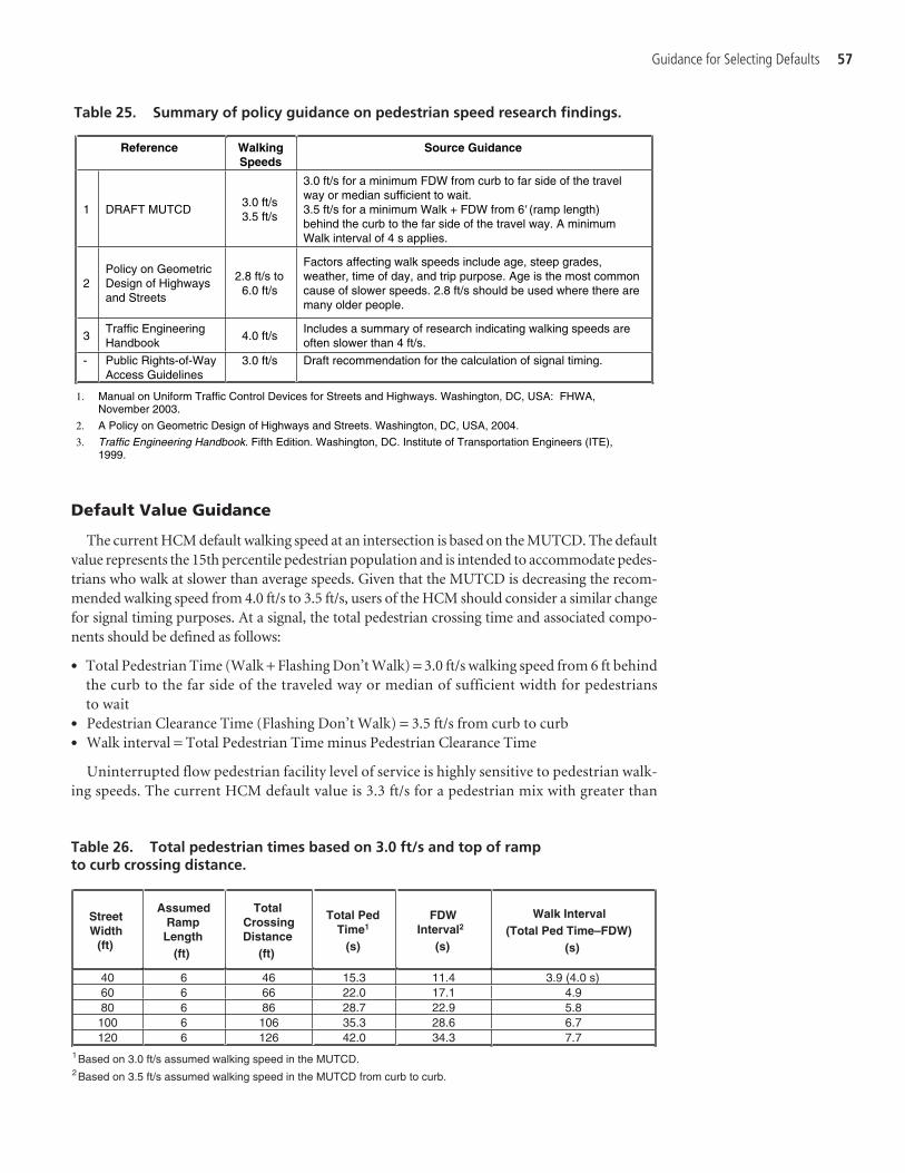
Default Value Guidance
The current HCM default walking speed at an intersection is based on the MUTCD. The defaultvalue represents the 15th percentile pedestrian population and is intended to accommodate pedes-trians who walk at slower than average speeds. Given that the MUTCD is decreasing the recom-mended walking speed from 4.0 ft/s to 3.5 ft/s, users of the HCM should consider a similar changefor signal timing purposes. At a signal, the total pedestrian crossing time and associated compo-nents should be defined as follows:
• Total Pedestrian Time (Walk + Flashing Don’t Walk) = 3.0 ft/s walking speed from 6 ft behindthe curb to the far side of the traveled way or median of sufficient width for pedestrians to wait
• Pedestrian Clearance Time (Flashing Don’t Walk) = 3.5 ft/s from curb to curb• Walk interval = Total Pedestrian Time minus Pedestrian Clearance Time
Uninterrupted flow pedestrian facility level of service is highly sensitive to pedestrian walk-ing speeds. The current HCM default value is 3.3 ft/s for a pedestrian mix with greater than
Guidance for Selecting Defaults 57
Reference WalkingSpeeds
Source Guidance
1 DRAFT MUTCD 3.0 ft/s 3.5 ft/s
3.0 ft/s for a minimum FDW from curb to far side of the travel way or median sufficient to wait.3.5 ft/s for a minimum Walk + FDW from 6' (ramp length)behind the curb to the far side of the travel way. A minimum Walk interval of 4 s applies.
2Policy on Geometric Design of Highwaysand Streets
2.8 ft/s to 6.0 ft/s
Factors affecting walk speeds include age, steep grades, weather, time of day, and trip purpose. Age is the most commoncause of slower speeds. 2.8 ft/s should be used where there are many older people.
3Traffic Engineering Handbook
4.0 ft/s Includes a summary of research indicating walking speeds are often slower than 4 ft/s.
- Public Rights-of-Way Access Guidelines
3.0 ft/s Draft recommendation for the calculation of signal timing.
1. Manual on Uniform Traffic Control Devices for Streets and Highways. Washington, DC, USA: FHWA, November 2003.
2. A Policy on Geometric Design of Highways and Streets. Washington, DC, USA, 2004.
3. Traffic Engineering Handbook. Fifth Edition. Washington, DC. Institute of Transportation Engineers (ITE),1999.
Table 25. Summary of policy guidance on pedestrian speed research findings.
StreetWidth
(ft)
AssumedRamp
Length(ft)
TotalCrossingDistance
(ft)
Total Ped Time1
(s)
FDWInterval2
(s)
Walk Interval(Total Ped Time–FDW)
(s)
40 6 46 15.3 11.4 3.9 (4.0 s) 60 6 66 22.0 17.1 4.9 80 6 86 28.7 22.9 5.8 100 6 106 35.3 28.6 6.7 120 6 126 42.0 34.3 7.7
1 Based on 3.0 ft/s assumed walking speed in the MUTCD. 2 Based on 3.5 ft/s assumed walking speed in the MUTCD from curb to curb.
Table 26. Total pedestrian times based on 3.0 ft/s and top of ramp to curb crossing distance.

20% elderly. Given the range of speeds collected for elderly pedestrians (between 2.8 and 3.5 ft/s), the use of 3.3 ft/s is a reasonable value where there is limited data regarding the proportion of elderly pedestrians. For shared uninterrupted pedestrian-bicycle facilities, theHCM default value is 5.0 ft/s. Because the literature does not specifically examine these typesof facilities, care should be taken in the consideration of the user’s age, the facility grades, andtrip purpose.
Interchange Ramp Terminals
A new version of Chapter 26 of the HCM (Interchange Ramp Terminals) has been approved bythe Committee on Highway Capacity and Quality of Service. A methodology for conducting bothoperations and planning analyses for at-grade intersections (interchange ramp terminals) in thevicinity of freeway interchanges is now provided. This new chapter addresses diamond inter-changes, PARCLOs, and single-point urban interchanges. The operations assessment relies on spe-cific traffic and interchange information. The level of service is then calculated for each of the move-ments at the interchange, based on the total average control delay. The analysis of interchange rampterminals requires the adjustment of a base saturation flow rate similar to the adjustment thatoccurs for signalized intersections. At interchange ramp terminals, different adjustments for traf-fic pressure and lane utilization at the external arterial approaches are determined. In addition,most interchange ramp terminal analyses involve the presence of two closely spaced intersections.The distance separating these two intersections is also a critical consideration in the operationalanalysis. Since the remaining input parameters for interchange ramp terminals are similar to theinput parameter for an individual signalized intersection, the specific input parameters of interestfor interchange ramp terminals include
• Lane utilization (external approaches only),• Traffic pressure, and• Distance between intersections within interchange.
58 Default Values for Highway Capacity and Level of Service Analyses
Reference Walking Speeds
Source Guidance
1 Fitzpatrick et al. 3.8 ft/s 3.5 ft/s
Year 2005 data from 42 sites in seven states;3.8 ft/s 15th percentile walking speeds <60 years of age3.5 ft/s 15th percentile walking speeds > 60 years of age or less able
2 Gates et al. 2.9 ft/s to
3.8 ft/s
Year 2005 data from 11 sites 2.9 ft/s for locations with 100% peds > 65 years of age 3.6, 3.5, 3.4, 3.3 ft/s for 20, 30, 40, and 50% mix of peds > 65 years of age
3 Knoblauch et al.4.0 ft/s 3.1 ft/s
4.0 ft/s 15th percentile speeds for peds< 65 years of age3.1 ft/s 15th percentile speeds for peds > 65 years of age
4 Staplin et al. 2.8 ft/s Older pedestrians
1. Fitzpatrick, K., Brewer, M.A., and Turner, S. Another Look at Pedestrian Walking Speed. 85th Annual Meeting of the Transportation Research Board, CD-ROM. November 2005.
2. Gates, T.J., Noyce, D.A., Bill A.R., and Van Ee, N. Recommended Walking Speeds for Pedestrian Clearance Timing Based on Pedestrian Characteristics. 85th Annual Meeting of the Transportation Research Board, CD-ROM. November 2005.
3. Knoblauch, R.L., Pietrucha, M.T., and Nitzburg, M. Field Studies of Pedestrian Walking Speed and Start-Up Time. Transportation Research Record No. 1538 (1996): 27-38.
4. Staplin, L., Lococo, K., Byington, S., and Harkey, D. Guidelines and Recommendations to Accommodate Older Drivers and Pedestrians. FHWA. Publication No. FHWA-RD-01-051. May 2001.
Table 27. Summary of pedestrian speed studies.

Lane Utilization
At interchange ramp terminals, the lane utilization adjustment factors are calculated in the samemanner as at an individual signalized intersection with the exception of the external arterialapproaches. On the external arterial approaches, vehicles do not distribute as evenly among lanesin a lane group as at signalized intersections. Factors contributing to the unequal traffic distribu-tion at the external arterial approaches include high turning movements at the downstream inter-section and short internal link distances within the interchange. An example of this is the high vol-ume of vehicles moving into the left lanes at an upstream intersection of an interchange to preparefor a left turn at the downstream intersection.
To account for this, models were developed to estimate percent of total flow in the externalarterial approach lanes. The input data required for these models include:
• Interchange type• Number of external arterial approach lanes (2, 3, or 4 lanes), and• Origin-destination (O-D) demands from the external arterial approaches through the inter-
change (veh/hr).
To simplify calculation of the lane utilization factor of an external arterial approach to a partic-ular interchange type, lookup tables were developed during the research project that led to the newInterchange Ramp Terminal chapter. These tables include several origin-destination movementdistributions for each interchange type’s exterior arterial approaches and the resulting lane uti-lization adjustment factors for 2-lane, 3-lane, and 4-lane approaches. (The only configuration notincluded in these tables is for the case of the diamond interchange with 2-lane arterial approaches.The lane utilization factor for this configuration requires the distance between intersections withinthe interchange.) These lookup tables have been simplified to facilitate their use. These simplifiedtables are provided in Appendix B of this Guidebook.
Traffic Pressure Adjustment Factor
Traffic pressure is used to adjust the ideal saturation flow rate in interchange ramp terminalanalyses. This input parameter reflects the display of aggressive driving behavior by a large num-ber of drivers during high-demand traffic conditions when shorter than usual headways areaccepted during queue discharge. The traffic pressure for various demand flow rates and move-ment types are illustrated in Table 28 and Table 29. The demand flow rates are expressed in vehi-cles per cycle per hour (vpcph). Interchange turning movement counts are more typicallyexpressed as vehicles per hour per movement. Therefore, these tables were developed to relateapproach counts (vph) and demand flow rates by movement type and several cycle lengths(80 s, 100 s, 120 s, 140 s, and 160 s). The demand flow rates include a minimum of 1 vpcph to amaximum of 30 vpcph. The effects of demand flow rates greater than 30 vpcph are not knownand the use of 30 vpcph should be used when analyzing higher flow rates.
As shown in these tables, demand flow rates of 14 vpcph or less result in traffic pressure adjust-ment factors less than 1.0 for through or right-turn movements. For left-turn movements, demandflow rates of 10 vpcph or less result in traffic pressure adjustment factors less than 1.0. Thus, it canbe concluded that demand flow rates at or below these levels reduce the saturation flow rate whilegreater levels (i.e., shorter headways) increase the saturation flow rate.
Distance between Two Intersections within an Interchange
One of the primary geometric input parameters in the analysis of interchange ramp terminalsis the distance between intersections within the interchange. This information is typically easy to
Guidance for Selecting Defaults 59

obtain for existing interchanges from sources such as field measurements, as-built drawings, orscaled aerial photos. For analysis of future interchange conditions, the distance between inter-sections can be estimated from conceptual plans or from construction documents. For operationaland planning level analyses when exact distances are not known, the typical ranges by interchangetype shown in Table 30 should be considered. (The source for the distance ranges shown on thistable does not include the PARCLO AB interchange type.)
Default Value Guidance
This section has provided guidance for estimating three input parameters for the new version ofChapter 26 of the HCM. These values include two saturation flow rate adjustment factors (laneutilization and traffic pressure) as well as the distance between interchange ramp terminal inter-sections. The guidance for determining default values for purposes of conducting an analysis ofinterchange ramp terminals are provided below.
Lane Utilization
For existing conditions analyses (in the absence of local data) or for future conditions analysis:
• A default lane utilization factor of 1.0 is recommended for all lane groups at the interchange withthe exception of the external arterial approaches.
60 Default Values for Highway Capacity and Level of Service Analyses
Table 28. Traffic pressure adjustment factor for various cyclelengths of demand flow rates (2-, 3-, and 4-lane approaches).
• For diamond interchanges having 2-lane external arterial approaches, use the guidance pro-vided in the new version of Chapter 26 with field-measured distances between intersectionsand O-D demand movements.
• For all other external arterial approaches, use the tables provided in Appendix B to determinethe lane utilization factors based on O-D demand volumes.
Traffic Pressure
The equation for traffic pressure requires some knowledge of the existing or forecasted trafficvolumes for a particular movement type. (Guidance for conducting traffic forecasts are typicallyprovided by individual state DOTs.) Traffic pressure also requires knowledge of the cycle length at
Guidance for Selecting Defaults 61
Table 29. Traffic pressure adjustment factor for various cycle lengths of demand flow rates (exclusive left- and right-turn lanes).
Diamond Interchange PARCLO A PARCLO B
Conventional Compressed Tight Urban 2 or 4 Quadrants
2 or 4 Quadrants
900–1,300 600–800 200–400 700–1,000 1,000–1,400
Source: TRB Circular, Interchange Ramp Terminals, Tables 26-30.
Table 30. Ranges of intersection separation distances (ft) by interchange type.
which the interchange currently operates or at which the interchange is projected to operate. Sincethese variables vary by location, use of a single default value is not appropriate. The following guid-ance is provided:
• Select the traffic pressure factor from Table 28 and Table 29 based on existing or forecasted traf-fic conditions (volumes and cycle lengths).
• For lane groups with several movement types in a lane group, estimate the adjustment factor fortraffic pressure as the weighted average of the respective turning movements (based on respec-tive flows).
Distance between Two Intersections within an Interchange
The distance between intersections within an interchange is a factor used in the background ofmany of the input data values in interchange ramp terminal analyses. For diamond interchanges,this distance is dependent on factors such as the grade-separated roadway’s design speed, numberof lanes, grade, and vertical curvature. In the case of the PARCLO-type interchanges, the distancebetween intersections will largely depend on the radii of the loop ramps. Distance is a critical geo-metric input value in the analysis of interchange ramp terminals. In existing conditions analyses,actual distances should be used. During the interchange selection process in future conditionsanalyses, this distance should be obtained from scaled drawings of the various interchange config-urations under consideration. If this information is not available, the values provided in Table 30can be considered.
Driver Population Factors on Freeways
In the HCM freeway segment analysis procedures, an adjustment can be made for drivers whouse freeways less efficiently. The HCM states that “whereas data are sparse and reported resultsvary substantially, significantly lower capacities have been reported on weekends, particularly inrecreational areas1. The adjustment factor fp is used to reflect this effect. The values of fp rangefrom 0.85 to 1.00. In general, the analyst should select 1.00, which reflects commuter traffic (i.e.,familiar users), unless there is sufficient evidence that a lower value should be applied. Wheregreater accuracy is needed, comparative field studies of commuter and recreational traffic flowand speeds are recommended.”
Summary of Relevant Research
According to Al-Kaisy and Hall, after the release of the 1985 HCM, Sharma and colleagues (1986,1987) tried to provide guidance that would help the analyst estimate the driver population adjust-ment factor on the basis of the two extreme populations (i.e., commuters and highly recreational).Their approach was to develop a method for classifying roadways in terms of the composition ofdriver types in traffic; however, the driver population adjustment factors developed were based onthe writers’ “expert” opinion and the range of values provided by the 1985 HCM.
There are very few studies available that can assist in providing driver population factor guid-ance. A summary of two studies is provided below:
1. Al-Kaisy and Hall (2001) presented a methodology based on the ratio of the freeway capacityduring the weekday a.m. peak period (a commuter dominated travel period) and a second timeperiod (such as the p.m. peak period) that typically contained non-commuter and recreational
62 Default Values for Highway Capacity and Level of Service Analyses
1Tourist routes refer to roads used primarily by infrequent visitors, such as freeways leading to some of the west-ern National Parks. The term does not include freeways to or in resort areas where most drivers are regular usersof the road.
traffic. Capacity data caused by a construction zone were observed over several days. Theseobservations indicated that the a.m. peak period has 7% more capacity than the p.m. peakperiod and 15% more capacity than the weekend peak period. A summary of 11 days of datais provided in Table 31.
2. Lu, Mierzejewski, Huang, and Cleland (1997) developed driver population factors on the basisof speed-flow data collected near Orlando, Florida. They also obtained estimates from theOffice of Tourism Research of the Florida Department of Commerce of the non-local driverpopulation. This work has two issues for current purposes:• The non-local driver index (DI) requires knowledge of the amount of non-local drivers.
Non-local drivers are not the only kind of drivers that can produce a driver population fac-tor of less than 1.0. Recreational drivers, shoppers, and other kinds of local drivers also resultin lower capacities than a traffic stream of regular commuters.
• The paper does not address capacity. The approach suggests that for the same set of drivers,the driver population factor is different depending on the service volume one is consider-ing. This makes estimation of a driver population factor difficult.
Method for Estimating Local Driver Population Factors
On the basis of this literature search, the following describes the procedure for estimating localvalues of the driver population factor. This procedure is based primarily on the methods used byAl-Kaisy and Hall (2001). It assumes a freeway management system with regularly spaced detec-tor stations, but can be used in any situation where it is possible to obtain traffic counts down-stream of (uninterrupted flow) queuing, and speeds or occupancy values within the queue. Themethod is based on a comparison of (1) the value of capacity observed when regular commutersare using the road with (2) the capacity observed when there is a different driver population usingit. Of course, knowledge of the freeway system is required to determine when different driver pop-ulations are likely to use the freeway system.
Consequently, it is necessary first to specify the locations at which one can be certain of seeingcapacity. The four step procedure is described below.
Step 1. Identify location(s) that experience capacity operations in the a.m. peak and also at other times of the day or week.
Figure 17 shows a typical bottleneck location on a freeway. At location A, as traffic demandincreases on both the mainline and the entrance ramp, stop-and-go traffic develops, which rep-resents a queue of drivers waiting to use the bottleneck at location B. ‘Bottleneck’ in this sense
Guidance for Selecting Defaults 63
DayMean Capacity
AM Peak (pcphpl) Mean Capacity
PM peak (pcphpl)
Driver Population Factor:ratio of
PM/AM capacities 1 1982 1829 0.9222 2064 1952 0.9453 2057 1937 0.9414 1866 1775 0.9505 2066 1856 0.8986 1723 1634 0.9477 1961 1773 0.9048 1926 1824 0.9479 2001 1809 0.904
10 2022 1811 0.89511 1970 1906 0.967
Mean 1967 1828 0.929
Table 31. Eleven days of observed capacities.
means a part of the roadway system with lower capacity than the upstream segment(s) feeding it.The bottleneck can be caused by an entrance ramp, as in Figure 17, or by a lane drop, or by themerger of two separate roadways. The location of interest for capacity measurement is within thebottleneck at location B, not within the queue at location A. The presence of the queue simplyensures that there is sufficient demand to be sure that the flow observed in the bottleneck is capac-ity flow, and not some lower number. Neither location A nor location C is likely to experiencecapacity operations. Flow at location A is lower than that at location B by the amount of trafficentering on the ramp. Flow at location C is lower than that at location B by the amount of trafficthat has exited on the next ramp. Only at location B can capacity be observed, as indicated by thedata points on the very end of the curve. Depending on how far downstream location B is fromthe end of the entrance ramp, these data points will occur at a lower speed than normal uncon-gested speeds, because the drivers are accelerating away from the front end of the slow-and-goqueue. The exact location of point B between the entrance and exit ramps will not affect the mea-surement of flow rates, but is likely to affect the speed measurements.
To be certain of observing capacity operation at location B, there needs to be a queue at locationA and regular uncongested operation at location C. The queue at location A ensures the presenceof sufficient demand to provide capacity operation at location B. The absence of congestion at loca-tion C ensures that there is no congestion further downstream that would lead the flow rate at loca-tion B to be constrained by anything other than its own capacity.
Step 2. Measure the a.m. peak period capacity.
As Lu et al. note, even in their study area near Orlando, Florida, the weekday traffic from 5 a.m.to 8 a.m. consists of almost entirely commuters. Capacity during this time frame represents a driverpopulation factor of 1.0, associated with a set of drivers who know the road very well and who willnot be distracted by considerations other than the road and traffic.
Step 3. Measure the capacity at the other time of interest.
This measurement could occur during the afternoon peak period, to identify the effect of shop-ping traffic. Conversely, it could occur on the weekend to identify the effect of recreational orshopping traffic. It could also occur after a major event, to identify the effect of those drivers onroadway capacity. The objective is to measure the queue discharge flow rate at location B duringthe times when there is a queue present at location A, and not at location C.
64 Default Values for Highway Capacity and Level of Service Analyses
Spe
ed
Flow
A B C
Spe
ed
Flow
Spe
ed
Flow
Figure 17. Measurement of capacity.
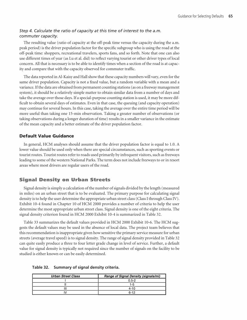
Step 4. Calculate the ratio of capacity at this time of interest to the a.m.commuter capacity.
The resulting value (ratio of capacity at the off-peak time versus the capacity during the a.m.peak period) is the driver population factor for the specific subgroup who is using the road at theoff-peak time: shoppers, recreational travelers, sports fans, and so forth. Note that one can alsouse different times of year (as Lu et al. did) to reflect varying tourist or other driver types of localconcern. All that is necessary is to be able to identify times when a section of the road is at capac-ity and compare that with the capacity observed for commuter traffic.
The data reported in Al-Kaisy and Hall show that these capacity numbers will vary, even for thesame driver population. Capacity is not a fixed value, but a random variable with a mean and avariance. If the data are obtained from permanent counting stations (as on a freeway managementsystem), it should be a relatively simple matter to obtain similar data from a number of days andtake the average over those days. If a special-purpose counting station is used, it may be more dif-ficult to obtain several days of estimates. Even in that case, the queuing (and capacity operation)may continue for several hours. In this case, taking the average over the entire time period will bemore useful than taking one 15-min observation. Taking a greater number of observations (ortaking observations during a longer duration of time) results in a smaller variance in the estimateof the mean capacity and a better estimate of the driver population factor.
Default Value Guidance
In general, HCM analyses should assume that the driver population factor is equal to 1.0. Alower value should be used only when there are special circumstances, such as sporting events ortourist routes. Tourist routes refer to roads used primarily by infrequent visitors, such as freewaysleading to some of the western National Parks. The term does not include freeways to or in resortareas where most drivers are regular users of the road.
Signal Density on Urban Streets
Signal density is simply a calculation of the number of signals divided by the length (measuredin miles) on an urban street that is to be evaluated. The primary purpose for calculating signaldensity is to help the user determine the appropriate urban street class (Class I through Class IV).Exhibit 10-4 found in Chapter 10 of HCM 2000 provides a number of criteria to help the userdetermine the most appropriate urban street class. Signal density is one of the eight criteria. Thesignal density criterion found in HCM 2000 Exhibit 10-4 is summarized in Table 32.
Table 33 summarizes the default values provided in HCM 2000 Exhibit 10-6. The HCM sug-gests the default values may be used in the absence of local data. The project team believes thatthis recommendation is inappropriate given how sensitive the primary service measure for urbanstreets (average travel speed) is to signal density. The range of signal density provided in Table 32can quite easily produce a three to four letter grade change in level of service. Further, a defaultvalue for signal density is typically not required since the number of signals on the facility to bestudied is either known or can be easily determined.
Guidance for Selecting Defaults 65
Urban Street Class Range of Signal Density (signals/mi) I 0.5-2II 1-5III 4-10IV 6-12
Table 32. Summary of signal density criteria.

Default Value Guidance
It is recommended that no default value for signal density be provided in future editions of theHCM. In situations where the number of signals along a facility is not known (potentially for long-range planning applications), it is recommended that the following guidance be used:
If the number of signals per mile is not known for a given planning application, it is recom-mended that the analyst first conduct a planning level assessment using a tool such as Exhibit10-15 in HCM 2000 (see Figure 18) to determine which intersections along the urban street arelikely to warrant signals.
Free-Flow Speed on Urban Streets
This section of the Guidebook describes a procedure for estimating the free-flow speed of anurban street. It is divided into four parts. The first part reviews current guidance contained in theHCM on free-flow speed. The second part summarizes research related to the free-flow speed forurban streets. The third part describes a procedure for estimating free-flow speed. The fourth partprovides guidance for estimating free-flow speed. Much of the work described herein is a prod-
66 Default Values for Highway Capacity and Level of Service Analyses
Urban Street Class Default Values (signals/mi) I 0.8II 3III 6IV 10
Table 33. Signal density default values.
EXHIBIT 10-15. INTERSECTION CONTROL TYPE AND PEAK-HOUR VOLUMES (SEE FOOTNOTE FOR ASSUMED VALUES)
Major Street Peak-Hour Two-Way Volume (veh/h) 0
0
100
200
300
400
500
600
700
800
200 400 600 800 1000 1200 1400 1600 1800 2000
Two-way stop TWSCa
All-way stop AWSCa
Traffic signal controla
Infeasible region minor > major
Min
or S
treet
Pea
k-H
our T
wo-
Way
Vol
ume
(veh
/h)
Notesa. Roundabouts may be appropriate within a portion of these ranges.Source: Adapted from Traffic Control Devices Handbook (8, pp. 4–18) - peak-direction, 8-h warrants converted to two-way peak-hour volumes assuming ADT equals twice the 8-h volume and peak hour is 10 percent of daily. Two-way volumes assumed to be 150 percent of peak-direction volume.
Figure 18. Intersection control type and peak-hour volumes.
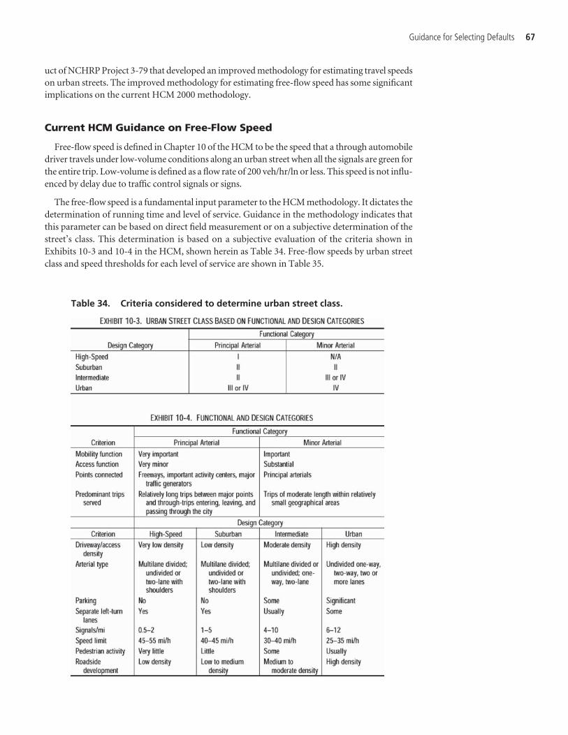
uct of NCHRP Project 3-79 that developed an improved methodology for estimating travel speedson urban streets. The improved methodology for estimating free-flow speed has some significantimplications on the current HCM 2000 methodology.
Current HCM Guidance on Free-Flow Speed
Free-flow speed is defined in Chapter 10 of the HCM to be the speed that a through automobiledriver travels under low-volume conditions along an urban street when all the signals are green forthe entire trip. Low-volume is defined as a flow rate of 200 veh/hr/ln or less. This speed is not influ-enced by delay due to traffic control signals or signs.
The free-flow speed is a fundamental input parameter to the HCM methodology. It dictates thedetermination of running time and level of service. Guidance in the methodology indicates thatthis parameter can be based on direct field measurement or on a subjective determination of thestreet’s class. This determination is based on a subjective evaluation of the criteria shown inExhibits 10-3 and 10-4 in the HCM, shown herein as Table 34. Free-flow speeds by urban streetclass and speed thresholds for each level of service are shown in Table 35.
Guidance for Selecting Defaults 67
Table 34. Criteria considered to determine urban street class.

Chapter 21 of the HCM describes a model for computing the free-flow speed for multilane high-ways. This model is based on the following equation:
Where
Sf = free-flow speed, mph;Sb = base free-flow speed (may use 47, 52, 55, or 60 for speed limits of 40, 45, 50, or 55, respec-
tively), mph;fLW = adjustment for lane width, mph;fLC = adjustment for lateral clearance, mph;fM = adjustment for median treatment, mph; andfA = adjustment for access points, mph.
The adjustment factors used in this equation indicate that lane width, lateral clearance, mediantype, and access point density can reduce the free-flow speed. The magnitude of the adjustmentsis listed in Table 36. Notably absent is an adjustment for heavy vehicles. This effect is accommo-dated as an adjustment to the analysis flow rate.
Summary of Relevance Research
This section examines the relationship between free-flow speed and two other variables:speed limit and segment length. It includes the guidance provided in the HCM (as describedin the previous section) as well as the guidance provided in three other sources. One sourcethat presents the relationship between free-flow speed and speed limit is Dowling et al. Thisresearch examined speed data from 10 speed measurement stations on four rural highways inthree states. The following relationship was developed between free-flow speed and speedlimit:
Where
Sf = free-flow speed, mph; andSpl = posted speed limit, mph.
A second source is the Florida Department of Transportation. The FDOT Quality/Level of Ser-vice Handbook indicates that the free-flow speed can be estimated as being 5 mph faster than theposted speed limit.
S Sf pl= +14
S S f f f ff b LW LC M A= − − − −
68 Default Values for Highway Capacity and Level of Service Analyses
Table 35. Level of service thresholds.

The guidance from Dowling et al., FDOT, and the HCM is summarized in Figure 19. The guid-ance provided in Chapter 10 of the HCM suggests that the free-flow speed is slightly slower thanthe speed limit. In contrast, FDOT, Chapter 21 of the HCM, and Dowling et al. suggest that thefree-flow speed is 5 to 7 mph faster than the speed limit. However, it must be remembered thatthe latter two sources are based on rural highway data.
A third source of insight into the relationship between free-flow speed and speed limit is the datacollected by Fitzpatrick et al. This database includes measurements of free-flow speed on 35 urban
Guidance for Selecting Defaults 69
Adjustment for Lateral Clearance
Four-Lane Highways Six-Lane Highways
Lateral Clearance, ft fLC, mph
Lateral Clearance, ft fLC, mph
12 0.0 12 0.0
10 0.4 10 0.4
8 0.9 8 0.9
6 1.3 6 1.3
4 1.8 4 1.7
2 3.6 2 2.8
0 5.4 0 3.9
Adjustment for Lane Width Adjustment for Access Point Density(right side only)
Lane Width, ft fLW, mphAccess
Density, ap/mi fA, mph
12 0.0 0 0.0
11 1.9 10 2.5
10 6.6 20 5.0
Adjustment for Median Treatment
30 7.5
Median Type fM, mph 40 10.0
Undivided 1.6
Divided 0.0
Table 36. Free-flow speed adjustment factors for multilane highways.
30
40
50
60
70
30 40 50
Speed Limit, mph
60 70
Fre
e-F
low
Sp
eed
, mp
h
HCM Chapter 10
HCM Chapter 21
Dowling et al.
FDOT
11
Figure 19. Comparison of guidance relating free-flow speed to speed limit.

or suburban arterial street segments in six states. The database collectively has segments ranging inlength from 0.4 to 1.0 mi; access point densities ranging from 0 to 103 per mi; speed limits rangingfrom 30 to 55 mph; lane widths ranging from 9.5 to 14.0 ft, and median types that included nomedian, non-restrictive, and restrictive.
The relationship between speed limit and free-flow speed on urban streets, as represented by thisequation is shown in Figure 20. The data points shown in the figure represent the data collected byFitzpatrick et al. The coefficient of determination (R2) for the model is 0.66, which implies that themodel explains 66% of the variability in the data.
The trends shown in Figure 20 indicate that free-flow speed is typically faster than the speedlimit. However, the relationship between the two speeds is not consistent with the guidancedescribed previously. This difference is partly due to the fact that speed limit is correlated withaccess point density—higher speed limits are associated with lower densities. The trend inFigure 20 also suggests that the free-flow speed and the speed limit tend to equal one anotherat a certain specific speed limit. Specifically, the trend suggests that the free-flow speed tendsto equal the speed limit of about 45 mph on urban arterial streets. The trend suggests thatdrivers are content with this speed limit when traveling on an arterial street. However, driverswill likely adopt a free-flow speed that is in excess of the speed limit if that limit is posted at alower value.
Exhibit 15-3 of HCM Chapter 15 provides a table of running time rates for urban street appli-cations. The trend in these rates suggests that speed is influenced by segment length. This effect oflength is inferred to affect all vehicles traveling along the segment. The implication of this inferenceis that free-flow speed is influenced by segment length.
The rates listed in Exhibit 15-3 of the HCM are shown in Figure 21, after conversion to an equiv-alent speed value. The trend lines converge to the stated free-flow speed at the right side of the fig-ure. Given that they converge to the free-flow speed and that length affects all vehicles, it is ration-alized that the designated “free-flow speed” to which the rates converge on long segments is actuallyan “ideal free-flow speed.” In this context, the “ideal free-flow speed” is defined to be the free-flowspeed on long street segments such that the potential need to stop at the next signal does nothave to be factored into the driver’s speed choice. Thus, ideal free-flow speed can only be field-measured on long street segments. It is an abstract concept for short segments and can only be esti-mated through the use of a mathematical relationship. For example, if the field-measured free-flowspeed on a Class 1 street with a length of 0.4 mi is 44 mph, then the trend lines in Figure 21 indi-
70 Default Values for Highway Capacity and Level of Service Analyses
20
30
40
50
60
20 30 40 50 60 70
Speed Limit, mph
Fre
e-F
low
Sp
eed
, mp
h
11
Figure 20. Relationship between speed limit and free-flow speed.
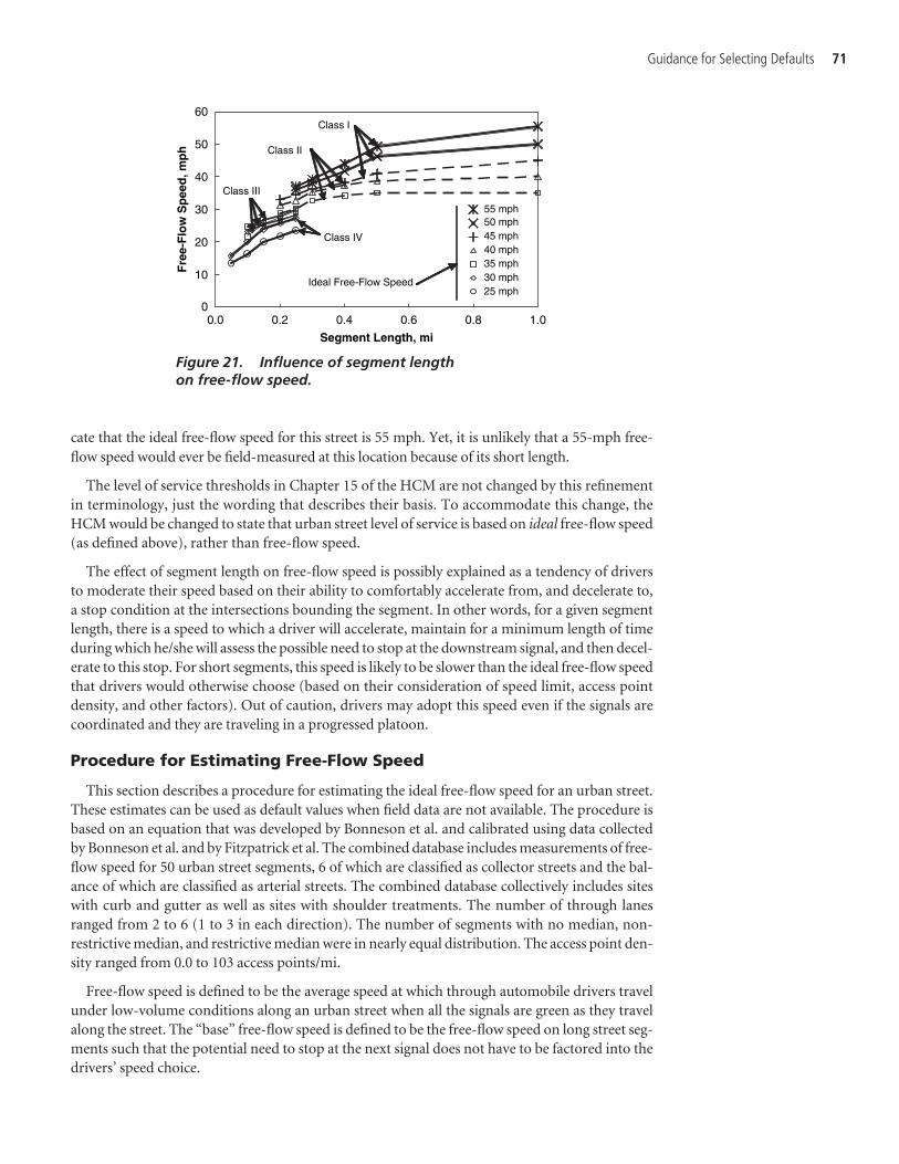
cate that the ideal free-flow speed for this street is 55 mph. Yet, it is unlikely that a 55-mph free-flow speed would ever be field-measured at this location because of its short length.
The level of service thresholds in Chapter 15 of the HCM are not changed by this refinementin terminology, just the wording that describes their basis. To accommodate this change, theHCM would be changed to state that urban street level of service is based on ideal free-flow speed(as defined above), rather than free-flow speed.
The effect of segment length on free-flow speed is possibly explained as a tendency of driversto moderate their speed based on their ability to comfortably accelerate from, and decelerate to,a stop condition at the intersections bounding the segment. In other words, for a given segmentlength, there is a speed to which a driver will accelerate, maintain for a minimum length of timeduring which he/she will assess the possible need to stop at the downstream signal, and then decel-erate to this stop. For short segments, this speed is likely to be slower than the ideal free-flow speedthat drivers would otherwise choose (based on their consideration of speed limit, access pointdensity, and other factors). Out of caution, drivers may adopt this speed even if the signals arecoordinated and they are traveling in a progressed platoon.
Procedure for Estimating Free-Flow Speed
This section describes a procedure for estimating the ideal free-flow speed for an urban street.These estimates can be used as default values when field data are not available. The procedure isbased on an equation that was developed by Bonneson et al. and calibrated using data collectedby Bonneson et al. and by Fitzpatrick et al. The combined database includes measurements of free-flow speed for 50 urban street segments, 6 of which are classified as collector streets and the bal-ance of which are classified as arterial streets. The combined database collectively includes siteswith curb and gutter as well as sites with shoulder treatments. The number of through lanesranged from 2 to 6 (1 to 3 in each direction). The number of segments with no median, non-restrictive median, and restrictive median were in nearly equal distribution. The access point den-sity ranged from 0.0 to 103 access points/mi.
Free-flow speed is defined to be the average speed at which through automobile drivers travelunder low-volume conditions along an urban street when all the signals are green as they travelalong the street. The “base” free-flow speed is defined to be the free-flow speed on long street seg-ments such that the potential need to stop at the next signal does not have to be factored into thedrivers’ speed choice.
Guidance for Selecting Defaults 71
0
10
20
30
40
50
60
0.0 0.2 0.4 0.6 0.8 1.0
Segment Length, mi
Fre
e-F
low
Sp
eed
, mp
h
55 mph50 mph45 mph40 mph35 mph30 mph25 mph
Class II
Class I
Class III
Class IV
Ideal Free-Flow Speed
Figure 21. Influence of segment length on free-flow speed.
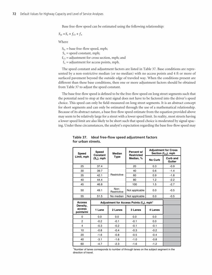
Base free-flow speed can be estimated using the following relationship:
Where
Sfo = base free-flow speed, mph;So = speed constant, mph;fCS = adjustment for cross section, mph; andfA = adjustment for access points, mph.
The speed constant and adjustment factors are listed in Table 37. Base conditions are repre-sented by a non-restrictive median (or no median) with no access points and 4 ft or more ofsurfaced pavement beyond the outside edge of traveled way. When the conditions present aredifferent than these base conditions, then one or more adjustment factors should be obtainedfrom Table 37 to adjust the speed constant.
The base free-flow speed is defined to be the free-flow speed on long street segments such thatthe potential need to stop at the next signal does not have to be factored into the driver’s speedchoice. This speed can only be field-measured on long street segments. It is an abstract conceptfor short segments and can only be estimated through the use of a mathematical relationship.Because of its abstract nature, a base free-flow speed estimate from the equation provided abovemay seem to be relatively large for a street with a lower speed limit. In reality, most streets havinga lower speed limit are also likely to be short such that speed choice is moderated by signal spac-ing. Under these circumstances, the analyst’s expectation regarding the base free-flow speed may
S S f ffo o CS A= + +
72 Default Values for Highway Capacity and Level of Service Analyses
Table 37. Ideal free-flow speed adjustment factors for urban streets.
Adjustment for Cross Section (fCS), mphSpeed
Limit, mph
SpeedConstant (So), mph
MedianType
Percent w/RestrictedMedian, % No Curb Curb and
Gutter
25 37.4 20 0.3 -0.9
30 39.7 40 0.6 -1.4
35 42.1 60 0.9 -1.8
40 44.4 80 1.2 -2.2
45 46.8
Restrictive
100 1.5 -2.7
50 49.1 Non-Restrictive Not applicable 0.0 -0.5
55 51.5 No median Not applicable 0.0 -0.5
Adjustment for Access Points (fA), mph1AccessDensity, access
points/mi 1 Lane 2 Lanes 3 Lanes 4 Lanes
0 0.0 0.0 0.0 0.0
2 -0.2 -0.1 -0.1 0.0
4 -0.3 -0.2 -0.1 -0.1
10 -0.8 -0.4 -0.3 -0.2
20 -1.6 -0.8 -0.5 -0.4
40 -3.1 -1.6 -1.0 -0.8
60 -4.7 -2.3 -1.6 -1.2
1Number of lanes corresponds to number of through lanes on the subject segment in thedirection of travel.
be skewed because what has actually been observed at this location is free-flow speed (not the basefree-flow speed), as influenced by segment length.
Default Value Guidance
HCM 2000 has one simple table of default values for free-flow speed (HCM 2000 Exhibit 10-5).For each of the four classes of urban streets there is a recommended default value for free-flowspeed. These default values are also what define the level of service thresholds shown in HCM 2000Exhibit 15-2.
The methodology presented in this Guidebook requires more than a simple replacement ofExhibit 10-5. Rather than develop default free-flow speed estimates, use of the equation on thepreceding page should be considered.
Saturation Flow Rates and Lane Utilization Factors for Dual and Triple Left-Turn Lanes
This section focuses on HCM procedures for determining the saturation flow rate and laneutilization factors for use in the analysis of signalized intersection operations for signalized inter-sections with dual and triple left-turn lanes. Recommended values provided in other researchstudies are summarized.
The current default value for a saturation flow rate for a single left-turn lane is 1,805. Thissaturation flow rate default value is derived by multiplying the base saturation flow rate of1,900 by 95%, as shown in Equation 16-7 in the HCM. No saturation flow rate default valueis given in the HCM for dual or triple left-turn lanes. The current default value for the laneutilization adjustment factor for dual left-turn lanes is 0.971, as found in Exhibit 10-23 in theHCM. No lane utilization default value exists for triple left-turn lanes. The HCM provides anoption for 0.971 to be used as a default value for triple left-turn lanes; however, a survey oflocal conditions is preferred.
HCM 2000 Procedures
The HCM provides methodologies for determining the saturation flow rate and lane utiliza-tion factors for dual and triple left-turn lanes for signalized intersections. A summary of the equa-tions which consider these values is provided below. Chapter 16 outlines the methodology foranalyzing signalized intersections. This methodology includes the determination of the satura-tion flow rate. The equation for this calculation is shown below:
Where
s = saturation flow rate for subject lane group, expressed as a total for all lanes in lane group(veh/h);
so = base saturation flow rate per lane (pc/hr/ln);N = number of lanes in lane group;fw = adjustment factor for lane width;
fHV = adjustment factor for heavy vehicles in traffic stream;fg = adjustment factor for approach grade;fp = adjustment factor for existence of a parking lane and parking activity adjacent to lane
group;fbb = adjustment factor for blocking effect of local buses that stop within intersection area;
s s Nf f f f f f f f f f fo w HV g p bb a LU LT RT Lpb Rpb=
Guidance for Selecting Defaults 73
fa = adjustment factor for area type;fLU = adjustment factor for lane utilization;fLT = adjustment factor for left turns in lane group;fRT = adjustment factor for right turns in lane group;fLpb = pedestrian adjustment factor for left-turn movements; andfRpb = pedestrian-bicycle adjustment factor for right-turn movements.
As shown in the above equation, the adjustment factor for left turns in a lane group and theadjustment factor for lane utilization are two of the eleven adjustment factors used in calculat-ing the saturation flow rate for the subject lane group.
The adjustment factor for left turns in lane group is calculated using the following equations(found in Exhibit 16-7):
Where
PLT = proportion of left turns in lane group
The equation for determining the adjustment for lane utilization is found in Exhibit 16-5:
Where
fLU = lane utilization adjustment factor,
vg = unadjusted demand flow rate for lane group (veh/hr),vg1 = unadjusted demand flow rate on single lane with highest volume in lane group (veh/hr),
andN = number of lanes in lane group.
Summary of Relevant Research
Six research studies were reviewed with respect to procedures for determining the saturationflow rate and lane utilization factors for analysis of intersections with multiple left-turn lanes. Asummary of these research studies is provided below.
Spring, G. S., and Thomas, A. Double Left-Turn Lanes in Medium-Size Cities. Journal of Trans-portation Engineering, Vol. 125, March/April 1999, pp. 138–143.
Double left-turn data from 30 intersections in the city of Greensboro, North Carolina, wereanalyzed with respect to relationships among performance and geometric characteristics. Resultsindicated that the overall saturation flow left-turn adjustment value of 0.92, recommended bythe 1985 HCM, appears reasonable for the inside (curb) lane. Values of 0.86 to 0.88 are moreappropriate for the outside (farthest from median) lane adjustments. A single left-turn factor of0.92 is recommended for dual left-turn approaches where the turn angle is very close to 90° andwhere the intersection functions as a T-intersection (i.e., no opposing flow), or where the turnangle for a four-leg intersection is less than 90°. Separate left-turn factors for each of the two left-turn lanes are recommended at all other dual left-turn lane approaches. Lane utilization factorswere not discussed.
fv
v NLU
g
g
= ( )1
Exclusive Lane:
Shared Lane:1
1.0
f
f
LT
LT
=
=
0 95.
++ 0.05 PLT
74 Default Values for Highway Capacity and Level of Service Analyses
Zegeer, J. D. Field Validation of Intersection Capacity Factors. Transportation Research RecordNo. 1091, 1986, pp. 67–77.
The purpose of this study was to verify the saturation flow rates and traffic volume adjustmentfactors used in various capacity analysis procedures by assembling a relatively extensive database.Saturation flow headways were collected for more than 20,000 headways around the UnitedStates. Results indicated that left-turning vehicles in saturation flow at single left-turn lanes expe-rienced an average of 3% reduction in saturation flow rate when compared with through-laneheadways at comparable locations. Therefore, a 0.97 adjustment factor for single left-turn lanesis recommended. For dual left-turn lanes, results indicated that 50.3% of the vehicles surveyedwere in the inside (curb) lane. The lane distribution suggests a lane utilization factor of 0.97 forthe dual left-turn lane, when compared with single exclusive left-turn lanes. Combining the sin-gle and dual turn lane adjustment factors for protected turn phase operations yields an overallfactor that can be applied to unadjusted turn volumes in dual exclusive turn lanes. The overalladjustment factor of 0.94 for a dual left-turn lane was recommended.
Kagolanu, K., and Szplett, D. Saturation Flow Rates of Dual Left-Turn Lanes. Proc., Second Inter-national Symposium on Highway Capacity, Akcelik, R. (ed.), Volume 1, 1994, pp. 325–344.
This paper studied the saturation flow headways in the inside and outside dual left-turn lanes,distribution in lanes, and effects of striping and geometry. A total of 2,359 headways were collectedand subjected to statistical analyses from sites in Boise, Idaho. Results indicated that left-turn laneuse is 46% for the inside (curb) lane and 54% for the outside lane. Using the lane utilization factorvalue equation presented earlier, a lane utilization factor value of 0.89 is calculated. The average sat-uration flow rate calculated using the mean of the headways was 1,640 for the inside (curb) lane and1,691 for the outside lane. Because the observed saturation flow rate was not corrected for otheradjustment factors, it is inappropriate to compute a left-turn adjustment factor. The study also sug-gested that the striping and receiving lanes may factor into the observed saturation flow rates.
Stokes, R. W., Messer, C. J., and Stover, V. G. Saturation Flows of Exclusive Double Left-TurnLanes. Transportation Research Record No. 1091, 1986, pp. 86–95.
This paper developed estimates of the saturation flows at exclusive double left-turn lanes. Theresults are based on observations of 3,458 completed left turns from exclusive double left-turn laneson 14 intersections in Austin, College Station, and Houston, Texas. Results indicated that the aver-age double left-turn saturation flow rate varied by city. An average saturation flow rate for doubleleft-turn lanes of 1,636, 1,636, and 1,800 was found in Austin, College Station, and Houston,respectively. The study also concluded that any differences in the departure headways used to cal-culate saturation flow for vehicles in the inside (curb) lane, and outside lane are not large enoughto be detected with the given sample sizes. The paper made no recommendations for a left-turnadjustment factor or lane utilization factor due to the inconsistency of the results.
Leonard II, J. D. Operational Characteristics of Triple Left Turns. Transportation Research RecordNo. 1457, 1994, pp. 104–110.
This paper studied the characteristics of triple left turns using five triple left-turn sites in OrangeCounty, California. A sample consisting of 4,742 lane cycles was compiled for analysis. Resultsindicate that the average saturation flow rate observed was 1,930. A left-turn adjustment factorwas not recommended due to the limited number of survey locations. Lane utilization factors of1.01 for the inside (curb)/middle lane group and 0.98 for the outer lane group were computed.
Sando, T., and Mussa, R. N. Site Characteristics Affecting Operation of Triple Left-Turn Lanes.Transportation Research Record No. 1457, 1994, pp. 104–110.
This study analyzed the influence of a number of geometric factors found at 15 triple left-turnlane sites in Florida on saturation flow rate and lane utilization. A total of 2,395 lane cycles were
Guidance for Selecting Defaults 75

observed. Results indicated that the average saturation flow rate observed was 1,859. Left-turnfactors of 0.91 and 0.92 were calculated for two intersections; however, due to the small samplesize, these values were not analyzed for statistical significance. An overall average lane utilizationfactor of 0.88 was calculated. A review of the data showed that lane usage is dependent on theintersection geometric configuration.
Default Value Guidance
This section of the Guidebook focused on HCM procedures for determining the saturationflow rate and lane utilization factors for use in the analysis of intersection operations for locationswith multiple left-turn lanes. Research studies have recommended varying left-turn adjustmentfactors and lane utilization factors for use with dual and triple left-turn lanes as summarized inTable 38.
It can be concluded that there are no universally accepted values for left-turn lane adjustmentfactors or lane utilization factors. Although local data will provide the truest measure of theappropriate adjustment factors at a location, these data are typically not collected due to projectbudget and time constraints. When local data are not available, the following default values maybe considered:
Left-Turn Lane Saturation Flow Adjustment Factor (Dual Left-Turn Lanes)• Set the default value to 0.97.Left-Turn Lane Utilization Factor (Dual Left-Turn Lanes)• Maintain the current default value of 0.971 as suggested by the HCM.Left-Turn Lane Saturation Flow Adjustment Factor (Triple Left-Turn Lanes)• Set the default value to 0.97 until research can be completed.Left-Turn Lane Utilization Factor (Triple Left-Turn Lanes)• Set the default value to 0.971 as suggested by the HCM until further research is available.
Caution: Lane utilization values can be significantly influenced by the presence of freeway rampslocated downstream of the intersection.
76 Default Values for Highway Capacity and Level of Service Analyses
Dual Left-Turn Lanes Triple Left-Turn Lanes
Source LTf LUf LTf LUf
Highway Capacity Manual -- 0.971 -- 0.971
Double Left-Turn Lanes in Medium-Size Cities, Spring
0.92Inside(curb)
0.86-0.88Outside
-- -- --
Field Validation of Intersection Capacity Factors, Zegeer
0.97 0.97 -- --
Saturation Flow Rates of Dual Left-Turn Lanes, Kagolanu
-- 0.89 -- --
Operational Characteristics of Triple Left Turns, Leonard
-- -- -- 1.01Inside (curb)/ Middle
0.98Outside
Site Characteristics Affecting Operation of Triple Left-Turn Lanes,Sando
-- -- -- 0.88
Table 38. Summary of left-turn factors by source.
A service volume table can provide an analyst with an estimate of the maximum number of vehi-cles a facility can carry at a given Level of Service. The use of a service volume table is most appro-priate in certain planning applications where it is not feasible to evaluate every segment or nodewithin a study area. Examples of this would be city, county, or statewide planning studies wherethe size of the study area makes it infeasible to conduct a capacity or level of service analysis forevery roadway segment. For these types of planning applications, the focus of the effort is to sim-ply highlight “potential” problem areas (e.g., locations where demand may exceed capacity orwhere a desired level of service threshold may be exceeded). For such applications, developing aservice volume table can be a useful sketch planning tool, provided the analyst understands thelimitations of this method.
To develop a service volume table, the analyst needs to develop a default value for each of theinput parameters. As discussed in previous chapters of this Guidebook, several of the default val-ues have a very significant impact on the resulting level of service. For this reason, great care shouldbe used when developing a set of default values that the analyst believes is most appropriate for thelocal condition. Further, when applying the service volume table, it is important to recognize thatthe various roadway segments being evaluated are not likely to have the exact values for all the inputparameters. Accordingly, conclusions drawn from the application of service volume tables shouldbe considered and presented as “rough approximations.”
Sample Service Volume Tables
For the purposes of this Guidebook, an example of how to construct a service volume table wasprepared for a basic freeway segment and for an urban street facility. These two facility types wereselected since they would likely be common applications of service volume tables within an urbanarea. The tables presented below were developed for illustrative purposes only. The analyst should care-fully select default values that are most appropriate for the local condition.
Basic Freeway Segment Example
For the basic freeway segment example, Table 39 was prepared based on the followingassumed default values:
• Base free-flow speed: 70 mph• Lane width: 12 ft• Shoulder width: 6 ft• Terrain: level• %HV: 5
77
C H A P T E R 5
Guidance for Preparing Service Volume Tables
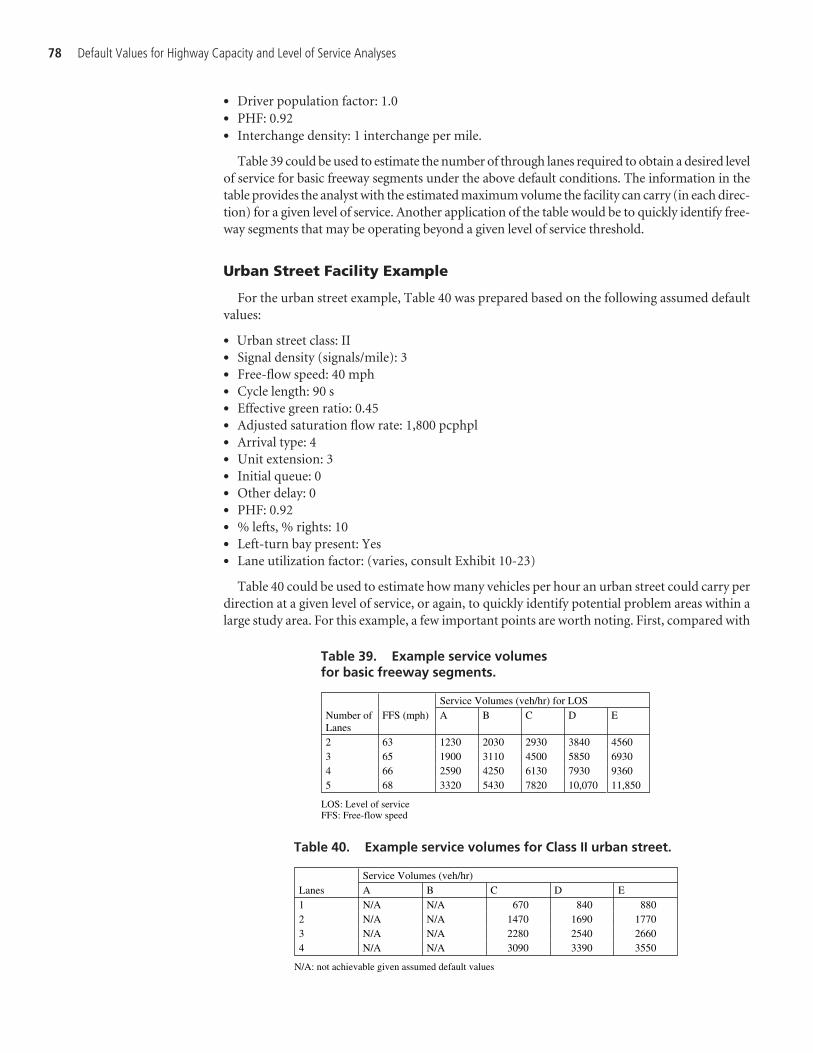
• Driver population factor: 1.0• PHF: 0.92• Interchange density: 1 interchange per mile.
Table 39 could be used to estimate the number of through lanes required to obtain a desired levelof service for basic freeway segments under the above default conditions. The information in thetable provides the analyst with the estimated maximum volume the facility can carry (in each direc-tion) for a given level of service. Another application of the table would be to quickly identify free-way segments that may be operating beyond a given level of service threshold.
Urban Street Facility Example
For the urban street example, Table 40 was prepared based on the following assumed defaultvalues:
• Urban street class: II• Signal density (signals/mile): 3• Free-flow speed: 40 mph• Cycle length: 90 s• Effective green ratio: 0.45• Adjusted saturation flow rate: 1,800 pcphpl• Arrival type: 4• Unit extension: 3• Initial queue: 0• Other delay: 0• PHF: 0.92• % lefts, % rights: 10• Left-turn bay present: Yes• Lane utilization factor: (varies, consult Exhibit 10-23)
Table 40 could be used to estimate how many vehicles per hour an urban street could carry perdirection at a given level of service, or again, to quickly identify potential problem areas within alarge study area. For this example, a few important points are worth noting. First, compared with
78 Default Values for Highway Capacity and Level of Service Analyses
Table 39. Example service volumes for basic freeway segments.
Table 40. Example service volumes for Class II urban street.
Service Volumes (veh/hr) for LOSNumber ofLanes
FFS (mph) A B C D E
2 63 1230 2030 2930 3840 4560 3 65 1900 3110 4500 5850 6930 4 66 2590 4250 6130 7930 9360 5 68 3320 5430 7820 10,070 11,850
LOS: Level of service FFS: Free-flow speed
Service Volumes (veh/hr) Lanes A B C D E 1 N/A N/A 670 840 880 2 N/A N/A 1470 1690 1770 3 N/A N/A 2280 2540 2660 4 N/A N/A 3090 3390 3550
N/A: not achievable given assumed default values
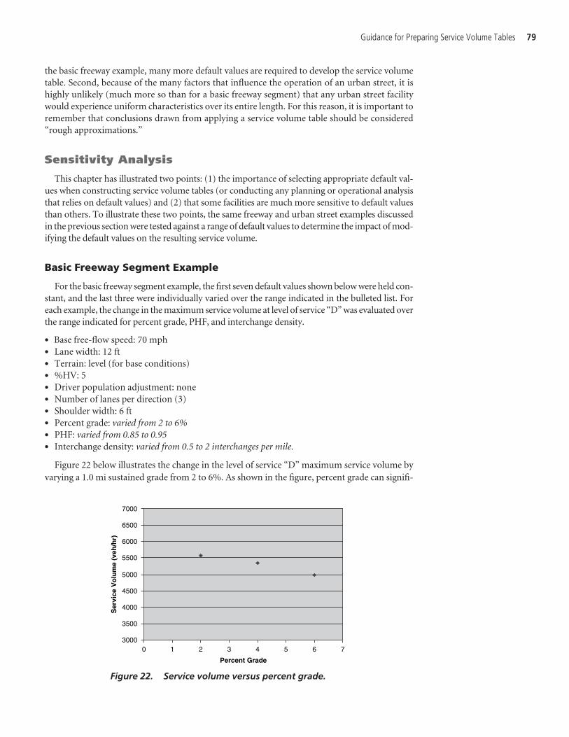
the basic freeway example, many more default values are required to develop the service volumetable. Second, because of the many factors that influence the operation of an urban street, it ishighly unlikely (much more so than for a basic freeway segment) that any urban street facilitywould experience uniform characteristics over its entire length. For this reason, it is important toremember that conclusions drawn from applying a service volume table should be considered“rough approximations.”
Sensitivity Analysis
This chapter has illustrated two points: (1) the importance of selecting appropriate default val-ues when constructing service volume tables (or conducting any planning or operational analysisthat relies on default values) and (2) that some facilities are much more sensitive to default valuesthan others. To illustrate these two points, the same freeway and urban street examples discussedin the previous section were tested against a range of default values to determine the impact of mod-ifying the default values on the resulting service volume.
Basic Freeway Segment Example
For the basic freeway segment example, the first seven default values shown below were held con-stant, and the last three were individually varied over the range indicated in the bulleted list. Foreach example, the change in the maximum service volume at level of service “D” was evaluated overthe range indicated for percent grade, PHF, and interchange density.
• Base free-flow speed: 70 mph• Lane width: 12 ft• Terrain: level (for base conditions)• %HV: 5• Driver population adjustment: none• Number of lanes per direction (3)• Shoulder width: 6 ft• Percent grade: varied from 2 to 6%• PHF: varied from 0.85 to 0.95• Interchange density: varied from 0.5 to 2 interchanges per mile.
Figure 22 below illustrates the change in the level of service “D” maximum service volume byvarying a 1.0 mi sustained grade from 2 to 6%. As shown in the figure, percent grade can signifi-
Guidance for Preparing Service Volume Tables 79
Figure 22. Service volume versus percent grade.
3000
3500
4000
4500
5000
5500
6000
6500
7000
0 1 2 3 4 5 6 7
Percent Grade
Ser
vice
Vo
lum
e (v
eh/h
r)
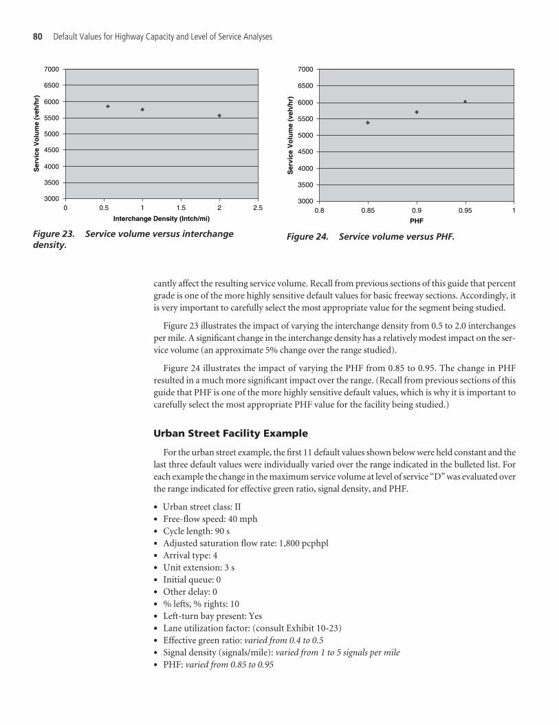
cantly affect the resulting service volume. Recall from previous sections of this guide that percentgrade is one of the more highly sensitive default values for basic freeway sections. Accordingly, itis very important to carefully select the most appropriate value for the segment being studied.
Figure 23 illustrates the impact of varying the interchange density from 0.5 to 2.0 interchangesper mile. A significant change in the interchange density has a relatively modest impact on the ser-vice volume (an approximate 5% change over the range studied).
Figure 24 illustrates the impact of varying the PHF from 0.85 to 0.95. The change in PHFresulted in a much more significant impact over the range. (Recall from previous sections of thisguide that PHF is one of the more highly sensitive default values, which is why it is important tocarefully select the most appropriate PHF value for the facility being studied.)
Urban Street Facility Example
For the urban street example, the first 11 default values shown below were held constant and thelast three default values were individually varied over the range indicated in the bulleted list. Foreach example the change in the maximum service volume at level of service “D” was evaluated overthe range indicated for effective green ratio, signal density, and PHF.
• Urban street class: II• Free-flow speed: 40 mph• Cycle length: 90 s• Adjusted saturation flow rate: 1,800 pcphpl• Arrival type: 4• Unit extension: 3 s• Initial queue: 0• Other delay: 0• % lefts, % rights: 10• Left-turn bay present: Yes• Lane utilization factor: (consult Exhibit 10-23)• Effective green ratio: varied from 0.4 to 0.5• Signal density (signals/mile): varied from 1 to 5 signals per mile• PHF: varied from 0.85 to 0.95
80 Default Values for Highway Capacity and Level of Service Analyses
Figure 23. Service volume versus interchangedensity.
Figure 24. Service volume versus PHF.
3000
3500
4000
4500
5000
5500
6000
6500
7000
0 0.5 1 1.5 2 2.5
Interchange Density (Intch/mi)
Ser
vice
Vo
lum
e (v
eh/h
r)
3000
3500
4000
4500
5000
5500
6000
6500
7000
0.8 0.85 0.9 0.95 1
PHF
Ser
vice
Vo
lum
e (v
eh/h
r)
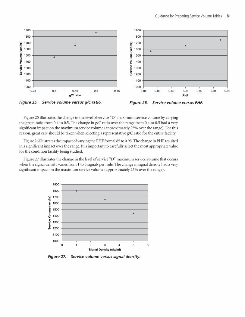
Guidance for Preparing Service Volume Tables 81
Figure 25. Service volume versus g/C ratio.
1000
1100
1200
1300
1400
1500
1600
1700
1800
1900
0.35 0.4 0.45 0.5 0.55
g/C ratio
Ser
vice
Vo
lum
e (v
eh/h
r)
Figure 25 illustrates the change in the level of service “D” maximum service volume by varyingthe green ratio from 0.4 to 0.5. The change in g/C ratio over the range from 0.4 to 0.5 had a verysignificant impact on the maximum service volume (approximately 25% over the range). For thisreason, great care should be taken when selecting a representative g/C ratio for the entire facility.
Figure 26 illustrates the impact of varying the PHF from 0.85 to 0.95. The change in PHF resultedin a significant impact over the range. It is important to carefully select the most appropriate valuefor the condition facility being studied.
Figure 27 illustrates the change in the level of service “D” maximum service volume that occurswhen the signal density varies from 1 to 5 signals per mile. The change in signal density had a verysignificant impact on the maximum service volume (approximately 25% over the range).
Figure 26. Service volume versus PHF.
1000
1100
1200
1300
1400
1500
1600
1700
1800
1900
0.84 0.86 0.88 0.9 0.92 0.94 0.96
PHF
Ser
vice
Vo
lum
e (v
eh/h
r)
Figure 27. Service volume versus signal density.
1000
1100
1200
1300
1400
1500
1600
1700
1800
1900
0 1 2 3 4 5 6
Signal Density (sig/mi)
Ser
vice
Vo
lum
e (v
eh/h
r)

83
A sensitivity analysis was conducted for all input parameters where HCM 2000 suggests defaultvalues. The intent of this analysis was to determine which input parameters deserved further studybased on the relative change in the relevant service measure due to the change in the value of theinput parameter. Those input parameters that had a high degree of impact on the relevant servicemeasures were recommended for further study. Input parameters considered for the sensitivityanalysis were those that the HCM 2000 has suggested default values for. Specifically, default valuesare suggested for 63 input parameters described in eight chapters of Part II of HCM 2000: UrbanStreets, Signalized Intersections, Pedestrians, Bicycles, Multilane Highways, Two-Lane Highways,Basic Freeway Segments, and Ramps and Ramp Junctions.
To facilitate the ranking of the input parameters, the following three thresholds were established.
• If varying the input parameter within its reasonable range results in 0 to 10% change in the ser-vice measure, the parameter is considered to have a low degree of sensitivity.
• If varying the input parameter within its reasonable range results in 10 to 20% change in theservice measure, the parameter is considered to have a moderate degree of sensitivity.
• If varying the input parameter within its reasonable range results in more than 20% change inthe service measure, the parameter is considered to have a high degree of sensitivity.
In general, input parameters that demonstrated a moderate to high degree of sensitivity wereconsidered for further investigation. The HiCAP software was used to determine how the varia-tion in input parameter values influenced the level of service for each of these methodologies.
Urban Streets
In the Urban Streets methodology, HCM 2000 provides default values for two input parame-ters: free-flow speed and signal density. (See Table A-1.) In each of four street classifications, adefault value is provided. Thus, a separate set of sensitivity analyses was developed correspondingto each of the four street classifications. The effects of free-flow speed and signal density on the ser-vice measure (and the level-of-service) were evaluated under low, average, and high traffic volumeconditions. Each sensitivity analysis began with the establishment of a base scenario, and input val-ues for the target parameter were varied to record its effects.
A summary of the base scenario is described in the following section.
Base Scenario
A set of base parameters was selected for determining the sensitivity of each of the two inputparameters listed above. These parameters represent the typical characteristics of an urban street
Sensitivity Analysis
A P P E N D I X A
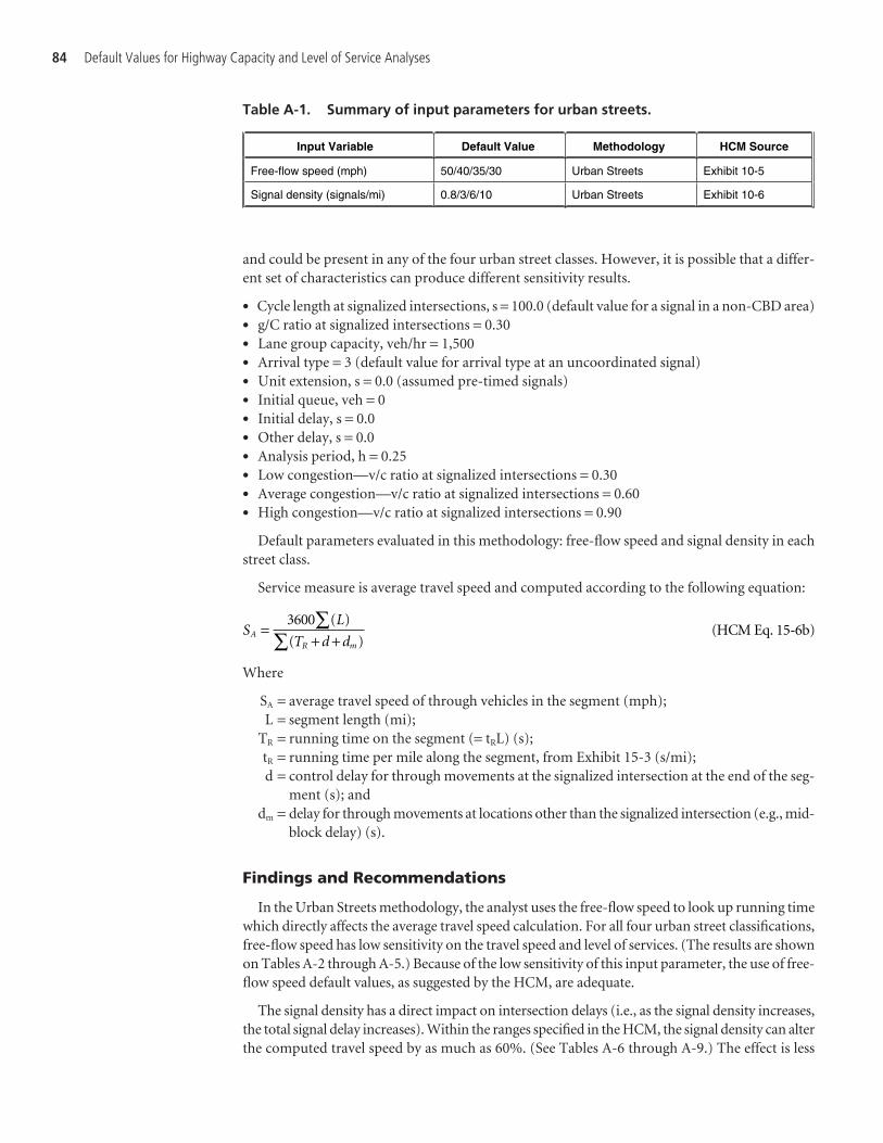
84 Default Values for Highway Capacity and Level of Service Analyses
and could be present in any of the four urban street classes. However, it is possible that a differ-ent set of characteristics can produce different sensitivity results.
• Cycle length at signalized intersections, s = 100.0 (default value for a signal in a non-CBD area)• g/C ratio at signalized intersections = 0.30• Lane group capacity, veh/hr = 1,500• Arrival type = 3 (default value for arrival type at an uncoordinated signal)• Unit extension, s = 0.0 (assumed pre-timed signals)• Initial queue, veh = 0• Initial delay, s = 0.0• Other delay, s = 0.0• Analysis period, h = 0.25• Low congestion—v/c ratio at signalized intersections = 0.30• Average congestion—v/c ratio at signalized intersections = 0.60• High congestion—v/c ratio at signalized intersections = 0.90
Default parameters evaluated in this methodology: free-flow speed and signal density in eachstreet class.
Service measure is average travel speed and computed according to the following equation:
Where
SA = average travel speed of through vehicles in the segment (mph);L = segment length (mi);
TR = running time on the segment (= tRL) (s);tR = running time per mile along the segment, from Exhibit 15-3 (s/mi);d = control delay for through movements at the signalized intersection at the end of the seg-
ment (s); anddm = delay for through movements at locations other than the signalized intersection (e.g., mid-
block delay) (s).
Findings and Recommendations
In the Urban Streets methodology, the analyst uses the free-flow speed to look up running timewhich directly affects the average travel speed calculation. For all four urban street classifications,free-flow speed has low sensitivity on the travel speed and level of services. (The results are shownon Tables A-2 through A-5.) Because of the low sensitivity of this input parameter, the use of free-flow speed default values, as suggested by the HCM, are adequate.
The signal density has a direct impact on intersection delays (i.e., as the signal density increases,the total signal delay increases). Within the ranges specified in the HCM, the signal density can alterthe computed travel speed by as much as 60%. (See Tables A-6 through A-9.) The effect is less
SL
T d dA
R m
=+ +∑
∑3600 ( )
( )(HCM Eq. 15-6b)
Input Variable Default Value Methodology HCM Source
Free-flow speed (mph) 50/40/35/30 Urban Streets Exhibit 10-5
Signal density (signals/mi) 0.8/3/6/10 Urban Streets Exhibit 10-6
Table A-1. Summary of input parameters for urban streets.
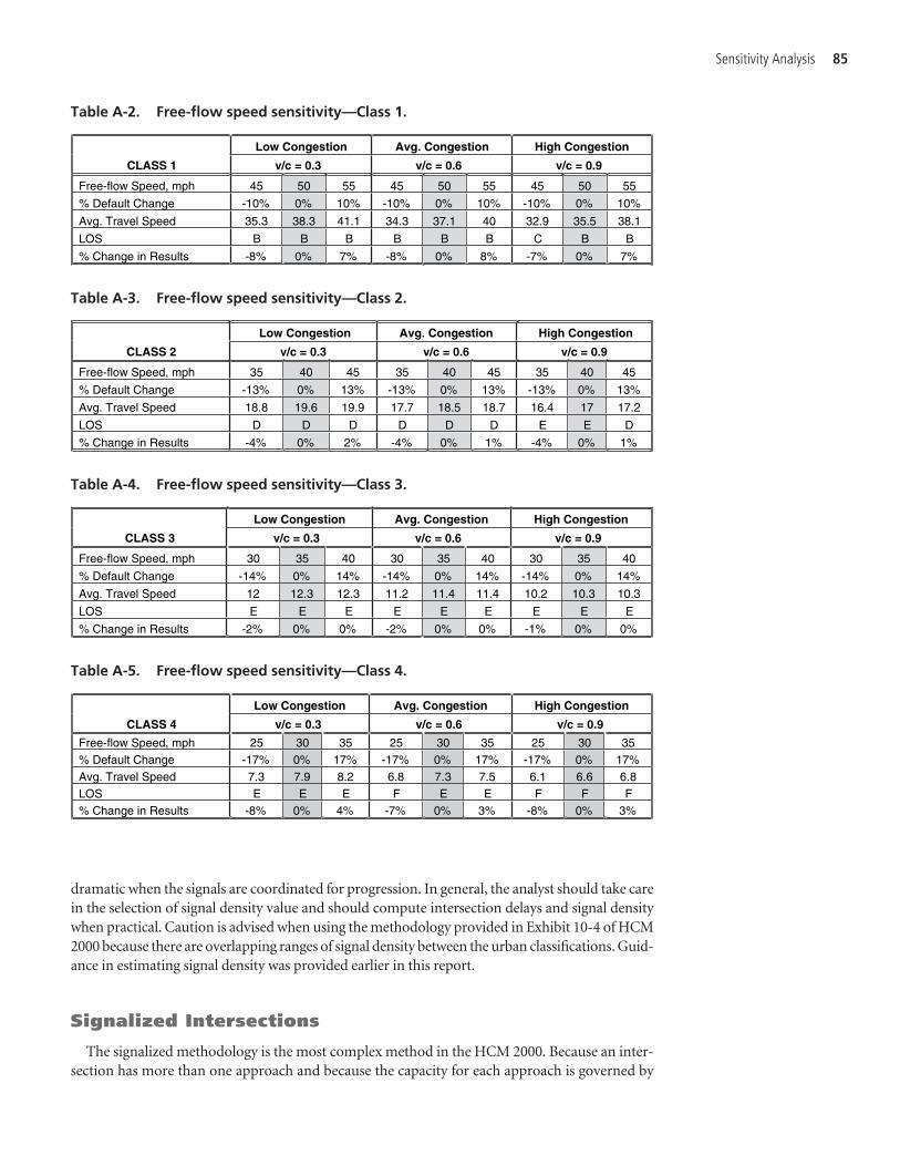
Sensitivity Analysis 85
dramatic when the signals are coordinated for progression. In general, the analyst should take carein the selection of signal density value and should compute intersection delays and signal densitywhen practical. Caution is advised when using the methodology provided in Exhibit 10-4 of HCM2000 because there are overlapping ranges of signal density between the urban classifications. Guid-ance in estimating signal density was provided earlier in this report.
Signalized Intersections
The signalized methodology is the most complex method in the HCM 2000. Because an inter-section has more than one approach and because the capacity for each approach is governed by
Low Congestion Avg. Congestion High Congestion
CLASS 2 v/c = 0.3 v/c = 0.6 v/c = 0.9
Free-flow Speed, mph 35 40 45 35 40 45 35 40 45
% Default Change -13% 0% 13% -13% 0% 13% -13% 0% 13%
Avg. Travel Speed 18.8 19.6 19.9 17.7 18.5 18.7 16.4 17 17.2
LOS D D D D D D E E D
% Change in Results -4% 0% 2% -4% 0% 1% -4% 0% 1%
Low Congestion Avg. Congestion High Congestion
CLASS 3 v/c = 0.3 v/c = 0.6 v/c = 0.9
Free-flow Speed, mph 30 35 40 30 35 40 30 35 40
% Default Change -14% 0% 14% -14% 0% 14% -14% 0% 14%
Avg. Travel Speed 12 12.3 12.3 11.2 11.4 11.4 10.2 10.3 10.3
LOS E E E E E E E E E
% Change in Results -2% 0% 0% -2% 0% 0% -1% 0% 0%
Low Congestion Avg. Congestion High Congestion
CLASS 1 v/c = 0.3 v/c = 0.6 v/c = 0.9
Free-flow Speed, mph 45 50 55 45 50 55 45 50 55
% Default Change -10% 0% 10% -10% 0% 10% -10% 0% 10%
Avg. Travel Speed 35.3 38.3 41.1 34.3 37.1 40 32.9 35.5 38.1
LOS B B B B B B C B B
% Change in Results -8% 0% 7% -8% 0% 8% -7% 0% 7%
Table A-2. Free-flow speed sensitivity—Class 1.
Table A-3. Free-flow speed sensitivity—Class 2.
Table A-4. Free-flow speed sensitivity—Class 3.
Low Congestion Avg. Congestion High Congestion
CLASS 4 v/c = 0.3 v/c = 0.6 v/c = 0.9
Free-flow Speed, mph 25 30 35 25 30 35 25 30 35% Default Change -17% 0% 17% -17% 0% 17% -17% 0% 17%Avg. Travel Speed 7.3 7.9 8.2 6.8 7.3 7.5 6.1 6.6 6.8LOS E E E F E E F F F% Change in Results -8% 0% 4% -7% 0% 3% -8% 0% 3%
Table A-5. Free-flow speed sensitivity—Class 4.
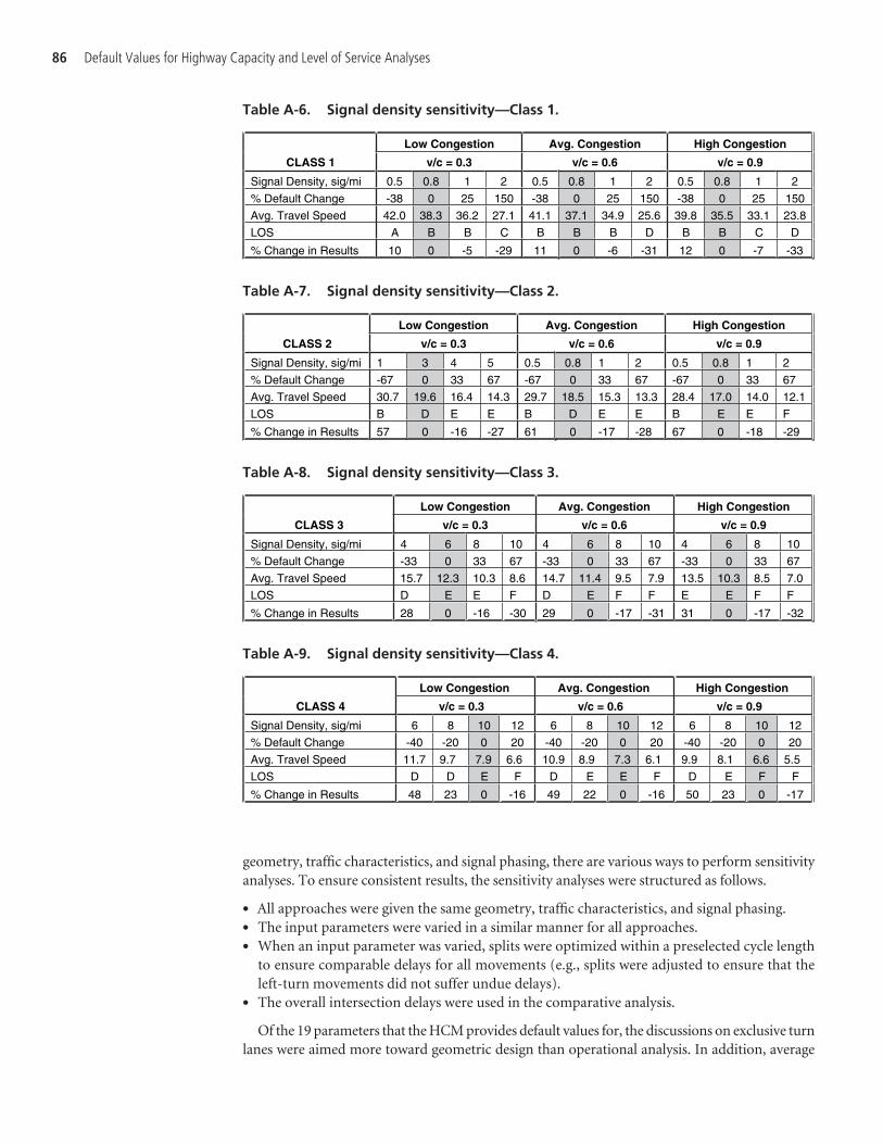
geometry, traffic characteristics, and signal phasing, there are various ways to perform sensitivityanalyses. To ensure consistent results, the sensitivity analyses were structured as follows.
• All approaches were given the same geometry, traffic characteristics, and signal phasing.• The input parameters were varied in a similar manner for all approaches.• When an input parameter was varied, splits were optimized within a preselected cycle length
to ensure comparable delays for all movements (e.g., splits were adjusted to ensure that theleft-turn movements did not suffer undue delays).
• The overall intersection delays were used in the comparative analysis.
Of the 19 parameters that the HCM provides default values for, the discussions on exclusive turnlanes were aimed more toward geometric design than operational analysis. In addition, average
86 Default Values for Highway Capacity and Level of Service Analyses
Low Congestion Avg. Congestion High Congestion
CLASS 1 v/c = 0.3 v/c = 0.6 v/c = 0.9
Signal Density, sig/mi 0.5 0.8 1 2 0.5 0.8 1 2 0.5 0.8 1 2
% Default Change -38 0 25 150 -38 0 25 150 -38 0 25 150
Avg. Travel Speed 42.0 38.3 36.2 27.1 41.1 37.1 34.9 25.6 39.8 35.5 33.1 23.8
LOS A B B C B B B D B B C D
% Change in Results 10 0 -5 -29 11 0 -6 -31 12 0 -7 -33
Table A-6. Signal density sensitivity—Class 1.
Low Congestion Avg. Congestion High Congestion
CLASS 2 v/c = 0.3 v/c = 0.6 v/c = 0.9
Signal Density, sig/mi 1 3 4 5 0.5 0.8 1 2 0.5 0.8 1 2
% Default Change -67 0 33 67 -67 0 33 67 -67 0 33 67
Avg. Travel Speed 30.7 19.6 16.4 14.3 29.7 18.5 15.3 13.3 28.4 17.0 14.0 12.1
LOS B D E E B D E E B E E F
% Change in Results 57 0 -16 -27 61 0 -17 -28 67 0 -18 -29
Low Congestion Avg. Congestion High Congestion
CLASS 3 v/c = 0.3 v/c = 0.6 v/c = 0.9
Signal Density, sig/mi 4 6 8 10 4 6 8 10 4 6 8 10
% Default Change -33 0 33 67 -33 0 33 67 -33 0 33 67
Avg. Travel Speed 15.7 12.3 10.3 8.6 14.7 11.4 9.5 7.9 13.5 10.3 8.5 7.0
LOS D E E F D E F F E E F F
% Change in Results 28 0 -16 -30 29 0 -17 -31 31 0 -17 -32
Table A-7. Signal density sensitivity—Class 2.
Table A-8. Signal density sensitivity—Class 3.
Low Congestion Avg. Congestion High Congestion
CLASS 4 v/c = 0.3 v/c = 0.6 v/c = 0.9
Signal Density, sig/mi 6 8 10 12 6 8 10 12 6 8 10 12
% Default Change -40 -20 0 20 -40 -20 0 20 -40 -20 0 20
Avg. Travel Speed 11.7 9.7 7.9 6.6 10.9 8.9 7.3 6.1 9.9 8.1 6.6 5.5
LOS D D E F D E E F D E F F
% Change in Results 48 23 0 -16 49 22 0 -16 50 23 0 -17
Table A-9. Signal density sensitivity—Class 4.
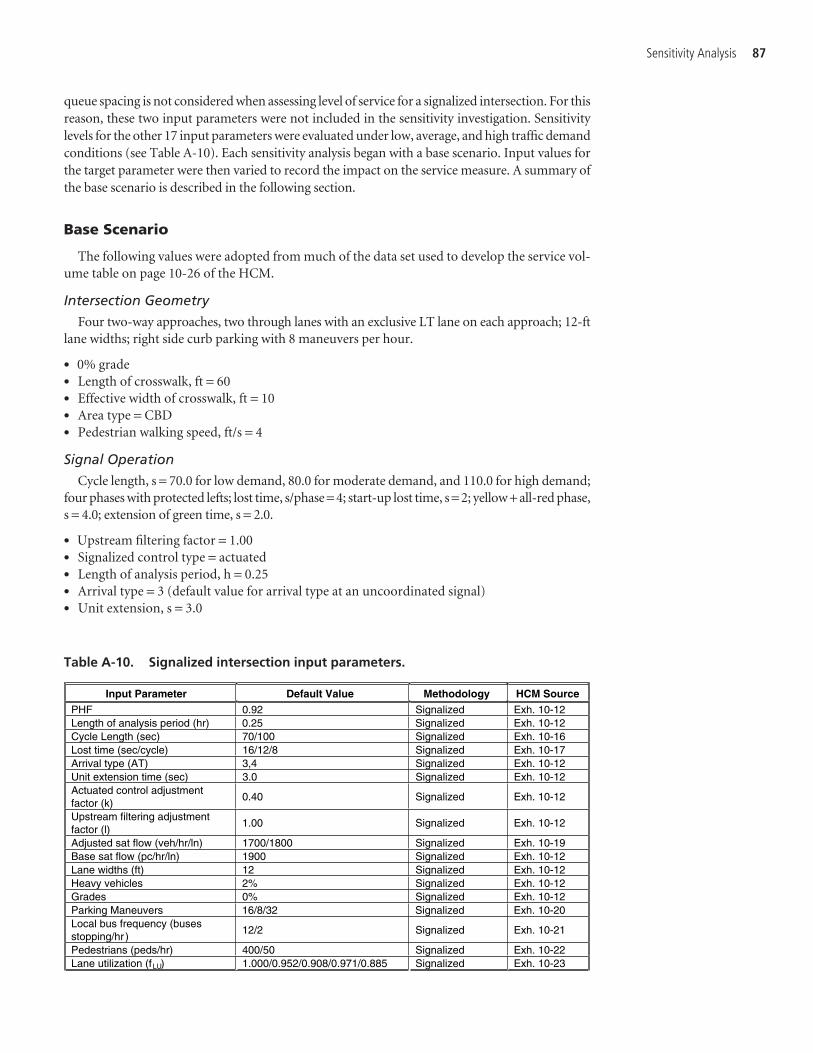
Sensitivity Analysis 87
queue spacing is not considered when assessing level of service for a signalized intersection. For thisreason, these two input parameters were not included in the sensitivity investigation. Sensitivitylevels for the other 17 input parameters were evaluated under low, average, and high traffic demandconditions (see Table A-10). Each sensitivity analysis began with a base scenario. Input values forthe target parameter were then varied to record the impact on the service measure. A summary ofthe base scenario is described in the following section.
Base Scenario
The following values were adopted from much of the data set used to develop the service vol-ume table on page 10-26 of the HCM.
Intersection Geometry
Four two-way approaches, two through lanes with an exclusive LT lane on each approach; 12-ftlane widths; right side curb parking with 8 maneuvers per hour.
• 0% grade• Length of crosswalk, ft = 60• Effective width of crosswalk, ft = 10• Area type = CBD• Pedestrian walking speed, ft/s = 4
Signal Operation
Cycle length, s = 70.0 for low demand, 80.0 for moderate demand, and 110.0 for high demand;four phases with protected lefts; lost time, s/phase = 4; start-up lost time, s = 2; yellow + all-red phase,s = 4.0; extension of green time, s = 2.0.
• Upstream filtering factor = 1.00• Signalized control type = actuated• Length of analysis period, h = 0.25• Arrival type = 3 (default value for arrival type at an uncoordinated signal)• Unit extension, s = 3.0
Input Parameter Default Value Methodology HCM Source PHF 0.92 Signalized Exh. 10-12 Length of analysis period (hr) 0.25 Signalized Exh. 10-12 Cycle Length (sec) 70/100 Signalized Exh. 10-16 Lost time (sec/cycle) 16/12/8 Signalized Exh. 10-17 Arrival type (AT) 3,4 Signalized Exh. 10-12 Unit extension time (sec) 3.0 Signalized Exh. 10-12 Actuated control adjustment factor (k)
0.40 Signalized Exh. 10-12
Upstream filtering adjustment factor (l)
1.00 Signalized Exh. 10-12
Adjusted sat flow (veh/hr/ln) 1700/1800 Signalized Exh. 10-19 Base sat flow (pc/hr/ln) 1900 Signalized Exh. 10-12 Lane widths (ft) 12 Signalized Exh. 10-12 Heavy vehicles 2% Signalized Exh. 10-12 Grades 0% Signalized Exh. 10-12 Parking Maneuvers 16/8/32 Signalized Exh. 10-20 Local bus frequency (buses stopping/hr )
12/2 Signalized Exh. 10-21
Pedestrians (peds/hr) 400/50 Signalized Exh. 10-22 Lane utilization (fLU) 1.000/0.952/0.908/0.971/0.885 Signalized Exh. 10-23
Table A-10. Signalized intersection input parameters.
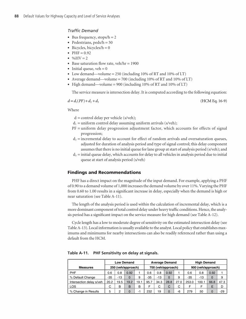
Traffic Demand
• Bus frequency, stops/h = 2• Pedestrians, peds/h = 50• Bicycles, bicycles/h = 0• PHF = 0.92• %HV = 2• Base saturation flow rate, veh/hr = 1900• Initial queue, veh = 0• Low demand—volume = 250 (including 10% of RT and 10% of LT)• Average demand—volume = 700 (including 10% of RT and 10% of LT)• High demand—volume = 900 (including 10% of RT and 10% of LT)
The service measure is intersection delay. It is computed according to the following equation:
Where
d = control delay per vehicle (s/veh);d1 = uniform control delay assuming uniform arrivals (s/veh);
PF = uniform delay progression adjustment factor, which accounts for effects of signal progression;
d2 = incremental delay to account for effect of random arrivals and oversaturation queues,adjusted for duration of analysis period and type of signal control; this delay componentassumes that there is no initial queue for lane group at start of analysis period (s/veh); and
d3 = initial queue delay, which accounts for delay to all vehicles in analysis period due to initialqueue at start of analysis period (s/veh)
Findings and Recommendations
PHF has a direct impact on the magnitude of the input demand. For example, applying a PHFof 0.90 to a demand volume of 1,000 increases the demand volume by over 11%. Varying the PHFfrom 0.60 to 1.00 results in a significant increase in delay, especially when the demand is high ornear saturation (see Table A-11).
The length of the analysis period is used within the calculation of incremental delay, which is amore dominant component of total control delay under heavy traffic conditions. Hence, the analy-sis period has a significant impact on the service measure for high demand (see Table A-12).
Cycle length has a low to moderate degree of sensitivity on the estimated intersection delay (seeTable A-13). Local information is usually available to the analyst. Local policy that establishes max-imums and minimums for nearby intersections can also be readily referenced rather than using adefault from the HCM.
d d PF d d= + +1 2 3( ) (HCM Eq. 16-9)
88 Default Values for Highway Capacity and Level of Service Analyses
Low Demand Average Demand High Demand
Measures 250 (veh/approach) 700 (veh/approach) 900 (veh/approach)
PHF 0.6 0.8 0.92 1 0.6 0.8 0.92 1 0.6 0.8 0.92 1
% Default Change -35 -13 0 9 -35 -13 0 9 -35 -13 0 9
Intersection delay s/veh 20.2 19.5 19.2 19.1 95.7 34.3 28.8 27.0 253.0 100.1 66.8 47.3
LOS C B B B F C C C F F E D
% Change in Results 5 2 0 -1 232 19 0 -6 279 50 0 -29
Table A-11. PHF Sensitivity on delay at signals.
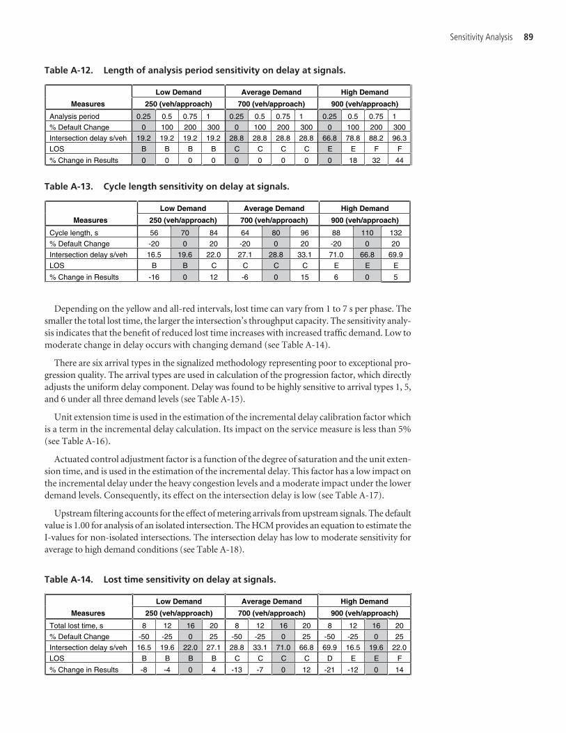
Sensitivity Analysis 89
Depending on the yellow and all-red intervals, lost time can vary from 1 to 7 s per phase. Thesmaller the total lost time, the larger the intersection’s throughput capacity. The sensitivity analy-sis indicates that the benefit of reduced lost time increases with increased traffic demand. Low tomoderate change in delay occurs with changing demand (see Table A-14).
There are six arrival types in the signalized methodology representing poor to exceptional pro-gression quality. The arrival types are used in calculation of the progression factor, which directlyadjusts the uniform delay component. Delay was found to be highly sensitive to arrival types 1, 5,and 6 under all three demand levels (see Table A-15).
Unit extension time is used in the estimation of the incremental delay calibration factor whichis a term in the incremental delay calculation. Its impact on the service measure is less than 5%(see Table A-16).
Actuated control adjustment factor is a function of the degree of saturation and the unit exten-sion time, and is used in the estimation of the incremental delay. This factor has a low impact onthe incremental delay under the heavy congestion levels and a moderate impact under the lowerdemand levels. Consequently, its effect on the intersection delay is low (see Table A-17).
Upstream filtering accounts for the effect of metering arrivals from upstream signals. The defaultvalue is 1.00 for analysis of an isolated intersection. The HCM provides an equation to estimate theI-values for non-isolated intersections. The intersection delay has low to moderate sensitivity foraverage to high demand conditions (see Table A-18).
Low Demand Average Demand High Demand
Measures 250 (veh/approach) 700 (veh/approach) 900 (veh/approach)
Analysis period 0.25 0.5 0.75 1 0.25 0.5 0.75 1 0.25 0.5 0.75 1
% Default Change 0 100 200 300 0 100 200 300 0 100 200 300
Intersection delay s/veh 19.2 19.2 19.2 19.2 28.8 28.8 28.8 28.8 66.8 78.8 88.2 96.3
LOS B B B B C C C C E E F F
% Change in Results 0 0 0 0 0 0 0 0 0 18 32 44
Table A-12. Length of analysis period sensitivity on delay at signals.
Low Demand Average Demand High Demand
Measures 250 (veh/approach) 700 (veh/approach) 900 (veh/approach)
Cycle length, s 56 70 84 64 80 96 88 110 132
% Default Change -20 0 20 -20 0 20 -20 0 20
Intersection delay s/veh 16.5 19.6 22.0 27.1 28.8 33.1 71.0 66.8 69.9
LOS B B C C C C E E E
% Change in Results -16 0 12 -6 0 15 6 0 5
Table A-13. Cycle length sensitivity on delay at signals.
Low Demand Average Demand High Demand
Measures 250 (veh/approach) 700 (veh/approach) 900 (veh/approach)
Total lost time, s 8 12 16 20 8 12 16 20 8 12 16 20
% Default Change -50 -25 0 25 -50 -25 0 25 -50 -25 0 25
Intersection delay s/veh 16.5 19.6 22.0 27.1 28.8 33.1 71.0 66.8 69.9 16.5 19.6 22.0
LOS B B B B C C C C D E E F
% Change in Results -8 -4 0 4 -13 -7 0 12 -21 -12 0 14
Table A-14. Lost time sensitivity on delay at signals.
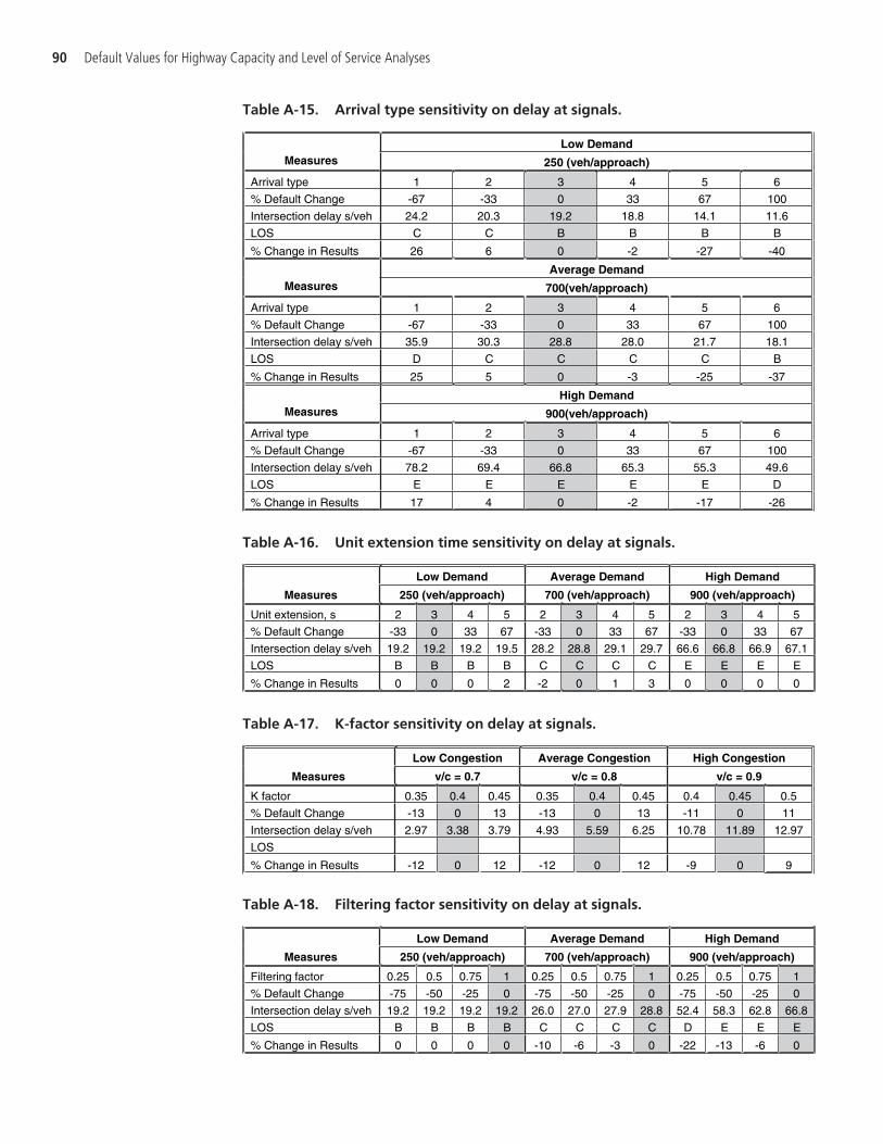
90 Default Values for Highway Capacity and Level of Service Analyses
Low DemandMeasures 250 (veh/approach)
Arrival type 1 2 3 4 5 6
% Default Change -67 -33 0 33 67 100
Intersection delay s/veh 24.2 20.3 19.2 18.8 14.1 11.6
LOS C C B B B B
% Change in Results 26 6 0 -2 -27 -40
Average DemandMeasures 700(veh/approach)
Arrival type 1 2 3 4 5 6
% Default Change -67 -33 0 33 67 100
Intersection delay s/veh 35.9 30.3 28.8 28.0 21.7 18.1
LOS D C C C C B
% Change in Results 25 5 0 -3 -25 -37
High Demand Measures 900(veh/approach)
Arrival type 1 2 3 4 5 6
% Default Change -67 -33 0 33 67 100
Intersection delay s/veh 78.2 69.4 66.8 65.3 55.3 49.6
LOS E E E E E D
% Change in Results 17 4 0 -2 -17 -26
Low Demand Average Demand High Demand
Measures 250 (veh/approach) 700 (veh/approach) 900 (veh/approach)
Unit extension, s 2 3 4 5 2 3 4 5 2 3 4 5
% Default Change -33 0 33 67 -33 0 33 67 -33 0 33 67
Intersection delay s/veh 19.2 19.2 19.2 19.5 28.2 28.8 29.1 29.7 66.6 66.8 66.9 67.1
LOS B B B B C C C C E E E E
% Change in Results 0 0 0 2 -2 0 1 3 0 0 0 0
Table A-15. Arrival type sensitivity on delay at signals.
Table A-16. Unit extension time sensitivity on delay at signals.
Low Congestion Average Congestion High Congestion
Measures v/c = 0.7 v/c = 0.8 v/c = 0.9
K factor 0.35 0.4 0.45 0.35 0.4 0.45 0.4 0.45 0.5
% Default Change -13 0 13 -13 0 13 -11 0 11
Intersection delay s/veh 2.97 3.38 3.79 4.93 5.59 6.25 10.78 11.89 12.97
LOS
% Change in Results -12 0 12 -12 0 12 -9 0 9
Table A-17. K-factor sensitivity on delay at signals.
Low Demand Average Demand High Demand
Measures 250 (veh/approach) 700 (veh/approach) 900 (veh/approach)
Filtering factor 0.25 0.5 0.75 1 0.25 0.5 0.75 1 0.25 0.5 0.75 1
% Default Change -75 -50 -25 0 -75 -50 -25 0 -75 -50 -25 0
Intersection delay s/veh 19.2 19.2 19.2 19.2 26.0 27.0 27.9 28.8 52.4 58.3 62.8 66.8
LOS B B B B C C C C D E E E
% Change in Results 0 0 0 0 -10 -6 -3 0 -22 -13 -6 0
Table A-18. Filtering factor sensitivity on delay at signals.

Sensitivity Analysis 91
The signalized method allows the user to override the estimated adjusted saturation flow ratewith field measured values. The saturation flow rate parameter has a low degree of sensitivityunder low and average traffic conditions and a significant degree of sensitivity when trafficdemand approaches or exceeds saturation (see Table A-19). At oversaturation levels, the satu-ration flow rate should not be defaulted. If field-measured values are not available, it should beestimated from the base saturation flow rate and adjustment factors as detailed in the HCM.
When base saturation flow rate cannot be measured in the field, a default value is used. A defaultvalue of 1,900 is often used in analyses. The sensitivity results indicate that this input parameter hasa low impact on delay under low demand, a moderate impact at average demand, and a significantimpact under congested conditions (see Table A-20).
The base saturation flow rate is adjusted by the lane width, %HV, percent grade, bus, pedes-trian, and parking movements, and lane utilization. A decrease in the lane width decreases the sat-uration flow and results in a similar sensitivity to that illustrated for the base saturation flow (seeTable A-21).
Increasing %HV results in a decrease in the saturation flow rate. Fifteen %HV was found toincrease the delay by as much as 60% under high demand conditions (see Table A-22). Thisparameter has a much more significant effect on the signal operation than other facilities types.
According to its adjustment equation, every 1% in approach grade results in a 0.5% reduc-tion in saturation flow rate, which consequently results in a low to moderate impact on the delay(see Table A-23).
Low Demand Average Demand High Demand
Measure 250 (veh/approach) 700 (veh/approach) 900 (veh/approach)
Adjusted sat. flow, pc/h 1500 1600 1700 1800 1500 1600 1700 1800 1500 1600 1700 1800
% Default Change -12 -6 0 6 -12 -6 0 6 -12 -6 0 6
Intersection delay s/veh 19.2 19.1 19.0 19.0 28.0 26.9 26.2 25.6 58.3 48.3 43.4 40.5
LOS B B B B C C C C E D D D
% Change in Results 1 1 0 0 7 3 0 -2 34 11 0 -7
Table A-19. Adjusted saturation flow sensitivity on delay at signals.
Low Demand Average Demand High Demand
Measures 250 (veh/approach) 700 (veh/approach) 900 (veh/approach)
Base Sat flow, pc/h 1700 1800 1900 2000 1700 1800 1900 2000 1700 1800 1900 2000
% Default Change -11 -5 0 5 -11 -5 0 5 -11 -5 0 5
Intersection delay s/veh 19.4 19.3 19.2 19.2 32.6 26.9 28.8 27.7 103.0 82.2 66.8 55.3
LOS B B B B C C C C F F E E
% Change in Results 1 1 0 0 13 -7 0 -4 54 23 0 -17
Table A-20. Base saturation flow sensitivity on delay at signals.
Low Demand Average Demand High Demand
Measures 250 (veh/approach) 700 (veh/approach) 900 (veh/approach)
Lane width, ft 9 10 12 14 9 10 12 14 9 10 12 14
% Default Change -25 -17 0 17 -25 -17 0 17 -25 -17 0 17
Intersection delay s/veh 19.4 19.4 19.2 19.2 33.1 31.3 28.8 27.1 102.3 88.1 66.8 52.5
LOS B B B B C C C C F F E D
% Change in Results 1 1 0 0 15 9 0 -6 53 32 0 -21
Table A-21. Lane width sensitivity on delay at signals.
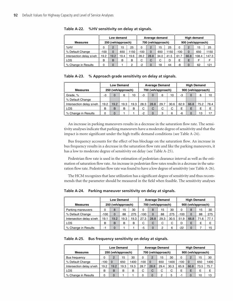
An increase in parking maneuvers results in a decrease in the saturation flow rate. The sensi-tivity analyses indicate that parking maneuvers have a moderate degree of sensitivity and that theimpact is more significant under the high traffic demand conditions (see Table A-24).
Bus frequency accounts for the effect of bus blockage on the saturation flow. An increase inbus frequency results in a decrease in the saturation flow rate and like the parking maneuvers, ithas a low to moderate degree of sensitivity on delay (see Table A-25).
Pedestrian flow rate is used in the estimation of pedestrian clearance interval as well as the esti-mation of saturation flow rate. An increase in pedestrian flow rates results in a decrease in the satu-ration flow rate. Pedestrian flow rate was found to have a low degree of sensitivity (see Table A-26).
The HCM recognizes that lane utilization has a significant degree of sensitivity and thus recom-mends that the parameter should be measured in the field when feasible. The sensitivity analyses
92 Default Values for Highway Capacity and Level of Service Analyses
Low demand Average demand High demand
Measures 250 (veh/approach) 700 (veh/approach) 900 (veh/approach)
%HV 0 2 15 25 0 2 15 25 0 2 15 25
% Default Change -100 0 650 1150 -100 0 650 1150 -100 0 650 1150
Intersection delay s/veh 19.2 19.2 19.4 19.6 28.2 28.8 34.0 41.5 61.7 66.8 108.4 147.3
LOS B B B B C C C D E E F F
% Change in Results 0 0 1 2 -2 0 18 44 -8 0 62 121
Table A-22. %HV sensitivity on delay at signals.
Low Demand Average Demand High Demand
Measures 250 (veh/approach) 700 (veh/approach) 900 (veh/approach)
Grade, % -3 0 6 10 -3 0 6 10 -3 0 6 10
% Default Change
Intersection delay s/veh 19.2 19.2 19.3 19.3 28.3 28.8 29.7 30.6 62.9 66.8 75.2 78.4
LOS B B B B C C C C E E E E
% Change in Results 0 0 1 1 -2 0 3 6 -6 0 13 17
Measures
Parking maneuvers 0 8 15 30 0 8 15 30 0 8 15 30
% Default Change -100 0 88 275 -100 0 88 275 -100 0 88 275
Intersection delay s/veh 19.1 19.2 19.3 19.3 27.3 28.8 29.3 30.5 51.9 66.8 71.6 77.1
LOS B B B B C C C C D E E E
% Change in Results -1 0 1 1 -5 0 2 6 -22 0 7 15
Low Demand Average Demand High Demand
250 (veh/approach) 700 (veh/approach) 900 (veh/approach)
Table A-23. % Approach grade sensitivity on delay at signals.
Table A-24. Parking maneuver sensitivity on delay at signals.
Measures
Bus frequency 0 2 15 30 0 2 15 30 0 2 15 30
% Default Change -100 0 650 1400 -100 0 650 1400 -100 0 650 1400
Intersection delay s/veh 19.2 19.2 19.3 19.3 28.7 28.8 29.4 30.3 65.9 66.8 73.5 75.7
LOS B B B B C C C C E E E E
% Change in Results 0 0 1 1 0 0 2 5 -1 0 10 13
Low Demand
250 (veh/approach)
Average Demand
700 (veh/approach)
High Demand
900 (veh/approach)
Table A-25. Bus frequency sensitivity on delay at signals.
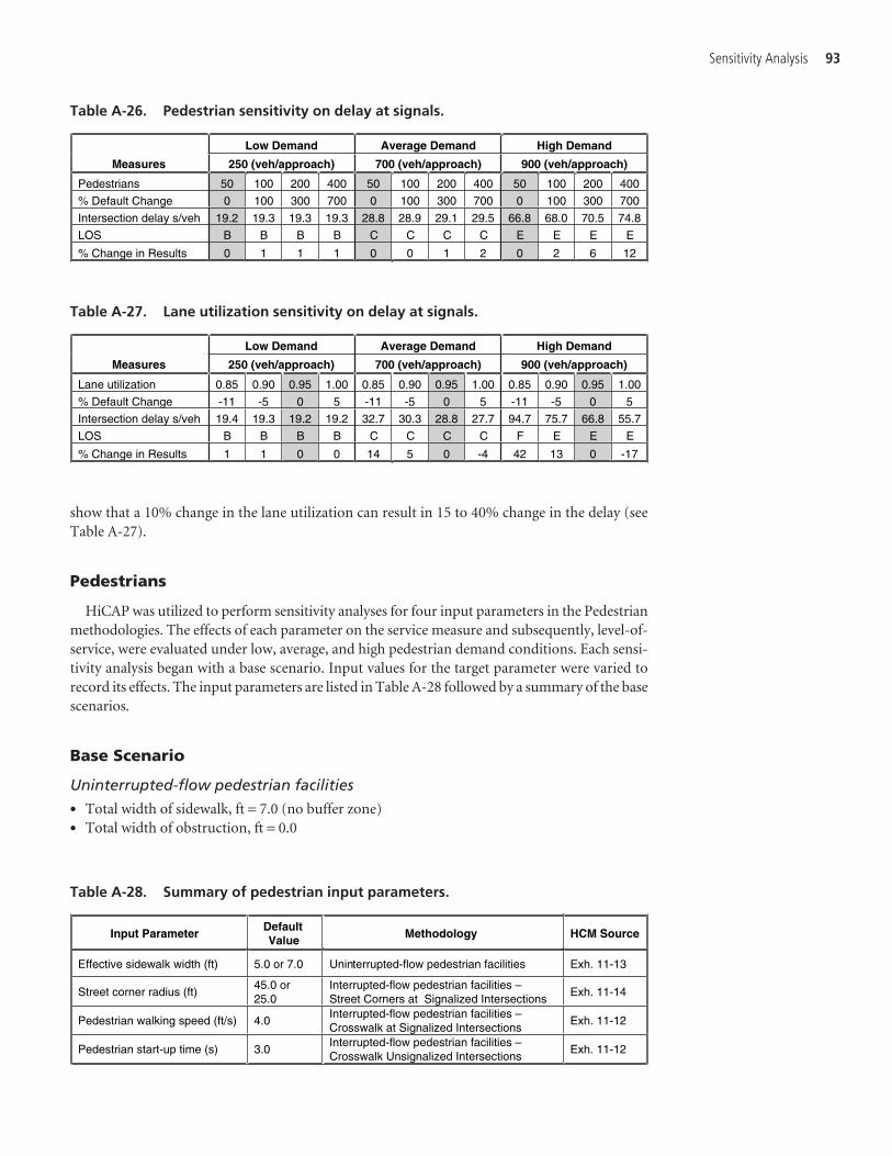
Sensitivity Analysis 93
show that a 10% change in the lane utilization can result in 15 to 40% change in the delay (seeTable A-27).
Pedestrians
HiCAP was utilized to perform sensitivity analyses for four input parameters in the Pedestrianmethodologies. The effects of each parameter on the service measure and subsequently, level-of-service, were evaluated under low, average, and high pedestrian demand conditions. Each sensi-tivity analysis began with a base scenario. Input values for the target parameter were varied torecord its effects. The input parameters are listed in Table A-28 followed by a summary of the basescenarios.
Base Scenario
Uninterrupted-flow pedestrian facilities
• Total width of sidewalk, ft = 7.0 (no buffer zone)• Total width of obstruction, ft = 0.0
Measures
Pedestrians 50 100 200 400 50 100 200 400 50 100 200 400
% Default Change 0 100 300 700 0 100 300 700 0 100 300 700
Intersection delay s/veh 19.2 19.3 19.3 19.3 28.8 28.9 29.1 29.5 66.8 68.0 70.5 74.8
LOS B B B B C C C C E E E E
% Change in Results 0 1 1 1 0 0 1 2 0 2 6 12
Low Demand
250 (veh/approach)
Average Demand
700 (veh/approach)
High Demand
900 (veh/approach)
Table A-26. Pedestrian sensitivity on delay at signals.
Measures
Lane utilization 0.85 0.90 0.95 1.00 0.85 0.90 0.95 1.00 0.85 0.90 0.95 1.00
% Default Change -11 -5 0 5 -11 -5 0 5 -11 -5 0 5
Intersection delay s/veh 19.4 19.3 19.2 19.2 32.7 30.3 28.8 27.7 94.7 75.7 66.8 55.7
LOS B B B B C C C C F E E E
% Change in Results 1 1 0 0 14 5 0 -4 42 13 0 -17
Low Demand
250 (veh/approach)
Average Demand
700 (veh/approach)
High Demand
900 (veh/approach)
Table A-27. Lane utilization sensitivity on delay at signals.
Input Parameter DefaultValue
Methodology HCM Source
Effective sidewalk width (ft) 5.0 or 7.0 Uninterrupted-flow pedestrian facilities Exh. 11-13
Street corner radius (ft) 45.0 or 25.0
Interrupted-flow pedestrian facilities – Street Corners at Signalized Intersections
Exh. 11-14
Pedestrian walking speed (ft/s) 4.0 Interrupted-flow pedestrian facilities – Crosswalk at Signalized Intersections
Exh. 11-12
Pedestrian start-up time (s) 3.0 Interrupted-flow pedestrian facilities – Crosswalk Unsignalized Intersections
Exh. 11-12
Table A-28. Summary of pedestrian input parameters.
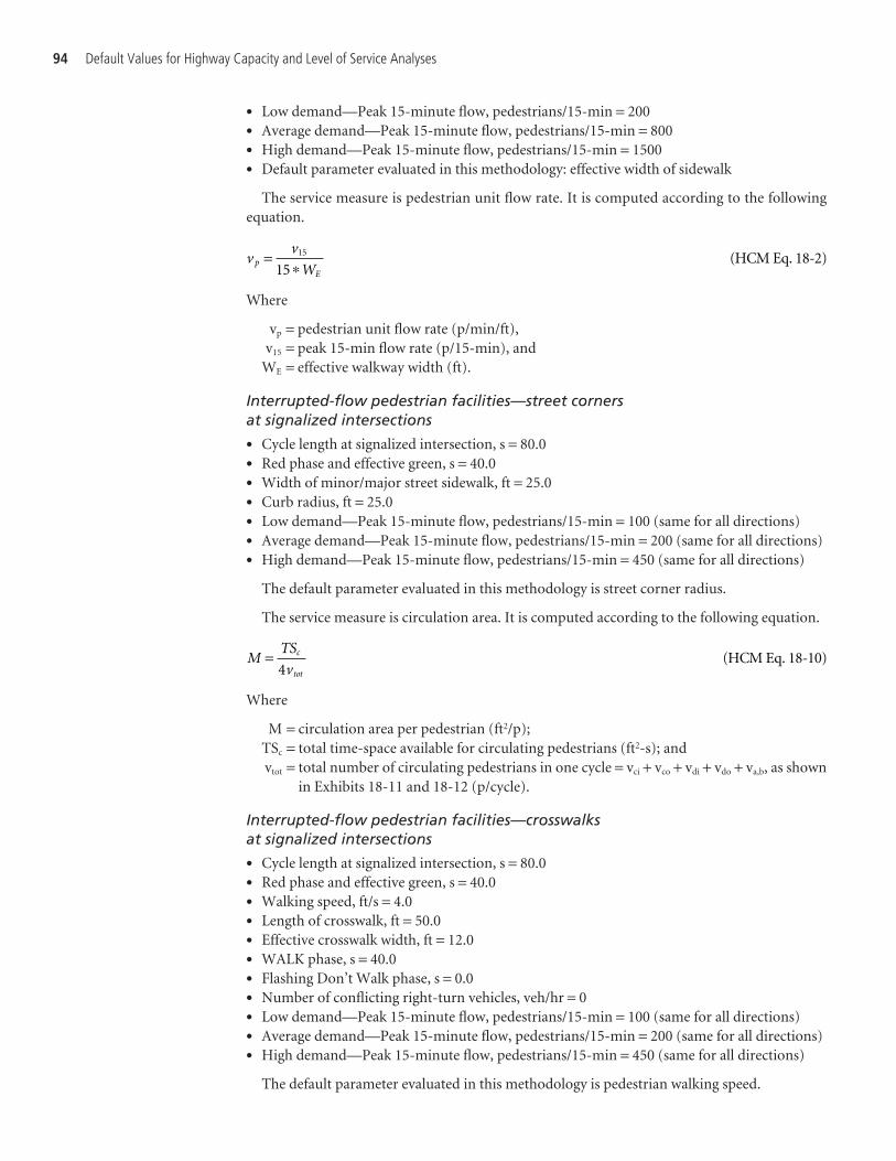
• Low demand—Peak 15-minute flow, pedestrians/15-min = 200• Average demand—Peak 15-minute flow, pedestrians/15-min = 800• High demand—Peak 15-minute flow, pedestrians/15-min = 1500• Default parameter evaluated in this methodology: effective width of sidewalk
The service measure is pedestrian unit flow rate. It is computed according to the followingequation.
Where
vp = pedestrian unit flow rate (p/min/ft),v15 = peak 15-min flow rate (p/15-min), and
WE = effective walkway width (ft).
Interrupted-flow pedestrian facilities—street corners at signalized intersections
• Cycle length at signalized intersection, s = 80.0• Red phase and effective green, s = 40.0• Width of minor/major street sidewalk, ft = 25.0• Curb radius, ft = 25.0• Low demand—Peak 15-minute flow, pedestrians/15-min = 100 (same for all directions)• Average demand—Peak 15-minute flow, pedestrians/15-min = 200 (same for all directions)• High demand—Peak 15-minute flow, pedestrians/15-min = 450 (same for all directions)
The default parameter evaluated in this methodology is street corner radius.
The service measure is circulation area. It is computed according to the following equation.
Where
M = circulation area per pedestrian (ft2/p);TSc = total time-space available for circulating pedestrians (ft2-s); andvtot = total number of circulating pedestrians in one cycle = vci + vco + vdi + vdo + va,b, as shown
in Exhibits 18-11 and 18-12 (p/cycle).
Interrupted-flow pedestrian facilities—crosswalks at signalized intersections
• Cycle length at signalized intersection, s = 80.0• Red phase and effective green, s = 40.0• Walking speed, ft/s = 4.0• Length of crosswalk, ft = 50.0• Effective crosswalk width, ft = 12.0• WALK phase, s = 40.0• Flashing Don’t Walk phase, s = 0.0• Number of conflicting right-turn vehicles, veh/hr = 0• Low demand—Peak 15-minute flow, pedestrians/15-min = 100 (same for all directions)• Average demand—Peak 15-minute flow, pedestrians/15-min = 200 (same for all directions)• High demand—Peak 15-minute flow, pedestrians/15-min = 450 (same for all directions)
The default parameter evaluated in this methodology is pedestrian walking speed.
MTS
vc
tot
=4
(HCM Eq. 18-10)
vv
Wp
E
= 15
15 �(HCM Eq. 18-2)
94 Default Values for Highway Capacity and Level of Service Analyses

Sensitivity Analysis 95
The service measure is circulation area. It is computed according to the following equation.
Where
M = circulation area per pedestrian (ft2/p),TS = time-space (ft2-s), and
T = total crosswalk occupancy time (p-s).
Interrupted-flow pedestrian facilities—street corners at unsignalized intersections• Total width of crosswalk, ft = 12.0• Effective width of crosswalk, ft = 12.0• Pedestrian walking speed, ft/s = 4.0• Pedestrian start-up time, s = 3.0• Length of crosswalk, ft = 36.0• Conflicting vehicle flow rate, veh/hr = 500• Low demand—Peak 15-minute flow, pedestrians/15-min = 100• Average demand—Peak 15-minute flow, pedestrians/15-min = 200• High demand—Peak 15-minute flow, pedestrians/15-min = 450
The default parameter evaluated in this methodology is pedestrian start-up time.
The service measure is average pedestrian delay. It is computed according to the followingequation.
Where
dp = average pedestrian delay (s),v = vehicular flow rate (veh/s), and
tG = group critical gap from Equation 18-19 (s).
Findings and Recommendations
Effective sidewalk width at uninterrupted pedestrian facilities was found to have a significantimpact on level of service (see Table A-29). The trend is the same in all demand levels examined.
Street corner radius, which is used to assess street corners at signalized intersections, directlyaffects the computation of available time-space. An increase in the corner radius results in a reduc-tion in circulation (see Table A-30). This reduction in circulation occurs because as the larger cor-ner radius (for turning vehicles) increases, the sidewalk area at the corner decreases. The streetcorner radius input parameter has a significant degree of sensitivity at all demand levels.
dv
e vtpvtG
G= − −( )11 (HCM Eq. 18-21)
MTS
T= (HCM Eq. 18-15)
Low Demand Average Demand High Demand
Measure Volume = 200 Volume = 800 Volume = 1500
Effective Width, ft 3 5 7 10 15 3 5 7 10 15 3 5 7 10 15
% Default Change -57 -29 0 43 114 -57 -29 0 43 114 -57 -29 0 43 114
Ped Flow, p/min/ft 4.4 2.7 1.9 1.3 0.9 17.8 10.7 7.6 5.3 3.6 33.3 20 14.3 10 6.7
LOS A A A A A E D C B A F E D C B
% Change in Results 132 42 0 -32 -53 134 41 0 -30 -53 133 40 0 -30 -53
Table A-29. Effective width sensitivity on pedestrian flow at crosswalks.
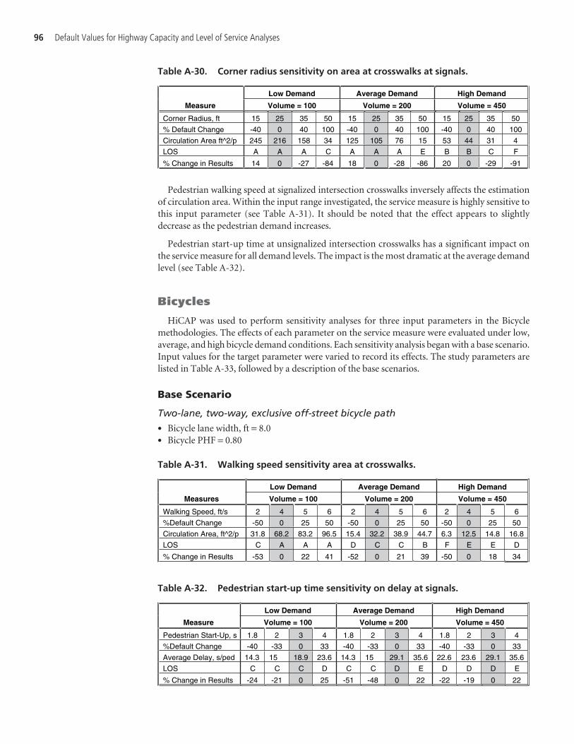
Pedestrian walking speed at signalized intersection crosswalks inversely affects the estimationof circulation area. Within the input range investigated, the service measure is highly sensitive tothis input parameter (see Table A-31). It should be noted that the effect appears to slightlydecrease as the pedestrian demand increases.
Pedestrian start-up time at unsignalized intersection crosswalks has a significant impact onthe service measure for all demand levels. The impact is the most dramatic at the average demandlevel (see Table A-32).
Bicycles
HiCAP was used to perform sensitivity analyses for three input parameters in the Bicyclemethodologies. The effects of each parameter on the service measure were evaluated under low,average, and high bicycle demand conditions. Each sensitivity analysis began with a base scenario.Input values for the target parameter were varied to record its effects. The study parameters arelisted in Table A-33, followed by a description of the base scenarios.
Base Scenario
Two-lane, two-way, exclusive off-street bicycle path• Bicycle lane width, ft = 8.0• Bicycle PHF = 0.80
96 Default Values for Highway Capacity and Level of Service Analyses
Low Demand Average Demand High Demand
Measure Volume = 100 Volume = 200 Volume = 450
Corner Radius, ft 15 25 35 50 15 25 35 50 15 25 35 50
% Default Change -40 0 40 100 -40 0 40 100 -40 0 40 100
Circulation Area ft^2/p 245 216 158 34 125 105 76 15 53 44 31 4
LOS A A A C A A A E B B C F
% Change in Results 14 0 -27 -84 18 0 -28 -86 20 0 -29 -91
Table A-30. Corner radius sensitivity on area at crosswalks at signals.
Low Demand Average Demand High Demand
Measures Volume = 100 Volume = 200 Volume = 450
Walking Speed, ft/s 2 4 5 6 2 4 5 6 2 4 5 6
%Default Change -50 0 25 50 -50 0 25 50 -50 0 25 50
Circulation Area, ft^2/p 31.8 68.2 83.2 96.5 15.4 32.2 38.9 44.7 6.3 12.5 14.8 16.8
LOS C A A A D C C B F E E D
% Change in Results -53 0 22 41 -52 0 21 39 -50 0 18 34
Table A-31. Walking speed sensitivity area at crosswalks.
Low Demand Average Demand High Demand
Measure Volume = 100 Volume = 200 Volume = 450
Pedestrian Start-Up, s 1.8 2 3 4 1.8 2 3 4 1.8 2 3 4
%Default Change -40 -33 0 33 -40 -33 0 33 -40 -33 0 33
Average Delay, s/ped 14.3 15 18.9 23.6 14.3 15 29.1 35.6 22.6 23.6 29.1 35.6
LOS C C C D C C D E D D D E
% Change in Results -24 -21 0 25 -51 -48 0 22 -22 -19 0 22
Table A-32. Pedestrian start-up time sensitivity on delay at signals.
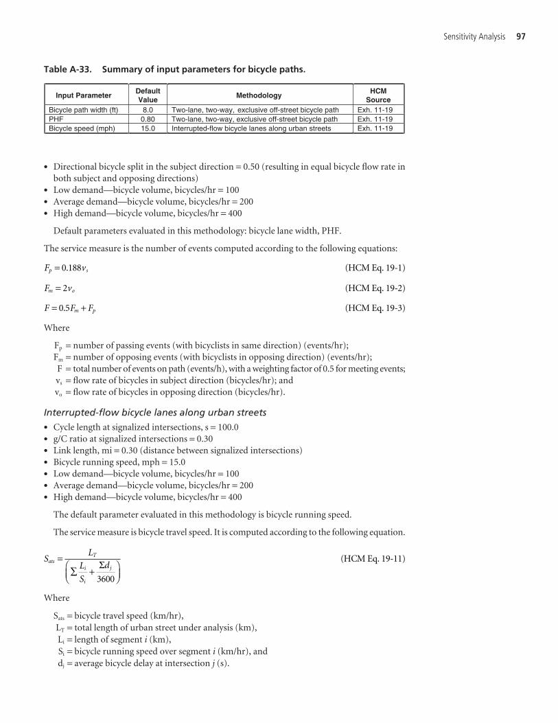
Sensitivity Analysis 97
• Directional bicycle split in the subject direction = 0.50 (resulting in equal bicycle flow rate inboth subject and opposing directions)
• Low demand—bicycle volume, bicycles/hr = 100• Average demand—bicycle volume, bicycles/hr = 200• High demand—bicycle volume, bicycles/hr = 400
Default parameters evaluated in this methodology: bicycle lane width, PHF.
The service measure is the number of events computed according to the following equations:
Where
Fp = number of passing events (with bicyclists in same direction) (events/hr);Fm = number of opposing events (with bicyclists in opposing direction) (events/hr);F = total number of events on path (events/h), with a weighting factor of 0.5 for meeting events;vs = flow rate of bicycles in subject direction (bicycles/hr); andvo = flow rate of bicycles in opposing direction (bicycles/hr).
Interrupted-flow bicycle lanes along urban streets• Cycle length at signalized intersections, s = 100.0• g/C ratio at signalized intersections = 0.30• Link length, mi = 0.30 (distance between signalized intersections)• Bicycle running speed, mph = 15.0• Low demand—bicycle volume, bicycles/hr = 100• Average demand—bicycle volume, bicycles/hr = 200• High demand—bicycle volume, bicycles/hr = 400
The default parameter evaluated in this methodology is bicycle running speed.
The service measure is bicycle travel speed. It is computed according to the following equation.
Where
Sats = bicycle travel speed (km/hr),LT = total length of urban street under analysis (km),Li = length of segment i (km),Si = bicycle running speed over segment i (km/hr), anddj = average bicycle delay at intersection j (s).
SL
L
S
dats
T
i
i
j
=∑ +
Σ⎛⎝⎜
⎞⎠⎟3600
(HCM Eq. 19-11)
F F Fm p= +0 5. (HCM Eq. 19-3)
F vm o= 2 (HCM Eq. 19-2)
F vp s= 0 188. (HCM Eq. 19-1)
Input Parameter Default Value
Methodology HC M
Source Bicycle path width (ft) 8.0 Two-lane, two-way, exclusive off-street bicycle path Exh. 11-19 PHF 0.80 Two-lane, two-way, exclusive off-street bicycle path Exh. 11-19 Bicycle speed (mph) 15.0 Interrupted-flow bicycle lanes along urban streets Exh. 11-19
Table A-33. Summary of input parameters for bicycle paths.

Findings and Recommendations
Two-lane, two-way, exclusive off-street bicycle path width does not have any impact on levelof service (see Table A-34). A closer examination of the methodologies indicates that this param-eter does not enter into the computations, and its default value of 8.0 ft was derived from theAASHTO’s Guide for Development of Bicycle Facilities.
Two-lane, two-way, exclusive off-street bicycle path PHF directly affects bicycle volume and,subsequently, level of service. The service measure has a significant sensitivity to the PHF for allthree demand levels (see Table A-35).
Interrupted-flow bicycle lane running speed along urban streets greatly affects the estimationof bicycle travel speed. Within the practical range of this parameter, the performance measurehas a significant degree of sensitivity to the running speed for all demand levels (see Table A-36).
Two-Lane Highways
In HCM 2000, two methodologies are provided to analyze a two-lane highway segment: a two-way analysis method and a directional analysis method. Because the directional analysis method
98 Default Values for Highway Capacity and Level of Service Analyses
Low Demand Measures Volume = 100
Bicycle Path Width, ft 3 5 8 10 14
% Default Change -63 -38 0 25 75
Number of Events 74 74 74 74 74
LOS C C C C C
% Change in Results 0 0 0 0 0
Average Demand Measures Volume = 200
Bicycle Path Width, ft 3 5 8 10 14
% Default Change -63 -63 -6 3 -63 -63
Number of Events 149 149 149 149 149
LOS C C C C C
% Change in Results 0 0 0 0 0
High Demand Measures Volume = 400
Bicycle Path Width, ft 3 5 8 10 14
% Default Change -63 -63 -6 3 -63 -63
Number of Events 297 297 297 297 297
LOS C C C C C
% Change in Results 0 0 0 0 0
Table A-34. Bicycle path width sensitivity on number of events.
Low Demand Average Demand High Demand
Measure Volume = 100 Volume = 200 Volume = 400
Bicycle PHF 0.6 0.8 0.9 1 0.6 0.8 0.9 1 0.6 0.8 0.9 1
% Default Change -25 0 13 25 -25 0 13 25 -25 0 13 25
Number of events 99 74 66 59 198 149 132 119 396 297 264 238
LOS C C C B F D D D F F F F
% Change in Results 34 0 -11 -20 33 0 -11 -20 33 0 -11 -20
Table A-35. PHF sensitivity on number of events at bike paths.
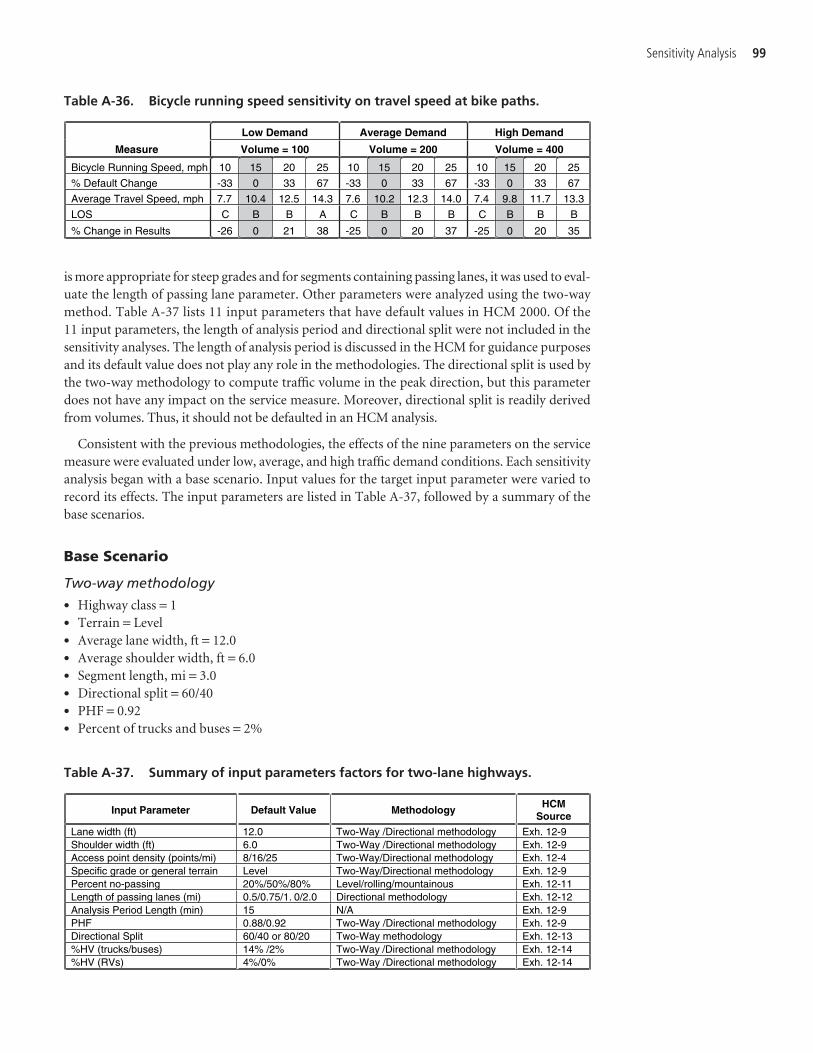
Sensitivity Analysis 99
is more appropriate for steep grades and for segments containing passing lanes, it was used to eval-uate the length of passing lane parameter. Other parameters were analyzed using the two-waymethod. Table A-37 lists 11 input parameters that have default values in HCM 2000. Of the 11 input parameters, the length of analysis period and directional split were not included in thesensitivity analyses. The length of analysis period is discussed in the HCM for guidance purposesand its default value does not play any role in the methodologies. The directional split is used bythe two-way methodology to compute traffic volume in the peak direction, but this parameterdoes not have any impact on the service measure. Moreover, directional split is readily derivedfrom volumes. Thus, it should not be defaulted in an HCM analysis.
Consistent with the previous methodologies, the effects of the nine parameters on the servicemeasure were evaluated under low, average, and high traffic demand conditions. Each sensitivityanalysis began with a base scenario. Input values for the target input parameter were varied torecord its effects. The input parameters are listed in Table A-37, followed by a summary of thebase scenarios.
Base Scenario
Two-way methodology
• Highway class = 1• Terrain = Level• Average lane width, ft = 12.0• Average shoulder width, ft = 6.0• Segment length, mi = 3.0• Directional split = 60/40• PHF = 0.92• Percent of trucks and buses = 2%
Low Demand Average Demand High Demand
Measure Volume = 100 Volume = 200 Volume = 400
Bicycle Running Speed, mph 10 15 20 25 10 15 20 25 10 15 20 25
% Default Change -33 0 33 67 -33 0 33 67 -33 0 33 67
Average Travel Speed, mph 7.7 10.4 12.5 14.3 7.6 10.2 12.3 14.0 7.4 9.8 11.7 13.3
LOS C B B A C B B B C B B B
% Change in Results -26 0 21 38 -25 0 20 37 -25 0 20 35
Table A-36. Bicycle running speed sensitivity on travel speed at bike paths.
Input Parameter Default Value Methodology HCM
Source
Lane width (ft) 12.0 Two-Way /Directional methodology Exh. 12-9 Shoulder width (ft) 6.0 Two-Way /Directional methodology Exh. 12-9 Access point density (points/mi) 8/16/25 Two-Way/Directional methodology Exh. 12-4 Specific grade or general terrain Level Two-Way/Directional methodology Exh. 12-9 Percent no-passing 20%/50%/80% Level/rolling/mountainous Exh. 12-11 Length of passing lanes (mi) 0.5/0.75/1. 0/2.0 Directional methodology Exh. 12-12 Analysis Period Length (min) 15 N/A Exh. 12-9 PHF 0.88/0.92 Two-Way /Directional methodology Exh. 12-9 Directional Split 60/40 or 80/20 Two-Way methodology Exh. 12-13 %HV (trucks/buses) 14% /2% Two-Way /Directional methodology Exh. 12-14 %HV (RVs) 4%/0% Two-Way /Directional methodology Exh. 12-14
Table A-37. Summary of input parameters factors for two-lane highways.

• Percent of recreational vehicles = 0%• Percent of no-passing zone = 20%• Access point density, points/mi = 16• Base free-flow speed, mph = 65• Low demand—two-way traffic volume, veh/hr = 500• Average demand—two-way traffic volume, veh/hr = 1,000• High demand—two-way traffic volume, veh/hr = 1,600
The input parameters evaluated in this methodology are lane width, shoulder width, accesspoint density, grade, percent of no-passing zone, length of passing lane, PHF, percent of trucksand buses, and percent of recreational vehicles.
The service measures are percent time spent following and average travel speed. They are com-puted according to the following equations.
Where
ATS = average travel speed for both directions of travel combined (mph),fnp = adjustment for percentage of no-passing zones (see Exhibit 20-11), andvp = passenger-car equivalent flow rate for peak 15-min period (pc/hr).
Where
PTSF = percent time-spent-following,BPTSF = base percent time-spent-following for both directions of travel combined (use Equa-
tion 20-7), andfd/np = adjustment for the combined effect of the directional distribution of traffic and of
the percentage of no-passing zones on percent time-spent-following.
Directional methodology
• Highway class = 1• Terrain = Level• Average lane width, ft = 12.0• Average shoulder width, ft = 6.0• Segment length, mi = 3.0• PHF = 0.92• Percent of trucks and buses = 2%• Percent of recreational vehicles = 0%• Percent of no-passing zone = 20%• Access point density, points/mi = 16• Base free-flow speed, mph = 65• Length of segment upstream of passing lane, mi = 0.3• Length of passing lane, mi = 0.5• Low demand—subject/opposing traffic volume, veh/hr = 200/133• Average demand—subject/opposing traffic volume, veh/hr = 400/267• High demand—subject/opposing traffic volume, veh/hr = 700/467
The default parameter evaluated in this methodology is the length of passing lane.
PTSF BPTSF fd np= + (HCM Eq. 20-6)
ATS FFS v fp np= – . –0 00776 (HCM Eq. 20-5)
100 Default Values for Highway Capacity and Level of Service Analyses

Sensitivity Analysis 101
The service measures are average travel speed and percent time-spent-following. They arecomputed according to the following equations.
Where
ATSd = average travel speed in the analysis direction (mph),FFSd = free-flow speed in the analysis direction (mph),
vd = passenger-car equivalent flow rate for the peak 15-min period in the analysis direction(pc/hr),
vo = passenger-car equivalent flow rate for the peak 15-min period in the opposingdirection (pc/hr), determined from Equation 20-13; and
fnp = adjustment for percentage of no-passing zones in the analysis direction (see Exhibit 20-19).
Where
PTSFd = percent time-spent-following in the direction analyzed,BPTSFd = base percent time-spent-following in the direction analyzed, and
fnp = adjustment for percentage of no-passing zones in the analysis direction (see Exhi-bit 20-20).
Findings and Recommendations
Lane width does not enter into the calculation of percent time-spent-following; therefore, it doesnot affect this service measure. It does have an impact on the travel speed, but the impact is verylow (less than 5%) in all three demand levels (see Table A-38).
Shoulder width has no impact on percent time-spent-following and a low impact on travel speed(see Table A-39).
Access point density is not used to calculate percent time-spent-following and has a low impacton travel speed. A 150% increase in access point density results in approximately 10% change inthe average travel (see Table A-40).
The two-way methodology only provides adjustment factors for level and rolling terrain. Moun-tainous terrain can be analyzed as specific grades using the directional method. The analysis resultsindicate that terrain has a low degree of sensitivity, less than 5% impact on either service measures,and becomes less sensitive as the traffic volume increases (see Table A-41).
PTSF BPTSF fd d np= + (HCM Eq. 20-16)
ATS FFS v v fd d d o np= − +( )−0 00776. (HCM Eq. 20-15)
Low Demand Average Demand High Demand
Measures 2-Way Volume = 500 2-Way Volume = 1000 2-Way Volume = 1600
Lane width, ft 9 10 11 12 9 10 11 12 9 10 11 12
% Default Change -25 -17 -8 0 -25 -17 -8 0 -25 -17 -8 0
%Time-spent Following 49.6 49.6 49.6 49.6 67.3 67.3 67.3 67.3 81.2 81.2 81.2 81.2
% Change in Results 0 0 0 0 0 0 0 0 0 0 0 0
Average Travel Speed, mph 52.9 54 54.7 55.1 49.4 50.5 51.2 51.6 44.7 45.8 46.5 46.9
% Change in Results -4 -2 -1 0 -4 -2 -1 0 -5 -2 -1 0
LOS B B B B D D D D E E E E
Table A-38. Lane width sensitivity on travel speed at two-lane highways.
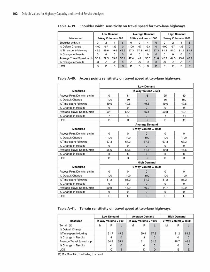
102 Default Values for Highway Capacity and Level of Service Analyses
Low Demand Average Demand High Demand
Measures 2-Way Volume = 500 2-Way Volume = 1000 2-Way Volume = 1600
Shoulder width, ft 0 2 4 6 0 2 4 6 0 2 4 6
% Default Change -100 -67 -33 0 -100 -67 -33 0 -100 -67 -33 0
% Time-spent-following 49.6 49.6 49.6 49.6 67.3 67.3 67.3 67.3 81.2 81.2 81.2 81.2
% Change in Results 0 0 0 0 0 0 0 0 0 0 0 0
Average Travel Speed, mph 50.9 52.5 53.8 55.1 47.4 49 50.3 51.6 42.7 44.3 45.6 46.9
% Change in Results -8 -5 -2 0 -8 -5 -3 0 -9 -6 -3 0
LOS B B B B D D D D E E E E
Table A-39. Shoulder width sensitivity on travel speed for two-lane highways.
Low Demand
Measures 2-Way Volume = 500
Access Point Density, pts/mi 0 8 16 25 40
% Default Change -100 -50 0 56 150
%Time-spent-following 49.6 49.6 49.6 49.6 49.6
% Change in Results 0 0 0 0 0
Average Travel Speed, mph 59.1 57.1 55.1 52.8 49.1
% Change in Results 7 4 0 -4 -11
LOS B B B B C
Average Demand
Measures 2-Way Volume = 1000
Access Point Density, pts/mi 0 0 0 0 0
% Default Change -100 -100 -100 -100 -100
%Time-spent-following 67.3 67.3 67.3 67.3 67.3
% Change in Results 0 0 0 0 0
Average Travel Speed, mph 55.6 53.6 51.6 49.3 45.6
% Change in Results 8 8 8 8 8
LOS D D D D D
High Demand
Measures 2-Way Volume = 1600
Access Point Density, pts/mi 0 0 0 0 0
% Default Change -100 -100 -100 -100 -100
%Time-spent-following 81.2 81.2 81.2 81.2 81.2
% Change in Results 0 0 0 0 0
Average Travel Speed, mph 50.9 48.9 46.9 44.7 40.9
% Change in Results 9 9 9 9 9
LOS E E E E E
Table A-40. Access points sensitivity on travel speed at two-lane highways.
Low Demand Average Demand High Demand
Measures 2-Way Volume = 500 2-Way Volume = 1000 2-Way Volume = 1600
Terrain (1) M R L M R L M R L
% Default Change
%Time-spent-following 51.7 49.6 69.4 67.3 81.2 81.2
% Change in Results 4 0 3 0 0 0
Average Travel Speed, mph 54.8 55.1 51 51.6 46.7 46.9
% Change in Results -1 0 -1 0 0 0
LOS C B D D E E
(1) M = Mountain; R = Rolling, L = Level
Table A-41. Terrain sensitivity on travel speed at two-lane highways.

Sensitivity Analysis 103
Low Demand
Measures 2-Way Volume = 500
% No-passing Zone 0 10 20 50 80
% Default Change -100 -50 0 150 300
%Time-spent-following 38.2 43.9 49.6 55.5 58.3
% Change in Results -23 -11 0 12 18
Average Travel Speed, mph 56.7 55.9 55.1 53.9 53.2
% Change in Results 3 1 0 -2 -3
LOS B B B C C
Average Demand
Measures 2-Way Volume = 1000
% No-passing Zone 0 10 20 50 80
% Default Change -100 -50 0 150 300
%Time-spent-following 61.6 64.5 67.3 70.7 72.4
% Change in Results -8 -4 0 5 8
Average Travel Speed, mph 52.5 52 51.6 50.9 50.5
% Change in Results 2 1 0 -1 -2
LOS C C D D D
High Demand
Measures 2-Way Volume = 1600
% No-passing Zone 0 10 20 50 80
% Default Change -100 -50 0 150 300
%Time-spent-following 78.3 79.8 81.2 83 83.9
% Change in Results -4 -2 0 2 3
Average Travel Speed, mph 47.5 47.2 46.9 46.6 46.3
% Change in Results 1 1 0 -1 -1
LOS D D E E E
Table A-42. Percent no-passing sensitivity on travel speed at two-lane highways.
Low Demand Average Demand High Demand
Measure 2-Way Volume = 500 2-Way Volume = 1000 2-Way Volume = 1600
PHF 0.6 0.88 0.92 1 0.6 0.88 0.92 1 0.6 0.88 0.92 1
% Default Change -35 -4 0 9 -35 -4 0 9 -35 -4 0 9
%Time-spent-following 59.4 50.9 49.6 47.2 80.0 68.6 67.3 64.8 91.3 82.5 81.2 78.7
% Change in Results 20 3 0 -5 19 2 0 -4 12 2 0 -3
Average Travel Speed, mph 53.2 54.9 55.1 55.4 47.5 51.3 51.6 52.1 39.8 46.4 46.9 48
% Change in Results -3 0 0 1 -8 -1 0 1 -15 -1 0 2
LOS C C B B D D D C E E E D
Table A-43. PHF sensitivity on travel speed at two-lane highways.
The percent of no-passing zone directly affects the passing opportunity. This parameter has asignificant impact on the percent time-spent-following service measure. However, the impactbecomes less significant as the traffic demand increases. It has a low effect on the average travelspeed (see Table A-42).
PHF directly adjusts the input volume and thus has a noticeable effect on the service measures(see Table A-43). It is interesting to note that the percent time-spent-following is more sensitiveto this factor under the low demand conditions and less so under the heavier demand conditions.The opposite trend is observed for the travel speed. The computed speed varies by less than 5%under the low-demand conditions but up to 15% under high-demand conditions.
Percent of trucks and buses has a low degree of sensitivity, with less than 5% impact at alldemand levels (see Table A-44).
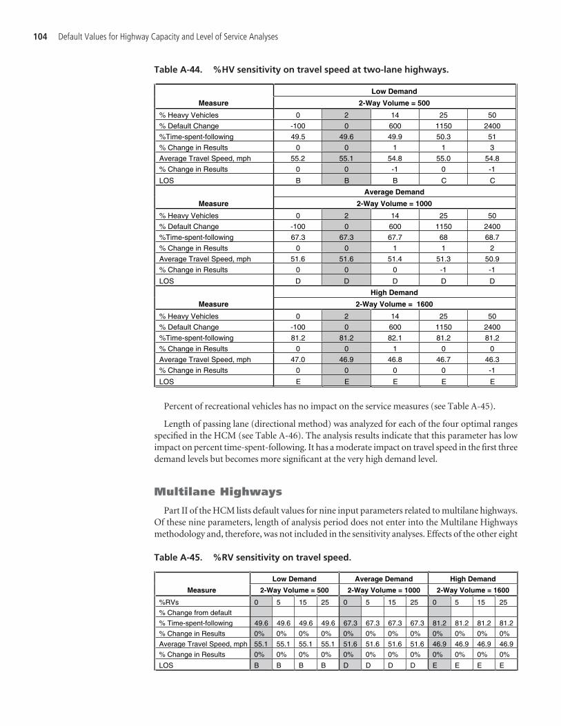
Percent of recreational vehicles has no impact on the service measures (see Table A-45).
Length of passing lane (directional method) was analyzed for each of the four optimal rangesspecified in the HCM (see Table A-46). The analysis results indicate that this parameter has lowimpact on percent time-spent-following. It has a moderate impact on travel speed in the first threedemand levels but becomes more significant at the very high demand level.
Multilane Highways
Part II of the HCM lists default values for nine input parameters related to multilane highways.Of these nine parameters, length of analysis period does not enter into the Multilane Highwaysmethodology and, therefore, was not included in the sensitivity analyses. Effects of the other eight
104 Default Values for Highway Capacity and Level of Service Analyses
Low Demand
Measure 2-Way Volume = 500
% Heavy Vehicles 0 2 14 25 50
% Default Change -100 0 600 1150 2400
%Time-spent-following 49.5 49.6 49.9 50.3 51
% Change in Results 0 0 1 1 3
Average Travel Speed, mph 55.2 55.1 54.8 55.0 54.8
% Change in Results 0 0 -1 0 -1
LOS B B B C C
Average Demand
Measure 2-Way Volume = 1000
% Heavy Vehicles 0 2 14 25 50
% Default Change -100 0 600 1150 2400
%Time-spent-following 67.3 67.3 67.7 68 68.7
% Change in Results 0 0 1 1 2
Average Travel Speed, mph 51.6 51.6 51.4 51.3 50.9
% Change in Results 0 0 0 -1 -1
LOS D D D D D
High Demand
Measure 2-Way Volume = 1600
% Heavy Vehicles 0 2 14 25 50
% Default Change -100 0 600 1150 2400
%Time-spent-following 81.2 81.2 82.1 81.2 81.2
% Change in Results 0 0 1 0 0
Average Travel Speed, mph 47.0 46.9 46.8 46.7 46.3
% Change in Results 0 0 0 0 -1
LOS E E E E E
Table A-44. %HV sensitivity on travel speed at two-lane highways.
Low Demand Average Demand High Demand
Measure 2-Way Volume = 500 2-Way Volume = 1000 2-Way Volume = 1600
%RVs 0 5 15 25 0 5 15 25 0 5 15 25
% Change from default
% Time-spent-following 49.6 49.6 49.6 49.6 67.3 67.3 67.3 67.3 81.2 81.2 81.2 81.2
% Change in Results 0% 0% 0% 0% 0% 0% 0% 0% 0% 0% 0% 0%
Average Travel Speed, mph 55.1 55.1 55.1 55.1 51.6 51.6 51.6 51.6 46.9 46.9 46.9 46.9
% Change in Results 0% 0% 0% 0% 0% 0% 0% 0% 0% 0% 0% 0%
LOS B B B B D D D D E E E E
Table A-45. %RV sensitivity on travel speed.

Sensitivity Analysis 105
parameters on the service measure (density) were evaluated under low, average, and high trafficdemand conditions. Each sensitivity analysis began with a base scenario. Values for the inputparameter were varied to record its effects. The input parameters are listed in Table A-47, followedby a summary of the base scenario.
Base Scenario
• PHF = 0.92• Percent of trucks and buses = 5%• Percent of recreational vehicles = 2%• Number of lanes in each direction = 2• Driver type = commuter• Terrain = level• Base free-flow speed, mph = 60• Lane width, ft = 12.0• Total lateral clearance, ft = 6.0• Access point density, points/mi = 16.0• Median type = divided• Low demand—subject traffic volume, veh/hr = 1000
Low Demand Average Demand
Measures 100/67 200/133
Passing Ln Length, mi 0.25 0.5 1 1.5 0.5 0.75 1 1.5
% Default Change -50 0 100 200 -33 0 33 100
%Time-spent-following 22.6 22.4 22.0 21.7 31.7 31.2 30.9 30.3
% Change in Results 1 0 -2 -3 2 0 -1 -3
Average Travel Speed, mph 60.6 60.9 61.7 53.4 58.8 59.3 59.6 51.6
% Change in Results 0 0 1 -12 -1 0 1 -13
LOS A A A B A A A B
High Demand Very High Demand
Measures 400/267 1000/667
Passing Lane Length, mi 0.5 0.75 1 1.5 0.75 1 1.5 2
% Default Change -33 0 33 100 -25 0% 50 100
%Time-spent-following 53.8 53.0 52.5 51.6 64.2 63.1 60.8 59.3
% Change in Results 2 0% -1 -3 2% 0 -4% -6
Average Travel Speed, mph 56.0 56.5 56.9 49.3 48.8 49.2 42.7 37.7
% Change in Results -1 0 1 -13 -1 0 -13 -23
LOS C C C C C C D E
Table A-46. % Passing lane length sensitivity on travel speed.
Input Parameter DefaultValue
Methodology HCM Source
Lane width (ft) 12.0 -------- Exh. 12-3 Lateral clearance (ft) 6.0 -------- Exh. 12-3 Access point density (points/mi) 8/16/25 Rural/Low-density/High-density Exh. 12-4 Specific grade or general terrain Level -------- Exh. 12-3 Base free flow speed (mph) 60 -------- Exh. 12-3 Length of analysis period (min) 15 -------- Exh. 12-3 PHF 0.88/0.92 Rural/Urban Exh. 12-3 Heavy vehicles (%) 10%/5% Rural/Urban Exh. 12-3 Driver Population Factor 1.00 -------- Exh. 12-3
Table A-47. Input parameters for multilane highways.
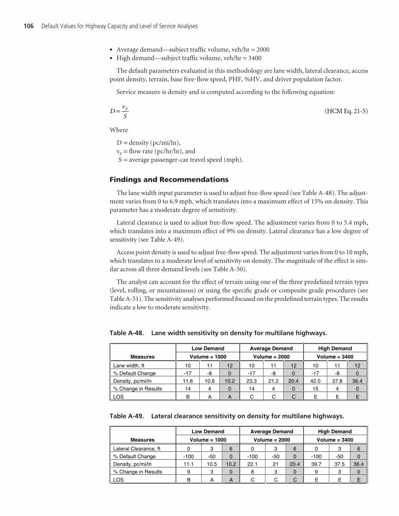
• Average demand—subject traffic volume, veh/hr = 2000• High demand—subject traffic volume, veh/hr = 3400
The default parameters evaluated in this methodology are lane width, lateral clearance, accesspoint density, terrain, base free-flow speed, PHF, %HV, and driver population factor.
Service measure is density and is computed according to the following equation:
Where
D = density (pc/mi/ln),vp = flow rate (pc/hr/ln), andS = average passenger-car travel speed (mph).
Findings and Recommendations
The lane width input parameter is used to adjust free-flow speed (see Table A-48). The adjust-ment varies from 0 to 6.9 mph, which translates into a maximum effect of 15% on density. Thisparameter has a moderate degree of sensitivity.
Lateral clearance is used to adjust free-flow speed. The adjustment varies from 0 to 5.4 mph,which translates into a maximum effect of 9% on density. Lateral clearance has a low degree ofsensitivity (see Table A-49).
Access point density is used to adjust free-flow speed. The adjustment varies from 0 to 10 mph,which translates to a moderate level of sensitivity on density. The magnitude of the effect is sim-ilar across all three demand levels (see Table A-50).
The analyst can account for the effect of terrain using one of the three predefined terrain types(level, rolling, or mountainous) or using the specific grade or composite grade procedures (seeTable A-51). The sensitivity analyses performed focused on the predefined terrain types. The resultsindicate a low to moderate sensitivity.
Dv
Sp= (HCM Eq. 21-5)
106 Default Values for Highway Capacity and Level of Service Analyses
Low Demand Average Demand High Demand
Measures Volume = 1000 Volume = 2000 Volume = 3400
Lane width, ft 10 11 12 10 11 12 10 11 12
% Default Change -17 -8 0 -17 -8 0 -17 -8 0
Density, pc/mi/ln 11.6 10.6 10.2 23.3 21.2 20.4 42.0 37.8 36.4
% Change in Results 14 4 0 14 4 0 15 4 0
LOS B A A C C C E E E
Table A-48. Lane width sensitivity on density for multilane highways.
Low Demand Average Demand High Demand
Measures Volume = 1000 Volume = 2000 Volume = 3400
Lateral Clearance, ft 0 3 6 0 3 6 0 3 6
% Default Change -100 -50 0 -100 -50 0 -100 -50 0
Density, pc/mi/ln 11.1 10.5 10.2 22.1 21 20.4 39.7 37.5 36.4
% Change in Results 9 3 0 8 3 0 9 3 0
LOS B A A C C C E E E
Table A-49. Lateral clearance sensitivity on density for multilane highways.
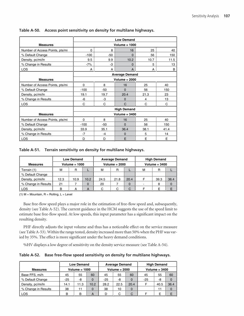
Sensitivity Analysis 107
Base free-flow speed plays a major role in the estimation of free-flow speed and, subsequently,density (see Table A-52). The current guidance in the HCM suggests the use of the speed limit toestimate base free-flow speed. At low speeds, this input parameter has a significant impact on theresulting density.
PHF directly adjusts the input volume and thus has a noticeable effect on the service measure(see Table A-53). Within the range tested, density increased more than 50% when the PHF was var-ied by 35%. The effect is more significant under the heavy demand conditions.
%HV displays a low degree of sensitivity on the density service measure (see Table A-54).
Low Demand
Measures Volume = 1000
Number of Access Points, pts/mi 0 8 16 25 40
% Default Change -100 -50 0 56 150
Density, pc/mi/ln 9.5 9.9 10.2 10.7 11.5
% Change in Results -7% -3 0 5 13
LOS A A A A B
Average Demand
Measures Volume = 2000
Number of Access Points, pts/mi 0 8 16 25 40
% Default Change -100 -50 0 56 150
Density, pc/mi/ln 19.1 19.7 20.4 21.3 23
% Change in Results -6 -3 0 4 13
LOS C C C C C
High Demand
Measures Volume = 3400
Number of Access Points, pts/mi 0 8 16 25 40
% Default Change -100 -50 0 56 150
Density, pc/mi/ln 33.9 35.1 36.4 38.1 41.4
% Change in Results -7 -4 0 5 14
LOS D D E E E
Table A-50. Access point sensitivity on density for multilane highways.
Low Demand Average Demand High Demand
Measures Volume = 1000 Volume = 2000 Volume = 3400
Terrain (1) M R L M R L M R L
% Default Change
Density, pc/mi/ln 12.3 10.9 10.2 24.5 21.8 20.4 F 39.3 36.4
% Change in Results 21 7 0 20 7 0 - 8 0
LOS B A A C C C F E E
(1) M = Mountain, R = Rolling, L = Level
Table A-51. Terrain sensitivity on density for multilane highways.
Low Demand Average Demand High Demand
Measures Volume = 1000 Volume = 2000 Volume = 3400
Base FFS, mi/h 45 55 60 45 55 60 45 55 60
% Default Change -25 -8 0 -25 -8 0 -25 -8 0
Density, pc/mi/ln 14.1 11.3 10.2 28.2 22.5 20.4 F 40.5 36.4
% Change in Results 38 11 0 38 10 0 11 0
LOS B B A D C C F E E
Table A-52. Base free-flow speed sensitivity on density for multilane highways.

Driver population factor is a flow rate adjustment factor. The sensitivity analyses show that den-sity is moderately sensitive to the variation of driver population (see Table A-55). Despite this find-ing, the current default values are adopted from research efforts in Florida. It may be appropriateto consider other local data sources.
Basic Freeway Segments
Part II of HCM 2000 lists default values for eight input parameters related to a basic freeway seg-ment. Of these eight input parameters, the length of analysis period does not enter into the method-ology and therefore was not included in the sensitivity analyses. Effects of the other seven inputparameters on the performance measure (density) were evaluated under low, average, and hightraffic congestion conditions. Each sensitivity analysis began with a base scenario. Values for theinput parameter were varied to record its effects. The input parameters are listed in Table A-56,followed by a summary of the base scenario.
Base Scenario
• PHF = 0.92• Percent of trucks and buses = 5%• Percent of recreational vehicles = 2%• Number of lanes in each direction = 3• Driver type = commuter• Terrain = level
108 Default Values for Highway Capacity and Level of Service Analyses
Low Demand Average Demand High Demand
Measures Volume = 1000 Volume = 2000 Volume = 3400
PHF 0.6 0.8 0.92 1 0.6 0.8 0.92 1 0.6 0.8 0.92 1
% Default Change -35 -13 0 9 -35 -13 0 9 -35 -13 0 9
Density, pc/mi/ln 15.7 11.8 10.2 9.4 32.1 23.5 20.4 18.8 F 43.5 36.4 32.9
% Change in Results 54 16 0 -8 57 15 0 -8 20 0 -10
LOS B B A A D C C C F E E D
Table A-53. PHF sensitivity on density for multilane highways.
Low Demand Average Demand High Demand
Measures Volume = 1000 Volume = 2000 Volume = 3400
%Heavy Vehicles 0 5 15 25 0 5 15 25 0 5 15 25
% Default Change -100 0 200 400 -100 0 200 400 -100 0 200 400
Density, pc/mi/ln 10 10.2 10.7 11.2 20 20.4 21.4 22.4 35.3 36.4 38.6 40.9
% Change in Results -2 0 5 10 -2 0 5 10 -3 0 6 12
LOS A A A B C C C C E E E E
Table A-54. %HV sensitivity on density for multilane highways.
Low Demand Average Demand High Demand
Measures Volume = 1000 Volume = 2000 Volume = 3400
Driver Population Factor 0.85 0.90 0.95 1.00 0.85 0.90 0.95 1.00 0.85 0.90 0.95 1.00
% Default Change -15 -10 -5 0 -15 -10 -5 0 -15 -10 -5 0
Density, pc/mi/ln 12 11.4 10.8 10.2 24.1 22.7 21.5 20.4 F 41.6 38.8 36.4
% Change in Results 18 12 6 0 18 11 5 0 14 7 0
LOS B B A A C C C C F F E E
Table A-55. Driver population sensitivity on density for multilane highways.
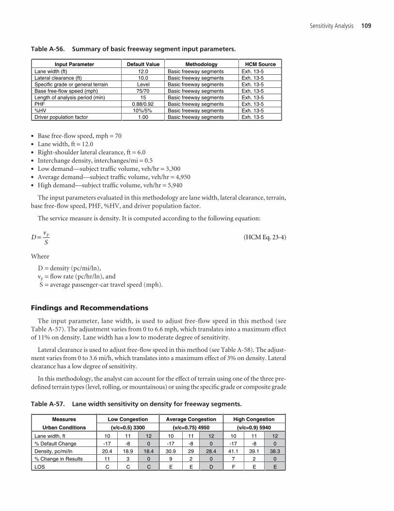
Sensitivity Analysis 109
• Base free-flow speed, mph = 70• Lane width, ft = 12.0• Right-shoulder lateral clearance, ft = 6.0• Interchange density, interchanges/mi = 0.5• Low demand—subject traffic volume, veh/hr = 3,300• Average demand—subject traffic volume, veh/hr = 4,950• High demand—subject traffic volume, veh/hr = 5,940
The input parameters evaluated in this methodology are lane width, lateral clearance, terrain,base free-flow speed, PHF, %HV, and driver population factor.
The service measure is density. It is computed according to the following equation:
Where
D = density (pc/mi/ln),vp = flow rate (pc/hr/ln), andS = average passenger-car travel speed (mph).
Findings and Recommendations
The input parameter, lane width, is used to adjust free-flow speed in this method (see Table A-57). The adjustment varies from 0 to 6.6 mph, which translates into a maximum effectof 11% on density. Lane width has a low to moderate degree of sensitivity.
Lateral clearance is used to adjust free-flow speed in this method (see Table A-58). The adjust-ment varies from 0 to 3.6 mi/h, which translates into a maximum effect of 3% on density. Lateralclearance has a low degree of sensitivity.
In this methodology, the analyst can account for the effect of terrain using one of the three pre-defined terrain types (level, rolling, or mountainous) or using the specific grade or composite grade
Dv
Sp= (HCM Eq. 23-4)
Measures Low Congestion Average Congestion High Congestion
Urban Conditions (v/c=0.5) 3300 (v/c=0.75) 4950 (v/c=0.9) 5940
Lane width, ft 10 11 12 10 11 12 10 11 12
% Default Change -17 -8 0 -17 -8 0 -17 -8 0
Density, pc/mi/ln 20.4 18.9 18.4 30.9 29 28.4 41.1 39.1 38.3
% Change in Results 11 3 0 9 2 0 7 2 0
LOS C C C E E D F E E
Table A-57. Lane width sensitivity on density for freeway segments.
Input Parameter Default Value Methodology HCM Source Lane width (ft) 12.0 Basic freeway segments Exh. 13-5 Lateral clearance (ft) 10.0 Basic freeway segments Exh. 13-5 Specific grade or general terrain Level Basic freeway segments Exh. 13-5 Base free-flow speed (mph) 75/70 Basic freeway segments Exh. 13-5 Length of analysis period (min) 15 Basic freeway segments Exh. 13-5 PHF 0.88/0.92 Basic freeway segments Exh. 13-5 %HV 10%/5% Basic freeway segments Exh. 13-5 Driver population factor 1.00 Basic freeway segments Exh. 13-5
Table A-56. Summary of basic freeway segment input parameters.

procedures (see Table A-59). The sensitivity analyses performed focused on the predefined terraintypes. The results indicate that the density has a significant degree of sensitivity to the terrain type.
According to the HCM, base free-flow speed plays a major role in the estimation of free-flowspeed and, subsequently, density. Despite this, the analyses indicate a low degree of sensitivity(see Table A-60).
PHF directly adjusts the input volume and thus has a noticeable effect on the service measure(see Table A-61). Within the range tested, density increased more than 50% when the PHF wasvaried by 35%. The effect is slightly more significant under the heavy congestion conditions.
%HV displays a low to moderate degree of sensitivity (see Table A-62).
Driver population factor is a flow rate adjustment factor (see Table A-63). The density is mod-erately sensitive to the variation of driver population factor under low traffic congestion condi-tions and highly sensitive under heavy traffic conditions.
Ramps and Ramp Junctions
There are two distinct methods in this chapter: one for the analysis of a merge influence areaand the other for the analysis of a diverge influence area. Part II of the HCM lists default valuesfor six input parameters related to ramp merge/diverge areas. Except for the acceleration anddeceleration lengths, the other four parameters are inputs to both methods. Although it is an input
110 Default Values for Highway Capacity and Level of Service Analyses
Low Congestion Average Congestion High Congestion
Measures (v/c=0.5) 3300 (v/c=0.75) 4950 (v/c=0.9) 5940
Lateral Clearance, ft 0 3 6 0 3 6 0 3 6
% Default Change -100 -50 0 -100 -50 0 -100 -50 0
Density, pc/mi/ln 19 18.7 18.4 29.2 28.8 28.4 39.3 38.8 38.3
% Change in Results 3 2 0 3 1 0 3 1 0
LOS C C C E E D E E E
Table A-58. Lateral clearance sensitivity on density for freeway segments.
Low Congestion Average Congestion High Congestion
Measure (v/c=0.5) 3300 (v/c=0.75) 4950 (v/c=0.9) 5940Terrain (1) M R L M R L M R L
% Default Change
Density, pc/mi/ln 22.0 19.5 18.4 38.3 31 28.4 >45 44.3 38.3
% Change in Results 20 6 0 35 9 0 - 16 0
LOS C C C F E D F E E
(1) M = Mountain, R= Rolling, L = Level
Table A-59. Terrain sensitivity on density at freeway segments.
Low Congestion Average Congestion High Congestion
Measures (v/c=0.5) 3300 (v/c=0.75) 4950 (v/c=0.9) 5940
Base FFS, mph 70 73 75 70 73 75 70 73 75
% Default Change 0 4 7 0 4 7 0 4 7
Density, pc/mi/ln 18.4 17.6 16.4 28.4 27.4 26.3 38.3 37.1 36.5
% Change in Results 0 -4 -11 0 -4 -7 0 -3 -5
LOS C C B D D D E E E
Table A-60. Base free-flow speed sensitivity on density at freeway segments.
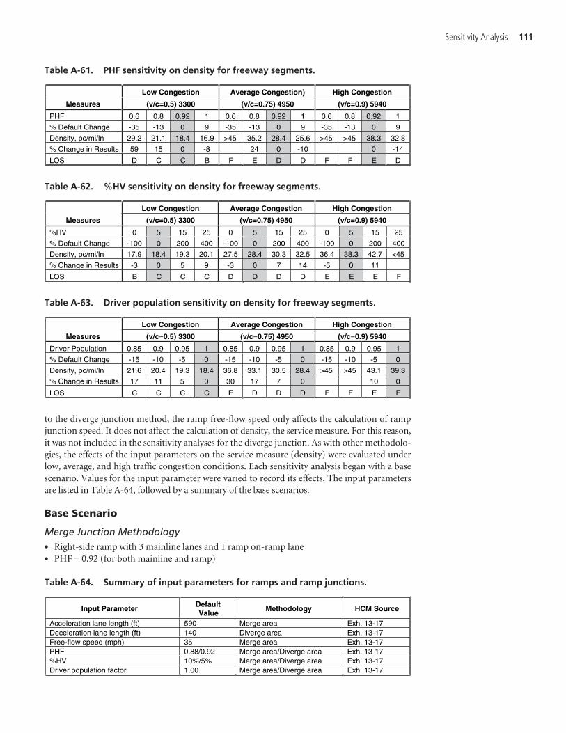
Sensitivity Analysis 111
to the diverge junction method, the ramp free-flow speed only affects the calculation of rampjunction speed. It does not affect the calculation of density, the service measure. For this reason,it was not included in the sensitivity analyses for the diverge junction. As with other methodolo-gies, the effects of the input parameters on the service measure (density) were evaluated underlow, average, and high traffic congestion conditions. Each sensitivity analysis began with a basescenario. Values for the input parameter were varied to record its effects. The input parametersare listed in Table A-64, followed by a summary of the base scenarios.
Base Scenario
Merge Junction Methodology• Right-side ramp with 3 mainline lanes and 1 ramp on-ramp lane• PHF = 0.92 (for both mainline and ramp)
Low Congestion Average Congestion) High Congestion
Measures (v/c=0.5) 3300 (v/c=0.75) 4950 (v/c=0.9) 5940
PHF 0.6 0.8 0.92 1 0.6 0.8 0.92 1 0.6 0.8 0.92 1
% Default Change -35 -13 0 9 -35 -13 0 9 -35 -13 0 9
Density, pc/mi/ln 29.2 21.1 18.4 16.9 >45 35.2 28.4 25.6 >45 >45 38.3 32.8
% Change in Results 59 15 0 -8 24 0 -10 0 -14
LOS D C C B F E D D F F E D
Low Congestion Average Congestion High Congestion
Measures (v/c=0.5) 3300 (v/c=0.75) 4950 (v/c=0.9) 5940
%HV 0 5 15 25 0 5 15 25 0 5 15 25
% Default Change -100 0 200 400 -100 0 200 400 -100 0 200 400
Density, pc/mi/ln 17.9 18.4 19.3 20.1 27.5 28.4 30.3 32.5 36.4 38.3 42.7 <45
% Change in Results -3 0 5 9 -3 0 7 14 -5 0 11
LOS B C C C D D D D E E E F
Table A-61. PHF sensitivity on density for freeway segments.
Table A-62. %HV sensitivity on density for freeway segments.
Low Congestion Average Congestion High Congestion
Measures (v/c=0.5) 3300 (v/c=0.75) 4950 (v/c=0.9) 5940
Driver Population 0.85 0.9 0.95 1 0.85 0.9 0.95 1 0.85 0.9 0.95 1
% Default Change -15 -10 -5 0 -15 -10 -5 0 -15 -10 -5 0
Density, pc/mi/ln 21.6 20.4 19.3 18.4 36.8 33.1 30.5 28.4 >45 >45 43.1 39.3
% Change in Results 17 11 5 0 30 17 7 0 10 0
LOS C C C C E D D D F F E E
Table A-63. Driver population sensitivity on density for freeway segments.
Input Parameter DefaultValue
Methodology HCM Source
Acceleration lane length (ft) 590 Merge area Exh. 13-17 Deceleration lane length (ft) 140 Diverge area Exh. 13-17 Free-flow speed (mph) 35 Merge area Exh. 13-17 PHF 0.88/0.92 Merge area/Diverge area Exh. 13-17 %HV 10%/5% Merge area/Diverge area Exh. 13-17 Driver population factor 1.00 Merge area/Diverge area Exh. 13-17
Table A-64. Summary of input parameters for ramps and ramp junctions.
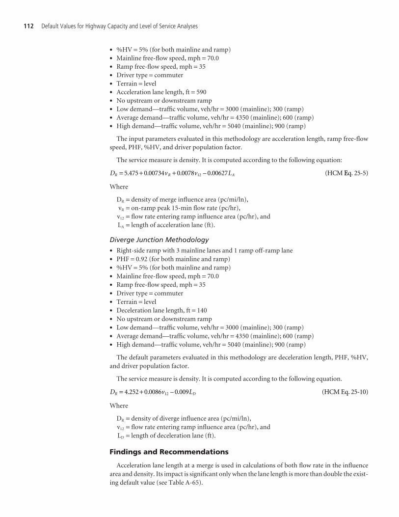
• %HV = 5% (for both mainline and ramp)• Mainline free-flow speed, mph = 70.0• Ramp free-flow speed, mph = 35• Driver type = commuter• Terrain = level• Acceleration lane length, ft = 590• No upstream or downstream ramp• Low demand—traffic volume, veh/hr = 3000 (mainline); 300 (ramp)• Average demand—traffic volume, veh/hr = 4350 (mainline); 600 (ramp)• High demand—traffic volume, veh/hr = 5040 (mainline); 900 (ramp)
The input parameters evaluated in this methodology are acceleration length, ramp free-flowspeed, PHF, %HV, and driver population factor.
The service measure is density. It is computed according to the following equation:
Where
DR = density of merge influence area (pc/mi/ln),vR = on-ramp peak 15-min flow rate (pc/hr),v12 = flow rate entering ramp influence area (pc/hr), andLA = length of acceleration lane (ft).
Diverge Junction Methodology
• Right-side ramp with 3 mainline lanes and 1 ramp off-ramp lane• PHF = 0.92 (for both mainline and ramp)• %HV = 5% (for both mainline and ramp)• Mainline free-flow speed, mph = 70.0• Ramp free-flow speed, mph = 35• Driver type = commuter• Terrain = level• Deceleration lane length, ft = 140• No upstream or downstream ramp• Low demand—traffic volume, veh/hr = 3000 (mainline); 300 (ramp)• Average demand—traffic volume, veh/hr = 4350 (mainline); 600 (ramp)• High demand—traffic volume, veh/hr = 5040 (mainline); 900 (ramp)
The default parameters evaluated in this methodology are deceleration length, PHF, %HV,and driver population factor.
The service measure is density. It is computed according to the following equation.
Where
DR = density of diverge influence area (pc/mi/ln),v12 = flow rate entering ramp influence area (pc/hr), andLD = length of deceleration lane (ft).
Findings and Recommendations
Acceleration lane length at a merge is used in calculations of both flow rate in the influencearea and density. Its impact is significant only when the lane length is more than double the exist-ing default value (see Table A-65).
D v LR D= +4 252 0 0086 0 00912. . – . (HCM Eq. 25-10)
D v v LR R A= + +5 475 0 00734 0 0078 0 0062712. . . – . (HCM EEq. 25-5)
112 Default Values for Highway Capacity and Level of Service Analyses
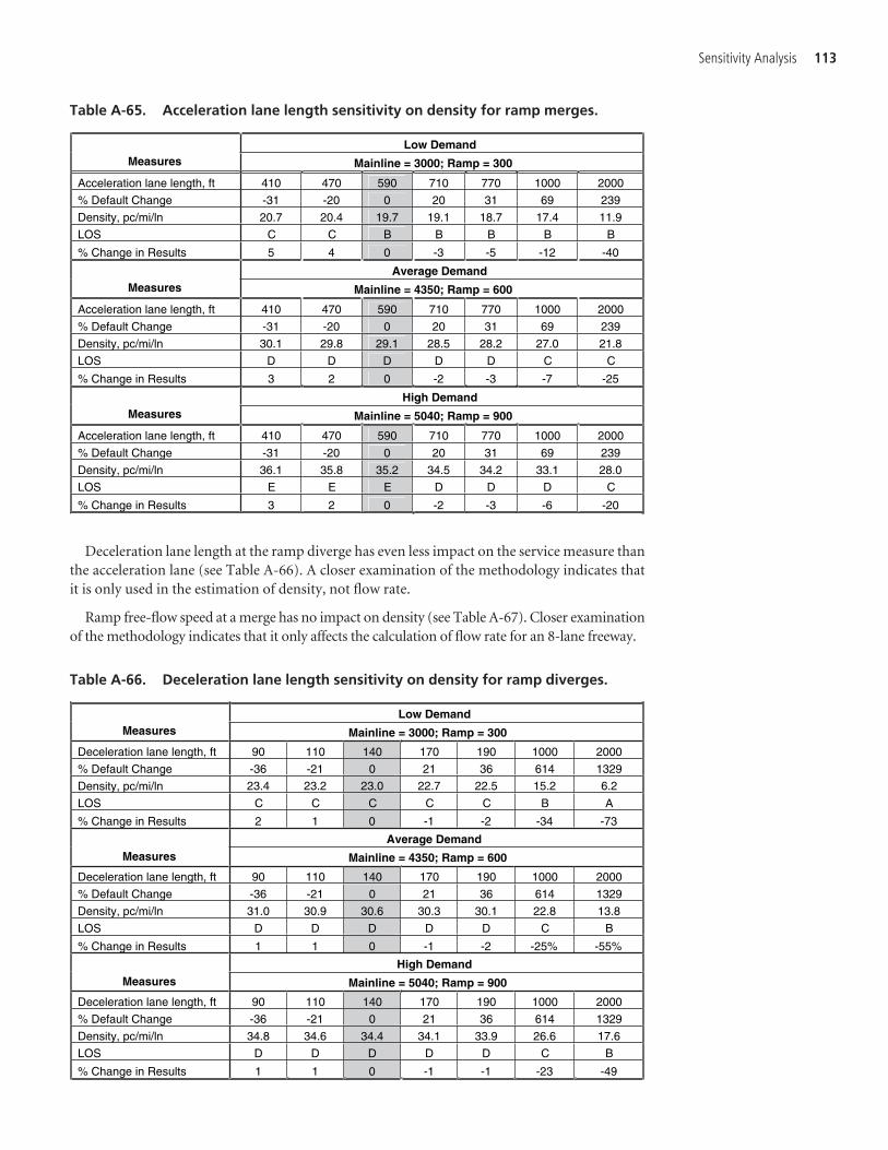
Sensitivity Analysis 113
Deceleration lane length at the ramp diverge has even less impact on the service measure thanthe acceleration lane (see Table A-66). A closer examination of the methodology indicates thatit is only used in the estimation of density, not flow rate.
Ramp free-flow speed at a merge has no impact on density (see Table A-67). Closer examinationof the methodology indicates that it only affects the calculation of flow rate for an 8-lane freeway.
Low Demand Measures Mainline = 3000; Ramp = 300
Acceleration lane length, ft 410 470 590 710 770 1000 2000
% Default Change -31 -20 0 20 31 69 239
Density, pc/mi/ln 20.7 20.4 19.7 19.1 18.7 17.4 11.9
LOS C C B B B B B
% Change in Results 5 4 0 -3 -5 -12 -40
Average Demand Measures Mainline = 4350; Ramp = 600
Acceleration lane length, ft 410 470 590 710 770 1000 2000
% Default Change -31 -20 0 20 31 69 239
Density, pc/mi/ln 30.1 29.8 29.1 28.5 28.2 27.0 21.8
LOS D D D D D C C
% Change in Results 3 2 0 -2 -3 -7 -25
High Demand Measures Mainline = 5040; Ramp = 900
Acceleration lane length, ft 410 470 590 710 770 1000 2000
% Default Change -31 -20 0 20 31 69 239
Density, pc/mi/ln 36.1 35.8 35.2 34.5 34.2 33.1 28.0
LOS E E E D D D C
% Change in Results 3 2 0 -2 -3 -6 -20
Table A-65. Acceleration lane length sensitivity on density for ramp merges.
Low Demand Measures Mainline = 3000; Ramp = 300
Deceleration lane length, ft 90 110 140 170 190 1000 2000
% Default Change -36 -21 0 21 36 614 1329
Density, pc/mi/ln 23.4 23.2 23.0 22.7 22.5 15.2 6.2
LOS C C C C C B A
% Change in Results 2 1 0 -1 -2 -34 -73
Average Demand Measures Mainline = 4350; Ramp = 600
Deceleration lane length, ft 90 110 140 170 190 1000 2000
% Default Change -36 -21 0 21 36 614 1329
Density, pc/mi/ln 31.0 30.9 30.6 30.3 30.1 22.8 13.8
LOS D D D D D C B
% Change in Results 1 1 0 -1 -2 -25% -55%
High Demand Measures Mainline = 5040; Ramp = 900
Deceleration lane length, ft 90 110 140 170 190 1000 2000
% Default Change -36 -21 0 21 36 614 1329
Density, pc/mi/ln 34.8 34.6 34.4 34.1 33.9 26.6 17.6
LOS D D D D D C B
% Change in Results 1 1 0 -1 -1 -23 -49
Table A-66. Deceleration lane length sensitivity on density for ramp diverges.

114 Default Values for Highway Capacity and Level of Service Analyses
Low Demand Measures Mainline = 3000; Ramp = 300
Ramp FFS, mi/h 20 30 35 40 50
% Default Change -43 -14 0 14 43
Density, pc/mi/ln 20 20 20 20 20
LOS B B B B B
% Change in Results 0 0 0 0 0
Average Demand Measures Mainline = 4350; Ramp = 600
Ramp FFS, mi/h 20 30 35 40 50
% Default Change -43 -14 0 14 43
Density, pc/mi/ln 29.1 29.1 29.1 29.1 29.1
LOS D D D D D
% Change in Results 0 0 0 0 0
High Demand Measures Mainline = 5040; Ramp = 900
Ramp FFS, mi/h 20 30 35 40 50
% Default Change -43 -14 0 14 43
Density, pc/mi/ln 35.2 35.2 35.2 35.2 35.2
LOS E E E E E
% Change in Results 0 0 0 0 0
Table A-67. Free-flow speed sensitivity on density for ramp merges.
Low Demand Average Demand High Demand
MergeMeasures
Mainline = 3000 Ramp = 300
Mainline = 4350 Ramp = 600
Mainline = 5040 Ramp = 900
Ramp PHF 0.6 0.8 0.92 1 0.6 0.8 0.92 1 0.6 0.8 0.92 1
% Default Change -35 -13 0 9 -35 -13 0 9 -35 -13 0 9
Density, pc/mi/ln 21.0 20.1 19.7 19.5 31.8 29.9 29.1 28.7 F 36.3 35.2 34.6
LOS C C B B D D D D F E E D
% Change in Results 7 2 0 -1 9 3 0 -1 3 0 -2
Low Demand Average Demand High Demand
Diverge
MeasuresMainline = 3000;
Ramp = 300Mainline = 4350
Ramp = 600Mainline = 5040
Ramp = 900
Ramp PHF 0.6 0.8 0.92 1 0.6 0.8 0.92 1 0.6 0.8 0.92 1
% Default Change -35 -13 0 9 -35 -13 0 9 -35 -13 0 9
Density, pc/mi/ln 23.3 23.1 23.0 22.9 31.3 30.8 30.6 30.5 35.5 34.7 34.4 34.2
LOS C C C C D D D D E D D D
% Change in Results 1 0 0 0 2 1 0 0 3 1 0 -1
Table A-68. PHF sensitivity on density for ramp merge and diverge.
Ramp PHF (merge and diverge methods) has less than 10% impact on the service measure(see Table A-68). This is because the flow rate (which is influenced by the PHF) is only one of the variables that influence the service measure (density). At all three demand levels evalu-ated, the impact was less significant for the diverge junction than for the merge junction.
In evaluating the effect of heavy vehicles, the %HV on the ramp was varied while the %HV onthe mainline remained the same. (The effect of heavy vehicles on the mainline was evaluated inBasic Freeway Segments subsection.) The analysis results indicate a low degree of sensitivity in boththe merge and the diverge methodologies (see Table A-69). This is because the flow rate (which isinfluenced by the %HV) is only one of the variables that influence the service measure (density).

Sensitivity Analysis 115
Driver population factor was assumed to be the same on the mainline and the ramp. There-fore, this input parameter was varied for both the mainline and the ramp at the same time. For exam-ple, a factor of 0.85 was applied to both the mainline and the ramp. The sensitivity results indicateda moderate degree of sensitivity (see Table A-70).
Conclusion
There are 63 input parameters in eight chapters of HCM 2000 for which default values are sug-gested. Seven of these input parameters are not used in the HCM methodologies. To determinewhere default values for these input parameters would be most significant, a sensitivity analysis wasconducted by applying a set of low, average, and high demands to each of these methodologies. Asa result of these, the default values were judged to have a low, moderate, or significant degree ofsensitivity in influencing the results. Table A-71 summarizes the sensitivity determined for each ofthese input parameters.
Low Demand Average Demand High Demand
MergeMeasures
Mainline = 3000Ramp= 300
Mainline = 4350 Ramp = 600
Mainline = 5040Ramp = 900
Ramp %HV 0 5 15 25 0 5 15 25 0 5 15 25
% Default Change -100 0 200 400 -100 0 200 400 -100 0 200 400
Density, pc/mi/ln 19.7 19.7 19.8 20.0 29.0 29.1 29.4 29.6 35.0 35.2 35.5 35.9
LOS B B B B D D D D D E E E
% Change in Results 0 0 1 2 0 0 1 2 -1 0 1 2
Low Demand Average Demand High Demand
Diverge
MeasuresMainline = 3000
Ramp = 300Mainline = 4350
Ramp = 600Mainline = 5040
Ramp = 900
Ramp %HV 0 5 15 25 0 5 15 25 0 5 15 25
% Default Change -100 0 200 400 -100 0 200 400 -100 0 200 400
Density, pc/mi/ln 23.0 23.0 23.0 23.0 30.6 30.6 30.6 30.6 34.3 34.4 34.5 34.5
LOS C C C C D D D D D D D D
% Change in Results 0 0 0 0 0 0 0 0 0 0 0 0
Low Demand Average Demand High Demand
MergeMeasures
Mainline = 3000 Ramp = 300
Mainline = 4350 Ramp = 600
Mainline = 5040 Ramp = 900
Driver Population Factor 0.85 0.9 0.95 1 0.85 0.9 0.95 1 0.85 0.9 0.95 1
% Default Change -15 -10 -5 0 -15 -10 -5 0 -15 -10 -5 0
Density, pc/mi/ln 22.9 21.7 20.7 19.7 34.0 32.2 30.6 29.1 F F 36.9 35.2
LOS C C C B D D D D F F E E
% Change in Results 16 10 5 0 17 11 5 0 5 0
Low Demand Average Demand High Demand
Diverge
MeasuresMainline = 3000
Ramp = 300Mainline = 4350
Ramp = 600Mainline = 5040
Ramp = 900
Driver Population Factor 0.85 0.9 0.95 1 0.85 0.9 0.95 1 0.85 0.9 0.95 1
% Default Change -15 -10 -5 0 -15 -10 -5 0 -15 -10 -5 0
Density, pc/mi/ln 26.0 24.9 23.9 23.0 34.3 33.0 31.7 30.6 38.4 36.9 35.6 34.4
LOS C C C C D D D D E E E D
% Change in Results 13 8 4 0 12 8 4 0 12 7 3 0
Table A-69. % HV sensitivity for density at ramps.
Table A-70. Driver population sensitivity on density for ramps.

Input Parameter Degree of Sensitivity General Traffic Characteristics
PHF Evaluated with individual chapters K Not evaluated D Not evaluated
Urban Streets Signal density (signals/mi) Significant Free-flow speed (mph) Low
Signalized Intersections
Exclusive turn lane required Used for geometric design, not for operational analysis
PHF Significant Length of analysis period (hr) Significant Arrival Type (AT) Significant
Adjusted Sat flow (veh/hr/ln) Significant when traffic demand approaches oversaturation
Base sat flow (pc/hr/ln) Significant when traffic demand approaches oversaturation
Lane widths (ft) Significant when traffic demand approaches oversaturation
%HV Significant Lane utilization (fLU) Significant Cycle length (sec) Moderate Lost time (sec/cycle) Moderate Parking maneuvers Moderate Unit extension time (sec) Low Actuated control adjustment factor (k) Low Upstream filtering adjustment factor (l) Low to moderate Grades Low to moderate Local bus frequency (buses stopping/hr) Low Pedestrians (peds/hr) Low
Pedestrians Effective sidewalk width (ft) Significant Street corner radius (ft) Significant Pedestrian walking speed (ft/s) Significant Pedestrian start-up time (s) Significant
Bicycles Paths PHF Significant Bicycle speed (mph) Significant Bicycle path width (ft) Not used in method
Multilane Highways Specific grade or general terrain Low to Moderate Base free flow speed (mph) Significant PHF Significant Lane width (ft) Moderate Access point density (points/mi) Moderate Driver population factor Moderate %HV Low Lateral clearance (ft) Low Length of analysis period (min) Not used in method
Two-Lane Highways
Length of passing lanes (mi) Low (% time spent-following) Moderate—Significant (travel speed)
Percent no-passing Low to moderate PHF Moderate
Lane width (ft) Low impact on speed; no impact on percent time-spent-following (PTSF)
Shoulder width (ft) Low impact on speed; no impact on PTSF
Access point density (points/mi) Low impact on speed; no impact on PTSF
Specific grade or general terrain Low %HV (trucks/buses) Low %HV (RVs) No impact Length of analysis period (min) Not used in method Directional split Not used in method
Table A-71. Summary of sensitivity of default parameters on service measures.
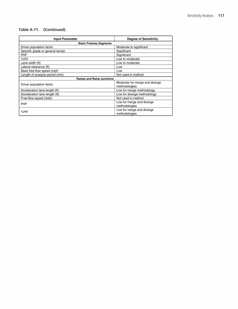
Sensitivity Analysis 117
Input Parameter Degree of Sensitivity Basic Freeway Segments
Driver population factor Moderate to significant Specific grade or general terrain Significant PHF Significant %HV Low to moderate Lane width (ft) Low to moderate Lateral clearance (ft) Low Base free-flow speed (mph Low Length of analysis period (min) Not used in method
Ramps and Ramp Junctions
Driver population factor Moderate for merge and diverge methodologies
Acceleration lane length (ft) Low for merge methodology Deceleration lane length (ft) Low for diverge methodology Free-flow speed (mph) Not used in method
PHFLow for merge and diverge methodologies
%HV Low for merge and diverge methodologies
Table A-71. (Continued).
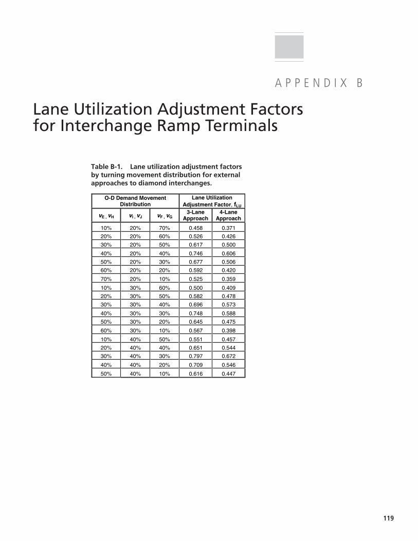
119
A P P E N D I X B
Lane Utilization Adjustment Factorsfor Interchange Ramp Terminals
O-D Demand Movement Distribution
Lane Utilization Adjustment Factor, fLU
vE , vH vI , vJ vF , vG3-Lane
Approach 4-Lane
Approach
10% 20% 70% 0.458 0.371
20% 20% 60% 0.526 0.426
30% 20% 50% 0.617 0.500
40% 20% 40% 0.746 0.606
50% 20% 30% 0.677 0.506
60% 20% 20% 0.592 0.420
70% 20% 10% 0.525 0.359
10% 30% 60% 0.500 0.409
20% 30% 50% 0.582 0.478
30% 30% 40% 0.696 0.573
40% 30% 30% 0.748 0.588
50% 30% 20% 0.645 0.475
60% 30% 10% 0.567 0.398
10% 40% 50% 0.551 0.457
20% 40% 40% 0.651 0.544
30% 40% 30% 0.797 0.672
40% 40% 20% 0.709 0.546
50% 40% 10% 0.616 0.447
Table B-1. Lane utilization adjustment factorsby turning movement distribution for externalapproaches to diamond interchanges.
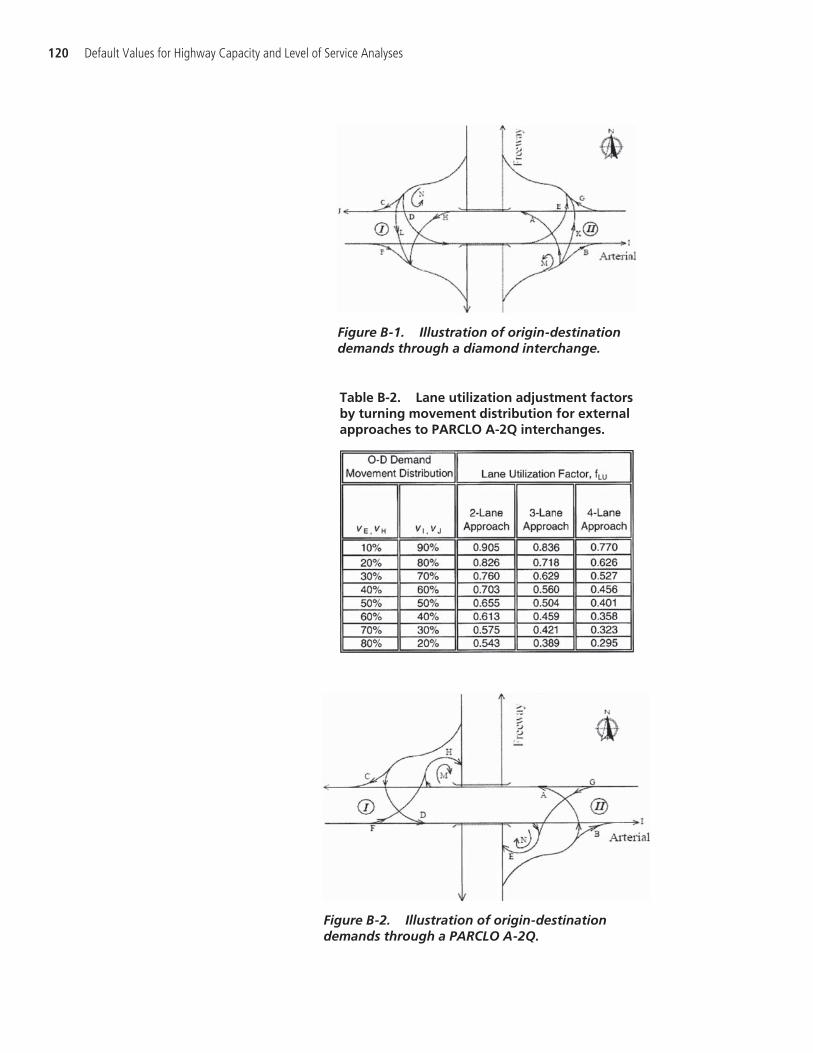
120 Default Values for Highway Capacity and Level of Service Analyses
Figure B-2. Illustration of origin-destinationdemands through a PARCLO A-2Q.
Table B-2. Lane utilization adjustment factorsby turning movement distribution for externalapproaches to PARCLO A-2Q interchanges.
Figure B-1. Illustration of origin-destinationdemands through a diamond interchange.
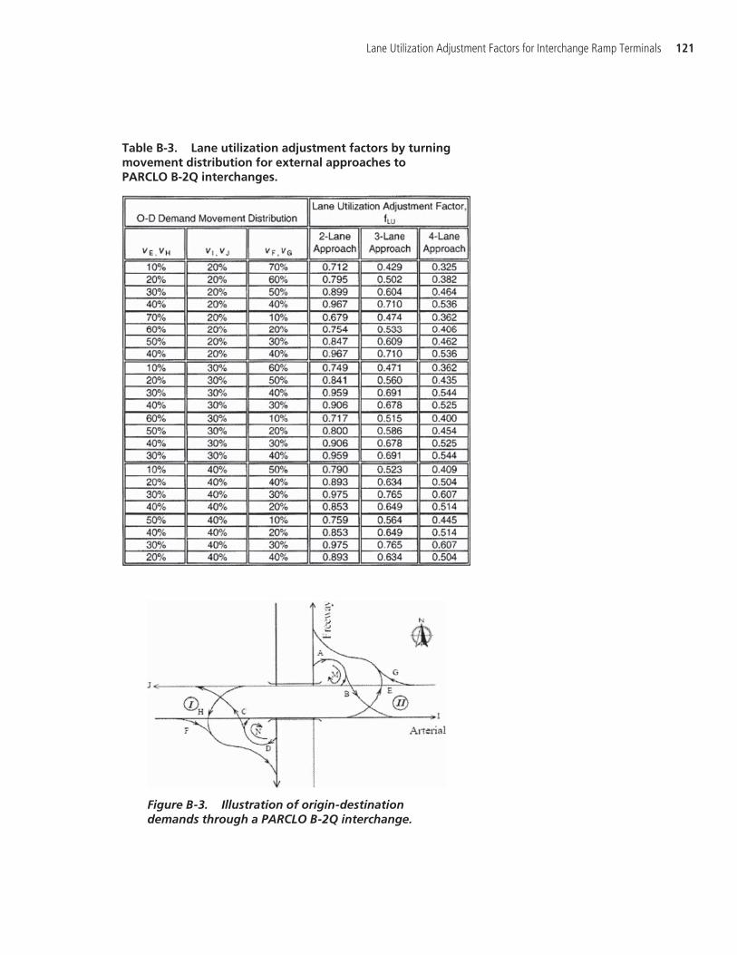
Lane Utilization Adjustment Factors for Interchange Ramp Terminals 121
Table B-3. Lane utilization adjustment factors by turningmovement distribution for external approaches to PARCLO B-2Q interchanges.
Figure B-3. Illustration of origin-destinationdemands through a PARCLO B-2Q interchange.
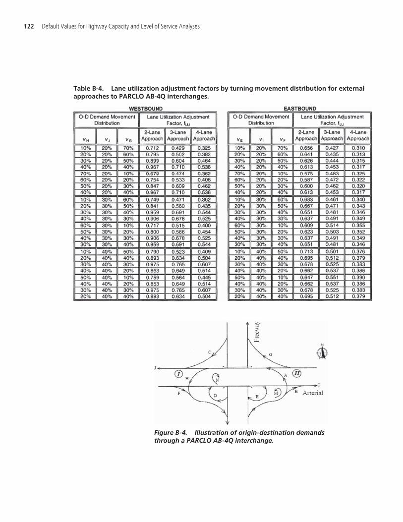
122 Default Values for Highway Capacity and Level of Service Analyses
Table B-4. Lane utilization adjustment factors by turning movement distribution for externalapproaches to PARCLO AB-4Q interchanges.
Figure B-4. Illustration of origin-destination demandsthrough a PARCLO AB-4Q interchange.
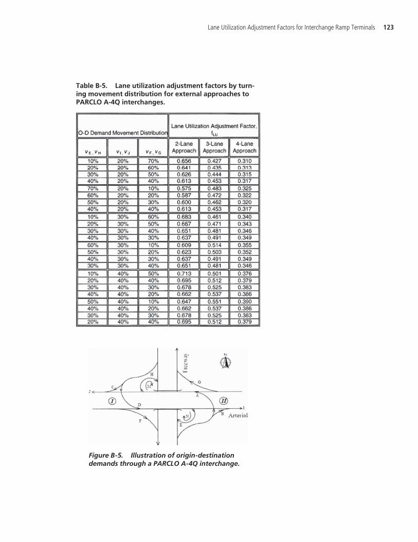
Lane Utilization Adjustment Factors for Interchange Ramp Terminals 123
Table B-5. Lane utilization adjustment factors by turn-ing movement distribution for external approaches toPARCLO A-4Q interchanges.
Figure B-5. Illustration of origin-destinationdemands through a PARCLO A-4Q interchange.

124 Default Values for Highway Capacity and Level of Service Analyses
Table B-6. Lane utilization adjustment factors by turning movement distribution for externalapproaches to PARCLO AB-2Q interchanges.
Figure B-6. Illustration of origin-destinationdemands through a PARCLO AB-2Q interchange.
Abbreviations and acronyms used without definitions in TRB publications:
AAAE American Association of Airport ExecutivesAASHO American Association of State Highway OfficialsAASHTO American Association of State Highway and Transportation OfficialsACI–NA Airports Council International–North AmericaACRP Airport Cooperative Research ProgramADA Americans with Disabilities ActAPTA American Public Transportation AssociationASCE American Society of Civil EngineersASME American Society of Mechanical EngineersASTM American Society for Testing and MaterialsATA Air Transport AssociationATA American Trucking AssociationsCTAA Community Transportation Association of AmericaCTBSSP Commercial Truck and Bus Safety Synthesis ProgramDHS Department of Homeland SecurityDOE Department of EnergyEPA Environmental Protection AgencyFAA Federal Aviation AdministrationFHWA Federal Highway AdministrationFMCSA Federal Motor Carrier Safety AdministrationFRA Federal Railroad AdministrationFTA Federal Transit AdministrationIEEE Institute of Electrical and Electronics EngineersISTEA Intermodal Surface Transportation Efficiency Act of 1991ITE Institute of Transportation EngineersNASA National Aeronautics and Space AdministrationNASAO National Association of State Aviation OfficialsNCFRP National Cooperative Freight Research ProgramNCHRP National Cooperative Highway Research ProgramNHTSA National Highway Traffic Safety AdministrationNTSB National Transportation Safety BoardSAE Society of Automotive EngineersSAFETEA-LU Safe, Accountable, Flexible, Efficient Transportation Equity Act: A Legacy for Users (2005)TCRP Transit Cooperative Research ProgramTEA-21 Transportation Equity Act for the 21st Century (1998)TRB Transportation Research BoardTSA Transportation Security AdministrationU.S.DOT United States Department of Transportation