NCAR/TN-289+IA Introduction to the CCM Modular Processor

NCAR/TN-289+IANCAR TECHNICAL NOTE

July 1987

Introduction to theCCM Modular Processor(Version PROC02)

MICHAEL A. DIAS

CLIMATE AND GLOBAL DYNAMICS DIVISION

NATIONAL CENTER FOR ATMOSPHERIC RESEARCHBOULDER. COLORADO

I

I - |

--I

I

CONTENTS

List of Figures . . . . . . . . . . . . . . . . . . . . . . . . . . . . vPreface . . . . . . . . . . . . . . . .. . . . . .... . . . . . . . vii

1.0 Introduction . . . . . . . . . . . . . . . . . . . . . . . . . . . .. 1

2.0 A Generic Processor Job Deck ..................... 32.1 Accessing the Generic Processor Job Deck ... . . . . . . . . . . . 32.2 Processor JCL . . . . . . . . . . . . . . . . . . . . . . . . . . 72.3 Processor Source Codes .................. . . .82.4 Input Control Parameters . . . . . . . . . . . . . . . 82.5 Jobstepping ........................ . 9

3.0 Use of Input Control Parameters . . . . . . . . . . . . . .. 103.1 Rules for Using Input Control Parameters ... . . . . . . . . . . . 103.2 Examples of Common Combinations of ICPs ... . . . . . . . . . . 123.3 A Brief List of Processor Options ... . . . . . . . . . . ..... 273.4 A List of Available Fields for Processing ... . . . . . . . . . . 423.5 User-defined Derived Fields . ................... 463.6 Accessing the Online Documentation ... . . . . . . . . . . . . . 48

4.0 Processor Output . . . . . . . . . . . . . . . . . . . . . . . . . . . 494.1 Graphical Output . . ... . . . . . . . . . . . . . . . 494.2 Printed Output . . . . . . . . . . . . . . . . . . . . . . . . .. 494.3 Save Tape Output ............ ........... 50

5.0 Summary . . . . . . . . . . . . . . . . . . . . 58

References . . . . . . . . . . . . . . . . . . . . . 59

iii111

I

List of Figures

Data Flow through the processor .................... 2

Printout from the generic job deck ................. . 51

Horizontal cross-section plot of temperature at 500 mb ........... 56

Latitudinal cross-section plot of the zonally averaged temperature field . . . . 57

V

Fig. 1.

Fig. 2a-e.

Fig. 3.

Fig. 4.

Preface

This technical note provides an introduction to the CCM Modular Processor, a post-

processing software package for the analysis of data on history tapes (mass storage volumes)

output by the NCAR Community Climate Model (CCM). This document is designed as

a tutorial to teach new users how to access the processor and complete simple tasks, and

as a quick reference guide for more experienced users. This introduction/tutorial is not a

comprehensive description of the modular processor.

ii

INTRODUTION TO THE CCM MODULAR PROCESSOR

1.0 Introduction

The CCM modular processor is a tool for the analysis of data on history tapes (massstorage files) output by the NCAR Community Climate Model (CCM). The data on thesefiles are input to the processor, manipulated, and output in various forms, according to aseries of user-specified requests. Requests are input by the user in card image form. Theprocessor is capable of perfoming the following functions:

1) Analysis of Individual Days (including time series)2) Time Averaging3) Ensemble Averaging4) Time Filtering5) Case Comparison6) Zonal Averaging7) Meridional Averaging8) Vertical Averaging9) Horizontal Area Averaging

10) Horizontal Plotting11) Meridional Cross-Section Ploting12) Latitudinal Cross-Section Ploting13) Time Series Plotting14) Color Plotting15) Computing New Fields16) Spectral Operations

a. Bandpass Filteringb. Horizontal Interpolationc. Spectral Graphics

Many types of data input into the processor are allowed. These include historytapes, either generated by the model or by another program, and certain types of savetapes generated by the processor. These include:

* history tapes,* time average save tapes,* time series save tapes,* time series plot save tapes.

The processor also outputs all of the above tape types. Additionally,the processor alsooutputs another type of save tape, one which contains only horizontal slices, and is referredto as a horizontal slice save tape. This type of tape has insufficient information to be ableto be input back into the processor, and is available for users who wish to do further post-processing of their own design. Figure 1 summarizes the data flow through the processor.

1

The processor is supported by the CCM Core Group, including updates to processor

capabilities, support for initial instruction in the use of the processor, and documentation

to assist users of all levels. This introductory document is not a comprehensive description

of the modular processor, but an introduction to assist users in the 'nuts and bolts' of ac-

cessing and using the processor. This will enable the new user to begin using the processor,

complete simple tasks, and introduce more detailed documentation about the Processor

(Wolski, 1987). That documentation should be referred to in order to understand and fully

utilize the processor.

Fig. 1. Data Flow through the Processor. Output from the CCM, in the form of history

tapes, is input to the processor. Depending on user requests, the output data may

take on any of the forms shown. History tapes, time average save tapes, time series

save tapes, and time series plot save tapes can be input back into the processor for

further processing. Horizontal slice save tapes are in a convenient form to input to

other user codes.

2

2.0 A Generic Processor Job Deck

This section introduces the processor by showing users how to acquire a copy of andrun a sample processor deck. This deck will familiarize users with the format of a processorrun deck. This deck can then be used as a template to build more complicated run decks.

2.1 Accessing the Generic Processor Job Deck

The modular processor is maintained as an executable image on the NCAR MassStore cartridge system. News about the modular processor (such as upgrades, knownbugs, new capabilites or a new version) and a sample job deck for running the processorare maintained on a virtual machine (account) on the NCAR IBM 4381 called CSMLIB.Assuming that you have a 4381 account, link to the CSMLIB virtual machine by invocationof the following command:

LINKTO CSMLIB <CR> (Note: <CR> denotes a carriage return)

and the system will respond with:

*** CSMLIB'S 191-DISK LINKED AS DASD nnn WITH FILEMODE m ***

where nnn is the device number assigned and m is the filemodeassociated with the CSMLIB files.

By typing

COPY CCMPROCA JOB m = = A <CR>

a copy of this file will be placed on your 191 (or A) disk.

Now enter:

REL m (DET <CR>

to release the CSMLIB disk.

The file you have just copied will look something like this:

3

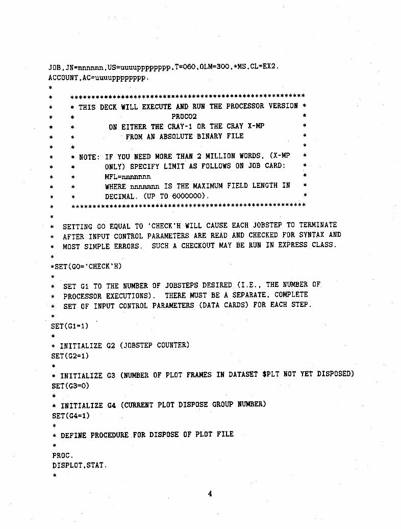
JOB,JN=nnnnn,US=uuuupppppppp,T=060,OLM=300,*MS,CL=EX2.

ACCOUNT,AC=uuuupppppppp.*

* ********************************************************

* * THIS DECK WILL EXECUTE AND RUN THE PROCESSOR VERSION *

* * PROC02 *

* * ON EITHER THE CRAY-1 OR THE CRAY X-MP *

* * FROM AN ABSOLUTE BINARY FILE *

* * *

* * NOTE: IF YOU NEED MORE THAN 2 MILLION WORDS, (X-MP *

* * ONLY) SPECIFY LIMIT AS FOLLOWS ON JOB CARD: *

* * MFL=nnnnnnn *

* * WHERE nnnnnnn IS THE MAXIMUM FIELD LENGTH IN *

* * DECIMAL. (UP TO 6000000). *

, ********************************************************

*

* SETTING GO EQUAL TO 'CHECK'H WILL CAUSE EACH JOBSTEP TO TERMINATE

* AFTER INPUT CONTROL PARAMETERS ARE READ AND CHECKED FOR SYNTAX AND

* MOST SIMPLE ERRORS. SUCH A CHECKOUT MAY BE RUN IN EXPRESS CLASS.

*

*SET(GO='CHECK'H)*

* SET Gi TO THE NUMBER OF JOBSTEPS DESIRED (I.E., THE NUMBER OF

* PROCESSOR EXECUTIONS). THERE MUST BE A SEPARATE, COMPLETE

* SET OF INPUT CONTROL PARAMETERS (DATA CARDS) FOR EACH STEP.

*

SET(Gl=I)*

* INITIALIZE G2 (JOBSTEP COUNTER)

SET(G2=1)*

* INITIALIZE G3 (NUMBER OF PLOT FRAMES IN DATASET $PLT NOT YET DISPOSED)

SET(G3=0)*

* INITIALIZE G4 (CURRENT PLOT DISPOSE GROUP NUMBER)

SET(G4=1)*

* DEFINE PROCEDURE FOR DISPOSE OF PLOT FILE

*

PROC.

DISPLOT,STAT.*

4

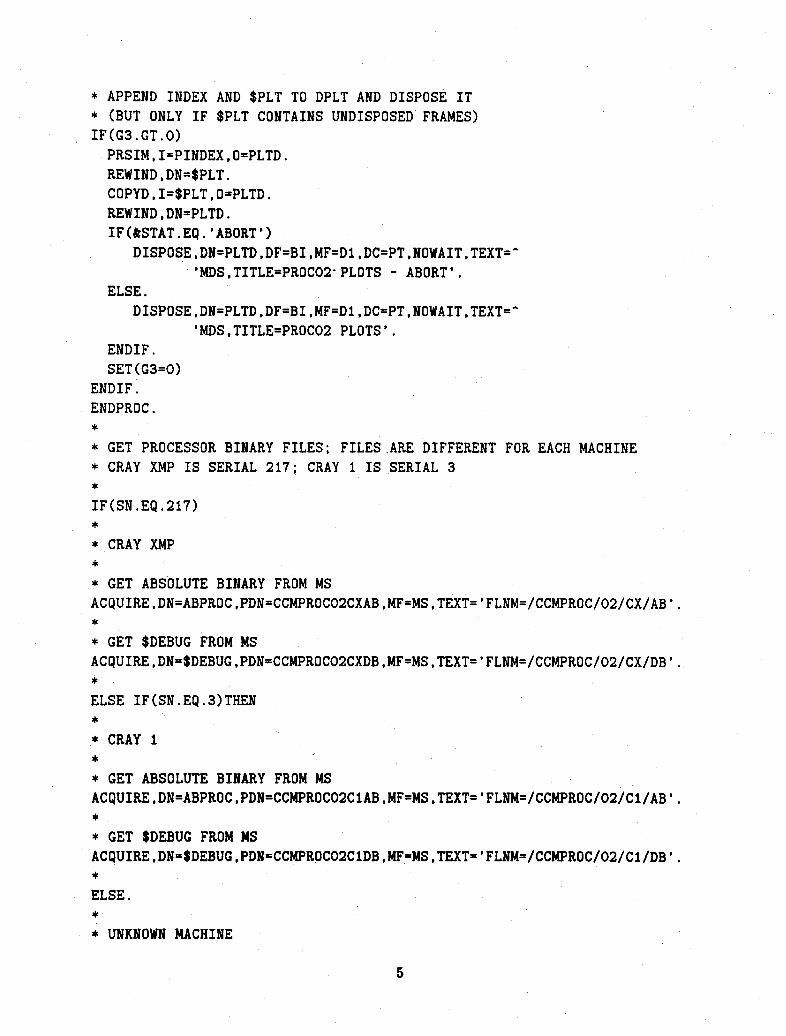
* APPEND INDEX AND $PLT TO DPLT AND DISPOSE IT* (BUT ONLY IF $PLT CONTAINS UNDISPOSED FRAMES)IF(G3.GT.O)

PRSIM,I=PINDEX,O=PLTD.

REWIND,DN=$PLT.

COPYD,I=$PLT,O=PLTD.

REWIND,DN=PLTD.

IF(&STAT.EQ.'ABORT')

DISPOSE,DN=PLTD,DF=BI,MF=D1,DC=PT,NOWAIT,TEXT= "

'MDS,TITLE=PROC02-PLOTS - ABORT'.

ELSE.

DISPOSE,DN=PLTD,DF=BI,MF=D1,DC=PT,NOWAIT,TEXT="

'MDS,TITLE=PROC02 PLOTS'.

ENDIF.SET(G3=0)

ENDIF.

ENDPROC.*

* GET PROCESSOR BINARY FILES; FILES.ARE DIFFERENT FOR EACH MACHINE* CRAY XMP IS SERIAL 217; CRAY I IS SERIAL 3*

IF(SN.EQ.217)

* CRAY XMP

*

* GET ABSOLUTE BINARY FROM MS

ACQUIRE,DN=ABPROC,PDN=CCMPROC02CXAB,MF=MS,TEXT='FLNM=/CCMPROC/02/CX/AB'.*

* GET $DEBUG FROM MS

ACQUIRE,DN=$DEBUG,PDN=CCMPROC02CXDB,MF=MS,TEXT='FLNM=/CCMPROC/02/CX/DB'.

ELSE IF(SN.EQ.3)THEN*

* CRAY 1

*

* GET ABSOLUTE BINARY FROM MS

ACQUIRE,DN=ABPROC,PDN=CCMPROC02C1AB.MF=MS.TEXT 'FLNM=/CCMPROC/02/C1/AB'.

* GET $DEBUG FROM MS

ACQUIRE,DN=$DEBUG,PDN=CCMPROC02C1DB,MF=MS,TEXT='FLNM=/CCMPROC/02/Cl/DB'.*

ELSE.

UNKNOWN ACHINE* UNKNOWN MACHINE

5

*

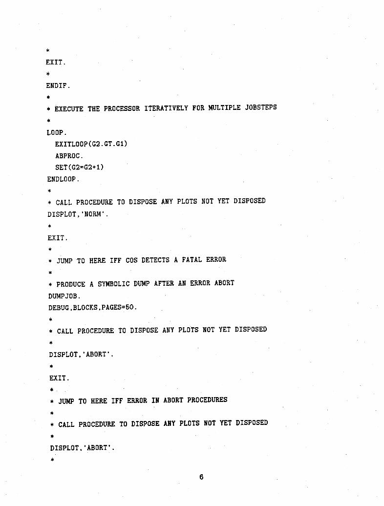
EXIT.

*

ENDIF.

*

* EXECUTE THE PROCESSOR ITERATIVELY FOR MULTIPLE JOBSTEPS

LOOP.

EXITLOOP(G2..GT.G1)

ABPROC.

SET(G2=G2+1)

ENDLOOP.

*

* CALL PROCEDURE TO DISPOSE ANY PLOTS NOT YET DISPOSED

DISPLOT,'NORM'.

*

EXIT.

*

* JUMP TO HERE IFF COS DETECTS A FATAL ERROR

*

* PRODUCE A SYMBOLIC DUMP AFTER AN ERROR ABORT

DUMPJOB.

DEBUG,BLOCKS,PAGES=50.

*


*

DISPLOT,'ABORT'.

*:

EXIT.

* .

* JUMP TO HERE IFF ERROR IN ABORT PROCEDURES

*


DISPLOT,'ABORT'.

*

6

\EOFC

C INPUT CONTROL PARAMETERS - JOB STEP 1C

C INPUT SPECIFICATIONSC

TITLEA='PROC02 TEST RUN'TAPESA='X22301'MSPFXI='/CSM/CCM1/223/'DAYSA=5.FIELDA1='T'

CC DATA MANIPULATION SPECIFICATIONSCPRESSLEV=900.,800.,700.,600.,500.,400.,300.,200.,100.

CC PLOT SPECIFICATIONSC

HPROJ='RECT'ZONAVG='YES'

CC PLOT OUTPUT SPECIFICATIONSC

DPLTMF='IO'DPLTFN='SAMPLE'DPLTFT='PLOTS'

CENDOFDATA

\EOF

Replacing uuuupppppppp by your own user ID and project number, and nnnnnn by yourown job or user name will provide you with a running JCL code for the processor. Thisdeck will process a small sample of a model history tape. After reading more of thistutorial, you can change other cards in this run deck, using this deck as a model to buildon.

2.2 Processor JCL

The CRAY JCL (job control language) deck is used to ACQUIRE and run the proces-sor code. The cards from SET(GO='CHECK'H) to SET(G4=1) set five Cray global pseudoregisters. These registers are a means by which the processor and the Cray Operating

7

System (COS) communicate information. G2, G3, and G4 should not be changed by the

user. The value of G1 determines how many times the processor is run, and should be ad-

justed by the user (instructions for determining this value will follow in section 2.5). The

SET((GO='CHECK'H) card can be uncommented (by deleting the '*' in column 1) if the user

wishes only to check the Input Control Parameters (see following section) for accuracy,

without processing the data.

Separate executable images of the code are maintained for the Cray-1 and the X-MP.

Depending upon the machine this is run on, the appropriate ACQUIRE statement in the JCL

gets the executable image for the processor code. The loop around the ABPROC statement

executes the processor repeatedly, according to the value of G1. Finally, there is a check

to DISPOSE any plots not yet disposed, according to the procedure defined earlier in the

JCL.

This procedure allows for control of the disposition of the graphical output, in this

case to the DICOMED microfiche film unit (MF=D1), if any plots were created. Since there

is a FORTRAN callable DISPOSE within the processor code, which defaults to a dispose to the

dicomed, these statements are not normally executed (disposition of output is discussed

in section 4). If this procedure is called with the ABORT condition set, the first DISPOSE is

executed, otherwise the second is executed.

2.3 Processor Source Code

The processor code can be modifed by the user, and a microfiche copy of the code

can be obtained from the Core Group. Those interested in modifying the processor should

consult the CCM Core Group.

2.4 Input Control Parameters

The Input Control Parameters (hereafter referred to as ICPs) are all the cards fol-

lowing the Cray JCL and preceding the last \EOF in the run deck. ICPs are the means by

which you specify what you want the processor to do. The sample ICP deck shown will

do the following:* read the T field from history tape /CSM/CCM1/223/X22301, (the Mass Store path-

name),* process day 0.0 from this tape,· interpolate input data to specified pressure levels,· compute and plot zonal averages of these fields,

· plot horizontal plots on all interpolated pressure levels for the above fields,

· dispose the plot file to the IBM 4381 as file SAMPLE PLOTS.

This is one of the simplest examples of an ICP deck. Rules for using ICPs and a

detailed discussion of this and other examples will be deferred to section 3.

8

2.5 Jobstepping

In cases where the processor cannot perform the task you wish to complete in onerun, capabilites exist for running multiple processor runs (or steps) within a single jobsubmission. Again, the statement SET(G1=1) sets the number of job steps (i.e. the numberof times the processor code is loaded and run). The binary image for the processor isexecuted repeatedly, according to the value of G1 (in this case, 1). This capability, calledjobstepping, often saves time submitting jobs which must be processed consecutively. Forexample, suppose the job to be performed is a composite of January averages. Withoutjobstepping, the composite averaging job would have to be submitted after all the singlejobs were completed. But, by jobstepping, each step could compute one January average,while the last step could compute the composite average. This technique can also be usedto avert unnecessary interaction with the Mass Store (by saving the results from one runon the CRAY disk and immediately re-accessing them, rather than disposing to the MassStore). Note the provision in the ICP jobstream for jobstepping, by separating two groupsof ICPs by an ENDOFDATA card (coincident with the value of Gl). This separates these twogroups of control parameters into two separate processor 'jobs' within the same job deck(each execution of the processor then uses the next deck of ICPs).

Summarizing, the basic structure of the submission deck for the modular processoris:

JOB CARD

CRAY JCL

\EOF

INPUT CONTROL PARAMETERS

ENDOFDATA

SECOND DECK OF INPUT CONTROL PARAMETERS

ENDOFDATA

\EOF

9

3.0 Use of Input Control Parameters

The best way to become familiar with the basic functions of the processor is to runa few simple jobs. This section will explain the rules for using ICPs (3.1), and some

common examples of ICP decks which perform specific functions (3.2). Following that is

a brief glossary of available keywords (3.3), a list of all fields available for processing (3.4),an introduction into the use of user-defined derived fields (3.5), and an introduction tofurther documentation available online(3.6).

3.1 Rules for Using Input Control Parameters

This section is intended to provide the user with some basic rules for using ICPs. Itis reccomended that the user read this section, then study the examples in section 3.2, and

then reread this section. The rules for using ICPs will make more sense to the user if this

sequence is followed.

The following job deck provides examples of how ICPs are used together to perform

a given processing task.

CC DEFINE PROCESSING FOR CASE A

CTITLEA='TEST RUN - CASE A'

MSPFXIA='M/SM/CCM1/223/TAPESA='X22301'

DAYSA=21.0,25.5,0.5FIELDA1='T','U', 'V', HT1,'Q'

TIMAVGA='YES'

CC COMPUTE, PLOT, AND PRINT ZONAL AVERAGES

C (USE SCALE FACTOR FOR MIXING RATIO PLOTS)

CZONAVG='YES'

ZAVGPRN='YES'

MXSCAL='Q',1.E8CC RECTANGULAR, HORIZONTAL PROJECTION PLOTS

CHPROJ='RECT'

CC DATA CARD TERMINATOR FOR THIS JOB STEP

CENDOFDATA

C---------------------------------------

C

10

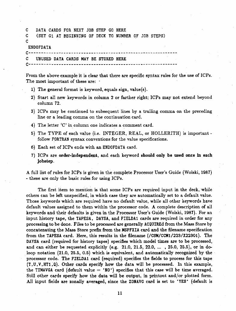
C DATA CARDS FOR NEXT JOB STEP GO HEREC (SET Gi AT BEGINNING OF DECK TO NUMBER OF JOB STEPS)C

ENDOFDATAC-----------______------------------C UNUSED DATA CARDS MAY BE STORED HEREC-- ---------------____--------_---__ --_--

From the above example it is clear that there are specific syntax rules for the use of ICPs.The most important of these are:

1) The general format is keyword, equals sign, value(s).

2) Start all new keywords in column 2 or farther right; ICPs may not extend beyondcolumn 72.

3) ICPs may be continued to subsequent lines by a trailing comma on the precedingline or a leading comma on the continuation card.

4) The letter 'C' in column one indicates a comment card.

5) The TYPE of each value (i.e. INTEGER, REAL, or HOLLERITH) is important -follow FORTRAN syntax conventions for the value specifications.

6) Each set of ICPs ends with an ENDOFDATA card.

7) ICPs are order-independent, and each keyword should only be used once in eachjobstep.

A full list of rules for ICPs is given in the complete Processor User's Guide (Wolski, 1987)- these are only the basic rules for using ICPs.

The first item to mention is that some ICPs are required input in the deck, whileothers can be left unspecified, in which case they are automatically set to a default value.Those keywords which are required have no default value, while all other keywords havedefault values assigned to them within the processor code. A complete description of allkeywords and their defaults is given in the Processor User's Guide (Wolski, 1987). For aninput history tape, the TAPESA, DAYSA, and FIELDA1 cards are required in order for anyprocessing to be done. Files to be processed are generally ACQUIREd from the Mass Store byconcatenating the Mass Store prefix from the MSPFXIA card and the filename specificationfrom the TAPESA card. Here, this results in the filename (/CSM/CCM1/223/X22301). TheDAYSA card (required for history tapes) specifies which model times are to be processed,and can either be requested explicitly (e.g. 21.0, 21.5, 22.0, ... , 25.0, 25.5), or in do-loop notation (21.0, 25.5, 0.5) which is equivalent, and automatically recognized by theprocessor code. The FIELDA1 card (required) specifies the fields to process for this tape(T,U,V,HT1 Q). Other cards specify how the data will be processed. In this example,the TIMAVGA card (default value = 'NO') specifies that this case will be time averaged.Still other cards specify how the data will be output, in printout and/or plotted form.All input fields are zonally averaged, since the ZONAVG card is set to 'YES' (default is

11

'NO'), and the results are printed in the output file, since ZAVGPRN='YES' (default is

'NO'). Further, the meridional cross-section plots are automatically produced for all fieldsif zonal averaging is done. MXSCAL defines the scaling of the contour labels for the fields

specified for the meridional cross-section plots (here,the labels for Q are scaled by a factor

of 1.E8). HPROJ='YES' (default is 'NO') specifies that horizontal projection plots for all

sigma levels are plotted on a cylindrical equidistant projection (rectangular). The TITLEA

card contains the user defined title for plots and printout of case A processing. The defaultis to produce no title.

Some ICPs end in an A, B, or C. Any ICP with such an ending is a case dependentICP. For comparison of two cases (or tapes), case A and B suffixes are used for data cardspertaining to these two tapes, and the case C suffix applies to the keywords pertainingeither to the comparison of cases A and B or to the merging of cases A and B. In the

no comparison case, case A is used for all case-dependent keywords. The TIMAVGA card

indicates that case A should be time averaged. Other cards, such as the FIELDA1 card,also have a numeric suffix. The numeric ending indicates a field pass dependent ICP. Field

passes allow the user to process input data over several field 'passes' of the input data, so

that enough memory is available for each pass of the data. The FIELDA1 card is also an

example of a field and case dependent ICP. Memory restrictions limit the number of fields

which can be processed in a single pass. Cards with no such suffix control processing for

all field passes and cases.

The comment cards following the ENDOFDATA mark the location of optional decks of

ICPs for jobstepping, with each deck being terminated by an ENDOFDATA card.

3.2 Examples of Common Combinations of ICPs

Many common processing jobs result from similar combinations of ICPs. These

common tasks can be copied, modified if necessary, and used for your own processingtasks (however, it is advised that you read the full description of each keyword in the

User's Guide before using it). Examples of common processing tasks are:

1) process one day for one case,2) produce a five-day time average,3) produce two ten-day time averages and compare them,4) recompute differences and plots from two save tapes,5) replot only differences from a save tape, respecifying contour intervals,6) compute standard deviations from 4 processor save tapes,7) produce two 5-day time averages and average the results (3 jobsteps).

The card decks for the examples listed above follow. Preceding each is a brief de-

scription of what each deck would produce. Following each is a description of the pertinent

new options introduced in the example. If these examples are run in sequence, they pro-vide examples which can be run as shown. All of the examples are contained in file

CCMPROC EXAMPLES on the CSMLIB machine (see section 2.1 for instructions on linking to

the CSMLIB disk).

12

Example 1 - Process one day.

This deck processes one model day for case A, interpolates to pressure surfaces,produces horizontal plots for each pressure level of each field, zonally averages the dataand prints out of the zonal averages (a total of 24 plots).

C EXAMPLE NO 1.C PROCESS 1 DAY (10.) FOR CASE AC

C SPECIFICATION CASE AC TITLE WILL APPEAR ON PRINTOUT RESULTS AND ON PLOTSC

TITLEA='CASE A DAY 10MSPFXIA='/CSM/CCM1/223/'TAPESA='X22301'DAYSA=10.0FIELDA1='T','Q','HT1'

CC INVOKE VERTICAL INTERPOLATION BY USE OF THE PRESSLE CARDC NOTE: DEFAULT IS SIGMA COORDINATESCPRESSLE=1000.,850.,700.,500.,300.,200.,100.

CC PRODUCE PLOTS BY USING THE HORIZONTAL PROJECTION OPTION HPROJCHPROJ='RECT'

CC SCALE FACTOR FOR MERIDIONAL CROSS-SECTION PLOT OF QCMXSCAL='Q',1.E8

CC COMPUTE AND PRINT THE ZONAL AVERAGESCZONAVG='YES'ZAVGPRN='YES'

CENDOFDATA

C--------- ---- ------------- ----- _----

Example 1 is the format to use for processing single days. The only difference betweenprocessing of single days or a time average is the value of TIMAVGA. TIMAVGA='NO', bydefault, and must be specified as 'YES' in order to produce a time average. The PRESSLEcard tells the processor to interpolate the input model sigma levels to the specified pressure

13

levels (in mb). There will be one zonal average plot produced for each field, and sevenhorizontal plots each for T, HT1, and Q. These plots are produced on microfiche on theDicomed plotting device by default.

In most cases, you will need to specify the Mass Store Path Name (MSPN) of the file

you wish to ACQUIRE. This is accomplished by the case-specific keyword MSPFXIA. Here, theMSPN is the concatenation of the prefix and the pathname, or /CSM/CCM1/223/X22301.Were there multiple tapes specified for Case A, the same prefix would have been appendedto each tape before acquiring it from the Mass Store. Refer to the Processor User's Guide

(Wolski, 1987) for a more complete description of Mass Store keywords (see topic *MSIN).

14

Example 2 - Produce a five-day time average.

The next deck produces a five day time average for case A, using do-loop notationto specify the days list. All other processing parallels that of example 1.

Note, for both examples, that if only one case is processed, case A is used for casedependent keywords. The HPROJ ICP controls all horizontal projection plotting, and whenZONAVG is set equal to 'YES', meridional cross-section plots are automatically created.For this example, 35 horizontal projection plots (5 X 7 pressure levels) and 5 meridionalcross-section plots are created.

C- ---------------------------------------------------C EXAMPLE NO 2.CC TIME AVERAGE OF 5 MODEL DAYS FOR CASE ACC SPECIFICATION OF CASE ACC TITLE WILL APPEAR ON PRINTOUT RESULTS AND ON PLOTSCTITLEA='CASE A 5 DAY AVG (21-25) '

MSPFXIA='/CSM/CCM1/223/'TAPESA='X22302'

CC DAYS LIST IS IN DO LOOP NOTATION AND IS EQUIVALENTC TO 21.0,21.5,22.0,22.5,23.0,23.5,24.0,24.5,25.0,25.5CDAYSA=21.0,25.5,0.5

CFIELDA1='T','U','V','Q','HT1'TIMAVGA='YES'

CC INVOKE VERTICAL INTERPOLATION BY USE OF THE PRESSLE CARD

C NOTE: DEFAULT IS SIGMA COORDINATESCPRESSLE=1000.,850.,700.,500.,300.,200.,100.

CC PRODUCE PLOTS BY USING THE HORIZONTAL PROJECTION OPTION HPROJC

HPROJ='RECT'CC SCALE FACTOR FOR MERIDIONAL CROSS- SECTION PLOT OF QC (SEE PAGE A-12 OF USERS' GUIDE)C

15

MXSCAL='Q',1.E8CC COMPUTE AND PRINT THE ZONAL AVERAGES

CZONAVG='YES'ZAVGPRN='YES'

CC SAVE THE RESULTS OF CASE A TO FILEA WITH WRITE PASSWORD WRPASS

C

SAVTAVA='FILEA','WRPASS'CENDOFDATA

Example 2 above is the format for time averaging a series of days. Do-loop notation is

used for the DAYSA specification. The time average can be saved on a Mass Store pathname

using the SAVTAVA keyword. The first parameter ('FILEA') is the filename, and the second

('WRPASS') is a write password assigned to the file. The file will be saved on the Mass

Store under the full file pathname /user/FILEA, where user is your username.

16

Example 3 - Produce two ten-day averages and compare them.

Example 3 uses the three case capability to process the difference between two 10-day averages. Each 10-day average is processed in the same manner as example 2, and thedifferences are requested for the field pass 1 fields by invoking the DIFFLD1 card. Thesefield lists are in the form case A field, case B field, user-specified difference field. Thedifferences are saved (SAVTAPC) to FILEC.

C- -- _____

C EXAMPLE NO 3.C

C AVERAGE AND DIFFERENCE OF 2 CASES (A AND B) FOR 10 MODEL DAYS

C

C SPECIFICATION OF CASE AC

C TITLE WILL APPEAR ON PRINTOUT RESULTS AND ON PLOTS

C

TITLEA='CASE A - 10 DAY AVG(MODEL DAYS 31-40)'

MSPFXIA='/CSM/CCM1/223/'TAPESA='X22303'

CC DAYS LIST IS IN DO LOOP NOTATION

C (PROCESSOR DAYS(MODEL TIMES) 31.0-40.5 INCLUSIVE)

CDAYSA=31.0,40.5,0.5

CFIELDA1='T','U','V'TIMAVGA='YES'

CC SAVE THE TIME AVERAGE OF CASE A TO FILEA WITH WRITE PASSWORD WRPASS

CSAVTAVA='FILEA','WRPASS'

C--------------------- -- ----------

CC SPECIFICATION OF CASE B

CTITLEB='CASE B 10 DAY AVG ( MODEL DAYS 61-70)'

MSPFXIB='/CSM/CCM1/223/'TAPESB='X22305'DAYSB=61.0,70.5,0.5FIELDBI='T','U','V'TIMAVGB='YES'

CC SAVE THE TIME AVERAGE OF CASE B TO FILEB WITH WRITE PASSWORD WRPASS

17

CSAVTAVB='FILEB','WRPASS'

C----.. _ _.. __ __ __-------------------.

CC COMPUTE THE DIFFERENCES FOR CASE A - CASE B FOR T AND

C HT1 ONLY

CDIFFLD1='T','T', 'TDIFF' ,U' 'U' 'UDIFF'

CC SAVE THE DIFFERENCE OF THE TIME AVERAGES TO FILEC

C WITH WRITE PASSWORD WRPASS

C

SAVTAVC='FILEC','WRPASS'C _-------------------------------------

CC PROCESSING OPTIONS FOR BOTH CASE A AND B

CC COMPUTE AND PRINT THE ZONAL AVERAGES

C

ZONAVG='YES'ZAVGPRN='YES'

CENDOFDATA

C----------- -- ------ -- -----------------

In example 3, all averages are computed on model sigma levels, since the PRESSLE keyword

is absent. The keywords ending in 'B' are case B keywords. These case-specific keywords

only apply to that case. The keywords ending in 'C' are the difference keywords (ratios

can also be computed in case C, using the RATFLDn keyword). The differences of the time

averaged case A temperature field minus the time averaged case B temperature field are

being computed and put in a field called 'TDIFF'. A similar computation is being done

for the u-wind field. The differences are then saved on a save tape.

One important point to note about the DIFFLDn keyword is that it is a field pass

specific keyword. This means that the differences computed are for the specific field pass

referred to in the keyword. For example, if FIELDA1 = 'T' and FIELDB1 = 'U', then the

card DIFFLD1='T'. 'T', 'TDIFF' is invalid, because the 'T' field for case B does not exist

on the FIELDB1 card.

18

Example 4 - Recompute differences and plots from two save tapes.

If the save tapes from the two cases already exist, you could use example 4 to computethe difference. FILEA and FILEB are two time-averaged save tapes, and if they were theones produced in example 3, this deck would produce the exactly the same results asexample 3, except that contour intervals for some fields and levels are specified explicitly,rather than selected automatically.

C ------ --- ---------------

C EXAMPLE NO 4.C

RECOMPUTE DIFFERENCES AND PLOTS OF 2 CASES (A AND B)

FOR 10 MODEL DAY AVERAGE FROM SAVES OF CASE A AND CASE B

C SPECIFICATION OF CASE A BY A SAVE TAPE

C

TITLEA='CASE A

C

C

C

C

10 DAY AVG(31-40)'

THE 10 MODEL DAY AVERAGE WAS SAVED IN PREVIOUS PROCESSOR

RUN (SEE EXAMPLE NO 3.) DAYSA AND TIMAVGA CONTROL PARAMETERS NOT

REQUIREDC

TYPEA='SAVTAV'C

TAPESA='FILEA'C

FIELDA1='T','U','V'C--------------------------

CC SPECIFICATION OF CASE B BY A SAVE TAPE

C

TITLEB='CASE B

TYPEB='SAVTAV'TAPESB='FILEB'FIELDB1='T','U','V

10 DAY AVG(61-70)'

C

CC

C COMPUTE DIFFERENCES OF T,HT1 AND U FROM CASES A - B

CDIFFLD1='T','T','TDIFF' ,'U','U','UDIFF'

CC----- ------C

19

C

C

C

C PRODUCE PLOTS FOR ALL CASESC

HPROJ= 'RECT'ZONAVG='YES'ZAVGPRN= 'YES'

C

C- -------------- ---- ____ _----------

C

C PLOT CHARACTERISTICSCC SPECIFY CONTOUR INTERVALS FOR T,U, AND V

C FOR MERIDIONAL CROSS-SECTION

CMXCINT='T',5.,'U',5.,'V',2.

CC SPECIFY CONTOUR INTERVALS FOR HORIZONTAL PLOTS FOR T AND TDIFF

CHPCINT='T',1000.,5.,'T',500.,3.

,'TDIFF',1000.,1.

CENDOFDATA

The processor code recognizes save tapes if the TYPEA card specifies the type of input tape

as 'SAVTAV'. Manual selection of contour intervals is often desirable in order to generate

more readable plots. Contour intervals for meridional cross-section plots are specified in

pairs. Here, MXCINT='T' .5.,'U' ,5., 'V' .2. specifies that a 5 degree contour interval is

selected for T, 5 m s- 1 for U, and 2 m s- 1 for V. The horizontal contour plot intervals are

specified as triplets, to include the levels under consideration. For the above HPCINT card,

the interpretation is:

* Use a 5 degree interval for 'T' for 1000 > lev > 500

* Use a 3 degree interval for 'T' for 500 > lev

* Use a 1 degree interval for all levels of 'TDIFF'

where lev is the sigma value times 1000.

In this example, the HPCINT card also provides an example of an ICP which spans more

than one line. Note the leading comma on the second line of the ICP specification.

20

Example 5 - Replot only differences from a save tape, respecifying contour intervals.

One use of save tapes is to save the compressed, processed results of a previous run toallow them to be replotted (for example, the default contour interval may not be adequatefor a readable plot of the difference, and it may be desirable to select one manually). Notethe request of the difference fields in the same manner as any other input field request.

C EXAMPLE NO 5.

CC REPLOT DIFFERENCES FROM SAVE TAPE (FILEC) FOR CASES A AND B

C OF 10 MODEL DAY AVERAGECC SPECIFICATION OF SAVE TAPE (FILEC) FOR DIFFERENCEC

TITLEA='CASE A 10 DAY AVG(31-40) - CASE B 10 DAY AVG(61-70)'CC THE 10 MODEL DAY AVERAGE WAS SAVED IN PREVIOUS PROCESSORC RUN (SEE EXAMPLE NO 3.) DAYSA AND TIMAVGA CONTROL PARAMETERS NOTC REQUIREDC

TYPEA='SAVTAV'C

TAPESA='FILEC'CFIELDA1='TDIFF','HT1DIFF','UDIFF'

C-__--------------------

CC PRODUCE PLOTSC

HPROJ='RECT'ZONAVG='YES'ZAVGPRN='YES'

C---____CC PLOT CHARACTERISTICS FOR CASES AND DIFFERENCES

CC SCALE FACTOR FOR MERIDIONAL CROSS-SECTION PLOT OF Q

CMXSCAL='Q',1.E8

CC SPECIFY CONTOUR INTERVALS FOR HORIZONTAL PLOTS FOR TDIFF

CHPCINT='TDIFF',1000.,1.

21

CC SPECIFY SCALE FACTOR FOR U FIELD

CHPSCAL='UDIFF',1000.,100.

CC SPECIFY CONTOUR INTERVALS FOR MERIDIONAL CROSS-SECTION

C

MXCINT='TDIFF',1.CENDOFDATA

C m - ---- _-____________________--_ - --- _---

A file saved as case C in one example can be read as case A in another run. Fields created

and saved in one processor run can be refered to in another run. In this example, the

contour intervals are different, and a scaling factor (HPSCAL) has been added to change the

labels of plots on the UDIFF field from m s-1 to cm s-.

22

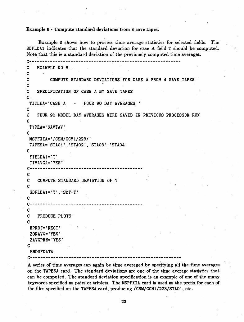
Example 6 - Compute standard deviations from 4 save tapes.

Example 6 shows how to process time average statistics for selected fields. TheSDFLDA1 indicates that the standard deviation for case A field T should be computed.Note that this is a standard deviation of the previously computed time averages.

C--------------------------------------

C EXAMPLE NO 6.CC COMPUTE STANDARD DEVIATIONS FOR CASE A FROM 4 SAVE TAPESCC SPECIFICATION OF CASE A BY SAVE TAPESC

TITLEA='CASE A - FOUR 90 DAY AVERAGESCC FOUR 90 MODEL DAY AVERAGES WERE SAVED IN PREVIOUS PROCESSOR RUNC

TYPEA='SAVTAV'C

MSPFXIA='/CSM/CCM1/223/'TAPESA='STAO1','STAO2','STA03','STA04'

CFIELDA1='T'TIMAVGA='YES'

C----------- __-----------

CC COMPUTE STANDARD DEVIATION OF TC

SDFLDA1='T'.'SDT-T'CC----------------- -----------CC PRODUCE PLOTSC

HPROJ='RECT'ZONAVG='YES'ZAVGPRN='YES'

CENDOFDATA

C--------------___-----------------

A series of time averages can again be time averaged by specifying all the time averageson the TAPESA card. The standard deviations are one of the time average statistics thatcan be computed. The standard deviation specification is an example of one of the manykeywords specified as pairs or triplets. The MSPFXIA card is used as the prefix for each ofthe files specified on the TAPESA card, producing /CSM/CCM1/223/STAO1, etc.

23

Example 7. Produce two five-day time averages and average the results.

Some tasks cannot be completed in one processor jobstep, but the intermediate results

might not need to be saved (except to the Cray disk). In this case, multiple sets of ICP

decks can be combined as shown, to produce the desired result. Also, the parameter G1 in

the JCL must be changed to match the desired number of jobsteps. In this example, the

composite average of two five-day time averages is computed by using 3 jobsteps.

C------------ -- -------------------

C EXAMPLE NO. 7

C

C CREATE TWO FIVE-DAY TIME AVERAGES,

C AND AVERAGE THE RESULTS (3 JOBSTEPS).

C------ ---.---- ---------..... 0..---- ----------- ---------

C JOBSTEP 1. CREATE THE FIRST TIME AVERAGE

C

C TIME AVERAGE FOR MODEL DAYS 6-10

C

TITLEA='TEST RUN - JOBSTEP 1'

MSPFXI= '/CSM/CCM1/223/'

TAPESA='X22301'

DAYSA=6.0,10.5,0.5

FIELDA1='T'

C

TIMAVGA='YES'

C

C CREATE A ZONAL AVERAGE OF THE TIME AVERAGE

C (IT WILL NOT BE PRINTED, SINCE THERE IS NO ZAVGPRN KEYWORD)

C

ZONAVG='YES'

C

C WRITE THE RESULTS OF CASE A TO THE CRAY DISK WITHOUT

C SAVING IT TO THE Mass Store (IT WILL BE AVAILABLE FOR THE

C NEXT JOBSTEP).

C

SAVTAVA='TAPEI','NOMS'

24

C

C DON'T DISPOSE THE PLOTS YET

C

DPLTMF='NO'

C

C NOTE: FIRST ENDOFDATA CARD. BE SURE EACH GROUP OF CARDS

C REPRESENTING A JOBSTEP ENDS WITH AN ENDOFDATA CARD.

C

ENDOFDATA

C- --------------- ----------------------------------------------

C

C JOBSTEP 2. DO SAME OPERATIONS FOR SECOND TIME AVERAGE.

C

TITLEA='TEST RUN - JOBSTEP 2'

MSPFXIA='/CSM/CCM1/240/'

TAPESA='X24001'

TIMAVGA='YES'

C

C TIME AVERAGE FOR MODEL DAYS 6-10

C

DAYSA=6.0,10.5.0.5

FIELDA1='T'

C

C CREATE A ZONAL AVERAGE OF THE TIME AVERAGE

C (IT WILL NOT BE PRINTED, SINCE THERE IS NO ZAVGPRN KEYWORD)

C

ZONAVG='YES'

C

SAVTAVA='TAPE2','NOMS'

C

C DON'T DISPOSE THE PLOTS YET

C

DPLTMF='NO'

C

ENDOFDATA

C---- -------- -----------

25

cC JOBSTEP 3. TIME AVERAGE OF THE TWO SAVE TAPES.

CTAPESA='TAPE1','TAPE2'TYPEA='SAVTAV'FIELDA1='T'TIMAVGA='YES'ENSMBLA='CASE'

CC CREATE A ZONAL AVERAGE OF THE COMPOSITE TIME AVERAGE

C (IT WILL BE PRINTED THIS TIME).CZONAVG='YES'ZAVGPRN='YES'

CENDOFDATA

C----------------------------------- ---------------

Example 7 demonstrates that a more complicated task can be built from a series of simplejobsteps. Each of the first twojobsteps creates a time average. The third jobstep computesthe time average of the first two. The EMSMBLA keyword specifies emsemble averaging ofthe tapes TAPE1 and TAPE2, when it is set to the value CASE. This option allows averagingof multiple tapes with the same time values. Here, the two tapes are averaged over thesame time period, so that the average of the two tapes is an average of the two cases.

Where to find other examples.

The complete Processor Users' Guide (Wolski, 1987) contains samples of plots (Ap-pendix A) and a listing of the neccesary ICPs to generate these groups. These examplesmay also serve as an aid to constructing ICP decks for certain purposes.

26

3.3 A Brief List of Processor Options

The following is a summary of some of the available keywords for each 'category' ofprocessor function. Case dependent ICPs have a 'c' suffix, with the cases for which it isvalid listed in parentheses. The 'n' suffix indicates a field-pass dependent keyword. Referto the Processor User's Guide for a complete description of the purpose and use of eachkeyword.

There are four major divsions of the ICPs for the following tables. These four divisionsare further divided by processing function. These categories are:

* DATA INPUT OPTIONS* Input Data Specification* LSD Driver* Input Data Modification* History Tape Input Data Limiting* Mass Store File Input* User Defined Derived Fields

* PROCESSING OPTIONS* Case Comparison/Merging* Color Plotting* Horizontal Plotting* Spatial Averaging* Spectral Processing* Time Average Statistics* Time Average Zonal Statistics* Time Filtering* Time Series Plots* Vertical Cross-Section Plotting

* DATA OUTPUT OPTIONS* Field Value Printing* Plot Disposition* Mass Store File Output* Save Tape Production

* MISCELLANEOUS OPTIONS* Dataset Management* Memory Management* Miscellaneous Plotting

For each specific category listed above, in order, there follows a table of the keywordname, possibly with a 'c' or 'n' suffix (see above), a brief description of the purpose of thekeyword, and an example of its use. Keywords new to this version of the processor areindicated by a superscripted asterisk (e.g. KEYWORD*) in the Option column for thatkeyword. The (A,B) under purpose indicates the keyword is valid for cases A and B only.

27

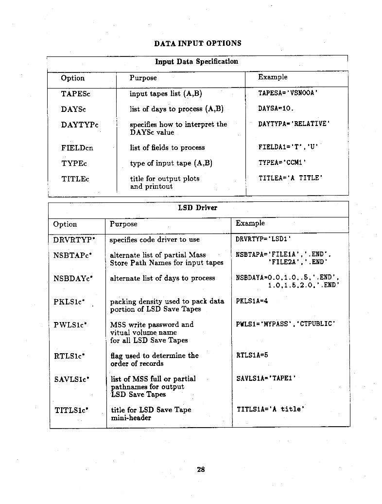
DATA INPUT OPTIONS

Input Data Specification

Option Purpose Example

TAPESc input tapes list (A,B) TAPESA='VSNOOA'

DAYSc list of days to process (A,B) DAYSA=10.

DAYTYPc specifies how to interpret the DAYTYPA='RELATIVE'DAYSc value

FIELDcn list of fields to process FIELDA1=T'. 'U'

TYPEc type of input tape (A,B) TYPEA='CCM1'

TITLEc title for output plots TITLEA='A TITLE'and printout

LSD Driver


DRVRTYP* specifies code driver to use DRVRTYP='LSD1'

NSBTAPc* alternate list of partial Mass NSBTAPA='FILE1A',' .END',Store Path Names for input tapes 'FILE2A','.END'

NSBDAYc* alternate list of days to process NSBDAYA=0.0,1.0,.5,'.END',1.0.1.5,2.0,'.END'

PKLSlc* packing density used to pack data PKLS1A=4portion of LSD Save Tapes

PWLSlc* MSS write password and PWLS1='MYPASS' 'CTPUBLIC'vitual volume namefor all LSD Save Tapes

RTLSlc* flag used to determine the RTLS1A=5order of records

SAVLSlc* list of MSS full or partial SAVLS1A='TAPEl'pathnames for outputLSD Save Tapes

TITLSlc* title for LSD Save Tape TITLS1A='A title'mini-header

28

Input Data Modification


ENSMBLc option to process as an ensemble ENSMBLA='CASE'the same day from multipleinput tapes (A,B)

MASKSc mask the input data according MASKSA='LAND','SICE'to the surface type flags (A,B)

TIMAVGc option to time average input (A,B) TIMAVGA= 'YES'

Vertical interpolation to pressure surfaces

INTDP set default interpolation type code INTDP=2

LBTDP default lower boundary treatment code LBTDP=4

NLCDP default number of planetary boundary NLCDP=0layer levels to copy

PINTXL interpolation exceptions list PINTXL='HT1'.2,1.0

PRESSLE pressure surfaces to interpolate to PRESSLE=1000.,850.,700.....

Vertical interpolation to potential temperature surfaces

INTDT* set default interpolation type code INTDT=2

LBTDT* default lower boundary treatment code LBTDT=4

NLCDT* default number of planetary boundary NLCDT=Olayer levels to copy

TINTMLT* flag to indicate how multiple occurences TINTMLT='BLOCK'of a given potential temperaturesurface are handled

TINTXL* interpolation exceptions list TINTXL='HT1',2.1.0

TEMPLEV* analogous to PRESSLE except that TEMPLEV=300..list is potential temperature surfaces 280. ,260.....in degrees K

29

History Tape Input Data Limiting

Mass Store File Input


MSPFXI* case-independent Mass Store Path MSPFXI='/CSM/CCM1/999/'Name prefix for input datasets

MSPFXIc* case-dependent Mass Store Path MSPFXIA = ' /CSM/CCM1/999/'Name prefix for input datasets

MSTXTI* case-independent text string for MSTXTI=20HKEYWORD='value'Mass Store input datasets

MSTSTIc* case-dependent text string for MSTXTIA=20HKEYWORD= 'value'Mass Store input datasets

PDNIDI* case-independent ID to use on PDNIDI='PDNID'ACQUIRE for input datasets

PDNIDIc* case-dependent ID to use on PDNIDIA='PDNID'ACQUIRE for input datasets

User Defined Derived Fields


DERFLD define a new field DERFLD='TCELS' .61.2.3.0.'T',273.15 ,:MINUS', 'END'

FLDSRCc determines how two resolve FLDSRC='INPUT'ambigutites if the derived fieldname conflicts with an inputfield name (A,B)

30


DEFLDcn* explicit field deletion list DEFLDA1='T',61

SIGLEVc option to limit the sigma SIGLEVA=1.4,5levels processed (A,B)

SURFLEV option to exclude the surface level SURFLEV= 'NO'

SUBPc option to limit input pressure levels (A,B) SUBPA=1,4,5I

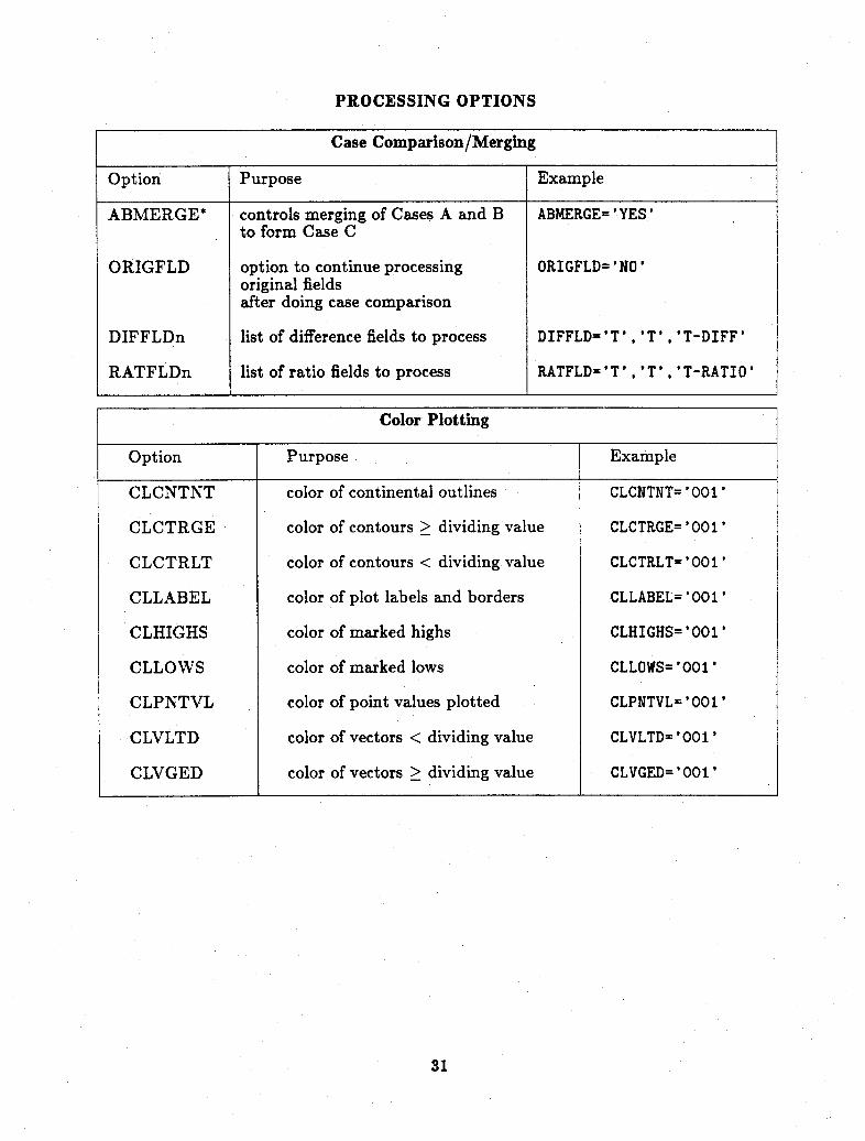
PROCESSING OPTIONS

Case Comparison/Merging

31


ABMERGE* controls merging of Cases A and B ABMERGE= 'YES'to form Case C

ORIGFLD option to continue processing ORIGFLD='NO'original fieldsafter doing case comparison

DIFFLDn list of difference fields to process DIFFLD='T' 'T'. 'T-DIFF'

RATFLDn list of ratio fields to process RATFLD='T'. 'T' 'T-RATIO'

Color Plotting


CLCNTNT color of continental outlines CLCNTNT='001'

CLCTRGE color of contours > dividing value CLCTRGE='001'

CLCTRLT color of contours < dividing value CLCTRLT='001'

CLLABEL color of plot labels and borders CLLABEL='001'

CLHIGHS color of marked highs CLHIGHS= '001'

CLLOWS color of marked lows CLLOWS='001'

CLPNTVL color of point values plotted CLPNTVL='001'

CLVLTD color of vectors < dividing value CLVLTD='001'

CLVGED color of vectors > dividing value CLVGED='001'

Horizontal Plotting


HPROJ horizontal plot projection HPROJ='POLAR'specification

HEMIS hemisphere plot option if HEMIS='NORTH'HPROJ='POLAR'

HPCINT contour interval specification for HPCINT= 'T', 500., 10.horizontal plots

DASHLIN option to dash some contours DASHLIN='YES'

HPCDIV contour dividing value (either for HPCDIV= T',500.,240.dashed or 2-color plots)

HPPTVAL option to print values on HPPTVAL='BOTH'horizontal plots instead of orin addition to contour plots

HPSCAL scale factor for plot contour labels HPSCAL='T',500.,100.

HPLFPVn field pairs to be plotted as vectors HPLFPV1='U' 'V', 'WIND'

HPVOPT vector plot option for the HPLFPVn HPVOPT='VECT'HPLFPVn keyword

HPVSCAL scale factor for horizontal plots HPVSCAL='WIND ',500.,20.

HPVDIN vector density plotting increment HPVDIN=1

HPVDIV vector dividing value (colors only) HPVDIV='U','V,'WIND'

Limited Area Horizontal Plots

HPRBNDS* boundaries for horizontal HPRBNDS=-180.,60.,10. 90.rectangular plots

HPRNDIV* number of plot divisions (halvings) HPRNDIV=2for horizontal rectangular plots

32

I I

Spatial Averaging


MERAVG meridional averaging option MERAVG='YES'

MAVGDSP* disposition of meridional average data MAVGDSP='PLTPROC'

MAVGPRN option to print meridional averages MAVGPRN='YES'

MAVRNG range of latitudes for meridional average MAVRNG=-45. ,45.

MBKFR blocking fraction for valid meridional avg. MBKFR=.1

VERAVG vertical averaging option VERAVG='YES'

VAVGDSP* disposition of vertical average data VAVGDSP='PROC'

VAVRNG vertical averaging range VAVRNG=1000.,600.

VBKFR blocking fraction for valid vertical avg. VBKFR=.01

ZONAVG zonal averaging option ZONAVG='YES'

ZAVGDSP* disposition of zonal average data ZAVGDSP='PLTPROC'

ZAVGPRN option to print zonal averages ZAVGPRN='YES'

ZAVRNG range of longitudes for zonal average ZAVRNG=-145.,145.

ZBKFR blocking fraction for valid zonal average ZBKFR=.1

MSKFLcn masked area average specification (A,B) MSKFLA1='T','TM','LAND','OCEAN',15.,75.,-135.,60.

MSKAP determines if ordinary MSKAP='NO'masked area averages are computed

MSKAPS determines if the masked area MSKAPS='NO'average of the squares is computed

MSKAZS option to compute the masked area MSKAZS='NO'average of squares of zonal averages

SFCTTAP name of surface type save tape to read SFCTTAP='SR15JA'

SFCTCRT name of surface type save tape to create SFCTCRT='SR15JA'

33

I

Spectral Processing

34


SPCINTc changes horizontal resolution(A,B) SPCINTA=15,15.30,50.40

SPCMNKc* spectral transformation parameters SPCMNKA=15,15,30to use when transforming gridpointdata into spectral space

SPSNGRF controls spectral graphics SPSNGRF='YES'

SPGYINT controls y-interval range on SPGYINT=1.E4spectral graphs

SPCcn controls spectral processing(A,B) SPCA1='YES'

SPCBPcn sets range of spectral SPCBPA1=0,5.1.6bandpassing(A,B)

SPCDFcn indicates fields to be deleted before SPCDFA1='T','Q'return to grid-point space(A,B)

SPCEFcn fields to be excluded from SPCEFAi='T'spectral processing(A,B)

SPCVP defines fields as vector pairs for SPCVP='TAUX','TAUY'.purpose of computing vector pair 'DIV-TAU','VOR-TAU',derived fields in spectral space 'CHI-TAU' 'PSI-TAU',

'UD-TAU' 'UZ-TAU','VD-TAU','VZ-TAU'

Time Average Statistics


CVFLDcn list of covariance fields CVFLDA1='U' 'V', 'UV-COVR'to compute (A,B)

SDFLDcn list of standard deviation fields SDFLDA1='T'. 'STD-T'to compute (A,B)

TCFLDcn list of total eddy covariance fields TCFLDA1='U' ,'V','TCVR-UV'to compute (A,B)

PRFLDcn list of product fields PRFLDAI='U'. 'V', 'PROD-UV'to compute (A,B)

Time Average Zonal Statistics

35


ZSTFLcn time average zonal standard ZSTFLA1='T', 'T-ZSDV'deviations (A,B)

ZCVFLcn time average zonal ZCVFLA1='U' 'V', T-CVFL'covariances (A,B)

Time Filtering


TIMFILc time filtering option (A,B) TIMFLA='LOWP'

TFWTSc array of filtering weights to use (A,B) TFWTSA=-1., 1.

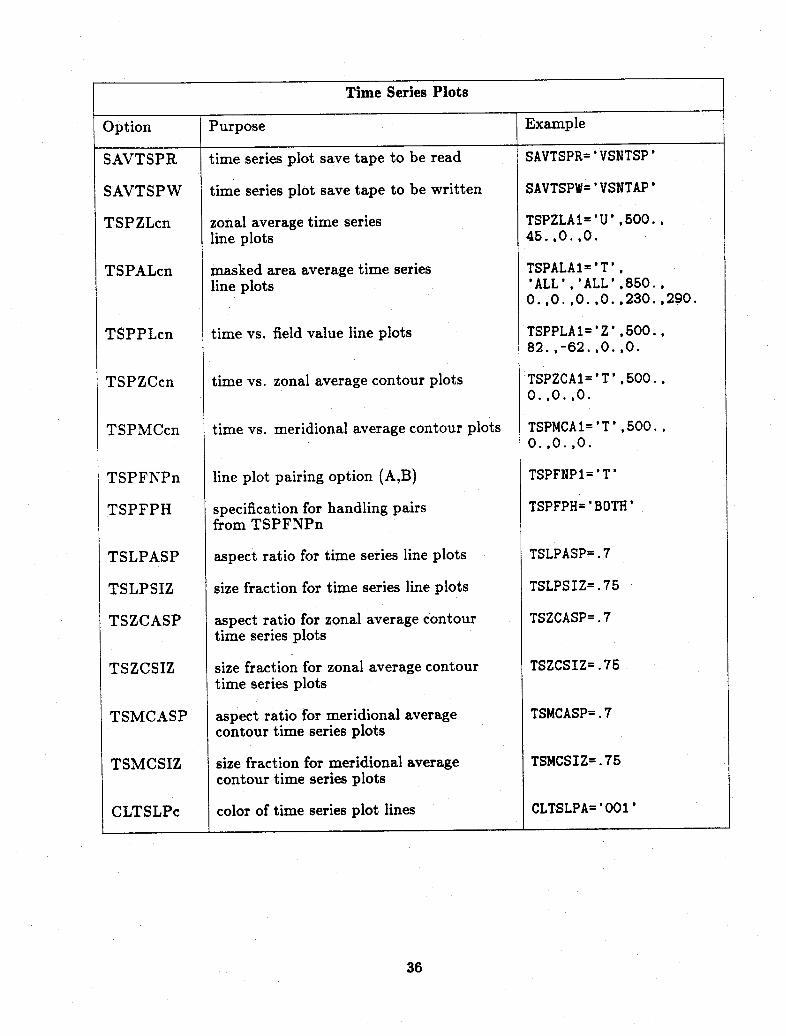
Time Series Plots

Option Purpose

SAVTSPR

SAVTSPW

TSPZLcn

TSPALcn

TSPPLcn

TSPZCcn

TSPMCcn

TSPFNPn

TSPFPH

TSLPASP

TSLPSIZ

TSZCASP

TSZCSIZ

TSMCASP

TSMCSIZ

CLTSLPc

time series plot save tape to be read

time series plot save tape to be written

zonal average time seriesline plots

masked area average time seriesline plots

time vs. field value line plots

time vs. zonal average contour plots

time vs. meridional average contour plots

line plot pairing option (A,B)

specification for handling pairsfrom TSPFNPn

aspect ratio for time series line plots

size fraction for time series line plots

aspect ratio for zonal average contourtime series plots

size fraction for zonal average contourtime series plots

aspect ratio for meridional averagecontour time series plots

size fraction for meridional averagecontour time series plots

color of time series plot lines

Example

SAVTSPR='VSNTSP'

SAVTSPW='VSNTAP'

TSPZLA1='U',500.,45.,0.,0.

TSPALA1='T','ALL','ALL',850.,0.,0.,0.,0.,230.,290.

TSPPLA1='Z',500.,82.,-62.,0.,0.

TSPZCA1='T',500.,0. 0. ,0.

TSPMCA1='T',500.,0. 0. 0.

TSPFNP1='T'

TSPFPH='BOTH'

TSLPASP=.7

TSLPSIZ=.75

TSZCASP=.7

TSZCSIZ=.75

TSMCASP=.7

TSMCSIZ=.75

CLTSLPA='001'

36

-

i I

I II

.

k

I

Vertical Cross-Section Plotting

Option

LMLFPSL

LXASPRT

LXCINT

LXCDIV

LXLNSCL

LXSCAL

LXSIZE

LXPTVAL

MXASPRT

MXCDIV

MXCINT

MXLNSCL

MXLTRNG

MXSCAL

MXSIZE

MXPTVAL

MXPLOT

LXPLOT

ZORD

Purpose

list of multilevel fields to plot assingle levels

lat. x-section plot aspect ratio

latitudinal x-section plot contour interval

lat. x-section plot dividing value

lat. x-section plot logarithmic scale option

lat. x-section plot scale factor

lat. x-section plot fractional size

option to print point values onlatitudinal x-section plots

aspect ratio of meridional x-section plot

meridional x-section plot contourinterval dividing value

meridional x-section plot contour interval

meridional x-section plot logarithmicscale option

lat. range for meridional cross-section plots

meridional x-section plot scale factor

fractional size of meridional x-section plot

option to print point values on meridionalx-section plots

option to explicitly plot all availablemeridional cross-sections

option to explicitly plot all availablelatitudinal cross-sections

controls the addition of a height scale on allvertical cross-section plots

Example

LMLFPSL='T'

LXASPRT=.7

LXCINT='T',10.

LXCDIV='T',240.

LXLNSCL='YES'

LXSCAL='U',100.

LXSIZE=.75

LXPTVAL='BOTH'

MXASPRT=.7

MXCDIV='T',240.

MXCINT='U',100.

MXLNSCL='YES'

MXLTRNG=-90.,90.

MXSCAL='Q',1.E8

MXSIZE=.75

MXPTVAL='BOTH'

MXPLOT='YES'

LXPLOT='YES'

ZORD='YES'

37

---- --

--

DATA OUTPUT OPTIONS

38

Field Value Printing


PRINTc field printing switch PRINTA='YES'

PRFNMc list of fields to print PRFNMA='T'

PRLATc list of latitudes to print PRLATA=O.,10.

PRLONc list of longitudes to print PRLONA=-60.,170.

PRLEVc list of levels to print PRLEVA=850.,500.

PRLIMR limiting range of values for printing PRLIMR=280.,300.

NSDPRNT number of significant digits NSDPRNT=8to compare for case comparison

Plot Disposition Options


DPLTCA Specifies Dicomed camera to use for each DPLTCA='FICHE'corresponding value of DPLTMF

DPLTCT Specifies default processor case title to use DPLTCT='A'for dicomed plot title

DPLTFN File name to use for dispose of a plot file DPLTFN='PLOTS'

DPLTFT File type to use for dispose of a plot file DPLTFT='METACODE'(IBM 4381 only).

DPLTIT Dicomed output plot title DPLTIT='Test Title'

DPLTMF Name(s) of NCAR Local Network node for DPLTMF='Dl', 'I0'plot disposition

DPLTXT* character string to append to text DPLTXT='USER=OTHER'field for plot file DISPOSE

MNFRMS minimum number of frames produced per MNFRMS=10000dispose group

MXFRMS maximum number of frames produced per MXFRMS= 10000dispose group

39

Mass Store File Output


MSPFXO* case-independent Mass Store Path MSPFXO='/MYNAME/SAVTAV/'Name for output datasets

MSPFXOc* case-dependent Mass Store Path MSPFXOA='/MYNAME/SAVTAV/'Name for output datasets

MSTXTO* case-independent text string for MSTXTO=20HKEYWORD='value'Mass Store output datasets

MSTXTOc* case-dependent text string for MSTXTOA=20HKEYWORD='value'Mass Store output datasets

MSRTO* case-independent Mass Store dataset MSRTO='365'Retention Time

MSRTOc* case-dependent Mass Store dataset MSRTOA='365'Retention Time

PDNIDO* case-independent ID to use on SAVE PDNIDO='PDNID'for output datasets

PDNIDOc* case-dependent ID to use on SAVE PDNIDOA='PDNID'for output datasets

Save Tape Production


BPHSTc option to write history tape when BPHSTA='YES'there are blocked points

OFTHSTc* format for output history tapes OFTHSTA='CCM1'

PKHSTc packing density for output PKHSTA=1history save tapes (A,B)

PWDHSTc write password, and Mass Store PWDHSTA='PASSWD'virtual volume for all history save tapes

NDYHSTc maximum number of days to put NDYHSTA=30on a single history tape (A,B)

SAVMHST* mode flag for output History SAVMHST='TAV'Save Tapes

SAVTAVc Output time average save tape SAVTAVA='VSNOO1'Specification

SAVTSRc Output time series save tape list SAVTSRA='VSNTSR'

NDYTSRc maximum number of days for each NDYTSRA=60time series tape

PWDTSRc write password for time PWDTSRA='MYPASS'series tapes

SAVMTSR* mode flag for output of Time Series SAVMTSR='TAV'Save Tapes

SAVHSLc specification for horizontal slice SAVHSLA='VSNHSL'save tape

SHSLZAV option to put zonal average values SHSLZAV='YES'on the horiz. slice save tape

SAVMHSL* mode flag for output horizontal SAVMHSL='TAV'slice Save Tapes

40

I

MISCELLANEOUS OPTIONS

Dataset Management Options

Memory Management Options


MEMORY no. of words of memory to pre-allocate MEMORY=200000

MEMCON memory conservation option MEMCON='YES'

Miscellaneous Plotting Options


INDEX controls production of the plot index INDEX='PRINT'

NUMPLT controls whether or not a frame number NUMPLT= 'YES'is printed at the bottom of each plot

PTOPc pressure at the top of the model, used for PTOPA=O.computing code-defined derived field DELPRES

41


DELREL controls disposition of input permanent DELREL=1datasets once they have been read

DELPDN list of permanent disk datasets to delete DELPDN='VSNOO1'

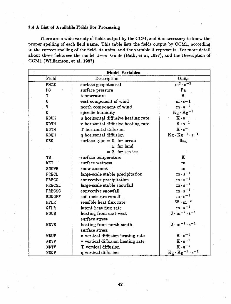
3.4 A List of Available Fields For Processing

There are a wide variety of fields output by the CCM, and it is necessary to know theproper spelling of each field name. This table lists the fields output by CCM1, accordingto the correct spelling of the field, its units, and the variable it represents. For more detailabout these fields see the model Users' Guide (Bath, et al, 1987), and the Description ofCCM1 (Williamson, et al, 1987).

Model VariablesDescription

surface geopotentialsurface pressuretemperatureeast component of windnorth component of windspecific humidityu horizontal diffusive heating ratev horizontal diffusive heating rateT horizontal diffusionq horizontal diffusionsurface type = 0. for ocean

= 1. for land= 2. for sea ice

surface temperaturesurface wetnesssnow amountlarge-scale stable precipitationconvective precipitationlarge-scale stable snowfallconvective snowfallsoil moisture runoffsensible heat flux ratelatent heat flux rateheating from east-westsurface stressheating from north-southsurface stressu vertical diffusion heating ratev vertical diffusion heating rateT vertical diffusionq vertical diffusion

UnitsI

m 2 .- 2

PaK

m-s-lm*s-1m-s

Kg Kg-1K.s- 1

K.s- 1

K.s-1

Kg-Kg- 1 s-flag

Kmm

-1m-s

*-1m.s~

MS-1m.s-1m-s

W.m- 2

J.m-2 S- 1

J-m-2.s-1

K.s-1K.s-1K.s-1

Kg.-Kg- 1 s- 1

42

FieldPHISPSTUV

QNDUHNDVHNDTHNDQHORO

TS

WETSNOWHPRECLPRECCPRECSLPRECSCRUNOFFHFLR

QFLRNDUS

NDVS

NDUVNDVVNDTV

NDQVii _ l----

Model Variables (cont'd)Description

average net downward solar fluxat surfaceaverage net downward longwaveflux at surfaceaverage net longwave flux at topof modelaverage absorbed solar fluxaverage planetary albedo at topof atmospherefractional cloud covercloud emissivityclear sky longwave flux at topclear sky solar flux at topclear sky longwave flux atsurfaceclear sky solar flux at surfaceomega vertical velocitytotal condensation rateeast-west surface stressnorth-south surface stressnet downward radiation fluxesshort wave heating ratelong wave heating ratesolar insulationu tendencyv tendencyT tendencyq tendencysurface pressure tendencychange in T from convectiveadjustmentschange in q from convectiveadjustments

Units

W.m-2

W.m- 2

fraction

fractionfractionW.m-2W em-2

W.m-2

W.m-2

Pa.s- 1

kg m- 2 .s- 1

N m-2N.m-2W.m-2K.s-1

K.s- 1

W .m-2m.s-2

-2m-s

K.s- 1

Kg Kg-1 s- 1

Pa.s- 1

K.s-1

Kg - Kg- . s- 1

43

FieldFRSA

FRLA

FIRTP.

SABTPALBT

CLOUDCLOUDECLRLTCLRSTCLRLS

CLRSSOMEGA

QCTAUXTAUYSRADQRSQRLSOLINUTENDVTENDTTEND

QTENDLPSTENDTCOND

DQCOND

--%

I-

Additionally, many derived fields are available. These fields are requested in the samemanner as fields output directly from the model. These are the derived fields currentlyavailable from the processor when processing CCM1 history tapes:

Processor Derived VariablesDescription

velocity potentialcondensational heating ratepressure layer thicknesshorizontal wind divergencekinetic energy of differencesx-derivative of natural log of surface pressurey-derivative of natural log of surface pressurevelocity magnitude of differencesnet total atmospheric energy fluxnet surface energy fluxnet top of Model energy fluxgeopotential height, full levels,CCMOB formulationgeopotential height, full levels,CCM1 formulationkinetic energykappa*temperature*omega/pressure,CCMOB versionkappa*temperature*omega/pressure,CCM1 versionnatural log of surface pressurewater vapor mass (3-dimensional)net energy flux into surfacetotal precipitationpressure on sigma surfacesstream functionsea-level pressuremoisture source termnet radiation (same as RAD, withdifferent units)relative humiditysigma vertical velocity at full Model levelssigma vertical velocity at half Model levelstotal cloud fraction3-D sinusoidal test field

Unitsm 2 -

K.dy- 1

Pas-1

J kg- 1

Pa.m- 1

Pa.m- 1

-- 1

W.m-2

W.m-2

m

m

2 -2

K s- 1

en(Pa)Kg m-2

W-m-2mPa

m 2 .s-1

PaKg m- 2

K.dy- 1

fractions-1s-1

fraction

44

FieldCHICONDHDELPRESDIVDKEDLNPSXDLNPSYDVMAGENETENETSENETTHTO

HT1

KEKTOOPVO

KTOOPV1

LNPS

MQNRADSPRECTPRESPSIPSL

QSRCRADD

RELHUMSIGDOTFSIGDOTHTCLDTEST

. . II III-----

Processor Derived Variables (cont'd)Description

potential temperature on sigma surfacestemperature modified for use incomputing KTOOPV1water vapor mass in a column (2-dimensional)virtual temperatureu-velocity computed from divergence alonetotal kinetic energy spectrakinetic energy spectra (divergent part)kinetic energy spectra (rotational part)u-velocity computed from vorticity alonevertical advection of generic field VADGINvertical advection of temperature,CCMOB versionvertical advection of temperature,CCM1 versionvertical advection of Q, CCMOB versionvertical advection of Q, CCM1 versionvertical advection of U, CCM1 versionvertical advection of V, CCM1 versionkinetic energy variancev-velocity computed from divergence alonevertical integral of kinetic energyvertical integral of potential energyvertical integral of total energymagnitude of horizontal windhorizontal wind vorticityv-velocity computed from vorticity alonegeopotential height

UnitsKK

Kg. m- 2

Km-s

J. Kg-J Kg- 1

J. Kg- 1

ms - 1

VADGINt s-1K.s-1

K.s-1

Kg · Kg- 1 · s-Kg- Kg-l s- 1

m -2

m* -2

m * s-1J * m- 2

Jm-2

J m-2

s- 1

m- - 1

m

-1 ·

t The units of this variable are the units of field VADGIN per second.

You should consult the Processor User's Guide before requesting any derived fields.It is necessary to understand when each field is derived, and most derived fields are notavailable when processing save tapes. Other derived fields can either be produced by somecode modification on your part, or by the use of user-defined derived fields.

45

FieldTHETATMODK

TMQTVUDUVSQUVSQDUVSQRUZVADVGV1VADVTVO

VADVTV1

VADVQVOVADVQV1VADVUVIVADVVV1VARWVVDVIKEVIPE

VITEVMAGVORVZZ

.

- Ir-

I I --

3.5 User-defined Derived Fields

The ability to create user-defined derived fields is shown by example in Section 3.3(keyword DERFLD). User-defined keywords are defined using a series of operators in ReversePolish Notation. The example of:

DERFLD='TCELS' ,61,2,3,0,'T',273.15,'.MINUS ','.END'

is an example converting temperature from degrees Kelvin to degrees Celsius. The firstparameter is the name of the derived field ('TCELS'), the second parameter indicates whenthe computation should be done in the code (61 - before vertical averaging (after timeaveraging)), the third parameter is the vertical placement flag (2 - multilevel fields locatedat layer midpoints), the fourth is the vertical coordinate flag (3 - can compute if data is onsigma or pressure surfaces), the fifth is the spectral parity flag (0 - parity not applicable),the 273.15 is a scalar value to be applied to the field 'T', and the ':MINUS' is the operatorto be applied. Each group defining a derived field ends with the '.END' parameter. Theresult of the above expression is to subtract 273.15 from all values of the 'T' field. Thisprovides you with a capability to define fields in terms of other fields without modifying theprocessor code. The operators available apply either to a single value (Unary Functions)or to two values (Binary Functions). They are listed in the following tables.

Function.END.CONST.MINUS.ABS.SQRT.ALOG.ALOG10.EXP.VSUM.DSWVSUM.DSTIMES.SHIFTUP.SHIFTDN.TSINL.TCOSL.ZAVDEV.LEVELnn

Descriptionexpression and definition group terminatorcreate a constant-value multilevel fieldnegate operandabsolute valuesquare rootnatural logarithmcommon (base 10) logarithme ** operandvertical sum of all levelsdelta sigma weighted vertical sum of all levelsdelta sigma times each levelshift field upward by one levelshift field downward by one levelmultiply operand by sine of latitudemultiply operand by cosine of latitudereplace operand by deviations from zonal averageextract level nn (counting from bottom)(result is the single, extracted level)

46

Unary FunctionsI

_

I I I

A complete description of this capability is given in the complete Users' Guide. Pleaserefer to this document for more detailed information about this capability, including otherexamples of the use of the 'DERFLD' keyword.

47

Binary FunctionsOP1 is the leftmost operand, OP2 the rightmost.

At least one operand must be a field,unless otherwise noted.

Function Description:PLUS OP1 + OP2:MINUS OP1- OP2:TIMES OP1 * OP2:DIVIDE OP1 / OP2:MIN minimum(OP1,OP2):MAX maximum(OPi,OP2):POWER OP1 ** OP2:AMOD mod(OP1,OP2):L1TIMES OPl*(bottom level of OP2) (two fields only):EQ .T. iff OP1.EQ.OP2:NE .T. iff OP1.NE.OP2:LT .T. iff OP1.LT.OP2:GT .T. iff OP1.GT.OP2:LE .T. iff OP1.LE.OP2:GE .T. iff OP1.GE.OP2:AND .T. iff OP1.AND.OP2 (two fields only):OR .T. iff OP1.OR.OP2 (two fields only):LEVMASK mask field to 0. at certain levels:UNBLOCK field OP1 blocked points take values of corrseponding

points at OP2

3.6 Accessing the Online Documentation

Detailed documentation for the Modular Processor is available in two forms. An'online' version is available to users on the IBM 4381. A printed version of the samedocumentation is also available (Wolski, 1987). The two forms of documentation can beused together to quickly find information about specific aspects of the processor.

An IBM command procedure called PROCDOC is used to view the file. A help file hasbeen provided to provide instructions on accessing the documentation.

To access the online documentation help file, you must enter:

LINKTO CSMLIB <CR>

and the system will respond with:

*** CSMLIB'S 191-DISK LINKED AS DASD nnn WITH FILEMODE m ***

where nnn is the device number assigned and m is the filemode, or subdirectory associatedwith the CSMLIB's files.

you then enter the command:

HELP PROCDOC

From this point, the instructions will lead to the online documentation. Instructions within

the online documentation will show you how to utilize and efficiently use the documenta-tion. You are encouraged to select an example from section 3.2 and read the definitions ofsome of the ICPs in the example selected.

48

4.0 Processor Output

There are at least three output files produced by the processor for most jobs. Thefirst is a printed summary of processing done and the total number of plot frames produced.The second is the plot file, which can then be disposed of by whatever method is mostconvienient for the user. The third is the save tape output file produced from the run.

Following the description of the printed and graphical output is a sample run createdfrom the ICP deck shown in section 2.

4.1 Graphical Output

There are several options for plot file disposition. The keywords DPLTCA, DPLTCT,DPLTFN, DPLTFT, DPLTMF, and DPLTMF control disposition of the plot file to one or moredestinations for a single jobstep. By default, DPLTFT='D1', so that the plots from eachjobstep are automatically disposed to microfiche. For example, to send plots to the IBM4381 as file GENDECK PLOTS, these cards would be used:

DPLTMF='IO'DPLTFN='GENDECK'DPLTFT='PLOTS'

The file can be sent to the IBM 4381, the NCAR/AAP Vax system, the Dicomed microficheunit, the Dicomed 35mm roll film unit, the Mass Store, or any other NCAR Local Networknode. At the end of the sample printout which follows are a few plots generated from therun whose output is shown in Figure 2.

4.2 Printed Output

The printed output file will automatically be sent to your virtual reader on the IBM4381 unless you change the JCL. This file can be examined or printed in the reader, orloaded to your A disk (type HELP RDRX for more information).

The following illustrates the type of output you should expect to see from a processorrun. The ICPs are echoed to the output file, as well as the plot file. The list of daysprocessed and the processing done are all printed. If no errors are encountered, a messageindicating normal termination and the number of plot frames produced is printed. Theindex of the plot frames generated is also printed. The log file should also be checkedto ensure the correct disposition of the plot file. If any error is encountered, examine theoutput lines just above the beginning of the symbolic debug dump for a processor-producederror message (in the case of a fatal error - the processor also detects and flags non-fatalerrors). This will often save a great amount of time, since many errors are flagged by theprocessor, and the ABORT is called internally to prevent wasted processing.

49

4.3 Save Tape Output

The save tape output is produced whenever you use one of the 'SAV. .. ' keywords.There are a large number of options for specifying where and how that dataset will besaved. In order to properly specify save tape output, you must specify keywords from twogroups:

* save tape keywords,

* Mass Store output keywords.

These two groups contain most of the keywords you will need to write save tapes. Anexample of using keywords from these two groups is:

SAVTAVA = 'FILEI'

MSPFXOA = '/SMITH/SUBDIR/'

This will save file /SMITH/SUBDIR/FILE1 on the Mass Store.

50

*** INPUT CONTROL PARAMETERS FOR OBSTEP 1 **CC INPUT CONTROL PARAMETERS - JOB STEP 1CC INPUT SPECIFICATIONSC

TITLEA a 'PROC02 TEST RUN'TAPESA * 'X22301'MSPFXI a '/CSM/CCM1/223/'DAYSA 5.FIELOA1 'T'

CC DATA MANIPULATION SPECIFICATIONSC

PRESSLEV - 900..800. ,700..500. .400. .200. 200. 100.CC PLOT SPECIFICATIONSC

HPROdJ 'RECT'ZONAVG - 'YES'ZAVGPRN * 'YES'

CC PLOT OUTPUT SPECIFICATIONSC

DPLTMF * '10'DPLTFN * 'SAMPLE'DPLTFT a 'PLOTS'

CENDOFDATA

ACQUIRING NEXT INPUT DATASET: DN LN01 ; PON MCCM1223X22301 ; ID * CSMTEXT * FLNMs/CSM/CCM1/223/X22301

DAY 5.0000 READ FROM CASE A HISTORY TAPE /CSM/CC1M/223/X22301

** SGUA **

1 1. 00000 1.000002 0.95850 0.991003 0.86850 0.926004 0.73750 0.811005 0.58200 0. 664006 0.42750 0.500007 0.30000 0.355008 0.20500 0.245009 0.13750 0.16500

10 0.08500 . 1100011 0.04250 0.0600012 0 01700 0.0250013 0. 0000 0.00900

** DSIG ***

0.04150000 0.09000000 0.13100000 0.15550000 O.15450000 0.12750000 0.09500000 0.06750000 0.05250000 0.04250000

0.02550000 0.01700000

VARIABLE LOCATION WITHIN TYPE OF LOWER BOUNDARYLAYER INTERPOLATION TREATMENT

T MIDPOINT LOG NO SURF.NO EXTRP

VERTICAL INTERPOLATION COMPLETED FOR CASE A

HORIZONTAL PROJECTION PLOTTING COMPLETED

Fig. 2a. Printout from the generic run deck. The list of input requests is echoed to theoutput, and a message is printed for the day read from the history tape, and thesigma levels on this tape. Messages indicating that the vertical interpolation topressure surfaces and horizontal cross-section plotting have been completed areprinted.

51

ZONAL AVERAGES FOR CASE A: PROC02 TEST RUNCASE ID: 223 CCM1 - CASE223 - JANUARY - 12 LAYERSFIELD: T DAY: 5.0000 LONGITUDE RANGE: -180.0 TO 172.5

LATITUDE 900.OP 800.OP

86.682.277.873.368.964.460.055.551. 146.742.237.833.328.924.420.015.611.16.72.2

-2.2-6.7

-11.1-15.6-20.0-24.4-28.9-33.3-37.8-42.2-46.7-51.1-55.5-60.0-64.4-68.9-73.3-77.8-82.2-86.6

2.6043E+022.5907E+022.5920E+022.5893E+022.5906E+022.6064E+022.6112E+022.6137E+022.6244E+022.6678E+022.7138E+022.7426E+022.7734E+022.8029E+022.8344E+022.8608E+022.8825E+022.8965E+022 .9061E+022.9109E+022.9150E+022.9174E+022.9147E+022.9096E+022.8992E+022.8875E+022.8696E+022.8480E+022.8243E+022.8020E+022.7813E+022.7617E+022.7457E+022.7294E+022.7118E+021.OOOOE+361.OOOOE+361.0000E+361.OOOOE+361.OOOOE+36

700.OP 600.GO SQO0OP 400.OP 300.0P 200.OP

2.5626E+02 2.4801E+022.5651E+02 2.4957E+022.5639E+02 2.5154E+022.5713E+02 2.5306E+022.5753E+02 2.5353E+022.5813E+02 2.5319E+022.5874E+02 2.5297E+022.5893E+02 2.5335E+022.5964E+02 2.5441E+022.6150E+02 2.5614E+022.6472E+02 2.5863E+022.6778E+02 2.6224E+022.7154E+02 2.6714E+022.7565E+02 2.7164E+022.7881E+02 2.7473E+022.8137E+02 2.7721E+022.8309E+02 2.7878E+022.8412E+02 2.7977E+022.8482E+02 2.8032E+022.8522E+02 2.8039E+022.8559E+02 2.8023E+022.8585E+02 2.8000E+022.8567E+02 2.7997E+022.8523E+02 2.8017E+022.8429E+02 2.7999E+022.8290E+02 2.7917E+022.8102E+02 2.7744E+022.7875E+02 2.7517E+022.7666E+02 2.7250E+022.7466E+02 2.6994E+022.7299E+02 2.6798E+022.7147E+02 2.6652E+022.6992E+02 2.6519E+022.6829E+02 2.6373E+022.6646E+02 2.6192E+022.6502E+02 2.6023E+021.OOOOE+36 2.5906E+021.0000E+36 1.0000E+361.O0000+36 1.OOOOE+361.OOOOE+36 2.5776E+02

2.4014E+022.4270E+022.4500E+022.4659E+022.4716E+022.4653E+022.4591E+022.4625E+022.4749E+022.4943E+022.5229E+022.5619E+022.6064E+022.6457E+022.6789E+022.7042E+022.7194E+022.7289E+022.7347E+022.7380E+022.7386E+022.7352E+022.7310E+022.7296E+022.7300E+022.7261E+022.7116E+022.6869E+022.6575E+022.6298E+022.6088E+022.5941E+022.5818E+022.5687E+022.5535E+022.5383E+022.5281E+022.5215E+022.5166E+022.5113E+02

LATITUDINAL AVERAGE OF THE LONGITUDINAL AVERAGE

2.8101E+02 2.7572E+02 2.7063E+02 2.6393E+02

2.3239E+022.3419E+022.36106+022.3736E+022.3779E+022.3729E+022.3681E+022.3720E+022.3852E+022.4065E+022.4387E+022.4780E+02'2.5172E+022.5517E+022.5838E+022.6096E+022.6270E+022.6382E+022.6455E+022.6513E+022.6547E+022.6527E+022.6474E+022.6412E+022.6363E+022.6296E+022.6166E+022.5953E+022.5682E+022.5403E+022.5176E+022.5022E+022.4910E+022.4798E+022.4644E+022.4487E+022.4405E+022.4377E+022.4373E+022.4319E+02

2.2186E+022.2301E+022.2463E+022.2607E+022.2668E+022.2659E+022.2641E+022.2667E+022.2779E+022.3003E+022.3325E+022.3711E+022.4093E+022.4444E+022.4758E+022.4999E+022.5159E+022.5258E+022.5313E+022.5348E+022.5360E+022.5334E+022.5288E+022.5232E+022.5179E+022.5106E+022.4974E+022.4768E+022.4504E+022.4234E+022.4006E+022.3833E+022.3691E+022.3556E+022.3424E+022.3295E+022.3215E+022.3238E+022.3307E+022.3381E+02

2.1107E+02 2.0133E+022.1157E+02 2.0164E+022.1239E+02 2.0207E+022.1337E+02 2.0277E+022.1396E+02 2.0363E+022.1432E+02 2.0479E+022.1482E+02 2.0645E+022.1570E+02 2.0877E+022.1722E+02 2.1144E+022.1942E+02 2.1349E+022.2241E+02 2.1475E+022.2578E+02 2.1571E+022.2891E+02 2.1624E+022.3173E+02 2.1640E+022.3399E+02 2.1603E+022.3538E+02 2.1549E+022.3616E+02 2.1534E+022.3683E+02 2.1531E+022.3725E+02 2.1525E+022.3746E+02 2.1512E+022.3748E+02 2.1507E+022.3729E+02 2.1514E+022.3699E+02 2.1529E+022.3659E+02 2.1545E+022.3608E+02 2.1537E+022.3526E+02 2.1507E+022.3407E+02 2.1463E+022.3245E+02 2.1436E+022.3056E+02 2.1443E+022.2858E+02 2.1465E+022.2665E+02 2.1451E+022.2484E+02 2.1380E+022.2313E+02 2.1286E+022.2175E+02 2.1222E+022.2082E+02 2.1223E+022.1973E+02 2.1199E+022.1919E+02 2.1139E+022.1908E+02 2.1129E+022.1988E+02 2.1174E+022.2162E+02 2.1241E+02

2.5496E+02 2.4355E+02 2.29506+02 2.1376E+02

ZONAL AVERAGING COMPLETED

MERIDIONAL CROSS-SECTION PLOTTING COMPLETED

Fig. 2b. Printout from the generic job deck (cont'd). The zonal averages are printed forthe temperature field.

52

100.OP

1.9665E+021.9660E+021.9721E+021.9890E+022.0189E+022.0617E+022.1102E+022.1529E+022. 1761E+022. 1743E+022.1489E+022.1094E+022.0649E+022.02 1E E+021.9839E+021.9565E+021.9372E+021.9234E+021.9143E+021.9091E+021.9083E+021.9109E+02

.9167E+021.9271E+021.9422E+021.9638E+021.9922E+022.0269E+022.0647E+022.1019E+022. 1358E+022.1655E+022.1913E+022.2133E+022.2314E+022.2409E+022.2382E+022.2285E+022.2131E+022.1996E+02

2.0299E+02

INDEX OF PLOTS FOR DISPOSE GROUP 1

FRAME PLOT DESCRIPTION FIELD LEVEL CASE DAY(S)

1.1 Hor. Proj. Contours 180.0W<1on<180.O,90.0S90.OS 0.ON T 900.OP A 5.0

1.2 Hor. Proj. Contours 10.W80.0W<1o10.0OE,<90S<at<90.ON T 800.OP A 5.0

1.3 Hor. Proj. Contours 180.OW<Ion<1IO.OE,90.OS<1at<90.ON T 700.OP A 5.0

1.4 Hor. Proj. Contours 180.0W<1on<18.OE,900 .OS<1at<90O.N T 600.OP A 5.0

1.5 Hor. Proj. Contours 180.OW<1on<180.OE,90.0S<Iat<90.N T500.OP A 5.0

1.6 Hor. Proj. Contours 180.0W<1on<180.OE90.OS<1at<90.ON T 400.OP A 5.0

1.7 Hor. Proj. Contours 180.OW<lonl<80.OE.90.OS<at<90.ON T 300.OP A 5.0

1.8 Hor. Proj. Contours 180.WO<on<180.0E,90.0S<Ilt<90.ON T 200.OP A 5.0

1.9 Hor. Proj. Contours 18.O0Wl<on<180.OE,90.0S<1at<90.ON T 100.OP A 5.0

1.10 Zonal Avg. Lat. Cross Section Contours T MULTIPLE A 5.0

NORMAL TERMINATION FROM PRGO1 PAGES PROCESSED

4320 BYTES WRITTEN

PLOT INDEX COPIED TO PLOT DISPOSE FILE

10 PLOT FRAME(S) IN GROUP I DISPOSED TO 10 WITH TEXT FIELD:MDS-00000540.FLNM"SAMPLEFLTY-PLOTS

*** NORMAL TERMINATION FOR JOBSTEP 1 ***

NO. OF PLOT FRAMES PRODUCED THIS DJOBSTEP: 10NO. OF PLOT FILE DISPOSES THIS JOBSTEP: 1NO. OF UNDISPOSED PLOT FRAMES THIS RUN: O

*** NORMAL RUN TERMINATION ***

TOTAL NO. OF PLOT FILE DISPOSE GROUPS: 1

Fig. 2c. Printout from the generic job deck (cont'd). The index of the plots produced inthis jobstep is printed. A message indicating that the plot index has been disposedto the plot file, the number of plot frames produced, and a normal terminationmessage are all printed here.

53

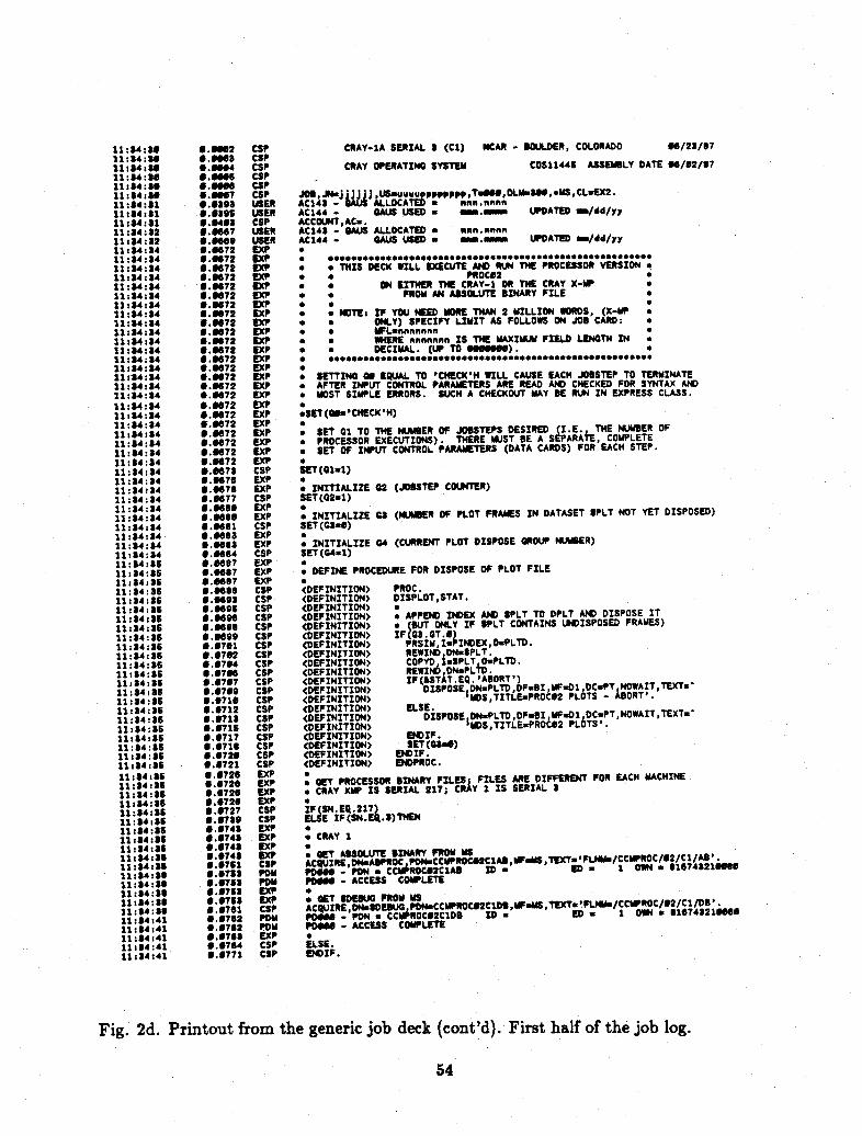
11:34:S3e · .e2 CSP CRAY-1A SERIAL 3 (Cl) NCAR - BOULDER, COLORADO 16/23/8711: 4:31 · .013 CSP11:34:83 6. i64 CSP CRAY OPERATING SYSTEM COS11445 ASSEMBLY DATE 6/012/8711 :34:4 0.e5s CSP11: 34:30 U .6 CSP11 * X4 ** * --- CSP11: 4:1 N .tl. 7 CSP JOB,JN.j J J US uuuupppppppp,TlM,.OLM.0,oMS,CLBEX2.11:34: 1 *.1393 USER AC143 - GAUS ALLOCATED a* nnnnnn11:34 :1 .O395S USER AC144 - AU USED . UPDATED m/dd/yy11:34:11 0.043 CSP ACCOUNT,AC-.11:14:12 .67 USER AC14 - GAUS ALLOCATED a nn.in11:14:32 0.669 USER AC144 - GAUS USED m. mm UPDATED _m/dd/yy11:14:34 ."672 EXP .11: 84: 34 · .0672 EXP .* *..e eeoeeo.*e.O.*Oe.SSo**o ****OS*S o o o o

11:34:34 *.672 EXP I THIS DECK WILL EXECUTE AND RUN THE PROCESSOR VERSION *

11: 4:34 J. 72 EXP * PROCI211:84:i 4 1.672 EXP · ON EITHER THE CRAY-1 R THE CRA Y X-MP11:4:34 .1672 EP * FROM AN ABSOLUTE BINARY FILE11:4:U:4 . 72 EXP *11:84:a4 .672 EXP * · NOTE: F YOU NEED MORE THAN 2 MILLION WORDS, (X-MP11:34:34 ."672 EXP * * ONLY) SPECIFY LIMIT AS FOLLOWS ON JOB CARD:11:14*: 4 *.*672 EXP · * MFLunnnnnnn11: 4:14 *.072 EXP * * WHERE nnnnnnn IS THE MAXIMUM FIELD LENGTH IN *11:34:34 ;.672 EXP * * DECIMAL. (UP TO G*O6M1 ).11:34:34 .1672 EXP · **e***·*************e * **O**·************************11:34:84 ·. ?672 EXP *11:3l4:34 S."2 EXP * SETTING EQUAL TO 'CHECK'H WILL CAUSE EACH JOBSTEP TO TERMINATE

11:14:34 1 . 72 EXP * AFTER INPUT CONTROL PARAMETERS ARE READ AND CHECKED FOR SYNTAX AND

11:14:4 *.1-72 EXP · MOST SIMPLE ERRORS. SUCH A CHECKOUT MAY BE RUN IN EXPRESS CLASS.

11:34:84 1.1672 EXP .11:14:34 8.672 EXP *SET(Ol'CHECK'H)11: 34:34 0.6t72 EXP *11:34:34 1.172 EXP * SET 01 TO THE NUMBER OF JOBSTEPS DESIRED (I.E THE NUMBER OF

11:3l;4:4 .6t72 EXP * PROCESSOR EXECUTIONS). THERE MUST BE A SEPARAfE, COMPLETE

11:34:34 · .1f72 EXP * SET OF INPUT CONTROL PARAMETERS (DATA CARDS) FOR EACH STEP.

11:34:34 1."72 EXP11:34 :4 :.ST731 CSP SET(G1.1)11:34:34 1.1676 EXP *11:34:34 G.S76 EXP * INITIALIZE 02 (JOSTEP COUNTER)11:34: 34 *.1677 CSP SET(G221)11:34: 4 ."611· EXP ·11:34:S34 S.Sf EXP * INITIALIZE 3G (NUMBER OF PLOT FRAMES IN DATASET PLT NOT YET DISPOSED)

11:41:4 :.14 .81 CSP SET(G3a·)11:34:34 0.·163 EXP ·11:3434 0.H163 EXXP INITIALIZE 04 (CURRENT PLOT DISPOSE OROUP NUMBER)11:34:14 · .·6"84 CSP SET(G4.1)11:34 :365 .187 EXP *11 :4 :6 I.SS66 EXP M DEFINE PROCEDURE FOR DISPOSE OF PLOT FILE112:34:35 .t687 EXP11:4.34:35 0.18 CSP <DEFINITION> PROC.11:34: *. 0.S93 CSP (DEFINITION> DISPLOT,STAT.11:3 4:35 . 95S CSP (DEFINITION> -

11:34:3l5 .·696 CSP (DEFINITION> · APPEND INDEX AND IPLT TO DPLT AND DISPOSE IT

11:34:35 6. fS CSP (DEFINITION> (BUT ONLY IF SPLT CONTAINS UNDISPOSED FRAMES)

11:84 0 ~." · 99 CSP (DEFINITION>) F(3. aOT. L)11: 4:365 .0701 CSP (DEFINITION> PRSIM, INDEX,O.PLTD.11:3 4:3 6 8.1702 CSP <DEFINITION) REWIND DNwSPLT.11:3 4:3 6 0 .1704 CSP (DEFINITION> COPYD, i.PLT OuPLTD.11:34:3 6 6.7"6 CSP <DEFINITION> REWIND DN=PLTD.

11:4:35 1.1707 CSP <DEFINITION> IF(&STAT.EQ. 'ABORT')

11:4:36 6.T709 CSP (DEFINITION> DISPOSE DNPLTD,DFB, UMFi 1 DCPT, NOWAT,TEXT-

11:34:35 0.6716 CSP <DEFINITION> IMDS,TITLE·PROC2 PL6TS - ABORT'.

11:34:356 6.712 CSP (DEFINITION> ELSE.11:34:36 1.1713 CSP (DEFINITION> DISPOSE DNSPLTD,DFUB, MFD)1 DCaPT,NOWAIT,TEXT"^11:14:386 *.715 CSP <DEFINITION>) MDS,TITLEsPROCI2 PL6TS'.

11:14: 16 .717 CSP (DEFINITION) ENDIF.11:34: 15 .0718 CSP <DEFINITION> SET("=l)11:34: 8 5 .0720 CSP (DEFINITION> ENDIF.11:34:3 5 0.6721 CSP (DEFINITION) ENDPROC.

x11:34':35 6.?726 EXP c11:34:,35 .1726 EXP * GET PROCESSOR BINARY FILES FILES ARE DIFFERENT FOR EACH MACHINE

11:314:35 .s726 EXP * CRAY XMP IS SERIAL 217; CRAY I IS SERIAL 311:3,4:35 6.6726 EXP11:34:35 0.6727 CSP IF(SN.EQ.217)11:34:56 0.?739 CSP ELSE IF(SN.EQ.3)THEN11: 34:35 .T743 EXP *11:34:3l5 6.0743 EXP · CRAY 111:34:5 0. 743 EXP W

11:4:35 0.0743 EXP · GET ABSOLUTE BINARY FROM MS

11:,14:3II 5 1 71 C ACQUIRE,DNSABPROC PDntCCMPRO2C1A,F IMSA ,TEXTIFL

w' M/CCMPROC/

2/Cl/AB'

11:34:36 .t753 PDM PD0)0 - PON * CClROC62C1AB ID * ED * 1 OWN * 11674321·6 e6

11: 4;:1 .0751 PDM PD - ACCESS COMPLETE11:14:311 .0?75S EXP *11:34:36 6.0753 EXP * GET IDEDMG FROM MS

11: 34:361 0.6761 CSP ACQUIRE,DoNsIDEB PtONCCMPROC2C1B, IlMMS ,TEXT' FLNM'/CCMPROC/2/Cl/PBe'.

11:34:41 ·. ?762 PDM P0O66 - PODN CCPROCI2C1DB rD a ED a I D1N a 61674321166

11:34:41 0.6762 POM P066 - ACCESS COMPLETE11:34:41 0.67631 EXP11:84:41 6.764 CSP ELSE.11:34:41 0.?771 CSP ENDIF.

Fig. 2d. Printout from the generic job deck (cont'd). First half of the job log.

54

EXECUTE THE PROCESSO TERATIVELY FOR MULTIPLE JOBSTEPS

LOOP.EXITLOOP (2.GT. 1)ASPROC.

Z0048 - COPY OF 29 RECORDS i FILES COMPLETEDP006 - PON a MCCM1223X22301 ID a CSM ED * 0OWN a 732209023402P0669 - DATASET NOT FOUNDMS00H - 64664664 BYTES READ TO CSM/MCCM1223X22301P00D0 - PDN a MCCM1223X22301 ID a CSM ED a 1 OW · l168743210080tPO6 - ACCESS COMPLETE

1O046 - COPY OF 1I RECORDS 1 FILES COMPLETED1004 - COPY OF 176 RECORDS I FILES COMPLETED1048 - COPY OF 168 RECORDS I FILES COMPLETEDUT010 - STOP IN CRAYPR

SET (02G02*1)ENDLOOP.

EXITLOOP (02.T.01)

CALL PROCEDURE TO DISPOSE ANY PLOTS NOT YET DISPOSEDDISPLOT,'NORM'.

* APPEND INDEX AND SPLT TO DPLT AND DISPOSE IT(BUT ONLY IF IPLT CONTAINS UNDISPOSED FRAMES)

IF(G3 .T.8)ENDIF.

EXIT.END OF JOB

JOB NAME - SAP4241USER NUMBER - uuuupppppppTIME EXECUTING IN CPU - 6666:6:04.8683TIME WAITING TO EXECUTE - 606N:63:24.6216TIME WAITING FOR I/O - 0660:00:06.6244TIME WAITING IN INPUT QUEUE - 6":60:006.01666MEMORY * CPU TIME (MWDS*SEC) - 1.78273MEMORY * I/O WAIT TIME (MWDS.SEC) - 0.94061MINIMUM JOB SIZE (WORDS) - 36MAXIMUM JOB SIZE (WORDS) - 401408MINIMUM FL (WORDS) - 36362MAXIMUM FL (WORDS) - 97312MINIMUM JTA (WORDS) - 3684MAXIMUM JTA (WORDS) - 496MAXIMUM OPEN DISK SECTORS - 21463DISK SECTORS MOVED - 1746USER I/O REQUESTS - 134OPEN CALLS - 19CLOSE CALLS - 14MEMORY RESIDENT DATASETS - 0TEMPORARY DATASET SECTORS USED - 1PERMANENT DATASET SECTORS ACCESSED - 21423PERMANENT DATASET SECTORS SAVED - 0SECTORS RECEIVED FROM FRONT END - 6SECTORS QUEUED TO FRONT END - 64

CPU HOURS -lOW HOURS -AVG MEMORY (MWD) -DD19 ACTIVITY (I/O REQ) -

* (MDS .MOVED) -

8.061366.661400.27666

134.689344

GAU COMPONENTSJOB CHARGE -CPU CHARGE -tOW CHARGE -MEMORY CHARGE -

DISK ACT CHO -

TOTAL CHARGE BEFORE CLASS FACTOR (EXCL.NS/TAPE/NTWK) -MULTIPLIER FOR CLASS EX2 - 2.66MULTIPLIER FOR Cl ALLOCATION - 0.68

6AUS CHARGED AGAINST ALLOCATION -

06.61908 ."1660 .004660.0611

.66.040

.00441

Fig. 2e. Printout from the generic job deck (cont'd). Second half of the job log.

55

11:84:4111:34:4111:34:4111:34:4111:34:4111:34:4711:35:0611:36:6811:36:0611:37:6511:37:6711:37:5711:38:0211:36:0211:38:0311:38:0311 :3 :0311:38:0311:38:0311:38:6311:38:0311:38:0311:38:0311:38:0311: 38:311:38:0311:38:0311:36:0311:38:0311:38:0311:38:0311:38:0311:36:0311:38:0311:38:0311:38:0311: 3:0311:38:0311:3 :0311:38:0311:38:0311:38:0311:38:0311:38:0311:38:0311:38:0311:38:0311:386:0311:368:0311:368:6311:38:0311:38:0311:38:0311:38:0311:38:0311:38:0311:36:0311:38:0411:38:0411:38:0411:38:0411:38:0411:38:0411:38:0411:38:0411:38 :0411:38:6411:38:0411:38:6411:38:04

06.77 EXP.6773 EXP.6773 EXP.8774 CSP

6.6777 CSP.68769 CSP

1.4396 USER1.5996 POM1.6998 PDM1.5996 TBT1.5996 POM1.599" POM4.8 13 USER4.8211 USER4.8320 USER4.8461 USER4.8462 CSP4.8456 CSP4.6462 CSP4.1470 EXP4.6470 EXP4.4866 CSP4.5664 1 EXP4.5664 1 EXP4.8664 1 EXP4.S666 1 CSP4.8568 1 CSP4. 6571 EXP4.8672 CSP4. 573 CSP4.8674 CSP4.IS76 CSP4.6566 USER4. 666 USER4.8687 USER4. 66S USER4.8688 USER4.8669 USER4. 690 USER4. 691 USER4. 692 USER4.6593 USER4. 694 USER4. 694 USER4.8696 USER4.8S96 USER4.8697 USER4.6597 USER4.6698 USER4. 699 USER.4.668 USER4.688" USER4.6661 USER4.6662 USER4.6603 USER4. 6803 USER4. 604 USER4.6669 USER4.6069 USER4.6610 USER4.6612 USER4.0613 USER4. 614 USER4.6615 USER4.8616 USER4.6617 USER

4.8616 USER4.6619 USER4. "20 USER4.0621 USER

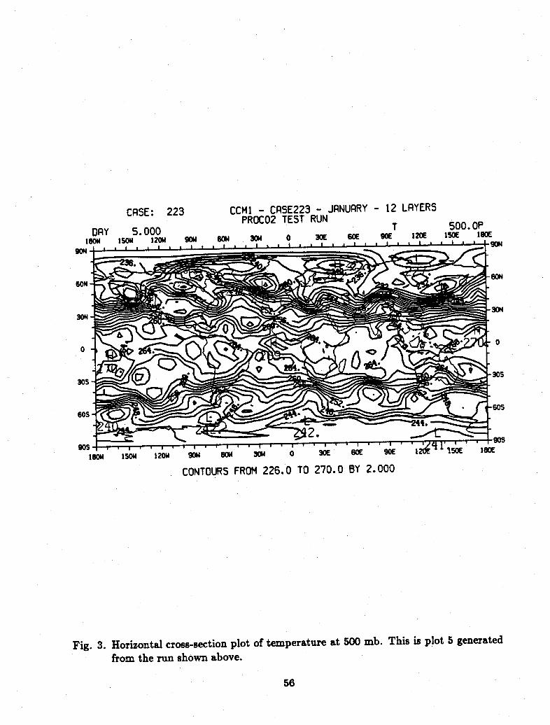
CASE: 223 CCM1 - CASE223 - JANUARY - 12 LAYERSPROCO2 TEST RUN

DAYv 5.000 T 500. O104 IS4 120 904m 604 304 0 30E 6SC 9oE 120C IS 1 I8C

- . . . .. A , . .a a a aa t a a a I I a a - a I a Lq gm

O1 0 1 351 N l W wg . .

CONTOURS FROM 226.0 TO 270.0 BY 2.000

Fig. 3. Horizontal cross-section plot of temperature at 500 mb. This is plot 5 generated

from the run shown above.

56

I 0. P

200. OP

400.OP

500.OP

600. OP

700.Op

900. OP40.0

CRSE: 223 CCM1 - CRSE223 - JANUARY - 12 LRYERSPROC02 TEST RUN

DRY 5.000 TZONRL RVERAGE FROM -180.0 TO 172.5 DEGREES

CONTOURS FROM 186.0 TO 288.0 BY 6.000

Fig. 4. Latitudinal cross-section plot of the zonally-averaged temperature field. This is

plot 10 generated from the run shown.

57

5.0 Summary

The modular processor is an extensive post-processing tool for CCM and CCM historytape format output data. The processor can be controlled by a series of input controlparameters (ICPs), and decks of ICPs can be constructed to generate printed and plottedoutput and/or other datasets. The information given here serves as an introduction to theuse of this post processor.

Hopefully, this tutorial has answered basic questions related to the use of the CCM modularprocessor. Any questions related to the processor can be directed to:

Mike Dias ........................... (303) 497-1349Rick Wolski .......................... (303) 497-1330Gloria Williamson . ...................... (303) 497-1380

We will gladly answer your questions or problems. Also, please report any discoveredproblems in the processor to Rick Wolski or Mike Dias, or send a MAIL message to WOLSKIon the IBM 4381. By periodically browsing the CCM NEWS file on the CSMLIB machine,you will be informed of any important processor updates. Please feel free to request writtencopies of any processor updates.

58

REFERENCES

Bath, L.M., M.A. Dias, D.L. Williamson, G.S. Williamson and R.J. Wolski, 1987: Users'Guide to NCAR CCM1, NCAR Technical Report, NCAR/TN-286+IA.

Williamson, D. L., J.T. Kiehl, V. Ramanathan, R.E. Dickinson and J.J. Hack, 1987:Description of NCAR Community Climate Model (CCM1), NCAR Technical Report,NCAR/TN-285+STR, 112 pp.

Wolski, R., 1987: CCM Modular Processor Users' Guide (Version PROC02). NCARTechnical Report, NCAR/TN-290+IA.

59

Documents

NCAR/TN-289+IA Introduction to the CCM Modular Processor