NBER WORKING PAPER SERIES

RISING IMPORT TARIFFS, FALLING EXPORT GROWTH:WHEN MODERN SUPPLY CHAINS MEET OLD-STYLE PROTECTIONISM

Kyle HandleyFariha KamalRyan Monarch

Working Paper 26611http://www.nber.org/papers/w26611

NATIONAL BUREAU OF ECONOMIC RESEARCH1050 Massachusetts Avenue

Cambridge, MA 02138January 2020, Revised August 2020

The Census Bureau's Disclosure Review Board and Disclosure Avoidance Officers have reviewed this data product for unauthorized disclosure of confidential information and have approved the disclosure avoidance practices applied to this release (DRB Approval Numbers: CBDRB- FY19-519, CBDRB-FY20-104, CBDRB-FY20-CES006-004, CBDRB-FY20-CES006-005). We thank Chad Bown, Teresa Fort, Colin Hottman, Soumaya Keynes, CJ Krizan, Frank Li, and seminar and conference participants at the Federal Reserve Board, University of Michigan, Mid-Atlantic International Trade Workshop, U.S. Census Bureau, Stanford University, University of Virginia, Georgetown University, George Washington University, IDB, Rowan University, and FREIT ETOS for helpful comments and discussions. Any opinions and conclusions expressed herein are those of the authors and do not necessarily represent the views of the U.S. Census Bureau, other members of the research staff at the Board of Governors, the Board of Governors of the Federal Reserve System, or the National Bureau of Economic Research.

NBER working papers are circulated for discussion and comment purposes. They have not been peer-reviewed or been subject to the review by the NBER Board of Directors that accompanies official NBER publications.

© 2020 by Kyle Handley, Fariha Kamal, and Ryan Monarch. All rights reserved. Short sections of text, not to exceed two paragraphs, may be quoted without explicit permission provided that full credit, including © notice, is given to the source.

Rising Import Tariffs, Falling Export Growth: When Modern Supply Chains Meet Old-Style ProtectionismKyle Handley, Fariha Kamal, and Ryan MonarchNBER Working Paper No. 26611January 2020, Revised August 2020JEL No. F1,F13,F14,F23,H2

ABSTRACT

We examine the impacts of the 2018-2019 U.S. import tariff increases on U.S. export growth throughthe lens of supply chain linkages. Using 2016 confidential firm-trade linked data, we identify firmsthat eventually faced tariff increases. They accounted for 84% of all exports and represented 65%of manufacturing employment. For the average affected firm, the implied cost is $900 per worker innew duties. We construct product-level measures of exporters' exposure to import tariff increases andestimate the impact on U.S. export growth. The most exposed products had relatively lower exportgrowth in 2018-2019, with larger effects in 2019. The decline in export growth in 2019Q3, for example,is equivalent to an ad valorem tariff on U.S. exports of 2% for the typical product and up to 4% forproducts with higher than average exposure.

Kyle HandleyRoss School of BusinessUniversity of Michigan701 Tappan StreetAnn Arbor, MI 48109and NBERhandleyk@umich.edu

Fariha KamalU.S. Bureau of the Census4600 Silver Hill RoadWashington, D.C 20233fariha.kamal@census.gov

Ryan MonarchInternational Finance DivisionFederal Reserve Board of Governors20th Street and Constitution Avenue N.W.Washington, D.C. 20551ryan.p.monarch@frb.gov

1 Introduction

The United States imposed a series of wide-ranging increases in import tariffs from 2018

through 2019. By August of 2019, $290 billion of U.S. imports - about 12% of the total

- were subject to an average tariff increase of 24 percentage points.1 The scale of these

tariffs against specific products and countries, and the subsequent retaliation, has drawn

comparisons to the Depression-era tariff wars of the 1930s.2 However, the structure of

world trade has been substantially transformed since then, following reductions in trade

costs and new communications technology (Baldwin, 2016). Global supply chains are a

pervasive feature of world trade (Hummels, Ishii and Yi, 2001; Johnson and Noguera, 2017)

and a potentially important channel of transmitting the impact of import tariffs to exports

because they can amplify shocks to trade costs and demand across locations (Almunia,

Antras, Lopez-Rodriguez and Morales, 2018; Boehm, Flaaen and Pandalai-Nayar, 2019; Yi,

2003). We estimate and quantify the supply chain spillovers to export growth of increases

in U.S. import tariffs.

Notably, U.S. export growth was weak from mid-2018 through late 2019. Figure 1

illustrates the average 12-month export growth rate for each quarter from 2017 and shows

that export growth declined beginning in 2018 Q4.3 The drop in export growth extends

beyond the major products and countries that were the focus of 2018-2019 trade tensions:

the decline is clear even when progressively excluding products that ultimately face foreign

retaliation; all remaining exports to China, Mexico, and Canada; and finally all remaining

trade with Asia and Europe. The wide-ranging weakness in U.S. export growth underlines

the importance of quantifying the supply chain spillovers of import tariffs.

We demonstrate that U.S. import tariffs weakened U.S. export growth leveraging confi-

dential U.S. firm-trade linked data. First, we measure the firm-specific incidence of the tariffs.

Then, we identify the set of exporters that are also importing products in the same cate-

gory on which tariffs are ultimately imposed in 2018-2019 to construct measures of import

tariff exposure for dis-aggregated export products. Finally, combined with official monthly

public-use export data from 2015 through 2019, we estimate the impacts of exposure to

increases in import tariffs. We find that supply chain spillovers from increased import tariffs

1The dollar value of tariffed imports is calculated on an annual basis using 2017 data, and the averagetariff increase is weighted using the same data. For a timeline of tariffs on U.S. imports and foreign retaliatoryexport tariffs, see Bown and Kolb (2019).

2The Smoot-Hawley tariffs increased import duties by about 20% on average and set off a wave ofworldwide protectionism (Irwin, 1998).

3For every month of U.S. export data and every destination country–HS 6-digit product pair, we computethe 12-month growth rate, then take the average within each quarter.

dampened U.S. export growth over 2018-2019 for the typical affected export product, even

after controlling for foreign-imposed retaliatory export tariffs.

Our findings are consistent with U.S. export growth weakening in response to newly

imposed import tariffs that impacted firms’ supply chain networks. U.S. tariff increases

were disproportionately applied to intermediate goods that are typically inputs in production

(Bown and Zhang, 2019). Lovely and Liang (2018) document that the Section 301 import

tariffs taxed inputs for U.S. businesses via supply chain trade. Amiti, Redding and Weinstein

(2019) estimate that $165 billion in trade may have been lost when firms redirected trade in

their supply chains to avoid tariffs. Our results are also consistent with business anecdotes.

For example, in U.S. Senate testimony, the CEO of Learning Resources wrote: “We have

business reasons for the assignment of products to specific factories, whether in the United

States or in other countries. [...] We have also made repeated attempts to develop a U.S.-

based supply chain but cannot do so on any basis, even inefficiently. We have no known

realistic alternative to our current supply chain.”(U.S. Senate Committee on Finance, 2018).

Caldara, Iacoviello, Molligo, Prestipino and Raffo (2019) find that when firms discussed

tariffs and policy uncertainty on earnings calls in recent years, the primary concern cited

was their supply chains. The Federal Reserve Beige Book (November 27, 2019) documents

that “[...] firms have reported tariff impacts on sales, either in terms of pricing or in terms

of supply chain disruptions slowing their product supply.”

The first part of the paper documents tariff incidence within and across firms by linking

the publicly available information on new tariffs to data on the operations of firms importing

or exporting, in 2016, those products that would ultimately face tariff increases.4 About a

third of all U.S. importers in 2016 traded product categories that would be exposed to the new

import tariffs in 2018-2019 and they employed 32% of all non-farm, private sector workers.

About 19% of U.S. exporters faced retaliatory foreign export tariffs and they employed 23%

of all non-farm, private sector workers. A non-trivial share of trade value was subject to

tariff increases at the typical affected firm: 46% of an affected importer’s purchases were

subject to U.S. import tariffs; and 33% of an affected exporter’s sales faced foreign export

tariffs.

Next, we document important sources of heterogeneity across firms hit by new import

and export tariff increases. We find that U.S. importers facing import tariff increases em-

ployed twice as many workers compared to the average importing firm and about nine times

as many workers as the average firm. Similarly, we find that U.S. exporting firms facing

4Our exposure measures leverage trade patterns well before the 2016 presidential election outcome wasknown and prior to the anticipation of new tariffs throughout 2017.

2

retaliatory tariffs were more than three times larger than the average exporting firm. Thus,

the tariff increases hit the very largest trading firms in the U.S. economy.

The tariff costs are non-trivial for the average firm in the economy: assuming that tariffs

remained in place for a full year and firms did not adjust sourcing strategies, the implied

duties paid were $900 per worker overall and about $1,600 per worker in the manufacturing

sector. Workers in manufacturing and retail were most exposed to the import tariff increases:

65% of employment in manufacturing and 60% of employment in retail was at firms facing

higher import tariffs.

The vast majority of U.S. trade is conducted by firms that both export and import.5 We

find that, based on 2016 trade flows, U.S. exporters exposed to import tariffs in the same

broad product category as their exports - products mostly likely to be part of a supply chain

- accounted for 43% of total U.S. exports and 24% of all U.S. exporters. Considering U.S.

exporters exposed to any import tariff, the share of affected export value nearly doubles to

84%.

We aggregate individual U.S. exporters’ exposure to increases in import tariffs to con-

struct product level measures of import tariff exposure. We then estimate the impact of

import tariff exposure on U.S. export growth in a generalized difference-in-differences frame-

work. Using publicly available trade data from 2015 through 2019, we regress the 12-month

change in exports at the product-country level on product-specific variation in import tariff

exposure measures while controlling for potential foreign retaliatory tariffs that those ex-

ports may have faced. We estimate a differential in growth rates in high relative to low

exposure products (first difference) in the period before and after the waves of new import

tariffs (second difference).6

We find that average bilateral export growth at the country-product level was lower

in products with a higher share of exporters subject to import tariff increases. We further

trace out the timing of these effects by interacting the import tariff exposure measure with

quarterly indicators. We find that exposure depresses export growth in 2018 and especially

2019. Exported products with average exposure had a growth rate of about 0.75 log points

lower than an unaffected products in 2018 and about 1.3 log points lower in 2019. By 2019,

this magnitude is equivalent to an ad valorem tariff on U.S. exports of almost 1.5% for the

average country-product export. For sectors with exposure two standard deviations above

5The top 1 percent of U.S. traders account for more than 80 percent of total U.S. trade (Bernard, Jensen,Redding and Schott, 2018).

6We measure exposure at the HS 6-digit product level, which is the most dis-aggregated product codethat is consistent across countries and time. The retaliatory export tariff data is linked to U.S. export flowsat the the HS 6-digit product level.

3

the mean, depending on which yearly effects are used, this implied ad valorem equivalent

tariff is 3-4%, close to the average, statutory MFN tariff rates imposed on trade partners by

the U.S. and E.U.

This paper makes three main contributions. First, to our knowledge we are the only

paper to use linked U.S. firm-trade transactions data to assess the incidence of the 2018-

2019 tariffs on firms, jobs, sectors, and export growth using aggregated measures of firms’

supply chain networks. We thus broaden our understanding of the impacts of the 2018-2019

tit-for-tat tariff wars in an era of outsourcing and global production fragmentation. Our

contribution is complementary to several recent papers that study the incidence of the 2018-

2019 tariffs.7 Flaaen, Hortacsu and Tintlenot (2020) estimate that tariff increases caused

washing machine prices to rise by 12 percent. Amiti, Redding and Weinstein (2019) and

Fajgelbaum, Goldberg, Kennedy and Khandelwal (2020) study the direct impacts of the

2018-2019 U.S. import tariff increases on U.S. import prices and the direct impact of the

foreign retaliatory tariff increases on U.S. export prices. Cavallo, Gopinath, Neiman and

Tang (2019) also examine the passthrough of U.S. import tariff increases to U.S. importers

and retailers using firm-level data. However, these studies do not consider spillover effects

of increases in U.S. import tariffs on U.S. exports through supply chains.8 Our estimates

suggest accounting for supply chain linkages would likely increase the welfare costs of the

2018-2019 U.S. tariff increases.

Second, our results demonstrate that firms’ reliance on global supply chains can com-

plicate the application of traditional mercantilism – trade policy that aims to improve the

balance of trade by reducing imports and promoting exports. In a counterfactual exercise,

we find the reduction in export growth would have been attenuated by 35% if the tariffed

products were not part of tightly linked supply chains. Blanchard, Bown and Johnson (2016)

show that global supply chains, which increase the foreign content embodied in domestic fi-

nal goods, should lower a government’s incentive to impose tariffs on inputs. Our results

provide empirical motivation for that incentive, but highlight how designing the optimal tar-

7Several papers have examined non-trade outcomes. Waugh (2019) studies the impact of Chinese retal-iatory tariffs in 2018 on U.S. consumption to find that counties more exposed to Chinese tariffs experienced2.5 percentage points lower growth in auto sales compared to counties with lower exposure. Blanchard,Bown and Chor (2019) study the impact of a county’s exposure to U.S.-imposed import tariffs and foreignretaliatory export tariffs on the county’s Republican vote share in the 2018 U.S. House elections. Flaaenand Pierce (2019), using aggregated input-output tables, examine the effect of higher input costs from the2018-2019 U.S. import tariffs on domestic output and employment in the U.S. manufacturing sector; whileBown, Conconi, Erbahar and Trimarchi (2020) carry out a similar analysis but consider the supply chaineffects of anti-dumping duties.

8An exception is Benguria and Saffie (2019) who study the impact of tariffs and uncertainty on U.S.exports. However, the authors use aggregated input-output tables to measure input tariffs.

4

iff policy may be difficult in practice. For example, the first phase of import tariff increases

on Chinese products under Section 301 were intended to target specific Chinese products

where U.S. consumers and businesses had alternative country sourcing options (U.S. Senate

Committee on Finance, 2018). But our findings suggest that firms were unable, at least

in the short-term, to reorient sourcing strategies, perhaps because buyer-seller relationships

embody relationship specific investments and capital cannot easily be replaced by alternative

foreign and domestic sourcing.9

Finally, we make a novel methodological contribution. Confidential firm-transaction

linked data is available with much longer processing lags (typically two years or more in

the U.S.) that prohibits contemporaneous analyses of firm-level impacts of the 2018-2019

tariffs. But the trading status of large firms is persistent. Moreover, even if individual firms

enter and exit international markets, population moments constructed from the cross-section

of firm-level data should be representative of the firm trade participation at an industry

level, which provides a sufficient basis for constructing our import tariff exposure measure

capturing supply chain linkages. We show that nearly contemporaneous, public-use monthly

trade data can be combined with data moments derived from the rich, underlying detail in

firm-level micro data to evaluate policy changes. Our approach could be extended to better

inform the policy making process in international trade and other economic applications.

The rest of the paper is organized as follows. Section 2 describes our data sources

and provides summary statistics on U.S. importers facing import tariffs and U.S. exporters

facing retaliatory foreign export tariffs. We describe the empirical approach in Section 3 and

present the results in Section 4. Section 5 concludes.

2 Measuring the Impact of Tariffs with Firm Data

We link confidential micro data on U.S. trading firms to publicly available lists of product

codes subject to newly imposed import and export tariffs. Thus, we can determine which

firms are being directly affected by import and export tariffs. We combine information on

the value, quantity, and HS product code traded by firms as well with their employment,

number of establishments, age, and sector of operation.

9The cost of switching suppliers may be very high as demonstrated by Monarch (2016) in the context ofbuyer-supplier relationships in U.S.-China trade.

5

2.1 Timing and Characteristics of New Tariffs

We construct a database of monthly U.S. import tariffs at the HS 8-digit level from publicly

available tariff schedules published by the U.S. International Trade Commission. For all

tariff increases since the beginning of 2018 through 2019, we keep track of the HS code, the

new tariff rate, and the date of the change.10

Multiple lists of tariff lines were circulated weeks or more in advance of implementation.

In the case of China, the lists were often modified on the date of implementation and products

added or dropped in subsequent Federal Register notices. The lists of new import tariffs are

so broad that some tariffed products are not even imported by the U.S. from China or any

other country. However, for every newly tariffed country-product pair that is traded, there

must be at least one firm facing a potential supply chain disruption or some form of higher

costs, e.g. actual duties paid, a new sourcing decision, or even lobbying for exemptions.

The scope and timing of the import tariffs is show in Figure 2. We match the new tariff

lines, at the HS 8-digit level, by date in 2018-2019 to country-product level annual import

totals in 2016.11 Over 10,000 country-product pairs, more than half coming from China,

are ultimately affected. Firms may import multiple affected products and products may be

imported across multiple sectors such as manufacturing, services, or retail. Moreover, many

of the tariff waves and escalations were threatened, then modified or delayed (sometimes

indefinitely) before the precise implementation date shown on the graph. The uncertainty

about timing of implementation, the duration of the tariffs, and which products would be

on the final lists may have been an additional source of disruption to firms.

An important feature of the tariff increases was that they fell mainly on intermediate

goods. For all affected products, the tariff increased by an average of about 24 percentage

points over 2018-2019. Intermediate goods represent 56.8% of the total value of goods

receiving tariffs, compared to 27.3% for capital and 15.6% for consumption goods.12 This

is especially salient in the case of tariffs against Chinese imports. Under the Section 301

tariffs, 82% of all intermediate goods imported from China had received tariffs by May 2019

(Bown, 2019). In comparison, the share of new tariffs on capital and final goods sourced

from China were only 38% and 29%, respectively.

U.S. tariff increases on different countries and products were often followed by retaliation

against U.S. exporters. For this reason, we also construct a database of retaliatory foreign

10Fajgelbaum, Goldberg, Kennedy and Khandelwal (2020) have a summary of the timeline of the wavesof tariff increases and affected products. See Appendix A for more details on the tariff lists in our data.

11We use 2016 as a base year to match our firm-trade transactions data linkage below.12These are value value-weighted tariff increases and trade shares using 2017 annual import data. We use

the United Nation’s Broad Economic Classification to classify goods.

6

export tariffs at the 6-digit HS (HS6) level using the timeline from Bown and Zhang (2019).

The trade-weighted average tariff increase from retaliation is about 20 percentage points and

affects around 8% of total U.S. exports.13 The average change in exports for all countries

and products is effectively zero. But for affected export products, the average annual change

over 2018-2019 is about 13 log points in our regression sample (see Appendix Table A-2).

Nevertheless, as show in Figure 1, foreign retaliation alone does not explain a slowdown in

U.S. export growth during this period.

We summarize these features at the firm-level in the next section before turning to our

estimation strategy.

2.2 Firm-Level Trade and Employment Data

We draw U.S. firm-level trade and employment characteristics from two sources of confiden-

tial microdata covering the universe of merchandise trade transactions and non-farm, private

sector employers.

The Longitudinal Firm Trade Transactions Database (LFTTD) contains transaction-

level detail on the universe of imported shipments valued over US$2,000 and exported ship-

ments valued over US$2,500 of merchandise goods. Using the 2016 LFTTD, we identify U.S.

exporters and importers and link the firms directly to the U.S. import tariff and foreign

retaliatory export tariffs imposed in 2018-2019 at the country-HS6 product-month level.

We construct the import tariff exposure measure using 2016 trade data for two reasons.

First, it minimizes concerns that our measure may be contaminated by any anticipatory or

policy uncertainty induced factors influencing firms’ decisions in advance of tariffs actually

being imposed. Using 2016 predates the outcomes of the U.S. presidential election for most

of that year or any anticipatory affects in 2017. Second, contemporaneous exposure measures

may reflect endogenous firm-level responses to the trade policy changes. These include exit

from sourcing in some foreign markets and entry into others induced by the policy change.

We use the 2016 LFTTD to describe the firm-level incidence of the 2018-2019 tariff

increases because importing and exporting are very persistent activities. Firms we identify

as being affected by the tariffs using 2016 data are very likely to be affected in the years tariffs

are actually imposed. The implication is that the cross-section, population level statistics of

2016 firm characteristics should be representative at the aggregate and industry-aggregate

level of import and export exposure to future tariffs, even if firms responded to the policy

13Figures calculated using 2017 trade weights and exclude retaliation after the September 1, 2019 U.S.tariff increases. Additional details in Appendix A.

7

change in 2018, for instance, by terminating imports from a source country. As a robustness

check, we also augment our exposure measures with data from the 2014 and 2015 LFTTD.

We match trading firms in the LFTTD to the Longitudinal Business Database (LBD).

The LBD tracks all U.S. establishments in the non-farm, private sector employer universe

over time (Jarmin and Miranda, 2002).14 It contains information on every establishment’s

firm affiliation, year of birth (used to construct firm age), industrial activity at the six-digit

NAICS level, employment, and payroll.

2.3 Characteristics of Affected Importers and Exporters

Table 1 presents a broad picture of how U.S. importers and exporters, as identified in 2016,

were affected by the 2018-2019 tariffs. Taking all of the newly imposed U.S. tariffs in 2018

through 2019, affected imports represented 11.2% of total imports (about $247 billion) and

almost a third of all importing firms. The affected firms employed 32% of all U.S. non-

farm private sector workers. For the average affected importer, 46.5% of their import value

was subject to import tariff increases. In the aggregate, all of the newly imposed foreign

retaliatory export tariffs in 2018 through 2019, affected 8% of U.S. exports in LFTTD (about

$115 billion) and 18.7% of all exporting firms. These exporting firms employed about 23% of

all non-farm private sector employees.15 For the average affected exporter, about one third

of their export value was subject to foreign retaliatory tariff increases.

Panel A in Table 2 presents characteristics of firms importing products in 2016 that

would face U.S. import tariff increases in the 2018-2019 period. The average importing firm

facing tariffs was about twice as large as the average importer, both in terms of employment

(430 vs. 212 workers) and the number of establishments (9 vs. 5). Comparing the last two

columns illustrates the well-known fact that importers exhibit a significant size premium

relative to the average firm and indicates that U.S. import tariffs overwhelmingly impacted

the largest firms in the U.S. economy. The age profile of affected importers is very similar

to all importers; and the typical annual pay for workers at firms facing import tariffs is also

comparable, about $58,000 per worker.

We carry out a similar breakdown for U.S. firms facing retaliatory tariffs from foreign

countries in Panel B of Table 2. Affected exporters were two to three times as large as the

average exporter, using employment or the number of establishments. Retaliatory tariffs fell

14LBD excludes operations with no statutory employees, e.g. self-employed, farms (but not agri-business),and the public sector. At the time of this study, the most recent available year of the LBD is 2016.

15Since many firms both import and export, this share is not mutually exclusive from the share of workersaffected by import tariffs.

8

on some of the largest firms in the U.S. economy. The impacted exporters exhibited higher

average earnings and were also older compared to the average exporter.

2.4 Characteristics of Affected Sectors

Linking the trade data to firm-level characteristics also enables an examination of the most

affected sectors. We identify which firms in 2016 are trading products that face tariff in-

creases in 2018-2019 and aggregate up to broad sectors using firm industry and employment

information.

We report summary statistics, in Table 3, on the share of workers impacted by the

increase in U.S. tariffs and average duties paid per worker overall and across four broad

sectors: manufacturing, wholesale, retail, and other.16 In some of the sectors most affected

by U.S. import tariffs, such as manufacturing and retail, upwards of 60% of workers are

employed at firms facing tariff increases. This is in contrast to sectors included in “Other”

where relatively few workers are employed at affected firms, including firms providing services

or agricultural operations.17 In the second column, we observe similar sectoral rankings in

the share of workers that were most exposed to increases in foreign retaliatory export tariffs.

The third column of Table 3 shows the implied average duty per worker by sector.

This measures the total tariff bill of all affected firms in a sector divided by the number of

workers in that sector.18 To the extent that these imputed tariffs can be interpreted as a

direct increase in costs, manufacturing firms potentially paid about $1,600 in tariffs for each

worker, while wholesale firms paid closer to $5,000 per worker.19 The typical affected firm

in the economy paid about $900 per worker in tariffs. Using payroll (earnings) per worker

from Table 2, the implied duties were equivalent to 1.5% of the average wage bill.

16Manufacturing is defined as all sectors within NAICS 31-33; Wholesale is defined as all sectors withinNAICS 42; Retail is defined as all sectors within NAICS 44 and 45; and Other includes all other sectorsexcept 92 (Public Administration).

17Some reports indicate that individual farmers may be negatively affected by new tariffs (see Bunge etal. (2019), for example), but the the LBD only covers non-farm sectors.

18Total tariffs paid are imputed based on total imported value of tariffed products in 2016 times therespective tariff increase as of April 2019. The calculation assumes that the import tariff burden is borneas an additional cost for U.S. firms. Conditional on maintaining import volumes at 2016 levels, the impliedvalues are consistent with evidence of complete passthrough of the tariffs to U.S. firms (Amiti, Redding andWeinstein, 2019; Fajgelbaum, Goldberg, Kennedy and Khandelwal, 2020; Cavallo, Gopinath, Neiman andTang, 2019).

19Although a large fraction of retail workers were employed at affected firms, the overall per-worker burdenon these firms was fairly small because tariffs fell mainly on imported intermediates rather than consumergoods.

9

2.5 Import Tariffs and U.S. Exporters

The broad coverage of intermediate goods subject to the 2018 and early 2019 import tariffs

means that firm-level supply chains were more likely to be directly affected relative to con-

sumer products. The official Federal Register notice of tariff increases in April 2018 indicates

that tariffed products were chosen by “selecting products [...] with lower consumer impact”

(Federal Register, April 6, 2018).

Linking import and export activity at the firm level reveals the extent to which supply

chains were potentially impacted. We consider three distinct definitions of exposure to import

tariff increases. We begin by defining exporters to be affected if they face new import tariffs

on any product, capturing an overall increase in input costs at the firm level. Under this

measure, 84% of total U.S. exports were by firms facing import tariff increase on at least one

product. The share of affected firms is smaller, 24%, but these exporters tend to be larger

than average. However, all exports of an affected firm may not be impacted by import tariff

increases, especially if the affected products are a small share of an exporter’s import basket.

Another approach is to consider whether a firm’s exported products are in the same

broad product category as its imported products facing new import tariffs. To operationalize

this, we define exporters to be affected only if they face new import tariffs in a HS6 product

within the same 4-digit HS (HS4) chapter as their exports. Using this approach, 43% of U.S.

exports are subject to the new import tariffs within related product groups, representing

13% of all U.S. exporters. Finally, we make the connection between the tariffed imports

and exports of the firm even tighter by defining exporters to be affected only if they face

new import tariffs in the same HS6 product as their exports. Under this definition, close to

one-third of U.S. exports and 10% of U.S. exporters are potentially affected by U.S. import

tariffs. Table A-1 includes a complete summary of these measures.

Imports of products in the same product groups as a firm’s exported products should

more closely measure supply chain linkages due to foreign sourcing or offshoring.20 The main

idea is that closer the inputs are to the final output product classification, the more likely it

is that the U.S. firm could have produced these inputs. Our approach relates directly to the

Hummels, Jørgensen, Munch and Xiang (2014) measure of firm-level offshoring as imports

of products in the same HS4 heading as the firm’s output. This is our “baseline” definition

to identify supply chain linkages. Bernard, Fort, Smeets and Warzynski (2020) measure

firm-level offshoring as imports of products in the same HS6 category as the firm’s output,

20Hummels, Munch and Xiang (2018) define three elements of offshoring: (i) intermediate inputs used forproduction; (ii) imported inputs; and (iii) inputs that could have been produced internally within the samefirm.

10

which we will call a “narrow” definition of supply-chain linkages, while we will refer to the

measure capturing all exports by firms facing any import tariffs as “broad”. We establish

the robustness of our results using all three definitions. We also provide empirical tests of

the strength of the supply-chain linkages implied by each definition.

3 Empirical Framework

We construct product-level, population statistics on exposure to increases in import tariffs

by U.S. exporters. We first describe the measures and then aggregate up from the firm-level

to various product-level exposure statistics. We then use these product-level measures to

estimate the impact on export growth at the country-product level.

3.1 Import Tariff Exposure

We begin by constructing product exposure measures from the cross-section of 2016 ex-

porters. We show that the measures share useful aggregation properties and are related

to differential trends in U.S. export growth across the most exposed and all other product

groups.

We construct measures of exposure by 6-digit HS product codes.21 First, we count the

number of unique exporters in each HS6 product, p, regardless of their import participation.

Second, we count the subset of these exporters that are importing a product subject to

import tariff increases in 2018-2019. In our preferred measure, we use the 4-digit heading,

HS4, to define the set of imports that are part of a firm’s export supply chain.22 Let H be

the set of exported products in a HS4 heading. For each exported HS6 product p ∈ H, we

count the total number of exporters in 2016 that import at least one tariffed product in H.

The share of exporters hit by an import tariff in the same HS4 category as their exports

forms our baseline measure of import tariff exposure (ITEp),

ITEp =ExporterNumT,SameHS4

p,2016

ExporterNump,2016

. (1)

21This is not the finest level of detail, but we use HS6 codes because they can be consistently concordedover time for imports and exports and matched to export tariff retaliation reported at the same level. Wecheck the robustness of our results, in Table 15, to a major revision to the Harmonized System nomenclaturein 2017 that affected hundreds of 6-digit codes. See Appendix A for details on constructing the concordedexport flows.

22There are about 1,000 HS4 product codes.

11

The numerator, ExporterNumT,SameHS4p,2016 , is the total number of exporters in 2016 selling

HS6 product p that are hit by new import tariffs in their supply chain. The denominator,

ExporterNump,2016, is the total number of exporters selling HS6 product p in 2016. This

measure captures supply chain linkages due to the similarity of exported and imported

products.23 Appendix B lays out a conceptual model of how this measure is consistent with

accounting for heterogeneous effects of the tariffs on firm output across firms of different

sizes and productivity.

We also construct two additional exposure measures: a broad and a narrow measure of

import tariff exposure. The broad measure counts an exporting firm as exposed if any of its

2016 imported products are subject to new tariffs in 2018-2019. Specifically,

ITEBroadp =

ExporterNumT,Allp,2016

ExporterNump,2016

(2)

where ExporterNumT,Allp,2016 is the total number of exporters in 2016 selling a HS6 product

p with at least one of its imported product categories subject to tariff increases in 2018-

2019. The denominator is the same as in equation (1). Thus, ITEBroadp measures the overall

exposure of exporters of a HS6 product to U.S. import tariffs.

The narrow measure of import tariff exposure, in contrast, measures exposure as imports

of tariffed products in the exact same HS6 product as the firm’s exports. This is defined as,

ITENarrowp =

ExporterNumT,SameHS6p,2016

ExporterNump,2016

(3)

where ExporterNumT,SameHS6p,2016 measures the total number of exporters in 2016 selling a HS6

product p that also import products in p subject to tariff increases in 2018-2019. This is

more restrictive than the baseline measure and may capture very tightly linked products in

a firm’s supply chain.

An important property of all three measures is that they share the same denominator

and the numerators are nested subsets. That is, for any HS6 product p, we know exposure

measures must satisfy the inequality

ITENarrowp ≤ ITEp ≤ ITEBroad

p .

23By constructing the import tariff exposure measure at the level of the exported product p rather thanat the product-country level, we assume that the firm’s production function is product- and not country-product specific. Our exposure measure captures the supply chain frictions specific to inputs for a particularoutput that is not necessarily different across buyers.

12

We leverage this property to examine whether the strength of linkages within the supply

chain, which is increasing in the narrowness of the measure, is more or less important to

explain weaker export growth.

To illuminate our approach, consider three hypothetical firms that produce aluminum

articles under HS4 Heading 76.10, “Other Articles of Aluminum,” in the U.S. Schedule

B export codes. This heading includes ladders, Venetian blinds, luggage frames, and the

sub-heading 76.16.10: “aluminum fasteners” such as screws, bolts, rivets, cotter pins, etc.

In September of 2018, Chinese imports of fasteners under 76.16.10 were tariffed at 10%

(and later 25% in May of 2019). First, for some firm X, the tariffed fasteners may have

been simple, standardized screws and bolts for which potentially more costly alternatives

were available from other domestic or foreign sources. But even if an alternative supplier

were found, the new tariffs would have induced a costly search, required new logistics, and

possibly entailed new contracting frictions. Second, for some other firm Y, the situation

could be more complex; the fasteners may have been highly specialized, proprietary screws

used in the manufacture of its final goods. Replacement suppliers might be hard to find or

difficult to integrate into firm Y’s existing supply chain. Lastly, while we do not explicitly

measure the upstreamness or downstreamness of the import tariff exposure, it is possible

that a third U.S. firm Z exports intermediate inputs to Asia, e.g. articles of aluminum,

which are eventually finished or assembled in China. If those products are then exported

back to the United States, this exposes firm Z to the new U.S. tariffs downstream in its

production process under the same HS4 heading. Our goal is to estimate effects of import

tariff exposure effects on exports, therefore, we need not take a stand on whether the U.S.

exporter is upstream (Firm X and Y) or downstream (Firm Z) in the supply chain.

The above examples illustrate that the HS nomenclature is not descriptive enough to

determine the specificity of any particular imported input across firms or its production stage

in the supply chain. Thus, we aim to estimate the average effect by aggregating up to the

share of affected firms that export an HS6 product and pay tariffs on some product in the

same HS4 heading. If the typical firm can easily switch suppliers or even produce the tariffed

import on its own, that would be reflected in small or insignificant effects in our ultimate

regression analysis in which we control for a variety of country- and industry-level supply

and demand shifters. In our baseline results and robustness checks to follow, the evidence is

consistent with spillovers throughout the supply chain.

Using a count-based share at the product p level – instead of a value-based share – better

captures exposure for typical firms. There are several sources of potential measurement

error from using an exposure measure weighted by the share of export value in 2016 affected

by tariffs in 2018-2019. First, value weighting could place undue influence to only a few

13

firms in the 2016 firm-level data, some of which may be extreme outliers. Second, a firm’s

idiosyncratic response to the trade friction need not be proportional to its export value,

i.e. firms with lower export values may be more affected by import tariffs and vice versa.

Third, a firm’s export value can be more susceptible to yearly fluctuations even if export

participation is stable. Relying on export value in a single year to weight future exposure

could thus potentially diminish or magnify supply chain frictions.24

Table 4 provides summary statistics, means and standard deviations in parentheses, of

all our exposure measures using the three different definitions of supply-chain linkages. The

first column considers the broad, the second column the baseline, and the third column the

narrow definitions.

The first row focuses on the measures constructed using 2016 LFTTD and used in our

main empirical analyses. The ITEBroadp measure has a mean of 0.55; the ITEp measure

has a much smaller mean of 0.11; and the ITENarrowp measure has the smallest mean of

0.05. Under the baseline definition, for the average HS6 exported product, 11% of exporters

import products that both (a) face import tariff increases in 2018-2019 and (b) are in the

same HS4 category as that exported product.

The second row displays the same set of statistics but constructed using data from

LFTTD averaged across 2014-2016. These average measures are used in robustness exercises.

We find that the average values for each exposure measure are similar to only using 2016

data.

The last three rows decompose the import tariff exposures by tranches of tariffs over

2018-2019, which we consolidate into 3 groups relative to Figure 2. The first tranche of tariffs

(T1) were imposed on solar products and washing machines beginning in January 2018. The

second tranche of tariffs (T2) were imposed on steel and aluminum products beginning in

March 2018. The final tranche of tariffs (T3) were imposed on a variety of goods originating

in China in three waves, beginning in June 2018. Consistent with the overall value of imports

facing tariffs, we can see that the average values of exposure for all definitions are highest for

tariffed goods originating in China (T3); followed by aluminum and steel tariffs (T2); and

lowest for solar products and washing machine tariffs (T1).

The most and least exposed products according to our baseline measure are consistent

with the emphasis on intermediate inputs and metals. Table 5 lists the five most exposed

2-digit HS Chapters; four of them are export products related either to machinery (HS

Chapters 84 and 85) or metals (HS Chapters 72 and 73). We measure exposure of an HS2

sector by taking the share of HS6 products in each HS2 with an ITEp greater than the 75th

24We refer the reader to Appendix B for more detail on these issues.

14

percentile of the distribution (i.e. chapters with a large number of highly exposed products).25

These five most exposed HS chapters represent about a third of U.S. exports in 2016. At the

same time, a glance at the least exposed exports suggests they are not typical or significant

importers of intermediate inputs – the bottom panel of Table 5 includes products such as

feathers and artificial hair, vegetable materials, minerals, wood pulp, and animal fodder.

To motivate our exposure measure further with public-use data, we provide simple, non-

parametric evidence of differential export growth rates between exposed and all other 2-digit

products. For each group (most exposed vs. all other exports) we aggregate export values

by country and month from 2015 to 2019. We then construct the cumulative export growth

rates from 2015 to 2019 on a rolling basis.26 We plot the local linear polynomial through a

balanced sample for each group centered on its mean in Figure 3 for each month from 2016

to 2019. The growth rates of the most exposed vs all other HS2 products are similar until

mid-2018. Export growth rates diverge shortly after the initiation of trade hostilities and

widen throughout 2019.27

We turn next to estimating the differential effects at the detailed country-HS6 prod-

uct level where we make full use of our continuous ITEp measure and control for foreign

retaliatory tariffs and a variety of confounding variables using high dimensional fixed effects.

3.2 Estimating Equation

Our empirical approach combines product level import tariff exposure measures with public-

use data on monthly U.S. exports at the country-HS6 product level. Our outcome of interest

is export growth. We begin with the premise that trade has a standard gravity form and we

can decompose bilateral exports (in logs) into fixed effects for destination c, product p, time

t, and other frictions as follows,

lnExportspct = θτ ln (1 + τpct) + γtITEp + αc + αp + αt + εpct (4)

where lnExportspct is log value of exports for a product p to country c in month t. Tar-

iffs, ln (1 + τpct), are the ad valorem equivalent foreign retaliatory export tariffs and ITEp

25This summary statistic mirrors our regression framework at the HS6 level.26Specifically, we compute log changes by country and exposure group from January 2016 to January 2015

and January 2017 to January 2015 and so forth for each country and month. We residualize the data relativeto its mean by the panel identifier: country by exposure group by calendar month.

27We confirm the statistically significant difference from 2018 forward in unreported regressions thatinclude a treatment indicator for the exposure group in 2018 and 2019, panel ID fixed effects (country byexposure group by calendar month) and country-time fixed effects with standard errors clustered on thepanel ID.

15

measures disruptions to supply chains via exposure to increased import tariffs as defined in

Equation (1). The αx terms are fixed effects for country, product, and time. The inclusion of

ITEp as a regressor in the export equation is consistent with the aggregation of unobserved

firm-level export responses to import tariffs over several rounds of tariff implementation.28

To handle seasonality in high frequency monthly trade flows, we take log differences of

equation (4) relative to the same month in the previous year to obtain

∆ lnExportspct = θτ∆ ln (1 + τpct) + ∆γtITEp + αct + εpct (5)

where we combine country-time effects αct. To the extent supply chain linkages reduce export

growth, we predict that ∆γt < 0.

The 2018-2019 tariff increases on U.S. imports provides a quasi-natural experiment for

evaluating the supply-chain effects on U.S. exports. The import tariff increases were largely

unanticipated. The outcome of the 2016 U.S. presidential election was a surprise to most ob-

servers making it unlikely that affected industries could have anticipated the tariff changes.29

Our exposure measure is fixed by product and time using moments from firm-level trade flows

in 2016 and should not be influenced by the 2016 presidential election or anticipation of tariffs

in 2017.

Our approach aims to estimate the supply chain impact after the tariff escalation begins

relative to the period before the tariff escalation. Thus, we interact ITEp with an indicator

for post-2017 trade flows, I(> 2017Q4). Our estimation strategy is then a generalized

difference-in-differences equation. We estimate whether export growth in industries with

higher exposure to import tariffs, the first difference, is lower in 2018-2019 relative to 2016-

2017, the second difference. Our estimation equation is

∆lnExportspct = θτ∆ln(1 + τpct) + [Γ1−Γ0]ITEp× I(> 2017Q4) + Γ0ITEp +αct + εpct (6)

where we denote pre-period average of coefficients with subscript 0 and post-period with

subscript 1. Thus Γ0 = ∆γt for t ≤ 2017Q4 and Γ1 = ∆γt for t > 2017Q4.

The coefficient on the non-interacted version of ITEp, Γ0, can be thought of as the

effect of future tariff exposure on pre-tariff export growth. For example, this may capture

28We outline a simple empirical model in Appendix B showing how these responses can be aggregated upto a time-varying export attenuation factor. We show that the time-varying export attenuation, if any, isestimated by the coefficient on ITEp, or γt < 0.

29Our public-use data exercise in Figure 3 suggests parallel trends in the months prior to the trade war.Fajgelbaum, Goldberg, Kennedy and Khandelwal (2020) also show there is no evidence of differential pre-existing trends in U.S. exports and imports in an event study framework.

16

the effect of overall supply chain sensitivity of export growth in the period before the tariffs

were imposed. This effect is also likely to be correlated with other unobserved product

characteristics that influenced export growth. In our baseline regressions, therefore, we

include product-level αp fixed effects. We can then identify only the difference [Γ1 − Γ0],

which is negative if Γ1 < Γ0 such that export growth is lower in the post-period when tariffs

are in effect.

In an extended version of the estimating equation, we include several additional sets of

fixed effects and write the coefficients and indicators more parsimoniously, as follows:

∆lnExportspct = θτ∆ln(1 + τpct) + ΓQt−0ITEp ×Qt + αct + αpq + αIc + αIt + εcpt. (7)

This flexible specification allows us to estimate separate difference-in-differences coefficients

on import tariff exposure for each Qt indicator, which equals one in each quarter from

2018Q1-2019Q4 and zero in 2016Q1-2017Q4. So the coefficient ΓQt−0 = [∆γt∈Qt− ∆γ0]

and the Qt − 0 subscript is shorthand for the effect in Qt relative to the omitted group

before tariffs were implemented: monthly export growth in 2016 and 2017. The underlying

identifying variation is all country-product exports in the same product p during the three

months included in quarter Qt. The estimated time-variation in ΓQt−0 = [∆γt∈Qt− ∆γ0]

reflects several characteristics of import tariffs from 2018-2019. First, they are implemented

against different countries and products over a period of time. Second, it may take several

months for exporters hit by import tariffs to adjust their export behaviors.

We control for destination-time unobservable factors (e.g. exchange rate fluctuations,

time-varying aggregate trade barriers, and destination-specific demand shocks) by including

αct fixed effects. In all regressions we include HS6-“calendar quarter” fixed effects, αpq,

that control for other U.S. supply-side growth trends and other unobservable HS6 product

shocks.30 This set of fixed effects means that Γ0 is not identified separately. We also include

sector×country and sector×time fixed effects in all specifications, where a sector is one of 21

“sections”- a grouping of similar HS2 categories.31 The sector×time fixed effects control for

shocks to export supply or import demand. We stack rolling, twelve-month changes in U.S.

exports in 2016-2019. Since we include HS6-calendar quarter fixed effects, the omitted pre-

tariff comparison period is monthly export changes in 2016 and 2017 from the same calendar

quarter. Standard errors are clustered at the HS6 level, which is the level of variation for

the ITE measure.

30Calendar quarter, q, refers to Q1, Q2, Q3, or Q4.31The official list of sections published by World Customs Organization (2019).

17

4 Results

We estimate a set of baseline results that are robust to variations in the specification and

measures of exposure. We also present impacts of import tariff exposure in the pre-tariff

escalation period only.

4.1 Baseline Results

In Table 6, we present coefficient estimates of the interaction between ITEp with an indicator

for post-2017Q4 time periods as in Equation (6) to estimate the average effect on export

growth during the tariff escalation relative to the pre-tariff periods. We successively add fixed

effects across the columns. All specifications include HS6-calendar quarter fixed effects.

We find a negative and statistically significant coefficient on the interaction term between

ITEp and the post-2017Q4 indicator across all columns. Products more exposed to U.S.

import tariff increases experienced lower export growth relative to less exposed products in

the post-tariff period, compared to the same difference in the pre-tariff period. Results from

the most demanding specification including HS6-calendar quarter, country-time, country-

sector, and sector-time fixed effects in Column (3), reveal that a one standard deviation

increase in the tariff exposure measure, ITEp, lowers U.S. export growth by about 1 log

point for the typical affected sector. The mean value for the ITEp measure is 0.11 with a

standard deviation of 0.11. Thus, the coefficient implies that a product at the mean of the

ITEp distribution experiences about 1 log point lower export growth than a product with no

affected exporters.32 The table also shows that a 1 log point increase in foreign retaliatory

export tariffs, τpct, lowers U.S. export growth by about 0.9 log points, a result in line with

Fajgelbaum et al. (2020).

Table 7 continues to use the saturated specification from Column (3) in Table 6 and

contrasts the results across the baseline, broad and narrow measures. The coefficient magni-

tudes are consistent across specifications, and all three exposure measures point in the same

direction: U.S. export growth was weakened by increases in U.S. import tariffs.

Next, we estimate the specification in Equation (5), but restricting the sample to a

“placebo” pre-tariffs period, 2016-2017. The dependent variable is the 12-month change

in HS6-country exports from January 2016 through December 2017. We define 2017 as

the “post” period. In Table 8, we find a positive but statistically insignificant relationship

between U.S. export growth in a product and its future import tariff exposure. Thus, the

32We calculate (−0.092× 0.11)× 100 = 1.01.

18

variation in our measure of exposure to import tariffs is only correlated with export declines

once the tariffs are actually enacted, constituting further evidence of the importance of recent

changes in trade policy.

4.2 Tranche-Specific Results

While the above results indicate that overall import tariff exposure dampened exports over

2018-2019, we can examine, separately, the role of each major tranches of new tariffs. We

separate the import tariff exposure measures by the three main tariff episodes or tranches:

solar products/washing machines (T1), steel/aluminum metals (T2), and pooling the China

waves (T3).

In Table 9 we find each tariff tranche has a negative effect on export growth but of

differing magnitudes. We focus on the baseline measure in column (1). Evaluating the

coefficient at the mean exposure from Table 4 implies that for the solar and washing machine

tariffs (T1), the typical exposed product has lower export growth by about 0.07 log points

(= −0.702× 0.001× 100). The effect is larger for the typical exported sector affected by the

March 2018 metals tariffs (T2), which have lower export growth by about 0.11 log points

(= −0.188 × 0.006 × 100) for the typical affected product. Finally, the impact is largest

for a typical exposed product to China tariff waves (T3), which have about 0.73 log points

(= −0.070× 0.104× 100) lower export growth.33

The quantitative impact of import tariff exposure outside of Chinese imports is low,

but responsiveness to shocks is broadly similar. To understand this, we need to normalize

the coefficients for each tariff group relative to their variation in the data. Evaluating the

impact of the different tranches at their mean values reflects that there are not as many

firms in product categories facing import tariffs in T1 or T2 relative to T3 (see the means

in Table 4). But we can compare the relative magnitude of the impacts of each of the three

tranches in terms of changes in the China tariffs to infer how exposed product categories

responded irrespective of the degree of exposure. Focusing on column (1), we transform

the coefficients on T1 and T2 to a one standard deviation equivalent change in T3 tariffs by

multiplying each coefficient by the standard deviation of the corresponding exposure measure

and then normalizing by the standard deviation of the China (T3) exposure measure. The

coefficient on T1 tariffs is normalized to −0.079 and T2 tariffs to −0.072, both of which

33An exception the negative effects is T2 tariffs under the broad ITE measure in Column 2. This mayreflect large, multi-product firms that are disproportionately impacted by metal tariffs that import a varietyof products outside the same HS4 chapter as their exports. In our robustness check for implementationtiming in Table A-3 the same coefficient is positive, smaller, and no longer significant.

19

are comparable in magnitude to the coefficient on the China tranche of −0.070.34 So while

firms facing metals tariffs may have a smaller impact on reduction in average export growth

in this episode, the estimates suggest the export growth response to standardized shocks is

similar across all the tariff tranches.

One potential issue with our approach above is that we ignore the timing of the tranches

and interact each group with a pooled, post-2017 indicator throughout 2018-2019. We check

that our results are robust to an alternative specification where we include import tariff

exposure measures by tranche that take on a value of 0 prior to the date the first tariffs in

that tranche go into effect and their continuous value thereafter. We find the results are

largely unchanged as shown in Appendix Table A-3.

4.3 Timing of Effects

Although the first wave of the trade war began in January 2018 with the solar product tariffs,

the majority of U.S. imposed import tariffs were not in place until late 2018, with another

major ratcheting up of tariffs on imported intermediates from China occurring in May 2019.

We provide some decomposition of this timing in the variation across tranches discussed

above in Table 9 (and Appendix Table A-3). However, many of the tariff waves were an-

nounced and threatened in advance, including detailed lists of tariff lines, as we discussed

in Section 2. The latter may have induced some anticipatory effects, a chilling effect at

the time of announcement or advancing import orders in advance of the increase. For this

reason, we estimate the time variation in the supply chain impacts of changes in U.S. import

tariffs directly by interacting quarter dummies with our ITE measures, as in specification

(7). This allows the impact of ITEp to vary across quarters even though the ITEp measure

itself is time invariant. We interact the import tariff exposure measure by specific quarters

beginning in 2018.

Separating the timing out in more detail, there is strong evidence of significant, negative

effects for the typical affected export product beginning in 2018Q3, as well as some signs

of negative effects in earlier quarters depending on the exposure measure. In Table 10 the

larger impacts in the latter part of 2019 are consistent with additional tariff tranches being

added throughout 2018, and the tariffs from China being increased in early 2019. We expect a

smaller initial effect in 2018 since our ITE measure uses all the newly-imposed tariffs through

2019, regardless of timing. Moreover, our results are consistent with exporters taking time

to react due to existing inventories, adjustment costs, and uncertainty about how long the

34T1: (−0.702× 0.012)/0.107 = −0.079 and T2: (−0.188× 0.041)/0.107 = −0.072.

20

tariff increases would remain in place. Interestingly, the effects for 2019 Q4 appear to be

of smaller magnitude than earlier quarters, which reflects not only that suppliers may have

started adjusting to the new tariffs, but also that the 12-month change in exports is beginning

to include 2018 Q4, a period when export growth was already weakening significantly from

import tariff exposure.35

The quantitative implications of these estimates are large, especially by 2019. We again

consider a movement from unaffected to the mean value of the ITEp measure to assess the

magnitude of these coefficients. In the worst quarter, 2019Q3, we estimate Γ2019Q3−0 =

−0.185. So the typical affected HS6 product has a 12-month change in exports that is about

2 log points (−0.185×0.11 ≈ −0.02) lower than the typical less affected product. Averaging

the quarterly coefficients by year, i.e. −0.068 in 2018 and −0.116 in 2019, we find a reduction

in export growth relative to unaffected products of almost 0.75 log points in 2018 and 1.3

log points in 2019. Thus the two-year, cumulative change from summing the effects up is

about 2 log points. These relative magnitudes are robust to all three exposure measures, as

indicated in columns (2) and (3) for the narrow and broad measures, respectively. Regardless

of the exposure measure, foreign retaliatory export tariffs had a large and negative impact

on U.S. export growth.

To put the import tariff exposure estimates in perspective relative to foreign retaliatory

export tariffs, we calculate the ad valorem tariff equivalent (AVE) of the U.S. import tariffs.

We use the estimated coefficient on the import tariff exposure measures (ΓQt−0), distribution

of the exposure measures (ITEp), and the coefficient on the elasticity of the retaliatory tariff

effects (θτ ). The ad valorem equivalent of import tariffs friction on supply chains is

τAV E = exp

(ΓQt−0 × ITEp

θτ

)− 1. (8)

The AVE measures the change in foreign tariffs on U.S. exports that would generate an

equivalent change in export growth as relative to levels of the ITEp measure.36 At the mean

of the ITEp = 0.11, using the coefficients in column (2) of Table 10, the AV E of the supply

chain effect varies from about 0.5 to more than 2%, depending on the quarter. Using the

average of quarterly coefficients by year as above, we plot the AVE in Figure 4 from zero to

two standard deviations above the mean of ITE. In 2018, the AVE tariff change at the mean

35Note that the average of all 8 quarterly coefficients is roughly equal to the pooled coefficient in Table7. Moreover, the average annual effect coefficient is −0.077 for the months of 2019 Q4, but the two-yearcumulative coefficient, summing up 2018 Q4 and 2019 Q4, is −0.097− 0.077 = −0.174.

36Handley and Limao (2017) undertake a similar exercise to compare effects of trade policy uncertaintywith other policies.

21

is nearly 1%. But in 2019, when the third wave of China tariffs had been in place the entire

year, the AVE is about 1.5% and as high as 4% for products with exposure more than two

standard deviations above the mean. At the higher end, these AVE tariffs are comparable to

the average U.S. statutory Most-Favored Nation tariff on all countries without a free trade

agreement. More importantly, these are the frictions applied to the growth for the average

country-product export variety. These are large drags on export growth, especially when

recalling the direct tariff retaliation on U.S. goods affected only 8% of U.S. exports.

The magnitude of the estimated effects may seem large compared to what appears to be

a fairly small cost shock in the aggregate - total customs duties collected in 2018 was $53.3

billion or about 2% of total merchandise imports (U.S. Bureau of Economic Analysis, 2019).

However, our import tariff exposure measure is meant to capture not just the effect of actually

paying the tariffs, but the comprehensive set of activities that need to be undertaken to re-

optimize supply chains in response to the tariffs and accompanying uncertainty. Anecdotally,

U.S. firms have described these effects as significant to their operations, perhaps even more

important than the actual direct increase in costs from the tariffs themselves. If exporters

choose to drop out of importing and exporting altogether in response to new tariffs on

intermediate inputs, our measure would still capture the effects of that decision on total

export growth. Thus, even though we do not take a position on precisely how the increase in

costs transmits through the supply chains of affected firms, our estimated effects encompass

a wide range of potential responses by U.S. exporters to the new import tariffs.

4.4 Decomposition of Effects

The ITEp measures are nested and allow us to decompose the strengths of the supply-

chain linkages embedded in the different concepts of imported product relatedness. The

baseline exposure measure captures the supply chain effects of import tariffs. In contrast,

the broad measure reflects an overall sensitivity of exports to any import tariffs, even in

unrelated categories; while the narrow measure reflects only the HS6 products with the

closest characteristics to those products receiving import tariffs.

We test the relative importance of each linkage by computing the residual differences of

broader measures relative to a more narrow measure. For example, ITEBroadp −ITEp reflects

the residual share of product p exporters in the broad measure exposed to any tariff that

were not exposed to import tariffs on a product in the same group of HS4 products. The

22

nesting implies that the following identities will hold

ITEBroadp = [ITEBroad

p − ITEp] + ITEp (9a)

ITEBroadp = [ITEBroad

p − ITENarrowp ] + ITENarrow

p (9b)

ITEBroadp = [ITEBroad

p − ITEp] + [ITEp − ITENarrowp ] + ITENarrow

p . (9c)

We can thus regress the 12-month change in log exports on the right-hand sides of Equations

(9a) through (9c) to decompose the importance of each exposure measure. Table 11 illus-

trates the results from this exercise. As column (1) shows, like the post-2017 interaction, the

coefficient on a post-2018Q3 indicator interacted with the import tariff exposure measure

is negative and significant.37 Column (2) includes the baseline exposure measure, ITEp,

with an indicator for the post-2018Q3 period, as well as, for each product, p, the difference

between ITEBroadp and ITEp from the RHS of equation (9a). The baseline measure remains

negative and significant, increasing in magnitude relative to column (1). The difference mea-

sure is statistically significant but smaller in relative magnitude, indicating that variation at

the HS4 level of supply chain linkages is a larger driver of the results. Column (4) repeats

the exercise, but using the narrow measure combined with the difference between ITEBroadp

and ITENarrowp from (9b). The difference between the broad and narrow measure is negative

and significant alongside the narrow measure. In column (5), we use the full breakdown from

equation (9c). The narrow coefficient and the baseline-narrow ITE difference coefficients

are both negative and significant and larger in absolute value than the coefficient on the

broad-baseline difference coefficient.

The results in Table 11 permit a simple counterfactual exercise. How much higher

would export growth have been if the import tariffs were on products less important to

firms’ supply chains? The mean of the broad measure is 0.55. Of this, the fraction 0.05 is

from exporters with narrow exposure (same HS6) and an additional 0.06 is exporters with

only baseline exposure (same HS4). Using column (5) of Table 11, the effect at the mean

from the narrow and baseline net of narrow are (−0.143× 0.05)− (0.116× 0.06) = −0.014,

or about 1.4 log points on average from 2018Q3-2019Q4. If we assume, counterfactually,

that the tariffed products were not part of the exporters supply chains, i.e. shift those

products into the residual of the broad measure, then the impact falls to only −0.9 log

points (−0.083 × 0.11), which reduces the impact by about 35%. So conservatively, the

exporters in this counterfactual continue to pay tariffs on imports, but the drag on export

37For this decomposition, we focus on the post-2018Q3 period, based on results in Table 10 showingsignificant impacts of tariffs for these later periods.

23

growth is notably attenuated when the products are less likely to be part of a supply chain.38

4.5 Robustness Checks

Our main finding is that U.S. exports were adversely affected by the imposition of U.S.

import tariffs, using our preferred baseline measure of exposure (where affected exports are

those in the same HS4 category as the import tariff being assessed) and also robust to other

exposure measures. In this section, we establish the robustness of the baseline result to

alternative samples and specifications.

First, we confirm that the particular choice of year, 2016, to construct the import tariff

exposure measures is not driving our results. Table 12 recreates all three import tariff

exposure measures by averaging firm-level data across 2014-2016 to allay concerns that our

results may be driven by choice of a single base year. We find that the results remain negative

and statistically significant across all three measures.39 Table 13 shows that the quarterly

results under this alternative exposure measure are also maintained.

Second, we confirm that our results are not being driven by exports to any particular

destination. U.S. exports to China declined substantially in the wake of trade tensions

flaring in 2018, a decline that may be causing our results to appear stronger than they would

otherwise be. Furthermore, since U.S. import tariffs were mostly assessed on imports from

China, there may be a particular relationship between U.S. imports from China and U.S.

exports to China that is driving our results. This is ruled out in part by the evidence in

Figure 1 showing no particular set of countries or products explains weak export growth.

Our inclusion of country-time and country-industry fixed effects already addresses these

concerns, but some spurious correlations between our measure of particular country groups

or products may remain.

Table 14 shows our results are robust to excluding China or other major geographic

regions of the world. Column (1) of Table 14 presents regression results after excluding

U.S. exports to China. The ITEp measure interacted with post-2018Q3 indicator yield

very similar results to the overall result from column (1) in Table 10 even after excluding

exports from China. This suggests that many tariffed imports from China were inputs to

output exported to the rest of the world. The remaining columns, (2) through (8), exclude

U.S. exports to North America, Central America, South America, Europe, Asia, Australia

and Oceania, and Africa, respectively. The results are all in line with the baseline result,

38We find the same attenuation of 35% by taking the ratio of the coefficients on ITEp and the broadresidual in column (2) of Table 11, e.g. 1− (0.083/0.128) = 35%.

39See Table 4 for summary statistics.

24

indicating that there is no single region driving our main negative finding. That said, it is

interesting to note that excluding exports to Asia (column 6) results in a coefficient estimate

about 30% less negative than other specifications. This suggests that import tariffs had a

more deleterious impact on U.S. exports to Asia relative to other regions.40

Third, we explore whether the timing of the various waves of retaliation over the 2018-

2019 period may be driving the overall decline in exports and causing our results to be

stronger. The actual amount of the retaliatory tariff may also matter in a non-linear manner

such that our current control for retaliatory tariffs may not reflect their full impact on

exports. Thus, in column (1) of Table 15, we exclude all export products that faced any

retaliation whatsoever over our time period.41 Removing these categories does little to alter

our overall result.

Fourth, we confirm the robustness of our results to using a consistent set of HS codes

over the sample period which encompasses a switch in HS nomenclature in 2017 relative to

the HS 2012 nomenclature in place from 2012-2016. Throughout the analysis above, we used

only those HS6 export codes that were not merged or split with other codes over time to

avoid aggregating potentially unrelated product trade flows or import tariffs together. We

also include a robustness check where include all the concorded HS codes.42 In column (2) of

Table 15, we add about 100,000 observations but results remain very similar to the baseline.

Finally, we consider a cost based import tariff exposure measure that varies by country

and time. Thus far we have been agnostic about how exactly the increase in import tariffs is

affecting exporters. All that matters for the above specifications is whether an exporter was

potentially subject to tariffs but not the tariff rates. Some research has found that the tariff

burden is falling directly on U.S. businesses rather than foreign companies, so part of our

results likely stem from the direct increase in input costs (Amiti et al., 2019; Cavallo et al.,

2019). To check this, we consider a different import tariff exposure measure that generates

the implied dollar value increase in duties paid, defined as

ITECostpc =

ImpliedDutiesT,Allpc,2016

ImportV aluepc,2016

(10)

40Since excluding China does not generate a similar reduction, the result here is consistent with spilloversthroughout “Factory Asia” to supply chains where China plays a central role. Our exposure measure doesnot distinguish between upstream and downstream production. So this may reflect a reduction in tariffedChinese inputs feeding through to U.S. exports to the rest of Asia. Alternatively, U.S. exports to Thailandor Korea may fall if a later production stage in China faces new U.S. tariffs as an import.

41We continue to not include either the September 1, 2019 U.S. tariff increases or the subsequent retaliationin this analysis.

42Specifically, we aggregate values and average tariff into a unique 2012 HS nomenclature code that isconsistent over time. See Appendix A for more details.

25

where ImpliedDutiesT,Allpc,2016 measures the implied value of new duties borne by exporters

buying a product p from source country c (tariff rate increase × value of imports in 2016);

ImportV aluepc,2016 is the total value of imports in a HS6 product and country pair in 2016.

ITECostpc is a direct measure of increases in input costs as implied by increases in U.S. import

tariffs and has a mean of 0.03, which means that the implied increase in costs from U.S.

import tariffs is around 3% of imports for the average product-country pair. The cost

measure is interesting in its own right, but it measures only one specific channel through

which import tariffs could impact exports: direct increases in input costs that may not fully

reflect a variety of other policy induced fixed and switching costs within the supply chain.

Nevertheless, the coefficient on the interaction between ITECostpc measure and a post-2018Q3

indicator in column (3) of Table 15, indicates that there is a statistically significant and

negative impact on U.S. export growth.

5 Concluding Remarks

We provide empirical evidence that increases in U.S. import tariffs over 2018-2019 signif-

icantly dampened U.S. export growth. Using detailed firm-level microdata to assess the

incidence of tariffs on firms in 2016, before the onset of the tariff war, we find that almost

one fourth of U.S. exporters imported products subject to new import tariffs. Moreover,

these firms account for more than 80% of U.S. exports by value. Affected firms were dis-

proportionately larger than the average exporter in term of total exports, employment, and

number of establishments. The incidence of these tariffs is non-trivial for U.S. firms in gen-

eral. Over 30% of U.S. firms and employment in the non-farm private sector are subject to

new import tariffs. The implied duties per worker, based on 2016 import bundles, are $900

per worker overall and about $1,600 in the manufacturing sector.

We match U.S. exporters of specific products to the basket of products that they also

import. Because some of those imported products will eventually face new import tariffs in

2018-2019, we can construct import tariff exposure measures for over 5,000 detailed, export

products from the firm-level microdata. Our generalized difference-in-differences estimates

imply that export growth was 1 log point lower on average in 2018-2019, and up to 2 log

points lower from late 2019, for the average product affected by U.S. import tariffs. By 2019,

this spillover friction from import tariffs to exports was equivalent to an ad valorem tariff of

about 1.5% on U.S. exports at mean exposure and 3-4% for products one or two standard

deviations above the mean. Moreover, the export growth reductions would have been 35%

smaller if the new import tariffs were not levied on products likely to be part of the average

firm’s supply chain.

26

More broadly, our novel approach combining detailed firm-level trade transactions data

with higher frequency public-use trade data enables estimation of near contemporaneous

impacts of trade policy in the presence of global supply chains. We show that, in practice,

trade policy designed to avoid tariffs on consumer goods may disproportionately impact

imported inputs, spilling over to affect exports of other products to third countries. Moreover,

research estimating the direct trade, price and welfare impacts of U.S. import tariffs and

subsequent retaliation by trade partners that omits the indirect the supply chain spillovers

are likely to understate the total impact on firms and their workers.

27

References

Almunia, Miguel, Pol Antras, David Lopez-Rodriguez, and Eduardo Morales,“Venting Out: Exports During a Domestic Slump,” 2018. mimeo.

Amiti, Mary, Stephen J. Redding, and David Weinstein, “The Impact of the 2018Trade War on U.S. Prices and Welfare,” Journal of Economic Perspectives, 2019, 33 (4),187–210.

Baldwin, Richard, The Great Convergence: Information Technology and the New Global-ization, Harvard University Press, 2016.

Benguria, Felipe and Felipe Saffie, “Dissecting the Impact of the 2018-2019 Trade Waron U.S. Exports,” 2019. mimeo.

Bernard, Andrew B., J. Bradford Jensen, Stephen J. Redding, and Peter K.Schott, “Global Firms,” Journal of Economic Literature, 2018, 56 (2), 565–619.

, Teresa C. Fort, Valerie Smeets, and Frederic Warzynski, “Heterogeneous Glob-alization: Offshoring and Reorganization,” 2020. NBER Working Paper 26854.

Blanchard, Emily J., Chad P. Bown, and Davin Chor, “Did Trump’s Trade WarImpact the 2018 Election?,” 2019. NBER Working Paper 26434.

, , and Robert C. Johnson, “Global Supply Chains and Trade Policy,” 2016. NBERWorking Paper 21883.

Boehm, Christoph E., Aaron Flaaen, and Nitya Pandalai-Nayar, “Input Linkagesand the Transmission of Shocks: Firm-level Evidence from the 2011 Tohoku Earthquake,”Review of Economics and Statistics, 2019, 101 (1), 60–75.

Bown, Chad P., “U.S.-China Trade War: The Guns of August,” 2019. Trade InvestmentPolicy Watch, Peterson Institute of International Economics.

and Eva Zhang, “Measuring Trump’s 2018 Trade Protection: Five Takeaways,” 2019.Trade Investment Policy Watch, Peterson Institute of International Economics.

and Melina Kolb, “Trump’s Trade War Timeline: An Up-to-Date Guide,” 2019. TradeInvestment Policy Watch, Peterson Institute of International Economics.

, Paola Conconi, Aksel Erbahar, and Lorenzo Trimarchi, “Trade Protection AlongSupply Chains,” 2020. mimeo.

Bunge, Jacob, Kirk Maltais, and Lucy Craymer, “China Deals ‘Body Blow’ to Strug-gling U.S. Farm Belt,” The Wall Street Journal, 2019, August 6, 2019.

Caldara, Dario, Matteo Iacoviello, Patrick Molligo, Andrea Prestipino, and An-drea Raffo, “The Economic Effects of Trade Policy Uncertainty,” 2019. mimeo.

28

Cavallo, Alberto, Gita Gopinath, Brent Neiman, and Jenny Tang, “TariffPassthrough at the Border and at the Store: Evidence from US Trade Policy,” 2019.NBER Working Paper 26396.

Fajgelbaum, Pablo D., Pinelopi K. Goldberg, Patrick J. Kennedy, and Amit K.Khandelwal, “The Return to Protectionism,” The Quarterly Journal of Economics, 2020,135 (1), 1–55.

Federal Register, “Notice of Determination and Request for Public Comment ConcerningProposed Determination of Action Pursuant to Section 301: China’s Acts, Policies, andPractices Related to Technology Transfer, Intellectual Property, and Innovation,” https:

//www.govinfo.gov/content/pkg/FR-2018-04-06/pdf/2018-07119.pdf April 6, 2018.accessed December 19, 2019.

Federal Reserve Beige Book, “Summary of Commentary on Current Economic Condi-tions by Federal Reserve District,” https://www.federalreserve.gov/monetarypolic

y/files/BeigeBook 20191127.pdf November 27, 2019.

Flaaen, Aaron B., Ali Hortacsu, and Felix Tintlenot, “The Production Relocation andPrice Effects of U.S. Trade Policy: The Case of Washing Machines,” American EconomicReview, 2020, 110 (7), 2103–2127.

and Justin R. Pierce, “Disentangling the Effects of the 2018-2019 Tariffs on a GloballyConnected U.S. Manufacturing Sector,” Finance and Economics Discussion Series 2019-086, Board of Governors of the Federal Reserve 2019.

Handley, Kyle and Nuno Limao, “Policy Uncertainty, Trade, and Welfare: Theory andEvidence for China and the United States,” American Economic Review, 2017, 107 (9),2731–2783.

Hummels, David, Jakob Munch, and Chong Xiang, “Offshoring and Labor Markets,”Journal of Economic Literature, 2018, 56 (3), 981–1028.

, Jun Ishii, and Kei-Mu Yi, “The Nature and Growth of Vertical Specialization inWorld Trade,” Journal of International Economics, 2001, 1 (54), 75–96.

, Rasmus Jørgensen, Jakob Munch, and Chong Xiang, “The Wage Effects of Off-shoring: Evidence from Danish Matched Worker-Firm Data,” American Economic Review,2014, 104 (6), 1597–1629.

Irwin, Douglas A., “The Smoot-Hawley Tariff: A Quantitative Assessment,” Review ofEconomics and Statistics, 1998, 80 (2), 326–334.

Jarmin, Ronald S. and Javier Miranda, “The Longitudinal Business Database,” 2002.U.S. Census Bureau Center for Economic Studies Working Paper 02-17.

Johnson, Robert and Guillermo Noguera, “A Portrait of Trade in Value-Added OverFour Decades,” Review of Economics and Statistics, 2017, 99 (5), 896–911.

29

Lovely, Mary E. and Yang Liang, “Trump Tariffs Primarily Hit Multinational Sup-ply Chains, Harm US Technology Competitiveness,” Policy Brief, 2018, 18-12, PetersonInstitute of International Economics.

Monarch, Ryan, “It’s Not You, It’s Me: Breakups in U.S.-China Trade Relationships,”International Finance Discussion Papers 1165, Board of Governors of the Federal Reserve2016.

U.S. Bureau of Economic Analysis, “Taxes on Production and Imports,” National In-come and Product Accounts 2019. Table 3.5.

U.S. Senate Committee on Finance, “Hearing Before the Committee on Finance UnitedStates Senate 115th Congress Second Session,” https://www.finance.senate.gov/imo

/media/doc/36528.pdf, 2018. accessed December 19, 2019.

Waugh, Michael E., “The Consumption Response to Trade Shocks: Evidence from theU.S.-China Trade War,” 2019. NBER Working Paper 26353.

World Customs Organization, “HS Nomenclature 2002 Edition,” http://www.wcoomd

.org/en/topics/nomenclature/instrument-and-tools/hs nomenclature previou

s editions/hs nomenclature table 2002.aspx 2019. accessed December 19, 2019.

Yi, Kei-Mu, “Can Vertical Specialization Explain the Growth of World Trade,” Journal ofPolitical Economy, 2003, 111 (1), 52–102.

30

Figure 1. Average Quarterly Country-Product Export Growth 2017Q1-2019Q4(year-on-year): Total Growth and Progressively Excluding Groups

-.03

-.02

-.01

0

.01

.02

.03

.04

.05

.06

.07

2017q1 2017q2 2017q3 2017q4 2018q1 2018q2 2018q3 2018q4 2019q1 2019q2 2019q3 2019q4

All Countries and Products

Drop Exports with Tariff Retaliation

Further Drop China and NAFTA

Further Drop Asia and Europe

Notes: Bars are average monthly (ln) export growth (year-on-year) within each quarter from

2017Q1-2019Q4. Observations are at the country-product (HS6) level.

31

Figure 2. Cumulative Count of New U.S. Import Tariffs on Traded Goods: Countryby Tariff Line Basis

0

1500

3000

4500

6000

7500

9000

10500

Num

ber o

f Tar

iff L

ines

× C

ount

ry

01jan

2018

01ap

r2018

01jul

2018

01oc

t2018

01jan

2019

01ap

r2019

01jul

2019

01oc

t2019

01jan

2020

Solar & Wash. MachMetals Wave 1Metals Wave 2China Wave 1

China Wave 2China Wave 3 (10%)China Wave 3 (25%)

Notes: New U.S. import tariffs from January 2018 to December 2019 matched to 2016 import data with

positive annual exports. Observations are at the country-tariff line (HS8) level. Metals Wave 2 reduction

reflects country exemption granted in 2019. Product list for China Wave 3 at 10% and 25% is unchanged.

32

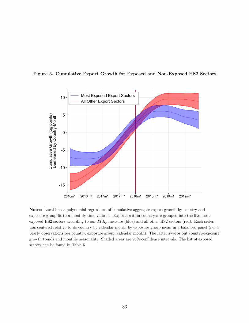
Figure 3. Cumulative Export Growth for Exposed and Non-Exposed HS2 Sectors

-15

-10

-5

0

5

10

Cum

ulat

ive

Gro

wth

(log

poi

nts)

Dem

eane

d by

Cou

ntry

-Mon

th

2016m1 2016m7 2017m1 2017m7 2018m1 2018m7 2019m1 2019m7

Most Exposed Export SectorsAll Other Export Sectors

Notes: Local linear polynomial regressions of cumulative aggregate export growth by country and

exposure group fit to a monthly time variable. Exports within country are grouped into the five most

exposed HS2 sectors according to our ITEp measure (blue) and all other HS2 sectors (red). Each series

was centered relative to its country by calendar month by exposure group mean in a balanced panel (i.e. 4

yearly observations per country, exposure group, calendar month). The latter sweeps out country-exposure

growth trends and monthly seasonality. Shaded areas are 95% confidence intervals. The list of exposed

sectors can be found in Table 5.

33

Figure 4. Ad Valorem Equivalent Tariff Change on U.S. Export Growth of ImportTariff Exposure

2019Effect

2018Effect

Mean +1 SD +2 SD0

.5

1

1.5

2

2.5

3

3.5

4

4.5

Ad V

alor

em E

quiv

. Tar

iff C

hang

e (%

Pts

)

0 .05 .1 .15 .2 .25 .3 .35Import Tariff Exposure of Exporters (ITE)

Notes: We compute the ad valorem equivalent tariff (AVE) using the coefficients in Table 10 and

equation (8). We average coefficients across quarters from 2018 and 2019.

34

Table 1. 2018 Tariff Incidence by 2016 Trade Patterns

Imports Exports

Share of Value 11.5 7.9

Share of Firms 32.9 18.7

Share of Employees 31.8 23.2

Tariffed Share at Affected Firms 46.5 32.5

Notes: “Imports” (“Exports”) show statistics for all importers (exporters) impacted by U.S.-imposedimport (foreign retaliatory export) tariffs. “Value” is the share of trade impacted by tariffs; “Firms” isthe share of firms affected by tariffs; “Share of Employees” is the share of private, non-farm employeesworking at affected firms, and “Tariffed Share at Affected Firms” is average trade value at affectedfirms that face tariffs.Source: Authors’ calculations using 2016 LFTTD.

Table 2. Average characteristics of firms affectedby new tariffs in 2018-2019

Panel A: Importers

Tariffed Importers All Importers All Firms

Employment 430.9 212 24.0

Establishments 9.3 4.8 1.3

Age 17.6 18.0 14.1

Pay/Worker ($1000s) 57.8 57.5 29.5

Panel B: Exporters

Tariffed Exporters All Exporters All Firms

Employment 720.3 241.7 24.0

Establishments 14.8 5.8 1.3

Age 22.5 18.8 14.1

Pay/Worker ($1000s) 64.2 57.1 29.6

Notes: Average firm characteristics by firm sample in top row of Panel A and B. Annual pay perworker in thousands of dollars. All firm details are based on 2016 firm-level data, the latest year avail-able.Source: Authors’ calculations using 2016 LFTTD and LBD.

35

Table 3. Tariff Incidence by Affected Sectors

Importers Exporters Implied DutiesEmployment Share Employment Share per Worker

Manufacturing 0.65 0.63 $1,595

Wholesale 0.51 0.38 $5,049

Retail 0.60 0.44 $364

Other 0.21 0.13 $314

Total 0.32 0.23 $893

Notes: Manufacturing is defined as all sectors within NAICS 31-33; Wholesale is defined as all sectorswithin NAICS 42; Retail is defined as all sectors within NAICS 44 and 45; and Other includes all othersectors except 92. Duty-per-worker weighted by sectoral employment. All calculations are based on2016 firm-level data, the latest year available. See text for futher details.Source: Authors’ calculations using 2016 LFTTD and LBD.

Table 4. Summary Statistics on Import Tariff Exposure

ITEBroadp ITEp ITENarrow

p

2016 0.545 0.111 0.050(0.127) (0.109) (0.063)

2014-2016 Average 0.526 0.105 0.047(0.125) (0.103) (0.060)

Tranche 1: Solar/Washing 0.060 0.001 0.0002(0.042) (0.012) (0.005)

Tranche 2: Metals 0.209 0.006 0.003(0.113) (0.041) (0.022)

Tranche 3: China 0.527 0.104 0.047(0.125) (0.107) (0.062)

Notes: This table displays means and standard deviations in parentheses of the three ITE measuresdescribed in Section 3 for our regression sample. The first row displays statistics for ITE measuresconstructed using 2016 data. The second row displays statistics for ITE measures constructed usingdata averaged over 2014-2016. Rows three through five, display statistics for ITE measures by thethree main tranches of tariffs using 2016 data. Tranche 1 refers solar products and washing machinestariffs; Tranche 2 refers to aluminum and steel tariffs; and Tranche 3 refers to tariffs on goods originat-ing in China.Source: Authors’ calculations using 2014-2016 LFTTD.

36

Table 5. Export Sectors that are the Most and Least Exposed to Import Tariffs

Panel A: Most Exposed

HS2 Product Description

29 Organic chemicals

85 Electrical machinery and equipment and parts thereof

72 Iron and steel

84 Nuclear reactors, boilers, machinery and mechanical appliances

73 Articles of iron or steel

Panel B: Least Exposed

HS2 Product Description

67 Prepared feathers/down; artificial flowers; articles of human hair

14 Vegetable plaiting materials

27 Mineral fuels, mineral oils and products of their distillation

47 Pulp of wood or of other fibrous cellulosic material

23 Residues from food industry, animal fodder, offal

Notes: This table reports the five most and five least exposed HS2 product categories with respectto the 2018-2019 import tariffs. HS2 sectors are ranked by the total number of HS6 products with anITEp measure greater than the 75th percentile of the overall ITEp distribution. Disclosure avoidanceprotocols preclude releasing a full ranking.Source: Authors’ calculations from 2016 LFTTD.

Table 6. Export Growth and Import Tariff Exposure

(1) (2) (3)

∆ ln(1 + τpct) -0.910*** -0.895*** -0.922***(0.124) (0.143) (0.121)

ITEp × I(> 2017Q4) -0.046** -0.045** -0.092***(0.022) (0.022) (0.025)

Fixed Effects ct, pq ct, pq, cI ct, pq, cI, ItObservations 4,208,229 4,208,226 4,208,226

Notes: * p<10%; ** p<5%; *** p<1%. Robust standard errors in parentheses, clustered by HS6product. The ITE measure is generated using data from the 2016 LFTTD. Fixed effects denotedby country (c), month (t), and HS section (I) and their interactions. All specifications include HS6-calendar quarter (pq) fixed effects.

37

Table 7. Export Growth and Import Tariff Exposure – Narrow, Baseline, and BroadMeasures

(1) (2) (3)

∆ ln(1 + τpct) -0.922*** -0.929*** -0.923***(0.121) (0.121) (0.121)

ITEp × I(> 2017Q4) -0.092***(0.017)

ITEBroadp × I(> 2017Q4) -0.097***

(0.025)

ITENarrowp × I(> 2017Q4) -0.123***

(0.039)

Fixed Effects ct, pq, cI, It ct, pq, cI, It ct, pq, cI, ItObservations 4,208,226 4,208,226 4,208,226

Notes: * p<10%; ** p<5%; *** p<1%. Robust standard errors in parentheses, clustered by HS6product. The ITE measures are generated using data from the 2016 LFTTD. Fixed effects denotedby country (c), month (t), and HS section (I) and their interactions. All specifications include HS6-calendar quarter (pq) fixed effects.

Table 8. Export Growth and Import Tariff ExposurePre-Tariff Period

(1) (2) (3)

∆ ln(1 + τpct) - - -

ITEp × I(> 2016Q4) 0.046(0.035)

ITEBroadp × I(> 2016Q4) 0.039

(0.057)ITENarrowp × I(> 2016Q4) 0.009

(0.037)

Fixed Effects ct, pq, cI, It ct, pq, cI, It ct, pq, cI, ItObservations 2,111,899 2,111,899 2,111,899

Notes: * p<10%; ** p<5%; *** p<1%. Robust standard errors in parentheses, clustered by HS6product. The ITE measures are generated using data from the 2016 LFTTD. Fixed effects denotedby country (c), month (t), and HS section (I) and their interactions. All specifications include HS6-calendar quarter (pq) fixed effects.

38

Table 9. Export Growth and Import Tariff Exposure by Tariff Tranche

ITEp ITEBroadp ITENarrowp

∆ ln(1 + τpct) -0.913*** -0.938*** -0.915***(0.120) (0.120) (0.121)

Interacted VariableT1× I(> 2017Q4) -0.702*** -0.222*** -0.903***

(0.150) (0.084) (0.115)

T2× I(> 2017Q4) -0.188** 0.085** -0.268**(0.081) (0.038) (0.128)

T3× I(> 2017Q4) -0.070** -0.083*** -0.105***(0.025) (0.029) (0.040)

Fixed Effects ct, pq, cI, It ct, pq, cI, It ct, pq, cI, ItObservations 4,208,226 4,208,226 4,208,226

Notes: * p<10%; ** p<5%; *** p<1%. Robust standard errors in parentheses, clustered by HS6product. The ITE measures are generated using data from the 2016 LFTTD. T1 refers to the respec-tive ITEp measure using only the import tariffs on washing machines and solar products; T2 refers tothe ITEp measure using only the import tariffs on steel and aluminum; and T3 to the ITEp measureusing only the import tariffs on goods from China. Fixed effects denoted by country (c), month (t),and HS section (I) and their interactions. All specifications include HS6-calendar quarter (pq) fixedeffects.

39

Table 10. Export Growth and Import Tariff Exposure, Quarterly Effects

(1) (2) (3)

ITEp ITENarrowp ITEBroadp

∆ ln(1 + τpct) -0.922*** -0.920*** -0.930***(0.121) (0.121) (0.121)

ITE (column variable)×Quarterly Indicator

×2018Q1 -0.049 -0.064* -0.81*(0.045) (0.069) (0.046)

×2018Q2 -0.049 -0.045 -0.107**(0.045) (0.069) (0.045)

×2018Q3 -0.077* -0.143** -0.081*(0.045) (0.071) (0.047)

×2018Q4 -0.097** -0.162** -0.074(0.047) (0.072) (0.047)

×2019Q1 -0.074* -0.107 -0.118***(0.043) (0.069) (0.040)

×2019Q2 -0.127*** -0.149** -0.150***(0.042) (0.067) (0.042)

×2019Q3 -0.185*** -0.254*** -0.153***(0.043) (0.066) (0.043)

×2019Q4 -0.077* -0.061 -0.016(0.044) (0.069) (0.045)

Fixed Effects ct, pq, cI, It ct, pq, cI, It ct, pq, cI, ItObservations 4,208,226 4,208,226 4,208,226

Notes: * p<10%; ** p<5%; *** p<1%. The regressions in this table are generated according to Equa-tion (7). Robust standard errors in parentheses, clustered by HS6 product. The ITE measures aregenerated using data from the 2016 LFTTD. Fixed effects denoted by country (c), month (t), and HSsection (I) and their interactions. All specifications include HS6-calendar quarter (pq) fixed effects.

40

Table 11. Export Growth and Import Tariff Exposure:Decomposition of Supply Chain Margins

(1) (2) (3) (4) (5)Baseline Broad Net Narrow Broad Net Fully

Baseline Narrow Decomposed

∆ ln(1 + τpct) -0.916*** -0.927*** -0.923*** -0.927*** -0.926***(0.120) (0.121) (0.121) (0.121) (0.121)

ITEp × I(> 2018Q3) -0.089*** -0.128***(0.026) (0.031)

ITENarrowp × I(> 2018Q3) -0.118*** -0.152*** -0.143***

(0.040) (0.042) (0.043)Broad Exposure Net of Baseline

[ITEBroadp − ITEp]× I(> 2018Q3) -0.083*** -0.083***

(0.029) (0.029)Broad Exposure Net of Narrow

[ITEBroadp − ITENarrowp ]× I(> 2018Q3) -0.091***

(0.027)Baseline Exposure Net of Narrow

[ITEp − ITENarrowp ]× I(> 2018Q3) -0.116***

(0.040)

Fixed Effects ct, pq, cI, It ct, pq, cI, It ct, pq, cI, It ct, pq, cI, It ct, pq, cI, ItObservations 4,208,226 4,208,226 4,208,226 4,208,226 4,208,226

Notes: * p<10%; ** p<5%; *** p<1%. Robust standard errors in parentheses, clustered by HS6product. The ITE measures are generated using data from the 2016 LFTTD. The decompositionregressions in columns (2), (4), and (5) are generated according to (9a) through (9c). Fixed effectsdenoted by country (c), month (t), and HS section (I) and their interactions. All specifications includeHS6-calendar quarter (pq) fixed effects.

41

Table 12. Export Growth and Import Tariff Exposure, Compare ITE Measures

(1) (2) (3)

∆ ln(1 + τpct) -0.922*** -0.929*** -0.923***(0.121) (0.121) (0.121)

ITEp × I(> 2017Q4) -0.102***(0.026)

ITEBroadp × I(> 2017Q4) -0.109***

(0.026)

ITENarrowp × I(> 2017Q4) -0.136***

(0.041)

Fixed Effects ct, pq, cI, It ct, pq, cI, It ct, pq, cI, ItObservations 4,208,226 4,208,226 4,208,226

Notes: * p<10%; ** p<5%; *** p<1%. Robust standard errors in parentheses, clustered by HS6product. Average ITE measures are generated using LFTTD data from 2014 through 2016. Fixedeffects denoted by country (c), month (t), and HS section (I) and their interactions. All specificationsinclude HS6-calendar quarter (pq) fixed effects.

42

Table 13. Export Growth and Import Tariff Exposure, Quarterly Effects, AverageITE

(1) (2) (3)

ITEp ITEBroadp ITE

Narrowp

∆ ln(1 + τpct) -0.922*** -0.930*** -0.920***(0.121) (0.121) (0.121)

ITE (column variable)×Quarterly Indicator

×2018Q1 -0.049 -0.88* -0.077(0.047) (0.046) (0.073)

×2018Q2 -0.060 -0.131*** -0.061(0.047) (0.046) (0.071)

×2018Q3 -0.081* -0.143** -0.170**(0.047) (0.048) (0.074)

×2018Q4 -0.123** -0.200*** -0.162**(0.049) (0.048) (0.075)

×2019Q1 -0.078* -0.112*** -0.126*(0.045) (0.041) (0.073)

×2019Q2 -0.140*** -0.150*** -0.151**(0.044) (0.043) (0.070)

×2019Q3 -0.200*** -0.166*** -0.250***(0.044) (0.044) (0.069)

×2019Q4 -0.087* -0.036 -0.055(0.046) (0.047) (0.072)

Fixed Effects ct, pq, cI, It ct, pq, cI, It ct, pq, cI, ItObservations 4,208,226 4,208,226 4,208,226

Notes: * p<10%; ** p<5%; *** p<1%. Robust standard errors in parentheses, clustered by HS6product. Average ITE measures are generated using LFTTD data from 2014 through 2016. Fixedeffects denoted by country (c), month (t), and HS section (I) and their interactions. All specificationsinclude HS6-calendar quarter (pq) fixed effects.

43

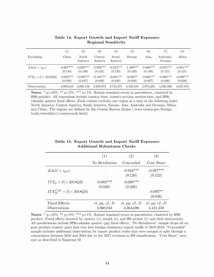
Table 14. Export Growth and Import Tariff Exposure:Regional Sensitivity

(1) (2) (3) (4) (5) (6) (7) (8)

Excluding: China North Central South Europe Asia Australia/ AfricaAmerica America America Oceania

∆ ln(1 + τpct) -0.967*** -0.695*** -0.902*** -0.912*** -1.409*** -0.980*** -0.925*** -0.921***(0.134) (0.130) (0.124) (0.120) (0.159) (0.136) (0.121) (0.121)

ITEp × I(> 2018Q3) -0.094*** -0.089*** -0.108*** -0.085*** -0.088** -0.066*** -0.086*** -0.090***(0.026) (0.027) (0.029) (0.026) (0.028) (0.027) (0.026) (0.026)

Observations 4,093,618 4,005,156 3,338,972 3,743,375 3,102,584 2,975,285 4,046,500 4,037,073

Notes: * p<10%; ** p<5%; *** p<1%. Robust standard errors in parentheses, clustered byHS6 product. All regressions include country-time, country-section, section-time, and HS6-calendar quarter fixed effects. Each column excludes one region at a time in the following order:North America, Central America, South America, Europe, Asia, Australia and Oceania, Africa,and China. The regions are defined by the Census Bureau (https://www.census.gov/foreign-trade/schedules/c/countrycode.html).

Table 15. Export Growth and Import Tariff Exposure:Additional Robustness Checks

(1) (2) (3)

No Retaliation Concorded Cost Share

∆ ln(1 + τpct) – -0.916*** -0.957***(0.120) (0.122)

ITEp × I(> 2018Q3) -0.082*** -0.089***(0.026) (0.026)

ITECostpc × I(> 2018Q3) -0.097**

(0.046)

Fixed Effects ct, pq, cI, It ct, pq, cI, It ct, pq, cI, ItObservations 4,060,043 4,304,696 4,131,358

Notes: * p<10%; ** p<5%; *** p<1%. Robust standard errors in parentheses, clustered by HS6product. Fixed effects denoted by country (c), month (t), and HS section (I) and their interactions.All specifications include HS6-calendar quarter (pq) fixed effects. “No Retaliation” sample drops all ex-port product-country pairs that ever face foreign retaliatory export tariffs in 2018-2019; “Concorded”sample includes additional observations for export product codes that were merged or split through aconcordance between 2016 and 2018 due to the 2017 revisions to HS classification. “Cost Share” mea-sure as described in Equation 10.

44

A Data Appendix

Export Data We employ monthly, public-use U.S. export data provided by the U.S.Census Bureau from 2015 to 2019. This data spans a major revision of the HS nomenclaturein 2017. To construct time consistent export flows at the 6-digit product level, we concorddata from 2017-2019 back to the 2012 revision of the HS using concordances from the UNStatistics Division.

Our baseline sample excludes the products that undergo any merging or splitting ofcodes. Note, we do not simply merge the data over time and keep unchanged codes. Some6-digit product codes from a prior revision may continue to be reused in subsequent revisions,but they might be aggregated or split in new ways. We keep track of the codes that undergoany revision where we have to aggregate for consistency. We check the robustness of ourmain result to adding or dropping these codes in Section 4.5.

Firm-Level Data Details of U.S. firm-level data are described in Section 2.2.

Import Tariff Data We collected data at the 8-digit tariff line level on new tariffs leviedby the U.S. from 2018-2019 as part of Sections 201, 232, and 301 investigations.

• Section 201: Solar Products, January 23, 2018. We use the list of products and countryexemptions from Presidential Proclamation 9693 (Federal Register, Vol 83, p. 3541)of January 23, 2018.

• Section 201: Washing Machines, January 23, 2018. We use the list of products andcountry exemptions from Presidential Proclamation 9694 (Federal Register, Vol 83, p.3553).

• Section 232: Steel and Aluminum, March 8, 2018 with subsequent waves adding ordropping countries (see Figure 2). These include the products listed in the Annexes toPresidential Proclamation 9704 (Federal Register, Vol. 83, p. 11619) and PresidentialProclamation 9705 (Federal Register, Vol. 83, p. 11625).

• Section 301: China, wave 1 (July 6, 2018), wave 2 (August 23,2018), and wave 3(September 24, 2018 and escalated on May 23, 2019). There are many modificationsand changes, especially to wave 3, where products are added and removed from earlierannexes in a series of Federal Register notices. We use an official list provided by theUSITC (https://hts.usitc.gov/view/China%20Tariffs?release=2019HTSARev20, accessed 1/30/2020).43

Export Retaliation Tariff Data Lists of new retaliatory tariffs levied against U.S. ex-ports by various countries is gathered from destination country sources, following information

43There are some duties levied at the HS 10-digit level against China, which we aggregated to the HS8-digit level.

45

produced for the trade war timeline in Bown and Kolb (2019). Since HS6 is the most dis-aggregated product category that is consistent across countries, we aggregate these lists tothe HS 6-digit level. Tariffs are associated with the month in which they were imposed. Thetotal amount of trade subject to retaliatory tariffs is computed using U.S. export data atthe HS 6-digit level in 2017. We include the following retaliation actions:

• Canada, July 2018: Retaliatory tariffs on $17.8 billion of U.S. exports. Information onthe products facing retaliation (”June 29 list”) accessed at https://www.piie.com/system/files/documents/bown-2018-07-05.xlsx.

• China, April 2018: Retaliatory tariffs on $2.4 billion of U.S. exports. Raw list ofcategories accessed at: http://images.mofcom.gov.cn/www/201803/201803260859

59196.pdf, with additional information here: https://piie.com/system/files/do

cuments/2018-04-09-piie-chart-lu-schott.xlsx.

• China, July 2018. Retaliatory tariffs on $29.2 billion of U.S. exports. Information onproducts facing retaliation (“Tariffs effective July 6”) accessed at: https://www.piie.com/system/files/documents/bown-2018-06-22.xlsx

• China, August 2018. Retaliatory tariffs on $15.3 billion of U.S. exports. Informationon products facing retaliation accessed at: http://images.mofcom.gov.cn/www/201

808/20180808201049842.pdf.

• China, September 2019: Retaliatory tariffs on $51.3 billion of U.S. exports. Informationon products facing retaliation (”Figure 2”) accessed at: https://www.piie.com/sys

tem/files/documents/bown2018-09-20.zip.

• China, June 2019: Retaliatory tariffs on $39.8 billion of U.S. exports. Information onproducts facing retaliation (”China Tariff Rates”, Column M) accessed at: https:

//www.piie.com/system/files/documents/bown-jung-zhang-2019-06-12.xlsx.

• European Union, June 2018: Retaliatory tariffs on $4.2 billion of U.S. exports. Infor-mation on the products facing “immediate retaliation” accessed at https://www.pi

ie.com/system/files/documents/bown-2018-06-29.xlsx.

• India, June 2019: Retaliatory tariffs on $1.3 billion of U.S. exports. List of affectedproducts accessed at https://docs.wto.org/dol2fe/Pages/FE Search/FE S S009-

DP.aspx?language=E&CatalogueIdList=246009,245254&CurrentCatalogueIdIndex=0&FullTextHash=371857150&HasEnglishRecord=True&HasFrenchRecord=Tru

e&HasSpanishRecord=True.

• Mexico, June 2018: Retaliatory tariffs on $4.5 billion of U.S. exports. Information onthe products facing retaliation (group 2) accessed at http://www.dof.gob.mx/nota d

etalle.php?codigo=5525036&fecha=05/06/2018.

• Turkey, May 2018: Retaliatory tariffs on $1.6 billion of U.S. exports. Information onthe products facing retaliation accessed at https://docs.wto.org/dol2fe/Pages/

FE Search/FE S S009-DP.aspx?language=E&CatalogueIdList=245272&CurrentCa

46

talogueIdIndex=0&FullTextHash=371857150&HasEnglishRecord=True&HasFrench

Record=False&HasSpanishRecord=True.

• Turkey, August 2018: Retaliatory tariffs on $1.6 billion of U.S. exports. List is identicalto May 2018 list, but rates are increased by different amounts. Information on theproducts facing retaliation accessed at https://www.resmigazete.gov.tr/eskiler

/2018/08/20180815-6.pdf.

B Empirical Aggregation to Export Growth

To fix ideas, we write down a simple empirical model where exporters may have been affectedby import tariffs. We index firms by i and products by p. Exporters with positive tradeto country c in product p are in the set Ωpc. Firm level export sales in product code p tocountry c in the absence of import tariffs are given by ripct. We define an indicator variableDit = 1 if any imports of firm i are hit by a new tariff and zero otherwise. We assume thatthe impact of the import tariff on a firm’s export output is potentially heterogeneous andadjusts output by 1− δip ≤ 1. We can interpret δip ∈ [0, 1] as a firm-product specific exporttrade friction induced by tariffs on its own imports.44

For clarity, we drop the product subscript and write observed exports rict of any firm tocountry c as,

rict = [(1−Dit) +Dit (1− δi)] rict = rict [1−Dδi] .

Note that unobserved firm-level exports in the absence of the tariff are rict. We aggregateover all exporters to obtain the equation for observable aggregate exports to country c

Rct =∑i∈Ωc

[1−Ditδi] rict

= Rct −∑i∈Ωc

Ditδirict

= Rct

[1−

∑i∈Ωc

Ditδirict

Rct

]= Rict

[1− δ

]The last line uses that

[1− δ

]is a trade weighted average of the heterogeneous export effect

of import tariffs on affected firms.We predict δi ∈ [0, 1] so that exports are possibly lower if firms imports are hit by new

tariffs, i.e.[1− δ

]< 1. We cannot do this directly because of unobserved heterogeneity of

impact across firms and because exports without the presence of tariffs rict in the weights

44The restriction to [0, 1] is a testable assumption. It is feasible that firms hit by an import tariff increasetheir output.

47

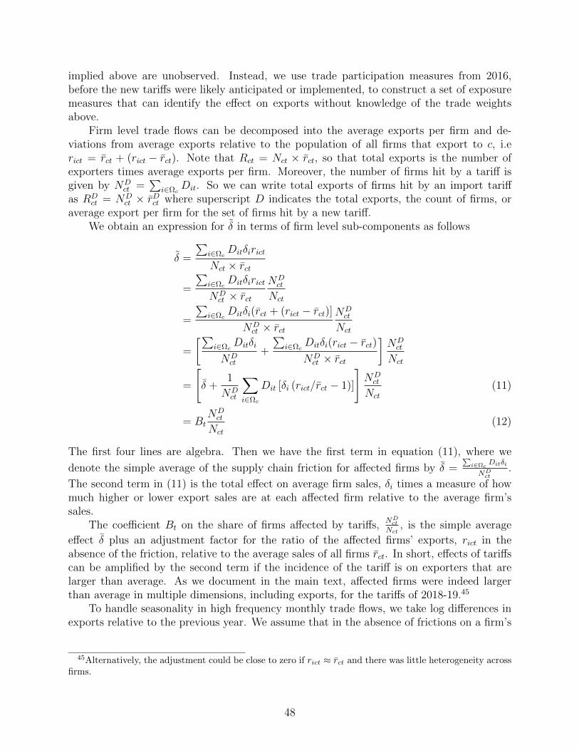
implied above are unobserved. Instead, we use trade participation measures from 2016,before the new tariffs were likely anticipated or implemented, to construct a set of exposuremeasures that can identify the effect on exports without knowledge of the trade weightsabove.

Firm level trade flows can be decomposed into the average exports per firm and de-viations from average exports relative to the population of all firms that export to c, i.erict = rct + (rict − rct). Note that Rct = Nct × rct, so that total exports is the number ofexporters times average exports per firm. Moreover, the number of firms hit by a tariff isgiven by ND

ct =∑

i∈ΩcDit. So we can write total exports of firms hit by an import tariff

as RDct = ND

ct × rDct where superscript D indicates the total exports, the count of firms, oraverage export per firm for the set of firms hit by a new tariff.

We obtain an expression for δ in terms of firm level sub-components as follows

δ =

∑i∈Ωc

Ditδirict

Nct × rct

=

∑i∈Ωc

Ditδirict

NDct × rct

NDct

Nct

=

∑i∈Ωc

Ditδi(rct + (rict − rct)]NDct × rct

NDct

Nct

=

[∑i∈Ωc

Ditδi

NDct

+

∑i∈Ωc

Ditδi(rict − rct)NDct × rct

]NDct

Nct

=

[δ +

1

NDct

∑i∈Ωc

Dit [δi (rict/rct − 1)]

]NDct

Nct

(11)

= BtNDct

Nct

(12)

The first four lines are algebra. Then we have the first term in equation (11), where we

denote the simple average of the supply chain friction for affected firms by δ =∑

i∈ΩcDitδi

NDct

.

The second term in (11) is the total effect on average firm sales, δi times a measure of howmuch higher or lower export sales are at each affected firm relative to the average firm’ssales.

The coefficient Bt on the share of firms affected by tariffs,ND

ct

Nct, is the simple average

effect δ plus an adjustment factor for the ratio of the affected firms’ exports, rict in theabsence of the friction, relative to the average sales of all firms rct. In short, effects of tariffscan be amplified by the second term if the incidence of the tariff is on exporters that arelarger than average. As we document in the main text, affected firms were indeed largerthan average in multiple dimensions, including exports, for the tariffs of 2018-19.45

To handle seasonality in high frequency monthly trade flows, we take log differences inexports relative to the previous year. We assume that in the absence of frictions on a firm’s

45Alternatively, the adjustment could be close to zero if rict ≈ rct and there was little heterogeneity acrossfirms.

48

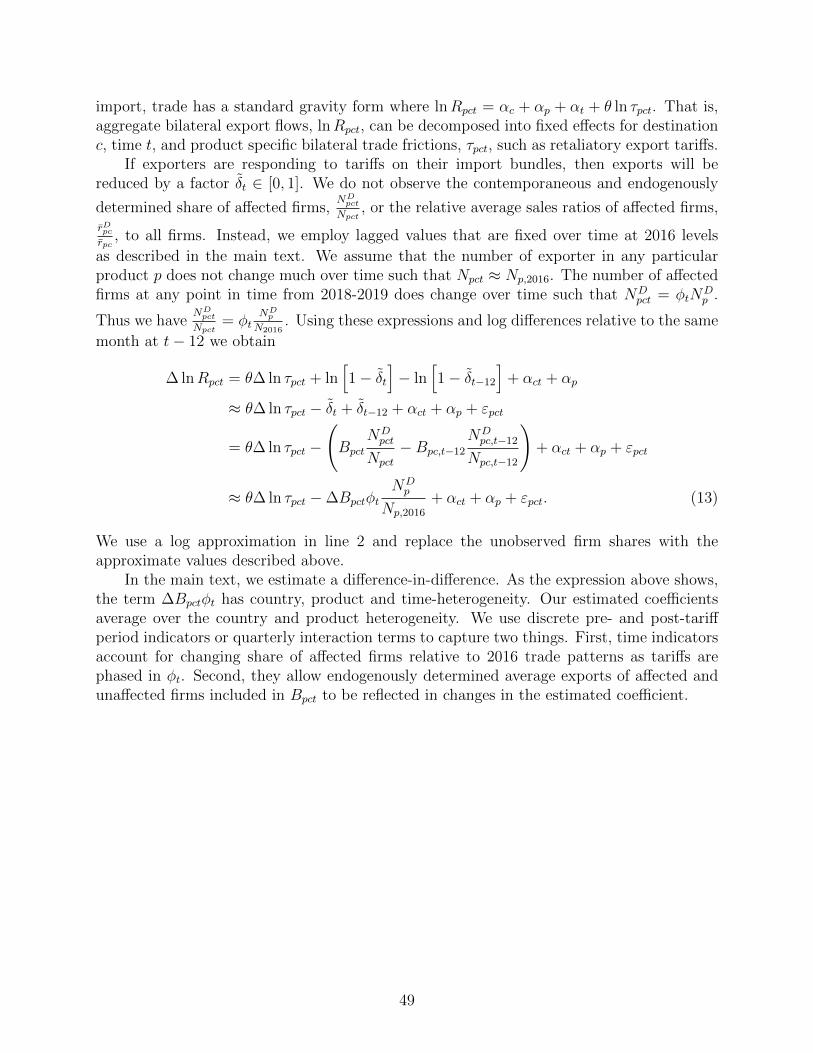
import, trade has a standard gravity form where lnRpct = αc + αp + αt + θ ln τpct. That is,aggregate bilateral export flows, lnRpct, can be decomposed into fixed effects for destinationc, time t, and product specific bilateral trade frictions, τpct, such as retaliatory export tariffs.

If exporters are responding to tariffs on their import bundles, then exports will bereduced by a factor δt ∈ [0, 1]. We do not observe the contemporaneous and endogenously

determined share of affected firms,ND

pct

Npct, or the relative average sales ratios of affected firms,

rDpcrpc

, to all firms. Instead, we employ lagged values that are fixed over time at 2016 levels

as described in the main text. We assume that the number of exporter in any particularproduct p does not change much over time such that Npct ≈ Np,2016. The number of affectedfirms at any point in time from 2018-2019 does change over time such that ND

pct = φtNDp .

Thus we haveND

pct

Npct= φt

NDp

N2016. Using these expressions and log differences relative to the same

month at t− 12 we obtain

∆ lnRpct = θ∆ ln τpct + ln[1− δt

]− ln

[1− δt−12

]+ αct + αp

≈ θ∆ ln τpct − δt + δt−12 + αct + αp + εpct

= θ∆ ln τpct −

(Bpct

NDpct

Npct

−Bpc,t−12

NDpc,t−12

Npc,t−12

)+ αct + αp + εpct

≈ θ∆ ln τpct −∆BpctφtNDp

Np,2016

+ αct + αp + εpct. (13)

We use a log approximation in line 2 and replace the unobserved firm shares with theapproximate values described above.

In the main text, we estimate a difference-in-difference. As the expression above shows,the term ∆Bpctφt has country, product and time-heterogeneity. Our estimated coefficientsaverage over the country and product heterogeneity. We use discrete pre- and post-tariffperiod indicators or quarterly interaction terms to capture two things. First, time indicatorsaccount for changing share of affected firms relative to 2016 trade patterns as tariffs arephased in φt. Second, they allow endogenously determined average exports of affected andunaffected firms included in Bpct to be reflected in changes in the estimated coefficient.

49

Table A-1. Exporters Paying Import Tariffs: Supply Chain Incidence

Relationship between exported and imported tariffed product:

Any Product Same HS4 Same HS6Broad Baseline Narrow

(1) (2) (3)

Share of Exports 84% 43% 30%

Share of Exporters 24% 13% 11%

Notes: “Broad” considers exports of all firms that import at least one product subject to import tar-iffs. “Baseline” considers firm exports in a HS6 category that shares the same HS4 as firm importssubject to import tariffs. “Narrow” considers only those exports in the same HS6 category as firm im-ports subject to import tariffs.Source: Authors’ calculations using 2016 LFTTD.

Table A-2. Summary Statistics: Import Tariff Exposure and U.S. Export Growth

Mean St.Dev.

∆lnExportspct -.0023 1.27

Foreign Retaliation ∆ln(1 + τpct)

Full Sample (with zeros) 0.0014 0.015Tariff Increases 0.13 0.07

Import Tariff Exposure

ITEp 0.11 0.11

ITEBroadp 0.55 0.13

ITENarrowp 0.05 0.06

Notes: ITE measures described in Section 3.Source: Authors’ calculations using 2016 LFTTD, public-use Census Bureau data on U.S. monthlyexports. Conditional on a tariff increase for a country-product-month triplet, there are about 46,000observations, or about 1% of the sample.

50

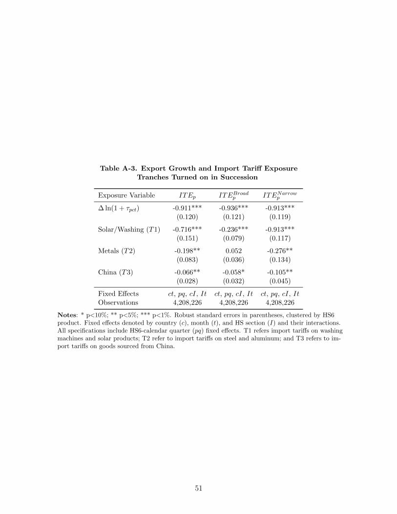
Table A-3. Export Growth and Import Tariff ExposureTranches Turned on in Succession

Exposure Variable ITEp ITEBroadp ITENarrowp

∆ ln(1 + τpct) -0.911*** -0.936*** -0.913***(0.120) (0.121) (0.119)

Solar/Washing (T1) -0.716*** -0.236*** -0.913***(0.151) (0.079) (0.117)

Metals (T2) -0.198** 0.052 -0.276**(0.083) (0.036) (0.134)

China (T3) -0.066** -0.058* -0.105**(0.028) (0.032) (0.045)

Fixed Effects ct, pq, cI, It ct, pq, cI, It ct, pq, cI, ItObservations 4,208,226 4,208,226 4,208,226

Notes: * p<10%; ** p<5%; *** p<1%. Robust standard errors in parentheses, clustered by HS6product. Fixed effects denoted by country (c), month (t), and HS section (I) and their interactions.All specifications include HS6-calendar quarter (pq) fixed effects. T1 refers import tariffs on washingmachines and solar products; T2 refer to import tariffs on steel and aluminum; and T3 refers to im-port tariffs on goods sourced from China.

51