NBER WORKING PAPER SERIES

WHEN ARE CONTRARIAN PROFITS DUE TOSTOCK MARKET OVERREACTION?

Andrew W. Lo

A Craig MacKinlay

Working Paper No. 2977

NATIONAL BUREAU OF ECONOMIC RESEARCH1050 Massachusetts Avenue

Cambridge, MA 02138May 1989

We thank Andy Abel, Mike Gibbons, Don Keim, Bruce Lehmann, Rob Stambaugh areferee, and seminar participants at Harvard University, University ofMaryland, University of Western Ontario, and the Wharton School for useful

suggestions and discussion. Research support from the Ceewax-Terker Research

Fund (MacKinlay), the National Science Foundation, the John M. OlinFellowship at the NEER (Lo), and the Q Group is gratefully acknowledged.This paper is part of NBER's research program in Financial Markets andMonetary Economics. Any opinions expressed are those of the authors notthose of the National Bureau of Economic Research.

NBER Working Paper p2977May 1989

WHEN ARE CONTRARIAN PROFITS DUE TOSTOCK MARKET OVERREACTION?

ABSTRACT

The profitability of contrarian investment strategies need not be the resultof stock mar-ket overreaction. Even if returns on individual securities are temporally independent,portfolio strategies that attempt to exploit return reversals may still earn positive ex-pected profits. This is due to the effects of cross-autocovariances fromwhich contrarianstrategies inadvertently benefit. We provide an informal taxonomy of return-generatingprocesses that yield positive [and negative expected profitsunder a particular contrar-ian portfolio strategy, and use this taxonomy to reconcile the empirical findings of weaknegative autocorrelation for returns on individual stocks with the strong positive auto-correlation of portfolio returns. We present empirical evidence against overreaction asthe primary source of contrarian profits, and show the presence of important lead—lagrelations across securities.

Andrew W. Lo A. Craig MacKinlaySloan School of Management Department of FinanceM.I.T. Wharton School50 Memorial Drive University of PennsylvaniaCambridge, MA 02139 Philadelphia, PA 19104

1. Introduction.

Since the publication of Louis Bachelier's thesis Theory of Speculation in 1900,

the theoretical and empirical implications of the random walk hypothesis as a modelfor speculative prices have been subjects of intense interest to financial economists.

Although first developed by Bachelier from rudimentary economic considerations of"fair games," the random walk has received broader support from the many earlyempirical studies confirming the unpredictability of stock price changes.1 Of course, it

is by now well-known that the unforecastability of asset returns is neither a necessary

nor a sufficient condition of economic equilibrium.2 And, in view of recent empirical

evidence, it is also apparent that historical stock market prices do not follow random

walks.3

This fact surprises many economists because the defining property of the randomwalk is the uncorrelatedness of its increments, and deviations from this hypothesis nec-essarily imply forecastable price changes.4 Several recent studies have attributed this

forecastability to what has come to be known as the "stock market overreaction" hy-

pothesis, the notion that investors are subject to waves of optimism and pessimism and

therefore create a kind of "momentum" which causes prices to temporarily swing away

from their fundamental values.5 Although such a hypothesis may be intuitively appeal-

ing, and does yield predictability since what goes down must come up and vice-versa,

a well-articulated equilibrium theory of overreaction with sharp empirical implications

has yet to be developed. But common to virtually all existing "theories" of over-reaction is one very specific empirical implication: price changes must be negativelyautocorrelated for some holding period.6 Therefore, the extent to which the data are

consistent with stock market overreaction, broadly defined, may be distilled into an

See, for example, the papers in Cootner (1964), and Fama (1965, 1970).21n particular, see Leroy (1973) and Lucas (1978).3See, for example, Lo and MacKinlay (1988). Our usage of the term "random walk" differs slightly from the classical

definition of a process with independently and identically distributed increments. We are interested primarily in theunconelatedneu of increment., and not in either independence or identically distributed innovations. Therefore, a processwith uncorrelated but heteroscedastic first-differences would fall into our definition of a random walk; see Lo and MacKinlay(1988) for the exact statement of the random walk hypothesis that we implicitly use here.

4flowever, our surprise must be tempered by the observation that forecasts of stock returns are still subject to randomfluctuations, so that profit opportunities are not immediate consequences of forecastability. Nevertheless, recent studiesmaintain the possibility of significant profits, even after controlling for risk in one way or another.

6For example, see DeBondt and Thaler (1985, 1987), Dc Long et. al. (1989), Lehmann (1988), Poterba and Summers(1988), and Shefrin and Statman (1985).

For example, DeBondt and Thaler (1985) write: "If stock prices systematically overshoot, then their reversal shouldbe predictable from past return data alone . . ." Other studies that consider overreaction also assume this either explicitlyor implicitly.

3.4 —1— 5.89

empirically decidable question: are return reversals responsible for the predictability

in stock returns?A more specific consequence of overreaction is the profitability of a contrarian

portfolio strategy, a strategy that exploits negative serial dependence in asset returns

in particular. The defining characteristic of a contrarian strategy is the purchase of

securities that have performed poorly in the past and the sale of securitiesthat have per-

formed well.7 Selling the "winners" and buying the "losers" will earn positive expected

profits because current losers are likely to become future winners and current winners

are likely to become future losers when stock returns are negatively autocorrelated.

Therefore, it may be said that an implication of stock market overreaction is positive

expected profits from a contrarian investment rule. It is the apparent profitabilityof several contrarian strategies that has led many to conclude that stock markets do

indeed overreact.In this paper we question the reverse implication that the profitability of contrar-

ian investment strategies is evidence of stock market overreaction. Whereas return

reversals may be sufficient to yield positive expected profits from a contrarian strat-

egy, they are not necessary. Indeed, as an illustrative example we construct a simple

return-generating process in which each security's return is temporally independent,

and yet will still yield positive expected profits for a portfolio strategy that buys losersand sells winners. This seemingly counterlntuitive result is a consequence of positivecross-cut ocovarsances across securities, from which contrarian portfolio strategies inad-

vertently benefit. For a single security in isolation, negative serial correlation is indeednecessary and sufficient for the contrarian investor to earn positive expected profits.

However, when there are many securities to choose from the complex cross-effectsamong the distinct assets break this link. Therefore, the fact that some contrarian

strategies have positive expected profits need not imply that stock markets overreact.

In fact, for the particular contrarian strategy we examine, over half of the expectedprofits is due to cross-effects and not to negative autocorrelation in individual security

returns.However, the most striking aspect of our empirical findings is that these cross-

effects are generally positive in sign and have a pronounced lead—lag structure: the

p.rformanc. I. d.fned and for whatlengthof tim. generates as many different kinds of contrarian strategies asthere ar theories of overreaction.

3.4 —2— 5.89

returns of large capitalization stocks almost always lead those of smaller stocks. This re-

sult, coupled with the observation that individual security returns are generally weakly

negatively autocorrelated, indicates that the recentlydocumented positive autocorrela-

tion in weekly returns indexes is completely attributable to cross-effects. By exploiting

our contrarian strategy framework, we show that these cross-autocorrelations are incon-

sistent with a return-generating process that is the sum of a positively autocorrelated

common factor [which generates positive index autocorrelation] plus an idiosyncratic

bid-ask spread process [which yields weak negative serial dependence in individual re-

turns]. Although this is a negative result, it does provides important guidance for

theoretical models of equilibrium asset prices attempting to explain positive index au-tocorrelation via time-varying conditional expected returns. Such theories must be

capable of generating lead—lag patterns, since it is the cross-autocorrelations that is

the source of positive dependence in stock returns.Since we focus only on the expected profits of the contrarian investment rule and

not on its risk, our results have implications for stock market efficiency only insofar as

they provide restrictions on economic models that might be consistent [or inconsistent]with the empirical results. We do not assert or deny the existence of "excessive"contrarian profits. Such an issue cannot be addressed without specifying an economic

paradigm within which asset prices are rationally determined in equilibrium.8 However,

we have found the contrarian investment strategy to be a convenient tool in exploring

the autocorrelation properties of stock returns. Moreover, our analysis of the natureof expected profits does point to more specific sources of risk for contrarian strategies

that must be weighed in assessing market efficiency. We leave this more ambitious task

to future research.In Section 2 we provide a summary of the autocorrelation properties of daily,

weekly and monthly returns, documenting the positive dependence in portfolio returnsand the negative autocorrelations of individual returns. Section 3 presents a formal

analysis of the expected profits from a specific contrarian investment strategy under

several different return-generating mechanisms, and shows how positive expected profits

need not be related to overreaction. In Section 4 we attempt to empirically quantifythe proportion of contrarian profits that may be attributed to overreaction and find

8Some have accounted for rick in one way or another with mixed result.. For example, Chan (1988) claims thatDeBondt and Thaler's (1985) excess profits are minimal after properly adjusting for risk, whereas Lehmann (1988) uses acontinuous-time argument to conclude that his weekly trading strategy is excessively profitable.

3.4 —3— 5.89

that a substantial portion cannot be. We show that a systematic lead—lag relation

among returns of size-sorted portfolios is the primary source of contrarian profits and

positive index autocorrelation. In Section 5 we provide some discussion of our useof

weekly returns in contrast to the much longer-horizon returns used in previous studiesof stock market overreaction, and we conclude in Section 6.

2. A Summary of Current Findings.

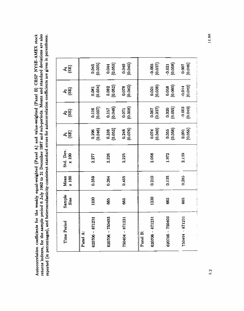
In Table la we report the first four autocorrelations of weekly equal-weighted andvalue-weighted returns indexes for the sample period from 6 July 1962 to 31 December

1987, where the indexes are constructed from the CRSP daily returns files.9 For thissample period the equal-weighted index has a first-order autocorrelation of approx-

imately 30 percent. Since its heteroscedasticity-consistent standard error is 0.046, thisautocorrelation is statistically different from zero at all conventional significance lev-els. The sub-period autocorrelations indicate that this significance is not an artifact of

any particularly influential sub-sample; equal-weighted returns are strongly positivelyautocorrelated throughout the sample. Higher order autocorrelations are also posi-tive although generally smaller in magnitude, and the decay rate is somewhat slowerthan the geometric rate of an AR(1) [for example, is 8.8 percent whereas /2 is 11.6

percentj.To develop a sense of the economic importance of the autocorrelations, recall that

the R2 of a regression of returns on a constant and its first lag is the square of the slope

coefficient which is simply the first-order autocorrelation. Therefore, an autocorrelation

of 30 percent implies that 9 percent of weekly return variation is predictable by using

only the preceding week's returns. In fact, the autocorrelation coefficients implicit inLo and MacKinlay's (1988) variance ratios are as high as 49 percent for a sub-sampleof the portfolio of stocks in the smallest size quintile, implying an R2 of about 25

percent. This degree of predictability suggests that a profitable trading strategy mightbe to switch from stocks to bonds when this week's predicted index return falls below

the risk-free rate, and vice-versa when it is above. With no transactions costs, theprofitability of such a trading rule may be readily verified.

Unles. stated otherwise we take returns to be simple returns and not continuously-compounded. Our conitniction ofweekly returns is described in Lo and MacKinlay (1988).

34 _4_. 5.89

It may therefore come as some surprise that individual returns are generally weakly

negatively autocorrelated. Table 2a reports the cross-sectional average of autocorrela-

tion coefficients across all stocks that have at least 52 non-missing weekly returns during

the sample period. For the entire cross-section of 4786 such stocks, the average first-

order autocorrelation coefficient, denoted by is —3.4 percent with a cross-sectional

standard deviation of 8.4 percent. Therefore, most of the individual first-order auto-correlations fall between —20 percent and 13 percent. This implies that most R2's ofregressions of individual security returns on their return last week fall between 0 and

4 percent, considerably less than the predictability of equal-weighted index returns.Average higher-order autocorrelations are also negative, though smaller in magnitude.The negativity of autocorrelations may be an indication of stock market overreaction

for individual stocks, but it is also consistent with the existence of a bid-ask spread.

We discuss this further in Section 3.

Table 2a also reports average autocorrelations within size-sorted quintiles.'° Thenegative autocorrelations are stronger in the smallest quintile but even the largestquintile has average autocorrelations less than zero. Compared to the 30 percent auto-

correlation of the equal-weighted index, the magnitudes of the individual autocorrela-

tions indicated by the means [and standard deviations] in Table 2a are generally much

smaller.

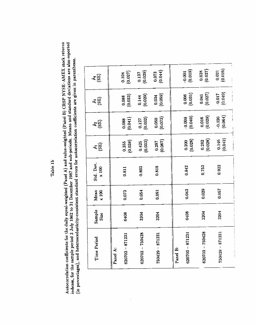
For completeness, we also report autocorrelations for returns on daily and monthly

indexes in Tables lb and ic; cross-sectional averages of autocorrelations for daily andmonthly returns on individual stocks are given in Tables 2b and 2c. Similar patternsare observed: autocorrelations are strongly positive for index returns [35.5 and 14.8

percent p31's for the equal-weighted daily and monthly indexes respectively], and weakly

negative for individual securities [—1.4 and —2.9 percent 3's for daily and monthly

returns respectively].The general tendency for individual security returns to be negatively serially de-

pendent and for portfolio returns such as those of the equal- and value-weighted market

to be positively autocorrelated raises an intriguing issue. We mentioned earlier thatbecause the equal-weighted index exhibits strong positive autocorrelation, a profitableinvestment strategy would be to allocate assets into equity when equity returns are high

'°AIl eiie-socted portfolio. are conitructed by .orting only once ueing market va1ue of equity at the middle of the.ample period], hence their compoeition doe. not change over time.

3.4 —5— 5.89

and into bonds when equity returns are low. This, however, is at odds with virtually

any contrarian strategy since it involves buying winners and selling losers. And yet

several contrarian strategies have also been shown to yield positive expected profits,'1

even though movements in the aggregate stock market do not support overreaction and

the returns of individual stocks are generally only marginally predictable. Is it possible

that contrarian profits are due to something other than overreacting investors? We

answer these questions in the next two sections.

3. Analysis of Contrarian Profitability.

To reconcile the profitability of contrarian investment strategies with the posi-

tive autocorrelation in stock returns indexes, we examine the expected profits of one

such strategy under various assumptions on the return-generating process. Consider a

collection of N securities and denote by Rt the Nxl—vector of their period t returns

• . . Ry]'. For convenience, we maintain the following assumption throughout this

section:

(Al) R is a jointly covariance-stationary stochastic process with expectation

E[R] = ••, N1' and autocovariance matrices E[(Rt.....k —— = r where, with no loss of generality, we take k � 0 since

rk = r'_k.12

In the spirit of virtually all contrarian investment strategies, consider buying stocks at

time t that were "losers" at time t —k and selling stocks at time t that were "winners"

at time t — k, where winning and losing is with respect to the equal-weighted returnon the market. More formally, if w2(k) denotes the fraction of the portfoliodevoted to

security i at time t, let:

"For .xaznpl., D.Bondt and Thaler (1985, 1987) and L.hmann (1988).t2Auuznption (Al) 1. made for notational simplicity, since joint covariance.stationaxity allows us to eliminate time-

indexes from population moments such as and re; th. qualitative features of our results will not change under theweaker assumptions of weakly dependest heterogeneously distributed vectors R,. This would merely require replacingexpectations with corresponding probability limits of suitably defined time-averages. For the results in this section, theadded generality does not outweigh the expoaltiorial complexity that a weakei set of assumptions requires. However, theempirical result, of Section 4 are based on these weaker assumptions; interested reader. may refer to conditions (A2)—(A4)in Appendix 2.

3.4 —6— 5.89

w2(k) = —(Rit_k

— Rmt_k) (3.1)

where R...k Rjtk/N is the equally-weighted market index.13 If, for example,

k = 1 then the portfolio strategy in period t is to short the winners and buys the losers

of the previous period, t — 1. By construction, t(k) [.i(k) w2t(k) •.. wNt(k)]' is

an arbitrage portfolio since the weights sum to zero. Therefore, the total investment

long [or short] at time t is given by It(k) where:

It(k) Iw2t(k)l . (3.2)

Since the portfolio weights are proportional to the differences between the marketindex and the returns, securities that deviate more positively from the market at timet — k will have greater negative weight in the time t portfolio, and vice-versa. Such a

strategy is designed to take advantage of stock market overreactions as characterized,

for example, by DeBondt and Thaler (1985): "(1) Extreme movements in stock prices

will be followed by extreme movements in the opposite direction. (2) The more extreme

the initial price movement, the greater will be the subsequent adjustment." The profit

ir(k) from such a strategy is simply:

N

irt(k) = w(k)Rjt . (3.3)

Re-arranging (3.3) and taking expectations yields the following:14

'3Thie is perhaps the simplest portfolio strategy that captures the essence of the contrarian principle. Lehmann (1988)also consaders this strategy, although he employs a more complicated strategy in his empirical analysis in which the portfolioweights (3.1) are re-normalised each period by a random factor of proportionality so that the investment is always onedollar long and short. This portfolio strategy is also similar to that of DeBondt and Thaler (1985 1987) although incontrast to our us of weekly returns they consider holding periods of three years. See Section 5 for further discussion.

"The relatively straightforward derivation of this equation is included in Appendix 1 for completeness. This is thepopulation counterpart of Lehmann's (1988) sample moment equation (5) divided by N.

3.4 —7— 5.89

E[irt(k)] = ____ — tr(1') —1

— )2 (34)

where sum = sit/N and tr(.) denotes the trace operator. The first term

of (3.4) is simply the k-th order autocovariance of the equally-weighted market index.

The second term is the cross-sectional average of the k-th order autocovariances of the

individual securities, and the third term is the cross-sectional variance of the mean

returns. Since this last term is independent of the autocovariances 1'k and does not

vary with k, we define the profitability index Lk = L(rk) and the constant a2() as:

____ — tr(rk)1

::(su — . (3.5)

thus,E[irt(k)1 = Lk — c2(su) . (3.6)

For purposes that will become evident below we re-write Lk as the following sum:

= [t'rt — tr(rjj} — (V 1) tr(rk) Ck + °k (3.7)

where:

Ck [t'rkt—tr(rk)J , — (N_i) .tr(rk) (3.8)

hence:

E(rt(k)] = Ck + °k — a2(su) . (3.9)

3.4 —8— 5.89

Written this way, it is apparent that expected profits may be decomposed into threeterms, one [Ck] depending on only the off-diagonals of the autocovariance matrix rk, the

second [Ok] depending on only the diagonals, and a third [c2(z)] which is independentof the autocovariances. This allows us to separate the fraction of expected profits due

to the cross-autocovariances Ck, versus the own-autocovariances °k of returns.

From (3.9), it is clear that the profitability of the contrarian strategy (3.1) maybe perfectly consistent with a positively autocorrelated market index and negativelyautocbrrelated individual security returns. Positive cross-autocovariances imply that

the term Ck is positive, and negative autocovariance for individual securities implies

that °k is also positive. Conversely, the empirical finding that equal-weighted indexesare strongly positively autocorrelated and that individual security returns are weakly

negatively serially dependent implies, through (3.7), that there must be significantpositive cross-autocorrelations across securities. To see this, observe that the first-

order autocorrelation of the equally-weighted index Rmt is simply:

Cov[R,,_1, RJ — _____ — tr(ri)+ tr(r1) 3 10

Var[R]— — .

The numerator of the second term of the right-hand side of (3.10) is simply the sum

of the first-order autocovariances of individual securities which, if negative, impliesthat the first term must be positive in order for the sum to be positive. Therefore,the positive autocorrelation in weekly returns may be attributed solely to the positivecross-autocorrelations across securities.

The expression for Lk also suggests that stock market overreaction need not be the

reason that contrarian investment strategies are profitable. To anticipate the examples

below, if returns are positively cross-autocorrelated then a return-reversal strategywill yield positive profits on average, even if individual security returns are temporally

independent! That is, if a high return for security A today implies that security B'sreturn will probably be high tomorrow, then a contrarian investment strategy will beprofitable even if each security's returns are unforecastable using past returns of thatsecurity only. The intuition for such a result is straightforward. Suppose there areonly the two stocks, A and B; if A's return is higher than the market today, we sell itand buy B. But if A and B are positively cross-autocorrelated, a higher return for A

3.4 —9-- 5.89

today implies a higher return for B tomorrow [on averages, thus we will have profited

from our long position in B [on average. Nowhere do we require that the stock market

overreacts, i.e., that individual returns are negatively autocorrelated. Of course, the

presence of stock market overreactions enhances the profitability of the return-reversal

strategy, but it is not necessary.To organize our understanding of the sources and nature of contrarian profits,

we provide four illustrative examples below. They are highly stylized special cases,nevertheless they yield a useful informal taxonomy of conditions necessary for the

average profitability of the investment strategy (3.1).

3.1. The I.LD. Benchmark.

Let returns Rt be both cross-sectionally and temporally independent. In this case

rk = 0 for all non-zero k hence:

Lk=Ck=Ok=O (3.11)

E[irt(k)] = — c2(j) < 0. (3.12)

Although returns are both temporally and cross-sectionally unforecastable, the ex-pected profits are negative as long as there is some cross-sectional variation in expected

returns. This is a result of the fact that our strategy is shorting the higher and buy-ing the lower mean return securities respectively, a losing proposition even when stock

market prices do follow random walks.15 Since o2(iz) is generally of small magnitude

and does not depend on the autocovariance structure of Rt, we will focus on Lk and

ignore o2(i) for the remainder of Section 3.

3.2. Stock Market Overreaction and Fads.

Almost any operational definition of stock market overreaction implies that indi-

vidual security returns are negatively autocorrelated over some holding period, so that

'This provides a simpi. count.rexaznpl. to th. somewhat surprising implication that on. cannot sy,tematicafly losemoney in th. stock market if price, follow random walks land there ar. no transactions costs). Multiple securities withdistinct mean. imply the exist.nc. of portfolio strategies with positive and negativ, expected returns.

3.4 — 10 — 5.89

"what goes up must come down" and vice-versa. If we denote by (k) the i,j-thelement of the autocovariance matrix rk, the overreaction hypothesis implies that the

diagonal elements of rk are negative, i.e., y(k) <0, at least for k = 1 when the span

of one period corresponds to a complete cycle ofoverreaction.'6 Since the overreaction

hypothesis generally does not restrict the cross-autocovariances, for simplicity we set

them to zero, i.e., -y3(k) = O,i j. Hence, we have:

-y,1(k) 0 ...

Fk = (y22(k)

) . (3.13)

0 0 '7NN(k)

The profitability index under these assumptions for R is then:

= = (N_l)t(r) = (N_1)(k) > 0 (3.14)

where the cross-autocovariance term Ck is zero; the positivity of Lk follows from thenegativity of the own-autocovariances, assuming N > 1. Not surprisingly, if stockmarkets do overreact the contrarian investment strategy is profitable on average.

Another price process for which the return-reversal strategy will yield positiveexpected profits is the sum of a random walk and an AR(1), which has been recently

proposed as a model of "fads" and "animal spirits."17 Specifically, let the dynamics

for the log-price X1 of each security i be given by:

= Y + Z (3.15)

where

= i + + Lt (3.16)

= pjZj.1 + z.' 0 <p < 1 (3.17)

We dicuu thu further in Sectio 5.'TSee for exarripte,. Summer, (I86).

3.4 — 11 — 5.89

and the disturbances {jt} and {i.'} are temporally, mutually, and cross-sectionallyindependent at all positive leads and lags.18 The k-th order autocovariance for the

return vector R is then given by the following diagonal matrix:

= diag [ _iP101 N'N ] . (3.18)

The profitability index follows immediately:

= = — (N_i) .tr(rk)N—i .p_1+;tc1 > 0 (3.19)

Since the own-autocovariances in (3.18) are all negative this is a special case of (3.13)

and may therefore be interpreted as an example of stock market overreaction. However,the fact that returns are negatively autocorrelated at all lags is an artifact of the first-order autoregressive process and need not be true for the sum of a random walk and a

general stationary process, a model that has been proposed for both stock market fads

and time-varying expected returns.'9 For example, let the "temporary" component of

(3.15) be given by the following stationary AR(2) process:

= z_1 — + zij . (3.20)

It is easily verified that the first-difference of Z is positively autocorrelated at lag 1implying that L1 < 0. Therefore, stock market overreaction necessarily implies the

profitability of the portfolio strategy (3.1) [in the absence of cross-autocorrelation[, butstock market fads do not.

"This last assumption requires only that e, is independent of c,.+.k for k 0. hence the disturbance, may be contem-poraneously cross-sectionally dependent without loss of generality.

'5For example, see Fazna and French (1988) and Summers (1986).

3.4 — 12 — 5.89

3.3. Trading on White Noise and Lead—Lag Relations.

Let the return-generating process for Rt be given by:

R.it = p + /31At_ + Et , f3 > 0 , (3.21)

where At is a temporally independent common factor with zero mean and variance

and the €t'5 are assumed to be both cross-sectionally and temporally independent.

These assumptions imply that for each security i, its returns are white noise with drift]

so that future returns to i are not forecastable from its past returns. This temporal

independence is certainly not consistent with either the spirit or form of the stock

market overreaction hypothesis. And yet it is possible to predict i's returns using past

returns of security j, where 5 < i. This is obviously an artifact of (3.21) in which the

return on the i-th security depends positively on a lagged common factor, where thelag is determined by the security's index. This implies that the return of security 1leads that of securities 2, 3, etc.; the return of security 2 leads that of securities 3,4, etc.; and so on. Alternatively, observing the return on security 1 today will help

forecast the return on security 2 tomorrow, but today's return on security 2 providesno information for how security 1 will fare tomorrow. This lead—lag relation will induce

positive expected profits for the contrarian strategy (3.1). To see this, observe that:

o /31/32 0 0 ... ()

o 0 /32/33 0 •.. 0

= : .. (3.22)

o o 0 0 ... 13N-113No 0 0 0" 00 0 /31/33 0 ... 00 0 0 132/34 0

I'2 = •..(3.23)0 0 0 0 13N—313N—100 0 0 000 0 0 0

3.4 — 13 — 5.89

and, more generally, when k < N then rk has zeros in all entries except along the

k-th super-diagonal, for which ji+k = cI3I3+k. For future reference, observe that acharacteristic of the lead—lag model is the asymmetry of the autocovariance matrix rk.

The profitability index in this case is:

I3I3+i > 0. (3.24)

From this example the importance of the cross-effects is evident; although each security

is individually unpredictable, a contrarian strategy may still profit if securities arepositively cross-correlated at various leads and lags. Moreover, it should be apparent

that less contrived return-generating processes will also yield posilive expected profitsto contrarian strategies as long as the cross-autocovariances are sufficiently large. One

source of such cross-effects may be non-synchronous trading, as in the models of Scholes

and Williams (1977) and Cohen et. a!. (1986). For example, the non-trading processproposed by Cohen et. a!. induces the following time series properties in observedreturns when true returns are generated by the market model:20

1. Individual returns are negatively autocorrelated.

2. A market index composed of observed returns to securities with positive betas will

exhibit positive serial dependence.

3. Cross autocorrelations of returns for securities i and j will be non-zero, and of the

same sign as f3f3.

If securities' betas are generally of the same sign, then non-trading induces positive

cross-effects; coupled with the negative individual autocorrelations, this yields positiveexpected profits for a contrarian investment strategy. However, Lo and MacKinlay(1989) show that the magnitudes of cross-effects documented in Section 4 cannot be

completely attributed to non-synchronous trading biases.

2o Chapter 6 of Cohen et. al. (1986).

3.4 — 14 — 5.89

3.4. A Positively Dependent Common Factor and the Bid-Ask Spread.

One plausible return-generating mechanism that is consistent with positive index

autocorrelation and negative serial dependence in individual returns is to let each Rj be

the sum of three components: a positively autocorrelated common factor, idiosyncratic

white noise, and a bid-ask spread process.21 More formally, let:

R2 + /3At + rit + jt (3.25)

where:

EEAt] = 0 EIAtAt+k] y(k) > 0 (3.26)

= E[ti2] 0 V i,t (3.27)

E[€1tE2t+k] = { or if k = 0 and i = j.(3.28)

o otherwise.

E[tt+k1 = { — if k = 1 and i = j. (3.29)o otherwise.

We have implicitly assumed in (3.29) that Roll's (1984) model of the bid-ask spreadobtains so that the first-order autocorrelation of 17j is the negative of one-fourth the

square of the percentage bid-ask spread s, and all higher-order autocorrelations andall cross-correlations are zero. Such a return-generating process will yield a positivelyautocorrelated market index since averaging the white-noise and bid-ask components

will trivialize them, leaving the common factor At. Yet if the bid-ask spread is large

enough, it may dominate the common factor for each security, yielding negativelyautocorrelated individual security returns.

21Thu is suggted in Lo and MaKinlay (1988). Conrad, Kaul, and Nimalendran (1988) investigate a similar speciflca-tion.

3.4 — 15 — 5.89

The autocovariance matrices for (3.25) are given by:

= — diag[s 4, ..., sq] (3.30)

rk = (k)j33' k> 1 (3.31)

where 13 [i3. /2 I3NY• In contrast to the lead—lag model of Section 3.3, the au-

tocovariance matrices for this return-generating process are all symmetric. This yields

an important empirical implication that distinguishes the common factor model from

the lead—lag process and will be exploited in our empirical appraisal of overreaction.

Denote by 13m the cross-sectional average Ei /31/N. Then the profitability index

is given by:

L1 _pr1)(13i_13m)2 + N1fç (3.32)

Lk — 7A(k) >(i — 13m)2 k> 1. (3.33)

From (3.32), it is evident that if the bid-ask spreads are large enough and the cross-sectional variation of the /3k' is small enough, the contrarian strategy (3.1) may yield

positive expected profits when using only one lag [k = 1 in computing portfolio weights.

However, the positivity of the profitability index is due solely to the negative autocorre-

lations of individual security returns induced by the bid-ask spread. Once this effect is

removed, which is the case when portfolio weights are computed using lags 2 or higher,

relation (3.33) shows that the profitability index is of the opposite sign of the index

autocorrelation coefficient -IA(k); since -y(k) > 0 by assumption, expected profits arenegative for lags higher than 1. In view of our empirical analysis of Section 4 whichshows that Lk is still positive for k > 1, it seems unlikely that the return-generatingprocess (3.25) can account for the weekly autocorrelation patterns of Lo and MacKinlay

(1988).

3.4 —16— 5.89

4. An Empirical Appraisal of Overreaction.

To examine the extent to which contrarian profits are due to stock market over-

reaction, we estimate the expected profits from the return-reversal strategy of Sec-

tion 3 for several samples of CRSP NYSE—AMEX securities. Recall that E[irt(k)] =

Ck + 0k — a2(hz) where Ck depends only on the cross-autocovariances of returns and °k

depends only on the own-autocovariances. Table 3a presents estimates of E[7rt(k)], Ck,

°k' and a2(j) for the 551 stocks that have no missing weekly returns during the entire

sample period from 6 July 1962 to 31 December 1987. Estimates are computed for

the sample of all stocks and for three size-sorted quintiles. We develop the appropriate

sampling theory in Appendix 2, in which the covariance-stationarity assumption (A2)

is relaxed and replaced with assumptions (A2)—(A4) that allow for weakly dependent

heterogeneously distributed returns.Consider the last three columns of Table 3a which report the magnitudes of the

three terms Ok, 0k' and a2() as percentages of expected profits. At lag 1 half theexpected profits from the contrarian strategy is due to positive cross-autocovariances.

In the cential quintile about 67 percent of the expected profits is attributable to thesecross-effects. The results at lag 2 are similar; positive cross-autocovariances account

for about 50 percent of the expected profits, 66 percent for the smallest quintile.

The positive expected profits at lags 2 and higher provide direct evidence againstthe common component/bid—ask spread model of Section 3.4. If returns contained a

positively autocorrelated common factor and exhibited negative autocorrelation due to

"bid-ask bounce," expected profits can be positive only at lag 1; higher lags must exhibit

negative expected profits as (3.33) shows. Table 3a shows that estimated expected

profits are significantly positive for lags 2 through 4 in all portfolios except one.

The z-statistics for Ck, Ok, and Elirt(k)] are asymptotically standard normal under

the null hypothesis that the population values corresponding to the three estimators are

zero. At lag 1 they are almost all significantly different from zero at the 1 percent level.

At higher lags, the own- and cross-autocovariance terms are generally insignificant.However, estimated expected profits retains its significance even at lag 4, largely due to

the behavior of small stocks. The curious fact that E[irt(k)] is statistically different from

zero whereas Ck and °k are not suggests that there is important negative correlation

3.4 — 17 — 5.89

between the two estimators Ck and Ok.22 That is, although they are both noisy

estimates, the variance of their sum is less than each of their variances because they

co-vary negatively. Since Ck and Ok are both functions of second moments and co-

moments, significant correlation of the two estimators implies the importance of fourth

co-moments, perhaps as a result of co-skewness or kurtosis. This is beyond the scope

of our paper, but bears further investigation.Table 3a also reports the average long [and hence short] positions generated by

the return-reversal strategy over the 1330-week sample period. For all stocks the aver-

age weekly long/short position is $152, corresponding to profits of $1.69 per week on

average. In contrast, applying the same strategy to a portfolio of small stocks yields

an expected profit of $4.53 per week, but requires only $209 long and short eachweek

on average. The ratio of expected profits to average long investment is 1.1 percentfor all stocks, and 2.2 percent for stocks in the smallest quintile. Of course, in theabsence of market frictions such comparisons are irrelevant since an arbitrage portfolio

strategy may be scaled arbitrarily. However, if the size of one's long/short position isconstrained, as is sometimes the case in practice, then the average investment figuresreported in Table 3a suggest that applying the contrarian strategy to small firms would

be more profitable on average. Alternativel', this may imply that the behavior of smallstocks is the more anomalous from the perspective of the efficient markets hypothesis.23

Using stocks with continuous listing for over twenty years obviously induces asurvivorship bias that is difficult to evaluate. To reduce this bias we perform similaranalyses for two sub-samples: stocks with continuous listing for the first and secondhalves of the 1330-week sample respectively. These results are reported in Tables 3b

and 3c. The patterns are virtually identical. In both sub-periods positive cross-effects

account for at least 50 percent of expected profits at lag 1, and generally more at higher

lags.To develop further intuition for the pattern of these cross-effects we report in

Table 4 cross-autocorrelation matrices 'k for the vector of returns on the five size-sorted quintiles and the equal-weighted index using the first sample of 551 stocks.

Specifically, let Zt denote the vector [Rit R2g R3 R4f R5t Rm]' where R.t is the return

We hay. investigated the unlikely possibility that g2() is responsible for this anomaly; it is not.Of course we cannot infer from this that the market for small capitalization equity is less efficient than the market for

larger stocks sinc, smaller stocks may be more rj,ky. Moreover, no attempt has been made to control for market depth.Thu. two factors rmght explain the differential in expected profits per dollar long/short between size-sorted portfolios.

3.4 —18— 5.89

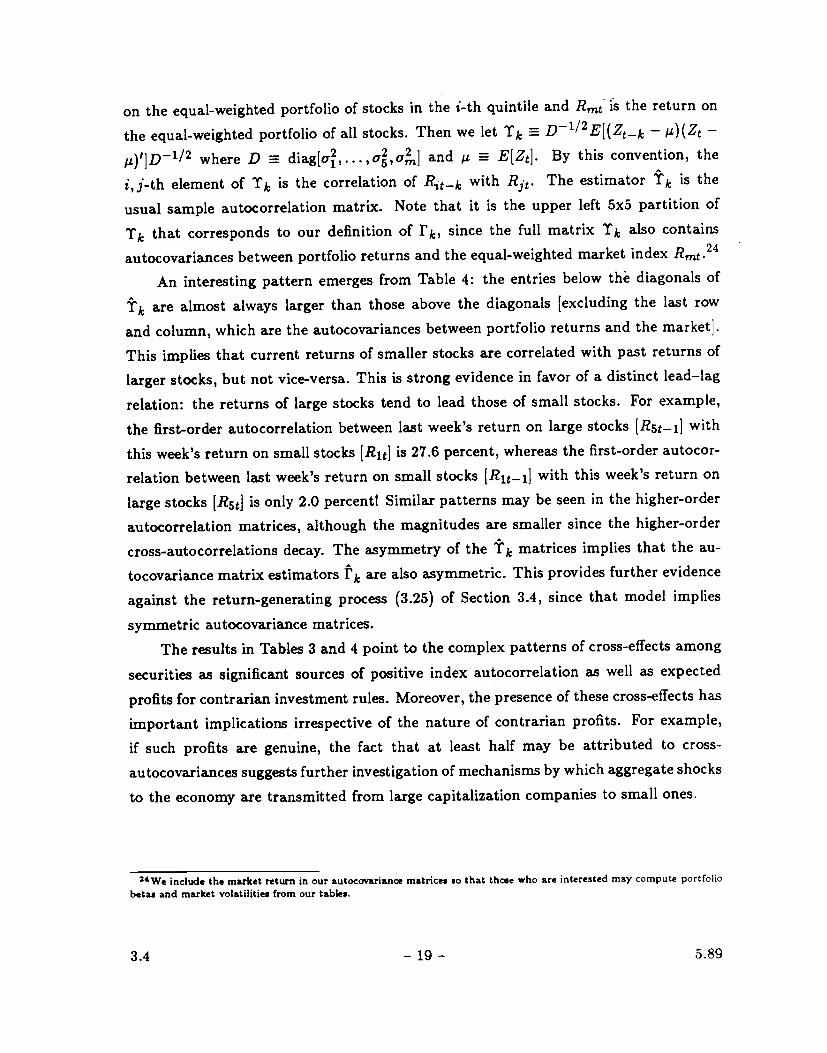
on the equal-weighted portfolio of stocks in the i-th quintile and Rmtis the return on

the equal-weighted portfolio of all stocks. Then we let Tk D_h/2E[(Zt_k — —

j)']D'/2 where D diag[c,. . . and E[Z]. By this convention, the

i,j-th element of Tk is the correlation of R1t_k with R3. The estimator Tk is the

usual sample autocorrelation matrix. Note that it is the upper left 5x5 partition of

Tk that corresponds to our definition of rk, since the full matrix Tk also contains

autocovariances between portfolio returns and the equal-weighted market index Rmt24

An interesting pattern emerges from Table 4: the entries below the diagonals of

are almost always larger than those above the diagonals [excluding the last row

and column, which are the autocovariances between portfolio returns and the marketi.This implies that current returns of smaller stocks are correlated with past returns oflarger stocks, but not vice-versa. This is strong evidence in favor of a distinct lead—lag

relation: the returns of large stocks tend to lead those of small stocks. For example,

the first-order autocorrelation between last week's return on large stocks {R5t_ i] with

this week's return on small stocks [Ru] is 27.6 percent, whereas the first-order autocor-relation between last week's return on small stocks [Rit_i1 with this week's return on

large stocks [R5t] is only 2.0 percent! Similar patterns may be seen in the higher-orderautocorrelation matrices, although the magnitudes are smaller since the higher-ordercross-autocorrelations decay. The asymmetry of the tk matrices implies that the au-

tocovariance matrix estimators rk are also asymmetric. This provides further evidence

against the return-generating process (3.25) of Section 3.4, since that model implies

symmetric autocovariance matrices.

The results in Tables 3 and 4 point to the complex patterns of cross-effects among

securities as significant sources of positive index autocorrelation as well as expected

profits for contrarian investment rules. Moreover, the presence of these cross-effects has

important implications irrespective of the nature of contrarian profits. For example,if such profits are genuine, the fact that at least half may be attributed to cross-autocovariances suggests further investigation of mechanisms by which aggregate shocks

to the economy are transmitted from large capitalization companies to small ones.

34We include the market return in our autocovariance matricee so that thoee who are interested may compute portfoUobetas and market volatilities from our tables.

3.4 — 19 — 5.89

5. Long Horizons Versus Short Horizons.

Since many recent studies have employed longer-horizon returns in examining con-

trarian strategies and predictability of stock returns, we should provide some discussion

of our choice to focus exclusively on weekly returns. Because our analysis of the con-

trarian investment strategy (3.1) uses only short-horizon returns, we have little to say

about the behavior of long-horizon returns. Distinguishing between short and long

return horizons is important, as it is now well-known that weekly fluctuations in stock

returns differ in many ways from movements in three- to five-year returns. There-

fore, inferences concerning the performance of the long-horizon strategies cannot be

drawn directly from short-horizon results such as ours. Nevertheless, some suggestive

comparisons are possible.Statistically, the predictability f short-horizon returns, especially in weekly and

monthly returns, is stronger and more consistent through time. For example, Blumeand Friend (1978) have estimated a time series of cross-sectional correlation coefficients

of returns in adjacent months using monthly New York Stock Exchange data from 1926

to 1975, and found that for 422 of the 598 months the sample correlation was negative.25

This proportion of negative correlations is considerably higher than expected if returnsare unforecastable. Moreover, in their framework a negative correlation coefficient

implies positive expected profits in our equation (3.4) with k = 1. Jegadeesh (1988)

provides further analysis of monthly data and reaches similar conclusions.

The results are even more striking for weekly stock returns. For example, Lo and

MacKinlay (1988) show evidence of strong predictability for portfolio returns usingNew York and American Stock Exchange data from 1962 to 1985. Using the samedata, Lehmann (1988) shows that the profits of a contrarian strategy similar to (3.1)

is virtually always profitable. Not surprisingly, such profits are sensitive to the size

of the transactions costs; for some cases a one-way transactions cost of 0.40 percentis sufficient to render them positive half the time and negative the other half. Theimportance of Lehmann's findings obviously hinge on the relevant costs of turning over

35Sp.cifically, for every pair of adjacent month. t — 1 and t, Blum. and Friend (1978) compute the following statistic p,:

p.E,(Rj,..., — R,.,_1)(R, —

— R,u.*—i)2 /31(R1, —

where R, = . Rfl/N, and N, is the number of securities with non-missing returns in months — 1 and t. Note that pis proportional to the profits (3.3) of the contrarian strategy (3.1) [where the factor of proportionality is always negative[.

3.4 — 20 — 5.89

securities frequently, an issue that is not considered in this paper. However, the factthat our Table 3a shows the smallest firms to be the most profitable on average [asmeasured by the ratio of expected profits to the dollar amount long[ may indicate that

0.80 percent roundtrip transactions costs are low. In addition to the bid-ask spread,which is generally $0.125 or larger and will be a larger percentage of the price forsmaller stocks,26 the price impact of trades on these relatively thinly traded securities

may become important.Evidence regarding the predictability of long horizon returns is somewhat mixed.

Perhaps the most well-known studies of a contrarian strategy using long horizon returns

are those of DeBondt and Thaler (1985, 1987) in which winners are sold and losersare purchased, but where the holding period over which "winning" and "losing" isdetermined is three years. Based on data from 1926 through 1981 they conclude thatthe market overreacts since the losers outperform the winners. However, Chan (1988)

challenges their conclusion and finds that the performance differences can be largely

explained by differences in risk. Moreover, the behavior of DeBondt and Thaler's(1985) cumulative average residual plots, and the results of Lehmann (1989), suggest

that short-horizon return reversals may be responsible for the long-horizon effect.

Fama and French (1988) and Poterba and Summers (1988) have also examinedthe predictability of long horizon returns in a portfolio context, and conclude thatthere is negative serial correlation in long horizon returns — a result which is consistent

with those of DeBondt and Thaler. However, this negative serial dependence is quitesensitive to the sample period employed and may be largely due to the first ten to twenty

years of the 1926 to 1989 samp1e. Furthermore, the statistical procedure on whichthe long-horizon predictability is based has been questioned by Richardson (1988).Richardson has shown that properly adjusting for the fact that multiple time horizons

[and test statisticsl are considered simultaneously yields serial correlation estimates

that are statistically indistinguishable from zero.

These considerations point convincingly to short-horizon returns as the more im-

mediate source from which evidence of predictability and stock market overreaction-

might be culled. Of course, this is not to say that nothing may be gleaned from acareful investigation of returns over longer time spans. Indeed, it may be only at these

26SmaIler itock. tend to have lower price..See Kim, Nel.on, and Start. (1988).

3.4 — 21 — 5.89

lower frequencies that the impact of economic factors such as the business cycle is

detectable. Moreover, to the extent that transaction costs are greater for strategies

exploiting short-horizon predictability, allowing the predictability to persist without

representing any unexploited profit opportunities, long-horizon predictability may be

the more significant issue.

6. Conclusion.

Traditional tests of the random walk hypothesis for stock market prices have gen-

erally focused on either the returns to individual securities or to portfolios of securities.

In this paper we show that the cross-sectional interaction of security returns over time

is an important aspect of stock price dynamics. As anexample, we document the fact

that stock returns are often positively cross-autocorrelated,which reconciles the nega-

tive serial dependence in individual security returns with the positive autocorrelation

in market indexes. This also shows that stock market overreaction need not be the sole

explanation for the profitability in contrarian portfolio strategies. Indeed, the empirical

evidence suggests that less than 50 percent of the expected profits from a contrarian

investment rule may be attributed to overreaction; the majority of such profits is due

to the cross-effects among the securities. We have also shown that these cross-effects

have a very specific pattern for size-sorted portfolios: they display a lead—lag relation,

with the returns of larger stocks generally leading those of smaller ones.The tantalizing question remains: What are the economic sources of positive cross-

autocorrelations across securities? One possibility that is consistent with lead—lag be-

havior is that different sectors of the economy have different sensitivities to macroe-conomic shocks, sensitivities that may be determined by factors such as the degree of

vertical and horizontal integration, concentration, market share, etc. Why this shouldmanifest itself in size-sorted portfolios is still a mystery and remains to be investigated.

3.4 — 22 — 5.89

Appendix 1 — Derivation of (3.4)

N Nirt(k) = = — ,j(Rt_k—R,t_k)R.jt (A1.i)

i=1

N N1— >RitkRit + >Rmt_kRtt (A1.2)--

i=1 i=1

N— 1— -

N -it-kit + R,_kRmt (A1.3)1=1

N1

E[irt(k)} = — — E[R1_E1•] + E[R,_kR] (A1.4)N1=1

N1= —

{cov[1t_k, .ti + +1=1

{COV[R,_k,R1+,} (ALS)

N1 1 2 + (A1.6)— tr(rk) — +

N2--1=1

— ilrk 1N

E[irt(k)] N2— tr(1'j) — — (A1.7)

i=1

3.4 — 23 5.89

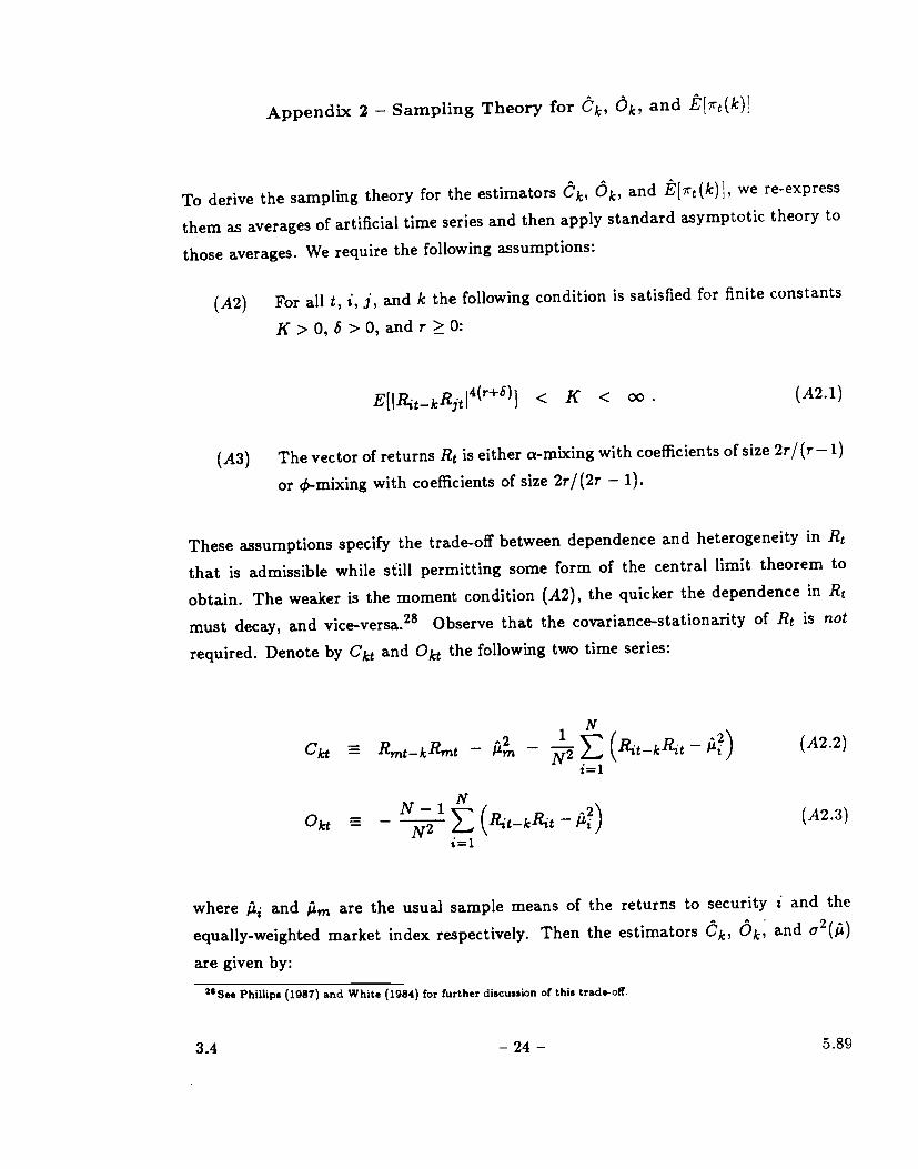
Appendix 2 — Sampling Theory for Ok, 0k' and E{7rt(k)1

To derive the sampling theory for the estimators 0k Ok, and Eirt(kfl, we re-express

them as averages of artificial time series and then apply standard asymptotic theory to

those averages. We require the following assumptions:

(A2) For all t, 1, j, and k the following condition is satisfied for finite constants

K> 0, 5 > 0, and r � 0:

< K < 00 . (A2.1)

(A3) The vector of returns Rt is either a-mixing with coefficientsof size 2r/ (r — 1)

or 4-mixing with coefficients of size 2r/(2r — 1).

These assumptions specify the trade-off between dependence and heterogeneity in R

that is admissible while still permitting some form of the central limit theorem to

obtain. The weaker is the moment condition (A2), the quicker the dependence in R

must decay, and vice-versa.28 Observe that the covariance-stationaritY of R is not

required. Denote by C and O the following two time series:

Ckt Rmt_k1rnt — — — (A2.2)

- N-i (t_kt - (A2.3)

where j2 and j are the usual sample means of the returns to security i and the

equally-weighted market index respectively. Then the estimators Ck, Ok, and 2(i2)are given by:

21 Phillips (1987) and White (1984) for further diecusilon of this trade-off.

3.4 — 24 — 5.89

Ck = T-k Ckt (A2.4)t=k+1

Ok =T—k E °kt (A2.5)

t=k+1

N= — . (A2.6)

Because we have not assumed covariance-stationarity, the population quantities Ckand °k obviously need not be interpretable according to (3.8) since the autocovariance

matrix of R may now be time-dependent. However, we do wish to interpret Ck andas some fixed quantities which are time-independent, thus we require the following:

(A4) The following limits exist and are finite:

1T

lim E[Cj] = Ck (A2.7)t=k+ 1

Turn

1E[OJ (A2.8)T-400T-k t=k+1

Although the expectations E[C1 and E[Okt] may be time-dependent, assumption(A4) asserts that their averages converge to well-defined limits, hence the quantitiesCk and °k may be viewed as "average" cross- and own-autocovariance contributionsto expected profits. Consistent estimators of the asymptotic variance of the estimators

Ck and Ok may then be obtained along the lines of Newey and West (1987), and are

given by ôr and ô respectively, where:

= T-k{

k(O) + 2c5(q)C(j) } (A2.9)

3.4 — 25 — 5.89

=T — k

{Ok(0) + 2a(q)o(i) } (A2.1O)

1 —q±1' q<T

and 'Ck() and ok(j) are the sample j-th order autocovariances of the time series Ckt

and O respectively, i.e.:

=T—k (C_—Ok)(Ckt—Ck) (A2.11)

t=k+j+1

10k(3)=

T — k(O — Ok)(Okt - (A2.12)

t=k+j+1

Assuming that q - o(T1/4), Newey and West (1987) show the consistency of & and

ô under our assumptions (A2)—(A4).29 Observe that these asymptotic variance esti-

mators are robust to general forms of heteroscedasticity and autocorrelation in the Ckt

and O time series. Since the derivation of heteroscedasticity- and autocorrelation-consistent standard errors for the estimated expected profits E[irt(k)] is virtually iden-

tical, we leave this to the reader.

291n our empirical work we choose q = 8.

3.4 — 26 — 5.8

References

Atchison, M., Butler, K. and R. Simouds, 1987, "Nonsynchronous Security Tradingand Market Index Autocorrelation," Journal of Finance 42, 111—118.

Bachelier, L., 1900, Theory of Speculation, reprinted in P. Cootner (ed.), The RandomCharacter of Stock Market Prices, M.I.T. Press, Cambridge, 1964.

Blume, M., and I. Friend, 1978, The Changing Role of the Individual Investor, JohnWiley and Sons, New York.

Chan, K. C., 1988, "On the Return of the Contrarian Investment Strategy," Journalof Business 61, 147—164.

Cohen, K., Maier, S., Schwartz, R. and D. Whitcomb, 1986, The Microstructure ofSecurities Markets, Prentice-Hall, New Jersey.

Conrad, J., Kaul, G. and M. Nimalendran, 1988, "Components of Short-Horizon Secu-rity Returns," working paper, University of Michigan.

Cootner, P., ed., 1964, The Random Character of Stock Market Prices, M.I.T. Press,Cambridge.

DeBondt, W. and R. Thaler, 1985, "Does the Stock Market Overreact?" Journal ofFinance 40, 793—805.

DeBondt, W. and R. Thaler, 1987, "Further Evidence on Investor Overreaction andStock Market Seasonality," Journal of Finance 42, 557—582.

De Long, B., Shleifer, A., Summers, L. and R. Waldmann, 1989, "Positive FeedbackInvestment Strategies and Destabilizing Rational Speculation," NBER Working Pa-per No. 2880.

Fama, E., 1970, "Efficient Capital Markets: A Review of Theory and Empirical Work,"Journal of Finance 25, 383—417.

Fama, E. and K. French, 1988, "Permanent and Temporary Components of StockPrices," Journal of Political Economy 96, 246—273.

Jegadeesh, N., 1988, "Evidence of Predictable Behavior of Security Returns," AndersonGraduate School of Management Working Paper #6—88, U.C.L.A.

Kim, M., Nelson, C. and R. Startz, 1988, "Mean Reversion in Stock Prices? A Reap-praisal of the Empirical Evidence," NBER Working Paper No. 2795.

Lehmann, B., 1988, "Fads, Martingales, and Market Efficiency," NBER Working PaperNo. 2533, to appear in Quarterly Journal of Economics.

Lehmann, B., 1989, "Winners, Losers, and Mean Reversion in Weekly Equity Returns,"unpublished working paper.

3.4 — 27 — 5.89

Leroy, S. F., 1973, "Risk Aversion and the Martingale Property of Stock Returns"International Economic Review 14, 436—446.

Lo, A. W. and A. C. MacKinlay, 1988, "Stock Market Prices Do Not Follow RandomWalks: Evidence From a Simple Specification Test," Review of Financial Studies 1.

41—66.

Lo, A. W. and A. C. MacKinlay, 1989, "An Econometric Analysis of Nonsynchronous-Trading," Sloan School of Management Working Paper No. 3003—89—EFA, Mas-sachusetts Institute of Technology.

Lucas, R. E., 1978, "Asset Prices in an Exchange Economy," Econometrica 46, 1429—

1446.

Newey, W. K. and K. D. West, 1987, "A Simple Positive Definite, Heteroscedasticityand Autocorrelation Consistent Covariance Matrix," Econometrica 55, 703—705.

Phillips, P.C.B, 1987, "Time Series Regression with a Unit Root," EconOrnetrica 55,277—302.

Poterba, J. and L. Summers, 1988, "Mean Reversion in Stock Returns: Evidence andImplications," Journal of Financial Economic8 22, 27—60.

Richardson, M., 1988, "Temporary Components of Stock Prices: A Skeptic's View,"unpublished working paper.

Roll, R., 1984, "A Simple Implicit Measure of the Effective Bid-Ask Spread in anEfficient Market," Journal of Finance 39, 1127—1140.

Scholes, M. and J. Williams, 1977, "Estimating Beta From Non-Synchronous Data,"Journal of Financial Economics 5, 309—327.

Shefrin, H. and M. Statman, 1985, "The Disposition to Ride Winners Too Long andSell Losers Too Soon: Theory and Evidence," Journal of Finance 41, 774—790.

Summers, L., 1986, "Does the Stock Market Rationally Reflect Fundamental Values?,"Journal of Finance 41, 591—600.

White, H., 1984, Asymptotic Theory for Econometricians, Academic Press, New York.

3.4.

—28-- 5.89

</ref_section>

Aut

ocor

rela

tion

coef

fici

ents

for

the

wee

kly

equa

l-w

eigh

ted

(Pan

el A

) an

d va

lue-

wei

ghte

d (P

anel

B)

CR

SP N

YSE

—A

ME

X

stoc

k

retu

rns

inde

xes,

for

the

sam

ple

peri

od 6

Jul

y 19

62 to

31

Dec

embe

r 198

7 an

d su

b-pe

riod

s. M

eans

and

sta

ndar

d de

viat

ions

are

also

repo

rted

(in

per

cent

ages

), an

d he

tero

sced

astic

ity-c

onsi

sten

t sta

ndar

d er

rors

for

auto

corr

elat

ion

coef

fici

ents

are

giv

en i

n pa

rent

hese

s.

Tim

e Pe

riod

Sa

mpl

e Si

ze

Mea

n x

100

Std.

Dev

. x

100

(SE

) h (SE

)

P3

(SE

) P

4

(SE

)

Pane

l A:

6207

06 —

871

231

6207

06 —

75

0403

7504

04 —

87

1231

1330

665

665

0.35

9

0.26

4

0.45

5

2.27

7

2.32

6

2.22

5

0.29

6 (0

.046

)

0.33

8

(0.0

53)

0.24

8

(0.0

76)

0.11

6

(0.0

37)

0.15

7

(0.0

48)

0.07

1

(0.0

58)

0.08

1

(0.0

34)

0.08

2

(0.0

52)

0.07

8

(0.0

42)

0.04

5

(0.0

35)

0.04

4

(0.0

53)

0.04

0 (0

.045

)

Pane

l B:

6207

06 —

871

231

1330

0.

210

2.05

8 0.

074

0.00

7 0.

021

—0.

005

(0.0

40)

(0.0

37)

(0.0

36)

(0.0

37)

6207

06 —

75

0403

66

5 0.

135

1.97

2 0.

055

0.02

0 0.

058

-0.0

21

(0.0

58)

(0.0

55)

(0.0

60)

(0.0

58)

7504

04

8712

31

665

0.28

5 2.

139

0.09

1 -0

.003

—

0.01

4 0.

007

(0.0

55)

(0.0

49)

(0.0

42)

(0.0

46)

3.2

11.8

8

Tab

le lb

Aut

ocor

rela

tion

coef

ficie

nts f

or th

e da

ily e

qual

-wei

ghte

d (P

anel

A) a

nd va

lue-

wei

ghte

d (P

anel

B)

CR

SP N

YSE

—A

ME

X s

tock

ret

urns

inde

xes,

for

the

sam

ple p

erio

d 3

July

196

2 to

31

Dec

embe

r 19

87 a

nd s

ub-p

erio

ds.

Mea

ns a

nd s

tand

ard

devi

atio

ns a

re a

lso

repo

rted

(in

perc

enta

ges)

, and

het

eros

ceda

stic

ity-c

onsi

sten

t stan

dard

err

ors f

or a

utoc

orre

latio

n co

effi

cien

ts a

re g

iven

in

pare

nthe

ses.

Tim

e Pe

riod

Sa

mpl

e M

ean

Std.

Dev

. P3

P

4

Siz

e x

100

x 10

0 (S

E)

(SE

) (S

E)

(SE

)

Pane

l A:

6207

03 —

871

231

6408

0.

073

0.81

1 0.

355

0.08

8 0.

088

0.10

4

(0.0

38)

(0.0

4 1)

(0.0

33)

(0.0

27)

6207

03 —

750

428

3204

0.

054

0.80

3 0.

425

0.12

7 0.

144

0.13

7

(0.0

33)

(0.0

32)

(0.0

29)

(0.0

29)

7504

29 —

871

231

3204

0.

091

0.81

8 0.

287

0.05

0 0.

034

0.07

3

(0.0

67)

(0.0

73)

(0.0

59)

(0.0

44)

Pane

l B:

6207

03 —

87

1231

64

08

0.04

3 0.

842

0.20

0 —

0.00

9 0.

006

—0.

001

(0.0

28)

(0.0

40)

(0.0

31)

(0.0

19)

6207

03 —

75

0428

32

04

0.02

9 0.

753

0.28

2 0.

016

0.04

1 0.

028

(0.0

28)

(0.0

29)

(0.0

27)

(0.0

27)

7504

29—

8712

31

3204

0.

057

0.92

2 0.

146

—0.

026

-0.0

17

0.02

1

(0.0

42)

(0.0

64)

(0.0

49)

(0.0

26)

Aut

ocor

rela

tion

coef

fici

ents

for

the

mon

thly

equ

al-w

eigh

ted

(Pan

el A

) an

d va

lue-

wei

ghte

d (P

anel

B)

CR

SP N

YSE

—A

ME

X

stoc

k

retu

rns

inde

xes,

for

the

sam

ple p

erio

d 31

Aug

ust 1

962

to 31

Dec

embe

r 19

87 a

nd su

b-pe

riod

s. M

eans

and

stan

dard

dev

iatio

ns a

re a

lso

repo

rted

(in

per

cent

ages

), an

d he

tero

sced

astic

ity-c

onsi

sten

t sta

ndar

d er

rors

for a

utoc

orre

latio

n co

effi

cien

ts a

re g

iven

in

pare

nthe

ses.

Tim

e Pe

riod

Sa

mpl

e Si

ze

Mea

n x

100

Std.

Dev

. x

100

(SE

) h (SE

) P

3

(SE

) P

4

(SE

)

Pane

l A:

6208

31 —

871

231

6208

31 —

75

0430

7505

30 —

87

1231

305

153

152

1.29

3

0.88

9

1.70

0

6.19

3

6.56

0

5.79

4

0.14

8

(0.0

60)

0.14

5

(0.0

84)

0.14

1

(0.0

79)

—0.

034

(0.0

61)

—0.

009

(0.0

93)

—0.

087

(0.0

69)

—0.

011

(0.0

54)

0.05

4

(0.0

80)

—0.

121

(0.0

66)

0.00

3

(0.0

60)

0.00

4

(0.0

89)

—0.

046

(0.0

64)

Pane

l B:

6208

31 —

871

231

305

0.96

4 4.

552

0.04

2 —

0.05

1 0.

020

0.01

4

(0.0

65)

(0.0

63)

(0.0

65)

(0.0

58)

6208

31 —

750

430

153

0.67

8 4.

363

0.05

5 —

0.02

4 0.

099

0.06

3

(0.1

03)

(0.0

97)

(0.1

16)

(0.0

91)

7505

30 —

87

1231

15

2 1.

252

4.73

2 0.

019

—0.

089

-0.0

60

—0.

058

(0.0

82)

(0.1

78)

(0.0

68)

(0.0

70)

3.2

11.8

8

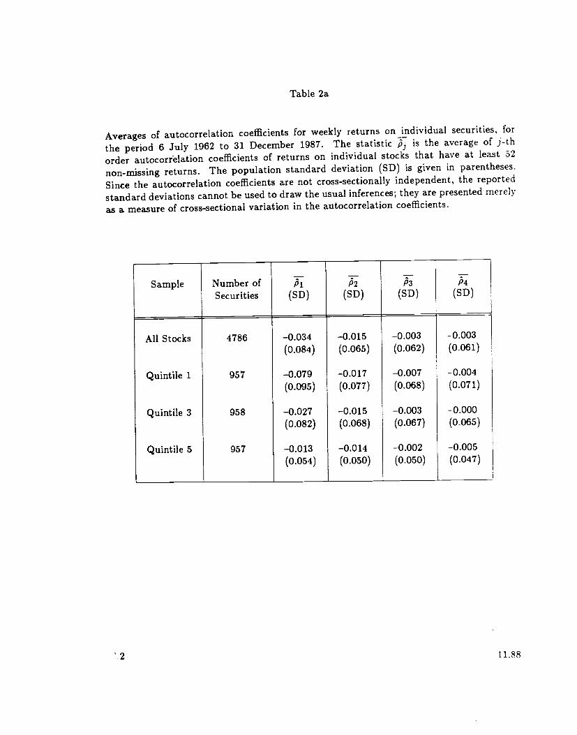
Table 2a

Averages of autocorrelation coefficients for weekly returns on individual securities, forthe period 6 July 1962 to 31 December 1987. The statistic is the average of j-thorder autocorrèlatiofl coefficients of returns on individual stocks that have at least 52non-missing returns. The population standard deviation (SD) is given in parentheses.Since the autocorrelation coefficients are not cross-sectionally independent, the reportedstandard deviations cannot be used to draw the usual inferences; they arepresented merelyas a measure of cross-sectional variation in the autocorrelation coefficients.

Sample Number ofSecurities (SD)

12

(SD)/3,3

(SD)34

(SD)

All Stocks

Quintile 1

Quintile 3

Quintile 5

4786

957

958

957

—0.034

(0.084)

—0.079

(0.095)

—0.027

(0.082)

—0.013

(0.054)

—0.015

(0.065)

—0.017

(0.077)

—0.015

(0.068)

—0.014

(0.050)

—0.003

(0.062)

—0.007

(0.068)

—0.003

(0.067)

—0.002

(0.050)

—0.003

(0.061)

—0.004

(0.071)

—0.000

(0.065)

—0.005

(0.047)

'.2 11.88

Table 2b

Averages of autocorrelation coefficients for daily returns on individual securities, for theperiod 3 July 1962 to 31 December 1987. The statistic is the average of j-th orderautocorrelation coefficients of returns on individual stocks that have at least 52 non-missingweekly returns. The population standard deviation (SD) is given in parentheses. Since theautocorrelation coefficients are not cross-sectionally independent, the reported standarddeviations cannot be used to draw the usual inferences; they are presented merely as ameasure of cross-sectional variation in the autocorrelation coefficients.

Sample Number ofSecurities

h(SD)

,(SD) (SD)

,5(SD)

All Stocks

Quintile 1

Quintile 3

Quintile 5

4786

957

958

957

—0.014

(0.101)

—0.093

(0.106)

—0.008

(0.094)

0.048(0.065)

—0.016

(0.041)

—0.020

(0.043)

—0.015

(0.042)

—0.015

(0.033)

—0.015

(0.036)

—0.017

(0.040)

—0.017

(0.038)

—0.017

(0.029)

—0.006

(0.034)

—0.008

(0.041)

—0.005

(0.035)

—0.008

(0.028)

3.2 11.88

Table 2c

Averages of autocorrelatiOn coefficients for monthly returns on individual securities, forthe period 31 August 1962 to 31 December 1987. The statistic is the average of j-thorder autocorrelation coefficients of returns on individual stocks that have at least 24 non-

missing monthly returns. The population standard deviation (SD) is given in parentheses.Since the autocorrelation coefficients are not cross-sectionally independent, the reportedstandard deviations cannot be used to draw the usual inferences; they are presented merelyas a measure of cross-sectional variation in the autocorrelation coefficients.

Sample Number ofSecurities

-(SD)

-,5

(SD)

-P3

(SD)

-P4

(SD)

All Stocks

Quintile 1

Quintile 3

Quintile 5

4472

894

894

894

—0.029

(0.111)

—0.055

(0.131)

—0.019

(0.112)

—0.016

(0.084)

—0.017

(0.100)

—0.011

(0.115)

—0.011

(0.101)

—0.028

(0.079)

—0.002

(0.098)

—0.007

(0.113)

0.003

(0.097)

—0.005

(0.079)

—0.001

(0.094)

0.005

(0.107)

0.002(0.087)

—0.004

(0.077)

3.2 11.88

Table 3a

Analysis of the profitability of the return-reversal strategy applied to weekly returns, for the sample of 551 CRSP NYSE—AMEX stocke with non-missing weekly returns from 6 July 1962 to 31 December 1987 (1330 weeks). Expected profits is gwenby E(re(k)] = C, + O — c2(M), where Ckdepends only on cross-autocovariances and O, depends only on own-autocovariances.All s-stat,stics are asymptotically N(0,1) under the null hypothesis that the relevant population value is zero, and are robust toheteroscedasticity and autocorrelation. The average long position I(k) is also reported, with its sample standard deviation inparentheses underneath. The analysis is conducted for all stocks as well as for the five size-sorted quintiles; to conserve space,results for the second and fourth quintilea have been omitted.

Portfolio Lagk

O'(!-stat)

O'(a-stat)

c2(j1)' EfT.(k))'(a-stat)

I(k)'(SD')

%-Ok %-O %2()

All Stocks

Quintile 1

Quintile 3

Quintile 5

1

1

1

1

0.841(4.95)2.048(6.36)0.703(4.67)0.188(1.18)

0.862(4.54)2.493(7.12)0.366(2.03)0.433(2.61)

0.009

0.009

0.011

0.005

1.694(20.81)4.532

(18.81)1.058

(13.84)0.617

(11.22)

151.9(31.0)208.8(47.3)138.4(32.2)117.0(28.1)

49.6

45.2

66.5

30.5

50.9

55.0

34.6

70.3

—0.5

—0.2

—1.0

—0.8

All Stocks

Quintile 1

Quintile 3

Quintile 5

2

2

2

2

0.253(1.64)0.803(3.29)0.184(1.20)

—0.053

(—0.39)

0.298(1.67)0.421(1.49)0.308(1.64)0.366(2.28)

0.009

0.009

0.011

0.005

0.542(10.63)1.216(8.86)0.481(7.70)0.308(5.89)

151.8(31.0)208.8(47.3)138.3(32.2)116.9(28.1)

46.7

66.1

38.3

—17.3

54.9

34.7

64.0

118.9

—1.6

—0.7

—2.3

—1.6

All Stocks

Quintile 1

Quintile 3

Quintile &

3

3

3

3

0.223(1.60)0.552(2.73)0.237(1.66)0.064(0.39)

—0.066

(—0.39)0.038(0.14)

—0.192

(—1.07)—0.003

(—0.02)

0.009

0.009

0.011

0.005

0.149(3.01)0.582(3.96)0.035(0.50)0.056(1.23)

151.7(30.9)208.7(47.3)138.2(32.1)116.9(28.1)

149.9

94.9

677.6

114.0

—44.0

6.6

—546.7

—5.3

—5.9

—1.5

—30.9

—8.8

All Stocks

Quintile 1

Quintile 3

Quintile 5

4

4

4

4

0.056(0.43)0.305(1.53)0.023(0.18)—0097(—0.65)

0.083(0.51)0.159(0.59)—0.045

(—0.26)0.128(0.77)

0,009

0.009

0.011

0.005

0.130(2.40)0.455(3.27)

—0.033

(—0.44)0.026(0.52)

151.7(30.9)208.7(47.3)138.2(32.0)116.8(28.0)

43.3

67.0

—374.6

63.5

34.9

.&

403.4

—6.7

—1.9

.b

—18.8

'Multiplied by 10000.Not computed when expected profits are negative.

3.3 11 88

Table 3b

Analysis of the profitability of the return-reversal strategyapplied to weekly returns, for the sample of 949 CRSP NYSE—A.MEX

stocks with non-missing weekly returns during the period 6 July 1962 to 3 April 1975 (665 weeks). Expected profits is given

by E[irg (k)1 = Ct + Ok — a(M), where Ct depends only on crossautocovariaflC and O depends only on own.autocovariances

All s-statisticS are asymptotically N(O1) under the null hypothesisthat the relevant population value is zero, and are robust to

heteroscedasticity and autocorrelation. The average long position I(k) is also reported, with its sample standard deviation ri

parentheses underneath. The analysis is conducted for all stocks as well as for the five size-sorted quintiles to conserve space,

results for the second and fourth quintiles have been omitted.

Multiplied by 10,CX)O.' Not computed when expected profits are negative.

11883.3

[ortfolio Lag(s—st at)

Ok(s_stat) (s_stat)

,(k) %-Ot(SD5)

%-Ot

All Stocks 1

Quintile 1 1

Quintile 3 1

Quintile 5 1

1.194(5.34)2.409(6.73)1.196(5.10)0.302(1.53)

1.191(4.61)3.533(8.84)u.445(1.50)0.380(1.64)

0.019

0.020

0.020

0.015

2.366(15.36)5.923

(16.63)1.621

(10.85)0.668(9.82)

164.0(35.3)221.8(49.0)154.4(35.4)119.8(28.5)

50.5

40.7

73.8

45.2

50.3

59.7

27.5

57.0

—0.8

—0.3

—1.3

—2.2

All Stocks

Quintile 1

Quintile 3

Quintile 5

2

2

2

2

0.566(2.80)1.128(3.83)0.539(2.59)0.149(1.09)

0.192(0.86)0.305(0.86)0.164(0.73)0.248(1.47)

0.019

0.020

0.020

0.015

0.739(9.16)1.413

(7.71)0.682(6.46)0.382(5.52)

164.0(35.3)221.8(49.1)154.3(35.4)119.8(28.6)

76.6

79.8

78.9

38.9

26.0

21.6

24.0

65.0

—2.6

—1.4

—3.0

—3.9

All Stocks

Quintile 1

Quintile 3

Quintile 5

3

3

3

3

0.314(1.42)0.583(2.06)0.385(1.61)0.227(1.05)

—0.062

(—0.24)0.156(0.45)

—0.174

(—0.61)—0.044

(—0.17)

0.019

0.020

0.020

0.015

0.232(3.02)0.719(4.06)0.190(1.83)0.168(2.73)

163.9(35.3)221.7(49.1)154.2(35.4)119.7(28.6)

135.2

81.1

202.1

134.7

—26.9

21.7

—91.4

—26.0

—8.3

—2.7

—10.7

-8.8

All Stocks

Quintile 1

Quintile 3

Quintile 5

4

4

4

4

0.149(0.78)0.347(1.17)0.169(0.84)-0.025(—0.14)

0.030(0.13)0.103(0.27)—0.152

(—0.62)0.075(0.38)

0.019

0.020

0.020

0.015

0.159(2.18)0.430(2.64)—0.)4(—0.04)0.035(0.69)

163.8 93.2(35.2)221.6 80.8

(49.1)154.0(35.1)119.6 —71.4

(28.6)

19.0 —12.1

23.8 —4.6

b

213.2 —41.8

Table 3c

Analysis of the profitability of the return-reversal strategy applied to weekly returns, for the sample of 1172 CRSP NYSE—AMEX stocks with non-milling weekly returns during the period 4 April 1975 to 31 December 1987 (665 weeks). Expectedprofits is given by EIs's(k)] = Ck + Ok o-2(M), where C depends only on cross-autocovariances and O& depends only onown-autocovariance,. All v-statistics are asymptotically N(0,1) under the null hypothesis that the relevant population valueis vero, and are robust to heteroscedasticity and autocorrelation. The average long position 16(k) is also reported, with itssample standard deviation in parentheses underneath. The analysis is conducted for all stocks as well as for the five live-sortedquintiles; to conserve space, results for the second and fourth quintiles have been omitted.

Portfolio Lagk

Oj'(r.stat)

ô'(v-stat)

c2()' Ets(k)]'(a-stat)

[t(k)'(SD')

%-Ok %-O %-o(j)

All Stocks

Quintile 1

Quintile 3

Quintile 5

1

1

1

1

1.022

(3.16)1.897(3.83)1.038(3.10)0.465(1.77)

1.105(3.10)2.873(5.18)0.689(1.88)0.368(1.47)

0.026

0.031

0.031

0.014

2.101(17.05)4.739

(15.25)1.696

(12.43)0.819(9.58)

167.7(31.5)217.8(47.2)161.4(31.7)128.9(28.8)

48.7

40.0

61.2

56.7

52.6

60.6

40.6

44.9

—1.2

—0.6

—1 8

—1.7

All Stocks

Quintile 1

Quintile 3

Quintile 5

2

2

2

2

0.211(0.75)0.788(1.92)0.220(0.79)—0.083

(-0.33)

0.438(1.36)0.665(1.57)0.237(0.68)0.317(L09)

0.026

0.031

0.031

0.014

0.622(8.38)1.422(7.72)0.426(3.65)0.220(3.04)

167.5(31.4)217.7(47.2)161.2(31.5)128.9(28.8)

33.8

55.4

51.7

—37.8

70.4

46.7

55.6

144.0

—4.2

—2.2

—7.4

-6.2

All Stocks

Quintile 1

Quintile 3

Quintile 5

3

3

3

3

0.277(1.30)0.816(3.05)0.277(1.19)—0.028

(—0.13)

—0.025

(—0.10)—0.178

(—0.54)0.109(0.39)0.042(0.18)

0.026

0.031

0.031

0.014

0.225(3.22)0.608(3.69)0.354(3.83)0.000(0.01)

167.4(31.2)217.5(47.1)161.0(31.2)128.8(28.7)

122.9

134.3

78.2

—7949.7

—11.3

—29.3

30.7

11873.6

—11.6

—5 1

-8.8

—3823.9

All Stocks

Quintile 1

Quintile 3

Quintile 5

4

4

4

4

0.098(0.45)0.407(1.50)0.124(0.55)-'0.034(—0.15)

0.088(0.34)0.063(0.19)

—0.054

(—0.20)0.104(0.42)

0.026

0.031

0.031

0.014

0.160(2.09)0.439(2.57)0.038(0.38)0.056(0.84)

167.3(31.1)217.5(47.2)160.9(31.0)128.7(28.7)

61.2

92.8

324.3

—61.1

55.2

14.2

—142.2

185.3

—16.4

—7.0

—82.0

—24.1

Multiplied by 10,000.

3.3 11.88

11.883.3

Table 4

Autocorrelatiofl matrices of the vector Z [R1 R2 R3 R4 R5 Rmt]' where .R, is the return on the

portfolio of stocks in the i-th quintile, i = 1,. . . , 5 and Rmt is the return on the equal-weighted index, for

the sample of 551 stocks with non-missing weekly returns from 6 July 1962 to 31 December 1987 (1330

observations). Note T D"2E1(Zt_k — ,A)(Zt — )']D"2, where D diagcr,. .. ,o, Asymptotic

standard errors for the autocorrelatiOns under an i.i.d. null hypothesis are given by — = 0.027.

0.919 0.857 0.830 0.747 0.918R 1.0001.000 0.943 0.929 0865 0.976

R2 0.9190.857 0.943 1.000 0.964 0.925 0.979

T0 = R3R4R5Rrr,

0.8300.7470.9 18

0.9290.8650.976

0.9640.9250.979

1.0000.9460.974

0.9461.0000.933

0.9740,9331.000

R1112

R10.3330.334

112

0.2440.2520.265

R30.1430.1570.175

R40.1010.1220.140

R50.0200.0330.051

Rm0.1840.1950.207

T1 — RR4RRm

0.3250.3160.2760.333

0.2620.2300.262

0.1770.1540.168

0.1390.1220.130

0.0500.0440.041

0.2040.1780.202

.R1112

R0.1300.133

112

0.0870.1010.088

R30.0440.0580.046

114

0.0220.0390.027

R50.0050.0170.002

R,,0.0640.0760.061

—2 — 113

R4RRm

0.1140.1010.0670.115

0.0850.0550.087

0.0480.0200.045

0.029 0.0080.008 —0.012

0.026 0.004

0.0590.0310.061

R1112

R0.0890.094

R20.0470.0660.079

R30.0150.0380.059

R40.0130.0410.061

R—0.005

0.0180.041

Rm0.0360.0560.072

—— 1?R4RRm

0.0840.0530.087

0.0670.0440.063

0.0470.0310.038

0.0490.0340.040

0.0310.0150.020

0.0590.0380.054

R112

R10.0500.0640.065

112

0.0010.0230.029

113

—0.014—0.002

0.006

R4—0.029—0.012—0.002

R5—0.030—0.020—0.017

Rvn

—0.0020.0140.019

113

114

R50.0720.048

0.0420.023

0.0170.0020.001

0.005—0.007

0.010

—0.008—0.022—0.021

0.0290.0110.014