NBER WORKING PAPER SERIES

WELFARE TRANSITIONS IN THE 1990s: THE ECONOMY, WELFARE POLICY, AND THE EITC

Jeffrey Grogger

Working Paper 9472http://www.nber.org/papers/w9472

NATIONAL BUREAU OF ECONOMIC RESEARCH1050 Massachusetts Avenue

Cambridge, MA 02138January 2003

The author gratefully acknowledges support from the Administration for Children and Families, U.S.Department of Health and Human Services. However, opinions and conclusions expressed herein are thoseof the author, and do not necessarily represent the positions of ACF, HHS, or any other government agency.I thank Duncan MacRae for extraordinary research assistance and seminar participants at Texas A&M andthe University of Texas for helpful comments. The views expressed herein are those of the authors and notnecessarily those of the National Bureau of Economic Research.

©2003 by Jeffrey Grogger. All rights reserved. Short sections of text not to exceed two paragraphs, may bequoted without explicit permission provided that full credit including notice, is given to the source.

Welfare Transitions in the 1990s: The Economy, Welfare Policy, and the EITC Jeffrey GroggerNBER Working Paper No. 9472January 2003JEL No. I3

ABSTRACT

The rapid decline in the welfare caseload remains a subject of keen interest to both policymakers

and researchers. In this paper, I use data from the Survey of Income and Program Participation

spanning the period from 1986 to 1999 to analyze how the economy, welfare reform, the Earned

Income Tax Credit, and other factors influenced welfare entries and exits, which in turn affect the

caseload. I find that the decline in the welfare caseload resulted from both increases in exits and

decreases in entries. Entries were most significantly affected by the economy, the decline in the real

value of welfare benefits, and the expansion of the EITC. The EITC had substantial effects on initial

entries onto welfare. Exits were most significantly affected by the economy and federal welfare

reform. Federal reform had its greatest effects on longer-term spells of the type generally

experienced by more disadvantaged recipients. Some out-of-sample predictions help explain the

otherwise puzzling observation that, despite substantial increases in the unemployment rate since

2000, caseloads have remained roughly constant.

Jeffrey Grogger School of Public Policy UCLA 405 Hilgard Avenue Los Angeles, CA 90095-1656 and NBERjgrogger@ucla.edu

I. Introduction

The 1990s were a volatile time for the U.S. welfare system. At the beginning of the

decade, 4.1 million families received payments under the Aid to Families with Dependent

Children (AFDC) program. By 1994, that number had risen to 5 million. The caseload then

plummeted to 2.6 million families in 1999. Those families represented only 2.6 percent of the

U.S. population, the smallest proportion receiving aid since 1967 (U.S. Department of Health

and Human Services 2002).

A substantial body of research has attempted to explain these changes. Most studies have

focused on two factors: the economy and welfare reform. The welfare caseload began to rise as

the economy entered a recession during 1990-91. It fell as the economy expanded. At the same

time, many states began reforming their welfare programs under waivers from the AFDC

program. In 1996, Congress passed the Personal Responsibility and Work Opportunity

Reconciliation Act (PRWORA). As a result, all states replaced AFDC with Temporary

Assistance for Needy Families (TANF) between 1996 and 1998. Compared to AFDC, in most

states TANF imposes greater work requirements, greater sanctions for violating those

requirements, and limits on the amount of time that recipients can receive aid.

Most studies agree that both welfare reform and the economy played important roles in

reducing the caseload between 1994 and 1999.1 A few studies point to other factors as well.

MaCurdy, Mancuso, and O'Brien-Strain (2002) show that the decline in the real value of welfare

benefits also contributed to the decline in caseloads. Grogger (2003, forthcoming) reports that

1 See Blank 2000; CEA 1997, 1999; Grogger 2000; Huang, et al. 2000; Levine and Whitmore 1998; O'Neill and Hill 2001; Schoeni and Blank 2000; Wallace and Blank 1999. Three studies are outliers. Ziliak, et al. (2000) and Figlio and Ziliak (1999) estimate that welfare reform actually increased the caseload, albeit insignificantly. Rector and Youseff (1999) estimate that the economy had no effect on caseloads. See Blank (2002) and Grogger, Karoly, and Klerman (2002) for detailed reviews.

2

the Earned Income Tax Credit (EITC) played a particularly strong role in reducing the welfare

participation rate.

In this study I estimate the effects of the economy and policy changes on welfare flows,

that is, entries and exits, rather than the stock measures of welfare receipt that have been the

focus of most previous analyses. At first glance, one might expect stocks and flows to provide

essentially equivalent information, since they are linked by a simple transition rule. Yet there are

reasons to think that flows might be more informative and of substantial interest in their own

right.

First, entry effects may weigh in at least some observers evaluation of the success of

welfare reform. Conservative proponents of reform explicitly sought to reduce welfare entries,

particularly entries related to unwed childbearing (see R. Kent Weaver, 2000, ch. 6 ). Such

observers might question the success of welfare reform if the decline in the caseload resulted

entirely from increased exits.

Entry effects may also have implications for the provision of in-kind transfers.

Historically, both Food Stamps and Medicaid were closely linked to welfare: families typically

applied for welfare and Food Stamps at the same time, and Medicaid insurance for families was

limited to families on welfare. If families primarily learn about non-cash transfer programs

when they first apply for welfare, then policy interventions that reduce welfare entry could also

reduce take-up of such safety net services.

Furthermore, entry effects may affect one's interpretation of recent research on welfare

reform. Since welfare reform experiments are based on welfare participants, they reveal

primarily how policy reforms affect welfare exits.2 So-called "leaver" studies, which track

families as they move off the welfare rolls, explicitly focus on the behavior of families exiting 2 See Grogger, Karoly, and Klerman (2002) for a comprehensive review of numerous reform experiments.

3

welfare. However, if recent policy changes have had important effects on welfare entries, then

such studies provide only a partial portrayal of how those changes have affected life in the low

end of the income distribution.

Finally, accounting for the link between stocks and flows reveals inertia in welfare

caseloads. Even though economic and policy changes may affect entries and exits

contemporaneously, it takes time for those changes to fully manifest themselves in the welfare

caseload. As a general proposition, this point has been recognized by others (Klerman and

Haider 2002). Here I show that it helps to explain the otherwise puzzling observation that,

despite large increases in unemployment between 2000 and 2002, the caseload has remained

roughly constant.

Welfare entries and exits have been the focus of a handful of prior welfare reform studies.

However, those studies have been based on relatively small samples. This has sometimes

resulted in precision problems, which have been further exacerbated by the fact that welfare

transitions are relatively rare events. In addition, most previous studies have involved sample

periods that include only one or two years of post-reform data, which also has made it difficult to

estimate the effects of reform with much precision.

As a result, previous estimates are quite mixed, and in many cases, they run contrary to

expectations. For example, Ribar's (2002) analysis of SIPP data from 1991 to 1995 yields a

marginally significant estimate suggesting that waiver-based reforms actually decrease welfare

exit (which would increase welfare use) while having no effect on entry. Acs et al. (2002) use

SIPP data covering the periods 1990-1992 and 1996-1998 to study the effects of several types of

welfare reform policies. They find that several types of waiver-based reforms increase exit, but

generally find no effect on entry. Gittleman (2001) studies a sample from the Panel Study of

4

Income Dynamics (PSID) that extends through 1995. He finds that waivers increase exits, but

also finds that they increase entries. Hofferth et al. (2000a, b), also analyzing the PSID, estimate

the effects of several reforms, as did Acs, et al. (2002). They find work requirements and

sanctions to increase exits, although six of the seven reforms they consider have insignificant

effects on entry. Finally, using administrative data from five urban counties, Mueser et al.

(2000) report that reform decreases entry and increases exit. Although their findings are mostly

consistent with expectations, there are questions about the extent to which their results are

representative of the nation as a whole.

My analysis employs SIPP data spanning the period from 1986 through 1999. These data

alleviate some of the problems confronting earlier researchers. My sample sizes are substantially

larger than those of earlier analyses, which helps solve the precision problem, and generally

results in estimates that are consistent with expectations. The longer sample period has the

advantage of allowing me to estimate the effect of TANF, rather than being restricted to the

effect of waiver-based reform. A final advantage of my analysis is its inclusion of the EITC,

which proves to be empirically important.

In the next section of the paper, I discuss the data. Section III discusses the analytical

methods. In section IV I present regression results. In section V I use those results to

decompose the decline in welfare participation rates into components attributable to changes in

the economy, changes in policy, and other factors. In Section VI I use the estimation results to

make predict how recent changes in the economy should affect welfare participation rates.

Section VII concludes.

5

II. The Data

A. Background on the SIPP

The SIPP consists of a number of panels, each of which is a longitudinal probability

sample of the U.S. population. In this study I include data from the 1986, 1987, 1988, 1990,

1991, 1992, 1993, and 1996 panels.3 The duration of the panels varies between 24 months (the

1988 panel) and 48 months (the 1996 panel). Thus the sample period extends from 1986 through

1999.

The panels are divided into waves, or four-month intervals at which the core module

questionnaire is administered. The core module provides extensive information about the

behavior of panel respondents, including their welfare use. At each wave, the SIPP asks

respondents about their welfare use in each of the previous four months. Although these data

could be used to construct monthly welfare-use records, they suffer from "seam bias," meaning

that reported transitions are much more likely to occur between waves rather than within waves.4

For this reason, I only make use of data from month 4 of each wave.

An entry occurs in wave t if the respondent was not receiving aid at wave t-1 but received

aid in month t. An exit occurs if she received welfare in wave t-1 but not in wave t.

Participation rates at wave t are calculated as the number of persons on aid at wave t divided by

the number of persons in the sample.

The sample is restricted to low-skill women, defined as women with a high-school

diploma or less, who are between the ages of 15 and 54. These women constitute the vast

majority of all adult welfare recipients. SIPP respondents are classified on the basis of their age

3 The 1989 panel was truncated after 12 months; there were no new panels between 1993 and 1996; and there have been no new panels since 1996. 4 In fact, some of the within-wave transitions that exist are due to the SIPP's imputation procedures rather than changes in behavior (Westat 2001).

6

and education in wave 1, so they remain in the sample even if they attain more education or turn

55 during the panel period.5

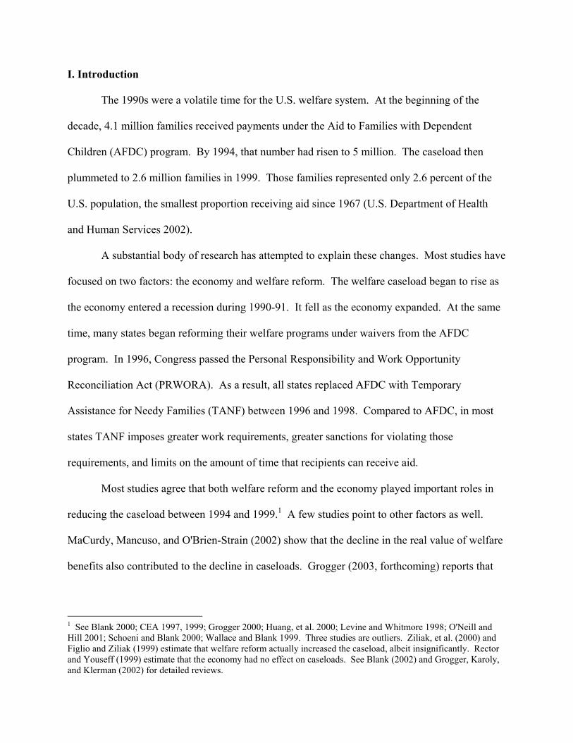
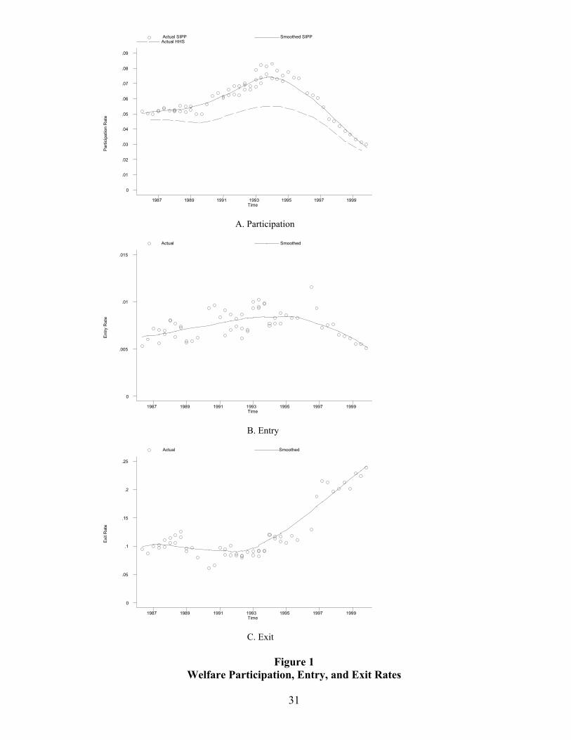
Figure 1 plots trends in welfare use, welfare entries, and welfare exits. In each figure, the

dots represent means by wave within panels.6 Because many of the panels overlap, there are

multiple data points for many time periods. The solid line in each figure represents a lowess

smooth of the raw wave-by-panel averages.

In panel A, I also plot population welfare participation rates based on administrative data

published by the U.S. Department of Health and Human Services (2002). Because the

denominator for the administrative data is the U.S. population, whereas the denominator for the

SIPP series consists only of low-skill women, one would expect the SIPP series to be higher.

What Figure 1 shows is that, for most of the sample period, the general pattern in the SIPP tracks

the administrative data quite well. Welfare use was roughly constant in the late 1980s, rose

sharply between 1990 and 1993-94, and fell sharply thereafter. However, at the end of the

sample period, welfare use fell faster in the SIPP than in the administrative data. This may be

due to under-reporting of welfare use, which increased during the 1990s (Bavier 1999).

Three points are apparent in the plot of entry rates in panel B. First, entry rose from the

mid-1980s to the mid-1990s, then fell in the late 1990s. Thus changes in entry were responsible

for part of the decline in welfare use. Based on both a somewhat different SIPP sample and

administrative data from California, Grogger, Haider, and Klerman (2003) estimate that the

decline in entry may have accounted for about half of the decline in welfare use.

5 The sample also excludes women living in 19 small states. Nine of those states are not separately identified in the SIPP, which precludes me from merging on state-level data. Sample sizes in the other states were so small that, for at least one of the transition models below, there were no actual transitions. With state dummies in the model, this caused the logit model to fail to converge. 6 All SIPP-based estimates in this paper are based on weighted data.

7

It is also apparent that welfare entry is a rare event, even among low-skill women. On

average, less than 1 percent of such women begin a welfare spell in each wave. Furthermore,

entry is volatile. The rarity and volatility of entry rates may help explain why previous estimates

of the effects of welfare reform on welfare entry have been so mixed.

Exit rates are plotted in Panel C. Until about 1993, exit rates were roughly constant at

about 10 percent per wave. By 1999, they had risen to almost 25 percent.

Underlying these exit and entry rates are the welfare spells and non-welfare spells,

respectively, that are the basis for the analysis below. The SIPP samples from the population of

such spells in two distinct ways. The distinction has important implications for the regression

analysis to follow.

Implicitly, the SIPP employs both interval and point sampling of welfare spells. Under

interval sampling, the analyst fixes an observation period and samples spells that begin during

that period. Spells that begin during the panel period are essentially interval sampled. For the

remainder of the paper, I refer to these as "fresh" spells. Under some fairly standard

assumptions, such fresh spells are representative of the population distribution of spells (Cox

1967; Frank 1978).

Under point sampling, the analyst samples from spells in progress at a point in time. This

is essentially how the SIPP samples spells that are in progress when the panel begins. I refer to

these as "ongoing" spells for the remainder of the paper. These ongoing spells are representative

of spells in progress as of month 1 of the panel, but they are not representative of the population

distribution of spells. They over-represent lengthy spells and longer-term recipients, who are

generally more disadvantaged than the average recipient (Bane and Ellwood 1994).

8

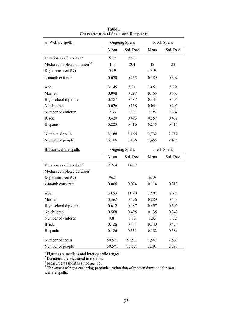
These differences are apparent in Table 1, which provides summary characteristics of

spells and recipients sampled under the two different mechanisms. To compute the duration of

ongoing spells, I use data on the date the spell began that is reported in the SIPP recipiency

history module.7 Column (1) of Panel A shows that the average ongoing welfare spell had been

in progress for 62 months as of month 1 of the panel. The median completed duration of these

spells is 160 months, which is due to the high level of right-censoring among those spells.8 The

median completed duration for fresh spells is 12 months, as shown in column (2). The average

exit rate from the ongoing spells is only 0.07, compared to 0.189 from the fresh spells.

The Table also shows that welfare recipients differ in a number of important ways across

the two types of spells. Recipients experiencing ongoing spells are older, less likely to be

married, less educated, have more children, and are more likely to be minority members than

their counterparts experiencing fresh spells. Other studies have also associated these traits with

longer spells on aid (Bane and Ellwood 1983, 1994; O'Neill et al. 1987; Pavetti 1993).

The information in Panel A illustrates clearly that the spells and recipients sampled by the

two different mechanisms are substantially different. Given these differences, it would not be

surprising if the two groups of recipients responded differently to policy interventions or changes

in economic conditions. To account for this possibility, I stratify the sample in the analysis that

follows, estimating separate exit regressions from the fresh and ongoing welfare spells. The

fresh spells yield estimates relevant to the population distribution of spells, whereas the ongoing

7 Ongoing spells are spells in progress in month 1 of the panel for which the respondent provided a start date that preceded month 1. Spells in progress in month 1 that were reported to start in month 1 or later are classified as fresh spells. Preliminary life table analyses showed that exit rates for these spells did not differ significantly from fresh spells that began after the first wave. 8 Non-censored ongoing spells had a mean month-1 duration of 55 months and a mean completed duration of 72 months.

9

spells provide insights into how the changes that occurred during the 1990s affected longer-term

welfare recipients.

The non-welfare spells that underlie the entry analysis are also implicitly sampled by the

same two mechanisms. The ongoing non-welfare spells are primarily initial non-welfare spells,

that is, they pertain to people who have never received welfare. The fresh non-welfare spells

begin when welfare spells end during the panel period, and thus are useful for studying re-entry.

Given the discussion above, it would seem natural to explicitly distinguish the initial

spells from other ongoing non-welfare spells. However, the SIPP does not allow one to make

such a distinction consistently throughout the sample period. Prior to the 1996 panel, the

recipiency history module asked all SIPP respondents whether they had received aid at any point

prior to the beginning of the panel. In the 1996 panel, those questions were posed only to

recipients not receiving aid in month 1. Thus in the 1996 panel, initial spells cannot be

distinguished from other ongoing non-welfare spells. A tabulation of the pre-1996 data shows

that 95 percent of ongoing non-welfare spells are indeed initial spells. As a result, I refer to the

analysis of the ongoing non-welfare spells as the initial entry analysis below.

Not surprisingly, Panel B of Table 1 shows that the non-welfare spells and potential

recipients sampled according to the two different mechanisms are quite different. Median

completed durations could not be computed for either type of spell due to high rates of right-

censoring. Beyond that, only 0.6 percent of low-skill women begin an initial spell each wave; in

contrast, 11 percent of former recipients re-enter. Those re-entering are younger, less likely to be

married, less educated, have more children, and are more likely to be minority members than

those at risk of initial entry. As with the exit analysis, I stratify the non-welfare spells for the

entry analysis below.

10

B. Economic and Policy Variables

I merge the welfare transition data described above to several variables intended to

characterize the economic conditions and policy environment facing actual and potential welfare

recipients. Economic conditions are captured by two variables: the unemployment rate and the

25th percentile weekly wage. Both measures vary by state of residence and year.

Unemployment data are published by the Bureau of Labor Statistics (2002). The weekly wage

measure is based on tabulations of the Outgoing Rotation Groups of the Current Population

Survey from MacRae (2002).

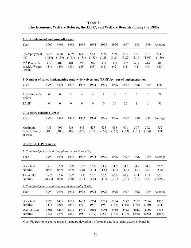
Annual means are presented in the first panel of Table 2. Average unemployment rose

quickly in the early 1990s and then fell gradually. Low-skill wages fell about 6 percent between

1990 and 1994, remained roughly constant through 1997, then returned to their 1990 level by

1999.

Welfare reform is represented by two dummy variables. The first equals one in all

months between the time that the recipient's state of residence implements a statewide welfare

reform waiver and the time that it implements its TANF plan. The second equals one in all

months after it implements its TANF plan. These data are from Council of Economic Advisers

(1999). The second panel of Table 2 shows that states began implementing state-wide waivers in

1992. By the time PRWORA was passed, 29 states had implemented some sort of state-wide

waiver. Twenty-four states implemented TANF during 1996; all but one of the rest put their

TANF plans in place during 1997.9

These variables allow me to estimate the effects of reform as a whole, but they do not

allow me to estimate the effects of specific reforms such as work requirements, sanctions, and

time limits. As valuable as such estimates might be, preliminary analyses revealed that it was 9 The District of Columbia is treated like a state both here and below.

11

impossible to estimates the effects of specific reforms on transition rates with any precision, even

with the sample sizes available in the SIPP. As a result, I follow the lead of much of the prior

literature on welfare reform, providing estimates of the effects of waivers and TANF as a bundle.

The other welfare policy variable is the maximum benefit available to a family of three.

The maximum payment varies dramatically across states, from $170 in Mississippi to $626 in

California and $1,118 in Alaska (in 1999). Panel C of Table 2 shows that the real value of

average benefits fell by nearly 20 percent over the 1990s.

The final policy variable in the models below reflects the generosity of the EITC. The

federal EITC is a refundable credit that can be characterized by its initial subsidy rate, its

maximum credit (or equivalently, the income threshold below which the subsidy is available),

the threshold at which the credit is phased out as earnings increase, and the phase-out rate.10

Fifteen states have implemented EITC's of their own, which typically increase the subsidy rate

(and maximum payment) by either a fixed amount or a proportion of the federal rate.

Panel D of Table 2 presents mean subsidy rates and maximum benefits by year of the

combined federal and state EITC's.11 Two major changes occurred during the 1990s. First, the

program became more generous. The credit rate for one-child families rose from 14.1 percent in

1990 to 34.8 percent in 1999. At the same time, the maximum credit rose from $1,196 to $2,314.

Second, the program became relatively more generous for larger families. Credit rates and

maximum credits were essentially the same for all families in 1990. In 1999, the credit rate was

6.4 percentage points, or 18 percent, higher for families with multiple children than for families

with a single child. The maximum credit was $1500 higher. In the models reported below, I use

10 See Hotz and Scholz (2001) for a useful summary of the program. 11 The credit rate used in the regressions is the sum of the federal and refundable state credit rates. Results based on measures that included non-refundable state credits were somewhat weaker, which may be the result of measurement error. For workers with little tax liability, the nominal non-refundable credit rate may substantially overstate the actual credit rate facing the worker.

12

the combined state and federal credit rate to characterize the generosity of the EITC. Estimates

based on the maximum credit were generally similar but in some cases were less significant.

III. Estimation

Since the spells are measured discretely, it is natural to use a discrete-time hazard model

for the regression analysis. Since entries represent a transition from a non-welfare spell to a

welfare spell, and exits represent a transition from a welfare spell to a non-welfare spell, I can

write the transition hazard generically as:

)1(]);([)1 by wave tionednot transi hadfamily |spell of th wavein ns transitiofamily ()(

stdist

idgXZF

ddiPdhεθδγ +++=

−=

The vector Zst represents the economic and policy variables discussed above, including

the unemployment rate, the 25th percentile wage, the waiver and TANF dummies, welfare

benefits, and the EITC credit rate. These variables vary only by state and year, with the

exception of the EITC credit rate, which also varies by family size. The vector Xid represents

individual characteristics such as age, education, race, marital status, number of children, and the

age distribution of children. Most of these variables are time-varying.

The term ),( θdg is the baseline hazard, reflecting how the conditional transition rate

varies with the length of the spell. For the exit and the re-entry models, the baseline hazard is

specified flexibly via a series of dummy variables that capture durations of different intervals.

The intervals reflect durations over which the hazard is roughly constant, a revealed by some

preliminary analyses.12 In the initial entry model, durations are collinear with age.13 Thus age

12 For the fresh spells (both welfare and non-welfare), separate dummies are included for durations of 1 to 7 waves; the hazard is assumed to be constant thereafter. For the ongoing welfare spells, separate dummies are included for durations of 1 to 3 waves; another is included for durations of 4 to 5 waves; the hazard is assumed to be constant thereafter. 13 In principle, one could use information from the recipiency history modules from the pre-1996 to measure the duration since the last welfare spell for persons who had previously been on aid. Since the information needed to

13

was entered via a series of dummy variables to provide a flexible baseline hazard for this

model.14

The final term εst represents unobservable, state-specific factors that influence welfare

transitions. Examples may include unmeasured aspects of the state's economy or political

sentiment toward welfare programs.

A problem arises if εst is correlated with the variables included in Zst. Such correlation

has been referred to as policy endogeneity in the welfare reform literature. The problem is that,

if the policies reflected in Zst are themselves influenced by unobservable determinants of welfare

transition rates, then estimates based on the hazard model in equation (1) may be biased.

Although there is no way to control for arbitrary forms of policy endogeneity, state and

year dummies may help reduce any potential bias. This amounts to assuming that

sttsst νταε ++= , where sα represents time-invariant characteristics of states that influence

welfare transitions, and tτ represents time-varying unobservables that influence welfare

transitions in a similar manner across the states. The state-specific factors can be controlled for

by including state dummies, or state fixed-effects, in the model, and the time-varying factors can

be controlled for by including year dummies, or period effects. If stν is uncorrelated with Zst,

then the estimates from equation (1) should be consistent.

A convenient choice for the function F( ) is the logistic. With this choice, the transition

models can be estimated with conventional logit regression software. Estimates based on the

logit model are reported in the next section.

construct this variable is unavailable in the 1996 panel, the resulting measure would incorporate measurement error that was correlated with many of the variables of interest. 14 These controls include dummies for single years of age from 15 to 24 and five-year age-group dummies thereafter.

14

IV. Estimation Results

A. Main Estimates

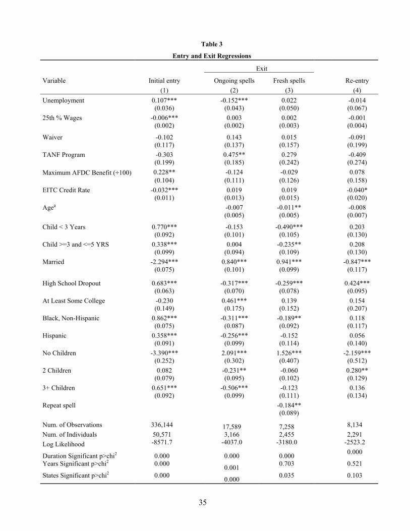
Table 3 presents estimation results. One feature of the logit model is that the estimated

coefficients can be interpreted as approximate proportionate derivatives, where the

approximation is better, the smaller the transition rate. The approximation is likely to be best for

the initial entry model, but for the sake of expositional convenience, I will refer to the estimates

from all the models as if they represented proportionate changes in the transition rates associated

with a one-unit change in the explanatory variables.

Results from the initial entry model are presented in column (1). Both the economic

variables are significant and perform as one might expect. Higher unemployment increases

initial entry. This is consistent with estimates by Gittleman (2001) and Klawitter, Plotnick, and

Edwards (2000), which appear to be the only two prior studies to have focused on initial entries.

The estimate indicates that each percentage-point increase in the mean unemployment rate

increases the rate of initial welfare entry by about 11 percent. Based on the annual means in

Panel A of Table 2, reductions in the unemployment rate should have reduced welfare entry from

1992 to the end of the sample period in 1999.

Higher wages also decrease entry, but their effect is not as great as that of the

unemployment rate. The coefficient indicates that each $10 increase in the real wage reduces

entry by 6 percent. Furthermore, the effects of wages and the unemployment rate worked in

opposite directions over part of the sample period. Based on the annual means in Table 2 and the

wage coefficient in Table 3, wages should have increased initial entry by about 14 percent

between 1990 and 1994, then decreased it by the same amount between 1997 and 1999.

15

The welfare reform coefficients are both negative, as one might expect, with the effect of

TANF substantially larger than the effect of waiver-based reform. The TANF coefficient is

fairly sizeable, indicating that it reduced entry rates about 30 percent. However, its standard

error is also sizeable, which may stem from the collinearity between the TANF variable and the

year dummies. As a result, the estimate is at best only marginally significant, with a t-statistic of

-1.5.

Welfare benefits, in contrast, have a significant positive effect on initial entry. One

would expect higher benefits to increase initial entry, if for no other reason than the higher

eligibility thresholds that they imply. Yet both Gittleman (2001) and Klawitter et al. (2000)

report that higher benefits decrease initial entry, significantly so in the case of Klawitter, et al.

The coefficient in column (1) of Table 3 indicates that a $100 increase in real benefits increases

the initial entry rate by roughly 23 percent. Thus the $89 decline shown in Table 2 would have

reduced initial entry rates by about 20 percent between 1990 and 1999, all else equal.

The EITC coefficient is also significant. Indeed the expansion of the 1990s appears to

have had a strong effect on initial entry rates. The coefficient indicates that each percentage-

point increase in the credit rate reduces initial entry by 3.2 percent. Thus the increase in the

mean credit rate for multiple-child families between 1993 and 1999 would have decreased initial

entry by more than half. With an effect of that magnitude, one might expect the EITC to explain

a substantial portion of the decline in the welfare participation rate over the same period.

The remaining estimates in column (1) show how various demographic characteristics

affect initial entry. These effects largely accord with expectations. Young children, the lack of a

high school diploma, minority status, and the presence of three or more children raise the

likelihood of initial entry. Being married or childless greatly reduces the likelihood of initial

16

entry. This comes as no surprise; married couples have to satisfy more stringent eligibility

conditions than single parents, and the only childless adults who can qualify for aid are women

beyond their first trimester of pregnancy.

Results from the exit models appear in the next two columns. For the most part, exits are

less responsive than initial entries to both economic conditions and policy changes. An

exception is the effect of unemployment on exits from ongoing spells. The estimate indicates

that each percentage-point decline in the unemployment rate should have increased exits from

ongoing spells by about 15 percent. However, unemployment has no effect on fresh spells.

Wages have no significant effect on spells of either type.

The waiver and TANF coefficients are all positive and the two TANF coefficients are

larger than the respective waiver coefficients. However, only the TANF coefficient in the

ongoing spells model is significant. That coefficient is substantial in magnitude, indicating that

TANF increased exit rates by roughly 48 percent.

The maximum benefits coefficients are both negative, suggesting that higher benefits

reduce exit rates. However, both coefficients are insignificant. This is a common finding in

previous studies, including those based on pre-reform data.15 The EITC coefficients are positive

in both models, suggesting that higher credit rates increase exit. Again, however, both

coefficients are insignificant. The demographic variables mostly have significant coefficients,

and most of them accord with expectation.

The final column presents estimates from the re-entry model. Of the variables that

measure the economic and policy environment, only the EITC coefficient is significant,

indicating that increases in the credit rate reduce re-entry. As in the initial entry model, the

15 See Acs, et al (2001), Gittleman (2001), Harris (1993), and Pavetti (1993). Hutchens (1981), O'Neill, et al. (1987) and Ribar (2002) report significant negative effects.

17

welfare reform coefficients are fairly sizable though insignificant. Re-entry seems much less

responsive to economic conditions than initial entries, and less responsive than exits as well.

To summarize, initial entries are most significantly affected by economic conditions,

benefit levels, and the EITC. This suggests that the immediate economic opportunities facing

potential entrants play an important role in determining whether they apply for welfare. Exits are

most significantly affected by the unemployment rate and TANF. Indeed, the only significant

effect of TANF is to increase exits from ongoing spells. The estimated coefficient suggests that

TANF induced longer-term recipients to leave the rolls in substantial numbers. Re-entry seems

to be completely unaffected by economic conditions and benefit levels. The effects of reform on

re-entry are roughly as large (in absolute value) as their effects on exit, but the coefficients are

insignificant. Only the EITC expansions significantly affect re-entry.

In this summary interpretation of the estimates, precision is an issue. The TANF

coefficients in the entry models are sizeable but insignificant. The same is true of the EITC

coefficients in the exit models. It may be that both policies had substantial effects on both

entries and exits. However, even with the sample sizes available in the SIPP, there is insufficient

precision to distinguish some potentially important effects from effects that are equal to zero.

B. Additional Estimates

Table 4 presents estimates from specifications that include additional measures of

economic conditions, including lagged unemployment and job growth. The motivation for these

specifications is that the unemployment rate and the low-skill wage measure might not

adequately control for the state of the economy by themselves, and that adding additional

measures might provide greater insight in to the role played by the economy in influencing

18

entries and exits. In Table 4, only the coefficients associated with the economic and policy

variables are shown in order to save space.

None of the lagged unemployment coefficients are significant. In many previous studies

of the welfare caseload, lagged unemployment often has stronger effects than current

unemployment, and in the case of multiple lags, often the last lag is the only significant

coefficient (CEA 1997, 1999; Figlio and Ziliak 1999; Ziliak, et al. 2001). Klerman and Haider

(2002) argue that such results are indicative of misspecified dynamics and predict that such

patterns should not appear in models of welfare transitions.

Whether that prediction is borne out by these data is a matter of interpretation. In some

cases, the lagged unemployment coefficients are slightly larger than the current coefficients; in

others they are smaller. Testing Klerman and Haider's prediction is hampered by the

considerable collinearity between past and current unemployment, which is also the likely reason

why the current unemployment rate is insignificant when the lag is included in the model.

The job growth coefficients suggest that greater growth increases welfare entry and

decreases welfare exit. However, in all cases, the coefficients are insignificant.

On the whole, these additional measures do not substantially improve the characterization

of the economic conditions affecting welfare transitions. Of all the measures considered, only

current unemployment and low-skill wages significantly affect entry or exit. Furthermore,

except as noted above, including the additional measures in the regression models has little effect

on the other parameter estimates.

V. Decomposing the Effects of Economic and Policy Changes on the Decline in Welfare Participation The coefficients in Table 3 provide quantitative estimates of the effects of economic and

policy changes on welfare transition rates. From these one can infer the qualitative effects of

19

those changes on the welfare participation rate. However, it would be valuable to provide

quantitative information about the effects of recent changes on welfare participation. Although

there are in principle a number of ways one could do this, a common practice in the welfare

reform literature has been to decompose the decline in the welfare participation rate that took

place during the 1990s into components attributable to the expanding economy, welfare reform,

and other factors. I provide such decompositions based on the models presented in Table 3 in

this section.

The basis for these decompositions is the relation:

tt

tt z

zs

s ∆∂∂

≅∆ (2)

where st denotes the welfare participation rate at time t and ∆ denotes a finite change. Equation

(2) says that the change in st due to a change in some factor z (such as the unemployment rate) is

approximately equal to the derivative of st with respect to zt, multiplied by the change in zt. The

approximation is better, the smaller is the change in zt.16

The welfare participation rate can be written in terms of welfare transition rates using the

transition rule:

)1()1( 11 −− −+−= ttttt sesxs , (3)

where et denotes the entry rate and xt denotes the exit rate. In words, equation (3) says that the

welfare participation rate at period t is equal to the welfare participation rate at period t-1, less

exits (1-xt), plus entries (from the proportion 1-st-1 of the population at risk of entry). Because

current participation depends on past participation as well as current transition rates, the

16 For this reason, I compute the decompositions as the sum of several wave-by-wave changes, rather than a single six-year change.

20

participation rate exhibits inertia: current changes in entry and exit rates affect not just the

current participation rate, but future participation rates as well.

To write entry and exit rates in terms of regression models presented in Table 3, I re-

write the entry rate as

ftt

ottt ewewe )1( −+= , (4)

where ote is the entry rate from ongoing non-welfare spells at time t and f

te is the entry rate

from fresh non-welfare spells at time t. Of the sample at risk of entry at time t, wt is the fraction

at risk of entry from ongoing non-welfare spells, so 1-wt is the fraction at risk of entering from

fresh non-welfare spells. Adopting analogous notation, I re-write exit rates as:

ftt

ottt xvxvx )1( −+= . (5)

Substituting (4) and (5) into (3) and differentiating with respect to zt yields:

)1]()1([])1([ 11 −− −∂∂

−+∂∂

+∂∂

−+∂∂

−=∂∂

tt

ft

tt

ot

ttt

ft

tt

ot

tt

t sze

wze

wszx

vzx

vzs

. (6)

Since the transition rates are assumed to be logistic, the derivatives in (6) take the simple

form:

jz

jt

jt

t

jt xx

zx

γ)1( −=∂∂

j=o, f (7)

and

jz

jt

jt

t

jt ee

ze

β)1( −=∂∂

j=o, f (8)

where the term ozγ denotes the coefficient on z in the model for ongoing welfare spells, f

zγ

denotes the coefficient on z in the model for fresh welfare spells, and ozβ and f

zβ denote the

21

corresponding coefficients from the models for ongoing and fresh non-welfare spells.

Substituting (7) and (8) into (6) and the result into (2) provides a formula for decomposing the

decline in the welfare participation rate into components attributable to the economy, welfare

reform, and other factors. In addition to providing an overall decomposition, equation (6) also

provides a means for isolating the contribution of entry and exit to the overall change. The first

term in equation (6) (multiplied by ∆zt) provides the change in the welfare participation rate that

is due to the effect of zt on welfare exits; the second term provides the change in the participation

rate that is due to the effect of zt on welfare entries.

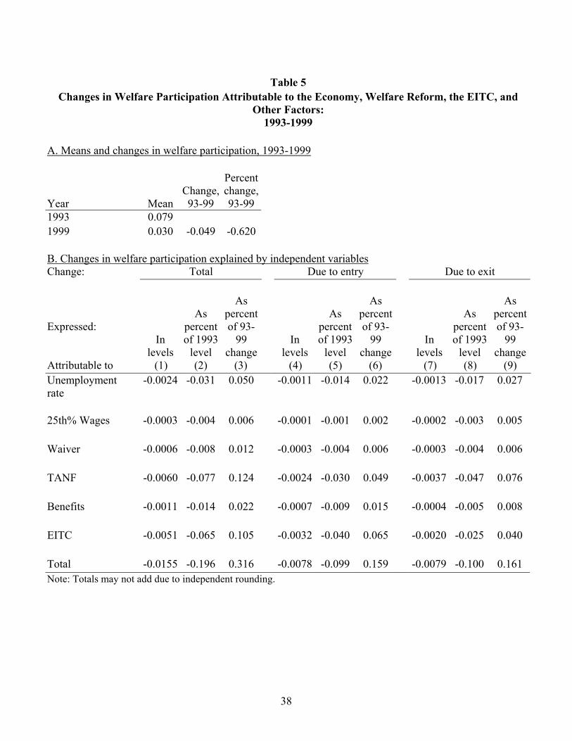
Table 5 presents decompositions for the period from 1993, when the welfare participation

rate peaked, to 1999. The top panel of the Table shows that the peak welfare participation rate

was 7.9 percent. By the end of 1999, it had fallen to 3 percent, a 62 percent decline.

Panel B decomposes this decline into components attributable to economic conditions

and policy changes. The first column presents changes in the participation rate. The second

presents these changes relative to the baseline 1993 participation rate, whereas the third column

presents changes relative to the 1993-1999 decline. Relative to the baseline, the change in the

unemployment rate between 1993 and 1999 reduced the welfare participation rate by 3.1 percent,

which amounts to 5 percent of the 1993-1999 decline in the participation rate.17 Low-skill

wages, which rose only about 5 percent over this period, account for a negligible fraction of the

decline in welfare.

Likewise, welfare waivers account for little of the decline. In contrast, TANF had

sizeable effects on welfare participation. TANF reduced welfare participation by 7.7 percent,

17 Klerman and Haider (2002) have argued that decompositions that start with the peak in welfare use may understate the effect of the economy, because the economy began to improve before the caseload began to fall. When I start the decomposition at the time that the unemployment rate peaks, the change in the unemployment rate accounts for about 9 percent of the caseload decline, with little change in the other results.

22

relative to baseline, accounting for 12.4 percent of the 1993-1999 decline. Welfare benefits had

a small effect, accounting for just over 2 percent of the decline in the participation rate.

Like TANF, the EITC expansions had substantial effects on the welfare participation rate.

They reduced welfare participation by 6.5 percent, relative to its 1993 peak. Thus they

accounted for over 10 percent of the 1993-1999 decline.

Columns (4) through (6) show the components of the change in the welfare participation

rates that are due to changes in entry; columns (7) through (9) show the components that are due

to changes in exit. These figures show that the effects of the EITC and welfare benefits worked

primarily through entries. The effects of TANF worked mostly through exits, whereas the effect

of the unemployment rate worked similarly through both.

In total, the six economic and policy factors accounted for in the decompositions combine

to generate a roughly 20 to 25 percent decline in the welfare participation rate. Put differently,

they account for less than half of the decline that took place during the 1990s. The remainder is

explained by factors other than the falling unemployment rate and the changes in welfare and tax

policy accounted for in the model. These results make it clear that the decline in welfare

participation was a very complex phenomenon. Neither the longest economic expansion in post-

war history, nor the greatest change in social policy since the Great Depression, explains more

than a fraction of the decline.

Before moving on, it is worth noting that these decompositions are similar to those in

Grogger (2004, forthcoming). There I estimated that welfare reform explained about 14 percent

of the 1993-1999 decline in welfare participation, the EITC explained about 16 percent, and the

unemployment rate explained about 10 percent. The similarity of my earlier estimates to those

presented here is striking because the earlier estimates were based on an analysis of welfare

23

participation rates in the Current Population Survey. Despite the use of different data sets and

different analytical techniques, both analyses attribute similar portions of the caseload decline to

changes in the economy and changes in policy.18

VI. Predicting the Effects of the Recent Economic Slowdown

The equations that underlie the decomposition analysis above can also be used to predict

how welfare participation rates should respond to the recent downturn in the economy. Between

January 2000 and September 2002, the U.S. unemployment rate rose from 4.0 to 5.6 percent.

Yet at the same time, the welfare caseload has actually fallen slightly, from an average of 2.27

million families during 2000 to 2.02 million families in June 2002 (U.S. Department of Health

and Human Services, 2002). Predictions based on the models in Table 3 help explain why

caseloads have remained roughly constant despite the increase in unemployment.

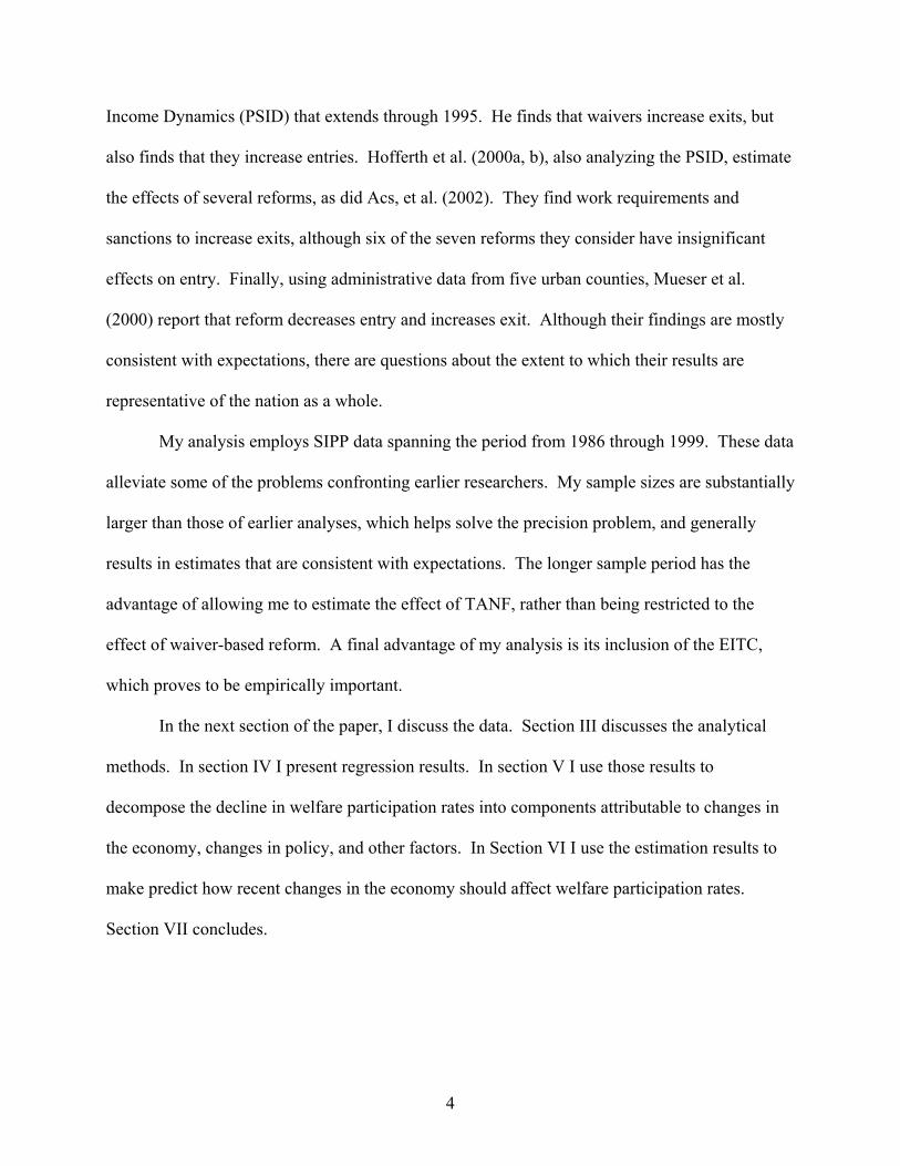
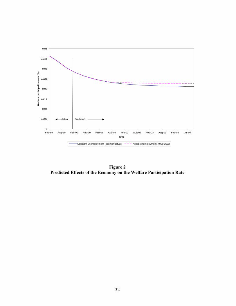
I use equation (3) above to generate two sets of out-of-sample predictions for the welfare

participation rate. The first is a counterfactual, which provides a prediction of how the

participation rate would have evolved if the unemployment rate had remained at its January 2000

value of 4.0 percent. The result is displayed as the solid line in Figure 2. It shows that there was

a fair amount of inertia in the system as of the beginning of 2000. Even if the unemployment

rate had remained constant, the increase in exit rates and decrease in entry rates that took place

18 At the same time, my decomposition results differ markedly from those of Haider, Klerman, and Roth (2002). Based on California transition data, they conclude that the economy accounted for roughly half of the decline in that state's caseload. Although differences in data and methods may explain part of the difference between their analysis and mine, there are many reasons to think that California should be different than the nation as a whole. California's main pre-PRWORA welfare waiver increased earnings disregards and reduced the implicit tax rates on earnings, policy changes that should have actually increased its caseload, all else equal. The state was the last to implement its TANF plan, in January 1998. It has a relatively lenient sanction policy and adult-only time limits. Compared to the rest of the nation, one would expect welfare reform to have played a relatively small role in reducing California's caseload. Furthermore, the recession of the early 1990s cut deeper and lasted longer in California than in the nation as a whole. Once it recovered, the state's economy grew more vigorously than elsewhere as well. For all these reasons, one would expect the economy to explain more of the caseload decline in California than in the nation as a whole.

24

during the latter part of the sample period (see Panels A and B of Figure 1) would have led to

continued declines in the welfare participation rate.

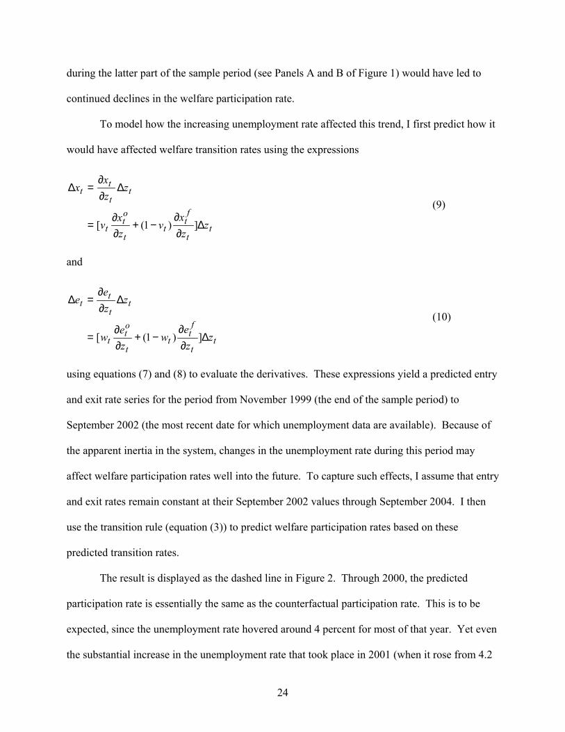
To model how the increasing unemployment rate affected this trend, I first predict how it

would have affected welfare transition rates using the expressions

tt

ft

tt

ot

t

tt

tt

zzx

vzx

v

zzx

x

∆∂∂

−+∂∂

=

∆∂∂

=∆

])1([

(9)

and

tt

ft

tt

ot

t

tt

tt

zze

wze

w

zze

e

∆∂∂

−+∂∂

=

∆∂∂

=∆

])1([

(10)

using equations (7) and (8) to evaluate the derivatives. These expressions yield a predicted entry

and exit rate series for the period from November 1999 (the end of the sample period) to

September 2002 (the most recent date for which unemployment data are available). Because of

the apparent inertia in the system, changes in the unemployment rate during this period may

affect welfare participation rates well into the future. To capture such effects, I assume that entry

and exit rates remain constant at their September 2002 values through September 2004. I then

use the transition rule (equation (3)) to predict welfare participation rates based on these

predicted transition rates.

The result is displayed as the dashed line in Figure 2. Through 2000, the predicted

participation rate is essentially the same as the counterfactual participation rate. This is to be

expected, since the unemployment rate hovered around 4 percent for most of that year. Yet even

the substantial increase in the unemployment rate that took place in 2001 (when it rose from 4.2

25

percent in January to 5.8 percent in December) is predicted to have little effect on the welfare

participation rate that year. This is the result of the inertia in the system: changes in

unemployment affect welfare transition rates contemporaneously, but those changes take time to

affect the welfare participation rate. This is the implication of the transition rule in equation (3),

by which the participation rate is a function of past participation as well as current transition

rates. This inertia helps to explain why the caseload continued to decline slightly between 2001

and mid-2002, even as the economy deteriorated substantially.

Another part of the explanation is that the unemployment rate has a fairly small effect on

the participation rate. The predicted participation rate for September 2003, after twelve months

of assumed 5.6 percent unemployment, is 0.023. The counterfactual prediction, based on the

assumption that unemployment remained constant at 4.1 percent after November 1999, is 0.022.

Although unemployment has statistically significant effects on transition rates, as shown in Table

3, its quantitative effect on the participation rate is fairly small, as was suggested by the

decomposition analysis in Table 5.

VII. Conclusions

The results from this study are consistent with those from much of the prior literature on

welfare reform. Both the economy and reform played important roles in reducing the welfare

caseload during the late 1990s. The EITC had particularly strong effects.

At the same time, decomposing welfare participation into entries and exits yields insights

not forthcoming from studies of the welfare caseload. It shows that much of the decline in

welfare participation during the 1990s was driven by a reduction in welfare entries. First-time

entry, in turn, was affected by the improving state of the economy, the decline in real benefit

levels, and the expansion of the EITC.

26

Higher exit rates also drove the caseload decline. Exit rates fell due to the decline in

unemployment and the imposition of TANF. TANF had a particularly important effect on long-

term welfare spells.

The decomposition analysis indicated that TANF and the EITC played the most

important roles in reducing welfare caseloads during the 1990s. The economy also played a part,

but its part was smaller. The relatively modest effect of the economy, in conjunction with inertia

in the caseload, helps explain why welfare receipt has remained roughly constant recently,

despite considerable increases in unemployment.

The initial entry results raise a number of issues. First, there is the question of whether

TANF has reduced entries. The estimated effects are large, but they are statistically

insignificant. The sizeable and significant EITC effects would be generally regarded as

beneficial. At the same time, they raise questions about the take-up of safety-net services. If

most families learn about such services when they first apply for welfare, then declines in initial

entry rates due to expansions of the EITC may reduce knowledge and take-up of non-cash

transfers.

More generally, the initial entry effects raise the question of how welfare reform has

affected the behavior and well-being of families that would have signed up for welfare in the

absence of recent policy changes. Although numerous experiments provide information about

the effects of welfare reform on families receiving aid, non-entrants are inherently more difficult

to study than recipients. Nevertheless, since roughly half the decline in the caseload was due to

decreases in entry, the question merits serious attention.

27

References

Acs, Gregory, Katherin Ross Philips, Caroline Ratcliffe, and Douglas Wissoker, “Comings and Goings: The Changing Dynamics of Welfare in the 1990s,” unpublished manuscript, Washington, DC: Urban Institute, 2001.

Bane, Mary Jo, and David Ellwood, "The Dynamics of Dependence: The Routes to Self-Sufficiency," Manuscript, Urban Systems Research and Engineering, June 1983.

Bane, Mary Jo, and David Ellwood, Welfare Realities: From Rhetoric to Reform, Cambridge, MA: Harvard University Press, 1994.

Bavier, Richard. "An Early Look at the Effects of Welfare Reform." Mimeo, Office of Management and Budget, March 1999.

Blank, Rebecca M., “Analyzing the Length of Welfare Spells,” Journal of Public Economics, Vol. 39, No. 3, August 1989, pp. 245-273.

Blank, Rebecca M., “Evaluating Welfare Reform in the United States,” Journal of Economic Literature, forthcoming.

Blank, Rebecca M., “What Causes Public Assistance Caseloads to Grow?” Journal of Human Resources, Vol. 36, No. 1, Winter 2001.

Blank, Rebecca M., and Patricia Ruggles, “When Do Women Use AFDC and Food Stamps? The Dynamics of Eligibility versus Participation,” Journal of Human Resources, Vol. 31, No. 1, Winter 1996, pp. 57-89.

Boskin, Michael J., and Frederick C. Nold, "A Markov Model of Turnover in Aid to Families with Dependent Children," Journal of Human Resources, Vol. 10, No. 4, Autumn 1975, 467-481.

Council of Economic Advisers (CEA), Explaining the Decline in Welfare Receipt, 1993-1996, Washington, DC, May 1997.

Council of Economic Advisers (CEA), The Effects of Welfare Policy and the Economic Expansion on Welfare Caseloads: An Update, Washington, DC, August 1999.

Cox, D.R. (1967) "Some Sampling Problems in Technology." In N.L. Johnson and H. Smith, eds., New Developments in Survey Sampling. New York: Wiley.

Figlio, David N., and James P. Ziliak, “Welfare Reform, The Business Cycle, and the Decline in AFDC Caseloads,” in Sheldon H. Danziger, ed., Economic Conditions and Welfare Reform, Kalamazoo, MI: W. E. Upjohn Institute for Employment Research, 1999, pp. 17-48.

Frank, Robert. (1978) "How Long is a Spell of Unemployment?" Econometrica 46, 285-302.

28

Gittleman, Maury, "Declining Caseloads: What Do the Dynamics of Welfare Participation Reveal?" Industrial Relations, Vol. 40, No. 4, October 2001, 537-570.

Grogger, Jeffrey, “Time Limits and Welfare Use,” Journal of Human Resources, 2004 (forthcoming).

Grogger, Jeffrey, “The Effects of Time Limits, the EITC, and Other Policy Changes on Welfare Use, Work, and Income Among Female-Headed Families,” Review of Economics and Statistics, 2003 (forthcoming).

Grogger, Jeffrey, Steven Haider, and Jacob A. Klerman, "Why Did the Welfare Rolls Fall? The Importance of Entry," American Economic Review, May 2003.

Grogger, Jeffrey, Lynn A. Karoly, and Jacob A. Klerman, Consequences of Welfare Reform: A Research Synthesis. Santa Monica, CA: RAND, 2002. http://www.acf.hhs.gov/programs/opre/welfare_reform/reform_cover.html

Harris, Kathleen M. "Work and Welfare among Single Mothers in Poverty." American Journal of Sociology 99, September 1993, 317-352.

Hofferth, Sandra L., Stephen Stanhope, and Kathleen Mullan Harris, “Remaining Off Welfare in the 1990s: The Influence of Public Policy and Economic Conditions,” Ann Arbor, MI: Institute for Social Research, October 2000a.

Hofferth, Sandra L., Stephen Stanhope, and Kathleen Mullan Harris, “Exiting Welfare in the 1990s: Did Public Policy Influence Recipients’ Behavior,” Ann Arbor, MI: Institute for Social Research, October 2000b.

Hotz, V. Joseph, and John Karl Scholz, "The Earned Income Tax Credit." NBER Working Paper 8078, January 2001.

Hoynes, Hilary W., "Local Labor Markets and Welfare Spells: Do Demand Conditions Matter?" Review of Economics and Statistics, Vol. 83, No. 3, August 2000, 351-368.

Hutchens, Robert M., "Entry and Exit Transitions in a Government Transfer Program: The Case of Aid to Families with Dependent Children," Journal of Human Resources, Vol. 16, No. 3, Spring 1981, 217-237.

Klawitter, Marieka, Robert D. Plotnick, and Mark Evan Edwards, "Determinants of Initial Entry onto Welfare by Young Women," Journal of Policy Analysis and Management, Vol. 19, No. 4, 2000, 527-546.

Klerman, Jacob A., and Steven Haider, “A Stock-Flow Analysis of the Welfare Caseload: Insights from California Economic Conditions,” Santa Monica, CA: RAND, September 2002.

29

Levine, Phillip B., and Diane M. Whitmore, “The Impact of Welfare Reform on the AFDC Caseload,” National Tax Association Proceedings–1997, Washington, DC: National Tax Association, 1998.

MacRae, Duncan, "Work Incentives in Welfare Benefits: An Analysis of the U.S. Case," mimeo, UCLA Department of Political Science, May 2002.

MaCurdy, Thomas, David Mancuso, and Margaret O’Brien-Strain, “How Much Does California’s Welfare Policy Explain the Slower Decline of Its Caseload,” unpublished manuscript, December 2000.

Meyer, Bruce D., and Dan T. Rosenbaum, “Welfare, the Earned Income Tax Credit, and the Labor Supply of Single Mothers,” Quarterly Journal of Economics, Vol. CXVI, August 2001, pp. 1063-1114.

Moffitt, Robert A., “The Effect of Pre-PRWORA Waivers on AFDC Caseloads and Female Earnings, Income, and Labor Force Behavior,” in Sheldon H. Danziger, ed., Economic Conditions and Welfare Reform, Kalamazoo, MI: W. E. Upjohn Institute for Employment Research, 1999, pp. 91-118.

Mueser, Peter R., Julie L. Hotchkiss, Christopher T. King, Philip S. Rokicki, and David W. Stevens, The Welfare Caseload, Economic Growth and Welfare-to-Work Policies: An Analysis of Five Urban Areas, July 2000.

O’Neill, June E.,. Laurie J. Bassi, and Douglas A. Wolf, "The Duration of Welfare Spells," Review of Economics and Statistics, Vol. 69, No. 2, May 1987, 241-247.

O’Neill, June E., and M. Anne Hill, Gaining Ground? Measuring the Impact of Welfare Reform on Welfare and Work, New York, NY: Manhattan Institute for Policy Research, Civic Report #17, July 2001.

Pavetti, LaDonna A., The Dynamics of Welfare and Work: Exploring the Process By Which Women Work Their Way Off Welfare, Ph.D. Dissertation, Harvard University, 1993.

Rector, Robert E., and Sarah E. Youssef, The Determinants of Welfare Caseload Decline, Washington, DC: The Heritage Foundation, Paper # CDA99-04, May 1999.

Ribar, David C. "Transitions from Welfare and the Employment Prospects of Low-Skill Workers," Manuscript, George Washington University, July 2002.

Schoeni, Robert F., and Rebecca M. Blank, “What Has Welfare Reform Accomplished? Impacts on Welfare Participation, Employment, Income, Poverty, and Family Structure,” Cambridge, MA: National Bureau of Economic Research, Working Paper #7627, March 2000.

U.S. Bureau of Labor Statistics, Labor Force Statistics from the Current Population Survey, 2002, www.bls.gov/cps/home.htm.

30

U.S. Department of Health and Human Services, U.S. Welfare Caseloads Information, Washington, DC: Administration for Children and Families, www.acf.dhhs.gov/news/stats/newstat2.shtml, 2001b.

Wallace, Geoffrey, and Rebecca M. Blank, “What Goes Up Must Come Down? Explaining Recent Changes in Public Assistance Caseloads,” in Sheldon H. Danziger, ed., Economic Conditions and Welfare Reform, Kalamazoo, MI: W. E. Upjohn Institute for Employment Research, 1999, pp. 49-89.

Westat. Survey of Income and Program Participation Users' Guide, Third Edition. Washington, DC: U.S. Census Bureau, 2001.

Ziliak, James P., David N. Figlio, Elizabeth E. Davis, and Laura S. Connolly, “Accounting for the Decline in AFDC Caseloads: Welfare Reform or the Economy?” The Journal of Human Resources, Vol. 35, No. 3, January 2000.

31

Parti

cipa

tion

Rat

e

Time

Actual SIPP Smoothed SIPP Actual HHS

1987 1989 1991 1993 1995 1997 1999

0

.01

.02

.03

.04

.05

.06

.07

.08

.09

A. Participation

Entry

Rat

e

Time

Actual Smoothed

1987 1989 1991 1993 1995 1997 1999 0

.005

.01

.015

B. Entry

Exit

Rat

e

Time

Actual Smoothed

1987 1989 1991 1993 1995 1997 1999 0

.05

.1

.15

.2

.25

C. Exit

Figure 1

Welfare Participation, Entry, and Exit Rates

32

0

0.005

0.01

0.015

0.02

0.025

0.03

0.035

0.04

Feb-99 Aug-99 Feb-00 Aug-00 Feb-01 Aug-01 Feb-02 Aug-02 Feb-03 Aug-03 Feb-04 Jul-04

Time

Wel

fare

par

ticip

atio

n ra

te (%

)

Constant unemployment (counterfactual) Actual unemployment, 1999-2002

Actual Predicted

Figure 2 Predicted Effects of the Economy on the Welfare Participation Rate

33

Table 1 Characteristics of Spells and Recipients

A. Welfare spells Ongoing Spells Fresh Spells

Mean Std. Dev. Mean Std. Dev.

Duration as of month 12 61.7 65.3 Median completed duration1,2 160 204 12 28 Right censored (%) 55.9 44.9

4-month exit rate 0.070 0.255 0.189 0.392

Age 31.45 8.21 29.61 8.99 Married 0.098 0.297 0.155 0.362 High school diploma 0.387 0.487 0.431 0.495 No children 0.026 0.158 0.044 0.205 Number of children 2.33 1.37 1.95 1.24 Black 0.420 0.493 0.357 0.479 Hispanic 0.223 0.416 0.215 0.411

Number of spells 3,166 3,166 2,732 2,732 Number of people 3,166 3,166 2,455 2,455

B. Non-welfare spells Ongoing Spells Fresh Spells

Mean Std. Dev. Mean Std. Dev.

Duration as of month 13 216.4 141.7 Median completed duration4 Right censored (%) 96.3 65.9 4-month entry rate 0.006 0.074 0.114 0.317

Age 34.53 11.90 32.04 8.92 Married 0.562 0.496 0.289 0.453 High school diploma 0.612 0.487 0.497 0.500 No children 0.568 0.495 0.135 0.342 Number of children 0.81 1.13 1.83 1.32 Black 0.126 0.331 0.340 0.474 Hispanic 0.126 0.331 0.182 0.386

Number of spells 50,571 50,571 2,567 2,567 Number of people 50,571 50,571 2,291 2,291 1 Figures are medians and inter-quartile ranges. 2 Durations are measured in months. 3 Measured as months since age 15. 4 The extent of right-censoring precludes estimation of median durations for non-welfare spells.

34

Table 2: The Economy, Welfare Reform, the EITC, and Welfare Benefits during the 1990s

A. Unemployment and low-skill wages

Year 1990 1991 1992 1993 1994 1995 1996 1997 1998 1999 Average

Unemployment (%)

5.47 (1.14)

6.48 (1.54)

6.89 (1.61)

6.37 (1.51)

5.68 (1.32)

5.26 (1.28)

5.21(1.24)

4.77(1.22)

4.43(1.19)

4.16 (1.05)

5.47 (1.56)

25th Percentile Weekly Wages (1998$)

412 (51)

407 (49)

401 (50)

396 (48)

389 (43)

391 (41)

390 (42)

392 (41)

405 (42)

414 (40)

400 (45)

B. Number of states implementing state-wide waivers and TANF, by year of implementation

Year 1990 1991 1992 1993 1994 1995 1996 1997 1998 1999 Total

Any state-wide waiver

0 0 3 4 4 8 10 0 0 0 29

TANF 0 0 0 0 0 0 24 26 1 0 51

C. Welfare benefits (1998$)

Year 1990 1991 1992 1993 1994 1995 1996 1997 1998 1999 Average

Maximum benefit, family of three

481 (189)

469 (188)

458 (182)

445 (176)

437 (172)

425 (168)

413 (161)

401 (153)

397 (151)

392 (154)

432 (171)

D. Key EITC Parameters

1. Combined federal and state phase-in credit rate (%)

Year 1990 1991 1992 1993 1994 1995 1996 1997 1998 1999 Average

One-child families

14.1 (0.6)

16.9 (0.7)

17.9 (0.7)

18.7 (0.8)

26.6 (1.1)

34.4 (1.5)

34.6(1.7)

34.5(1.7)

34.9(1.9)

34.8 (2.0)

26.7 (8.6)

Two-child families

14.2 (0.73)

17.6 (0.9)

18.7 (1.0)

19.8 (1.1)

30.5 (1.5)

36.7 (1.7)

40.8(2.1)

40.9(2.1)

41.1(2.3)

41.2 (2.4)

30.1 (10.92)

2. Combined federal and state maximum credit (1998$)

Year 1990 1991 1992 1993 1994 1995 1996 1997 1998 1999 Average

One-child families

1196 (47)

1439(60)

1551(64)

1633 (72)

2264 (94)

2263 (95)

2264(109)

2277(113)

2317 (135)

2314 (140)

1952 (431)

Multiple child families

1201 (62)

1496(79)

1628(86)

1727 (95)

2818 (139)

3369 (157)

3748(191)

3774(197)

3844 (246)

3830 (255)

2743 (1066)

Note: Figures represent means and (standard deviations) of annual state-level data, except in Panel B.

35

Table 3

Entry and Exit Regressions

Exit

Variable Initial entry Ongoing spells Fresh spells Re-entry (1) (2) (3) (4) Unemployment 0.107*** -0.152*** 0.022 -0.014 (0.036) (0.043) (0.050) (0.067) 25th % Wages -0.006*** 0.003 0.002 -0.001 (0.002) (0.002) (0.003) (0.004)

Waiver -0.102 0.143 0.015 -0.091 (0.117) (0.137) (0.157) (0.199) TANF Program -0.303 0.475** 0.279 -0.409 (0.199) (0.185) (0.242) (0.274) Maximum AFDC Benefit (÷100) 0.228** -0.124 -0.029 0.078 (0.104) (0.111) (0.126) (0.158) EITC Credit Rate -0.032*** 0.019 0.019 -0.040* (0.011) (0.013) (0.015) (0.020) Agea -0.007 -0.011** -0.008 (0.005) (0.005) (0.007)

Child < 3 Years 0.770*** -0.153 -0.490*** 0.203 (0.092) (0.101) (0.105) (0.130) Child >=3 and <=5 YRS 0.338*** 0.004 -0.235** 0.208 (0.099) (0.094) (0.109) (0.130) Married -2.294*** 0.840*** 0.941*** -0.847***

(0.075) (0.101) (0.099) (0.117)

High School Dropout 0.683*** -0.317*** -0.259*** 0.424*** (0.063) (0.070) (0.078) (0.095) At Least Some College -0.230 0.461*** 0.139 0.154 (0.149) (0.175) (0.152) (0.207) Black, Non-Hispanic 0.862*** -0.311*** -0.189** 0.118 (0.075) (0.087) (0.092) (0.117) Hispanic 0.358*** -0.256*** -0.152 0.056 (0.091) (0.099) (0.114) (0.140) No Children -3.390*** 2.091*** 1.526*** -2.159*** (0.252) (0.302) (0.407) (0.512) 2 Children 0.082 -0.231** -0.060 0.280** (0.079) (0.095) (0.102) (0.129) 3+ Children 0.651*** -0.506*** -0.123 0.136 (0.092) (0.099) (0.111) (0.134) Repeat spell -0.184** (0.089)

Num. of Observations 336,144 17,589 7,258 8,134 Num. of Individuals 50,571 3,166 2,455 2,291 Log Likelihood -8571.7 -4037.0 -3180.0 -2523.2

Duration Significant p>chi2 0.000 0.000 0.000 0.000

Years Significant p>chi2 0.000 0.001 0.703 0.521

States Significant p>chi2 0.000 0.000 0.035 0.103

36

Notes to Table 3

a - Because age is collinear with the elapsed duration of initial non-welfare spells, it is entered as a series of dummies in the initial entry regression in order to provide a flexible baseline hazard. Notes: Standard errors (in parentheses) account for presence of multiple observations per person In addition to the variables shown, all models include a constant, a dummy for other, non-Hispanic race/ethnicity, and (except for the initial entry regression) a set of elapsed duration dummies. Asterisks indicate significance at 10 percent (*), 5 percent (**), and 1 percent (***).

37

Tab

le 4

E

ntry

and

Exi

t Reg

ress

ions

with

Add

ition

al C

ontr

ols f

or E

cono

mic

Con

ditio

ns

Exit

In

itial

ent

ry

Ong

oing

spel

ls

Fres

h sp

ells

R

e-en

try

Var

iabl

e (1

) (2

) (3

) (4

) (5

) (6

) (7

) (8

)

Une

mpl

oym

ent

0.06

1 0.

134*

**

-0

.112

* -0

.157

***

0.09

1 0.

007

-0.0

26

0.02

6

(0.0

50)

(0.0

41)

(0

.065

) (0

.047

) (0

.071

) (0

.054

) (0

.094

) (0

.072

) 25

th %

Wag

es

-0.0

05**

-0

.005

**

0.

002

0.00

2 0.

002

0.00

2 -0

.001

0.

000

(0

.002

) (0

.002

)

(0.0

02)

(0.0

03)

(0.0

03)

(0.0

03)

(0.0

04)

(0.0

04)

Wai

ver

-0.1

16

-0.0

90

0.

153

0.14

0 0.

046

0.00

7 -0

.096

-0

.057

(0.1

18)

(0.1

17)

(0

.138

) (0

.138

) (0

.159

) (0

.157

) (0

.201

) (0

.200

) TA

NF

Prog

ram

-0

.310

-0

.295

0.47

9***

0.

475*

* 0.

299

0.27

9 -0

.410

-0

.422

(0.1

99)

(0.1

99)

(0

.185

) (0

.185

) (0

.242

) (0

.242

) (0

.274

) (0

.274

) A

FDC

Ben

efit

(÷10

0)

0.24

9**

0.21

3**

-0

.135

-0

.122

-0

.059

-0

.028

0.

081

0.07

3

(0.1

06)

(0.1

05)

(0

.112

) (0

.112

) (0

.128

) (0

.126

) (0

.160

) (0

.157

) EI

TC C

redi

t Rat

e -0

.032

***

-0.0

32**

*

0.01

9 0.

019

0.01

9 0.

019

-0.0

40*

-0.0

41**

(0.0

11)

(0.0

11)

(0

.013

) (0

.013

) (0

.015

) (0

.015

) (0

.020

) (0

.020

) La

g U

nem

ploy

men

t 0.

063

-0.0

51

-0

.093

0.01

6

(0

.050

)

(0

.065

)

(0.0

68)

(0

.090

)

Job

Gro

wth

4.22

0

-0

.824

-2.3

91

7.

475

(3.2

60)

(4.1

15)

(4

.172

)

(5.0

37)

Num

. of O

bser

vatio

ns

336,

144

336,

144

17

,589

17

,589

7,

258

7,25

8

8,13

4 8,

134

Num

. of I

ndiv

idua

ls

50,5

71

50,5

71

3,

166

3,16

6 2,

455

2,45

5

2,29

1 2,

291

Log

Like

lihoo

d -8

570.

6 -8

570.

6

-403

6.6

-403

7.0

-3

178.

8 -3

179.

8

-252

3.1

-252

1.8

Not

es: S

tand

ard

erro

rs (i

n pa

rent

hese

s) a

ccou

nt fo

r pre

senc

e of

mul

tiple

obs

erva

tions

per

per

son.

In

addi

tion

to th

e va

riabl

es sh

own,

all

mod

els i

nclu

de a

ll va

riabl

es

show

n in

Tab

le 3

plu

s a c

onst

ant,

a du

mm

y fo

r oth

er, n

on-H

ispa

nic

race

/eth

nici

ty, a

nd (e

xcep

t for

the

initi

al e

ntry

regr

essi

on) a

set o

f ela

psed

dur

atio

n du

mm

ies.

A

ster

isks

indi

cate

sign

ifica

nce

at 1

0 pe

rcen

t (*)

, 5 p

erce

nt (*

*), a

nd 1

per

cent

(***

). .

38

Table 5 Changes in Welfare Participation Attributable to the Economy, Welfare Reform, the EITC, and

Other Factors: 1993-1999

A. Means and changes in welfare participation, 1993-1999 Year

Mean

Change, 93-99

Percent change, 93-99

1993 0.079 1999 0.030 -0.049 -0.620 B. Changes in welfare participation explained by independent variables

Change: Total Due to entry Due to exit

Expressed:

In levels

As

percent of 1993

level

As percent of 93-

99 change

In levels

As

percent of 1993

level

As percent of 93-

99 change

In levels

As

percent of 1993

level

As percent of 93-

99 change

Attributable to (1) (2) (3) (4) (5) (6) (7) (8) (9) Unemployment rate

-0.0024 -0.031 0.050 -0.0011 -0.014 0.022 -0.0013 -0.017 0.027

25th% Wages -0.0003 -0.004 0.006 -0.0001 -0.001 0.002 -0.0002 -0.003 0.005

Waiver -0.0006 -0.008 0.012 -0.0003 -0.004 0.006 -0.0003 -0.004 0.006

TANF -0.0060 -0.077 0.124 -0.0024 -0.030 0.049 -0.0037 -0.047 0.076

Benefits -0.0011 -0.014 0.022 -0.0007 -0.009 0.015 -0.0004 -0.005 0.008

EITC -0.0051 -0.065 0.105 -0.0032 -0.040 0.065 -0.0020 -0.025 0.040

Total -0.0155 -0.196 0.316 -0.0078 -0.099 0.159 -0.0079 -0.100 0.161 Note: Totals may not add due to independent rounding.