NBER WORKING PAPER SERIES

UNHAPPINESS AFTER HURRICANE KATRINA

Miles KimballHelen Levy

Fumio OhtakeYoshiro Tsutsui

Working Paper 12062http://www.nber.org/papers/w12062

NATIONAL BUREAU OF ECONOMIC RESEARCH1050 Massachusetts Avenue

Cambridge, MA 02138February 2006

We would like to thank and Norbert Schwarz, Michael Elsby and Daphna Oyserman for helpful comments,our research assistant Shinpei Sano for expeditiously double-checking the empirical results, and Emma Chaofor her energetic research assistance collecting the information on newspaper headlines and illustrations. Thecollection of the happiness data analyzed in this paper was financed by a Center of Excellence grant fromthe Japanese Ministry of Education, Culture, Sports, Science and Technology to the Institute of Social andEconomic Research and Faculty of Economics at Osaka University. Miles Kimball’s part in this research wassupported by National Institute on Aging grant P01 AG026571-01. The views expressed herein are those ofthe author(s) and do not necessarily reflect the views of the National Bureau of Economic Research.

©2006 by Miles Kimball, Helen Levy, Fumio Ohtake, and Yoshiro Tsutsui. All rights reserved. Shortsections of text, not to exceed two paragraphs, may be quoted without explicit permission provided that fullcredit, including © notice, is given to the source.

Unhappiness after Hurricane KatrinaMiles Kimball, Helen Levy, Fumio Ohtake, and Yoshiro TsutsuiNBER Working Paper No. 12062February 2006JEL No. D6

ABSTRACT

In August, September and October of 2005, the Monthly Surveys of Consumers fielded by the

University of Michigan included questions about the happiness of a nationally representative sample

of U.S. adults. The date of each interview is known. Looking at the data week by week, reported

happiness dipped significantly in the first week of September, after the seriousness of the damage

done by Katrina became clear. The impulse response of happiness is especially strong in the South

Central region, closest to the devastation of Katrina. The dip in happiness lasted two or three weeks

in the South Central region; in the rest of the country, reported happiness returned to normal after

one or two weeks. In addition to the reaction to Katrina, happiness dipped significantly after the

October 2005 earthquake in Pakistan. These results illustrate the potential of high-frequency

happiness data to yield information about preferences over regional, national and international

conditions by indicating the magnitude of the good or bad news conveyed by events.

Miles KimballDepartment of EconomicsUniversity of MichiganAnn Arbor, MI 48109and NBERmkimball@umich.edu

Helen LevySurvey Research CenterUniversity of MichiganAnn Arbor, MI 48106and NBERhlevy@umich.edu

Fumio OhtakeInstitute of Social and Economic ResearchOsaka University6-1 Mihogaoka, Ibaraki, 567-0047Japanohtake@iser.osaka-u.ac.jp

Yoshiro TsutsuiInstitute of Social and Economic ResearchOsaka University6-1 Mihogaoka, Ibaraki, 567-0047Japantsutsui@iser.osaka-u.ac.jp

2

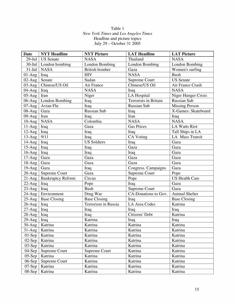
1. Introduction In the 21st century, television brings graphic real-time images of natural and man-made disasters into the homes of millions of Americans, even those who are thousands of miles away from the disaster. It is reasonable to ask whether these images and the accompanying commentary have a significant emotional impact on those watching from a safe distance. In this paper, we use new high-frequency data on subjective feelings collected by the University of Michigan Surveys of Consumers in August, September and October2 of 2005 to examine the emotional reaction of a representative sample of Americans to the news of Hurricane Katrina. Hurricane Katrina struck New Orleans and surrounding areas in late August 2005. A key levy was breached on August 29, 2005, but even the next morning, newspaper headlines did not indicate the seriousness of the eventual situation. For example, on August 30, the New York Times headline was “HURRICANE SLAMS INTO GULF COAST, DOZENS ARE DEAD.” News on the following two days made the seriousness of the disaster clear to those watching the news. On August 31, one day later, the New York Times headline was “NEW ORLEANS IS INUNDATED AS 2 LEVEES FAIL; MUCH OF GULF COAST IS CRIPPLED; DEATH TOLL RISES,” and President Bush gave his first major address on Katrina later that day. Thus, the realization of the seriousness of the damage from hurricane Katrina coincides roughly with the end of August and the beginning of September, 2005. Katrina dominated the news throughout most of September 2005, especially if one considers the coverage of hurricane Rita as part of the same news agenda. (Rita struck the same general area on September 24, and significant coverage of Rita began on September 20 or so.) As an imperfect proxy for this news coverage, Table 1 shows the topics for the top headline and the biggest picture above the fold in the New York Times and the Los Angeles Times from July 29 to October 31.3 From August 30 through September 26, the top headline was about hurricanes Katrina or Rita all but five days in the New York Times and all but five days in the Los Angeles Times. In what is perhaps a better proxy for the TV news coverage, the big picture above the fold in the New York Times was about Katrina or Rita all but six of the 28 days from August 30 through September 26, while the biggest picture above the fold in the Los Angeles Times was about Katrina or Rita all but five days during that period. For comparison, in our entire sample period from July 29 to October 31, the top story in the New York Times was related to Iraq on twenty days and the biggest picture above the fold was related to Iraq on sixteen days. The Los Angeles Times had its top story on Iraq on sixteen days and its big picture on Iraq on eight days. These days were scattered throughout the three month period. Beginning in August 2005, 4 continuing as funding permits, the University of Michigan Surveys of Consumers (the surveys behind the Michigan Consumer Sentiment Index) have

2 One of many sources for a Katrina timeline is www.brookings.edu/fp/projects/ homeland/katrinatimeline.pdf 3 An unpublished appendix available from the authors gives the full headlines for the top two stories and for the story associated with the big picture above the fold for these two papers. 4 “August” 2005 data collection actually began on July 29, 2005, while “October” data collection actually ended on October 24.

3

included the following questions, which are designed to measure the positive or negative dimension of feelings in the previous week:

“Now think about the past week and the feelings you have experienced. Please tell me if each of the following was true for you much of the time this past week:

a. Much of the time during the past week, you felt you were happy. (Would you say yes or no?) b. (Much of the time during the past week,) you felt sad. (Would you say yes or no?) c. (Much of the time during the past week,) you enjoyed life. (Would you say yes or no?) d. (Much of the time during the past week,) you felt depressed. (Would you say yes or no?)”

Approximately 500 respondents were asked these questions in August 2005, and (for budgetary reasons) approximately 300 respondents were asked these questions in each of September and October 2005. This series of questions is the subset focusing on subjective feelings of a widely used Center for Epidemiologic Studies Depression (CES-D) measure of depressive symptoms. Since the answers to these questions can vary widely even within the normal range of feelings, we treat the answers to these four questions as a measure of current happiness or subjective well-being. These are easy questions for respondents to answer: on average the entire series of four questions takes only 36 seconds, or 9 seconds per question. A key advantage of including these questions on the University of Michigan Surveys of Consumers is that the dates of the interviews are spread out throughout most of each month, so that positive and negative feelings in a nationally representative sample of adults can be tracked on a weekly basis. Also, the Surveys of Consumers include information on respondents’ geographic region. Thus, this data are ideal for tracking the week-by-week reaction of current happiness to national or regional news. A key motivation for collecting high frequency data on current happiness is the hypothesis of Kimball and Willis (2006) that a large component of happiness reflects the reaction to recent news about lifetime utility. Here “lifetime utility” represents everything an individual cares about. According to this hypothesis, good news about anything an individual cares about will cause a temporary upward spike in happiness (“elation”). Similarly, bad news about anything the individual cares about will cause a temporary downward spike in happiness (“dismay”). The length of time these spikes in happiness last reflects the time it takes to psychologically process the new information. The magnitude of these spikes reflects the size of the shock to lifetime utility. Thus, according to this hypothesis, spikes in happiness after news give useful information about lifetime utility. A simple partial test of the hypothesis is whether such an interpretation makes sense in actual cases. If the hypothesis passes that test, the next question is the extent to which other hypotheses can also explain the data. In the context of hurricane Katrina, the hypothesis that a large component of happiness reflects the reaction to recent news about lifetime utility predicts that happiness should dip in the first week of September if there was a substantial degree of altruism toward those hurt by the disaster or if people were concerned about the effects of Katrina on government budgets or gasoline prices.5 The outpouring of charitable contributions for Katrina suggests that there was indeed a substantial degree of altruistic concern by many Americans for those hurt by

5 Also, while it is unlikely that the random sample of the survey included many who were directly hurt by Katrina (particularly given the difficulty of reaching those affected on the phone) some of the respondents could have been personally inconvenienced in lesser ways.

4

Katrina. 6 It is less clear how concerned Americans were by the effects of Katrina on their own self-interest. Happiness in later weeks depends on the speed of hedonic adaptation in this context. “Hedonic adaptation” refers to the strong tendency of measured happiness to revert to its previous value after responding to a shock. Frederick and Loewenstein (1999) provide a survey of evidence on hedonic adaptation. Our study provides important evidence about the rate of adaptation in the hedonic effects of national news on onlookers. It is possible that the rate of hedonic adaptation to a shock is a useful indicator of the importance of a shock, along with the magnitude of the initial response of happiness to the shock. If so, the magnitude of the initial response of happiness to Katrina and the speed of hedonic adaptation after that initial response could provide a yardstick for comparison when we observe the happiness of a representative sample of adult Americans responding to events in the future. Alternative hypotheses could explain a negative reaction of happiness to the news of Katrina’s devastation of New Orleans and the surrounding areas. As alluded to above, even within Kimball and Willis’s (2006) hypothesis that news about lifetime utility results in spikes in happiness, Katrina could have generated significant shocks to either the altruistic or the non-altruistic components of the utility function. Stepping away from the hypothesis of happiness responding to news about lifetime utility, it is possible that graphic television images of tragedy in themselves have a big emotional effect. One way to distinguish logically between the effects of news on happiness and the direct effect of the television images is to think of what the likely effect on measured happiness would have been if people had spent an equal amount of time watching a graphic documentary about a disaster of long ago, rather than a real-time disaster. Another possibility is that genuine altruism interacts strongly with graphic images in producing an emotional response—that is, both the graphic images and the fact that they are something happening to real people in the present may be important for the strength of people’s reactions. Unfortunately, we do not have any data on whether these respondents got their news from television or from some other source. As long as the main observed movements in happiness in this time period are, in fact, due to Katrina, any reasonable hypothesis predicts that the happiness of people in the South Central region of the United States (Alabama, Arkansas, Kentucky, Louisiana, Mississippi, Oklahoma, Tennessee, and Texas), which we can identify separately, should dip more than the happiness of people in the remainder of the United States. Altruism is likely to be a function of geographical distance, and those in the region are more likely to know someone, or know someone who knows someone, who was directly affected by the disaster. In terms of self-interest, state budgets in Louisiana and Mississippi were affected by the disaster, and bad news may have been revealed about the quality of state governments as well as the Federal Government. People in those and neighboring states might be inconvenienced by refugees or by difficulty of traveling in the region due to hurricane devastation. As for graphic imagery, television coverage in the region was likely to have been closer to saturation than in the rest of the country, beaming more continuous images of disaster into homes in the South Central region than elsewhere. Nevertheless, to the extent that television coverage of Katrina was close to saturation everywhere in the U.S., a stronger effect in the South Central region could provide some evidence that it was not graphic television imagery alone that drove reactions. 6 According to USA Today, charitable donations to help victims of Katrina and Rita combined are $2.65 billion compared to $2.8 billion for victims of 9/11 and $1.55 billion for the South Asian tsunami (“Katrina inspires record charity,” by Thomas Frank, USA Today, November 14, 2005).

5

2. Results

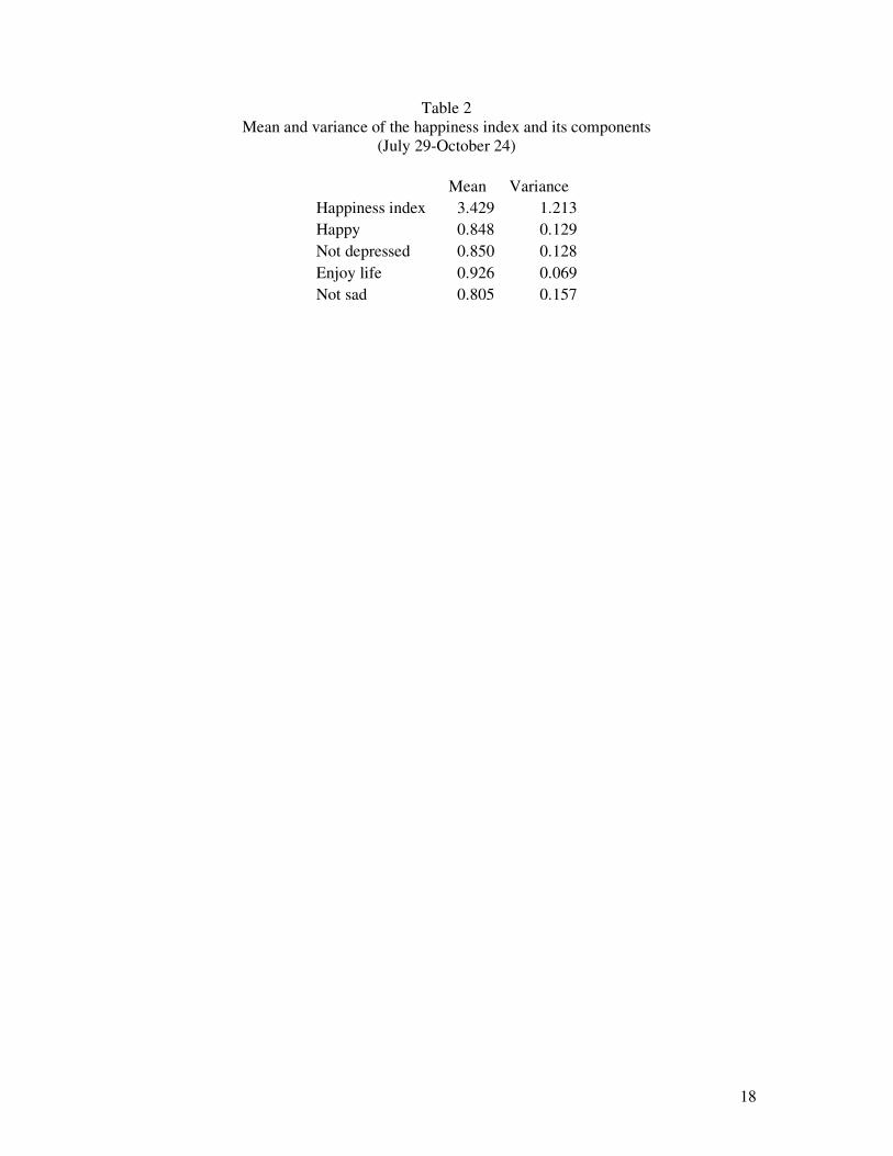
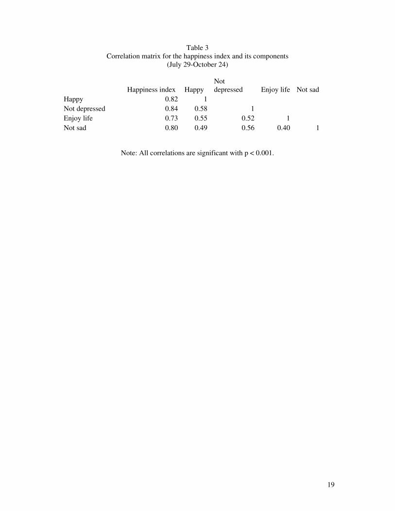
We coded the four yes/no answers into four dichotomous variables, HAPPY, NOT SAD, ENJOY LIFE, NOT DEPRESSED, based on whether the respondent agreed with each of the four questions listed above. The variables NOT SAD and NOT DEPRESSED are reverse coded (e.g. NOT SAD equals one if the respondent said no in response to the statement “Much of the time during the past week, you felt sad.”) For our benchmark results, we construct a happiness index that is the simple sum of these four variables. Table 2 shows the mean and variance of this happiness index and its four components, while Table 3 shows the correlations of these components with each other and of each with the overall happiness index. There is a strong common factor to the four components of the happiness index, which shows up both in the substantial correlations in Table 3 (ranging from .4 to .58 between pairs of components) and in the fact that the overall variance of 1.213 for the happiness index is so far above the sum of the variance of its components. However, it is likely that a large portion of the variance of the happiness index and the correlations among its components is cross-sectional. As discussed by Diener and Lucas (1999), some individuals tend to be chronically happy, while other individuals tend to be chronically unhappy. That variation across individuals is different from the variation over time in the average happiness of a group that is the focus of our analysis. The full sample for August, September and October of 2005 contains 1,528 observations; 1,110 of these were asked the happiness questions and only five of these are missing responses to one or more of the components of our happiness index, so that our sample for analysis has 1,105 observations. Because the Michigan Surveys of Consumers are designed as a monthly survey rather than as a weekly survey, the sample sizes vary from week to week according to the convenience of the interviewing staff and the natural variation in how easy it was to find people at home each week. Sample sizes tend to decline toward the end of each month when the easy-to-catch people have already been interviewed and the interviewers focus on repeatedly contacting the hard-to-catch people. Although these variations in sample size have an important effect on the standard errors we report, we have no reason to think that these routine variations in the sample size from day to day affect our results in any other big way.7 We present many of our results in graphs showing mean values of the happiness index by week. However, these graphs are only suggestive.8 We test the gestalt offered by these 7 To see if this difference between the people interviewed at different points in the month could affect our results, we regressed happiness in August 2005 (which serves as a control, since there was no dramatic news until the very end of the month) on a linear function of the date within the month and found no significant difference between the happiness of those interviewed near the end of the month compared to those interviewed near the beginning of the month. Moreover, in the whole sample, there was no significant effect of the number of contacts necessary to reach a respondent on the reported happiness of that person. The graphs also bear out the absence of a strong, recurring trend in happiness within each month. We also worried about the possibility that Katrina itself could have had a sample selection effect in the South Central region of the United States. The most likely bias is that those with lower socioeconomic status would be especially likely to drop out of the sample because of Katrina, biasing the happiness index in the South Central region upward after Katrina. We return to this issue in the section on results by region (in footnote 18). 8 Our sample size—and therefore our power—is too small to make the graphs anything more than suggestive. In particular, including standard error bands (at the cost of cluttering the graphs) would simply indicate that the statistics for key hypothesis tests are close enough to the critical values for the usual levels of significance to necessitate precise calculations more accurate than one can make visually.

6

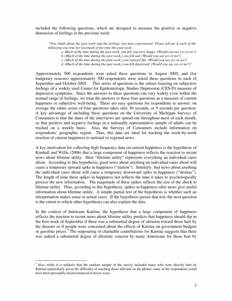
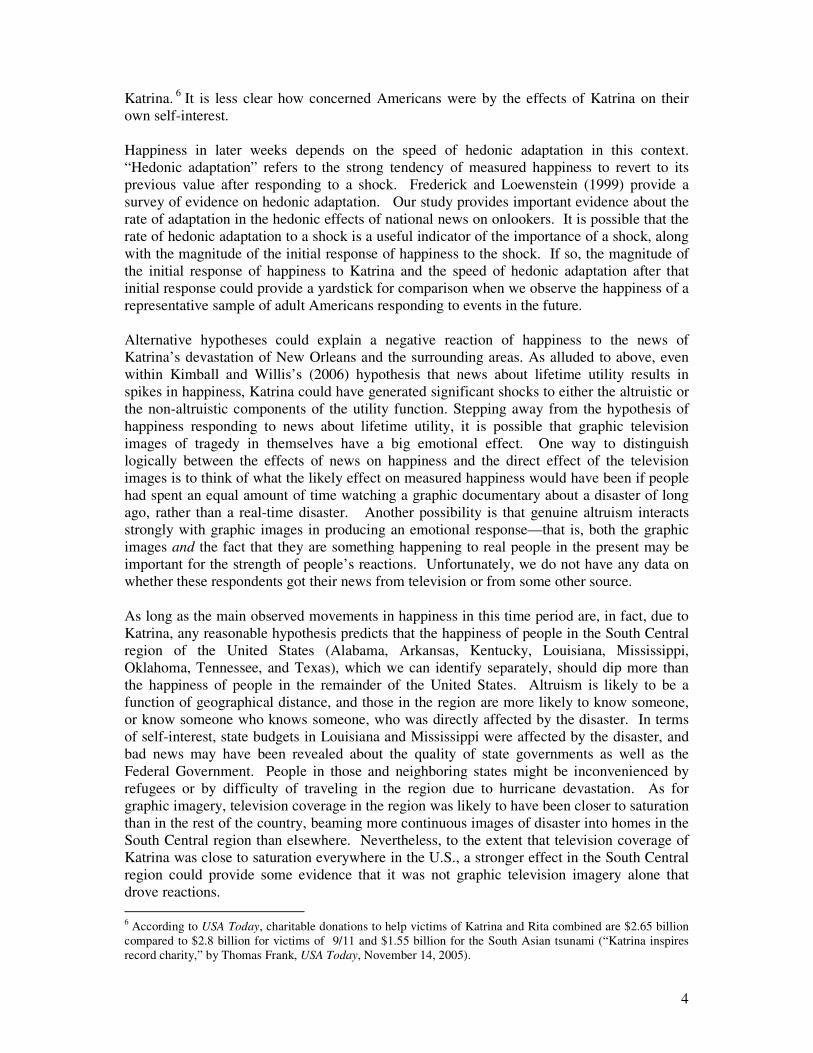
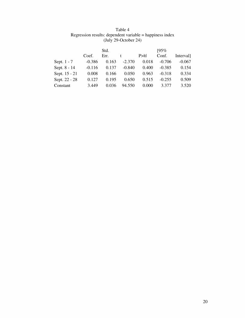
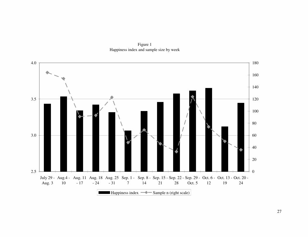
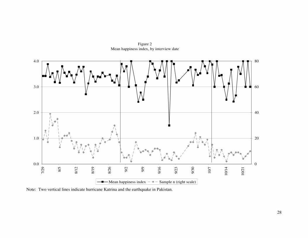
graphs more rigorously with statistical tests to see whether the values for each week in September are significantly different from one another or from the pooled values for August and October. For simplicity and transparency, we use ordinary least squares in our statistical analysis. We consider it unlikely that more sophisticated statistical tools would tell a materially different story. We will call a difference “not statistically significant” if there is more than a 10% chance that it could arise by chance as a result of sampling error using a two-tailed test, and report the probability itself for notable differences that have less than a 10% chance of arising by chance. In most cases, the statistical analysis supports the story told by the picture. Main results. Figure 1 shows the average value of the happiness index and the sample size in each week. The weeks are defined as Thursday to Wednesday so that the seven days from September 1 to September 7 are represented by one bar.9 Figure 1 shows the predicted dip in the happiness index in the first week of September. To verify that this dip is not due to sampling error, Table 4 reports an OLS regression of the weekly happiness index on a constant and dummy variables for September 1-7, September 8-14, September 15-21 and September 22-28; the baseline period for comparison is all observations from July 29 through August 31 or from September 29 through October 24, or approximately all of August and October pooled.10 There is only a 1.8% probability that the average happiness index in the first week of September would be this much lower than the average value for all of August and October by chance. The other dramatic aspect of Figure 1 is the return of the happiness index to normal by late September. In terms of the average value of the happiness index, neither September 8-14 nor September 15-21 is significantly different from the baseline in August and October. Moreover, the probability that the average value of the happiness index would be this much higher in September 15-21 as compared to September 1-7 by chance is only 8.3%. Thus, it appears that more-or-less full hedonic adaptation to the news about Katrina took place within a few weeks’ time after the initial news. Figure 2 graphs the average happiness index day by day, to show that our particular grouping of days into weeks does not drive the results. The line at the bottom shows the daily sample size, which explains why, with sampling error, the average happiness index bounces around from day to day as much as it does. Though there is not enough data to be certain, this day-by-day picture of the data suggests some delay beyond the beginning of September 1 in the dip in happiness. One important reason for this could be the wording of the questions, which ask for people’s feelings during “much of the last week.” For those respondents who took this reference to “much of the last week” seriously, considerable unhappiness for the past day or two might not qualify as unhappiness “much of the last week.” Once several days have passed since the full gravity and emotional import of Katrina have sunk in, there is no ambiguity about how to respond to the question.11 A more subtle reason for the delay in the reaction of measured happiness, in line with research on subjective well-being reports 9 98.8% of the phone interviews are completed within a single day, making the day of interview unambiguous. For the remaining 1.2% of respondents, we use the day the interview ended, since the data behind the happiness index is collected near the end of the survey. 10 It is evident in figure 1 that there is another large dip in the happiness index in the week October 13-19. Below, we discuss the possibility that this dip is due to the earthquake that shook Pakistan on October 8. (See for example, http://www.mercurynews.com/mld/mercurynews/news/world/12868152.htm) For now we pool all of the August and October data in order to focus on the effects of Katrina. 11 Given that our sample size makes it difficult to identify significant day-to-day fluctuations in happiness, we consider this wording appropriate.

7

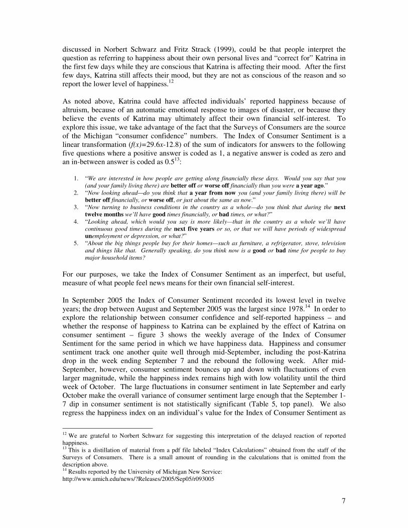
discussed in Norbert Schwarz and Fritz Strack (1999), could be that people interpret the question as referring to happiness about their own personal lives and “correct for” Katrina in the first few days while they are conscious that Katrina is affecting their mood. After the first few days, Katrina still affects their mood, but they are not as conscious of the reason and so report the lower level of happiness.12 As noted above, Katrina could have affected individuals’ reported happiness because of altruism, because of an automatic emotional response to images of disaster, or because they believe the events of Katrina may ultimately affect their own financial self-interest. To explore this issue, we take advantage of the fact that the Surveys of Consumers are the source of the Michigan “consumer confidence” numbers. The Index of Consumer Sentiment is a linear transformation (f(x)=29.6x-12.8) of the sum of indicators for answers to the following five questions where a positive answer is coded as 1, a negative answer is coded as zero and an in-between answer is coded as 0.513:

1. “We are interested in how people are getting along financially these days. Would you say that you (and your family living there) are better off or worse off financially than you were a year ago.”

2. “Now looking ahead—do you think that a year from now you (and your family living there) will be better off financially, or worse off, or just about the same as now.”

3. “Now turning to business conditions in the country as a whole—do you think that during the next twelve months we’ll have good times financially, or bad times, or what?”

4. “Looking ahead, which would you say is more likely—that in the country as a whole we’ll have continuous good times during the next five years or so, or that we will have periods of widespread unemployment or depression, or what?”

5. “About the big things people buy for their homes—such as furniture, a refrigerator, stove, television and things like that. Generally speaking, do you think now is a good or bad time for people to buy major household items?

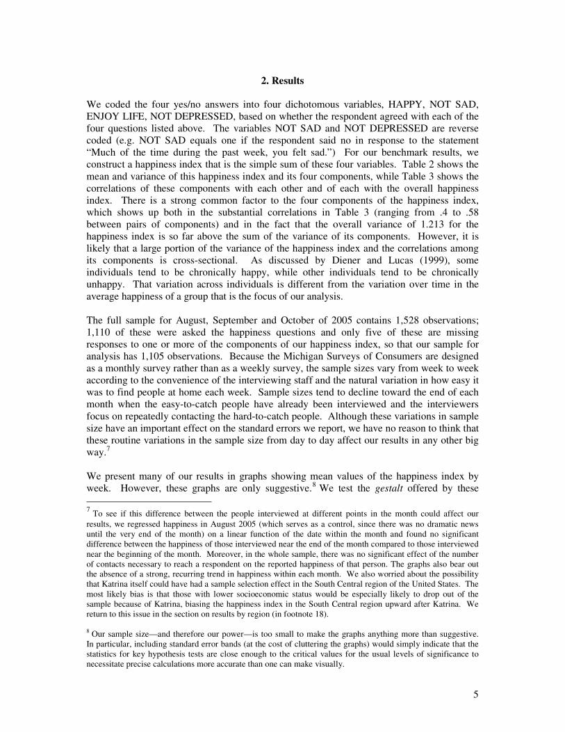
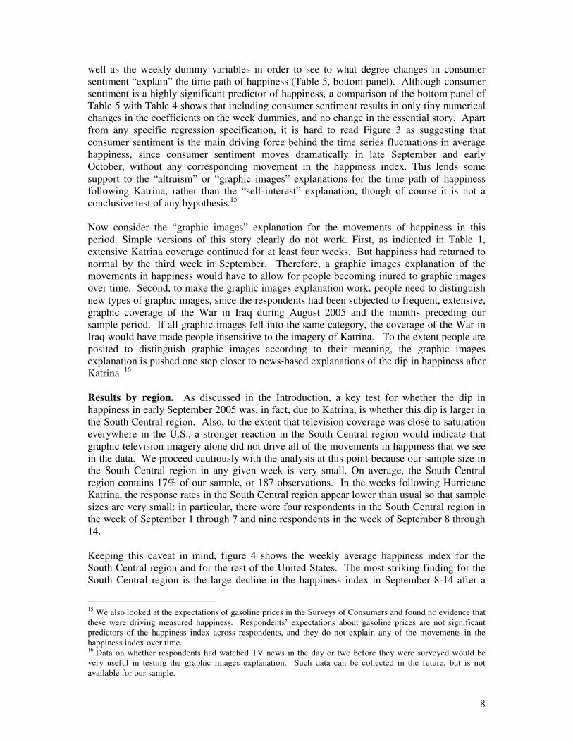
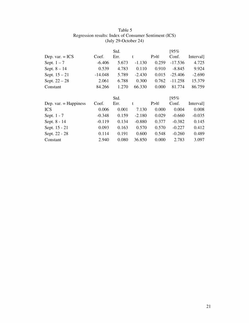
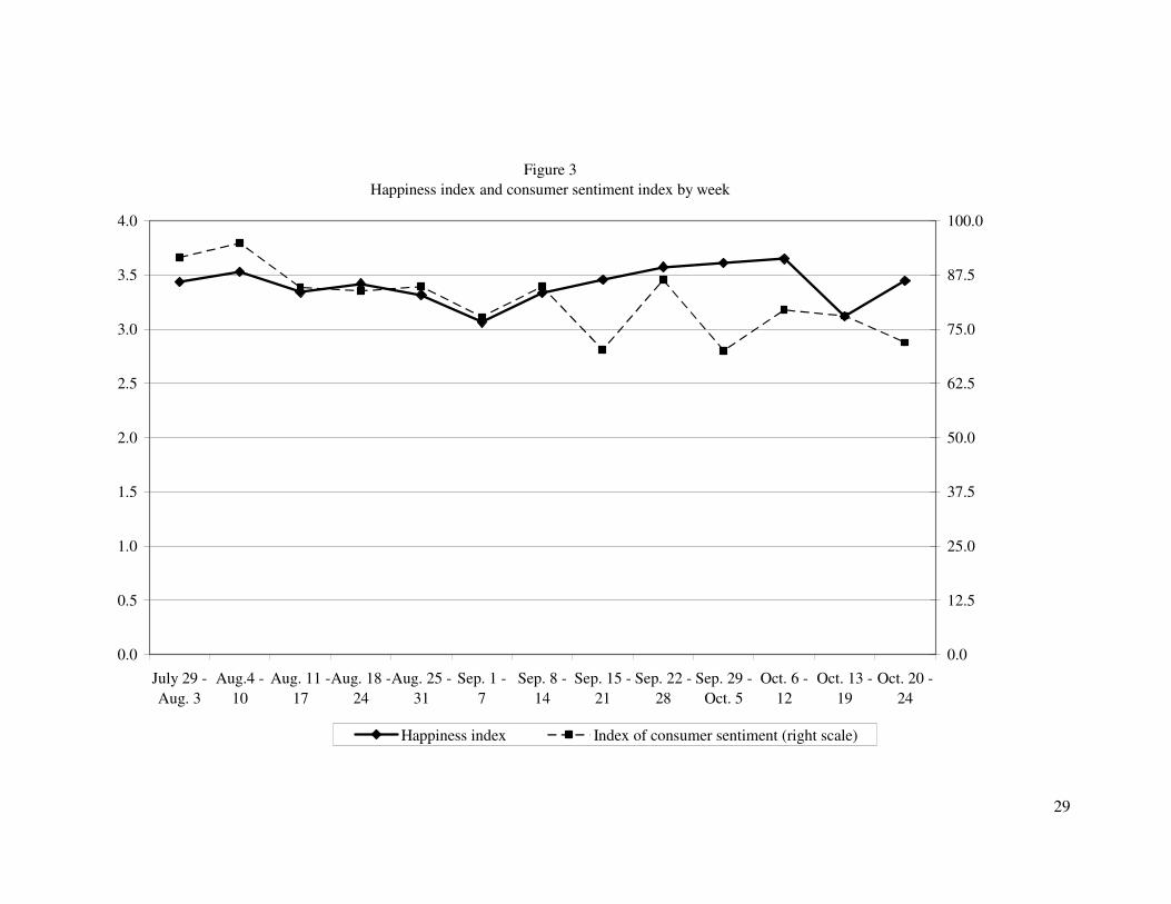
For our purposes, we take the Index of Consumer Sentiment as an imperfect, but useful, measure of what people feel news means for their own financial self-interest. In September 2005 the Index of Consumer Sentiment recorded its lowest level in twelve years; the drop between August and September 2005 was the largest since 1978.14 In order to explore the relationship between consumer confidence and self-reported happiness – and whether the response of happiness to Katrina can be explained by the effect of Katrina on consumer sentiment – figure 3 shows the weekly average of the Index of Consumer Sentiment for the same period in which we have happiness data. Happiness and consumer sentiment track one another quite well through mid-September, including the post-Katrina drop in the week ending September 7 and the rebound the following week. After mid-September, however, consumer sentiment bounces up and down with fluctuations of even larger magnitude, while the happiness index remains high with low volatility until the third week of October. The large fluctuations in consumer sentiment in late September and early October make the overall variance of consumer sentiment large enough that the September 1-7 dip in consumer sentiment is not statistically significant (Table 5, top panel). We also regress the happiness index on an individual’s value for the Index of Consumer Sentiment as

12 We are grateful to Norbert Schwarz for suggesting this interpretation of the delayed reaction of reported happiness. 13 This is a distillation of material from a pdf file labeled “Index Calculations” obtained from the staff of the Surveys of Consumers. There is a small amount of rounding in the calculations that is omitted from the description above. 14 Results reported by the University of Michigan New Service: http://www.umich.edu/news/?Releases/2005/Sep05/r093005

8

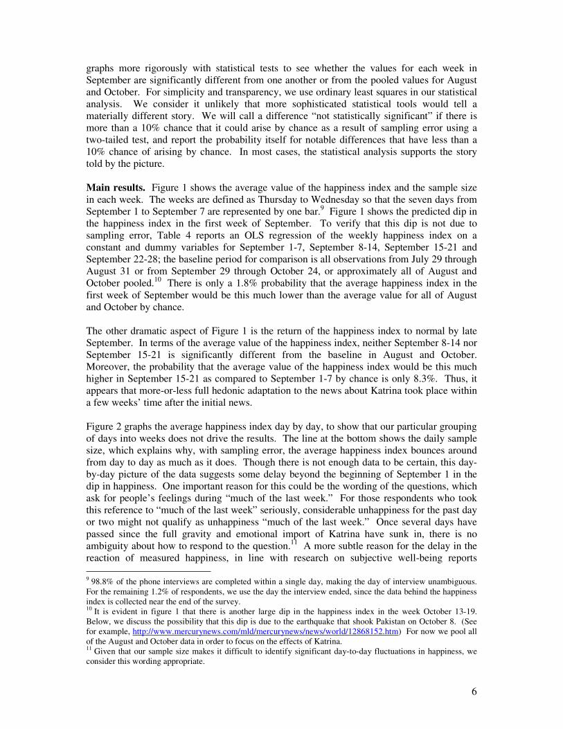
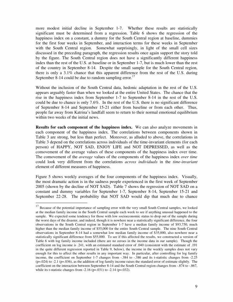
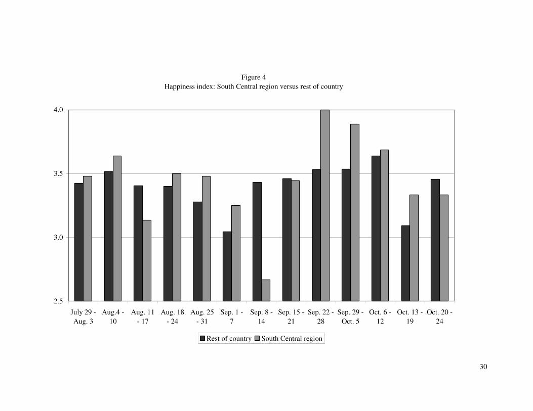
well as the weekly dummy variables in order to see to what degree changes in consumer sentiment “explain” the time path of happiness (Table 5, bottom panel). Although consumer sentiment is a highly significant predictor of happiness, a comparison of the bottom panel of Table 5 with Table 4 shows that including consumer sentiment results in only tiny numerical changes in the coefficients on the week dummies, and no change in the essential story. Apart from any specific regression specification, it is hard to read Figure 3 as suggesting that consumer sentiment is the main driving force behind the time series fluctuations in average happiness, since consumer sentiment moves dramatically in late September and early October, without any corresponding movement in the happiness index. This lends some support to the “altruism” or “graphic images” explanations for the time path of happiness following Katrina, rather than the “self-interest” explanation, though of course it is not a conclusive test of any hypothesis.15 Now consider the “graphic images” explanation for the movements of happiness in this period. Simple versions of this story clearly do not work. First, as indicated in Table 1, extensive Katrina coverage continued for at least four weeks. But happiness had returned to normal by the third week in September. Therefore, a graphic images explanation of the movements in happiness would have to allow for people becoming inured to graphic images over time. Second, to make the graphic images explanation work, people need to distinguish new types of graphic images, since the respondents had been subjected to frequent, extensive, graphic coverage of the War in Iraq during August 2005 and the months preceding our sample period. If all graphic images fell into the same category, the coverage of the War in Iraq would have made people insensitive to the imagery of Katrina. To the extent people are posited to distinguish graphic images according to their meaning, the graphic images explanation is pushed one step closer to news-based explanations of the dip in happiness after Katrina. 16 Results by region. As discussed in the Introduction, a key test for whether the dip in happiness in early September 2005 was, in fact, due to Katrina, is whether this dip is larger in the South Central region. Also, to the extent that television coverage was close to saturation everywhere in the U.S., a stronger reaction in the South Central region would indicate that graphic television imagery alone did not drive all of the movements in happiness that we see in the data. We proceed cautiously with the analysis at this point because our sample size in the South Central region in any given week is very small. On average, the South Central region contains 17% of our sample, or 187 observations. In the weeks following Hurricane Katrina, the response rates in the South Central region appear lower than usual so that sample sizes are very small: in particular, there were four respondents in the South Central region in the week of September 1 through 7 and nine respondents in the week of September 8 through 14. Keeping this caveat in mind, figure 4 shows the weekly average happiness index for the South Central region and for the rest of the United States. The most striking finding for the South Central region is the large decline in the happiness index in September 8-14 after a

15 We also looked at the expectations of gasoline prices in the Surveys of Consumers and found no evidence that these were driving measured happiness. Respondents’ expectations about gasoline prices are not significant predictors of the happiness index across respondents, and they do not explain any of the movements in the happiness index over time. 16 Data on whether respondents had watched TV news in the day or two before they were surveyed would be very useful in testing the graphic images explanation. Such data can be collected in the future, but is not available for our sample.

9

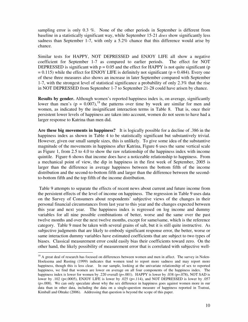
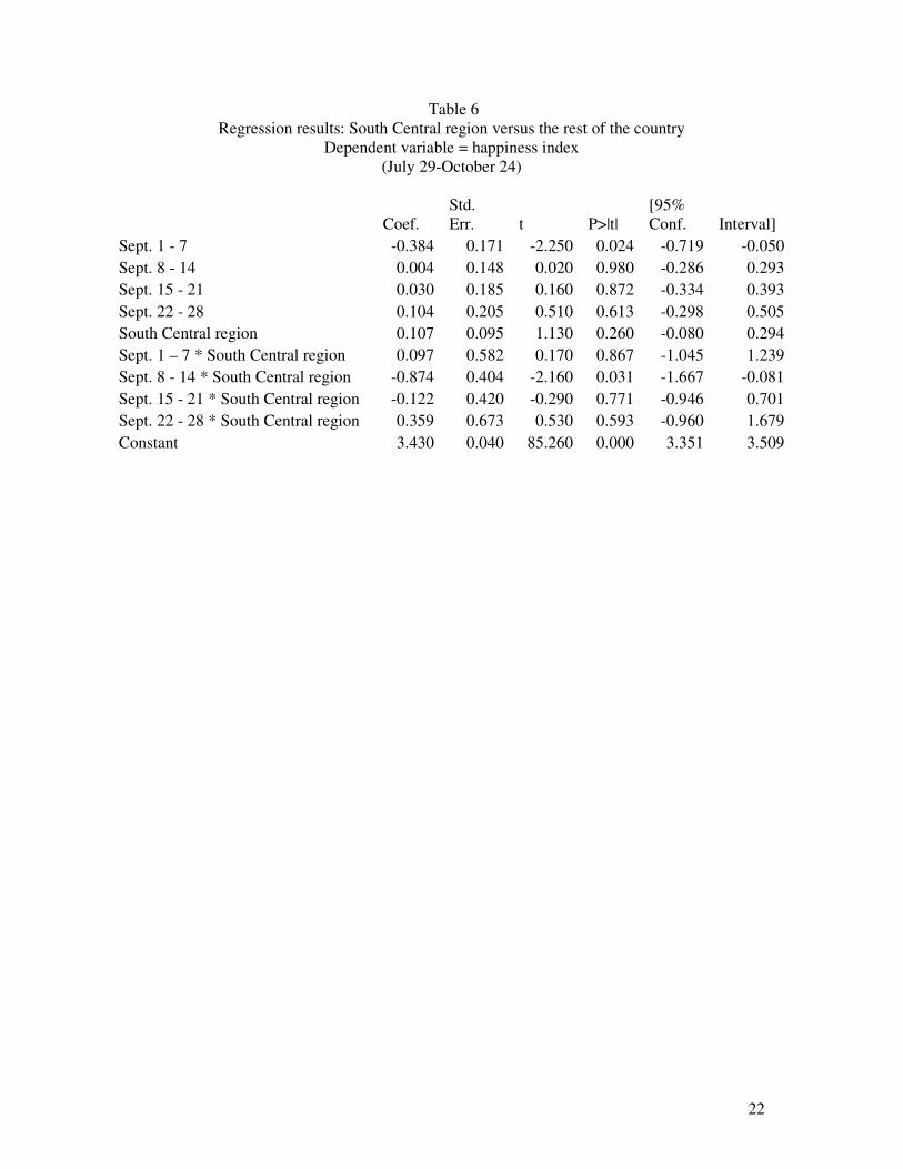
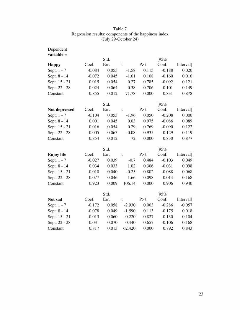
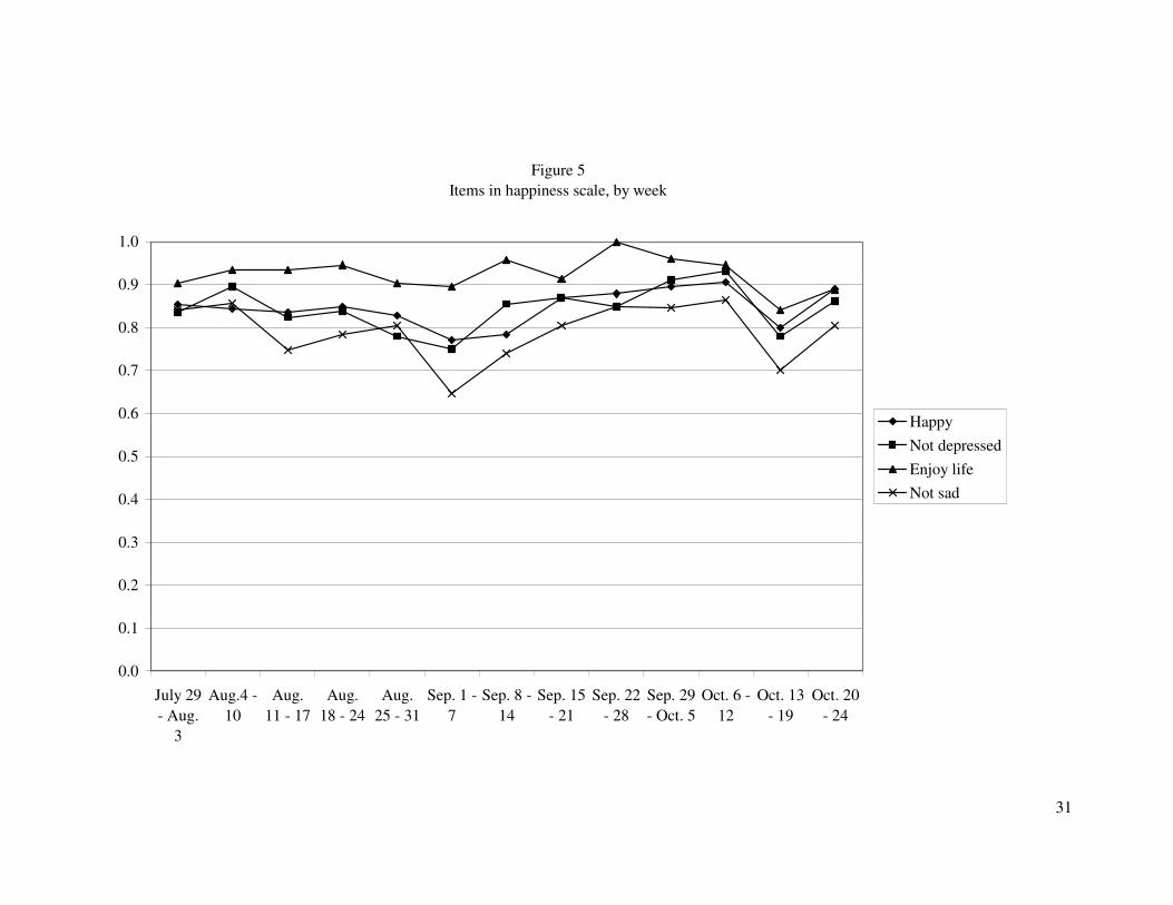
more modest initial decline in September 1-7. Whether these results are statistically significant must be determined from a regression. Table 6 shows the regression of the happiness index on a constant, a dummy for the South Central region at baseline, dummies for the first four weeks in September, and interaction terms for these weeks in September with the South Central region. Somewhat surprisingly, in light of the small cell sizes discussed in the preceding paragraph, the regression results once again support the story told by the figure. The South Central region does not have a significantly different happiness index than the rest of the U.S. at baseline or in September 1-7, but is much lower than the rest of the country in September 8-14. Despite the small sample for the South Central region, there is only a 3.1% chance that this apparent difference from the rest of the U.S. during September 8-14 could be due to random sampling error.17 Without the inclusion of the South Central data, hedonic adaptation in the rest of the U.S. appears arguably faster than when we looked at the entire United States. The chance that the rise in the happiness index from September 1-7 to September 8-14 in the rest of the U.S. could be due to chance is only 7.6%. In the rest of the U.S. there is no significant difference of September 8-14 and September 15-21 either from baseline or from each other. Thus, people far away from Katrina’s landfall seem to return to their normal emotional equilibrium within two weeks of the initial news. Results for each component of the happiness index. We can also analyze movements in each component of the happiness index. The correlations between components shown in Table 3 are strong, but less than perfect. Moreover, as alluded to above, the correlations in Table 3 depend on the correlations across individuals of the time-invariant elements (for each person) of HAPPY, NOT SAD, ENJOY LIFE and NOT DEPRESSED, as well as the comovement of the average values of these components of the happiness index over time. The comovement of the average values of the components of the happiness index over time could look very different from the correlations across individuals in the time-invariant element of different measures of happiness. Figure 5 shows weekly averages of the four components of the happiness index. Visually, the most dramatic action is in the sadness people experienced in the first week of September 2005 (shown by the decline of NOT SAD). Table 7 shows the regression of NOT SAD on a constant and dummy variables for September 1-7, September 8-14, September 15-21 and September 22-28. The probability that NOT SAD would dip that much due to chance 17 Because of the potential importance of sampling error with the very small South Central samples, we looked at the median family income in the South Central sample each week to see if anything unusual happened to the sample. We expected some tendency for those with low socioeconomic status to drop out of the sample during the worst days of the disaster, and indeed, though it is nowhere near a statistically significant difference, the four observations in the South Central region in September 1-7 have a median family income of $93,750, much higher than the median family income of $55,000 for the entire South Central sample. The nine South Central observations in September 8-14 had a somewhat low median family income of $35,000, also nowhere near a statistically significant difference from $55,000. To see if this affected the results, we constructed a version of Table 6 with log family income included (there are no zeroes in the income data in our sample). Though the coefficient on log income is .241, with an estimated standard error of .040 (consistent with the estimate of .191 in the quite different regression reported in Table 9, below), the income in the weekly samples does not vary enough for this to affect the other results in any important way. In particular, after controlling for log family income, the coefficient on September 1-7 changes from -.384 to -.386 and its t-statistic changes from -2.25 (p=.024) to -2.1 (p=.036), as the addition of log family income raises the standard error of estimate slightly. The coefficient on the interaction between September 8-14 and the South Central region changes from -.874 to -.867, while its t-statistic changes from -2.16 (p=.031) to -2.14 (p=.032).

10

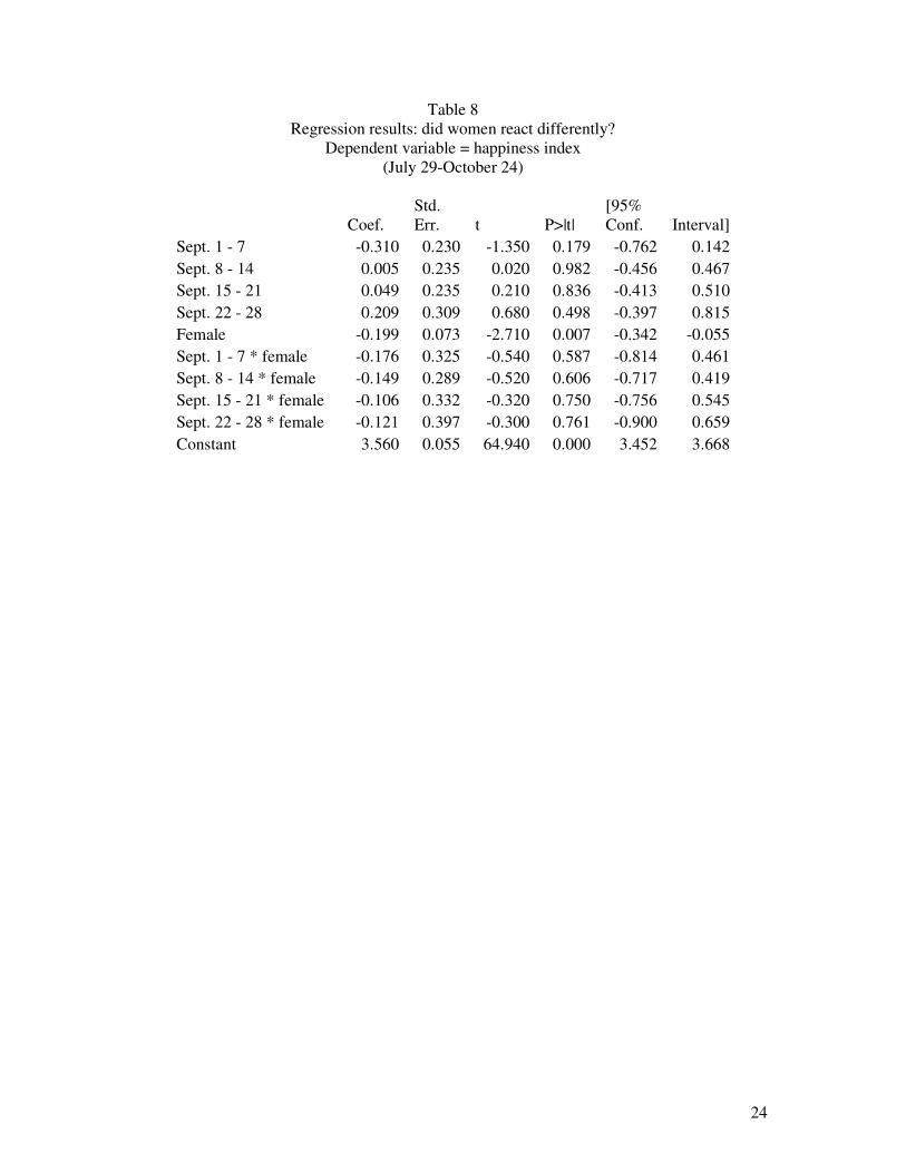
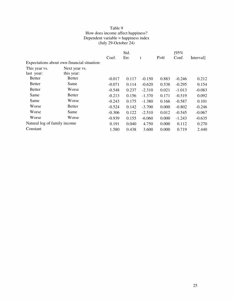
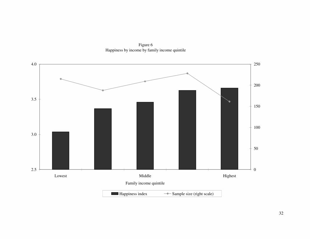
sampling error is only 0.3 %. None of the other periods in September is different from baseline in a statistically significant way, while September 15-21 does show significantly less sadness than September 1-7, with only a 5.2% chance that this difference would arise by chance. Similar tests for HAPPY, NOT DEPRESSED and ENJOY LIFE all show a negative coefficient for September 1-7 as compared to earlier periods. The effect for NOT DEPRESSED is significant with p = 0.05 and the effect for HAPPY is not quite significant (p = 0.115) while the effect for ENJOY LIFE is definitely not significant (p = 0.484). Every one of these three measures also shows an increase in later September compared with September 1-7, with the strongest level of statistical significance a probability of only 2.3% that the rise in NOT DEPRESSED from September 1-7 to September 21-28 could have arisen by chance. Results by gender. Although women’s reported happiness index is, on average, significantly lower than men’s (p = 0.007),18 the patterns over time by week are similar for men and women, as indicated by the insignificant interaction terms in Table 8. That is, once their persistent lower levels of happiness are taken into account, women do not seem to have had a larger response to Katrina than men did. Are these big movements in happiness? It is logically possible for a decline of .386 in the happiness index as shown in Table 4 to be statistically significant but substantively trivial. However, given our small sample sizes, this is unlikely. To give some idea of the substantive magnitude of the movements in happiness after Katrina, Figure 6 uses the same vertical scale as Figure 1, from 2.5 to 4.0 to show the raw relationship of the happiness index with income quintile. Figure 6 shows that income does have a noticeable relationship to happiness. From a mechanical point of view, the dip in happiness in the first week of September, 2005 is larger than the difference in average happiness between the bottom fifth of the income distribution and the second-to-bottom fifth and larger than the difference between the second-to-bottom fifth and the top fifth of the income distribution. Table 9 attempts to separate the effects of recent news about current and future income from the persistent effects of the level of income on happiness. The regression in Table 9 uses data on the Survey of Consumers about respondents’ subjective views of the changes in their personal financial circumstances from last year to this year and the changes expected between this year and next year. The happiness index is regressed on log income and dummy variables for all nine possible combinations of better, worse and the same over the past twelve months and over the next twelve months, except for same/same, which is the reference category. Table 9 must be taken with several grains of salt, but it is still quite instructive. As subjective judgments that are likely to embody significant response error, the better, worse or same interaction dummy variables have estimated coefficients that are subject to two types of biases. Classical measurement error could easily bias their coefficients toward zero. On the other hand, the likely possibility of measurement error that is correlated with subjective well- 18 A great deal of research has focused on differences between women and men in affect. The survey in Nolen-Hoeksema and Rusting (1999) indicates that women tend to report more sadness and may report more happiness, though this is less clear. In our sample, looking at the univariate relationship of sex to reported happiness, we find that women are lower on average on all four components of the happiness index. The happiness index is lower for women by .220 overall (p=.001). HAPPY is lower by .038 (p=.078), NOT SAD is lower by .102 (p<.0005), ENJOY LIFE is lower by .025 (p=.114), and NOT DEPRESSED is lower by .057 (p=.008). We can only speculate about why the sex difference in happiness goes against women more in our data than in other data, including the data on a single-question measure of happiness reported in Tsutsui, Kimball and Ohtake (2006). Addressing that question is beyond the scope of this paper.

11

being could generate coefficients like those in the table even with no genuine relationship.19 Nevertheless, the estimates in Table 9 do give some idea of the order of magnitude of various effects, suggesting that .386 is not a trivial change in the happiness index. Table 9 is instructive in another way. Imagine for just this one paragraph that the econometric issues surrounding Table 9 were solved by a miraculous absence of measurement error in the subjective measures of change in financial circumstances. It would still be important to caution that the size of the dip in happiness shown in Table 4 cannot be directly compared to any of the numbers in Table 9. Kimball and Willis (2006) argue that persistent, predictable effects on happiness are different in character from the response of happiness to news. The effect of income that remains in Table 9 after controlling, to some extent, for recent and expected future changes in financial situation arguably contains a strong component of such a persistent, predictable effect of income on happiness. The effects of changes and expected future changes in financial circumstances on happiness are more closely related to the effect of news on happiness, but the news associated with those changes in financial circumstances could have come a long time ago. For example, some of the news relevant to changes in financial circumstances last year may be several years old, with the events in the last year no surprise at all. Even if the change in the last year was a surprise, on average, most respondents will have had months to get used to many of the key pieces of news about their financial circumstances. By contrast, we are looking at the effects of Katrina on happiness in the first few weeks after the event. According to Kimball and Willis’s (2006) theory, it would be legitimate to compare the dip in happiness after Katrina to the effects of receiving news about income if we collected happiness data in the weeks immediately before and after respondents received notification of salary or wage increases (or decreases), and collected expectations data to isolate the part of the wage increase that was a surprise. However, even with news about personal finances being older news than news about Katrina, if the estimates in Table 9 were consistent, they would allow one to say something about the size of the typical blow to one’s expected utility in the bad case when one finds out that one’s financial circumstances this year will be worse than last year. To wit, given the length of time the average respondent will have had to get used to news about the last twelve month’s changes in personal financial circumstances by the time they show up in our data set, our data suggest that on impact, negative news about one’s personal financial circumstances tends to represent a much heavier blow than the blow one suffers from seeing that people in New Orleans and surrounding areas are suffering. After months on average to get used to negative personal financial news during the last year, the coefficients of -.524, -.306 and -.939, taken at face value, are much more negative than the undetectable effect of Katrina on the happiness of onlookers after a month or two and almost as large or larger than the effect of Katrina on happiness after one week. This would be as one should expect. In casual observation, we see evidence that many people care about others, but few are saints. The foregoing discussion helps to clarify where our statistical identification comes from in our main results. Subjective well-being is, of course, measured with error, but error in a dependent variable does not by itself bias estimates. The independent variables in our main results are objective regional, national and world events or non-events, in some cases interacted with objective respondent characteristics. In the case of Katrina, it is reasonably clear that only a small fraction of the eventual catastrophe was expected in advance to result from this particular hurricane. To the extent that the harm from Katrina was expected, this biases the estimated coefficients toward zero.

19 Hamermesh (2004) points out that this is a general danger when regressing one subjective variable on another.

12

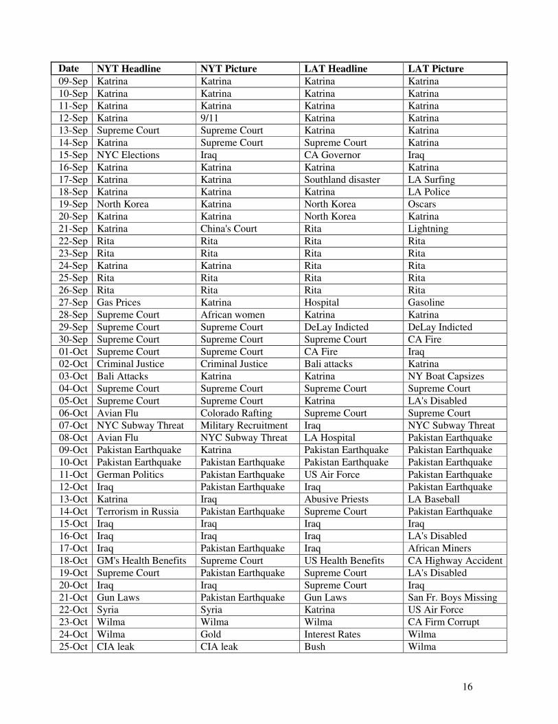
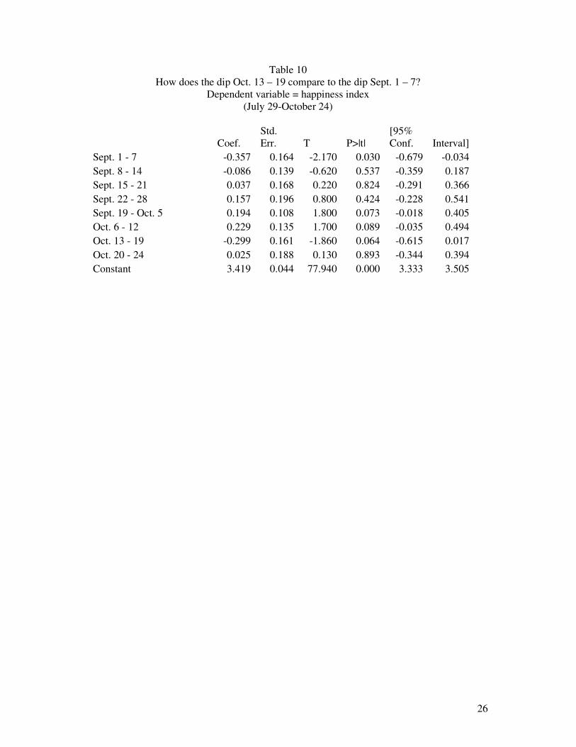
3. Did American Happiness React to the Earthquake in Pakistan? A major earthquake hit Pakistan and neighboring areas of India on October 8, 2005. The ultimate death toll exceeded 79,000.20 The top headline in both the New York Times and the Los Angeles Times was about this earthquake on October 9 and October 10. In what we have argued is a better proxy for the TV news coverage, the biggest picture above the fold in the New York Times was about the earthquake in Pakistan and its aftermath on the seven days October 10-12,14,17,19 and 21. The Los Angeles Times big picture was about the earthquake in Pakistan on the six days October 8-12 and 14. Overall, the earthquake in Pakistan was a major story. As can be seen from Table 1, in our period of analysis, only Katrina, Rita and the War in Iraq surpassed the earthquake in Pakistan in this measure of pictorial coverage.21 Because events in Iraq were spread throughout our period of analysis, with no sudden change in the situation there, they are not good candidates for causing a spike or dip in happiness visible within this period. Rita was probably seen by many as a continuation of the tragedy of Katrina and did not ultimately worsen the damage very much. Thus, other than Katrina, the earthquake in Pakistan is arguably the best place to look for detectable effects on happiness. As noted earlier, Figure 1 does show a dip in happiness in the week of October 13-19, following the earthquake in Pakistan.22 Table 10 shows that the October 13-19 dip had only a 6.4% probability of occurring by chance. Although the point estimate is somewhat smaller in absolute value, there is no statistically significant difference between the size of the dip in September 1-7 and the dip in October 13-19. The relatively high coefficient on October 6-12 is somewhat contrary, but the day by day graph in Figure 2 shows that October 6, 7 and 8 (before some respondents had heard of the earthquake in Pakistan) had relatively happy respondents and substantial sample sizes. Overall, Figure 2 shows a reaction to the earthquake (if it was a reaction to the earthquake) that was delayed in relation to the beginning of the tragedy in a way not dramatically dissimilar to the reaction to Katrina. In addition to the wording of the questions, which ask about how the respondent felt “much of the time during the past week,” and the possible “correction” people make for the influence of an event on their happiness while they are conscious of the effect, some of this delay might reflect the time it took TV news agencies to gear up for full-scale coverage, especially when the story was in a remote area on the other side of the world. The response of happiness to future events will provide further evidence on whether such a delay in the reaction of reported happiness to events is common. Taking

20See http://www.boston.com/news/world/asia/articles/2005/10/20/pakistan_earthquake_death_toll_rises_to_79000/ 21 During our sample period, the big picture above the fold was about U.S. Supreme Court nominations ten days in the New York Times and three days in the Los Angeles Times, which ties the total of thirteen days in the two papers for the earthquake in Pakistan. Pictures about the Supreme Court nominations were less concentrated in time than pictures about the earthquake in Pakistan. Also, unlike the coverage of the earthquake in Pakistan—which should represent bad news to almost everyone—news about Supreme Court nominations should represent bad news to some respondents and good news to others, depending on each respondent’s politics. We do not have information on political leanings in this U.S. data set, but the companion paper Tsutsui, Kimball and Ohtake (2006) examines how the politics of individuals in Japan affects the time series of responses to news about Prime Minister Koizumi’s victory in Japanese elections held on September 11, 2005. 22 We do not have enough data for statistical significance after dividing the sample, but according to point estimates, the happiness index dipped in this week in all four major regions: West, Midwest, Northeast and South. This is consistent with the idea that the cause was an international event.

13

stock, there is some evidence of a dip in happiness related to the earthquake in Pakistan, but the level of statistical significance is not as high as for the dip in happiness due to Katrina. If the dip in happiness after Katrina was due to altruistic concern, and the dip in happiness in October 13-19 was caused by the earthquake in Pakistan, as we suspect, this reaction of happiness could be viewed as an indication of how much altruism Americans feel toward people on the other side of the world. The larger death toll from this earthquake than from Katrina makes it more likely that Americans would not just brush it off if they did feel substantial concern. Alternatively, it is logically possible that the graphic images of suffering generated by the earthquake in Pakistan could have caused a dip in happiness by some more direct psychological mechanism not mediated by caring, assuming the graphic images of suffering in Pakistan were experienced as distinct from the graphic images related to Katrina and the war in Iraq.23

4. Conclusion Our results suggest that Hurricane Katrina significantly reduced the reported happiness of a nationally representative sample of adults in the US. These effects were even larger for the subsample in the South Central region closest to Katrina. The effects of Katrina were similar for men and for women. We find that happiness is correlated with, but distinct from consumer sentiment, calling into question an explanation of these movements in happiness based only on self-interest. Rather, we believe that altruism or a more general emotional response to images of new disasters is likely to explain this response to bad news. We also find that individuals adapt rather quickly to bad news about world events: reported happiness had returned to normal in the rest of the country within two weeks after the disaster and within three weeks after the disaster in the South Central region. We view this study as an example of a method that can be applied more generally to study what kinds of events strike the average respondent as noteworthy good news or noteworthy bad news. For example, the strong hint of a response of happiness to the earthquake in Pakistan in October provides some evidence relevant to the question of how concerned Americans were about the Pakistanis affected by that tragedy.

23 Although not impossible, it seems unlikely to us that average American happiness reacted to the earthquake in Pakistan out of self-interest.

14

References Diener, Ed and Richard E. Lucas, 1999. “Personality and Subjective Well-Being,” chapter 11 in Daniel Kahneman, Ed Diener and Norbert Schwarz eds., Well-Being: The Foundations of Hedonic Psychology, Russell Sage Foundation, New York. Frederick, Shane, and George Loewenstein, 1999. “Hedonic Adaptation,” chapter 16 in Daniel Kahneman, Ed Diener and Norbert Schwarz eds., Well-Being: The Foundations of Hedonic Psychology, Russell Sage Foundation, New York. Hamermesh, Daniel S., 2004. “Subjective Outcomes in Economics,” Southern Economic Journal (July). Kimball, Miles and Robert Willis, 2006. “Utility and Happiness,” University of Michigan. Nolen-Hoeksema and Cheryl L. Rusting, 1999. “Gender Differences in Well-Being” chapter 17 in Daniel Kahneman, Ed Diener and Norbert Schwarz eds., Well-Being: The Foundations of Hedonic Psychology, Russell Sage Foundation, New York. Schwarz, Norbert and Fritz Strack, 1999. “Reports of Subjective Well-Being: Judgmental Processes and Their Methodological Implications,” chapter 4 in Daniel Kahneman, Ed Diener and Norbert Schwarz eds., Well-Being: The Foundations of Hedonic Psychology, Russell Sage Foundation, New York. Tsutsui, Yoshiro, Miles Kimball and Fumio Ohtake, 2006. “Koizumi Carried the Day: Did the Japanese Election Results Make People Happy and Unhappy?” Osaka University and University of Michigan.

15

Table 1 New York Times and Los Angeles Times

Headline and picture topics July 29 – October 31 2005

Date NYT Headline NYT Picture LAT Headline LAT Picture

29-Jul US Senate NASA Thailand NASA 30-Jul London bombing London Bombing London Bombing London Bombing 31-Jul NASA British bomber Gaza Women's surfing

01-Aug Iraq HIV NASA Bush 02-Aug Senate Sudan Supreme Court US Senate 03-Aug Chinese/US Oil Air France Chinese/US Oil Air France Crash 04-Aug Iraq NASA Iraq NASA 05-Aug Iran Niger LA Hospital Niger Hunger Crisis 06-Aug London Bombing Iraq Terrorists in Britain Russian Sub 07-Aug Avian Flu Iraq Russian Sub Missing Person 08-Aug Gaza Russian Sub Iraq X-Games: Skateboard 09-Aug Iran Iraq Iran Iraq 10-Aug NASA Colombia NASA NASA 11-Aug Iraq Gaza Gas Prices LA Watts Riot 12-Aug Iraq Iraq Iraq Tall Ships in LA 13-Aug 9/11 Iraq CA Voting LA Mass Transit 14-Aug Iraq US Soldiers Iraq Gaza 15-Aug Iraq Iraq Gaza Gaza 16-Aug Iraq Iraq Iraq Gaza 17-Aug Gaza Gaza Gaza Gaza 18-Aug Gaza Gaza Gaza Gaza 19-Aug Gaza Iraq Congress. Campaigns Gaza 20-Aug Supreme Court Gaza Supreme Court Pope 21-Aug Bankruptcy Reform Circus Pope US Health Care 22-Aug Iraq Pope Iraq Gaza 23-Aug Iraq Bush Supreme Court Gaza 24-Aug Environment Drug War CA-Donations to Gov. Animal Shelter 25-Aug Base Closing Base Closing Iraq Base Closing 26-Aug Iraq Terrorism in Russia LA Area Codes Katrina 27-Aug Iraq Iraq Iraq Iraq 28-Aug Iraq Iraq Citizens' Debt Katrina 29-Aug Iraq Katrina Iraq Iraq 30-Aug Katrina Katrina Katrina Katrina 31-Aug Katrina Katrina Katrina Katrina 01-Sep Katrina Katrina Katrina Katrina 02-Sep Katrina Katrina Katrina Katrina 03-Sep Katrina Katrina Katrina Katrina 04-Sep Supreme Court Supreme Court Katrina Katrina 05-Sep Katrina Katrina Katrina Katrina 06-Sep Supreme Court Katrina Katrina Katrina 07-Sep Katrina Katrina Katrina Katrina 08-Sep Katrina Katrina Katrina Katrina

16

Date NYT Headline NYT Picture LAT Headline LAT Picture 09-Sep Katrina Katrina Katrina Katrina 10-Sep Katrina Katrina Katrina Katrina 11-Sep Katrina Katrina Katrina Katrina 12-Sep Katrina 9/11 Katrina Katrina 13-Sep Supreme Court Supreme Court Katrina Katrina 14-Sep Katrina Supreme Court Supreme Court Katrina 15-Sep NYC Elections Iraq CA Governor Iraq 16-Sep Katrina Katrina Katrina Katrina 17-Sep Katrina Katrina Southland disaster LA Surfing 18-Sep Katrina Katrina Katrina LA Police 19-Sep North Korea Katrina North Korea Oscars 20-Sep Katrina Katrina North Korea Katrina 21-Sep Katrina China's Court Rita Lightning 22-Sep Rita Rita Rita Rita 23-Sep Rita Rita Rita Rita 24-Sep Katrina Katrina Rita Rita 25-Sep Rita Rita Rita Rita 26-Sep Rita Rita Rita Rita 27-Sep Gas Prices Katrina Hospital Gasoline 28-Sep Supreme Court African women Katrina Katrina 29-Sep Supreme Court Supreme Court DeLay Indicted DeLay Indicted 30-Sep Supreme Court Supreme Court Supreme Court CA Fire 01-Oct Supreme Court Supreme Court CA Fire Iraq 02-Oct Criminal Justice Criminal Justice Bali attacks Katrina 03-Oct Bali Attacks Katrina Katrina NY Boat Capsizes 04-Oct Supreme Court Supreme Court Supreme Court Supreme Court 05-Oct Supreme Court Supreme Court Katrina LA's Disabled 06-Oct Avian Flu Colorado Rafting Supreme Court Supreme Court 07-Oct NYC Subway Threat Military Recruitment Iraq NYC Subway Threat 08-Oct Avian Flu NYC Subway Threat LA Hospital Pakistan Earthquake 09-Oct Pakistan Earthquake Katrina Pakistan Earthquake Pakistan Earthquake 10-Oct Pakistan Earthquake Pakistan Earthquake Pakistan Earthquake Pakistan Earthquake 11-Oct German Politics Pakistan Earthquake US Air Force Pakistan Earthquake 12-Oct Iraq Pakistan Earthquake Iraq Pakistan Earthquake 13-Oct Katrina Iraq Abusive Priests LA Baseball 14-Oct Terrorism in Russia Pakistan Earthquake Supreme Court Pakistan Earthquake 15-Oct Iraq Iraq Iraq Iraq 16-Oct Iraq Iraq Iraq LA's Disabled 17-Oct Iraq Pakistan Earthquake Iraq African Miners 18-Oct GM's Health Benefits Supreme Court US Health Benefits CA Highway Accident 19-Oct Supreme Court Pakistan Earthquake Supreme Court LA's Disabled 20-Oct Iraq Iraq Supreme Court Iraq 21-Oct Gun Laws Pakistan Earthquake Gun Laws San Fr. Boys Missing 22-Oct Syria Syria Katrina US Air Force 23-Oct Wilma Wilma Wilma CA Firm Corrupt 24-Oct Wilma Gold Interest Rates Wilma 25-Oct CIA leak CIA leak Bush Wilma

17

Date NYT Headline NYT Picture LAT Headline LAT Picture 26-Oct Iraq Iraq Iraq Iraq 27-Oct Iraq CIA leak Iraq Chicago Baseball 28-Oct Supreme Court Supreme Court Supreme Court Supreme Court 29-Oct CIA leak CIA leak Bush Bush 30-Oct Bush CIA leak India bombings LA Gang 31-Oct Syria Rosa Parks US/Mexico Border Rosa Parks

18

Table 2 Mean and variance of the happiness index and its components

(July 29-October 24)

Mean Variance Happiness index 3.429 1.213 Happy 0.848 0.129 Not depressed 0.850 0.128 Enjoy life 0.926 0.069 Not sad 0.805 0.157

19

Table 3 Correlation matrix for the happiness index and its components

(July 29-October 24)

Happiness index Happy Not depressed Enjoy life Not sad

Happy 0.82 1 Not depressed 0.84 0.58 1 Enjoy life 0.73 0.55 0.52 1 Not sad 0.80 0.49 0.56 0.40 1

Note: All correlations are significant with p < 0.001.

20

Table 4 Regression results: dependent variable = happiness index

(July 29-October 24)

Coef. Std. Err. t P>|t|

[95% Conf. Interval]

Sept. 1 - 7 -0.386 0.163 -2.370 0.018 -0.706 -0.067 Sept. 8 - 14 -0.116 0.137 -0.840 0.400 -0.385 0.154 Sept. 15 - 21 0.008 0.166 0.050 0.963 -0.318 0.334 Sept. 22 - 28 0.127 0.195 0.650 0.515 -0.255 0.509 Constant 3.449 0.036 94.550 0.000 3.377 3.520

21

Table 5 Regression results: Index of Consumer Sentiment (ICS)

(July 29-October 24)

Dep. var. = ICS Coef. Std. Err. t P>|t|

[95% Conf. Interval]

Sept. 1 – 7 -6.406 5.673 -1.130 0.259 -17.536 4.725 Sept. 8 – 14 0.539 4.783 0.110 0.910 -8.845 9.924 Sept. 15 – 21 -14.048 5.789 -2.430 0.015 -25.406 -2.690 Sept. 22 – 28 2.061 6.788 0.300 0.762 -11.258 15.379 Constant 84.266 1.270 66.330 0.000 81.774 86.759

Dep. var. = Happiness Coef. Std. Err. t P>|t|

[95% Conf. Interval]

ICS 0.006 0.001 7.130 0.000 0.004 0.008 Sept. 1 - 7 -0.348 0.159 -2.180 0.029 -0.660 -0.035 Sept. 8 - 14 -0.119 0.134 -0.880 0.377 -0.382 0.145 Sept. 15 - 21 0.093 0.163 0.570 0.570 -0.227 0.412 Sept. 22 - 28 0.114 0.191 0.600 0.548 -0.260 0.489 Constant 2.940 0.080 36.850 0.000 2.783 3.097

22

Table 6 Regression results: South Central region versus the rest of the country

Dependent variable = happiness index (July 29-October 24)

Coef. Std. Err. t P>|t|

[95% Conf. Interval]

Sept. 1 - 7 -0.384 0.171 -2.250 0.024 -0.719 -0.050 Sept. 8 - 14 0.004 0.148 0.020 0.980 -0.286 0.293 Sept. 15 - 21 0.030 0.185 0.160 0.872 -0.334 0.393 Sept. 22 - 28 0.104 0.205 0.510 0.613 -0.298 0.505 South Central region 0.107 0.095 1.130 0.260 -0.080 0.294 Sept. 1 – 7 * South Central region 0.097 0.582 0.170 0.867 -1.045 1.239 Sept. 8 - 14 * South Central region -0.874 0.404 -2.160 0.031 -1.667 -0.081 Sept. 15 - 21 * South Central region -0.122 0.420 -0.290 0.771 -0.946 0.701 Sept. 22 - 28 * South Central region 0.359 0.673 0.530 0.593 -0.960 1.679 Constant 3.430 0.040 85.260 0.000 3.351 3.509

23

Table 7 Regression results: components of the happiness index

(July 29-October 24)

Dependent variable =

Happy Coef. Std. Err. t P>|t|

[95% Conf.

Interval]

Sept. 1 - 7 -0.084 0.053 -1.58 0.115 -0.188 0.020 Sept. 8 - 14 -0.072 0.045 -1.61 0.108 -0.160 0.016 Sept. 15 - 21 0.015 0.054 0.27 0.785 -0.092 0.121 Sept. 22 - 28 0.024 0.064 0.38 0.706 -0.101 0.149 Constant 0.855 0.012 71.78 0.000 0.831 0.878

Not depressed Coef. Std. Err. t P>|t|

[95% Conf. Interval]

Sept. 1 - 7 -0.104 0.053 -1.96 0.050 -0.208 0.000 Sept. 8 - 14 0.001 0.045 0.03 0.975 -0.086 0.089 Sept. 15 - 21 0.016 0.054 0.29 0.769 -0.090 0.122 Sept. 22 - 28 -0.005 0.063 -0.08 0.935 -0.129 0.119 Constant 0.854 0.012 72 0.000 0.830 0.877

Enjoy life Coef. Std. Err. t P>|t|

[95% Conf.

Interval]

Sept. 1 - 7 -0.027 0.039 -0.7 0.484 -0.103 0.049 Sept. 8 - 14 0.034 0.033 1.02 0.306 -0.031 0.098 Sept. 15 - 21 -0.010 0.040 -0.25 0.802 -0.088 0.068 Sept. 22 - 28 0.077 0.046 1.66 0.098 -0.014 0.168 Constant 0.923 0.009 106.14 0.000 0.906 0.940

Not sad Coef. Std. Err. t P>|t|

[95% Conf.

Interval]

Sept. 1 - 7 -0.172 0.058 -2.930 0.003 -0.286 -0.057 Sept. 8 - 14 -0.078 0.049 -1.590 0.113 -0.175 0.018 Sept. 15 - 21 -0.013 0.060 -0.220 0.827 -0.130 0.104 Sept. 22 - 28 0.031 0.070 0.440 0.657 -0.106 0.168 Constant 0.817 0.013 62.420 0.000 0.792 0.843

24

Table 8 Regression results: did women react differently?

Dependent variable = happiness index (July 29-October 24)

Coef. Std. Err. t P>|t|

[95% Conf. Interval]

Sept. 1 - 7 -0.310 0.230 -1.350 0.179 -0.762 0.142 Sept. 8 - 14 0.005 0.235 0.020 0.982 -0.456 0.467 Sept. 15 - 21 0.049 0.235 0.210 0.836 -0.413 0.510 Sept. 22 - 28 0.209 0.309 0.680 0.498 -0.397 0.815 Female -0.199 0.073 -2.710 0.007 -0.342 -0.055 Sept. 1 - 7 * female -0.176 0.325 -0.540 0.587 -0.814 0.461 Sept. 8 - 14 * female -0.149 0.289 -0.520 0.606 -0.717 0.419 Sept. 15 - 21 * female -0.106 0.332 -0.320 0.750 -0.756 0.545 Sept. 22 - 28 * female -0.121 0.397 -0.300 0.761 -0.900 0.659 Constant 3.560 0.055 64.940 0.000 3.452 3.668

25

Table 9 How does income affect happiness?

Dependent variable = happiness index (July 29-October 24)

Coef. Std. Err. t P>|t|

[95% Conf. Interval]

Expectations about own financial situation: This year vs. last year:

Next year vs. this year:

Better Better -0.017 0.117 -0.150 0.883 -0.246 0.212 Better Same -0.071 0.114 -0.620 0.538 -0.295 0.154 Better Worse -0.548 0.237 -2.310 0.021 -1.013 -0.083 Same Better -0.213 0.156 -1.370 0.171 -0.519 0.092 Same Worse -0.243 0.175 -1.380 0.166 -0.587 0.101 Worse Better -0.524 0.142 -3.700 0.000 -0.802 -0.246 Worse Same -0.306 0.122 -2.510 0.012 -0.545 -0.067 Worse Worse -0.939 0.155 -6.060 0.000 -1.243 -0.635 Natural log of family income 0.191 0.040 4.750 0.000 0.112 0.270 Constant 1.580 0.438 3.600 0.000 0.719 2.440

26

Table 10 How does the dip Oct. 13 – 19 compare to the dip Sept. 1 – 7?

Dependent variable = happiness index (July 29-October 24)

Coef. Std. Err. T P>|t|

[95% Conf. Interval]

Sept. 1 - 7 -0.357 0.164 -2.170 0.030 -0.679 -0.034 Sept. 8 - 14 -0.086 0.139 -0.620 0.537 -0.359 0.187 Sept. 15 - 21 0.037 0.168 0.220 0.824 -0.291 0.366 Sept. 22 - 28 0.157 0.196 0.800 0.424 -0.228 0.541 Sept. 19 - Oct. 5 0.194 0.108 1.800 0.073 -0.018 0.405 Oct. 6 - 12 0.229 0.135 1.700 0.089 -0.035 0.494 Oct. 13 - 19 -0.299 0.161 -1.860 0.064 -0.615 0.017 Oct. 20 - 24 0.025 0.188 0.130 0.893 -0.344 0.394 Constant 3.419 0.044 77.940 0.000 3.333 3.505

27

Figure 1Happiness index and sample size by week

2.5

3.0

3.5

4.0

July 29 -Aug. 3

Aug.4 -10

Aug. 11- 17

Aug. 18- 24

Aug. 25- 31

Sep. 1 -7

Sep. 8 -14

Sep. 15 -21

Sep. 22 -28

Sep. 29 -Oct. 5

Oct. 6 -12

Oct. 13 -19

Oct. 20 -24

0

20

40

60

80

100

120

140

160

180

Happiness index Sample n (right scale)

28

Figure 2Mean happiness index, by interview date

0.0

1.0

2.0

3.0

4.0

7/29 8/5

8/12

8/19

8/26 9/2

9/9

9/16

9/23

9/30

10/7

10/1

4

10/2

1

0

20

40

60

80

Mean happiness index Sample n (right scale)

Note: Two vertical lines indicate hurricane Katrina and the earthquake in Pakistan.

29

Figure 3Happiness index and consumer sentiment index by week

0.0

0.5

1.0

1.5

2.0

2.5

3.0

3.5

4.0

July 29 -Aug. 3

Aug.4 -10

Aug. 11 -17

Aug. 18 -24

Aug. 25 -31

Sep. 1 -7

Sep. 8 -14

Sep. 15 -21

Sep. 22 -28

Sep. 29 -Oct. 5

Oct. 6 -12

Oct. 13 -19

Oct. 20 -24

0.0

12.5

25.0

37.5

50.0

62.5

75.0

87.5

100.0

Happiness index Index of consumer sentiment (right scale)

30

Figure 4Happiness index: South Central region versus rest of country

2.5

3.0

3.5

4.0

July 29 -Aug. 3

Aug.4 -10

Aug. 11- 17

Aug. 18- 24

Aug. 25- 31

Sep. 1 -7

Sep. 8 -14

Sep. 15 -21

Sep. 22 -28

Sep. 29 -Oct. 5

Oct. 6 -12

Oct. 13 -19

Oct. 20 -24

Rest of country South Central region

31

Figure 5Items in happiness scale, by week

0.0

0.1

0.2

0.3

0.4

0.5

0.6

0.7

0.8

0.9

1.0

July 29- Aug.

3

Aug.4 -10

Aug.11 - 17

Aug.18 - 24

Aug.25 - 31

Sep. 1 -7

Sep. 8 -14

Sep. 15- 21

Sep. 22- 28

Sep. 29- Oct. 5

Oct. 6 -12

Oct. 13- 19

Oct. 20- 24

HappyNot depressedEnjoy lifeNot sad

32

Figure 6Happiness by income by family income quintile

2.5

3.0

3.5

4.0

Lowest Middle Highest

Family income quintile

0

50

100

150

200

250

Happiness index Sample size (right scale)