NBER WORKING PAPER SERIES

THE PERFORMANCE OF THE PIVOTAL-VOTER MODELIN SMALL-SCALE ELECTIONS:

EVIDENCE FROM TEXAS LIQUOR REFERENDA

Stephen CoateMichael ConlinAndrea Moro

Working Paper 10797http://www.nber.org/papers/w10797

NATIONAL BUREAU OF ECONOMIC RESEARCH1050 Massachusetts Avenue

Cambridge, MA 02138September 2004

We thank Bill Goffe, Sam Kortum, Stephen Ross, and Birali Runesha for their comments and help. Weacknowledge support from the Minnesota Supercomputing Institute. The views expressed herein are thoseof the authors and not necessarily those of the Federal Reserve Bank of Minneapolis, the Federal ReserveSystem or the National Bureau of Economic Research.

©2004 by Stephen Coate, Michael Conlin, and Andrea Moro. All rights reserved. Short sections of text, notto exceed two paragraphs, may be quoted without explicit permission provided that full credit, including ©notice, is given to the source.

The Performance of the Pivotal-Voter Model in Small-Scale Elections: Evidence from TexasLiquor ReferendaStephen Coate, Michael Conlin, and Andrea MoroNBER Working Paper No. 10797September 2004JEL No. D7

ABSTRACT

How well does the pivotal-voter model explain voter participation in small-scale elections? This

paper explores this question using data from Texas liquor referenda. It first structurally estimates the

parameters of a pivotal-voter model using the Texas data. It then uses the estimates to evaluate both

the within and out-of-sample performance of the model. The analysis shows that the model is

capable of predicting turnout in the data fairly well, but tends, on average, to predict closer electoral

outcomes than are observed in the data. This difficulty allows the pivotal-voter model to be

outperformed by a simple alternative model based on the idea of expressive voting.

Stephen CoateDepartment of EconomicsCornell UniversityIthaca, NY 14853and NBERsc163@cornell.edu

Michael ConlinDepartment of EconomicsSyracuse UniversitySyracuse, NY 13244meconlin@maxwell.syr.edu

Andrea MoroDepartment of EconomicsUniversity of MinnesotaMinneapolis, MN 55455amoro@atlas.socsci.umn.edu

1 Introduction

The purpose of this paper is to shed light on the ability of the pivotal-voter model

to explain turnout in small-scale elections. According to this model, citizens are

motivated to vote by the chance that they might swing the election. Citizens are

assumed to rationally anticipate the probability that their votes will be pivotal and

to vote if the expected “instrumental benefit” outweighs the cost of going to the

polls. A positive level of turnout is assured in equilibrium, since if no citizen were

expected to vote, any deviator would be pivotal with probability one.

The pivotal-voter model, as developed by Ledyard (1984) and Palfrey and Rosen-

thal (1983), (1985), forms the basic framework for thinking about turnout in theo-

retical political science. It is in many respects the simplest and most natural way of

thinking about the problem. It requires only that citizens be instrumentally moti-

vated and that they have rational expectations, core assumptions of rational choice

theory. It is relatively tractable and yields a number of interesting implications.1

Despite its theoretical appeal, it seems widely accepted that the pivotal-voter

model does not provide an empirically satisfactory theory of turnout in large-scale,

single-issue elections (see, for example, Feddersen (2004) and Green and Shapiro

(1994)). Palfrey and Rosenthal (1985) showed that when voters are uncertain about

the preferences of their fellows, the critical cost levels below which citizens vote

converge to zero as the number of citizens approaches infinity. Thus, in order for

observed outcomes to be consistent with the model, the costs of voting for a large

group of citizens must be minuscule. Not only does this seem unlikely, but if it

were the case, then it is not clear how to explain the variation in turnout in large

elections observed in the data.

Palfrey and Rosenthal’s result does not, however, rule out the possibility that

the pivotal-voter model provides a reasonable theory for understanding small-scale

elections and this seems to be the implicit justification for its continued use in

1 For example, Borgers (2004) uses the model to show that when citizens are ex-ante identical,compelling citizens to vote is never desirable on welfare grounds (see also Ghosal and Lockwood(2003)). Campbell (1999) uses the model to show how a policy outcome preferred by a smallminority of the electorate can be implemented under majority voting if the preferences of thatminority are strong or their costs of voting are low.

2

theoretical work (see, for example, Borgers (2004)). With a relative small number

of voters (e.g., less than 5,000), the equilibrium probability of being pivotal is large

enough to motivate voters with positive costs of voting to participate. While it

would be cleaner to have a single model to explain turnout in all elections, there is

no obvious reason to believe that the forces driving turnout in small-scale elections

should be the same as those in large, single-issue elections. Moreover, the empirical

relevance of small-scale elections is perhaps greater than is often assumed, because

voters in national elections are often simultaneously voting on a host of local issues

where the number of voters is small.

To study the performance of the pivotal-voter model in small-scale elections, we

use the data set on Texas liquor referenda assembled by Coate and Conlin (2004).

The jurisdictions holding these elections are often very small, many having less than

1,000 eligible voters. These elections also have the advantage that they are typically

held separately from other elections, so that the only reason to go to the polls is

to vote on the proposed change in liquor law. Moreover, the issues decided by the

referenda are very similar across jurisdictions.

The paper begins by developing and structurally estimating a parameterized

version of the pivotal-voter model. The estimation is a computationally difficult un-

dertaking, given the complexity of the equilibrium conditions implied by the pivotal-

voter model.2 Because of computational constraints, the parameters of the model

are estimated using only those elections in which the number of voting age citizens is

less than 900. We then explore how well the pivotal-voter model explains both total

turnout and the closeness of the referendum outcomes in these smaller jurisdictions

(i.e., “within-sample”).3 We find that the model does well predicting total turnout

but predicts much closer elections than are seen in the data. We also use our coeffi-

cient estimates to compute the equilibrium of the model in the larger jurisdictions

(between 906 and 81,904 eligible voters). For these “out-of-sample” observations,

2 Evaluating the expected benefit of voting requires computing the equilibrium probability thata voter will be pivotal.

3 We define total turnout as the percent of eligible voters (i.e., voting age population) thatturn out to vote. We define closeness as the difference between turnout for and turnout againstthe proposed change (i.e. the percent of eligible voters that vote for minus the percent of eligiblevoters that vote against).

3

the pivotal-voter model underpredicts total turnout.

Finally, we compare the within-sample performance of the pivotal-voter model

with that of a simple alternative model based on the idea of expressive voting. This

model - the intensity model - simply assumes that citizens vote to express their

preferences and that their expressive payoffs are higher the more intensely they feel

about an issue. We find that this very simple view of voting explains the election

outcomes better than the considerably more sophisticated pivotal-voter model.

To date, despite its popularity in theoretical work, there has been very little

research directly testing the performance of the pivotal-voter model. This reflects

both the difficulty of finding appropriate data and the analytical difficulties of im-

plementing the model. Indeed, to our knowledge, the only other paper to have even

attempted the task is Hansen, Palfrey and Rosenthal (1987). They use data on

school budget referenda and make strong assumptions to undertake the estimation.

In particular, they assume that the population is equally divided between supporters

and opposers of the proposed budget and that both sides have identical benefits from

their preferred outcomes. Consistent with these simplifying assumptions, Hansen,

Palfrey and Rosenthal estimate the parameters of the model using only referenda

with “close” outcomes and focus only on total turnout. As we do, they find that the

model estimates match observed levels of turnout reasonably well. However, our

analysis imposes neither the equal division nor the identical benefits assumption,

which allows us to estimate the parameters of the model using all election outcomes

(close and non-close). This permits us to analyze the model predictions regarding

not only total turnout but also closeness.

Our paper complements the recent work of Coate and Conlin (2004). Using the

same data set, Coate and Conlin structurally estimate the parameters of a novel

model of voter turnout which assumes that individuals are motivated to vote by

the ethical desire to do their part to help their side win.4 They show that this

group rule-utilitarian model fits the data well and performs better than the simple

intensity model of voter turnout discussed above. While this is certainly interesting,

it is natural to wonder how the more standard pivotal-voter model would fare in this

4 This model is based on the ideas of Harsanyi (1980) and Feddersen and Sandroni (2002).

4

environment and this is the issue we take up here. Unfortunately, we are unable to

provide direct comparisons of all three models because Coate and Conlin’s analysis

makes the simplifying assumption of a continuum of voters. This must be dispensed

with here because it implies that no voter can be pivotal. However, the intensity

model is sufficiently simple that it can be easily estimated with either a finite or

a continuum of voters, so we are able to compare its performance with that of the

pivotal-voter model.5

The organization of the remainder of the paper is as follows. The next section

presents our parameterized version of the pivotal-voter model. Section 3 describes

the institutional details concerning the referenda that we study and the data. Sec-

tion 4 explains our estimation strategy and Section 5 describes the results. Section

6 introduces the intensity model and compares its performance with that of the

pivotal-voter model. Section 7 summarizes the results and discusses their implica-

tions for future research on voter turnout.

2 The pivotal-voter model

A community is holding a referendum. There are n citizens, indexed by i ∈ 1, ..., n.These citizens are divided into supporters and opposers of the proposal. Supporters

obtain a benefit b from the proposed change, while opposers incur a loss x. Each

citizen knows whether he is a supporter or an opposer, but does not know the

number of citizens in each category. All citizens know the probability of a randomly

selected individual being a supporter is µ.

Citizens must decide whether to vote in the referendum. If they do, supporters

vote in favor and opposers vote against. Each citizen i faces a cost of voting ci where

ci is the realization of a random variable uniformly distributed on [0, c]. Citizens

observe their own voting costs, but only know that the costs of their fellows are the

independent realizations of n− 1 random variables.

The only benefit of voting is the instrumental benefit of changing the outcome.

Since the probability of being pivotal depends upon who else is voting, voting is a

5 Estimating the group rule-utilitarian model with a finite number of voters is computationallyinfeasible.

5

strategic decision. Accordingly, the situation is modelled as a game of incomplete

information in which nature chooses the number of supporters and citizens’ voting

costs. Then, each citizen, having observed his own voting cost, decides whether or

not to vote. If the number of votes in favor of the referendum is at least as big as

the number against, the proposed change is approved.

A strategy for a citizen i is a function which for each possible realization of his

voting cost specifies whether he will vote or abstain. The equilibrium concept is

Bayesian-Nash equilibrium - each citizen must be happy with his strategy given

the strategies of the other citizens and his statistical knowledge concerning the

distribution of supporters and voting costs. Following Palfrey and Rosenthal (1985),

we look for a symmetric equilibrium in which supporters and opposers use common

strategies. With no loss of generality, we can assume that supporters and opposers

use “cut-off” strategies that specify that they vote if and only if their cost of voting

is below some critical level. Accordingly, a symmetric equilibrium is characterized

by a pair of numbers γ∗s and γ∗o representing the cut-off cost levels of the two groups.

To characterize the equilibrium cut-off levels, consider the decision of some citi-

zen i. Suppose the remaining n−1 citizens are playing according to the equilibrium

strategies; i.e., supporters (opposers) vote if their voting cost is less than γ∗s (γ∗o). Let

ρ(vs, vo; γ∗s, γ∗o) denote the probability that vs of the n−1 individuals vote in support

and vo vote in opposition when they play according to the equilibrium strategies.

We show how to compute this below. Recall that the referendum passes if and only

if at least as many people vote for as against the proposed change. Thus, if citizen

i is a supporter, he will be pivotal whenever v of the n− 1 other individuals vote in

opposition and v − 1 vote in support. In all other circumstances, his vote does not

impact the outcome. Accordingly, the expected benefit of i voting is6

n/2∑

v=1

ρ(v − 1, v; γ∗s, γ∗o)b. (1)

Individual i will wish to vote if this expected benefit exceeds his cost of voting.

6 This assumes that n is even. The case in which n is odd requires obvious modifications.

6

Accordingly, in equilibrium

n/2∑

v=1

ρ(v − 1, v; γ∗s, γ∗o)b = γ∗s. (2)

If citizen i is an opposer, he will be pivotal whenever v of the n − 1 other

individuals vote in opposition and v vote in support. In all other circumstances, his

vote does not impact the outcome. Accordingly, the expected benefit of i voting is

n/2−1∑

v=0

ρ(v, v; γ∗s, γ∗o)x. (3)

In equilibrium, we have that:

n/2−1∑

v=0

ρ(v, v; γ∗s, γ∗o)x = γ∗o. (4)

Equations (2) and (4) give us two equations in the two unknown equilibrium

variables γ∗s and γ∗o. The exogenous parameters of the model are the probability

that each individual is a supporter µ, the benefit to supporters b, the loss to opposers

x, and the upper bound of the cost distribution c. Existence of an equilibrium pair γ∗sand γ∗o for any given values of the exogenous parameters is not an issue (see Ledyard

(1984) and Palfrey and Rosenthal (1985)), but there might in principle be multiple

solutions. While Borgers (2004) has shown that there is a unique equilibrium when

b = x and µ = 1/2, there is no general uniqueness result in the literature.

To compute equilibria we need to know the function ρ(vs, vo; γ∗s, γ∗o). Let P (s)

denote the probability that s of the n−1 other citizens are supporters. This is given

by:

P (s) =(

n− 1s

)µs(1− µ)n−1−s. (5)

If there are s supporters, the probability that vs ∈ 1, ..., s vote in support is(

s

vs

)(γ∗sc

)vs(1− γ∗sc

)s−vs . (6)

Similarly, the probability that vo ∈ 1, ..., n− 1− s vote in opposition is(

n− 1− s

vo

)(γ∗oc

)vo(1− γ∗oc

)n−1−s−vo . (7)

7

Thus, the probability that vs vote in support and vo vote in opposition is

ρ(vs, vo; γ∗s, γ∗o) = (8)

n−1−vo∑s=vs

(s

vs

)(γ∗sc

)vs(1− γ∗sc

)s−vs

(n− 1− s

vo

)(γ∗oc

)vo(1− γ∗oc

)n−1−s−voP (s).

Because (2) and (4) are a system of nonlinear equations, with no reduced form

solution, equilibria can only be found numerically. This is a computationally difficult

problem. There is no algorithm guaranteeing that a solution of a system of linear

equations can be found, let alone all solutions. Our approach is to use a standard

root-computation routine to find a solution from a user-given starting point.

3 Texas liquor referenda

3.1 Institutional background 7

Chapter 251 of the Texas Alcoholic Beverage Code states that “On proper petition

by the required number of voters of a county, or of a justice precinct or incorporated

city or town in the county, the Commissioners’ Court shall order a local election in

the political subdivision to determine whether or not the sale of alcoholic beverages

of one or more of the various types and alcoholic contents shall be prohibited or

legalized in the county, justice precinct, or incorporated city or town”. Thus, citizens

can propose changes in the liquor laws of their communities and have their proposals

directly voted on in a referendum. Such direct democracy has a long history in Texas,

with local liquor elections dating back to the mid-1800s.

The process by which citizens may propose a change for their jurisdiction is

relatively straightforward. The first step involves applying to the Registrar of Voters

for a petition. This only requires the signatures of ten or more registered voters in

the jurisdiction. The hard work comes after receipt of the petition. The applicants

must get it signed by at least 35% of the registered voters in their jurisdiction

and must do this within thirty days.8 If this hurdle is successfully completed, the

7This discussion of the institutional details draws on Coate and Conlin (2004).8 Prior to 1993, the number of signatures needed was 35% of the total number of votes cast in

the last preceding gubernatorial election.

8

Commissioners’ Court of the county to which the jurisdiction belongs must order a

referendum be held. This order must be issued at its first regular session following

the completion of the petition and the referendum must be held between twenty

and thirty days from the time of the order. All registered voters can vote and if

the proposed change receives at least as many affirmative as negative votes, it is

approved.

Citizens may propose changes for their entire county, their justice precinct, or

the city or town in which they reside. The state is divided into 254 counties and each

county is divided into justice precincts.9 Accordingly, a justice precinct lies within

the county to which it belongs. By contrast, a city may spillover into two or more

justice precincts. If only part of a city belongs to a particular justice precinct that

has approved a change, then that part must abide by the new regulations. However,

if the city then subsequently approved a different set of regulations, they would also

be binding on the part contained in the justice precinct in question. Effectively,

current regulations are determined by the most recently approved referendum.

Importantly for our purposes, liquor referenda are typically held separately from

other elections. Section 41.01 of the Texas Election Laws sets aside four dates each

year as uniform election dates. These are the dates when presidential, gubernatorial,

and congressional elections are held. In addition, other issues are often decided on

these days such as the election of aldermen, and the approval of the sale of public

land and bond issuances. Elections pertaining to these other issues may occur, but

rarely do, on dates other than uniform election days. Liquor referenda, in contrast,

do not typically occur on uniform election dates. This reflects the tight restrictions

placed by Chapter 251 on the timing of elections.10

3.2 Data

Coate and Conlin (2004) assembled data on 366 local liquor elections in Texas

between 1976 and 1996 where prior to the election the voting jurisdictions prohibited

9 The number of justice precincts in a county range from 1 to 8.10 Interestingly, the Texas state government voted in 2001 to require liquor law referendum votes

to occur on one of the four uniform election dates. This was to avoid the costs of holding referendaseparately.

9

Small jurisdictions Large jurisdictions

Number of referenda 144 222

Jurisdiction characteristicsVoting age population 370 (200) 6,539 (8,742)Fraction of baptists 52% (11) 46% (14)Located in an MSA 44% (50) 43% (50)Incorporated city or town 95% (22) 42% (50)

Referendum characteristicsBeer/wine 46% (50) 37% (48)Off-premise 40% (49) 39% (49)Off- and on-premise 15% (35) 24% (43)More liberal than county 42% (49) 28% (45)Held on weekend 68% (47) 72% (45)Turnout 54% (19) 24% (15)Closeness -1.0% (21) -1.9% (6.7)

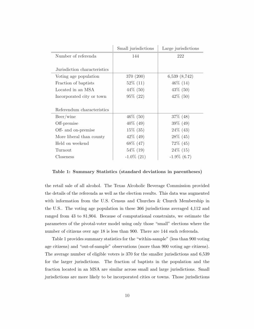
Table 1: Summary Statistics (standard deviations in parentheses)

the retail sale of all alcohol. The Texas Alcoholic Beverage Commission provided

the details of the referenda as well as the election results. This data was augmented

with information from the U.S. Census and Churches & Church Membership in

the U.S.. The voting age population in these 366 jurisdictions averaged 4,112 and

ranged from 43 to 81,904. Because of computational constraints, we estimate the

parameters of the pivotal-voter model using only those “small” elections where the

number of citizens over age 18 is less than 900. There are 144 such referenda.

Table 1 provides summary statistics for the “within-sample” (less than 900 voting

age citizens) and “out-of-sample” observations (more than 900 voting age citizens).

The average number of eligible voters is 370 for the smaller jurisdictions and 6,539

for the larger jurisdictions. The fraction of baptists in the population and the

fraction located in an MSA are similar across small and large jurisdictions. Small

jurisdictions are more likely to be incorporated cities or towns. Those jurisdictions

10

0

20

40

60

80

100

Turn

out

0 10000 20000 30000 40000

Eligible voters

Data

Polynomial fit

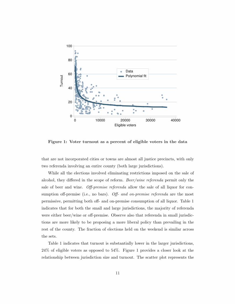
Figure 1: Voter turnout as a percent of eligible voters in the data

that are not incorporated cities or towns are almost all justice precincts, with only

two referenda involving an entire county (both large jurisdictions).

While all the elections involved eliminating restrictions imposed on the sale of

alcohol, they differed in the scope of reform. Beer/wine referenda permit only the

sale of beer and wine. Off-premise referenda allow the sale of all liquor for con-

sumption off-premise (i.e., no bars). Off- and on-premise referenda are the most

permissive, permitting both off- and on-premise consumption of all liquor. Table 1

indicates that for both the small and large jurisdictions, the majority of referenda

were either beer/wine or off-premise. Observe also that referenda in small jurisdic-

tions are more likely to be proposing a more liberal policy than prevailing in the

rest of the county. The fraction of elections held on the weekend is similar across

the sets.

Table 1 indicates that turnout is substantially lower in the larger jurisdictions,

24% of eligible voters as opposed to 54%. Figure 1 provides a closer look at the

relationship between jurisdiction size and turnout. The scatter plot represents the

11

0

.02

.04

.06

.08

Density

−50 0 50

Closeness

Small jurisdictions

Large jurisdictions

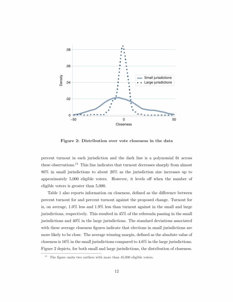
Figure 2: Distribution over vote closeness in the data

percent turnout in each jurisdiction and the dark line is a polynomial fit across

these observations.11 This line indicates that turnout decreases sharply from almost

80% in small jurisdictions to about 20% as the jurisdiction size increases up to

approximately 5,000 eligible voters. However, it levels off when the number of

eligible voters is greater than 5,000.

Table 1 also reports information on closeness, defined as the difference between

percent turnout for and percent turnout against the proposed change. Turnout for

is, on average, 1.0% less and 1.9% less than turnout against in the small and large

jurisdictions, respectively. This resulted in 45% of the referenda passing in the small

jurisdictions and 40% in the large jurisdictions. The standard deviations associated

with these average closeness figures indicate that elections in small jurisdictions are

more likely to be close. The average winning margin, defined as the absolute value of

closeness is 16% in the small jurisdictions compared to 4.6% in the large jurisdictions.

Figure 2 depicts, for both small and large jurisdictions, the distribution of closeness.

11 The figure omits two outliers with more than 45,000 eligible voters.

12

The solid line shows the kernel density estimate of the closeness of the referendum

outcomes in small jurisdictions while the dashed line is the kernel density estimate

for the larger jurisdictions. Figure 2 indicates that there is considerable variation

in closeness across jurisdictions and that this variation is greater for the smaller

jurisdictions.12

4 Estimation

4.1 Identification

Our goal is to provide inference on the parameters of the model using the data

on election outcomes in Texas liquor referenda. Before describing in detail the

estimation procedure, it is important to discuss what features of the data allow us

to identify the coefficients associated with the model’s parameters. Recall that the

model outlined in section 2 is characterized by just four parameters: the supporters’

benefit b; the opposers’ loss x; the probability that a citizen is a supporter µ; and

the upper bound of the uniform cost distribution, c. We will consider how changes

in the values of the parameters impact the outcome predicted by the model.

To simplify the discussion, assume that all jurisdictions share the same values

of b, x, µ, and c. Note first that only the relative values of b, x, and c matter;

that is, when b, x, and c are multiplied by the same factor, the equilibrium values

of γs and γo are also scaled by the same factor, and the probability of observing

a referendum outcome (the number of votes for and against) conditional on the

equilibrium cut-off levels is independent of the scaling factor. Therefore, under the

simplifying assumption that all jurisdictions are identical, c is not identified, and we

can normalize c to 1.

Next observe that the combined magnitude of parameters b and x effects overall

turnout, because increasing the benefits from winning the election increases the

incentives to vote, and therefore turnout. What is left is the determination of the

difference b−x and µ. Both b−x and µ are identified from the observed difference

12 This pattern remains when the jurisdictions are broken into smaller subsamples based onnumber of eligible voters.

13

between turnout for and turnout against. We are able to separately identify b − x

and µ because: (i) a change in b − x has different effects than a change in µ on

turnout; and (ii) the differential effects of changes in b− x and µ vary with the size

of the jurisdiction and total turnout. For example, the difference between votes for

and against provides more information on µ relative to b − x when a jurisdiction

has high total turnout and a large number of eligible voters. Hence, variation in

closeness of the electoral outcome across jurisdictions with different levels of turnout

and different numbers of eligible voters facilitate the identification of µ from b− x.

We conclude that, under the assumption that all jurisdictions have identical b,

x, µ, and c, identification of these parameters is possible (after normalizing the

cost of voting) provided that sufficient variation exists across jurisdictions in eligi-

ble voters and referendum outcome. In our empirical implementation, we allow the

four parameters to have different values by having them depend on exogenous ju-

risdiction characteristics. The coefficients associated with these jurisdiction specific

variables are identified from the variation in electoral outcomes across jurisdictions

with different exogenous characteristics.

4.2 Estimation procedure

We assume that each of our 144 jurisdictions is characterized by a distinct quadruple

of parameters (µj ,bj ,xj ,cj) but that each parameter is determined by jurisdiction and

referenda specific characteristics in a common way. Specifically, for each jurisdiction

j, we assume that:

bj = exp(βb · zb

j

)(9)

xj = exp(βx · zx

j

)(10)

µj =exp

(βµ · zµ

j

)

1 + exp(βµ · zµ

j

) (11)

cj = exp(βc · zc

j

)(12)

where (βb, βx, βµ, βc) are vectors of coefficients to be determined and (zbj , z

xj , zµ

j , zcj)

are vectors of observable jurisdiction and referenda characteristics. More specifically,

zbj = zx

j =(1, off-premise, off- and on-premise, incorporated city or town, more liberal

14

than county), zµj = (1, fraction baptist, MSA), and zc

j =(election on weekend). The

functional forms for bj , xj and cj are selected so that they are positive and the

functional form for µj is selected to ensure that it lies between zero and one. The

formulation also embodies the normalization that cj equals 1 when the election is

not held on the weekend.

The task is to estimate the coefficients (βb, βx, βµ, βc). For each jurisdiction j

we observe the votes for and against the proposed change, together with the total

number of eligible voters which we denote respectively as vsj , voj , and nj . The choice

of (βb, βx, βµ, βc) determine bj , xj , µj and cj and these determine via equations (2)

and (4) a set of Mj equilibria in each jurisdiction j, which we denote γmsj , γ

mojMj

m=1.

Each equilibrium implies a probability distribution over election outcomes. In

particular, the probability of observing data (vsj , voj) conditional on the citizens

voting according to the cut-off levels (γsj , γoj) is given by (8). While it is impossible

to know a priori whether there are multiple equilibria, if there is multiplicity we need

to ensure that there is a unique mapping from the parameter space to the likelihood

of observable events. We resolve this issue by assuming that the equilibrium selected

is the first equilibrium the computation routine finds, using as a starting point of

the routine the midpoint of the strategy space.13

Assuming the above equilibrium selection rule, denote the selected equilibrium

(γm∗sj , γm∗

oj ). Then, equation (8) defines the likelihood of observing a referendum

outcome conditional on the equilibrium cut-off levels (γm∗sj , γm∗

oj ). The likelihood

function is therefore

L(βb, βx, βµ, βc) =∏

j

ρ(vsj , voj ; γm∗sj , γm∗

oj ). (13)

The estimation strategy is the following: first, guess a vector of coefficient values (βb,

βx, βµ, βc). Then compute equilibrium critical cost levels for each jurisdiction (based

13 An alternative procedure is to assume an equilibrium selection rule, and estimate the param-eters of the equilibrium selection rule together with the parameters of the model. We experimentedwith this procedure, but found it computationally unfeasible. The procedure we chose is arbitraryonly to the extent in which multiplicity is prevalent. We investigated this issue and found that mul-tiplicity does not arise very often. We thoroughly searched for equilibria using a grid of parametervectors centered around our estimates. For all of these parameter vectors, we found multiplicity inless than ten percent of the jurisdictions. At the estimated values of the parameters, we found only7 jurisdictions displaying multiple equilibria.

15

on the equilibrium selection rule stated above), and the probability of observing the

jurisdiction election outcome conditional on such thresholds. These probabilities

determine the likelihood of observing the data given by L(βb, βx, βµ, βc). Finally,

find the coefficient values that maximize L(βb, βx,βµ, βc).

The sums in equations (2), (4), and (8) take progressively longer to compute as

the number of eligible voters increases, making the computation of the equilibria

extremely time consuming in large jurisdictions, even using Normal approximations

to the Binomial distributions. This explains why we limited our sample to the 144

observations with the smallest number of eligible voters.14

5 Results

5.1 Coefficient estimates

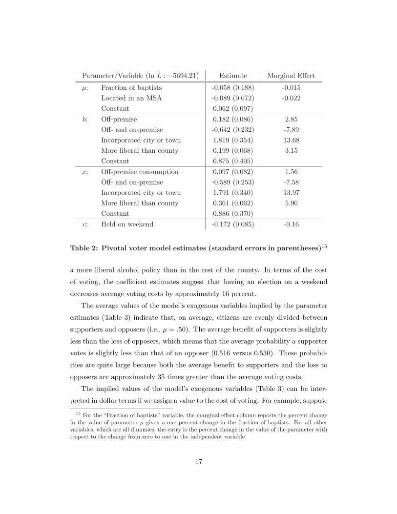
Table 2 contains the coefficient values that maximize the likelihood function, with

bootstrapped standard errors in parentheses, while Table 3 provides the average

values of the model’s exogenous variables implied by these parameter estimates.

The point estimates in Table 2 suggest that the probability an individual is a

supporter does not depend appreciably on the fraction of baptists in the jurisdic-

tion or on whether the jurisdiction is located in an MSA. The coefficient estimates

associated with the benefit and loss parameters, b and x, suggest that the effect of

the jurisdiction-specific characteristics on preferences are often quite large and sim-

ilar for supporters and opposers. Both supporters and opposers benefit more from

their preferred outcome if the jurisdiction holding the election is an incorporated

city or town. Less intuitively, both groups’ benefits are less for off- and on-premise

referenda compared to off-premise referenda and beer/wine referenda (the omitted

category). The average supporter’s benefit and opposer’s loss almost double when

the jurisdiction is a city/town and are approximately fifty percent less for an off-

and on-premise referendum than a beer/wine referendum. The benefit and loss pa-

rameters increase slightly if the referendum passing results in the jurisdiction having

14 We used an implementation of the simulated annealing method developed by Bill Goffe (seeGoffe et al. (1992)) to maximize (13) on a 16-processor supercomputer.

16

Parameter/Variable (ln L : −5694.21) Estimate Marginal Effect

µ: Fraction of baptists -0.058 (0.188) -0.015Located in an MSA -0.089 (0.072) -0.022Constant 0.062 (0.097)

b: Off-premise 0.182 (0.086) 2.85Off- and on-premise -0.642 (0.232) -7.89Incorporated city or town 1.819 (0.354) 13.68More liberal than county 0.199 (0.068) 3.15Constant 0.875 (0.405)

x: Off-premise consumption 0.097 (0.082) 1.56Off- and on-premise -0.589 (0.253) -7.58Incorporated city or town 1.791 (0.340) 13.97More liberal than county 0.361 (0.062) 5.90Constant 0.886 (0.370)

c: Held on weekend -0.172 (0.085) -0.16

Table 2: Pivotal voter model estimates (standard errors in parentheses)15

a more liberal alcohol policy than in the rest of the county. In terms of the cost

of voting, the coefficient estimates suggest that having an election on a weekend

decreases average voting costs by approximately 16 percent.

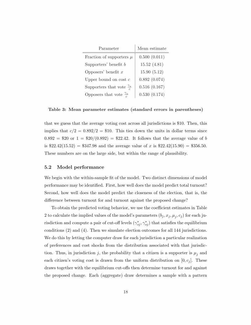
The average values of the model’s exogenous variables implied by the parameter

estimates (Table 3) indicate that, on average, citizens are evenly divided between

supporters and opposers (i.e., µ = .50). The average benefit of supporters is slightly

less than the loss of opposers, which means that the average probability a supporter

votes is slightly less than that of an opposer (0.516 versus 0.530). These probabil-

ities are quite large because both the average benefit to supporters and the loss to

opposers are approximately 35 times greater than the average voting costs.

The implied values of the model’s exogenous variables (Table 3) can be inter-

preted in dollar terms if we assign a value to the cost of voting. For example, suppose

15 For the “Fraction of baptists” variable, the marginal effect column reports the percent changein the value of parameter µ given a one percent change in the fraction of baptists. For all othervariables, which are all dummies, the entry is the percent change in the value of the parameter withrespect to the change from zero to one in the independent variable.

17

Parameter Mean estimate

Fraction of supporters µ 0.500 (0.011)

Supporters’ benefit b 15.52 (4.81)

Opposers’ benefit x 15.90 (5.12)

Upper bound on cost c 0.892 (0.074)

Supporters that vote γsc 0.516 (0.167)

Opposers that vote γoc 0.530 (0.174)

Table 3: Mean parameter estimates (standard errors in parentheses)

that we guess that the average voting cost across all jurisdictions is $10. Then, this

implies that c/2 = 0.892/2 = $10. This ties down the units in dollar terms since

0.892 = $20 or 1 = $20/(0.892) = $22.42. It follows that the average value of b

is $22.42(15.52) = $347.98 and the average value of x is $22.42(15.90) = $356.50.

These numbers are on the large side, but within the range of plausibility.

5.2 Model performance

We begin with the within-sample fit of the model. Two distinct dimensions of model

performance may be identified. First, how well does the model predict total turnout?

Second, how well does the model predict the closeness of the election, that is, the

difference between turnout for and turnout against the proposed change?

To obtain the predicted voting behavior, we use the coefficient estimates in Table

2 to calculate the implied values of the model’s parameters (bj , xj , µj , cj) for each ju-

risdiction and compute a pair of cut-off levels (γ∗sj , γ∗oj) that satisfies the equilibrium

conditions (2) and (4). Then we simulate election outcomes for all 144 jurisdictions.

We do this by letting the computer draw for each jurisdiction a particular realization

of preferences and cost shocks from the distribution associated with that jurisdic-

tion. Thus, in jurisdiction j, the probability that a citizen is a supporter is µj and

each citizen’s voting cost is drawn from the uniform distribution on [0, cj ]. These

draws together with the equilibrium cut-offs then determine turnout for and against

the proposed change. Each (aggregate) draw determines a sample with a pattern

18

Eligible voters n N. of obs. DataPivotal-voter

model

n < 247 48 0.62 0.65

247 < n < 434 48 0.55 0.51

434 < n < 900 48 0.43 0.40

All within-sample (n < 900) 144 0.54 0.52

Table 4: Average turnout as a percentage of eligible voters: model vs.

data

of election outcomes across the jurisdictions. By repeating the procedure numerous

times and averaging across all samples we can compute the predicted distributions

for total turnout and closeness implied by the model.

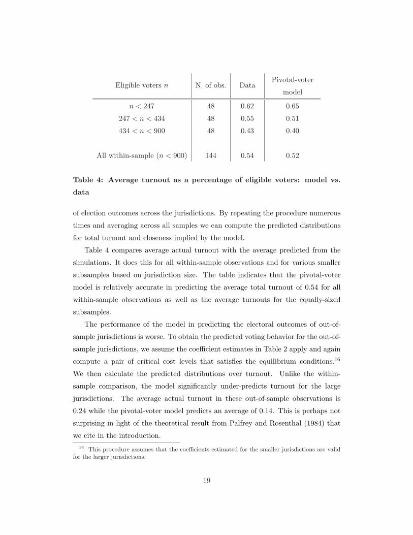
Table 4 compares average actual turnout with the average predicted from the

simulations. It does this for all within-sample observations and for various smaller

subsamples based on jurisdiction size. The table indicates that the pivotal-voter

model is relatively accurate in predicting the average total turnout of 0.54 for all

within-sample observations as well as the average turnouts for the equally-sized

subsamples.

The performance of the model in predicting the electoral outcomes of out-of-

sample jurisdictions is worse. To obtain the predicted voting behavior for the out-of-

sample jurisdictions, we assume the coefficient estimates in Table 2 apply and again

compute a pair of critical cost levels that satisfies the equilibrium conditions.16

We then calculate the predicted distributions over turnout. Unlike the within-

sample comparison, the model significantly under-predicts turnout for the large

jurisdictions. The average actual turnout in these out-of-sample observations is

0.24 while the pivotal-voter model predicts an average of 0.14. This is perhaps not

surprising in light of the theoretical result from Palfrey and Rosenthal (1984) that

we cite in the introduction.16 This procedure assumes that the coefficients estimated for the smaller jurisdictions are valid

for the larger jurisdictions.

19

0

.02

.04

.06

.08

.1

De

nsity

−50 0 50

Closeness

Model

Data

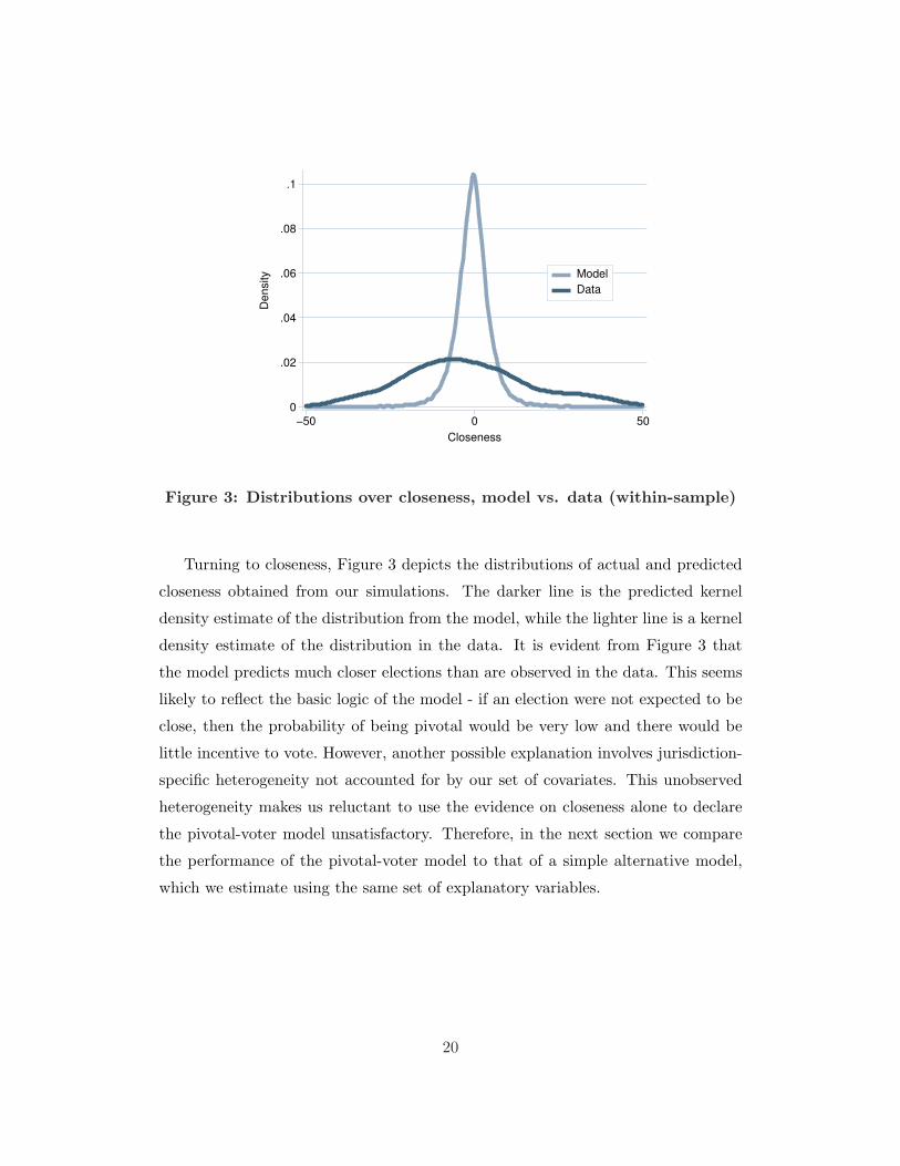
Figure 3: Distributions over closeness, model vs. data (within-sample)

Turning to closeness, Figure 3 depicts the distributions of actual and predicted

closeness obtained from our simulations. The darker line is the predicted kernel

density estimate of the distribution from the model, while the lighter line is a kernel

density estimate of the distribution in the data. It is evident from Figure 3 that

the model predicts much closer elections than are observed in the data. This seems

likely to reflect the basic logic of the model - if an election were not expected to be

close, then the probability of being pivotal would be very low and there would be

little incentive to vote. However, another possible explanation involves jurisdiction-

specific heterogeneity not accounted for by our set of covariates. This unobserved

heterogeneity makes us reluctant to use the evidence on closeness alone to declare

the pivotal-voter model unsatisfactory. Therefore, in the next section we compare

the performance of the pivotal-voter model to that of a simple alternative model,

which we estimate using the same set of explanatory variables.

20

6 A simple alternative model

While the pivotal-voter model yields reasonable coefficient estimates and fits the

pattern of turnout within-sample reasonably well, it predicts that elections will be

much closer than they actually are. It is therefore natural to wonder whether a

simpler model based on the idea of citizens voting for non-instrumental reasons

might fit the data better. To investigate this we study the comparative performance

of a simple expressive model of voting.

The expressive view asserts that citizens vote not to impact the outcome but

to express their preferences (see, for example, Brennan and Lomasky (1993)). It

seems natural to assume that people care more about expressing their preferences

the more intensely they feel about an issue. This suggests what Coate and Conlin

(2004) refer to as the intensity model which works within the same basic environment

as the pivotal-voter model but assumes that supporters vote if their voting cost is

less than γs = αb, while opposers vote if their voting cost is less than γo = αx, where

α > 0. Here, the parameter α measures the strength of citizens’ desire to express

themselves through voting. The key restriction is that both supporters and opposers

share the same α. Under this specification, the probability that a supporter votes

is the probability that γs exceeds his voting cost, which is γs/c = αb/c. Similarly,

the probability that an opposer votes is γo/c = αx/c. Note that, unlike the pivotal-

voter model, the propensity of a supporter (opposer) to vote does not depend on

the propensity of an opposer (supporter) to vote.

We assume that the parameters bj , xj , µj , and cj depend on the same jurisdiction

characteristics as in the pivotal-voter model (see equations 9-12). In addition, we

assume that:

αj = (number of eligible voters in jurisdiction j)β (14)

Thus, we allow citizens’ desire to express themselves to vary with the size of their

community. Observe that our specification for αj contains no constant term. This

normalization reflects the fact that we cannot separately identify αj , bj and xj . The

effect on voting behavior of an increase in the desire of citizens to express themselves

(i.e., an increase in αj) can be mimicked by an increase in how strongly they feel

21

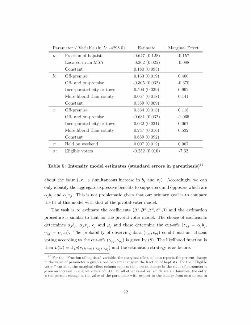
Parameter / Variable (ln L: -4298.0) Estimate Marginal Effect

µ: Fraction of baptists -0.647 (0.128) -0.157Located in an MSA -0.362 (0.025) -0.088Constant 0.180 (0.095)

b: Off-premise 0.163 (0.019) 0.406Off- and on-premise -0.305 (0.032) -0.670Incorporated city or town 0.504 (0.039) 0.992More liberal than county 0.057 (0.018) 0.141Constant 0.359 (0.069)

x: Off-premise 0.554 (0.015) 0.118Off- and on-premise -0.631 (0.032) -1.065Incorporated city or town 0.032 (0.031) 0.067More liberal than county 0.247 (0.016) 0.532Constant 0.659 (0.092)

c: Held on weekend 0.007 (0.012) 0.007

α: Eligible voters -0.252 (0.010) -7.62

Table 5: Intensity model estimates (standard errors in parenthesis)17

about the issue (i.e., a simultaneous increase in bj and xj). Accordingly, we can

only identify the aggregate expressive benefits to supporters and opposers which are

αjbj and αjxj . This is not problematic given that our primary goal is to compare

the fit of this model with that of the pivotal-voter model.

The task is to estimate the coefficients (βb, βx, βµ, βc, β) and the estimation

procedure is similar to that for the pivotal-voter model. The choice of coefficients

determines αjbj , αjxj , cj and µj and these determine the cut-offs (γsj = αjbj ,

γoj = αjxj). The probability of observing data (vsj , voj) conditional on citizens

voting according to the cut-offs (γsj , γoj) is given by (8). The likelihood function is

then L(Ω) = Πjρ(vsj , voj ; γsj , γoj) and the estimation strategy is as before.

17 For the “Fraction of baptists” variable, the marginal effect column reports the percent changein the value of parameter µ given a one percent change in the fraction of baptists. For the ”Eligiblevoters” variable, the marginal effect column reports the percent change in the value of parameter αgiven an increase in eligible voters of 100. For all other variables, which are all dummies, the entryis the percent change in the value of the parameter with respect to the change from zero to one in

22

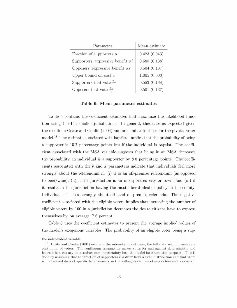
Parameter Mean estimate

Fraction of supporters µ 0.423 (0.043)

Supporters’ expressive benefit αb 0.585 (0.138)

Opposers’ expressive benefit αx 0.504 (0.137)

Upper bound on cost c 1.005 (0.003)

Supporters that vote γsc 0.583 (0.138)

Opposers that vote γoc 0.501 (0.137)

Table 6: Mean parameter estimates

Table 5 contains the coefficient estimates that maximize this likelihood func-

tion using the 144 smaller jurisdictions. In general, these are as expected given

the results in Coate and Conlin (2004) and are similar to those for the pivotal-voter

model.18 The estimate associated with baptists implies that the probability of being

a supporter is 15.7 percentage points less if the individual is baptist. The coeffi-

cient associated with the MSA variable suggests that being in an MSA decreases

the probability an individual is a supporter by 8.8 percentage points. The coeffi-

cients associated with the b and x parameters indicate that individuals feel more

strongly about the referendum if: (i) it is an off-premise referendum (as opposed

to beer/wine); (ii) if the jurisdiction is an incorporated city or town; and (iii) if

it results in the jurisdiction having the most liberal alcohol policy in the county.

Individuals feel less strongly about off- and on-premise referenda. The negative

coefficient associated with the eligible voters implies that increasing the number of

eligible voters by 100 in a jurisdiction decreases the desire citizens have to express

themselves by, on average, 7.6 percent.

Table 6 uses the coefficient estimates to present the average implied values of

the model’s exogenous variables. The probability of an eligible voter being a sup-

the independent variable.18 Coate and Conlin (2004) estimate the intensity model using the full data set, but assume a

continuum of voters. The continuum assumption makes votes for and against deterministic andhence it is necessary to introduce some uncertainty into the model for estimation purposes. This isdone by assuming that the fraction of supporters is a draw from a Beta distribution and that thereis unobserved district specific heterogeneity in the willingness to pay of supporters and opposers.

23

Eligible voters n N of Obs. DataIntensity

model

n < 247 48 0.62 0.63

247 < n < 434 48 0.55 0.53

434 < n < 900 48 0.43 0.45

All within-sample (n < 900) 144 0.54 0.54

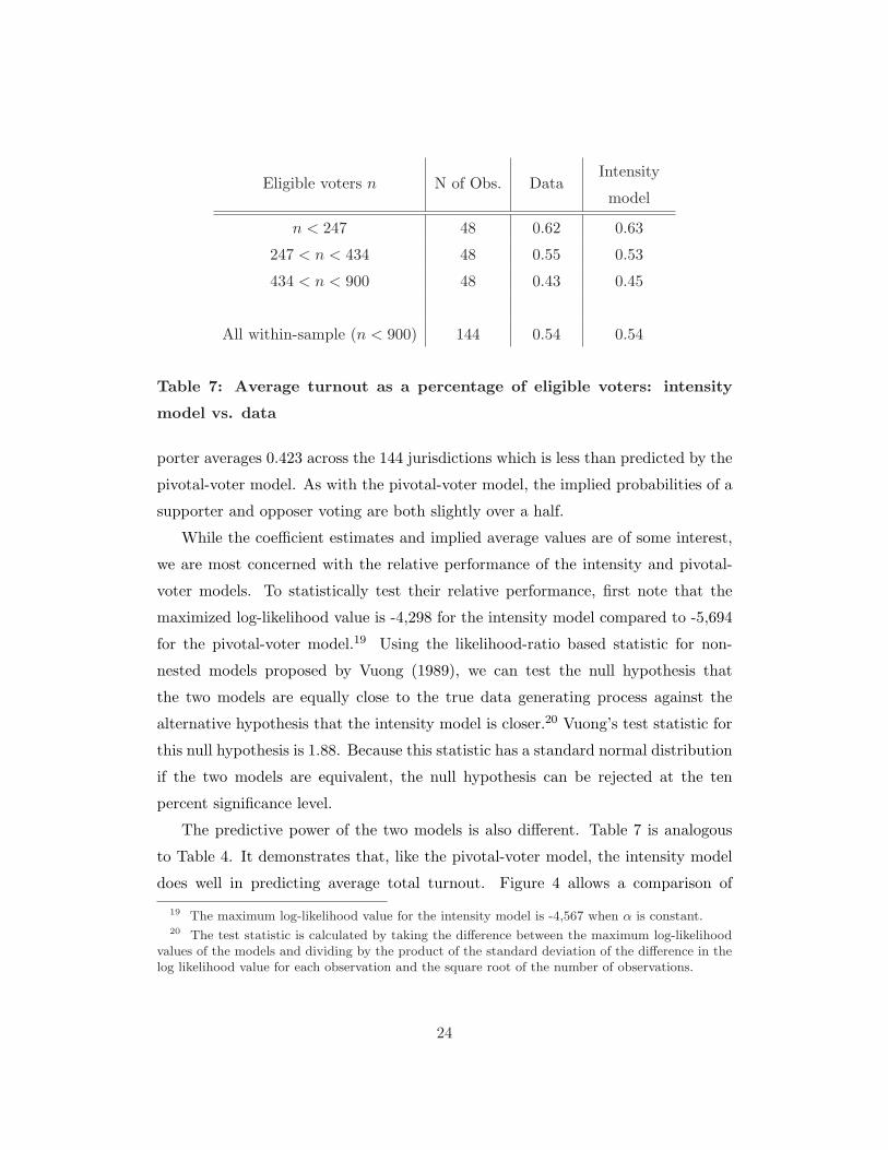
Table 7: Average turnout as a percentage of eligible voters: intensity

model vs. data

porter averages 0.423 across the 144 jurisdictions which is less than predicted by the

pivotal-voter model. As with the pivotal-voter model, the implied probabilities of a

supporter and opposer voting are both slightly over a half.

While the coefficient estimates and implied average values are of some interest,

we are most concerned with the relative performance of the intensity and pivotal-

voter models. To statistically test their relative performance, first note that the

maximized log-likelihood value is -4,298 for the intensity model compared to -5,694

for the pivotal-voter model.19 Using the likelihood-ratio based statistic for non-

nested models proposed by Vuong (1989), we can test the null hypothesis that

the two models are equally close to the true data generating process against the

alternative hypothesis that the intensity model is closer.20 Vuong’s test statistic for

this null hypothesis is 1.88. Because this statistic has a standard normal distribution

if the two models are equivalent, the null hypothesis can be rejected at the ten

percent significance level.

The predictive power of the two models is also different. Table 7 is analogous

to Table 4. It demonstrates that, like the pivotal-voter model, the intensity model

does well in predicting average total turnout. Figure 4 allows a comparison of

19 The maximum log-likelihood value for the intensity model is -4,567 when α is constant.20 The test statistic is calculated by taking the difference between the maximum log-likelihood

values of the models and dividing by the product of the standard deviation of the difference in thelog likelihood value for each observation and the square root of the number of observations.

24

0

.05

.1

−50 0 50−50 0 50

Pivotal−voter model Intensity model

Model

Data

De

nsity

Closeness

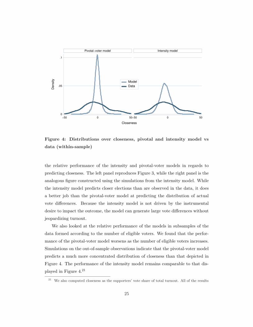
Figure 4: Distributions over closeness, pivotal and intensity model vs

data (within-sample)

the relative performance of the intensity and pivotal-voter models in regards to

predicting closeness. The left panel reproduces Figure 3, while the right panel is the

analogous figure constructed using the simulations from the intensity model. While

the intensity model predicts closer elections than are observed in the data, it does

a better job than the pivotal-voter model at predicting the distribution of actual

vote differences. Because the intensity model is not driven by the instrumental

desire to impact the outcome, the model can generate large vote differences without

jeopardizing turnout.

We also looked at the relative performance of the models in subsamples of the

data formed according to the number of eligible voters. We found that the perfor-

mance of the pivotal-voter model worsens as the number of eligible voters increases.

Simulations on the out-of-sample observations indicate that the pivotal-voter model

predicts a much more concentrated distribution of closeness than that depicted in

Figure 4. The performance of the intensity model remains comparable to that dis-

played in Figure 4.21

21 We also computed closeness as the supporters’ vote share of total turnout. All of the results

25

7 Conclusion

The pivotal-voter model forms the basic framework for thinking about turnout in

theoretical political science. While it seems widely conceded that the model does

not provide an empirically satisfactory theory of turnout in large-scale, single-issue

elections, the hope has remained that it might explain voter behavior in small-scale

elections. It is this hope that seems to implicitly justify the continued use of the

model in theoretical work.

The results of this paper provide little to nurture this hope. While the pivotal-

voter model can explain turnout in small-scale Texas liquor elections, it has difficulty

explaining the large winning margins that are common in these elections. The

logic of the pivotal-voter model implies that elections must be close even if there

is a significant difference between the sizes of the two competing groups or the

intensity of their preferences. This difficulty in explaining large winning margins

allows the pivotal-voter model to be outperformed by the intensity model - a simple

expressive voting model which just assumes that people are more likely to vote the

more intensely they feel about the issue.

Using the same data set, Coate and Conlin (2004) have shown that a model

of voter turnout in which individuals are motivated to vote by ethical reasons, fits

the data well and outperforms the intensity model. Transitivity does not strictly

speaking apply, because Coate and Conlin’s analysis makes different assumptions,

most notably a continuum of voters. Nonetheless, the combined results of the two

papers certainly suggest that an ethical approach is a better way of understanding

voter behavior than the pivotal-voter model. In our view, this reinforces the case

for further development of the ethical approach.

References

[1] Borgers, Tilman, [2004] “Costly Voting,” American Economic Review, 94(1),

57-66.

are similar to the results obtained using the measure of closeness used in the paper. Details areavailable from the authors upon request.

26

[2] Brennan, Geoffrey and Loren Lomasky, [1993], Democracy and Decision: The

Pure Theory of Electoral Preference, Cambridge: Cambridge University Press.

[3] Campbell, Colin, [1999], “Large Electorates and Decisive Minorities,” Journal

of Political Economy, 107(6), 1199-1217.

[4] Coate, Stephen and Michael Conlin, [2004], “A Group Rule-Utilitarian Ap-

proach to Voter Turnout: Theory and Evidence,” American Economic Review,

forthcoming.

[5] Feddersen, Timothy J., [2004], “Rational Choice Theory and the Paradox of

Not Voting,” Journal of Economic Perspectives, 18(1), 99-112.

[6] Feddersen, Timothy J. and Alvaro Sandroni, [2002], “A Theory of Participation

in Elections,” mimeo, Northwestern University.

[7] Ghosal, Sayantan and Ben Lockwood, [2003], “Information Aggregation, Costly

Voting and Common Values,” mimeo, University of Warwick.

[8] Goffe, William L., Ferrier, Gary D and Rogers, John [1992], “Simulated Anneal-

ing: An Initial Application in Econometrics,” Computer Science in Economics

& Management, 5(2), 133-46.

[9] Green, Donald and Ian Shapiro, [1994], Pathologies of Rational Choice Theory:

A Critique of Applications in Political Science, New Haven: Yale University

Press.

[10] Hansen, Stephen; Palfrey, Thomas and Howard Rosenthal, [1987], “The Down-

sian Model of Electoral Participation: Formal Theory and Empirical Analysis

of the Constituency Size Effect,” Public Choice, 52, 15-33.

[11] Harsanyi, John C., [1980], “Rule Utilitarianism, Rights, Obligations and the

Theory of Rational Behavior,” Theory and Decision, 12, 115-33.

[12] Ledyard, John O., [1984], “The Pure Theory of Large Two-Candidate Elec-

tions,” Public Choice, 44, 7-41.

27

[13] Palfrey, Thomas and Howard Rosenthal, [1983], “A Strategic Calculus of Vot-

ing,” Public Choice, 41, 7-53.

[14] Palfrey, Thomas and Howard Rosenthal, [1985], “Voter Participation and

Strategic Uncertainty,” American Political Science Review, 79, 62-78.

[15] Vuong, Quang H., [1989], “Likelihood Ratio Tests for Model Selection and

Non-nested Hypotheses,” Econometrica, 57, 307-333.

28