NBER WORKING PAPER SERIES

SOME EVIDENCE ON THE IMPORTANCE OF STICKY PRICES

Mark Bils

Peter J. Klenow

Working Paper 9069

http://www.nber.org/papers/w9069

NATIONAL BUREAU OF ECONOMIC RESEARCH

1050 Massachusetts Avenue

Cambridge, MA 02138

July 2002

We are grateful to Sreya Kolay and especially Oleksiy Kryvtsov for excellent research assistance. We thank

Walter Lane and John Greenlees for providing us with unpublished BLS data. For helpful suggestions we

thank Susanto Basu, Michael Bryan, Jeff Campbell, Alan Kackmeister, Ananth Sheshadri, and Guhan

Venkatu. The views expressed herein are those of the authors and not necessarily those of the National

Bureau of Economic Research.

© 2002 by Mark Bils and Peter J. Klenow. All rights reserved. Short sections of text, not to exceed two

paragraphs, may be quoted without explicit permission provided that full credit, including © notice, is given

to the source.

Some Evidence on the Importance of Sticky Prices

Mark Bils and Peter J. Klenow

NBER Working Paper No. 9069

July 2002

JEL No. E31, E32, L11

ABSTRACT

We examine the frequency of price changes for 350 categories of goods and services covering

about 70% of consumer spending, based on unpublished data from the BLS for 1995 to 1997. Compared

with previous studies we find much more frequent price changes, with half of prices lasting less than 4.3

months. The frequency of price changes differs dramatically across categories. We exploit this variation

to ask how inflation for "flexible-price goods" (goods with frequent changes in individual prices) differs

from inflation for "sticky-price goods" (those displaying infrequent price changes). Compared to the

predictions of popular sticky price models, actual inflation rates are far more volatile and transient,

particularly for sticky-price goods.

Mark Bils Peter J. Klenow

Department of Economics Research Department

University of Rochester Federal Reserve Bank of Minneapolis

Rochester, NY 14627 90 Hennepin Avenue

and NBER Minneapolis, MN 55480-0291

bils@troi.cc.rochester.edu and NBER

pete@klenow.com

1

1. Introduction

The importance of price stickiness remains a central question in economics. After a ten-

year period of relative quiet, sticky-price models are again at, or near, the center of analysis of

business cycle fluctuations and monetary policy. Goodfriend and King (1997), Rotemberg and

Woodford (1997), Clarida, Gali, and Gertler (1999), Erceg, Henderson, and Levin (2000), Chari,

Kehoe, and McGrattan (2000), Christiano, Eichenbaum, and Evans (2001), and Dotsey and King

(2001) are examples of recent work built on the assumptions that firms adjust prices infrequently

and satisfy all demand at those posted prices.

With the exception of Dotsey and King (2001), these studies employ time-dependent

pricing. Prices are maintained for a set number of periods (as in Taylor, 1999) or each period

a fixed fraction of firms have an opportunity to adjust prices to new information (as in Calvo,

1983). In both the Taylor and Calvo models price changes are not synchronized across firms.

In these settings monetary policy can influence economic activity for some period of time. By

contrast, Caplin and Spulber (1987) illustrate that state-dependent models of price changes

generate less clear predictions for the impact of monetary policy on real activity. As we

discuss at length, models with staggered time-dependent pricing imply that inflation rates

should be more persistent and less volatile if price changes are less frequent.

The speed with which sticky-price models were first jettisoned then retrieved partly

reflects the lack of conclusive evidence on the extent and importance of sticky prices. Several

papers have shown that certain wholesale and retail prices often go unchanged for many

months (Carlton, 1986, Cecchetti, 1986, Kashyap, 1995, Levy, Bergen, Dutta and Venable,

1997, Blinder, Canetti, Lebow and Rudd, 1998, MacDonald and Aaronson, 2001, and

Kackmeister, 2001). Compared to these studies, we obtain broader evidence on the extent of

retail price rigidities and their consequences for the behavior of inflation. We employ

unpublished data from the U.S. Bureau of Labor Statistics (BLS) for 1995 to 1997 on the

monthly frequency of price changes for 350 categories of consumer goods and services

comprising around 70% of consumer expenditures. We find that many prices seldom change.

2

Prices of newspapers, men's haircuts, and taxi fares change less than 5% of months. By

contrast, many prices change very frequently. The prices of gasoline, tomatoes, and airfares

change more than 70% of months. We exploit this diversity. We classify goods by how

frequently they display monthly price changes in the 1995-1997 data, then ask how the

behavior of inflation differs between goods with frequent versus infrequent price changes.

In the next section (section 2) we present the disaggregate data on the frequency of

price changes for 1995 to 1997. We contrast our findings to the existing literature. We find

much more frequent price changes, with half of prices lasting 4.3 months or less. We also

present a number of characteristics that predict whether a good will display a flexible price.

We find that variables capturing the volatility of market supply and demand can account for

much of the variation in price flexibility across categories. For example, goods that exhibit

frequent model changes typically exhibit flexible pricing.

In section 3 we briefly sketch a general equilibrium sticky-price model that follows

work in Chari, Kehoe and McGrattan (2000). They model monopolistically competitive firms

with staggered price setting of a fixed duration (a la Taylor, 1999). The wrinkle we add is

multiple consumer goods with prices fixed for different durations across the goods. We

simulate this model to illustrate how flexible-price goods and sticky-price goods can differ in

their responses to shocks.1

In section 4 we analyze monthly time series on prices and consumption for 123 goods

of varying price stickiness. In the workhorse Calvo and Taylor models, price stickiness

dampens the initial response of a good's inflation rate to a shock, stretching the inflation

impact out over time as successive cohorts of firms adjust their prices. Price stickiness

thereby reduces the magnitude of innovations to a good's inflation rate while, at the same

time, raising the persistence of its inflation. We do not see this in the data. For nearly all 123

categories, inflation movements are far more volatile and transient than implied by the Calvo

and Taylor models given the frequency of individual price changes in the BLS data. This

1 Several papers have incorporated sticky-price and flexible-price sectors into model economies. Examplesinclude Ohanian, Stockman, and Kilian (1995), Aoki (2001), and Benigno (2001).

3

discrepancy cannot be resolved by adding plausible measurement error or idiosyncratic

shocks. Across the 123 goods, volatility and persistence of a good's inflation rate are much

less related to the good's underlying frequency of price changes than predicted by these time-

dependent pricing models. In other words, the popular sticky-price models fail most

dramatically to predict inflation's behavior for goods with the least frequent price changes.

The final section (section 5) summarizes and discusses directions for further work.

2. BLS Data on the Frequency of Price Changes

For calculating the CPI, the BLS collects prices on 70,000 to 80,000 non-housing

goods and services per month. They collect these from around 22,000 outlets across 882

geographic areas. The BLS chooses outlets probabilistically based on household point-of-

purchase surveys, and choose items within outlets based on estimates of their relative sales.

The BLS divides consumption into 388 categories called Entry Level Items (ELIs).

The BLS gives, for each ELI, theCommodities and Services Substitution Rate Table

percentage of quotes with price changes. For example, the 1997 indicates that 6,493Table

price quotes were collected on bananas in 1997, and that 37.8% of these quotes differed from

the quote on the same type of bananas at the same outlet in the preceding month. (The Table

does not contain information on the magnitude of price changes, just what share of price

quotes involved change in price.) The field agents collecting prices use a detailedsome

checklist of item attributes to try to make sure they are pricing the same item in consecutive

months. When they cannot find an item, they substitute the price of a closely-related item at

the outlet. These "item substitutions" are the focus of the BLS , and we discuss them inTable

detail later in this section. Item substitutions happen to be rare for bananas (only 1 in 1997)

compared to other categories (3.1% of non-housing price quotes in 1997).

The BLS has provided us with the unpublished Commodities and Services Substitution

Rate Table for the years 1995 through 2001. The BLS revised the ELI structure in 1998, so

2 The sources used for this section, unless otherwise noted, were (1986) and theThe Boskin Commission ReportBLS Handbook of Methods (U.S. Department of Labor, 1997, Chapter 17).

4

frequencies cannot be readily compared before and after 1998. For the 168 ELI definitions

which remained unchanged, however, the frequencies are quite stable over the seven years.

The correlation for any pair of years lies between 0.96 and 0.98. In order to maximize the

number of ELIs for which there is a price index covering more than a few years, we use the

1995-1997 BLS data and its ELI structure. This data covers 350 ELIs.

In Table 1 we list, for each of the 350 ELIs, the 1995-1997 average frequencymonthly

of price changes. For food and energy ELIs, in which items are priced monthly, this is the

simple average of the frequencies in the 1995, 1996, and 1997 BLS . For the otherTables

ELIs, the frequencies in the BLS are a mixture of one-month and two-month priceTables

change frequencies. In the five largest areas — New York City and suburbs, Chicago, Los

Angeles and suburbs, San Francisco / Oakland / San Jose, and Philadelphia — the BLS

collects quotes monthly for all goods and services. For the other geographic areas, the BLS

collects quotes monthly only for food and energy, and bimonthly for all other goods and

services. For each of 1995, 1996 and 1997, we obtained from the BLS the fraction of price

quotes that were monthly vs. bimonthly.

If the monthly probability of a price change is the same across areas and from month

to month for a given ELI in a given year, then we can identify the monthly frequency of price

changes from the mixed frequency the BLS reports and the fraction of quotes which are

monthly versus bimonthly. In doing so we assume that the probability of a price changing

from to ne month, then changing Based on scannerp p back p � � �o to the next month, is zero.

data for select seasonal goods at certain Chicago-area supermarkets, Chevalier, Kashyap and

Rossi (2000) find that such temporary sales are actually quite common. To the extent they

occur, our estimated monthly frequencies understate the true monthly frequencies. Since

Chevalier et al. find that temporary sales typically last one week or less, even monthly price

quotes (as for the top five areas and for food and energy) understate the true frequency of

price changes. As we discuss later in this section, however, one could argue that temporary

sales mask the stickiness of "regular" prices.

5

Let the mixture of monthly and bimonthly frequencies (data from the BLS� =

Tables ), = the constant monthly frequency of price changes (not directly observed), and � �

= the fraction of quotes which are monthly (data we obtained from the BLS for each ELI for

each year). Then = * + (1– )*( + (1– )* ). Since z (0, 1) and [0,1], they z z� � � � �� �

solution for is the negative root of this quadratic in . Table 1 reports for each of the 350� � �

ELIs. These are averages of the monthly frequencies we estimate for 1995, 1996 and 1997.

They range from 1.2% for coin-operated apparel laundry and dry cleaning to 79% for regular

unleaded gasoline. Figure 1 gives the histogram of frequencies for the 350 ELIs. Not all ELIs

are equally important, however, as their weights in the 1995 Consumer Expenditure Survey

(CEX) range from 0.001% (tools and equipment for painting) to 2.88% for electricity. Table

1 also provides the weight of each ELI and the resulting percentile of the ELI in the

cumulative distribution of frequencies. Weighting the ELIs, the monthly frequency of price

changes averages 26.1%. The weighted median is 20.9%. For the median category the time

between price change averages 4.3 months. Thus, for items comprising one half of non-3

housing consumption, prices change less frequently than every 4.3 months.

The 350 ELIs in Table 1 cover 68.9% of spending according to the 1995 CEX. The

categories not covered are owner's equivalent rent and household insurance (20.0% weight),

residential rent (6.6%), used cars (1.8%), and various unpriced items (collectively 2.7%). One

question that arises is whether scanner data, which are becoming increasingly available to

economists (e.g., Chevalier et al., 2000), might dominate the BLS average frequency data.

Scanner data afford weekly prices and quantities for thousands of consumer items. At

present, however, scanner data cannot match the category coverage of the BLS data. Hawkes

and Piotrowski (2000) report that only 10% of consumer expenditures are scanned through

AC Nielsen data for supermarkets, drugstores, and mass merchandisers. Categories not

scanned include rent, utilities, restaurant meals (about 40% of spending on food), medical

3 If prices can change at any moment, not just at the monthly interval, the instantaneous probability of a pricechange is -ln(1- ) and the mean time between price changes -1/ln(1- ) months. We used this formula to� �

calculate the Mo. column from the Freq. column in Table 1. If prices instead change at most once per month,then the mean duration is simply 1/ , about half a month longer.�

6

care, transportation, insurance, banking, and education. As noted, the 350 categories in the

BLS cover 68.9% of consumer expenditures.Table

Table 2 reports the median frequency and duration for years 1995 through 2001. Price

changes are somewhat more frequent over 1998-2001 than over the 1995-1997 period we

focus on to maximize compatibility with other data.

Comparison to Other Empirical Studies of Price Stickiness

The BLS data suggests much more frequent price adjustment than has been found in

other studies. Blinder et al. (1998) surveyed 200 firms on their price setting. The median4

firm reported adjusting prices about once a year. Hall, Walsh and Yates (2000) surveyed 654

British companies and obtained similar results: 58% changing prices once a year or more. In

contrast, the median consumer item in the 1995-1997 BLS changes prices every 4.3Tables

months. For 87% of consumption prices change more frequently than once a year. A possible

contributor to the difference in findings is that firms in the Blinder et al. survey sell mostly

intermediate goods and services (79% of their sales) rather than consumer items.

Even compared to other studies of prices, the BLS data imply considerablyconsumer

more frequent price changes. Cecchetti (1986) studied newsstand prices of 38 American

magazines over 1953 to 1979. The number of years since the last price change ranged from

1.8 to 14 years. In our Table 1, magazines (including subscription as well as newsstand

prices) exhibit price changes 8.6% of months, implying adjustment every 11 months on

average. More importantly, magazines are at the sticky end of the spectrum in Table 1;

prices change more frequently than for magazines for 86% of non-housing consumption.

Kashyap (1995) studied the monthly prices of 12 mail-order catalog goods for periods

as long as 1953 to 1987. Across goods and time, he found an average of 14.7 months

between price changes. This contrasts with the 4.3 month median in the BLS data. Based on

Table 1, prices change more frequently than every 14.7 months for 90% of non-housing

4 The BLS data also suggest more frequent price adjustment than usually assumed in calibrated macro models.Chari et al. (2000), for instance, consider a benchmark case in which prices are set for one year.

7

consumption. The 12 Kashyap goods consist mostly of apparel. In the BLS data, prices

actually change more frequently for clothing: the monthly hazard is 29% for apparel items,

versus 26% for all items. So prices for the goods in Kashyap's sample are far stickier than the

typical BLS item, apparel or otherwise. Mail-order prices may tend to be stickier than prices

in retail outlets. Another factor could be that Kashyap selected "well-established, popular-

selling items that have undergone minimal quality changes" (Kashyap, 1995, p. 248). As we

discuss below, changing product features appear to play an important role in price changes.

MacDonald and Aaronson (2001) examine restaurant pricing (more exactly, pricing

for food consumed on premises) for the years 1995 to 1997 using BLS data. They find that

restaurant prices do not change very frequently, with prices displaying a median duration of

about 10 months. These are close to the durations we report for breakfast (11.4 months),

lunch (10.7), and dinner (10.6) prices in Table 1. This consistency is not surprising given we

are using the same underlying data source. Note, however, that prices change less frequently

at restaurants than for the typical good in the CPI bundle. Prices change more frequently than

for restaurant foods for about 80% of non-housing consumption.

Kackmeister (2001) analyzes data on the price levels of up to 49 consumer products

(depending on the period) in Los Angeles, Chicago, New York and Newark in 1889-1891,

1911-1913, and 1997-1999. The goods are at the ELI level or slightly more aggregated, and

include 27 food items, 14 home furnishing items, and 8 clothing items. He finds that the

frequency, size, and variability of price changes are higher in the last period than in the first

period. For 1997-1999 he finds that 31% of his goods change price each month. This is

higher than the mean frequency of 26% in our data; we conjecture the difference owes mostly

to the composition of goods rather than the sample period or cities.

With data on price levels, Kackmeister is able to investigate how often a price is

temporarily marked down from a "regular" price that is itself much stickier. He finds that

22% of prices change each month price reductions that reverse themselves oneexcluding

month later. If the same fraction (9/31) of price changes arose from temporary sales in our

8

data, then our mean frequency net of temporary sales would be 18% (vs. 26% including

temporary sales). The median time between changes in prices would be 6.2 monthsregular

(vs. 4.3 months with temporary sales). Even 6.2 months is considerably shorter than the 125

months or more found by previous studies. Moreover, one could argue that temporary sales

represent a true form of price flexibility that should not be filtered out, say because the

magnitude and duration of temporary sales responds to shocks.

Differences in Price Stickiness Across Broad Consumption Categories

Table 3 provides price change frequencies for selected broad categories of

consumption. The first row shows that the (weighted) mean frequency is 26% for all items.

The next three rows provide (weighted) mean frequencies for durable goods, nondurable

goods, and services, respectively, based on U.S. National Income and Product Account

(NIPA) classifications. Price changes are more frequent for goods (about 30% for both

durables and nondurables) than for services (21%). The lower frequency of price changes for

services could reflect the lower volatility of consumer demand for them.

The next six rows in Table 3 provide frequencies for each of the six CPI Expenditure

Classes defined by the BLS. At the flexible end are transportation prices (e.g., new cars,

airfares), almost 40% of which change monthly. At the sticky extreme are medical care

(drugs, physicians' services) and entertainment (admission prices, newspapers, magazines, and

books), for whom around 10% of prices change monthly.

In the final two rows of Table 3 we draw a distinction between "raw" and "processed"

goods. By raw goods we mean those with relatively little value added beyond a primary

input, for instance gasoline or fresh fruits and vegetables. Because their inputs are not well-

diversified, these goods may be subject to more volatile costs. Raw goods are a subset of the

5 According to the BLS, temporary sales are more common for food and clothing, the bulk of Kackmeister'ssample. For our sample, therefore, these calculations may overstate the effect of filtering out temporary sales.

9

food and energy items goods excluded by the BLS in its core rate of CPI inflation. As6

expected, raw products display more frequent price changes (their prices change 54% of

months) than do processed products and services (whose average is 21%) Even for�

processed items, the frequency of price changes remains considerably higher than values

typically cited in the literature based on narrower sets of goods.

Market Structure and Price Flexibility

Models of price adjustment (e.g., Barro, 1972) predict greater frequency of price

changes in markets with more competition because firms therein face more elastic demand.

The four-firm concentration ratio is often used as an inverse measure of market competition,

with a higher value expected to correlate with less elastic demand. Several papers have found

an inverse relation between the concentration ratio and the frequency of price changes or price

volatility in producer prices (e.g., Carlton, 1986, Caucutt, Gosh and Kelton, 1999). We

examine the relationship between the share of the largest four firms in manufacturing

shipments and the frequency of price change for our goods. The concentration ratio is taken

from the 1997 Census of Manufactures. To exploit this measure we match the 350 consumer

goods categories to manufacturing industries as classified by the North American Industrial

Classification System (NAICS). This matching can be done for 231 of the goods. The

categories we were unable to match are largely services.

Column A of Table 4 reports the regression of price-change frequencies on four-firm

concentration ratios. (This is a weighted least squares regression with weights given by the

goods' importance in 1995 consumer expenditures.) There is an economically and statistically

strong negative relation. The coefficient of -0.30 implies that raising the concentration ratio

from 23% (the value for pet food) to 99% (the value for cigarettes) tends to decrease the

monthly frequency of price changes by more than 20 percentage points.

6 The set of raw goods consists of gasoline, motor oil and coolants, fuel oil and other fuels, natural gas,electricity, meats, fish, eggs, fresh fruits, fresh vegetables, and fresh milk and cream. Unlike the BLS food andenergy categories, it does not include meals purchased in restaurants or foods the BLS classifies as processed.

10

We consider two other variables related to market competitiveness. One is the

wholesale markup, defined as (wholesale sales minus cost of goods sold)/(wholesale sales).

The data for wholesale markups are from the 1997 Census of Wholesale Trade. We can

match 250 of the 350 consumer goods to a corresponding wholesale industry in the NAICS.

Another factor potentially related to market competition is the rate that substitute

products are introduced. As mentioned above, the BLS Commodities and Services

Substitution Rate Table actually focuses on item substitutions. When an outlet discontinues

an item, the field agent collecting price quotes searches for the closest substitute at the outlet.

A BLS commodity specialist later compares the attributes of the selected item and the

discontinued item, and classifies the substitute as either comparable or noncomparable to the

discontinued item. We expect markets with greater product turnover, as measured by the7

rate of noncomparable substitutions, to price more flexibly. Changes in the product space

may induce changes in the prices of incumbent products. Pashigian's (1988) markdown

pricing model for fashion goods has this feature, as do many models in which quality

improvements are introduced over time. Another hypothesis is that newer products have

rapidly falling production costs as firms slide down learning curves. Finally, frequent

introduction of new products may proxy for ease of market entry more generally.

Column B of Table 4 provides results relating the frequency of price changes to the

three measures of market structure (concentration ratio, wholesale markup, and rate of

noncomparable substitutions). Each coefficient has the anticipated sign and is economically

and statistically significant. The coefficient on the concentration ratio is as large as in column

A. The coefficient of –1.20 on the wholesale margin implies that increasing the margin from

12% (the value for meat products) to 35% (the value for toys and games) tends to decrease the

monthly frequency of price changes by more than 25 percentage points. A 1% higher

noncomparable substitution rate, meanwhile, goes along with a 1.25% higher frequency of

price changes (standard error 0.3%).

7 Item substitutions occur for 3.4% of monthly price quotes in our sample. The BLS deemed 46% of allsubstitutions noncomparable over 1995-1997.

11

As presented earlier in Table 3, products closely linked with primary inputs (raw

products) display more frequent price changes. The regression in Table 4, column C

examines how the frequency of price changes covaries with the three measures of market

power, but now controlling for whether a good is a raw product. The coefficient implies that

price changes are 34% more common for raw products (standard error 2.7%). The four-firm

concentration ratio and wholesale markup, both of which appear very important in the column

B regression, become quite unimportant when controlling for whether a good is raw or

processed. The rate of product turnover robustly predicts more frequent price changes. Its

coefficient actually increases, with 1% more monthly substitutions associated with 2.2% more

price changes (standard error 0.3%). Since the coefficient on the rate of product turnover

significantly exceeds unity, price changes are more frequent in the presence of greater product

turnover even aside from price changes mechanically associated with item substitutions.8

In column D of Table 4 we relate the frequency of price changes simply to the rate of

noncomparable substitutions and the raw good dummy. These variables are available for the

full set of 350 goods. The two variables explain a sizable fraction of the variation in

frequencies across the 350 goods (adjusted R of 0.56). A 1% higher rate of product�

substitutions is associated with a 2.9% higher rate of price changes (standard error 0.3%).

Thus each product turnover is associated with nearly two price changes in addition to that

directly associated with the item substitution.

We examined several other variables aimed at capturing market structure. A higher

import share might be expected to raise competition and the frequency of price changes. (We

obtained data on imports from the U.S. Department of Commerce.) We find a statistically

insignificant correlation of 0.09 between import share and the frequency of price changes.

Furthermore, import share did not help predict price flexibility after controlling for raw goods.

We likewise expected higher inventory holdings in industries with market power and higher

8 Prices of comparable substitutes enter the CPI without adjustment, so they are associated with price changesonly if the substitute's price differs from the last price collected for the discontinued item. Noncomparablesubstitutes enter the CPI with quality adjustments, so they are almost always associated with price changes.

12

markups. Therefore greater inventory holdings might be associated with less frequent price

changes. The frequency of price changes was indeed very negatively correlated, -0.51, with

the ratio of inventories to sales. But, again, this effect was not robust to controllingwholesale

for the raw-good dummy. The frequency of price changes was also typically lower for goods

with a high ratio of inventories to shipments (correlation -0.14). This variablemanufacturers

was also insignificant in explaining frequency of price changes controlling for whether a good

was a raw good. (The data for manufacturing and wholesale inventories were taken,

respectively, from the 1997 Censuses of Manufacturing and Wholesale Trade.)

3. A General Equilibrium Model with Goods of Varying Price Stickiness

In this section we briefly describe the implications of a general equilibrium model

with Taylor-style staggered price setting. The critical feature is that firms in the respective

consumer goods sectors set their prices for different durations. Our purpose is to illustrate

how the flexible-price sector responds differently to shocks than the sticky-price sector does.

Our model borrows heavily from a model in Chari, Kehoe and McGrattan (2000). Our only

substantive deviation is in having two consumer good sectors. Within each consumer good

sector, price setting is staggered evenly across monopolistically competitive firms.

Consumers have momentary utility given by

������ � � � �� �� � �� �� �� �) = + – – –� �� � �� �� � �� �– – –� � � ��

�–� ,

where = a CES consumption aggregate, = real money balances, = labor supply, and 1 =� � �

the time endowment. Time subscripts are implicit. Following CKM, we set = 0.94 based�

on the empirical ratio of (M1 to nominal consumption), = 0.39 based on the interest��� �

elasticity of money demand (from regressing log on the nominal three-month Treasury���

bill rate), = 1.5 so that steady state is 1/4, and = 1 (unit intertemporal elasticities).� ��

The CES consumption aggregate is given by

13

� � �� � � ��� �� = + ,

� � � � � �� �� �� � � �

� � ��

0 0� �� � � � �

where � �� � � �� � = production of flexible-price good by a monopolistic competitor, =

production of sticky-price good by a monopolistic competitor. As shown, each sector has a

a continuum of firms of measure 1. We set = = 0.5 so that the sticky and flexible� �� �

sectors have equal weight in . We assume = 0.9 so that the elasticity of substitution� �

between varieties within each sector is 10. This means firms desire a price markup of 10%

above marginal cost, in line with Basu and Fernald's (1997) evidence. We set = 0 (Cobb-�

Douglas) so that the nominal shares of the flexible and sticky sectors are constant.

Firm production technologies are linear in labor and random walk productivity :a

� �� � �� � � ��� � ��� ��� � � � = , = .

Labor is mobile across firms and sectors, so the labor market clearing condition is

� �

+ = .

0 0� ��� � ����� �� �

The exogenous money growth process is

log log � � � �� � � � � = + ,–

where = is the gross growth rate of the money supply. For simulations, reported in the����

�

� �–

next section, we employ = 0.52, the serial correlation of monthly M1 growth over 1959 to��

2000. First, however, we examine responses to a 1% money impulse under the assumption

that follows a random walk ( = 0). This case is helpful for illustration because thelog �� ��

ultimate price change is the same size as the money innovation.

For both sectors, any firm setting its price in period does so before observing the�

current period shocks. After prices are set the current shock is realized and all firms produce9

9 In the next section we will compare some predictions of this model to time series data. All of the implicationsare robust to modeling the current shocks as observed before adjusting firms set their current prices.

14

to satisfy the quantity demanded of their variety at their preset price. In the flexible sector

prices are preset for 2 periods (the 90th percentile of frequencies in our Table 1). In the

sticky-price sector prices are preset for 15 periods (the 10th percentile of frequencies in Table

1). In each sector, price-setting is staggered evenly (1/2 the flexible sector firms set their

prices before a period, the other half before the next period; 1/15th of the sticky sector firms

set their prices before a period, 1/15th before the next period, and so on). Firms set their

prices to maximize expected discounted profits over the period the prices will be fixed. Their

information set includes the entire distribution of preset prices of other firms in their own

sector and in the other sector. If prices were preset for only one period, firms would set price

equal to the steady state markup over expected nominal marginal cost.

Figure 2 presents equilibrium responses to a permanent 1% increase in the money

supply. Aggregate consumption and labor supply both jump 1% in the month of the shock,

then decline monotonically towards zero over the next 15 months. The decline is sharpest in

the first two months as the two cohorts of firms in the flexible-price sector get a chance to

respond with higher prices and lower output. In contrast, in the sticky-price sector the price

gradually rises and output gradually falls over the 15 months following the shock.

As illustrated by Figure 2, both inflation and output growth are more persistent in the

sticky sector than in the flexible sector in response to a money shock. This reflects the greater

length of time needed for all cohorts to respond in the sticky sector. The initial impact on

inflation is also smaller in the sticky sector than in flexible sector, as a smaller share of firms

respond in the month after the shock in the sticky sector. Thus, in this model, price stickiness

dampens the initial inflation impact and spreads it across many periods, thereby lowering the

volatility of inflation innovations and boosting the persistence of inflation.

We also simulated versions of the model with 4, 5, 8, 15, 20 and 30 sectors,

respectively. Each time we set the stickiness and weight of sectors to approximate the

empirical distribution in Table 1. Not surprisingly, the aggregate response function was

smoother the greater the number of sectors. In each case we compared the aggregate

15

responses to a monetary shock to those in a one-sector model in which all prices were fixed

for the same duration. We found that a single-sector model with prices fixed for 4 months,

roughly the median duration in the empirical distribution, most closely matched the aggregate

response in the multi-sector models. One-sector models with durations near the reciprocal of

the mean frequency (3 months) or with the mean duration (7 months) did not mimic the multi-

sector model nearly as well, based on squared deviations over 20 months of impulse

responses. For this reason we emphasized the median duration when summarizing the

empirical distribution of price change frequencies.

Figure 3 shows model responses to a permanent 1% increase in the technology

parameter . In the first month, because prices do not respond, labor hours decline, with no�

impact on aggregate consumption. Beginning in the second month consumption rises, and

then continues its rise until the higher productivity passes fully into increased consumption,

with no long run impact on labor hours.

Notice from Figures 2 and 3 that, both in the aggregate and in the sticky-price sector,

inflation displays high persistence regardless of whether the underlying shock is to money or

to TFP. (The movements in consumption, by contrast, are persistent in response to permanent

TFP shocks, but not in response to permanent money shocks.) Stickiness dampens the initial

response of inflation to TFP and money shocks alike. In the next section we test these

predictions for sectoral inflation with time series data on monthly inflation for sectors of

varying underlying price stickiness.

4. Time-Series Patterns for Flexible-Price Goods vs. Sticky-Price Goods

We match our 350 categories of consumer goods to available NIPA time series on

prices and consumption from the Bureau of Economic Analysis. We construct real

consumption as the ratio of nominal expenditures to price deflators. The data run from10

10 For the vast majority of categories, the PCE Deflators are CPI's. For the following categories in our samplethe BEA puts weight on input prices as well as the CPI: (in order of their weight) hospital services, collegetuition, airline fares, high school and elementary school tuition, technical and business school tuition, and nursinghomes. These categories add up to 5.7% of consumption and 8.5% of our sample.

16

January 1959 to June 2000. Although we can match most of our 350 ELI categories to NIPA

time-series, in many cases the NIPA categories are broader. The matching results in 123

categories covering 63.3% of 1995 consumer spending and most of our 350 ELIs (which

made up 68.9% of spending).

Menu-cost models of price adjustment (e.g., Barro, 1972, or Caplin and Spulber,

1987) predict that price changes are more frequent in markets with high trend inflation (or

deflation). Taylor (1999) cites a number of studies with empirical support for this prediction.

For our sample of 123 goods we examined whether the frequency of price changes was

greater for goods that display a higher absolute level of inflation. The average rate of

inflation is based on the good's NIPA personal consumption deflator from 1959 to 2000.

Observations are weighted by the good's relative importance in 1995 consumer expenditures.

Surprisingly, we observe a negative correlation of -0.18 (s.e. 0.09, here and below) between a

good's absolute average inflation rate and its frequency of price changes. Controlling for a

good's rate of noncomparable substitutions, however, reduces the magnitude of this

correlation to -0.11. (A good's rate of noncomparable substitutions is negatively correlated

with its trend inflation rate at -0.47.) For the recent period of January 1995 to June 2000,

which corresponds to the period for which we have data on the frequency of price changes,

there is a small positive correlation of 0.09 between a good's absolute average inflation rate

and its frequency of price changes. Controlling for the good's rate of noncomparable

substitutions raises this correlation to 0.17.

In Tables 5 and 6 we examine the persistence and volatility of inflation and

consumption growth for the 123 goods. We place particular emphasis on how inflation rates

differ in persistence and volatility across goods in conjunction with underlying frequencies of

price change as measured from the BLS panel. Table 5 restricts attention to inflation and

consumption growth from January 1995 to June 2000. Table 6 repeats all statistics for the

considerably longer period of January 1959 to June 2000. Implicit in examining this longer

17

period is an assumption that the relative frequencies of price changes across goods after 1995

represent reasonably well the relative frequencies for the earlier sample period.

We first examine persistence and volatility of aggregate inflation, where the

aggregation is over our 123 consumer goods. We fit this aggregate monthly inflation rate to

an AR(1) process. The top panel of column A in Table 5 shows that the aggregate inflation

rate is not very persistent over 1995-2000. Its serial correlation is 0.20 (standard error 0.13).

The lower panel in column A of Table 5 depicts how persistence and volatility of

inflation vary across goods. For each of the 123 categories we fit the good's monthly inflation

rate to an AR(1) process. This allows us to examine how inflation persistence and volatility

differ across goods in relation to each good's underlying frequency of price changes over 1995

to 1997. We use the AR(1) coefficient to measure persistence. We focus on the standard

deviation of innovations to a good's AR(1) process for inflation as a measure of volatility.

We do so because, as discussed below, it is straightforward to depict how price stickiness

dampens the volatility of innovations to inflation with Calvo and Taylor pricing.

The average serial correlation across the 123 sectors is close to zero at -0.05 (standard

error 0.02). Across the 123 categories, the correlation between the frequency of price changes

and the degree of serial correlation is 0.26 (s.e. 0.09). Thus, contrary to the predictions of the

Calvo and Taylor models of price stickiness, goods with more frequent price changes exhibit

inflation rates with serial correlation. Consistent with the sticky-price models, however,more

goods with more frequent price changes display more volatile innovations to inflation (the

correlation between the frequency of price changes and the standard deviation of inflation

innovations is 0.68, s.e. 0.07).

Column B in Table 5 looks at monthly growth rates of real consumption spending.

Here the predictions of sticky-price models are less clear. The models are typically written

assuming that output is demand-determined in the presence of a preset price. Therefore, price

rigidity tends to exaggerate sales responses to product demand shocks, but mute the impact of

cost disturbances (e.g., Gali, 1999). For 1995 to 2000 aggregate real consumption growth

18

across the 123 goods shows negative serial correlation at -0.32 (s.e. 0.12). Across the 123

categories, goods that exhibit more frequent price changes display more volatile but less

persistent consumption growth rates.

Table 6 examines the patterns of persistence and volatility for the broader 1959 to

2000 period. Inflation was low and stable for the 1995 to 2000 period. The standard

deviation of inflation for consumer goods was about 20% lower over 1995 to 2000 than over

1959 to 2000. Volatility of consumption growth was also lower, by about 12%. For inflation

the drop in volatility reflects the fall in persistence of inflation, whereas for consumption

growth it reflects a fall in the volatility of innovations.

Looking across the 123 goods, we see that inflation does show positive serial

correlation over the longer period. But the magnitude of this persistence, averaging 0.26

(standard error 0.02) across goods, is fairly modest. There is a negative correlation between a

good's frequency of price changes for 1995 to 1997 and its inflation persistence over 1959 to

2000, as anticipated by the sticky-price model. But it is small in magnitude and not

statistically significant. The correlation between the frequency of price changes and the

volatility of innovations to inflation is 0.52 (s.e. 0.08). This positive correlation is predicted

by the Calvo and Taylor sticky-price models, as less frequent price changes should mute the

volatility of inflation innovations. Alternatively, one could infer that sectors facing larger

shocks choose to change prices more frequently.

Column B of Table 6 continues to look over 1959-2000, but at monthly growth rates

of real consumption. Consumption growth rates show modestly negative serial correlation at

the disaggregate level, and have more volatile innovations over this longer sample than over

1995 to 2000. Similar to the pattern for 1995 to 2000, goods with more frequent price

changes have less persistent, but more volatile growth rates in consumption.

The correlations reported in Tables 5 and 6 do not convey the magnitude by which the

inflation processes differ across the goods. For this reason, we regressed the estimated serial

correlation and innovation standard error of inflation for each of the 123 goods on its

19

frequency of price changes in the BLS data for 1995 to 1997. Table 7 presents the serial

correlation ( ) and volatility ( ) that these regressions imply for a good with monthly� �� �

frequency of price changes of 48.5% (the 90th percentile of frequencies in our Table 1) versus

one with frequency of 6.1% (the 10th percentile of frequencies in Table 1).

Column A of Table 7 gives results based on goods' 1995 to 2000 monthly inflation

rates. Persistence is very low for both flexible-price and sticky-price goods. Persistence is

actually higher for the flexible-price good ( 0.01 versus –0.11). The standard� �� �

deviation of inflation innovations is far higher, by a factor of eight, for the flexible-price

good. Column B of Table 7 shows that consumption growth volatility is also greater for the

flexible-price good. Consumption movements are more persistent for the sticky-price goods.

Results based on the broader 1959 to 2000 period appear in column C of Table 7.

Now both goods show positive serial correlation in inflation and the persistence is larger, as

expected, for goods with less frequent price changes. But note that persistence remains fairly

modest and the greater persistence for the sticky-priced good is modest in size ( 0.28,� �

versus 0.24 for the flexible good) and not statistically significant. The patterns for

consumption growth across flexible and sticky goods, reported in column D, largely parallel

those for the shorter 1995-2000 sample period.

The results presented in Tables 5 through 7 are based on data that is seasonallynot

adjusted. We also examined the volatility and persistence of inflation with monthly seasonal

dummies removed. The results for the persistence and volatility of inflation rates are

remarkably similar to those presented without seasonally adjusting. Importantly, this implies

that regular seasonal cycles in pricing (e.g., synchronized seasonal sales) do not generate the

transience and volatility we see in goods' inflation rates.

Inflation in the data vs. in Calvo and Taylor sticky-price models

We argue that the workhorse models of price stickiness imply more persistent and less

volatile inflation than we observe in the data. We find it is even more difficult for the models

to explain the cross-good patterns we observe for persistence and variability of inflation. We

20

illustrate these points in two ways. First, we take our staggered pricing model from section 3

and ask how goods' inflation and consumption growth respond to realistic aggregate monetary

and technology shocks as well as sizable idiosyncratic technology shocks. We compare these

responses to the patterns in the data described in Tables 5 through 7. Second, we focus on the

pricing equation central to the Taylor and Calvo models of price stickiness. We find it is not

possible to explain the volatility and transience of inflation rates for the 123 goods for

reasonable depictions of time series for the marginal costs of producing. In sum, we do not

see support for popular time-dependent models of price stickiness.11

These facts might be easier to reconcile with state-dependent models of price

stickiness in which the frequency of price changes is endogenously greater in the presence of

more volatile shocks. In these models, such as Willis (2000), firm price adjustments can be

more synchronized in response to sectoral shocks, producing much larger inflation

innovations and much less inflation persistence.

Employing the sticky-price model from section 3, we produce model statistics for

persistence and volatility of inflation for goods with monthly frequencies of price change of

1/2 and 1/15. These statistics parallel those reported from the data in Table 7. For exposition,

we first treat the case of only aggregate shocks to money growth and productivity. Calibrating

to monthly M1 growth from 1959 to 2000, money growth exhibits a serial correlation of 0.52

with a standard deviation of innovations equal to 0.44%. We calibrate the growth rate of

productivity to quarterly TFP growth for 1959 to 2000 (with parameters translated suitably to

reflect an underlying monthly process). We treat the growth rate of TFP as , as this isi.i.d.

consistent with the data. The standard deviation of its monthly innovation is 0.40%.

Results appear in column A of Table 8. The principal finding is that both the flexible

and sticky good exhibit much greater inflation persistence in the model than is observed in the

11 A number of papers discuss the difficulty faced by sticky-price models in generating persistent movements inoutput in response to monetary shocks (e.g., Erceg, Henderson, and Levin, 2000, Chari, Kehoe, and McGratten,2000, Dotsey and King, 2001). This does not conflict with our statement that these models generate too muchpersistence in inflation. More related, Fuhrer and Moore (1995) contend that popular sticky-price models do notgenerate enough persistence in inflation. They focus on a setting in which firms face nominal marginal costs thatare serially uncorrelated . As we discuss below, this is highly counterfactual.in levels

21

data. (The reported statistics reflect 100 separate stochastic simulations, with 480 monthly

periods per simulation.) For both goods the serial correlation is approximately equal to ( –

� �� �), where is the good's monthly frequency of price changes. The mismatch with the data

is particularly striking for the sticky-price good. Here the model predicts persistence of 0.91

(standard deviation 0.02 across simulations). By sharp contrast, the value for the data is only

0.28 for 1959-2000 and -0.11 for 1995-2000. The model does mimic the data in that inflation

innovations are much more volatile for the flexible-price good. In fact, the model yields

innovations to inflation that are six times as large (in terms of standard deviation) for the

flexible good as for the sticky good. In the data this ratio is a factor of eight.

Column B of Table 8 provides similar model statistics, but for real consumption

growth rates. The model predicts negative persistence in consumption growth that is fairly

consistent with observed values (Table 7, columns B and D). The model does not capture,

however, the much greater volatility of consumption for flexible-price goods in the data. This

can potentially be solved by allowing for idiosyncratic shocks concentrated on these goods.

Column C of Table 8 allows for productivity shocks idiosyncratic to each good. These

shocks are orthogonal to the aggregate shocks, as well as to shocks in the other sector. We

calibrate the volatility and persistence of these shocks to the behavior of industry TFP for the

459 manufacturing industries in the NBER Productivity Database. This yields an12

autocorrelation, in levels, of 0.98, with a standard deviation for innovations of 1.3%. Adding

these idiosyncratic shocks has very little impact on inflation persistence in the model.

Persistence ( drops only to 0.47 from 0.48 for the flexible-price good, and only to 0.90���

from 0.91 for the sticky-price good. Inflation innovations become about 50% more volatile.

As a result, the variance of inflation in the model is fairly close to that observed in the data for

both goods. The upshot is that the sticky-price model, calibrated to the frequency of price

changes observed in the BLS panel, is not able to generate the low persistence of inflation we

see in the data. This is particularly so for goods with less frequent price changes.

12 The NBER Productivity Database contains annual data for 1959 through 1996. We map the parameter valuesestimated from annual data to values for an underlying monthly process.

22

Column D of Table 8 considers the impact of the good-specific shocks on

consumption growth rates. These real shocks particularly add volatility to consumption

growth for the flexible-price good, and eliminate the negative persistence in its growth rate.

It is natural to ask if hitting the sticky-price sector with less persistent idiosyncratic

shocks can enable the model to better fit the data. We explored a number of possibilities.

The model's inability to capture the transience of inflation rates appears quite robust.

Suppose, for instance, that sticky-price goods are subject to idiosyncratic productivity shocks

with no serial correlation in levels (even though the industry TFP evidence is at odds with this

assumption). Although this lowers the persistence of inflation, it also dramatically reduces

the volatility of a good's inflation rate, as the sticky-price model predicts little response of

prices to transitory shocks. If firms in a sector adjust their prices only every 15 months, they

put little weight on shocks that are around for only a month or two. To overcome this the

transitory shocks must be very large. To illustrate we chose the persistence and volatility of

idiosyncratic shocks to each sector to match the persistence and volatility of inflation rates for

both the flexible and sticky goods. Idiosyncratic productivity in the sticky-price sector must

display serial correlation in levels of only 0.3 and must have the implausibly large monthly

standard deviation of 59%.

Inflation and realistic marginal cost processes

The preceding exercises embedded staggered pricing in a particular general

equilibrium model. The model featured money in the utility function and exogenous money

supply growth, both calibrated in particular ways to the data (e.g., the latter to M1 growth).

There is little consensus on how to model and calibrate money demand and monetary policy

shocks, so we made these assumptions for simplicity rather than for realism. The model is

special in other ways, affecting how marginal costs of production and, therefore, price

changes respond to shocks. In particular, labor's share is one, with no role for capital or

material inputs, and wages are assumed to be perfectly flexible.

23

We contend that the transience and volatility puzzles documented above are not

simply a byproduct of the way we modeled money demand, shocks to monetary policy, wage

setting, and so forth. Popular time-dependent models of infrequent price changes contain a

strong force ratcheting up inflation persistence and holding down inflation volatility, relative

to the underlying marginal cost of producing. Consider the Calvo (1983) model as outlined in

Rotemberg (1987), Roberts (1995), and in many recent papers on price stickiness. In each13

period firms in category change their price with probability . This probability is fixed andi ��

therefore independent of how many periods have elapsed since a firm's last price change.

Conditional on changing price in period , firms set price as a markup over the average�

(discounted) marginal cost the firm expects to face over the duration of time the price remains

in effect. The natural log of this price (minus the constant desired markup) is

� �� �� �� �� � � �� ��� � � � ���

�

= – – – � � � ���

� �� ,

where is marginal cost and is the discount factor. If shocks are not too large, the average���

price in category at time is approximatelyi �

� �� �� ��� � �� � � �� = – + � �– ,

as each period – of the firms carry prices forward, with setting their price at . �� �� � ��

To illustrate, suppose the log of marginal cost follows a random walk, an assumption

that, as we discuss below, is roughly consistent with the evidence. In this case the model

implies a process for inflation for good ofi

13 Although we focus on the Calvo formulation here, the discussion applies as well to Taylor models such as theone presented in section 3. The Taylor model shares critical features of the Calvo model: in any period manysellers do not adjust their prices, and those who do set their prices to reflect the expected discounted value ofmarginal cost viewed over a considerable time horizon. In the figures to follow we report on the ability of theCalvo model to fit the persistence and volatility of goods' inflation rates. We obtained very similar results whenwe conducted the same exercises with the Taylor model.

24

� � � � �� � �� � � �� = – + �� � – ,

where is the i.i.d. growth rate of good 's marginal cost. If price changes are infrequent�� i

(that is, is well below one), the sticky-price model exerts a powerful force for creating��

persistence in inflation and sharply dampening its volatility. Across all consumer goods

examined in section 2, the average monthly probability of price change is roughly 0.2. If, as

an example, we reduce from 1 (perfect price flexibility) to 0.2, the serial correlation in��

inflation implied by the model goes from zero to 0.8. At the same time, the standard

deviation of innovations to the inflation process is reduced by 80% and the unconditional

standard deviation of the inflation rate is reduced by two-thirds.

Figure 4 makes this point more generally. Across the 123 categories of consumer

goods for which we have monthly time-series for inflation, the frequency of price changes

(based on the BLS panel) varies from less than 0.05 to more than 0.70. The solid line graphs

the serial correlation of monthly inflation predicted by the Calvo model as a function of this

frequency of price change. Under the assumption that the growth rate of marginal cost is

serially uncorrelated, this predicted serial correlation is simply one minus the frequency of

price change. The figure also graphs the observed serial correlation for each of the 123

consumer goods for the shorter sample period January 1995 to June 2000. With only a few

exceptions, the observed serial correlation falls far below the model's prediction. The average

observed serial correlation is close to zero, whereas the average predicted value is around 0.8.

For goods with frequencies of price change below the median value of 21%, no good exhibits

a serial correlation in the data that is within 0.4 of the model's prediction.

Figure 5 repeats the exercise in Figure 4, except that it presents inflation's observed

serial correlation over the entire 1959 to 2000 period. The goods' inflation rates are more

often positively serial correlated for the longer sample period, as reported in Table 6. But, for

all but a handful of goods, the observed persistence is well below that anticipated by the

25

Calvo model. In fact, the observed persistence is typically closer to zero than to the model's

prediction, especially for goods with less frequent price changes.

Figures 4 and 5 presume a growth rate for marginal cost that is serially uncorrelated.

Perhaps the failure of the Calvo model in these figures is an artifact of our assuming too much

persistence in innovations to marginal cost. Addressing this question requires a measure of

marginal cost, or at least its persistence. Bils (1987) creates a measure of movements of

marginal cost under the assumption that output, , can be linked by a power function to atY��

least one of its inputs, call it :N��

� � � � ��� ���� = � all other inputs .

The Cobb-Douglas form is a special case for which any input can take the role of input .N

Bils focuses on the case where is production labor. Marginal cost can be expressed as theN

price of , call it , relative to 's marginal product. For the production function above, theN W N

natural log of marginal cost is simply

��� �� �� �� = + + – ��� � � � �

where , , and refer to the natural logs of their upper case counterparts. w n y Gali and Gertler

(1999) and Sbordone (2002) also use this approach to construct a measure of marginal cost in

order to judge the impact of price stickiness.

Suppose we treat labor as the relevant input, , and measure simply as paymentsn WN

to labor. In this case, is, up to a constant term, simply the natural log of the ratio of the14 ���

wage bill to real output. The BLS publishes a quarterly time series on this ratio, labeled unit

labor costs, for the aggregate business sector. We examined the persistence in the growth rate

14 Bils (1987) argues against this assumption. If labor is quasi-fixed he shows that the marginal price of labormay be much more procyclical than the average wage rate paid to labor. We pursued the correction suggestedthere for calculating a marginal wage rate that reflects the marginal propensity to pay overtime premia. Thisdoes raise the volatility of innovations to marginal cost modestly. Across 459 industries, the average standarddeviation of innovations to an AR(1) process for marginal cost estimated on annual data from 1959 to 1996 isincreased by about 20 percent. The estimated serial correlation for marginal cost is only slightly reduced.Incorporting this adjustment alters little the results we depict in Figures 6 and 7 and describe below.

26

of this quarterly series. For our shorter sample period, 1995 to 2000, the growth rate of unit

labor cost is actually positively serially correlated, but not significantly so. The AR(1)

parameter is 0.12 with standard error 0.25. For the broader 1959 to 2000 sample the growth

rate of unit labor cost is more serially correlated. The AR(1) parameter equals 0.41, with

standard error 0.07. This is consistent with the observation from Tables 5 and 6 of greater

serial correlation in inflation over the longer period. We obtained very similar results with the

BLS series on unit labor costs for the nonfarm business sector as for the aggregate business

sector. None of these estimates suggest less persistence in marginal cost than presumed by

our assumption of a random walk for marginal cost. In fact, the persistence in the growth rate

for this measure of marginal cost suggests the lack of persistence in inflation rates is even

more problematic for the Calvo and Taylor models.

We also examined the persistence and volatility of unit labor cost as measured for 459

manufacturing industries in the . The advantage of this source isNBER Productivity Database

that the data is much more disaggregate than the BLS measure of unit labor cost. The

drawbacks are that it is only available annually and only for manufacturing. Manufacturing

output is considerably more volatile than consumption. Also, average sales across the 459

manufacturing industries is an order of magnitude smaller than average consumption across

the 123 categories. So there is reason to think that, if anything, marginal cost is more volatile

for these manufacturing industries than for the consumption sectors.

For each of the 459 industries we estimated a separate AR(1) model for the log level

of production workers' unit labor cost. Based on annual data for 1959 to 1996, the average

AR(1) parameter is 0.98 (standard deviation 0.05 across industries) and the average standard

error of innovations to marginal cost is 6.9% (standard deviation 3.1% across industries).

This is not statistically different from a random walk. If we take only the most recent third15

of the NBER data, years 1984 to 1996, the data show less persistence and less volatility in

15 The implied monthly AR(1) process consistent with this annual evidence has a serial correlation of 0.997 andan innovation standard error of 2.5%. Estimates based on labor costs for all workers, not just productionworkers, yield almost the same results. Estimates based on unit materials cost also produce very similar results,with an average AR(1) parameter in annual data of 0.99 rather than 0.98.

27

unit labor cost. The average AR(1) parameter falls to 0.75 (standard deviation 0.27) and the

average innovation standard error to 4.9% (standard deviation 2.6% across industries).16

Lastly, we compare these estimates to the behavior of marginal cost needed to explain

the behavior of actual inflation rates for the 123 consumer goods. Figures 6 and 7 plot, with a

point for each good, what persistence and volatility of marginal cost reconcile the Calvo

model with the observed persistence and volatility of that good's inflation rate. Figure 6 is

based on inflation rates for 1995 to 2000, Figure 7 on those for 1959 to 2000. The figures

make clear that the popular time-dependent sticky-price models not only predict far too much

persistence they also predict far too little volatility.�

Looking at Figure 6, to be consistent with observed inflation, many of the goods

require little or no persistence in marginal cost in conjunction with tremendous volatility of

innovations. In most cases marginal cost innovations need to exhibit a standard deviation

well above 10% monthly. The figure employs three separate symbols for goods that rank

among the stickiest third, middle third, and most flexible third according to their frequency of

price changes in the BLS panel. The volatility required of marginal cost is enormous for

goods with infrequent price changes. The figure also plots, for reference, the average

persistence and volatility of marginal cost estimated for 1984 to 1996 of the NBER

Productivity Database. Even if we move two standard deviations below the mean persistence

and two standard deviations above the mean volatility, these values are far removed from

what is needed for the Calvo model to fit the behavior of most goods' inflation rates.

Figure 7 shows the required marginal cost processes given goods' inflation rates over

1959 to 2000 (rather than 1995 to 2000). The figure also presents mean behavior of marginal

cost based on years 1959-1996 of the . Here a handful of goodsNBER Productivity Database

do exhibit inflation rates that are consistent with the average estimated process for marginal

costs. But, for the vast majority of goods, inflation is far too transient and its innovations far

too volatile to be consistent with the Calvo model under plausible behavior for marginal cost.

16 The implied monthly AR(1) process has serial correlation 0.96 and innovation standard error 2.1%.

28

Measurement error in the underlying BLS price quotes could conceivably explain the

divergence between theory and evidence. Serially uncorrelated errors in price levels would

contribute negative serial correlation to inflation, making inflation appear too transient. They

would also, of course, add noise and make measured inflation more volatile. To fully

reconcile the theory and evidence, however, such measurement error would have to be

implausibly large. Prices are collected by different field agents at 22,000 outlets across 88

geographic areas, so measurement error is unlikely to be correlated across quotes. And given

that the median number of quotes in a sector is 700 per month, uncorrelated errors should

largely average out in the aggregation up to the sectoral level. To explain the low serial

correlation of sectoral inflation rates (-0.05 in the data vs. 0.79 in theory), the standard

deviation of measurement error at the quote level would have to be around 27% conditional

on a given price change. This is larger than the 25% average absolute size of price changes17

in Kackmeister's (2001) micro data. It also exceeds the "tolerances" in the BLS Data

Collection Manual: field representatives must verify and explain changes in prices exceeding

20% for food items and 10% for other items.

In the above calculation, we assume measurement error only when the BLS field

representative records a change from the previous price. BLS field agents must circle the

previous price (shown on their collection sheets) if it is the same as the current price,

presumably limiting the number of spurious price changes. When a field agent records no

change in price when one has in fact occurred, however, this should contribute non-classical

measurement error and mimic the predictions of the Calvo model. That is, such measurement

error should affect the frequency of price changes and the sectoral inflation rates just like true

price stickiness does in the Calvo model.

17 The observed serial correlation should be a weighted average of 0.79 and -0.50, with the weights equal to thefraction of inflation variance coming from the signal and the noise, respectively. Noise would need to contribute65.1% of the variance to drive inflation's serial correlation down from 0.79 to -0.05. In Table 6 the meanvariance of inflation is 0.691%, so the standard deviation of measurement error in inflation would have to be0.671%. Measurement error in the of sectoral prices would need a standard deviation of 0.474% (= 0.5 xlevel �

��671), and in the levels of individual prices it would need to be 12.5% (= 700 x 0.474). Finally, conditional�

on a price change the standard deviation would have to be 27.4% (= 12.5% 0.21 ).��

29

As discussed in section 2, Kackmeister (2001) found that temporary price discounts

were common for 49 food, home furnishing, and clothing items over 1997-1999. Temporary

sales constituted 29% of all price changes in his data (each sale accounting for two price

changes), with the average price discount equal to 30%. Temporary sales clearly work to

reduce the persistence of price changes. Unless they are synchronized across sellers,

however, they face the same difficulty as measurement errors in explaining the low

persistence of inflation rates. We calculated the impact of temporary sales on the volatility

and persistence of inflation rates based on Kackmeister's figures, which we view as a

generous description of the importance of sales for our broader set of goods. Temporary sales

of that magnitude would reduce the serial correlation for the median good from a model value

of 0.79 to 0.57. This remains well above the average value in the data of -0.05. Furthermore,

these temporary sales help much less in addressing the volatility puzzle. Eliminating the

impact of these sales would reduce the standard deviation of the inflation rate by only about

11% for a good with the mean variability of inflation.

What about temporary sales that synchronized across a sector? Can these addressare

both the transience and volatility puzzles? As we noted earlier, seasonally-adjusted sectoral

inflation rates show the same low persistence and high innovation volatility, so synchronized

sales that reflect time-dependent pricing do not appear to explain our findings. More

promising, we believe, are randomized and synchronized sales that cover a large fraction of a

sector. Note, however, that such sales imply that sellers are conditioning on each other's

pricing decisions; we view this as support for state-dependent pricing behavior. Importantly,

synchronized sales cannot explain why the staggered-pricing model falls so far short in

explaining the transience and volatility for goods that display infrequent price changes. The

importance of temporary sales is limited for these goods, as otherwise they could not display

such low frequency of price changes.

30

5. Conclusions

We have exploited unpublished data from the BLS for 1995 to 1997 on the monthly

frequency of price changes for 350 categories of consumer goods and services. We found

considerably more frequent price changes than have previous studies of producer prices or

consumer prices based on narrower sets of goods. The time between price changes was 4.3

months or shorter for half of consumption. Taylor (1999, p.1020) summarized the prior

literature as finding that prices typically change about once a year.

We examined whether time series for inflation are consistent with the workhorse

Calvo and Taylor sticky-price models, given the frequency of price changes we observe. We

found that, for nearly all consumer goods, these models predict inflation rates that are much

more persistent and much less volatile than we observe. The models particularly over-predict

persistence and under-predict volatility for goods with less frequent price changes.

A model with synchronized price changes within sectors might explain the volatility

and transience of observed inflation rates. Synchronization might arise due to large sector-

specific shocks under state-dependent pricing. Temporary price reductions could also help

resolve the transience and volatility puzzles. Regular prices might behave more like the

predictions of the Calvo and Taylor models. Purely seasonal sales would not do the trick,

however, because seasonally-adjusted inflation rates exhibit the same low persistence and

high volatility. Allowing for synchronized sales in models with state-dependent pricing

appears more promising, as does variation in desired price markups more generally.

We have focused on implications of the popular Calvo and Taylor versions of sticky-

price models. More elaborate sticky-price models may preserve the predictions of these

models while better explaining the observed behavior of prices at the aggregate and good

level. Sims (2001), for instance, models firms as actively responding to market-level

information, yet choosing to largely ignore monetary policy variables. We believe that the

behavior of prices we observe, particularly the volatility and transience of inflation rates for

goods with infrequent price changes, should help in disciplining such models.

Table 1

The Frequency of Price Changes by Category

Name ELI Freq Mo Subs NSub Wgt CDF

Table 1, 1/8

Weighted Statistics: Median Mean

20.926.1

4.33.3

1.73.4

0.81.6

Coin-operated apparel laundry and drycleaning 44012 1.2 79.9 0.53 0.17 0.148 0.21Vehicle inspection 52014 1.4 69.9 0.00 0.00 0.033 0.26Driver's license 52013 1.8 56.3 1.04 0.39 0.023 0.30Coin operated household laundry and drycleaning 34045 2.1 46.4 0.00 0.00 0.014 0.32Intracity mass transit 53031 2.5 40.2 0.66 0.14 0.223 0.64Local automobile registration 52012 2.8 34.8 3.26 0.66 0.019 0.67Legal fees 68011 2.9 34.3 0.48 0.37 0.289 1.09Vehicle tolls 52054 3.2 31.2 0.70 0.00 0.059 1.17Safe deposit box rental 68021 3.3 30.2 0.70 0.70 0.019 1.20Newspapers 59011 3.3 29.9 0.56 0.31 0.245 1.56Alterations and repairs 44013 3.3 29.4 0.36 0.25 0.022 1.59Automobile towing charges 52055 3.4 28.7 0.56 0.00 0.017 1.61Parking fees 52053 3.7 26.8 0.38 0.10 0.096 1.75Haircuts and other barber shop services for males 65021 3.9 25.5 0.19 0.11 0.162 1.99Beauty parlor services for females 65011 4.3 22.9 0.42 0.23 0.338 2.48State automobile registration 52011 4.3 22.7 1.00 0.22 0.278 2.88Services by other medical professionals 56041 4.5 22.0 0.83 0.62 0.217 3.19Hearing aids 55034 4.7 20.8 1.19 0.93 0.024 3.23Shoe repair and other shoe services 44011 4.8 20.4 0.63 0.57 0.009 3.24Garbage and trash collection 27041 4.9 20.0 0.89 0.44 0.249 3.60Pet services 62053 4.9 19.7 0.13 0.07 0.064 3.70Taxi fare 53032 5.0 19.7 0.33 0.04 0.045 3.76Care of invalids, elderly and convalescents in the home 34071 5.1 19.1 1.53 0.75 0.125 3.94Household laundry and drycleaning, excl coin operated 34044 5.1 19.0 0.61 0.54 0.039 4.00Watch and jewelry repair 44015 5.2 18.5 0.27 0.13 0.018 4.02Photographic and darkroom supplies 61022 5.3 18.4 2.41 1.71 0.005 4.03Physicians' services 56011 5.3 18.3 0.71 0.54 1.366 6.01Film processing 62052 5.3 18.2 1.17 0.87 0.101 6.16Wine away from home 20052 5.5 17.6 2.63 1.26 0.078 6.27Postage 34011 5.6 17.5 0.00 0.00 0.214 6.58Water softening service 34042 5.7 17.2 0.91 0.91 0.009 6.60Apparel laundry and drycleaning, excl coin operated 44021 5.7 17.0 0.21 0.17 0.269 6.99Plumbing supplies and equipment 24015 6.0 16.2 1.51 0.51 0.003 6.99Repair of television, radio and sound equipment 34061 6.1 16.0 0.39 0.16 0.026 7.03Dental services 56021 6.1 15.8 0.28 0.17 0.750 8.12Other entertainment services 62055 6.2 15.7 0.90 0.53 0.260 8.49Beer, ale, other alcoholic malt beverages away from home 20051 6.4 15.2 1.69 0.98 0.125 8.68Checking accounts and special check services 68022 6.4 15.2 1.27 0.56 0.088 8.80Intrastate telephone services 27061 6.4 15.2 0.16 0.04 0.460 9.47Veterinarian services 62054 6.5 14.9 0.66 0.59 0.182 9.74Domestic services 34031 6.5 14.9 0.82 0.60 0.310 10.19Club membership dues and fees 62011 6.7 14.5 1.23 0.85 0.340 10.68Elementary and high school books and supplies 66021 6.8 14.2 1.63 0.95 0.031 10.72Fees for lessons or instructions 62041 6.9 14.0 2.53 2.19 0.211 11.03Miscellaneous supplies and equipment 24041 7.1 13.7 2.26 0.93 0.044 11.09

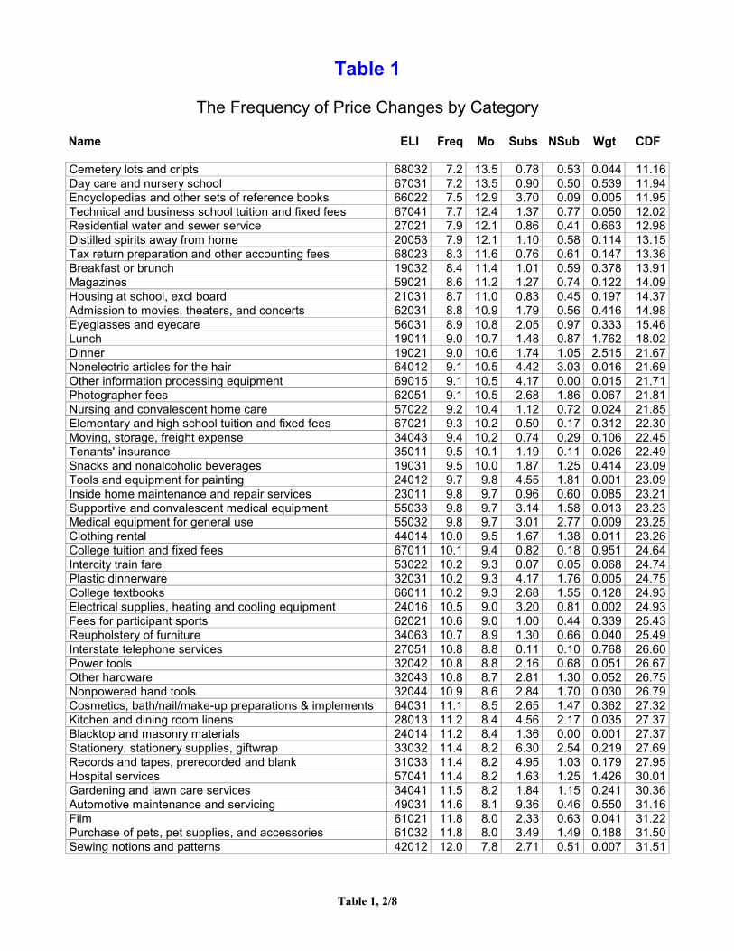
Table 1

The Frequency of Price Changes by Category

Name ELI Freq Mo Subs NSub Wgt CDF

Table 1, 2/8

Cemetery lots and cripts 68032 7.2 13.5 0.78 0.53 0.044 11.16Day care and nursery school 67031 7.2 13.5 0.90 0.50 0.539 11.94Encyclopedias and other sets of reference books 66022 7.5 12.9 3.70 0.09 0.005 11.95Technical and business school tuition and fixed fees 67041 7.7 12.4 1.37 0.77 0.050 12.02Residential water and sewer service 27021 7.9 12.1 0.86 0.41 0.663 12.98Distilled spirits away from home 20053 7.9 12.1 1.10 0.58 0.114 13.15Tax return preparation and other accounting fees 68023 8.3 11.6 0.76 0.61 0.147 13.36Breakfast or brunch 19032 8.4 11.4 1.01 0.59 0.378 13.91Magazines 59021 8.6 11.2 1.27 0.74 0.122 14.09Housing at school, excl board 21031 8.7 11.0 0.83 0.45 0.197 14.37Admission to movies, theaters, and concerts 62031 8.8 10.9 1.79 0.56 0.416 14.98Eyeglasses and eyecare 56031 8.9 10.8 2.05 0.97 0.333 15.46Lunch 19011 9.0 10.7 1.48 0.87 1.762 18.02Dinner 19021 9.0 10.6 1.74 1.05 2.515 21.67Nonelectric articles for the hair 64012 9.1 10.5 4.42 3.03 0.016 21.69Other information processing equipment 69015 9.1 10.5 4.17 0.00 0.015 21.71Photographer fees 62051 9.1 10.5 2.68 1.86 0.067 21.81Nursing and convalescent home care 57022 9.2 10.4 1.12 0.72 0.024 21.85Elementary and high school tuition and fixed fees 67021 9.3 10.2 0.50 0.17 0.312 22.30Moving, storage, freight expense 34043 9.4 10.2 0.74 0.29 0.106 22.45Tenants' insurance 35011 9.5 10.1 1.19 0.11 0.026 22.49Snacks and nonalcoholic beverages 19031 9.5 10.0 1.87 1.25 0.414 23.09Tools and equipment for painting 24012 9.7 9.8 4.55 1.81 0.001 23.09Inside home maintenance and repair services 23011 9.8 9.7 0.96 0.60 0.085 23.21Supportive and convalescent medical equipment 55033 9.8 9.7 3.14 1.58 0.013 23.23Medical equipment for general use 55032 9.8 9.7 3.01 2.77 0.009 23.25Clothing rental 44014 10.0 9.5 1.67 1.38 0.011 23.26College tuition and fixed fees 67011 10.1 9.4 0.82 0.18 0.951 24.64Intercity train fare 53022 10.2 9.3 0.07 0.05 0.068 24.74Plastic dinnerware 32031 10.2 9.3 4.17 1.76 0.005 24.75College textbooks 66011 10.2 9.3 2.68 1.55 0.128 24.93Electrical supplies, heating and cooling equipment 24016 10.5 9.0 3.20 0.81 0.002 24.93Fees for participant sports 62021 10.6 9.0 1.00 0.44 0.339 25.43Reupholstery of furniture 34063 10.7 8.9 1.30 0.66 0.040 25.49Interstate telephone services 27051 10.8 8.8 0.11 0.10 0.768 26.60Power tools 32042 10.8 8.8 2.16 0.68 0.051 26.67Other hardware 32043 10.8 8.7 2.81 1.30 0.052 26.75Nonpowered hand tools 32044 10.9 8.6 2.84 1.70 0.030 26.79Cosmetics, bath/nail/make-up preparations & implements 64031 11.1 8.5 2.65 1.47 0.362 27.32Kitchen and dining room linens 28013 11.2 8.4 4.56 2.17 0.035 27.37Blacktop and masonry materials 24014 11.2 8.4 1.36 0.00 0.001 27.37Stationery, stationery supplies, giftwrap 33032 11.4 8.2 6.30 2.54 0.219 27.69Records and tapes, prerecorded and blank 31033 11.4 8.2 4.95 1.03 0.179 27.95Hospital services 57041 11.4 8.2 1.63 1.25 1.426 30.01Gardening and lawn care services 34041 11.5 8.2 1.84 1.15 0.241 30.36Automotive maintenance and servicing 49031 11.6 8.1 9.36 0.46 0.550 31.16Film 61021 11.8 8.0 2.33 0.63 0.041 31.22Purchase of pets, pet supplies, and accessories 61032 11.8 8.0 3.49 1.49 0.188 31.50Sewing notions and patterns 42012 12.0 7.8 2.71 0.51 0.007 31.51

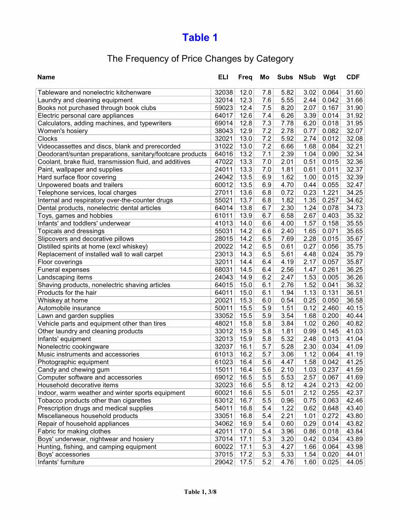
Table 1

The Frequency of Price Changes by Category

Name ELI Freq Mo Subs NSub Wgt CDF

Table 1, 3/8

Tableware and nonelectric kitchenware 32038 12.0 7.8 5.82 3.02 0.064 31.60Laundry and cleaning equipment 32014 12.3 7.6 5.55 2.44 0.042 31.66Books not purchased through book clubs 59023 12.4 7.5 8.20 2.07 0.167 31.90Electric personal care appliances 64017 12.6 7.4 6.26 3.39 0.014 31.92Calculators, adding machines, and typewriters 69014 12.8 7.3 7.78 6.20 0.018 31.95Women's hosiery 38043 12.9 7.2 2.78 0.77 0.082 32.07Clocks 32021 13.0 7.2 5.92 2.74 0.012 32.08Videocassettes and discs, blank and prerecorded 31022 13.0 7.2 6.66 1.68 0.084 32.21Deodorant/suntan preparations, sanitary/footcare products 64016 13.2 7.1 2.39 1.04 0.090 32.34Coolant, brake fluid, transmission fluid, and additives 47022 13.3 7.0 2.01 0.51 0.015 32.36Paint, wallpaper and supplies 24011 13.3 7.0 1.81 0.61 0.011 32.37Hard surface floor covering 24042 13.5 6.9 1.62 1.00 0.015 32.39Unpowered boats and trailers 60012 13.5 6.9 4.70 0.44 0.055 32.47Telephone services, local charges 27011 13.6 6.8 0.72 0.23 1.221 34.25Internal and respiratory over-the-counter drugs 55021 13.7 6.8 1.82 1.35 0.257 34.62Dental products, nonelectric dental articles 64014 13.8 6.7 2.30 1.24 0.078 34.73Toys, games and hobbies 61011 13.9 6.7 6.58 2.67 0.403 35.32Infants' and toddlers' underwear 41013 14.0 6.6 4.00 1.57 0.158 35.55Topicals and dressings 55031 14.2 6.6 2.40 1.65 0.071 35.65Slipcovers and decorative pillows 28015 14.2 6.5 7.69 2.28 0.015 35.67Distilled spirits at home (excl whiskey) 20022 14.2 6.5 0.61 0.27 0.056 35.75Replacement of installed wall to wall carpet 23013 14.3 6.5 5.61 4.48 0.024 35.79Floor coverings 32011 14.4 6.4 4.19 2.17 0.057 35.87Funeral expenses 68031 14.5 6.4 2.56 1.47 0.261 36.25Landscaping items 24043 14.9 6.2 2.47 1.53 0.005 36.26Shaving products, nonelectric shaving articles 64015 15.0 6.1 2.76 1.52 0.041 36.32Products for the hair 64011 15.0 6.1 1.94 1.13 0.131 36.51Whiskey at home 20021 15.3 6.0 0.54 0.25 0.050 36.58Automobile insurance 50011 15.5 5.9 1.51 0.12 2.460 40.15Lawn and garden supplies 33052 15.5 5.9 3.54 1.68 0.200 40.44Vehicle parts and equipment other than tires 48021 15.8 5.8 3.84 1.02 0.260 40.82Other laundry and cleaning products 33012 15.9 5.8 1.81 0.99 0.145 41.03Infants' equipment 32013 15.9 5.8 5.32 2.48 0.013 41.04Nonelectric cookingware 32037 16.1 5.7 5.28 2.30 0.034 41.09Music instruments and accessories 61013 16.2 5.7 3.06 1.12 0.064 41.19Photographic equipment 61023 16.4 5.6 4.47 1.58 0.042 41.25Candy and chewing gum 15011 16.4 5.6 2.10 1.03 0.237 41.59Computer software and accessories 69012 16.5 5.5 5.53 2.57 0.067 41.69Household decorative items 32023 16.6 5.5 8.12 4.24 0.213 42.00Indoor, warm weather and winter sports equipment 60021 16.6 5.5 5.01 2.12 0.255 42.37Tobacco products other than cigarettes 63012 16.7 5.5 0.96 0.75 0.063 42.46Prescription drugs and medical supplies 54011 16.8 5.4 1.22 0.62 0.648 43.40Miscellaneous household products 33051 16.8 5.4 2.21 1.01 0.272 43.80Repair of household appliances 34062 16.9 5.4 0.60 0.29 0.014 43.82Fabric for making clothes 42011 17.0 5.4 3.96 0.86 0.018 43.84Boys' underwear, nightwear and hosiery 37014 17.1 5.3 3.20 0.42 0.034 43.89Hunting, fishing, and camping equipment 60022 17.1 5.3 4.27 1.66 0.064 43.98Boys' accessories 37015 17.2 5.3 5.33 1.54 0.020 44.01Infants' furniture 29042 17.5 5.2 4.76 1.60 0.025 44.05

Table 1

The Frequency of Price Changes by Category

Name ELI Freq Mo Subs NSub Wgt CDF

Table 1, 4/8

Pet food 61031 17.5 5.2 2.13 0.80 0.251 44.41Men's underwear and hosiery 36031 17.6 5.2 2.31 0.40 0.114 44.58Salt and other seasonings and spices 18041 17.6 5.2 1.41 0.64 0.070 44.68Sewing materials for household items 28016 17.7 5.1 2.45 0.71 0.036 44.73Men's nightwear 36032 17.8 5.1 5.37 0.70 0.013 44.75Telephone, peripheral equipment and accessories 69013 17.8 5.1 4.79 3.24 0.065 44.84Books purchased through book clubs 59022 17.9 5.1 7.56 3.12 0.031 44.89Indoor plants and fresh cut flowers 32061 18.0 5.0 4.88 3.07 0.164 45.13Flatware 32033 18.3 4.9 3.91 1.93 0.014 45.15Glassware 32034 18.4 4.9 5.12 2.44 0.014 45.17Automotive brake work 49022 18.5 4.9 9.94 1.25 0.141 45.37Automotive drive train repair 49021 18.5 4.9 9.65 1.13 0.178 45.63Men's accessories 36033 18.7 4.8 4.62 0.78 0.130 45.82Watches 43011 18.8 4.8 5.08 1.32 0.069 45.92Living room tables 29032 18.8 4.8 4.13 2.55 0.063 46.01Portable cool/heat equip., small electric kitchen appliances 32052 19.0 4.8 5.15 2.02 0.078 46.13Soaps and detergents 33011 19.2 4.7 3.16 2.05 0.214 46.44Wine at home 20031 19.3 4.7 3.24 0.84 0.187 46.71Lamps and lighting fixtures 32022 19.4 4.6 6.26 2.61 0.035 46.76Repair to steering, front end, cooling system and A/C 49023 19.5 4.6 10.18 1.26 0.154 46.98Community antenna or cable TV 27031 19.6 4.6 1.91 0.20 0.784 48.12Bicycles 60013 19.6 4.6 6.94 1.10 0.047 48.19Automotive body work 49011 19.7 4.6 10.11 1.45 0.098 48.33Window coverings 32012 19.9 4.5 2.13 0.71 0.038 48.39Other condiments (excl olives, pickles, relishes) 18044 20.1 4.5 0.95 0.51 0.054 48.46Rolls, biscuits, muffins (excl frozen) 2022 20.1 4.5 2.48 1.35 0.135 48.66Intercity bus fare 53021 20.3 4.4 1.31 0.09 0.051 48.73China and other dinnerware 32032 20.4 4.4 5.19 2.34 0.042 48.79Outboard motors and powered sports vehicles 60011 20.5 4.3 6.98 0.96 0.176 49.05Sweet rolls, coffee cake and doughnuts (excl frozen) 2063 20.6 4.3 4.06 2.68 0.073 49.16Canned ham 4032 20.7 4.3 3.45 2.06 0.007 49.17Bedroom furniture other than mattress and springs 29012 20.8 4.3 4.35 2.30 0.193 49.45Occasional furniture 29044 20.9 4.3 4.92 3.25 0.125 49.63Beer, ale, and other alcoholic malt 20011 20.9 4.3 1.03 0.36 0.308 50.07Baby food 18062 20.9 4.3 1.03 0.33 0.088 50.20Cakes and cupcakes (excl frozen) 2041 21.0 4.3 3.49 2.12 0.119 50.37Nondairy cream substitutes 16013 21.0 4.2 1.11 0.57 0.024 50.41Tea 17052 21.0 4.2 1.09 0.53 0.057 50.49Automotive power plant repair 49041 21.1 4.2 10.09 1.75 0.404 51.08Other noncarbonated drinks 17053 21.1 4.2 2.21 0.88 0.069 51.18Lumber, paneling, wall and ceiling tile, awnings, glass 24013 21.6 4.1 1.68 0.67 0.006 51.19Nuts 18032 21.6 4.1 2.28 1.23 0.062 51.28Cigarettes 63011 21.6 4.1 0.35 0.22 0.801 52.44Mattress and springs 29011 21.9 4.1 5.44 2.36 0.146 52.65Smoking accessories 63013 21.9 4.0 3.83 0.00 0.004 52.66Women's underwear 38042 22.1 4.0 3.28 0.77 0.108 52.81Men's footwear 40011 22.2 4.0 4.84 0.79 0.348 53.32Other sweets (excl candy and gum) 15012 22.5 3.9 1.95 1.16 0.075 53.43Admission to sporting events 62032 22.6 3.9 4.80 3.64 0.155 53.65

Table 1

The Frequency of Price Changes by Category

Name ELI Freq Mo Subs NSub Wgt CDF

Table 1, 5/8

Bathroom linens 28011 22.6 3.9 3.40 1.10 0.055 53.73Serving pieces other than silver or glass 32036 22.9 3.9 5.30 3.98 0.005 53.74Sugar and artificial sweeteners 15021 22.9 3.8 1.30 0.70 0.073 53.84Girls' hosiery and accessories 39017 23.0 3.8 7.01 2.17 0.030 53.89Lawn and garden equipment 32041 23.1 3.8 5.92 1.02 0.131 54.08Video game hardware, software and accessories 31023 23.4 3.8 10.15 5.65 0.051 54.15Jewelry 43021 23.4 3.7 4.86 1.76 0.401 54.73Curtains and drapes 28014 24.0 3.6 3.25 1.08 0.057 54.81Kitchen and dining room furniture 29041 24.1 3.6 5.47 3.40 0.163 55.05Cleansing and toilet tissue, paper towels, napkins 33031 24.2 3.6 3.37 2.25 0.208 55.35Girls' footwear 40022 24.2 3.6 7.43 1.27 0.119 55.52Sofas 29021 24.2 3.6 6.73 3.50 0.277 55.93New motorcycles 45031 24.3 3.6 9.30 1.31 0.082 56.04Instant and freeze dried coffee 17032 24.3 3.6 1.17 0.67 0.056 56.13Girls' underwear and nightwear 39016 24.4 3.6 6.80 1.77 0.026 56.16Other processed vegetables 14023 24.6 3.5 2.04 0.40 0.113 56.33Other fuels 25023 24.8 3.5 0.71 0.29 0.014 56.35Canned and dried fruits 13031 24.9 3.5 2.10 0.68 0.068 56.45Noncarbonated fruit flavored drinks 17051 25.0 3.5 2.20 0.92 0.088 56.58Other fats and oils 16012 25.3 3.4 1.16 0.46 0.172 56.83Outdoor equipment 32015 25.3 3.4 8.33 6.19 0.014 56.85Macaroni and cornmeal 1032 25.5 3.4 1.22 0.65 0.094 56.98Cereal 1021 25.5 3.4 1.69 0.87 0.333 57.47Radio, phonographs and taperecorders/players 31031 25.5 3.4 7.80 4.96 0.030 57.51Pies, tarts, turnovers (excl frozen) 2065 25.6 3.4 5.47 2.05 0.044 57.57White bread 2011 25.7 3.4 1.48 0.83 0.124 57.75Truck rental 52052 25.7 3.4 1.60 0.25 0.287 58.17Canned beans other than lima beans 14021 25.8 3.3 1.79 0.37 0.037 58.22Boys' suits, sportcoats, and pants 37016 25.9 3.3 4.82 1.22 0.119 58.40Men's suits 36011 26.0 3.3 3.27 1.03 0.126 58.58Canned and packaged soup 18011 26.3 3.3 1.48 0.69 0.108 58.73Lamb, organ meats, and game 5014 26.4 3.3 1.88 0.82 0.044 58.80Men's pants and shorts 36051 26.4 3.3 3.39 0.84 0.242 59.15Women's accessories 38044 26.4 3.3 11.10 2.02 0.057 59.23Rice 1031 26.5 3.2 1.10 0.58 0.073 59.34Canned or packaged salads and desserts 18061 26.6 3.2 2.12 1.05 0.079 59.45Living room chairs 29031 26.7 3.2 7.05 3.17 0.136 59.65Infants' and toddlers' sleepwear 41014 26.9 3.2 7.37 1.42 0.014 59.67Other dairy products 10012 26.9 3.2 1.48 0.58 0.077 59.78Bedroom linens 28012 27.0 3.2 5.02 1.60 0.170 60.03Prepared Flour Mixes 1012 27.1 3.2 2.14 0.85 0.043 60.09Other frozen fruits and fruit juices 13012 27.1 3.2 1.28 0.55 0.025 60.13Canned fish or seafood 7011 27.4 3.1 1.80 0.75 0.058 60.21Sauces and gravies 18043 27.6 3.1 1.01 0.55 0.134 60.41Margarine 16011 27.9 3.1 1.48 0.39 0.043 60.47Bologna, liverwurst, salami 5012 28.0 3.0 2.02 1.22 0.085 60.59Ship fares 53023 28.0 3.0 4.78 1.10 0.101 60.74Women's footwear 40031 28.0 3.0 6.80 1.62 0.424 61.35Other canned or packaged foods 18063 28.1 3.0 1.80 0.76 0.223 61.68

Table 1

The Frequency of Price Changes by Category

Name ELI Freq Mo Subs NSub Wgt CDF

Table 1, 6/8

Olives, pickles, relishes 18042 28.1 3.0 1.50 0.71 0.035 61.73Dryers 30022 28.5 3.0 5.43 0.21 0.042 61.79Automobile finance charges 51011 28.6 3.0 1.84 0.04 0.493 62.50Lunchmeats 5013 28.7 3.0 2.79 1.08 0.150 62.72Microwave ovens 30032 29.0 2.9 8.16 1.39 0.030 62.77Potato chips and other snacks 18031 29.1 2.9 2.62 1.57 0.212 63.07Boys' footwear 40021 29.7 2.8 9.51 1.26 0.094 63.21Bread other than white 2021 29.7 2.8 2.07 1.27 0.137 63.41Outdoor furniture 29043 29.8 2.8 9.88 4.63 0.040 63.47Window air conditioners 30034 29.9 2.8 7.22 2.00 0.039 63.52Men's sportcoats and tailored jackets 36012 30.1 2.8 4.47 1.39 0.030 63.57Frozen bakery products 2064 30.3 2.8 2.68 1.22 0.076 63.68Tires 48011 30.5 2.7 2.72 0.58 0.290 64.10Men's coats and jackets 36013 30.9 2.7 8.28 2.51 0.116 64.27Frozen vegetables 14011 31.0 2.7 1.95 0.79 0.099 64.41Peanut butter 16014 31.0 2.7 1.10 0.48 0.040 64.47Televisions 31011 31.0 2.7 9.03 3.61 0.269 64.86Floor covering equipment and sewing machines 32051 31.1 2.7 7.45 1.56 0.060 64.94Video cassette recorders, disc players, cameras 31021 31.2 2.7 10.70 4.09 0.095 65.08Portable dishwashers 30033 31.2 2.7 3.65 2.50 0.002 65.08Ice cream and related products 10041 31.4 2.7 1.96 0.96 0.178 65.34Bread and cracker products 2062 31.5 2.6 1.99 1.99 0.014 65.36Women's pants and shorts 38033 31.5 2.6 7.71 2.44 0.345 65.86Other fresh milk and cream 9021 31.6 2.6 1.08 0.22 0.222 66.19Flour 1011 31.7 2.6 0.75 0.38 0.029 66.23Bottled or tank gas 25021 31.7 2.6 0.69 0.38 0.055 66.31Canned cut corn 14022 31.9 2.6 0.91 0.29 0.023 66.34Luggage 42013 31.9 2.6 6.21 2.62 0.034 66.39Carbonated drinks other than cola 17012 32.4 2.6 1.99 0.91 0.146 66.60Motor oil 47021 32.7 2.5 1.00 0.33 0.045 66.67Men's shirts 36041 32.7 2.5 6.20 1.55 0.270 67.06Cheese 10021 32.9 2.5 1.82 0.85 0.307 67.50Stoves and ovens excluding microwave ovens 30031 33.0 2.5 7.45 1.09 0.037 67.56Girls' skirts and pants 39014 33.2 2.5 10.10 3.28 0.076 67.67Refrigerators and home freezers 30011 33.5 2.5 7.14 0.85 0.106 67.82Cookies 2042 33.7 2.4 2.27 1.51 0.157 68.05Fresh, canned, or bottled fruit juices 13013 33.7 2.4 2.28 1.03 0.210 68.35Playground equipment 61012 33.8 2.4 12.07 8.25 0.007 68.36Components and other sound equipment 31032 34.1 2.4 9.25 5.42 0.132 68.56Frozen orange juice 13011 34.4 2.4 0.95 0.43 0.030 68.60Fresh whole milk 9011 34.4 2.4 0.79 0.12 0.201 68.89Washers 30021 35.4 2.3 6.80 0.65 0.057 68.97Other poultry 6031 36.0 2.2 5.38 0.96 0.129 69.16Frankfurters 5011 36.1 2.2 2.22 0.92 0.077 69.27Boys' shirts 37013 36.2 2.2 10.17 3.24 0.063 69.36Infants' and toddlers' play and dresswear 41012 36.3 2.2 14.68 4.60 0.049 69.43Other beef 3043 36.4 2.2 0.94 0.75 0.053 69.51Frozen prepared foods other than meals 18022 36.5 2.2 2.24 1.15 0.158 69.74Shellfish (excl canned) 7021 37.0 2.2 2.39 1.22 0.124 69.92

Table 1

The Frequency of Price Changes by Category

Name ELI Freq Mo Subs NSub Wgt CDF

Table 1, 7/8

Roasted coffee 17031 37.1 2.2 1.36 0.68 0.103 70.07Frozen prepared meals 18021 37.4 2.1 3.53 1.72 0.072 70.17New trucks 45021 37.7 2.1 10.80 9.04 1.953 73.01Men's active sportswear 36035 37.8 2.1 10.80 2.14 0.061 73.10Pork sausage 4042 37.9 2.1 1.40 0.63 0.077 73.21Lodging while out of town 21021 38.1 2.1 1.80 0.52 1.571 75.49Personal computers and peripheral equipment 69011 38.4 2.1 16.12 7.79 0.488 76.19Infants' and toddlers' outerwear 41011 38.6 2.1 19.32 7.70 0.011 76.21Cola drinks 17011 38.8 2.0 0.91 0.42 0.306 76.66New cars 45011 39.1 2.0 10.26 8.11 2.747 80.64Women's coats and jackets 38011 39.2 2.0 14.86 6.93 0.155 80.87Fresh whole chicken 6011 39.4 2.0 2.12 0.14 0.088 80.99Women's nightwear 38041 40.6 1.9 15.50 3.04 0.088 81.12Fresh or frozen chicken parts 6021 40.7 1.9 1.39 0.38 0.273 81.52Apples 11011 41.4 1.9 0.18 0.04 0.102 81.67Other roast (excl chuck and round) 3041 42.2 1.8 0.93 0.75 0.050 81.74Fish (excl canned) 7022 42.4 1.8 2.55 1.42 0.167 81.98Crackers 2061 42.5 1.8 1.53 0.91 0.075 82.09Girls' tops 39013 42.7 1.8 17.00 5.47 0.070 82.19Women's skirts 38032 42.9 1.8 16.69 7.81 0.071 82.30Bananas 11021 43.0 1.8 0.07 0.03 0.106 82.45Electricity 26011 43.4 1.8 0.64 0.08 2.884 86.63Bacon 4011 43.5 1.7 1.51 0.74 0.071 86.74Girls' active sportswear 39015 43.6 1.7 18.93 5.51 0.033 86.78Girls' coats and jackets 39011 43.8 1.7 19.43 6.02 0.023 86.82Women's active sportswear 38034 44.6 1.7 17.26 3.43 0.092 86.95Women's tops 38031 45.0 1.7 17.94 6.93 0.471 87.63Men's sweaters 36034 45.3 1.7 13.53 4.85 0.046 87.70Butter 10011 45.5 1.6 0.90 0.24 0.042 87.76Boys' coats and jackets 37011 45.7 1.6 15.27 5.81 0.024 87.80Ground beef 3011 46.1 1.6 0.67 0.32 0.288 88.21Boys' active sportswear 37017 46.6 1.6 19.12 3.96 0.027 88.25Pork roast, picnics, other pork 4041 46.8 1.6 1.44 0.75 0.131 88.44Other steak (excl round and sirloin) 3042 46.8 1.6 0.72 0.53 0.156 88.67Diesel 47017 47.2 1.6 0.70 0.03 0.254 89.04Potatoes 12011 47.3 1.6 0.41 0.13 0.098 89.18Women's suits 38051 47.3 1.6 19.45 8.45 0.123 89.36Pork chops 4021 47.9 1.5 0.35 0.19 0.138 89.56Round steak 3051 48.2 1.5 0.62 0.46 0.060 89.65Sirloin steak 3061 48.4 1.5 0.65 0.48 0.084 89.77Boys' sweaters 37012 48.4 1.5 17.18 5.47 0.007 89.78Women's dresses 38021 48.5 1.5 25.44 11.08 0.296 90.21Ham (excl canned) 4031 50.4 1.4 4.00 2.03 0.118 90.38Fuel oil 25011 52.5 1.3 0.40 0.18 0.169 90.63Other fresh vegetables 12041 52.8 1.3 0.17 0.07 0.250 90.99Round roast 3031 53.1 1.3 0.48 0.40 0.045 91.05Chuck roast 3021 54.3 1.3 0.76 0.65 0.043 91.12Oranges 11031 54.7 1.3 0.45 0.11 0.057 91.20Girls' dresses and suits 39012 55.1 1.2 28.49 12.80 0.045 91.26

Table 1

The Frequency of Price Changes by Category

Name ELI Freq Mo Subs NSub Wgt CDF

Table 1, 8/8

Automobile rental 52051 56.8 1.2 2.86 0.40 0.758 92.36Other fresh fruits 11041 59.7 1.1 0.24 0.08 0.247 92.72Other motor fuel 47018 61.8 1.0 4.46 1.80 0.032 92.77Eggs 8011 61.8 1.0 0.64 0.26 0.107 92.92Lettuce 12021 62.4 1.0 0.06 0.05 0.064 93.02Utility natural gas service 26021 64.2 1.0 0.34 0.08 1.012 94.48Airline fares 53011 69.1 0.9 0.45 0.25 0.829 95.69Tomatoes 12031 71.0 0.8 0.22 0.03 0.078 95.80Premium unleaded gasoline 47016 76.2 0.7 2.81 0.89 0.998 97.25Mid-grade unleaded gasoline 47015 77.5 0.7 2.55 0.82 0.865 98.50Regular unleaded gasoline 47014 78.9 0.6 2.56 0.83 1.031 100.00

ELI = Entry Level Item in the CPI (around 4-5 items priced each month in each geographic area).

Freq = the estimated average monthly frequency of price changes over 1995-1997 (� in the text).

Mo = the mean duration between price changes implied by � [= -1/ln(1-�)].

Subs = the average item substitution rate in the ELI over 1995-1997.

NSub = the average noncomparable item substitution rate in the ELI over 1995-1997.

Wgt = Share of the ELI in the 1995 Consumer Expenditure Survey (these sum to 68.9).

CDF = cumulative distribution function of Freq within the share of the CPI covered.

All data are from the U.S. Department of Labor.

Table 2

Table 2

Monthly Frequency of Price Changes By Year, 1995 to 2002

Year Median Frequency Median Duration

1995 21.3 % 4.2 months

1996 20.8 4.3

1997 19.9 4.5

1998 20.7 4.3

1999 22.4 3.9

2000 24.0 3.6

2001-02 23.1 3.8

Notes: The medians are across 350 expenditure-weighted categories (ELIs). 2001-02refers to the 15-month period from January 2001 through March 2002.

Data Source: U.S. Department of Labor, Commodities and Services Substitution RateTable, various years.

Table 3

Table 3

Monthly Frequency of Price Changes for Selected Categories

% of Price Quoteswith Price Changes

% of Price Quoteswith Price Changes Net ofthe Item Substitution %

All goods and services 26.1 (1.0) 22.7 (1.0)

Durable Goods 29.8 (2.5) 21.5 (2.5)Nondurable Goods 29.9 (1.5) 26.6 (1.5)

Services 20.7 (1.5) 19.1 (1.5)

Food 25.3 (1.9) 23.7 (1.9)Home Furnishings 26.4 (1.8) 23.7 (1.8)

Apparel 29.2 (3.0) 20.2 (3.0)Transportation 39.4 (1.8) 34.2 (1.8)Medical Care 9.4 (3.2) 8.2 (3.2)Entertainment 11.3 (3.5) 8.2 (3.5)

Other 11.0 (3.3) 9.9 (3.3)

Raw Goods 54.3 (1.9) 52.9 (1.7)Processed Goods 20.5 (0.8) 16.7 (0.7)

Notes: Frequencies are weighted means of category components. Standard errors are inparentheses. Durables, Nondurables and Services coincide with U.S. National Incomeand Product Account classifications. Housing (reduced to home furnishings in our data),apparel, transportation, medical care, entertainment, and other are BLS ExpenditureClasses for the CPI. Raw goods include gasoline, motor oil and coolants, fuel oil andother fuels, electricity, natural gas, meats, fish, eggs, fresh fruits, fresh vegetables, andfresh milk and cream.

Data Source: U.S. Department of Labor (1997).

Table 4

Table 4

Predicting Price Changes Across Goods

Dependent Variable = Frequency of Price Changes across ELIs

Regressors�

(A) (B) (C) (D)

4-firm Concentration Ratio -0.30 (0.05)

-0.30 (0.04)

-0.002 (0.04)

Wholesale Markup -1.20 (0.12)

-0.10 (0.13)

Noncomparable Substitution Rate 1.25 (0.33)

2.17 (0.26)

2.86(0.29)

Raw Good 34.1(2.7)

37.7(1.8)

Adjusted R2 0.15 0.36 0.63 0.56

Number of goods (ELIs) 231 221 221 350

Notes: Each regression is weighted by the importance of the ELI in 1995 ConsumerExpenditures. Standard errors are in parentheses.

Table 5

Table 5

Aggregate and Sectoral Inflation Rates (Short Sample)

Variable�

(A)Monthly Inflation

(B)Monthly Growth ofReal Consumption

Aggregate of 123 Sectors

� 0.20 (0.13) �0.32 (0.12)x

��0.22 0.57

Across i = 1, ..., 123 sectors

Mean �i �0.05 (0.02)x �0.08 (0.03)x

Mean ��,i 0.83 (0.08) 1.66 (0.17)

Correlation between �i and �i 0.26 (0.09) �0.56 (0.08)x

Correlation between ��,i and �i 0.68 (0.07) 0.45 (0.08)

Notes:

Define dxt = first difference of xt , where xt is the log of the price or real consumption.

For the aggregate: dxt = � dxt-1 + �t , where �t is i.i.d. with standard deviation ��.

For sector i: dxi,t = �i dxi,t-1 + �i,t , where �i,t is i.i.d. with standard deviation ��,i.

The sample is 1995:M1 to 2000:M6. The 123 sectors represent 63.3% of 1995 Consumer Expenditures,and each sector is weighted by its expenditure share. Standard errors are in parentheses.

Table 6

Table 6

Aggregate and Sectoral Inflation Rates (Longer Sample)

Variable�

(A)Monthly Inflation

(B)Monthly Growth ofReal Consumption

Aggregate of 123 Sectors

� 0.63 (0.03) �0.14 (0.04)x

��0.22 0.79

Across i = 1, ..., 123 sectors

Mean �i 0.26 (0.02) �0.11 (0.02)x

Mean ��,i 0.91 (0.07) 2.43 (0.19)

Correlation between �i and �i �0.06 (0.09)x �0.40 (0.08)x

Correlation between ��,i and �i 0.52 (0.08) 0.35 (0.08)

Notes:

Define dxt = first difference of xt , where xt is the log of the price or real consumption.

For the aggregate: dxt = � dxt-1 + �t , where �t is i.i.d. with standard deviation ��.

For sector i: dxi,t = �i dxi,t-1 + �i,t , where �i,t is i.i.d. with standard deviation ��,i.

The sample is 1959:M1 to 2000:M6. The 123 sectors represent 63.3% of 1995 Consumer Expenditures, andeach sector is weighted by its expenditure share. Standard errors are in parentheses.

Table 7

Table 7

Observed Inflation for Flexible-Price and Sticky-Price Goods

From 1995-2000 data(A) (B)

From 1959-2000 data(C) (D)

Variable�

Price Inflation Growth of RealConsumption

Price Inflation Growth of RealConsumption

Flexible-price good

� 0.01 �0.34x 0.24 �0.22x

��1.54 2.63 1.37 3.29

Sticky-price good

� �0.11x 0.15 0.28 �0.02x

��0.19 0.78 0.50 1.65

Flexible versus sticky

�flexible � �sticky 0.12 (0.04) �0.49 (0.07)x �0.04 (0.05)x �0.21 (0.04)x

��, flexible � ��, sticky 1.35 (0.13) 1.85 (0.33) 0.87 (0.13) 1.63 (0.40)

Notes:

Define dxit = first difference of xit , where xit is the log of the price or real consumption.

dxi,t = �i dxi,t-1 + �i,t , where �i,t is i.i.d. with S.D. ��,i .

�flexible and ��, flexible refer to the serial correlation and volatility fitted for a good with monthly frequencyof price changes of 48.5% (the 90th percentile of frequency in Table 1); �sticky and ��, sticky refer to thosefitted for a good with monthly frequency of price changes of 6.5% (the 10th percentile).

Table 8

Table 8

Inflation from a Staggered Pricing Model

Only Aggregate Shocks

(A) (B)

Aggregate and Sector Shocks

(C) (D)Variable

� Price Inflation Growth of RealConsumption

Price Inflation Growth of RealConsumption

Flexible-price good

� 0.48 (0.03) �0.30 (0.04)x 0.47 (0.03) 0.16 (0.04)

��0.68 (0.02) 0.67 (0.02) 1.01 (0.04) 1.08 (0.04)

Sticky-price good

� 0.91 (0.02) 0.01 (0.05) 0.90 (0.02) 0.10 (0.05)

��0.11 (0.01) 0.86 (0.03) 0.17 (0.01) 0.91 (0.03)

Notes:

dxit = first difference of xit , where xit is the log of the price or real consumption.

dxi,t = �i dxi,t-1 + �i,t , where �i,t is i.i.d. with S.D. ��,i and �i = S.D.( dxi,t) = [��,i2/(1-� i

2)]½.

�flexible and ��, flexible refer to the serial correlation and volatility predicted by the staggered-pricing modelfor a good with monthly frequency of price changes of 1/2 (near the 90th percentile of frequency in Table1); �sticky and ��, sticky refer to those predicted by the model for a good with monthly frequency of pricechanges of 1/15 (near the 10th percentile).

0

5

10

15

20

25

30

0.0 12.5 25.0 37.5 50.0 62.5 75.0

Figure 1

Num

ber o

f Con

sum

ptio

n C

ateg

orie

s

Monthly Frequency of Price Changes over 1995-1997

0 5 10 15 20 25-0.2

0

0.2

0.4

0.6

0.8

1

1.2

Figure 2

% responses to a 1% money supply shock (persistence of money growth is �m = 0)

CL

0 5 10 15 20 25-0.2

0

0.2

0.4

0.6

0.8

1

1.2CfCs

0 5 10 15 20 250

0.2

0.4

0.6

0.8

1

1.2

1.4

Months (flexible = fixed for 2 months, sticky = fixed for 15 months)

PfPs

0 5 10 15 20 25-1

-0.5

0

0.5

1

1.5

Figure 3

% responses to a 1% productivity shock (persistence is �a = 1)

CL

0 5 10 15 20 250

0.2

0.4

0.6

0.8

1

1.2

1.4CfCs

0 5 10 15 20 25-1.4

-1.2

-1

-0.8

-0.6

-0.4

-0.2

0

Months (flexible = fixed for 2 months, sticky = fixed for 15 months)

PfPs

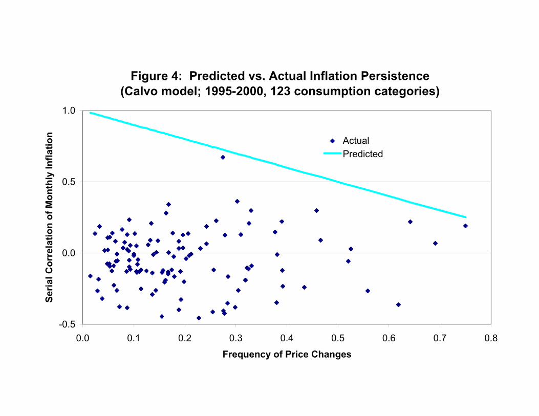
Figure 4: Predicted vs. Actual Inflation Persistence(Calvo model; 1995-2000, 123 consumption categories)

-0.5

0.0

0.5

1.0

0.0 0.1 0.2 0.3 0.4 0.5 0.6 0.7 0.8Frequency of Price Changes

Seria

l Cor

rela

tion

of M

onth

ly In

flatio

n ActualPredicted

Figure 5: Predicted vs. Actual Inflation Persistence(Calvo model; 1959-2000, 123 consumption categories)

-0.5

0.0

0.5

1.0

0.0 0.1 0.2 0.3 0.4 0.5 0.6 0.7 0.8Frequency of Price Changes

Seria

l Cor

rela

tion

of M

onth

ly In

flatio

n ActualPredicted

Figure 6: Marginal Cost Needed to Generate Sectoral Inflation (Calvo model; 1995-2000 data for 123 categories)

-0.4

-0.2

0.0

0.2

0.4

0.6

0.8

1.0

1 10 100 1000 10000

Standard Error of Innovations to Marginal Cost (in %)

Seria

l Cor

rela

tion

of M

argi

nal C

ost Sticky third

Middle third Flexible third Mean process in the data Two s.d.s from the mean

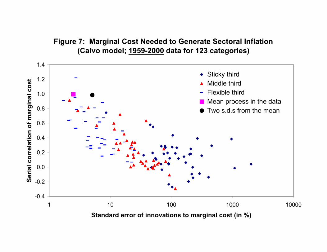
Figure 7: Marginal Cost Needed to Generate Sectoral Inflation(Calvo model; 1959-2000 data for 123 categories)

-0.4

-0.2

0.0

0.2

0.4

0.6

0.8

1.0

1.2

1.4

1 10 100 1000 10000

Standard error of innovations to marginal cost (in %)

Seria

l cor

rela

tion

of m

argi

nal c

ost Sticky third

Middle third Flexible third Mean process in the data Two s.d.s from the mean

31

References

Aoki, Kosuke (2001), "Optimal Monetary Policy Responses to Relative Price Changes,"Journal of Monetary Economics, 48, 55-80.

Ball, Lawrence and David Romer (1991), "Sticky Prices as Coordination Failure," AmericanEconomic Review, 81, 539-552.

Barro, Robert J. (1972), "A Theory of Monopolistic Price Adjustment," Review of EconomicStudies.

Basu, Susanto and John G. Fernald (1997), "Returns to Scale in U.S. Production: Estimatesand Implications," 105, 249-283.Journal of Political Economy

Benigno, Pierpaolo, "Optimal Monetary Policy in a Currency Area," manuscript, New YorkUniversity.

Bils, Mark (1987), "The Cyclical Behavior of Marginal Cost and Price," AmericanEconomic Review 77, 838-855.

Blinder, Alan S., Elie R. D. Canetti, David E. Lebow, and Jeremy B. Rudd (1998), AskingAbout Prices: A New Approach to Understanding Price Stickiness, Russell SageFoundation, New York.

Boskin Commission Report (1996), "Toward a More Accurate Measure of the Cost ofLiving," final report to the Senate Finance Committee from the Advisory Commission toStudy the Consumer Price Index, http://www.ssa.gov/history/reports/boskinrpt.html.

Calvo, Guillermo A. (1983), "Staggered Pricing in a Utility Maximizing Framework,"Journal of Monetary Economics 12, 383-398.

Caplin and Spulber (1987), "Menu Costs and the Neutrality of Money," Quarterly Journalof Economics 102, 703-726.

Carlton, Dennis W. (1986), "The Rigidity of Prices," 76, 637-American Economic Review658.

Carlton, Dennis W. (1989) "The Theory and The Facts of How Markets Clear: Is IndustrialOrganization Valuable for Understanding Macroeconomics?" in Handbook of IndustrialOrganization, eds. Schmalensee and Willig, Elsevier, New York.

Caucutt, Elizabeth M., Mrinal Gosh, and Christina M.L. Kelton (1999), "Durability VersusConcentration as an Explanation for Price Inflexibility," Review of IndustrialOrganization 14, 27-50.

32

Cecchetti, Stephen G. (1986), "The Frequency of Price Adjustment: A Study of theNewsstand Prices of Magazines," 31, 255-274.Journal of Econometrics

Chari, V.V., Patrick J. Kehoe, and Ellen R. McGrattan (2000), "Sticky Price Models of theBusiness Cycle: Can the Contract Multiplier Solve the Persistence Problem?"Econometrica 68, 1151-1179.

valier, Judith A., Anil K. Kashyap, and Peter E. Rossi (2000), "Why Don't Prices RiseCheDuring Periods of Peak Demand? Evidence from Scanner Data," NBER Working Paper7981.

Christiano Lawrence J., Martin Eichenbaum, and Charles L. Evans (1999), "Monetary PolicyShocks: What Have We Learned and to What End?" chapter 2 in Handbook ofMacroeconomics, John B. Taylor and Michael Woodford, eds., Elsevier, New York.

Clarida, Richard, Jordi Gali, and Mark Gertler (1999), "The Science of Monetary Policy,"Journal of Economic Literature 37, 1661-1707.

Dotsey, Michael and Robert G. King (2001), "Pricing, Production, and Persistence," NBERWorking Paper 8407.

Erceg, Christopher J., Dale W. Henderson, and Andrew T. Levin (2000), "Optimal MonetaryPolicy with Staggered Wage and Price Contracts," 46,Journal of Monetary Economics281-313.

Fuhrer, Jeffrey C. and George R. Moore (1995), "Inflation Persistence," Quarterly Journalof Economics 110, 127-159.

Gali, Jordi (1999), "Technology, Employment, and the Business Cycle: Do TechnologyShocks Explain Aggregate Fluctuations?" 89, 249-271.American Economic Review

Gali, Jordi and Mark Gertler (1999), "Inflation Dynamics: A Structural EconometricAnalysis," 44, 195-222.Journal of Monetary Economics

Goodfriend, Marvin and Robert G. King (1997) "The New Keynsian Neoclassical Synthesisand the Role of Monetary Policy," NBER Macroeconomics Annual 12, 233-283.

Hall, Simon, Mark Walsh, and Anthony Yates (2000), "Are UK Companies' Prices Sticky?",Oxford Economic Papers 52 (3), 425-446.

Hawkes, William J. and Frank W. Piotrowski (2000), "Using Scanner Data to Improve theQuality of Measurement and the Measurement of Quality in the Consumer Price Index," inScanner Data and Price Indexes, Robert Feenstra and Matthew Shapiro, editors,forthcoming, University of Chicago Press.

33

Kackmeister, Alan (2001), "Has Retail Price Behavior Changed Since 1889? Evidence fromMicrodata," manuscript, University of California, Berkeley.

Kashyap, Anil K. (1995), "Sticky Prices: New Evidence from Retail Catalogs", QuarterlyJournal of Economics 110, 245-274.

King, Robert G. and Charles Plosser (1984), "Money, Credit, and Prices in a Real BusinessCycle," 74, 363-380.American Economic Review

Levy, Daniel, Mark Bergen, Shantanu Dutta, and Robert Venable (1997), "The Magnitude ofMenu Costs: Direct Evidence from Large U.S. Supermarket Chains," Quarterly Journalof Economics 112 (3), 791-823.

MacDonald, James N. and Daniel Aaronson (2001), "How Do Retail Prices React toMinimum Wage Increases?" manuscript, U.S. Department of Agriculture.

Ohanian, Lee, Alan C. Stockman, and L. Kilian (1995), "The Effects of Real and MonetaryShocks in a Business Cycle Model with Some Sticky Prices, Journal of Money, Credit,and Banking, 27.

Pashigian, B. Peter (1988), "Demand Uncertainty and Sales: A Study of Fashion andMarkdown Pricing," 78 (5), 936-953.American Economic Review

Rotemberg, Julio J. (1996), "Prices, Output, and Hours: An Empirical Analysis Based on aSticky-Price Model," 37, 505-533.Journal of Monetary Economics

Rotemberg, Julio J. and Michael Woodford (1997), "An Optimization-based EconometricFramework for the Evaluation of Monetary Policy," NBER Macroeconomics Annual 12,297-346.

Sbordone, Argia (2002), "Prices and Unit Labor Costs: A New Test of Price Stickiness,"Journal of Monetary Economics 49(2), pp. 265-292.

Sims, Chris (2001), "Rational Inattention," manuscript, Princeton University.

Taylor, John B. (1999), "Staggered Price and Wage Setting in Macroeconomics," chapter 15in Handbook of Macroeconomics, John B. Taylor and Michael Woodford, eds., Elsevier,New York.

U.S. Department of Labor (1997), BLS Handbook of Methods, Bulletin 2490, U.S.Government Printing Office.

Willis, Jonathan L. (2000), "Estimation of Adjustment Costs in a Model of State-DependentPricing" Federal Reserve Bank of Kansas City Research Working Paper 00-07, December.