NBER WORKING PAPER SERIES

OPTIMAL DEFAULTS AND ACTIVE DECISIONS

James J. ChoiDavid Laibson

Brigitte C. MadrianAndrew Metrick

Working Paper 11074http://www.nber.org/papers/w11074

NATIONAL BUREAU OF ECONOMIC RESEARCH1050 Massachusetts Avenue

Cambridge, MA 02138January 2005

We thank Hewitt Associates for their help in providing the data. We are particularly grateful to Lori Lucas,Jim McGhee, Scott Peterson, Deborah Bonus and Yan Xu, some of our many contacts at Hewitt. We alsoappreciate many helpful conversations with Harlan Fleece and the exceptional research assistance of NelsonUhan, Jared Gross, John Friedman, Hongyi Li, Laura Serban, Keith Ericson, Ben Grossman, and Fuad Faridi.Richard Thaler, Mark Iwry, Shlomo Benartzi, Annamaria Lusardi and seminar participants at the Universityof Chicago, Harvard, MIT, Berkeley, Cornell, USC, LSE, Wharton, Dartmouth, Stanford, the New YorkFederal Reserve, the Russell Sage Foundation and the NBER have provided much useful feedback. Choiacknowledges financial support from a National Science Foundation Graduate Research Fellowship and theMustard Seed Foundation. Choi, Laibson, and Madrian acknowledge individual and collective financialsupport from the National Institute on Aging (grants R01-AG-16605, R29-AG-013020, and T32-AG00186).Laibson also acknowledges financial support from the Sloan Foundation. The views expressed herein arethose of the author(s) and do not necessarily reflect the views of the National Bureau of Economic Research.

© 2005 by James J. Choi, David Laibson, Brigitte C. Madrian, and Andrew Metrick. All rights reserved.Short sections of text, not to exceed two paragraphs, may be quoted without explicit permission providedthat full credit, including © notice, is given to the source.

Optimal Defaults and Active DecisionsJames J. Choi, David Laibson, Brigitte C. Madrian, and Andrew MetrickNBER Working Paper No. 11074January 2005JEL No. D0, E21, G23

ABSTRACT

Defaults can have a dramatic influence on consumer decisions. We identify an overlooked but

practical alternative to defaults: requiring individuals to make an explicit choice for themselves. We

study such "active decisions" in the context of 401(k) saving. We find that compelling new hires to

make active decisions about 401(k) enrollment raises the initial fraction that enroll by 28 percentage

points relative to a standard opt-in enrollment procedure, producing a savings distribution three

months after hire that would take three years to achieve under standard enrollment. We also present

a model of 401(k) enrollment and derive conditions under which the optimal enrollment regime is

automatic enrollment (i.e., default enrollment), standard enrollment (i.e., default non-enrollment),

or active decisions (i.e., no default and compulsory choice). Active decisions are optimal when

consumers have a strong propensity to procrastinate and savings preferences are highly hetergeneous.

Naive beliefs about future time-inconsistency strengthen the normative appeal of the active decision

enrollment regime.

James J. ChoiDepartment of EconomicsHarvard UniversityCambridge, MA 02138jjchoi@nber.org

David LaibsonDepartment of EconomicsLittauer M-14Harvard UniversityCambridge, MA 02138and NBERdlaibson@harvard.edu

Brigitte C. MadrianDepartment of Business and Public PolicyUniversity of Pennsylvania Wharton School3620 Locust Walk, Suite 1400 SH-DHPhiladelphia, PA 19104-6372and NBERbmadrian@wharton.upenn.edu

Andrew MetrickThe Wharton SchoolUniversity of Pennsylvania3620 Locust WalkPhiladelphia, PA 19104and NBERmetrick@wharton.upenn.edu

Economists have studied two kinds of 401(k) enrollment. Under �standard enrollment,�

employees are by default not enrolled and can choose to opt into the plan. Under �automatic

enrollment,�employees are by default enrolled and can choose to opt out. In this paper, we

analyze an overlooked third alternative: requiring employees to make an explicit choice for

themselves. In this �active decision�regime there is no default to fall back on.

Ex ante, it might seem that a default should not matter if agents believe it is arbitrarily

chosen and if opting out of the default is easy. In practice, defaults� even bad defaults�

tend to be sticky; employees rarely opt out.1 This perverse property of defaults has been

documented in a wide range of settings: organ donation decisions (Johnson and Goldstein

2003, Abadie and Gay 2004), car insurance plan choices (Johnson et al 1993), car option pur-

chases (Park, Yun, and MacInnis 2000), and consent to receive e-mail marketing (Johnson,

Bellman, and Lohse 2003).

In light of this inertia, defaults are socially desirable when agents have a shared optimum

and the default leads them to it (e.g., a low-fee index fund). But even a well-chosen default

may be undesirable if agents have heterogeneous needs.2 For example, in a �rm whose

workforce includes young, cash-strapped single parents and older employees who need to

quickly build a retirement nest egg, one 401(k) savings rate isn�t right for everyone.

Active decisions are an intriguing, though imperfect, alternative to defaults. On the

positive side, an active decision mechanism avoids the biases introduced by defaults because it

does not corral agents into a single default choice. The active decision mechanism encourages

agents to think about an important decision and thereby avoid procrastinating. On the

negative side, an active decision compels agents to struggle with a potentially time-consuming

decision� which they may not be quali�ed to make� and then explicitly express their choice.

Some people would welcome a benign third party who is willing to make and automatically

implement that decision for them. In addition, social engineers might prefer a default that

aggressively encourages some social goal, like organ donation or retirement saving.3

1For example, about three-quarters of 401(k) participants in �rms with automatic enrollment retainboth the default contribution rate and the default asset allocation (Madrian and Shea 2001, Choi et al2002, 2004). These �choices� are puzzling because most companies with automatic enrollment have veryconservative defaults; a typical �rm might have a default contribution rate of 2% of income, even thoughcontributions up to 6% of income garner matching contributions from the employer.

2One could design defaults that are tailored to each employee, but these would be construed as advicein the current regulatory environment. Firms are not allowed to give �nancial advice to their employees,although they are allowed to give employees access to an independent �nancial advisor.

3See Hurst (2004) and Warshawsky and Ameriks (2000) for evidence that many U.S. households are

3

The current paper lays the groundwork for a debate about active decisions by describing

how an active decision 401(k) enrollment regime worked at one large �rm. In addition,

we present a model that provides a formal framework for evaluating the relative e¢ cacy of

di¤erent choice mechanisms, including defaults and active decisions.

Our empirical study exploits a natural experiment in 401(k) enrollment. One large �rm

(unintentionally) used active decisions and then switched to a standard enrollment regime.

This change in 401(k) enrollment procedures occurred as a by-product of the transition from

a paper-and-pencil administrative system to a phone-based administrative system. The

�rm did not anticipate that the transition to a phone-based system with a default of non-

enrollment would transform the psychology of 401(k) participation. Rather, the change in

administrative systems was motivated solely by the convenience and e¢ ciency of phone-

based enrollment. The loss of active decision e¤ects was a collateral consequence of that

transition.

We �nd that active decisions raise the initial fraction of employees enrolled by 28 percent-

age points relative to what is obtained with a standard default of non-enrollment. Active

decisions raise average savings rates and accumulated balances by accelerating decision-

making. We show that conditional on demographics, each employee under active decisions

will on average immediately choose a savings rate similar to what she would otherwise take

up to three years to attain under standard enrollment. There is also no evidence that em-

ployees make more haphazard savings choices under active decisions. Because the typical

worker will change jobs several times before retirement, accelerating the 401(k) savings de-

cision by three years at the beginning of each job transition can have a large impact on

accumulated wealth at retirement.

In our model of the enrollment process, defaults matter for three key reasons. First,

employees face a cost of opting out of the employer�s chosen default. Second, this cost varies

over time, creating option value to waiting for a low-cost period to take action. Third,

employees with present-biased preferences may procrastinate in their decision to opt out of

the default. We derive conditions under which the optimal enrollment regime is automatic

enrollment, standard enrollment, or active decisions. Active decisions are socially optimal

undersaving. However, this is an open question with research on both sides of the debate. See Aguiarand Hurst (2004) and Engen, Gale, and Uccello (1999) for evidence that the lifecycle model with liquidityconstraints matches U.S. data.

4

when consumers have highly heterogeneous savings preferences and a strong propensity to

procrastinate.

The rest of this paper proceeds as follows. Section 1 describes the details of the two

401(k) enrollment regimes at the company we study. Section 2 describes our data. Section

3 compares the 401(k) savings decisions of employees hired under the active decision regime

to those hired under the standard enrollment regime. Section 4 then models the enrollment

decision of a time-inconsistent employee who has rational expectations, derives the socially

optimal enrollment mechanism for such agents, and also considers the case of employees

with naive expectations about their future time inconsistency. Section 5 discusses the key

implications of the model. Section 6 concludes and brie�y discusses practical considerations

in the implementation of active decision mechanisms.

1 The Natural Experiment

We use employee-level data from a large, publicly-traded Fortune 500 company in the

�nancial services industry. In December 1999, this �rm had o¢ ces in all 50 states, as well

as the District of Columbia and Puerto Rico. This paper will consider the 401(k) savings

decisions of employees at the �rm from January 1997 through December 2001.

Until November 1997, all newly hired employees at the �rm were required to submit a form

within 30 days of their hire date stating their 401(k) participation preferences, regardless of

whether they wished to enroll or not. Although there was no tangible penalty for not

returning the 401(k) form, human resource o¢ cers report that only 5% of employees failed

to do so.4 We believe that this high compliance rate arose because the form was part of a

packet that included other forms whose submission was legally required (e.g., employment

eligibility veri�cation forms, tax withholding forms, other bene�ts enrollment forms, etc.).

Moreover, employees who did not return the form were reminded to do so by the human

resources department.

Employees who declined to participate in the 401(k) plan during this initial enrollment

period could not subsequently enroll in the plan until the beginning (January 1) of succeeding

calendar years. Later in the paper, we will show that this delay played no role in the active

decision e¤ect.

4A failure to return the form was treated as a negative 401(k) election.

5

At the beginning of November 1997, the company switched from a paper-based 401(k)

enrollment system to a telephone-based system. Employees hired after this change no longer

received a 401(k) enrollment form when hired. Instead, they were given a toll-free phone

number to call if and when they wished to enroll in the 401(k) plan. We call this new

system the �standard enrollment�regime because its non-enrollment default is used by most

companies. The telephone-based system also allowed employees to enroll on a daily basis,

rather than only at the beginning of each calendar year as had previously been the case.

This change applied not only to employees hired after November 1997, but to all employees

working at the company.

A number of other 401(k) plan features also changed at the same time. We believe that

these additional changes made 401(k) participation more attractive, so our estimates of the

active decision e¤ect are a lower bound on the true e¤ect. These other changes include

a switch from monthly to daily account valuation, the introduction of 401(k) loans, the

addition of two new funds as well as employer stock to the 401(k) investment portfolio,5 and

a switch from annual to quarterly 401(k) statements. Table 1 summarizes the 401(k) plan

rules before and after the November 1997 changes.

2 The Data

We have two types of employee data. The �rst dataset is a series of cross-sections at

year-ends 1998, 1999, 2000, and 2001. Each cross-section contains demographic information

for everybody employed by the company at the time, including birth date, hire date, gender,

marital status, state of residence, and salary. For 401(k) plan participants, each cross-section

also contains the date of enrollment and year-end information on balances, asset allocation,

and the terms of any outstanding 401(k) loans. The second dataset is a longitudinal history

of every individual transaction in the plan from September 1997 through April 2002: savings

rate elections, asset allocation elections for contributions, trades among funds, loan-based

withdrawals and repayments, �nancial hardship withdrawals, retirement withdrawals, and

rollovers.

To analyze the impact of active decisions, we compare the behavior of two employee

5Prior to November 1997, employer stock was available as an investment option only for after-taxcontributions.

6

groups: employees hired between January 1, 1997 and July 31, 1997 under the active decision

regime,6 and employees hired between January 1, 1998 and July 31, 1998 under the standard

enrollment regime.7 We refer to the �rst group as the �active decision cohort�and the second

group as the �standard enrollment cohort.�

The active decision cohort is �rst observed in our cross-sectional data in December 1998,

18 to 24 months after hire, and in the longitudinal data starting in September 1997, 3 to 9

months after hire. The longitudinal data only contain participants. The standard enrollment

cohort is also observed in our cross-sectional data starting in December 1998, but this is only

6 to 12 months after their hire date. In the longitudinal data, 401(k) participants from this

cohort are observed as soon as they enroll.

Since 401(k) participants are less likely to subsequently leave their employer,8 our data

structure introduces selection e¤ects that are stronger for the active decision cohort than

the standard enrollment cohort. To equalize the sample selectivity of the active decision

and standard enrollment cohorts, we restrict the standard enrollment cohort sample to those

employees who were still employed by the company in December 1999. We have no reason

to believe that the turnover rates of employees from these two cohorts were di¤erent over

these time horizons. The economic environment faced by these two groups of employees

was similar until the start of the 2001 recession. In addition, company o¢ cials reported no

material changes in hiring or employment practices during this period.

Table 2 presents demographic statistics on the active decision and standard enrollment

cohorts at the end of December in the year after they were hired. The cohorts are similar in

age, gender composition, income, and geographical distribution. The dimension along which

they di¤er most is marital status, and even here the di¤erences are not large: 57.2% of the

active decision cohort is married, while this is true for only 52.2% of the standard enrollment

cohort. The third column of Table 2 shows that the new-hire cohorts are di¤erent from

6We exclude employees hired prior to January 1, 1997 because the company made two substantive planchanges that took e¤ect January 1, 1997. First, the company eliminated a one-year service requirement for401(k) eligibility. Second, the company changed the structure of its 401(k) match. Although active decisionswere used until the end of October 1997, we do not include employees hired from August through Octoberto avoid any confounds produced by the transition to standard enrollment. For example, an enrollmentblackout was implemented for several weeks during the transition.

7For both groups, we restrict our sample to employees under age 65 who are eligible to participate in theplan.

8See Even and MacPherson (1999).

7

employees at the company overall. As expected, the new-hire cohorts are younger, less likely

to be married, and paid less on average. The last column reports statistics from the Current

Population Survey, providing a comparison between the company�s employees and the total

U.S. workforce. The company has a relatively high fraction of female employees, probably

because it is in the service sector. Employees at the company also have relatively high

salaries. This is partially due to the fact that the company does not employ a representative

fraction of very young employees, who are more likely to work part-time and at lower wages.

3 Empirical Results

3.1 401(k) Enrollment

We �rst examine the impact of the active decisions on enrollment in the 401(k). Figure 1

plots the fraction enrolled in the 401(k) after three months of tenure for employees who were

hired in the �rst seven months of 1997 (the active decision cohort) and the �rst seven months

of 1998 (the standard enrollment cohort). We use the third month of tenure because it could

take up to three months for enrollments to be processed in the active decision regime.9 The

average three-month enrollment rate is 69% for the active decision cohort, versus 41% for

the standard enrollment cohort, and this di¤erence is statistically signi�cant at the 99% level

for every hire month.

Figure 2 plots the fraction of employees who have enrolled in the 401(k) plan against

tenure. The active decision cohort�s enrollment fraction grows more slowly than the stan-

dard enrollment cohort�s, so the enrollment gap decreases with tenure. Nonetheless, the

active decision cohort�s enrollment fraction exceeds the standard enrollment cohort�s by 17

percentage points at 24 months of tenure, and by 5 percentage points at 42 months. These

di¤erences are statistically signi�cant at the 99% level for every tenure level.

Figures 1 and 2 could be misleading if enrollees under the active decision regime are

subsequently more likely to stop contributing to the 401(k) plan. However, attrition rates

from the 401(k) plan are indistinguishable under the active decision regime and the standard

9Enrollments were only processed on the �rst of each month under the active decision regime. Sinceemployees had 30 days to turn in their form, an employee who was hired late in a month and turned in herform just before the deadline could be enrolled three months after her hire.

8

enrollment regime. Indeed, 401(k) participation is a nearly-absorbing state under either

enrollment regime.10

We ascribe the active decision e¤ect to the fact that active decision employees had to

express their 401(k) participation decision during their �rst month of employment, rather

than being able to delay action inde�nitely. However, there is another distinction between

the active decision and standard enrollment regimes as implemented at the company. Under

the standard enrollment regime, employees could enroll in the 401(k) plan at any time.

Under the active decision regime, if employees did not enroll in the plan in their �rst 30

days at the company, their next enrollment opportunity did not come until January 1 of

the following calendar year.11 Therefore, in addition to the required a¢ rmative or negative

enrollment decision, the active decision cohort faced a narrower enrollment window than the

standard enrollment cohort. In theory, this limited enrollment window could cause higher

initial 401(k) enrollment rates by accelerating the enrollment of employees who would have

otherwise enrolled between the third month of their tenure and the following January.

However, the enrollment di¤erences between the cohorts are too large to be explained

by a window e¤ect. If only a window e¤ect were operative, enrollment fractions for the two

groups should be equal after twelve months of tenure. In fact, the enrollment fraction of the

active decision cohort at three months of tenure is not matched by the standard enrollment

cohort until it approaches three years of tenure.

There is also no evidence that the window e¤ect can even partially explain the active

decision e¤ect. If the window e¤ect were important, then enrollment during the initial 30-

day eligibility period under active decisions should be higher for employees hired earlier in

the year than employees hired later in the same year, since employees hired earlier have a

longer wait until the next January 1 enrollment opportunity. We �nd no such relationship;

instead, the correlation between the three-month enrollment fraction and the time from hire

month to the following January 1 is negative (�0:20). This result is corroborated in datafrom pre-1997 cohorts hired under the active decision regime.

Although active decisions induce earlier 401(k) enrollment, this may come at the cost

10These calculations are available from the authors.11In fact, the active decision cohort we analyze (January to June 1997 hires) was able to enroll in the

401(k) plan any time after November 1997, when the company switched to the phone-based daily enrollmentsystem. At hire, however, the active decision employees were not aware of this impending change and wouldhave believed January 1, 1998 to be their next enrollment opportunity.

9

of more careful and deliberate thinking about how much to save for retirement. We now

turn our focus to other 401(k) savings outcomes to see what impact active decisions have on

them.

3.2 401(k) Contribution Rate

Figure 3 plots the relationship between tenure and the average 401(k) contribution rate

for both the active decision and standard enrollment cohorts. The averages include both

participants (who have a non-zero contribution rate) and non-participants (who have a zero

contribution rate). Because our longitudinal data do not start until September 1997, the

contribution rate pro�le cannot be computed for the entire active decision cohort until 9

months of tenure.

The active decision cohort contributes 4.8% of income on average at month 9, and this

slowly increases to 5.5% of income by the fourth year of employment. In contrast, the

standard enrollment cohort contributes only 3.6% of income on average at month 9, and it

takes three years for it to match the active decision cohort�s nine-month savings rate. At

each tenure level in the graph, the di¤erence between the groups�average contribution rates

is statistically signi�cant at the 99% level.

Figure 4 plots the average contribution rate of employees who have a non-zero contribu-

tion rate (i.e., 401(k) participants). In contrast to Figure 3, active decision participants have

a lower average contribution rate than standard enrollment participants until the fourth year

of tenure.12 To gain insight into this pattern, we plot the 25th, 50th, 75th, and 90th per-

centile contribution rates for the standard enrollment and active decision cohorts in Figure

5. Non-participants are assigned a zero contribution rate and are included in these distrib-

utions. We see that at each of these points in the distribution, the active decision cohort�s

contribution rate matches or exceeds the standard enrollment cohort�s contribution rate at

virtually every tenure level. There is nearly no gap between the two cohorts�contribution

rates at the 90th percentile, where enrollment in the 401(k) occurs immediately for both

groups. As we move down the savings distribution, the di¤erence between the two cohorts

tends to increase, and most of this di¤erence is due to active decision cohort employees

12These di¤erences are statistically di¤erent at the 99% level through the 29th month of tenure, and atthe 95% level through the 30th month of tenure.

10

signing up for the 401(k) plan earlier in their tenure. Overall, it seems that employees save

at roughly the same rate under both regimes once they have enrolled. Therefore, the lower

average contribution rate among active decision participants is not due to active decisions

lowering the savings rates of those who would have otherwise contributed more under stan-

dard enrollment. Rather, active decisions bring employees with weaker savings motives into

the participant pool earlier in their tenure.

Table 3 presents the results of a regression of the two regimes� contribution rates on

demographic variables. Both active decision and standard enrollment employees are included

in the regression, regardless of participation status. If the employee was hired under the

standard enrollment regime, the dependent variable is equal to the contribution rate at 36

months after hire. If the employee was hired under the active decision regime, the dependent

variable is equal to an estimate of the contribution rate at 3 months after hire. This estimate

is constructed by taking the earliest available contribution rate (which may be as late as 9

months after hire) for the active decision employee and setting that contribution rate to

zero if the employee had not enrolled in the plan within 3 months of hire. The explanatory

variables are a constant, marital status, log of salary, and age dummies. The e¤ect of these

variables is allowed to vary between the active decision and standard enrollment cohorts.13

The regression coe¢ cients suggest that in expectation, there is little di¤erence between

the savings rate an employee chooses immediately after hire under active decisions and the

rate she would have in e¤ective three years after hire under standard enrollment. The only

variable we can statistically reject having the same e¤ect under both regimes is marital

status; active decisions seem to eliminate the savings gap between married and single indi-

viduals. Furthermore, there is no evidence that savings choices under active decisions are

more haphazard than savings rates under standard enrollment; a Goldfeld-Quandt test can-

not reject the null hypothesis that the regression residuals for the two cohorts were drawn

from distributions with the same variances.14 If the active decision deadline causes people

to make more mistakes when choosing their savings rate, then these mistakes are almost

perfectly predicted by their demographics.

In sum, active decisions cause employees to immediately choose a savings rate that they

13The number of data points in the regression is less than the total number of employees in the two cohortsbecause some employees are missing demographic data.14The ratio of the mean squared error for the standard enrollment cohort to the mean squared error for

the active decision cohort is 1.018.

11

would otherwise take up to three years to attain under standard enrollment.

3.3 401(k) Asset Allocation

The e¤ect of active decisions on asset allocation cannot be cleanly inferred because the

menu of investment fund options changed in November 1997, the same time that the company

switched from active decisions to the standard enrollment regime. Prior to the change,

employer stock was only available as an investment option for after-tax contributions, which

are rare because they are generally less tax-e¢ cient than pre-tax contributions.15 During the

transition to standard enrollment, employer stock was added as an investment option for pre-

tax 401(k) contributions. Subsequently, the average allocation to employer stock more than

doubled and the average allocation to all other asset classes correspondingly decreased. It is

impossible to determine how much of this increase was caused by the standard enrollment

regime, and how much was caused by the ten-fold increase in the fraction of employees for

whom employer stock was a viable investment option.

The impact of active decisions on asset allocation is an important open question, since

employees have low levels of �nancial knowledge about di¤erent asset classes (John Hancock

2002) and tend to make poor asset allocation choices (Benartzi and Thaler 2001, Cronqvist

and Thaler 2004). In section 4, we explain why active decisions are likely to be better suited

for contribution rate choices than for asset allocation choices. We believe asset allocation

decisions are best treated with a clear default option.

3.4 401(k) Asset Accumulation

We next consider the impact of active decisions on asset accumulation. Asset accumula-

tion analysis is confounded by time e¤ects, since asset returns are highly volatile. Moreover,

the investment fund menu changed over time, as explained above, further confounding this

analysis. Nonetheless, it is the level of asset accumulation that will ultimately drive re-

tirement timing and consumption levels. Studying asset accumulation also gives us insight

15Pre-tax contributions are more tax-e¢ cient unless the contributor has a short investment horizon andexpects tax rates to rise sharply in the future. At the company, 12% of 401(k) participants made after-tax contributions during 1998. Participants who make after-tax contributions tend to be at their pre-taxcontribution limit.

12

into whether increased 401(k) loan activity o¤sets increased contribution rates under active

decisions.16

To measure asset accumulation, we divide 401(k) balances by annual base pay. Our mea-

sure of 401(k) balances excludes outstanding principal from 401(k) loans and any balances

an employee rolled over from a previous employer.

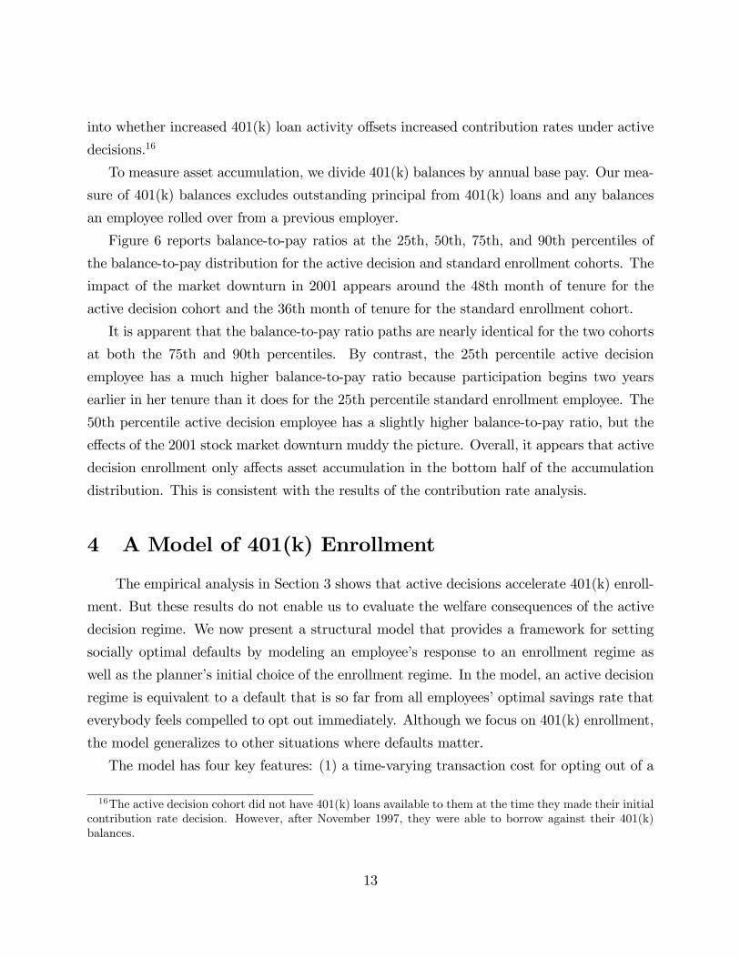
Figure 6 reports balance-to-pay ratios at the 25th, 50th, 75th, and 90th percentiles of

the balance-to-pay distribution for the active decision and standard enrollment cohorts. The

impact of the market downturn in 2001 appears around the 48th month of tenure for the

active decision cohort and the 36th month of tenure for the standard enrollment cohort.

It is apparent that the balance-to-pay ratio paths are nearly identical for the two cohorts

at both the 75th and 90th percentiles. By contrast, the 25th percentile active decision

employee has a much higher balance-to-pay ratio because participation begins two years

earlier in her tenure than it does for the 25th percentile standard enrollment employee. The

50th percentile active decision employee has a slightly higher balance-to-pay ratio, but the

e¤ects of the 2001 stock market downturn muddy the picture. Overall, it appears that active

decision enrollment only a¤ects asset accumulation in the bottom half of the accumulation

distribution. This is consistent with the results of the contribution rate analysis.

4 A Model of 401(k) Enrollment

The empirical analysis in Section 3 shows that active decisions accelerate 401(k) enroll-

ment. But these results do not enable us to evaluate the welfare consequences of the active

decision regime. We now present a structural model that provides a framework for setting

socially optimal defaults by modeling an employee�s response to an enrollment regime as

well as the planner�s initial choice of the enrollment regime. In the model, an active decision

regime is equivalent to a default that is so far from all employees�optimal savings rate that

everybody feels compelled to opt out immediately. Although we focus on 401(k) enrollment,

the model generalizes to other situations where defaults matter.

The model has four key features: (1) a time-varying transaction cost for opting out of a

16The active decision cohort did not have 401(k) loans available to them at the time they made their initialcontribution rate decision. However, after November 1997, they were able to borrow against their 401(k)balances.

13

default, which creates an option value for delaying action and generates inertia at a default;

(2) present-bias, which generates self-defeating procrastination and exacerbates this inertia;

(3) heterogeneity in optimal savings rates across workers, which implies that a single default

will not be optimal for all workers; and (4) asymmetric information of the form where each

worker knows more than the planner about the worker�s optimal savings rate.

The third and fourth assumptions are critical for our welfare results. If the planner

knows the worker�s true optimum, then the planner should simply set that optimum as the

default, saving the worker the time and e¤ort of making the choice for himself. There is a

growing body of evidence that planners make better asset allocation choices than workers

(Benartzi and Thaler 2001, Cronqvist and Thaler 2004). However, survey evidence suggests

that workers have idiosyncratic savings needs, and that workers understand this individual

variation (Choi et al 2004). Hence, the model that follows is best thought of as a model

of saving rates choices and not of asset allocation choices. For asset allocation choices,

well-chosen defaults are likely to dominate active decisions.

Our model has two stages. First, a benign planner creates an enrollment mechanism (a

default or active decision). Then, individual workers make a sequence of savings decisions.

Our analysis solves the model through backwards induction. We begin by solving the worker�s

problem, holding �xed the enrollment mechanism. Then we solve the planner�s problem by

identifying the enrollment mechanism that maximizes social surplus.

4.1 The Sophisticated Worker�s Problem

Workers have quasi-hyperbolic preferences, so they have the discount function 1; ��; ��2; :::

where 0 < � � 1 (Phelps and Pollak 1968, Laibson 1997). Workers su¤er from a dynamic

inconsistency problem; they have impatient preferences for the present but patient prefer-

ences for the future. For simplicity, we set � = 1, eliminating long-run discounting. We begin

by assuming that workers are sophisticated and understand their dynamically inconsistent

preferences. Unlike naive agents, whose actions we characterize later, sophisticated actors

make current decisions based on rational expectations of future actions.

Each worker has an exogenously determined optimal savings rate s that is known to the

worker but not observed by the planner.17 The planner only knows the probability density

17For simplicity, we assume that each worker�s optimal savings rate is constant over time.

14

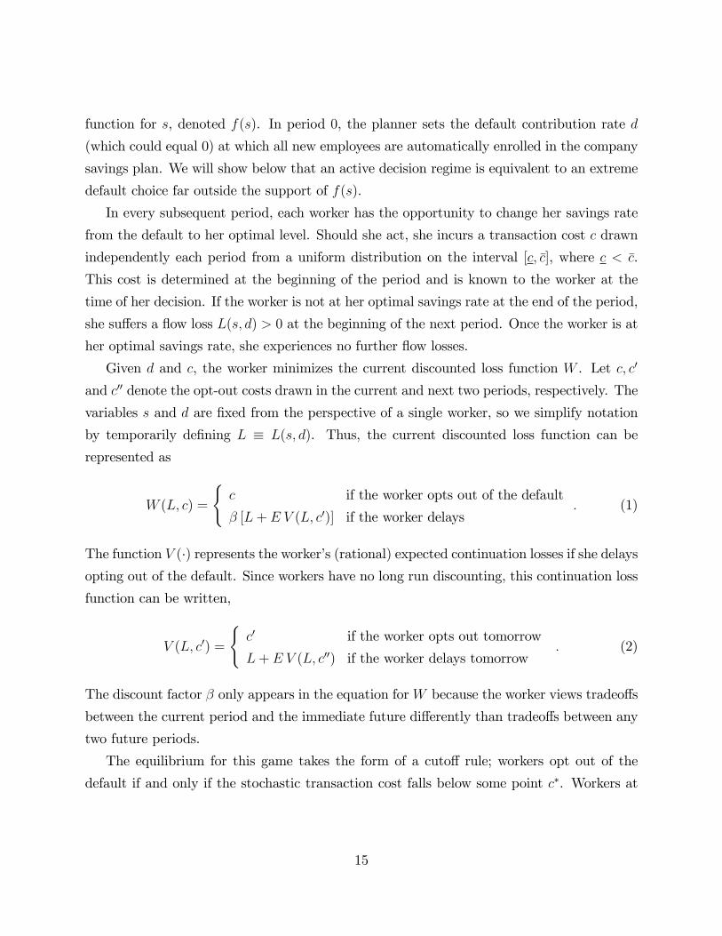
function for s, denoted f(s). In period 0, the planner sets the default contribution rate d

(which could equal 0) at which all new employees are automatically enrolled in the company

savings plan. We will show below that an active decision regime is equivalent to an extreme

default choice far outside the support of f(s).

In every subsequent period, each worker has the opportunity to change her savings rate

from the default to her optimal level. Should she act, she incurs a transaction cost c drawn

independently each period from a uniform distribution on the interval [c; �c], where c < �c.

This cost is determined at the beginning of the period and is known to the worker at the

time of her decision. If the worker is not at her optimal savings rate at the end of the period,

she su¤ers a �ow loss L(s; d) > 0 at the beginning of the next period. Once the worker is at

her optimal savings rate, she experiences no further �ow losses.

Given d and c, the worker minimizes the current discounted loss function W . Let c; c0

and c00 denote the opt-out costs drawn in the current and next two periods, respectively. The

variables s and d are �xed from the perspective of a single worker, so we simplify notation

by temporarily de�ning L � L(s; d). Thus, the current discounted loss function can be

represented as

W (L; c) =

(c if the worker opts out of the default

� [L+ E V (L; c0)] if the worker delays: (1)

The function V (�) represents the worker�s (rational) expected continuation losses if she delaysopting out of the default. Since workers have no long run discounting, this continuation loss

function can be written,

V (L; c0) =

(c0 if the worker opts out tomorrow

L+ E V (L; c00) if the worker delays tomorrow: (2)

The discount factor � only appears in the equation forW because the worker views tradeo¤s

between the current period and the immediate future di¤erently than tradeo¤s between any

two future periods.

The equilibrium for this game takes the form of a cuto¤ rule; workers opt out of the

default if and only if the stochastic transaction cost falls below some point c�. Workers at

15

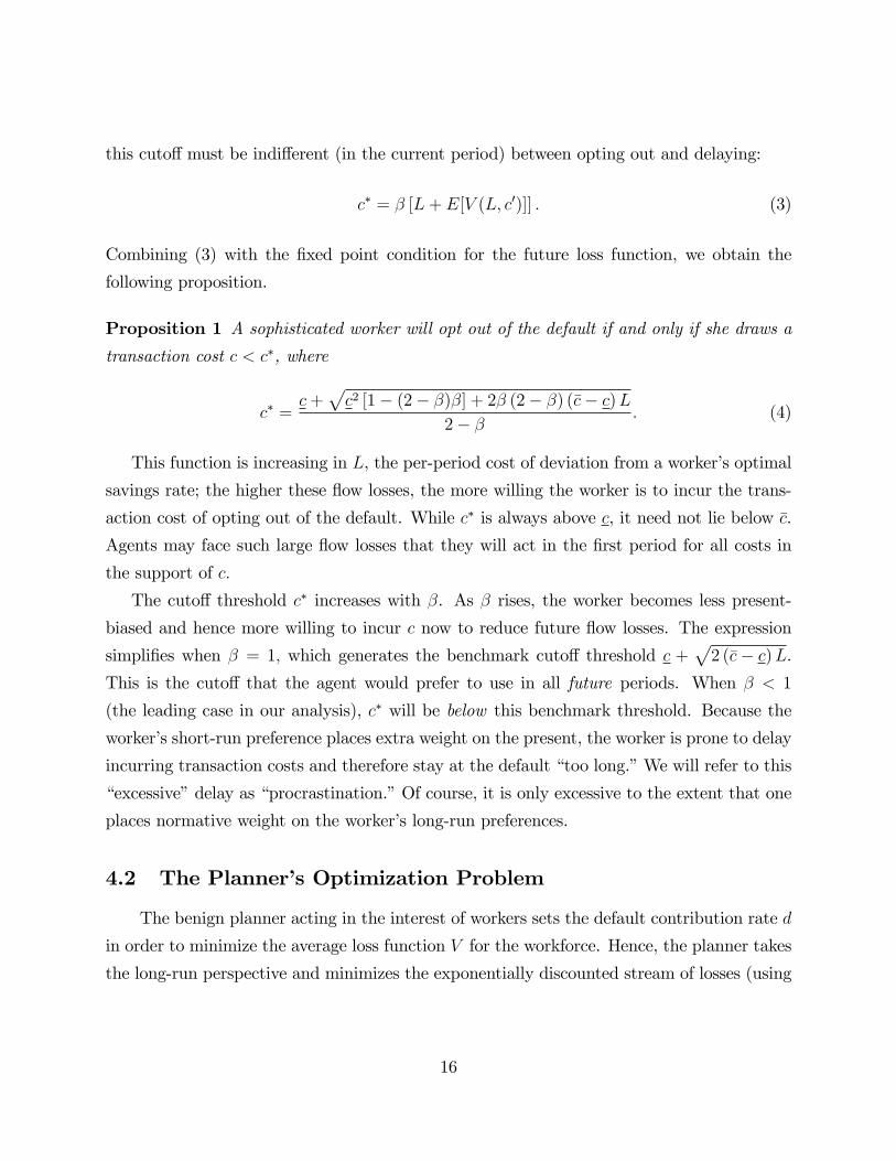
this cuto¤ must be indi¤erent (in the current period) between opting out and delaying:

c� = � [L+ E[V (L; c0)]] : (3)

Combining (3) with the �xed point condition for the future loss function, we obtain the

following proposition.

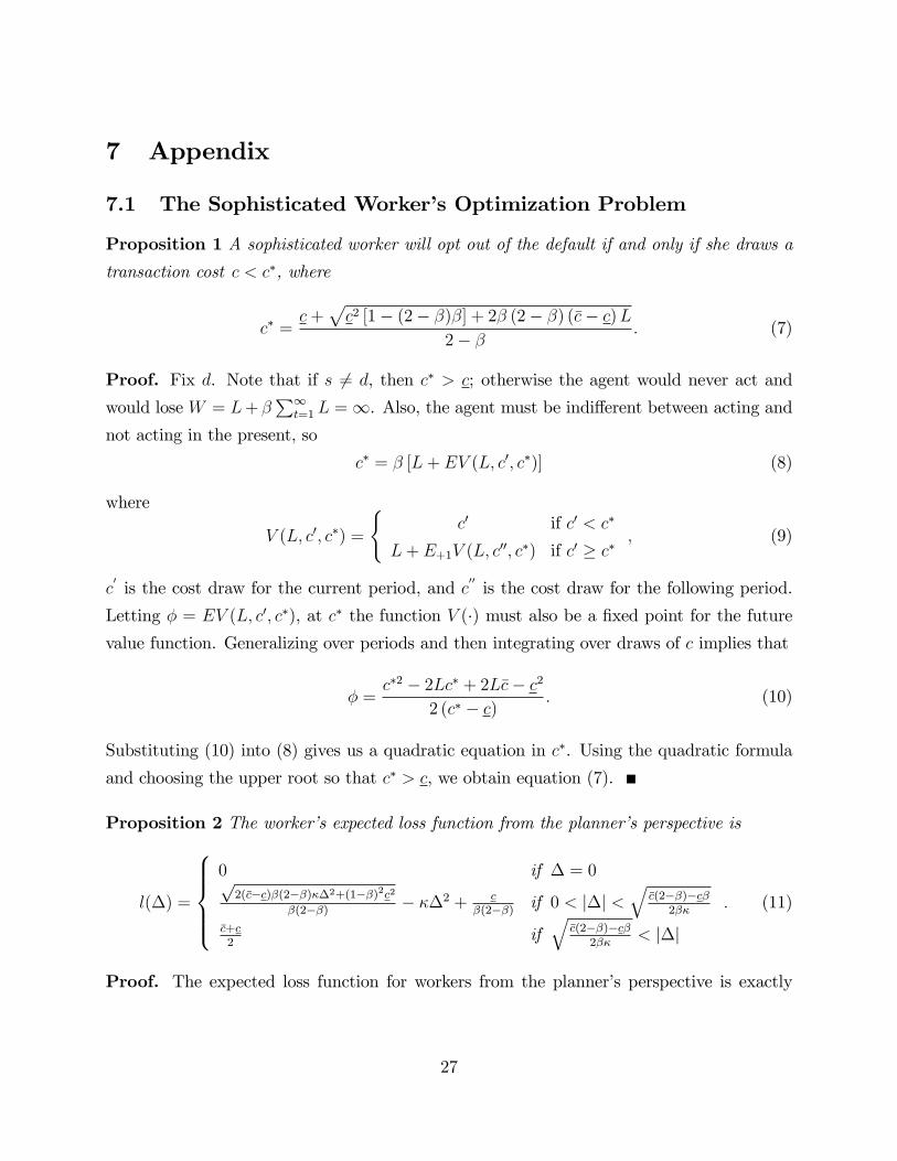
Proposition 1 A sophisticated worker will opt out of the default if and only if she draws a

transaction cost c < c�, where

c� =c+

pc2 [1� (2� �)�] + 2� (2� �) (�c� c)L

2� � : (4)

This function is increasing in L, the per-period cost of deviation from a worker�s optimal

savings rate; the higher these �ow losses, the more willing the worker is to incur the trans-

action cost of opting out of the default. While c� is always above c, it need not lie below �c.

Agents may face such large �ow losses that they will act in the �rst period for all costs in

the support of c:

The cuto¤ threshold c� increases with �. As � rises, the worker becomes less present-

biased and hence more willing to incur c now to reduce future �ow losses. The expression

simpli�es when � = 1; which generates the benchmark cuto¤ threshold c +p2 (�c� c)L.

This is the cuto¤ that the agent would prefer to use in all future periods. When � < 1

(the leading case in our analysis), c� will be below this benchmark threshold. Because the

worker�s short-run preference places extra weight on the present, the worker is prone to delay

incurring transaction costs and therefore stay at the default �too long.�We will refer to this

�excessive�delay as �procrastination.�Of course, it is only excessive to the extent that one

places normative weight on the worker�s long-run preferences.

4.2 The Planner�s Optimization Problem

The benign planner acting in the interest of workers sets the default contribution rate d

in order to minimize the average loss function V for the workforce. Hence, the planner takes

the long-run perspective and minimizes the exponentially discounted stream of losses (using

16

the exponential discount factor � = 1).18

The planner�s decision problem takes the form

d� = argmind

Zl(s; d)f(s)ds;

where l(s; d) is the expected value of a worker�s loss function (integrating over the distribution

of current opt-out costs):

l(s; d) � EcV (L(s; d); c):

Alternatively, we can write l(s; d) using the Bellman Equation:

l(s; d) =

(E(cjc � c�) with probability F (c�)

L(s; d) + l(s; d) with probability 1� F (c�):

For analytical tractability, we assume L(s; d) = �(s� d)2.19 This functional form allows

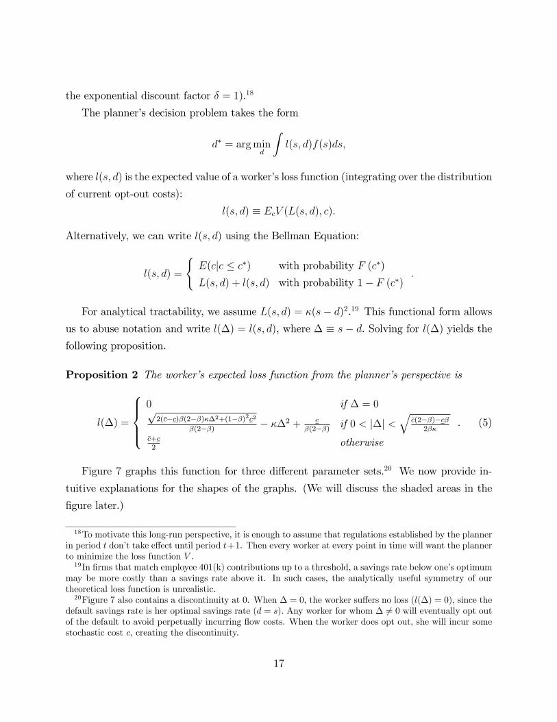
us to abuse notation and write l(�) = l(s; d), where � � s� d. Solving for l(�) yields thefollowing proposition.

Proposition 2 The worker�s expected loss function from the planner�s perspective is

l(�) =

8>><>>:0 if � = 0p2(�c�c)�(2��)��2+(1��)2c2

�(2��) � ��2 + c�(2��) if 0 < j�j <

q�c(2��)�c�

2��

�c+c2

otherwise

: (5)

Figure 7 graphs this function for three di¤erent parameter sets.20 We now provide in-

tuitive explanations for the shapes of the graphs. (We will discuss the shaded areas in the

�gure later.)

18To motivate this long-run perspective, it is enough to assume that regulations established by the plannerin period t don�t take e¤ect until period t+1. Then every worker at every point in time will want the plannerto minimize the loss function V .19In �rms that match employee 401(k) contributions up to a threshold, a savings rate below one�s optimum

may be more costly than a savings rate above it. In such cases, the analytically useful symmetry of ourtheoretical loss function is unrealistic.20Figure 7 also contains a discontinuity at 0. When � = 0, the worker su¤ers no loss (l(�) = 0), since the

default savings rate is her optimal savings rate (d = s): Any worker for whom � 6= 0 will eventually opt outof the default to avoid perpetually incurring �ow costs. When the worker does opt out, she will incur somestochastic cost c, creating the discontinuity.

17

When j�j is in a neighborhood of zero, increasing j�j increases expected losses becausethe worker is moved further from her optimal savings rate. These losses plateau at the left

and right boundaries of each panel in Figure 7 because above a certain value of j�j, the �owlosses are so large that the worker always opts out of the default in the �rst period. The

worker then incurs an expected loss equal to the unconditional transaction cost expectation,

(c+ c) =2: However, she does not su¤er any �ow losses, and hence her expected loss is

insensitive to �. This corresponds to the case discussed above where c� � �c.If � = 1, there is no present-bias, and the expected loss function is weakly increasing in

j�j everywhere. That is, workers are always weakly better o¤ if the default is closer to theiroptimum. (See the left panel of Figure 7.) But if � < 1, there is an intermediate region of j�jwhere losses are above the plateaus. (See the center and right panels of Figure 7.) A worker

in one of these �humps� is made better o¤ if the default is moved further away from his

optimum. This is because time-inconsistent workers have a propensity to excessively delay

opting out. A bad default is like a �kick in the pants,�motivating a procrastinating worker

to opt out of the default more quickly. For workers in the humps, the reduced procrastination

losses from a worse default exceed the direct e¤ect of higher �ow losses. In particular, these

workers are better o¤ if the default is moved so far away from their optimum that they are

in one of the plateau regions and are compelled to opt out immediately.

The lower � is, the worse is the tendency to procrastinate, and the larger are the humps.

In the right panel of Figure 7, � is so small that all workers (except those for whom s = d)

are weakly better o¤ if they were compelled to opt out immediately rather than given the

option to delay.

To derive the planner�s choice of d, we make a parametric assumption for the optimal

savings rate distribution f(s). For analytic tractability, we assume that s is uniformly

distributed on the interval [s; �s], where s < �s. Thus, the planner solves

d� = argmind

Z �s�d

s�dl(�)d�: (6)

The planner�s optimization problem reduces to �nding the limits of integration that minimize

an area of �xed width under the expected loss function, corresponding to the shaded areas

in Figure 7. The width of the region is the span of the optimal savings distribution, s � s.The location of the region is determined by the choice of the savings default d.

18

4.3 Characterizing Optimal Default Policies

The two key elements in the planner�s problem are the shape of the expected loss

function, determined largely by �, and the width of the integral bounds, �s � s. We willpresent the optimal solutions graphically and give intuitions for the results before providing

a precise mathematical characterization of the solutions.

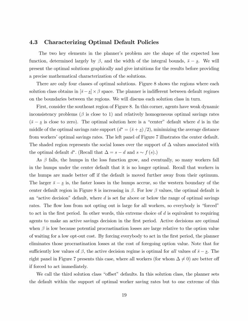
There are only four classes of optimal solutions. Figure 8 shows the regions where each

solution class obtains in [�s� s]�� space. The planner is indi¤erent between default regimeson the boundaries between the regions. We will discuss each solution class in turn.

First, consider the southeast region of Figure 8. In this corner, agents have weak dynamic

inconsistency problems (� is close to 1) and relatively homogeneous optimal savings rates

(�s � s is close to zero). The optimal solution here is a �center�default where d is in themiddle of the optimal savings rate support (d� = (�s+ s) =2), minimizing the average distance

from workers�optimal savings rates. The left panel of Figure 7 illustrates the center default.

The shaded region represents the social losses over the support of � values associated with

the optimal default d�: (Recall that � = s� d and s � f (s).)As � falls, the humps in the loss function grow, and eventually, so many workers fall

in the humps under the center default that it is no longer optimal. Recall that workers in

the humps are made better o¤ if the default is moved further away from their optimum.

The larger �s � s is, the faster losses in the humps accrue, so the western boundary of thecenter default region in Figure 8 is increasing in �. For low � values, the optimal default is

an �active decision�default, where d is set far above or below the range of optimal savings

rates. The �ow loss from not opting out is large for all workers, so everybody is �forced�

to act in the �rst period. In other words, this extreme choice of d is equivalent to requiring

agents to make an active savings decision in the �rst period. Active decisions are optimal

when � is low because potential procrastination losses are large relative to the option value

of waiting for a low opt-out cost. By forcing everybody to act in the �rst period, the planner

eliminates those procrastination losses at the cost of foregoing option value. Note that for

su¢ ciently low values of �, the active decision regime is optimal for all values of �s� s. Theright panel in Figure 7 presents this case, where all workers (for whom � 6= 0) are better o¤if forced to act immediately.

We call the third solution class �o¤set�defaults. In this solution class, the planner sets

the default within the support of optimal worker saving rates but to one extreme of this

19

range so that workers fall into only one of the two humps. O¤set defaults are optimal when

both �s� s and � are large (the northeast region of Figure 8). The center panel of Figure 7illustrates such a scenario. The o¤set default is a compromise between the active decision

and center solutions. Because agents show little dynamic inconsistency, it is not e¢ cient to

force everyone to opt out in the �rst period when many could gain from being allowed to

wait for a low-cost period to act. On the other hand, the range of optimal savings rates is

large enough that a center solution would place too many workers in the humps. By using

an o¤set default, the planner bene�cially moves population mass from one of the humps to

a plateau, while still letting those with optimal rates near the new default exploit the option

value of waiting.

We can also characterize the boundaries of the o¤set default region. Figure 8 shows

that the indi¤erence curve between the o¤set and active decision regions is vertical. This is

because if the heterogeneity of agents�optimal savings rates increased slightly, the marginal

saver at the boundary of the � support would be compelled to act immediately under both

regimes. Thus, changing �s� s cannot make one regime more attractive than the other; only� can change this relation.

Now consider the boundary of this region when � = 1. In this case, the agent is time-

consistent, so the expected loss function is weakly increasing in j�j, as in the left panel ofFigure 7. The center default is always a solution for this scenario. But if �s�s is large enoughthat some workers always opt out immediately under the center default, the planner can move

the default slightly away from the center without a¤ecting the average loss function, since

workers at both boundaries of ��s support are still acting immediately. Thus, the solution

set when � = 1 and �s� s is large includes a neighborhood around the center default.Another interesting property of these optimal policies is the existence of a �global indif-

ference point�at which the center default, o¤set default, and active decision regimes produce

equal total expected losses for workers. We can also prove that the active decision region

grows when the loss from a given deviation from one�s optimal savings rate� controlled by the

parameter �� increases. Increasing the volatility of opt-out costs (i.e., raising �c�c) increasesthe option value to waiting for a low-cost period and hence decreases the attractiveness of

extreme defaults that compel immediate action.

In the following subsection, we formalize the heuristic analysis presented above. Readers

not interested in the mathematical details of the optimal defaults should skip this subsection.

20

4.3.1 Optimal Defaults: A Formal Characterization

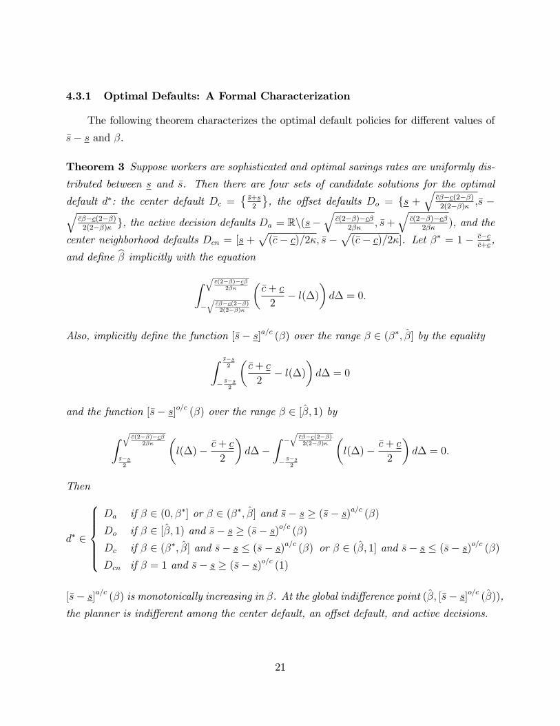
The following theorem characterizes the optimal default policies for di¤erent values of

�s� s and �.

Theorem 3 Suppose workers are sophisticated and optimal savings rates are uniformly dis-

tributed between s and �s. Then there are four sets of candidate solutions for the optimal

default d�: the center default Dc =��s+s2

, the o¤set defaults Do = fs +

q�c��c(2��)2(2��)� ;�s �q

�c��c(2��)2(2��)� g, the active decision defaults Da = Rn(s�

q�c(2��)�c�

2��; �s+

q�c(2��)�c�

2��), and the

center neighborhood defaults Dcn = [s +p(�c� c)=2�; �s �

p(�c� c)=2�]. Let �� = 1 � �c�c

�c+c,

and de�ne b� implicitly with the equationZ q

�c(2��)�c�2��

�q

�c��c(2��)2(2��)�

��c+ c

2� l(�)

�d� = 0:

Also, implicitly de�ne the function [�s� s]a=c (�) over the range � 2 (��; �] by the equality

Z �s�s2

� �s�s2

��c+ c

2� l(�)

�d� = 0

and the function [�s� s]o=c (�) over the range � 2 [�; 1) by

Z q�c(2��)�c�

2��

�s�s2

�l(�)� �c+ c

2

�d��

Z �q

�c��c(2��)2(2��)�

� �s�s2

�l(�)� �c+ c

2

�d� = 0:

Then

d� 2

8>>>><>>>>:Da if � 2 (0; ��] or � 2 (��; �] and �s� s � (�s� s)a=c (�)Do if � 2 [�; 1) and �s� s � (�s� s)o=c (�)Dc if � 2 (��; �] and �s� s � (�s� s)a=c (�) or � 2 (�; 1] and �s� s � (�s� s)o=c (�)Dcn if � = 1 and �s� s � (�s� s)o=c (1)

[�s� s]a=c (�) is monotonically increasing in �. At the global indi¤erence point (�; [�s� s]o=c (�)),the planner is indi¤erent among the center default, an o¤set default, and active decisions.

21

The theoretical appendix contains the proof of this theorem, but we provide a heuristic

proof here.

The proof begins by establishing basic properties for l(�), including symmetry, continuity,

and di¤erentiability at all points except the knots. Next, we identify those regions of l(�)

which lie above �c+c2. We also calculate the derivatives of l and prove that l(�) has global

maxima at � = �q

(�c�c)2�c2(1��)22(�c�c)�(2��)� and a global minimum at � = 0. The next step shows

that if a and b are on di¤erent sides of the same hump and l(a) = l(b), then jl0(a)j < jl0(b)j;in other words, the outer portion of the humps is steeper than the portion closer to � = 0.

This fact is critical because it implies that, starting from the maximum of l at the top of

each hump, the expected loss for workers falls faster when they move away from the default

than when they move towards it. After showing that @l@�� 0, we complete the preliminary

analysis by solving for the �rst and second order conditions of the planner�s maximization

problem and identifying the three candidate solution sets.

We then characterize the optimal solutions. When � 2 (0; ��], we prove that active de-cisions are the only possible solution. Because l(�) > �c+c

2for all � 6= 0, the proof is trivial.

Similarly, when � = 1, the center default� as well as those defaults in the immediate neigh-

borhood for large enough �s� s�must always be optimal because of the weak monotonicityof l(�) in j�j.The �nal step of the proof is to choose among the multiple candidate solutions in the large

intermediate range where � 2 (��; 1) by determining the boundaries between the regions. Inaddition, we formalize the intuition given above for the positive monotonicity of the boundary

between the active decision and center default regions. We also prove the existence of the

global indi¤erence point by transitivity of the planner�s preferences.

4.4 The Case of Naive Workers

Our analysis to this point has assumed that workers understand their own time incon-

sistency. Our qualitative conclusions do not change if we assume instead that workers are

naive about their self-control problems and believe they will be time-consistent in the future

(O�Donoghue and Rabin 1999a,b). While the mathematics behind the optimal default pol-

icy for naive workers is di¤erent from that for sophisticated agents, the intuition is similar.

Workers who exhibit quasi-hyberbolic discounting may bene�t from being forced to act in

22

the �rst period regardless of the stochastic opt-out cost.

Theorem 4 For given parameter values, if active decisions are optimal for sophisticated

workers, then active decisions are also optimal for naive workers.

This theorem follows directly from naifs�mistaken belief that their future selves will not

su¤er from dynamic inconsistency. Because of this belief, naifs�expectation of future losses

from inaction today is lower than sophisticates�correct expectation. Therefore, the naif is

less willing than the sophisticate to incur the stochastic opt-out cost today. Now suppose

the parameter values are such that an active decision regime is optimal for sophisticates.

This implies that sophisticates�self-control problem is bad enough that compelling them to

immediate action is welfare-improving. Naifs, however, have a worse self-control problem

than sophisticates, so an active decision regime must be optimal for naifs as well.

5 Model Discussion

Having characterized the optimal 401(k) enrollment regime, we now connect our theo-

retical results to real-world 401(k) institutions. We classify 401(k) enrollment regimes into

three types: standard enrollment, automatic enrollment, and active decisions.21 Under stan-

dard enrollment, employees have a default savings rate of zero and are given the option

to raise this savings rate. Under automatic enrollment, employees have a default savings

rate that is strictly positive and are given the option to change that savings rate (including

opting out of the plan). Under active decisions, employees face no default and instead must

a¢ rmatively pick their own savings rate.

In our theoretical framework, the standard enrollment regime is an example of an o¤set

default, since a 0% savings rate lies at one end of the optimal savings rate distribution.22 The

automatic enrollment regime, as typically implemented, is an example of an o¤set default

with a low contribution rate, although in some �rms with higher default contribution rates

21The highly successful SMT Plan (Bernartzi and Thaler 2001) is another important type of 401(k) en-rollment regime, but its complexity makes it hard to apply to our model. The SMT Plan has many keyfeatures, including an automatic accelerator that increases the contribution rate at each pay raise.22The standard enrollment default savings rate is on the boundary of the action space, but this location

is consistent with the concept of an o¤set default if savings preferences cross the boundary because somehouseholds would like to dissave.

23

it is more like a center default.23 Finally, a real-world active decision enrollment regime is

equivalent to picking a default contribution rate that is so costly to all workers that everyone

chooses to take action immediately and move to his or her individually optimal savings rate.

When � is close to one, a center default is optimal if employee savings preferences are

relatively homogeneous. In practice, employees will have relatively homogeneous savings

preferences when the workforce is demographically homogeneous (e.g., has a narrow range

of ages) or if a generous employer match causes most employees to want to save at the

match threshold. As savings preferences become more heterogeneous, o¤set defaults such

as standard enrollment and automatic enrollment with conservative defaults become more

attractive. Standard enrollment and automatic enrollment with conservative defaults are

also more attractive when a substantial fraction of employees have a low optimal savings

rate in the 401(k). This may be the case if the company o¤ers a generous de�ned bene�t

pension, if the company employs many low-wage workers who will have a high Social Security

replacement rate, or if the company employs primarily young workers who would like to

dissave at the present because they expect high future income growth.

If employees have a strong tendency to procrastinate (� is far below one), then active

decisions are optimal regardless of how heterogeneous savings preferences are.24 The long-

run stickiness of the default savings rate and asset allocation under automatic enrollment

(Madrian and Shea 2001; Choi et al 2004) supports the concern that many employees have

an excessive tendency to delay opting out of defaults; it typically takes more than two years

for the median employee to opt out of a 2 or 3% savings rate default. Active decisions

eliminate the procrastination problem at the expense of losing the option value of waiting

for a low-cost period to act.

6 Conclusion

This paper identi�es and analyzes the active decision alternative to default-based 401(k)

enrollment processes. The active decision approach forces employees to explicitly choose

23Choi et al (2004) report that three-quarters of companies with automatic enrollment set their defaultcontribution rate at 2% or 3% of pay, which is much lower than the 7% average 401(k) savings rate selectedby employees when they make an a¢ rmative choice.24However, in the limit case of zero heterogeneity, the planner should adopt automatic enrollment with a

default at the universal optimal savings rate.

24

between the options of enrollment and non-enrollment in the 401(k) plan without advantaging

either of these outcomes. We �nd that the fraction of employees who enroll in the 401(k)

three months after hire is 28 percentage points higher under an active decision regime than

under a standard opt-in enrollment regime. The active decision regime also raises average

saving rates and accumulated 401(k) balances. The distribution of new employees�savings

rates under active decisions matches the distribution it takes three years to achieve under

standard enrollment.

We also present a model of the employee�s 401(k) enrollment choice. Under this frame-

work, three socially optimal 401(k) enrollment procedures emerge. We describe conditions

under which the optimal enrollment regime is either automatic enrollment (i.e., default en-

rollment), standard opt-in enrollment (i.e., default non-enrollment), or active decisions (i.e.,

no default and compulsory choice). The active decision regime is socially optimal when

consumers have heterogeneous savings preferences and a strong tendency to procrastinate.

Although active decision 401(k) enrollment regimes are not widely utilized today, we

anticipate that the evidence reported in this paper will lead to broader adoption of such

schemes. In the current technological environment, an active decision enrollment regime

need not necessarily take the form of the paper-and-pencil system that we studied. Instead,

active decision systems could be designed to take advantage of the e¢ ciencies available with

electronic enrollment. For example, a �rm could require new employees to visit a Web site

where they would actively elect to enroll in or opt out of the 401(k) plan, perhaps in conjunc-

tion with electing other bene�ts or providing other information relevant to the company.25

Firms could also compel non-participating employees to make an active decision during each

annual open enrollment period. This would ensure that non-participating employees rethink

their non-participation in the 401(k) at least once a year.

The active decision approach to increasing 401(k) participation has some attractive fea-

tures relative to other savings promotion schemes. Compared to �nancial education, re-

quiring an active decision is a more cost-e¤ective way to boost 401(k) participation. Active

decisions are also more cost-e¤ective than increasing the employer match rate, since increases

in the match rate apply even to employees who would have enrolled with little or no match.

Finally, requiring individuals to make an active decision represents a weaker alternative to

the standard paternalism implicit in specifying a default that will advantage one particular

25Workers without access to computers could submit paper forms.

25

course of action over another. Active decision interventions are designed principally to force

a decision-maker to think about a problem. This is still a type of paternalism, but it does

not presuppose an answer to the problem.26

We should note that we are not opposed to �nancial education, employer matching, or

automatic enrollment. Rather, we view all of these, along with active decisions, as potentially

complementary approaches to fostering increased and higher-quality 401(k) participation.

These tools, when implemented well, can greatly enhance the retirement income security of

a company�s current and future employees.

Active decision interventions will be useful in many situations where consumer het-

erogeneity implies that one choice isn�t ideal for everyone (e.g., the selection of a health

plan or automobile insurance27) and �rms or governments feel uncomfortable implementing

employee-speci�c defaults (e.g., if such employee-speci�c defaults are viewed as �advice�

with �duciary consequences).28 In contrast, defaults will have a natural role to play in cases

where a large degree of homogeneity is appropriate and household decision-makers have lim-

ited expertise (e.g., portfolio allocation).29 Future research should explore active decision

experiments in other decision domains and compare the relative e¢ cacy of active decision

and default-based systems, as well as hybrid systems which may turn out to be the most

useful approach of all.

26We view active decisions as an example of libertarian paternalism (Sunstein and Thaler 2003).27The active decision approach to purchasing automobile insurance is widely used. Drivers cannot, in

general, register their cars without obtaining insurance. But the government does not specify a defaultinsurance contract for drivers; rather, it requires drivers to obtain their own insurance� to make an activedecision. The model in the paper suggests that there is a good justi�cation for this approach: there is likelyto be substantial heterogeneity in individual preferences over insurance policy types and companies.28An example of an intriguing employee-speci�c default is a default savings rate that increases with the

employee�s age.29See Benartzi and Thaler (2003) and Cronqvist and Thaler (2004) for evidence on poor asset allocation

choices.

26

7 Appendix

7.1 The Sophisticated Worker�s Optimization Problem

Proposition 1 A sophisticated worker will opt out of the default if and only if she draws a

transaction cost c < c�, where

c� =c+

pc2 [1� (2� �)�] + 2� (2� �) (�c� c)L

2� � : (7)

Proof. Fix d. Note that if s 6= d, then c� > c; otherwise the agent would never act and

would lose W = L+ �P1

t=1 L =1. Also, the agent must be indi¤erent between acting andnot acting in the present, so

c� = � [L+ EV (L; c0; c�)] (8)

where

V (L; c0; c�) =

(c0 if c0 < c�

L+ E+1V (L; c00; c�) if c0 � c�

; (9)

c0is the cost draw for the current period, and c

00is the cost draw for the following period.

Letting � = EV (L; c0; c�), at c� the function V (�) must also be a �xed point for the futurevalue function. Generalizing over periods and then integrating over draws of c implies that

� =c�2 � 2Lc� + 2L�c� c2

2 (c� � c) : (10)

Substituting (10) into (8) gives us a quadratic equation in c�. Using the quadratic formula

and choosing the upper root so that c� > c, we obtain equation (7).

Proposition 2 The worker�s expected loss function from the planner�s perspective is

l(�) =

8>>><>>>:0 if � = 0p2(�c�c)�(2��)��2+(1��)2c2

�(2��) � ��2 + c�(2��) if 0 < j�j <

q�c(2��)�c�

2��

�c+c2

ifq

�c(2��)�c�2��

< j�j

: (11)

Proof. The expected loss function for workers from the planner�s perspective is exactly

27

EV (L; c0; c�) if c < c� < �c. Substituting (7) into (10) yields

l(�) =

q2(�c� c)� (2� �)��2 + (1� �)2 c2

�(2� �) � ��2 +c

�(2� �) :

If c� � �c, the agent will act immediately regardless of the opt-out cost. In this case, l(�) =�c+c2, the average opt-out cost drawn in the �rst period. The condition c� � �c holds when

j�j <

s�c(2� �)� c�

2��:

Finally, the agent never opts out or incurs any �ow losses when � = 0, so l (�) = 0.

7.2 The Planner�s Optimization Problem

Before proving Theorem 3, we establish several useful lemmas. For notational ease, we

denote the knot point of the function l by K �q

�c(2��)�c�2��

.

Lemma 5 The function l(�) is symmetric around � = 0, continuous when � 6= 0, and

twice-di¤erentiable with respect to all its parameters when � 6= 0 and � 6= �K.

Going forward, we assume � � 0; the case � < 0 is equivalent by the symmetry of the

function l (�) : We now prove some lemmas regarding the shape of l. It is useful to de�ne

�� = 1 � �c�c�c+c. We �rst characterize l for � 2 (0; ��] and then move on to the case where

� 2 (��; 1].

Lemma 6 If � 2 (0; ��], then l(�) > �c+c2when 0 < � < K.

Proof. The only roots of l(�) = �c+c2over the domain � 2 [0; K] satisfy the condition

��2 =�c� � c(2� �)2 (2� �) or

�c(2� �)� c�2�

(12)

Note that the one of the roots is K and the other does not exist in the proper region of �

when � 2 (0; ��]. Because

l0 (�)j�!K�= �2�K

�(1� �)�c

(2� �) �c� c

�< 0;

28

the lemma follows immediately.

At this point, we de�ne E �q

�c��c(2��)2(2��)� and M �

q(�c�c)2�c2(1��)22(�c�c)�(2��)� for notational con-

venience when � 2 (��; 1]. Note that if � 2 (��; 1), then 0 < E < M < K. When � = 1,

E =M = K.

Lemma 7 If � 2 (��; 1), then

� l0(�) > 0 when 0 < � < M

� l0(M) = 0

� l0(�) < 0 when M < � < K

� l0(�) = 0 when K < �

The point � =M is a global maximum. When � = 1;

� l0(�) > 0 when 0 < � < K

� l0(�) = 0 when K � �

Proof. The signing of the derivatives is straightforward. Note that M only exists as a

critical point if

(�c� c)2 � c2 (1� �)2 � 0:

But � 2 (��; 1] implies that

(�c� c)2 � c2 (1� �)2 > (�c� c)2 � c2 (1� ��)2 = 1� c2

(�c+ c)2> 0;

so the critical point always exists in this range of parameters. It is apparent from the signs of

l0(�) over � 2 (0;1) that M is a global maximum. When � = 1, we get M = K =q

�c�c2�.

The part of the function with a downward slope is �squeezed out.�

Lemma 8 If � 2 (��; 1]; then

� l(�) < �c+c2when 0 � � < E

29

� l(E) = �c+c2

� l(�) > �c+c2when E < � < K

Proof. We know from (12) that l(�) = �c+c2when � = K or � = E. Since � > ��, the latter

root exists. Lemma 7 and the continuity of l implies that l(�) > �c+c2when E < � < K and

l(�) < �c+c2when 0 < � < E. That l(0) < �c+c

2is obvious.

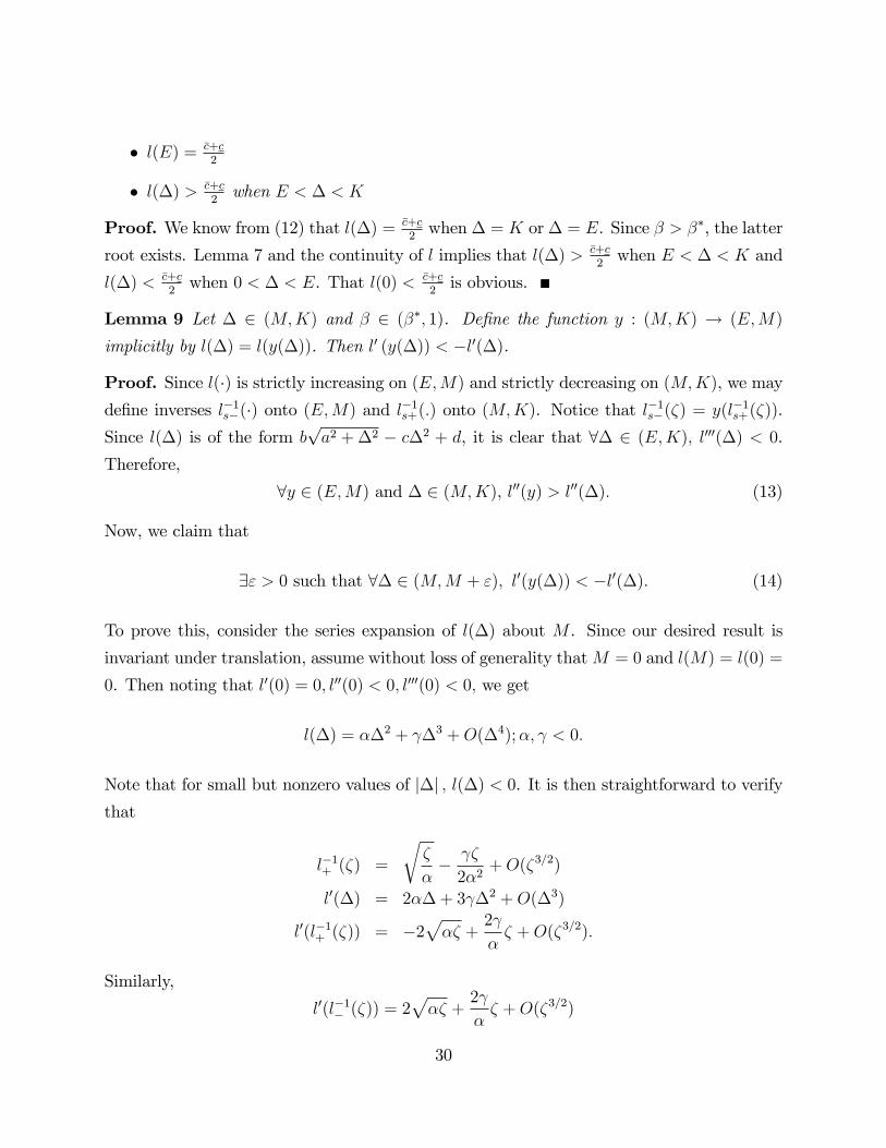
Lemma 9 Let � 2 (M;K) and � 2 (��; 1). De�ne the function y : (M;K) ! (E;M)

implicitly by l(�) = l(y(�)). Then l0 (y(�)) < �l0(�).

Proof. Since l(�) is strictly increasing on (E;M) and strictly decreasing on (M;K), we mayde�ne inverses l�1s�(�) onto (E;M) and l�1s+(:) onto (M;K). Notice that l�1s�(�) = y(l�1s+(�)).

Since l(�) is of the form bpa2 +�2 � c�2 + d, it is clear that 8� 2 (E;K); l000(�) < 0.

Therefore,

8y 2 (E;M) and � 2 (M;K), l00(y) > l00(�): (13)

Now, we claim that

9" > 0 such that 8� 2 (M;M + "); l0(y(�)) < �l0(�): (14)

To prove this, consider the series expansion of l(�) about M . Since our desired result is

invariant under translation, assume without loss of generality thatM = 0 and l(M) = l(0) =

0. Then noting that l0(0) = 0; l00(0) < 0; l000(0) < 0; we get

l(�) = ��2 + �3 +O(�4);�; < 0:

Note that for small but nonzero values of j�j ; l(�) < 0. It is then straightforward to verifythat

l�1+ (�) =

r�

�� �

2�2+O(�3=2)

l0(�) = 2��+ 3 �2 +O(�3)

l0(l�1+ (�)) = �2p�� +

2

�� +O(�3=2):

Similarly,

l0(l�1� (�)) = 2p�� +

2

�� +O(�3=2)

30

Setting � = l�1+ (�), for small but nonzero values of � (which implies small negative values

of �),

l0(y(�)) = l0(l�1� (�)) < �l0(l�1+ (�)) = �l0(�);

which proves (14). Now assume a contradiction to the lemma: 9� 2 (M;K) such that

l0(y(�)) � �l0(�): Let X� � f� : � 2 (M;K); l0(y(�)) � �l0(�)g and �� � inf(X�).

From (14), �� > M . It follows from continuity that l0(y(��)) = �l0(��). Combining this

with (13) and noting that l00(�)

l0 (�)= dl0(�)

d�d�dl(�)

= dl0(�)dl(�)

,

l00(y(��))

l0(y(��))=dl

0(y(��))

dl(y(��))> �dl

0(��)

dl(��)= � l

00(��)

l0(��): (15)

Consider a perturbation of � that increases the value of l (�). From (15) and l0(��) < 0,

we see that 9" > 0 such that l0(y(���")) > �l0(���"). But this contradicts the de�nitionof ��.

The �nal preliminary step characterizes the relationship between l and �.

Lemma 10 @l@�

����< 0 when � 2 (0; K). @l

@�

����= 0 when � =2 (0; K).

Proof. When � = 0, l = 0 always, so @l@�

����=0

= 0. For 0 < � < K, algebra yields

@l

@�= � 2c (1� �)

�2 (2� �)2�(1� �)

�2 (�c� c) � (2� �)��2 + c2

�2 (1� �)2 + � (2� �)

���2 (2� �)2

q2 (�c� c) � (2� �)��2 + c2 (1� �)2

;

which is negative since both fractions are positive. For � � K, @l@�=

@( �c+c2 )@�

= 0:

We now solve the planner�s problem and characterize the optimal solution d�. The result

is presented in a number of lemmas which together imply Theorem 3.

Lemma 11 A solution d� to the planner�s problem must satisfy the conditions

l (�s� d�) = l (s� d�) and l0 (�s� d�) � l0 (s� d�) : (16)

Proof. De�ne Z (d) �R �s�ds�d l(�)d�. The planner will solve the program d

� = argmind Z (d).

The two conditions are the �rst order condition ensuring a stationary point and the second

order condition ensuring a local minimum.

31

Lemma 12 If � 2 (0; ��]; then d� 2 Da, where Da = (�1; s�K][[�s+K;1).

Proof. By Lemma 6, l(�) > �c+c2for all 0 < j�j < K. Thus, if d =2 Da; then

R �s�ds�d l(�)d� >

(�s � s) �c+c2. But if d 2 Da, then

R �s�ds�d l(�)d� = (�s � s) �c+c

2. All d 2 Da trivially satisfy the

�rst and second order conditions in (16).

Lemma 13 If � 2 (��; 1), then all the defaults satisfying the conditions of Lemma 11 aremembers of the set Dc [ Do [ Da, where Dc = f(�s+ s) =2g, Do = fs+ E; �s� Eg, andDa = Rn(s�K; �s+K):

Proof. Points in Dc [Da satisfy the �rst order condition in (16). Points in Do satisfy the

�rst order condition if �s � s � K + E. Lemma 9 implies points in these three sets are the

only ones that can satisfy the second order condition.

Lemma 14 Suppose that � = 1. If �s � s � 2K then d� = �s+s2. If �s � s > 2K then

d� 2 [s+K; �s�K].

Proof. It is easy to verify that the conditions of Lemma 11 are satis�ed for the proposed d�

in both cases. Lemma 7 states that l (�) is weakly increasing in j�j, so the center default�s+s2is always an optimum. If �s � s > 2K, the endpoints of the integral Z( �s+s

2) are outside

[�K;K]. Because l0 (�) = 0 8� =2 (�K;K), the planner is indi¤erent among defaults in theinterval [s+K; �s�K].

Lemma 15 Let �s � s � K + E; so that points in Do satisfy the conditions of Lemma 11.

Then there exists b� 2 (��; 1) such that if � > b�, the planner always prefers a default in Do

to any default in Da. If � < �, the planner always prefers a default in Da to any default in

Do. b� is implicitly de�ned by the equalityZ K(�)

�E(�)l(�)d� =

�c+ c

2(K + E): (17)

Proof. The di¤erence between total expected losses for workers when d� = da 2 Da and

d� = do 2 Do is

Z(da)� Z(do) =Z K

�E

��c+ c

2� l(�)

�d�:

32

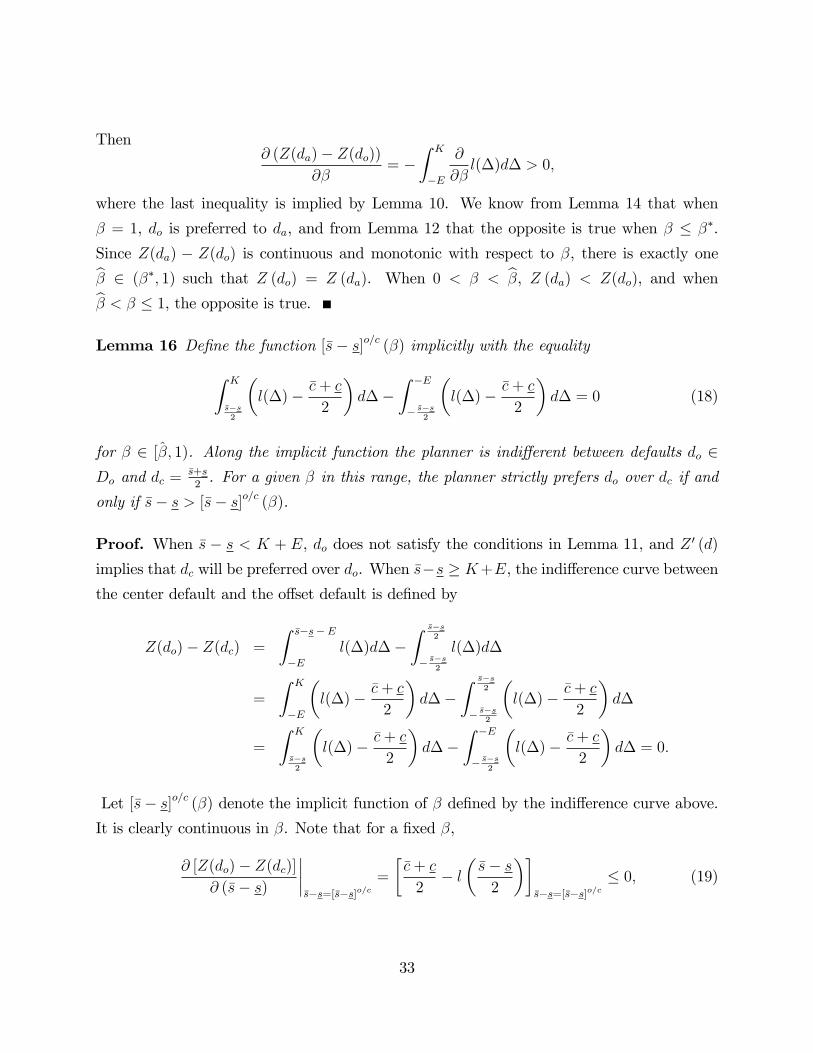
Then@ (Z(da)� Z(do))

@�= �

Z K

�E

@

@�l(�)d� > 0;

where the last inequality is implied by Lemma 10. We know from Lemma 14 that when

� = 1, do is preferred to da, and from Lemma 12 that the opposite is true when � � ��.

Since Z(da) � Z(do) is continuous and monotonic with respect to �, there is exactly oneb� 2 (��; 1) such that Z (do) = Z (da). When 0 < � < b�, Z (da) < Z(do), and whenb� < � � 1, the opposite is true.Lemma 16 De�ne the function [�s� s]o=c (�) implicitly with the equalityZ K

�s�s2

�l(�)� �c+ c

2

�d��

Z �E

� �s�s2

�l(�)� �c+ c

2

�d� = 0 (18)

for � 2 [�; 1). Along the implicit function the planner is indi¤erent between defaults do 2Do and dc =

�s+s2. For a given � in this range, the planner strictly prefers do over dc if and

only if �s� s > [�s� s]o=c (�).

Proof. When �s � s < K + E, do does not satisfy the conditions in Lemma 11, and Z 0 (d)

implies that dc will be preferred over do. When �s�s � K+E, the indi¤erence curve betweenthe center default and the o¤set default is de�ned by

Z(do)� Z(dc) =

Z �s�s� E

�El(�)d��

Z �s�s2

� �s�s2

l(�)d�

=

Z K

�E

�l(�)� �c+ c

2

�d��

Z �s�s2

� �s�s2

�l(�)� �c+ c

2

�d�

=

Z K

�s�s2

�l(�)� �c+ c

2

�d��

Z �E

� �s�s2

�l(�)� �c+ c

2

�d� = 0:

Let [�s� s]o=c (�) denote the implicit function of � de�ned by the indi¤erence curve above.It is clearly continuous in �. Note that for a �xed �,

@ [Z(do)� Z(dc)]@ (�s� s)

�����s�s=[�s�s]o=c

=

��c+ c

2� l��s� s2

���s�s=[�s�s]o=c

� 0; (19)

33

with strict inequality when �s�s2< K. Also, when � 2 (��; 1);

Z(do)� Z(dc)j�s�s �2K = �Z �E

�K

�l(�)� �c+ c

2

�d� < 0 (20)

Z(do)� Z(dc)j�s�s = K + E =

Z K

K+E2

�Z �E

�K+E2

!l(�)d� > 0;

with the latter inequality following from Lemma 9. (19) and (20) imply that [�s� s]o=c (�)exists and is well-de�ned. So when �s� s is above the indi¤erence curve, the o¤set default ispreferred, and the opposite holds for the region below the curve.

Lemma 17 De�ne the function [�s� s]a=c (�) implicitly with the equality

Z �s�s2

� �s�s2

��c+ c

2� l(�)

�d� = 0: (21)

for � 2 [��; �]. Along the implicit function the planner will be indi¤erent between defaultsda 2 Da and dc =

�s+s2. For a given � in this range, the planner strictly prefers da over

dc if and only if �s � s > [�s� s]a=c (�). [�s� s]a=c (��) = 0, and [�s� s]a=c is monotonicallyincreasing with respect to �.

Proof. The indi¤erence curve between the center default and active decisions is de�ned by

Z(da)� Z(dc) = (�s� s)�c+ c

2�Z �s�s

2

� �s�s2

l(�)d� =

Z �s�s2

� �s�s2

��c+ c

2� l(�)

�d� = 0:

Let [�s� s]a=c denote the implicit function of � de�ned by the indi¤erence curve above. Now

@ [Z(da)� Z(dc)]@ (�s� s)

�����s�s=[�s�s]a=c

=

��c+ c

2� l��s� s2

���s�s =[�s�s]a=c

< 0; (22)

since l( �s�s2) must be greater than �c+c

2due to the planner�s indi¤erence between the center

default and active decisions. Also, (20) holds for � 2 (��; �), which gives us

Z(da)� Z(dc)j�s�s �2K < Z(do)� Z(dc) = �Z �E

�K

�l(�)� �c+ c

2

�d� < 0; (23)

34

where the �rst inequality comes from Lemma 15. In addition,

Z(da)� Z(dc)j�s�s� E � (�s� s)��c+ c

2� l(0)

�> 0: (24)

(22), (23), and (24) establish existence and uniqueness of [�s� s]a=c (�). For a �xed �, dc isoptimal when �s�s is below [�s� s]a=c (�) and da is optimal when �s�s is above [�s� s]a=c (�).When � = ��, lim�!0 l(�) =

�c+c2, so by Lemma 6, Z(da) < Z(dc) if �s � s > 0. Therefore,

we may de�ne [�s� s]a=c (��) = 0. Using the Implicit Function Theorem, (22), and Lemma10, we have

d [�s� s]a=c

d�= � @ (Z(da)� Z(dc)) =@�

@ (Z(da)� Z(dc)) =@(�s� s)> 0:

Thus the indi¤erence boundary is well-de�ned, and monotonically increasing in �.

Lemma 18 If � 2 (��; 1), then [�s� s]a=c (�) = [�s� s]o=c (�) if and only if � = �. That is,the three indi¤erence boundaries intersect at a unique global indi¤erence point in the (�; �s�s)space.

Proof. We know from the proof of Lemma 16 that the planner is indi¤erent between the

center default and the o¤set default along [�s� s]o=c and that [�s� s]o=c (�) � K+E. We knowfrom Lemma 15 that when �s� s � K +E and � = �, the planner is indi¤erent between theo¤set default and active decisions. Therefore, by transitivity, the planner must be indi¤erent

between the center default and active decisions at (�; [�s� s]o=c (�)). This global indi¤erencepoint must be unique because the planner is indi¤erent between active decisions and the

o¤set default only when � = �, and the indi¤erence curves take only one value each at �.

Theorem 3 See the body of the paper for the full statement of this theorem.

Proof. This theorem, as it appears in the body of the paper, combines the Lemmas in this

Appendix into one statement. Lemma 13 establishes the three classes of optimal defaults

when � < 1. The indi¤erence curves for the region � 2 (��; 1) are de�ned in Lemmas 15, 16,and 17. The regions where each default class is optimal are also described in these Lemmas.

The optimal default policies for the region � 2 (0; ��) and � = 1 are derived in Lemmas

12 and 14. Lemma 17 proves the monotonicity of [�s� s]a=c (�). Lemma 18 establishes theexistence of a unique global indi¤erence point.

35

The following theorem states a comparative static on optimal defaults as � increases.

Theorem 19 The optimal default class for a set of parameter values including loss constant

� and optimal savings range �s�s is also the optimal default class for a setting where the lossconstant is ��; the optimal savings rate range is (�s � s)=

p�; and all other parameters are

unchanged. The set of pairs f�; �s� sg where active decisions are optimal strictly increasesas one increases �. Formally, @�

1=2[�s�s]a=c@�

= 0 and @��

@�= @�

@�= 0.

Proof. Since � only appears in l as ��2, if we de�ne �0 � �� and �0 � �=p�, then

l (�)j� = l (�0)j�0 8�, provided � > 0. It follows that 8d,Z �s�d

s�dl (�)j� d� =

Z (�s�d)=p�

(s�d)=p�

l(�0)j�0p�d�0 (25)

This implies that if d is optimal when the loss constant is �, the maximum optimal

savings rate is �s, and the minimum optimal savings rate is s, then d=p� will be optimal

when the loss constant is ��, the maximum optimal savings rate is �s=p�, and the minimum

optimal savings rate is s=p�. It is easy to verify that d and d=

p� belong to the same default

class within their respective parameter settings. It is also trivial to show that holding all

other parameters �xed, the optimal default class depends only on the distance between the

maximum and minimum optimal savings rates, not their values individually. Applying (25)

to the de�nition of [�s� s]a=c in (21) yields the result that [�s� s]a=c is inversely proportionaltop�, so @�1=2[�s�s]a=c

@�= 0. It is obvious from the de�nition of �� that @�

�

@�= 0. To establish

that @�@�= 0, we show that if a given value of � satis�es (17) under parameter value �, then

it also satis�es the relation under parameter value �0. Note that the values of E and K are

functions of �, E (�) =p�E (�0), and K (�) =

p�K (�0). Then for a given value of �,

Z K(�0)

�E(�0)l(�0)j�0 d�0 =

1p�

Z K(�)

�E(�)l(�)j� d�

=�c+ c

2

�K(�) + E(�)p

�

�=

�c+ c

2(K(�0) + E(�0)) ;

where the second equality results from (17) being true under parameter values � and �.

36

7.3 The Case of Naive Workers

Lemma 20 @c�

@�> 0.

Proof.

@c�

@�=c�p

c2 (1� (2� �)�) + 2� (1� �) (�c� c)L� c (1� �)�+ 2 (2� �) (�c� c)L

(2� �)2pc2 (1� (2� �)�) + 2� (1� �) (�c� c)L

(26)

is positive, since both parts of the numerator are positive.

Theorem 4 For given parameter values, if active decisions are optimal for sophisticated

workers, then active decisions are also optimal for naive workers.

Proof. Consider the naive workers� future optimization problem from their current per-

spective. Naive workers believe they will act as if they were time-consistent exponential

discounters (� = 1) in the future. Therefore, they anticipate using a cuto¤ cost c�e in the

future when deciding whether to opt out, where

c�e = argminc�E (V (L; c0)) = argmin

c�

(c0 if c0 � c�

L+ E (V (L; c00)) if c0 > c�: (27)

Sophisticates understand that they will use the same cuto¤cost c�s both today and tomorrow.

Thus, \E (V (L)jnaive) � \E (V (L)jsoph), where \E (V (L)) represents the worker�s perceivedfuture loss expectation for herself. The inequality is strict if � < 1 by Lemma 20.

The naifs�current cuto¤ cost will be chosen such that

c�n = �(L+\E (V (L)jnaive)):

Since \E (V (L)) is lower for naive workers than for sophisticated workers, c�n � c�s, with theinequality strict if � < 1. Furthermore, we know that c�s < c

�e when � < 1 by Lemma 20.

Note that agents using a cuto¤ rule c� will act with probability p = c��c�c�c and pay an

average transaction cost ~c = c�+c2when they act. Thus,

l(c�; L) = p~c+ (1� p) p (L+ ~c) + (1� p)2 p (2L+ ~c) + � � �

=c� + c

2+�c� c�c� � cL:

37

Note that c�e is the point which minimizes this function. Let le (�), ls (�), and ln (�) be

the expected loss functions for agents using cuto¤ values c�e, c�s, and c

�n, respectively. Then

the convexity of l and the ordering c�n � c�s � c�e implies that le(�) � ls(�) � ln(�) when0 < j�j < K, with strict inequalities when � < 1. We have assumed in the statement

of the theorem that active decisions are optimal for sophisticates (which only holds when

� < 1). Therefore, 8d 2 (s�K; �s+K),R �s�ds�d ln(�)d� >

R �s�ds�d ls(�)d� > (�s� s)

�c+c2, where

the last term is the total loss under active decisions. Hence, when active decisions are best

for sophisticates, they are best for naifs.

8 References

Abadie, Alberto, and Sebastien Gay (2004). �The Impact of Presumed Consent Legislation

on Cadaveric Organ Donation: A Cross Country Study,�NBER Working Paper No.

10604.

Aguiar, Mark, and Erik Hurst (2004). �Consumption vs. Expenditure,� University of

Chicago Working Paper.

Benartzi, Shlomo, and Richard H. Thaler (2001). �Naive Diversi�cation Strategies in De-

�ned Contribution Saving Plans,�American Economic Review 91(1): 79-98.

Choi, James J., David Laibson, Brigitte C. Madrian, and Andrew Metrick (2004). �For

Better or For Worse: Default E¤ects and 401(k) Savings Behavior,�in David A. Wise,

ed., Perspectives in the Economics of Aging (Chicago, IL: University of Chicago Press):

81-121.

Choi, James J., David Laibson, Brigitte C. Madrian, and Andrew Metrick (2002). �De-

�ned Contribution Pensions: Plan Rules, Participant Decisions, and the Path of Least

Resistance,�in James M. Poterba, ed., Tax Policy and the Economy 16, (Cambridge,

MA: MIT Press): 67-113.

Cronqvist, Henrik, and Richard H. Thaler (2004). �Design Choices in Privatized Social-

Security Systems: Learning from the Swedish Experience,�American Economic Review

94(2): 424-428.

38

Engen, Eric M., William G. Gale, and Cori E. Uccello (1999). �The Adequacy of Household

Saving,�Brookings Papers on Economic Activity 0(2): 65-165.

Even, William E., and David MacPherson (1999). �Employee Participation in 401(k)

Plans,�Florida State University Working Paper.

Hurst, Erik (2004). �Grasshoppers, Ants and Pre-Retirement Wealth: A Test of Permanent

Income Consumers,�University of Chicago Working Paper.

John Hancock (2002). �Eighth De�ned Contribution Plan Survey: Insight Into Participant

Knowledge & Behavior.�(Boston, MA: John Hancock Financial Services).

Johnson, Eric J., and Daniel Goldstein (2003). �Do Defaults Save Lives?,�Science 302(No-

vember 21): 1338-1339.

Johnson, Eric J., John Hershey, Jacqueline Meszaros, and Howard Kunreuther (1993).

�Framing, Probability Distortions, and Insurance Decisions,�Journal of Risk and Un-

certainty 7(1): 35-53.

Johnson, Eric J., Steven Bellman, and Gerald L. Lohse (2002). �Defaults, Framing and

Privacy: Why Opting In-Opting Out,�Marketing Letters 13(1): 5-15.

Laibson, David (1997).�Golden Eggs and Hyperbolic Discounting,�Quarterly Journal of

Economics 112(2): 443-477.

Madrian, Brigitte C., and Dennis Shea (2001). �The Power of Suggestion: Intertia in

401(k) Participation and Savings Behavior,�Quarterly Journal of Economics 116(4):

1149-1187.

O�Donoghue, Ted, and Matthew Rabin (1999a). �Procrastination in Preparing for Re-

tirement,� in Henry J. Aaron, ed., Behavioral Dimensions of Retirement Economics

(Washington, D.C.: Brookings Institution Press; New York, NY: Russell Sage Foun-

dation): 125-156.

O�Donoghue, Ted, and Matthew Rabin (1999b). �Doing It Now or Later,�American Eco-

nomic Review 89(1): 103-124.

39

Park, C. Whan, Sung Y. Jun, and Deborah J. MacInnis (2000). �Choosing What I Want

Versus RejectingWhat I Do NotWant: An Application of Decision Framing to Product

Option Choice Decisions,�Journal of Marketing Research 37(2): 187-202.

Phelps, Edmund S., and Robert A. Pollak (1968). �On Second-Best National Savings and

Game-Equilibrium Growth,�Review of Economic Studies 35(2): 185-199.

Sunstein, Cass R., and Richard H. Thaler (2003). �Libertarian Paternalism,�American

Economic Review 93(2): 175-179.

Thaler, Richard H., and Shlomo Benartzi (2004). �Save More TomorrowTM: Using Behav-

ioral Economics to Increase Employee Saving,�Journal of Political Economy 112(1):

S164-187.

Warshawsky, Mark J., and John Ameriks (2000). �How Prepared Are Americans for Re-

tirement?,�in Olivia S. Mitchell, P. Brett Hammond, and Anna M. Rappaport, eds.,

Forecasting Retirement Needs and Retirement Wealth (Philadelphia, PA: University of

Pennsylvania Press): 33-67.

40

Tab

le 1

. 401

(k)

plan

feat

ures

by

effe

ctiv

e da

te

E

ffect

ive

Janu

ary

1, 1

997

Effe

ctiv

e N

ovem

ber

23, 1

997

Elig

ibili

ty

Elig

ible

em

ploy

ees

U.S

. em

ploy

ees, a

ge 1

8+

U.S

. em

ploy

ees,

age

18+

Fir

st e

ligib

le

Imm

edia

tely

upo

n hi

re

Imm

edia

tely

upo

n hi

re

Em

ploy

er m

atch

elig

ible

Im

med

iate

ly u

pon

hire

Im

med

iate

ly u

pon

hire

Enr

ollm

ent

First

30

days

of em

ploy

men

t or

Jan

uary

1 o

f

succ

eedi

ng c

alen

dar

year

s

Dai

ly

Con

trib

utio

ns

Em

ploy

ee c

ontr

ibut

ions

U

p to

17%

of c

ompe

nsat

ion

Up

to 1

7% o

f co

mpe

nsat

ion

Non

-dis

cret

iona

ry e

mpl

oyer

mat

ch

50%

of e

mpl

oyee

con

trib

utio

n up

to

5% o

f

com

pens

atio

n

50%

of em

ploy

ee c

ontr

ibut

ion

up t

o 5%

of

com

pens

atio

n

Dis

cret

iona

ry e

mpl

oyer

mat

ch

Up

to 1

00%

of em

ploy

ee c

ontr

ibut

ion

depe

ndin

g on

com

pany

pro

fitab

ility

(50

% for

bon

us-e

ligib

le

empl

oyee

s); 1

00%

in 1

997.

Up

to 1

00%

of em

ploy

ee c

ontr

ibut

ion

depe

ndin

g on

com

pany

pro

fitab

ility

(50

% fo

r bo

nus-

elig

ible

empl

oyee

s); v

arie

d fr

om 0

% t

o 10

0% fo

r 19

97-2

000.

a

Ves

ting

Im

med

iate

Imm

edia

te

Oth

er

Loan

s N

ot a

vaila

ble

Ava

ilabl

e; 2

max

imum

Har

dshi

p w

ithd

raw

als

Ava

ilabl

e A

vaila

ble

Inve

stm

ent

choi

ces

6 op

tion

s. E

mpl

oyer

sto

ck a

lso

avai

labl

e, b

ut o

nly

for

afte

r-ta

x co

ntribu

tion

s.

8 op

tion

s +

em

ploy

er s

tock

(av

aila

ble

for

befo

re-

and

afte

r-ta

x co

ntri

buti

ons)

a A

ctua

l dis

cret

iona

ry m

atch

rat

es fo

r 19

95-2

001

wer

e 20

% (

1995

), 2

0% (

1996

), 1

00%

(19

97), 1

00%

(19

98), 2

7% (

1999

), 3

3% (

2000

), 0

% (

2001

).

Table 2. Comparison of worker characteristics

Study company

Active decision

cohort

on 12/31/98

Standard

enroll. cohort

on 12/31/99

All

workers

on 12/31/99

U.S.

workforce

(3/98 CPS)

Average age (years) 34.1 34.0 40.5 38.8

Gender

Male 45.4% 43.4% 45.0% 53.1%

Female 54.6% 56.6% 55% 46.9

Marital Status

Single 42.8% 47.8% 32.4% 39.0%

Married 57.2% 52.2% 67.6% 61.0%

Compensation

Avg. monthly base pay $2,994 $2,911 $4,550 --

Median monthly base pay $2,648 $2,552 $3,750 --

Avg. annual incomea $34,656 $34,001 $52,936 $32,414

Median annual incomea $30,530 $29,950 $42,100 $24,108

Geography

East 10.0% 8.4% 12.1% 18.9%

Midwest 37.9% 39.8% 35.3% 24.1%

South 37.1% 39.0% 37.8% 34.7%

West 15.0% 12.6% 14.7% 22.4%

Number of Employees 2,205 2,344 46,822 --

The samples in the first three columns are taken from individuals employed at the study company as of

the dates indicated in the column title. The sample in the last column is all individuals in the March 1998

Current Population Survey who worked in the previous year (weighted). aThe annual income measure that is reported to us for the study company is the employee�s annual taxable

(W2) income. Annual income for the U.S. workforce calculated from the CPS is total annual labor

earnings in the previous calendar year, some of which may be non-taxable.

Table 3. Regression of contribution rates under two 401(k) enrollment regimes

Intercept -8.125**

(1.998)

Married 1.239**

(0.251)

Log(Base pay) 1.985**

(0.223)

0 ≤ Age < 30 -4.003**

(1.061)

30 ≤ Age < 40 -3.311**

(1.060)

40 ≤ Age < 50 -2.688**

(1.076)

50 ≤ Age < 60 -1.755

(1.105)

Active decision cohort 3.258

(3.410)

Active decision cohort × Married -0.963**

(0.396)

Active decision cohort × Log(Base pay) -0.064

(0.385)

Active decision cohort × (0 ≤ Age < 30) -2.381

(1.571)

Active decision cohort × (30 ≤ Age < 40) -2.047

(1.573)

Active decision cohort × (40 ≤ Age < 50) -1.988

(1.598)

Active decision cohort × (50 ≤ Age < 60) -0.517

(1.667)

R2 0.12

N 2,422

If the employee is in the active decision cohort, the dependent variable is the 401(k) contribution rate (in

percentage points) three months after hire; if the employee is in the standard enrollment cohort, the

dependent variable is the contribution rate three years after hire. Dependent variables are calculated as of

the contribution rate date. Married is a dummy that equals one if the employee is married. The variables

n1 ≤ Age < n2 are dummies that equal one if the employee�s age falls within the specified range. Active

decision cohort is a dummy that equals one if the employee is in the active decision cohort. Standard

errors are reported in parentheses under the point estimates.

*Significant the 5% level

**Significant at the 1% level

66%71% 70% 70%

63%67%

73%

45% 42% 43% 40%35%

40% 41%

0%

10%

20%

30%

40%

50%

60%

70%

80%

90%

January February March April May June July

Month of Hire

Frac

tion

enro

lled

in th

e 40

1(k)

pla

n at

third

mon

th o

f ten

ure

Active decision cohort Standard enrollment cohort

Figure 1. Fraction of employees enrolled in the 401(k), by hire month. The fraction displayed is as of the

end of the third month of tenure at the company. The active decision cohort was hired between January

and July 1997. The standard enrollment cohort was hired between January and July 1998.

0%

10%

20%

30%

40%

50%

60%

70%

80%

90%

100%

0 5 10 15 20 25 30 35 40 45 50 55

Tenure at company (months)

Frac

tion

enro

lled

in th

e 40

1(k)

pla

n

Active decision cohort Standard enrollment cohort

Figure 2. Fraction of employees enrolled in the 401(k) plan, by tenure at company. An employee is

counted enrolled in the 401(k) plan even if he or she is not currently contributing to the plan. The series

are not monotonically rising because they are constructed from multiple cross-sections, so the samples are

not fixed over time.

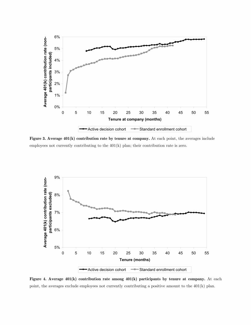
0%

1%

2%

3%

4%

5%

6%

0 5 10 15 20 25 30 35 40 45 50 55

Tenure at company (months)

Ave

rage

401

(k) c

ontr

ibut

ion

rate

(non

-pa

rtic

ipan

ts in

clud

ed)

Active decision cohort Standard enrollment cohort

Figure 3. Average 401(k) contribution rate by tenure at company. At each point, the averages include

employees not currently contributing to the 401(k) plan; their contribution rate is zero.

5%

6%

7%

8%

9%

0 5 10 15 20 25 30 35 40 45 50 55

Tenure (months)

Ave

rage

401

(k) c

ontr

ibut

ion

rate

(non

-pa

rtic

ipan

ts e

xclu

ded)

Active decision cohort Standard enrollment cohort

Figure 4. Average 401(k) contribution rate among 401(k) participants by tenure at company. At each

point, the averages exclude employees not currently contributing a positive amount to the 401(k) plan.

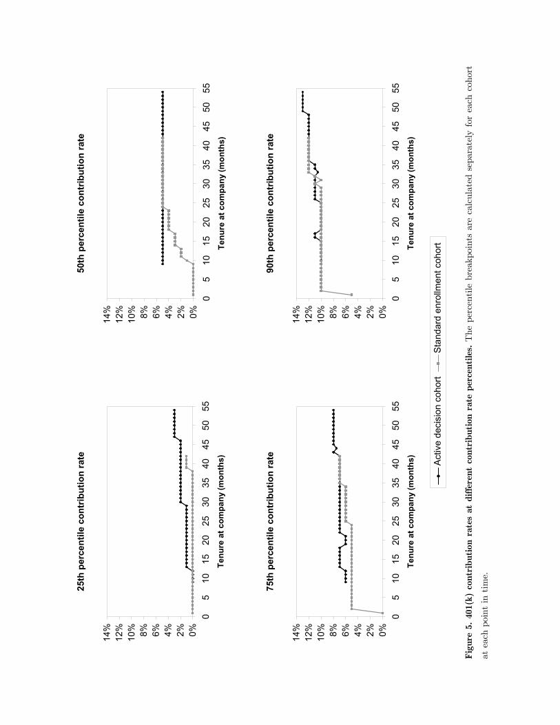
25th

per

cent

ile c

ontr

ibut

ion

rate

0%2%4%6%8%10%

12%

14%

05

1015

2025

3035

4045

5055

Tenu

re a

t com

pany

(mon

ths)

50

th p

erce

ntile

con

trib

utio

n ra

te

0%2%4%6%8%10%

12%

14%

05

1015

2025

3035

4045

5055

Tenu

re a

t com

pany

(mon

ths)

75th

per

cent

ile c

ontr

ibut

ion

rate

0%2%4%6%8%10%

12%

14%

05

1015

2025

3035

4045

5055

Tenu

re a

t com

pany

(mon

ths)

90

th p

erce

ntile

con

trib

utio

n ra

te

0%2%4%6%8%10%

12%

14%

05

1015

2025

3035

4045

5055

Tenu

re a

t com

pany

(mon

ths)

Fi

gure

5. 4

01(k

) co

ntri

butio

n ra

tes

at d

iffer

ent

cont

ribu

tion

rate

per

cent

iles.

The

per

cent

ile b

reak

poin

ts a

re c

alcu

late

d se

para

tely

for

eac

h co

hort

at e

ach

poin

t in

tim

e.

Act

ive

deci

sion

coh

ort

Sta

ndar

d en

rollm

ent c

ohor

t

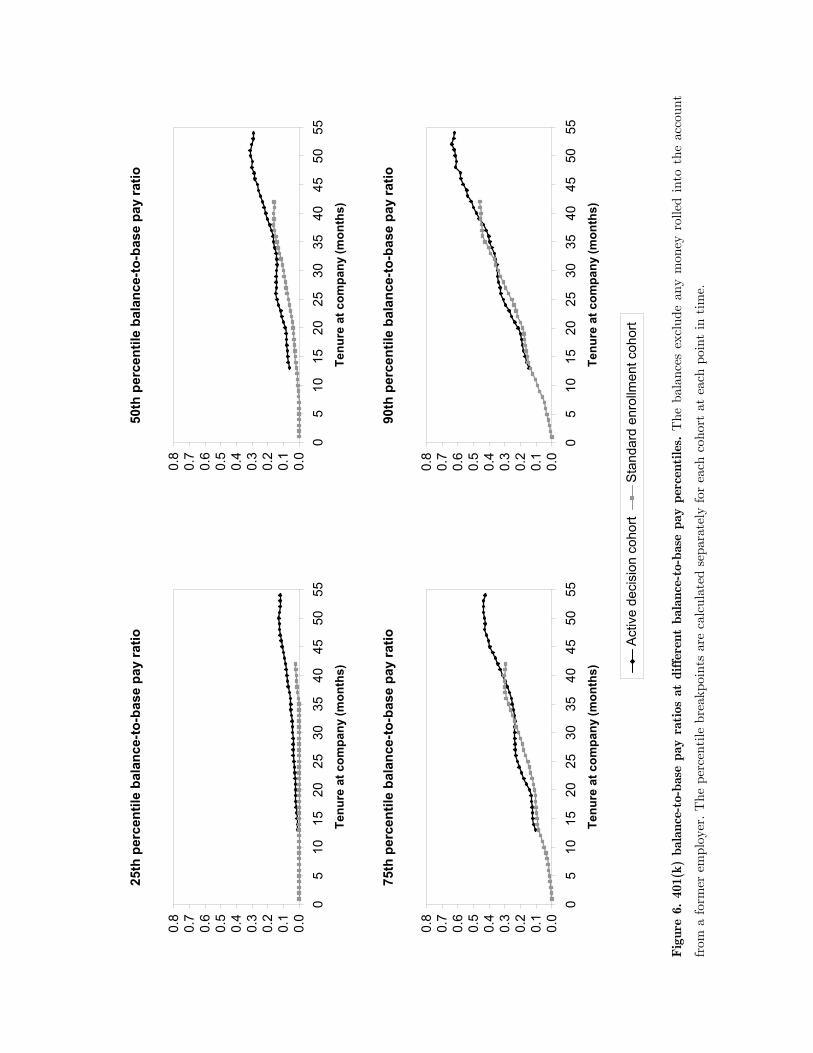
25th

per

cent

ile b

alan

ce-to

-bas

e pa

y ra

tio

0.0

0.1

0.2

0.3

0.4

0.5

0.6

0.7

0.8

05

1015

2025

3035

4045

5055

Tenu

re a

t com

pany

(mon

ths)

50

th p

erce

ntile

bal

ance

-to-b

ase

pay

ratio

0.0

0.1

0.2

0.3

0.4

0.5

0.6

0.7

0.8

05

1015

2025

3035

4045

5055

Tenu

re a

t com

pany

(mon

ths)

75th

per

cent

ile b

alan

ce-to

-bas

e pa

y ra

tio

0.0

0.1

0.2

0.3

0.4

0.5

0.6

0.7

0.8

05

1015

2025

3035

4045

5055

Tenu

re a

t com

pany

(mon

ths)

90

th p

erce

ntile

bal

ance

-to-b

ase

pay

ratio

0.0

0.1

0.2

0.3

0.4

0.5

0.6

0.7

0.8

05

1015

2025

3035

4045

5055

Tenu

re a

t com

pany

(mon

ths)

Fi

gure

6.

401(

k) b

alan

ce-t

o-ba

se p

ay r

atio

s at

diff

eren

t ba

lanc

e-to

-bas

e pa

y pe

rcen

tiles

. T

he b

alan

ces

excl

ude

any

mon

ey r

olle

d in

to t

he a

ccou

nt

from

a fo

rmer

em

ploy

er. T

he p

erce

ntile

bre

akpo

ints

are

cal

cula

ted

sepa

rate

ly for

eac

h co

hort

at

each

poi

nt in

tim

e.

Act

ive

deci

sion

coh

ort

Sta

ndar

d en

rollm

ent c

ohor

t

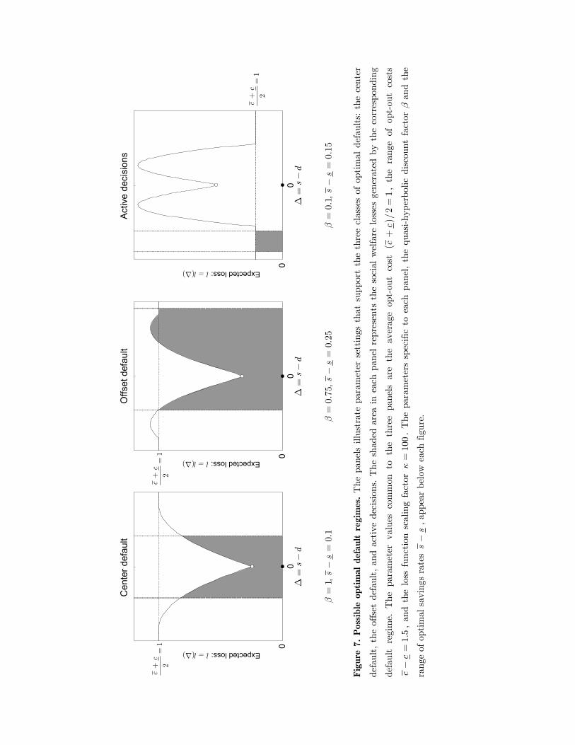
12

cc

+=

Cen

ter d

efau

ltO

ffset

def

ault

Act

ive

deci

sion

s

00

00

00

1,0.

1

sd

ss

β

∆=−

=−=

0.75

,0.

25

sd

ss

β

∆=−

=−=

0.1,

0.15

sd

ss

β

∆=−

=−=

Expected loss: l = l(∆)

Expected loss: l = l(∆)

Expected loss: l = l(∆)

12

cc

+=

12

cc

+=

Figu

re 7

. Pos

sible

opt

imal

def

ault

regi

mes

. The

pan

els

illus

trat

e pa

ram

eter

set

ting

s th

at s

uppo

rt t

he t

hree

cla

sses

of

opti

mal

def

aults:

the

cen

ter

defa

ult,

the

offs

et d

efau

lt, an

d ac

tive

dec

isio

ns. T

he s

hade

d ar

ea in

each

pan

el r

epre

sent

s th

e so

cial

wel

fare

los

ses

gene

rate

d by

the

cor

resp

ondi

ng

defa

ult

regi

me.

The

par

amet

er v

alue

s co

mm

on t

o th

e th

ree

pane

ls a

re t

he a

vera

ge o

pt-o

ut c

ost (

)/2

1c

c+

=,

the

rang

e of

opt

-out

cos

ts

1.5

cc−=

, an

d th

e lo

ss f

unct

ion

scal

ing

fact

or

. T

he p

aram

eter

s sp

ecifi

c to

eac

h pa

nel,

the

quas

i-hyp

erbo

lic d

isco

unt

fact

or β

and

the

rang

e of

opt

imal

sav

ings

rat

es

100

κ=

s−

s, a

ppea

r be

low

eac

h fig

ure.

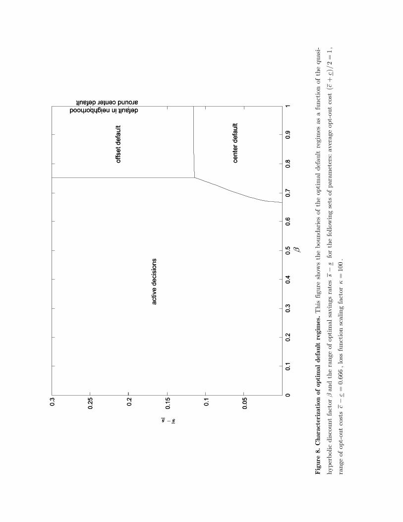
ss−

()/

21

cc+

=10

0κ=

activ

e de

cisi

ons

offs

et d

efau

lt

cent

er d

efau

lt

default in neighboraround center de

.30.

40.

50.

60.

70.

80.

91

β

activ

e de

cisi

ons

offs

et d

efau

lt

cent

er d

efau

lt

default in neighboraround center de

.30.

40.

50.

60.

70.

80.

91

β

Figu

re 8

. Cha

ract

eriz

atio

n of

opt

imal

def

ault

regi

mes

. Thi

s fig

ure

show

s th

e bo

unda

ries

of

the

optim

al d

efau

lt r

egim

es a

s a

func

tion

of

the

quas

i-

hype

rbol

ic d

isco

unt

fact

or β

and

the

ran

ge o

f op

tim

al s

avin

gs r

ates

for

the

fol

low

ing

sets

of pa

ram

eter

s: a

vera

ge o

pt-o

ut c

ost

,

rang

e of

opt

-out

cos

ts

, los

s fu

nction

sca

ling

fact

or

.

hoodfault

0.050.1

0.150.2

0.250.3

00.

10.

20

s�s

hoodfault

0.050.1

0.150.2

0.250.3

00.

10.

20

s�s s�s

0.66

6c

c−=