NBER WORKING PAPER SERIES

ON THE CONSEQUENCES OF DEMOGRAPHIC CHANGEFOR RATES OF RETURNS TO CAPITAL, AND THE

DISTRIBUTION OF WEALTH AND WELFARE

Dirk KruegerAlexander Ludwig

Working Paper 12453http://www.nber.org/papers/w12453

NATIONAL BUREAU OF ECONOMIC RESEARCH1050 Massachusetts Avenue

Cambridge, MA 02138August 2006

We thank participants of seminars at the LSE, Ente Einaudi, Koc, MEA, the 2005 Cleveland FEDInternational Macroeconomics conference, the 2006 Carnegie Rochester conference, the 2006 SED Meetingsand the 12th Dubrovnik Economic Conference for many useful comments. We are especially indebted to ourdiscussant Ayse Imrohoroglu for many helpful suggestions and comments. The authors can be reached atdirk.krueger@wiwi.uni-frankfurt.de and alexander.ludwig@mea.uni-mannheim.de. This paper was preparedfor the Spring 2006 Carnegie-Rochester Conference on Public Policy. The views expressed herein are thoseof the author(s) and do not necessarily reflect the views of the National Bureau of Economic Research.

©2006 by Dirk Krueger and Alexander Ludwig. All rights reserved. Short sections of text, not to exceed twoparagraphs, may be quoted without explicit permission provided that full credit, including © notice, is givento the source.

On the Consequences of Demographic Change for Rates of Returns to Capital, and theDistribution of Wealth and WelfareDirk Krueger and Alexander LudwigNBER Working Paper No. 12453August 2006JEL No. C68, D33, E17, E25

ABSTRACT

This paper employs a multi-country large scale Overlapping Generations model with uninsurablelabor productivity and mortality risk to quantify the impact of the demographic transition towardsan older population in industrialized countries on world-wide rates of return, international capitalflows and the distribution of wealth and welfare in the OECD. We find that for the U.S. as an openeconomy, rates of return are predicted to decline by 86 basis points between 2005 and 2080 andwages increase by about 4.1%. If the U.S. were a closed economy, rates of return would decline andwages increase by less. This is due to the fact that other regions in the OECD will age even morerapidly; therefore the U.S. is "importing" the more severe demographic transition from the rest ofthe OECD in the form of larger factor price changes. In terms of welfare, our model suggests thatyoung agents with little assets and currently low labor productivity gain, up to 1% in consumption,from higher wages associated with population aging. Older, asset-rich households tend to lose,because of the predicted decline in real returns to capital.

Dirk KruegerJohann Wolfgang Goethe University Frankurt-am-MainMertonstrasse 17, PF 8160054 Frankfurt-am-MainGERMANYand NBERdirk.krueger@wiwi.uni-frankfurt.de

Alexander LudwigMannheim Research Institute for the Economics of Aging, MEAUniversity of MannheimL13, 1768131 MannheimGERMANYludwig@mea.uni-mannheim.de

1 IntroductionIn all major industrialized countries the population is aging, over time reducingthe fraction of the population in working age. This process is driven by fallingmortality rates followed by a decline in birth rates, which reduces populationgrowth rates (and even turn them negative in some countries). While demo-graphic change occurs in all countries in the world, extent and timing differsubstantially. Europe and some Asian countries have almost passed the closingstages of the demographic transition process while Latin America and Africaare only at the beginning (Bloom and Williamson, 1998; United Nations, 2002).

2000 2010 2020 2030 2040 2050 2060 2070 2080−0.01

−0.005

0

0.005

0.01

0.015

0.02

0.025

0.03

Year

po

pg

r

population growth rate

USEuropean UnionRest OECDRest World

Figure 1: Evolution of the Population Growth Rate in 4 Regions

Figure 1, based on UN population projections, illustrates the differentialimpact of demographic change on population growth rates (defined here as thegrowth rate of the adult population) for the period 2000-2080 for four regions ofthe world that comprise the entire world: the U.S., the European Union (EU),the rest of the OECD (ROECD) and the rest of the world (ROW). Populationgrowth rates are predicted to decline in all regions, but are positive in the U.S.and in the ROW region throughout the 21st century, whereas they fall below zeroin the EU in about 2016 and in the ROECD in about 2042. As a consequence,the population in the EU (the ROECD) starts shrinking in about 2016 (2042),

2

whereas the population in the other two regions continues to increase.Figure 2 shows the impact of demographic change on working-age population

ratios - the ratio of the working-age population (of age 20-64) to the total adultpopulation (of age 20-95). This indicator, which will turn out to be crucialin our analysis, illustrates that the EU is the oldest, whereas the ROW is theyoungest region in terms of the relative size of the working-age population.The United States and the rest of the OECD region initially have the samelevel of working-age population ratios, but the dynamics of demographic changediffer substantially in the U.S. relative to the other regions. While working-age population ratios decrease across all regions, the speed of this decreasesignificantly slows down for the U.S. in about 2030.

2000 2010 2020 2030 2040 2050 2060 2070 20800.6

0.65

0.7

0.75

0.8

0.85

Year

wap

r

working age population ratio

USEuropean UnionRest OECDRest World

Figure 2: Evolution of Working Age to Population Ratios in 4 Regions

What are the welfare consequences of living in a world where the populationis aging rapidly? First, individuals live longer lives and tend to have fewerchildren, which are the underlying reasons of aging populations. The welfareeffects of these changes are hard to quantify. Second, due to changes in thepopulation structure, aggregate labor supply and aggregate savings is bound tochange, with ensuing changes in factor prices for labor and capital. Specifically,labor is expected to be scarce, relative to capital, with an ensuing increase inreal wages and decline in the real return on capital. The primary objective ofthis paper is to quantify the distributional and welfare consequences from this

3

second, general equilibrium effect of the demographic changes around the world.To this end, we use demographic projections from the United Nations, to-

gether with a large scale Overlapping Generations Model pioneered by Auerbachand Kotlikoff (1987). We extend the model to a multi-country version, as inBörsch-Supan et al. (2006), among many others, and also enrich the model byuninsurable idiosyncratic uncertainty, as in Imrohoroglu et al. (1995), Imro-horoglu et al. (1999), Conesa and Krueger (1999) and others. Both extensionsare necessary for the question we want to address. First, uninsurable idio-syncratic uncertainty will endogenously give rise to some agents deriving mostof their income from returns to capital, while the income of others is mainlycomposed of labor income. Abstracting from this heterogeneity does not allowa meaningful analysis of the distributional consequences of changes in factorprices. This feature also adds a precautionary savings motive to the standardlife-cycle savings motive of households, which makes life cycle savings profilesgenerated by the model more realistic. Second, in light of potential differencesin the evolution of the age distribution of households across regions, it is impor-tant to allow for capital to flow across regions. In our model capital can freelyflow between different regions in the OECD (the U.S., the EU and the rest of theOECD). These capital flows may mitigate the decline in rates of return and theincrease in real wages one would expect in the U.S. if it were a closed economy.We find exactly the opposite. In the U.S. as an open economy, rates of return

are predicted to decline by 86 basis points between 2005 and 2080. If the U.S.were a closed economy, this decline would amount to only 79 basis points. Thisresult is due to the fact that other regions in the OECD will age even morerapidly. Therefore the U.S. is “importing” the more severe aging problem fromthese regions via a stronger increase in wages and a stronger decline in interestrates, relative to being a closed economy.In order to evaluate the welfare consequences of the demographic transition

we ask the following question: suppose a household economically born in 2005would live through the economic transition with changing factor prices inducedby the demographic change (but keeping its own survival probabilities constantat their 2005 values), how would its welfare have changed, relative to a situationwithout a demographic transition? We find that for young households with littleassets the increase in wages dominates the decline in rates of return. Abstractingfrom social security and its reform newborns in 2005 gain in the order of 0.6-0.9%in terms of lifetime consumption. Older, asset-rich individuals, on the otherhand, tend to lose because of the decline in interest rates. If the demographictransition, in addition, makes a reform of the social security system necessary,then falling benefits or increasing taxes reduce the welfare gains for newbornagents. An increase in the retirement age to 70, on the other hand, mitigatessome of these negative consequences.Our paper borrows model elements from, and contributes to, three strands

of the literature. Starting with Auerbach and Kotlikoff (1987) a vast numberof papers has used large-scale OLG models to analyze the transition path of aneconomy induced by a policy reform. Examples include social security reform(see e.g. Conesa and Krueger (1999)), fundamental tax reform (see e.g. Altig

4

et al. (2001), Conesa and Krueger (2005)) and many others.A second strand of the literature (often using the general methodology of

the first strand) has focused on the economic consequences of population agingin closed economies, often paying special attention to the adjustments requiredin the social security system due to demographic shifts. Important examplesinclude Huang et al. (1997), De Nardi et al. (1999), and, with respect to assetprices, Abel (2003).The contributions discussed so far assume that the economy under investi-

gation is closed to international capital flows. However, as the population agesat different pace in various regions of the world one would expect capital to flowacross these regions. The third strand of the literature our paper touches upontherefore is the large body of work in international macroeconomics studying thedirection, size, cause and consequences of international capital flows and currentaccount dynamics, reviewed comprehensively in Obstfeld and Rogoff (1995).Our paper is most closely related to work that combines these three strands of

the literature, by using the methodology of large scale OLG models to study theconsequences of demographic change in open economies. The work by Attanasioet al. (2006b) constructs a two region (the North and the South) OLG model tostudy the allocative and welfare consequences of different social security reformsin an open economy. Compared to their model, we include endogenous laborsupply and idiosyncratic income shocks. While we also have to take a standon how the social security system deals with the aging of the population, thesesocial security reforms are not in the center of our analysis whereas their paperfocuses on this issue. In Attanasio et al. (2006a) the authors quantify the directwelfare losses from demographic changes for the South region of their model,carrying out a similar thought experiment we do for the U.S..Similar to Attanasio et al. (2006b), but with a stronger focus on Europe or

the OECD, Börsch-Supan et al. (2006) and Fehr et al. (2005) investigate theimpact of population aging on the viability of the social security system andits reform. Building on earlier work by Brooks (2003) who employs a simplefour period OLG model, Henriksen (2002), Feroli (2003) and Domeij and Floden(2005) use large scale simulation models similar to Börsch-Supan et al. (2006)to explain historical capital flow data with changes in demographics, ratherthan, as we do, to study the (welfare and distributional) implications of futurechanges in demographics. Relative to this literature, we see the contribution ofour paper in evaluating the welfare consequences of the demographic transitionper se and not just the alternative social security reform scenarios, as well as inthe analysis of the distributional consequences of changing factor prices due topopulation aging.The paper is organized as follows. In the next section we construct a simple,

analytically tractable multi-country OLG model to isolate the key determinantsof international capital flows and the impact of changes in the demographicstructure on rates of return and capital flows. Section 3 contains the descrip-tion of our large scale simulation model. Section 4 discusses the calibration ofthe model and section 5 presents results for the benchmark model. In section 6we compare our results to what would be obtained in a closed economy model.

5

There we also disentangle the effects from changing fertility and mortality. Sec-tion 7 concludes, and separate appendices contain more detailed informationabout the demographic model underlying our simulations, as well as details ofthe computational strategy and calibration of the model.

2 A Simple ModelWe now construct a simple OLG model that is a special case of our quantitativemodel in the next section. We can characterize equilibria in this model ana-lytically, and are especially interested in the influence of demographic variablesand the size of the social security system on rates of return to capital and thedynamics of international capital flows. The results of this simple model willprovide some intuition for the quantitative results from the simulation model.In every country i there are Nt,i young households who live for two periods

and have preferences over consumption cyt,i, cot+1,i representable by the utility

functionlog(cyt,i) + β log(cot+1,i).

In the first period of their lives households work for a wage wt,i, and in thesecond period they retire and receive social security benefits bt+1,i, financed viapayroll taxes on labor income. Thus the budget constraints read as

cyt + st = (1− τ t,i)wt,i

cot+1 = (1 + rt+1)st + bt+1,i

where rt+1 is the real interest rate between period t and t + 1 and τ t,i is thesocial security tax rate in country i. We assume that capital flows freely acrosscountries, and thus the real interest rate is equalized across the world.The production function in each country is given by

Yt,i = Kαt,i (ZiAtNt,i)

1−α ,

where Zi is the country-specific technology level and At = (1+g)t is exogenously

growing productivity. Thus we allow for differences in technology levels acrosscountries, but not its growth rate. We further assume that capital depreciatesfully after its use in production.The production technology in each country is operated by a representative

firm that behaves competitively in product and factor markets. Profit maxi-mization of firms therefore implies that

1 + rt = αkα−1t

wt,i = (1− α)ZiAtkαt , (1)

where

kt = kt,i =Kt,i

ZiAtNt,i∀i

is the capital stock per efficiency unit of labor.

6

We assume that the social security system is a pure pay-as-you-go (PAYGO)system that balances the budget in every period. Therefore

τ t,iwt,iNt,i = bt,iNt−1,i.

Finally, market clearing in the world capital market requires that

Kt+1 =Xi

Kt+1,i =Xi

Nt,ist,i.

2.1 Analysis

Equilibria in this model can be characterized analytically. To do so we firstsolve the household problem and then aggregate across households (countries).

2.1.1 Optimal Household Savings Behavior

Optimal saving of the young in country i are given as

st,i =β

1 + βwt,i(1− τ t,i)−

bt+1,i(1 + β)(1 + rt+1)

. (2)

The budget constraint of the social security system implies that

bt,i =Nt,i

Nt−1,iwt,iτ t,i = γNt,iwt,iτ t,i,

where γNt,i is the gross growth rate of the young cohort in country i betweenperiod t − 1 and t. It also measures the working age to population ratio (thehigher is γNt,i, the higher is that ratio)

1, which allows us to map the predictionsof this model to the data plotted in figure 2. Using the expression for benefitsand substituting out for wages and interest rates from (1) in (2) yields

st,i =β(1− τ t,i)(1− α)

1 + βZiAtk

αt −

γNt+1,iτ t+1,i(1− α)

(1 + β)αZiAt+1kt+1. (3)

1The population of a country i at time t is given by

Popt,i = Nt,i +Nt−1,i

and the working age to population ratio is given by

waprt,i =Nt,i

Popt,i.

Then we can easily compute the growth rate of the population as

γPopt,i =Popt+1,i

Popt,i=

1 + γNt,i

1 + 1γNt−1,i

.

In a balanced growth path γPopi = γNi and furthermore wapri = 11+ 1

γNi

. Thus γNi is a measure

both of the population growth rate as well as the working age to population ratio.

7

2.1.2 Aggregation

For further reference, define by Nt =P

i ZiNt,i the efficiency weighted world

population, by θt,i =ZiNt,i

Nt=

Nt,i

Ntthe relative share of the efficiency-weighted

population in country i and by γNt =Nt

Nt−1=P

i θt,iγNt,i the growth rate of the

aggregate (world) efficiency weighted population.The capital market clearing condition readsX

i

st,iNt,i =Xi

Kt+1,i = kt+1Xi

ZiAt+1Nt+1,i = kt+1At+1Nt+1 (4)

Aggregating household savings decisions across countries yields, from (3):Xi

st,iNt,i =(1− α)βAtk

αt

1 + β

Xi

(1−τ t,i)ZiNt,i−(1− α)At+1kt+1

(1 + β)α

Xi

ZiNt+1,iτ t+1,i

Using this in (4) and simplifying yields

kt+1 = σtkαt (5)

where

σt =α(1− α)β(1− τat )

γNt+1γA¡α(1 + β) + (1− α)τat+1

¢is the fraction of output per effective worker that is saved. Here τat =

Pi τ t,iθt,i

denotes the average social security contribution rate in the world and γA = 1+gis the growth rate of technology. Equation (5), as a function of the policy anddemographic parameters of the model, describes the dynamics of the aggregatecapital stock, given the initial condition k0.

2 Since, from the firms’ first ordercondition, interest rates are given by

1 + rt = αkα−1t

the dynamics of the real interest rate are given by

1 + rt+1 =

µα

σt

¶1−α(1 + rt)

α (6)

with initial condition 1 + r0 = αkα−10 .

2.1.3 Balanced Growth Path Analysis

A balanced growth path (BGP) is characterized by a constant effective capitalstock k = σ

11−α where

σ =α(1− α)β(1− τa)

γNγA (α(1 + β) + (1− α)τa)

2Explicitly, k0 = i s−1,iN−1,iA0 i ZiN0,i

where s−1,iN−1,i denotes total assets held by the initial

old generation in country i.

8

Evidently, normalized and productivity de-trended per capita output in countryi is then given by

Yt,iZiAt(Nt,i +Nt−1,i)

=σ

α1−α γNi1 + γNi

. (7)

To gain further intuition it is instructive to relate rates of return to savingsrates along a BGP. World saving (equal to investment) is given by

St = Kt+1 −Kt

and along a BGP capital grows at a constant rate γAγN , so that

St = [γAγN − 1]Kt

Thus the world-wide saving (investment) rate along the BGP is given by

srt =StYt= [γAγN − 1]Kt

Yt= [γAγN − 1] ktAt

Pi ZiNt,i

kαt At

Pi ZiNt,i

= [γAγN − 1]k1−α = [γAγN − 1] ∗ α

1 + r= sr

or

1 + r =α[γAγN − 1]

sr(8)

which shows that interest rates and savings rates are negatively related: a highersavings rate, ceteris paribus, increases the supply of capital and thus depressesthe rate of return. Of course both the interest rate and the world savings rateare endogenous, and functions of the underlying parameters. It directly followsthat along the BGP

sr = [1− (γNγA)−1] α(1− α)β(1− τa)

(α(1 + β) + (1− α)τa)(9)

1 + r = γAγN(α(1 + β) + (1− α)τa)

(1− α)β(1− τa)(10)

Furthermore, we can characterize international capital flows and the currentaccount. Define savings and investment rates as well as the current account (asfraction of output) in country i as

srt,i =At+1,i −At,i

Yt,i

irt,i =Kt+1,i −Kt,i

Yt,icat,i = srt,i − irt,i

9

Along a BGP we can determine, after some tedious algebra,

iri = [1− (γAγNi )−1]γNi α(1− α)β(1− τa)

γN (α(1 + β) + (1− α)τa)(11)

sri = [1− (γAγNi )−1]∙β(1− α)(1− τ i)

1 + β− β(1− α)τ i

(1 + β)

γNi (1− α)(1− τa)

γN (α(1 + β) + (1− α)τa)

¸(12)

cai = [1− (γAγNi )−1]β(1− α)(1− τ i)

1 + β

∙1− γNi (1− τa) (α(1 + β) + (1− α)τ i)

γN (1− τ i) (α(1 + β) + (1− α)τa)

¸(13)

Finally, net foreign asset positions and the current account in the BGP arerelated according to

CAt,i = Ft+1,i − Ft,i = [1− (γAγNi )−1]Ft+1,i

cai =CAt,i

Yt,i= [1− (γAγNi )−1]fi where fi =

Ft+1,iYt,i

and thus

fi =β(1− α)(1− τ i)

1 + β

∙1− γNi (1− τa)(α(1 + β) + (1− α)τ i)

γN (1− τ i)(α(1 + β) + (1− α)τa)

¸(14)

2.2 Qualitative Predictions from the Simple Model

In this section we illustrate, using equations (8)-(14), how an aging population(as captured by a decline in γN ), or an increase in social security contribu-tion rates induced by demographic changes (as captured by an increase in τ)affects world-wide rates of return, country-specific per capita output, savingsand investment rates as well as the current account and the net foreign assetposition.

2.2.1 Rates of Return

First we determine the consequences of a decline in the working age to popu-lation ratio in the BGP. From equation (10) we immediately see that despitethe fact that the interest rate and the savings rate are negatively related (seeequation (8)), a decline in the working age to population ratio γN leads to botha decline in the rate of return r and in the saving rate sr. What is the intu-ition? A reduction of γN reduces the number of young people relative to oldpeople. Since savings is only done by the young, the savings rate in the economydeclines. This makes capital scarce and, ceteris paribus, increases r (see equa-tion 8). But there is the direct effect on the interest rate r: a reduction of γN

reduces labor supply tomorrow (as there are fewer young), making labor scarcerelative to capital. In the simple model of this section this effect is theoreticallyshown to dominate, and hence r falls.

10

Equation (10) shows another potential, indirect effect from population agingon the interest rate that stems from the social security system. An increase inthe (world average) social security contribution rate τa, by reducing privatesavings rates, is predicted to drive up rates of return. If policy makers wantto keep social security benefits stable despite an aging population, an increasein contribution rates is required. Because this, ceteris paribus, drives up futurerates of return, the adjustment of τa mitigates or even dominates the directeffect of population aging via a decline of γN , as also highlighted by Fehr et al.(2005).3

To summarize, a decline in the world-wide working age to population ratioleads to a decline in rates of return to capital, as long as social security contribu-tion rates are held constant (and thus benefits shrink). If, however, contributionrates are raised in addition, to keep social security benefits stable, the predicteddecline in returns is smaller, or returns may even increase. Quantitative work isneeded to measure the relative strength of these effects, something we will turnto in the next sections of this paper.

2.2.2 Per Capita Output

The simple decomposition in equation (7) illustrates the various channels throughwhich demographic change affects per capita output in country i. As the mostdirect effect, a decrease in the working age to population ratio in country i asmeasured by γNi leads to a decrease of the overall population which means thatthe existing resources have to be shared by less people. However, the decrease ofthe working age to population ratio also directly reduces the labor force whichsuppresses overall output. An additional positive effect on per capita outputstems from capital depending because decreasing γNi , through its effect on γN ,leads to an increase of σ and thereby to an increase of the long-run capital cap-ital stock per efficient worker, k. Finally, an additional indirect effect alreadyfamiliar from the above discussion on rates of return emanates from increasesin contribution rates, τa, if social security benefit levels were to be maintained.This harms capital accumulation. Again, quantitative work is needed to mea-sure the relative strengths of these various effects.

2.2.3 Net Foreign Asset Positions

Finally we want to deduce the implications of the simple model for the cur-rent account and net foreign asset positions across countries. First we observefrom equations (13) and (14) that if all countries are identical with respect totheir demographic structure and size of the social security system, then the cur-rent account and the net foreign asset positions are equal to zero. Thus the

3The preceding analysis also holds outside the balanced growth path, as equation (6) shows.Since kt and hence rt is predetermined, we observe from equation (6) that the response ofrt+1 depends negatively on the world saving rate σt, which is itself a negative function of theefficiency-weighted population growth rate γNt+1 between period t and t + 1 and a positivefunction of the social security contribution rate τat+1. The same qualitative predictions as inthe BGP follow.

11

only reason for capital to flow across countries in our model are differences indemographics and in the size of the social security system.What are the consequences of a reduction in the working age to population

ratio γNi , abstracting from social security (that is, setting τ i = τa = 0)?4 Weobserve from equations (11) and (12) that both investment as well as savingsrates decline with a decrease in γNi , for the same reason as the world savingsrate decreased above. What happens to the current account and the net foreignasset position of country i depends on whether it is aging faster or slower thanthe rest of the world. If all countries age at the same speed (the ratio γNi /γ

N

remains unchanged) then the net foreign asset position remains unchanged andthe current account declines in absolute value. If, on the other hand, countryi ages faster than the rest (γNi /γ

N decreases), then its net foreign asset posi-tion and its current account increase: capital flows from regions that are agingfaster to regions that are aging slower. Notice that the term γNi /γ

N appearsin equation (11) but not in equation (12) which illustrates that the strengthof demographic change in country i relative to the other world regions directlyaffects investment rates but not savings rates.Finally, if all countries have identical working age to population ratios (γNi /γ

N

remains at 1), but country i increases its social security contribution rate τ i then(assuming for simplicity τa = 0) we observe from equations (11)-(14) that coun-try i’s investment rate remains unchanged, its private savings rate sri declines,and with it the current account and the net foreign asset position. We will lateruse these qualitative predictions from the simple model to interpret our resultsfrom the quantitative model to which we turn next.

3 The Quantitative ModelIn this section we describe the quantitative model we use to evaluate the conse-quences of demographic changes for international capital flows, returns to capitaland wages, as well as the welfare consequences emanating from these changes.In our quantitative work we consider three countries/regions: the United States(U.S.), the European Union (EU) and the rest of the OECD (ROECD).

3.1 Demographics

The demographic evolution in our model is taken as exogenous (i.e. we do notmodel fertility, mortality or migration) and is the main driving force of ourmodel. Households start their economic life at age 20, retire at age 65 and liveat most until age 95. Since we do not model childhood of a household explicitly,we denote its twentieth year of life by j = 0, its retirement age by jr = 45 andthe terminal age of life by J = 75. Households face an idiosyncratic, time- andcountry-dependent (conditional) probability to survive from age j to age j + 1,which we denote by st,j,i.

4Most of these results can be shown under the less restrictive assumption that τ i = τα 6= 0.

12

For each country i we have data or forecasts for populations of model agej ∈ {0, . . . , 75} in years 1950, . . . , 2300. From now on we denote year 1950 asour base year t = 0 and year 2300 as the final period T and the demographicdata for periods t ∈ {0, . . . , T} by Nt,j,i. For simplicity, we assume that allmigration takes place at or before age j = 0 in the model (age 20 in the data),so that we can treat migrants and agents born inside the country of interestsymmetrically.

3.2 Technology

In each country the single consumption good is being produced according to astandard neoclassical production function

Yt,i = ZiKαt,i (AtLt,i)

1−α ,

where Yt,i is output in country i at date t, Kt,i and Lt,i are capital and la-bor inputs and At is total labor productivity, growing at a constant countryindependent rate g. The scaling parameters Zi control relative total factor pro-ductivities across countries, whereas the parameter α measures the capital shareand is assumed to be constant over time and across countries. In each countrycapital used in production depreciates at a common rate δ. Since productiontakes place with a constant-returns to scale production function and since weassume perfect competition, the number of firms is indeterminate in equilib-rium and, without loss of generality, we assume that a single representative firmoperates within each country.

3.3 Endowments and Preferences

Households value consumption and leisure over the life cycle {cj , 1−lj} accordingto a standard time-separable utility function

E

⎧⎨⎩JXj=0

βju(cj , 1− lj)

⎫⎬⎭ ,

where β is the raw time discount factor and expectations are taken over idio-syncratic mortality shocks and stochastic labor productivity. In particular, theexpectations operator E encompasses the survival probabilities st,j,i.Households are heterogenous with respect to age, a deterministic earnings

potential and stochastic labor productivity. These sources of heterogeneity affecta household’s labor productivity which is given by

θkεjη.

First, households labor productivity differs according to their age: εj denotesaverage age-specific productivity of cohort j. Second, each household belongsto a particular group k ∈ {1, . . . ,K} that shares the same average productivity

13

θk. Differences in groups stand in for differences in education or ability, char-acteristics that are fixed at entry into the labor market and affect a group’srelative wage. We introduce these differences in order to generate part of thecross-sectional income and thus wealth dispersion that does not come from ourlast source of heterogeneity, idiosyncratic productivity shocks. Lastly, a house-hold’s labor productivity is affected by an idiosyncratic shock, η ∈ {1, . . . , E}that follows a time-invariant Markov chain with transition probabilities

π(η0|η) > 0.

We denote by Π the unique invariant distribution associated with π.

3.4 Government Policies

The government collects assets of households that die before age J and redis-tributes them in a lump-sum fashion among the citizens of the country as ac-cidental bequests, ht,i (inheritances). Furthermore, we explore how our resultsare affected by the presence and the design of a pure pay-as-you-go public pen-sion system, whose taxes and benefits have to be adjusted to the demographicchanges in each country. The social security system is modelled as follows. Onthe revenue side, households pay a flat payroll tax rate τ t,i on their labor earn-ings. Retired households receive benefits, bt,k,i, that are assumed to dependon the household type, θk, but are independent of the history of idiosyncraticproductivity shocks. Pension benefits are therefore given by

bt,k,i = ρt,iθk(1− τ t,i)wt,i, (15)

where ρt,i is the pension system’s net replacement rate.We assume that the budget of the pension system is balanced at all times

such that taxes and benefits are related by

τ t,iwt,iLt,i =Xk

bt,k,iXj≥jr

Nt,j,k,i, (16)

where Nt,j,k,i denotes the population in country i at time t of age j and type k.In our results section we distinguish between three different scenarios for the

future evolution of the social security system, one in which taxes are held con-stant and replacement rates adjust accordingly, and vice versa. A third scenariomodels an increase in the retirement age (and in addition adjusts benefits, ifneeded, to assure budget balance). The results from the simple model abovesuggests that our results will be significantly affected by the modelling choicefor social security.

3.5 Market Structure

In each period there are spot markets for the consumption good, for labor andfor capital services. While the labor market is a national market where labor

14

demand and labor supply are equalized country by country, the markets for theconsumption good and capital services are international where goods and capitalflow freely, and without any transaction costs, between countries. The supply ofcapital for production stems from households in all countries who purchase theseassets in order to save for retirement and to smooth idiosyncratic productivityshocks. As sensitivity analysis, we explore how countries would be affected bytheir demographic changes if they were closed economies where capital stocksand accumulated assets coincide by definition.

3.6 Equilibrium

Individual households, at the beginning of period t are indexed by their age j,their group k, their country of origin i, their idiosyncratic productivity chock η,and their asset holdings a. Thus their maximization problem reads as

W (t, j, k, i, η, a) (17)

= maxc,a0,1−l

{u(c, 1− l) + βst,j,iXη0

π(η0|η)W (t+ 1, j + 1, k, i, η0, a0)}

s.t. c+ a0 =

((1− τ t,i)wt,iθkεjηl + (1 + rt)(a+ ht,i) for j < jr

bt,k,i + (1 + rt)(a+ ht,i) for j ≥ jr

a0, c ≥ 0 and l ∈ [0, 1]·

Here wt,i is the wage rate per efficiency unit of labor and rt is the real interestrate. We denote the cross-sectional measure of households in country i at timet by Φt,i. We can then define a competitive equilibrium as follows.

Definition 1 Given initial capital stocks and measures {K0,i,Φ0,i}i∈I , a com-petitive equilibrium are sequences of individual functions for the household, {W (t, ·), c(t, ·), l(t, ·), a0(t, ·)}∞t=0,sequences of production plans for firms {Lt,i,Kt,i}∞t=0,i∈I , policies {τ t,i, ρt,i, bt,i}∞t=0,i∈I ,prices {wt,i, rt}∞t=0,i∈I , transfers {ht,i}∞t=0,i∈I and measures {Φt,i}∞t=0,i∈I suchthat

1. Given prices, transfers and initial conditions, W (t, ·) solves equation (17),and c(t, ·), l(t, ·), a0(t, ·) are the associated policy functions.

2. Interest rates and wages satisfy

rt = αZi

µKt,i

AtLt,i

¶α−1− δ

wt,i = (1− α)ZiAt

µKt,i

AtLt,i

¶α.

3. Transfers are given by

ht+1,i =

R(1− st,j,i)a

0(t, j, k, i, η, a)Φt,i(dj × dk × dη × da)RΦt+1,i(dj × dk × dη × da)

(18)

15

4. Government policies satisfy (15) and (16) in every period.

5. Markets clear in all t, i

Lt,i =

Zθkεjηl(t, j, k, i, η, a)Φt,i(dj × dk × dη × da) for all i

IXi=1

Kt+1,i =IXi=1

Za0(t, j, k, i, η, a)Φt,i(dj × dk × dη × da) for all i

IXi=1

Zc(t, j, k, i, η, a)Φt,i(dj × dk × dη × da) +

IXi=1

Kt+1,i

=IXi=1

At,iKαt,iL

1−αt,i + (1− δ)

IXi=1

Kt,i for all i.

6. The cross-sectional measures Φt,i evolve as

Φt+1,i(J×K×E×A) =Z

Pt,i((j, k, η, a),J×K×E×A)Φt,i(dj×dk×dη×da)

for all sets, J , K, E , A, where the Markov transition functions Pt,i aregiven by

Pt,i((j, k, η, a),J×K×E×A) =

⎧⎨⎩ π(η, E)st,j,iif a0(t, j, k, i, η, a) ∈ A

k ∈ K, j + 1 ∈ J0 else

and for newborns

Φt+1,i({1} × K × E ×A) = Nt+1,0,i ·½Π(E) if 0 ∈ A0 else

.

Definition 2 A stationary equilibrium is a competitive equilibrium in which allindividual functions are constant over time and all aggregate variables grow ata constant rate.

3.7 Thought Experiment and Computation

We take as exogenous driving process a time-varying demographic structure inall regions under consideration. We allow country-specific survival, fertility andmigration rates to change over time, inducing a demographic transition froman initial distribution towards a final steady state population distribution thatarises once all changes in these rates have been completed and the populationstructure has settled down to its new steady state. Induced by this transitionof the population structure is a transition path of the economies of the model,both in terms of aggregate variables as well as cross-sectional distributions ofwealth and welfare. Summary measures of these changes will provide us with

16

answers as to how the changes in the demographic structure of the economy, bychanging returns to capital and wages, impact the distribution of welfare.We start computations in year 1950 assuming an artificial initial steady state.

We then use data for a calibration period, 1950-2004, to determine several struc-tural model parameters (see section 4). We then compute the model equilibriumfrom 1950 to 2300 (when the new steady state is assumed and verified to bereached) and report simulation results for the main projection period of inter-est, from 2005 to 2080. For given structural model parameters we solve forthe equilibrium using a modification of the familiar Gauss-Seidel algorithm (seeLudwig, 2006). Throughout we take as length of the period one year. AppendixB contains a detailed description of our computational procedure.

4 CalibrationIn this section we discuss our specification of the model parameters. We need tochoose parameters governing the demographic transition, the production tech-nology, endowments and preferences, and the social security policy.

4.1 Demographics

Our demographic processes are based on the United Nations world populationprojections (United Nations, 2001). These numbers determine both the idiosyn-cratic survival probabilities as well as the relative sizes of total populations inthe regions in all time periods under consideration. Figures 1 and 2 in the intro-duction summarized the main stylized facts from these population figures, andappendix A describes in detail the methodology underlying our demographicprojections.

4.2 Technology

We restrict the capital share parameter, α, the growth rate of labor produc-tivity, g, and the depreciation rate, δ, to be constant across all regions underconsideration, whereas we allow technology levels Zi to differ across regions.The parameters characterizing production technologies in different countriescan therefore be collected as

ΨPS = [α, g, δ, Z1, Z2, Z3]0 .

We estimate parameters α, g and δ using U.S. NIPA data for a sample periodof 1960-2004, set Z1 = 1 and estimate Z2, Z3 taking data on relative laborproductivity across regions. A more detailed description of our approach isgiven in appendix B.3. Table I summarizes the resulting parameter estimates.

17

Table I: Technology ParametersParameter U.S. EU ROECDCapital Share α 0.33Growth Rate of Technology g 0.018Depreciation Rate δ 0.04Total Factor Productivity Zi 1.0 0.88 0.65

4.3 Endowments and Preferences

Households start their life with zero assets and are endowed with one unit of timeper period. Labor productivity is given by the product of three components,a deterministic age component εj , a deterministic group component θk and astochastic idiosyncratic component η.The age-productivity profile {εj}Jj=1 is taken from Hansen (1993) and gener-

ates an average life-cycle wage profile consistent with U.S. data. In experimentswhere we extend the retirement age we linearly extrapolate the efficiency profilebeyond age 65.Conditional on age, the natural logarithm of wages is given by

log(θk) + log(η).

We choose the number of groups to be K = 2 and let groups be of equal size.We choose {θ1, θ2} such that average-group productivity is equal to 1 and thevariance of implied labor incomes of entrants to the labor market coincideswith that reported by Storesletten et al. (2004). This requires θ1 = 0.57 andθ2 = 1.43. For the idiosyncratic part of labor productivity we use a 2 stateMarkov chain with annual persistence of 0.98 and implied conditional varianceof 8%, again motivated by the findings of Storesletten et al. (2004).We assume that the period utility function is of the familiar CRRA form

given by

u(c, l) =1

1− σ

¡cωi(1− l)1−ωi

¢1−σ,

where σ denotes the coefficient of relative risk aversion and where ωi measuresthe importance of consumption, relative to leisure in each country. Differences inωi across countries allow us to match simulated hours worked to the actual dataseparately for each country. In addition we have to specify the time discountfactor of households which we restrict to be identical across countries.The preference parameters can accordingly be summarized as

ΨHS = [σ, β, ω1, ω2, ω3]0.

We assume σ = 1 such that utility is separable between consumption and leisure,and determine the value of the discount rate by matching the average simulatedcapital-output ratio to U.S. data for the period 1960-2004. The consumptionshare parameters ωi are estimated by matching simulated average hours workedin the regions of our model to the data. A more detailed description of our

18

methodology is given in appendix B.3. Table II summarizes the preferenceparameters for the version of our model where a pension system is present.5

Table II: Preference ParametersParameter U.S. EU ROECDCoefficient of RRA σ 1.0Time Discount Factor β 0.9378Consumption Share Parameter ωi 0.463 0.446 0.442

4.4 Social Security System

Our benchmark model contains no social security system. The version of themodel used most prominently in our welfare calculations contains the PAYGOsocial security system, uses historical data for social security tax rates in thethree regions of interest until 2004 and then freezes future contribution rates attheir 2004 levels. Benefits adjust to achieve budget balance. In the alternativescenario of fixed replacement rates we again use historical region-specific dataon contribution rates to back out constructed replacement rates until 2004 andthen fix replacement rates in the future to their 2004 values. Tax rates increaseto assure budget balance of the social security system.Data for calibrating the social security system are taken from various sources.

For the U.S., we calculate social security contribution rates from NIPA datataken from the BEA (Table 3.6). It is more difficult to obtain data for the otherworld regions. We proxy the time path of social security contribution rates byusing time path information on total labor costs taken from the BLS and scalethese data by social security contribution rates from the OECD for the otherregions of interest.

5 Results for the Benchmark ModelIn order to isolate the direct effects of demographic changes on returns to capital,international capital flows, and the distribution of wealth and welfare we firstabstract from social security. In section 5.5 we then quantify the additionaleffects that are implied by the adjustments of social security parameters todemographic change. In the benchmark scenario we also assume that capitalflows freely only between regions in the OECD, and we document in section 6.1how our results are affected if these regions would be closed economies.

5.1 Steady State Comparison

In order to obtain first sense for the impact of changes in demographics on theeconomy, table III compares the main economic aggregates between the initial

5For each alternative version of our model all household model parameters are recalibratedto match the same aggregate data described above. Estimated parameter values for thesealternative versions are similar to those reported in table II.

19

steady state in 1950 and the final steady state in 2300. Here l denotes averagehours worked per person in working age. The table, which displays percentagechanges between the new and the old steady state (for the interest rate andaverage hours percentage point differences are shown), documents a substantialdecline in real rates of return between the old steady state in 1950 and the newsteady state in 2300 by more than 300 basis points. Detrended real wages, onthe other hand, increase by 14%, resulting from substantial capital deepening.These findings are exactly what our simple model led us to expect. As thediscussion of equation (7) in the analysis of the simple model already showed, thelong run consequences for output (income) per capita are less clear. On the onehand, output per worker increases substantially (due to a shrinking population,capital deepening and slightly increased age-specific labor supply shares), but,on the other hand, the fraction of the population that works declines. Table IIIdemonstrates that detrended output per capita declines slightly in the long run,suggesting that the aging effect dominates the capital deepening effect.6

Table III: Steady State ComparisonVariable United States Eur. Union Rest OECDr −3.06% −3.06% −3.06%w 14.1% 14.1% 14.1%Y/N −2.23% −0.10% −5.8%l 5.4% 6.0% 4.1%

The effects documented in table III incorporate the entire demographic tran-sition. In our subsequent analysis we now zoom in on our main period of interest,the next 75 years. Since only a part of the dramatic aging of the populationfalls into this period we expect the same qualitative, but quantitatively smallereffects.

5.2 Dynamics of Aggregate Statistics

In figure 3 we display the evolution of the real return to capital from 2000 to2080. In the same figure we plot, as a summary measure of the age structure ofthe population, the fraction of the world adult population with age above 65 (byassumption these agents are retired in our model); this statistic is one minus theworking age to population ratio. We observe that the rate of world-wide returnto capital is predicted to fall by almost 1 percentage point in the next 60 years

6Output per capita declines least for the EU in the long run since hours worked per persondecline least. This is due to the assumption that in the long run, towards the new steady state,fertility rates in the EU will rebound so that the decrease in working age to population ratiosis roughly the same in the US and the EU in the long run. In addition, working householdsincrease their hours by more in the EU, relative to the US since their initial steady state levelof labor supply is lower and thus they face lower marginal costs of working extra hours.Since the rebound of fertility rates in the EU does not occur in the next 75 years and thus

working-age to population ratios decline much more strongly in the EU than in the US in thenext 80 years, the transition analysis will paint a different picture along this dimension.

20

and then to settle down at that lower level. This is exactly what we would haveexpected, given the qualitative results from the simple model in section 2, andgiven the fact that so far we abstract from social security (reform).

2000 2010 2020 2030 2040 2050 2060 2070 20806

6.5

7

7.5

8

8.5rate of return

Year

r

2000 2010 2020 2030 2040 2050 2060 2070 20800.15

0.2

0.25

0.3

0.35

oap

rFigure 3: Evolution of World Interest Rates

Pre-tax wages are related to the interest rate by

wt,i = (1− α)ZiAt

µαZirt + δ

¶ α1−α

and thus de-trended (by productivity growth) real wages follow exactly theinverse path of interest rates, documented in figure 3. These de-trended wagesare predicted to increase by roughly 4% between 2000 and 2080 in all regionsin our model.In figure 4 we plot the evolution of de-trended output per capita in the three

regions, normalized to 1 in the year 2000. Notice that “per capita” here refers tothe adult population aged 20 to 95. We observe substantial declines of 7− 13%in the three regions. The decline is least pronounced in the U.S., since there thedecrease of the fraction of households in working age is more modest after 2030,as we saw in figure 2. During the transition period from 2005-80, the negativeeffects of decreasing working age to population ratios therefore dominate thepositive effects on output per worker (see the discussion of equation (7) in theanalysis of the simple model).

21

2000 2010 2020 2030 2040 2050 2060 2070 20800.8

0.85

0.9

0.95

1

1.05

Year

Y/N

Output per capita

USEuropean UnionRest OECD

Figure 4: Evolution of GDP per Capita in 3 Regions

5.3 Quantifying International Capital Flows

In order to analyze the direction and size of international capital flows we willdocument the evolution of the net foreign asset position and the current accountof the countries/regions under consideration. As in the simple model, the currentaccount is given by the change in the net foreign asset position and thus by thedifference of country i’s saving and investment7

CAt,i = Ft+1,i − Ft,i

= St,i − It,i.

When reporting these statistics we always divide them by output Yt,i. We startwith investigating national saving and investment rates and then discuss impliedthe current account and net foreign asset positions.

7Note that in a closed economy Ft,i = Ct,i = 0, and that in a balanced growth path of anopen economy CAt,i = g (At,i −Kt,i) . Furthermore net asset positions and current accountsevidently have to sum to 0 across regions:

i

Ft,i =i

CAt,i = 0 for all t.

22

2000 2010 2020 2030 2040 2050 2060 2070 20800

0.02

0.04

0.06

0.08

0.1

0.12

0.14

0.16

0.18

0.2

Year

S/Y

(net) saving rate

USEuropean UnionRest OECD

Figure 5: Evolution of Net Saving Saving Rate in 3 Regions

The most direct effect of an aging population is that labor, as a factor ofproduction, becomes scarce. As a result, for unchanged aggregate saving thereturn to capital has to fall and gross wages have to rise. This is what we observein figure 3. However, the decline in interest rates may reduce the incentives ofhouseholds to save, depending on the relative size of the income and substitutioneffect. In addition, as our simple model suggests, with the aging of society theage composition of the population shifts towards older households, who are dis-savers in our life cycle model. Consequently savings rates in all regions in ourmodel decline over time, as shown in figure 5. For the next 20 years the fallin savings rates is most pronounced for the U.S., because there, during thistime period, the large cohort of baby boomers moves into retirement. The sameis true for other regions of the world, albeit to a lesser degree on average8.After the large cohort of baby boomers have left the economy (i.e. died) theU.S. saving rate is predicted to rebound (in about 25 to 35 years) and then tostabilize, whereas in the European Union and the rest of the OECD savingsrates continue to fall until about 2040 and then stabilize.The other side of the medal (that is, of the current account) is the investment

8Notice that the evolution of demographic variables and the simulated time paths of savingsmay differ substantially across the countries within each country block, see, e.g., Börsch-Supanet al. (2005).

23

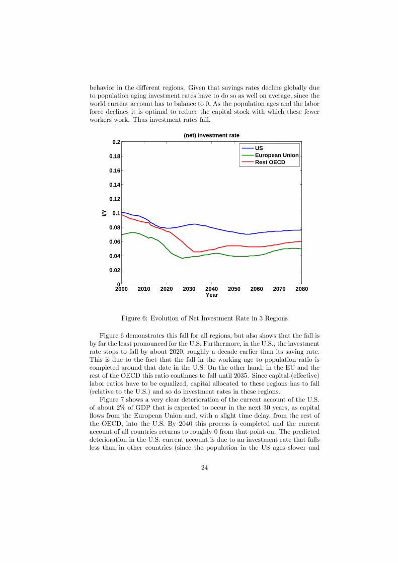
behavior in the different regions. Given that savings rates decline globally dueto population aging investment rates have to do so as well on average, since theworld current account has to balance to 0. As the population ages and the laborforce declines it is optimal to reduce the capital stock with which these fewerworkers work. Thus investment rates fall.

2000 2010 2020 2030 2040 2050 2060 2070 20800

0.02

0.04

0.06

0.08

0.1

0.12

0.14

0.16

0.18

0.2

Year

I/Y

(net) investment rate

USEuropean UnionRest OECD

Figure 6: Evolution of Net Investment Rate in 3 Regions

Figure 6 demonstrates this fall for all regions, but also shows that the fall isby far the least pronounced for the U.S. Furthermore, in the U.S., the investmentrate stops to fall by about 2020, roughly a decade earlier than its saving rate.This is due to the fact that the fall in the working age to population ratio iscompleted around that date in the U.S. On the other hand, in the EU and therest of the OECD this ratio continues to fall until 2035. Since capital-(effective)labor ratios have to be equalized, capital allocated to these regions has to fall(relative to the U.S.) and so do investment rates in these regions.Figure 7 shows a very clear deterioration of the current account of the U.S.

of about 2% of GDP that is expected to occur in the next 30 years, as capitalflows from the European Union and, with a slight time delay, from the rest ofthe OECD, into the U.S. By 2040 this process is completed and the currentaccount of all countries returns to roughly 0 from that point on. The predicteddeterioration in the U.S. current account is due to an investment rate that fallsless than in other countries (since the population in the US ages slower and

24

thus the labor force falls less) as well as a (temporary) sharp decline in theU.S. savings rate in the next 20 years due to the gradual retirement of the babyboomers (see again figures 5 and 6).

2000 2010 2020 2030 2040 2050 2060 2070 2080−0.03

−0.02

−0.01

0

0.01

0.02

0.03

Year

CA

/Y

current account / output ratio

USEuropean UnionRest OECD

Figure 7: Evolution of the Current Account in 3 Regions

Finally figure 8 shows the evolution of the net foreign asset position, relativeto GDP, in the three regions of our model. The European Union, as the oldestregion, has a positive net asset position and thus provides capital to both therest of the OECD and, increasingly, to the U.S.. As the U.S. current accountis strongly negative during the years 2020 and 2040, the U.S. net foreign assetposition reaches a trough of about −36% in about 2040. Thus the qualitativeresults from the quantitative model are in line with the predictions of the simplemodel, coupled with the level and dynamics of the working age to populationratio in the different regions documented in figure 2.

5.4 Distributional and Welfare Consequences of Demo-graphic Change

In the previous sections we have documented substantial changes in factor pricesinduced by the aging of the population, amounting to a decline of about 1percentage point in real returns to capital and an increase in gross wages of about

25

2000 2010 2020 2030 2040 2050 2060 2070 2080−1

−0.8

−0.6

−0.4

−0.2

0

0.2

0.4

0.6

0.8

1

Year

F/Y

foreign assets ratio

USEuropean UnionRest OECD

Figure 8: Evolution of the Net Foreign Asset Position in 3 Regions

4% in the next decades. In this section we want to quantify the distributionaland welfare effects emanating from these changes.

5.4.1 Evolution of Inequality

In figure 9 we display the evolution of income inequality over time in the threeregions. Income is composed of labor income (which later will include pensionincome) and capital income as well as transfers from accidental bequests.We observe a significant increase in income inequality between 2000 and

2080, of about 5 points in the Gini coefficient for the EU and the ROECDand 3.5 points in the U.S.. The reason for this increase is mainly a composi-tional effect. Retired households have significantly lower income on average thanhouseholds in working age. The demographic transition towards more retiredhouseholds therefore is bound to increase inequality, especially in those regionswhere the increase in the fraction of retired households among the population isvery pronounced. This explains the more modest increase in income inequalityin the U.S.. Note that consumption inequality follows income inequality trendsfairly closely in the three regions (and thus is not shown here), but increasesin consumption inequality are less pronounced. Also notice that the orderingof countries in the figure will be reversed once we add pension systems - then,

26

2000 2010 2020 2030 2040 2050 2060 2070 20800.4

0.42

0.44

0.46

0.48

0.5

0.52

0.54

0.56

0.58

Year

Gin

i co

effi

cien

t (i

nco

me)

Gini coefficient for income

USEuropean UnionRest OECD

Figure 9: Evolution of Income Inequality in 3 Regions

income will be least equally distributed in the U.S..The fact that it is not a rise in capital income inequality that drives the in-

crease in total income inequality becomes clear when plotting wealth inequalityover time. There is no discernible increase in the same period; evidently thesame is true for capital income inequality since capital income is proportionalto wealth.In contrast to income, wealth follows a hump-shaped pattern over the life

cycle (on average), with the elderly and the young being wealth-poor. Thus,in contrast to income inequality, the aging of the population does not lead toan increase in wealth inequality, since the demographic change increases thefraction of the elderly, but reduces the fraction of the young. Consequentlyincome and wealth inequality do not follow the same trend over time, nor is theranking in inequality across regions the same for income and wealth.We therefore conclude that the opposite general equilibrium effects on wages

and interest rates have little impact on the income and wealth distribution acrossgenerations.

27

2000 2010 2020 2030 2040 2050 2060 2070 20800.6

0.62

0.64

0.66

0.68

0.7

0.72

0.74

0.76

0.78

0.8

Year

Gin

i co

effi

cien

t (w

ealt

h)

Gini coefficient for wealth

USEuropean UnionRest OECD

Figure 10: Evolution of Wealth Inequality in 3 Regions

5.4.2 Welfare Consequences of the Demographic Transition

A household’s welfare is affected by two consequences of demographic change.First, her lifetime utility changes because her own survival probabilities increase;this is in part what triggers the aging of the population. Second, due to thedemographic transition she faces different factor prices and government transfersand taxes (from the social security system and from accidental bequests) thanwithout changes in the demographic structure. Specifically, households face apath of declining interest rates and increasing wages, relative to the situationwithout a demographic transition.We want to isolate the welfare consequences of the second effect. For this we

compare lifetime utility of agents born and already alive in 2005 under two differ-ent scenarios. For both scenarios we fix a household’s individual survival prob-abilities at their 2005 values; of course they fully retain their age-dependence.Then we solve each household’s problem under two different assumptions aboutfactor prices (and later taxes/transfers, once we have introduced social security).Let W (t, i, j, k, η, a) denote the lifetime utility of an agent at time t ≥ 2005 incountry i with individual characteristics (j, k, η, a) that faces the sequence ofequilibrium prices as documented in the previous section, but constant 2005survival probabilities, and let W 2005(t, i, j, k, η, a) denote the lifetime utility of

28

the same agent that faces prices and taxes/transfers that are held constant attheir 2005 value. Finally, denote by g(t, i, j, k, η, a) the percentage increase inconsumption that needs to be given to an agent (t, i, j, k, η, a) at each date andcontingency in her remaining lifetime (keeping labor supply allocations fixed)at fixed prices to make her as well off as under the situation with changingprices.9 Positive numbers of g(t, i, j, k, η, a) thus indicate that households obtainwelfare gains from the general equilibrium effects of the demographic changes,negative numbers mean welfare losses. Of particular interest are the numbersg(t = 56, i, j = 0, k, η, a = 0), that is, the welfare consequences for newbornagents in 2005 (t = 56) (remember that newborns start their life with zeroassets).Table IV documents these numbers for type 1 for the U.S., differentiated by

their productivity shock η. The results for type 2 are nearly identical.10

Table IV: Welfare Cons., USProductivity η1 Productivity η2

0.9% 0.6%

We make several observations. First, newborn agents experience welfaregains from changing factor prices and transfers induced by the demographictransition. Apart from changing preferences through higher longevity (an ef-fect we control for in our welfare calculations) the demographic transition sub-stantially increases the real wage over time, reduces the interest rate and firstincreases and then (after 2040) somewhat reduces transfers from accidental be-quests. The effect from changes in transfers is small, at least for newborns.The dominating effect for newborn agents is the substantial increase in wages,partially because these agents have not yet accumulated assets and thus do notsuffer from a loss of capital income on already accumulated financial wealth, incontrast to older households. Of course, a lower interest rate makes it harder forthese households to accumulate assets for retirement. Since borrowing is ruledout the decline in interest rates alone therefore has unambiguously negativeconsequences for welfare.Second, agents born with low productivity experience somewhat higher wel-

fare gains than agents that start their working life with high productivity. Lowproductivity agents expect higher productivity in the future, and thus bene-fit more strongly from the increasing wage profile induced by the demographic

9For the Cobb-Douglas utility specification for σ 6= 1 the number g(t, i, j, k, η, a) can easilybe computed as

g(t, i, j, k, η, a) =W (t, i, j, k, η, a)

W 2005(t, i, j, k, η, a)

1ωi(1−σ)

.

A similar expression holds for σ = 1.10The welfare consequences are very similar for other countries and type k2. In fact, in

the benchmark model the only difference across countries and types stems from accidentalbequests, which are redistributed in a lump-sum fashion and whose dynamics varies slightlyacross countries. Since these transfers are small in magnitude, however, so are the cross-country and cross-type differences in welfare.

29

transition than the currently highly productive, whose productivity is going tofall in expectation.

0 5 10 15−2

−1.8

−1.6

−1.4

−1.2

−1

−0.8

−0.6

−0.4

−0.2

0

Wel

fare

Ch

ang

eWelfare Consequences for age 60 in year 2005

Assets

low type, low shocklow type, high shockhigh type, low shockhigh type, high shock

Figure 11:

Given that the welfare impact of changing factor prices constitutes a trade-off between increasing wages and falling returns to capital one would expectthat those members of society for whom labor income constitutes a smaller partof (future) resources than capital income benefit less from the demographictransition. An advantage of our model with uninsurable idiosyncratic incomeshocks and thus endogenous intra-cohort wealth heterogeneity is that it allows usto document how the welfare consequences are distributed across the population,both across and within cohorts. Figure 11 plots the welfare gains for agents ofage 60 in 2005. These households have most of their working life behind them,thus are fairly unaffected by the wage changes, and simply experience lowerreturns on their accumulated savings. We see that agents in this cohort sufferwelfare losses which increase substantially by the amount of financial assetsthey have already accumulated. To give a sense of how many agents there areat different points in the asset distribution, the support of this distribution forthe 60 year old ranges roughly to a = 12 (about 19 times GDP per capita),with median asset levels around 4 (10) times GDP per capita for the low η - low(high) type agents and about 4.1 (10.8) times GDP per capita for the high η -low (high) type agents. Overall, a fraction of 38 percent of agents economically

30

alive in 2005 gain from the changing factor prices. These tend to be youngagents with little assets and currently low labor productivity.

5.5 The Role of Social Security (and its Reform)

So far, we completely abstracted from government policies. While it is notobvious a priori what the interaction of demographic changes and public policiesis in general, it is abundantly clear from policy debates that at least one largesocial program is strongly affected by it: social security.An idealized pay as you go public pension system can respond to an increase

in the share of pensioners in the population by (a combination of) at least threeways: cutting benefits, increasing social security contribution rates or increasingthe retirement age. While a likely response will include all elements, we nowpresent results for the model with a PAYGO social security system that respondsto population aging by either holding tax rates fixed (and thus cutting benefits),by holding replacement rates fixed (and thus raising taxes), or by increasing theretirement age.11 Because of the strong influence of a public pension system onprivate savings behavior, we expect that these different reform scenarios mayhave substantially different implications for the evolution of factor prices andthe size and direction of international capital flows as well as the distributionof welfare. This conjecture turns out to be correct. Note that for all exerciseswe re-calibrate production and preference parameters such that each economy(with the different social security systems) attains the same calibration targetsfor the 1950 to 2004 periodIn table V we show how the evolution of macroeconomic aggregates and

prices differs across the various scenarios for social security. Comparing theno-social security scenario to a world with social security in which payroll taxrates are held constant (and thus benefits decline), we observe that changesin factor prices are roughly the same between the two scenarios.12 One bigdifference, however, is the change in social security benefits required to copewith the demographic transition, which implies a decline in replacement ratesby about 8 percentage points in the scenario with social security. Column 4demonstrates that keeping pension benefits constant and adjusting taxes, onthe other hand, has dramatic consequences for the evolution of interest ratesand wages, relative to the benchmark scenario of fixing tax rates for socialsecurity. With fixed benefits the incentives to save for retirement are drasticallyreduced, relative to the benchmark. In addition, the substantial increase intax rates of 7 percentage points and the corresponding reduction in after taxwages makes it harder to save. Therefore, despite the decline in the fraction ofhouseholds in working age (and diminished incentives to work because of higherpayroll taxes) now the capital-labor ratio remains roughly unchanged, because

11 In our experiment we increase the mandatory retirement age by 5 years in 2005, and keepcontribution rates fixed. When needed, benefits are adjusted to retain budget balance of thesocial security system.12Remember that we recalibrate our model so that in all scenarios the pre-2005 equilibrium

features the same capital-output ratio.

31

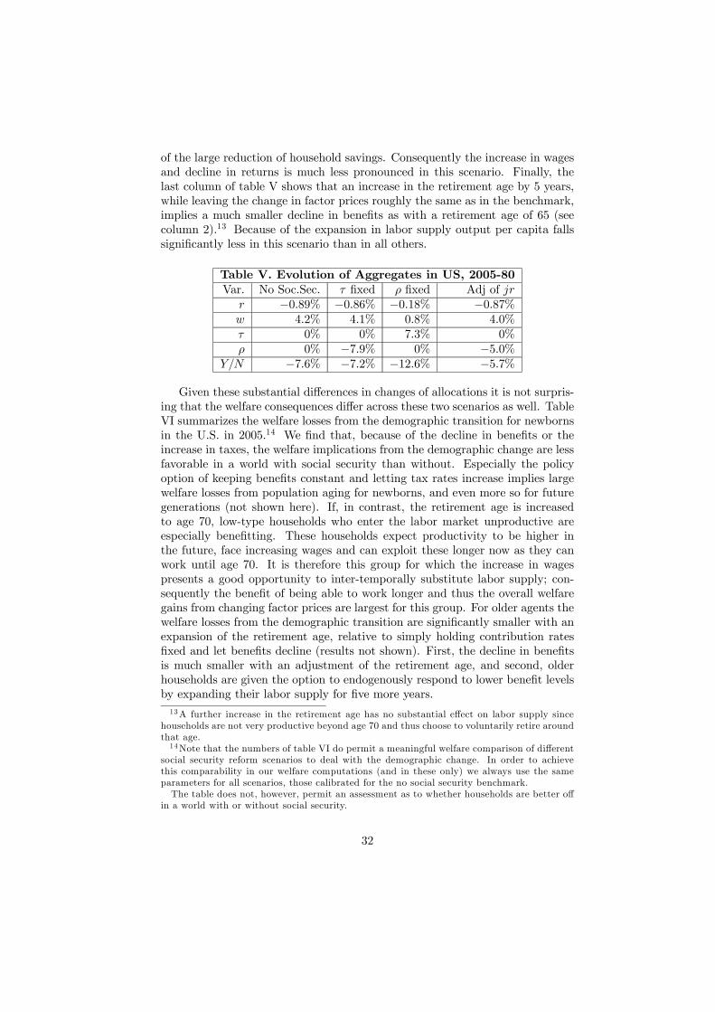
of the large reduction of household savings. Consequently the increase in wagesand decline in returns is much less pronounced in this scenario. Finally, thelast column of table V shows that an increase in the retirement age by 5 years,while leaving the change in factor prices roughly the same as in the benchmark,implies a much smaller decline in benefits as with a retirement age of 65 (seecolumn 2).13 Because of the expansion in labor supply output per capita fallssignificantly less in this scenario than in all others.

Table V. Evolution of Aggregates in US, 2005-80Var. No Soc.Sec. τ fixed ρ fixed Adj of jr

r −0.89% −0.86% −0.18% −0.87%w 4.2% 4.1% 0.8% 4.0%τ 0% 0% 7.3% 0%ρ 0% −7.9% 0% −5.0%

Y/N −7.6% −7.2% −12.6% −5.7%

Given these substantial differences in changes of allocations it is not surpris-ing that the welfare consequences differ across these two scenarios as well. TableVI summarizes the welfare losses from the demographic transition for newbornsin the U.S. in 2005.14 We find that, because of the decline in benefits or theincrease in taxes, the welfare implications from the demographic change are lessfavorable in a world with social security than without. Especially the policyoption of keeping benefits constant and letting tax rates increase implies largewelfare losses from population aging for newborns, and even more so for futuregenerations (not shown here). If, in contrast, the retirement age is increasedto age 70, low-type households who enter the labor market unproductive areespecially benefitting. These households expect productivity to be higher inthe future, face increasing wages and can exploit these longer now as they canwork until age 70. It is therefore this group for which the increase in wagespresents a good opportunity to inter-temporally substitute labor supply; con-sequently the benefit of being able to work longer and thus the overall welfaregains from changing factor prices are largest for this group. For older agents thewelfare losses from the demographic transition are significantly smaller with anexpansion of the retirement age, relative to simply holding contribution ratesfixed and let benefits decline (results not shown). First, the decline in benefitsis much smaller with an adjustment of the retirement age, and second, olderhouseholds are given the option to endogenously respond to lower benefit levelsby expanding their labor supply for five more years.13A further increase in the retirement age has no substantial effect on labor supply since

households are not very productive beyond age 70 and thus choose to voluntarily retire aroundthat age.14Note that the numbers of table VI do permit a meaningful welfare comparison of different

social security reform scenarios to deal with the demographic change. In order to achievethis comparability in our welfare computations (and in these only) we always use the sameparameters for all scenarios, those calibrated for the no social security benchmark.The table does not, however, permit an assessment as to whether households are better off

in a world with or without social security.

32

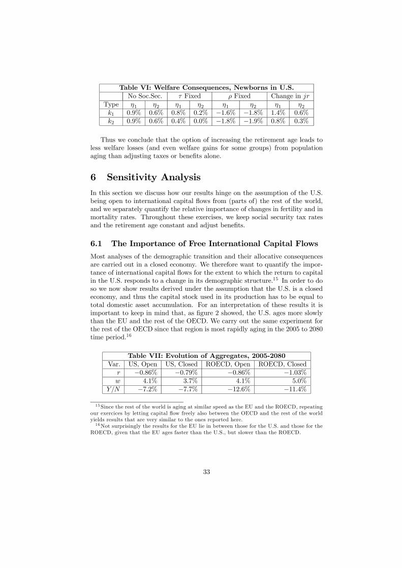
Table VI: Welfare Consequences, Newborns in U.S.No Soc.Sec. τ Fixed ρ Fixed Change in jr

Type η1 η2 η1 η2 η1 η2 η1 η2k1 0.9% 0.6% 0.8% 0.2% −1.6% −1.8% 1.4% 0.6%k2 0.9% 0.6% 0.4% 0.0% −1.8% −1.9% 0.8% 0.3%

Thus we conclude that the option of increasing the retirement age leads toless welfare losses (and even welfare gains for some groups) from populationaging than adjusting taxes or benefits alone.

6 Sensitivity AnalysisIn this section we discuss how our results hinge on the assumption of the U.S.being open to international capital flows from (parts of) the rest of the world,and we separately quantify the relative importance of changes in fertility and inmortality rates. Throughout these exercises, we keep social security tax ratesand the retirement age constant and adjust benefits.

6.1 The Importance of Free International Capital Flows

Most analyses of the demographic transition and their allocative consequencesare carried out in a closed economy. We therefore want to quantify the impor-tance of international capital flows for the extent to which the return to capitalin the U.S. responds to a change in its demographic structure.15 In order to doso we now show results derived under the assumption that the U.S. is a closedeconomy, and thus the capital stock used in its production has to be equal tototal domestic asset accumulation. For an interpretation of these results it isimportant to keep in mind that, as figure 2 showed, the U.S. ages more slowlythan the EU and the rest of the OECD. We carry out the same experiment forthe rest of the OECD since that region is most rapidly aging in the 2005 to 2080time period.16

Table VII: Evolution of Aggregates, 2005-2080Var. US, Open US, Closed ROECD, Open ROECD, Closed

r −0.86% −0.79% −0.86% −1.03%w 4.1% 3.7% 4.1% 5.0%

Y/N −7.2% −7.7% −12.6% −11.4%

15 Since the rest of the world is aging at similar speed as the EU and the ROECD, repeatingour exercices by letting capital flow freely also between the OECD and the rest of the worldyields results that are very similar to the ones reported here.16Not surprisingly the results for the EU lie in between those for the U.S. and those for the

ROECD, given that the EU ages faster than the U.S., but slower than the ROECD.

33

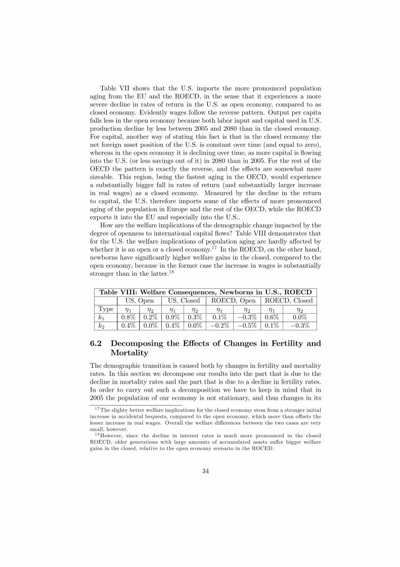
Table VII shows that the U.S. imports the more pronounced populationaging from the EU and the ROECD, in the sense that it experiences a moresevere decline in rates of return in the U.S. as open economy, compared to asclosed economy. Evidently wages follow the reverse pattern. Output per capitafalls less in the open economy because both labor input and capital used in U.S.production decline by less between 2005 and 2080 than in the closed economy.For capital, another way of stating this fact is that in the closed economy thenet foreign asset position of the U.S. is constant over time (and equal to zero),whereas in the open economy it is declining over time, as more capital is flowinginto the U.S. (or less savings out of it) in 2080 than in 2005. For the rest of theOECD the pattern is exactly the reverse, and the effects are somewhat moresizeable. This region, being the fastest aging in the OECD, would experiencea substantially bigger fall in rates of return (and substantially larger increasein real wages) as a closed economy. Measured by the decline in the returnto capital, the U.S. therefore imports some of the effects of more pronouncedaging of the population in Europe and the rest of the OECD, while the ROECDexports it into the EU and especially into the U.S..How are the welfare implications of the demographic change impacted by the

degree of openness to international capital flows? Table VIII demonstrates thatfor the U.S. the welfare implications of population aging are hardly affected bywhether it is an open or a closed economy.17 In the ROECD, on the other hand,newborns have significantly higher welfare gains in the closed, compared to theopen economy, because in the former case the increase in wages is substantiallystronger than in the latter.18

Table VIII: Welfare Consequences, Newborns in U.S., ROECDUS, Open US, Closed ROECD, Open ROECD, Closed

Type η1 η2 η1 η2 η1 η2 η1 η2k1 0.8% 0.2% 0.9% 0.3% 0.1% −0.3% 0.6% 0.0%k2 0.4% 0.0% 0.4% 0.0% −0.2% −0.5% 0.1% −0.3%

6.2 Decomposing the Effects of Changes in Fertility andMortality

The demographic transition is caused both by changes in fertility and mortalityrates. In this section we decompose our results into the part that is due to thedecline in mortality rates and the part that is due to a decline in fertility rates.In order to carry out such a decomposition we have to keep in mind that in2005 the population of our economy is not stationary, and thus changes in its

17The slighty better welfare implications for the closed economy stem from a stronger initialincrease in accidental bequests, compared to the open economy, which more than offsets thelesser increase in real wages. Overall the welfare differences between the two cases are verysmall, however.18However, since the decline in interest rates is much more pronounced in the closed

ROECD, older generations with large amounts of accumulated assets suffer bigger welfaregains in the closed, relative to the open economy scenario in the ROCED.

34

structure would occur even when mortality and fertility rates are held constantat their 2005 values.In order to account for these changes we first compute the consequences

from population aging assuming that mortality and fertility rates stay constantat their 2005 levels. By this, we isolate the impact of the population dynam-ics stemming from the nonstationary population structure in 2005. We thenin addition let either mortality or fertility rates change in accordance with UNpredictions and report the incremental change (over and above the pure pop-ulation dynamics) induced by the change in either mortality or fertility rates.Absent strong interaction effects the changes observed in the benchmark modelare then the sum of the pure population dynamics effect, the incremental ef-fect from changes in fertility rates and the incremental effect from changes inmortality rates.Table IX provides the outcome of this decomposition exercise and shows that

the main sources of changes in factor prices and other aggregates between 2005and 2080, at least in the U.S., come from changes in mortality rates (column 4of table IX), and from the fact that past fertility and mortality rates have led toa population structure that would imply an aging U.S. even absent any furtherchanges in fertility and mortality rates (column 2). In fact, since for the U.S.fertility rates (including migration rates) are predicted to increase slightly inthe near future, the effect from only changing fertility rates is to make the U.S.younger (see column 3). We also observe that indeed the consequences of thedemographic change can be almost perfectly be linearly dissected into to a purecomposition effect, a fertility rate effect and a mortality rate effect, as columns2-4 roughly sum to column 5, our benchmark results documented in section 5.Table IX also shows that future predicted changes in fertility and mortality

rates have substantially different impacts on interest rates r and savings ratessr. The strong decline in mortality rates alone makes people live longer andthus forces them to save more, but on the other hand shifts the populationtowards older cohorts (which tend to be dis-savers). On net, the savings rateincreases slightly. Since the fraction of the population in working age declinessubstantially (see the change in wapr in column 4), the capital-labor ratio in-creases, and with it wages; the rate of return falls as a consequence of decliningmortality rates. In contrast, while an increase in fertility also increases the sav-ings rate (since it shifts the population towards those that save, rather thandis-save), it also increases aggregate labor supply by enlarging the labor force.Thus the change in fertility rates alone reduces the capital-labor ratio and thusraises interest rates and reduces real wages.

35

Table IX: Evolution of Aggregates in the U.S., 2005-2080Var. Only Comp. Only ∆ Fertility Only ∆ Mortality Benchmarkwapr −8.4% 0.8% −4.2% −12.2%

sr −3.1% 0.7% 0.2% −2.5%r −0.45% 0.18% −0.66% −0.86%w 2.0% −0.8% 2.8% 4.1%ρ −6.3% 0.4% −1.8% −7.9%

Y/N −6.0% −0.3% −0.7% −7.2%

Overall, while predicted future changes in fertility rates are small and thusdo not affect aggregates between 2005 and 2080 substantially, the large declinein mortality rates predicted for the near future explains a substantial part ofthe increase in wages and the reduction of real interest rates, and thus, notsurprisingly, a substantial part of the welfare consequences from populationaging documented above.

7 ConclusionsIn all major industrialized countries the population is aging, bringing with ita potentially large impact on the returns to the production factors capital andlabor. This paper documents that the welfare consequences from the increase inwages and declines in rates of return can be substantial, in the order of up to 1%in lifetime consumption for newborns in 2005. These welfare gains for newbornshowever only come along if social security contribution rates are held constantat current levels. Households that have already accumulated assets, on theother hand, lose from the decline in rates of return. Increasing the mandatoryretirement age by five years is shown to substantially mitigate these losses andto significantly increase welfare gains of newborns.The welfare gains for newborns (and losses for older generations) we doc-

ument have to be added to (or traded off against) the potential welfare gainsfrom a longer (and healthier) life that is part of the source of the aging of thepopulation in industrialized countries. While quantifying these welfare gains isbeyond the scope of the current paper, our results indicate that overall livinglonger is likely to be a good thing for most households, at least if social securitytax rates are not increased to keep benefits constant at current levels.Another potentially beneficial side effect of a shrinking population (or a

less rapidly growing population) that we have abstracted from and that mayfurther enhance these welfare gains emanates from a reduction in the price ofhousing, assuming a supply that is at least somewhat inelastic. Since a seriousquantitative evaluation of this effect requires an appropriate model of housing(choice) and thus the need of adding a continuous state variable to our model,carrying out such an analysis is beyond the scope of current computationalfeasibility.Finally, one important channel of adjustment to a shrinking labor force that

we have abstracted from is endogenous human capital accumulation. Higher

36

returns to human capital in the form of higher wages may make it optimal foryoung (and possibly older) households to obtain a better education, increasingthe supply of effective labor. This effect may counteract some of the increasein the capital-labor ratio and hence mitigate the impact of population agingon factor prices. A quantitative exploration of this channel in a world with anaging population is left for future research.

References[1] Abel, A. (2003), “The Effects of a Baby Boom on Stock Prices and Capital

Accumulation in the Presence of Social Security,” Econometrica, 71,551-578.

[2] Altig, D., A. Auerbach, L. Kotlikoff, K. Smetters and J. Walliser (2001),“Simulating Fundamental Tax Reform in the U.S.,” American EconomicReview, 91, 574-595.

[3] Attanasio, O., S. Kitao and G. Violante (2006a), “Quantifying the Effectsof the Demographic Transition in Developing Economies,” Advances inMacroeconomics, 2, Article 2.

[4] Attanasio, O., S. Kitao and G. Violante (2006b), “Global DemographicTrends and Social Security Reform,” mimeo, New York University.

[5] Auerbach, A. and L. Kotlikoff (1987), Dynamic Fiscal Policy, CambridgeUniversity Press, Cambridge.

[6] Bloom, D. and J. Williamson (1998), “Demographic Transitions and Eco-nomic Miracles in Emerging Asia,” World Bank Economic Review,12(3), 419-455.

[7] Börsch-Supan, A, A. Ludwig and J. Winter (2006), “Aging, Pension Re-form, and Capital Flows: A Multi-Country Simulation Model,” forth-coming, Economica.

[8] Brooks, R. (2003), “Population Aging and Global Capital Flows in a Par-allel Universe,” IMF Staff Papers, 50, 200-221.

[9] Carroll, C. (2005), “The Methods of Endogenous Gridpoints for Solv-ing Dynamic Stochastic Optimization Problems,” CFS Working Paper2005/18.

[10] Conesa, J. and D. Krueger (1999), “Social Security Reform with Heteroge-neous Agents,” Review of Economic Dynamics, 2, 757-795.

[11] Conesa, J. and D. Krueger (2005), “On the Optimal Progressivity of theIncome Tax Code,” forthcoming, Journal of Monetary Economics.

[12] Deaton, A. (1991), “Saving and Liquidity Constraints,” Econometrica, 59,1221-1248.

[13] De Nardi, M., S. Imrohoroglu and T. Sargent (1999), “Projected U.S. de-mographics and Social Security,” Review of Economic Dynamics, 2, 575-615.

37

[14] Diamond, P. (1965), “National Debt in a Neoclassical Growth Model,”American Economic Review, 55, 1126-1150.

[15] Domeij, D. and M. Floden (2005), “Population Aging and InternationalCapital Flows,” forthcoming, International Economic Review.

[16] Fehr, H., S. Jokisch and L. Kotlikoff (2005), “The Developed World’s de-mographic Transition - The Role of Capital Flows, Immigration andPolicy,” in R. Brooks and A. Razin (eds.) Social Security Reform -Financial and Political Issues in International Perspective, CambridgeUniversity Press, Cambridge.

[17] Feroli, M. (2003), “Capital Flows Among the G-7 Nations: A DemographicPerspective,” mimeo, Federal Reserve Board

[18] Hansen, G. (1993), “The Cyclical and Secular Behavior of the Labor Input:Comparing Efficiency Units and Hours Worked,” Journal of AppliedEconometrics, 8, 71-80.

[19] Hendriksen, E. (2002), “A Demographic Explanation of U.S. and JapaneseCurrent Account Behavior,” mimeo, Carnegie Mellon University.

[20] Huang, H., S. Imrohoroglu and T. Sargent (1997), “Two Computations toFund Social Security,” Macroeconomic Dynamics, 1, 7-44.

[21] Imrohoroglu, A., S. Imrohoroglu and D. Joines (1995), “A Life Cycle Analy-sis of Social Security,” Economic Theory, 6, 83-114.

[22] Imrohoroglu, A., S. Imrohoroglu and D. Joines (1995), “Social Security inan Overlapping Generations Economy with Land,” Review of EconomicDynamics, 2, 638-665.

[23] Ludwig, A. (2005), “Moment Estimation in Auerbach-Kotlikoff Models:How Well Do They Match the Data?,” mimeo, MEA, University ofMannheim.

[24] Ludwig, A. (2006), “The Gauss-Seidel-Quasi-Newton Method: A HybridAlgorithm for Solving Dynamic Economic Models,” forthcoming, Jour-nal of Economic Dynamics and Control.

[25] Obstfeld, M. and K. Rogoff (1995), “The Intertemporal Approach to theCurrent Account,” in G. Grossman and K. Rogoff (eds.) Handbook ofInternational Economics, Vol. 3, Elsevier, Amsterdam.

[26] Storesletten, K., C. Telmer and A. Yaron (2004), “Consumption and RiskSharing over the Life Cycle,” Journal of Monetary Economics, 51, 609-633.

[27] United Nations (2002), “World Population Prospects: The 2002 Revision,”United Nations Population Division, United Nations, New York.

38

A Details of the Demographic ProjectionsFor each country i ∈ {1, . . . , I} we base our demographic data on the official de-mographic data and projections by the United Nations (United Nations, 2002).Starting from a given initial age-distribution of population, N0,j,i, in year 1950for actual age j ∈ {0, . . . , 96} demography in each year t is given recursively by

Nt+1,j+1,i = Nt,j,i(st,j,i +mt,j,i), mt,j,i = 0 for j > 20

Nt+1,0,i =50X

j=15

ft,j,iNt,j,i

where mt,j,i(ft,j,i) denotes time, age and country specific migration (fertility)rates. Our assumption, that migration rates are zero for ages above 20 allows usto treat newborns and immigrants in the economic model alike, compare Section3.1.The United Nations provide demographic data on Nt,j,i, st,j,i and ft,j,i on

an annual basis for the years 1950-2050, but for age-groups of five only. Weinterpolate the initial distribution of the population, N1950,j,i, and the dataon st,j,i and ft,j,i for all t ∈ {1950, . . . , 2050} between age-groups to get age-specific data. As for migration we use the UN data on aggregate migration,Mt,i, and assume that migration numbers are equally distributed across ages forj ∈ {0, . . . , 20}. These approximations result in a decent fit of our demographicmodel to the official aggregate UN figures.We further forecast demography beyond the UN forecasting horizon un-

til 2300. First, while holding fertility rates constant, we assume that life-expectancy continues to increase at constant rates until year 2100. We thenhold age-specific survival rates constant and assume that fertility rates adjustsuch that the number of newborns is constant in each successive year until2200. This adjustment procedure implies that stationary population numbersare reached in year 2200. To support the steady state in our economic model,we hold demography constant for an additional 100 years until 2300.

B Computational Details

B.1 Household Problem

The idea is to iterate on the Euler equation, using ideas developed in Carroll(2005). The dynamic programming problem of the household reads as

W (t, j, k, i, η, a) (19)

= maxc,a0,1−l

{u(c, 1− l) + βst,j,iXη0

π(η0|η)W (t+ 1, j + 1, k, i, η0, a0)}

s.t. c+ a0 =

((1− τ t,i)wt,iθkεjηl + (1 + rt)(a+ ht,i) for j < jr

bt,j,k,i + (1 + rt)(a+ ht,i) for j ≥ jr

a0, c ≥ 0 and l ∈ [0, 1]

39

where t indexes time, j indexes age, k indexes type, i indexes country, η denotesthe idiosyncratic income shock and a denotes asset holdings.Following Deaton (1991), we denote by x “cash-on-hand” as the amount of

resources available if l = 1,

x =

((1− τ t,i)wt,iθkεjη + (1 + rt)(a+ ht,i) for j < jr

bt,j,k,i + (1 + rt)(a+ ht,i) for j ≥ jr

Now, rewrite the Bellman equation as

V (t, j, k, , iη, x)

= maxc,1−l

{u(c, 1− l) + βst,j,i ·Xη0

π(η0|η)V (t+ 1, j + 1, k, i, η0, (1 + rt+1) (x− e) + y0)},

where

e =

(c+ wt,i(1− τ t,i)θkεjη(1− l) for j < jr

c for j ≥ jr

and

y0 =

(wt+1,i(1− τ t+1,i)θkεj+1η

0 + (1 + rt+1)ht+1,i for j < jr

bt+1,j+1,k,i + (1 + rt+1)ht+1,i for j ≥ jr

The resulting inter-temporal Euler equation for consumption reads as

uc ≥ βst,j,i(1 + rt+1)Xη0

π(η0|η)Vx0(t+ 1, j + 1, k, i, η0, x0)

= if a0 > 0 (20)

and the inter-temporal Euler equation for leisure as

u1−l ≥ βst,j,i(1 + rt+1)Xη0

π(η0|η)Vx0(t+ 1, j + 1, k, i, η0, x0)wt,i(1− τ t,i)θkεjη

= if l > 0 (21)

and the envelope condition reads as

Vx(t, j, k, i, η, x) = u0(c) (22)

We can therefore define the intra-temporal Euler equation between consump-tion and leisure as

u1−l ≥ ucwt,i(1− τ t,i)θkεjη

= if l > 0 and a0 > 0 (23)

40

from which, for the family of Cobb-Douglas utility functions, we can get anexplicit solution for leisure in terms of consumption and wages as

1− l = 1− l (c,wt,i(1− τ t,i)θkεjη)

if l > 0 and a0 > 0 (24)

Our algorithm operates on (20), (22) and (24).

1. Define a type-independent grid for savings

GA = {0, a2, . . . , ana}

2. Define a type-dependent grid on x for the last generation

GSJ,k = {x1,k, x1,k, . . . , xnx,k}

While GSJ,k is type dependent we drop the dependence on k from here on tosimplify notation. Choose xnx > ana as the maximum possible realizationof cash on hand and x1 = xmin > 0 as the minimum possible realizationof cash on hand. Furthermore let nx = na+ 1.

3. From economic theory it follows that

c(t, J, k, i, η, x) = x

l(t, J, k, i, η, x) = 0

a0(t, J, k, i, η, x) = 0

for all x ∈ GSJ,k. From (22)

V 0x0(t, J, k, i, η, x) = u0c(t, J, k, i, η, x)

Vx(t, J, k, i, η, x) = uc(t, J, k, i, η, x).

4. Now iterate on j, j = nj − 1, . . . , 1. Given that the function V 0x0(t+ 1, j +

1, k, i, η, x) is known from the previous step, do the following

(a) For all a0 ∈ GA, solve equation (20) for c using equation (24) fornumbers (c1, . . . , cna). Since

x0 /∈ GSj+1,k

in general, this involves interpolation of the function V . For reasonsof accuracy, we follow the suggestions of Carroll (2005) and interpo-late on an appropriate transform of V 0 which is approximately linear.

(b) Equipped with the consumption numbers, calculate leisure by solvingequation (24) for (l1, . . . , lna).. If l < 0 then go back to (a) andcalculate consumption for l = 0.

41

(c) Equipped with the consumption and leisure numbers, define the gridGSj,k by

x1 = xmin

xp+1 =

(ap + cp + (1− lp)wt,i(1− τ t,i)θkεjη for j < jr

ap + cp + bt,j,k,i for j < jr

for p = 1, . . . , na.

In general, x1 = xmin where xmin is the lowest possible realizationof cash on hand. If, however, xmin > x2 then replace x1 with anynumber smaller than x2.Calculate the consumption functions

c(t, j, k, i, η, x1) = x1

c(t, j, k, i, η, xp) = cp for p = 2, . . . , nx

l(t, j, k, i, η, xp) = lp for p = 1, . . . , nx

a(t, j, k, i, η, x1) = 0

a0(t, j, k, i, η, xp+1) = ap for p = 1, . . . , na

(d) Update for all x ∈ GSj,k

Vx(t, j, k, i, η, x)

= uc(c(t, j, k, i, η, x), 1− l(t, j, k, i, η, x))

V (t, j, k, i, η, x)

= u(c(t, j, k, i, η, x), 1− l(t, j, k, i, η, x)) + βst,j,iXη0

π(η0|η)V (t+ 1, j + 1, k, i, η0, x0)

The updating of the value function again involves interpolation.

B.2 The Aggregate Model

For a given r× 1 vector Ψ of structural model parameters, we first solve for an“artificial” initial steady state in period t = 0 which gives an initial distributionof assets. We thereby presume that households assume prices to remain constantfor all periods t ∈ {0, . . . , T} and are then surprised by the actual price changesinduced by the transitional dynamics. Next, we solve for the final steady stateof our model which is reached in period T and supported by our demographicprojections, see appendix A. For both steady states, we solve for the equilibriumof the aggregate model by iterating on the m×1 steady state price vector Pss =[p1, . . . , pm]

0. p1 is the world marginal product of capital, rt + δ, p2, . . . , pI+1are social security contribution (or replacement) rates of each country, τ t,i(ρt,i),and pI+2, . . . , p2I+1 are accidental bequests (as a ratio of wages) in each country,

42

ht,iwt,i

. Notice that all elements of Pss are defined such that they are constant inthe steady states.Solution for the steady states of the model involves the following steps:

1. In iteration q for guess P qss solve the household problem.

2. Next aggregate across all households in all countries to get the world-wide aggregate capital stock,

PiKt,i. Define by κt,i the capital stock per

efficiency unit in country i,

κt,i =Kt,i

Z1/(1−α)i AtLt,i

= κt ∀i,

which is constant across all countries by our assumption of perfect capitalmobility and the market market clearing condition for the world interestrate, rt + δ = ακα−1t . It follows thatX

i

Kt,i = κtXi

Z1/(1−α)i AtLt,i.

We use this condition to form an update of the world marginal product ofcapital, p1.

3. Aggregate across all households to get aggregate labor supply in each coun-try, Lt,i. Update social security contributions (or replacement rates) usingthe social security budget constraint, equation (16). Calculate bequestsin each country by equation (18).

4. Collect the updated variables in ˜Pss and notice that˜Pss = H(Pss), where

H is a vector-valued non-linear function.

5. Define the root-finding problem G(Pss) = Pss − H(Pss), where G is avector-valued non-linear function, and iterate on Pss until convergence.We use Broyden’s method to solve the problem and denote the final ap-proximate Jacobi matrix by Bss.

Next, we solve for the transitional dynamics by the following steps:

1. Use the steady state solutions to form a linear interpolation to get thestarting values for the m(T − 2) × 1 vector of equilibrium prices, P =[p01, . . . , p

0m]0, where pi, i = 1, . . . ,m are vectors of length (T − 2)× 1.

2. In iteration q for guess P q solve the household problem. We do so byiterating backwards in time for t = T − 1, . . . , 2 to get the decision rulesand forward for t = 2, . . . , T − 1 for aggregation.

3. Update variables as in the steady state solutions and denote by ˜P = H(P )the m(T − 2)× 1 vector of updated variables.

43

4. Define the root-finding problem asG(P ) = P−H(P ). Since T is large, thisproblem is substantially larger and we use the Gauss-Seidel-Quasi-Newtonalgorithm suggested in Ludwig (2006) to form and update guesses of anapproximate Jacobi matrix of the system ofm(T−2) non-linear equations.

B.3 Calibration of Structural Model Parameters

Calibration of structural model parameters is based on a procedure suggestedin Ludwig (2005). We split the r × 1 vector of structural model parameters,Ψ, as Ψ =

h(Ψe)0, (Ψf )0

i0. Ψf is a vector of predetermined (fixed) parameters,

whereas the e × 1 vector Ψe is estimated by minimum distance (unconditionalmatching of moments using e moment conditions). Denote by

ut(Ψe) = yt − f(Ψe) for t = 0, . . . , T0

the GMM error as the distance between data, yt, and model simulated (pre-dicted) values, f(Ψe).Under the assumption that the model is correctly specified, the restrictions

on the GMM error can be written as

E[ut(Ψe0)] = 0,

where Ψe0 denotes the vector of true values. Denote sample averages of ut as

gT0(Ψe) ≡ 1

T0 + 1

T0Xt=0

ut(Ψe). (25)

We estimate the elements of Ψe by setting these sample averages to zero (up tosome tolerance level).In our economic model, the vector Ψe is given by

Ψe = [g, δ, α, Zi, . . . , ZI , β, ωi, . . . , ωI ]0 .

We estimate the structural model parameters using data from various sourcesfor the period 1960, ..., 2004, hence T0 = 44. To identify the parameters ofthe production function, g, δ, α, we use NIPA data for the U.S. on GDP, fixedassets, depreciation, wages and labor supply. Since our economic model restrictsthe capital-output ratio to be equal across countries, we restrict Z1 = 1 andestimate Zi for i > 1 using data on labor productivity of country i relative to theU.S.. The remaining structural model parameters, β, ω1, ω2, ω3 are estimatedby simulation. We estimate β by setting to zero the average distance betweenthe simulated and the actual capital-output ratio and ω1, ω2, ω3 by setting tozero the average distance between simulated and actual average hours worked.The predetermined parameter of our model is the coefficient of relative riskaversion, σ, which we set to one. In addition, we impose the restriction that theparameters, α, δ, g, β, σ, are constant across countries.

44