NBER WORKING PAPER SERIES

MULTI-PERIOD CORPORATE FAILURE PREDICTIONWITH STOCHASTIC COVARIATES

Darrell DuffieKe Wang

Working Paper 10743http://www.nber.org/papers/w10743

NATIONAL BUREAU OF ECONOMIC RESEARCH1050 Massachusetts Avenue

Cambridge, MA 02138September 2004

We are grateful for helpful discussions with Takeshi Amemiya, Susan Athey, Richard Cantor, Roger Stein,Brad Effron, Robert Geske, Michael Gordy, Aprajit Mahajan, Staurt Turnbull, and Frank X. Zhang; forinsightful comments from seminar participants at Oxford University, Beijing University, SingaporeManagement University, Stanford University, SUNY Buffalo, Tsinghua University, The University ofCalifornia at Berkeley, The University of Tokyo, The University of Houston, and from participants in theMoody’s and NYU Inaugural Credit Risk Conference and The Bachelier World Congress; for excellentresearch assistance from Leandro Saita; and for a supporting grant from Moody’s. The views expressedherein are those of the author(s) and not necessarily those of the National Bureau of Economic Research.

©2004 by Darrell Duffie and Ke Wang. All rights reserved. Short sections of text, not to exceed twoparagraphs, may be quoted without explicit permission provided that full credit, including © notice, is givento the source.

Multi-Period Corporate Failure Prediction with Stochastic CovariatesDarrell Duffie and Ke WangNBER Working Paper No. 10743September 2004JEL No. C41, G33, E44

ABSTRACT

We provide maximum likelihood estimators of term structures of conditional probabilities of

bankruptcy over relatively long time horizons, incorporating the dynamics of firm-specific and

macroeconomic covariates. We find evidence in the U.S. industrial machinery and instruments

sector, based on over 28,000 firm-quarters of data spanning 1971 to 2001, of significant dependence

of the level and shape of the term structure of conditional future bankruptcy probabilities on a firm's

distance to default (a volatility-adjusted measure of leverage) and on U.S. personal income growth,

among other covariates.Variation in a firm's distance to default has a greater relative effect on the

term structure of future failure hazard rates than does a comparatively sized change in U.S. personal

income growth, especially at dates more than a year into the future.

Darrell DuffieGraduate School of BusinessStanford UniversityStanford, CA 94305-5015and NBERduffie@stanford.edu

Ke WangFaculty of EconomicsThe University of Tokyo7-3-1 Hongo, Bunkyo-kuTokyo, 113-0033Japankewang@e.u-tokyo.ac.jp

1 Introduction

We provide maximum likelihood estimators of term structures of conditionalcorporate bankruptcy probabilities. Our contribution over prior work is toexploit the dependence of failure intensities on stochastic covariates, as wellas the time-series dynamics of the covariates, in order to estimate the likeli-hood of failure over several future periods (quarters or years). We estimateour model for the U.S. industrial machinery and instrument sector, usingover 28,000 firm-quarters of data for the period 1971 to 2001. We find evi-dence of significant dependence of the level and shape of the term structureof conditional future failure probabilities on a firm’s distance to default (avolatility-adjusted measure of leverage) and on U.S. personal income growth,among other covariates. Variation in a firm’s distance to default has a greaterrelative effect on the term structure of future failure hazard rates than doesa comparatively sized change in the business-cycle covariate, U.S. personalincome growth, especially at dates more than one year into the future.

The estimated shape of the term structure of conditional failure prob-abilities reflects the time-series behavior of the covariates, especially lever-age targeting by firms and mean reversion in macroeconomic performance.The term structures of failure hazard rates are typically upward sloping atbusiness-cycle peaks, and downward sloping at business-cycle troughs, to adegree that depends on corporate leverage relative to its long-run target.

A firm’s failure intensity is assumed to depend on both firm-specific andmacroeconomic state variables. Stochastic evolution of the combined Markovstate vector Xt causes variation over time in the failure intensity λt = Λ(Xt).The firm exits for other reasons, such as merger, acquisition, or privatization,with an intensity αt = A(Xt). The total exit intensity is thus αt + λt.

We specify a doubly-stochastic formulation of the point process for failureand other forms of exit under which the conditional probability at time t ofcorporate survival (from failure or other exit) for s years is

p(Xt, s) = E

(

e−R

t+s

t(λ(u)+α(u)) du

∣

∣

∣

∣

Xt

)

, (1)

and under which the conditional probability of failure within s years is

q(Xt, s) = E

(∫ t+s

t

e−R

z

t(λ(u)+α(u)) duλ(z) dz

∣

∣

∣

∣

Xt

)

. (2)

1

This calculation of q(Xt, s), demonstrated in Section 2, reflects the fact that,in order to fail at time z, the firm must survive until time z, avoiding bothfailure and other forms of exit, which arrive at a total intensity of λ(u)+α(u).

While, as explained in Section 1.1, there is a significant prior literaturetreating the estimation of one-period-ahead bankruptcy probabilities, for ex-ample with logit models, we believe that this is the first empirical study ofthe conditional term structure of failure probabilities over multiple futuretime periods that incorporates the time dynamics of the covariates. The soleexception seems to be the practice of certain banks and dealers in structuredcredit products of treating the credit rating of a firm as though a Markovchain, with ratings transition probabilities estimated as long-term averageratings transition frequencies.1 It is by now well understood, however, thatthe current rating of a firm does not incorporate much of the influence of thebusiness cycle on failure rates (Nickell, Perraudin, and Varotto (2000), Kav-vathas (2001), Wilson (1997a), Wilson (1997b)), nor even the effect of priorratings history (Behar and Nagpal (1999), Lando and Skødeberg (2002)).There is, moreover, significant heterogeneity in the short-term failure prob-abilties of different firms of the same current rating (Kealhofer (2003)).

We anticipate several types of applications for our work, including (i) theanalysis by a bank of the credit quality of a borrower over various futurepotential borrowing periods, for purposes of loan approval and pricing, (ii)the determination by banks and bank regulators of the appropriate level ofcapital to be held by a bank, in light of the credit risk represented by itsloan portfolio, especially given the upcoming Basel II accord, under whichborrower default probabilities are to be introduced for the purpose of deter-mining the capital to be held as backing for a loan to a given borrower, (iii)the determination of credit ratings by rating agencies, and (iv) the ability toshed some light on the macroeconomic links between business-cycle variablesand the failure risks of corporations.

Absent a model that incorporates the dynamics of the underlying covari-ates, it seems difficult to extrapolate prior models of one-quarter-ahead orone-year-ahead default probabilities to longer time horizons. While one couldseperately estimate models of fixed-horizon failure probabilities for each ofvarious alternative time horizons, it is statistically more efficient to incor-porate joint consistency conditions for failure probabilities at various timehorizons within one model.

1See, for example, Duffie and Singleton (2003), Chapter 4.

2

The conditional survival and failure probabilities, p(Xt, s) and q(Xt, s)respectively, depend on:

• a parameter vector β determining the dependence of the failure andother-exit intensities, Λ(Xt) and A(Xt), respectively, on the covariatevector Xt, and

• a parameter vector γ determining the time-series behavior of the un-derlying state vector Xt of covariates.

The doubly-stochastic assumption, stated more precisely in Section 2, isthat, conditional on the paths of the underlying state variables determiningfailure and other-exit intensities for all firms, these exit times are the firstevent times of independent Poisson processes with the same (conditionallydeterministic) intensity paths.2 In particular, this means that, given the pathof the state-vector process, the merger and failure times of different firms areconditionally independent.

A major advantage of the doubly-stochastic formulation is that it al-lows decoupled maximum-likelihood estimations of β and γ, which can thenbe combined to obtain the maximum-likelihood estimators of the survivaland failure probabilities, p(Xt, s) and q(Xt, s), and other properties of themodel, such as probabilities of joint failure of more than one firm. We showthat, because of the doubly-stochastic assumption, the maximum likelihoodestimator of the intensity parameter vector β is the same as that of a con-ventional competing-risks duration model with time-varying covariates. Themaximum likelihood estimator of the time-series parameter vector γ woulddepend of course on the particular specification adopted for the time-seriesbehavior of the state process X. Our approach is quite flexible in that re-gard. For examples, we could allow the state process X to have GARCHvolatility behavior, to depend on hidden Markov chain “regimes,” or to havejump-diffusive behavior. For our specific empirical application to the U.S.machinery and instrument sector, we have adopted a simple Gaussian vectorauto-regressive specification for the firm-specific leverage variables and themacroeconomic growth variables, and we show that, in our setting, a con-ventional maximum-likelihood estimator for the associated parameter vectorγ can be used. A further advantage of this methodology is that it allows

2One must take care in interpreting this characterization when treating the “internalcovariates,” those that are firm-specific and therefore no longer available after exit, asexplained in Section 2.

3

straightforward maximum-likelihood estimation of the term structure of fail-ure probabilities, by simply substituting the maximum-likelihood estimatorsfor β and γ into (2). Asymptotic confidence intervals for the term structuresof failure probabilities can then be obtained by the usual “Delta method,”as explained in Appendix C.

The doubly-stochastic assumption is overly restrictive in settings for whichfailure or another form of exit by one firm could have an important directinfluence on the failure or other-exit intensity of another firm. This influencewould be anticipated to some degree if one firm plays a relatively large role inthe marketplace of another. Tests for this property developed in Das, Duffie,and Kapadia (2004) are not yet conclusive, with currently available data, asdiscussed in Section 3.1. Our empirical results should therefore be treatedwith caution.

In our study of the U.S. industrial machinery and instrument sector be-tween 1971 and 2001, we find that corporate failure probabilities dependsignificantly on both firm leverage and business-cycle covariates. We usea volatility-corrected measure of leverage, distance to default, that has be-come a standard default covariate in industry practice (Kealhofer 2003). Weillustrate the degree of dependence of long-horizon failure probabilities onthe time-series behavior of the covariates, principally through the effects ofmean reversion, long-run means, and volatilities of distances to default andof national income growth.

Our methods also lead to a calculation at time t of the conditional prob-ability P (T ∈ [t, u]∪q(Xu, s) > q |Xt) that the failure time T of a givenfirm is before some given future time u, or that the firm’s s-year failure prob-ability at time u will exceed a given level q. This and related calculationscould play a role in credit rating, risk management, and regulatory applica-tions. The estimated model can be further used to calculate probabilities ofjoint failure of groups of firms, or other properties related to failure corre-lation. In our doubly-stochastic model setting, failure correlation betweenfirms arises from correlation in their failure intensities due to (i) commondependence of these intensities on macro-variables and (ii) correlation acrossfirms of changes in leverage and other firm-specific covariates.

Our econometric methodology may be useful in other subject areas re-quiring estimators of multi-period survival probabilities under exit intensitiesthat depend on covariates with pronounced time-series dynamics. Examplesmight include the timing of real options such as technology switch, mort-gage prepayment, securities issuance, and labor mobility. We are unaware

4

of previously available econometric methodology for multi-period event pre-diction under stochastic covariates. That is, while there has been extensiveresearch on multi-period event prediction (for example, baseline-hazard du-ration models) including default,3 and while there is a separate literatureon event intensity estimation, we are not aware of prior work that estimatesmulti-period event probabilities with intensities that depend on stochastictime-varying covariates.

1.1 Related Literature

A standard structural model of bankruptcy timing assumes that a corpora-tion fails when its assets drop to a sufficiently low level relative to its liabili-ties. For example, the prototypical models of Black and Scholes (1973), Mer-ton (1974), Fisher, Heinkel, and Zechner (1989), and Leland (1994), take theasset process to be a geometric Brownian motion. In these models, a firm’sconditional failure probability is completely determined by its distance todefault, which is the number of standard deviations of annual asset growthby which the current asset level exceeds the firm’s liabilities. This failurecovariate, using market equity data and accounting data for liabilities, hasbeen adopted in industry practice by Moody’s KMV, a leading provider ofestimates of failure probabilties for essentially all publicly traded firms. (SeeCrosbie and Bohn (2002) and Kealhofer (2003).) Based on this theoreticalfoundation, it seems natural to include distance to default as a covariate.

In the context of a standard structural default model of this type, Duffieand Lando (2001) show that if the distance to default cannot be accuratelymeasured, then a filtering problem arises, and the failure intensity dependson the measured distance to default and also on other covariates that mayreveal additional information about the firm’s conditional failure probability.

More generally, a firm’s financial health may have multiple influencesover time. For example, firm-specific, sector-wide, and macroeconomic statevariables may all influence the evolution of corporate earnings and leverage.Given the usual benefits of parsimony, the preliminary model of long-horizonfailure probabilities estimated in this paper adopts two failure covariates,only, distance to default and U.S. personal income growth. (Other macroe-conomic performance measures could be used, as discussed in Section 3.2.)

3For multi-period default prediction in a setting with constant intensities, see for ex-ample Philosophov and Philiosophov (2002).

5

Given distance to default, the choice of a second covariate calls for a tradeoffbetween variables that are more directly tied to the firm’s marketplace (suchas sector performance measures), and variables that capture information thatis not largely explained by distance to default.

Prior empirical models of corporate failure probabilities, reviewed byJones (1987) and Hillegeist et al. (2003), have relied on many types of covari-ates, both fixed and time-varying. Prior work has not, however, attemptedto estimate failure probabilities over multiple time periods in a manner thatexploits the time-series behavior of the covariates.

The first generation of empirical corporate failure analysis originated withBeaver (1966), Beaver (1968a), Beaver (1968b), and Altman (1968), whoapplied multivariate discriminant analysis. Among the covariates in Altman’s“Z-score” is a measure of leverage, defined as the market value of equitydivided by the book value of total debt. Our distance to default covariate isessentially a volatility-corrected measure of leverage. In work independent ofours, Bharath and Shumway (2004) use a standard Cox proportional hazardmodel to confirm that distance to default is indeed a dominant covariate,while still finding some role for additional covariates, as do we.

A second generation of empirical work is based on qualitative-responsemodels, such as logit and probit. Among these, Ohlson (1980) used an “O-score” method in his year-ahead failure prediction model.

The latest generation of modeling is dominated by duration analysis.Early in this literature is the work of Lane, Looney, and Wansley (1986) onbank failure prediction, using time-independent covariates.4 These modelstypically apply a Cox proportional-hazard model. Lee and Urrutia (1996)used a duration model based on a Weibull distribution of failure time. Theycompare duration and logit models in forecasting insurer insolvency, findingthat, for their data, a duration model identifies more significant variablesthan does the logit model.

Duration models based on time-varying covariates include those of Mc-Donald and Van de Gucht (1999), in a model of the timing of high-yield bondfailures and call exercises.5 Related duration analysis by Shumway (2001),Kavvathas (2001), Chava and Jarrow (2002), and Hillegeist, Keating, Cram,and Lundstedt (2003) predict bankruptcy.6

4Whalen (1991) and Wheelock and Wilson (2000) also used Cox proportional-hazardmodels for bank failure analysis.

5Meyer (1990) used a similar approach in a study of unemployment duration.6Kavvathas (2001) also analyzes the transition of credit ratings.

6

Shumway (2001) uses a discrete duration model with time-dependent co-variates. Computationally, this is equivalent to a multi-period logit modelwith an adjusted-standard-error structure. In predicting one-year failure,Hillegeist, Keating, Cram, and Lundstedt (2003) also exploit a discrete du-ration model. By taking as a covariate the theoretical probability of failureimplied by the Black-Scholes-Merton’s model, based on distance to default,Hillegeist, Keating, Cram, and Lundstedt (2003) find, at least in this modelsetting, that distance to default does not entirely explain variation in failureprobabilities across firms. Accounting-based and macroeconomic variablesare also relevant. Our results confirm this conclusion for our data, and ex-tend the analysis to multiple period prediction. Further discussion of theselection of covariates for corporate failure prediction may be found in Sec-tion 3.2.

Moving from the empirical literature on corporate failure prediction to thestatistical methods available for this task, typical econometric treatments ofstochastic intensity models include those of Lancaster (1990) and Kalbfleischand Prentice (2002), which provide likelihood functions in settings similar toours.7 In their language, our macro-covariates are “external,” and our firm-specific covariates are “internal,” that is, cease to be generated once a firmhas failed. These sources do not treat large-sample properties, nor indeeddo large-sample properties appear to have been developed in a form suitablefor our application. For example, Berman and Frydman (1999) do provideasymptotic properties for maximum-likelihood estimators of stochastic inten-sity models, including a version of Cramer’s Theorem, but treat only casesin which the covariate vector Xt is fully external (with known transition dis-tribution), and in which event arrivals continue to occur, repeatedly, at thespecified parameter-dependent arrival intensity. This clearly does not treatour setting, for a firm typically disappears once it fails.8

7For other textbook treatments, see Andersen, Borgan, Gill, and Keiding (1992), Miller(1981), Cox and Isham (1980), Cox and Oakes (1984), Daley and Vere-Jones (1988), andTherneau and Grambsch (2000).

8For the same reason, the autoregressive conditional duration framework of Engle andRussell (1998) and Engle and Russell (2002) is not suitable for our setting, for the updatingof the conditional probability of an arrival in the next time period depends on whetheran arrival occured during the previous period, which again does not treat a firm thatdisappears once it fails.

7

2 Econometric Model

This section outlines our probabilistic model for corporate survival, and theestimators that we propose. The following section applies the estimator todata on the U.S. industrial machinery and instrument sector.

2.1 Conditional Survival and Failure Probabilities

Fixing a probability space (Ω,F , P ) and an information filtration Gt : t ≥ 0satisfying the usual conditions,9 let X = Xt : t ≥ 0 be a time-homogeneousMarkov process in R

d, for some integer d ≥ 1. The state vector Xt isa covariate for a given firm’s exit intensities, in the following sense. Let(M,N) be a doubly-stochastic non-explosive two-dimensional counting pro-cess driven by X, with intensities α = αt = A(Xt) : t ∈ [0,∞) for M andλ = λt = Λ(Xt) : t ≥ 0 for N , for some non-negative real-valued measur-able functions A( · ) and Λ( · ) on R

d. Among other implications, this meansthat, conditional on the path of X, the counting processes M and N areindependent Poisson processes with conditionally deterministic time-varyingintensities, α and λ, respectively. For details on these definitions, one mayrefer to Karr (1991) and Appendix I of Duffie (2001).

We suppose that a given firm exits (and ceases to be observable) at τ =inft : Mt + Nt > 0, which is the earlier of the first event time of N ,corresponding to failure, and the first event time of M , corresponding to exitfor some other reason. In our application to the U.S. industrial machineryand instrument sector, the portion of exits for reasons other than failure isfar too substantial to be ignored.

The main idea is that, so long as the firm has not exited for some reason,its failure intensity is Λ(Xt) and its intensity of exit for other reasons isA(Xt).

It is important to allow the state vector Xt to include firm-specific failurecovariates that cease to be observable when the firm exits at τ . For sim-plicity, we suppose that Xt = (Ut, Yt), where Ut is firm-specific and Yt ismacroeconomic. Thus, we consider conditioning by an observer whose in-formation is given by the smaller filtration Ft : t ≥ 0, where Ft is theσ-algebra generated by

(Us,Ms, Ns) : s ≤ min(t, τ) ∪ Ys : s ≤ t.9See Protter (1990) for technical definitions.

8

We now verify that the observer’s time-t conditional probabilities p(Xt, s)and q(Xt, s) of survival for s years, and of failure within s years, respectively,are as shown in (1) and (2). The firm’s failure time is the stopping timeT = inft : Nt > 0,Mt = 0.

Proposition 1. On the event τ > t of survival to t, the Ft-conditionalprobability of survival to time t+ s is

P (τ > t+ s | Ft) = p(Xt, s),

where p(Xt, s) is given by (1), and the Ft-conditional probability of failure byt+ s is

P (T < t+ s | Ft) = q(Xt, s),

where q(Xt, s) is given by (2).

Proof: We begin by conditioning instead on the larger information set Gt,and later show that this does not affect the calculation.

We first calculate that, on the event τ > t,

P (τ > t+ s | Gt) = p(Xt, s), (3)

and

P (T < t+ s | Gt) = q(Xt, s). (4)

The first calculation (3) is standard, using the fact that M +N is a doubly-stochastic counting process with intensity α+ λ. For the second calculation(4), we use the fact that, conditional on the path of X, the (improper)density, evaluated at any time z > t, of the failure time T , exploiting theX-conditional independence of M and N is, with the standard abuse ofnotation,

P (T ∈ dz |X) = P (infu : Nu 6= Nt ∈ dz,Mz = Mt |X)

= P (infu : Nu 6= Nt ∈ dz |X)P (Mz = Mt |X)

= e−R

z

tλ(u) duλ(z) dz e−

R

z

tα(u) du

= e−R

z

t(α(u)+λ(u)) duλ(z) dz.

From the doubly-stochastic property, conditioning also on Gt has no effecton this calculation, so

P (T ∈ [t, t+ s] | Gt, X) =

∫ t+s

t

e−R

z

t(α(u)+λ(u)) duλ(z) dz.

9

Now, taking the expectation of this conditional probability given Gt only,using the law of iterated expectations, leaves (4).

On the event τ > t, the conditioning information in Ft and Gt coincide.That is, every event contained by τ > t that is in Gt is also in Ft. Theresult follows.

One can calculate p(Xt, s) and q(Xt, s) explicitly in certain settings, forexample if the state vector X is affine and the exit intensities have affinedependence on X, as shown in various cases by Duffie, Pan, and Singleton(2000), Duffie, Filipovic, and Schachermayer (2003). In our eventual applica-tion, our specification of the dependence of the intensities on Xt is non-linear,which calls for numerical solutions of p(Xt, s) and q(Xt, s), as we shall seein Section 3. Fortunately, this numerical calculation is done after obtainingmaximum-likelihood estimates of the parameters of the model.

2.2 Maximum Likelihood Estimator

We turn to the problem of inference from data.For each of n firms, we let Ti = inft : Nit > 0,Mit = 0 denote the

failure time of firm i, and let Si = inft : Mit > 0, Nit = 0 denote thecensoring time for firm i due to other forms of exit. We let Uit be the firm-specific vector of variables that are observable for firm i until its exit timeτi = min(Si, Ti), and let Yt denote the vector of environmental variables(such as business-cycle variables) that are observable at all times. We letXit = (Uit, Yt), and assume, for each i, that Xi = Xit : t ≥ 0 is a Markovprocess.(This means that, given Yt, the transition probabilities of Uit do notdepend on Ujt for j 6= i, a simplifying assumption.) Because, in our currentimplementation of the model, we observe these covariates Xit only quarterly,we take Xit = Xi,k(t) = Zi,k(t), where k(t) denotes the last (integer) discretetime period before t, and where Zi is the time-homogeneous discrete-timeMarkov process of covariates for firm i. This means that Xi is constantbetween periodic observations, a form of time-inhomogeneity that involvesonly a slight extension of our basic theory of Section 2.1. We continue tomeasure time continuously, however, because we wish to allow the use ofinformation associated with the intra-period timing of exits.

Extending our notation from Section 2.1, for all i, we let Λ(Xit, β) andA(Xit, β) denote the failure and other-exit intensities of firm i, where β is aparameter vector, common to all firms, to be estimated. This homogeneityacross firms allows us to exploit both time-series and cross-sectional data,

10

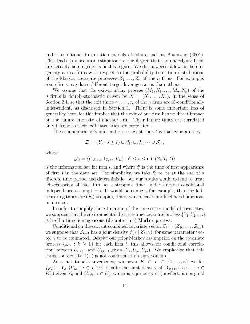
and is traditional in duration models of failure such as Shumway (2001).This leads to inaccurate estimators to the degree that the underlying firmsare actually heterogeneous in this regard. We do, however, allow for hetero-geneity across firms with respect to the probability transition distributionsof the Markov covariate processes Z1, . . . , Zn of the n firms. For example,some firms may have different target leverage ratios than others.

We assume that the exit-counting process (M1, N1, . . . ,Mn, Nn) of then firms is doubly-stochastic driven by X = (X1, . . . , Xn), in the sense ofSection 2.1, so that the exit times τ1, . . . , τn of the n firms areX-conditionallyindependent, as discussed in Section 1. There is some important loss ofgenerality here, for this implies that the exit of one firm has no direct impacton the failure intensity of another firm. Their failure times are correlatedonly insofar as their exit intensities are correlated.

The econometrician’s information set Ft at time t is that generated by

It = Ys : s ≤ t ∪ J1t ∪ J2t · · · ∪ Jnt,

whereJit = (1Si<s, 1Ti<s, Uis) : t0i ≤ s ≤ min(Si, Ti, t)

is the information set for firm i, and where t0i is the time of first appearanceof firm i in the data set. For simplicity, we take t0i to be at the end of adiscrete time period and deterministic, but our results would extend to treatleft-censoring of each firm at a stopping time, under suitable conditionalindependence assumptions. It would be enough, for example, that the left-censoring times are (Ft)-stopping times, which leaves our likelihood functionsunaffected.

In order to simplify the estimation of the time-series model of covariates,we suppose that the environmental discrete-time covariate process Y1, Y2, . . .is itself a time-homogeneous (discrete-time) Markov process.

Conditional on the current combined covariate vector Zk = (Z1k, . . . , Znk),we suppose that Zk+1 has a joint density f( · |Zk; γ), for some parameter vec-tor γ to be estimated. Despite our prior Markov assumption on the covariateprocess Zik : k ≥ 1 for each firm i, this allows for conditional correla-tion between Ui,k+1 and Uj,k+1 given (Yk, Uik, Ujk). We emphasize that thistransition density f( · ) is not conditioned on survivorship.

As a notational convenience, whenever K ⊂ L ⊂ 1, . . . , n we letfKL( · | Yk, Uik : i ∈ L; γ) denote the joint density of (Yk+1, Ui,k+1 : i ∈K) given Yk and Uik : i ∈ L, which is a property of (in effect, a marginal

11

of) f( · |Zk; γ). In our eventual application, we will further assume thatf( · | z; γ) is a joint-normal density, which makes the marginal density func-tion fKL( · | y, ui : i ∈ L) an easily-calculated joint normal.

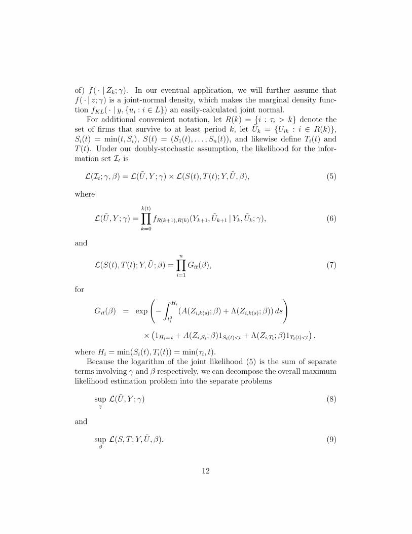
For additional convenient notation, let R(k) = i : τi > k denote theset of firms that survive to at least period k, let Uk = Uik : i ∈ R(k),Si(t) = min(t, Si), S(t) = (S1(t), . . . , Sn(t)), and likewise define Ti(t) andT (t). Under our doubly-stochastic assumption, the likelihood for the infor-mation set It is

L(It; γ, β) = L(U , Y ; γ) × L(S(t), T (t);Y, U, β), (5)

where

L(U , Y ; γ) =

k(t)∏

k=0

fR(k+1),R(k)(Yk+1, Uk+1 | Yk, Uk; γ), (6)

and

L(S(t), T (t);Y, U ; β) =n∏

i=1

Git(β), (7)

for

Git(β) = exp

(

−∫ Hi

t0i

(A(Zi,k(s); β) + Λ(Zi,k(s); β)) ds

)

×(

1Hi= t + A(Zi,Si; β)1Si(t)<t + Λ(Zi,Ti

; β)1Ti(t)<t

)

,

where Hi = min(Si(t), Ti(t)) = min(τi, t).Because the logarithm of the joint likelihood (5) is the sum of separate

terms involving γ and β respectively, we can decompose the overall maximumlikelihood estimation problem into the separate problems

supγ

L(U , Y ; γ) (8)

and

supβ

L(S, T ;Y, U, β). (9)

12

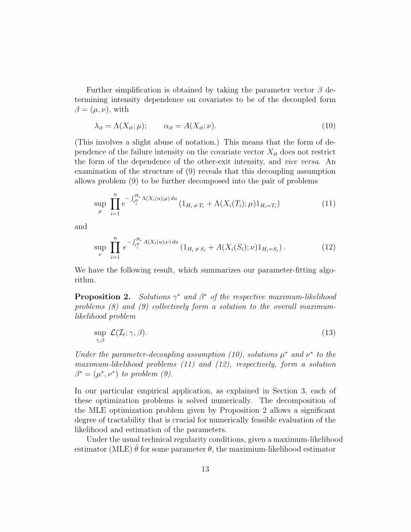
Further simplification is obtained by taking the parameter vector β de-termining intensity dependence on covariates to be of the decoupled formβ = (µ, ν), with

λit = Λ(Xit;µ); αit = A(Xit; ν). (10)

(This involves a slight abuse of notation.) This means that the form of de-pendence of the failure intensity on the covariate vector Xit does not restrictthe form of the dependence of the other-exit intensity, and vice versa. Anexamination of the structure of (9) reveals that this decoupling assumptionallows problem (9) to be further decomposed into the pair of problems

supµ

n∏

i=1

e−

R Hi

t0i

Λ(Xi(u);µ) du(1Hi 6=Ti

+ Λ(Xi(Ti);µ)1Hi=Ti) (11)

and

supν

n∏

i=1

e−

R Hi

t0i

A(Xi(u);ν) du(1Hi 6=Si

+ A(Xi(Si); ν)1Hi=Si) . (12)

We have the following result, which summarizes our parameter-fitting algo-rithm.

Proposition 2. Solutions γ∗ and β∗ of the respective maximum-likelihoodproblems (8) and (9) collectively form a solution to the overall maximum-likelihood problem

supγ,β

L(It; γ, β). (13)

Under the parameter-decoupling assumption (10), solutions µ∗ and ν∗ to themaximum-likelihood problems (11) and (12), respectively, form a solutionβ∗ = (µ∗, ν∗) to problem (9).

In our particular empirical application, as explained in Section 3, each ofthese optimization problems is solved numerically. The decomposition ofthe MLE optimization problem given by Proposition 2 allows a significantdegree of tractability that is crucial for numerically feasible evaluation of thelikelihood and estimation of the parameters.

Under the usual technical regularity conditions, given a maximum-likelihoodestimator (MLE) θ for some parameter θ, the maximium-likelihood estimator

13

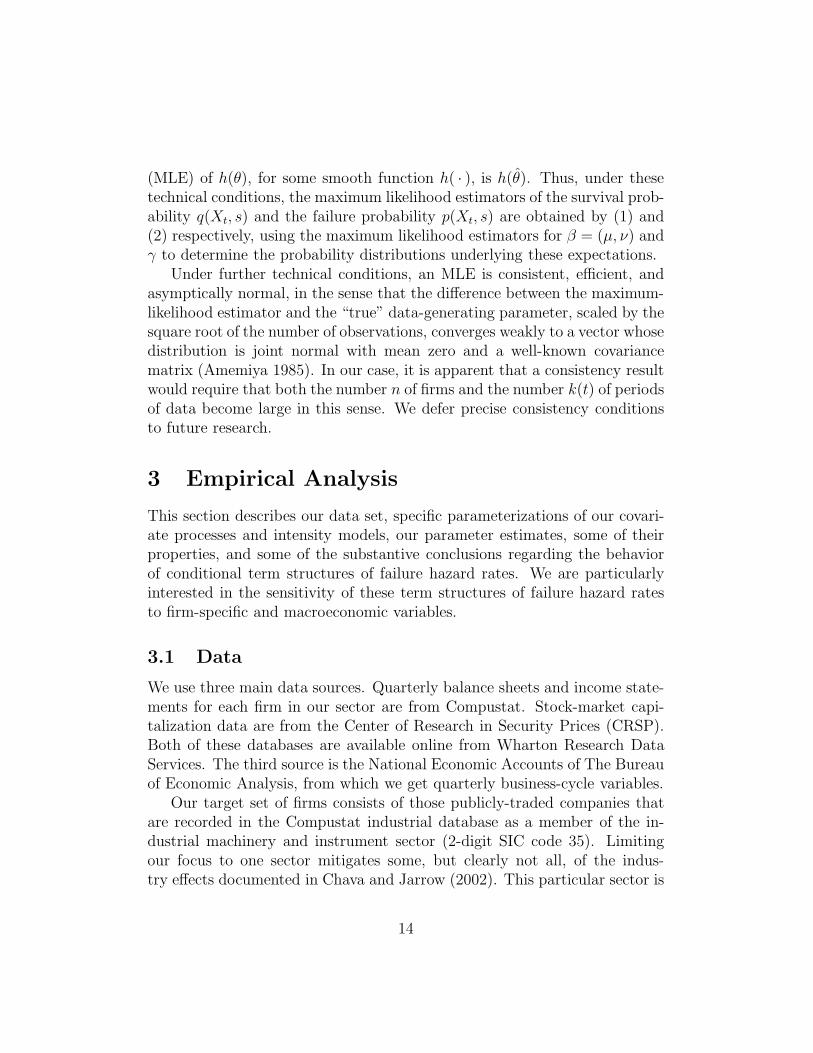
(MLE) of h(θ), for some smooth function h( · ), is h(θ). Thus, under thesetechnical conditions, the maximum likelihood estimators of the survival prob-ability q(Xt, s) and the failure probability p(Xt, s) are obtained by (1) and(2) respectively, using the maximum likelihood estimators for β = (µ, ν) andγ to determine the probability distributions underlying these expectations.

Under further technical conditions, an MLE is consistent, efficient, andasymptically normal, in the sense that the difference between the maximum-likelihood estimator and the “true” data-generating parameter, scaled by thesquare root of the number of observations, converges weakly to a vector whosedistribution is joint normal with mean zero and a well-known covariancematrix (Amemiya 1985). In our case, it is apparent that a consistency resultwould require that both the number n of firms and the number k(t) of periodsof data become large in this sense. We defer precise consistency conditionsto future research.

3 Empirical Analysis

This section describes our data set, specific parameterizations of our covari-ate processes and intensity models, our parameter estimates, some of theirproperties, and some of the substantive conclusions regarding the behaviorof conditional term structures of failure hazard rates. We are particularlyinterested in the sensitivity of these term structures of failure hazard ratesto firm-specific and macroeconomic variables.

3.1 Data

We use three main data sources. Quarterly balance sheets and income state-ments for each firm in our sector are from Compustat. Stock-market capi-talization data are from the Center of Research in Security Prices (CRSP).Both of these databases are available online from Wharton Research DataServices. The third source is the National Economic Accounts of The Bureauof Economic Analysis, from which we get quarterly business-cycle variables.

Our target set of firms consists of those publicly-traded companies thatare recorded in the Compustat industrial database as a member of the in-dustrial machinery and instrument sector (2-digit SIC code 35). Limitingour focus to one sector mitigates some, but clearly not all, of the indus-try effects documented in Chava and Jarrow (2002). This particular sector is

14

chosen mainly for the fact that among all sectors, it has the largest number ofbankruptcies recorded in the Compustat database during our sample period,1971 to 2001. Also, failures in this sector are not concentrated within a shorttime period, as is the case, for examples, in the banking and oil-and-gas sec-tors. A concentration of bankuptcies within a short time period would limitour ability to identify dependence of failure intensities on macroeconomicvariables.

Specifically, we include all firms of this sector for which the data necessaryto construct our covariates are available from Compustat and CRSP, withexceptions to be noted. In all, 870 such firms existed during our sampleperiod, of which 332 remain “active” as public firms, as of the end of oursample period, the end of 2001.

Of the remaining 538 firms, 70 failed, filing for bankruptcy under Chapter11 or Chapter 7 of the U.S. Bankruptcy Code. Coverage by Compustat ofthe remaining 468 firms was discontinued for other reasons, such as merger,acquisition, leveraged buyout, privatization, or ceasing to provide data.10

Exits are recorded by month in the Compustat annual file (item AFTNT33and item AFTNT34), and are assumed for purposes of our estimation tooccur at the end of the relevant month. Approximately 80% of the non-failure exits in our sample were due to merger and acquisition activities.

Among our sample of 870 firms, 50 firms existed before the January, 1971beginning of our sample period. As explained earlier, start dates are non-informative in our model. That is, with our probabilistic specification ofexit times, “left-censoring” does not call for an adjustment to the likelihoodfunction. In practice, however, there is likely to be some influence on failureintensities, given our other covariates, on survival time. One might estimatethis effect with a baseline hazard rate, which would call for a left-censorshipadjustment for the firms that existed before our sample period. There mayalso be calendar-time effects that we do not capture, for example due tochanges over time in the costs of raising new capital, as suggested by Famaand French (2004).

Our sample period begins at the first quarter of 1971, and ends11 at thefourth quarter of 2001. Although CRSP stock-price data are available from1925, and Compustat quarterly coverage of public firms begins in 1962, only

10The alternative forms of exit can be determined from Compustat item AFTNT35.11We include Compustat and CRSP variables from the fourth quarter of 1970 in order

to estimate the failure intensity during the first quarter of 1971. Likewise, lagged-quartervariables are used to fit the covariate time-series.

15

since 1972 has Compustat reported quarterly data on short-term liabilities,a relatively important determinant of our distance-to-default covariate.12 Inany case, of the 1, 283 failures in all industries recorded in Compustat, only9 are reported to have occured before 1971. Our decision to include onlypost-1971 data was also followed by Shumway (2001) and Vassalou and Xing(2003).

The doubly-stochastic assumption is overly restrictive in the presence ofstrong contagion effects, by which failure by one firm leads directly to asignificant increase in the likelihood of failure of other firms. This wouldbe the case, for example, if failure by a leading firm in an industry causesa significant weakening of other firms in the industry, above and beyondthe default correlation induced by common and correlated covariates, whichwe have already incorporated within our formulation. In the U.S. machineryand instruments sector during our study period, there were normally at mostthree to five corporate failures in a year, and we have no evidence suggest-ing significant direct failure contagion. Das, Duffie, and Kapadia (2004) testfor the doubly-stochastic property among all U.S. industries. While theyreject the joint hypothesis of correctly measured default probabilities andthe doubly-stochastic property, they provide some evidence that the defaultprobability data that they obtained from Moodys, based on only firm-specificcovariates, may have been responsible for this rejection, given the missedcorrelating effects of macroeconomic variables. Moreover, they test for, andfind no evidence of, clustering of defaults in excess of that suggested by thedoubly-stochastic property. In summary, while the doubly-stochastic prop-erty is without doubt restrictive and ignores some contagion effects that arelikely to be present, there is as yet no empirical evidence suggesting that itleads to significant distortions in default probability estimates. For our pur-pose of consistent and efficient multi-period default probability estimation,moreover, the doubly-stochastic property provides a framework that wouldnot be easily relaxed without significant loss of tractability.13

12The quality of pre-1971 Compustat data seems somewhat unreliable. For example,pre-1971 liability data for many companies are missing.

13With the large number of mergers and other exits in our data, one must also considerthe relevance of the doubly-stochastic assumption for merger and acquisition timing. Weleave this question for future consideration.

16

3.2 Covariates

We have examined the dependence of estimated failure and other-exit in-tensities on several types of firm-specific, sector-wide, and macroeconomicvariables. These include:

1. Distance to default, which, roughly speaking, is the number of standarddeviations of quarterly asset growth by which current assets exceed astandard measure of current liabilities. As explained in Section 1.1, thiscovariate has theoretical underpinnings in the Black-Scholes-Mertonstructural model of default probabilities. Our method of constructionof this covariate, based on market equity data and Compustat bookliability data, is along the lines of that used by Vassalou and Xing(2003), Crosbie and Bohn (2002), and Hillegeist, Keating, Cram, andLundstedt (2003). Details are given in Appendix A.

2. Personal income growth. As a measure of macroeconomic performance,we use U.S. personal income growth. Data on quarterly national per-sonal income (seasonally adjusted) is obtained from the Bureau of Eco-nomic Analysis’ National Economic Accounts database. Personal in-come growth is measured in terms of quarterly percentage changes. Ourselection of personal income growth as a representative macroeconomiccovariate is pragmatic; we found it to be more contemporaraneouslyand significantly correlated with failure rates than GDP growth rates.While one-quarter-lagged GDP growth rate has a significant and neg-ative role as a failure covariate if used as the sole macroeconomic co-variate, it has no significant role if used together with personal incomegrowth. Prior studies find correlation between macroeconomic condi-tions and failure, using a variety of macroeconomic variables. (SeeAllen and Saunders (2002) for a survey.) For example, McDonald andVan de Gucht (1999) used quarterly industrial production growth inthe U.S. as a covariate for high-yield bond failure. Hillegeist, Keat-ing, Cram, and Lundstedt (2003) exploit the national rate of corporatebankruptcies, in a baseline-hazard-rate model of default. Fons (1991),Blume and Keim (1991), and Jonsson and Fridson (1996) documentthat aggregate failure rates tend to be high in the downturn of businesscycles. Pesaran, Schuermann, Treutler, and Weiner (2003) use a com-prehensive set of country-specific macro variables to estimate the effectof macroeconomic shocks in one region on the credit risk of a global

17

loan portfolio. Keenan, Sobehart, and Hamilton (1999) and Helwegeand Kleiman (1997) model the forecasting of aggregate year-ahead U.S.default rates on corporate bonds, using, among other covariates, creditrating, age of bond, and various macroeconomic variables, includingindustrial production, interest rates, trailing default rates, aggregatecorporate earnings, and indicators for recession.

3. Sector earnings performance, measured as the sector average acrossfirms of the ratios of earnings to assets. When used as the only environ-mental covariate, sector earnings performance is indeed a statisticallysignificant covariate for failure intensity (although not for other-exitintensity). When included as an additional covariate together with dis-tance to default and personal income growth, however, sector earningsperformance does not appear to play a significant role.

4. Firm earnings performance, defined as the ratio of net income (Com-pustat item 69) to total assets (item 44). In contrast to distance to de-fault, this earnings covariate comes solely from accounting data. Sincethere is a lag in recording a firm’s accounting data, we lag earnings byone period in order to ensure that it is observable at the beginning ofthe quarter. (Because of this, firms enter our study only at the secondquarter after their first appearance in our database.) When there areoccassionally missing data for net income, we substitute values from themost immediately available past quarters. Earnings is complementaryto distance to default, and a traditional predictor for bankruptcy sinceAltman (1968). When not appearing together with distance to default,earnings is a significant failure covariate in both logit and durationmodels, as shown by Shumway (2001).14 Our definition of earnings isthat used by Zmijewski (1984), and close to the profitability covariatesdefined by Altman (1993), the ratio of retained earnings to total assets,and the ratio of earnings before interest and taxes to total assets.

5. Firm Size. We measure firm size as the logarithm of a firm’s bookvalue of total assets (Compustat item 44). Firm size may control forunobserved heterogeneity across firms, since big firms and small firmsmay have different market power, management strategies, or borrowing

14Another robustly significant factor according to Shumway’s paper is leverage ratio,but that has been incorporated in distance to default

18

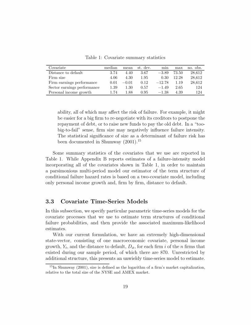
Table 1: Covariate summary statistics

Covariate median mean st. dev. min max no. obs.Distance to default 3.74 4.40 3.67 −3.89 73.50 28,612Firm size 4.06 4.30 1.95 0.30 12.28 28,612Firm earnings performance 0.01 −0.01 0.12 −12.78 1.19 28,612Sector earnings performance 1.39 1.30 0.57 −1.49 2.65 124Personal income growth 1.74 1.88 0.95 −1.38 4.39 124

ability, all of which may affect the risk of failure. For example, it mightbe easier for a big firm to re-negotiate with its creditors to postpone therepayment of debt, or to raise new funds to pay the old debt. In a “too-big-to-fail” sense, firm size may negatively influence failure intensity.The statistical significance of size as a determinant of failure risk hasbeen documented in Shumway (2001).15

Some summary statistics of the covariates that we use are reported inTable 1. While Appendix B reports estimates of a failure-intensity modelincorporating all of the covariates shown in Table 1, in order to maintaina parsimonious multi-period model our estimator of the term structure ofconditional failure hazard rates is based on a two-covariate model, includingonly personal income growth and, firm by firm, distance to default.

3.3 Covariate Time-Series Models

In this subsection, we specify particular parametric time-series models for thecovariate processes that we use to estimate term structures of conditionalfailure probabilities, and then provide the associated maximum-likelihoodestimates.

With our current formulation, we have an extremely high-dimensionalstate-vector, consisting of one macroeconomic covariate, personal incomegrowth, Yt, and the distance to default, Dit, for each firm i of the n firms thatexisted during our sample period, of which there are 870. Unrestricted byadditional structure, this presents an unwieldy time-series model to estimate.

15In Shumway (2001), size is defined as the logarithm of a firm’s market capitalization,relative to the total size of the NYSE and AMEX market.

19

After preliminary examination of various feasibly estimated alternatives, wehave opted for a simple specification in which each of Yt, D1t, . . . , Dnt is a uni-variate first-order auto-regressive Gaussian process, allowing for correlationamong their innovations.

Specifically, personal income growth in quarter k, Yk, is assumed to satisfy

Yk+1 − Yk = κY (θY − Yk) + σY εk+1, (14)

where ε1, ε2, . . . is an independent sequence of standard normal variables, andφ = (θY , κY , σY ) is a parameter vector to be estimated. Here, θY is the long-run mean, κY is the mean-reversion rate, and σY is the standard deviationof the innovations.

Similarly, for each firm i, for the quarters in which this firm appears inour sample,

Di,k+1 −Dik = κD(θDi −Dik) + vwi,k+1, (15)

where wik : k ≥ 1 is an independent sequence of standard normals, κD is amean-reversion parameter common to all firms, v is an innovations standard-deviation parameter common to all firms, and θDi is a long-run mean16 pa-rameter that is specific to firm i. The parameters v and κD characterizethe degree of volatility and mean reversion in this leverage-related variable.Volatility arises from uncertainty in earnings performance and in the revalu-ation of assets and liabilities. Mean-reversion arises from leverage targeting,by which corporations commonly pay out dividends and other forms of distri-butions when they achieve a sufficiently low degree of leverage, and converselyattempt to raise capital and retain earnings to a higher degree when theirleverage introduces financial distress or business inflexibility, as modeled byLeland (1998) and Collin-Dufresne and Goldstein (2001). We assume homo-geneity of κD and v across the sector, as we do not have a-priori reasonsto assume that different firms in the same sector revert to their targetedvolatility-adjusted leverages differently from one another, and also in orderto maintain a parsimonious model in the face of limited time-series data oneach firm. (Our Monte Carlo tests confirm substantial small-sample bias ofMLE estimators for firm-by-firm mean reversion parameters.)

A key question is how to empirically model the targeted distance to de-fault, θDi of firm i. Despite the arguments that swayed us to assume homo-geneity across firms of the mean-reversion and volatility parameters κD and

16This is the long-run mean ignoring the effect of survivorship.

20

v, our preliminary analysis showed that applying the same assumption tothe targeted distance to default parameter θDi caused estimated term struc-tures of future failure probabilities to rise dramatically for firms that hadconsistently maintained low failure probabilities during our sample period.Perhaps some firms derive reputational benefits from low distress risk, or havefirm-specific costs of exposure to financial distress. In the end, we opted toestimate θDi firm by firm. As a long-run-mean parameter is challenging topin down statistically in samples of our size, the standard errors in our es-timates of θDi are responsible for a significant contribution to the standarderrors of our estimated term structures of future failure probabilities.

After specifiying joint normality for the innovations w1k, . . . , wnk and εk,we tested for, and rejected at conventional confidence levels, positive corre-lation between wik and εk, at least when that correlation is restricted to becommon across all firms. While it is somewhat counter to our original intu-ition that firms’ distances to default and national personal income growth donot show significantly positive correlation, the failure of this correlation to ap-pear significantly in our sample may be due to mis-specification, for examplein the manner in which correlation arises (perhaps there are substantial lageffects), or in the assumed homogeneity of correlation across different firms.In any case, we adopt a model in which ε is independent of w = (w1, . . . , wn).

As for the correlation between wi and wj, we again adopted a simplehomogeneous structure under which

wik = rzk +√

1 − r2 uik, (16)

where u1k, . . . , unk and zk are independent standard normals, and r is a con-stant, so that corr (wik, wjk) = r2 whenever i 6= j, and corr(wik, wj`) = 0 fork 6= `.

We estimated the time-series parameter vector

γ = (κY , θY , σY , κD, v, r, θD1, θD2, . . . , θDn)′

by maximum likelihood. By independence, the sub-vector φ = (κY , θY , σY )′

can be estimated separately from the sub-vector ξ = (κD, v, r, θD1, θD2, . . . , θDn)′,

whose high dimension (873 coordinates) required special iterative numericaltreatment.

With quarterly data on personal income growth from 1971 to 2001, the

21

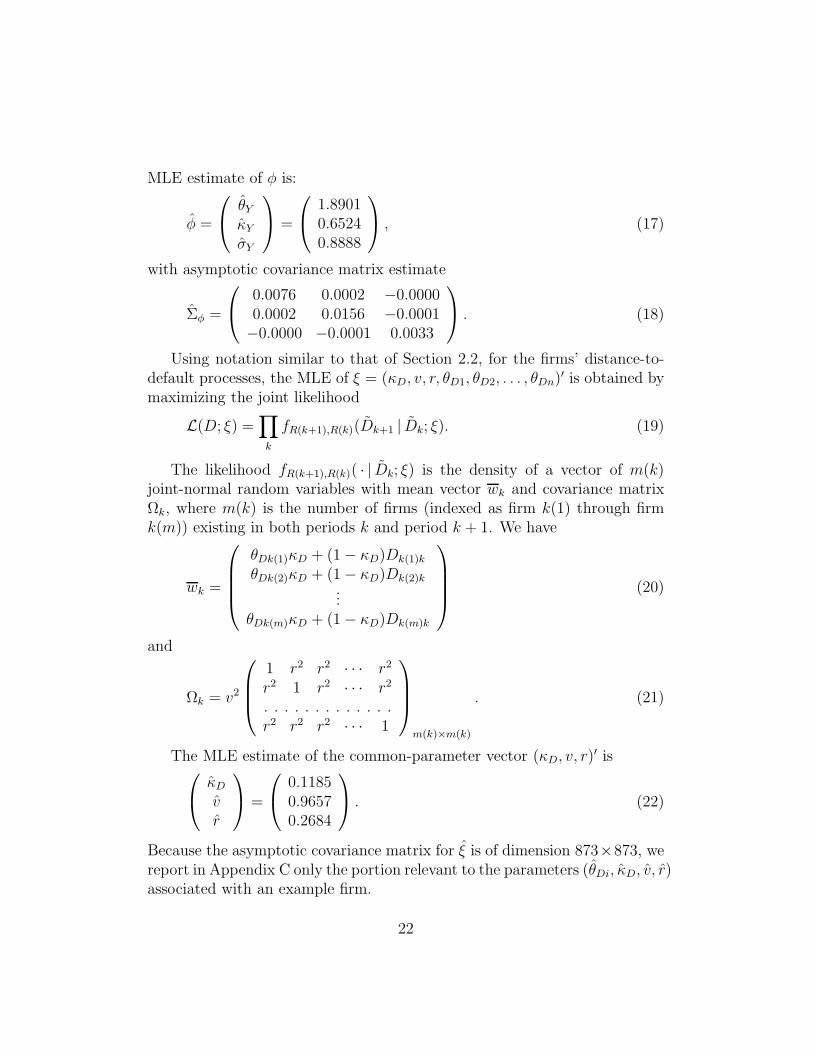
MLE estimate of φ is:

φ =

θYκYσY

=

1.89010.65240.8888

, (17)

with asymptotic covariance matrix estimate

Σφ =

0.0076 0.0002 −0.00000.0002 0.0156 −0.0001−0.0000 −0.0001 0.0033

. (18)

Using notation similar to that of Section 2.2, for the firms’ distance-to-default processes, the MLE of ξ = (κD, v, r, θD1, θD2, . . . , θDn)

′ is obtained bymaximizing the joint likelihood

L(D; ξ) =∏

k

fR(k+1),R(k)(Dk+1 | Dk; ξ). (19)

The likelihood fR(k+1),R(k)( · | Dk; ξ) is the density of a vector of m(k)joint-normal random variables with mean vector wk and covariance matrixΩk, where m(k) is the number of firms (indexed as firm k(1) through firmk(m)) existing in both periods k and period k + 1. We have

wk =

θDk(1)κD + (1 − κD)Dk(1)k

θDk(2)κD + (1 − κD)Dk(2)k...

θDk(m)κD + (1 − κD)Dk(m)k

(20)

and

Ωk = v2

1 r2 r2 · · · r2

r2 1 r2 · · · r2

. . . . . . . . . . . . .r2 r2 r2 · · · 1

m(k)×m(k)

. (21)

The MLE estimate of the common-parameter vector (κD, v, r)′ is

κDvr

=

0.11850.96570.2684

. (22)

Because the asymptotic covariance matrix for ξ is of dimension 873×873, wereport in Appendix C only the portion relevant to the parameters (θDi, κD, v, r)associated with an example firm.

22

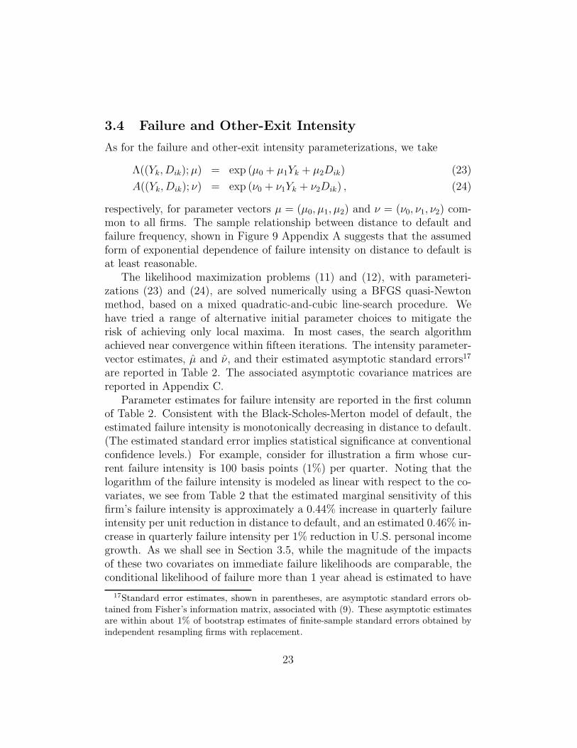
3.4 Failure and Other-Exit Intensity

As for the failure and other-exit intensity parameterizations, we take

Λ((Yk, Dik);µ) = exp (µ0 + µ1Yk + µ2Dik) (23)

A((Yk, Dik); ν) = exp (ν0 + ν1Yk + ν2Dik) , (24)

respectively, for parameter vectors µ = (µ0, µ1, µ2) and ν = (ν0, ν1, ν2) com-mon to all firms. The sample relationship between distance to default andfailure frequency, shown in Figure 9 Appendix A suggests that the assumedform of exponential dependence of failure intensity on distance to default isat least reasonable.

The likelihood maximization problems (11) and (12), with parameteri-zations (23) and (24), are solved numerically using a BFGS quasi-Newtonmethod, based on a mixed quadratic-and-cubic line-search procedure. Wehave tried a range of alternative initial parameter choices to mitigate therisk of achieving only local maxima. In most cases, the search algorithmachieved near convergence within fifteen iterations. The intensity parameter-vector estimates, µ and ν, and their estimated asymptotic standard errors17

are reported in Table 2. The associated asymptotic covariance matrices arereported in Appendix C.

Parameter estimates for failure intensity are reported in the first columnof Table 2. Consistent with the Black-Scholes-Merton model of default, theestimated failure intensity is monotonically decreasing in distance to default.(The estimated standard error implies statistical significance at conventionalconfidence levels.) For example, consider for illustration a firm whose cur-rent failure intensity is 100 basis points (1%) per quarter. Noting that thelogarithm of the failure intensity is modeled as linear with respect to the co-variates, we see from Table 2 that the estimated marginal sensitivity of thisfirm’s failure intensity is approximately a 0.44% increase in quarterly failureintensity per unit reduction in distance to default, and an estimated 0.46% in-crease in quarterly failure intensity per 1% reduction in U.S. personal incomegrowth. As we shall see in Section 3.5, while the magnitude of the impactsof these two covariates on immediate failure likelihoods are comparable, theconditional likelihood of failure more than 1 year ahead is estimated to have

17Standard error estimates, shown in parentheses, are asymptotic standard errors ob-tained from Fisher’s information matrix, associated with (9). These asymptotic estimatesare within about 1% of bootstrap estimates of finite-sample standard errors obtained byindependent resampling firms with replacement.

23

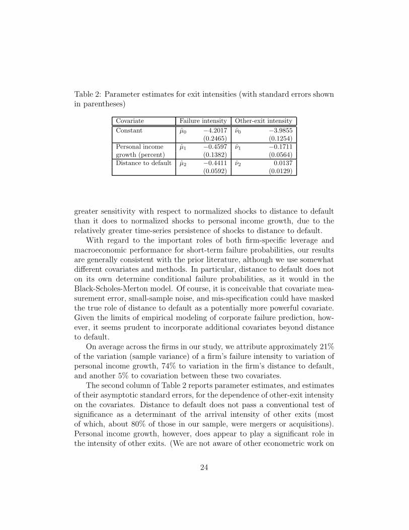
Table 2: Parameter estimates for exit intensities (with standard errors shownin parentheses)

Covariate Failure intensity Other-exit intensity

Constant µ0 −4.2017 ν0 −3.9855(0.2465) (0.1254)

Personal income µ1 −0.4597 ν1 −0.1711growth (percent) (0.1382) (0.0564)Distance to default µ2 −0.4411 ν2 0.0137

(0.0592) (0.0129)

greater sensitivity with respect to normalized shocks to distance to defaultthan it does to normalized shocks to personal income growth, due to therelatively greater time-series persistence of shocks to distance to default.

With regard to the important roles of both firm-specific leverage andmacroeconomic performance for short-term failure probabilities, our resultsare generally consistent with the prior literature, although we use somewhatdifferent covariates and methods. In particular, distance to default does noton its own determine conditional failure probabilities, as it would in theBlack-Scholes-Merton model. Of course, it is conceivable that covariate mea-surement error, small-sample noise, and mis-specification could have maskedthe true role of distance to default as a potentially more powerful covariate.Given the limits of empirical modeling of corporate failure prediction, how-ever, it seems prudent to incorporate additional covariates beyond distanceto default.

On average across the firms in our study, we attribute approximately 21%of the variation (sample variance) of a firm’s failure intensity to variation ofpersonal income growth, 74% to variation in the firm’s distance to default,and another 5% to covariation between these two covariates.

The second column of Table 2 reports parameter estimates, and estimatesof their asymptotic standard errors, for the dependence of other-exit intensityon the covariates. Distance to default does not pass a conventional test ofsignificance as a determinant of the arrival intensity of other exits (mostof which, about 80% of those in our sample, were mergers or acquisitions).Personal income growth, however, does appear to play a significant role inthe intensity of other exits. (We are not aware of other econometric work on

24

the prediction of merger or acquisition.)As a rough diagnostic of the reasonableness of the overall fit of the model,

we compared the actual failure rate in our sample, 0.24% (70 firms out of28,612 firm-quarters) with the average model-implied expected failure rateduring the study period,

∑T−1k=0

∑

i∈R(k)

(

1 − e−λi(k))

∑T

t=0

∑

i∈R(k) 1= 0.23%, (25)

where R(k) is the risk set at the beginning of quarter k, that is the set of firmsoperating at quarter k, and λi(k) is the estimated failure intensity of firm i atquarter k. The denominator of (25) is, as for the actual failure rate, merelythe sample size. We found that the incidence of default in reasonably sizedholdout periods to be too small to allow meaningful judgements regardingout-of-sample performance.

Appendix B reports an estimated model of failure and other-exit intensi-ties that is augmented with two additional covariates: firm-level accountingearnings and firm size. Adding these covariates does not lead to significantchanges, from the basic two-covariate model reported in Table 2, in the coef-ficients representing the dependence of failure intensity on distance to defaultand personal income growth. (It is perhaps noteworthy, however, that withthe addition of earnings and size covariates, the dependence of other-exit in-tensity on distance to default becomes statistically significant at conventionalconfidence levels.)

In the end, we have opted to use the basic two-covariate model for es-timation of term structures of conditional hazard rates. The four-covariatemodel does not offer a better average fit (for example, the associated averageexpected failure probability of the four-covariate model, 0.20no closer thanthe 0.23% estimate of the basic model to the sample failure rate of 0.24%).Firm size and earnings, moreover, are intricately structurally linked in theirtime-series behavior with distance to default, and incorporating the essenceof these structural links into a time-series model for the four covariates seemsfraught with mis-specification risk, not to mention loss of parsimony.18

18See Chava and Jarrow (2002) for additional discussion of the relative importance offirm-specific covariates.

25

3.5 Term Structures of Failure Hazards

We are now in a position to obtain maximum-likelihood estimates, by firm,of the conditional survival and failure probabilities, (1) and (2), for each fu-ture time horizon. For the i-th firm in our sample surviving to a given timet, these conditional probabilities, denoted p(Yt, Dit, s;ψi) and q(Yt, Dit, s;ψi)respectively, depend on the parameter vector ψi = (µ, ν, φ, κD, v, θDi) as-sociated with firm i. Under standard technical conditions, the maximum-likelihood estimators of these conditional probabilities at time horizon s arep(Yt, Dit, s; ψi) and q(Yt, Dit, s; ψi) respectively, where ψi is the maximum-likelihood estimator of ψi.

In order to illustrate the results more meaningfully, we will report theestimated probability density qs(Xt, s; ψi) (partial of q( · ) with respect totime horizon s) of the failure time,19 and the estimated failure hazard rate

H(Yt, Dit, s; ψi) =qs(Yt, Dit, s; ψi)

p(Yt, Dit, s; ψi). (26)

We emphasize that this failure hazard rate at time horizon s conditions onsurvival to time s from both failure and from other forms of exit. (The total-exit hazard rate is, notationally suppressing all arguments of the survivalfunction p( · ) except for the time horizon s, given as usual by −ps(s)/p(s).)

As an illustration, we fix a particular time t, the end of our sample periodat the fourth quarter of 2001, fix a particular firm, General Binding Corpora-tion (GBC), calculate GBC’s estimated conditional term structure of failurehazard rates, and show how that term structure responds to changes to thebusiness-cycle variable Yt and to changes in GBC’s distance to default, Dit.GBC is a natural choice for illustration, given that it has a non-trivial levelof credit risk at time t (with a current Moodys rating of B3, set on December16, 1999), and is a reasonably closely followed firm that existed for 113 quar-ters, most of our sample period. GBC, based in Illinois, is engaged in thedesign, manufacture, and distribution of office equipment, related supplies,and laminating equipment and films. Founded in 1947, GBC first appears inthe Compustat database at the fourth quarter of 1973. At the end of 2002,

19This density is most easily calculated by differentiation through the expectation, as

E(

e−R

t+s

t[λ(u)+α(u)] duλ(t+ s) |Xt

)

, which we compute by Monte-Carlo simulation. We

emphasize that this density is “improper” (integrates over all s to less than one) becauseof other exit events.

26

0 20 40 60 80 100 1200

2

4

6

8

10

12

Quarters from (1973:4)

Dis

tanc

e to

def

ault

Sample Mean: 5.1880 Max: 10.5098 Min: 0.3401 Long−run Mean: 3.9408

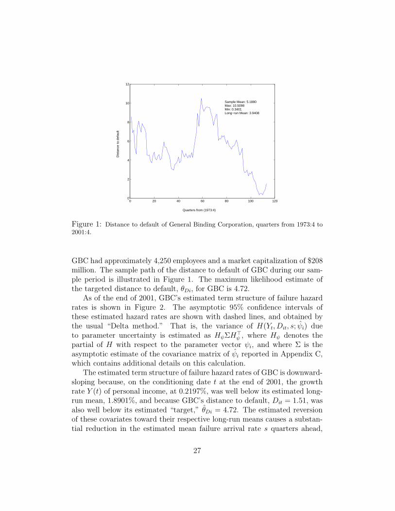
Figure 1: Distance to default of General Binding Corporation, quarters from 1973:4 to2001:4.

GBC had approximately 4,250 employees and a market capitalization of $208million. The sample path of the distance to default of GBC during our sam-ple period is illustrated in Figure 1. The maximum likelihood estimate ofthe targeted distance to default, θDi, for GBC is 4.72.

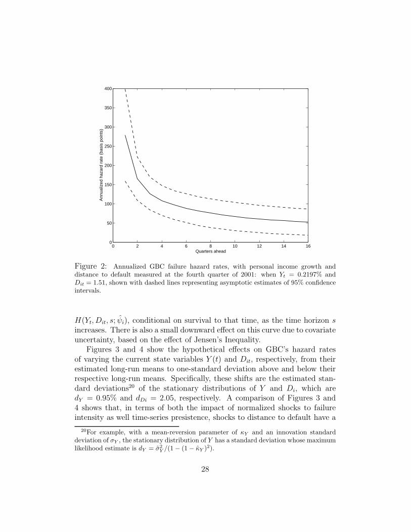
As of the end of 2001, GBC’s estimated term structure of failure hazardrates is shown in Figure 2. The asymptotic 95% confidence intervals ofthese estimated hazard rates are shown with dashed lines, and obtained bythe usual “Delta method.” That is, the variance of H(Yt, Dit, s; ψi) dueto parameter uncertainty is estimated as HψΣH

>ψ , where Hψ denotes the

partial of H with respect to the parameter vector ψi, and where Σ is theasymptotic estimate of the covariance matrix of ψi reported in Appendix C,which contains additional details on this calculation.

The estimated term structure of failure hazard rates of GBC is downward-sloping because, on the conditioning date t at the end of 2001, the growthrate Y (t) of personal income, at 0.2197%, was well below its estimated long-run mean, 1.8901%, and because GBC’s distance to default, Dit = 1.51, wasalso well below its estimated “target,” θDi = 4.72. The estimated reversionof these covariates toward their respective long-run means causes a substan-tial reduction in the estimated mean failure arrival rate s quarters ahead,

27

0 2 4 6 8 10 12 14 160

50

100

150

200

250

300

350

400

Ann

ualiz

ed h

azar

d ra

te (

basi

s po

ints

)

Quarters ahead

Figure 2: Annualized GBC failure hazard rates, with personal income growth anddistance to default measured at the fourth quarter of 2001: when Yt = 0.2197% andDit = 1.51, shown with dashed lines representing asymptotic estimates of 95% confidenceintervals.

H(Yt, Dit, s; ψi), conditional on survival to that time, as the time horizon sincreases. There is also a small downward effect on this curve due to covariateuncertainty, based on the effect of Jensen’s Inequality.

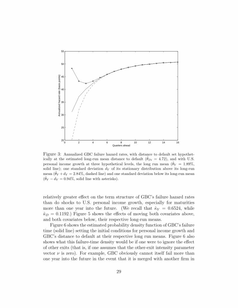
Figures 3 and 4 show the hypothetical effects on GBC’s hazard ratesof varying the current state variables Y (t) and Dit, respectively, from theirestimated long-run means to one-standard deviation above and below theirrespective long-run means. Specifically, these shifts are the estimated stan-dard deviations20 of the stationary distributions of Y and Di, which aredY = 0.95% and dDi = 2.05, respectively. A comparison of Figures 3 and4 shows that, in terms of both the impact of normalized shocks to failureintensity as well time-series presistence, shocks to distance to default have a

20For example, with a mean-reversion parameter of κY and an innovation standarddeviation of σY , the stationary distribution of Y has a standard deviation whose maximumlikelihood estimate is dY = σ2

Y/(1 − (1 − κY )2).

28

0 2 4 6 8 10 12 14 1620

25

30

35

40

45

50

55

Quarters ahead

Ann

ualiz

ed h

azar

d ra

te (

basi

s po

ints

)

Figure 3: Annualized GBC failure hazard rates, with distance to default set hypothet-ically at the estimated long-run mean distance to default (θDi = 4.72), and with U.S.

personal income growth at three hypothetical levels, the long run mean (θY = 1.89%,solid line); one standard deviation dY of its stationary distribution above its long-run

mean (θY +dY = 2.84%, dashed line) and one standard deviation below its long-run mean

(θY − dY = 0.94%, solid line with asterisks).

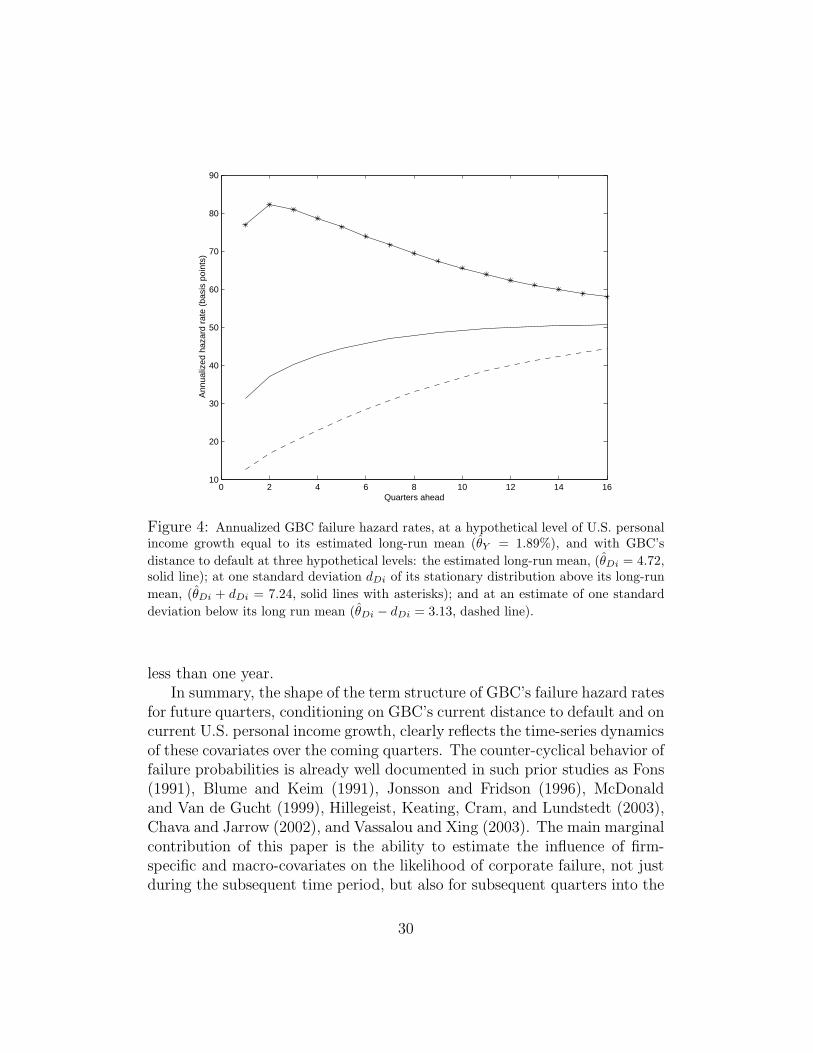
relatively greater effect on the term structure of GBC’s failure hazard ratesthan do shocks to U.S. personal income growth, especially for maturitiesmore than one year into the future. (We recall that κY = 0.6524, whileκD = 0.1192.) Figure 5 shows the effects of moving both covariates above,and both covariates below, their respective long-run means.

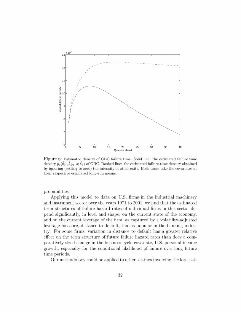
Figure 6 shows the estimated probability density function of GBC’s failuretime (solid line) setting the initial conditions for personal income growth andGBC’s distance to default at their respective long run means. Figure 6 alsoshows what this failure-time density would be if one were to ignore the effectof other exits (that is, if one assumes that the other-exit intensity parametervector ν is zero). For example, GBC obviously cannot itself fail more thanone year into the future in the event that it is merged with another firm in

29

0 2 4 6 8 10 12 14 1610

20

30

40

50

60

70

80

90

Quarters ahead

Ann

ualiz

ed h

azar

d ra

te (

basi

s po

ints

)

Figure 4: Annualized GBC failure hazard rates, at a hypothetical level of U.S. personalincome growth equal to its estimated long-run mean (θY = 1.89%), and with GBC’s

distance to default at three hypothetical levels: the estimated long-run mean, (θDi = 4.72,solid line); at one standard deviation dDi of its stationary distribution above its long-run

mean, (θDi + dDi = 7.24, solid lines with asterisks); and at an estimate of one standard

deviation below its long run mean (θDi − dDi = 3.13, dashed line).

less than one year.In summary, the shape of the term structure of GBC’s failure hazard rates

for future quarters, conditioning on GBC’s current distance to default and oncurrent U.S. personal income growth, clearly reflects the time-series dynamicsof these covariates over the coming quarters. The counter-cyclical behavior offailure probabilities is already well documented in such prior studies as Fons(1991), Blume and Keim (1991), Jonsson and Fridson (1996), McDonaldand Van de Gucht (1999), Hillegeist, Keating, Cram, and Lundstedt (2003),Chava and Jarrow (2002), and Vassalou and Xing (2003). The main marginalcontribution of this paper is the ability to estimate the influence of firm-specific and macro-covariates on the likelihood of corporate failure, not justduring the subsequent time period, but also for subsequent quarters into the

30

0 2 4 6 8 10 12 14 160

20

40

60

80

100

120

Quarters ahead

Ann

ualiz

ed h

azar

d ra

te (

basi

s po

ints

)

Figure 5: Annualized GBC failure hazard rates. Solid line: covariates initialized attheir respective long-run means, θDi = 4.72 and θY = 1.89. Dashed line: covariates eachinitialized one standard deviation (of the respective stationary distributions) above long-run means. Solid line with asterisks: covariates initialized one standard deviation belowlong-run means.

future.

4 Discussion and Additional Applications

This paper offers an econometric method, and an empirical implementationof this method for the U.S. industrial machinery and instruments sector, forestimating the term structure of corporate failure probabilities over multi-ple future periods, conditional on firm-specific and macroeconomic covari-ates. The method, under its probabilistic assumptions, allows one to com-bine traditional duration analysis of the dependence of event intensities ontime-varying covariates with conventional time-series analysis of covariates,in order to obtain maximum-likelihood estimation of multi-period failure

31

0 5 10 15 20 25 30 35 406

7

8

9

10

11

12

13x 10

−4

Quarters ahead

Impl

ied

defa

ult d

ensi

ty

Figure 6: Estimated density of GBC failure time. Solid line: the estimated failure timedensity ps(θY , θDi, s; ψi) of GBC. Dashed line: the estimated failure-time density obtainedby ignoring (setting to zero) the intensity of other exits. Both cases take the covariates attheir respective estimated long-run means.

probabilities.Applying this model to data on U.S. firms in the industrial machinery

and instrument sector over the years 1971 to 2001, we find that the estimatedterm structures of failure hazard rates of individual firms in this sector de-pend significantly, in level and shape, on the current state of the economy,and on the current leverage of the firm, as captured by a volatility-adjustedleverage measure, distance to default, that is popular in the banking indus-try. For some firms, variation in distance to default has a greater relativeeffect on the term structure of future failure hazard rates than does a com-paratively sized change in the business-cycle covariate, U.S. personal incomegrowth, especially for the conditional likelihood of failure over long futuretime periods.

Our methodology could be applied to other settings involving the forecast-

32

ing of discrete events over multiple future periods, in which the time-seriesbehavior of covariates could play a significant role, for example: mortgageprepayment and default, consumer default, initial and seasoned equity offer-ings, merger, acquisition, and the exercise of real timing options, such as theoption to change or abandon a technology.

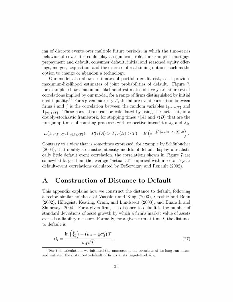
Our model also allows estimates of portfolio credit risk, as it providesmaximum-likelihood estimates of joint probabilities of default. Figure 7,for example, shows maximum likelihood estimates of five-year failure-eventcorrelations implied by our model, for a range of firms distinguished by initialcredit quality.21 For a given maturity T , the failure-event correlation betweenfirms i and j is the correlation between the random variables 1τ(i)<T and1τ(j)<T. These correlations can be calculated by using the fact that, in adoubly-stochastic framework, for stopping times τ(A) and τ(B) that are thefirst jump times of counting processes with respective intensities λA and λB,

E(1τ(A)>T1τ(B)>T) = P (τ(A) > T, τ(B) > T ) = E(

e−R

T

0(λA(t)+λB(t)) dt

)

.

Contrary to a view that is sometimes expressed, for example by Schonbucher(2004), that doubly-stochastic intensity models of default display unrealisti-cally little default event correlation, the correlations shown in Figure 7 aresomewhat larger than the average “actuarial” empirical within-sector 5-yeardefault-event correlations calculated by DeServigny and Renault (2002).

A Construction of Distance to Default

This appendix explains how we construct the distance to default, followinga recipe similar to those of Vassalou and Xing (2003), Crosbie and Bohn(2002), Hillegeist, Keating, Cram, and Lundstedt (2003), and Bharath andShumway (2004). For a given firm, the distance to default is the number ofstandard deviations of asset growth by which a firm’s market value of assetsexceeds a liability measure. Formally, for a given firm at time t, the distanceto default is

Dt =ln(

Vt

Lt

)

+(

µA − 12σ2A

)

T

σA√T

, (27)

21For this calculation, we initiated the macroeconomic covariate at its long-run mean,and initiated the distance-to-default of firm i at its target-level, θDi.

33

0200

400600

8001000

0

200

400

600

800

1000

0.1

0.105

0.11

0.115

0.12

0.125

0.13

Default intensity λi(0)Default intensity λj(0)

Fiv

e-ye

ardef

ault-e

vent

corr

elat

ion

Figure 7: Five-year default-event correlations

where Vt is the market value of the firm’s assets at time t and Lt is a liabilitymeasure, defined below, that is often known in industry practice as the “de-fault point”. Here, µA and σA measure the firm’s mean rate of asset growthand asset volatility, respectively, and T is a chosen time horizon, typicallytaken to be 4 quarters.

The default point Lt, following the standard established by Moodys KMV(see Crosbie and Bohn (2002), as followed by Vassalou and Xing (2003)), ismeasured as the firm’s book measure of short-term debt (“Debt in currentliabilities”, Compustat item 45), plus one half of its long-term debt (item51), based on its quarterly accounting balance sheet. If these accountingmeasures of debt are missing in the Compustat quarterly file, but availablein the annual file, we replace the missing data with the associated annualdebt data (Compustat items 34 and item 9 for short-term and long termdebt, respectively). Of 28, 612 firm-quarters in our sample, there are 3, 086firm-quarters in which we use annual debt data to approximate quarterlydebt data in this way.

34

We estimate the assets Vt and volatility σA according to a call-optionpricing formula, following the theory of Merton (1974) and Black and Scholes(1973), under which equity may be viewed as a call option on the value of afirm’s assets, Vt. In this setting, the market value of equity, Wt, is the optionprice at strike Lt and time T to expiration.

We take the initial asset value Vt to be the sum of Wt (end-of-quarterstock price times number of shares outstanding, from the CRSP database)and the book value of total debt (the sum of short-term debt and long-termdebt from Compustat). We take the risk-free return r to be the one-year T-bill rate. We solve for the asset value Vt and asset volatility σA by iterativelyapplying the equations:

Wt = VtΦ(d1) − Lte−rTΦ(d2) (28)

σA = sdev (ln(Vt) − ln(Vt−1)) , (29)

where

d1 =ln(

Vt

Lt

)

+ (r + 12σ2A)T

σA√T

, (30)

d2 = d1 − σA√T , and Φ( · ) is the standard-normal cumulative distribution

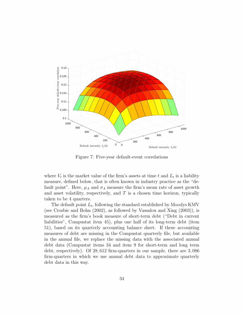
function, and sdev( · ) denotes sample standard deviation. Equation (28) isthe call-option pricing formula of Black and Scholes (1973), allowing, through(29), an estimate of the asset volatility σA. For simplicity, by using (29), weavoided the calculation of the volatility implied by the option pricing model(See Crosbie and Bohn (2002) and Hillegeist, Keating, Cram, and Lundstedt(2003) for this alternative approach), but instead estimated σA as the samplestandard deviation of the time series of asset-value growth, ln(Vt)− ln(Vt−1).A histogram22 of our sample of distances to default is provided in Figure 8.

Our construction of distance to default has the property that, in thetheoretical setting of Merton (1974), a firm whose current distance to defaultisD has a conditional probability (given all available information) of failure inone year of Φ(−D), where Φ is the cumulative standard-normal distributionfunction. Figure 9 shows the average realtionship in our sample betweendistance to default and failure rate. For the purpose of this figure, distanceto default is “bucketed” into intervals of length 0.25. The denominator for

22Of all 28, 612 firm-quarters, four had distances to default larger than 40. These arenot shown in Figure 8.

35

−5 0 5 10 15 20 25 30 35 400

200

400

600

800

1000

1200

1400

1600

Distance to Default

Fre

quen

cy o

f Firm

−qu

arte

rs

Figure 8: Histogram of distance to default for firm-quarters in the sample.

a given bucket is the number of firm-quarters with distance to default inthe associated interval; the numerator is the number of failures from thatbucket within the subsequent quater. We did not include in Figure 9 thosebuckets with distances to default of less than −2, which constitutes 0.8% ofthe firm-quarters in our sample. Figure 9 illustrates an average relationshipbetween distance to default and failure frequency that is roughly consistentwith our assumption that failure intensity depends exponentially on distanceto default, fixing other covariates.

B Four-Covariate Intensity Model

This appendix provides coefficient estimates for a model of failure and mergerintensities based on the covariates listed in Table 1.

Instead of assuming (23) and (24), we specify failure intensity and other-exit intensity to be the form:

Λ((Yk, Dik, Rik, Sik);µ) = eµ0+µ1Yk+µ2Dik+µ3Rik+µ4Sik (31)

A((Yk, Dik, Rik, Sik); ν) = eν0+ν1Yk+ν2Dik+ν3Rik+ν4Sik , (32)

where Rik is the earnings (relative to assets) of firm i in quarter k, and Sikis the size of firm i in quarter k, as explained in Section 3.2. Maximizing

36

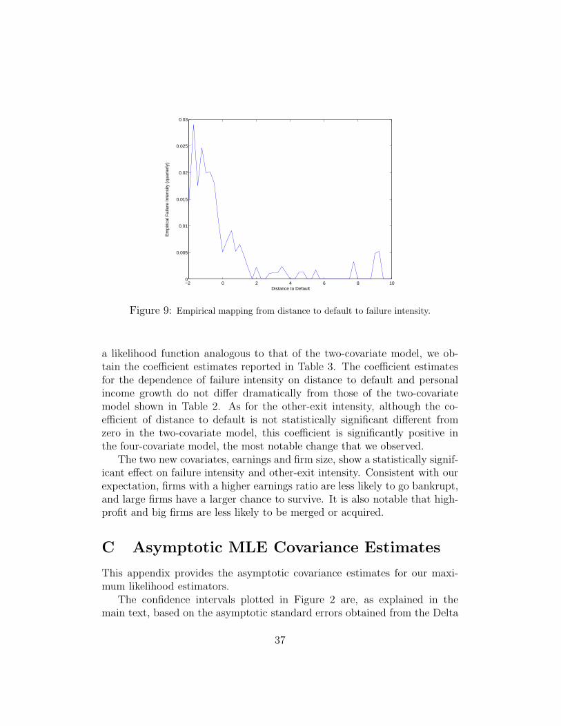
−2 0 2 4 6 8 100

0.005

0.01

0.015

0.02

0.025

0.03

Distance to Default

Em

piric

al F

ailu

re In

tens

ity (

quar

terly

)

Figure 9: Empirical mapping from distance to default to failure intensity.

a likelihood function analogous to that of the two-covariate model, we ob-tain the coefficient estimates reported in Table 3. The coefficient estimatesfor the dependence of failure intensity on distance to default and personalincome growth do not differ dramatically from those of the two-covariatemodel shown in Table 2. As for the other-exit intensity, although the co-efficient of distance to default is not statistically significant different fromzero in the two-covariate model, this coefficient is significantly positive inthe four-covariate model, the most notable change that we observed.

The two new covariates, earnings and firm size, show a statistically signif-icant effect on failure intensity and other-exit intensity. Consistent with ourexpectation, firms with a higher earnings ratio are less likely to go bankrupt,and large firms have a larger chance to survive. It is also notable that high-profit and big firms are less likely to be merged or acquired.

C Asymptotic MLE Covariance Estimates

This appendix provides the asymptotic covariance estimates for our maxi-mum likelihood estimators.

The confidence intervals plotted in Figure 2 are, as explained in themain text, based on the asymptotic standard errors obtained from the Delta

37

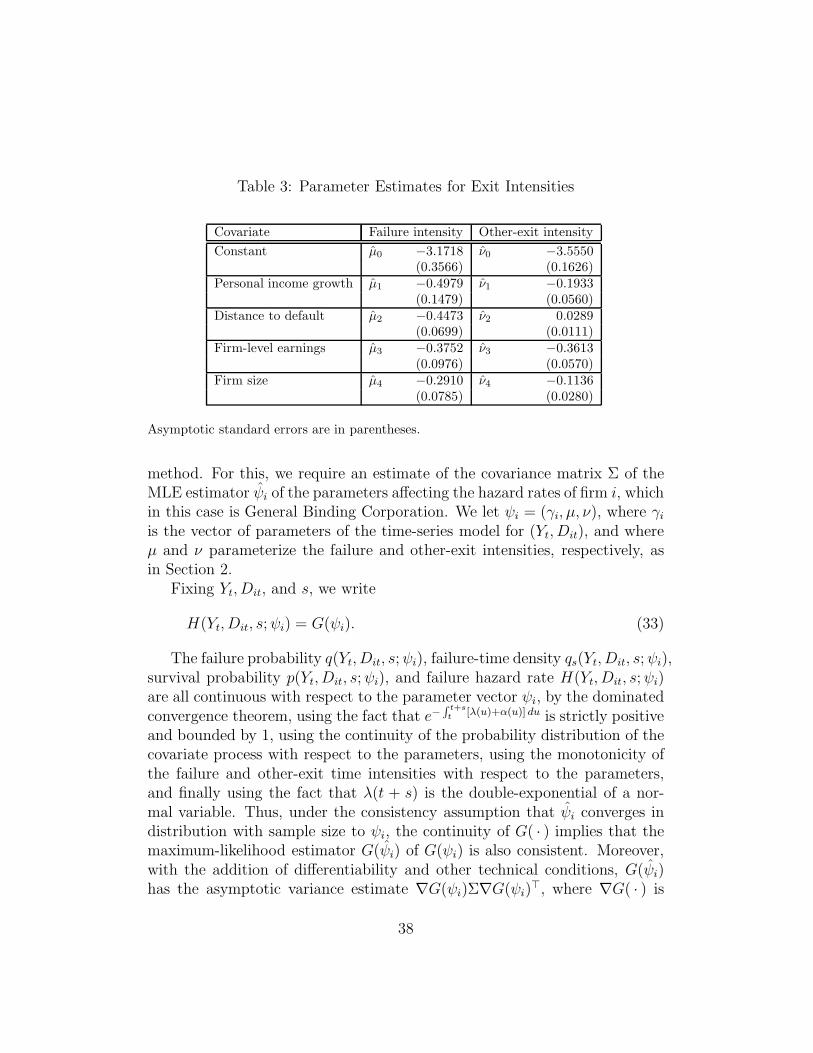
Table 3: Parameter Estimates for Exit Intensities

Covariate Failure intensity Other-exit intensity

Constant µ0 −3.1718 ν0 −3.5550(0.3566) (0.1626)

Personal income growth µ1 −0.4979 ν1 −0.1933(0.1479) (0.0560)

Distance to default µ2 −0.4473 ν2 0.0289(0.0699) (0.0111)

Firm-level earnings µ3 −0.3752 ν3 −0.3613(0.0976) (0.0570)

Firm size µ4 −0.2910 ν4 −0.1136(0.0785) (0.0280)

Asymptotic standard errors are in parentheses.

method. For this, we require an estimate of the covariance matrix Σ of theMLE estimator ψi of the parameters affecting the hazard rates of firm i, whichin this case is General Binding Corporation. We let ψi = (γi, µ, ν), where γiis the vector of parameters of the time-series model for (Yt, Dit), and whereµ and ν parameterize the failure and other-exit intensities, respectively, asin Section 2.

Fixing Yt, Dit, and s, we write

H(Yt, Dit, s;ψi) = G(ψi). (33)

The failure probability q(Yt, Dit, s;ψi), failure-time density qs(Yt, Dit, s;ψi),survival probability p(Yt, Dit, s;ψi), and failure hazard rate H(Yt, Dit, s;ψi)are all continuous with respect to the parameter vector ψi, by the dominatedconvergence theorem, using the fact that e−

R

t+s

t[λ(u)+α(u)] du is strictly positive

and bounded by 1, using the continuity of the probability distribution of thecovariate process with respect to the parameters, using the monotonicity ofthe failure and other-exit time intensities with respect to the parameters,and finally using the fact that λ(t + s) is the double-exponential of a nor-mal variable. Thus, under the consistency assumption that ψi converges indistribution with sample size to ψi, the continuity of G( · ) implies that themaximum-likelihood estimator G(ψi) of G(ψi) is also consistent. Moreover,with the addition of differentiability and other technical conditions, G(ψi)has the asymptotic variance estimate ∇G(ψi)Σ∇G(ψi)

>, where ∇G( · ) is

38

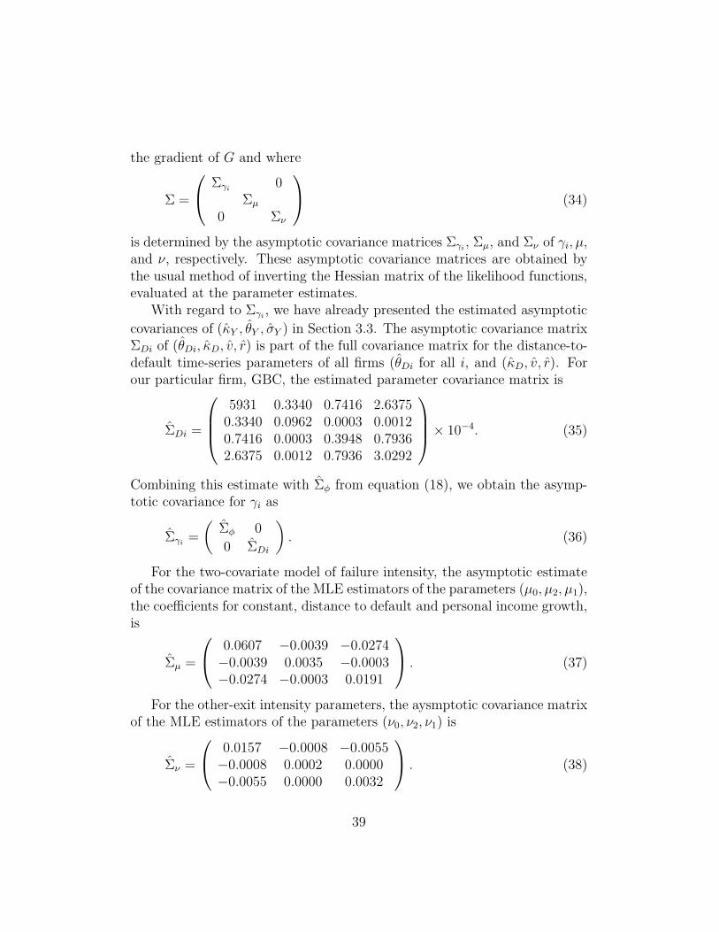
the gradient of G and where

Σ =

Σγi0

Σµ

0 Σν

(34)

is determined by the asymptotic covariance matrices Σγi, Σµ, and Σν of γi, µ,

and ν, respectively. These asymptotic covariance matrices are obtained bythe usual method of inverting the Hessian matrix of the likelihood functions,evaluated at the parameter estimates.

With regard to Σγi, we have already presented the estimated asymptotic

covariances of (κY , θY , σY ) in Section 3.3. The asymptotic covariance matrixΣDi of (θDi, κD, v, r) is part of the full covariance matrix for the distance-to-default time-series parameters of all firms (θDi for all i, and (κD, v, r). Forour particular firm, GBC, the estimated parameter covariance matrix is

ΣDi =

5931 0.3340 0.7416 2.63750.3340 0.0962 0.0003 0.00120.7416 0.0003 0.3948 0.79362.6375 0.0012 0.7936 3.0292

× 10−4. (35)

Combining this estimate with Σφ from equation (18), we obtain the asymp-totic covariance for γi as

Σγi=

(

Σφ 0

0 ΣDi

)

. (36)

For the two-covariate model of failure intensity, the asymptotic estimateof the covariance matrix of the MLE estimators of the parameters (µ0, µ2, µ1),the coefficients for constant, distance to default and personal income growth,is

Σµ =

0.0607 −0.0039 −0.0274−0.0039 0.0035 −0.0003−0.0274 −0.0003 0.0191

. (37)

For the other-exit intensity parameters, the aysmptotic covariance matrixof the MLE estimators of the parameters (ν0, ν2, ν1) is

Σν =

0.0157 −0.0008 −0.0055−0.0008 0.0002 0.0000−0.0055 0.0000 0.0032

. (38)

39

References

Allen, L. and A. Saunders (2002). A Survey of Cyclical Effects in CreditRisk Measurement Models. mimeo, Stern School of Business, New YorkUniversity.

Altman, E. I. (1968). Financial Ratios, Discriminant Analysis, and thePrediction of Corporate Bankruptcy. Journal of Finance 23, 589–609.

Amemiya, T. (1985). Advanced Econometrics. Cambridge, Massachusetts:Harvard University Press.

Andersen, P. K., O. Borgan, R. D. Gill, and N. Keiding (1992). StatisticalModels Based on Counting Processes. New York: Springer-Verlag.

Beaver, B. (1966). Financial Ratios as Predictors of Failure. EmpiricalResearch in Accounting: Selected Studies, Supplment to Journal of Ac-counting Research Autumn, 91–101.

Beaver, B. (1968a). Alternative Accounting Measures as Predictors of Fail-ure. Accounting Review January, 113–122.

Beaver, B. (1968b). Market Prices, Financial Ratios, and the Predictionof Failure. Journal of Accounting Research Autumn, 170–192.

Behar, R. and K. Nagpal (1999). Dynamics of Rating Transition. WorkingPaper, Standard and Poor’s.

Berman, S. M. and H. Frydman (1999). Parametric Estimation of HazardFunctions with Stochastic Covariate Processes. Sankhya, Series A 61,174–188.

Bharath, S. and T. Shumway (2004). Forecasting Default with the KMV-Merton Model. Working Paper, University of Michigan.

Black, F. and M. Scholes (1973). The Pricing of Options and CorporateLiabilities. Journal of Political Economy 81, 637–654.

Blume, M. and D. Keim (1991). Realized Returns and Volatility of Low-Grade Bonds: 1977-1989. Journal of Finance 46, 49–74.

Chava, S. and R. Jarrow (2002). Bankruptcy Prediction with IndustryEffects. Working Paper, Cornell University.

Collin-Dufresne, P. and R. Goldstein (2001). Do Credit Spreads ReflectStationary Leverage Ratios? Reconciling Structural and Reduced-Form Frameworks. Journal of Finance 56, 1929–1958.

40

Cox, D. R. and V. Isham (1980). Point Processes. New York: Chapmanand Hall.

Cox, D. R. and D. Oakes (1984). Analysis of Survival Data. New York:Chapman and Hall.

Crosbie, P. J. and J. R. Bohn (2002). Modeling Default Risk. TechnicalReport, KMV, LLC.

Daley, D. J. and D. Vere-Jones (1988). An Introduction to the Theory ofPoint Processes. New York: Springer.

Das, S. R., D. Duffie, and N. Kapadia (2004). Common Failings: How Cor-porate Defaults are Correlated. Working Paper, Stanford University.

DeServigny, A. and O. Renault (2002). Default Correlation: EmpiricalEvidence. Working Paper, Standard and Poor’s.

Duffie, D. (2001). Dynamic Asset Pricing Theory (Third edition). Prince-ton, New Jersey: Princeton University Press.

Duffie, D., D. Filipovic, and W. Schachermayer (2003). Affine Processesand Applications in Finance. Annals of Applied Probability 13, 984–1053.

Duffie, D. and D. Lando (2001). Term Structures of Credit Spreads withIncomplete Accounting Information. Econometrica 69, 633–664.

Duffie, D., J. Pan, and K. Singleton (2000). Transform Analysis and AssetPricing for Affine Jump-Diffusions. Econometrica 68, 1343–1376.

Duffie, D. and K. Singleton (2003). Credit Risk. Princeton, New Jersey:Princeton University Press.

Engle, R. F. and J. R. Russell (1998). Autoregressive Conditional Dura-tion: A New Model for Irregularly Spaced Transaction Data. Econo-metrica 66, 1127–1162.

Engle, R. F. and J. R. Russell (2002). Econometric Analysis of Discrete-Valued Irregularly-Spaced Financial Transactions Data. Working Pa-per, University of California, San Diego.

Fama, E. and K. French (2004). New Lists: Fundamentals and SurvivalRates. Journal of Financial Economics 73, 229–269.

Fisher, E., R. Heinkel, and J. Zechner (1989). Dynamic Capital StructureChoice: Theory and Tests. Journal of Finance 44, 19–40.

41

Fons, J. (1991). An Approach to Forecasting Default Rates. Working Pa-per, Moody’s Investors Services.

Helwege, J. and P. Kleiman (1997). Understanding Aggregate DefaultRates of High Yield Bonds. Journal of Fixed Income 7, 55–62.

Hillegeist, S. A., E. K. Keating, D. P. Cram, and K. G. Lundstedt (2003).Assessing the Probability of Bankruptcy. Working Paper, NorthwesternUniversity.

Jones, F. (1987). Current Techniques in Bankruptcy Prediction. Journalof Accounting Literature 6, 131–164.

Jonsson, J. and M. Fridson (1996, June). Forecasting Default Rates onHigh-Yield Bonds. The Journal of Fixed Income, 69–77.

Kalbfleisch, J. and R. Prentice (2002). The Statistical Analysis of FailureTime Data (Second edition). Hoboken, New Jersey: John Wiley &Sons.

Karr, A. (1991). Point Processes and Statistical Inference (Second edition).New York: Marcel Dekker.

Kavvathas, D. (2001). Estimating Credit Rating Transition Probabilitiesfor Corporate Bonds. Working paper, University of Chicago.

Kealhofer, S. (2003). Quantifying Credit Risk I: Default Prediction. Fi-nancial Analysts Journal , January–February, 30–44.

Keenan, S. C., J. Sobehart, and D. T. Hamilton (1999). Predicting DefaultRates: A Forecasting Model For Moody’s Issuer-Based Default Rates.Working Paper, Moody’s Investors Services.

Lancaster, T. (1990). The Econometric Analysis of Transition Data. NewYork: Cambridge University Press.

Lando, D. and T. Skødeberg (2002). Analyzing Rating Transitions andRating Drift with Continuous Observations. Journal of Banking andFinance 26, 423–444.

Lane, W. R., S. W. Looney, and J. W. Wansley (1986). An Applicationof the Cox Proportional Hazards Model to Bank Failure. Journal ofBanking and Finance 10, 511–531.

Lee, S. H. and J. L. Urrutia (1996). Analysis and Prediction of Insolvencyin the Property-Liability Insurance Industry: A Comparison of Logitand Hazard Models. The Journal of Risk and Insurance 63, 121–130.

42

Leland, H. (1994). Corporate Debt Value, Bond Covenants, and OptimalCapital Structure. Journal of Finance 49, 1213–1252.

Leland, H. (1998). Agency Costs, Risk Manamgement, and Capital Struc-ture. Journal of Finance 53, 1213–1242.

McDonald, C. G. and L. M. Van de Gucht (1999). High-Yield Bond Defaultand Call Risks. Review of Economics and Statistics 81, 409–419.

Merton, R. C. (1974). On the Pricing of Corporate Debt: The Risk Struc-ture of Interest Rates. Journal of Finance 29, 449–470.

Meyer, B. D. (1990). Unemployment Insurance and Unemployment Spells.Econometrica 58, 757–782.

Miller, R. (1981). Survival Analysis. New York: John Wiley & Sons.

Nickell, P., W. Perraudin, and S. Varotto (2000). Stability of Rating Tran-sitions. Journal of Banking and Finance 24, 203–227.

Ohlson, J. (1980). Financial Ratios and the Probabilistic Prediction ofBankruptcy. Journal of Accounting Research 19, 109–131.

Pesaran, M. H., T. Schuermann, B.-J. Treutler, and S. M. Weiner (2003).Macroeconomic Dynamics and Credit Risk: A Global Perspective. Un-published working paper. Wharton School, Federal Reserve Bank, NewYork.

Philosophov, L. and V. Philiosophov (2002). Corporate Bankruptcy Prog-nosis: An Attempt at a Combined Prediction of the Bankruptcy Eventand Time Interval of its Occurrence. International Review of FinancialAnalysis 11, 375–406.

Protter, P. (1990). Stochastic Integration and Differential Equations. NewYork: Springer-Verlag.

Schonbucher, P. (2004). Frailty Models, Contagion, and Information Ef-fects. Working Paper, ETH, Zurich.

Shumway, T. (2001). Forecasting Bankruptcy More Accurately: A SimpleHazard Model. Journal of Business 74, 101–124.

Therneau, T. M. and P. M. Grambsch (2000). Modeling Survival Data:Extending the Cox Model. New York: Springer-Verlag.

Vassalou, M. and Y. Xing (2003). Default Risk in Equity Returns. WorkingPaper, Columbia University, forthcoming, Journal of Finance.

43

Whalen, G. (1991). A Proportional Hazards Model of Bank Failure: AnExamination of its Usefulness as an Early Warning Model Tool. InFederal Reserve Bank of Cleveland Economic Review, pp. 21–31. 1991.

Wheelock, D. C. and P. W. Wilson (2000). Why Do Banks Disappear?The Determinants of U.S. Bank Failures and Acquisitions. Review ofEconomics and Statistics 82, 127–138.

Wilson, T. (1997a). Portfolio Credit Risk, I. RISK 10, September, 111–117.

Wilson, T. (1997b). Portfolio Credit Risk, I. RISK 10, October, 56–61.

44