NBER WORKING PAPER SERIES

LONG-RUN RISKS AND FINANCIAL MARKETS

Ravi Bansal

Working Paper 13196http://www.nber.org/papers/w13196

NATIONAL BUREAU OF ECONOMIC RESEARCH1050 Massachusetts Avenue

Cambridge, MA 02138June 2007

The views expressed herein are those of the author(s) and do not necessarily reflect the views of theNational Bureau of Economic Research.

© 2007 by Ravi Bansal. All rights reserved. Short sections of text, not to exceed two paragraphs, maybe quoted without explicit permission provided that full credit, including © notice, is given to the source.

Long-Run Risks and Financial MarketsRavi BansalNBER Working Paper No. 13196June 2007JEL No. E0,E44,G0,G1,G12

ABSTRACT

The recently developed long-run risks asset pricing model shows that concerns about long-run expectedgrowth and time-varying uncertainty (i.e., volatility) about future economic prospects drive asset prices.These two channels of economic risks can account for the risk premia and asset price fluctuations.In addition, the model can empirically account for the cross-sectional differences in asset returns. Hence,the long-run risks model provides a coherent and systematic framework for analyzing financial markets.

Ravi BansalFuqua School of BusinessDuke University1 Towerview DriveDurham, NC 27708and NBERravi.bansal@duke.edu

1 Introduction

From the perspective of theoretical models, several key features of asset markets are puz-

zling. Among others, these puzzling features include the level of equity premium (see Mehra

and Prescott, 1985), asset price volatility (see Shiller, 1981), and the large cross-sectional

differences in average returns across equity portfolios such as value and growth portfolios. In

bond and foreign exchange markets, the violations of the expectations hypothesis (see Fama

and Bliss, 1987; Fama, 1984) and the ensuing return predictability is quantitatively difficult

to explain. What risks and investor concerns can provide a unified explanation for these

asset market facts? One potential explanation of all these anomalies is the long-run risks

model developed in Bansal and Yaron (2004) (henceforth BY). In this model, fluctuations

in the long-run growth prospects of the economy and the time-varying level of economic un-

certainty (consumption or output volatility) drive financial markets. Recent work indicates

that many of the asset prices anomalies are a natural outcome of these channels developed in

BY. In this article I explain the key mechanisms in the BY model that enable it to account

for the asset market puzzles.

In the BY model, the first economic channel relates to expected growth: Consumption

and dividend growth rates contain a small long-run component in the mean. That is, cur-

rent shocks to expected growth alter expectations about future economic growth not only

for short horizons but also for the very long run. The second channel pertains to varying

economic uncertainty: Conditional volatility of consumption is time varying. Fluctuations in

consumption volatility lead to time variation in risk premia. Agents fear adverse movements

in the long-run growth and volatility components because they lower equilibrium consump-

tion, wealth, and asset prices. This makes holding equity quite risky, leading to high risk

compensation in equity markets.

The preferences developed in Epstein and Zin (1989) play an important role in the long-

run risks model. These preferences allow for a separation between risk aversion and intertem-

poral elasticity of substitution (IES) of investors: The magnitude of the risk aversion relative

to the reciprocal of the IES determines whether agents prefer early or late resolution of un-

certainty regarding the consumption path. In the BY model, agents prefer early resolution

of uncertainty; that is, risk aversion is larger than the reciprocal of the IES. This ensures

that the compensation for long-run expected growth risk is positive. The resulting model

has three distinct sources of risks that determine the risk premia: short-run, long-run, and

1

consumption volatility risks. In the traditional power utility model, only the first risk source

carries a distinct risk price and the other two risks have zero risk compensation. Separate

risk compensation for shocks to consumption volatility and expected consumption growth is

a novel feature of the BY model relative to earlier asset pricing models.

To derive model implications for asset prices, the preference parameters are calibrated.

The calibrated magnitude of the risk aversion and the IES is an empirical issue. Hansen and

Singleton (1982), Attanasio and Weber (1989), and Vissing-Jorgensen and Attanasio (2003)

estimate the IES to be well in excess of 1. Hall (1988) and Campbell (1999), on the other

hand, estimate its value to be well below 1. BY show that even if the population value of

the IES is larger than 1, the estimation methods used by Hall would measure the IES to

be close to zero. That is, in the presence of time-varying consumption volatility, there is a

severe downward bias in the point estimates of IES. Using the data from financial markets,

Bansal, Khatchatrian, and Yaron (2005) and Bansal and Shaliastovich (2007) provide further

evidence on the magnitude of the IES.

Different techniques are employed to provide empirical and theoretical support for the

existence of long-run components in consumption and dividends. Whereas BY calibrate pa-

rameters to match the annual moments of consumption and dividend growth rates, Bansal,

Gallant, and Tauchen (2007) and Bansal, Kiku, and Yaron (2006) formally test the model

using the efficient and generalized method of moments, respectively. Using multivariate anal-

ysis Hansen, Heaton, and Li (2005) and Bansal, Kiku, and Yaron (2006) present evidence

for long-run components in consumption growth. Colacito and Croce (2006) also provide

statistical support for the long-run components in consumption data for the United States

and other developed economies. Lochstoer and Kaltenbrunner (2006) provide a production-

based motivation for long-run risks in consumption. They show that in a standard produc-

tion economy, where consumption is endogenous, the consumption growth process contains

a predictable long-run component similar to that in the BY model. There is considerable

support for the volatility channel as well. Bansal, Khatchatrian, and Yaron (2005) show that

consumption volatility is time varying and that its current level predicts future asset valu-

ations (price-dividend ratio) with a significantly negative projection coefficient; this implies

that asset markets dislike economic uncertainty. Exploiting the BY uncertainty channel,

Lettau, Ludvigson, and Wachter (2007) provide interesting market premium implications of

the low-frequency decline in consumption volatility.

BY show that their long-run risks model can explain the risk-free rate, the level of

2

the equity premium, asset price volatility, and many of the return and dividend growth

predictability dimensions that have been characterized in earlier work. The time-varying

volatility in consumption is important to capture some of the economic outcomes that relate

to time-varying risk premia.

The arguments presented in their work also have immediate implications for the cross-

sectional differences in mean returns across assets. Bansal, Dittmar, and Lundblad (2002 and

2005) show that the systematic risks across firms should be related to the systematic long-

run risks in firms’ cash flows that investors receive. Firms whose expected cash-flow (profits)

growth rates move with the economy are more exposed to long-run risks and hence should

carry higher risk compensation. These authors develop methods to measure the exposure

of cash flows to long-run risks, and show that these cash flow betas can account for the

differences in risk premia across assets. They show that the high book-to-market portfolio

(i.e., value portfolio) has a larger long-run risks beta relative to the low book-to-market

portfolio (i.e., growth portfolio). Hence, the high mean return of value firms relative to

growth firms is not puzzling. The Bansal, Dittmar, and Lundblad (2002 and 2005) evidence

supports a long-run risks explanation for the cross-sectional differences in mean returns.

Several recent papers use the BY long-run risks model to address a rich array of asset

market questions; among others, these include Kiku (2006), Colacito and Croce (2006),

Lochstoer and Kaltenbrunner (2006), Chen, Collin-Dufresne, and Goldstein (2006), Chen

(2006), Eraker (2006), Piazzesi and Schneider (2005), and Bansal and Shaliastovich (2007).

Kiku (2006) shows that the long-run risks model can account for the violations of the capital

asset pricing model (CAPM) and consumption CAPM (C-CAPM) in explaining the cross-

sectional differences in mean returns. Further, the model can capture the entire transition

density of value or growth returns, which underscores the importance of long-run risks in

accounting for equity markets’ behavior. Eraker (2006) and Piazzesi and Schneider (2005)

consider the implications of the model for the risk premia on U.S. Treasury bonds and show

how to account for some of the average premium puzzles in the term structure literature.

Colacito and Croce (2006) extend the long-run risks model to a two-country setup and

explain the issues about international risk sharing and exchange rate volatility. Bansal

and Shaliastovich (2007) show that the long-run risks model can simultaneously account

for the behavior of equity markets, yields, and foreign exchange and explain the nature of

predictability and violations of the expectations hypothesis in foreign exchange and Treasury

markets. Chen, Collin-Dufresne, and Goldstein (2006) and Chen (2006) analyze the ability

3

of the long-run risks model to explain the credit spread and leverage puzzles of the corporate

sector.

Hansen, Heaton, and Li (2005) consider a long-run risks model with a unit IES speci-

fication. Using different methods to measure long-run risks exposures of portfolios sorted

by book-to-market ratio, they find, as in Bansal, Dittmar, and Lundblad (2005), that these

alternative long-run risk measures do line-up in the cross-section with the average returns.

They further show that the measurement of long-run risks can be sensitive to the economet-

ric methods used. Hansen and Sargent (2006) highlight the interesting implications of robust

decision-making for risks in financial markets when the representative agent entertains the

long-run risks model as a baseline description of the economy.

The above results indicate that the long-run risks model can go a long way toward

providing an explanation for many of the key features of asset markets.

The remainder of the article has three sections. The next section reviews the long-run

risks model of Bansal and Yaron (2004). The third section discusses the empirical evidence

of the model and, in particular, its implications for the equity, bond, and currency markets.

The final section concludes.

4

2 Long-Run Risks Model

2.1 Preferences and the Environment

Consider a representative agent with the following Epstein and Zin (1989) recursive prefer-

ences,

Ut = {(1 − δ)C1−γθ

t + δ(Et[U1−γt+1 ])1/θ}

θ1−γ ,

where the rate of time preference is determined by δ, with 0 < δ < 1. The parameter θ is

determined by the risk aversion and the IES — specifically,

θ ≡1 − γ

1 − 1ψ

,

γ ≥ 0 is the risk aversion parameter and ψ ≥ 0 is the IES. The sign of θ is determined by

the magnitudes of the risk aversion and the elasticity of substitution. In particular, if ψ > 1

and γ > 1, then θ will be negative. Note that, when θ = 1 (that is, γ = 1ψ

), one obtains the

standard case of expected utility.

As is pointed out in Epstein and Zin (1989), when risk aversion equals the reciprocal

of IES (expected utility), the agent is indifferent to the timing of the resolution of the

uncertainty of the consumption path. When risk aversion exceeds (is less than) the reciprocal

of IES, the agent prefers early (late) resolution of uncertainty of consumption path. In the

long-run risks model, agents prefer early resolution of the uncertainty of the consumption

path.

The period budget constraint for the agent with wealth Wt and consumption Ct at date

t, is

Wt+1 = (Wt − Ct)Ra,t+1. (1)

Ra,t+1 = Wt+1

(Wt−Ct)is the return on the aggregate portfolio held by the agent. As in Lucas

(1978), we normalize the supply of all equity claims to be 1 and the risk-free asset to be in

zero net supply. In equilibrium, aggregate dividends in the economy (which also include any

claims to labor income) equals aggregate consumption of the representative agent. Given a

process for aggregate consumption, the return on the aggregate portfolio corresponds to the

return on an asset that delivers aggregate consumption as its dividends each time period.

The logarithm of the intertemporal marginal rate of substitution (IMRS), mt+1, for these

5

preferences (Epstein and Zin, 1989) is

mt+1 = θ log δ −θ

ψgt+1 + (θ − 1)ra,t+1 (2)

and the asset pricing restriction on any continuous return ri,t+1 is

Et

[

exp(θ log δ −θ

ψgt+1 + (θ − 1)ra,t+1 + ri,t+1)

]

= 1, (3)

where gt+1 equals log(Ct+1/Ct) — the log growth rate of aggregate consumption. The return,

ra,t+1, is the log of the return (i.e., continuous return) on an asset which delivers aggregate

consumption as its dividends each time period.

The return to the aggregate consumption claim, ra,t+1, is not observed in the data,

whereas the return on the dividend claim corresponds to the observed return on the market

portfolio, rm,t+1. The levels of market dividends and consumption are not equal; aggregate

consumption is much larger than aggregate dividends. The difference is financed by labor

income. In the BY model, aggregate consumption and aggregate dividends are treated as

two separate processes and the difference between them defines the agent’s labor income

process.

The key ideas of the model are developed, and the intuition is provided by means of

approximate analytical solutions. However, for the key qualitative results, the model is

solved numerically. To derive the approximate solutions for the model, we use the standard

Campbell and Shiller (1988) return approximation,

ra,t+1 = κ0 + κ1zt+1 − zt + gt+1, (4)

where lowercase letters refer to variables in logs, in particular, ra,t+1 = log(Ra,t+1) is the

continuous return on the consumption claim, and the price-to-consumption ratio is zt =

log (Pt/Ct). Analogously, rm,t+1 and zm,t correspond to the continuous return on the dividend

claim and its log price-to-dividend ratio. The approximating constants, κ0 and κ1, are specific

to the asset under consideration and depend only on the average level of zt, as shown in

Campbell and Shiller (1988). It is important to keep in mind that the average value of z for

any asset is endogenous to the model and depends on all its parameters and the dynamics

of the asset’s dividends.

6

From equation (2), it follows that the innovation in IMRS, mt+1, is driven by the in-

novations in gt+1 and ra,t+1. Covariation with the innovation in mt+1 determines the risk

premium for any asset. We characterize the nature of risk sources and their compensation

in the next section.

2.2 Long-Run Growth and Economic Uncertainty Risks

The agents’ IMRS depends on the endogenous consumption return, ra,t+1. The risk com-

pensation on all assets depends on this return, which itself is determined by the process

for consumption growth. The dividend process is needed for determining the return on the

market portfolio. To capture long-run risks, consumption and dividend growth rates, gt+1

and gd,t+1, respectively, are modeled to contain a small persistent predictable component,

xt, while fluctuating economic uncertainty is introduced through the time-varying volatility

of the cash flows:

xt+1 = ρxt + ϕeσtet+1

gt+1 = µ+ xt + σtηt+1 (5)

gd,t+1 = µd + φxt + ϕdσtut+1

σ2t+1 = σ2 + ν1(σ

2t − σ2) + σwwt+1

et+1, ut+1, ηt+1, wt+1 ∼ N.i.i.d.(0, 1),

with the shocks et+1, ut+1, ηt+1, and wt+1 assumed to be mutually independent. The pa-

rameter ρ determines the persistence of the expected growth rate process. First, note that

when ϕe = 0, the processes gt and gd,t+1 have zero auto-correlation. Second, if et+1 = ηt+1,

the process for consumption is ARMA(1,1) used in Campbell (1999), Cecchetti, Lam, and

Mark (1993), and Bansal and Lundblad (2002). If in addition ϕe = ρ, then consumption

growth corresponds to an AR(1) process used in Mehra and Prescott (1985). The variable

σt+1 represents the time-varying volatility of consumption and captures the intuition that

there are fluctuations in the level of uncertainty in the economy. The unconditional volatility

of consumption is σ2. To maintain parsimony, it is assumed that the shocks are uncorre-

lated and that there is only one source of time-varying economic uncertainty that affects

consumption and dividends.

Two parameters, φ > 1 and ϕd > 1, calibrate the overall volatility of dividends and its

7

correlation with consumption. The parameter φ is larger than 1 because corporate prof-

its are more sensitive to changing economic conditions relative to consumption. Note that

consumption and dividends are not cointegrated in the above specification; Bansal, Gal-

lant, and Tauchen (2007) develop a specification that does allow for cointegration between

consumption and dividends.

The better understand the role of long-run risks consider the scaled long-run variance (or

variance ratio) of consumption for horizon J ,

σ2c,J =

V ar[∑J

j=1 gt+j ]

J V ar[gt].

The magnitude of this consumption growth volatility is the same for all J if consump-

tion is uncorrelated across time. This scaled variance increases with the horizon when the

expected growth is persistent. Hence, agents face larger aggregate consumption volatility

at longer horizons. As the persistence in x and/or its variance increases, the magnitude of

long-run volatility will rise. In equilibrium, this increase in magnitude of aggregate con-

sumption volatility will require a sizeable compensation if the agents prefer early resolution

of uncertainty about the consumption path.

Using multivariate statistical analysis, Hansen, Heaton, and Li (2005) and Bansal, Kiku,

and Yaron (2006) provide evidence on the existence of the long-run component in observed

consumption and dividends. Using simulation methods, Bansal and Yaron (2005) document

the presence of the long-run component in U.S. consumption data, whereas Colacito and

Croce (2006) estimate this component in consumption for many developed economies. Note

that there can be considerable persistence in the time-varying consumption volatility as well;

hence, the long-run variance of the conditional volatility of consumption can be very large

as well.

To see the importance of the small low-frequency movements for asset prices, consider

the quantity

Et

[

∞∑

j=1

κj1gt+j

]

.

With κ1 < 1, this expectation equals κ1xt1−κ1ρ

. Even though the variance of x is tiny, while

ρ is fairly high, shocks to xt (the expected growth rate component) can still alter growth

rate expectations for the long run, leading to volatile asset prices. Hence, investor concerns

8

about expected long-run growth rates can alter asset prices quite significantly.

2.2.1 Equilibrium and Asset Prices

The consumption and dividend growth rates processes are exogenous in this endowment

economy. Further, the IMRS depends on an endogenous return ra,t+1. To characterize the

IMRS and the behavior of asset returns, a solution for the log price-consumption ratio, zt,

and the log price-dividend ratio, zm,t, is needed. The relevant state variables for zt and zm,t

are the expected growth rate of consumption, xt, and the conditional consumption volatility,

σ2t .

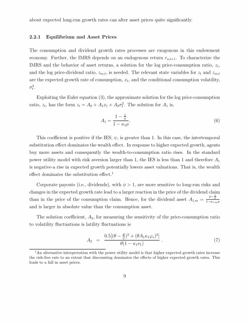
Exploiting the Euler equation (3), the approximate solution for the log price-consumption

ratio, zt, has the form zt = A0 + A1xt + A2σ2t . The solution for A1 is,

A1 =1 − 1

ψ

1 − κ1ρ. (6)

This coefficient is positive if the IES, ψ, is greater than 1. In this case, the intertemporal

substitution effect dominates the wealth effect. In response to higher expected growth, agents

buy more assets and consequently the wealth-to-consumption ratio rises. In the standard

power utility model with risk aversion larger than 1, the IES is less than 1 and therefore A1

is negative-a rise in expected growth potentially lowers asset valuations. That is, the wealth

effect dominates the substitution effect.1

Corporate payouts (i.e., dividends), with φ > 1, are more sensitive to long-run risks and

changes in the expected growth rate lead to a larger reaction in the price of the dividend claim

than in the price of the consumption claim. Hence, for the dividend asset A1,m =φ− 1

ψ

1−κ1,mρ

and is larger in absolute value than the consumption asset.

The solution coefficient, A2, for measuring the sensitivity of the price-consumption ratio

to volatility fluctuations is latility fluctuations is

A2 =0.5[(θ − θ

ψ)2 + (θA1κ1ϕe)

2]

θ(1 − κ1ν1). (7)

1An alternative interpretation with the power utility model is that higher expected growth rates increasethe risk-free rate to an extent that discounting dominates the effects of higher expected growth rates. Thisleads to a fall in asset prices.

9

An analogous coefficient for the market price-dividend ratio, A2,m, is provided in BY.

The expression for A2 provides two valuable insights. First, if the IES and risk aversion are

larger than 1, then θ and consequently A2 are negative. In this case, a rise in consumption

volatility lowers asset valuations and increases the risk premia on all assets. Second, an

increase in the permanence of volatility shocks — that is, an increase in ν1 — magnifies

the effects of volatility shocks on valuation ratios as investors perceive changes in economic

uncertainty as very long lasting.

2.2.2 Pricing of Short-Run, Long-Run, and Volatility Risks

Substituting the solutions for the price-consumption ratio, zt, into the expression for equilib-

rium return for ra,t+1 in equation (4), one can now characterize the solution for the IMRS that

can be used to value all assets. The log of the IMRS mt+1 can always be stated as the sum

of its conditional mean and its one-step-ahead innovation. The conditional mean is affine in

expected mean and conditional variance of consumption growth and can be expressed as,

Et(mt+1) = m0 −1

ψxt +

( 1ψ− γ)(γ − 1)

2

[

1 +

(

κ1ϕe1 − κ1ρ

)2]

σ2t . (8)

m0 is a constant determined by the preference and consumption dynamics parameters.

The innovation in the IMRS is very important for thinking about risk compensation (risk

premia) in various markets. Specifically, it is equal to

mt+1 − Et(mt+1) = −λm,ησtηt+1 − λm,eσtet+1 − λm,wσwwt+1, (9)

where λm,η, λm,e, and λm,w are the market prices for the short-run, long-run, and volatil-

ity risks, respectively. The market prices of systematic risks, including the compensation

for stochastic volatility risk in consumption, can be expressed in terms of the underlying

preferences parameters that govern the evolution of consumption growth:

λm,η = γ

λm,e = (γ −1

ψ)[ κ1ϕe1 − κ1ρ

]

(10)

10

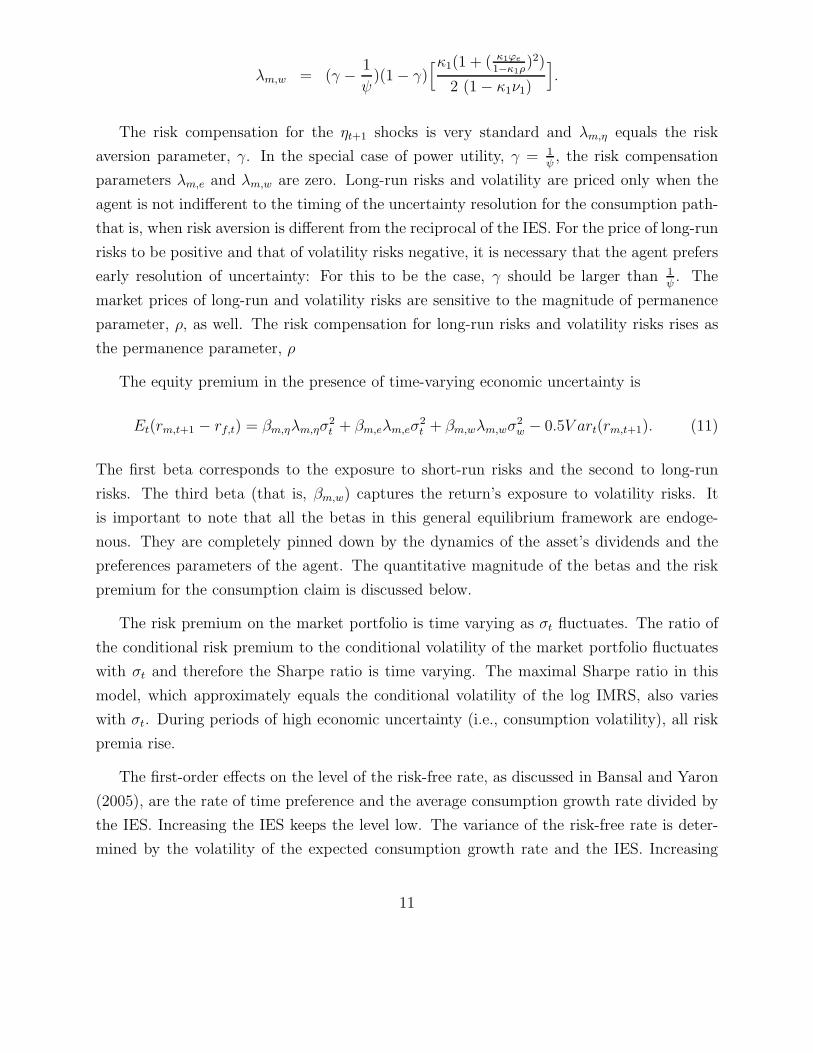
λm,w = (γ −1

ψ)(1 − γ)

[κ1(1 + ( κ1ϕe1−κ1ρ

)2)

2 (1 − κ1ν1)

]

.

The risk compensation for the ηt+1 shocks is very standard and λm,η equals the risk

aversion parameter, γ. In the special case of power utility, γ = 1ψ, the risk compensation

parameters λm,e and λm,w are zero. Long-run risks and volatility are priced only when the

agent is not indifferent to the timing of the uncertainty resolution for the consumption path-

that is, when risk aversion is different from the reciprocal of the IES. For the price of long-run

risks to be positive and that of volatility risks negative, it is necessary that the agent prefers

early resolution of uncertainty: For this to be the case, γ should be larger than 1ψ. The

market prices of long-run and volatility risks are sensitive to the magnitude of permanence

parameter, ρ, as well. The risk compensation for long-run risks and volatility risks rises as

the permanence parameter, ρ

The equity premium in the presence of time-varying economic uncertainty is

Et(rm,t+1 − rf,t) = βm,ηλm,ησ2t + βm,eλm,eσ

2t + βm,wλm,wσ

2w − 0.5V art(rm,t+1). (11)

The first beta corresponds to the exposure to short-run risks and the second to long-run

risks. The third beta (that is, βm,w) captures the return’s exposure to volatility risks. It

is important to note that all the betas in this general equilibrium framework are endoge-

nous. They are completely pinned down by the dynamics of the asset’s dividends and the

preferences parameters of the agent. The quantitative magnitude of the betas and the risk

premium for the consumption claim is discussed below.

The risk premium on the market portfolio is time varying as σt fluctuates. The ratio of

the conditional risk premium to the conditional volatility of the market portfolio fluctuates

with σt and therefore the Sharpe ratio is time varying. The maximal Sharpe ratio in this

model, which approximately equals the conditional volatility of the log IMRS, also varies

with σt. During periods of high economic uncertainty (i.e., consumption volatility), all risk

premia rise.

The first-order effects on the level of the risk-free rate, as discussed in Bansal and Yaron

(2005), are the rate of time preference and the average consumption growth rate divided by

the IES. Increasing the IES keeps the level low. The variance of the risk-free rate is deter-

mined by the volatility of the expected consumption growth rate and the IES. Increasing

11

the IES lowers the volatility of the risk-free rate. In addition, incorporating economic uncer-

tainty leads to an interesting channel for interpreting fluctuations in the real risk-free rate.

In addition, this has serious implications for the measurement of the IES in the data, which

heavily relies on the link between the risk-free rate and expected consumption growth. In

the presence of varying volatility, the estimates of IES based on the projections considered

in Hall (1988) and Campbell (1999) are seriously biased downward.

Hansen, Heaton, and Li (2005) also consider a long-run risks model specification where

the IES is pinned at 1. This specific case affords considerable simplicity, as the wealth-to-

consumption ratio is constant. To solve the model at values of the IES that differ from 1, the

authors provide approximations around the case where IES is 1. Bansal, Kiku, and Yaron

(2006) provide an alternative approximate solution that relies on equation (4); they show

how to derive the return ra,t along with the endogenous approximating constants κ1 and κ0

for any configuration of preferences parameters.

3 Data and Model Implications

3.1 Data and Growth Rate Dynamics

BY calibrate the model described in (5) at the monthly frequency. From this monthly model

they derive time-aggregated annual growth rates of consumption and dividends to match key

aspects of annual aggregate consumption and dividends data. For consumption, Bureau of

Economic Analysis data on real per capita annual consumption growth of non-durables and

services for the period 1929-98 is used. Dividends and the value-weighted market return data

are taken from the Center for Research in Security Prices (CRSP). All nominal quantities

are deflated using the CPI.

The mean annual real per-capita consumption growth rate is 1.8 percent, and its standard

deviation is about 2.9 percent. Table 1, adapted from BY, shows that, in the data, con-

sumption growth has a large first-order autocorrelation coefficient and a small second-order

coefficient. The standard errors in the data for these autocorrelations are sizeable. An alter-

native way to view the long-horizon property of the consumption and dividend growth rates

is to use variance ratios, which are themselves determined by the autocorrelations (Cochrane,

1988). In the data, the variance ratios first rise significantly and at a horizon of about seven

12

years start to decline. The standard errors on these variance ratios, not surprisingly, are

quite substantial.

In terms of the specific parameters for the consumption dynamics, BY calibrate ρ at

0.979, which determines the persistence in the long-run component in growth rates. Their

choice of ϕe and σ ensures that the model matches the unconditional variance and the

autocorrelation function of annual consumption growth. The standard deviation of the

innovation in consumption equals 0.0078. This parameter configuration implies that the

predictable variation in monthly consumption growth is very small — the implied R2 is

only 4.4 percent. The exposure of the corporate sector to long-run risks is governed by

φ, and its magnitude is similar to that in Abel (1999). The standard deviation of the

monthly innovation in dividends, ϕdσ, is 0.0351. The parameters of the volatility process

are chosen to capture the persistence in consumption volatility. Based on the evidence of

slow decay in volatility shocks, BY calibrate ν1, the parameter governing the persistence of

conditional volatility, at 0.987. The shocks to the volatility process have very small volatility;

σw is calibrated at 0.23 × 10−5. At the calibrated parameters, the modeled consumption

and dividend growth rates very closely match the key consumption and dividends data

features reported in Table 1. Bansal, Gallant, and Tauchen (2007) provide simulation-based

estimation evidence that supports this configuration as well.

Table 2 presents the targeted asset market data for 1929-98. The equity risk premium

is 6.33 percent per annum, and the real risk-free rate is 0.9 percent. The annual market

return volatility is 19.42 percent, and that of the real risk-free rate is quite small, about 1

percent per annum. The volatility of the price-dividend ratio is quite high, and it is a very

persistent series. In addition to these data dimensions, BY also evaluate the ability of the

model to capture predictability of returns. Bansal, Khatchatrian, and Yaron (2005) show

that, consistent with the implications of the BY model, price-dividend ratios are negatively

correlated with consumption volatility at long leads and lags.

It is often argued that, in the data, consumption and dividend growth are close to being

i.i.d. BY show that their model of consumption and dividends is also consistent with the

observed data on consumption and dividends growth rates. However, although the financial

market data are hard to interpret from the perspective of the i.i.d. growth rate dynamics,

BY show that it is interpretable from the perspective of the growth rate dynamics that

incorporate long-run risks. Given these difficulties in discrimination across these two models,

Hansen and Sargent (2006) use features of the long-run model for developing economic models

13

where agents update their model beliefs in a manner that incorporates robustness against

model misspecification.

3.2 Preference Parameters

The preference parameters take account of economic considerations. The time preference

parameter, δ < 1, and the risk aversion parameter, γ, is either 7.5 or 10. Mehra and

Prescott (1985) argue that a reasonable upper bound for risk aversion is around 10. The IES

is set at 1.5: An IES value that is not less than 1 is important for the quantitative results.

There is considerable debate about the magnitude of the IES. Hansen and Singleton

(1982) and Attanasio and Weber (1989) estimate the IES to be well in excess of 1. More

recently, Guvenen (2001) and Vissing-Jorgensen and Attanasio (2003) also estimate the IES

over 1; they show that their estimates are close to that used in BY. However, Hall (1988) and

Campbell (1999) estimate the IES to be well below 1. BY argue that the low IES estimates

of Hall and Campbell are based on a model without time-varying volatility. They show that

ignoring the effects of time-varying consumption volatility leads to a serious downward bias

in the estimates of the IES. If the population value of the IES in the BY model is 1.5, then

the estimated value of the IES using Hall estimation methods will be less than 0.3. With

fluctuating consumption volatility, the projection of consumption growth on the level of the

risk-free rate does not equal the IES, leading to the downward bias. This suggests that Hall’s

and Campbell’s estimates may not be a robust guide for calibrating the IES.

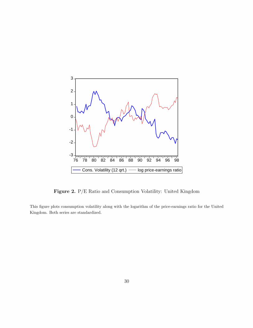
In addition to the above arguments, the empirical evidence in Bansal, Khatchatrian, and

Yaron (2005) shows that a rise in consumption volatility sharply lowers asset prices at long

leads and lags, and high current asset valuations forecast higher future corporate earnings

growth. Figures 1 through 4 use data from the United States, United Kingdom, Germany,

and Japan to evaluate the volatility channel. The asset valuation measure is the price-to-

earnings ratio, and the consumption volatility measure is constructed by averaging eight

lags of the absolute value of consumption residuals. It is evident from the figures that a

rise in consumption volatility lowers asset valuations for all countries under consideration;

this highlights the volatility channel and motivates the specification of an IES larger than 1.

In a two-country extension of the model, Bansal and Shaliastovich (2007) show that dollar

prices of foreign currency and forward premia co-move negatively with the consumption

volatility differential, whereas the ex ante currency returns have positive correlations with

14

it. This provides further empirical support for a magnitude of the IES. In terms of growth

rate predictability, Ang and Bekaert (2007) and Bansal, Khatchatrian, and Yaron (2005)

report a positive relation between asset valuations and expected earnings growth. These

data features, as discussed in the theory sections above, again require an IES larger than 1.

3.3 Asset Pricing Implications

To underscore the importance of two key aspects of the model, preferences and long-run

risks, first consider the genesis of the risk premium on ra,t+1 — the return on the asset that

delivers aggregate consumption as its dividends. The determination of risk premia for other

dividend claims follows the same logic.

Table 3 shows the market price of risk and the breakdown of the risk premium from

various risk sources. Column 1 considers the case of power utility where IES equals the

reciprocal of the risk aversion parameter. As discussed earlier, the prices of long-run and

volatility risks are zero. In the power utility case, the main risk is the short-run risk and the

risk premium on the consumption asset equals γσ2, which is 0.7 percent per annum.

Column 2 of Table 3 considers the case with an IES less than 1 (set at 0.5). For long-run

growth rate risks, the price of risk is positive; for volatility risks, the price of risk is negative,

as γ is larger than the reciprocal of the IES. However, the consumption asset’s beta for long-

run risks (beta with regard to the innovations in xt+1) is negative. This, as discussed earlier,

is because A1 is negative (see equation (6)), implying that a rise in expected growth lowers the

wealth-to-consumption ratio. Consequently, long-run risks in this case contribute a negative

risk premium of -1.96 percent per annum. The market price of volatility risks is negative and

small; however, the asset’s beta for this risk source is large and positive, reflecting the fact

that asset prices rise when economic uncertainty rises (see equation (7)). In all, when the

IES is less than 1, the risk premium on the consumption asset is negative, which is highly

counterintuitive, and highlights the implausibility of this parameter configuration.

Column 3 of Table 3 shows that when the IES is larger than 1, the price of long-run

growth risks rises. More importantly, the asset’s beta for long-run growth risks is positive

and that for volatility risks is negative. Both these risk sources contribute toward a positive

risk premium. The risk premium from long-run growth is 0.76 percent and that for the

short-run consumption shock is 0.73 percent. The overall risk premia for this consumption

15

asset is 1.52 percent. This evidence shows that an IES larger than 1 is required for the

long-run and volatility risks to carry a positive risk premium.

It is clear from Table 3 that the price of risk is highest for the long-run risks (see columns

2 and 3) and smallest for the volatility risks. A comparison of column 2 and 3 also shows that

raising the IES increases the prices of long-run and volatility risks in absolute value. The

magnitudes reported in Table 3 are with ρ = 0.979 — lowering this persistence parameter

also lowers the prices of long-run and volatility risks (in absolute value). Increasing the risk

aversion parameter increases the prices of all consumption risks. Hansen and Jagannathan

(1991) document the importance of the maximal Sharpe ratio, determined by the volatility

of the IMRS, in assessing asset pricing models. Incorporating long-run risks increases the

maximal Sharpe ratio in the model, which easily satisfies the non-parametric bounds of

Hansen and Jagannathan (1991).

The risk premium on the market portfolio (i.e., the dividend asset) is also affected by the

presence of long-run risks. To underscore their importance, assume that consumption and

dividend growth rates are i.i.d. This shuts off the long-run risks channel. The market risk

premium in this case is

Et(rm,t+1 − rf,t) = γcov(gt+1, gd,t+1) − 0.5V ar(gd,t+1), (12)

and market return volatility equals the dividend growth rate volatility. If shocks to consump-

tion and dividends are uncorrelated, then the geometric risk premium is negative and equals

−0.5V ar(gd,t+1). If the correlation between monthly consumption and dividend growth is

0.25, then the equity premium is 0.08 percent per annum, which is similar to the evidence

documented in Mehra and Prescott (1985) and Weil (1989).

BY show that their model, which incorporates long-run growth rate risks and fluctuating

economic uncertainty provides a very close match to the asset market data reported in Table

2. That is, the model can account for the low risk-free rate, high equity premium, high

asset price volatility, and low risk-free rate volatility. The BY model matches additional

data features, such as (i) predictability of returns at short and long horizons using dividend

yield as a predictive variable, (ii) time-varying and persistent market return volatility, (iii)

negative correlation between market return and volatility shocks, i.e., the volatility feedback

effect, and the (iv) negative relation between consumption volatility and asset prices at long

leads and lags. (Also see Bansal, Khatchatrian and Yaron, 2005.)

16

3.4 Cross-Sectional Implications

Table 4, shows that there are sizable differences in mean real returns across portfolios sorted

by book-to-market ratio, size, and momentum for quarterly data from 1967 to 2001. The size

and book-to-market sorts place firms into different deciles once per year, and the subsequent

return on these portfolios is used for empirical work. For momentum assets, CRSP-covered

New York Stock Exchange and American Stock and Options Exchange stocks are sorted on

the basis of their cumulative return over months t-12 through t -1. The loser portfolio (m1)

includes firms with the worst performance over the past year, and the winner portfolio (m10)

includes firms with the best performance. The data show that subsequent returns on these

portfolios have a large spread (i.e., m10 return - m1 return), about 4.62 percent per quarter:

This is the momentum spread puzzle. Similarly, the highest book-to-market firms (b10) earn

average real quarterly returns of 3.27 percent, whereas the lowest book-to-market (b1) firms

average 1.54 percent per quarter. The value spread (return on b10 - return on b1) is about

2 percent per quarter: This is the value spread puzzle. What explains these big differences

in mean returns across portfolios?

Bansal, Dittmar, and Lundblad (2002 and 2005) connect systematic risks to cash-flow

risks. They show that an asset’s risk measure (i.e., its beta) is determined by its cash-flow

properties. In particular, their paper shows that cross-sectional differences in asset betas

mostly reflect differences in systematic risks in cash flows. Hence, systematic risks in cash

flows ought to explain differences in mean returns across assets. They develop two ways

to measure the long-run risks in cash flows. First they model dividend and consumption

growth rates as a VAR and measure the discounted impulse response of the dividend growth

rates to consumption innovations. This is one measure of risks in cash flows. Their second

measure is based on stochastic cointegration, which is estimated by regressing the log level

of dividends for each portfolio on a time trend and the log level of consumption. Specifically,

consider the projection

dt = τ(0) + τ(1)t+ τ(2)ct + ζt,

where the projection coefficient, τ(2), measures the long-run consumption risk in the asset’s

dividends. The coefficient τ(2) will be different for different assets.

Bansal, Dittmar, and Lundblad (2002 and 2005) show that the exposure of dividend

growth rates to the long-run component in consumption has considerable cross-sectional

explanatory power. That is, dividend’s exposure to long-run consumption risks is an im-

17

portant explanatory variable in accounting for differences in mean returns across portfolios.

Portfolios with high mean returns also have higher dividend exposure to consumption risks.

The cointegration-based measure of risk, τ(2), also provides very valuable information about

mean returns on assets. The cross-sectional R2 from regressing the mean returns on the

dividend-based risk measures is well over 65 percent. In contrast, other approaches find it

quite hard to explain the differences in mean returns for the 30-asset menu used in Bansal,

Dittmar, and Lundblad (2005). The standard consumption betas (i.e., C-CAPM) and the

market-based CAPM asset betas have close to zero explanatory power. The R2 for the C-

CAPM is 2.7 percent, and that for the market CAPM is 6.5 percent, with an implausible

negative slope coefficient. The Fama and French three-factor empirical specification also gen-

erates point estimates with negative, and difficult to interpret, prices of risk for the market

and size factors; the cross-sectional R2 is about 36 percent. Compared with all these models,

the cash-flow risks model of Bansal, Dittmar, and Lundblad (2005) is able to capture a sig-

nificant portion of the differences in risk premia across assets. Hansen, Heaton, and Li (2005)

inquire about the robustness of the stochastic cointegration-based risk measures considered

in Bansal, Dittmar, and Lundblad (2002). They argue that the dividend-based consumption

betas-particularly, the cointegration-based risk measures-are imprecisely estimated in the

time series. Interestingly, across the different estimation procedures, the cash-flow beta risk

measures across portfolios line-up closely with the average returns across assets. That is, in

the cross-section of assets (as opposed to the time series), the price of risk associated with

the long-run risks measures is reliably significant.

Bansal, Dittmar, and Kiku (2007) derive new results that link this cointegration param-

eter to consumption betas by investment horizon and evaluate the ability of their model

to explain differences in mean returns for different horizons. They provide new evidence

regarding the robustness of the stochastic cointegration-based measures of permanent risks

in equity markets. Parker and Julliard (2005) evaluate whether long-run risks in aggre-

gate consumption can account for the cross-section of expected returns. Malloy, Moskowitz,

and Vissing-Jorgensen (2005) evaluate whether long-run risks in stockholders’ consumption

relative to aggregate consumption has greater ability to explain the cross-section of equity

returns, relative to aggregate consumption measures.

18

3.5 Term Structure and Currency Markets

Colacito and Croce (2006) consider a two-country version of the BY model. They show

that this model can account for the low correlation in consumption growth across coun-

tries but high correlation in marginal utilities across countries (high risk sharing despite a

low measured cross-country consumption correlation). This feature of international data is

highlighted in Brandt, Cochrane, and Santa-Clara (2006). The key idea that Colacito and

Croche pursue is that the long-run risks component is very similar across countries, but in

the short-run consumption growth can be very different. That is, countries share very similar

long-run prospects, but in the short-run they can look very different. This dimension, they

show, is sufficient to induce high correlation in marginal utilities across countries. It also

accounts for high real exchange volatility.

BY derive implications for the real term structure of interest rates for the long-run risks

model. More recent papers by Eraker (2006) and Piazzesi and Schneider (2005) also consider

the quantitative implications for the nominal term structure using the long-run risks model.

Bansal and Shaliastovich (2007) show that the BY model can simultaneously account for the

upward-sloping terms structure, the violations of the expectations hypothesis in the bond

markets, the violations in the foreign currency markets, and the equity returns. This evidence

indicates that the long-run risks model provides a solid baseline model for understanding

financial markets. With simple modifications the model can be used to analyze the impact

of changing short-term interest rates on financial markets; that is, it can help in designing

policy.

4 Conclusion

The work of Bansal and Lundblad (2002), Bansal and Yaron (2004), Bansal, Dittmar, and

Lundblad (2005) shows that the long-run risks model can help interpret several features

of financial markets. These papers argue that investors care about the long-run growth

prospects and the uncertainty (time-varying consumption volatility) surrounding the growth

rate. Risks associated with changing long-run growth prospects and varying economic un-

certainty drive the level of equity returns, asset price volatility, risk premia across assets,

and predictability of returns in financial markets.

19

Recent papers indicate that the channel in this model can account for nominal yield curve

features, such as the violation the expectations hypothesis and the average upward-sloping

nominal yield curve. Evidence presented in Colacito and Croce (2006) and Bansal and

Shaliastovich (2007) shows that the model also accounts for key aspects of foreign exchange

markets.

Growing evidence suggests that the long-run risks model can explain a rich array of

financial market facts. This suggests that the model can be used to analyze the impact of

economic policy on financial markets.

20

References

Abel, Andrew B. 1999. “Risk Premia and Term Premia in General Equilibrium.” Journal of

Monetary Economics 43:3–33.

Ang, Andrew and Geert Bekaert. 2005. “Stock Return Predictability: Is It There?” Working

paper.

Attanasio, P. Orazio and Guglielmo Weber. 1989. “Intertemporal Substitution, Risk Aversion

and the Euler Equation for Consumption.” Economic Journal 99:59–73.

Bansal, Ravi and Amir Yaron. 2004. “Risks for the Long Run: A Potential Resolution of

Asset Pricing Puzzles.” Journal of Finance 59(4):1481–1509.

Bansal, Ravi and Amir Yaron. 2005. “The Asset Pricing-Macro Nexus and Return-Cash

Flow Predictability.” Working paper.

Bansal, Ravi and Christian Lundblad. 2002. “Market Efficiency, Asset Returns, and the Size

of the Risk Premium in Global Equity Markets.” Journal of Econometrics 109:195–237.

Bansal, Ravi, Dana Kiku and Amir Yaron. 2006. “Risks for the Long Run: Estimation and

Inference.” Working paper .

Bansal, Ravi and Ivan Shaliastovich. 2007. “Risk and Return in Bond, Currency and Equity

Markets: A Unified Approach.” Working paper.

Bansal, Ravi, R. Dittmar and C. Lundblad. 2002. “Interpreting Risk Premia Across Size,

Value and Industry Portfolios.” Working Paper.

Bansal, Ravi, R. Dittmar and C. Lundblad. 2005. “Consumption, Dividends, and the Cross-

section of Equity Returns.” Journal of Finance 60:1639–1672.

Bansal, Ravi, Robert Dittmar and Dana Kiku. 2007. “Cointegration and Consumption Risks

in Asset Returns.” Forthcoming in Review of Financial Studies.

Bansal, Ravi, Ronald Gallant and George Tauchen. 2005. “Rational Pessimism, Rational

Exuberance, and Markets For Macro Risks.” Working paper, Duke University.

Bansal, Ravi, Varoujan Khatchatrian and Amir Yaron. 2005. “Interpretable Asset Markets.”

European Economic Review 49:531–560.

21

Brandt, Michael, J. Cochrane and P. Santa-Clara. 2005. “International Risk Sharing is Better

Than You Think (or Exchange Rates are Much Too Smooth).” Forthcoming Journal of

Monetary Economics .

Campbell, John and Robert Shiller. 1988. “The Dividend-Price Ratio and Expectations of

Future Dividends and Discount Factors.” The Review of Financial Studies 1(3):195–228.

Campbell, John Y. 1999. Asset Prices, Consumption and the Business Cycle. In Handbook

of Macroeconomics, ed. John B. Taylor and Michael Woodford. Vol. 1 Elsevier Science,

North Holland, Amsterdam.

Cecchetti, Stephen G., Pok-Sang Lam and Nelson C. Mark. 1993. “The Equity Premium and

the Risk Free Rate: Matching the Moments.” Journal of Monetary Economics 31:21–46.

Chen, Hui. 2006. “Macroeconomic Conditions and the Puzzles of Credit Spreads and Capital

Structure.” Working paper.

Chen, Long, P. Collin-Dufresne and R. S. Goldstein. 2006. “On the Relation Between the

Credit Spread Puzzle and the Equity Premium Puzzle.” Working paper.

Cochrane, John H. 1988. “How Big is the Random Walk in GNP?” Journal of Political

Economy 96:893–920.

Colacito, Riccardo and Maiano M. Croce. 2006. “Risks for the Long Run and the Real

Exchange Rate.” Working paper .

Epstein, L.G and S. Zin. 1989. “Substitution, Risk Aversion and the Temporal Behavior of

Consumption and Asset Returns: A Theoretical Framework.” Econometrica 57:937–969.

Eraker, Bjørn. 2006. “Affine General Equilibrium Models.” Working paper .

Fama, E.F. 1984. “Forward and Spot Exchange Rates.” Journal of Monetary Economics

14:319–338.

Fama, E.F. and R. Bliss. 1987. “The Information in Long-Maturity Forward Rates.” Amer-

ican Economic Review 77:680–692.

Guvenen, Fatih. 2001. “Mismeasurement of the Elasticity of Intertemporal Substitution:

The Role of Limited Stock Market Participation.” Unpublished manuscript, University

of Rochester.

22

Hall, Robert E. 1988. “Intertemporal Substitution in Consumption.” Journal of Political

Economy 96:339–357.

Hansen, L. P and Ravi Jagannathan. 1991. “Implications of Security Market Data for Models

of Dynamic Economies.” Journal of Political Economy 99:225–262.

Hansen, Lars P. and Kenneth Singleton. 1982. “Generalized Instrumental Variables Estima-

tion of Nonlinear Rational Expectations Model.” Econometrica 50:1269–1286.

Hansen, Lars Peter, John C. Heaton and Nan Li. 2005. “Consumption Strikes Back?: Mea-

suring Long-Run Risk.” Working paper.

Hansen, Lars and Thomas Sargent. 2006. “Fragile Beliefs and the Price of Model Uncer-

tainty.” Working paper .

Kiku, Dana. 2006. “Is the Value Premium a Puzzle?” Working paper .

Lettau, Martin, Sydney Ludvigson and Jessica Wachter. 2006. “The Declining Equity Pre-

mium: What Role Does Macroeconomic Risk Play?” Forthcoming in Review of Finan-

cial Studies.

Lochstoer, Lars and Georg Kaltenbrunner. 2006. “Long-Run Risk through Consumption

Smoothing.” Working paper.

Lucas, Robert. 1978. “Asset Prices in an Exchange Economy.” Econometrica 46:1429–1446.

Malloy, Christopher J., Tobias J. Moskowitz and Annette Vissing-Jørgensen. 2005. “Long-

Run Stockholder Consumption Risk and Asset Returns.” Working paper.

Mehra, Rajnish and Edward C. Prescott. 1985. “The Equity Premium: A Puzzle.” Journal

of Monetary Economics 15:145–161.

Parker, Jonathan and Christian Julliard. 2005. “Consumption Risk and the Cross-Section

of Asset Returns.” Journal of Political Economy 113:185–222.

Piazzesi, Monika and Martin Schneider. 2005. “Equilibrium Yield Curves.”. NBER Working

Paper 12609.

Shiller, Robert J. 1981. “Do Stock Prices Move Too Much to Be Justified by Subsequent

Changes in Dividends?” American Economic Review 71:421–436.

23

Vissing-Jorgensen, Annette and P. Orazio Attanasio. 2003. “Stock Market Participation,

Intertemporal Substitution and Risk Aversion.” American Economic Review (Papers

and Proceedings) 93:383–391.

Weil, Philippe. 1989. “The Equity Premium Puzzle and the Risk Free Rate Puzzle.” Journal

of Monetary Economics 24:401–421.

24

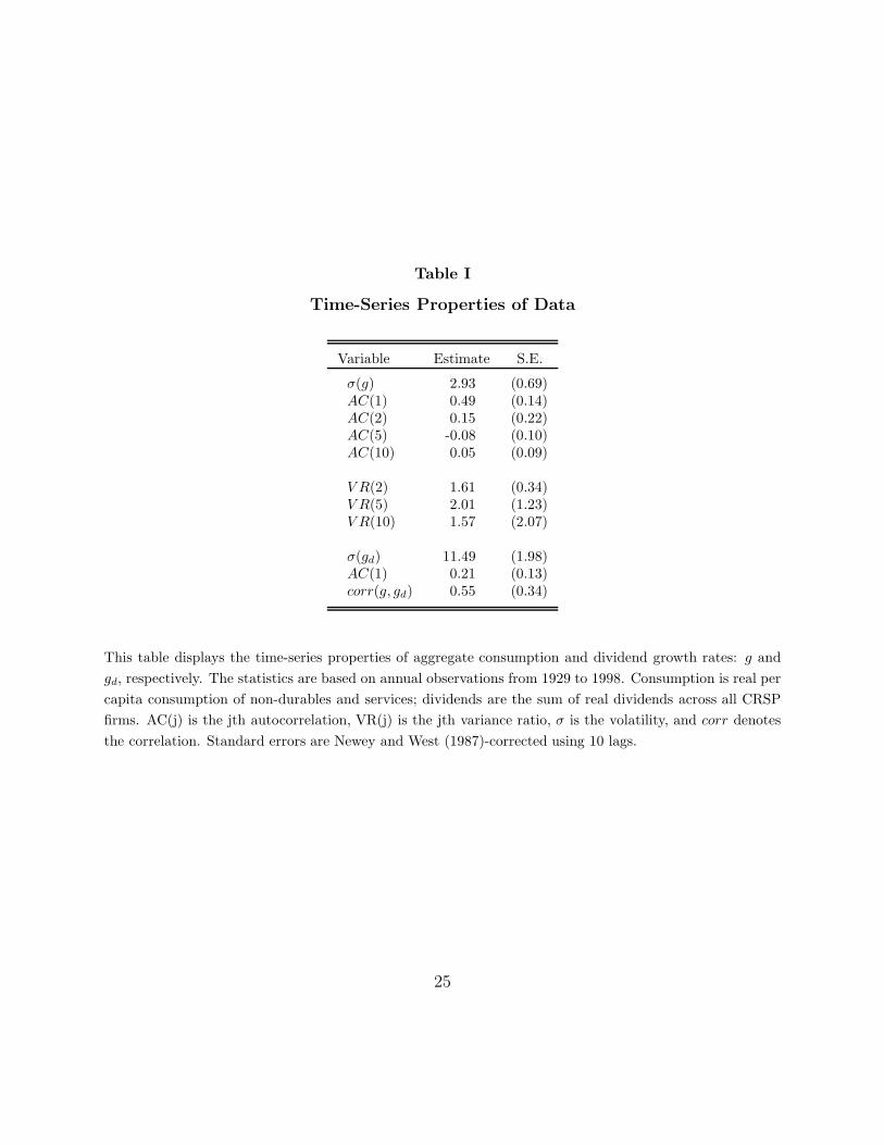
Table I

Time-Series Properties of Data

Variable Estimate S.E.

σ(g) 2.93 (0.69)AC(1) 0.49 (0.14)AC(2) 0.15 (0.22)AC(5) -0.08 (0.10)AC(10) 0.05 (0.09)

V R(2) 1.61 (0.34)V R(5) 2.01 (1.23)V R(10) 1.57 (2.07)

σ(gd) 11.49 (1.98)AC(1) 0.21 (0.13)corr(g, gd) 0.55 (0.34)

This table displays the time-series properties of aggregate consumption and dividend growth rates: g and

gd, respectively. The statistics are based on annual observations from 1929 to 1998. Consumption is real per

capita consumption of non-durables and services; dividends are the sum of real dividends across all CRSP

firms. AC(j) is the jth autocorrelation, VR(j) is the jth variance ratio, σ is the volatility, and corr denotes

the correlation. Standard errors are Newey and West (1987)-corrected using 10 lags.

25

Table II

Asset Market Data

Variable Estimate S.E.

Returns

E(rm − rf ) 6.33 (2.15)E(rf ) 0.86 (0.42)σ(rm) 19.42 (3.07)σ(rf ) 0.97 (0.28)

Price-Dividend Ratio

E(exp(p− d)) 26.56 (2.53)σ(p− d) 0.29 (0.04)AC1(p− d) 0.81 (0.09)AC2(p− d) 0.64 (0.15)

This table presents descriptive statistics of asset market data. The moments are calculated using annual

observations from 1929 through 1998. E(rm−rf ) and E(rf ) are, respectively, the annualized equity premium

and mean risk-free-rate; σ(rm), σ(rf ), and σ(p − d), respectively, the annualized volatilities of the market

return, risk-free rate, and log price-dividend ratio; AC1 and AC2 denote the first and second autocorrelations.

Standard errors are Newey and West (1987)-corrected using 10 lags.

26

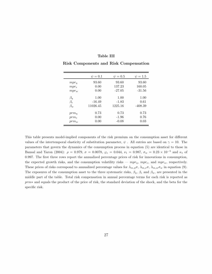
Table III

Risk Components and Risk Compensation

ψ = 0.1 ψ = 0.5 ψ = 1.5

mprη 93.60 93.60 93.60mpre 0.00 137.23 160.05mprw 0.00 -27.05 -31.56

βη 1.00 1.00 1.00βe -16.49 -1.83 0.61βw 11026.45 1225.16 -408.39

prmη 0.73 0.73 0.73prme 0.00 -1.96 0.76prmw 0.00 -0.08 0.03

This table presents model-implied components of the risk premium on the consumption asset for different

values of the intertemporal elasticity of substitution parameter, ψ . All entries are based on γ = 10. The

parameters that govern the dynamics of the consumption process in equation (5) are identical to those in

Bansal and Yaron (2004): ρ = 0.979, σ = 0.0078, ϕe = 0.044, ν1 = 0.987, σw = 0.23 × 10−5 and κ1 of

0.997. The first three rows report the annualized percentage prices of risk for innovations in consumption,

the expected growth risks, and the consumption volatility risks — mprη, mpre, and mprw, respectively.

These prices of risks correspond to annualized percentage values for λm,ησ, λm,eσ, λm,wσw in equation (9).

The exposures of the consumption asset to the three systematic risks, βη, βe and βw, are presented in the

middle part of the table. Total risk compensation in annual percentage terms for each risk is reported as

prm∗ and equals the product of the price of risk, the standard deviation of the shock, and the beta for the

specific risk.

27

Table IV

Portfolio returns

Mean Std. Dev Mean Std. Dev Mean Std. Dev

S1 0.0230 0.1370 B1 0.0154 0.1058 M1 -0.0104 0.1541S2 0.0231 0.1265 B2 0.0199 0.0956 M2 0.0070 0.1192S3 0.0233 0.1200 B3 0.0211 0.0921 M3 0.0122 0.1089S4 0.0233 0.1174 B4 0.0218 0.0915 M4 0.0197 0.0943S5 0.0242 0.1112 B5 0.0200 0.0798 M5 0.0135 0.0869S6 0.0207 0.1050 B6 0.0234 0.0813 M6 0.0160 0.0876S7 0.0224 0.1041 B7 0.0237 0.0839 M7 0.0200 0.0886S8 0.0219 0.1001 B8 0.0259 0.0837 M8 0.0237 0.0825S9 0.0207 0.0913 B9 0.0273 0.0892 M9 0.0283 0.0931S10 0.0181 0.0827 B10 0.0327 0.1034 M10 0.0358 0.1139

This table presents descriptive statistics for the returns on the 30 characteristic-sorted decile portfolios.

Value-weighted returns are presented for portfolios formed on momentum (M), market capitalization (S),

and book-to-market ratio (B). M1 represents the lowest momentum (loser) decile, S1 the lowest size (small

firms) decile, and B1 the lowest book-to-market decile. Data are converted to real values using the PCE

deflator. The data are sampled at the quarterly frequency and cover 1967:Q1-2001:Q4.

28

-3

-2

-1

0

1

2

3

55 60 65 70 75 80 85 90 95

Cons. Volatility (12 qrt.) log price-earnings ratio

Figure 1. P/E Ratio and Consumption Volatility: United States

This figure plots consumption volatility along with the logarithm of the price-earnings ratio for the United

States. Both series are standardized.

29

-3

-2

-1

0

1

2

3

76 78 80 82 84 86 88 90 92 94 96 98

Cons. Volatility (12 qrt.) log price-earnings ratio

Figure 2. P/E Ratio and Consumption Volatility: United Kingdom

This figure plots consumption volatility along with the logarithm of the price-earnings ratio for the United

Kingdom. Both series are standardized.

30

-3

-2

-1

0

1

2

3

76 78 80 82 84 86 88 90 92 94 96 98

Cons. Volatility (12 qrt.) log price-earnings ratio

Figure 3. P/E Ratio and Consumption Volatility: Germany

This figure plots consumption volatility along with the logarithm of the price-earnings ratio for Germany.

Both series are standardized.

31

-2

-1

0

1

2

3

76 78 80 82 84 86 88 90 92 94 96 98

Cons. Volatility (12 qrt.) log price-earnings ratio

Figure 4. P/E Ratio and Consumption Volatility: Japan

This figure plots consumption volatility along with the logarithm of the price-earnings ratio for Japan. Both

series are standardized.

32