NBER WORKING PAPER SERIES

INCOME AND DEMOCRACY

Daron AcemogluSimon Johnson

James A. RobinsonPierre Yared

Working Paper 11205http://www.nber.org/papers/w11205

NATIONAL BUREAU OF ECONOMIC RESEARCH1050 Massachusetts Avenue

Cambridge, MA 02138March 2005

We thank David Autor, Robert Barro, Jason Seawright, Sebastián Mazzuca, and seminar participantsat the Banco de la República de Colombia, Boston University, the Canadian Institute for Advanced Research,the CEPR annual conference on transition economics in Hanoi, MIT, and Harvard for comments. The viewsexpressed herein are those of the author(s) and do not necessarily reflect the views of the National Bureauof Economic Research.

© 2005 by Daron Acemoglu, Simon Johnson, James A. Robinson, and Pierre Yared. All rights reserved.Short sections of text, not to exceed two paragraphs, may be quoted without explicit permission providedthat full credit, including © notice, is given to the source.

Income and DemocracyDaron Acemoglu, Simon Johnson, James A. Robinson, and Pierre YaredNBER Working Paper No. 11205March 2005JEL No. P16, O10

ABSTRACT

We revisit one of the central empirical findings of the political economy literature that higher income

per capita causes democracy. Existing studies establish a strong cross-country correlation between

income and democracy, but do not typically control for factors that simultaneously affect both

variables. We show that controlling for such factors by including country fixed effects removes the

statistical association between income per capita and various measures of democracy. We also

present instrumental-variables using two different strategies. These estimates also show no causal

effect of income on democracy. Furthermore, we reconcile the positive cross-country correlation

between income and democracy with the absence of a causal effect of income on democracy by

showing that the long-run evolution of income and democracy is related to historical factors.

Consistent with this, the positive correlation between income and democracy disappears, even

without fixed effects, when we control for the historical determinants of economic and political

development in a sample of former European colonies.

Daron AcemogluDepartment of EconomicsMIT, E52-380B50 Memorial DriveCambridge, MA 02142-1347and NBER daron@mit.edu

Simon JohnsonSloan School of ManagementMIT, 50 Memorial DriveCambridge, MA 02139 and NBERsjohnson@mit.edu

James A. RobinsonDepartment of GovernmentHarvard University1875 Cambridge StreetCambridge, MA 02138jrobinson@gov.harvard.edu

Pierre YaredDepartment of EconomicsMIT50 Memorial DriveCambridge, MA 02142-1347yared@mit.edu

1 Introduction

One of the most notable empirical regularities in political economy is the relationship

between income per capita and democracy. Today all OECD countries are democratic,

while many of the nondemocracies are in the poor parts of the world, for example sub-

Saharan Africa and Southeast Asia. This positive relationship is not only confined to a

cross-country comparison. Most countries were nondemocratic before the modern growth

process took off at the beginning of the 19th century. Democratization came together

with growth. Barro (1999, S160), for example, summarizes the findings from his detailed

study as: “increases in various measures of the standard of living forecast a gradual rise

in democracy. In contrast, democracies that arise without prior economic development ...

tend not to last.”1

This statistical association between income and democracy is the cornerstone of the

influential modernization theory, which sees a direct causal link between economic growth

and democracy. According to this theory, economic growth engenders “a culture of democ-

racy” and provides the foundations for democratic political institutions. This thesis is

clearly articulated in Lipset (1959), who argued that “only in a wealthy society in which

relatively few citizens lived in real poverty could a situation exist in which the mass of the

population could intelligently participate in politics and could develop the self-restraint

necessary to avoid succumbing to the appeals of irresponsible demagogues” (p. 75). It

is also reproduced in all the major works on democracy (e.g., Dahl, 1971, Huntington,

1991).

In this paper, we revisit the relationship between income per capita and democracy.

Our starting point is that existing work, based on cross-country relationships, does not

establish causation. First, there is the issue of reverse causality; perhaps democracy

causes income rather than the other way round. Second, and more important, there is

the potential for omitted variable bias. Some other factor may determine both the nature

of the political regime and the potential for economic growth.

We utilize two strategies to investigate the causal effect of income on democracy. Our

first strategy is to control for country-specific factors affecting both income and democ-

racy by including country fixed effects. While fixed effect regressions are not a panacea

against omitted variable biases,2 they are well-suited to the investigation of the relation-

1Also see, among others, Lipset (1959), Londregan and Poole (1996), Przeworski and Limongi (1997),Barro (1997), Przeworski, Alvarez, Cheibub, and Limongi (2000), and Papaioannou and Siourounis(2004).

2Fixed effects would not help inference if there are time-varying omitted factors affecting the dependentvariable and correlated with the right-hand side variables (see the discussion below). They may also make

1

ship between income and democracy. Major sources of potential bias in a regression of

democracy on income per capita are country-specific, historical factors influencing both

political and economic development. If these omitted characteristics are, to a first approx-

imation, time-invariant, the inclusion of fixed effects will remove them and this source of

bias. Consider, for example, the comparison of the United States and Colombia. The

United States is both richer and more democratic, so a simple cross-country comparison,

as well as the existing empirical strategies in the literature which do not control for fixed

effects, would suggest that there is a relationship between democracy and income. The

idea of fixed effects is to move beyond this comparison and investigate the “within-country

variation”; i.e., whether as Colombia becomes relatively richer, it also tends to become

more democratic relative to the United States. In addition to improving inference on

the causal effect of income on democracy, this approach is also more closely related to

modernization theory as articulated by Lipset (1959), which claims that countries should

become more democratic as they become richer, not simply that rich countries should be

more democratic.

Our main finding from this strategy is that once fixed effects are introduced, the

positive relationship between income per capita and various measures of democracy dis-

appears. Figures 1 and 2 show this diagrammatically by plotting changes in our two

measures of democracy, the Freedom House and Polity scores (see below for data details),

for each country between 1970 and 1995 against the change in GDP per capita over the

same period. There appears to be no relationship between changes in income per capita

and democracy.

This basic finding holds with various indicators for democracy, with different econo-

metric specifications and estimation techniques, in different subsamples, and is robust to

the inclusion of additional covariates. Moreover, these results are not driven by large

standard errors. In many cases, two-standard error bands include only very small effects

of income on democracy, and often exclude the OLS estimates. These results therefore

shed considerable doubt on the claim that there is a strong causal effect of income on

democracy.3

While the fixed effects estimation is useful in removing the influence of long-run deter-

problems of measurement error worse because they remove a significant portion of the variation in theright-hand side variables. Consequently, fixed effects are certainly no substitute for using an instrumental-variables approach with a valid instrument.

3It remains true that over time there is a general tendency towards greater incomes and greaterdemocracy across the world. In our regressions, time effects capture these general (world-level) tendencies.Our estimates suggest that these world-level movements in democracy are unlikely to be driven by thecausal effect of income on democracy.

2

minants of both democracy and income, it does not necessarily estimate the causal effect

of income on democracy. An instrumental-variables (IV) strategy with a valid instrument

would be a superior approach, but it is difficult to find valid instruments for income that

could not affect democracy through other channels.4 Our second strategy is to use IV re-

gressions. We experiment with two potential instruments. The first is to use past savings

rates, while the second is to use changes in the incomes of trading partners. The argument

for the first instrument is that variations in past savings rates affect income per capita,

but should have no direct effect on democracy. The second instrument, which we believe

is of independent interest, creates a matrix of trade shares, and constructs predicted in-

come for each country using a trade-share-weighted average income of other countries.

We show that this predicted income has considerable explanatory power for income per

capita, and argue that it should have no direct effect on democracy. Both IV strategies

confirm our basic findings and show no evidence of a causal effect of income on democ-

racy. We recognize that neither instrument is perfect, since there are some reasonable

scenarios in which our exclusion restrictions could be violated (e.g., saving rates might

be correlated with future anticipated regime changes; or democracy scores of a country’s

trading partners, which are correlated with their income levels, might have a direct effect

on its democracy). To alleviate concerns about the validity of the instruments, we show

that the most likely sources of correlation between our instruments and the error term in

the second stage are not present.

These results naturally raise the following important question: what is the source of

the cross-sectional correlation between income and democracy? Why are rich countries

democratic today? One possible explanation is that there is a causal effect of income on

democracy, but it works at much longer horizons than the existing literature posited, that

is, over 50 or even 100 years rather than 10 or 20 years. Another hypothesis, suggested by

approaches that emphasize the importance of historical factors in long-run development,5

is that the cross-sectional relationship reflects the persistent influence of these historical

factors. Put differently, events during certain crucial junctures impact the economic and

political “development path” of a society, leading to persistent, though not permanent,

influences on economic and political outcomes. Both of these hypotheses suggest that the

within-correlation between income and democracy should be stronger when we look at

4A recent creative attempt is by Miguel, Satyanath and Sergenti (2004), who use the weather conditionsas an instrument for income in Africa for investigating the impact of income on civil wars. Unfortunately,weather conditions are only a good instrument for relatively short-run changes in income, thus notnecessarily ideal to study the relationship between income and democracy.

5See, among others, North and Thomas (1973), North (1981), Jones (1981), Engerman and Sokoloff(1997), Acemoglu, Johnson and Robinson (2001, 2002).

3

longer horizons.

We investigate this possibility by looking at the relationship between income and

democracy over the past 160 years, and over the past 500 years. We find little evidence

for an effect of income on democracy in samples that span 100 or 160 years. In contrast,

over the past 500 years there seems to be a very strong correlation. Our interpretation

is that this pattern is consistent with the second hypothesis, because the 500 years in

question spans the period of divergence of national development paths (e.g., the emergence

of constitutional monarchies, the rise of the modern nation state, industrialization, and

the colonial experience).

In addition, we also provide direct evidence consistent with the second hypothesis by

looking at the sample of former European colonies. This sample is useful since it enables

us to exploit the quasi-natural experiment provided by the colonization of many diverse

societies by European powers after 1492, where differences in the colonization experience

led to significant divergence in the economic and political development paths of these soci-

eties (see, e.g., Acemoglu, Johnson and Robinson, 2001, 2002, and Engerman and Sokoloff,

1997). We document that in this sample, the fixed effects in the democracy regressions

are closely linked to the potential determinants of European colonization strategy (in par-

ticular, the density of the indigenous population at the time of colonization and potential

mortality rates of European settlers), date of independence and measures of institutions

in the early independence era. The positive correlation between income and democracy

disappears, even without fixed effects, when we control for these historical determinants.

This evidence further supports the second hypothesis.

Finally, we document that there are some income-related determinants of democracy

in the postwar sample. In particular, contrary to the implications of modernization theory,

we find that economic crises lead to democracy. We show that this result is driven entirely

by the fact that dictatorships are more likely to collapse in the face of economic crises

than democracies are likely to revert back to dictatorship.6

The paper proceeds as follows. In Section 2 we describe the data. In Section 3 we

discuss our econometric approach and present the basic results. Section 4 presents our IV

results. Section 5 discusses potential interpretations for these results. Motivated by these

interpretations, Section 6 investigates the longer-run relationship between income and

democracy, and Section 7 looks at the historical determinants of economic and political

6In passing, we also show that income per capita does not appear to have a causal effect when we lookseparately at transitions to and from democracy, contrary to the findings in Przeworski et al. (2000).Since we do not have space in this paper, we leave a more detailed investigation of transitions to futurework.

4

development in the sample of former European colonies. Section 8 looks at the effect of

crises on democracy. Section 9 concludes. The Appendix contains some additional results

and further information on the construction of the instruments used in Section 4.

2 Data and Descriptive Statistics

We follow much of the existing research in this area in adopting a Schumpeterian definition

based on a number of institutional conditions.7 Our first and main measure of democracy

is the Freedom House Political Rights Index. A country receives the highest score if

political rights come closest to the ideals suggested by a checklist of questions, beginning

with whether there are free and fair elections, whether those who are elected rule, whether

there are competitive parties or other political groupings, whether the opposition plays an

important role and has actual power, and whether minority groups have reasonable self-

government or can participate in the government through informal consensus.8 Following

Barro (1999), we supplement this index with the related variable from Bollen (1990, 2001)

for 1950, 1955, 1960, and 1965. As in Barro (1999), we transform both indices so that

they lie between 0 and 1, with 1 corresponding to the most democratic set of institutions.

The Freedom House index, even when augmented with Bollen’s data, only enables us

to look at the postwar era. The Polity IV dataset, on the other hand, provides informa-

tion for all countries since independence starting in 1800. Both for pre-1950 events and

as a check on our main measure, we also look at the other widely-used measure of democ-

racy, the composite Polity index, which is the difference between Polity’s Democracy and

Autocracy indices (see Marshall and Jaggers, 2004). The Polity Democracy Index ranges

from 0 to 10 and is derived from coding the competitiveness of political participation, the

openness and competitiveness of executive recruitment and constraints on the chief exec-

utive. The Polity Autocracy Index also ranges from 0 to 10 and is constructed in a similar

way to the democracy score based on scoring countries according to competitiveness of

political participation, the regulation of participation, the openness and competitiveness

of executive recruitment and constraints on the chief executive. To facilitate compari-

7Schumpeter (1950, p. 250) argued that democracy was: “the institutional arrangement for arrivingat political decisions in which individuals acquire the power to decide by means of a competitive strugglefor the people’s vote.”

8The main checklist includes 3 questions on the electoral process, 4 questions on the extent of politicalpluralism and participation, and 3 questions on the functioning of government. For each checklist question,0 to 4 points are added, depending on the comparative rights and liberties present (0 represents the least,4 represents the most) and these scores are combined to form the index. See Freedom House (2004),http://www.freedomhouse.org/research/freeworld/2003/methodology.htm

5

son with the Freedom House score, we also normalize the composite Polity index to lie

between 0 and 1.

Using the Freedom House and the Polity data, we construct five-yearly, ten-yearly,

and annual panels. For the five-year panels, we take the observation every fifth year.

We prefer this procedure to averaging the five-yearly data, since averaging introduces

additional serial correlation, making inference and estimation more difficult (see footnote

12). For the ten-yearly panels, we take the observation every tenth year for similar reasons.

For the Freedom House data which begins in 1972, we follow Barro (1999) and assign the

1972 score to 1970 for the purpose of the five-year and ten-year regressions.

The GDP per capita (in PPP) and savings rate data for the postwar period are from

Heston, Summers, and Atten (2002), and GDP per capita (in constant 1990 dollars) for the

longer sample are from Maddison (2003). The trade-weighted world income instrument is

built using data from International Monetary Fund Direction of Trade Statistics (2005).

Other variables we use in the analysis are discussed later (see also Appendix Table A1 for

detailed data definitions and sources).

Table 1 contains descriptive statistics for the key variables both for the whole world

and for former European colonies, the sample we focus on for some of the historical

regressions. It shows that there is significant variation in all the variables for both the

entire sample and the former colonies sample. Countries in the former colonies sample are

somewhat less democratic and substantially (about 30 percent) poorer than the average

country in the whole sample.

3 Main Results

3.1 Basic Specifications and Interpretation

Our basic regression model is:

dit = αdit−1 + γyit−1 + x0it−1β + µt + δi + uit, (1)

where dit is the democracy score of country i in period t. The lagged value of this variable

on the right hand side is included to capture persistence in democracy and also potentially

mean-reverting dynamics (i.e., the tendency of the democracy score to return to some

equilibrium value for the country). The main variable of interest is yit−1, the lagged value

of log income per capita. The parameter γ therefore measures whether income has an

effect on democracy. All other potential covariates are included in the vector xit−1. In

addition, the δi’s denote a full set of country dummies and the µt’s denote a full set of

6

time effects, which capture common shocks to (common trends in) the democracy score

of all countries. uit is an error term, capturing all other omitted factors, with E (uit) = 0

for all i and t. The sample period is 1960-2000 and time periods correspond to five-year

intervals.

The standard regression in the literature, for example, Barro (1999), is pooled OLS,

which is identical to (1) except for the omission of the fixed effects, δi’s. In our framework,

these country dummies capture any time-invariant country characteristic that affect the

equilibrium democracy level.

As is well known, when the true model is given by (1) and the δi’s are correlated with

yit−1 or xit−1, then pooled OLS estimates are biased and inconsistent. More specifically,

if either Cov(yit−1, δi + uit) 6= 0 or Cov¡xjit−1, δi + uit

¢6= 0 for some j, the OLS estimator

will be inconsistent (where xjit−1 refers to the jth component of the vector xit−1, and

covariances refer the population covariances). In contrast, even when these covariances are

nonzero, the fixed effects estimator will be consistent if Cov(yit−1, uit) =Cov¡xjit−1, uit

¢= 0

for all j (as T → ∞, see below). This structure of correlation is particularly relevant inthe context of the relationship between income and democracy because of the possibility

of underlying political and social forces shaping both equilibrium political institutions and

the potential for economic growth. Nevertheless, there should be no presumption that

fixed effects regressions will necessarily estimate the causal effect of income on democracy.

To illustrate this point and as a preparation for the discussion in Section 5, consider a

simplified version of (1), without the lagged dependent variable and the other covariates

and with contemporaneous income per capita on the right hand side. Let us also add

another error component, ηdit, which admits a unit root, such that:

dit = γyit + δdi + ηdit + udit, (2)

where ηdit = ηdit−1 + υdit.

Moreover suppose that the statistical process for income per capita also admits a unit

root,

yit = δyi + ηyit + uyit, (3)

where ηyit = ηyit−1 + υyit.

While δdi and δyi correspond to fixed differences in levels of democracy and income across

countries, ηdit and ηyit capture factors affecting the evolution of democracy and income

across countries. As before, the parameter γ represents the causal effect of income

on democracy. Denote the variance of υyi by σ2υy and of uyi by σ2uy . Assume that

7

Cov¡udit, u

yit+k

¢=Cov

¡υyit, υ

yit+k

¢=Cov

¡υdit, υ

dit+k

¢= 0 for all i and k 6= 0. Now imag-

ine that we have data for two time periods. Then the probability limit of the fixed effects

estimator γFE in a panel with only two periods is:

plimγFE = γ +Cov

¡ηdit − ηdit−1, η

yit − ηyit−1

¢Var

¡ηyit − ηyit−1 + uyit − uyit−1

¢= γ +

Cov¡υdit, υ

yit

¢σ2υy + 2σ

2uy

,

where the second equality uses the assumptions on the ui’s and the υi’s together with the

definitions in (2) and (3).

This expression shows that the fixed effects estimator will lead to consistent estimates

only if υdit and υyit are orthogonal, i.e., if there are no correlated shocks influencing the

evolution of income and democracy. Nevertheless, if, plausibly, Cov¡υdit, υ

yit

¢> 0 so that

such shocks are positively correlated, the fixed effects estimator will be biased upwards

and will provide an upper bound on the causal effect of income on democracy.

In addition to the conceptual issues, there is also an econometric problem involved in

the estimation of (1). The regressor dit−1 is mechanically correlated with uis for s < t,

so the standard fixed effect estimator is not consistent (e.g., Wooldridge, 2002, chapter

11). However, it can be shown that the fixed effects OLS estimator becomes consistent

as the number of time periods in the sample increases (i.e., as T →∞). We discuss andimplement a number of strategies to deal with this problem below.

3.2 Results

Table 2 uses the Freedom House data and Table 3 uses the Polity data, in both cases

for our entire (base) sample, over the period 1960-2000. All standard errors in the pa-

per (unless indicated otherwise) are robust against arbitrary heteroscedasticity in the

variance-covariance matrix, and allow for clustering at the country level.9

We start with a column showing the most parsimonious pooled OLS regression of

the democracy score on its (five-year) lag and log income per capita. Lagged democracy

is highly significant, and shows a considerable degree of persistence (mean reversion) in

democracy. Log income per capita is also significant and illustrates the well-documented

positive relationship between income and democracy. Though statistically significant, the

9Clustering is a simple strategy to correct the standard errors for potential correlation across obser-vations both over time and within the same time period. See for example Moulton (1986) or Bertrand,Duflo and Mullainathan (2004). The heteroscedasticity correction takes care of fact that the democracyindex takes discrete values.

8

effect of income is quantitatively small. For example, the coefficient of 0.072 (standard

error = 0.010) in column 1 of Table 2 implies that a 10 percent increase in GDP per capita

is associated with an increase in the Freedom House score of less than 0.007, which is very

small (for comparison, the gap between the United States and Colombia today is 0.5). If

this pooled cross-section regression identified the causal effect of income on democracy,

then the long-run effect would be larger than this, because the lag of democracy on the

right hand side would be increasing over time, causing a further increase in the democracy

score. Since lagged democracy has a coefficient of 0.706, the long-run effect of a 10%

increase in GDP per capita would be 0.007/(1-0.706)≈0.024, which is still quantitativelysmall.

The remainder of Table 2 presents our basic results with fixed effects. Column 2

shows that the relationship between income and democracy disappears once fixed effects

are included. Now the estimate of γ is 0.010 with a standard error of 0.035, which makes

it highly insignificant. With the Polity data in Table 3, the estimates have in fact the

wrong (negative) sign, -0.006 (standard error=0.039).

One might be worried that the lack of relationship in the fixed effects regressions is

a consequence of the imprecision of the estimates resulting from the inclusion of fixed

effects. This does not seem to be the case. Although, as pointed out above, the pooled

OLS estimate of γ is quantitatively small, the two standard error bands of the fixed

effects estimates almost exclude it. More specifically, with the Freedom House estimate,

two standard error bands exclude short-run effects greater than 0.008 and long-run effects

greater than 0.013 on the democracy index (the implied long-run effect of 0.024 in the

pooled cross-sectional regression is comfortably outside this interval because the coefficient

on lagged democracy is smaller with fixed effects).

That these results are not driven by some econometric problems or some unusual

feature of the data is further shown in Figures 1 and 2 above, which plot the change in

the Freedom House and Polity score for each country between 1970 and 1995 against the

change in GDP per capita over the same period. These scatterplots correspond to the

estimation of the fixed effects equation (1) with contemporaneous income as the right-

hand side regressor, without any covariates and using only two data points, 1970 and

1995.10 They show clearly that there is no strong relationship between income growth

and changes in democracy over this period.

10These two dates are chosen to maximize sample size. The regression of the change in Freedom Housescore between 1970 and 1995 on change in log income per capita between 1970 and 1995 yields a coefficientof 0.032, with a standard error of 0.058, while the same regression with Polity data gives a coefficientestimate of -0.024, with a standard error of 0.063.

9

These initial results show that once we allow for fixed effects, per capita income is not

a major determinant of democracy. The remaining columns of the tables consider alter-

native estimation strategies to deal with the potential biases introduced by the presence

of the lagged dependent variable discussed above.

Our first strategy, adopted in column 3, is to use the methodology proposed by An-

derson and Hsiao (1982), which is to time difference equation (1), to obtain

∆dit = α∆dit−1 + γ∆yit−1 +∆x0it−1β +∆µt +∆uit, (4)

where the fixed country effects are removed by time differencing. Although equation

(4) cannot be estimated consistently by OLS, in the absence of serial correlation in the

original residual, uit (i.e., no second order serial correlation in ∆uit), dit−2 is uncorrelated

with ∆uit, so can be used as instrument for ∆dit−1 to obtain consistent estimates and

similarly, yit−2 is used as an instrument for ∆yit−1. We find that this procedure leads to

negative estimates (e.g., -0.104, standard error = 0.107 with the Freedom House data),

and shows no evidence of a positive effect of income on democracy.

Although the instrumental variable estimator of Anderson and Hsiao (1982) leads to

consistent estimates, it is not efficient, since, under the assumption of no further serial

correlation in uit, not only dit−2, but all further lags of dit are uncorrelated with ∆uit,

and can also be used as additional instruments. Arellano and Bond (1991) develop a

Generalized Method-of-Moments (GMM) estimator using all of these moment conditions.

When all these moment conditions are valid, this GMM estimator is more efficient than

the Anderson and Hsiao’s (1982) estimator. We use this GMM estimator in column 4.

The coefficients are now even more negative and more precisely estimated, for example

-0.129 (standard error = 0.076).11 With this estimate, the two standard error bands

now comfortably exclude the corresponding OLS estimate of γ (which, recall, was 0.072).

In addition, the presence of multiple instruments in the GMM procedure allows us to

investigate whether the assumption of no serial correlation in uit can be rejected and

also to test for overidentifying restrictions. With the Freedom House data, the AR(2)

test and the Hansen J test indicate that there is no further serial correlation and the

overidentifying restrictions are not rejected.12

11In addition, Arellano and Bover (1995) also use time-differenced instruments for the level equation,(1). Nevertheless, these instruments would only be valid if the time-differenced instruments are orthogonalto the fixed effect. Since this is not appealing in this context (e.g., five-year income growth is unlikely tobe orthogonal to the democracy country fixed effect), we do not include these additional instruments.12We also checked the results with five-year averaged data rather than our data set which uses only

the democracy information every fifth year. The results are very similar, but in this case, the AR(2) testshows evidence for additional serial correlation, which is not surprising given the serial correlation thataveraging introduces. This motivates our reliance on the five-yearly or annual data sets.

10

With the Polity data, both the Anderson and Hsiao (1982) and Arellano and Bond

(1991) procedures lead to more negative (and statistically significant) estimates. However,

in this case, though there continues to be no serial correlation in uit, the overidentification

test is rejected, so we need to be more cautious in interpreting the results with the Polity

data.

Column 5 shows a simpler specification in which lagged democracy is dropped. With

either the Freedom House or Polity measure of democracy there is again no evidence

of a significant effect of income on democracy, and in this case, the corresponding OLS

estimate is easily outside the two standard error bands (the OLS estimate without lagged

democracy, which is not shown in the table, is 0.235 with a standard error of 0.012).

Column 6 estimates (1) with OLS using annual observations. This is useful since the

fixed effect OLS estimator becomes consistent as the number of observations becomes

large. With annual observations, we have a reasonably large time dimension. However,

estimating the same model on annual data with a single lag would induce significant

serial correlation (since our results so far indicate that five-year lags of democracy predict

changes in democracy). For this reason, we now include five lags of both democracy and

log GDP per capita in these annual regressions. The table reports the p value of an F-test

for the joint significance of these variables. The results show no evidence of a significant

positive effect of income on democracy (while democracy is strongly predicted by its lags,

as was the case in earlier columns).

Finally, columns 7 and 8 present regressions using a dataset consisting of ten-year

observations. This is useful to investigate whether the relationship between income and

democracy will be stronger with lower-frequency data. The results are similar to those

with five-year observations and to the patterns in Figures 1 and 2, which show no evidence

of a positive association between changes in income and democracy between 1970 and

1995.

Overall, the inclusion of fixed effects proxying for time-invariant country specific char-

acteristics removes the cross-country correlation between income and democracy. These

results shed considerable doubt on the conventional wisdom that income has a strong

causal effect on democracy.

3.3 Robustness

Table 4 investigates the robustness of these results in alternative samples. To save space,

we only report the robustness checks for the Freedom House data (the results with Polity

are similar and are available upon request). Columns 1-3 show the regressions correspond-

11

ing to columns 2, 4 and 6 of Table 2 for a balanced sample of countries from 1970 to 2000.

This is useful to check whether entry and exit of countries from the base sample of Tables

2 and 3 might be affecting the results. All three columns provide very similar results.

For example, using the balanced sample of Freedom House data and the fixed effects OLS

specification, the estimate of γ is -0.031 (standard error= 0 .049), and the two standard

error bands now exclude the OLS estimate.

Columns 4-6 exclude sub-Saharan Africa, where many countries became democratic

immediately after independence and later lapsed into nondemocracy. The results in this

sample are also similar and show no evidence of a significant positive effect of income on

democracy in any of the specifications. Columns 7-12 report regressions excluding Muslim

countries and former socialist countries, again with very similar results.

Table 5 investigates the influence of various covariates on the relationship between

income and democracy. To save space, we again report results only with the Freedom

House data. We start with the pooled OLS regressions for comparison. Columns 1-3

includes log population and age structure, and columns 4-6 add education. Columns

7-9 include the full set of covariates from Barro’s (1999) baseline specification.13 In all

cases, there is a positive and significant estimate of γ in the pooled cross section, which

is smaller than the baseline estimate in column 1 of Table 2. The rest of the table

shows that the presence of these covariates does not affect the (lack of) relationship

between income and democracy when fixed effects are included. Age structure variables

are significant in the specification that excludes education, but not when education is

included. Education is itself insignificant with a negative coefficient. The causal effect of

education on democracy, which is the other basic tenet of the modernization hypothesis,

is therefore also not robust to controlling for country fixed effects. We investigate this

issue in greater detail in Acemoglu, Johnson, Robinson, and Yared (2005).

In addition, in regressions not reported here, we checked for non-linear and non-

monotonic effects of income on democracy and for potential non-linear interactions be-

tween income and other variables, and found no evidence of such relationships.14

13Age structure variables are from United Nations Population Division (2003) and include median ageand variables corresponding to the fraction of the population in the following four age groups: 0-15, 15-30,30-45, and 45-60. Total population is from World Bank (2002). In our regressions we measure educationas total years of schooling in the population aged 25 and above. In columns where we add covariatesfrom Barro (1999), we follow Barro’s strategy by measuring education as primary years of schooling inthe population aged 25 and above. Both education variables are from Barro and Lee (2000). Additionalcovariates from Barro (1999)’s regression are urbanization rate, male-female education gap, and a dummyfor major oil producer (used in the pooled cross-section only). For detailed definitions and sources seeAppendix Table A1.14The only subsample where we find a positive association between income per capita and democracy

12

4 Instrumental Variable Estimates

As discussed above, fixed effects estimators do not necessarily identify the causal effect of

income on democracy. The estimation of such causal effects requires us to exploit a source

of exogenous variation. While we do not have an ideal source of exogenous variation, there

are two promising potential instruments and we now present IV results using these.

4.1 The Savings Rate Instrument

The first instrument is the savings rate in the previous five-year period, denoted by sit.

The corresponding first stage for log income per capita, yit−1, in regression (1) is

yit−1 = πF sit−2 + αFdit−1 + x0it−1β

F + µFt−1 + δFi + uFit−1, (5)

where all the variables are the same as defined above, and the only excluded instrument

is sit−2. The identification restriction is that Cov(sit−2, uit | xit−1, µt, δi) = 0, where uit isthe residual error term in the second-stage regression, (1).

We naturally expect the savings rate to influence income in the future. What about

excludability? While we do not have a precise theory suggesting that the savings rate

should have no direct effect on democracy, it seems plausible to expect that changes in

the savings rate over periods of 5-10 years should have no direct effect on the culture of

democracy, the structure of political institutions or the nature of political conflict within

society.

Nevertheless, there are a number of channels through which savings rates could be

correlated with the error term in the second-stage equation, uit. First, the savings rate

itself might be influenced by the current political regime, for example, dit−2, and could be

correlated with uit if all the necessary lags of democracy are not included in the system.

Second, the savings rate could be correlated with changes in the distribution of income or

composition of assets, which might have direct effects on political equilibria. Below, we

provide evidence that these concerns are unlikely to be important in practice.

With these caveats in mind, Table 6 looks at the effect of GDP per capita on democracy

in IV regressions using past savings rates as instruments and the Freedom House data

(results using Polity data are in Appendix Table A2 and are similar). The savings rate

is defined as nominal income minus consumption minus government expenditure divided

conditional on fixed effects is the postwar sample with 18 West European countries. However, thisrelationship holds only with the Freedom House data, and not with the Polity data, and also disappearswhen we look at a longer sample than the postwar period alone. Details are available upon request.

13

by nominal income.15

We report a number of different specifications, with or without a lag of democracy,

and with or without GMM. The first three columns show the OLS estimates in the pooled

cross section, the fixed effects estimates without lagged democracy on the right hand side,

and the fixed effects estimates with lagged democracy on the right hand side. Without

fixed effects, there is a strong association between income per capita and democracy

(the relationship in column 1 is stronger than before because it does not include lagged

democracy on the right hand side). With fixed effects, this relationship is no longer

present. The remaining columns look at IV specifications, and the bottom panel shows

the corresponding first stages.

Column 4 shows a strong first-stage relationship between income and the savings rate,

with a t-statistic of almost 5. The 2SLS estimate of the effect of income per capita on

democracy is -0.035 (standard error = 0.094). Column 5 adds lagged democracy on the

right hand side. The first stage is very similar, and now the estimate of γ is -0.020

(standard error = 0.081). Column 6 uses the GMM procedure, again with the savings

rate as the excluded instrument for income. Now the estimate of γ is relatively large and

negative, and significant at 5%. These results, therefore, show no evidence of a positive

causal effect of income on democracy.

The remaining columns investigate the robustness of this finding and the plausibility

of our exclusion restriction. Column 7 shows a very similar estimate when sub-Saharan

African countries are excluded. Column 8 adds labor share as an additional regressor,

to check whether a potential correlation between the savings rate and inequality might

be responsible for our results.16 The first stage shows no significant effect of labor share

on income per capita, and the 2SLS estimate of γ is similar to the estimate without the

labor share. Column 9 includes further lags of democracy to check whether systematic

differences in savings rates between democracies and dictatorships might have an effect on

the results. The estimate of γ is similar to before and, if anything, a little more negative in

this case. Finally, column 10 adds a further lag of the savings rate as an instrument. This

is useful since it enables a test of the overidentifying restriction (namely, a test of whether

the savings rate at t-3 is a valid instrument conditional on the savings rate at t-2 being

a valid instrument). The 2SLS estimate of γ is again similar and the overidentification

15We calculate savings using nominal, not PPP, numbers from the Penn World Tables. The first stageis weaker and the second stage has a larger standard error if we use PPP data. The first and secondresults are similar if we use an “investment rate” which is this measure of savings minus net exports.16This is the labor share of gross value added from Rodrik (1999). We use these data rather than the

standard Gini indices, because they are available for a larger sample of countries. The results with Ginicoefficients are very similar and are available upon request.

14

restriction is accepted comfortably (the χ2-statistic for a Hausman, 1978, test takes the

value of 0.00, which is accepted at the p-value of 1.00).

4.2 The Trade-Weighted World Income Instrument

Our second instrument exploits the existence of trade relationships across countries. To

develop this instrument, let Ω = [ωij]i,j denote the N × N matrix of (time-invariant)

trade shares between countries in our sample, where N is the total number of countries.

Namely, ωij is the share of trade between country i and country j in the GDP of country i.

In practice, we use two measures of Ω. The first is actual trade shares between 1980-1989

(which is chosen to maximize coverage). The second is a measure of predicted average

trade shares from a standard gravity equation used in Frankel and Romer (1999). The

Appendix provides details on data sources and construction.

The transmission of business cycles from one country to another through trade (e.g.,

Baxter, 1995, Kraay and Ventura, 2001) implies that we can think of a statistical model

for income of a country as follows:

Yit−1 = ζNX

j=1,j 6=iωijYjt−1 + εit−1, (6)

for all i = 1, ..., N , where Yit−1 denotes log income, so yit−1 = Yit−1 − Pit−1 where Pit−1 is

the log population of i at t−1. The parameter ζ measures the effect of the trade-weightedworld income on the income of each country.

Given equation (6), the identification problem in the estimation of (1) can be restated

as follows: the error term εit−1 in (6) is potentially correlated with uit in equation (1),

and if so, the estimates of the effect of income on democracy, γ, will be inconsistent. The

idea of the approach in this section is to purge Yit−1, and hence yit−1, from εit−1 to achieve

consistent estimation of γ. For this purpose, we construct

bYit−1 = ζNX

j=1,j 6=iωijYjt−1, (7)

to use as an instrument for yit−1. Here bYit−1 is a weighted sum of world income for each

country, with weights varying across countries depending on their trade pattern. GivenbYit−1, we can consider a model for income per capita of the form: yit−1 = πF bYit−1 +αFdit−1 + x

0it−1β

F + µFt−1 + δFi + uFit−1. Substituting for (7), we obtain our first-stage

relationship:

yit−1 = πFNX

j=1,j 6=iωijYjt−1 + αFdit−1 + x

0it−1β

F + µFt−1 + δFi + uFit−1, (8)

15

where the parameter πF corresponds to ζπF (we do not need separate estimates of ζ and

πF ). The identification assumption for this strategy is for bYit−1 to be orthogonal to uit.A sufficient condition for this is that Yjt−1 be orthogonal to uit for all j 6= i.

There are two problems with this strategy, however. First, there may be “economic”

reasons for this identification assumption to be violated. For example, Yjt−1 may be

correlated with democracy in country j at time t, djt, which may influence dit through

other, political, social or cultural channels. Although we have no way of ruling this

out a priori, we test for this in our empirical specifications below by controlling for the

direct effect of the democracy of trading partners, and find no evidence to support such

a channel.

Second, there is an econometric problem, arising from the general equilibrium nature

of equation (6).17 Since this equation also applies for country j, the disturbance term εit−1,

which determines Yit−1, will be correlated with Yjt−1, inducing a correlation between Yjt−1and εit−1, and thus between bYit−1 and εit−1. To see this, let Yt−1 be the N × 1 vector oflog incomes, and let εt−1 be the N × 1 vector of errors in (6). Then

Yt−1 = bYt−1 + εt−1 = ζΩYt−1 + εt−1 =££(I − ζΩ)−1

¤− I¤εt−1 + εt−1.

Since££(I − ζΩ)−1

¤− I¤ii, i.e., the diagonal elements of

££(I − ζΩ)−1

¤− I¤, are not neces-

sarily zero, εit−1 will be mechanically correlated with bYit−1. If we had a consistent estima-tor for ζ, ζ (i.e., with plimζ = ζ), then by implication we would also have plimεt−1 = εt−1

(where the probability limit applies as N → ∞). This would enable us to construct anadjusted instrument bY ADJ

it−1 , such that

bY ADJit−1 = bYit−1 − ∙∙³I − ζΩ

´−1¸− I

¸ii

εit−1. (9)

Using the Continuous Mapping Theorem (see, for example, van der Vaart, 1998, Theorem

2.3), bY ADJit−1 would be uncorrelated with εit−1. In other words, this transformation would

remove the indirect effect of εit−1 on yit−1 working through the general equilibrium inter-

actions across countries as well as the direct effect in (6). Obtaining a consistent estimate

of ζ is not straightforward, however.18 Here we take a number of approaches to deal with

this problem. First, under some regularity conditions, the problem disappears as N →∞,so appealing to asymptotics on the number of countries, our first strategy is to ignore this

17We refer to this as “general equilibrium”, since it would result from an equilibrium model of cross-country income determination as in Baxter (1995), Kraay and Ventura (2001), or Acemoglu and Ventura(2002).18This problem is investigated in current work, Acemoglu, Kursteiner and Yared (2005).

16

problem and use (7). Our second strategy is to estimate ζ and perform the adjustment in

(9) (more details on this are given in the Appendix). Our third strategy is to construct

(7) with lagged values of Yjt−1, which also removes the source of correlation between bYjt−1and uit in equation (1) if εit−1’s are serially uncorrelated. All three strategies give very

similar results.

The main results using the Freedom House data are presented in Table 7 (results using

the Polity data are in Appendix Table A2). In the bottom panel we report the first stage.

Similar to Table 6, the first three columns report OLS regressions with and without fixed

effects, and the patterns are similar to those presented before. Column 4 shows our basic

2SLS estimate with the trade-weighted instrument. The instrument is constructed as in

(7) using the actual average trade shares between 1980 and 1989. The bottom panel shows

a strong first-stage relationship with a t-statistic of almost 5. The 2SLS estimate of γ is

-0.213 (standard error= 0.150). When we add lag democracy in column 5, the estimate

is slightly less negative and more precise, -0.120 (standard error = 0.105), and becomes a

little more precise with GMM in column 6, -0.133 (standard error = 0.077).

Column 7 shows a similar, though slightly less precise, estimate without sub-Saharan

Africa. Column 8 investigates whether the democracy of trading partners might have

an effect, influencing inference with this instrumental variable. We construct a world

democracy index, dit using the same trade shares as in equation (7), and include this

both in the first and second stages. This democracy index, dit, also varies across countries

because of the differences in weights. We find that dit has no effect either in the first or

the second stages, consistent with our identification assumption that bYit−1 should have noeffect on democracy in country i except through its influence on yit−1.

Column 9 uses bYit−2 instead of bYit−1 on the right-hand side of (7) as an alternativestrategy to remove the mechanical correlation between bYit−1 and εit−1. Finally, column 10performs an overidentification test similar to that in column 10 in Table 6 by including

both bYit−1 and bYit−2. The estimate of γ is similar to the baseline estimate in column 4,and the overidentifying restriction that the twice-lagged instrument is valid conditional on

the first instrument being valid is easily accepted (the χ2-statistic for a Hausman, 1978,

test takes the value of 0.14, which is accepted at the p-value of 1.00).

Table 8 presents further robustness checks. Columns 1-3 exclude Singapore, which is

an outlier in the first stage. The first-stage relationship is weaker but still significant,

and the second-stage coefficient remains negative and insignificant. Columns 4-6 adjustbYit−1 using (9), which has little effect on the estimates. Columns 7-9 present specificationsusing the gravity equation to construct Ω, which yield similar results to those in Table 7.

17

Overall, our two IV strategies give results consistent with the fixed effects estimates

and indicate that there is no evidence for a strong causal effect of income on democracy.

5 Interpretation

The above results raise the following question: if there is no causal effect of income on

democracy, what explains the strong cross-sectional relationship between the two vari-

ables? This strong cross-country relationship is shown in Figure 3 using the Freedom

House data and is the source of the positive and significant estimates in the pooled cross-

sectional regressions.

Two hypotheses naturally present themselves.

5.1 Hypothesis 1: Long Lags

The first possibility is that there is a causal effect of income on democracy, but it works

with such long and variable lags that it is impossible to detect this causal channel in the

postwar data. Although the issue of lags is not discussed explicitly in Lipset (1959), this is

a natural extension of his thesis, since it may take a long time for a culture of democracy

to emerge, or because political institutions change only slowly.

According to this hypothesis, we need to look at longer time spans. The key question

is what the right horizon should be. Figures 1 and 2 show that there is no effect when we

look at a 25-year period (1970-95) during the recent past. We believe that any reasonable

version of this hypothesis should predict some effect when we look at a 50-year horizon

or perhaps, at the longest, a 100-year horizon.

We next investigate the longer-run relationship between income and democracy. But

before doing this, we discuss an alternative explanation for our results.

5.2 Hypothesis 2: Divergent Development Paths

The second possible explanation, which we find more appealing than hypothesis 1, is that

the positive cross-sectional relationship reflects relatively time-invariant, historical factors

that have influenced the economic and political development path of societies. There are

reasons to expect that economic and political development processes should be related.

For example, economic institutions encouraging economic growth are unlikely to develop

and endure in societies where political power is in the hands of a small elite, who can

exercise it to further their interests, even if this is at the cost of aggregate economic

growth.

18

Moreover, events during certain critical junctures may have large and persistent ef-

fects on income and democracy because of their influence on the economic and political

development paths of societies. Consequently, part of the variation in both prosperity and

political institutions that we observe today may be the result of some societies having em-

barked on a path of development based on relatively democratic political and economic

institutions encouraging growth, while other societies ended up with repressive regimes

controlled by narrow elites, which engendered neither prosperity nor democracy.

The contrast between European colonies in Latin America, such as Peru and Bolivia,

and the North American colonies illustrates the potential effects of key events during

critical junctures. All of these societies were colonized by Europeans after 1492, but the

exact colonization strategy differed a great deal. While smallholder societies, with the

majority of the population enjoying access to land, secure property rights, and economic

opportunities soon developed in the North American colonies, a highly coercive society,

based on the exploitation and enslavement of the indigenous peoples, emerged in Peru and

Bolivia (potential reasons for these differences in the colonization experience are discussed

in Section 7). Moreover, these early differences in economic and political institutions have

shown a considerable degree of persistence. While the United States and Canada have

remained democratic and grown rapidly over the past 300 years, the political and economic

record of Peru and Bolivia has been much more checkered. Hypothesis 2 implies that to

understand the relationship between income and democracy, we need to look at the events

and factors influencing institutional equilibria at critical junctures, in this case during the

early phases of colonialism.

5.3 Implications and Discussion

Which of these two hypotheses is closer to the truth? We are unable to answer this

question definitively at the moment, but two empirical exercises are informative. The first

strategy is to look at the longer-run relationship between income and democracy, while

the second strategy is to look directly at potential determinants of divergent historical

development paths, which we turn to in Section 7.

Both hypotheses suggest that the longer-run relationship should be more positive, but

for very different reasons, and potentially at very different horizons. In particular, accord-

ing to hypothesis 2, the source of the correlation is the events during critical junctures,

so the time interval should include dates spanning these junctures. In the context of

the modern economic and political development experience, this means that the positive

long-run relationship should emerge (or become more pronounced) in a data set covering

19

the era before the 19th century rather than a window of 50 or 100 years during the recent

past.

To clarify the main issues, let us return to the statistical model in equations (2) and (3).

In the context of these equations, our emphasis on political and economic development

paths diverging at some critical juncture corresponds to large and correlated shocks υdit and

υyit at some t = T ∗, which will then have a persistent effect on democracy and prosperity

because of the unit root in ηdit and ηyit (the implicit assumption that these shocks happen

at some common date t = T ∗ for all countries is only for simplicity).

Now imagine we have data for two time periods again, t = T − S and t = T . Time-

differencing equations (2) and (3), we obtain:

diT − diT−S = γ (yiT − yiT−S) + ηdiT − ηdiT−S + udiT − udiT−S, (10)

and

yiT − yiT−S = ηyiT − ηyiT−S + uyiT − uyiT−S.

Recall that the variances of υyi and uyi are denoted by σ

2υy and σ

2uy , and we have Cov

¡udit, u

yit+k

¢=

0, Cov¡υyit, υ

yit+k

¢= 0, and Cov

¡υdit, υ

dit+k

¢= 0 for all i and k 6= 0. Moreover, let

Cov¡υdiT∗ , υ

yiT ∗¢= σ2T∗ be positive and large, capturing the importance of a major event

affecting both economic and political outcomes at this critical juncture. To contrast with

this, suppose that Cov¡υdit, υ

yit

¢= σ2∼T∗ for t 6= T ∗, which we presume to be small and

positive, and in particular much smaller than σ2T∗. Suppose also that Cov¡υdit, υ

yit+k

¢= 0

for all i and k 6= 0. Now consider the fixed effects estimator γFES , where the time span is

given by S. Standard arguments imply that the probability limit of this estimator using

these two data points is:

plimγFES = γ +Cov

³PTt=T−S υ

dit,PT

t=T−S υyit

´Var

³PTt=T−S υ

yit

´+Var

¡udiS − udi0

¢ (11)

=

½ γ +σ2∼T∗

σ2υy+2σ2

uy/S

γ +(σ2T∗−σ2∼T∗)/S+σ2∼T∗

σ2υy+2σ2

uy/S

if T ∗ /∈ [T − S, T ]

if T ∗ ∈ [T − S, T ],

where the second equality exploits the fact that υi’s and ui’s are serially uncorrelated.

Equation (11) has three important implications. First, as S increases, the bias of the

fixed effects estimator and the predicted positive relationship between income and democ-

racy increases (and as S becomes smaller, plimγFES approaches γ). This is because, as S

increases, the non-persistent shocks to income, which are uncorrelated with democracy,

become less important relative to the component correlated with democracy, υyit, and this

20

reduces the denominator through the term 2σ2uy/S. Second, and more important, when

the time span from t = T − S to t = T includes the critical juncture T ∗, we expect a

stronger positive relationship between income and democracy, since σ2T∗−σ2∼T∗ > 0. Thisis relevant in interpreting why we see a positive relationship between these two variables

during some horizons but not others. Finally, under hypothesis 2, the bias of (11) will

be reduced if we are able to control variables that proxy for or are correlated with the

common component in υdiT ∗ and υyiT∗ (in practice, historical determinants of divergent

development paths).

6 Democracy and Income in the Long Run

6.1 Democracy and Income Over the past 160 Years

Although historical data are typically less reliable than postwar data, the Polity IV dataset

extends back to the beginning of the 19th century (for countries that were then indepen-

dent), and Maddison (2003) gives estimates of income for many countries from around

1820. Using these data, we construct a 5-yearly and a 10-yearly dataset between 1840 and

1940. Countries that gained and maintained independence before 1900 and have more

than 5 observations in the 1840 to 1940 data period are included in this dataset. The

result is an unbalanced panel with a country entering when there are observations from

both Polity and Maddison.19

Table 9, Panel A reports some basic regressions with this dataset. In column 1,

pooled cross-sectional OLS regressions again show the conventional result, with income

per capita having a positive and significant sign. Column 2 adds fixed effects and similar

to our results above, the coefficient estimate on income per capita becomes insignificant.

Column 3 uses GMM and column 4 excludes lagged democracy, again with similarly

insignificant results.

Columns 5 and 6 repeat the regressions from columns 2 and 3 using ten-year instead of

five-year intervals. We use this strategy to check whether the lack of a significant effect of

income on democracy is caused by measurement error or country noise in democracy over

the five-year horizon, and also to investigate whether there could be an effect of income

on democracy at lower frequencies than over 5 years. The basic results are identical to

those in the first four columns of the table.19The countries in this section are Argentina, Austria, Belgium, Brazil, Bulgaria, Canada, Chile, China,

Colombia, Denmark, France, Germany, Greece, Hungary, Italy, Japan, México, Netherlands, Norway,Perú, Portugal, Spain, Sweden, Switzerland, United Kingdom, United States, Uruguay, Venezuela.

21

The conclusion from this investigation is that the pre-1940 evolution of countries in

Europe and Latin America is similar to the results from the post-1960 sample. Once we

control for fixed effects, there is no significant relationship between income per capita and

democracy.

We further investigate these ideas in Panels B and C by taking the same sample of

countries and extending the dataset to 2000 (thus constructing a 160-year panel with 28

countries). Without fixed effects, higher per capita income is again strongly associated

with greater democracy. In this 160-year sample, there is also a positive coefficient on

log GDP per capita when we control for fixed effects, though this relationship is not

robust to estimation via GMM in the five-year sample. Figure 4 depicts the change in the

Polity composite index versus the change in log GDP per capita between 1870 and 1995

(dates chosen to maximize sample size), and shows a positive but insignificant relationship

between these dates.20

Further investigation suggests that the results in the 1840-2000 panel are partly driven

by one country, Venezuela, especially the postwar correlation between income per capita

and democracy in Venezuela.21 Further investigation suggests that the correlation between

the Venezuelan GDP and democracy over the relevant period is related to increases in oil

revenues–not the type of income variation generally thought to promote democratization.

In particular, there is a close association between oil income and democracy in Venezuela,

but not between non-oil income and democracy (details are available upon request). Panel

C therefore repeats the regressions in Panel B without Venezuela. In this case, though

the estimate of the coefficient on income per capita remains positive, it is no longer

statistically significant.

6.2 Democracy and Income Over the past 500 Years

Next we push the reasoning in equation (11) further. Our discussion of hypothesis 2

suggests that if we could construct a longer dataset, spanning the critical junctures for

divergent development paths, we should obtain a stronger relationship. Although no

existing dataset spans more than 160 years of political development, there exist rough

estimates of income per capita for almost all areas of the world in 1500. Moreover, we

20The corresponding regression yields the coefficients of 0.076, with a standard error of 0.123. Parallelwith our treatment of the very long run below, we also looked at the relationship over the period 1870-1995 assigning the lowest Polity score to countries without Polity data. We found only a small andmarginally significant coefficient on income in the full sample, and a small and insignificant coefficientfor former European colonies, which we discuss further below. Details are available upon request.21In Tables 2-8, Venezuela did not have a disproportionate effect on the results because these regressions

included a considerably larger set of countries than Table 9.

22

also have information about the variation in political institutions around the turn of the

16th century. While no country was fully “democratic” according to current definitions,

there were significant differences in the political institutions of countries around the world

even at this date. In particular, most countries outside Europe were ruled by absolutist

regimes while some European countries had developed certain constraints on the behavior

of their monarchs.

Acemoglu, Johnson and Robinson (2004b) provide a coding of constraint on the ex-

ecutive for European countries (based on the Polity definition) going back to 1500 from

various sources. It also appears reasonable to assume that constraint on the executive for

non-European countries and the other components of the Polity index (competitiveness

of executive recruitment, openness of executive recruitment, and competitiveness of polit-

ical participation) both for European and non-European countries should take the lowest

score in 1500. Based on this information, we can construct the Polity Composite index

for 1500 (details available upon request). Combining these data with estimates of income

per capita, we can get a glimpse of the relationship between income and democracy over

this 500-year interval.

This is done in Figure 5 using Maddison’s (2003) estimates of income per capita in

1500.22 The figure shows a strong positive relationship between changes in democracy

and changes in income for 143 countries (1995 is used as the end date in the plot and in

Table 10 to maximize sample size). This plot corresponds to a fixed effect regression from

1500 to 1995 with only two time periods, of the form:

∆di,1995−1500 = γ0 + γ∆yi,1995−1500 +∆ui.

This regression is reported in column 1 of Table 10, and yields a large and statistically

significant estimate of γ, 0.139 (standard error = 0 .033). Column 2 estimates the same

relationship this time assigning the lowest democracy score to all countries in 1500, and

shows a very similar estimate. The rest of Table 10 will be discussed below.

Overall, the very long-run evidence shows an association between democracy and

income, but this correlation is not present or quite weak when we look at samples of 100

years or so. We interpret this evidence as consistent with hypothesis 2. Hypothesis 1

would have suggested a strong effect even in the 100- or 140-year data sets. In contrast,

22For this exercise, when Maddison (2003) provides estimates for individual countries, we use theseestimates. When he provides estimates for broad geographic areas, we assign this estimate to all countriesnow occupying these territories without country-level data. We take into account the cross-correlationin the right hand side variable by clustering the standard errors at the data aggregation level for eachcountry.

23

hypothesis 2 would suggest the stronger relationship should emerge once we consider

a time interval sufficiently long to span the critical junctures leading to the divergent

development paths. In this case, the fact that a strong relationship emerges when we look

at a 500-year period, but not when we only go back to the mid-19th century, is consistent

with this view.

7 Understanding the Fixed Effects

We now directly investigate the potential determinants of divergent development paths.

If we can pinpoint these potential determinants and their influence on the relationship

between income and democracy, this would be evidence supporting hypothesis 2. More-

over, as suggested in Section 5, if we can directly control for these historical factors or

their proxies, the positive correlation between income and democracy should weaken.

7.1 Divergent Development Paths Among the Colonies

Acemoglu, Johnson and Robinson (2001, 2002) document that factors affecting the prof-

itability of different institutional structures for European colonizers had a major impact

on early institutions, and on subsequent political and economic development. They em-

phasize that two factors affecting colonial strategies, and therefore the subsequent devel-

opment paths, were the mortality rate faced by potential European settlers and the popu-

lation density of indigenous peoples before colonization (in practice around 1500). Higher

mortality rates discouraged Europeans from settling, and made an extractive strategy,

associated with coercive and non-participatory institutions, more likely. More densely-

settled areas also discouraged European settlements, and even conditional on settlements,

encouraged the establishment of coercive institutions designed to control the indigenous

population and to transfer resources from them.

We next use these ideas in the sample of former European colonies, where European

intervention created a potentially exogenous source of divergence in political and economic

development paths. We examine the effects of both the density of the indigenous popula-

tion in 1500 (population density in 1500, for short) and of settler mortality.23 We expect

countries with high rates of settler mortality and higher indigenous population density

in 1500 to have experienced greater extraction of resources and repression by Europeans,

23Population density in 1500 is calculated by dividing the historical measures of population fromMcEvedy and Jones (1975) by the area of arable land (see Acemoglu, Johnson and Robinson, 2002).Finally, data on settler mortality are from Acemoglu, Johnson and Robinson (2001), who constructed itbased on research by Philip Curtin and other historians (e.g., Curtin, 1989, 1998, and Gutierrez, 1986).

24

and consequently to be less democratic today. However, both population density in 1500

and European settler mortality rates are subject to a large amount of measurement error,

and are only some of the influences on the ultimate development path. For example, for

various reasons, Europeans opted for extractive institutions in many areas, such as Brazil,

with low population density. Therefore, a direct measure of institutions immediately after

the end of the colonial period is also useful to gauge the effect of the historical conditions

on current outcomes. For this reason, we look at the measure of constraint on the execu-

tive from the Polity IV dataset right at (soon after) independence for each former colony,

measured as the average score during the first ten years after independence.24 This is the

closest variable we have to a measure of institutions during colonialism. We normalize

this score to a 0 to 1 scale like democracy, with 1 representing the highest constraint on

the executive.

Finally, we also control for the date of independence. This is useful because constraint

on the executive at different dates of independence may mean different things, so it is

important to control for the date of independence. In addition and potentially more

important, countries where Europeans settled and developed secure property rights and

more democratic institutions typically gained their independence earlier than colonies

with extractive institutions. Another important effect of the date of independence on

political and economic development might be that former colonies undergo a relatively

lengthy period of instability after independence, adversely affecting both growth prospects

and democracy.

7.2 Historical Variables and Fixed Effects

Figures 6-9 show that the fixed effects in the democracy regressions are closely linked to

the historical determinant and proxies for divergent development paths among the former

European colonies.25 In particular, they show a strong association between the fixed

effects, and respectively, settler mortality rates, the density of the population in 1500,

constraint on the executive at (shortly after) independence, and year of independence.

These figures suggest that the fixed effects are indeed related to the conditions which

contributed to the divergent development paths of these countries.

24Data on date of independence are from the CIA World Factbook (2004). For detailed data definitionsand sources see Appendix Table A1. The data on constraint on the executive from Polity begins in 1800or at the date of independence. In our former colonies sample only one country, the United States becameindependent before 1800. The United States broke with Britain in 1776 and was recognized as a newnation following the Treaty of Paris in 1783. We code the U.S. date of independence as 1800.25These fixed effects are from the regression for the former colonies sample in column 2 of Table 11.

25

Tables 11 further documents this point using regression evidence. The first two

columns show the pooled OLS and fixed effects relationship between income and democ-

racy in the sample of former European colonies.26 As in the other samples, there is a

strong cross sectional relationship between income and democracy, but no evidence of a

causal effect with fixed effects in the sample of former European colonies.

The remaining columns of Tables 11 show that when the four proxies for the evolution

of the development path are included in regressions without fixed effects, the influence of

income per capita on democracy is substantially weakened and in many specifications, it

disappears. For example, when all four of settler mortality, population density in 1500,

constraint on executive at independence and independence year are included in column 6,

or when only the last three variables are included, there is no longer a significant effect of

income per capita on democracy.27 Table A3 in the Appendix shows similar results using

the Polity data set.

These results suggest that the fixed effects, which account for the cross-sectional re-

lationship between income and democracy, are closely related to colonial history in the

sample of former European colonies. As such, they lend support to hypothesis 2, which

emphasizes the importance of divergent economic and political development paths.

7.3 Revisiting the Very Long Run

In the light of these findings, we now return to the positive relationship in the 500-year

sample shown in Table 10. We have so far argued that this relationship was consistent

with hypothesis 2, since it was precisely during this period that countries embarked upon

divergent development paths. A further check on hypothesis 2 would be that when we

include the historical variables emphasized in the previous section, the 500-year relation-

ship between income and democracy in the former European colonies sample should again

26We adopt the definition of former European colonies used in Acemoglu, Johnson and Robinson (2001,2002), which excludes the Middle Eastern countries that were briefly colonized by European powers duringthe 20th century. This definition is motivated by our interest in former colonies as a sample where theprocess of institutional development, in particular during the 19th century and earlier, was shaped byEuropean intervention (see Acemoglu, Johnson and Robinson, 2002). The results are robust to includingthe Middle Eastern countries.27We also investigated whether other time-invariant characteristics that have been emphasized in the

previous literature, in particular, identity of the colonizer, legal origin, religion or latitude, have explana-tory power for democracy once the fixed effects are removed in the sample of former colonies. We foundthat none of them have any effect on democracy when the historical determinants emphasized in thissection are included in the regressions. Furthermore, we added more lags of democracy on the right handside, and constraint on the executive at independence remained significant, suggesting that this variabledoes not capture some slow dynamics in democracy, but is instead related to the political and economicdevelopment path of the former colonies. Results are available upon request.

26

weaken or even disappear. This is investigated in the rest of Table 10.

Column 3 shows a similar relationship between change in income and change in democ-

racy to that shown in Figure 5 and in column 1 among the former European colonies.

The remaining columns show that the positive relationship disappears when we include

the historical variables emphasized in the previous section. For example, in column 7

when all four of population density in 1500, settler mortality, constraint on executive at

independence and independence year are included, the coefficient on ∆y1500,1995 becomes

essentially zero (-0.006, standard error = 0.054) instead of 0.126 in column 3. This is

illustrated in Figure 10 which depicts the relationship between changes in democracy and

changes in income in former colonies conditional on these four historical factors. This

evidence also supports hypothesis 2.

8 Economic Crises and Democracy

Our analysis so far shows that income seems to have little predictive power for the over-

time variation (at the five- or ten-year frequencies) in democracy in the postwar sample.

In this section, we document that there are some predictable movements in changes in

democracy.

A number of theories, including Haggard and Kaufman (1995) and Acemoglu and

Robinson (2004), emphasize economic crises as events destabilizing both democratic and

nondemocratic regimes, and leading to regime transitions. The overall effect on the level of

democracy is ambiguous, and depends on whether the destabilizing effect on democracies

or nondemocracies is greater.28

We investigate this issue in Table 12. We define an economic crisis as a sudden and

sharp decline in growth relative to five years ago. More specifically, there is an economic

crisis at time t− 1 if the change in the five-yearly average growth rate of GDP per capitain any year in the five-year period between t− 1 and t− 2 is less than a certain threshold−∆y.29 We choose the threshold ∆y as 3 percent (columns 1 and 2), 4 percent (columns

3 and 4) or 5 percent (columns 5 and 6). These thresholds are motivated by the fact that

28Various empirical papers in the political science literature, for instance Gasiorowski (1995) and Prze-worski et al. (2000) have investigated the impact of crises on regime transitions. However, this researchhas not attempted to control for omitted variables or for the endogeneity of income.29Recall that the time period, t, refers to five year intervals. The years s between t−2 and t−1 are s ∈

[5t−10, 5t−6]. We denote the forward average five-year growth rate in year s by ∆ys =P5

j=1∆ys+j/5,and define a crisis during year s as occuring if ∆ys −∆ys−5 < −∆y. This means that we need 15 yearsof data on income per capita preceding the democracy observation, and our sample in Table 12 starts in1965.

27

one standard deviation of this variable is equal to 4 percent.

The dependent variable in Panel A is the Freedom House democracy score. The results

in Panel A show that, again contrary to the predictions of modernization theory, economic

crises make democracymore likely. This result at first looks paradoxical. How could crises

make democracy more likely?

Panels B and C show why this is so: economic crises have a small, and typically not

statistically significant, effect on transitions away from democracy, but a large effect on

transitions away from nondemocracy to democracy. In other words, economic crises cause

dictatorships to fall, thus increasing the likelihood of democracy. To document this, we

take a simple approach and create two variables measuring movements towards and away

from democracy. In particular, equation (1) is modified as follows:

d+it = αdit−1 + γyit−1 + x0it−1β + µt + δi + uit (12)

for transitions to democracy and

d−it = αdit−1 + γyit−1 + x0it−1β + µt + δi + uit (13)

for transitions from democracy, where d+it = max dit, dit−1 and d−it = min dit, dit−1.30

This procedure implies that for d+it , we only consider upward movements in the democracy

score and ignore declines in democracy, whereas d−it only considers deterioration in the

democracy score. A full analysis of democratic transitions is beyond the scope of this

paper. For our purposes here, it is sufficient to note that estimation of these equations with

fixed effects (OLS or GMM) finds no evidence that income per capita has a causal effect

on either transitions to or transitions away from democracy. However, these estimates

suggest that economic crises which enter into x0it−1 do have an effect on transitions to

democracy.31

Using these definitions, in Panels B and C, we investigate the relationship between

economic crises and transitions to and away from democracy. The estimates show that

economic crises make dictatorships more likely to transition to democracy, but have a

much smaller effect on transitions away from democracy. These two results combined

together explain why economic crises are found to lead to greater democracy in Panel

A.32

30Although (12) and (13) are non-linear equations, the fixed effects, the δi’s, enter additively and canbe differenced out to achieve consistent estimation.31We did not find any robust results using this definition of crises on the 160 year sample discussed in

Section 6.32A natural question is whether growth accelerations have a similar effect on regime change. A recent

28

9 Conclusion

The conventional wisdom in the political economy literature that income per capita has

a causal effect on democracy. In this paper, we argue that, though income and democ-

racy are positively correlated, there is no evidence of a causal effect. Instead, omitted,

most probably historical, factors appear to have shaped the divergent political and eco-

nomic development paths of various societies, leading to the positive association between

democracy and economic performance. Consequently, regressions that include country

fixed effects and/or instrumental variable regressions show no evidence of a causal effect of

income on democracy. These results shed considerable doubt on the conventional wisdom

both in the academic literature and in the popular press that income causes democracy,

and a general increase in income per capita will bring improvements in institutions.

This result immediately leads to an important question: why are richer countries more

democratic today? We provided evidence that this is likely to be because the political and

economic development paths are interwoven. Some countries appear to have embarked

upon a development path associated with democracy and economic growth, while others

pursued a path based on dictatorship, repression and more limited growth. Consistent

with this, in the sample of former European colonies where we have good measures of

the historical sources of variation in development paths, we showed that the fixed effects

indeed capture the impact of these historical differences.

In emphasizing the importance of historical development paths, we do not want to

suggest that there is a historical determinism in political institutions. The fixed effects

in the regressions, and the development paths in theory, create a tendency, but many

other factors influence equilibrium political institutions. In the last section, we showed

how severe economic crises lead to the collapse of dictatorships, making democracy more

likely. The most important area for future research is a further investigation of the

effect of these time-varying and human factors on the evolution of equilibrium political

institutions.

paper by Hausmann, Pritchett and Rodrik (2004) emphasizes the importance of growth accelerations.We also investigated the effect of growth accelerations in a symmetric way to economic crises by creatinga dummy for acceleration if the change in the five-yearly average growth rate of GDP per capita in anyyear between t − 2 and t − 1 is above a certain threshold ∆y (again 3 percent, 4 percent or 5 percent).None of these specifications showed any effect of growth accelerations on democracy.

29

10 Appendix

This Appendix describes the construction of the trade-weighted world income instrument

used in Section 4. First, we describe the instrument constructed from actual trade shares.

Second, we describe the instrument derived from gravity-predicted trade shares. Finally,

we describe our method of adjusting for the potential bias caused by the general equilib-

rium nature of equation (6).

First, we measure the matrix Ω = [ωij]i,j using actual trade shares between 1980 and

1989. These dates are chosen to maximize coverage. Bilateral trade data are from from

the International Monetary Fund Direction of Trade Statistics (DoT) (2005) CD-ROM.

Let Xijs denote the total trade flow between i and j in year s, meaning the sum of exports

from i to j and exports from j to i in year s. We calculate Xijs for all country pairs in

year s for which both flows from i to j and from j to i are available. These flows can be

measured using either FOB exports from i to j or CIF imports by j from i. When both

are available, we take the average, and otherwise we use whichever measure is available.

All trade data are deflated into 1983 US dollars using the US CPI from International

Financial Statistics (2004).

Let Y ∗is denote the total GDP of country i in year s in 1983 US dollars obtained from

Heston, Summers, and Aten (2002), and Iij be the number of years between 1980 and 1989for which bilateral data between i and j are available. Our main measure of Ω = [ωij ]i,jis:

ωij =1

Iij

1989Xs=1980

µXijs

Y ∗is

¶,

where Xiis = 0 by definition.

Since we have an unbalanced panel, we construct our instrument defined in (7) as

follows. Define Ijt−1 = 0, 1 as an indicator for Yjt−1 being available in the dataset.Then bYit−1 = ζ

ÃNX

j=1,j 6=iωijIjt−1Yjt−1

!Ã PNj=1,j 6=i ωijPN

j=1,j 6=i Ijt−1ωij

!, (14)

where Yjt−1 is log income as before. The third term in (14) ensures that the sum of

the weights ωij are the same across time for a given country i, and this adjustment

term is equal to 1 in a balanced panel. We measure trade-weighted democracy dit in an

analogous fashion using (14), where we substitute djt for Yjt−1 and let Ijt−1 now represent

an indicator referring to the availability of the variable djt.

Second, we generate an alternate measure of Ω, ΩG, from the following gravity equation

30

as in Frankel and Romer (1999):

log (ωij) = β0 + β1IBij + β2Zij + β3I

BijZij + ij, (15)

where Zij is a vector of country-pair level covariates, IBij is a dummy variable which equals

1 if the two countries share a land border, and ij is an error term where E ( ij) = 0. Zij

includes the following covariates: dummy if i is landlocked, dummy if j is landlocked,

log distance between i and j, log area of i, log area of j, log population of i, and log

population of j.33 We estimate (15) using OLS. With our estimates of bβ0, bβ1, bβ2, and bβ3,we construct ΩG =

£ωGij

¤i,jwhere:

ωGij = exp

³bβ0 + bβ1IBij + bβ2Zij +cβ3IBijZij

´,

We can use ωGij in an analogous fashion to build an alternate instrument bY G

it−1 now using

gravity estimated weights:

bY Git−1 = ζ

ÃNX

j=1,j 6=iωGijYjt−1

!Ã PNj=1,j 6=i ωijPN

j=1,j 6=i Ijt−1ωGij

!, (16)

where second and third terms of (16) represent a gravity-weighted average of world income

where the sum of the weights is actual trade opennessPN

j=1,j 6=i ωij.34

Finally, for the adjustment in (9), we estimate (6) using actual trade shares in a

specification which includes a full set of time and country dummies and using the same

sample in the second stage in Table 7 column 4:

Yit−1 = ζNX

j=1,j 6=iωijYjt−1 + εit−1, where εit−1 = µ0t−1 + δ0i + u0it−1.

This provides us with an estimate of ζ and εit−1. We then use (9) to create an adjusted

instrument. In inverting the matrix³I − ζΩ

´, we drop the ith row and ith column of Ω

whenever ωij is unavailable for any j.

33As in Frankel and Romer (1999), we constrain the coefficients on the two landlocked dummies tobe the same. For this exercise, area is from CIA (2004). Population is the average log population from1980 to 1989 from WDI (2002). Landlocked, contiguity, and distance are from Glick and Rose (2002).Detailed results are available upon request.34Results are similar if the sum of the weights is predicted openness. Results are available upon request.

31

11 Bibliography

Acemoglu, Daron, Simon Johnson and James A. Robinson (2001) “The Colonial

Origins of Comparative Development: An Empirical Investigation,” American Economic

Review, December, 91, 1369-1401.

Acemoglu, Daron, Simon Johnson and James A. Robinson (2002) “Reversal

of Fortune: Geography and Institutions in the Making of the Modern World Income

Distribution,” Quarterly Journal of Economics, 118, 1231-1294.

Acemoglu, Daron, Simon Johnson and James A. Robinson (2004a) “Institu-

tions as the Fundamental Cause of Long-Run Growth,” NBER Working Paper #10481,

forthcoming in Philippe Aghion and Steven Durlauf eds. Handbook of Economic Growth,

Amsterdam; North-Holland.

Acemoglu, Daron, Simon Johnson and James A. Robinson (2004b) “Rise

of Europe: Atlantic Trade, Institutional Change and Economic Growth” American Eco-

nomic Review, forthcoming.

Acemoglu, Daron, Simon Johnson, James A. Robinson and Pierre Yared

(2005) “From Education to Democracy?” American Economic Review Papers and Pro-

ceedings, forthcoming.

Acemoglu, Daron and James A. Robinson (2004) Economic Origins of Dicta-

torship and Democracy, Cambridge University Press, forthcoming.

Acemoglu, Daron and Jaume Ventura (2002) “TheWorld Income Distribution,”

Quarterly Journal of Economics, 117, 659-694.

Anderson, Theodore W. and Cheng Hsiao (1982) “Formulation and Estimation

of Dynamic Models using Panel Data,” Journal of Econometrics, 18, 67-82.

Arellano, Manuel and Stephen R. Bond (1991) “Some Specification tests for

Panel Data: Monte Carlo Evidence and an Application to Employment Equations,” Re-

view of Economic Studies, 58, 277-298.

Arellano, Manuel and Olympia Bover (1995) “Another Look at the Instrumental

Variables Estimation of Error-Component Models,” Journal of Econometrics, 68, 29-51.

Barro, Robert J. (1997) The Determinants of Economic Growth: A Cross-Country

Empirical Study, Cambridge; MIT Press.

Barro, Robert J. (1999) “The Determinants of Democracy,” Journal of Political

Economy, 107, S158-S183.

Barro, Robert J. and Jong-Wha Lee (2000) “International Data on Educational

Attainment: Updates and Implications,” CID Working Paper #42.

32

Baxter, Marianne (1995) “International Trade and Business Cycles,” in Gene M.

Grossman and Kenneth Rogoff eds. Handbook of International Economics, Amsterdam;

North-Holland.

Bertrand, Marianne, Esther Duflo and Sendhil Mullainathan (2004) “How

Much Should we Trust Differences-in-Differences Estimates?” Quarterly Journal of Eco-

nomics, 119, 249 - 275.

Bollen, Kenneth A. (1979) “Political Democracy and the Timing of Development,”

American Sociological Review, 44, 572-587.

Bollen, Kenneth A. (1990) “Political Democracy: Conceptual and Measurement

Traps,” Studies in Comparative International Development, 25, 7-24.

Bollen, Kenneth A. (2001) “Cross-National Indicators of Liberal Democracy, 1950-

1990,” [Computer file]. 2nd ICPSR version. Chapel Hill, NC: University of North Carolina

[producer], 1998. Inter-university Consortium for Political and Social Research [distribu-

tor].

Central Intelligence Agency (2004) CIA World Factbook, Website and Book.

Washington, DC.

Curtin, Philip D. (1989) Death by Migration: Europe’s Encounter with the Tropical

World in the Nineteenth Century, Cambridge University Press, New York NY.

Curtin, Philip D. (1998) Disease and Empire: The Health of European Troops in

the Conquest of Africa, Cambridge University Press, New York NY.

Dahl, Robert A. (1971) Polyarchy: Participation and Opposition, New Haven; Yale

University Press.

Engerman, Stanley L. and Kenneth L. Sokoloff (1997) “Factor Endowments,

Institutions, and Differential Paths of Growth among New World Economies,” in Stephen

H. Haber ed. How Latin America Fell Behind, Stanford; Stanford University Press.

Frankel, Jeffrey A. and David Romer (1999) “Does Trade Cause Growth?,”

American Economic Review, 89, 379-399.

Freedom House (2004) Freedom in the World, Website and Book. Washington,

DC.

Gasiorowski, Mark J. (1995) “Economic Crises and Political Regime Change: An

Event History Analysis,” American Political Science Review, 89, 882-897.

Glick, Reuven and Andrew K. Rose (2002) “Does a Currency Union Affect

Trade?: The Time-Series Evidence,” European Economic Review, 46, 1125-1151.

Gutierrez, Hector (1986) “La Mortalite des Eveques Latino-Americains aux XVIIe

et XVIII Siecles,” Annales de Demographie Historique, 29-39.

33

Haggard, Stephan and Robert R. Kaufman (1995) The Political Economy of

Democratic Transitions, Princeton University Press, Princeton NJ.

Heston, Alan, Robert Summers, and Bettina Aten (2002) Penn World Tables

Version 6.1. Center for International Comparisons at the University of Pennsylvania

(CICUP).

Hausman, Jerry (1978) “Specification Tests in Econometrics,” Econometrica, 46,

1251-1271.

Hausmann, Ricardo, Lant Pritchett and Dani Rodrik (2004) “Growth Accel-

erations,” NBER Working Paper #10566.

Huntington, Samuel P. (1991) The Third Wave: Democratization in the Late

Twentieth Century, University of Oklahoma Press, Norman OK.

International Monetary Fund (2005) Direction of Trade Statistics, Database and

Browser CD-ROM. Washington, D.C.

International Monetary Fund (2004) International Financial Statistics, Database

and Browser CD-ROM. Washington, D.C.

Jones, Eric L. (1981)The European Miracle: Environments, Economies, and Geopol-

itics in the History of Europe and Asia, Cambridge University Press, New York.

Kraay, Aart and Jaume Ventura (2001) “Comparative Advantage and the Cross-

Section of Business Cycles,” NBER Working Paper #8104.

Lipset, Seymour M. (1959) “Some Social Requisites of Democracy: Economic

Development and Political Legitimacy,” American Political Science Review, 53, 69-105.

Londregan, John B. and Keith T. Poole (1996) “Does High Income Promote

Democracy?” World Politics, 49, 1-30.

Maddison, Angus (2003) The World Economy: Historical Statistics, Development

Centre of the Organisation for Economic Cooperation and Development, Paris, France.

Marshall, Monty G. and Keith Jaggers (2004) “Political Regime Characteristics

and Transitions, 1800-2002,” Polity IV Project. University of Maryland.

McEvedy, Colin and Richard Jones (1975) Atlas of World Population History,

Facts on File, New York.

Miguel, Edward, Shanker Satyanath, and Ernest Sergenti (2004) “Economic

Shocks and Civil Conflict: An Instrumental Variables Approach,” Journal of Political

Economy, 112, 725-753.

Moulton, Brent R. (1986) “Random Group Effects and the Precision of Regression

Estimates,” Journal of Econometrics XXXII, 385-397.

North, Douglass C. (1981) Structure and Change in Economic History, New York;

34

W.W. Norton & Co.

North, Douglass C. and Robert P. Thomas (1973) The Rise of the Western

World: A New Economic History, Cambridge University Press, Cambridge UK.

Papaioannou, Elias and Gregorios Siourounis (2004) “Economic and Social

Factors Driving the Third Wave of Democratization” mimeo, London Business School.

Przeworski, Adam, Michael Alvarez, José A. Cheibub and Fernando Limongi

(2000) Democracy and Development: Political Institutions and material well-being in the

world, 1950-1990, Cambridge University Press, New York NY.

Przeworski, Adam and Fernando Limongi (1997) “Modernization: Theory and

Facts,” World Politics, 49, 155-183.

Rodrik, Dani (1999) “Democracies Pay Higher Wages,” Quarterly Journal of Eco-

nomics, 114, 707-738.

Schumpeter, Joseph A. (1950) Capitalism, Socialism and Democracy, New York,

Harper & Brothers.

United Nations Population Division (2003) World Population Prospects: The

2002 Revision, Disk. New York.

Vaart, A. W. van der (1998) Asymptotic Statistics, Cambridge University Press;

Cambridge.

Wooldridge, Jeffery M. (2002) Econometric Analysis of Cross Section and Panel

Data, MIT Press; Cambridge.

World Bank (2002) World Development Indicators, CD-ROM and Book. Washing-

ton, DC.

35

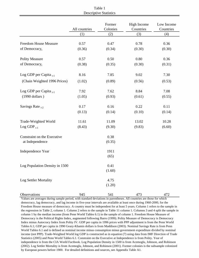
All countriesFormer

ColoniesHigh Income

CountriesLow Income

Countries(1) (2) (3) (4)

Freedom House Measure 0.57 0.47 0.78 0.36of Democracyt (0.36) (0.34) (0.30) (0.30)

Polity Measure 0.57 0.50 0.80 0.36of Democracyt (0.38) (0.35) (0.30) (0.31)

Log GDP per Capita t-1 8.16 7.85 9.02 7.30

(Chain Weighted 1996 Prices) (1.02) (0.89) (0.56) (0.53)

Log GDP per Capita t-1 7.92 7.62 8.84 7.08 (1990 dollars ) (1.05) (0.93) (0.61) (0.55)

Savings Rate t-2 0.17 0.16 0.22 0.11(0.13) (0.14) (0.10) (0.14)

Trade-Weighted World 11.61 11.09 13.02 10.28Log GDP t-1 (8.43) (9.30) (9.83) (6.60)

Constraint on the Executive 0.38 at Independence (0.35)

Independence Year 1911(65)

Log Population Density in 1500 0.41(1.60)

Log Settler Mortality 4.75(1.20)

Observations 945 541 473 472

Table 1Descriptive Statistics

Values are averages during sample period, with standard deviations in parentheses. All countries are those for which democracy, lag democracy, and lag income in five-year intervals are available at least once during 1960-2000, for the Freedom House measure of democracy. A country must be independent for at least 5 years. Column 1 refers to the sample in the regression in Table 2, column 1. Column 2 refers to the sample in Table 11 column 1. Columns 3 and 4 split the sample in column 1 by the median income (from Penn World Tables 6.1) in the sample of column 1. Freedom House Measure of Democracy is the Political Rights Index, augmented following Barro (1999). Polity Measure of Democracy is Democracy Index minus Autocracy Index from Polity IV. GDP per capita in 1996 prices with PPP adjustment is from the Penn World Tables 6.1; GDP per capita in 1990 Geary-Khamis dollars is from Maddison (2003). Nominal Savings Rate is from Penn World Tables 6.1 and is defined as nominal income minus consumption minus government expenditure divided by nominal income (not PPP). Trade-Weighted World log GDP is constructed as in equation (7) using data from IMF Direction of Trade Statistics (2005) and Penn World Tables 6.1. Constraint on the Executive at Independence is from Polity. Year of independence is from the CIA World Factbook. Log Population Density in 1500 is from Acemoglu, Johnson, and Robinson (2002). Log Settler Mortality is from Acemoglu, Johnson, and Robinson (2001). Former colonies is the subsample colonized by European powers before 1900. For detailed definitions and sources, see Appendix Table A1.

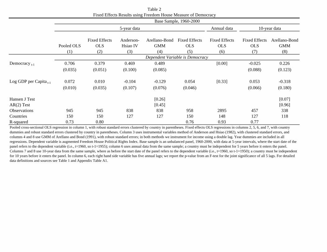
Annual data

Pooled OLSFixed Effects

OLSAnderson-Hsiao IV

Arellano-Bond GMM

Fixed Effects OLS

Fixed Effects OLS

Fixed Effects OLS

Arellano-Bond GMM

(1) (2) (3) (4) (5) (6) (7) (8)

Democracy t-1 0.706 0.379 0.469 0.489 [0.00] -0.025 0.226(0.035) (0.051) (0.100) (0.085) (0.088) (0.123)

Log GDP per Capita t-1 0.072 0.010 -0.104 -0.129 0.054 [0.33] 0.053 -0.318(0.010) (0.035) (0.107) (0.076) (0.046) (0.066) (0.180)

Hansen J Test [0.26] [0.07]AR(2) Test [0.45] [0.96]Observations 945 945 838 838 958 2895 457 338Countries 150 150 127 127 150 148 127 118R-squared 0.73 0.80 0.76 0.93 0.77

Dependent Variable is Democracy

Table 2Fixed Effects Results using Freedom House Measure of Democracy

Base Sample, 1960-20005-year data 10-year data

Pooled cross-sectional OLS regression in column 1, with robust standard errors clustered by country in parentheses. Fixed effects OLS regressions in columns 2, 5, 6, and 7, with country dummies and robust standard errors clustered by country in parentheses. Column 3 uses instrumental variables method of Anderson and Hsiao (1982), with clustered standard errors, and columns 4 and 8 use GMM of Arellano and Bond (1991), with robust standard errors; in both methods we instrument for income using a double lag. Year dummies are included in all regressions. Dependent variable is augmented Freedom House Political Rights Index. Base sample is an unbalanced panel, 1960-2000, with data at 5-year intervals, where the start date of the panel refers to the dependent variable (i.e., t=1960, so t-1=1955); column 6 uses annual data from the same sample; a country must be independent for 5 years before it enters the panel. Columns 7 and 8 use 10-year data from the same sample, where as before the start date of the panel refers to the dependent variable (i.e., t=1960, so t-1=1950); a country must be independent for 10 years before it enters the panel. In column 6, each right hand side variable has five annual lags; we report the p-value from an F-test for the joint significance of all 5 lags. For detailed data definitions and sources see Table 1 and Appendix Table A1.

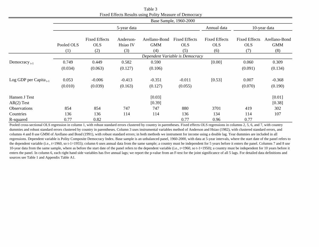
Annual data

Pooled OLSFixed Effects

OLSAnderson-Hsiao IV

Arellano-Bond GMM

Fixed Effects OLS

Fixed Effects OLS

Fixed Effects OLS

Arellano-Bond GMM

(1) (2) (3) (4) (5) (6) (7) (8)

Democracy t-1 0.749 0.449 0.582 0.590 [0.00] 0.060 0.309(0.034) (0.063) (0.127) (0.106) (0.091) (0.134)

Log GDP per Capita t-1 0.053 -0.006 -0.413 -0.351 -0.011 [0.53] 0.007 -0.368(0.010) (0.039) (0.163) (0.127) (0.055) (0.070) (0.190)

Hansen J Test [0.03] [0.01]AR(2) Test [0.39] [0.38]Observations 854 854 747 747 880 3701 419 302Countries 136 136 114 114 136 134 114 107R-squared 0.77 0.82 0.77 0.96 0.77

Dependent Variable is Democracy

Table 3Fixed Effects Results using Polity Measure of Democracy

Base Sample, 1960-20005-year data 10-year data

Pooled cross-sectional OLS regression in column 1, with robust standard errors clustered by country in parentheses. Fixed effects OLS regressions in columns 2, 5, 6, and 7, with country dummies and robust standard errors clustered by country in parentheses. Column 3 uses instrumental variables method of Anderson and Hsiao (1982), with clustered standard errors, and columns 4 and 8 use GMM of Arellano and Bond (1991), with robust standard errors; in both methods we instrument for income using a double lag. Year dummies are included in all regressions. Dependent variable is Polity Composite Democracy Index. Base sample is an unbalanced panel, 1960-2000, with data at 5-year intervals, where the start date of the panel refers to the dependent variable (i.e., t=1960, so t-1=1955); column 6 uses annual data from the same sample; a country must be independent for 5 years before it enters the panel. Columns 7 and 8 use 10-year data from the same sample, where as before the start date of the panel refers to the dependent variable (i.e., t=1960, so t-1=1950); a country must be independent for 10 years before it enters the panel. In column 6, each right hand side variables has five annual lags; we report the p-value from an F-test for the joint significance of all 5 lags. For detailed data definitions and sources see Table 1 and Appendix Table A1.

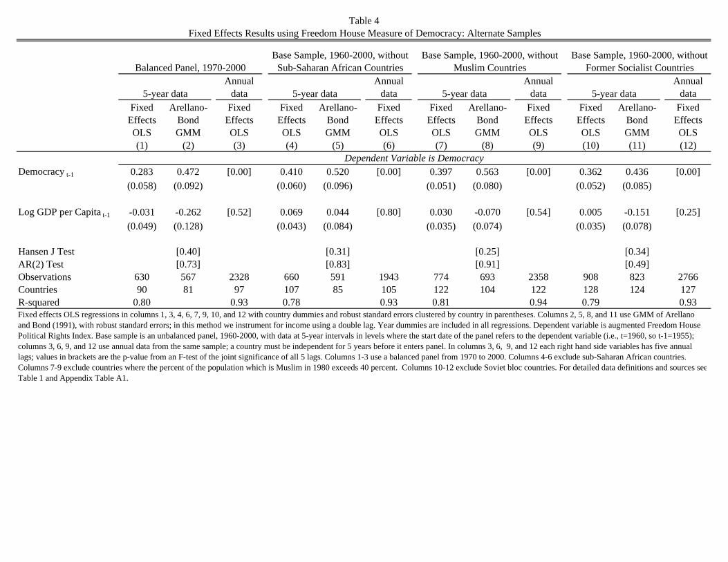
Annual data

Annual data

Annual data

Annual data

Fixed Effects OLS

Arellano-Bond GMM

Fixed Effects OLS

Fixed Effects OLS

Arellano-Bond GMM

Fixed Effects OLS

Fixed Effects OLS

Arellano-Bond GMM

Fixed Effects OLS

Fixed Effects OLS

Arellano-Bond GMM

Fixed Effects OLS

(1) (2) (3) (4) (5) (6) (7) (8) (9) (10) (11) (12)

Democracy t-1 0.283 0.472 [0.00] 0.410 0.520 [0.00] 0.397 0.563 [0.00] 0.362 0.436 [0.00](0.058) (0.092) (0.060) (0.096) (0.051) (0.080) (0.052) (0.085)

Log GDP per Capita t-1 -0.031 -0.262 [0.52] 0.069 0.044 [0.80] 0.030 -0.070 [0.54] 0.005 -0.151 [0.25](0.049) (0.128) (0.043) (0.084) (0.035) (0.074) (0.035) (0.078)

Hansen J Test [0.40] [0.31] [0.25] [0.34]AR(2) Test [0.73] [0.83] [0.91] [0.49]Observations 630 567 2328 660 591 1943 774 693 2358 908 823 2766Countries 90 81 97 107 85 105 122 104 122 128 124 127R-squared 0.80 0.93 0.78 0.93 0.81 0.94 0.79 0.93

5-year data 5-year data

Base Sample, 1960-2000, without Former Socialist Countries

5-year data

Base Sample, 1960-2000, without Muslim Countries

Base Sample, 1960-2000, without Sub-Saharan African Countries

5-year data

Balanced Panel, 1970-2000

Table 4

Dependent Variable is Democracy

Fixed Effects Results using Freedom House Measure of Democracy: Alternate Samples

Fixed effects OLS regressions in columns 1, 3, 4, 6, 7, 9, 10, and 12 with country dummies and robust standard errors clustered by country in parentheses. Columns 2, 5, 8, and 11 use GMM of Arellano and Bond (1991), with robust standard errors; in this method we instrument for income using a double lag. Year dummies are included in all regressions. Dependent variable is augmented Freedom House Political Rights Index. Base sample is an unbalanced panel, 1960-2000, with data at 5-year intervals in levels where the start date of the panel refers to the dependent variable (i.e., t=1960, so t-1=1955); columns 3, 6, 9, and 12 use annual data from the same sample; a country must be independent for 5 years before it enters panel. In columns 3, 6, 9, and 12 each right hand side variables has five annual lags; values in brackets are the p-value from an F-test of the joint significance of all 5 lags. Columns 1-3 use a balanced panel from 1970 to 2000. Columns 4-6 exclude sub-Saharan African countries. Columns 7-9 exclude countries where the percent of the population which is Muslim in 1980 exceeds 40 percent. Columns 10-12 exclude Soviet bloc countries. For detailed data definitions and sources seeTable 1 and Appendix Table A1.

Pooled OLSFixed Effects

OLSArellano-

Bond GMM Pooled OLSFixed Effects

OLSArellano-

Bond GMM Pooled OLSFixed Effects

OLSArellano-

Bond GMM(1) (2) (3) (4) (5) (6) (7) (8) (9)

Democracy t-1 0.687 0.353 0.480 0.625 0.351 0.499 0.619 0.352 0.475(0.039) (0.053) (0.087) (0.044) (0.055) (0.097) (0.042) (0.050) (0.088)

Log GDP per Capita t-1 0.066 0.015 -0.008 0.047 -0.001 -0.121 0.061 -0.042 -0.126(0.014) (0.041) (0.139) (0.020) (0.049) (0.182) (0.017) (0.045) (0.130)

Log Population t-1 0.001 -0.109 -0.001 -0.001 -0.042 0.049 0.005 -0.070 -0.016(0.005) (0.100) (0.113) (0.006) (0.108) (0.143) (0.006) (0.112) (0.163)

Education t-1 0.012 -0.007 -0.020 0.022 -0.006 -0.011(0.005) (0.020) (0.026) (0.007) (0.038) (0.052)

Age Structure t-1 [0.00] [0.05] [0.63] [0.06] [0.19] [0.27]

Barro (1999) Covariates NO NO NO NO NO NO YES YES YES

Hansen J Test [0.08] [0.15] [0.25]AR(2) Test [0.43] [0.88] [0.75]Observations 863 863 731 676 676 589 676 676 588Countries 142 142 120 95 95 92 96 96 92R-squared 0.72 0.80 0.70 0.77 0.70 0.76

Dependent Variable is Democracy

Fixed Effects Results using Freedom House Measure of Democracy: Alternate CovariatesTable 5

Base Sample, 1960-20005-year data

Pooled cross-sectional OLS regressions in columns 1, 4, and 7, with robust standard errors clustered by country in parentheses. Fixed effects OLS regressions in columns 2, 6, and 8, with country dummies and robust standard errors clustered by country in parentheses. GMM of Arellano-Bond in columns 3, 6, and 9, with robust standard errors; in this method we instrument for income using a double lag. Year dummies are included in all regressions. Dependent variable is augmented Freedom House Political Rights Index. Base sample is an unbalanced panel, 1960-2000, with data at 5-year intervals, where the start date of the panel refers to the dependent variable (i.e., t=1960, so t-1=1955); a country must be independent for 5 years before it enters the panel. Education is average years of total schooling in the population in columns 4-6. Education is average years of primary schooling in the population in columns 7-9. Columns 1-6 include but do not display the median age of the population at t-1 and 4 covariates corresponding to the percent of the population at t-1 in the following age groups: 0-15, 15-30, 30-45, and 45-60. The age structure F-test is gives the p-value for the joint significance of these variables. Columns 7-9 include but do not display additional covariates used by Barro (1999): male-female education gap and urbanization rate, and significant oil producer dummy (the last is in column 7 only). For detailed data definitions and sources see Table 1 and Appendix Table A1.

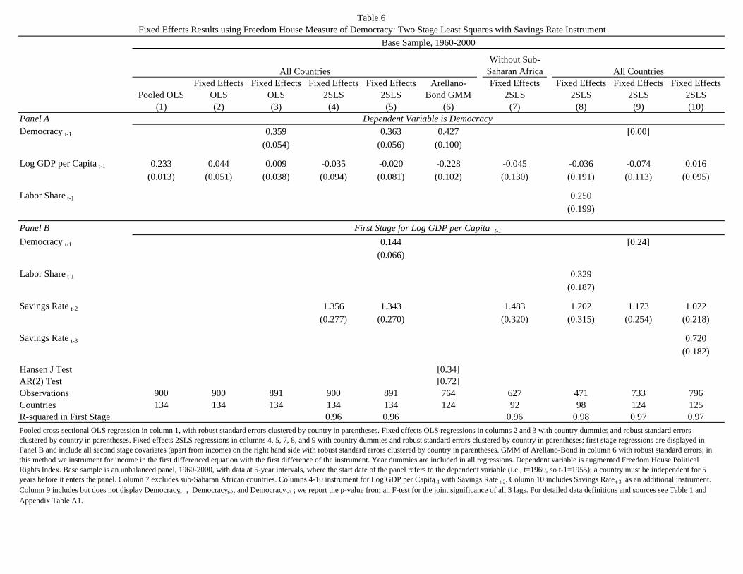
Without Sub-Saharan Africa

Pooled OLSFixed Effects

OLSFixed Effects

OLSFixed Effects

2SLSFixed Effects

2SLSArellano-

Bond GMMFixed Effects

2SLSFixed Effects

2SLSFixed Effects

2SLSFixed Effects

2SLS(1) (2) (3) (4) (5) (6) (7) (8) (9) (10)

Panel ADemocracy t-1 0.359 0.363 0.427 [0.00]

(0.054) (0.056) (0.100)

Log GDP per Capita t-1 0.233 0.044 0.009 -0.035 -0.020 -0.228 -0.045 -0.036 -0.074 0.016(0.013) (0.051) (0.038) (0.094) (0.081) (0.102) (0.130) (0.191) (0.113) (0.095)

Labor Share t-1 0.250(0.199)

Panel BDemocracy t-1 0.144 [0.24]

(0.066)

Labor Share t-1 0.329(0.187)

Savings Rate t-2 1.356 1.343 1.483 1.202 1.173 1.022(0.277) (0.270) (0.320) (0.315) (0.254) (0.218)

Savings Rate t-3 0.720(0.182)

Hansen J Test [0.34]AR(2) Test [0.72]Observations 900 900 891 900 891 764 627 471 733 796Countries 134 134 134 134 134 124 92 98 124 125R-squared in First Stage 0.96 0.96 0.96 0.98 0.97 0.97

Table 6Fixed Effects Results using Freedom House Measure of Democracy: Two Stage Least Squares with Savings Rate Instrument

Dependent Variable is Democracy

First Stage for Log GDP per Capita t-1

All Countries All Countries

Base Sample, 1960-2000

Pooled cross-sectional OLS regression in column 1, with robust standard errors clustered by country in parentheses. Fixed effects OLS regressions in columns 2 and 3 with country dummies and robust standard errors clustered by country in parentheses. Fixed effects 2SLS regressions in columns 4, 5, 7, 8, and 9 with country dummies and robust standard errors clustered by country in parentheses; first stage regressions are displayed in Panel B and include all second stage covariates (apart from income) on the right hand side with robust standard errors clustered by country in parentheses. GMM of Arellano-Bond in column 6 with robust standard errors; in this method we instrument for income in the first differenced equation with the first difference of the instrument. Year dummies are included in all regressions. Dependent variable is augmented Freedom House Political Rights Index. Base sample is an unbalanced panel, 1960-2000, with data at 5-year intervals, where the start date of the panel refers to the dependent variable (i.e., t=1960, so t-1=1955); a country must be independent for 5 years before it enters the panel. Column 7 excludes sub-Saharan African countries. Columns 4-10 instrument for Log GDP per Capita t-1 with Savings Rate t-2. Column 10 includes Savings Rate t-3 as an additional instrument.Column 9 includes but does not display Democracyt-1 , Democracyt-2, and Democracyt-3 ; we report the p-value from an F-test for the joint significance of all 3 lags. For detailed data definitions and sources see Table 1 and Appendix Table A1.

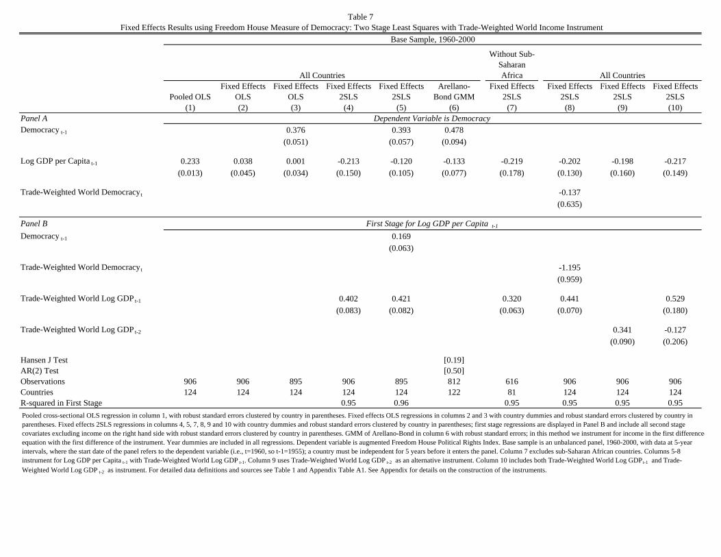
Without Sub-Saharan Africa

Pooled OLSFixed Effects

OLSFixed Effects

OLSFixed Effects

2SLSFixed Effects

2SLSArellano-

Bond GMMFixed Effects

2SLSFixed Effects

2SLSFixed Effects

2SLSFixed Effects

2SLS(1) (2) (3) (4) (5) (6) (7) (8) (9) (10)

Panel ADemocracy t-1 0.376 0.393 0.478

(0.051) (0.057) (0.094)

Log GDP per Capita t-1 0.233 0.038 0.001 -0.213 -0.120 -0.133 -0.219 -0.202 -0.198 -0.217(0.013) (0.045) (0.034) (0.150) (0.105) (0.077) (0.178) (0.130) (0.160) (0.149)

Trade-Weighted World Democracy t -0.137(0.635)

Panel BDemocracy t-1 0.169

(0.063)

Trade-Weighted World Democracy t -1.195(0.959)

Trade-Weighted World Log GDP t-1 0.402 0.421 0.320 0.441 0.529(0.083) (0.082) (0.063) (0.070) (0.180)

Trade-Weighted World Log GDP t-2 0.341 -0.127(0.090) (0.206)

Hansen J Test [0.19]AR(2) Test [0.50]Observations 906 906 895 906 895 812 616 906 906 906Countries 124 124 124 124 124 122 81 124 124 124R-squared in First Stage 0.95 0.96 0.95 0.95 0.95 0.95

Table 7Fixed Effects Results using Freedom House Measure of Democracy: Two Stage Least Squares with Trade-Weighted World Income Instrument

Dependent Variable is Democracy

First Stage for Log GDP per Capita t-1

All Countries

Base Sample, 1960-2000

All Countries

Pooled cross-sectional OLS regression in column 1, with robust standard errors clustered by country in parentheses. Fixed effects OLS regressions in columns 2 and 3 with country dummies and robust standard errors clustered by country in parentheses. Fixed effects 2SLS regressions in columns 4, 5, 7, 8, 9 and 10 with country dummies and robust standard errors clustered by country in parentheses; first stage regressions are displayed in Panel B and include all second stage covariates excluding income on the right hand side with robust standard errors clustered by country in parentheses. GMM of Arellano-Bond in column 6 with robust standard errors; in this method we instrument for income in the first differencedequation with the first difference of the instrument. Year dummies are included in all regressions. Dependent variable is augmented Freedom House Political Rights Index. Base sample is an unbalanced panel, 1960-2000, with data at 5-year intervals, where the start date of the panel refers to the dependent variable (i.e., t=1960, so t-1=1955); a country must be independent for 5 years before it enters the panel. Column 7 excludes sub-Saharan African countries. Columns 5-8 instrument for Log GDP per Capita t-1 with Trade-Weighted World Log GDP t-1. Column 9 uses Trade-Weighted World Log GDP t-2 as an alternative instrument. Column 10 includes both Trade-Weighted World Log GDP t-1 and Trade-Weighted World Log GDP t-2 as instrument. For detailed data definitions and sources see Table 1 and Appendix Table A1. See Appendix for details on the construction of the instruments.

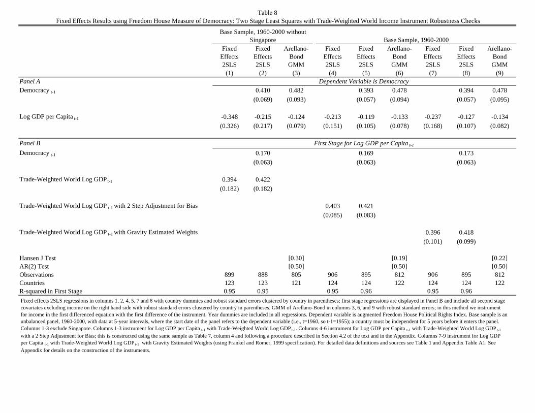
Fixed Effects 2SLS

Fixed Effects 2SLS

Arellano-Bond GMM

Fixed Effects 2SLS

Fixed Effects 2SLS

Arellano-Bond GMM

Fixed Effects 2SLS

Fixed Effects 2SLS

Arellano-Bond GMM

(1) (2) (3) (4) (5) (6) (7) (8) (9)Panel ADemocracy t-1 0.410 0.482 0.393 0.478 0.394 0.478

(0.069) (0.093) (0.057) (0.094) (0.057) (0.095)

Log GDP per Capita t-1 -0.348 -0.215 -0.124 -0.213 -0.119 -0.133 -0.237 -0.127 -0.134(0.326) (0.217) (0.079) (0.151) (0.105) (0.078) (0.168) (0.107) (0.082)

Panel BDemocracy t-1 0.170 0.169 0.173

(0.063) (0.063) (0.063)

Trade-Weighted World Log GDP t-1 0.394 0.422(0.182) (0.182)

Trade-Weighted World Log GDP t-1 with 2 Step Adjustment for Bias 0.403 0.421(0.085) (0.083)

Trade-Weighted World Log GDP t-1 with Gravity Estimated Weights 0.396 0.418(0.101) (0.099)

Hansen J Test [0.30] [0.19] [0.22]AR(2) Test [0.50] [0.50] [0.50]Observations 899 888 805 906 895 812 906 895 812Countries 123 123 121 124 124 122 124 124 122R-squared in First Stage 0.95 0.95 0.95 0.96 0.95 0.96

Table 8Fixed Effects Results using Freedom House Measure of Democracy: Two Stage Least Squares with Trade-Weighted World Income Instrument Robustness Checks

Dependent Variable is Democracy

First Stage for Log GDP per Capita t-1

Base Sample, 1960-2000Base Sample, 1960-2000 without

Singapore

Fixed effects 2SLS regressions in columns 1, 2, 4, 5, 7 and 8 with country dummies and robust standard errors clustered by country in parentheses; first stage regressions are displayed in Panel B and include all second stage covariates excluding income on the right hand side with robust standard errors clustered by country in parentheses. GMM of Arellano-Bond in columns 3, 6, and 9 with robust standard errors; in this method we instrument for income in the first differenced equation with the first difference of the instrument. Year dummies are included in all regressions. Dependent variable is augmented Freedom House Political Rights Index. Base sample is an unbalanced panel, 1960-2000, with data at 5-year intervals, where the start date of the panel refers to the dependent variable (i.e., t=1960, so t-1=1955); a country must be independent for 5 years before it enters the panel. Columns 1-3 exclude Singapore. Columns 1-3 instrument for Log GDP per Capita t-1 with Trade-Weighted World Log GDP t-1. Columns 4-6 instrument for Log GDP per Capita t-1 with Trade-Weighted World Log GDP t-1

with a 2 Step Adjustment for Bias; this is constructed using the same sample as Table 7, column 4 and following a procedure described in Section 4.2 of the text and in the Appendix. Columns 7-9 instrument for Log GDP per Capita t-1 with Trade-Weighted World Log GDP t-1 with Gravity Estimated Weights (using Frankel and Romer, 1999 specification). For detailed data definitions and sources see Table 1 and Appendix Table A1. See Appendix for details on the construction of the instruments.

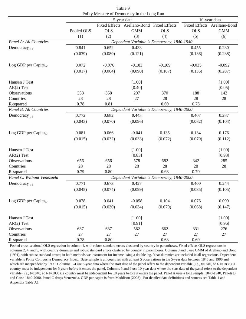
Pooled OLSFixed Effects

OLSArellano-Bond

GMMFixed Effects

OLSFixed Effects

OLSArellano-Bond

GMM(1) (2) (3) (4) (5) (6)

Panel A: All CountriesDemocracy t-1 0.841 0.652 0.433 0.455 0.230

(0.039) (0.089) (0.121) (0.136) (0.238)

Log GDP per Capita t-1 0.072 -0.076 -0.183 -0.109 -0.035 -0.092(0.017) (0.064) (0.090) (0.107) (0.135) (0.287)

Hansen J Test [1.00] [1.00]AR(2) Test [0.40] [0.05]Observations 358 358 297 370 188 142Countries 28 28 27 28 28 28R-squared 0.78 0.81 0.69 0.75Panel B: All CountriesDemocracy t-1 0.772 0.682 0.443 0.407 0.287

(0.043) (0.070) (0.096) (0.082) (0.104)

Log GDP per Capita t-1 0.081 0.066 -0.041 0.135 0.134 0.176(0.015) (0.032) (0.033) (0.072) (0.070) (0.112)

Hansen J Test [1.00] [1.00]AR(2) Test [0.83] [0.93]Observations 656 656 578 682 342 285Countries 28 28 28 28 28 28R-squared 0.79 0.80 0.63 0.70Panel C: Without VenezuelaDemocracy t-1 0.771 0.673 0.427 0.400 0.244

(0.045) (0.074) (0.099) (0.085) (0.105)

Log GDP per Capita t-1 0.078 0.041 -0.058 0.104 0.076 0.099(0.015) (0.030) (0.034) (0.079) (0.068) (0.147)

Hansen J Test [1.00] [1.00]AR(2) Test [0.91] [0.96]Observations 637 637 562 662 331 276Countries 27 27 27 27 27 27R-squared 0.78 0.80 0.63 0.69

Table 9Polity Measure of Democracy in the Long Run

Dependent Variable is Democracy, 1840-2000

Dependent Variable is Democracy, 1840-2000

Dependent Variable is Democracy, 1840-1940

10-year data5-year data

Pooled cross-sectional OLS regression in column 1, with robust standard errors clustered by country in parentheses. Fixed effects OLS regressions in columns 2, 4, and 5, with country dummies and robust standard errors clustered by country in parentheses. Column 3 and 6 use GMM of Arellano and Bond (1991), with robust standard errors; in both methods we instrument for income using a double lag. Year dummies are included in all regressions. Dependent variable is Polity Composite Democracy Index. Base sample is all countries with at least 5 observations in the 5-year data between 1840 and 1900 and which are independent by 1900. Columns 1-4 use 5-year data where the start date of the panel refers to the dependent variable (i.e., t=1840, so t-1=1835); a country must be independent for 5 years before it enters the panel. Columns 5 and 6 use 10-year data where the start date of the panel refers to the dependent variable (i.e., t=1840, so t-1=1830); a country must be independent for 10 years before it enters the panel. Panel A uses a long sample, 1840-1940, Panels B and C use 1840-2000. Panel C drops Venezuela. GDP per capita is from Maddison (2003). For detailed data definitions and sources see Table 1 and Appendix Table A1.

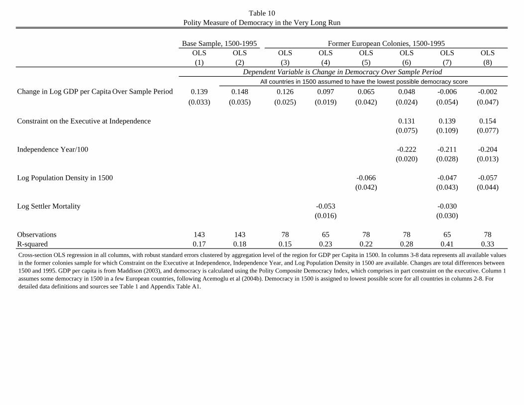
OLS OLS OLS OLS OLS OLS OLS OLS(1) (2) (3) (4) (5) (6) (7) (8)

Change in Log GDP per Capita Over Sample Period 0.139 0.148 0.126 0.097 0.065 0.048 -0.006 -0.002(0.033) (0.035) (0.025) (0.019) (0.042) (0.024) (0.054) (0.047)

Constraint on the Executive at Independence 0.131 0.139 0.154(0.075) (0.109) (0.077)

Independence Year/100 -0.222 -0.211 -0.204(0.020) (0.028) (0.013)

Log Population Density in 1500 -0.066 -0.047 -0.057(0.042) (0.043) (0.044)

Log Settler Mortality -0.053 -0.030(0.016) (0.030)

Observations 143 143 78 65 78 78 65 78R-squared 0.17 0.18 0.15 0.23 0.22 0.28 0.41 0.33

Table 10Polity Measure of Democracy in the Very Long Run

Former European Colonies, 1500-1995Base Sample, 1500-1995

Dependent Variable is Change in Democracy Over Sample PeriodAll countries in 1500 assumed to have the lowest possible democracy score

Cross-section OLS regression in all columns, with robust standard errors clustered by aggregation level of the region for GDP per Capita in 1500. In columns 3-8 data represents all available values in the former colonies sample for which Constraint on the Executive at Independence, Independence Year, and Log Population Density in 1500 are available. Changes are total differences between 1500 and 1995. GDP per capita is from Maddison (2003), and democracy is calculated using the Polity Composite Democracy Index, which comprises in part constraint on the executive. Column 1 assumes some democracy in 1500 in a few European countries, following Acemoglu et al (2004b). Democracy in 1500 is assigned to lowest possible score for all countries in columns 2-8. For detailed data definitions and sources see Table 1 and Appendix Table A1.

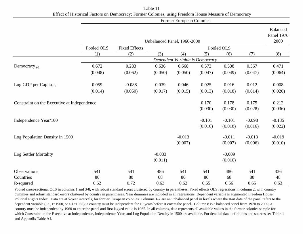
Balanced Panel 1970-

2000Pooled OLS Fixed Effects

(1) (2) (3) (4) (5) (6) (7) (8)

Democracy t-1 0.672 0.283 0.636 0.668 0.573 0.538 0.567 0.471(0.048) (0.062) (0.050) (0.050) (0.047) (0.049) (0.047) (0.064)

Log GDP per Capita t-1 0.059 -0.088 0.039 0.046 0.025 0.016 0.012 0.008(0.014) (0.050) (0.017) (0.015) (0.013) (0.018) (0.014) (0.020)

Constraint on the Executive at Independence 0.170 0.178 0.175 0.212(0.030) (0.030) (0.028) (0.036)

Independence Year/100 -0.101 -0.101 -0.098 -0.135(0.016) (0.018) (0.016) (0.022)

Log Population Density in 1500 -0.013 -0.011 -0.013 -0.019(0.007) (0.007) (0.006) (0.010)

Log Settler Mortality -0.033 -0.009(0.011) (0.010)

Observations 541 541 486 541 541 486 541 336Countries 80 80 68 80 80 68 80 48R-squared 0.62 0.72 0.63 0.62 0.65 0.66 0.65 0.63

Table 11Effect of Historical Factors on Democracy: Former Colonies, using Freedom House Measure of Democracy

Dependent Variable is Democracy

Former European Colonies

Pooled OLSUnbalanced Panel, 1960-2000

Pooled cross-sectional OLS in columns 1 and 3-8, with robust standard errors clustered by country in parentheses. Fixed effects OLS regressions in column 2, with country dummies and robust standard errors clustered by country in parentheses. Year dummies are included in all regressions. Dependent variable is augmented Freedom House Political Rights Index. Data are at 5-year intervals, for former European colonies. Columns 1-7 are an unbalanced panel in levels where the start date of the panel refers to the dependent variable (i.e., t=1960, so t-1=1955); a country must be independent for 10 years before it enters the panel. Column 8 is a balanced panel from 1970 to 2000; a country must be independent by 1960 to enter the panel and first lagged value is 1965. In all columns, data represents all available values in the former colonies sample for which Constraint on the Executive at Independence, Independence Year, and Log Population Density in 1500 are available. For detailed data definitions and sources see Table 1 and Appendix Table A1.

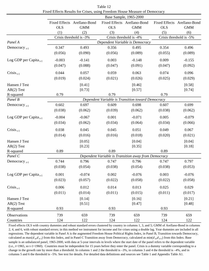
Fixed Effects OLS

Arellano-Bond GMM

Fixed Effects OLS

Arellano-Bond GMM

Fixed Effects OLS

Arellano-Bond GMM

(1) (2) (3) (4) (5) (6)

Panel ADemocracy t-1 0.347 0.493 0.356 0.495 0.354 0.496

(0.056) (0.090) (0.056) (0.089) (0.055) (0.089)

Log GDP per Capita t-1 -0.003 -0.141 0.003 -0.148 0.009 -0.155(0.047) (0.088) (0.047) (0.091) (0.047) (0.092)

Crisis t-1 0.044 0.057 0.059 0.063 0.074 0.096(0.019) (0.024) (0.021) (0.026) (0.025) (0.029)

Hansen J Test [0.41] [0.46] [0.58]AR(2) Test [0.73] [0.57] [0.74]R-squared 0.79 0.79 0.79Panel BDemocracy t-1 0.602 0.697 0.609 0.698 0.607 0.699

(0.038) (0.062) (0.039) (0.062) (0.038) (0.062)

Log GDP per Capita t-1 -0.004 -0.067 0.001 -0.071 0.005 -0.079(0.034) (0.062) (0.034) (0.064) (0.034) (0.066)

Crisis t-1 0.038 0.045 0.045 0.051 0.049 0.067(0.014) (0.016) (0.016) (0.018) (0.020) (0.021)

Hansen J Test [0.05] [0.04] [0.04]AR(2) Test [0.23] [0.35] [0.18]R-squared 0.89 0.89 0.89Panel CDemocracy t-1 0.744 0.796 0.747 0.796 0.747 0.797

(0.038) (0.054) (0.038) (0.054) (0.038) (0.053)

Log GDP per Capita t-1 0.001 -0.074 0.002 -0.076 0.003 -0.076(0.023) (0.057) (0.022) (0.058) (0.022) (0.058)

Crisis t-1 0.006 0.012 0.014 0.013 0.025 0.029(0.011) (0.014) (0.011) (0.015) (0.011) (0.017)

Hansen J Test [0.14] [0.16] [0.21]AR(2) Test [0.51] [0.47] [0.48]R-squared 0.93 0.93 0.93

Observations 739 659 739 659 739 659Countries 124 122 124 122 124 122

Dependent Variable is Transition toward Democracy

Dependent Variable is Transition away from Democracy

Table 12Fixed Effects Results for Crises, using Freedom House Measure of Democracy

Dependent Variable is Democracy

Base Sample, 1965-2000

Crisis threshold is -3% Crisis threshold is -4% Crisis threshold is -5%

Fixed effects OLS with country dummies and robust standard errors clustered by country in columns 1, 3, and 5; GMM of Arellano-Bond in columns 2, 4, and 6, with robust standard errors; in this method we instrument for income and for crises using a double lag. Year dummies are included in all regressions. The dependent variable in Panel A is the augmented Freedom House Political Rights Index, in Panel B, Transition towards Democracy, calculated as max(d it,d it-1) from this Index, and in Panel C Transition away from Democracy, calculated as min(d it,d it-1) from this Index. Base sample is an unbalanced panel, 1965-2000, with data at 5-year intervals in levels where the start date of the panel refers to the dependent variable (i.e., t=1965, so t-1=1960). Countries must be independent for 15 years before they enter the panel. Crisis is a dummy variable corresponding to a change in the growth rate by more than a threshold. In columns 1 and 2 the threshold is –3%, in columns 3 and 4 the threshold is –4%, and in columns 5 and 6 the threshold is –5%. See text for details. For detailed data definitions and sources see Table 1 and Appendix Table A1.

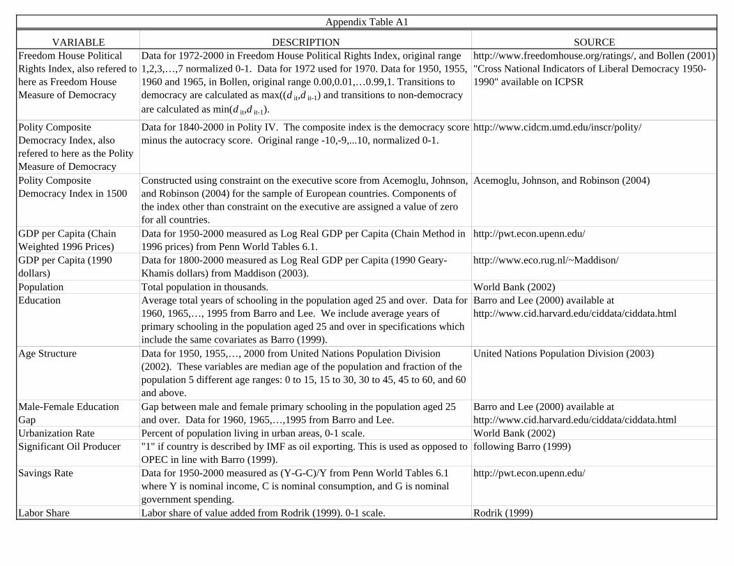
VARIABLE DESCRIPTION SOURCEFreedom House Political Rights Index, also refered to here as Freedom House Measure of Democracy

Data for 1972-2000 in Freedom House Political Rights Index, original range 1,2,3,…,7 normalized 0-1. Data for 1972 used for 1970. Data for 1950, 1955, 1960 and 1965, in Bollen, original range 0.00,0.01,…0.99,1. Transitions to democracy are calculated as max((d it,d it-1) and transitions to non-democracy are calculated as min(d it,d it-1).

http://www.freedomhouse.org/ratings/, and Bollen (2001) "Cross National Indicators of Liberal Democracy 1950-1990" available on ICPSR

Polity Composite Democracy Index, also refered to here as the Polity Measure of Democracy

Data for 1840-2000 in Polity IV. The composite index is the democracy score minus the autocracy score. Original range -10,-9,...10, normalized 0-1.

http://www.cidcm.umd.edu/inscr/polity/

Polity Composite Democracy Index in 1500

Constructed using constraint on the executive score from Acemoglu, Johnson, and Robinson (2004) for the sample of European countries. Components of the index other than constraint on the executive are assigned a value of zero for all countries.

Acemoglu, Johnson, and Robinson (2004)

GDP per Capita (Chain Weighted 1996 Prices)

Data for 1950-2000 measured as Log Real GDP per Capita (Chain Method in 1996 prices) from Penn World Tables 6.1.

http://pwt.econ.upenn.edu/

GDP per Capita (1990 dollars)

Data for 1800-2000 measured as Log Real GDP per Capita (1990 Geary-Khamis dollars) from Maddison (2003).

http://www.eco.rug.nl/~Maddison/

Population Total population in thousands. World Bank (2002)Education Average total years of schooling in the population aged 25 and over. Data for

1960, 1965,…, 1995 from Barro and Lee. We include average years of primary schooling in the population aged 25 and over in specifications which include the same covariates as Barro (1999).

Barro and Lee (2000) available at http://www.cid.harvard.edu/ciddata/ciddata.html

Age Structure Data for 1950, 1955,…, 2000 from United Nations Population Division (2002). These variables are median age of the population and fraction of the population 5 different age ranges: 0 to 15, 15 to 30, 30 to 45, 45 to 60, and 60 and above.

United Nations Population Division (2003)

Male-Female Education Gap

Gap between male and female primary schooling in the population aged 25 and over. Data for 1960, 1965,…,1995 from Barro and Lee.

Barro and Lee (2000) available at http://www.cid.harvard.edu/ciddata/ciddata.html

Urbanization Rate Percent of population living in urban areas, 0-1 scale. World Bank (2002)Significant Oil Producer "1" if country is described by IMF as oil exporting. This is used as opposed to

OPEC in line with Barro (1999).following Barro (1999)

Savings Rate Data for 1950-2000 measured as (Y-G-C)/Y from Penn World Tables 6.1 where Y is nominal income, C is nominal consumption, and G is nominal government spending.

http://pwt.econ.upenn.edu/

Labor Share Labor share of value added from Rodrik (1999). 0-1 scale. Rodrik (1999)

Appendix Table A1

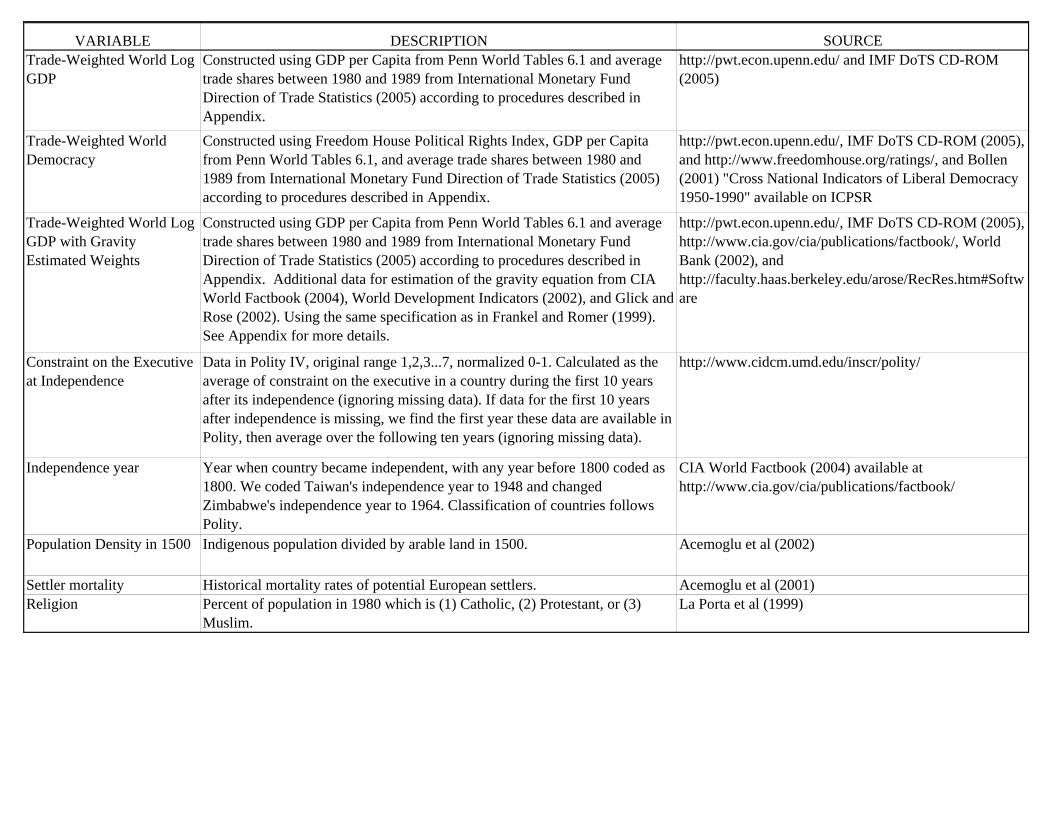
VARIABLE DESCRIPTION SOURCETrade-Weighted World Log GDP

Constructed using GDP per Capita from Penn World Tables 6.1 and average trade shares between 1980 and 1989 from International Monetary Fund Direction of Trade Statistics (2005) according to procedures described in Appendix.

http://pwt.econ.upenn.edu/ and IMF DoTS CD-ROM (2005)

Trade-Weighted World Democracy

Constructed using Freedom House Political Rights Index, GDP per Capita from Penn World Tables 6.1, and average trade shares between 1980 and 1989 from International Monetary Fund Direction of Trade Statistics (2005) according to procedures described in Appendix.

http://pwt.econ.upenn.edu/, IMF DoTS CD-ROM (2005), and http://www.freedomhouse.org/ratings/, and Bollen (2001) "Cross National Indicators of Liberal Democracy 1950-1990" available on ICPSR

Trade-Weighted World Log GDP with Gravity Estimated Weights

Constructed using GDP per Capita from Penn World Tables 6.1 and average trade shares between 1980 and 1989 from International Monetary Fund Direction of Trade Statistics (2005) according to procedures described in Appendix. Additional data for estimation of the gravity equation from CIA World Factbook (2004), World Development Indicators (2002), and Glick and Rose (2002). Using the same specification as in Frankel and Romer (1999). See Appendix for more details.

http://pwt.econ.upenn.edu/, IMF DoTS CD-ROM (2005), http://www.cia.gov/cia/publications/factbook/, World Bank (2002), and http://faculty.haas.berkeley.edu/arose/RecRes.htm#Software

Constraint on the Executive at Independence

Data in Polity IV, original range 1,2,3...7, normalized 0-1. Calculated as the average of constraint on the executive in a country during the first 10 years after its independence (ignoring missing data). If data for the first 10 years after independence is missing, we find the first year these data are available in Polity, then average over the following ten years (ignoring missing data).

http://www.cidcm.umd.edu/inscr/polity/

Independence year Year when country became independent, with any year before 1800 coded as 1800. We coded Taiwan's independence year to 1948 and changed Zimbabwe's independence year to 1964. Classification of countries follows Polity.

CIA World Factbook (2004) available at http://www.cia.gov/cia/publications/factbook/

Population Density in 1500 Indigenous population divided by arable land in 1500. Acemoglu et al (2002)

Settler mortality Historical mortality rates of potential European settlers. Acemoglu et al (2001)Religion Percent of population in 1980 which is (1) Catholic, (2) Protestant, or (3)

Muslim.La Porta et al (1999)

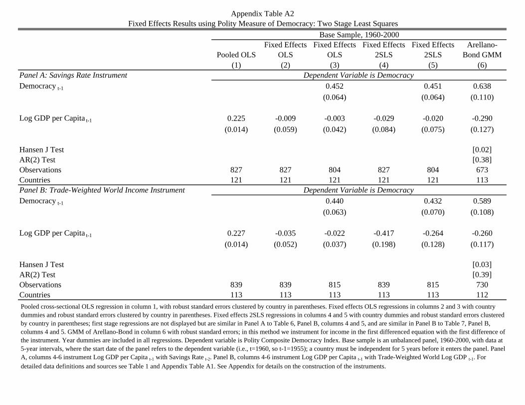
Pooled OLSFixed Effects

OLSFixed Effects

OLSFixed Effects

2SLSFixed Effects

2SLSArellano-

Bond GMM(1) (2) (3) (4) (5) (6)

Panel A: Savings Rate InstrumentDemocracy t-1 0.452 0.451 0.638

(0.064) (0.064) (0.110)

Log GDP per Capita t-1 0.225 -0.009 -0.003 -0.029 -0.020 -0.290(0.014) (0.059) (0.042) (0.084) (0.075) (0.127)

Hansen J Test [0.02]AR(2) Test [0.38]Observations 827 827 804 827 804 673Countries 121 121 121 121 121 113Panel B: Trade-Weighted World Income InstrumentDemocracy t-1 0.440 0.432 0.589

(0.063) (0.070) (0.108)

Log GDP per Capita t-1 0.227 -0.035 -0.022 -0.417 -0.264 -0.260(0.014) (0.052) (0.037) (0.198) (0.128) (0.117)

Hansen J Test [0.03]AR(2) Test [0.39]Observations 839 839 815 839 815 730Countries 113 113 113 113 113 112

Appendix Table A2Fixed Effects Results using Polity Measure of Democracy: Two Stage Least Squares

Dependent Variable is Democracy

Dependent Variable is Democracy

Base Sample, 1960-2000

Pooled cross-sectional OLS regression in column 1, with robust standard errors clustered by country in parentheses. Fixed effects OLS regressions in columns 2 and 3 with country dummies and robust standard errors clustered by country in parentheses. Fixed effects 2SLS regressions in columns 4 and 5 with country dummies and robust standard errors clustered by country in parentheses; first stage regressions are not displayed but are similar in Panel A to Table 6, Panel B, columns 4 and 5, and are similar in Panel B to Table 7, Panel B, columns 4 and 5. GMM of Arellano-Bond in column 6 with robust standard errors; in this method we instrument for income in the first differenced equation with the first difference of the instrument. Year dummies are included in all regressions. Dependent variable is Polity Composite Democracy Index. Base sample is an unbalanced panel, 1960-2000, with data at 5-year intervals, where the start date of the panel refers to the dependent variable (i.e., t=1960, so t-1=1955); a country must be independent for 5 years before it enters the panel. Panel A, columns 4-6 instrument Log GDP per Capita t-1 with Savings Rate t-2. Panel B, columns 4-6 instrument Log GDP per Capita t-1 with Trade-Weighted World Log GDP t-1. For detailed data definitions and sources see Table 1 and Appendix Table A1. See Appendix for details on the construction of the instruments.

Balanced Panel 1970-

2000Pooled OLS Fixed Effects

(1) (2) (3) (4) (5) (6) (7) (8)

Democracy t-1 0.723 0.354 0.711 0.720 0.643 0.622 0.637 0.549(0.047) (0.078) (0.050) (0.048) (0.054) (0.057) (0.053) (0.083)

Log GDP per Capita t-1 0.043 -0.056 0.032 0.032 0.015 0.009 0.004 -0.010(0.014) (0.060) (0.017) (0.014) (0.012) (0.018) (0.013) (0.020)

Constraint on the Executive at Independence 0.131 0.153 0.137 0.169(0.037) (0.037) (0.036) (0.050)

Independence Year/100 -0.083 -0.087 -0.081 -0.119(0.016) (0.018) (0.016) (0.029)

Log Population Density in 1500 -0.010 -0.009 -0.011 -0.019(0.006) (0.008) (0.007) (0.010)

Log Settler Mortality -0.019 -0.001(0.010) (0.010)

Observations 514 514 462 514 514 462 514 273Countries 80 80 68 80 80 68 80 39R-squared 0.68 0.76 0.70 0.69 0.70 0.71 0.70 0.71

Appendix Table A3Effect of Historical Factors on Democracy: Former Colonies, using Polity Measure of Democracy

Dependent Variable is Democracy

Former European Colonies

Pooled OLSUnbalanced Panel, 1960-2000

Pooled cross-sectional OLS in columns 1 and 3-8, with robust standard errors clustered by country in parentheses. Fixed effects OLS regressions in column 2, with country dummies and robust standard errors clustered by country in parentheses. Year dummies are included in all regressions. Dependent variable is Polity Composite Democracy Index. Data are at 5-year intervals, for former European colonies. Columns 1-7 are an unbalanced panel in levels where the start date of the panel refers to the dependent variable (i.e., t=1960, so t-1=1955); a country must be independent for 10 years before it enters the panel. Column 8 is a balanced panel from 1970 to 2000; a country must be independent by 1960 to enter the panel and first lagged value is 1965. In all columns, data represents all available values in the former colonies sample for which Constraint on the Executive at Independence, Independence Year, and Log Population Density in 1500 are available. For detailed data definitions and sources see Table 1 and Appendix Table A1.

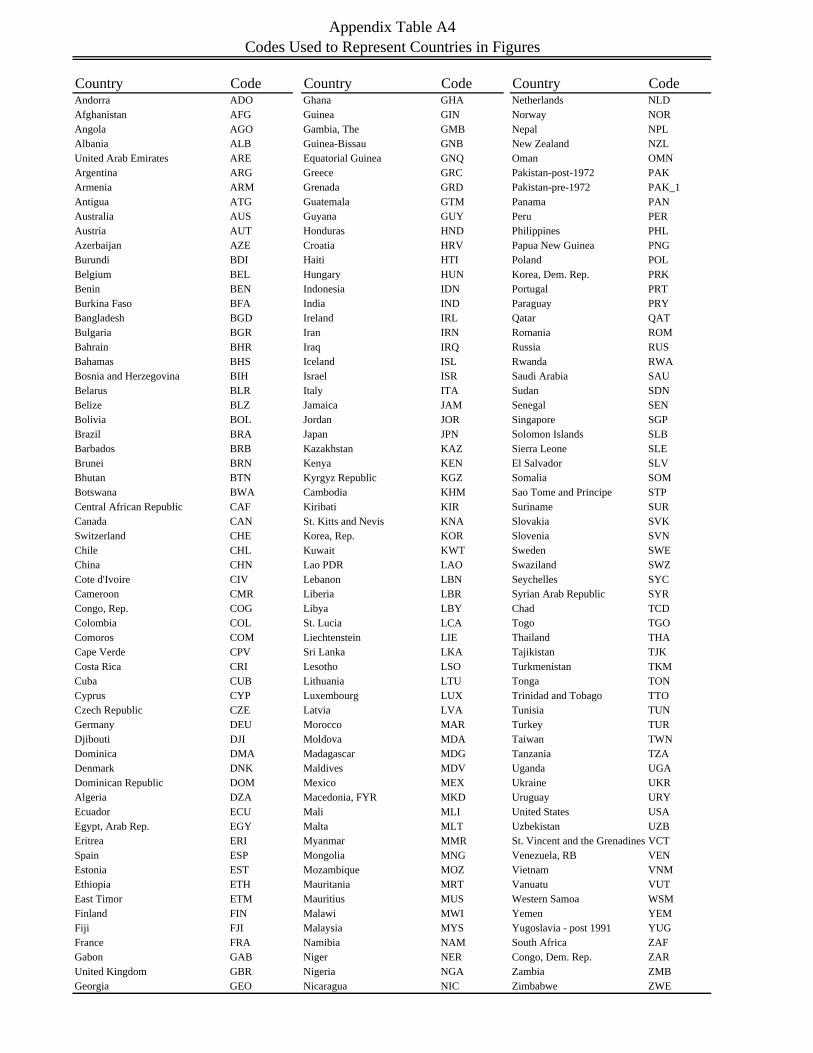
Country Code Country Code Country CodeAndorra ADO Ghana GHA Netherlands NLDAfghanistan AFG Guinea GIN Norway NORAngola AGO Gambia, The GMB Nepal NPLAlbania ALB Guinea-Bissau GNB New Zealand NZLUnited Arab Emirates ARE Equatorial Guinea GNQ Oman OMNArgentina ARG Greece GRC Pakistan-post-1972 PAKArmenia ARM Grenada GRD Pakistan-pre-1972 PAK_1Antigua ATG Guatemala GTM Panama PANAustralia AUS Guyana GUY Peru PERAustria AUT Honduras HND Philippines PHLAzerbaijan AZE Croatia HRV Papua New Guinea PNGBurundi BDI Haiti HTI Poland POLBelgium BEL Hungary HUN Korea, Dem. Rep. PRKBenin BEN Indonesia IDN Portugal PRTBurkina Faso BFA India IND Paraguay PRYBangladesh BGD Ireland IRL Qatar QATBulgaria BGR Iran IRN Romania ROMBahrain BHR Iraq IRQ Russia RUSBahamas BHS Iceland ISL Rwanda RWABosnia and Herzegovina BIH Israel ISR Saudi Arabia SAUBelarus BLR Italy ITA Sudan SDNBelize BLZ Jamaica JAM Senegal SENBolivia BOL Jordan JOR Singapore SGPBrazil BRA Japan JPN Solomon Islands SLBBarbados BRB Kazakhstan KAZ Sierra Leone SLEBrunei BRN Kenya KEN El Salvador SLVBhutan BTN Kyrgyz Republic KGZ Somalia SOMBotswana BWA Cambodia KHM Sao Tome and Principe STPCentral African Republic CAF Kiribati KIR Suriname SURCanada CAN St. Kitts and Nevis KNA Slovakia SVKSwitzerland CHE Korea, Rep. KOR Slovenia SVNChile CHL Kuwait KWT Sweden SWEChina CHN Lao PDR LAO Swaziland SWZCote d'Ivoire CIV Lebanon LBN Seychelles SYCCameroon CMR Liberia LBR Syrian Arab Republic SYRCongo, Rep. COG Libya LBY Chad TCDColombia COL St. Lucia LCA Togo TGOComoros COM Liechtenstein LIE Thailand THACape Verde CPV Sri Lanka LKA Tajikistan TJKCosta Rica CRI Lesotho LSO Turkmenistan TKMCuba CUB Lithuania LTU Tonga TONCyprus CYP Luxembourg LUX Trinidad and Tobago TTOCzech Republic CZE Latvia LVA Tunisia TUNGermany DEU Morocco MAR Turkey TURDjibouti DJI Moldova MDA Taiwan TWNDominica DMA Madagascar MDG Tanzania TZADenmark DNK Maldives MDV Uganda UGADominican Republic DOM Mexico MEX Ukraine UKRAlgeria DZA Macedonia, FYR MKD Uruguay URYEcuador ECU Mali MLI United States USAEgypt, Arab Rep. EGY Malta MLT Uzbekistan UZBEritrea ERI Myanmar MMR St. Vincent and the Grenadines VCTSpain ESP Mongolia MNG Venezuela, RB VENEstonia EST Mozambique MOZ Vietnam VNMEthiopia ETH Mauritania MRT Vanuatu VUTEast Timor ETM Mauritius MUS Western Samoa WSMFinland FIN Malawi MWI Yemen YEMFiji FJI Malaysia MYS Yugoslavia - post 1991 YUGFrance FRA Namibia NAM South Africa ZAFGabon GAB Niger NER Congo, Dem. Rep. ZARUnited Kingdom GBR Nigeria NGA Zambia ZMBGeorgia GEO Nicaragua NIC Zimbabwe ZWE

Codes Used to Represent Countries in FiguresAppendix Table A4

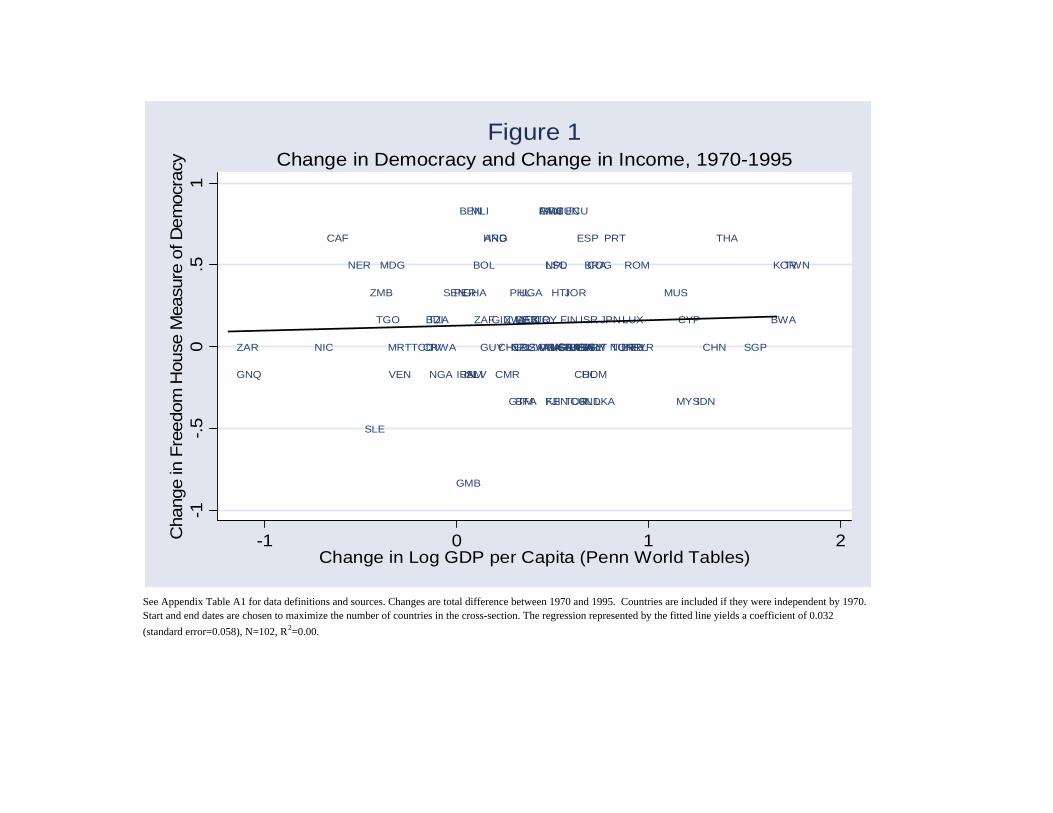
See Appendix Table A1 for data definitions and sources. Changes are total difference between 1970 and 1995. Countries are included if they were independent by 1970. Start and end dates are chosen to maximize the number of countries in the cross-section. The regression represented by the fitted line yields a coefficient of 0.032 (standard error=0.058), N=102, R2=0.00.

ARG

AUS AUT

BDI

BEL

BEN

BFA

BOL BRA

BRB

BWA

CAF

CANCHE

CHL

CHNCIV

CMR

COG

COL

CRI

CYP

DNK

DOM

DZA

ECU

EGY

ESP

FIN

FJI

FRA

GAB

GBR

GHA

GIN

GMB

GNQ

GRC

GTM

GUY

HND

HTI

HUN

IDNIND

IRL

IRN

ISL

ISR

ITA

JAM

JOR

JPN

KEN

KOR

LKA

LSO

LUX

MAR

MDG

MEX

MLI

MRT

MUS

MWI

MYS

NER

NGA

NIC NLD NOR

NPL

NZL

PAN

PER PHL

PRT

PRY

ROM

RWA

SEN

SGP

SLE

SLV

SWE SYRTCD

TGO

THA

TTO

TUN

TUR

TWN

TZA

UGA

URY

USA

VEN

ZAF

ZAR

ZMB

ZWE

-1-.5

0.5

1C

hang

e in

Fre

edom

Hou

se M

easu

re o

f Dem

ocra

cy

-1 0 1 2Change in Log GDP per Capita (Penn World Tables)

Change in Democracy and Change in Income, 1970-1995Figure 1

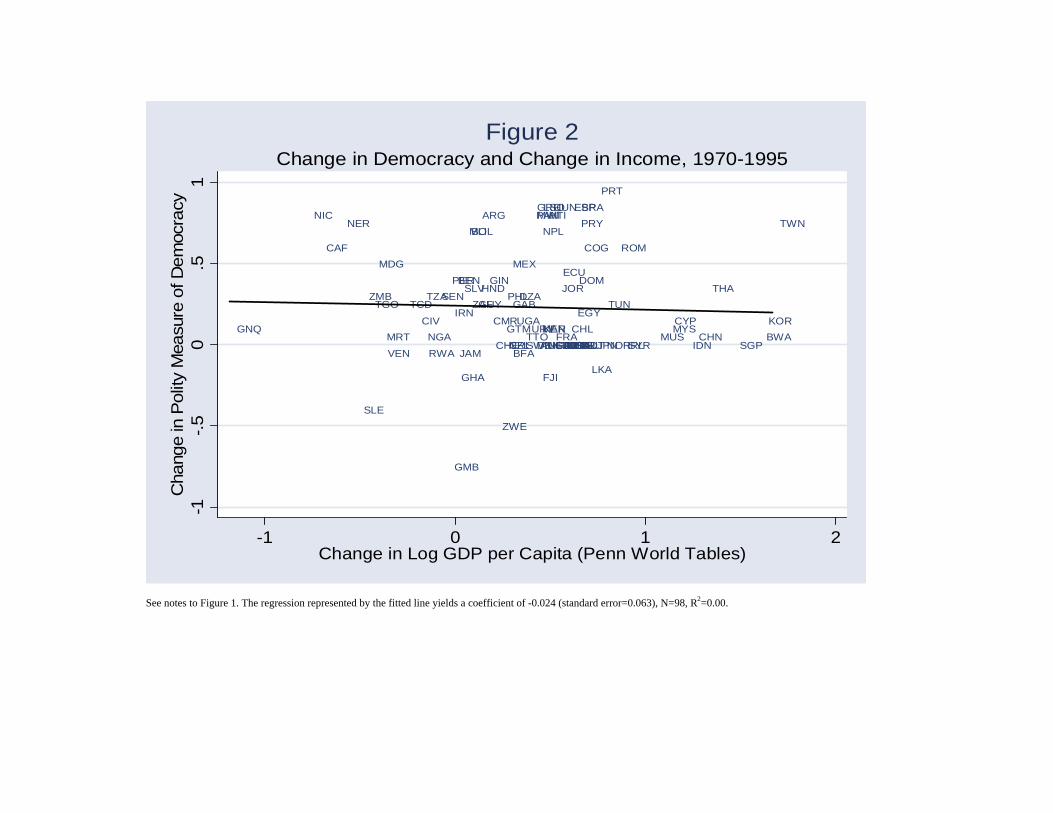
See notes to Figure 1. The regression represented by the fitted line yields a coefficient of -0.024 (standard error=0.063), N=98, R2=0.00.

ARG

AUS AUTBEL

BEN

BFA

BOL

BRA

BWA

CAF

CANCHECHL

CHNCIV CMR

COG

COLCRI

CYP

DNK

DOMDZA

ECU

EGY

ESP

FIN

FJI

FRA

GAB

GBR

GHA

GIN

GMB

GNQ

GRC

GTM

GUYHND

HTIHUN

IDNIND IRL

IRN

ISLISRITAJAM

JOR

JPNKEN

KOR

LKA

LSO

MAR

MDG MEX

MLI

MRT MUS

MWI

MYS

NER

NGA

NIC

NLD NOR

NPL

NZL

PAN

PERPHL

PRT

PRY

ROM

RWA

SEN

SGP

SLE

SLV

SWE SYR

TCDTGOTHA

TTO

TUN

TUR

TWN

TZA

UGAURY

USAVEN

ZAFZMB

ZWE

-1-.5

0.5

1C

hang

e in

Pol

ity M

easu

re o

f Dem

ocra

cy

-1 0 1 2Change in Log GDP per Capita (Penn World Tables)

Change in Democracy and Change in Income, 1970-1995Figure 2

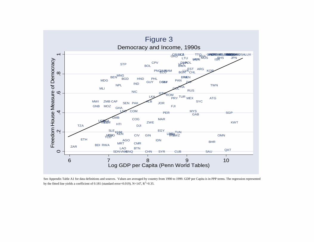
See Appendix Table A1 for data definitions and sources. Values are averaged by country from 1990 to 1999. GDP per Capita is in PPP terms. The regression represented by the fitted line yields a coefficient of 0.181 (standard error=0.019), N=147, R2=0.35.

AGO

ALB

ARG

ATG

AUSAUT

BDI

BEL

BEN

BFA

BGD

BGR

BHR

BHSBLZ

BOL

BRA

BRB

BTN

BWA

CAF

CANCHE

CHL

CHN

CIV

CMR

COG

COL

COM

CPV

CRI

CUB

CYP DEU

DJI

DMA

DNK

DOM

DZA

ECU

EGY

ESP

EST

ETH

FIN

FJI

FRA

GAB

GBR

GHA

GIN

GMB

GNB

GNQ

GRCGRD

GTM

GUYHND

HTI

HUN

IDN

IND

IRL

IRN

ISLISR

ITA

JAM

JOR

JPN

KENKHM

KNA

KOR

KWT

LAO

LBN

LCA

LKA

LSO

LTULUX

LVA

MAR

MDG

MEX

MLI

MLT

MNG

MOZ

MRT

MUS

MWI

MYS

NAM

NER

NGA

NIC

NLDNOR

NPL

NZL

OMN

PAK

PAN

PER

PHL

PNG

POL

PRT

PRY

QAT

ROMRUS

RWA

SAUSDN

SEN

SGP

SLE

SLV

STP

SWE

SWZ

SYC

SYR

TCDTGO

THA

TTO

TUN

TUR

TWN

TZAUGA

URYUSA

VCT

VEN

VNM

YEM

ZAF

ZAR

ZMB

ZWE

0.2

.4.6

.81

Free

dom

Hou

se M

easu

re o

f Dem

ocra

cy

6 7 8 9 10Log GDP per Capita (Penn World Tables)

Democracy and Income, 1990sFigure 3

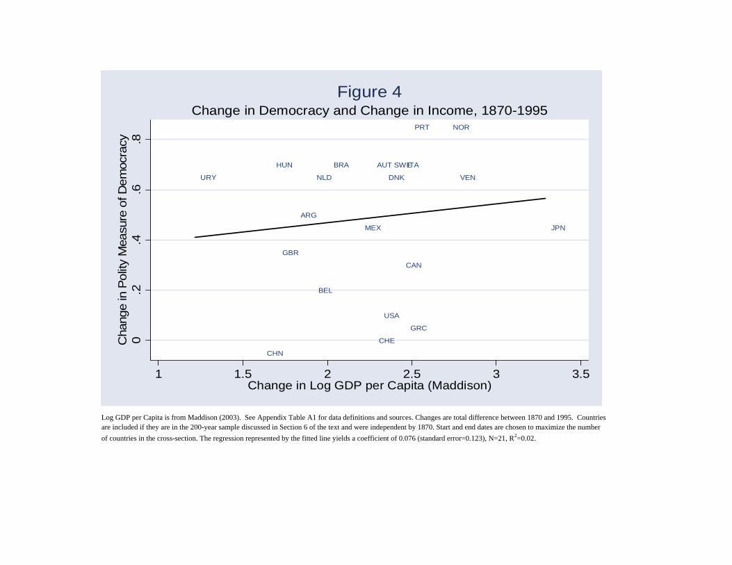
Log GDP per Capita is from Maddison (2003). See Appendix Table A1 for data definitions and sources. Changes are total difference between 1870 and 1995. Countries are included if they are in the 200-year sample discussed in Section 6 of the text and were independent by 1870. Start and end dates are chosen to maximize the number of countries in the cross-section. The regression represented by the fitted line yields a coefficient of 0.076 (standard error=0.123), N=21, R2=0.02.

ARG

AUT

BEL

BRA

CAN

CHE

CHN

DNK

GBR

GRC

HUN ITA

JPNMEX

NLD

NORPRT

SWE

URY

USA

VEN

0.2

.4.6

.8C

hang

e in

Pol

ity M

easu

re o

f Dem

ocra

cy

1 1.5 2 2.5 3 3.5Change in Log GDP per Capita (Maddison)

Change in Democracy and Change in Income, 1870-1995Figure 4

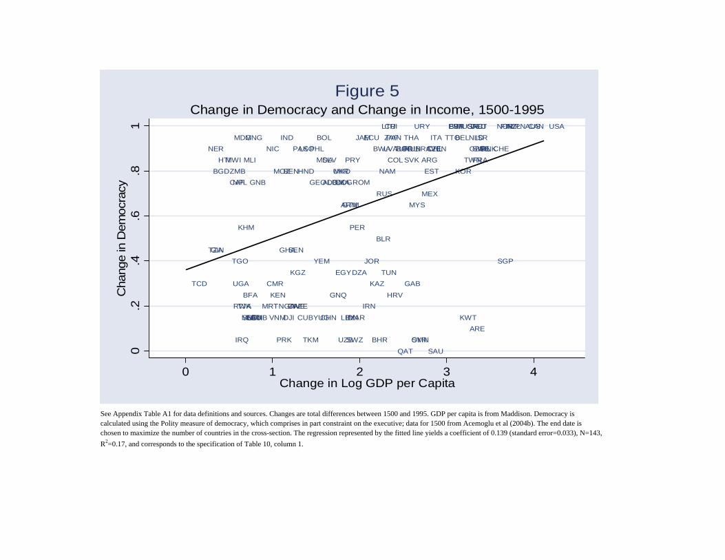
See Appendix Table A1 for data definitions and sources. Changes are total differences between 1500 and 1995. GDP per capita is from Maddison. Democracy is calculated using the Polity measure of democracy, which comprises in part constraint on the executive; data for 1500 from Acemoglu et al (2004b). The end date is chosen to maximize the number of countries in the cross-section. The regression represented by the fitted line yields a coefficient of 0.139 (standard error=0.033), N=143, R2=0.17, and corresponds to the specification of Table 10, column 1.

ALB

ARE

ARG

ARM

AUSAUT

AZE

BEL

BEN

BFA

BGD

BGR

BHR

BLR

BOLBRABWA

CAF

CAN

CHECHL

CHNCIV

CMR

COG

COL

CRI

CUB

CZE

DEU

DJI

DNK

DOM

DZA

ECU

EGY

ESP

EST

FIN

FRA

GAB

GBR

GEO

GHAGIN

GMB

GNB

GNQ

GRC

GTM

HND

HRV

HTIHUN

IDN

INDIRL

IRN

IRQ

ISRITAJAM

JOR

JPN

KAZKEN

KGZ

KHM

KOR

KWTLAO LBY

LKA

LSO

LTU

LVA

MAR

MDA

MDG

MEX

MKDMLI

MMR

MNG

MOZ

MRT

MUS

MWI

MYS

NAM

NER

NGA

NICNLD

NOR

NPL

NZL

OMN

PAKPAN

PER

PHL POL

PRK

PRT

PRY

QAT

ROMRUS

RWA

SAU

SDN

SENSGP

SLE

SLV SVK

SVN

SWE

SWZ SYR

TCD

TGO

THA

TJK

TKM

TTO

TUN

TURTWN

TZA

UGA

UKR

URY USA

UZB

VEN

VNM

YEM

YUG

ZAF

ZMB

ZWE

0.2

.4.6

.81

Cha

nge

in D

emoc

racy

0 1 2 3 4Change in Log GDP per Capita

Change in Democracy and Change in Income, 1500-1995Figure 5

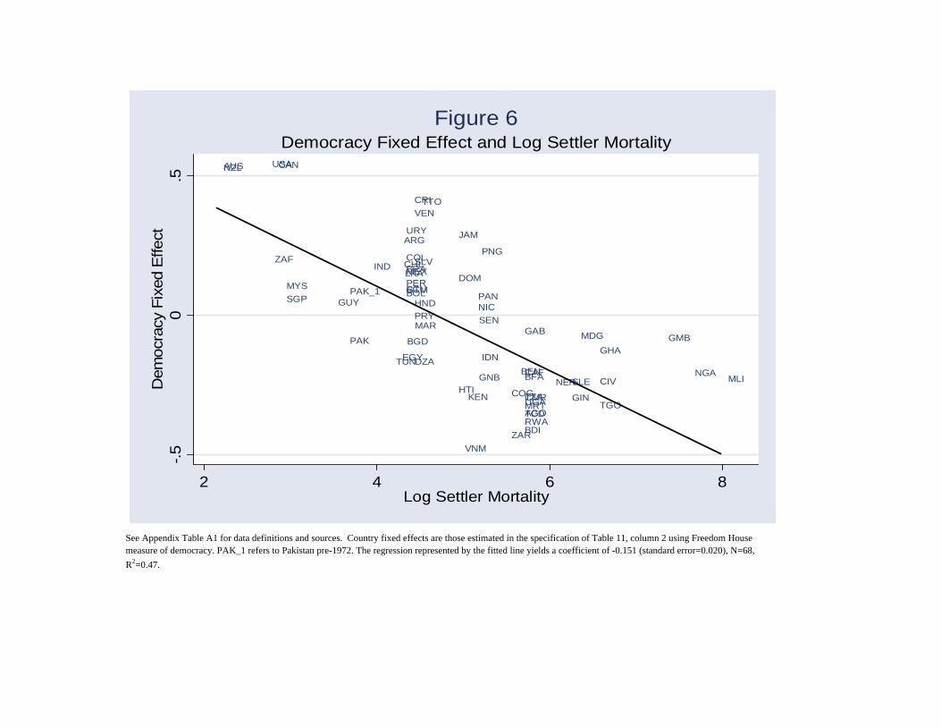
See Appendix Table A1 for data definitions and sources. Country fixed effects are those estimated in the specification of Table 11, column 2 using Freedom House measure of democracy. PAK_1 refers to Pakistan pre-1972. The regression represented by the fitted line yields a coefficient of -0.151 (standard error=0.020), N=68, R2=0.47.

AGO

ARG

AUS

BDI

BENBFA

BGD

BOL

BRA

CAF

CAN

CHL

CIV

CMRCOG

COL

CRI

DOM

DZA

ECU

EGY

GAB

GHA

GIN

GMB

GNB

GTMGUY HND

HTI

IDN

IND

JAM

KEN

LKA

MARMDG

MEX

MLI

MRT

MYS

NERNGA

NIC

NZL

PAK

PAK_1 PANPER

PNG

PRY

RWA

SEN

SGP

SLE

SLV

TCDTGO

TTO

TUN

TZAUGA

URY

USA

VEN

VNM

ZAF

ZAR

-.50

.5D

emoc

racy

Fix

ed E

ffect

2 4 6 8Log Settler Mortality

Democracy Fixed Effect and Log Settler MortalityFigure 6

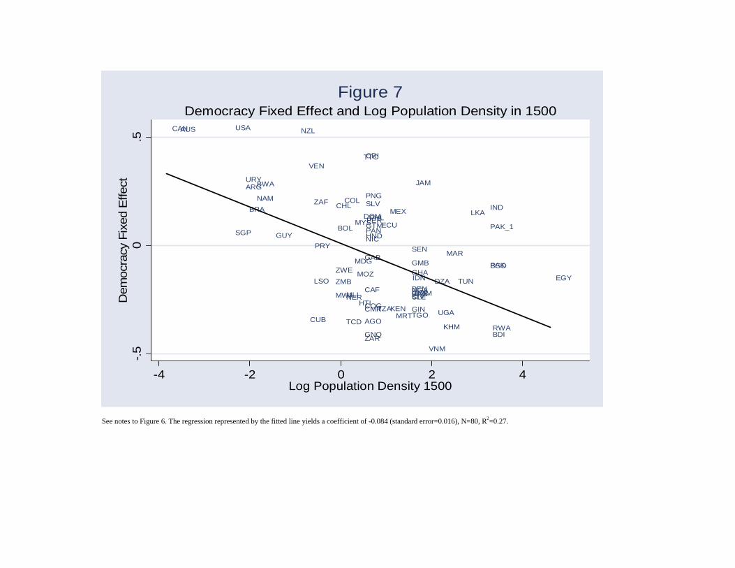
See notes to Figure 6. The regression represented by the fitted line yields a coefficient of -0.084 (standard error=0.016), N=80, R2=0.27.

AGO

ARG

AUS

BDI

BENBFA

BGD

BOL

BRA

BWA

CAF

CAN

CHL

CIV

CMRCOG

COL

COM

CRI

CUB

DOM

DZA

ECU

EGY

GAB

GHA

GIN

GMB

GNB

GNQ

GTMGUY HND

HTI

IDN

IND

JAM

KEN

KHM

LKA

LSO

MARMDG

MEX

MLI

MOZ

MRT

MWI

MYS

NAM

NERNGA

NIC

NZL

PAK

PAK_1PANPERPHL

PNG

PRY

RWA

SEN

SGP

SLE

SLV

TCDTGO

TTO

TUN

TZA UGA

URY

USA

VEN

VNM

ZAF

ZAR

ZMBZWE

-.50

.5D

emoc

racy

Fix

ed E

ffect

-4 -2 0 2 4Log Population Density 1500

Democracy Fixed Effect and Log Population Density in 1500Figure 7

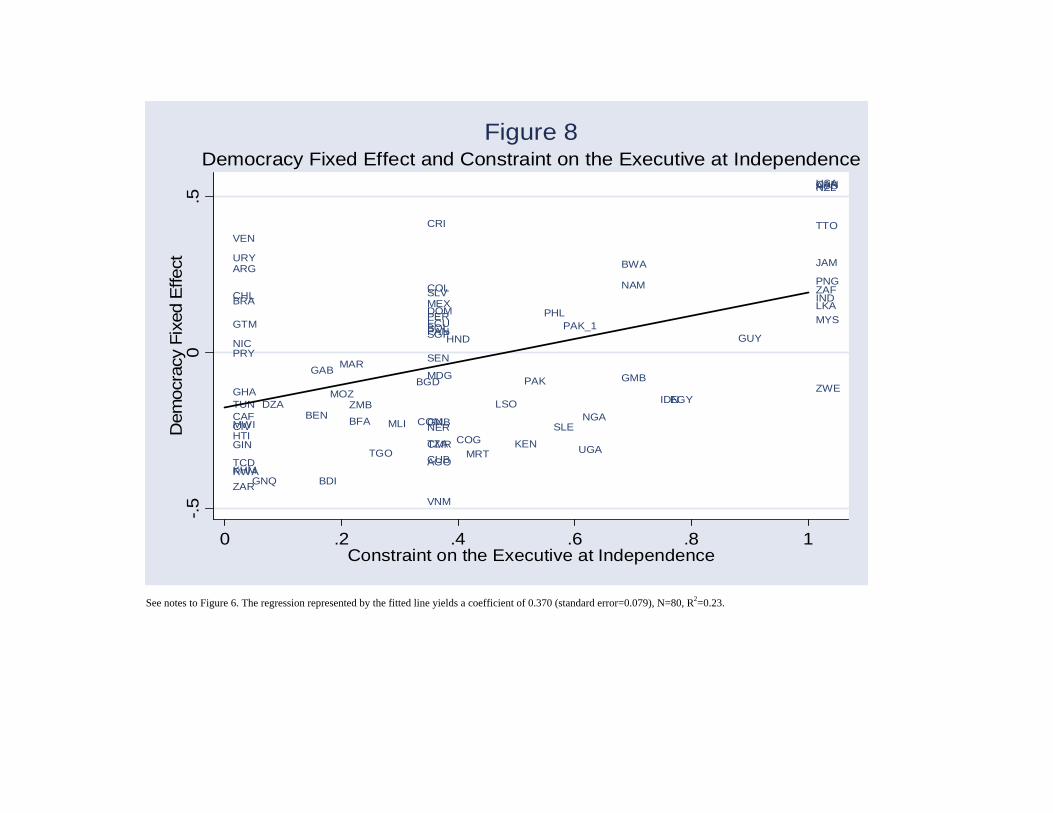
See notes to Figure 6. The regression represented by the fitted line yields a coefficient of 0.370 (standard error=0.079), N=80, R2=0.23.

AGO

ARG

AUS

BDI

BEN BFA

BGD

BOL

BRA

BWA

CAF

CAN

CHL

CIV

CMR COG

COL

COM

CRI

CUB

DOM

DZA

ECU

EGY

GAB

GHA

GIN

GMB

GNB

GNQ

GTMGUYHND

HTI

IDN

IND

JAM

KEN

KHM

LKA

LSO

MARMDG

MEX

MLI

MOZ

MRT

MWI

MYS

NAM

NERNGA

NIC

NZL

PAK

PAK_1PANPER PHL

PNG

PRY

RWA

SEN

SGP

SLE

SLV

TCDTGO

TTO

TUN

TZA UGA

URY

USA

VEN

VNM

ZAF

ZAR

ZMBZWE

-.50

.5D

emoc

racy

Fix

ed E

ffect

0 .2 .4 .6 .8 1Constraint on the Executive at Independence

Democracy Fixed Effect and Constraint on the Executive at IndependenceFigure 8

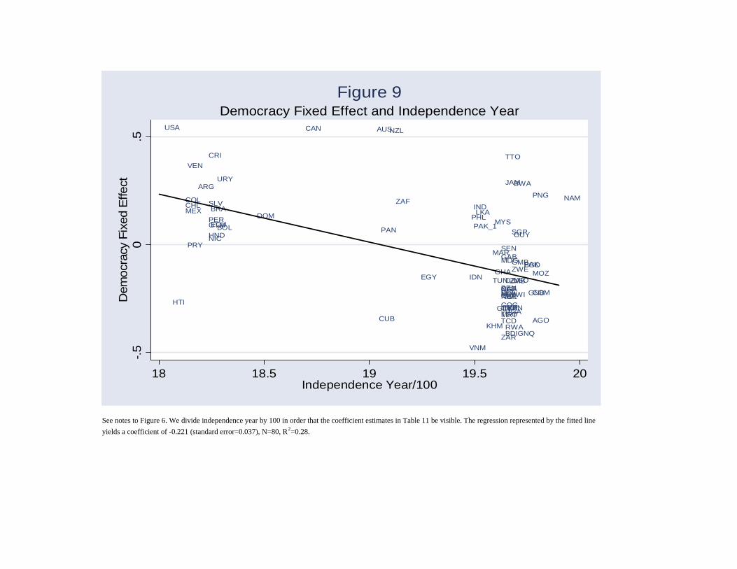
See notes to Figure 6. We divide independence year by 100 in order that the coefficient estimates in Table 11 be visible. The regression represented by the fitted line yields a coefficient of -0.221 (standard error=0.037), N=80, R2=0.28.

AGO

ARG

AUS

BDI

BENBFA

BGD

BOL

BRA

BWA

CAF

CAN

CHL

CIV

CMRCOG

COL

COM

CRI

CUB

DOM

DZA

ECU

EGY

GAB

GHA

GIN

GMB

GNB

GNQ

GTMGUYHND

HTI

IDN

IND

JAM

KEN

KHM

LKA

LSO

MARMDG

MEX

MLI

MOZ

MRT

MWI

MYS

NAM

NERNGA

NIC

NZL

PAK

PAK_1PANPER PHL

PNG

PRY

RWA

SEN

SGP

SLE

SLV

TCDTGO

TTO

TUN

TZAUGA

URY

USA

VEN

VNM

ZAF

ZAR

ZMBZWE

-.50

.5D

emoc

racy

Fix

ed E

ffect

18 18.5 19 19.5 20Independence Year/100

Democracy Fixed Effect and Independence YearFigure 9

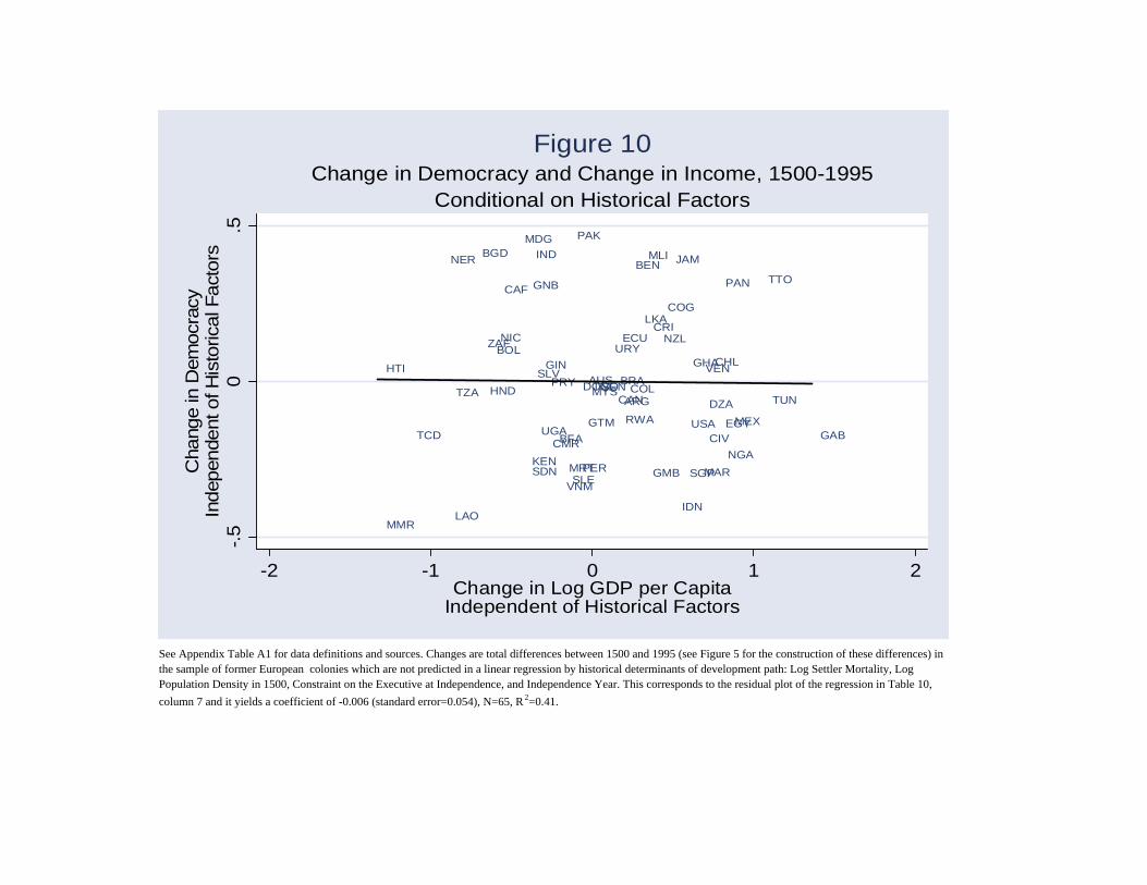
See Appendix Table A1 for data definitions and sources. Changes are total differences between 1500 and 1995 (see Figure 5 for the construction of these differences) in the sample of former European colonies which are not predicted in a linear regression by historical determinants of development path: Log Settler Mortality, Log Population Density in 1500, Constraint on the Executive at Independence, and Independence Year. This corresponds to the residual plot of the regression in Table 10, column 7 and it yields a coefficient of -0.006 (standard error=0.054), N=65, R 2=0.41.

ARG

AUS

BEN

BFA

BGD

BOL

BRA

CAF

CAN

CHL

CIVCMR

COG

COL

CRI

DOMDZA

ECU

EGYGAB

GHAGIN

GMB

GNB

GTM

HND

HTI

IDN

IND JAM

KEN

LAO

LKA

MAR

MDG

MEX

MLI

MMR

MRT

MYS

NER

NGA

NIC NZL

PAK

PAN

PER

PRY

RWA

SDN

SEN

SGPSLE

SLV

TCD

TGO

TTO

TUNTZA

UGA

URY

USA

VEN

VNM

ZAF

-.50

.5

Cha

nge

in D

emoc

racy

Inde

pend

ent o

f His

toric

al F

acto

rs

-2 -1 0 1 2Change in Log GDP per Capita

Independent of Historical Factors

Conditional on Historical FactorsChange in Democracy and Change in Income, 1500-1995

Figure 10