NBER WORKING PAPER SERIES

EXPENDITURE SWITCHING VS. REAL EXCHANGE RATESTABILIZATION: COMPETING OBJECTIVES FOR

EXCHANGE RATE POLICY

Michael B. DevereuxCharles Engel

Working Paper 12215http://www.nber.org/papers/w12215

NATIONAL BUREAU OF ECONOMIC RESEARCH1050 Massachusetts Avenue

Cambridge, MA 02138May 2006

The authors thank Martin Eichenbaum and an anonymous referee for very helpful comments. Theyacknowledge support from the Hong Kong Institute for Monetary Research, where work on this projectbegan. Engel also acknowledges assistance from the National Science Foundation through a grant toUniversity of Wisconsin. Devereux thanks the Social Sciences and Humanities Research Council of Canada,the Bank of Canada, and the Royal Bank of Canada for financial assistance. The views expressed herein arethose of the author(s) and do not necessarily reflect the views of the National Bureau of Economic Research.

©2006 by Michael B. Devereux and Charles Engel. All rights reserved. Short sections of text, not to exceedtwo paragraphs, may be quoted without explicit permission provided that full credit, including © notice, isgiven to the source.

Expenditure Switching vs. Real Exchange Rate Stabilization: Competing Objectives forExchange Rate PolicyMichael B. Devereux and Charles EngelNBER Working Paper No. 12215May 2006JEL No. F3, F4, E5

ABSTRACT

This paper develops a view of exchange rate policy as a trade-off between the desire to smoothfluctuations in real exchange rates so as to reduce distortions in consumption allocations, and theneed to allow flexibility in the nominal exchange rate so as to facilitate terms of trade adjustment.We show that optimal nominal exchange rate volatility will reflect these competing objectives. Thekey determinants of how much the exchange rate should respond to shocks will depend on the extentand source of price stickiness, the elasticity of substitution between home and foreign goods, and theamount of home bias in production. Quantitatively, we find the optimal exchange rate volatilityshould be significantly less than would be inferred based solely on terms of trade considerations.Moreover, we find that the relationship between price stickiness and optimal exchange rate volatilitymay be non-monotonic.

Charles M. EngelDepartment of EconomicsUniversity of Wisconsin1180 Observatory DriveMadison, WI 53706-1393and NBERcengel@ssc.wisc.edu

This paper develops a novel view of exchange rate policy as a trade-off between the desire to

smooth fluctuations in real exchange rates in order to achieve smaller cross-country deviations in

consumer prices on the one hand, and the need to allow flexibility in the nominal exchange rate so as to

facilitate terms of trade adjustment on the other hand.

There is a substantial body of empirical evidence establishing that the link between movements in

exchange rates and changes in national consumer prices is weak.1 One explanation for this weak link is

that prices of all goods are sticky in local currencies (LCP, or local currency pricing), and do not respond

to movements in the exchange rate. In this case, nominal exchange rate fluctuations lead to inefficient

movements in real exchange rates because they alter relative prices of identical or similar goods across

countries. From this perspective, it is desirable to avoid movements in exchange rates because they lead

to differences in prices across countries for goods that have similar resource costs.2

But there is separate evidence that relative traded goods prices are linked to movements in

exchange rates. Obstfeld and Rogoff (2000) show that exchange rates are highly correlated with the

terms of trade, measured as the relative price of imports to exports. This suggests that exported goods

tend to have prices set in the producer’s currency (PCP, or producer’s currency pricing), and a

depreciation raises the relative price of foreign to home export goods. In this case, the exchange rate may

play a role in facilitating relative price adjustment in face of country specific shocks when nominal prices

of traded goods are slow to adjust to the shocks.

We present an analysis of exchange rate policy when there is a conflict between the objectives of

stabilizing consumption-based real exchange rates and allowing terms of trade adjustment. We build a

model consistent with both the evidence of weak exchange rate pass-through to consumer goods prices

and high pass-through to imported goods prices. In the model, imports and exports are intermediate

goods. The law of one price holds for these traded products, so nominal price stickiness of these goods is

of the PCP variety. Intermediate goods are used to produce final consumer goods, whose prices are sticky

in the consumers’ currency. Consistent with the evidence, consumer prices are unresponsive to nominal

exchange rate changes. In general, optimal exchange rate movements in this setting do not deliver full

terms of trade adjustment. There is a trade-off. Nominal exchange rate movement changes the terms of

trade in the desired direction when there is a real shock, as the literature has suggested, but mimicking the

optimal terms of trade change may imply undesirable changes in the consumption-based real exchange

rate.

In our model, the optimal real exchange rate is constant only when the production functions for

the final consumption good in the home and foreign country are identical and use only traded inputs. If 1 See Engel (1993, 1999), Rogers and Jenkins (1996), Engel and Rogers (1996, 2001), Obstfeld and Taylor (1997), and Parsley and Wei (2001, 2003). Mussa’s (1986) classic paper stimulated much of this research. 2 Devereux and Engel (2003) find that if exporters set prices according to LCP, a fixed exchange rate regime is the optimal monetary policy. Similar results are found in Corsetti and Pesenti (2002).

1

we consider that special case, then under LCP for final goods, nominal exchange rate changes induce

movements in real exchange rates that lead to inefficient consumption allocations. Stabilization of the

consumption real exchange rate is a legitimate goal of exchange-rate policy, but it conflicts with the

objective of achieving terms of trade adjustment. Moreover, when the production functions are not

identical (e.g., exhibiting home bias in the use of traded inputs), or when non-traded inputs are used in

production, the optimal real exchange rate is not constant. It is nonetheless true that the optimal policy

stabilizes real exchange rates relative to the terms of trade.3

Evidence that the law of one price holds relatively well for traded intermediate goods is

consistent with PCP, but is also consistent with nominal price flexibility for these goods. The evidence is

not refined enough to distinguish between the two possibilities. Markets for intermediate inputs are not

the standard “customer” markets to which models of nominal price stickiness are typically applied. To

the extent that traded intermediate prices are flexible, exchange rate adjustment is not needed to adjust the

terms of trade because the nominal prices themselves can adjust.

Additionally, in the short run, domestically produced products might not be easily substituted for

imported intermediate goods. If the substitutability of imported intermediates with domestic goods and

services is low, the expenditure-switching role of exchange rates may be secondary. It is the short-run

elasticity of substitution that is relevant for exchange-rate policy: when nominal prices have had time to

adjust, the real effects of nominal exchange rate changes dissipate. It is well known that the short-run

elasticity of substitution for imports is quite low. Even if prices are sticky and set according to PCP, so

that nominal exchange rate movements do change the relative price of imported goods, there will be little

expenditure switching when substitutability is low.

We first present a series of special cases where monetary policy can achieve a first-best outcome

– stabilizing the consumption real exchange rate as well as supporting efficient terms of trade adjustment.

In our first specification, nominal prices of consumer goods are set in advance of the realization of

shocks, while prices of intermediate goods are taken to be perfectly flexible. We find that under an

optimal monetary policy, the nominal and real exchange rate has a lower variance than the optimal terms

of trade movements. Under some parameterizations, an optimal monetary policy keeps the exchange rate

constant. In this case, the fully optimal consumption allocations can be attained. The prices of traded

intermediates adjust freely in response to shocks, so the role of monetary policy effectively is to achieve

the desired real exchange rate response.

We then reverse the assumptions on stickiness – final goods prices are flexible, but intermediate

goods prices are set in advance in the producer’s currency. Here we find that optimal exchange rate

policy is aimed purely at achieving the desired terms of trade adjustment, since flexible final goods prices

3 Empirically, Engel (1999) has found that variation in the relative price of pure non-traded goods can account for very little of the short-run real exchange rate movements in advanced countries.

2

will ensure a stable real exchange rate. This specification is, of course, at odds with the evidence of non-

responsiveness of consumer prices to exchange rate movements.

We also solve a version of the model in which the home and foreign inputs must be combined in

fixed proportions. We illustrate an example where fixed exchange rates are optimal even when both

intermediate and final goods prices are fixed in advance (with PCP for intermediates and LCP for final

goods.) There is no expenditure-switching role for exchange rates when there is no substitutability

between imports and domestically-produced goods.

In general, however, monetary policy will not be able to attain simultaneously fully optimal

consumption allocations as well as optimal terms of trade adjustment. In particular, when both final

goods prices and intermediate goods prices are partially sticky, this will be the case. We go on to present

a quantitative analysis of the more general case where there is a real trade-off between these goals. Our

analysis finds that when consumer price indices are unresponsive to exchange rate changes, an optimal

monetary policy will limit exchange rate volatility substantially relative to that required to achieve terms

of trade volatility in a frictionless economy – even when most or all intermediate goods prices are sticky

in nominal terms.

In addition, we show that the relationship between exchange rate volatility and price stickiness

may not be monotonic. While intuitively one would anticipate that reducing the flexibility of

intermediate prices would increase the desirability of exchange rate adjustment, this relationship does not

necessarily hold when the elasticity of substitution between home and imported intermediates is relatively

low. We show that reducing the flexibility of intermediate goods prices will first increase desired

exchange rate volatility. But after a certain point, as a greater share of intermediate goods prices are

sticky, it becomes desirable to reduce exchange rate volatility.

The paper is organized as follows. Section 1 presents the basic model structure and solves for a

flexible price equilibrium. Section 2 analyzes a series of cases under alternative assumptions about price

setting and substitution possibilities. Section 3 analyzes the more general case. Some brief conclusions

follow. 1. The Model

The model is a static, two-country model with traded intermediate goods and non-traded final

consumption goods. The model’s structure is similar to that of Obstfeld (2001). We examine a static

model in order to focus on the static distortions introduced by sticky prices as they interfere with terms of

trade adjustment and real exchange rate equilibrium. The two countries, home and foreign, are populated

by a continuum of households of measure 1. Each household owns and operates a firm producing a

unique variety of intermediate good, using the household’s labor as input. In each country, a final goods

sector assembles consumption goods using home and foreign intermediates. Final goods are not traded

across countries.

3

1a. Model Structure

Household i in the home country has preferences given by:

(1) 11( ) ( ) ( )1

KU i C i L iρ ν

ρ ν−= −

−, with 0ρ > , 1ν ≥ .

C is a constant-elasticity-of-substitution aggregator over a continuum of home-produced final good

commodities with an elasticity of substitution of 1θ > (see the appendix for the formal definition.) L

represents labor services that each household uses to produce an intermediate good. K is a stochastic

preference shock to labor supply. Foreign households’ preferences are expressed in an analogous way,

but are defined over consumption of final goods sold in the foreign country, and foreign labor (with

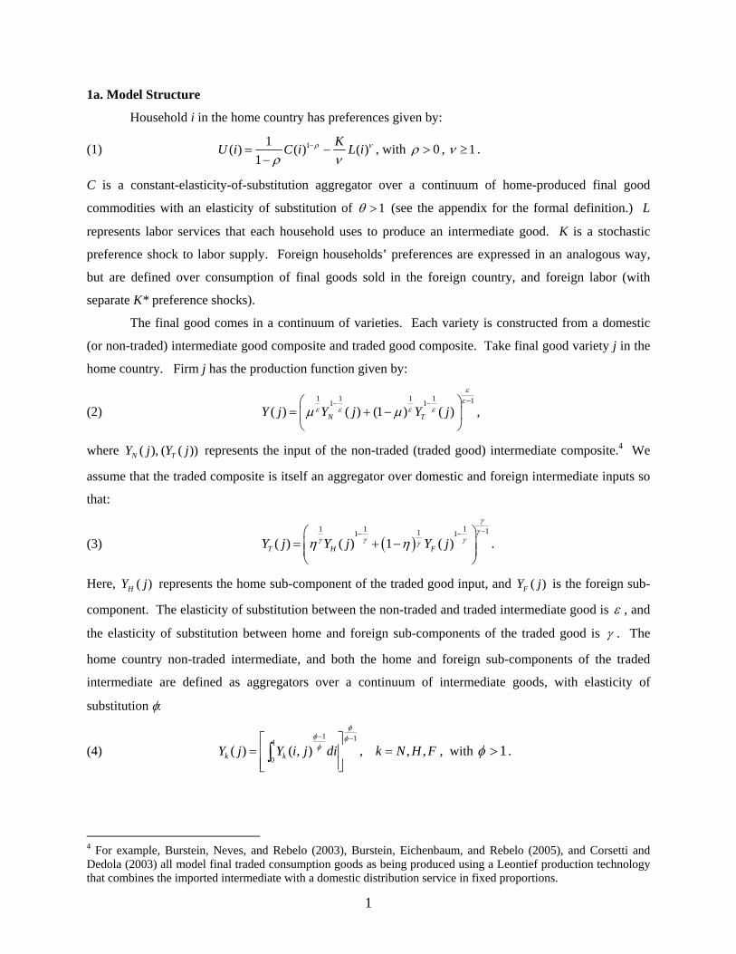
separate K* preference shocks). The final good comes in a continuum of varieties. Each variety is constructed from a domestic

(or non-traded) intermediate good composite and traded good composite. Take final good variety j in the

home country. Firm j has the production function given by:

(2) 1 1 1 1 11 1

( ) ( ) (1 ) ( )N TY j Y j Y j

εε

ε ε ε εµ µ−− −⎛ ⎞

= + −⎜ ⎟⎝ ⎠

,

where represents the input of the non-traded (traded good) intermediate composite.( ), ( ( ))N TY j Y j 4 We

assume that the traded composite is itself an aggregator over domestic and foreign intermediate inputs so

that:

(3) ( )1 1 1 111 1

( ) ( ) 1 ( )T H FY j Y j Y j

γγ

γ γ γγη η−− −⎛ ⎞

= + −⎜ ⎟⎜ ⎟⎝ ⎠

.

Here, represents the home sub-component of the traded good input, and is the foreign sub-

component. The elasticity of substitution between the non-traded and traded intermediate good is

( )HY j ( )FY j

ε , and

the elasticity of substitution between home and foreign sub-components of the traded good is γ . The

home country non-traded intermediate, and both the home and foreign sub-components of the traded

intermediate are defined as aggregators over a continuum of intermediate goods, with elasticity of

substitution φ:

(4) 1 11

0( ) ( , ) , , ,k kY j Y i j di k N H F

φφ φφ− −⎡ ⎤

= =⎢ ⎥⎢ ⎥⎣ ⎦∫ , with 1φ > .

4 For example, Burstein, Neves, and Rebelo (2003), Burstein, Eichenbaum, and Rebelo (2005), and Corsetti and Dedola (2003) all model final traded consumption goods as being produced using a Leontief production technology that combines the imported intermediate with a domestic distribution service in fixed proportions.

1

Home households consume all of each home final good variety . All home intermediate goods are

produced by home households using a technology linear in labor, so that

( )Y j

( , ) ( , ), ,kY i j L i j k N H= = , and

analogously for the foreign country’s intermediate goods.

The foreign country’s production function for traded goods is symmetric to the home country’s

but not identical. That is, using a * to denote foreign country quantities, we have:

( )1 1 1 111 1

* * *( ) ( ) 1 ( )T F HY j Y j Y j

γγ

γ γ γγη η−− −⎛ ⎞

= + −⎜ ⎟⎜ ⎟⎝ ⎠

.

There is home bias in the production of the traded aggregate if 1/ 2η > .

1.b A Flexible Price Model

We first outline a flexible-price version of the model. Since our primary interest is in how sticky

prices influence optimal exchange rate policy, we wish to eliminate any other sources of inefficiency that

are not directly related to price stickiness. One distortion arises due to monopoly pricing wedges in both

intermediate and final goods sectors. To avoid these, we assume that firms receive a per unit subsidy on

production so as to ensure that price would equal marginal cost at both the intermediate and final goods

level if all prices were fully flexible. The subsidy is financed by lump sum profit taxes on the firms.

A second issue is the nature of international capital markets. Again, to focus exclusively on the

constraints that are related to nominal rigidities, we assume that agents can engage in ex-ante cross

country trade in a full set of nominal state contingent assets. This ensures that if all prices were flexible,

full cross-country risk sharing would obtain.

Rather than explicitly introducing a role for money in the model, we simply define monetary

policy as a rule that targets the value of nominal consumption in each country. This is consistent with a

variety of alternative underlying models of money, such as money in the utility function, or a cash-in-

advance specification.5

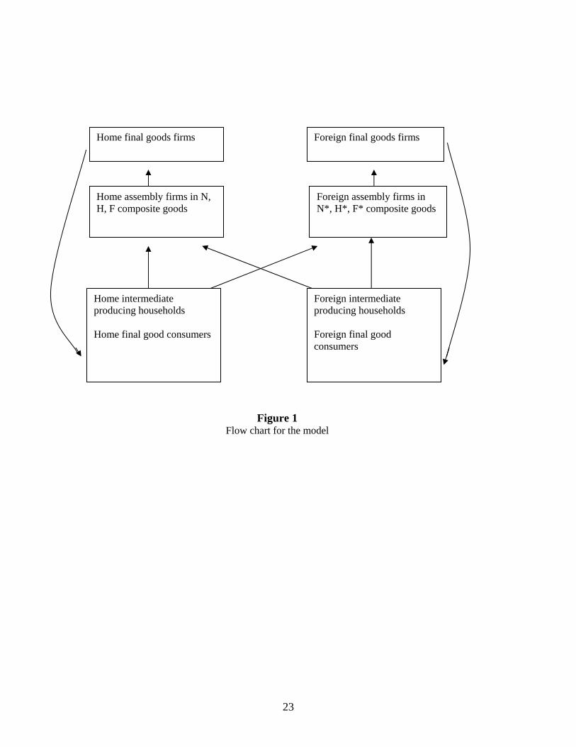
The structure of the model is illustrated in Figure 1. Basic intermediate goods are produced and

sold by monopolistically competitive producers (households) to assembly-type firms in the traded and the

non-traded sectors (for instance, the assembly firm in the traded good sector used production function (3)

written in an extensive form over each variety of home and foreign traded good using (4)). We assume

there is free entry into assembly and these firms simply sell at cost to final goods firms. Final goods are

differentiated, and each firm purchases the assembled intermediate traded and non-traded good

composites, produces using the production function (2), and sells its particular variety of final good to

domestic consumers, as a monopolistic competitor.

5 So long as money was fully neutral in the flexible price economy, our results would be unaltered by explicitly introducing the monetary side of the model.

2

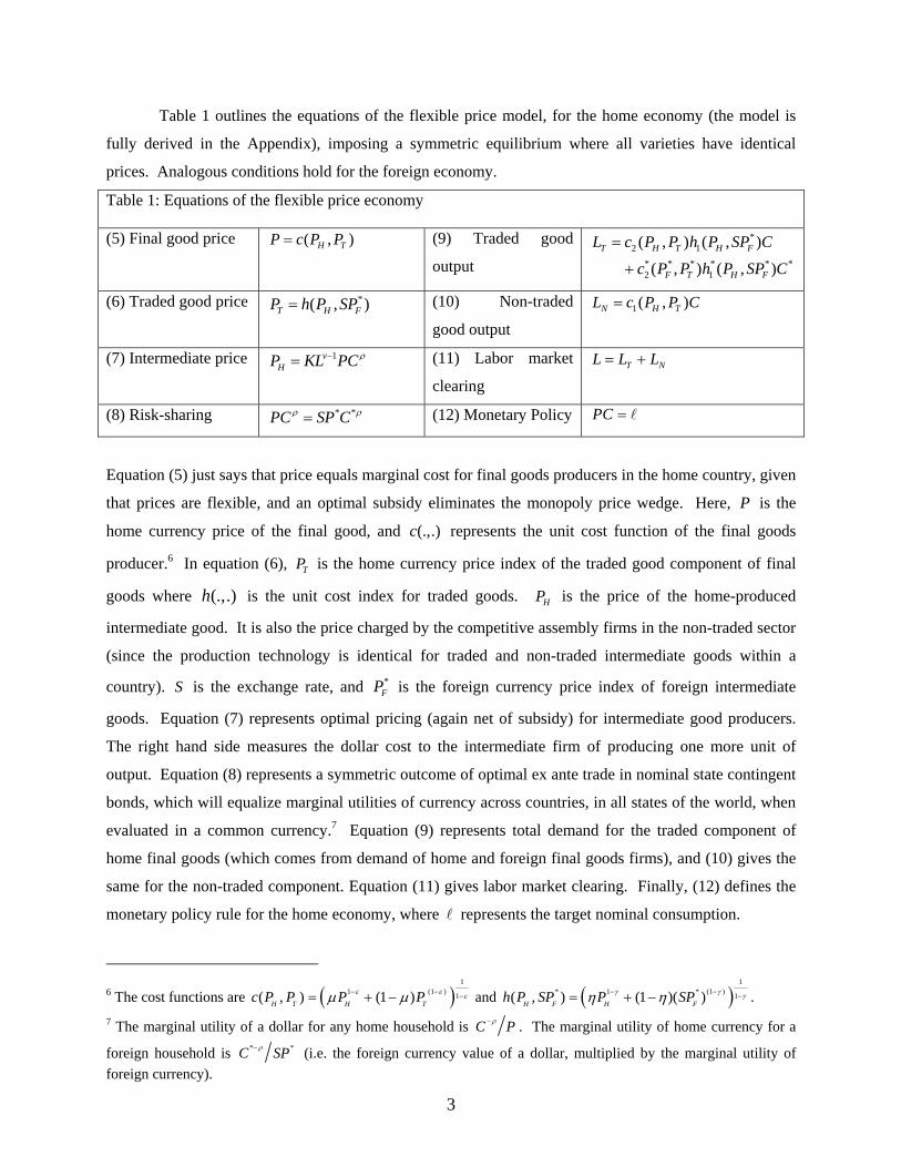
Table 1 outlines the equations of the flexible price model, for the home economy (the model is

fully derived in the Appendix), imposing a symmetric equilibrium where all varieties have identical

prices. Analogous conditions hold for the foreign economy. Table 1: Equations of the flexible price economy

(5) Final good price ( ,H TP c P P= ) (9) Traded good

output

*2 1

* * * * * *2 1

( , ) ( , )

( , ) ( , )T H T H F

F T H F

L c P P h P SP C

c P P h P SP C

=

+

(6) Traded good price *( , )T HP h P SP= F (10) Non-traded

good output 1( , )N H TL c P P C=

(7) Intermediate price 1vHP KL PCρ−= (11) Labor market

clearing T NL L L= +

(8) Risk-sharing * *PC SP Cρ ρ= (12) Monetary Policy PC =

Equation (5) just says that price equals marginal cost for final goods producers in the home country, given

that prices are flexible, and an optimal subsidy eliminates the monopoly price wedge. Here, is the

home currency price of the final good, and represents the unit cost function of the final goods

producer.

P

(.,.)c6 In equation (6), is the home currency price index of the traded good component of final

goods where is the unit cost index for traded goods. is the price of the home-produced

intermediate good. It is also the price charged by the competitive assembly firms in the non-traded sector

(since the production technology is identical for traded and non-traded intermediate goods within a

country). is the exchange rate, and

TP

(.,.)h HP

S *FP is the foreign currency price index of foreign intermediate

goods. Equation (7) represents optimal pricing (again net of subsidy) for intermediate good producers.

The right hand side measures the dollar cost to the intermediate firm of producing one more unit of

output. Equation (8) represents a symmetric outcome of optimal ex ante trade in nominal state contingent

bonds, which will equalize marginal utilities of currency across countries, in all states of the world, when

evaluated in a common currency.7 Equation (9) represents total demand for the traded component of

home final goods (which comes from demand of home and foreign final goods firms), and (10) gives the

same for the non-traded component. Equation (11) gives labor market clearing. Finally, (12) defines the

monetary policy rule for the home economy, where represents the target nominal consumption.

6 The cost functions are ( )

11 (1 1( , ) (1 )H T H Tc P P P Pε ε ) εµ µ− − −= + − and ( )

1* 1 * (1 ) 1( , ) (1 )( )H F H Fh P SP P SPγ γ γη η− − −= + − .

7 The marginal utility of a dollar for any home household is C Pρ− . The marginal utility of home currency for a

foreign household is *C SPρ− * (i.e. the foreign currency value of a dollar, multiplied by the marginal utility of foreign currency).

3

Equation (5), (6), (7) and (9)-(12) have counterparts for the foreign country, determining foreign

final goods prices, prices of foreign intermediate goods, foreign market clearing, and the foreign

monetary policy rule. The unit cost functions for the foreign final good may be written as * * *( , )F Tc P P and

*( , *)H Fh P S P . These equations for the home and foreign economy, together with equation (5), the risk

sharing rule, may be solved for the equilibrium values of ,

and

* * * * *, , , , , , , , , , , ,T N T N H F T TC C L L L L L L P P S P P P*

*P .

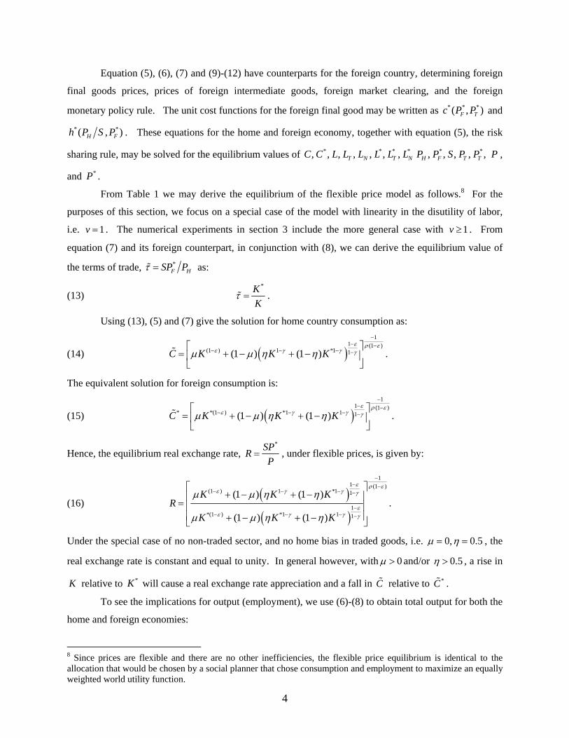
From Table 1 we may derive the equilibrium of the flexible price model as follows.8 For the

purposes of this section, we focus on a special case of the model with linearity in the disutility of labor,

i.e. . The numerical experiments in section 3 include the more general case with . From

equation (7) and its foreign counterpart, in conjunction with (8), we can derive the equilibrium value of

the terms of trade,

1v = 1v ≥

*F HSP Pτ = as:

(13) *K

Kτ = .

Using (13), (5) and (7) give the solution for home country consumption as:

(14) ( )1

1 (1 )(1 ) 1 *1 1(1 ) (1 )C K K K

ε ρ εε γ γ γµ µ η η

−− −

− − − −⎡ ⎤

= + − + −⎢ ⎥⎣ ⎦

.

The equivalent solution for foreign consumption is:

(15) ( )1

1 (1 )* *(1 ) *1 1 1(1 ) (1 )C K K K

ε ρ εε γ γ γµ µ η η

−− −

− − − −⎡ ⎤

= + − + −⎢ ⎥⎣ ⎦

.

Hence, the equilibrium real exchange rate, *SPR

P= , under flexible prices, is given by:

(16) ( )( )

11 (1 )

(1 ) 1 *1 1

1*(1 ) *1 1 1

(1 ) (1 )

(1 ) (1 )

K K KR

K K K

ε ρ εε γ γ γ

εε γ γ γ

µ µ η η

µ µ η η

−− −

− − − −

−− − − −

⎡ ⎤+ − + −⎢ ⎥= ⎢ ⎥

⎢ ⎥+ − + −⎣ ⎦

.

Under the special case of no non-traded sector, and no home bias in traded goods, i.e. 0, 0.5µ η= = , the

real exchange rate is constant and equal to unity. In general however, with 0µ > and/or 0.5η > , a rise in

relative to K *K will cause a real exchange rate appreciation and a fall in relative to . C *C

To see the implications for output (employment), we use (6)-(8) to obtain total output for both the

home and foreign economies:

8 Since prices are flexible and there are no other inefficiencies, the flexible price equilibrium is identical to the allocation that would be chosen by a social planner that chose consumption and employment to maximize an equally weighted world utility function.

4

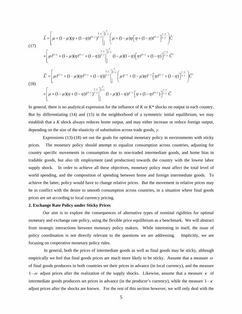
(17)

1 11 11 1

1 11 1 11 1

(1 )( (1 ) ) (1 ) (1 )

(1 )( (1 )) (1 )(1 ) (1 )

L C

C

εε γ εε

γ γγ γ

εε γ εε

ε γ γγ γ

µ µ η η τ µ µ η η η τ

µτ µ ητ η µ η ητ η

− −−− −− −

− −−− − −− −

⎡ ⎤ ⎛ ⎞⎡ ⎤= + − + − + − + −⎢ ⎥ ⎜ ⎟⎣ ⎦

⎢ ⎥ ⎝ ⎠⎣ ⎦

⎡ ⎤⎡ ⎤+ + − + − − − + −⎢ ⎥ ⎣ ⎦

⎢ ⎥⎣ ⎦

*

(18)

1 1* 1 1 11 1

1 11 11 1

(1 )( (1 )) (1 ) (1 )

(1 )( (1 ) ) (1 )(1 ) (1 )

L C

C

εε γ εε

ε γ ε γ γγ γ

εε γ εε

γ γ γγ γ

µτ µ ητ η µτ µ ητ ητ η

µ µ η η τ µ η τ η ητ

− −−− − − − −− −

− −−− − −− −

⎡ ⎤ ⎛ ⎞⎡ ⎤= + − + − + − + −⎢ ⎥ ⎜ ⎟⎣ ⎦

⎢ ⎥ ⎝ ⎠⎣ ⎦

⎡ ⎤⎡ ⎤+ + − + − − − + −⎢ ⎥ ⎣ ⎦

⎢ ⎥⎣ ⎦

*

In general, there is no analytical expression for the influence of K or K* shocks on output in each country.

But by differentiating (14) and (15) in the neighborhood of a symmetric initial equilibrium, we may

establish that a K shock always reduces home output, and may either increase or reduce foreign output,

depending on the size of the elasticity of substitution across trade goods, γ.

Expressions (13)-(18) set out the goals for optimal monetary policy in environments with sticky

prices. The monetary policy should attempt to equalize consumption across countries, adjusting for

country specific movements in consumption due to non-traded intermediate goods, and home bias in

tradable goods, but also tilt employment (and production) towards the country with the lowest labor

supply shock. In order to achieve all these objectives, monetary policy must affect the total level of

world spending, and the composition of spending between home and foreign intermediate goods. To

achieve the latter, policy would have to change relative prices. But the movement in relative prices may

be in conflict with the desire to smooth consumption across countries, in a situation where final goods

prices are set according to local currency pricing.

2. Exchange Rate Policy under Sticky Prices

Our aim is to explore the consequences of alternative types of nominal rigidities for optimal

monetary and exchange rate policy, using the flexible price equilibrium as a benchmark. We will abstract

from strategic interactions between monetary policy makers. While interesting in itself, the issue of

policy coordination is not directly relevant to the questions we are addressing. Implicitly, we are

focusing on cooperative monetary policy rules.

In general, both the prices of intermediate goods as well as final goods may be sticky, although

empirically we feel that final goods prices are much more likely to be sticky. Assume that a measure ω

of final goods producers in both countries set their prices in advance (in local currency), and the measure

1 ω− adjust prices after the realization of the supply shocks. Likewise, assume that a measure κ of

intermediate goods producers set prices in advance (in the producer’s currency), while the measure 1 κ−

adjust prices after the shocks are known. For the rest of this section however, we will only deal with the

5

extremes where a) all final goods prices are sticky and all intermediate prices flexible i.e. 1, 0ω κ= = , b)

all final goods prices are flexible and all intermediates prices are sticky 0, 1ω κ= = , or c) (in a special

case – see below) all prices of all goods are sticky 1, 1ω κ= = . In each of these cases, monetary policy

can exactly attain the flexible price equilibrium. In section 2 below, we analyze more general model

where the full flexible price allocation cannot be attained.

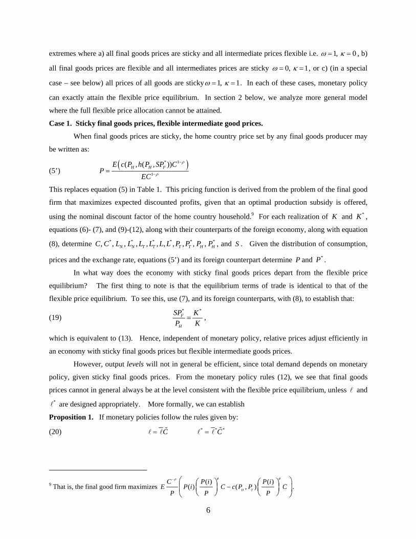
Case 1. Sticky final goods prices, flexible intermediate good prices.

When final goods prices are sticky, the home country price set by any final goods producer may

be written as:

(5’) ( )* 1

1

( , ( , ))H H FE c P h P SP CP

EC

ρ

ρ

−

−=

This replaces equation (5) in Table 1. This pricing function is derived from the problem of the final good

firm that maximizes expected discounted profits, given that an optimal production subsidy is offered,

using the nominal discount factor of the home country household.9 For each realization of and K *K ,

equations (6)- (7), and (9)-(12), along with their counterparts of the foreign economy, along with equation

(8), determine , and S . Given the distribution of consumption,

prices and the exchange rate, equations (5’) and its foreign counterpart determine and

* * * * *, , , , , , , , , , ,N N T T T T H HC C L L L L L L P P P P*

P *P .

In what way does the economy with sticky final goods prices depart from the flexible price

equilibrium? The first thing to note is that the equilibrium terms of trade is identical to that of the

flexible price equilibrium. To see this, use (7), and its foreign counterparts, with (8), to establish that:

(19) * *

F

H

SP KP K

= ,

which is equivalent to (13). Hence, independent of monetary policy, relative prices adjust efficiently in

an economy with sticky final goods prices but flexible intermediate goods prices. However, output levels will not in general be efficient, since total demand depends on monetary

policy, given sticky final goods prices. From the monetary policy rules (12), we see that final goods

prices cannot in general always be at the level consistent with the flexible price equilibrium, unless and

are designed appropriately. More formally, we can establish *

Proposition 1. If monetary policies follow the rules given by:

(20) C= * *C= *

9 That is, the final good firm maximizes ( ) ( )

( ) ( , )H T

C P i P iE P i C c P P C

P P P

φ φρ−

−⎛ ⎞⎛ ⎞ ⎛ ⎞

⎜ ⎟ ⎜ ⎟⎜ ⎟⎝ ⎠ ⎝ ⎠⎝ ⎠.

6

where and * are arbitrary constant parameters, then the equilibrium with sticky final goods prices

coincides with the flexible price equilibrium, with P = and * *P = .

Proof: See Appendix.

The proposition ensures that flexible price equilibrium real exchange rate is attained, since the

monetary rules combined with (8) imply that * *

* *

SP P CP P C

ρρ⎛ ⎞⎛ ⎞

= = ⎜ ⎟⎜ ⎟⎝ ⎠ ⎝ ⎠

and each country’s consumption

is equal to its flexible price equilibrium level. The optimal monetary policies eliminate the distortion due

to sticky final goods prices. An alternative way to see it is that the monetary rules stabilize marginal cost

for final goods producers, so that equation (5) always holds, even with sticky final goods prices. Final

goods firms would not wish to adjust their prices even if they could.

What do these monetary policy rules imply with respect to exchange rate movements? Since

final goods prices are state independent, then the exchange rate moves in proportion to relative

consumption movements. Using (14) and (15), and taking a first order approximation around an initial

symmetric equilibrium, where we define ˆ ln( ) ln( )X X E X≡ − , we establish that under the optimal

monetary policy the real exchange rate behaves as:

(21) ( ) *ˆ ˆ(2 1)(1 ) ( )ˆR K Kµ η µ= − + − − −

From (21) we note that if all intermediate goods are traded ( 0µ = ), and there is no home bias in the

traded intermediate good ( 0.5η = ), then the real exchange rate response to shocks is zero. In that case,

the optimal policy fixes the nominal exchange rate. Although all intermediates are traded and there is no

home bias, we might still expect that exchange rate movement would be necessary to achieve efficient

relative price (terms of trade) adjustment. But when intermediate good prices are fully flexible the

desired terms of trade adjustment is fully achieved by movements in *H FP P , without any movements in

the exchange rate. In fact, a fixed exchange rate is in this case a necessary part of an optimal policy, since

any exchange rate movement would generate undesirable real exchange rate volatility, and a departure

from optimal risk sharing. More generally, when 0µ > or 0.5η > , the optimal policy requires some real exchange rate

policy. In this case, the nominal exchange rate must move, since in order to facilitate different

movements in home consumption, relative to foreign consumption, the real exchange rate must move.

Note however that the volatility of the optimal real exchange rate will always be less than that of the

flexible price equilibrium terms of trade. Irrespective of home bias or non-traded intermediate inputs, an

optimal monetary policy would never produce as much nominal exchange rate variability as necessary to

reproduce the volatility of the flexible price terms of trade.

7

Proposition 1 implies that when all intermediate goods prices are flexible, optimal policy faces no

trade-off. The optimal real exchange rate can be achieved, while simultaneously achieving efficient

relative price adjustment. In fact, if any fraction of final goods prices is set in advance in consumers’

currencies, Proposition 1 holds without change. The logic is simple: if monetary policy continues to

stabilize marginal cost for final goods, final goods firms that are free to adjust will choose to leave their

prices unchanged. That is, with these monetary policies, flexible price firms lose nothing by acting just

like sticky-price firms and not adjusting prices in response to shocks. The same equilibrium obtains as in

the fully sticky-price case. Hence, when 0µ = and 0.5η = , as long as intermediate goods prices are

fully flexible, then any amount of price rigidity at the final goods level implies that fixing the exchange

rate is optimal.10

Case 2. Sticky intermediate goods prices, flexible final good prices.

Now we look at the polar opposite case. Say that final goods prices are fully flexible, but

intermediate goods prices are sticky. While this case may be empirically less plausible than the previous

case, it illustrates again the dual objectives of exchange-rate policy: achieving desired terms of trade

changes, but avoiding undesirable real exchange rate changes. With sticky intermediate goods prices, condition (7) becomes:

(7’) ( )H

E KLPLE

PC ρ

=⎛ ⎞⎜ ⎟⎝ ⎠

.

This condition says that when the intermediate producer must set their prices in advance, they

trade off the expected marginal utility benefit of a price reduction in terms of greater sales, with the

expected marginal utility cost in terms of greater work effort.11 An equilibrium of the model with sticky

intermediate goods prices is defined by the values for and S that

solve (5), (6), (9)-(12) and their foreign counterparts, and (8), for each realization of

* * * * *, , , , , , , , , , ,N N T T T TC C L L L L L L P P P P*

*,K K . Then

and

HP

*FP may be solved from (7’) and its foreign counterpart.

10 There is a distinction between an outcome in which monetary policy delivers a fixed exchange rate as part of an optimal rule, as we find here, and an exchange rate policy which imposes a mandatory peg, irrespective of the nature of shocks. For instance, in the case 0µ = , 0.5η = , pegging the exchange rate without following the policies implied by proposition 1 would not achieve a welfare optimum.

11 Home country intermediate good producer j maximizes 1 ( )( )

( )(1 )1

HH H

H

P jC jE KP j s

P

φρ

ρ

−−

− +−

⎛ ⎞⎛ ⎞⎜ ⎟⎜ ⎟⎜ ⎟⎝ ⎠⎝ ⎠

HX , where

is a linear function of intermediate demand, given by ( )C j( )H

H

H

P jX

P

φ−

⎛ ⎞⎜ ⎟⎝ ⎠

, and Hs is the subsidy on intermediate

goods.

8

In the previous case, we found that even with sticky final goods prices, price flexibility at the

intermediate goods level achieved an efficient response of the terms of trade. But with sticky

intermediate goods prices, getting the terms of trade to move requires an equal exchange rate response.

Moreover, because the terms of trade affects the real exchange rate, a failure to sustain the optimal the

terms of trade response will carry over into an inefficient real exchange rate, and deviations from optimal

risk sharing, even though final goods prices are fully flexible. Only when 0µ = and 0.5η = do we find

an efficient real exchange rate, because then, with final goods prices flexible, PPP always holds, and

consumption is equalized across countries.

In the presence of sticky intermediate goods prices, but flexible final goods prices, an optimal

monetary policy must ensure that the nominal exchange rate adjusts so as to achieve the efficient response

of the terms of trade. From (8) and (12), the nominal exchange rate may be written implicitly as 1

* *

PSP

ρ ρ−⎛ ⎞ ⎛ ⎞= ⎜ ⎟ ⎜ ⎟⎝ ⎠ ⎝ ⎠

We may then establish

Proposition 2. If the monetary policies are:

(22) 1 1

K Pρ

ρ ρ−

− −=

1 1* * *K P

ρρ ρ

−− −

= ,

where and * are arbitrary constant parameters, then the equilibrium with sticky intermediate good

prices achieves the same allocation as the flexible price equilibrium, with HP ρ= and * *FP ρ= .

Proof: See Appendix.

In this case, the exchange rate is equal to *( ) ( )H FS Pρ *Pτ τ= = . The exchange rate must

adjust so as to ensure that the terms of trade is equal to its flexible price equilibrium level in each state of

the world. The optimal monetary policy replicates the flexible price equilibrium, because it keeps the

marginal cost of intermediate goods firms constant, so that (7) and its foreign counterpart hold, even with

sticky intermediate goods prices. Again, this is a case where there is no trade-off between the exchange

rate that is desirable for consumption allocations and that needed for terms of trade adjustment. Because

final goods prices are flexible, the efficient real exchange rate is attained so long as the efficient terms of

trade is attained, ensuring efficient consumption allocations in each state. But because nominal prices of

intermediate goods cannot change, exchange rate adjustment is necessary to attain the efficient terms of

trade. Note that unlike the previous case, where the optimal nominal exchange rate volatility is always

less than the flexible price equilibrium terms of trade volatility, in this case they are equal. Volatility in

the real exchange rate is below the volatility in the terms of trade, since the optimal real exchange rate

response is attained by having domestic prices move in an offsetting direction.

9

As before, we can extrapolate to the case where some but not all intermediate goods prices are

sticky. So long as a fraction of prices cannot adjust, Proposition 2 still holds. If monetary policy

stabilizes marginal cost for intermediate good producers, those producers that can adjust prices will not

wish to, and relative price adjustment is fully achieved by nominal exchange rate adjustment.

Case 3. A special case of fixed proportions technologies

What happens if both final goods prices and intermediate goods prices are sticky? In general, this

leaves monetary policy incapable of fully achieving the socially optimal allocation. Following the

monetary rule of proposition 1 would ensure efficient consumption risk sharing, but would not achieve

the desired terms of trade adjustment, so that the allocation of production across countries would not be

efficient.

But there is a particular case where both objectives may be met, even when all prices are sticky.

Assume that there is no home bias, and all intermediate goods are traded. That is, 0µ = and 0.5η = .

Then let domestic and foreign intermediates be perfect complements in production; that is, 0γ = . In this

case, the production function takes on a fixed proportions form. From (14) and (15), the flexible price

equilibrium is:

(23) ( )1

* * * 10.5 0.5FP FP FP FP vC C L L K K ρ−+ −= = = = + ,

where FP stands for `fixed proportions’. In this case, the flexible price equilibrium would equalize not only consumption across countries,

but also output levels. Since relative output is independent of K shocks, we might guess that relative

price adjustment is not a priority. Engel (2002) notes that the expenditure-switching role of exchange rate

adjustment depends critically on the substitutability of inputs in production. When substitutability is low,

then expenditure switching is not important. We have:

Proposition 3: When 0µ = , 0.5η = , and 0γ = , and the monetary policy rules are given by:

(24) FPC= * * FPC= ,

where and * are arbitrary constant parameters, then the equilibrium where both final goods prices and

intermediate goods prices are sticky coincides with the flexible price equilibrium, with P = and * *P = .

Proof: See Appendix.

Since PPP holds in this case, the exchange rate is *S P P= = * , and state independent.

Again, a fixed exchange rate is necessary for efficient consumption allocations. Now this holds even with

sticky intermediate goods prices, because with fixed proportions technology no relative price adjustment

10

is necessary to facilitate expenditure switching, so there is no trade-off between consumption efficiency

and terms of trade adjustment.12

In considering empirically the size of this elasticity of substitution, we should focus on the short

run. We are considering in this context the role of exchange rate movements as a method of ameliorating

the distortions introduced by sticky prices. The horizon for such considerations is determined by the

speed of adjustment of nominal prices. But the short-run elasticity of substitution of imported

intermediate inputs is likely to be quite low.

Combination Policies

Returning now to the more general case with positive elasticity of substitution across intermediate

goods, we can see that the essence of the problem is that when policymakers must deal with two types of

price stickiness, monetary policy on its own is not sufficient to achieve a first best outcome. The

exchange rate response that achieves efficient risk sharing is smaller than that which ensures the optimal

terms of trade adjustment. But if the policy-makers had access to both monetary and fiscal policy tools, it

would be relatively easy to sustain a first best allocation, using a combination of monetary policy

adjustment and state varying commodity taxes or subsidies. For instance, take the case where both

intermediate good prices and final goods prices are all pre-set. Even with an optimal monetary policy, the

policy-maker cannot ensure that the terms of trade adjusts as in (13), and the real exchange rate adjusts as

in (16). But if monetary policy were designed as in (20), so as to target the efficient real exchange rate,

then it is easy to design a policy of state varying taxes and subsidies applied on the purchases of

intermediate composites from the assembly firms which would ensure the desired degree of expenditure

switching across home and foreign intermediate goods, even with sticky intermediate goods prices. For

instance, if the pre-set price of the intermediate goods are and HP FP , then the after tax price paid by

final goods firms is and (1 )H HP t+ (1 )F FP t+ . A tax policy which sets the after tax prices such that

(1 )

*(1 )H HKP tK

µ η µ+ −⎛ ⎞+ = ⎜ ⎟⎝ ⎠

and (1 )(1 )*

(1 )F FKP tK

η µ− −⎛ ⎞

+ = ⎜ ⎟⎝ ⎠

(and analogous tax rates for the foreign country)

will ensure that a) final goods firms face the efficient relative prices for intermediate good composites,

and b) the unit cost of final goods firms is constant, so that the firms have no incentive to alter the final

goods price, even if prices were flexible. This policy acts so as to tax the use of the intermediate that

suffers the relatively negative labor supply shock and subsidize the intermediate which receives the

relatively positive shock.

12 Note that equation (13) indicates that the terms of trade will still respond to shocks when 0γ = . But this is not

allocative, since from (23), in this case, and therefore any monetary rule that targets overall world output can achieve the efficient outcome without any relative price change.

*L L=

11

In general though, we may not be able to rely on a set of state varying taxes and subsidies to

achieve efficient relative price adjustment. In this case, monetary policy alone must face the trade-off

across objectives. We focus on this trade-off in the next section.

3. The General Trade-off between Terms of Trade adjustment and Deviations from PPP

In the previous section, we showed that if final goods prices are partially or fully pre-set but all

intermediate goods prices are free to adjust, then an optimal monetary rule stabilizes the exchange rate

relative to the terms of trade, and in some cases actually delivers a fixed exchange rate. On the other

hand, if intermediate goods prices are partially or fully sticky but all final goods prices are flexible, then

an optimal monetary rule uses the exchange rate to replicate the terms of trade adjustment that would take

place in a flexible price economy. More realistically however, both final goods prices and intermediate

goods prices are likely to be partially sticky. We now extend the model to allow for this. Now we find

that there is a real trade-off. Except when foreign and domestic inputs are perfect complements (and all

intermediate goods are traded), monetary policy cannot remove all distortions. Hence, our interest in this

section is quantitative. For different degrees of price stickiness at the intermediate and final goods level,

how much exchange rate volatility should be allowed so as to facilitate relative price adjustment (or

expenditure switching), at the cost of weakening the efficiency of cross-country consumption allocations?

Following this direction, we now let ω (the measure of final goods producers who set their

prices in advance, in the consumer’s currency), and κ (the measure of intermediate goods producers who

set prices in advance in the producer’s currency) fall between zero and one. Empirically, our prior would

be that ω κ> , but we do not impose this in the simulations.

In a symmetric equilibrium, the price index for final goods is written as

1

1 1 1ˆ (1 )P P Pθ θ θω ω− − −⎡ ⎤= + −⎣ ⎦ ,

where a indicates the price of a good that is set in advance, and P P indicates the ex-post flexible price.

The flexible price P is just equal to marginal cost, as before, whereas is defined by the condition: P

(25) ( )1

1

111 1 *1 1

1 1

(1 )( (1 ) )ˆ

H H FE P P P C P

PE C P

εγ εε γ γ ρ

ρ θ

µ µ η η−− −− − − −

− −

⎡ ⎤+ − + −⎢ ⎥

⎢ ⎥⎣ ⎦=⎡ ⎤⎣ ⎦

1θ −

,

which differs from (5’) due to the fact that the aggregate price index is now stochastic. P

The intermediate good price index is:

( )1

1 1 1ˆ (1 )H H HP P Pφ φ φκ κ− − −= + − ,

where again, is the sticky price of the intermediate good, and HP HP is the flexible price. The flexible

price intermediate is set as:

12

(26)

1v

HH

H

PP K L PCP

φρ

−−⎛ ⎞⎛ ⎞⎜ ⎟= ⎜ ⎟⎜ ⎟⎝ ⎠⎝ ⎠

where the term inside the parentheses on the right hand side indicates that the relative price of fixed to

flexible-price intermediate goods affects the composition of demand facing price setters. The sticky price

of the intermediate good is written as:

(27) 1

ˆ

ˆˆ

v

H

H

H

H

H

PE K LP

PPE L P CP

φ

φ

ρ

−

−

− −

⎡ ⎤⎛ ⎞⎛ ⎞⎢ ⎥⎜ ⎟⎜ ⎟⎢ ⎥⎜ ⎟⎝ ⎠⎝ ⎠⎢ ⎥⎣ ⎦=⎡ ⎤⎛ ⎞⎢ ⎥⎜ ⎟⎢ ⎥⎝ ⎠⎣ ⎦

The risk sharing condition (5) is written as before, while the market clearing condition for output of the

intermediate good is written as:

(28) * *

** * *

ˆ(1 ) (1 )

ˆ(1 )(1 ) (1 )

H H

G I

H

I

P P P PL CP P P P

P P P CP P P

θε γ θ

θγ θ

µ µ η ω ω

µ η ω ω

−− − −

−− −

⎛ ⎞⎛ ⎞ ⎛ ⎞⎛ ⎞ ⎛ ⎞ ⎛ ⎞⎜ ⎟⎜ ⎟= + − + −⎜ ⎟⎜ ⎟ ⎜ ⎟ ⎜ ⎟⎜ ⎟⎜ ⎟⎜ ⎟⎝ ⎠⎝ ⎠⎝ ⎠ ⎝ ⎠⎝ ⎠⎝ ⎠⎛ ⎞⎛ ⎞⎛ ⎞ ⎛ ⎞⎜ ⎟+ − − + −⎜ ⎟⎜ ⎟ ⎜ ⎟⎜ ⎟⎜ ⎟⎝ ⎠⎝ ⎠ ⎝ ⎠⎝ ⎠

,

where we define1

1 1 1(1 )G H IP P Pε ε εµ µ− − −⎡ ⎤= + −⎣ ⎦ and 1

1 * 1 1(1 )( )I H FP P SPγ γ γη η− −−⎡ ⎤= + −⎣ ⎦ as the aggregate price

index for all intermediate goods and traded intermediate goods, respectively. An equivalent set of

conditions may be written for the foreign economy. An optimal monetary policy in this model is aimed at eliminating three types of distortions. First,

as before, there is an inefficiency due to the failure of efficient risk sharing, which leads to distorted

consumption allocations, or an inefficient distribution of consumption across countries. Second, there is

an inefficiency due to the lack of adjustment of the terms of trade (the relative price of the home and

foreign intermediate) to the labor supply shocks, which implies an inefficient allocation of production

across countries. Finally, there is a new inefficiency coming from the fact that with some intermediate

good prices set in advance, production levels will differ across sticky price and flexible price intermediate

goods firms, implying an inefficient allocation of production across firms within a country.

An optimal monetary rule cannot eliminate all these inefficiencies simultaneously, except in the

special cases of the previous section. Moreover, it is not possible to characterize the optimal monetary

policies analytically in this more general case. Rather, we solve the model numerically, choosing the

monetary policy that maximizes expected utility for a given calibration of parameter values and

distribution of labor supply shocks.

13

The model is entirely symmetric, so that home and foreign expected utility are identical when

monetary policies are identically chosen across countries. As in the previous section, we abstract from

issues of strategic interaction across policy makers and derive an optimal policy rule that maximizes an

equal-weighted sum of home and foreign expected utilities.

As emphasized by Obstfeld and Rogoff (2002), when shocks are global there is no need for terms

of trade change or exchange rate adjustment. Hence, we focus only on country specific labor supply

shocks, so that K+K* is constant. Moreover, we assume a two-state distribution of across the two

countries, where K is either high or low, and normalized so that the standard deviation of the terms of

trade in the flexible price economy is unity. In the benchmark version of the model, we assume that the

elasticity of substitution in consumption among all varieties of final goods and the elasticity of

substitution in production among all varieties in each of the non-traded, and home and foreign traded

intermediate aggregates are the same, 3

K

θ φ= = . We set the preference parameters 1 vρ = = (see Table

2 for the full list of parameters.) We impose unit elasticity of substitution both between home and foreign

intermediate goods and between traded and non-traded intermediate good, so that 1γ = and 1ε = . We

assume that the traded good composite has equal weights, so that 0.5η = , and we allow a range of values

for the non-traded intermediate weight µ . We also report results from alternative parameter settings

below. Assuming again that the monetary instrument is the nominal value of consumption in each

country, we simulate the model, searching across state contingent values of and that maximize

utility. Given these values, we can derive the variance of the exchange rate and the cross-country

correlation of consumption.

*

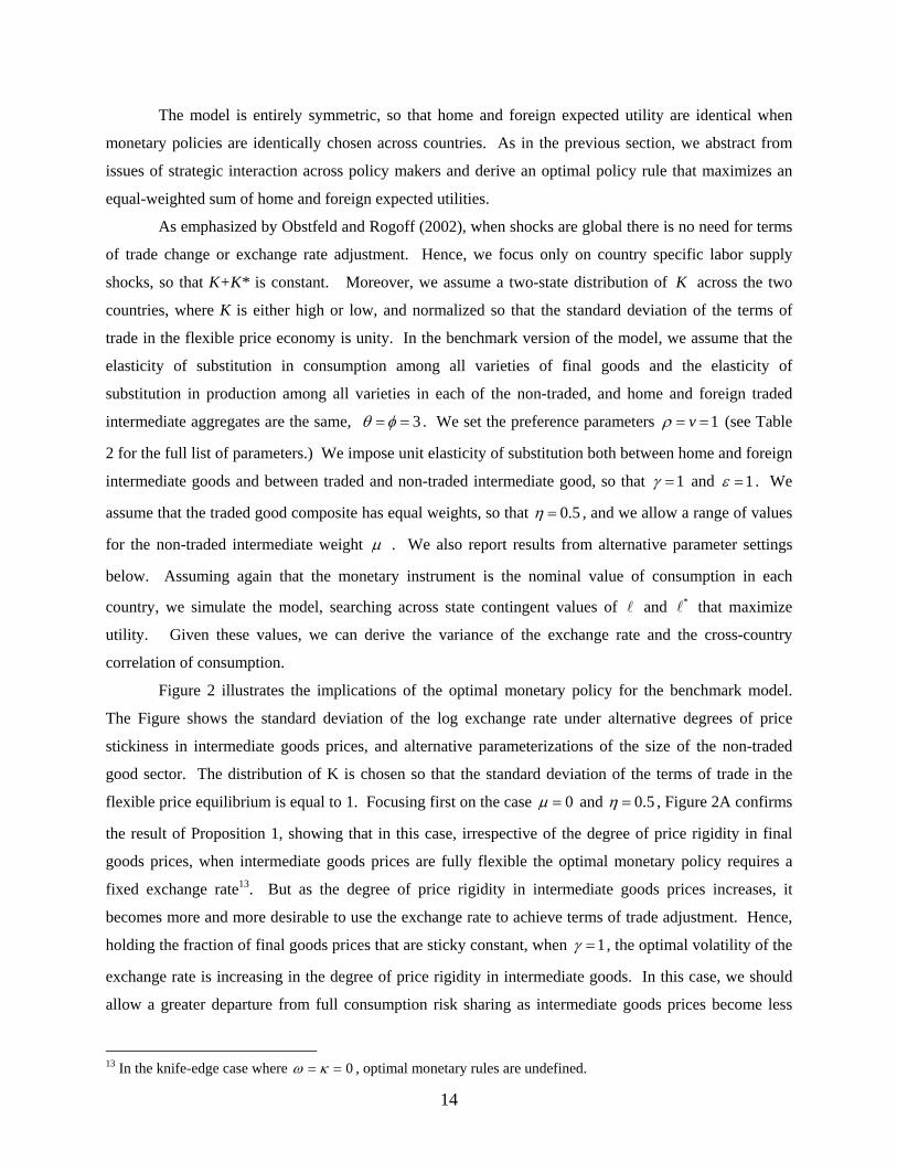
Figure 2 illustrates the implications of the optimal monetary policy for the benchmark model.

The Figure shows the standard deviation of the log exchange rate under alternative degrees of price

stickiness in intermediate goods prices, and alternative parameterizations of the size of the non-traded

good sector. The distribution of K is chosen so that the standard deviation of the terms of trade in the

flexible price equilibrium is equal to 1. Focusing first on the case 0µ = and 0.5η = , Figure 2A confirms

the result of Proposition 1, showing that in this case, irrespective of the degree of price rigidity in final

goods prices, when intermediate goods prices are fully flexible the optimal monetary policy requires a

fixed exchange rate13. But as the degree of price rigidity in intermediate goods prices increases, it

becomes more and more desirable to use the exchange rate to achieve terms of trade adjustment. Hence,

holding the fraction of final goods prices that are sticky constant, when 1γ = , the optimal volatility of the

exchange rate is increasing in the degree of price rigidity in intermediate goods. In this case, we should

allow a greater departure from full consumption risk sharing as intermediate goods prices become less

13 In the knife-edge case where 0ω κ= = , optimal monetary rules are undefined.

14

capable of adjusting to labor supply shocks. Since with 0µ = , consumption risk sharing should equalize

consumption across countries, the extent of the deviation from optimal risk sharing is measured by the

volatility in the nominal (and real) exchange rate. Note that although the optimal monetary policy allows

for exchange rate movement, exchange rate adjustment is far less than the terms of trade adjustment that

would occur in a frictionless economy. When a quarter of all intermediate goods have prices set in

advance, then the exchange rate volatility is only about a quarter of that in the flexible price model. Even

when , so that all intermediate goods prices are sticky, the standard deviation of the exchange rate

under an optimal monetary policy is only 0.5.

1κ =

Figure 2A also illustrates the actual volatility in the terms of trade, which is measured by the log

standard deviation of *

F

H

SPP

. When 0κ = , Proposition 1 applies, and this is equal to unity (the flexible

price terms of trade volatility). As rises, the volatility falls below 1. The key feature of the trade-off

between terms of trade movement and consumption-risk sharing can be seen by the process of falling

volatility in the terms of trade, and a rising volatility of the nominal exchange rate, as rises. As

κ

κ 1κ → ,

the two coincide. Note however that optimal real exchange rate volatility is always below the optimal

terms of trade volatility.

As µ , the weight on non-traded intermediate goods in the production of final output, rises, the

optimal exchange rate volatility rises, as implied by Proposition 1. Setting 0.5µ = , Figure 2B indicates

that exchange rate volatility should be approximately 0.5 with fully flexible intermediate goods prices,

and rises to just over 0.7 as intermediate good prices become fully predetermined. In this case,

domestically oriented monetary policy is required to generate country specific consumption responses,

which requires exchange rate movements. But again, there is still a trade-off between the need to

generate efficient terms of trade movements and the goals of an efficient aggregate consumption

response. In particular, optimal exchange rate volatility is still less than both the flexible price and the

actual terms of trade volatility.

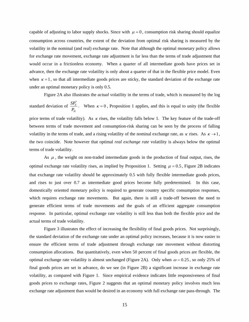
Figure 3 illustrates the effect of increasing the flexibility of final goods prices. Not surprisingly,

the standard deviation of the exchange rate under an optimal policy increases, because it is now easier to

ensure the efficient terms of trade adjustment through exchange rate movement without distorting

consumption allocations. But quantitatively, even when 50 percent of final goods prices are flexible, the

optimal exchange rate volatility is almost unchanged (Figure 2A). Only when 0.25ω = , so only 25% of

final goods prices are set in advance, do we see (in Figure 2B) a significant increase in exchange rate

volatility, as compared with Figure 1. Since empirical evidence indicates little responsiveness of final

goods prices to exchange rates, Figure 2 suggests that an optimal monetary policy involves much less

exchange rate adjustment than would be desired in an economy with full exchange rate pass-through. The

15

third locus in Figures 3 illustrates the volatility of the real exchange rate, which differs from nominal

exchange rate volatility when some final goods prices are flexible. Real exchange rate volatility is lower,

and the distance between actual and optimal real exchange rate volatility (zero) is less than that between

the actual and optimal terms of trade volatility.

Hence, the main message of the previous section continues to apply in the extended model: when

prices are sticky in local currency, an optimal monetary policy implies less exchange rate flexibility than

would be inferred from the traditional pricing model with full pass-through to consumer prices.

Moreover, despite local currency price stickiness in final goods, this is a model where there is a

substantial expenditure-switching role for the exchange rate in production, since there is full exchange

rate pass-through at the intermediate good level.

In Figures 2-3, the relationship between κ and exchange rate volatility is concave. As

intermediate goods prices become more and more sticky (for a given degree of price rigidity in final

goods), exchange rate volatility increases, but at a diminishing rate. As κ goes to unity, the gain from

terms of trade adjustment in response to exchange rate changes is offset by the costs in terms of reduced

consumption risk sharing. In fact, the numerical solution shows that the optimal monetary rules are

effectively independent of movements in κ , for values of κ greater than 0.5. This is true for all values

of ω . Hence, in the benchmark model, the benefit of further exchange rate adjustment in facilitating

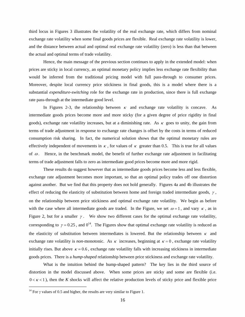
terms of trade adjustment falls to zero as intermediate good prices become more and more rigid. These results do suggest however that as intermediate goods prices become less and less flexible,

exchange rate adjustment becomes more important, so that an optimal policy trades off one distortion

against another. But we find that this property does not hold generally. Figures 4a and 4b illustrates the

effect of reducing the elasticity of substitution between home and foreign traded intermediate goods, γ ,

on the relationship between price stickiness and optimal exchange rate volatility. We begin as before

with the case where all intermediate goods are traded. In the Figure, we set 1ω = , and vary κ , as in

Figure 2, but for a smaller γ . We show two different cases for the optimal exchange rate volatility,

corresponding to 0.25γ = , and 014. The Figures show that optimal exchange rate volatility is reduced as

the elasticity of substitution between intermediates is lowered. But the relationship between κ and

exchange rate volatility is non-monotonic. As κ increases, beginning at 0κ = , exchange rate volatility

initially rises. But above , exchange rate volatility falls with increasing stickiness in intermediate

goods prices. There is a hump-shaped relationship between price stickiness and exchange rate volatility.

0.6κ =

What is the intuition behind the hump-shaped pattern? The key lies in the third source of

distortion in the model discussed above. When some prices are sticky and some are flexible (i.e.

), then the K shocks will affect the relative production levels of sticky price and flexible price 0 κ< < 1 14 For γ values of 0.5 and higher, the results are very similar to Figure 1.

16

firms. For instance, a positive home K shock will reduce the output of flexible price intermediate goods

firms relative to sticky price firms, in the home country. This creates a welfare loss15. It then becomes

desirable to reduce aggregate demand for the home intermediate good, through a tight monetary policy –

reducing the output of the sticky price firms and moving towards a more uniform pattern of production

across home intermediate firms. But this requires a home country currency appreciation. If by contrast,

, a shock will affect all home intermediate firms in the same way. The policymaker then has to

worry only about consumption allocations and terms of trade adjustment. For a very low elasticity of

substitution, the latter consideration is much less important (from Proposition 3). Hence, overall, moving

from an economy where half of all intermediate goods prices are fixed to one where all prices are fixed

can reduce the optimal exchange rate volatility.

1κ =

This result also reveals an interesting feature of our basic welfare trade-off. The expectation

might be that an optimal monetary policy would always want to reduce the volatility of the terms of trade

below its efficient level, while at the same time increasing the volatility of relative consumption growth

above the efficient level, as intermediate goods prices become less and less flexible. But when γ is

below unity, this is not necessarily the case. As κ rises above a certain level, it may be optimal to reduce

both terms of trade volatility as well as relative consumption volatility.

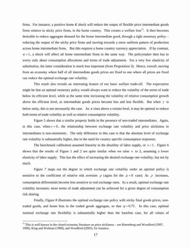
Figure 5 shows that a similar property holds in the presence of non-traded intermediates. Again,

in this case, when 0γ = , the relationship between exchange rate volatility and price stickiness in

intermediates is non-monotonic. The only difference in this case is that the absolute level of exchange

rate volatility is substantially higher, due to the need for country specific consumption responses.

The benchmark calibration assumed linearity in the disutility of labor supply, or . Figure 6

shows that the results of Figure 1 and 2 are quite similar when we raise to 2, assuming a lower

elasticity of labor supply. This has the effect of increasing the desired exchange rate volatility, but not by

much.

1v =

v

Figure 7 maps out the degree to which exchange rate volatility under an optimal policy is

sensitive to the coefficient of relative risk aversion ρ (again for the 0µ = case). As ρ increases,

consumption differentials become less sensitive to real exchange rates. As a result, optimal exchange rate

volatility increases: more terms of trade adjustment can be achieved for a given degree of consumption

risk sharing.

Finally, Figure 8 illustrates the optimal exchange rate policy with sticky final goods prices, non-

traded goods, and home bias in the traded goods aggregate, so that 0.75η = . In this case, optimal

nominal exchange rate flexibility is substantially higher than the baseline case, for all values of

15 This is well known in the closed economy literature on price stickiness – see Rotemberg and Woodford (1997, 1999), King and Wolman (1999), and Woodford (2003), for instance.

17

intermediate good price stickiness. But the qualitative relationship between real exchange rate flexibility

and terms of trade flexibility remains as before.

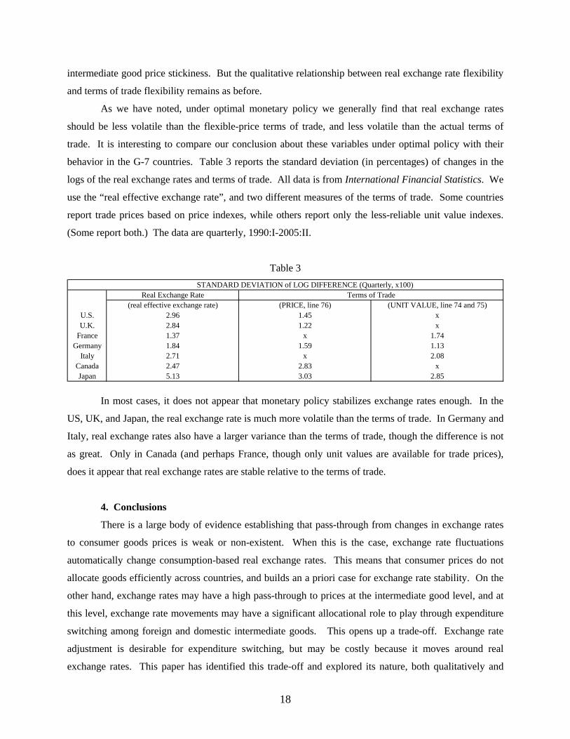
As we have noted, under optimal monetary policy we generally find that real exchange rates

should be less volatile than the flexible-price terms of trade, and less volatile than the actual terms of

trade. It is interesting to compare our conclusion about these variables under optimal policy with their

behavior in the G-7 countries. Table 3 reports the standard deviation (in percentages) of changes in the

logs of the real exchange rates and terms of trade. All data is from International Financial Statistics. We

use the “real effective exchange rate”, and two different measures of the terms of trade. Some countries

report trade prices based on price indexes, while others report only the less-reliable unit value indexes.

(Some report both.) The data are quarterly, 1990:I-2005:II.

Table 3

Real Exchange Rate(real effective exchange rate) (PRICE, line 76) (UNIT VALUE, line 74 and 75)

U.S. 2.96 1.45 xU.K. 2.84 1.22 x

France 1.37 x 1.74Germany 1.84 1.59 1.13

Italy 2.71 x 2.08Canada 2.47 2.83 xJapan 5.13 3.03 2.85

STANDARD DEVIATION of LOG DIFFERENCE (Quarterly, x100)Terms of Trade

In most cases, it does not appear that monetary policy stabilizes exchange rates enough. In the

US, UK, and Japan, the real exchange rate is much more volatile than the terms of trade. In Germany and

Italy, real exchange rates also have a larger variance than the terms of trade, though the difference is not

as great. Only in Canada (and perhaps France, though only unit values are available for trade prices),

does it appear that real exchange rates are stable relative to the terms of trade.

4. Conclusions

There is a large body of evidence establishing that pass-through from changes in exchange rates

to consumer goods prices is weak or non-existent. When this is the case, exchange rate fluctuations

automatically change consumption-based real exchange rates. This means that consumer prices do not

allocate goods efficiently across countries, and builds an a priori case for exchange rate stability. On the

other hand, exchange rates may have a high pass-through to prices at the intermediate good level, and at

this level, exchange rate movements may have a significant allocational role to play through expenditure

switching among foreign and domestic intermediate goods. This opens up a trade-off. Exchange rate

adjustment is desirable for expenditure switching, but may be costly because it moves around real

exchange rates. This paper has identified this trade-off and explored its nature, both qualitatively and

18

quantitatively. In some cases, we show that a welfare evaluation of the trade-off gives a significant

emphasis on exchange rate stability. Quantitatively, we find that exchange rate volatility should be

significantly less than that which would be inferred based on models that focus exclusively on the

expenditure-switching role of exchange rates.

19

References

Burstein, Ariel T.; Martin Eichenbaum; and, Sergio Rebelo, 2005, “Large Devaulations and the Real Exchange Rate,” Journal of Political Economy 113, 742-784.

Burstein, Ariel T.; Joao C. Neves; and, Sergio Rebelo, 2003, “Distribution Costs and Real Exchange Rate

Dynamics during Exchange-Rate-Based Stabilizations,” Journal of Monetary Economics 50, 1189-1214.

Chari, V.V.; Patrick J. Kehoe; and, Ellen R. McGrattan, 2002, “Can Sticky Price Models Generate

Volatile and Persistent Real Exchange Rates?” Review of Economic Studies 69, 533-563. Cole, Harold, and Maurice Obstfeld, 1991, “Commodity Trade and International Risk Sharing: How

Much Do Financial Markets Matter,” Journal of Monetary Economics 28, 3-24. Corsetti, Giancarlo, and Luca Dedola, 2005, “Macroeconomics of International Price Discrimination,”

Journal of International Economics 67., 129-155. Corsetti, Giancarlo, and Paolo Pesenti, 2001, “Welfare and Macroeconomic Interdependence,” Quarterly

Journal of Economics 116, 421-445. Corsetti, Giancarlo, and Paolo Pesenti, 2005, “International Dimensions of Optimal Monetary Policy,”

Journal of Monetary Economics 52, 281-305. Devereux, Michael B., and Charles Engel, 2003, “Monetary Policy in the Open Economy Revisited:

Exchange Rate Flexibility and Price Setting Behavior,” Review of Economic Studies 70, 765-783.

Devereux, Michael B.; Charles Engel; and Cédric Tille, 2003, “Exchange-Rate Pass Through and the

Welfare Effects of the Euro,” International Economic Review 44, 223-242. Engel, Charles, 1993, “Real Exchange Rates and Relative Prices: An Empirical Investigation,” Journal

of Monetary Economics 32, 35-50. Engel, Charles, 1999, "Accounting for U.S. Real Exchange Rate Changes," Journal of Political

Economy 107, 507-538. Engel, Charles, and John H. Rogers, 1996, “How Wide is the Border?” (with John Rogers), American

Economic Review 86, 1112-1125. Engel, Charles, and John H. Rogers, 2001, “Deviations From the Purchasing Power Parity: Causes and

Welfare Costs,” Journal of International Economics 55, 29-57. Friedman, Milton, 1953, “The Case for Flexible Exchange Rates,” in Essays in Positive Economics

(Chicago: University of Chicago Press), 157-203. Goldberg, Penelopi Koujianou, and Michael M. Knetter, 1997, “Goods Prices and Exchange Rates: What

Have We Learned?” Journal of Economic Literature 35, 1243-1272. King, Robert G., and Alexander L. Wolman, 1999, “What Should the Monetary Authority Do When

Prices Are Sticky?” in John B. Taylor, ed., Monetary Policy Rules, (Chicago: Univ. of Chicago Press), 349-398.

20

Mussa, Michael, 1986, “Nominal Exchange Rate Regimes and the Behavior of Real Exchange Rates:

Evidence and Implications,” Carnegie-Rochester Conference Series on Public Policy 25, 117-213.

Obstfeld, Maurice, 2001, “International Macroeconomics: Beyond the Mundell-Fleming Model,” IMF

Staff Papers 47 (Special Issue), 1-39. Obstfeld, Maurice, 2002, “Exchange Rates and Adjustment: Perspectives from the New Open Economy

Macroeconomics,” Monetary and Economic Studies 20, S-1, 23-46. Obstfeld, Maurice, and Kenneth Rogoff, 2000, “New Directions for Stochastic Open Economy Models,”

Journal of International Economics 50, 117-153. Obstfeld, Maurice, and Alan M. Taylor, 1997, “Non-linear Aspects of Goods Market Arbitrage and

Adjustment: Heckscher’s Commodity Points Revisited,” Journal of the Japanese and International Economies 11, 441-479.

Parsley, David C., and Shang-Jin Wei, 2001, “Explaining the Border Effect: The Role of Exchange Rate

Variability, Shipping Costs and Geography,” Journal of International Economics 55, 87-105. Parsley, David C., and Shang-Jin Wei, 2003, “How Big and Heterogeneous Are the Effects of Currency

Arrangements on Market Integration? A Price Based Approach,” Owens Graduate School of Management, Vanderbilt University, manuscript.

Rogers, John H., and Michael Jenkins, 1996, “Haircuts or Hysteresis? Sources of Movements in Real

Exchange Rates,” Journal of International Economics 38, 339-360. Rotemberg, Julio J., and Michael Woodford, 1997, “An Optimization-Based Econometric Framework for

the Evaluation of Monetary Policy,” NBER Macroeconomics Annual 1997, 297-346. Rotemberg, Julio J., and Michael Woodford, 1999, “Interest Rate Rules in an Estimated Sticky Price

Model,” in John B. Taylor, ed., Monetary Policy Rules, (Chicago: Univ. of Chicago Press), 57-119.

Woodford, Michael, 2003, Interest and Prices: Foundations of a Theory of Monetary Policy,

(Princeton University Press)

21

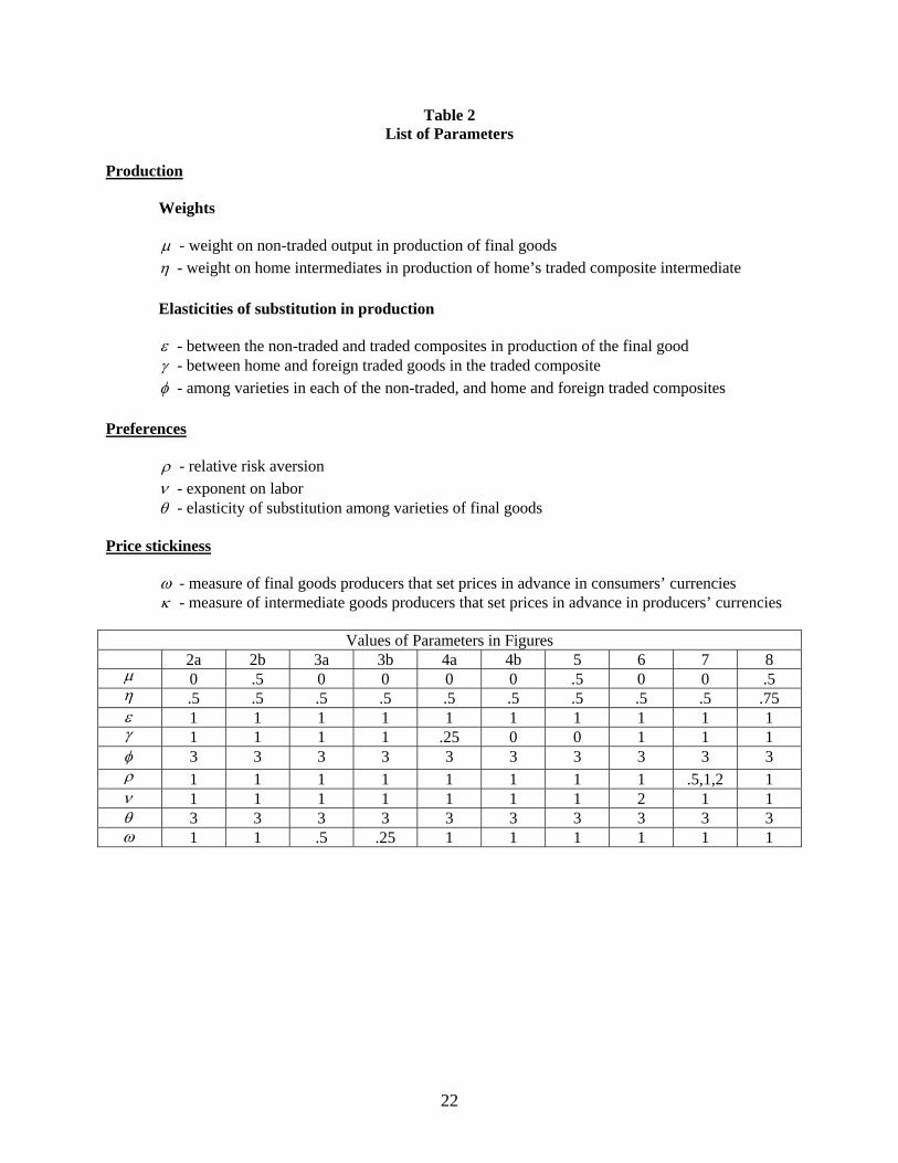
Table 2 List of Parameters

Production Weights µ - weight on non-traded output in production of final goods η - weight on home intermediates in production of home’s traded composite intermediate Elasticities of substitution in production ε - between the non-traded and traded composites in production of the final good γ - between home and foreign traded goods in the traded composite φ - among varieties in each of the non-traded, and home and foreign traded composites Preferences ρ - relative risk aversion ν - exponent on labor θ - elasticity of substitution among varieties of final goods Price stickiness ω - measure of final goods producers that set prices in advance in consumers’ currencies - measure of intermediate goods producers that set prices in advance in producers’ currencies κ

Values of Parameters in Figures 2a 2b 3a 3b 4a 4b 5 6 7 8

µ 0 .5 0 0 0 0 .5 0 0 .5 η .5 .5 .5 .5 .5 .5 .5 .5 .5 .75 ε 1 1 1 1 1 1 1 1 1 1 γ 1 1 1 1 .25 0 0 1 1 1 φ 3 3 3 3 3 3 3 3 3 3 ρ 1 1 1 1 1 1 1 1 .5,1,2 1 ν 1 1 1 1 1 1 1 2 1 1 θ 3 3 3 3 3 3 3 3 3 3 ω 1 1 .5 .25 1 1 1 1 1 1

22

Home intermediate producing households Home final good consumers

Foreign intermediate producing households Foreign final good consumers

Home assembly firms in N, H, F composite goods

Foreign assembly firms in N*, H*, F* composite goods

Home final goods firms Foreign final goods firms

Figure 1 Flow chart for the model

23

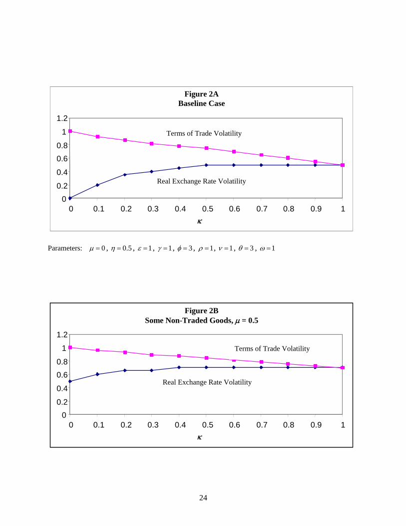
Figure 2A Baseline Case

00.2

0.4

0.60.8

1

1.2

0 0.1 0.2 0.3 0.4

Terms of Trade Volatility

Real Excha

Parameters: 0µ = , 0.5η = , 1ε = , 1γ = , 3φ =

Fi

Some Non-Tr

00.2

0.4

0.60.8

1

1.2

0 0.1 0.2 0.3 0.4

Real Exch

0.5 0.6 0.7 0.8 0.9 1κ

nge Rate Volatility

, 1ρ = , 1ν = , 3θ = , 1ω =

gure 2B aded Goods, µ = 0.5

0κ

ange

24

.5 0.6 0.7 0.8 0.9 1

Terms of Trade Volatility

Rate Volatility

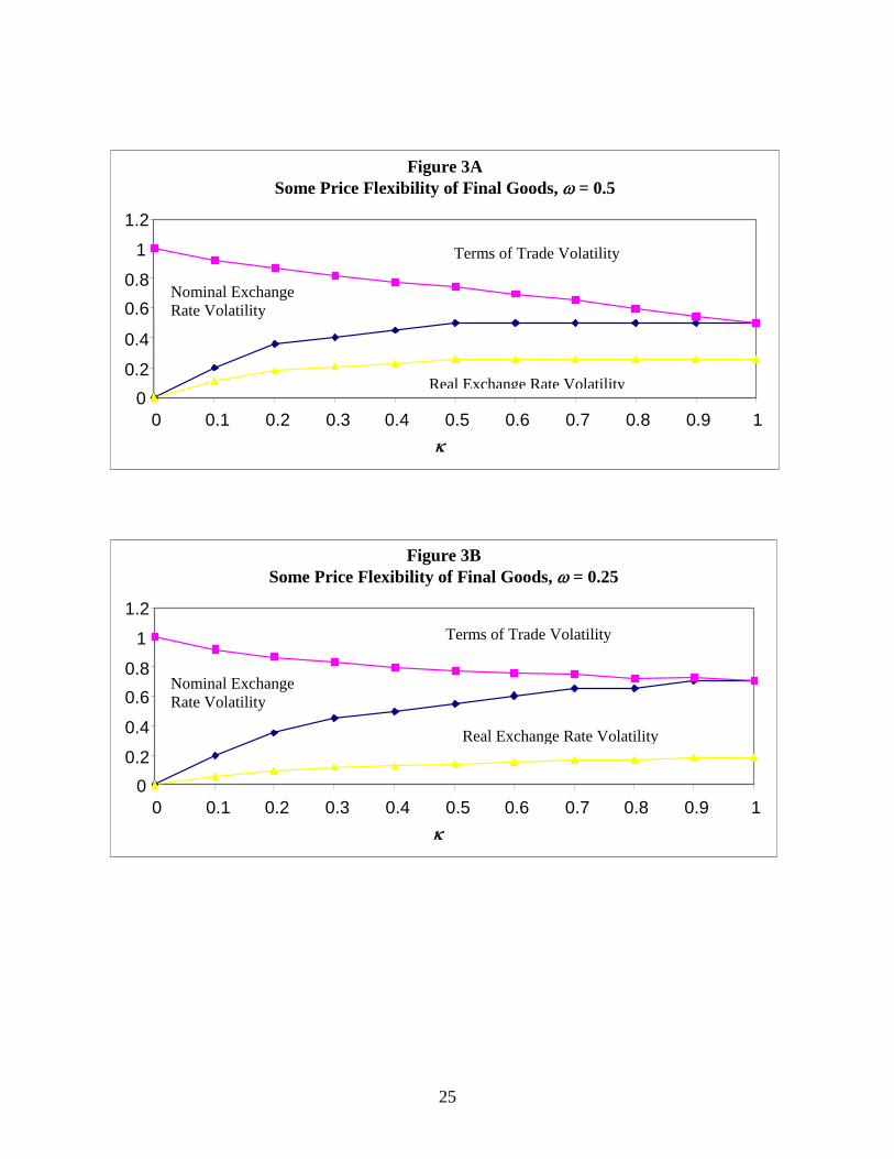
Figure 3A Some Price Flexibility of Final Goods, ω = 0.5

00.2

0.4

0.60.8

1

1.2

0 0.1 0.2 0.3 0.4 0.5 0.6 0.7 0.8 0.9 1κ

Terms of Trade Volatility

Nominal Exchange Rate Volatility

Real Exchange Rate Volatility

Figure 3B

Some Price Flexibility of Final Goods, ω = 0.25

0

0.2

0.4

0.60.8

1

1.2

0 0.1 0.2 0.3 0.4 0.5 0.6κ

Terms of Tra

Nominal Exchange Rate Volatility

Real Exch

25

0.7 0.8 0.9 1

de Volatility

ange Rate Volatility

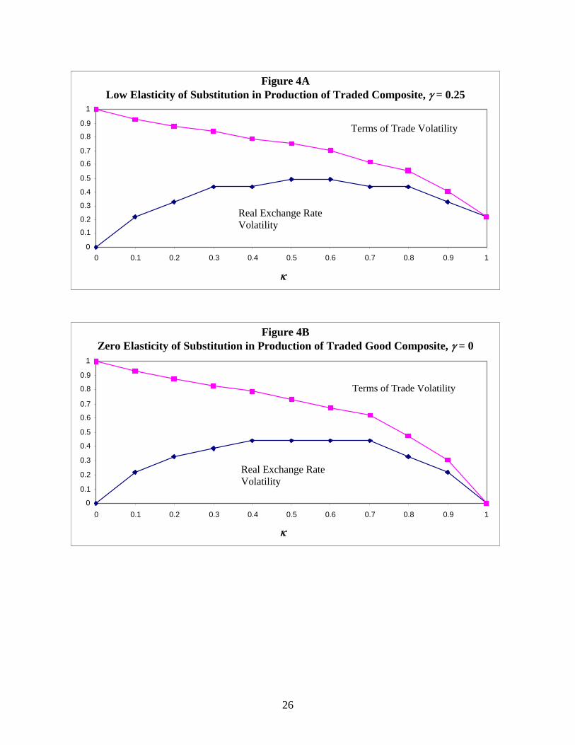
Figure 4A Low Elasticity of Substitution in Production of Traded Composite, γ = 0.25

0 0.1

0.2

0.3

0.4

0.5

0.6

0.7

0.8

0.9

1

0 0.1 0.2 0.3 0.4 0.5 0.6 0.7 0.8 0.9 1

κ

Terms of Trade Volatility

Real Exchange Rate Volatility

Figure 4B

Zero Elasticity of Substitution in Production of Traded Good Composite, γ = 0

0 0.1

0.2

0.3

0.4

0.5

0.6

0.7

0.8

0.9

1

0 0.1 0.2 0.3 0.4 0.5 0.6 0.7 0.8 0.9 1

κ

Terms of Trade Volatility

Real Exchange Rate Volatility

26

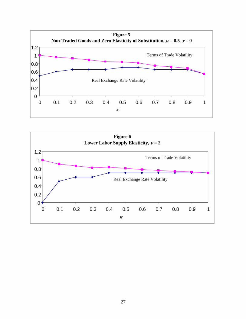
Figure 5

Non-Traded Goods and Zero Elasticity of Substitution, µ = 0.5, γ = 0

0

0.2

0.4

0.60.8

1

1.2

0 0.1 0.2 0.3 0.4 0.5 0.6 0.7 0.8 0.9 1κ

Terms of Trade Volatility

Real Exchange Rate Volatility

Figure 6 Lower Labor Supply Elasticity, ν = 2

00.2

0.4

0.60.8

1

1.2

0 0.1 0.2 0.3 0.4 0.5 0.6 0.7 0.8 0.9 1κ

Terms of Trade Volatility

Real Exchange Rate Volatility

27

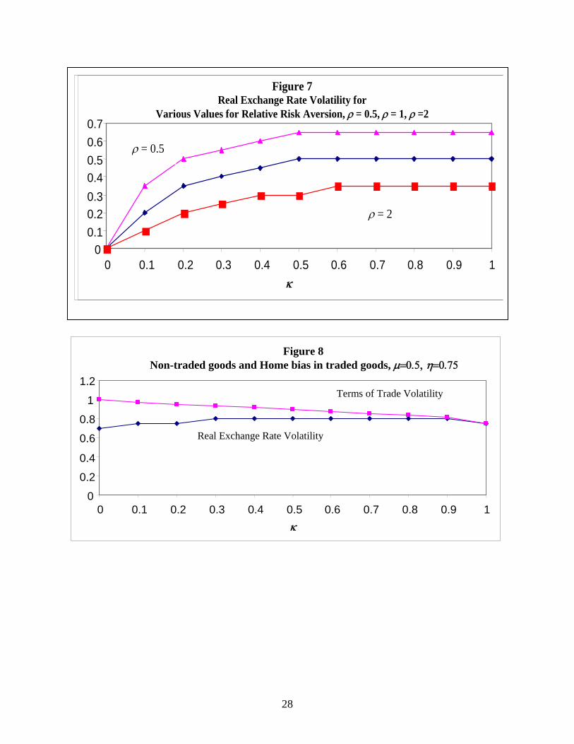
Figure 7 Real Exchange Rate Volatility for

Various Values for Relative Risk Aversion, ρ = 0.5, ρ = 1, ρ =2

00.10.20.30.40.50.60.7

0 0.1 0.2 0.3 0.4 0.5 0.6 0.7 0.8 0.9 1κ

ρ = 0.5

ρ = 2

Figure 8 Non-traded goods and Home bias in traded goods, µ=0.5, η=0.75

1.2

0

0.2

0.4

0.6

0.8

1

0 0.1 0.2 0.3 0.4 0.5 0.6 0.7 0.8 0.9 1κ

Terms of Trade Volatility

Real Exchange Rate Volatility

28

Appendix A. Derivation of conditions in Table 1

The consumption index, C, from equation (1) is given by:

(A1) 1 11

0( )C C j dj

θθ θθ− −⎡ ⎤

= ⎢ ⎥⎣ ⎦∫ , 1θ > ,

where is the consumption of variety j. The aggregate price index is then given by: ( )C j

1

1 11

0( )P P j dj θθ −−⎡ ⎤= ⎢ ⎥⎣ ⎦∫ .

Minimizing subject to (A1), and using the equilibrium condition gives

demand for the firm’s product:

1

0( ) ( )P j Y j dj∫ ( ) ( )C j Y j=

(A2) ( )( ) P jY j CP

θ−⎡ ⎤= ⎢ ⎥⎣ ⎦

.

Aggregate profits of home final goods firms are given by , where is defined

by

1

0( )j djΠ = Π∫ ( )jΠ

( ) ( ) ( ) ( , ) ( )F FH Tj P j Y j c P P Y jσ τΠ = − − , and the subsidy and taxes satisfy

1F θσ

θ=

−, and

(recall that subsidies are chosen to offset monopoly pricing distortions, and taxes are

used to finance the subsidies).

( 1)F F PCτ σ= −

Profit maximization for the final goods firm, subject to (A2), in face of the optimal subsidy, gives

equation (5) of Table 1.

Minimizing subject to (2) gives the demand function for each intermediate

aggregate. For example, the demand for the home non-traded intermediate aggregate (by firm j) is:

( ) ( )H H T TP Y j P Y j+

(A3) 11 1 1

( ) ( )( (1 ) )

HN

H T

PY j Y jP P

ε

ε ε ε

ηµ µ

−

− − −

⎛ ⎞⎜ ⎟= ⎜ ⎟⎜ ⎟+ −⎝ ⎠

,

Here ( )1

1 11

0( )HP P j dj φφ −−= ∫ is the price index for the home non-traded intermediate aggregate supplied by

assembly firms in the home non-traded sector, and ( )( )1

1 11 *(1 )T H FP P SPγ γγη η

− −−= + − is the price index of

the traded intermediate aggregate, where HP is the price index for the home intermediate composite

which goes into the home traded aggregate. It follows then that the demand by final good firm j for the

home component of the traded intermediate aggregate is:

1

(A4) 11 * 1 1

( ) ( )( (1 )( ) )

HHT T

H F

PY j Y jP SP

γ

γ γ γ

ηη η

−

− − −

⎛ ⎞⎜ ⎟= ⎜ ⎟⎜ ⎟+ −⎝ ⎠

.

Because all home intermediate goods have identical production technologies, the price index is the

same as that of the non-traded intermediate aggregate.

HP

*FP is the price index for the foreign intermediate

composite. Assembly firms purchase intermediates directly from the intermediate producing households and

supply them competitively to final goods firms. For instance, assembly firm j supplying the non-traded

intermediate aggregate minimizes subject to 1

0( ) ( , )H NP i Y i j di∫

1 11

0( ) ( , )N NY j Y i j di

φφ φφ− −⎡ ⎤

= ⎢ ⎥⎢ ⎥⎣ ⎦∫ , which gives

demand for the (non-traded) home intermediate good i by firm j:

(A5) ( )( , ) ( )HN N

H

P iY i j Y jP

φ−⎡ ⎤

= ⎢ ⎥⎣ ⎦

.

A similar condition applies to the demand for the traded intermediate goods, and for the foreign traded

intermediate good.

Households i’s budget constraint under complete markets is given by

(A6) , ( ) ( , ) ( , ) ( , ) ( ) ( , )IHP z C i z P i z L i z z B i zσ τ= + +

where the z index refers to the state (and, as previously, i to the household) , and 11

I φσφ

= >−

, with

lump sum taxes . ( 1)IHP Lτ σ= − ( , )B i z is household i’s holdings of bonds that pay off in state z. The

market for state contingent bonds is open prior to the realization of shocks. Home households are

endowed with ownership of all domestic final goods firms. State contingent claims are chosen subject to

the constraint that the value of all claims, ( ) ( , )zq z B i z∑ , equals the initial value of firms.

The first order conditions for the household i’s choice of state contingent consumption and price,

given the demand for household i’s good from (A3) above, are given by:

(A7) ( , ) ( ) ( )C i z q z P zρ λ− =

(A8) ( , ) ( ) ( , )( 1)( , )

vI

H

KL i z q z L i zP i z

φ λ σ φ= −

Putting these two equations together, and imposing symmetry, so that all households in the home country

set identical prices of intermediates, gives equation (7) in Table 1. Equation (8) is obtained by using the

identical equation to (A7) for the foreign country, along with the assumption of ex ante equality, so that

the Lagrange multipliers are identical across the two countries. Finally, the market clearing equation for

2

traded goods (9) is obtained by using (A2) and (A4), aggregated across goods, again using the symmetry

assumption that all home final goods prices are equal, and all home intermediate goods prices are equal.

The condition (10) for non-traded goods uses (A2) and (A3) in the same way. Condition (12) in Table 1

is just the assumed monetary policy rule.

Appendix B. Proof of Propositions

Proof of Proposition 1

Using the monetary policies (20) in equation (7) and its foreign counterpart, we get

(B1) HP KP CP

ρ⎛ ⎞

= ⎜ ⎟⎝ ⎠

(B2) *

* * **FP K P C

P

ρ⎛ ⎞

= ⎜ ⎟⎝ ⎠

Now using equations (B1) and (B2) to construct ( )1

1 11 1 * (1 ) 1(1 ) (1 )( )H H FP P SP

ε εε γ γ γµ µ η η

− −− − − −

⎛ ⎞+ − + −⎜ ⎟

⎝ ⎠ , which

is the marginal cost expression for final goods firms. With the definitions of τ and , we can establish

that

C

( )1

1 11 1 * (1 ) 1(1 ) (1 )( )H H FP P SP

ε εε γ γ γµ µ η η

− −− − − −

⎛ ⎞+ − + −⎜

⎝ ⎠⎟ is state independent. This implies from (5’) and its

foreign counterpart that final goods prices are set at their ex-ante optimal levels. Since then the equations

of Table 1 hold exactly, the monetary policy rules of Proposition 1, consumption and employment must

be at their flexible price levels given that the terms of trade is equal to its flexible price level. From the

pricing equations again, we can establish that the equilibrium pre-set prices satisfy . * *,P P= =

Proof of Proposition 2

Substituting the monetary rules (22) into condition (7’), we find that

(B3) HP = .

Hence, the optimal intermediate good price is state independent. Equivalently, if we substitute (22) into

(7), we get the same answer as (B3). Hence, even with sticky intermediate goods prices, (7) holds exactly

as in Table 1. A similar condition holds for the foreign intermediate good price. Therefore, the solutions

of the flexible price economy apply. In this case, the exchange rate adjusts to as to replicate the flexible

price terms of trade. Nominal price levels follow from (B3), its foreign equivalent, and the pricing

equations for final goods in each country.

Proof of Proposition 3.

From (8) in the case where 0µ = and 0.5η = , with the monetary policies (24), given that P and

are predetermined, the exchange rate is predetermined. With fixed proportions, and given that , *P HP

3

*FP , and S are predetermined, condition (5’) becomes *1 (

2 H FP P SP= + ) . The market clearing condition

becomes . Hence, the monetary policies ensure that PPP holds (since all terms in the final goods

pricing relationship are predetermined) and there is efficient risk sharing. Employment is also equalized

across countries. The level of employment is determined from the monetary policies such that

L C=

FPL C CP

= = . From condition (7’), and the analogous condition for the foreign country, added

together, we get

(B4)

*

*

1

( )( )21

2H F

K KE LP SPP EL ρ−

++

= =

Substitute in (B4) for L and FPC as defined in (23), it follows immediately that P = (and *P *= ), so

that consumption and employment are at the flexible price equilibrium levels.

4