NBER WORKING PAPER SERIES

DO THE RICH FLEE FROM HIGH STATE TAXES?EVIDENCE FROM FEDERAL ESTATE TAX RETURNS

Jon BakijaJoel Slemrod

Working Paper 10645http://www.nber.org/papers/w10645

NATIONAL BUREAU OF ECONOMIC RESEARCH1050 Massachusetts Avenue

Cambridge, MA 02138July 2004

The views expressed herein are those of the author(s) and not necessarily those of the National Bureau ofEconomic Research.

©2004 by Jon Bakija and Joel Slemrod. All rights reserved. Short sections of text, not to exceed twoparagraphs, may be quoted without explicit permission provided that full credit, including © notice, is givento the source.

Do the Rich Flee from High State Taxes? Evidence from Federal Estate Tax ReturnsJon Bakija and Joel SlemrodNBER Working Paper No. 10645July 2004JEL No. H23, H71, H73, H77, R23, J14

ABSTRACT

This paper examines how changes in state tax policy affect the number of federal estate tax returns

filed in each state, utilizing data on federal estate tax return filings by state and wealth class for 18

years between 1965 and 1998. Controlling for state- and wealth-class specific fixed effects, we find

that high state inheritance and estate taxes and sales taxes have statistically significant, but modest,

negative impacts on the number of federal estate tax returns filed in a state. High personal income

tax and property tax burdens are also found to have negative effects, but these results are somewhat

sensitive to alternative specifications. This evidence is consistent with the notion that wealthy

elderly people change their real (or reported) state of residence to avoid high state taxes, although

it could partly reflect other modes of tax avoidance as well. We discuss the implications for the

debate over whether individual states should “decouple” their estate taxes from federal law, which

would retain the state tax even as the federal credit for such taxes is eliminated. Our results suggest

that migration and other observationally equivalent avoidance activities in response to such a tax

would cause revenue losses and deadweight losses, but that these would not be large relative to the

revenue raised by the tax.

Jon BakijaDepartment of EconomicsWilliams College Williamstown, MA 01267jbakija@williams.edu

Joel SlemrodUniversity of Michigan Business School701 Tappan Street, Room A2120Ann Arbor, MI 48109-1234and NBERjslemrod@umich.edu

1

Introduction

This paper presents evidence on the degree to which wealthy elderly people migrate or

otherwise undertake actions to avoid state taxes, based on an examination of the

relationship between changes in state tax policies and changes in the number of federal

estate tax returns filed in each state over time. In setting optimal state tax policy,

particularly with regards to the degree of progressivity, the extent to which people flee

states that attempt to impose relatively high tax burdens on them is a critical

consideration. A long-standing argument in the public finance literature holds that state

governments should refrain from redistributive tax and transfer policies, and that these

should instead be the responsibility of the central government (Musgrave, 1959, and

Oates, 1972). Out-migration by high-income people and in-migration by low-income

people may partly or fully undermine a state’s effort to achieve redistribution, and the

deadweight losses arising from distorted location decisions might be avoided if the same

redistribution were instead effected by the central government. Yet we observe that states

do indeed implement policies such as progressive income taxes and wealth-transfer taxes,

as well as redistributive spending policies. Possible explanations might include a limited

willingness of individuals to migrate across states in response to taxes, which prevents

the impact of progressive state policies from being completely undone, coupled with

heterogeneity across states in tastes for redistribution, and the possibility that

redistribution is a local public good.2 When states do operate redistributive policies, the

optimal degree of redistribution from the state’s perspective is a declining function of the

degree of mobility in response to taxes (Mirrlees, 1982).3 An extensive empirical

literature has developed to examine whether the migration decisions of the poor are

affected by the generosity of state anti-poverty policies, usually finding little evidence of

an effect.4 But to date, we have little or no information on whether progressive state tax

policies are affecting the location decisions of the rich.5

Recently, the question of whether rich elderly people in particular flee from states

that tax them relatively heavily has become an especially salient question for state

governments. States must now decide how to respond to the elimination of a credit in the

federal estate tax for state estate and inheritance (henceforth “EI”) tax payments. In the

2

recent past, all states imposed a tax at death to “soak up” the maximum available federal

credit. A soak-up tax imposed no incremental burden on a state’s residents, but rather

merely effected a transfer of revenue from federal to state governments. The Economic

Growth and Tax Relief Reconciliation Act of 2001 (EGTRRA) scheduled a gradual

elimination of the credit for state EI taxes between 2002 and 2004, after which it will be

replaced by a deduction.6 When the federal credit is eliminated, states that maintain their

estate taxes at the former soak-up level will be imposing larger incremental burdens than

states that do not. By 2006, the difference in tax burdens on estates larger than $675,000

between a state that maintains the tax in its 2001 form, versus a state that eliminates the

tax, will be on average roughly 4.5 percent of the bequest.7 As of January 2004, eighteen

states that formerly levied soak-up estate taxes had “decoupled” from federal law, so that

they would persist at pre-EGTRRA levels even as the federal credit is eliminated. 8

Numerous other states were debating whether to take legislative action to decouple their

estate taxes, while states with taxes that were already decoupled were debating whether to

eliminate them. The potential impact of such taxes on migration behavior is at the crux of

the debate over this issue.

Substantial historical variation in state tax policy offers an opportunity to learn

about how tax burdens on the rich affect their location decisions. EI taxes provide a

particularly good experiment. Historically, most states imposed their own idiosyncratic

EI taxes and also operated a soak-up tax in parallel, so that tax liability at death would

equal the larger of the two taxes. When the state’s idiosyncratic EI tax exceeded the soak-

up tax liability, the excess was an incremental burden relative to other states. But,

beginning in the 1970s, more and more states began to eliminate these taxes, switching to

sole reliance on the soak-up tax. The timing of repeal varied greatly across states; for

example, 28 states repealed their idiosyncratic EI taxes between 1976 and 2000, and the

timing of those changes was spread fairly evenly throughout the period (Conway and

Rork, 2004a). Other states consistently imposed no incremental EI tax over this period, or

maintained a tax throughout the period. Differences across states in effective income,

sales, and property tax burdens exhibited less stark, but still substantial, variation over

time. For example, the elimination of deductibility of sales taxes in the Tax Reform Act

of 1986 made states with high sales taxes become relatively less attractive compared to

3

other states, and various state income tax reforms had modest effects on the degree of

progressivity. Historical tax law changes thus arguably provide treatment and control

groups for testing how differing time patterns of tax burdens across states match up with

time patterns in the number of estate tax return filers claiming residence in each state.

Some recent research has examined the determinants of migration behavior for

the elderly in general. None, though, has focused on the wealthy elderly, who are now

almost exclusively the ones impacted by state EI taxes, and whose behavior might have

special implications for the optimal progressivity of a state tax system. Conway and

Houtenville (2001) review the previous literature, and then examine migration flows

between each pair of states in the U.S. between 1985 and 1990, using aggregate state-

level data from the 1990 U.S. Census. They find some evidence that the elderly in general

are less likely to migrate into states with higher EI taxes, although they also find the

perverse result that the elderly are less likely to migrate out of states with higher EI taxes.

Results for other types of taxes are rather mixed and sensitive to the specification chosen.

Duncombe, Robbins, and Wolf (2003) estimate a discrete choice model of county-to-

county migration decisions of the elderly between 1985 and 1990, again using 1990

Census data. They find that various taxes, including inheritance taxes, reduce the

probability of locating in a jurisdiction, although estate tax rates are found to have a

positive effect on the probability of locating in a state. Using the Health and Retirement

Survey, Farnham and Sevak (2004) examine whether members of “empty nest”

houesholds, who would presumably prefer to move to jurisdictions with lower property

taxes and education spending, actually reduce their property tax burdens when they

move. They find that when such people move across state boundaries they achieve some

modest property tax reduction, but not when they move within-state. Conway and Rork

(2004b) recently undertook the first study to utilize a panel data approach to study

aggregate migration flows, controlling for time-invariant unobservable characteristics of

states with state-specific fixed-effects. Based on 1970 through 2000 decennial census

data, they examine how aggregate in-migration and out-migration flows of states change

over time in response to changes in state taxes, and again find mixed results.

A common feature of all of these previous studies (with the exception of Farnham

and Sevak, which only examined property taxes) is that the measures of state tax burdens

4

have been rough approximations. Some studies use measures based on aggregate tax

collections, in spite of the fact that these measures are endogenously related to migration

behavior.9 In other cases, studies apply “representative” tax parameters that are assumed

to apply equally to all taxpayers in a state, despite the fact that the burdens of EI and

income taxes are extremely heterogeneous across individuals. We would expect that,

ceteris paribus, states imposing taxes that are relatively progressive compared to other

states would tend to repel those who are relatively heavily taxed and attract those who are

relatively lightly taxed. In that case, it may not be very informative to examine how

migration responds to a tax rate that is calculated, for example, at a single

“representative” level of wealth or income for the state as a whole.10 Because EI taxes in

particular are so heavily concentrated on the wealthy, their effects may be lost in studies

relying on aggregate data or using representative tax rates that are assumed to apply to

all.

Our study addresses the question of how the reported locations of wealthy elderly

people respond to state tax policy by utilizing panel data on the number of federal estate

tax returns filed in each of five wealth classes in each state for 18 years between 1965

and 1998. A distinct advantage of using federal estate tax return data is that this is the

only kind of data available providing information on any significant number of wealthy

people and their locations.11 A disadvantage is that, in contrast to the data typically used

in the migration literature, we do not actually observe whether an individual moves, only

his or her reported state of residence at the date of death. There are some factors, such as

tax-induced changes in wealth accumulation behavior, or undertaking avoidance

activities that enable one to “pretend” to move, that are difficult to distinguish from

migration in our data. As such, our approach is similar to the extensive literature on the

elasticity of taxable income, where we have compelling evidence that some sort of tax

avoidance behavior with important policy implications is occurring, but we cannot be

absolutely certain of its exact form.12

We model the choice of (reported) state of residence in both linear regression and

conditional logit frameworks, and we take advantage of the state panel characteristic of

our data to control for state- and wealth-class specific fixed-effects and state-specific time

trends, in addition to controlling for a broad array of time-varying state characteristics.

5

We thus take a “difference-in-differences” type approach, where the identification for the

tax effects comes entirely from differences across states in the time pattern of tax rates

within each wealth class. A major contribution of our work is the development and use of

detailed federal and state inheritance, estate, and income tax calculators that allow us to

construct accurate estimates of the tax burdens likely to apply to the individuals in our

study in different states and at different wealth levels.

We find that, controlling for state and wealth class fixed effects, a one percentage

point increase in the wealth-class-specific effective state EI average tax rate is associated

with 1.4 percent to 2.7 percent decline in the number of federal estate tax returns filed in

the state, depending on the specification. Estates over $5 million are found to be

particularly sensitive to the EI tax, declining by nearly 4 percent in response to a one-

percentage point rate increase. Sales tax, income tax, and property tax rates are also

found to have similar and sometimes larger negative impacts on the number of federal

estate tax returns filed in a state, although the results for the latter two taxes are sensitive

to alternative specifications. Controlling for unobserved heterogeneity in state

characteristics has an important effect on the estimates, in the direction of increasing the

estimated magnitude of the negative impact of taxes. At the end of the paper, we consider

what our estimates imply about the debate over state EI taxes, and what they contribute to

our understanding of the welfare costs of state taxation. Our results support the idea that

state governments face a trade-off and should take tax-induced migration and related

avoidance activities into account when setting tax policy. But our results also imply that

in the case of a decoupled estate tax, revenue losses and deadweight losses from these

particular forms of behavioral response are unlikely to be large relative to revenues

collected

Estate Tax Return Data

We begin with a description of the federal estate tax return data that forms the basis of

our study, as an understanding of the data helps explain the choices we have made in our

econometric approach. The federal estate tax is a tax on the total value of bequests made

at death, less deductions for bequests to a spouse, bequests to charity, and a few other

6

miscellaneous items. It applies exclusively to estates that exceed an exemption level ($1.5

million in 2004) that is effectively created by a “unified credit.” A return is required on

behalf of any decedent whose “gross estate” (assets before subtracting debts or

deductions) exceeds the exemption level. Above the exempt level, substantial marginal

tax rates are imposed, ranging from 45 to 48 percent in 2004. The exemption level has

fluctuated significantly in value over time. In nominal terms, the exempt level was

$60,000 from 1954 to 1976, after which it increased in steps to $600,000 by 1987, where

it stayed until 1997 before beginning to increase again.13

Our empirical analysis is based on tabulations of federal estate tax return data

provided to us by the Statistics of Income division of the Internal Revenue Service (IRS).

The underlying data set is a sample of returns stratified based on size of gross estate, age

at death, and either year of death (1985 and after) or filing year (before 1985).14 The

average sampling rate for the observations we use was about 25 percent of the national

population of estate tax returns, although this varies widely from year to year. To

preserve confidentiality, the data were provided to us in the form of aggregated cells,

broken up into year, state, and wealth class combinations. We use 18 years of data --

1965, 1969, 1976, 1982, and 1985 through 1998. The data for 1985-1998 are arranged by

year of death. Data before 1985 represent estate tax returns that were filed in the

following year; most of these returns pertain to deaths that occurred in the year indicated.

The missing years are omitted either because the IRS did not draw a sample of returns

filed in the following year, or because a key piece of information such as state of

residence was not collected. All 50 states are included in all years, and the District of

Columbia is included starting in 1976. The wealth classes are defined based on net worth,

which equals the total gross estate minus debts.15 The wealth categories (measured in

constant 1996 dollars, calculated using the CPI-U) are $400,000 - $750,000, $750,000 -

$1.25 million, $1.25 million - $2 million, $2 million - $5 million, and over $5 million. To

maintain comparability of populations within similar cells across years, we omit any

wealth category in any particular year where the federal filing threshold was above the

minimum bound of the category.16 For each year-wealth-state cell, we have information

on the number of sampled returns in that cell, as well as an estimate of the number of

population estate tax returns represented by those sampled observations (the population

7

estimate is the weighted sum of sampled returns, where each weight is the inverse of the

known sampling probability for that observation). If the number of returns in the cell was

between 1 and 3, it was reported to us as 2, so that we would not be able to identify the

characteristics of any particular individual. The number of state-wealth-year cells

included in the analysis is 3,713, the number of underlying sampled returns is 236,829,

and the estimated population of returns represented is 955,987. Thus, the average number

of sampled returns in a cell is 64, and the average number of population returns

represented by a cell is 257. In 43 of the cells, or 1.1 percent, there were no sampled

returns, and in 286 cells, or 7.7 percent, there were between 1 and 3 sampled returns.

Theory and Empirical Approach

Our empirical approach to estimating how state characteristics and policy variables

influence the location of federal estate tax return filers derives directly from a simple

model in which elderly individuals make decisions about where to live based on

comparison of the utilities they would obtain at each location. To be precise, consider an

individual i who has a Cobb-Douglas utility function over consumption (C), and the

inheritance received by heirs (I).17 The utility (U) and budget constraints associated with

choosing to live in state j can be represented as:

(1) Uij = Cijα1Iij

α2exp(δ’Zij + εij)

Cij = Wij – Bij - TLij

Iij = Bij - TEij

In this formulation Wij is wealth, Bij is the bequest gross of taxes, TEij is the estate and

inheritance tax liability imposed on bequests, TLij is the tax liability associated with

location j while alive, Zij is a vector of state-specific amenities and characteristics that we

will consider in detail later, and εij is a random error reflecting heterogeneity in tastes.

Substituting in for C and I, taking logs of both sides, and taking a first-order Taylor-series

approximation of ln(C) and ln(I) around C = (W-B*) and I = B*, respectively (where *

indicates the optimal value), in order to separate out the effects of taxes, yields:

8

(2) ln(U*ij) = α1ln(Wij – B*ij) + α2ln(B*ij) - α1τLij - α2τE

ij + δ’Zi1 + εij

where τLij = Tij

L / (Wi – B*ij) is the average tax rate while alive (expressed as a share of

expenditures while alive gross of taxes, since that is the point around which we are taking

the approximation), and τEij = Tij

E / B*ij is the average estate and inheritance tax rate

(expressed as a share of the pre-tax bequest),

When deciding whether to live in a specific state j=1 or an alternative state j=2,

state 1 is selected if utility in state 1 exceeds utility in state 2, that is if:

(3) α1 [ln(Wi – B*i1)-ln(Wi – B*i2)] + α2 [ln(B*i1) - ln(B*i2)]

- α1 [τLi1 - τL

i2] - α2 [τEi1 - τE

i2] + δ’[Zi1-Zi2] + (εi1 - εi2) > 0

If εij is drawn from a logistic distribution, then the effects of the explanatory

variables on the probability of choosing state j can be estimated with a logit model. If we

generalize to a choice among a large number of states (50 plus the District of Columbia in

our study), then the probability Pi1 that individual i is observed in location j=1 is given

by:

(4) Pi1 = exp(β’Xi1)/Σj[exp(β’Xij)],

where β’Xij is the non-error part of the right-hand-side of equation (2) above. Estimation

proceeds by finding the vector of parameters β that maximizes the probability that the

individuals in the sample choose their observed locations. This is the “conditional logit”

model developed by McFadden (1974).18 It is sometimes called a “fixed effects” logit,

because it has the useful feature that any individual characteristics or aggregate

influences that are constant across locations are effectively differenced out of equation

(4) -- they cancel out because they affect all of the exp(.) terms equally. So, for example,

any aggregate influences that would normally be controlled for through year fixed effects

in a linear regression are automatically controlled for in conditional logit, as they are

constant across j and thus difference out. For our conditional logit estimates, we treat

9

each of the 236,829 sampled returns in our data as an independent observation making a

choice from among all of the available jurisdictions, based on representative tax rates that

someone in his or her particular wealth class would face in each state in that year, and the

characteristics of each of the states.19 Our data do not provide us with individual-level

characteristics, but to the extent that unobserved individual characteristics are the same

regardless of which state is chosen, they are irrelevant in the conditional logit.20 The

information we do have varies only across wealth classes (which we will denote through

the subscript k), states (j), and years of death (t), so the ij subscripts in equation (4) are

replaced with jkt subscripts in our empirical analysis.

We also use a simpler approach derived from the same theoretical model that

allows us to estimate a linear regression. If we treat the choice about whether to live in a

particular state j as a choice between that state and a single alternative option with

characteristics that are a composite of the rest of the nation as a whole, and again assume

logistically distributed errors, then the probability Pjkt that an individual in wealth class k

and year t will choose state j is:

(5) Pjkt = exp[β’(Xjkt-X~j,kt)]/{1+exp[β’(Xjkt-X~j,kt)]},

where X~j,kt is a vector of representative values of the characteristics in X for the rest of

the nation as a whole (excluding state j) for that wealth class and year.21 This can be

rearranged into a linear equation:

(6) ln[Pjkt/(1-Pjkt)] = β’(Xjkt-X~j,kt)

Pjkt represents the proportion of nationwide returns in wealth class k and year t that are

filed in state j (i.e., the observed probability of choosing j). This is a common approach

for dealing with aggregated data like ours that provides information on the proportion of

people in a cell who make a particular choice. The dependent variable is known as the

log-odds ratio, and the interpretation of the coefficients is the same as in the conditional

logit – in both cases each coefficient represents the marginal effect of an explanatory

variable on the log-odds ratio. In this approach, the unit of analysis is the state-wealth-

10

year cell, so there are 3,713 separate observations in the regression. As Greene (2000, pp.

834-837) notes, this kind of regression exhibits heteroskedasticity of a known form, and

we deal with this appropriately through weighted least squares.22 As with the conditional

logit, individual characteristics that are constant across states, as well as any aggregate

influences that have a similar proportional effect on the number of estate tax returns filed

in all states, difference out of equation (7), and so we are effectively controlling for them.

One matter of interpretation in both approaches is that if the optimal bequest B*ij

is assumed to be constant across states, then the first two terms in equation (3) above

(which form the basis of the linear model) are zero, and the first two terms in equation (2)

cancel out of the conditional logit likelihood function, so we are left with tax rates and

the state characteristics contained in Z as the only explanatory variables. However,

B*ij may vary systematically across states, because the income and substitution effects of

state tax policies may lead to different optimal choices regarding things like wealth

accumulation and avoidance behavior across the different states. In that case, if our goal

were to measure α1 and α2, then B*ij would have to enter our estimation equations to the

extent that it differs across states. It is, though, clearly impossible to observe what an

individual’s optimal B* would be in each of the 51 possible jurisdictions, so the first two

terms in equation (2) (for the conditional logit) and (3) (for the linear regression) will be

omitted variables. The implication is that the coefficients on the tax rate variables do not

directly measure the α1 and α2 parameters of the utility function (which only reflect the

direct effect of taxes on utility arising because they reduce after-tax consumption and

inheritances). Rather, the tax coefficients will now reflect the net effect of taxes on utility

after taking into account the fact that individuals can offset some of the negative impact

of state taxes by re-optimizing their choices regarding consumption and bequests.

Tax and Government Spending Variables

In this section, we explain some essential features of state EI taxation, describe the

construction of our fiscal variables, and provide information on how the time-series

variation in the tax variables differs across states, to illustrate the sources of identification

for our estimates. 23 Although the theory above was developed in terms of a total average

11

tax rate in life and at death, in the empirical analysis we include a separate tax rate for

each major type of tax (EI, income, sales, and property) because each one may have a

different effect on location decisions.

As noted above, the federal estate tax has long provided a limited credit to the

taxpayer for EI taxes paid to state governments, and this credit has a critical impact on

the degree of variation in relative tax burdens across states. The credit was initially

introduced in 1924, and the maximum allowable credit has always been an increasing

function of the size of the taxable estate; the schedule that applied from 1954 through

2001 is shown in Table 1. Because the federal credit for state taxes was non-refundable,

the maximum allowable credit was actually the minimum of the amount determined

through Table 1, and federal estate tax liability calculated before application of the credit

for state taxes.24 If a state were to cut its EI tax below the maximum federal credit, the

reduction in state tax would be exactly offset by an increase in federal tax, making

residents of the state no better off while transferring revenue from state to federal coffers.

As a result, all states eventually implemented an estate tax provision that “soaked up” any

otherwise unused federal credit.25 Historically, most states also operated their own

idiosyncratic estate and/or inheritance tax systems in addition to the soak-up provision. In

those cases, the decedent’s tax payment to the state would be the larger of the liability

under the state’s unique EI tax and the liability under the soak-up tax. Some states, on

the other hand, did not operate their own special EI taxes, and instead relied solely on a

soak-up tax exactly equal to the maximum allowable federal credit; these states imposed

no positive incremental EI tax burden. Over the last four decades, more and more states

gradually repealed their own idiosyncratic EI taxes, and switched to relying exclusively

on the soak-up tax.

To represent the incremental state EI average tax rate in each state, year, and

wealth class, we construct a variable EIATR, which is defined as the combined federal-

state inheritance and estate tax liability as a share of net worth, less what it would be in a

state relying exclusively on the soak-up tax. It is based on the federal and state tax rules

in effect for deaths on July 1 of the relevant year. In constructing this variable we have to

address the fact that in some cases the tax burden can vary depending on how the estate

was divided up among various types of heirs. For example, state inheritance taxes often

12

subjected close relatives to lower tax rates and higher exemptions than more distant

relatives. We calculate a representative tax burden based on the assumption that the estate

is left equally divided between two adult children. The tax rate for each wealth category

is computed by assuming net worth and the taxable estate are equal to the midpoint of

each wealth category (converted to the nominal dollars of the relevant year). For the top

wealth category, we use $10 million 1996 dollars, converted to current dollars. EIATR is

computed using a detailed federal-state inheritance and estate tax calculator that we

developed ourselves. It is based largely on information collected from the Annotated

Statutes and Session Laws of the various states, and a complete collection of historical

federal estate tax returns and instructions. The calculator accurately reflects such

important features of the tax code as the federal credit for state EI taxes and any

deductibility of federal taxes at the state level. Further detailed information on the

capabilities and sources of information for this calculator are available separately in

Bakija (2004a).

Table 2 illustrates the patterns of variation in the value of EIATR across states

and over time between 1965 and 2000, for a decedent with a net worth and taxable estate

equal to $1 million in constant 1996 dollars. It is clear from Table 2 that early in our

sample period many states imposed an incremental burden on such estates, and that by

the end of the sample period most states did not – this is largely the result of switching to

exclusive reliance on soak-up taxes.26 Usefully for our purposes, though, there was

considerable variation in the timing of the switches, and even variety in the direction of

changes in tax rates. For example, many states’ incremental EI tax rates on a given

constant-dollar estate actually went up during much of this period, largely due to "bracket

creep," as inflationary increases in wealth interacted with nominal bracket structures that

went unchanged for many years. Two notable examples of increases are in

Massachusetts (which substantially increased burdens when it switched from an

inheritance tax to a higher-rate estate tax in 1976), and California (which reflects both

bracket creep and rate increases). Both states subsequently eliminated their incremental

taxes.

Table 3 illustrates that the time pattern of incremental state EI taxes also differed

across wealth levels. In many states, the incremental state average tax rate was actually

13

higher for the “moderately rich” than it was at the upper reaches of the wealth

distribution, because the federal credit rate schedule eventually overtook the state tax

rates, so at some point any further state tax liability would be fully offset by federal

credit. As a result, in many states the very rich can serve as a control group (because they

already faced little or no incremental burden) and the moderately rich as a treatment

group (because they did face an incremental burden but it was eliminated). At the same

time, there was still a sizeable minority of states that at one time imposed substantial

incremental burdens even in our highest wealth class.27

In sum, the incentives created by state EI taxes changed differently in different

states, did not change smoothly along a linear trend, and changed differently across

different wealth levels within states. This makes it possible to distinguish the effects of

these taxes from time-invariant state characteristics and unobserved trending variables. It

is also clear from Tables 2 and 3 that the incremental state EI tax rates tended to be fairly

small. Note, though, that when applied to large estates even a small tax rate differential

implies a large dollar differential in EI tax liability. The potential tax savings in absolute

terms could plausibly outweigh the cost (psychic and otherwise) of moving, especially

since moving costs probably increase less than proportionately with wealth.

Our measure of the effective state average income tax rate, INCATR, is defined

as the combined federal and state income tax liability as a share of income, less what it

would be in a state without an income tax. We compute this figure using a tax calculator

program that we have developed, which is described in detail with references in Bakija

(2004b). It is similar to NBER’s Internet Taxsim (Feenberg and Coutts, 1993), but it

covers a much wider range of years (1900-2002) for both federal and state taxes, and

incorporates some additional features such as treatment of long-term capital gains and

detail on types of deductions. The tax rates for each wealth class and year are calculated

based on representative values of income and deductions expected to apply to people in

each wealth category based on our tabulations of IRS individual income tax data. We

first compute the percentile of the national wealth distribution of decedents that

corresponds to the thresholds for each of our wealth categories in 1982. We then go to the

1980 IRS public-use cross-sectional micro data set of individual income tax returns, and

select the group of individual taxpayers who are in the same fractile of the national

14

income distribution among people aged 65 or over as our estate tax returns are in the

national wealth distribution of decedents. The estate tax return filers then are assumed to

have had values for each income component and deduction that are the same as the

average values in that fractile of the elderly income distribution in 1980.28 The amounts

of income and deductions are grown forwards and backwards from 1980 by the rate of

change in the CPI-U, and the relevant year’s federal and state tax rules are applied to

these values.

Our measure of state retail sales tax burden, SALESTX, is based on the statutory

general retail sales tax rate in the state for the relevant year.29 To account for the effects

of deductibility from the federal income tax, we multiply the retail sales tax rate by (1-

MTRfs), where MTRfs is the reduction in federal income tax liability caused by a $1,000

increase in state sales tax liability, divided by 1,000. We use the same approach for

calculating the marginal federal income tax rate for each wealth class and year as

described above for INCATR. MTRfs is always zero after 1986, because the Tax Reform

Act of 1986 eliminated the sales tax deduction from the federal tax.

The property tax burden variable, PROPTX, is based on state and local property

tax revenues as a share of state personal income in the relevant year.30 Federal tax

deductibility is accounted for by multiplying this figure by (1-MTRfp), where MTRfp is

the reduction in federal income tax liability caused by a $1,000 increase in state and local

property taxes, again using the same approach as for INCATR.31

Appendix Tables A.1 through A.3 illustrate how the values of INCATR,

SALESTX, and PROPTX for the $750,000 - $1.25 million wealth class change over time

for each state. There is a reasonable degree of heterogeneity and non-linearity in the time-

pattern of rates across the different states for each tax, which is essential for

distinguishing their effects from time-invariant or trending state characteristics. One

useful source of variation captured by our variables is that high-tax states became

relatively less attractive compared to low-tax states after 1986, because of the declining

impact of federal deductibility. In addition to the elimination of sales tax deductions after

1986, deductions for the other taxes became less valuable due to reduced federal marginal

rates, and eventually because of federal limitations on itemized deductions and the

increasing prevalence of the alternative minimum tax.

15

Other things equal, we would expect all of the above tax rates to have a negative

effect on the number of federal estate tax returns filed in a state, as the rich would prefer

not to live in a state that taxes them heavily. It is possible that some of the negative effect

of taxes on the attractiveness of a state to wealthy people is offset by the government

services those taxes provide. To control for the positive amenity value of government

spending, we include a variable GOVEXRAT, which is direct general state and local

government expenditure in the state in the relevant year, expressed as a share of state

personal income.32 This variable includes both spending financed from sources within

the state and spending financed through grants provided by the federal government. We

do not attempt to control for what share of government spending goes to things that are

especially likely to benefit wealthy elderly people. To the extent that states adopting tax

changes that particularly burden the wealthy elderly also provide them with offsetting

benefits, our estimated tax coefficients would reflect both the negative effect of taxes per

se and the possibly positive effects of the expenditure changes that tend to accompany

these taxes. Our tax coefficients may thus be regarded as testing whether state taxation of

the rich follows the benefit principle.

Issues in Interpreting the Tax Effects

A data set based on federal estate tax returns has many advantages, particularly the

unique opportunity it provides us to learn something about the behavior of the rich.

However, there are also some complications arising from the limited nature of the

information we have available, which we will consider here.

First, we must consider how state of residence is determined in the federal estate

tax return data, and for the purposes of state EI taxation.33 In the federal estate tax return

data used in our study, state of residence is whatever was reported on the federal tax

form. Both the federal form and state tax laws define state of residence based on the

location where the taxpayer is primarily "domiciled." The legal concept of “domicile”

refers to the place that an individual intends to maintain as his or her primary residence,

to which he or she would always return after absences of limited duration. Domicile is

sometimes not crystal clear; for example, a decedent may have owned homes in more

16

than one state. In the case of residences in two different states, the burden of proof would

be on the taxpayer to establish that the newer residence was the primary domicile

(Schoenblum, 1982, Vol. 1, p. 124). States consider a long list of both quantitative and

qualitative indicators in order to determine the location of primary domicile. Relevant

criteria include physical location in the state for more than six months of the year, how

many years the taxpayer had lived in the state, strength of ties to the local community,

and where the taxpayer was registered to vote and maintained bank accounts, among

many other factors. Disputes sometimes arise over which state can claim the decedent as

a resident for state tax purposes. Most states subscribe to an interstate agreement that

provides for third-party arbitration in such situations.

It was also the case that different portions of an individual decedent’s property

could be taxed by different states. When the decedent owned property in multiple states,

a state inheritance or estate tax almost always applied as follows. If the decedent were

primarily domiciled in the state, the tax base in that state would include all tangible

property (e.g., real estate) located within the state, plus all intangible property (e.g.,

financial assets) regardless of its “location.” Tangible property located in other states

would be included in the tax base of those other states. In such a case, a state typically

required the taxpayer to calculate that state’s tax burden as if all of the estate were located

in that state, and then to pay a prorated share of the tax depending on the share of the total

estate that was actually taxable in that particular state; usually, each state’s share of the

federal credit was similarly apportioned. As a result, the true effective estate and

inheritance tax rate for such a taxpayer could be some weighted average of the rates for

two or more states. In the data we will be using for this study, we only know which state

the taxpayer claims as the primary domicile, so we will not be able to take this particular

complication into account. We assume that the entire estate reported on the federal estate

tax form was subject to tax by the state listed on that form. 34

Because our data on state of residence are based on the reported state of primary

domicile, at least some of the responsiveness of the reported location of federal estate tax

returns to tax rates could reflect people who in some sense “pretend” to move, for

example by buying a second home in another, low-tax state, and then claiming that this is

the primary domicile when in fact it may not be. Whether the response represents true

17

migration or not, the implications of our estimates from the perspective of an individual

state tax authority regarding the revenue effects of such a tax will be the same – in either

case, the state loses revenue when it is not claimed as the primary domicile for tax

purposes. Both types of response also involve deadweight loss. Even pretending to move

represents a welfare cost, arising for example from buying a second home that one might

not otherwise want, exposing oneself to the risk of a penalty, etc. If it did not, everyone

would do so and we would observe no reported domiciles in states that levy incremental

EI taxes, which we will see below is empirically not close to true. We will consider the

revenue and welfare implications of our estimates in greater detail at the end of the paper.

Another issue in interpreting the estimated effects of all of our tax variables arises

because the number of federal estate tax returns that we observe in each state, year, and

wealth class in our data is influenced not only by individual decisions to move across

states, but also by factors that influence the size of the bequests left by people who live in

a particular state. This is true because a change in the pre-tax bequest size can push

people who are at the margin above or below the minimum bequest size threshold

necessary to appear in our data. Such a threshold is unavoidable, because estate tax

returns are only filed by people with gross assets above the federal estate tax exemption

level. Any aggregate influences on estate size that are uniform across states will not

affect our results, because our estimation procedures effectively control for them. But

state taxes themselves may cause similar people in different states to leave different size

bequests, because (except for sales taxes) they effectively tax the returns to various forms

of saving, and because they reduce disposable lifetime resources available for either

consumption or bequests.35 It is also possible that some of any estimated response to EI

taxes could reflect other forms of avoidance behavior, as living in a state with a higher EI

tax rate would increase the incentive to do more aggressive tax planning, to substitute

some inter vivos gifts for bequests, etc.36

One piece of evidence that can help put some of the considerations just mentioned

into perspective comes from Kopczuk and Slemrod (2001). That paper estimates the

effect of federal estate tax rates on the amount of net worth reported on federal estate tax

returns, relying on time-series variation in federal estate tax rates between 1916 and 1996

for identification. The estimate from the preferred specification in that paper implies that

18

a one percentage point increase in the EI tax rate would reduce the reported net worth of

federal estate tax return filers by about 0.3 percent.37 As we will see below, this is

dramatically smaller than our estimate of the percentage reduction in the number of estate

tax returns filed in a state in response to a one percentage point increase in the EI tax rate.

The implication is that if the Kopczuk and Slemrod result is in the right ballpark, then the

estimated effects of EI taxes presented below largely reflect changes in state of residence

rather than changes in the size of bequests.

Control Variables

We want the remaining variables in our model to control for several types of influences

on the number of estate tax returns filed in each state that could be correlated with the

state’s tax policies. First, we want to control for the various characteristics of a state that

make it relatively attractive or unattractive, especially to elderly people. Second, we want

to control for the fact that high-income people may tend to congregate in certain states

during their working years because those states offer the best earning opportunities, for

example due to urban agglomerations that involve productivity-enhancing spillovers

among workers or businesses. Many of those people may tend to stay in that state after

retirement because of the fixed costs of moving. For instance, many high-income people

live in New York, New Jersey, and Connecticut because of their proximity to the

earnings opportunities in New York’s financial district, so we would expect to find

relatively large numbers of estate tax returns filed in those states even if the states impose

large tax burdens on wealthy elderly people. Ideally, we would like to control for an

indicator of whether someone lived in a particular state during his or her working years –

the coefficient on this variable would reflect the fixed costs of moving. Estate tax return

data does not provide information on the state one resided in during one’s working years,

so we will instead rely on other methods of controlling for which states are likely to have

large numbers of high-income working-age people, which we will describe below.

There are numerous reasons why the tax policies chosen by a state might be

systematically correlated with the concentration of high-income people or elderly people

in the state. For example, states that for reasons of historical accident happen to have

19

urban agglomerations that contribute to the productivity of high-skill workers may have

some monopoly leverage over those workers that enables them to sustain more

progressive tax systems than other states, without driving the high-skill workers out.38

The median voter in a jurisdiction may prefer a more progressive state tax system when

the jurisdiction has greater income inequality, because there is more to be gained from

redistribution (Persson and Tabellini 1999). Each of these would bias our estimates

against finding that heavy taxes on wealthy elderly people have a negative effect on the

number of such people choosing to reside in a state. Alternatively, high-income people or

elderly people may have greater political power in the states where they are heavily

concentrated, leading to tax systems that are more favorable to them, which would bias

our estimates towards finding a negative effect of taxes on residential choice. Thus we

also want to control for difficult-to-observe characteristics of states that might lead the

design of the tax system to be systematically associated with the number of wealthy

elderly people in the state.

As noted above, factors that differentially affect the value of bequests across

states will influence how many people rise above the minimum bequest-size threshold to

appear in our data. Therefore, we want to control to the extent possible for economic

forces that cause similar people in different states to end up with property of different

values at death. This could include, for example, state-specific variation in prices and

asset values.

The most important thing that we do to address these issues is to include dummy

variables for each state-wealth class combination. So doing will effectively control for

any time-invariant characteristics of the state that make it particularly attractive to elderly

people in each wealth class. It will also control for any persistent political economy

characteristics of the state that influence its tax policy, any persistent features of the state

such as the presence of a large urban agglomeration that might enable it to sustain more

progressive taxes than other states or lead to high concentrations of high-income younger

people in the state, and any persistent differences in price levels. After controlling for

these, all of the identification for the tax effects will come from differences across states

in the time pattern of tax rates within each wealth class. We also try estimating the model

without these dummies, to reveal the empirical importance of these issues, and in this

20

specification we will include some time-invariant state characteristics that would

typically be included in a migration regression.

To control for difficult-to-observe state-specific influences that may change over

time, we also try including state-specific linear time trends. This could account, for

example, for the possibility that some unobserved factor is causing different states to

gradually become more or less attractive to rich elderly people over time. In this case, the

identification for our tax effects will come from non-linear time patterns of tax rates that

differ across states, arising for example from large discrete changes caused by state tax

reforms, or federal tax reforms that have different impacts across states. Controlling for

state time trends makes our estimates more robust against potential reverse causality from

political economy considerations. For instance, if a state’s share of the nation’s rich

elderly population is trending upwards for some non-tax-related reason, their growing

political power may make it more likely that the state’s EI tax is eliminated. This would

bias us towards finding a larger negative impact of EIATR, as the fact that a larger share

of national estate tax returns are observed in this state after the EI tax is eliminated than

before is driven by some pre-existing trend rather than by the change in tax rates.

Alternatively, it could be that when a state’s share of the national population of wealthy

elderly people is trending downwards for some reason unrelated to taxes, the government

becomes concerned that the EI tax is to blame, and as a result the tax is eliminated or

reduced. This would bias our estimates against finding a strong negative effect of EI

taxes. To the extent that these third factors proceed according to a linear trend, this

approach will control for them. Controlling for state-specific trends does have a cost,

though, because if there is any classical measurement error in our explanatory variables,

controlling for time trends will reduce the signal-to-noise ratio in those variables, which

we would expect to exacerbate a bias towards zero in the estimated coefficients. As

additional checks on potential reverse causality arising from political economy stories,

we perform a Granger causality test to see whether the number of federal estate tax

returns filed in a state helps predict future changes in state tax rates, and we try an

instrumental variables approach using lagged tax rates, which are less likely to be

endogenous, as instruments.

21

We control for three demographic variables. The first is ln(POP), where POP is

the state’s population in the relevant year.39 The population variable helps control for the

number of people who are likely to face moving costs that keep them in the state at

retirement. It also controls for unobserved factors that make the state attractive to people

in general, and for the fact that larger states are more likely to have social networks that

attract relatives and friends from other states.

The next demographic variable is ln(T5YSHR). This is the log of the share of the

state’s population of single individuals and couples aged 25-59 in the relevant year who

fall into the top 5 percent of the national income distribution for that age group. The

calculation omits couples where either spouse is aged 60 or above. This variable is meant

to represent the prevalence of affluent people in the state who are potential estate tax

filers but have not yet retired, in order to proxy for the expected likelihood that an

individual in our sample faces moving costs that might keep him or her in the state after

retirement. It is also meant to control for the level of unobserved amenities that would

attract high-income people in general to the state.40

Third, we control for a death rate variable, ln(DTHRAT), which is the log of state

deaths for those aged 45 or above divided by state population.41 We subtract the

population-weighted number of estate tax return deaths in the state from the numerator in

order to avoid endogeneity. This variable is meant to control for factors that make the

state particularly attractive to elderly people in general – states with a lot of elderly

people will have a high death rate.

The motivation for this particular set of demographic variables and their

functional form is that they provide a reasonable counterfactual against which to test

whether taxes that particularly burden the rich make them relatively more likely than

others to move away from the states in which they resided earlier in life. If high-income

people who live in a particular state while young are not more likely than others to

emigrate from that state when old, then we might expect DTHRAT×T5YSHR×POP to be

a good predictor of the number of estate tax returns filed in the state. By entering each of

these variables into our estimation equations in log form, we nest a special case where the

share of national estate tax returns in a wealth class that are filed in a particular state (Pjkt)

is exactly equal to that state’s share of the national value of DTHRAT×T5YSHR×POP.

22

This occurs when the coefficient on the log of each of these variables is precisely one,

and all the other coefficients are zero.42

Two time-varying dis-amenities that we control for are the crime rate and the

unemployment rate. CRIME is the number of crimes per 100 population in the state.

UNEMP is the annual state unemployment rate. Either variable may also help control for

changes in economic conditions in a state that may affect real estate values there, thus

pushing people above or below the minimum wealth threshold.43

NCMPRE82 is a dummy for “not a community property state,” interacted with a

dummy for whether the year is before 1982. This is another factor that could push people

above or below the minimum wealth threshold. Prior to 1982, property owned jointly

between spouses was generally included in the gross estate of a decedent in proportion to

his or her contribution to the purchase of the property. Similar property in the eight

“community property states” was counted by the federal estate tax as belonging 50

percent to each spouse, because constitutional considerations required the federal

government to respect state laws regarding property. Thus, the meaning of net worth

reported on estate tax returns may differ systematically between the two types of states

before 1982. Since on average the husband is the first to die, and is also the one most

likely to contribute more than 50 percent of the purchase price of assets, this probably

caused the measure of wealth reported on estate tax returns on average to be

systematically larger in non-community-property states than in community-property

states. 44 Starting in 1982, the federal estate tax treatment of jointly-owned property in all

states was changed to become more like community property.

STKSHR is the share of wealth held in the form of stocks in each state-wealth cell

in the 1976 estate tax return data. We interact this term with the log of the Standard and

Poor’s 500 stock price index (SP500), to account for the fact that stock market variations

are an important determinant of wealth for estate tax filers. People in different states may

have different propensities to own stock, and thus stock market fluctuations might have

different impacts across states on the number of people rising above our minimum wealth

threshold.45

HOUSEPR is a state-specific housing price index. This helps control for the cost

of living in a particular state – a high cost of living makes the state a relatively

23

unattractive place to live. At the same time, it helps control for changes in property

values that could influence the size of bequests in the state – surging property values

would tend to mean more estate tax returns. Rising housing prices would also be a signal

that the state is becoming a relatively more desirable place to live. Thus, the expected

sign on this variable is ambiguous. We construct this variable by starting with the Office

of Federal Housing Enterprise Oversight (OFHEO) state-specific index of the price

required to buy a constant-quality house. It is available annually from 1975 through the

present, and is based on a large sample of repeat home-sales. No state-specific price

indices are available before 1975, so we extend the series backwards to 1965 using the

rate of growth in the median price for new single-family homes for each census region. 46

The OFHEO index only reflects changes in housing prices over time, but not cross-

sectional differences in prices at any given point in time. This is not a problem when we

control for the state-wealth dummies, which will absorb any persistent differences across

states. But since we also want to try the estimation without the state-wealth dummies, we

introduce cross-sectional variation into the index by taking the median house price in

each state from the 2000 census (from Bennefield, 2003), and then converting it to the

current dollars of each prior year using the state housing price index.

PCPI is state per capita income, in constant 1996 dollars.47 This is another

potential control for which states are likely to have large numbers of high-income

younger people who subsequently stay in the state after retirement to avoid moving costs.

It may also serve to some extent as a proxy for variations in state amenities, cost of

living, or asset prices that are not otherwise captured elsewhere. Of course, there may be

some reverse causality problems with this variable, as a change in the number of elderly

rich people in the state would directly influence per capita personal income. As a result,

controlling for it may absorb some of the effects of the various taxes, so we only include

this (in log form) in a sensitivity analysis, to see if a more complete control for which

states have high average incomes makes a difference to our results.

Finally, only when we run our specification without state-wealth dummies, we

include three time-invariant climate variables, which should reflect amenities that seem to

be particularly important to the elderly. SUN is the average share of days that are sunny

or partly cloudy for major cities in the state. HEATING and COOLING are the number

24

of heating degree days and cooling degree days annually in the state (divided by 1000),

on average, since the beginning of the record for these variables at the relevant weather

stations.48 A heating degree day measures the difference between the average of high and

low temperatures for the day and 65 degrees Fahrenheit when that average is below 65; a

cooling degree day does the same for days when the average temperature is above 65.

Therefore, states with low values for both variables would be very temperate, while states

with high values for HEATING are very cold, and states with high values for COOLING

are very hot. All three climate variables are long-term averages over time for each state,

and thus do not vary over time.49

Descriptive statistics on all of the variables used in our analysis are provided in

Table 4.

Conditional Logit Results

Table 5 shows the basic results from our conditional logit specification. To interpret the

results, note that multiplying the estimated coefficient by (1-Pjkt) yields the percentage

change in the number of estate tax returns filed in a particular wealth class and state, in

response to a one unit increase in the explanatory variable for that wealth class and state,

holding all other explanatory variables across all states constant. Pjkt is the proportion of

national returns in a wealth class that are filed in state j, which is approximately 0.02 on

average. So for the typical state, the percentage change in estate tax returns filed in the

state per unit change in the explanatory variable is approximately 0.98 times the

coefficient.. For this reason, when discussing the results in the text, we report the

coefficent times 0.98.

Estimates of the effect of estate and inheritance taxes are shown in the top row.

When neither state-wealth dummy variables nor state time trends are included in the

specification (column 1), a one percentage point increase in the average state EI tax rate

is estimated to reduce the number of federal estate tax return filers in the state by 0.6

percent. Controlling for unobserved heterogeneity with state-wealth dummies (column 2)

increases the magnitude of the estimated reduction threefold, to 1.8 percent. The fact that

the estimate becomes substantially larger after controlling for time-invariant unobserved

25

characteristics of states would be consistent, for example, with a situation where states

that have characteristics that make them persistently attractive to the rich, such good

earning opportunities for high-skill workers, are also more likely to operate EI taxes. This

would bias the estimates in a positive direction unless we control for the state-wealth

dummies. The estimated negative effect of a one percentage point increase in EIATR

remains robust to the addition of state-specific time trends (column 3), at 1.4 percent. The

difference from zero in all three cases is highly statistically significant. The economic

significance of these estimates is addresed at the end of the paper.

Income tax rates are estimated to have a negative impact across all three

specifications as well. The percentage reduction in estate tax returns caused by a one

percentage point increase in INCATR is estimated at 2.3 in column (1), increases to 2.7

when we control for state-wealth dummies in column (2), and drops to 1.4 when we add

state-specific time trends in column (3); all are significantly different from zero. The

estimated effects of sales taxes follow a similar pattern to EI taxes. A one percentage

point increase in the state sales tax rate is estimated to reduce the number of estate tax

filers by a statistically insignificant 0.4 percent in column (1), but this effect increases to

3.3 percent when we control for state-wealth dummies in column (2), and remains large

at 2.7 percent after controlling for state-specific time trends; both of the latter two results

are highly statistically significant. We might expect that states with high sales taxes

would be particularly unattractive to the elderly, because their consumption is high

relative to their incomes at that point in the life cycle, and the latter two results seem

consistent with this expectation. The fact that, at least after controlling for unobserved

heterogeneity, sales taxes are estimated to have a significant negative effect on the

number of estate tax returns claiming residence in the state, suggests that not all of the

estimated response to taxes represents “pretend” moves. A change in reported residence

that does not really reflect a change in where one spends time would have no effect on

one’s sales tax burden. Rather, that would largely depend on where someone actually

lives and spends money.

In the case of property taxes, the estimated effects are highly sensitive to the

degree to which we control for unobserved heterogeneity across states. In column (1), a

one percentage point increase in the property tax rate is associated with a very large 14.1

26

percent increase in the number of estate tax returns filed in the state. The estimated effect

turns negative but insignificant once we control for state-wealth dummies in column (2),

and then becomes a large and statistically significant negative 3.3 percent when we

control for state-specific time trends in column (3).50 We will consider possible

explanations for the pattern of property tax coefficients later, in the context of sensitivity

analyses that shed some light on the issue.

The estimated impacts of the other variables are for the most part what we would

expect. In column (1), a one percentage point increase in government spending is

estimated to increase the number of estate tax return filers in the state by a small but

statistically significant 0.3 percent. Adding state-wealth dummies does not change the

coefficient much but increases the standard error enough to render it statistically

insignificant, and adding time trends pushes the coefficient close to zero. All this

suggests that rich elderly people do not place a high value on living in a state with

extensive government-provided services, at least not when all such services are

aggregated. In columns (1) and (2), the estimated coefficient on the log of population is

very close to one, suggesting that if we held the other influences constant across states, a

state’s share of national estate tax returns would be approximately the same as its share of

the national population.51 After controlling for state-specific time trends in column (3), a

one percent increase in population is estimated to increase the number of estate tax

returns by 1.4 percent, suggesting that in years when a state’s population is growing

particularly rapidly, the number of estate tax returns grows more than proportionately.52

The current value of T5YSHR is found to be positively associated with the number of

estate tax returns filed, although the relationship is far from one-for-one; a one percent

increase in T5YSHR is estimated to increase the number of estate tax returns by around

0.3 percent in all three specifications. As for DTHRAT, in specification (1) it has a

coefficient very near one, indicating that if other influences were held constant across

states, a state’s share of national estate tax returns would be proportional to its share of

national deaths. When we control for state-wealth dummies, the effect of the state death

rate drops to near zero, suggesting that the association between non-estate tax return

deaths and estate tax returns reflects time-invariant characteristics of states that make

them attractive to the elderly in general. Controlling for state-specific time trends as well

27

causes the association between non-estate tax return deaths and estate tax returns to turn

negative, a result for which we do not have a good explanation. We tried re-estimating

the time-trend specification without DTHRAT, and found it made no significant

difference to the estimated tax coefficients.

In all specifications, the state unemployment rate has a large and statistically

significant negative effect, as we would expect. NCMPRE82 has a positive effect, which

is also what we would expect – this is picking up the fact that prior to 1982, in non-

community property states, a systematically larger share of a couple’s wealth would be

counted as part of the gross estate of the first spouse to die. The state crime rate is found,

counter-intuitively, to be significantly positively associated with the number of federal

estate tax return filers in a state. While this result may be puzzling, it is also consistent

with nearly all previous research on elderly migration, which usually finds that elderly

people are significantly more likely to migrate to states with higher crime rates (Conway

and Houtenville 2001). STKSHR*LN(SP500) has an insignificant effect in the first two

specifications, but is significant and has the expected positive sign when we control for

state time trends. Higher housing prices in a state are found to have a positive and

significant impact on the number of estate tax return filers in a state in all three

specifications. This suggests either that the positive effect of rising property values

pushing people above the minimum wealth threshold to appear in our data, or the fact that

rising property values serve as a signal that a state is becoming a relatively attractive

place to live, outweigh the negative influence arising from the effect of cost of living on a

state’s attractiveness. Finally, in the specification where no state-wealth dummies or state

time trends are included, the estimated coefficients on the time-invariant climate

variables are sensible. A sunny climate is found to positively influence the number of

federal estate tax return filers in a state, and more heating degree days (i.e., a colder

climate) has a negative influence; conditional on these other characteristics, cooling

degree days (indicating a hot, rather than temperate, climate) have no significant impact.

One might be concerned that some of our control variables could be introducing

bias into our estimated tax coefficients. For instance, it could be that high taxes are

causing younger high-income people, or elderly people in general, to flee the state as

well. To the extent that our tax measures are correlated with the taxes imposed on those

28

other groups, then our T5YSHR or DTHRAT variables could be absorbing some of the

effects of taxes on the number of rich elderly people living in the state as well. In Table 6,

we test the sensitivity of the coefficients on the policy-relevant variables to the omission

or addition of a variety of variables. Each column shows the results of re-estimating

specification (2) from Table 5, each time omitting or adding a single variable. The first

thing to note is that the coefficients on EIATR and SALESTX hardly change at all in any

of the specifications, so these results seem to be quite robust to the precise set of

explanatory variables included. The coefficient on INCATR is also fairly stable. The one

major exception is that it becomes notably smaller when we control for the log of per

capita personal income, although this could simply mean that when high income tax rates

drive rich people out of the state, this reduces the state’s per capita income directly, so

that controlling for per capita income absorbs the tax effect.

Another interesting finding here is that omitting T5YSHR from the specification

causes the coefficient on the property tax rate to become a large positive value. Putting

T5YSHR back in and then adding the log of per capita personal income to the

specification causes the coefficient on the property tax rate to become a large negative

value, similar to the effect of controlling for state-specific time trends. This suggests that

in Table 5, the counter-intuitive large positive property tax coefficient in column (1), and

the small size of the property tax coefficient in column (2), may be driven by the fact that

high-income states tend to have high property tax burdens due to some omitted third

factor, and that high-income states also tend to have large numbers of estate tax returns.

Indeed, a review of Table A.3 reveals that the states with the highest property tax rates

tend to be high-income Northeastern states, and the states with the lowest property tax

rates tend to be low-income southern states. The simple correlation between PROPTX

and per capita personal income in 1995 is positive 0.38.53

Linear Regression Results

In this section, we present results from a simplified version of our model that can be

estimated as a linear regression. As discussed earlier, the dependent variable is the log-

odds ratio, ln[Pjkt/(1-Pjkt)], where Pjkt is the proportion of national estate tax returns in

29

wealth class k and year t that are filed in state j. The explanatory variables are the same as

for the conditional logit, except that for each one we subtract off a “representative” value

of the variable for the rest of the nation, for the appropriate year and wealth class where

applicable. For POP, T5YSHR, and DTHRAT, we subtract off the actual values

calculated for the rest of the nation as a whole (e.g., the total population of the other 50

jurisdictions in the case of POP). For all other variables we subtract off the simple

unweighted mean of the variable for the other 50 jurisdictions.54 The interpretation of

coefficients in this model is exactly the same as for the conditional logit. A disadvantage

of the linear approach is that it does not capture the heterogeneity of characteristics across

the alternatives not chosen by the individual. For instance, people might be more likely to

flee a particular state in response to a tax increase if half of the other states had a tax rate

of 4 percent and half had no tax, than if all other states had a tax rate of 2 percent,

because in the former case there is an available alternative that offers greater tax savings.

The linear approach treats the two situations as identical, whereas the conditional logit

appropriately differentiates between them. One reason we perform this exercise is to

address any bias to the standard errors caused by the fact that most of our explanatory

variables are the same for everyone in a particular state, and because our policy variables

are serially correlated across time within a state. In those cases, Moulton (1990) and

Bertrand, Duflo, and Mullainathan (2004) demonstrate (in a linear regression framework)

that that standard errors will be biased downwards when errors are correlated across

observations and across time within a state. The standard procedures for fixing this

problem have been developed for linear regressions. To address this issue, in our linear

regressions, we compute standard errors that are robust to any arbitrary form of

correlation in errors across wealth classes and time within a state (i.e., we allow the errors

to be clustered by state),55 and that are robust to any residual heteroskedasticity (using the

Huber-White method). The linear framework also enables us to use an instrumental

variables approach to address potential endogeneity.

Column (1) of Table 7 depicts estimates from the linear version of the standard

model controlling for state-wealth dummies (i.e., the equivalent to the specification in

Table 5, Column 2). Compared to the conditional logit, standard errors are now

considerably larger across the board, which we find is driven largely by the clustering.56

30

Nevertheless, both the EI tax and sales tax coefficients remain statistically significant in

their differences from zero. In both cases, the point estimate of the effect is quite close to

what we found in the similar version of the conditional logit. Again compared to the

conditional logit, the income tax effect becomes a bit smaller (-1.6), and the property tax

effect becomes much larger (-3.9), but in both cases, the standard errors increase so much

that we can no longer be confident in these particular results. This is not surprising, given

that the differences in the time paths of these variables across states are much less

dramatic than for the EI tax and sales tax. Results for the other variables are generally

quite similar to what we find in the conditional logit.

In column (2) of Table 7, we show the results of estimating the same model, but

using five year lags of each tax rate as instruments for their current values. One rationale

for this approach is that in the event that there is reverse causality arising from some kind

of political economy story, tax rates from 5 years before would likely be less affected by

the problem. For instance, a surge in the number of estate tax return filers relative to other

states leads might lead to political support for elimination of any incremental EI tax in

this state.57 In that case, the coefficient on the current EIATR would be biased towards

more negative, and we would expect that using a lagged tax rate as an instrument should

make the coefficient less negative. A second rationale is that this may help address the

possibility of slow adjustment to changes in tax rates. For example, although the EI tax

rate applying in the year someone dies is in fact the rate at which the individual actually

pays the tax, the variable that influences migration decisions might be the individual’s

forecast of what that rate would be at the date of death, based on the information that had

been available the last time he or she made a decision about moving. Such decisions may

occur infrequently due to the fixed costs of moving. As a result, the estimates based on

current tax rates may understate the long-run effect of a change in tax rates. This too

suggests using a lagged tax rate as an instrument for the current tax rate. In this case, we

would expect the instrumental variables approach to make the estimated tax effects more

negative. The estimates shown in column (2) suggest that the second consideration may

be more important, as all of the tax effects become considerably more negative. A one

percentage point increase in EIATR is now estimated to reduce the number of estate tax

return filers in a state by about 2.6 percent. Not surprisingly, the standard errors also

31

become quite a bit larger, so only the coefficient on EIATR is now statistically significant

in its difference from zero. Nonetheless, these results suggest that if there is any bias to

our estimates arising from either political economy considerations or slow adjustment to

changes in tax rates, it is likely to be a bias towards zero.

In column (3), we return to using current tax rates, without instruments, but add

state-specific time trends, which as noted before is another way of making our estimates

more robust to political economy issues. Adding the time trends makes all of the tax

coefficients, except for the income tax, more negative in this case. Once again, however,

only EIATR and SALESTX are statistically significant. The estimated percentage impact

on returns is now -2.1 for EIATR, and -4.0 for SALESTX.

As an additional check for the possibility of reverse causality, in Table 8 we

present the results of a Granger causality test. The dependent variable in this regression

is the current value of EIATR, and the explanatory variables are a lagged value of

EIATR, a lagged value of the log-odds ratio of estate tax returns (i.e., the dependent

variable from our other regressions), and the current values all of the other covariates

from column (1) of Table 7 (including state-wealth dummies). Lag length is five years, or

as close to five years as possible in cases where there are gaps in our estate tax return

data. The estimated coefficient on the lagged log-odds ratio of estate tax returns is

negative 0.00001, and is not close to statistically significant. What this means is that,

conditional on the other covariates in our model, the number of estate tax return filers in a

state does not help predict changes in EI tax rates in any of the next five years that persist

through year 5. As Table 2 demonstrated, most of the major changes in EI tax rates

during our sample period were quite persistent. We performed similar tests for each of

the other tax rates, and they produced similar results. This should add to our confidence

that the 5-year lagged tax rates are valid instruments, so that the estimates based on those

instruments are uncontaminated by reverse-causality problems. This is, of course, not

foolproof. For instance, it still could be that an increase in the number of estate tax return

deaths in the current year in some sense causes a change in tax rates five or more years in

the past, as the extra current decedents could have been living in the state and perhaps

politically active five or more years before. Still, taken together, our findings that the tax

effects persist even after controlling for a very rich set of covariates (including state-

32

wealth class dummies, state-specific time trends, the number of high-income younger

people in the state, and the number of non-rich elderly people in the state as indicated by

non-estate tax return death rate), that using lagged tax rates as instruments increases the

magnitude of the effects, and that estate tax filings do not help predict future changes in

tax rates, greatly limit the scope for political-economy-related reverse-causality stories.

Our final set of estimates, shown in Table 9, check to see if there is heterogeneity

across wealth classes in responsiveness to taxes. We do this by splitting the sample into

returns with net worth greater than $5 million in 1996 dollars, and all other returns. This

is done using the linear regression framework, controlling for state-wealth dummies.

When we split the sample in this way, the results for the below-$5 million group are

largely the same as we found in previous specifications. The top wealth group, on the

other hand, is found to be much more responsive to EI taxes and income taxes, and less

responsive to sales taxes and property taxes. A one percentage point increase in the EI tax

rate is estimated to reduce the number returns over $5 million by 3.9 percent, and a

similar increase in the income tax rate is estimated to reduce those returns by 4.2 percent.

These results are quite plausible, suggesting that the relative importance of EI tax and

income tax burdens is larger for the wealthiest individuals.

Implications for Revenue and Welfare

Taken together, our estimates provide robust evidence of some sort of behavioral

response to state taxes by the rich. As noted above, estimates from prior literature on the

effects of EI taxes on the size of reported bequests suggest that the magnitude of that

effect is considerably smaller than the effect we find here. If those estimates from the

prior literature are accurate, then the effects of EI taxes that we find here would largely

reflect changes in real (or reported) state of residence.

In this section, we provide an example to help illustrate the economic significance

of these results -- whether the policy implications of our estimated coefficients are “big”

or “small.” To do this, we consider what our estimates imply about the revenue and

welfare effects of decoupling a state’s estate tax from federal law. As we noted above, a

33

state that does this will impose a significant incremental tax burden relative to other

states, and for this reason it is a subject of active debate in state legislatures.

Figure 1 illustrates how a conventional welfare analysis would apply to tax-

induced changes in real or reported state of residence. The horizontal axis represents the

number of people reporting that their residence is in a particular state j. The height of line

segment mn* represents the net benefit to a particular individual of reporting residence in

state j. This net benefit equals the benefit (measured in dollars) of reporting that one lives

in state j, minus the benefit provided by the next best alternative, in the absence of tax

differentials. If the next best alternative is to actually move to another state, then the net

benefit equals the welfare cost of moving to a less-preferred state. If the next best

alternative is to change one’s reported residence without actually moving, then the net

benefit equals the welfare cost of “pretending” to move, which reflects the real resource

costs of avoidance activities necessary to convince the tax authorities that one has

actually moved, as well as factors such as the disutility arising from risking a penalty.

When state j imposes a tax that is higher than in other states, the difference in tax

liabilities across states inserts a wedge under the net benefit schedule, as illustrated in the

diagram. For people between n’ and n*, the cost of moving or pretending to move is less

than the tax savings from doing so, and those people change their real or reported state of

residence. After this behavioral response, the revenue raised by state j is equal to

rectangle A, and the deadweight loss is triangle B. If the net benefit schedule is

approximately a straight line, then the deadweight loss caused by the behavioral response

to the tax is approximately equal to half of the revenue forgone due to the behavioral

response.58

Table 10 depicts our estimates of the effective tax rates that will be imposed in

2006 by a state that decouples its estate tax from federal law and freezes it based on the

credit schedule, exemption ($675,000), and rates applying in the federal estate tax in

2001.59 We calculate the effective state average estate tax rate as a percentage of net

worth, relative to a state that eliminates its estate tax, at the mean taxable estate in each of

six gross estate size classes, based on tabulations of returns filed in 2001 posted on the

IRS web site.60 The decoupled state tax is estimated to impose a burden equal to 4.5

percent of net worth, on average, on estates above $675,000 in 2001 dollars. Despite the

34

fact that the decoupled state estate tax has a highly graduated rate schedule with a top

statutory rate of 16 percent, the distribution of average tax rates is fairly uniform across

the gross estate size classes. This occurs because the benefits of deductibility from the

federal estate tax begin to kick in at a taxable estate of $2 million (the federal exemption

applicable in 2006), and because other deductions represent a larger share of net worth in

the higher gross estate classes.

Table 11 shows our rough estimates of the expected revenue effects of behavioral

responses to a decoupled state estate tax like the one just described, based on a range of

estimates of the coefficient on EIATR. We show results based on four sets of estimates of

the coefficient on EIATR: the -1.38 estimated in the conditional logit with state-specific

time trends (Table 5, Column 3); the -2.67 from the instrumental variables estimate

(Table 7, Column 2); an “intermediate” coefficient of -2; and the -3.95 (for estates above

$5 million) and -1.84 (for estates below $5 million) from the split sample estimates

(Table 9). We calculate the percentage of estate tax return filers in each wealth class that

change their state of residence as β(0.98)EIATR, where β is the coefficient on EIATR,

0.98 is the value of (1-P) for a typical state, and EIATR is the wealth class-specific tax

rate shown in Table 10. We then calculate the percentage decline in the state’s aggregate

estate tax revenues, assuming that returns in each gross estate size class shown in Table

10 have the mean taxable estate for the class, and that the beginning distribution of

returns across classes in the state is the same as it was in the data on returns filed

nationwide in 2001.

When we carry out these calculations, we find that the estimated percentage of

revenue lost due to behavioral responses ranges from 6.2 percent to 13.5 percent (this is

the ratio of area B+C to area A+B+C). The implied approximate deadweight loss ranges

from 3.3 percent to 7.8 percent of revenues actually raised (this is the ratio of area B to

area A).61 Thus, although we are confident that the behavioral response to such a tax

change would be non-zero, our best guess is that the welfare cost and revenue loss from

any tax-induced migration would be small relative to the revenue that would be collected.

If a decoupled state estate tax causes people to move out of the state, the state

might also lose revenues from other taxes. To get a rough idea of the potential importance

of this consideration, we estimated the average state income tax, property tax, and sales

35

tax burdens of elderly households that are in the same fractile of the national elderly

income distribution as estate tax return filers are in the national wealth distribution of

decedents, based on itemized deductions for each type of tax reported on individual

income tax returns.62 Our tabulations suggest that for this group, the average annual

liability for these three taxes combined is about 14.6 percent of the estimated $155,500

average liability at death per taxable return from a decoupled state estate tax like the one

described above (in 2006, converted to 2001 dollars). The degree to which people fleeing

EI taxes reduces other revenues depends crucially on how long before death people leave

the state, a question that our data does not allow us to answer. Suppose that people on

average move five years before death, and the state loses the full amount of revenues

from all four of the taxes (the latter being a worst-case scenario, as some of the lost

revenue should be recouped, for example because the former resident’s property is

unlikely to be simply abandoned). In that case, the total revenue loss to the state would be

(1 + 0.146×5) = 1.73 times as large as the revenue loss from the estate tax alone. Thus,

the total revenue loss would range from 10.7 percent to 23.2 percent of the static revenue

gain from decoupling. Performing the same calculation but assuming that people on

average move ten years before death suggests that the revenue loss would be

approximately 2.45 times as large as in Table 11, ranging from 15.2 percent to 33.1

percent of static revenue gain from decoupling. Note that the deadweight loss in these

calculations would be substantially less than one-half of the revenue loss, as the relevant

tax wedge would be the difference between the total tax liability associated with

reporting residence in this particular state, and total tax liability associated with the next

best alternative (the difference being substantially less than the total tax liability). In other

words, much of the revenue loss simply represents a transfer between the governments of

different states in this example. These illustrative calculations, while admittedly rough,

do suggest that although behavioral responses can be expected to reduce the net revenue

raised by decoupling, it is unlikely that states would put themselves anywhere near the

wrong side of the Laffer curve by doing so.

36

Conclusion

This paper finds that the number of federal estate tax return filers reported as residing in

each state is negatively influenced by the level of taxes imposed on high-income and

high-wealth people in that state. The most compelling results are for estate and

inheritance taxes and sales taxes, but income taxes and property taxes have statistically

significant negative effects of similar magnitudes in some reasonable specifications. Our

evidence is consistent with the idea that some rich individuals flee states that tax them

relatively heavily, although it may reflect other modes of tax avoidance as well. The

estimated amounts of deadweight loss and revenue loss from the flight are not large

relative to revenue collected by the taxes, however.

One implication of our finding of a response to EI taxes is that bequests are not

entirely accidental – the optimal degree of taxation of bequests is known to depend

heavily on the extent to which bequests are accidental or intentional.63 An implication of

the responsiveness to taxes in general is that the optimal degree of state tax progressivity

is less than it would be without such responses, although this by no means definitively

answers the question of whether the current degree of progressivity is too high or too low.

In one sense, any deadweight loss arising from migration, whether real or simply

reported, that is induced by progressive state taxation is a pure waste. This is because the

same distributional and revenue goals could have been achieved through the central

government while avoiding that particular source of welfare cost. On the other hand, our

estimates imply that a progressive increase in state taxes on wealthy elderly people, such

as that involved in decoupling the state estate tax from federal law, is still likely to raise a

substantial share of the revenue that it would have raised in the absence of the kinds of

behavioral response reflected in our estimates, even after taking into account the impact

on revenues from other taxes. Thus, in this context, a state that is not satisfied with the

distributional properties of federal taxation appears to face a standard trade-off between

raising revenue in a progressive fashion and the efficiency costs of that approach, one

aspect of which we have illustrated here.

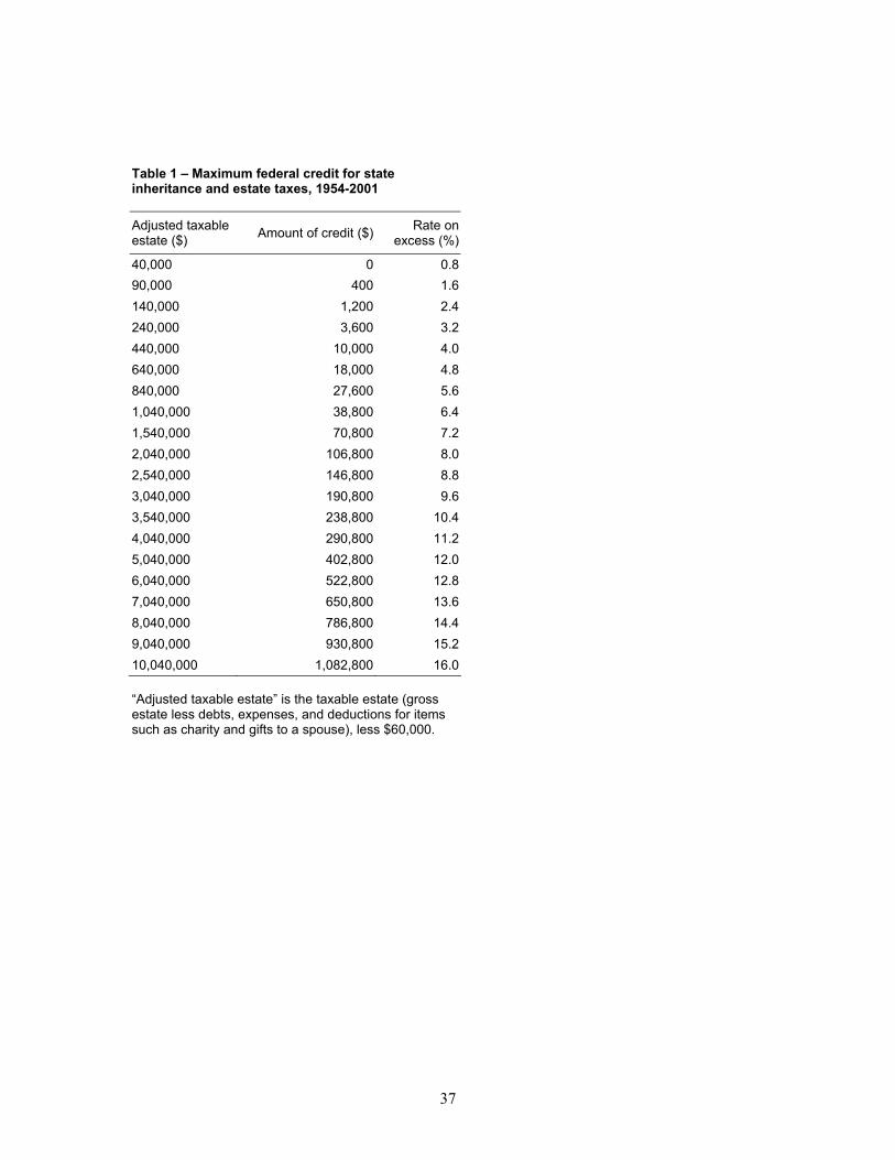
37

Table 1 – Maximum federal credit for state inheritance and estate taxes, 1954-2001

Adjusted taxable estate ($) Amount of credit ($) Rate on

excess (%)

40,000 0 0.890,000 400 1.6140,000 1,200 2.4240,000 3,600 3.2440,000 10,000 4.0640,000 18,000 4.8840,000 27,600 5.61,040,000 38,800 6.41,540,000 70,800 7.22,040,000 106,800 8.02,540,000 146,800 8.83,040,000 190,800 9.63,540,000 238,800 10.44,040,000 290,800 11.25,040,000 402,800 12.06,040,000 522,800 12.87,040,000 650,800 13.68,040,000 786,800 14.49,040,000 930,800 15.210,040,000 1,082,800 16.0 “Adjusted taxable estate” is the taxable estate (gross estate less debts, expenses, and deductions for items such as charity and gifts to a spouse), less $60,000.

38

State 1965 1970 1975 1980 1985 1990 1995 2000 State 1965 1970 1975 1980 1985 1990 1995 2000AK 1.1 MS 0.5 0.4 0.4AL MT 2.9 2.8 2.8 2.8AR NC 2.5 2.5 2.4 1.8 1.7AZ ND 4.1 4.0 2.0CA 2.6 4.3 4.6 5.1 NE 0.1CO 2.4 2.8 3.4 0.0 NHCT 2.8 2.6 2.3 2.2 2.6 2.6 2.8 NJ 0.8 0.8 0.8 1.9 1.8DC 0.5 0.3 0.9 0.8 1.0 NM 0.2DE 1.6 1.6 2.1 2.2 2.1 1.9 1.8 NVFL NY 2.3 2.2 2.0 1.9 1.9 2.0 2.0GA OH 1.5 2.5 2.5 2.6 2.7 2.6 2.5 2.4HI 2.0 1.8 1.7 1.3 OK 3.8 3.8 2.9 3.0 0.9 1.1 1.2IA 1.3 1.9 1.9 1.7 2.1 2.5 2.2 OR 2.8 2.7 2.9 8.3 0.7ID 2.7 2.6 2.7 2.0 PA 1.4 5.0 4.5 3.9 3.4 3.1 2.7 2.5IL 1.0 0.9 0.7 0.2 RI 4.1 4.3 4.4 4.4 2.9IN 1.6 1.4 1.0 0.8 0.7 0.6 0.5 SC 2.9 3.0 3.1 3.0 3.9 1.8KS 0.7 0.5 0.3 0.0 0.1 0.1 SD 1.7 2.9 3.0 3.7 3.5 3.3 3.1 3.2KY 2.6 2.5 2.4 2.4 3.0 3.3 0.9 TN 2.4 3.4 3.9 3.2 0.2 0.0 0.2LA 2.0 1.8 1.3 0.8 0.3 TX 0.7 0.6 0.5MA 2.5 3.2 3.1 6.6 6.7 7.1 6.5 UT 6.0 6.1 5.9MD 0.2 VA 0.5 0.3ME 1.1 0.9 0.6 2.5 0.1 VT 2.1 1.9 4.8MI 2.3 2.2 1.9 1.6 1.9 2.0 WA 1.8 2.3 2.9 3.6MN 2.8 2.7 2.6 1.0 0.2 WI 4.0 3.9 3.9 4.0 4.4 0.2MO 1.2 1.0 0.8 0.5 WV 2.5 2.2 1.8 1.7

WY 0.9 0.5U.S. mean 1.7 1.8 1.8 1.6 1.0 0.7 0.5 0.2Std. dev. 1.3 1.5 1.6 1.9 1.5 1.4 1.2 0.6Notes: blank indicates zero. Table depicts combined federal-state inhertance and estate tax liablity as a percentage of net worth, minus what it would be in a state that only operates a "soak-up" tax.

Table 2 -- Effective average state inheritance and estate tax rate (percent) on a $1 million (in constant 1996 dollars) bequest divided equally between two adult children (EIATR)

39

Table 3 -- Effective average state inheritance and estate tax rates on a bequest divided equally between two adult children, at different estate values

Estate value (constant 1996 $) 1965 1970 1975 1980 1985 1990 1995 2000 $575,000 1.7 1.9 1.8 1.6 1.7 1.4 1.1 0.4 $1,000,000 1.7 1.8 1.8 1.6 1.0 0.7 0.5 0.2 $1,625,000 1.6 1.7 1.7 1.5 0.9 0.6 0.5 0.1 $3,500,000 1.4 1.6 1.5 1.2 0.7 0.4 0.3 0.0 $10,000,000 0.9 1.0 0.8 0.6 0.3 0.2 0.2 0.0

Values shown are un-weighted means of state effective average tax rates on a bequest of the indicated value, as a percentage of net worth.

40

Table 4 – Variable definitions and descriptive statistics Variable Description Mean Min Max Std.

Dev

OBS Number of sampled estate tax returns in cell 64 0 1,374 114

RETURNS Estimated population of federal estate tax returns in cell (OBS times sampling weight) 257 0 5,760 503

EIATR Effective state average estate and inheritance tax rate at midpoint of wealth category 0.007 0 0.077 0.014

INCATR Effective state average income tax rate at similar point of elderly income distribution 0.021 0 0.057 0.014

SALESTX Statutory state retail sales tax rate, adjusted for any savings from federal income tax deductibility 0.034 0 0.080 0.021

PROPTX State and local property tax revenues as a share of state personal income, adjusted for any savings from federal income tax deductibility

0.020 0.003 0.054 0.008

GOVEXRAT State and local government expenditures as a share of state personal income 0.181 0.107 0.502 0.043

POP State population, thousands 4,764 271 32,683 5,231

T5YSHR Share of individuals / couples aged 25-59 in the state who fall into the top 5% of the national income distribution for that age group

0.043 0.018 0.153 0.017

DTHRAT State deaths, aged 45 and above (excluding fed. estate tax return deaths) divided by state population 0.007 0.002 0.011 0.001

UNEMP State unemployment rate 0.059 0.022 0.155 0.021

NCMPRE82 Dummy variable for “not a community property state” interacted with dummy for years before 1982 0.171 0 1 0.377

CRIME State crime rate (crimes per 100 population) 4.602 0.502 12.174 1.826

STKSHR Share of assets held in stocks in 1976 for each state-wealth combination 0.373 0.044 0.789 0.156

SP500 S & P 500 stock price index 373 88 1,085 269

HOUSEPR State-specific housing price index (expressed in thousands of dollars) 73 11 320 41

PCPI State per capita personal income (in thousands of 1996 dollars) 20.906 3.197 35.939 4.753

SUN Fraction of days that are clear or partly cloudy 0.494 0.300 0.690 0.076

HEATING Heating degree days / 1000 5.066 0 8.968 2.175

COOLING Cooling degree days / 1000 1.226 0 4.474 0.955

Years included: 1965, 1969, 1976, 1982, 1985-1998 Number of state-wealth-year cells: 3,713 Number of underlying sampled returns: 236,829 Estimated population of returns represented: 955,987 Mean values presented above are un-weighted means across all 3,713 cells.

41

No state-wealth dumies or state

time trends

Including dummies for each state - wealth class combination

Including state-wealth dummies

and state-specific time

trends(1) (2) (3)

EIATR -0.639 -1.870 -1.382(0.173)** (0.249)** (0.309)**

INCATR -2.378 -2.733 -1.491(0.239)** (0.456)** (0.689)*

SALESTX -0.368 -3.339 -2.791(0.236) (0.419)** (0.625)**

PROPTX 14.379 -0.404 -3.389(0.513)** (1.057) (1.383)*

GOVEXRAT 0.371 0.396 0.061(0.123)** (0.289) (0.346)

LN(POP) 1.010 1.034 1.456(0.003)** (0.030)** (0.164)**

LN(T5YSHR) 0.322 0.374 0.263(0.015)** (0.032)** (0.054)**

LN(DTHRAT) 1.194 0.016 -0.763(0.020)** (0.066) (0.119)**

UNEMP -3.585 -2.344 -2.057(0.197)** (0.251)** (0.275)**

NCMPRE82 0.247 0.127 0.154(0.011)** (0.017)** (0.029)**

CRIME 0.062 0.075 0.033(0.003)** (0.005)** (0.006)**

STKSHR*LN(SP500) -0.091 -0.004 0.356(0.005)** (0.034) (0.046)**

LN(HOUSEPR) 0.660 0.244 0.398(0.015)** (0.023)** (0.036)**

SUN 0.443(0.038)**

HEATING -0.036(0.002)**

COOLING -0.004(0.005)

State / wealth dummies? No Yes YesState-specific time trends? No No Yes

Standard errors are in parentheses.* significant at 5%; ** significant at 1%

Each coefficient represents the effect of a characteristic of state j and wealth class k on ln[Pjkt(1-Pjkt)], where Pjkt is the proportion of national returns in wealth class k that are located in state j.

Table 5 -- Conditional logit estimates of how state characteristics affect the reported locations of federal estate tax return filers

42

Omit LN(T5YSHR)

Omit LN (DEATHRAT)

Omit STKSHR* LN(SP500)

Omit LN (HOUSEPR)

(1) (2) (3) (4)

EIATR -1.735 -1.871 -1.869 -2.012(0.249)** (0.249)** (0.249)** (0.249)**

INCATR -2.246 -2.718 -2.729 -1.801(0.454)** (0.452)** (0.455)** (0.448)**

SALESTX -3.069 -3.349 -3.336 -3.474(0.417)** (0.416)** (0.418)** (0.418)**

PROPTX 2.353 -0.398 -0.411 -1.683(1.031)* (1.057) (1.056) (1.051)

GOVEXRAT -0.552 0.392 0.391 0.743(0.279)* (0.289) (0.287) (0.286)**

Add LN(PCPI) Omit PROPTXOmit

GOVEXRAT(5) (6) (7)

EIATR -2.208 -1.884 -1.863(0.250)** (0.247)** (0.249)**

INCATR -0.780 -2.693 -2.650(0.465) (0.444)** (0.452)**

SALESTX -2.376 -3.336 -3.213(0.420)** (0.418)** (0.408)**

PROPTX -3.316 0.193(1.060)** (0.962)

GOVEXRAT 0.873 0.350(0.288)** (0.263)

Standard errors are in parentheses.* significant at 5%; ** significant at 1%

Table 6 -- Sensitivity of fiscal variable coefficients to omission or addition of variables (conditional logit with state-wealth dummies)

Each coefficient represents the effect of a characteristic of state j and wealth class k on ln[Pjkt(1-Pjkt)], where Pjkt is the proportion of national returns in wealth class k that are located in state j in year t.

43

Weighted least squares

Weighted 2SLS, using 5-year lag

tax rates as instruments

(1) (2) (3)

EIATR -1.996 -2.667 -2.161(0.739)** (1.276)* (0.467)**

INCATR -1.651 -3.824 -0.406(1.211) (2.334) (1.279)

SALESTX -2.985 -3.348 -4.049(0.936)** (2.026) (1.079)**

PROPTX -3.941 -6.626 -4.949(2.975) (4.750) (2.859)

GOVEXRAT 0.689 0.300 -0.321(0.798) (0.484) (0.721)

LN(POP) 1.355 1.270 1.518(0.085)** (0.089)** (0.515)**

LN(T5YSHR) 0.387 0.402 0.297(0.083)** (0.086)** (0.109)**

LN(DTHRAT) 0.243 0.300 -0.419(0.228) (0.237) (0.366)

UNEMP -1.272 -0.871 -1.176(0.565)* (0.652) (0.474)*

NCMPRE82 0.030 0.030 0.093(0.020) (0.019) (0.023)**

CRIME 0.036 0.039 0.023(0.011)** (0.011)** (0.010)*

STKSHR*LN(SP500) 0.097 0.098 0.314(0.095) (0.094) (0.108)**

LN(HOUSEPR) 0.219 0.224 0.348(0.064)** (0.071)** (0.076)**

State / wealth dummies? Yes Yes YesState-specific time trends? No No Yes

Robust standard errors, with clustering by state, are in parentheses.* significant at 5%; ** significant at 1%

Dependent variable is ln[Pjkt(1-Pjkt)], where Pjkt is the proportion of nationwide returns in a wealth class k located in state j in year t.

Weighted least squares,

including state-wealth dummies

and state-specific time

trends

Including dummies for each state -wealth class combination

Table 7 -- Linear regression estimates of how state characteristics affect the log-odds of a federal estate tax return being filed in a state

44

Dependent variable: EIATR at time t

Lagged EIATR 0.444704(0.039012)**

Lagged LN[Pjk/(1-Pjk)] -0.000010(0.000203)

INCATR 0.060229(0.086142)

SALESTX 0.018557(0.082846)

PROPTX 0.027537(0.189695)

GOVEXRAT 0.030808(0.023357)

LN(POP) 0.004540(0.004373)

LN(T5YSHR) 0.003142(0.003913)

LN(DTHRAT) 0.015957(0.008999)

UNEMP 0.073942(0.039200)

NCMPRE82 0.000139(0.001442)

CRIME 0.000235(0.000720)

STKSHR*LN(SP500) -0.006732(0.002976)*

LN(HOUSEPR) -0.003705(0.003881)

State / wealth dummies? YesState-specific time trends? No

* significant at 5%; ** significant at 1%

Table 8 -- Granger causality test for effect of lagged estate tax returns on current state estate and inheritance tax rate

"Lagged" values are from 5 years before, or the year closest to 5 years before in cases where there are gaps in the data.Robust standard errors, with clustering by state, are in parentheses.

45

Top wealth classOther wealth

classes(1) (2)

EIATR -3.952 -1.843(1.700)* (0.696)*

INCATR -4.272 -1.129(2.006)* (1.390)

SALESTX -1.846 -3.190(2.227) (0.950)**

PROPTX -0.568 -3.540(7.804) (2.991)

GOVEXRAT 0.355 0.687(1.372) (0.830)

LN(POP) 1.339 1.358(0.186)** (0.077)**

LN(T5YSHR) 0.369 0.379(0.114)** (0.087)**

LN(DTHRAT) 0.402 0.217(0.371) (0.233)

UNEMP -2.881 -1.073(1.203)* (0.529)*

NCMPRE82 0.035 0.029(0.034) (0.019)

CRIME 0.069 0.029(0.016)** (0.012)*

STKSHR*LN(SP500) 0.100 0.098(0.136) (0.104)

LN(HOUSEPR) 0.036 0.249(0.091) (0.067)**

State / wealth dummies? Yes YesState-specific time trends? No No

* significant at 5%; ** significant at 1%

Dependent variable is ln[Pjkt(1-Pjkt)], where Pjkt is the proportion of nationwide returns in a wealth class k located in state j in year t. Estimated by weighted least squares.

Table 9 -- Linear regression estimates of how state characteristics affect the log-odds of a federal estate tax return being filed in a state: split sample by wealth class

Robust standard errors, with clustering by state, are in parentheses.

46

Size of gross estate, 2001 dollars

Average state tax rate at

mean taxable estate in class

$625,000 - $1,000,000 3.9$1,000,000 - $2,500,000 5.1$2,500,000 - $5,000,000 3.7$5,000,000 - $10,000,000 4.6$10,000,000 - $20,000,000 5.0$20,000,000 or more 4.6All returns 4.5

Table 10 -- Value of EIATR in 2006 for a state that decouples from federal law

Assumes the state estate tax is frozen based on parameters of federal law effective in 2001.

Estimated coefficient (β) on EIATR

Percentage of revenue lost

Table 5, column (3), β = -1.38 6.2β = 2 8.9Table 7, column (2), β = -2.67 11.9Table 9, β's = -3.95, -1.84 13.5

Table 11 -- Estimated percentage of decoupled state estate tax revenue lost to induced changes in reported residence

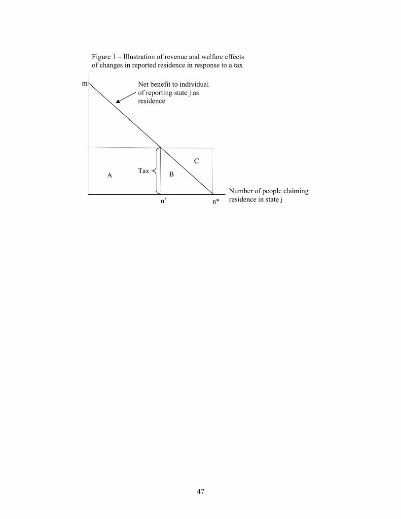
47

Number of people claiming residence in state j

Net benefit to individual of reporting state j as residence

Figure 1 – Illustration of revenue and welfare effects of changes in reported residence in response to a tax

Tax B A

C

n* n’

m

48

State 1965 1975 1985 1995 State 1965 1975 1985 1995AK 1.9 2.2 MS 1.0 1.1 1.7 2.4AL 1.5 1.3 1.4 1.8 MT 1.7 2.0 1.8 3.1AR 1.4 2.0 2.4 3.4 NC 2.7 2.6 2.9 4.0AZ 1.0 1.7 1.6 2.2 ND 1.7 1.8 1.3 2.3CA 1.4 2.9 3.3 4.2 NE 1.3 2.5 3.5CO 1.9 1.8 1.1 2.1 NH 0.8 0.7 0.9 1.1CT 0.7 2.6 2.8 NJ 1.0 1.2 2.5DC 1.1 2.4 3.6 5.0 NM 0.6 1.7 1.9 3.7DE 1.8 0.5 1.8 3.7 NVFL NY 2.4 3.3 3.8 3.8GA 1.7 2.0 2.1 2.6 OH 0.9 2.2 3.0HI 2.1 2.7 3.2 4.5 OK 1.2 1.1 2.0 3.4IA 1.1 1.6 2.0 2.9 OR 2.8 2.5 2.4 3.5ID 2.4 2.6 2.8 4.5 PA 0.9 1.1 1.7IL 1.1 1.1 1.7 RI 1.8 3.0 4.4IN 0.9 0.9 1.3 2.1 SC 1.4 1.5 1.5 3.2KS 1.5 1.3 1.6 3.7 SDKY 1.4 1.4 1.3 0.2 TN 1.3 1.2 1.4 1.7LA 0.7 0.7 0.7 1.5 TXMA 2.7 4.1 3.7 5.3 UT 2.1 1.3 1.5 2.8MD 1.7 1.8 1.9 2.8 VA 1.9 1.8 2.1 2.7ME 1.2 3.1 4.3 VT 2.3 2.8 3.4 4.0MI 1.6 2.1 2.5 WAMN 2.5 3.2 3.0 4.4 WI 2.9 3.5 3.3MO 0.9 1.2 1.2 2.1 WV 0.8 1.4 2.8 3.2

WYU.S. mean 1.2 1.5 1.8 2.5Std. dev. 0.9 1.0 1.1 1.5Notes: blank indicates zero. See text for description of INCATR.

Table A.1 -- Value of INCATR for $750,000 - $1.25 million wealth class, selected years (expressed as percentage)

49

State 1965 1975 1985 1995 State 1965 1975 1985 1995AK MS 2.5 3.2 3.5 7.0AL 2.8 2.6 2.3 4.0 MTAR 2.1 1.9 2.3 4.5 NC 2.1 1.9 1.7 4.0AZ 2.1 2.6 2.9 5.0 ND 1.6 2.6 2.3 5.0CA 2.1 3.1 2.8 6.0 NE 1.6 2.0 5.0CO 1.4 1.9 1.7 3.0 NHCT 2.5 3.9 4.4 6.0 NJ 3.2 3.5 6.0DC 2.1 3.2 3.5 6.0 NM 2.1 2.6 2.2 5.0DE NV 1.4 1.9 3.4 6.5FL 2.1 2.6 2.9 6.0 NY 0.0 2.6 2.3 4.0GA 2.1 1.9 1.7 4.0 OH 2.1 2.6 2.9 5.0HI 2.4 2.6 2.3 4.0 OK 1.4 1.3 1.9 4.5IA 1.4 1.9 2.3 5.0 ORID 1.9 2.3 5.0 PA 3.5 3.9 3.5 6.0IL 2.5 2.6 2.9 6.3 RI 2.5 3.2 3.5 7.0IN 1.4 2.6 2.9 5.0 SC 2.1 2.6 2.9 5.0KS 1.8 1.9 1.7 4.9 SD 1.4 2.6 2.3 4.0KY 2.1 3.2 2.9 6.0 TN 2.1 2.3 3.2 6.0LA 1.4 1.9 2.3 4.0 TX 1.4 2.6 2.4 6.3MA 1.9 2.9 5.0 UT 2.1 2.6 2.7 5.0MD 2.1 2.6 2.9 5.0 VA 1.9 1.7 3.5ME 2.8 3.2 2.9 6.0 VT 1.9 2.3 5.0MI 2.8 2.6 2.3 4.0 WA 2.1 1.9 2.9 6.5MN 2.6 3.5 6.5 WI 2.1 2.6 2.9 5.0MO 2.1 1.9 2.4 4.2 WV 2.8 2.9 3.8 6.0

WY 1.4 1.9 1.8 4.0U.S. mean 1.5 2.2 2.4 4.6Std. dev. 1.0 0.9 1.0 1.8Notes: blank indicates zero. See text for description of SALESTX.

Table A.2 -- Value of SALESTX for $750,000 - $1.25 million wealth class, selected years (expressed as percentage)

50

State 1965 1975 1985 1995 State 1965 1975 1985 1995AK 1.0 1.0 2.9 3.0 MS 1.8 1.3 1.2 1.7AL 0.9 0.6 0.6 0.8 MT 4.0 2.8 2.9 3.2AR 1.6 1.0 0.9 1.0 NC 1.5 1.3 1.1 1.5AZ 3.5 2.2 1.5 2.2 ND 3.2 1.6 1.5 2.2CA 3.5 2.8 1.4 2.0 NE 3.8 2.5 2.2 2.8CO 3.4 1.8 1.8 2.0 NH 3.4 3.0 2.4 4.0CT 2.7 2.7 2.0 3.0 NJ 3.3 3.2 2.3 3.6DC 1.8 1.4 2.2 2.8 NM 1.6 1.0 0.7 1.0DE 1.1 1.0 0.7 1.1 NV 2.5 1.9 1.1 1.4FL 2.2 1.5 1.4 2.3 NY 3.1 2.9 2.3 3.1GA 1.7 1.7 1.2 1.9 OH 2.6 1.8 1.4 2.1HI 1.3 1.1 1.1 1.4 OK 1.9 1.1 0.9 1.2IA 3.6 2.3 2.2 2.8 OR 2.9 2.4 2.5 2.4ID 3.1 1.5 1.3 1.9 PA 1.9 1.4 1.4 2.1IL 2.6 2.2 1.9 2.7 RI 2.7 2.4 2.2 3.3IN 2.9 2.1 1.6 2.3 SC 1.3 1.1 1.2 2.0KS 3.8 2.2 1.9 2.3 SD 4.0 2.6 2.2 2.7KY 1.5 1.0 0.9 1.2 TN 1.8 1.3 1.0 1.3LA 1.5 0.9 0.8 1.1 TX 2.5 1.7 1.8 2.4MA 3.6 3.7 1.9 2.6 UT 2.9 1.6 1.6 1.9MD 2.2 1.6 1.3 1.9 VA 1.7 1.4 1.3 2.0ME 3.2 2.4 2.1 3.5 VT 3.1 3.1 2.3 3.6MI 2.7 2.6 2.3 1.9 WA 2.0 1.8 1.5 2.3MN 3.7 2.0 1.8 2.6 WI 3.3 2.4 2.3 3.2MO 2.2 1.7 0.9 1.7 WV 1.6 1.1 1.0 1.4

WY 3.8 2.3 4.4 3.0U.S. mean 2.5 1.9 1.7 2.2Std. dev. 0.9 0.7 0.7 0.8Notes: blank indicates zero. See text for description of PROPTX.

Table A.3 -- Value of PROPTX for $750,000 - $1.25 million wealth class, selected years (expressed as percentage)

51

References

Anderson, J.A. (1972). “Separate sample logistic discrimination.” Biometrika Vol. 59, No. 1 (March): pp. 19-35. Bakija, Jon. 2004a. “Documentation for a Federal-State Inheritance and Estate Tax Calculator Covering the Years 1900-2002.” Working paper, Williams College. Bakija, Jon. 2004b. “Documentation for a Federal-State Personal Income Tax Calculator Covering the Years 1900-2002.” Working paper, Williams College. Baldwin, Richard E., and Paul Krugman. 2004. "Agglomeration, Integration, and Tax Harmonization." European Economic Review. Vol. 48, No. 1, (February): pp. 1-23. Bennefield, Robert L. 2003. Home Values 2000: A Census 2000 Brief. Washington: U.S. Bureau of the Census. <www.census.gov/prod/2003pubs/c2kbr-20.pdf>. Bertrand, Marianne, Esther Duflo, and Sendil Mullainathan. 2004. “How Much Should We Trust Difference-In-Differences Estimates?” Quarterly Journal of Economics. Vol. Vol. 119, No. 1 (February): pp. 249-275. Blank, Rebecca M. 1988. “The Effect of Welfare and Wage Levels on the Location Decisions of Female-Headed Households.” Journal of Urban Economics. Vol. 24, pp. 186-211. Blumkin, Tomer, and Efraim Sadka. 2004. “Taxation with Intended and Accidental Bequests.” Journal of Public Economics, Vol. 88, Nos. 1-2 (January), pp. 1-21. Conway, Karen Smith and Andrew J. Houtenville. 2001. "Elderly Migration and State Fiscal Policy: Evidence from the 1990 Census Migration Flows." National Tax Journal. Vol. 54, No. 1, pp. 103-123. Conway, Karen Smith and Jonathan C. Rork. 2004a. "Diagnosis Murder -- The Death of State ‘Death’ Taxes." Forthcoming, Economic Inquiry. Conway, Karen Smith and Jonathan C. Rork. 2004b. " State ‘Death’ Taxes and Elderly Migration – The Chicken or the Egg?" Working Paper, University of New Hampshire. Cosslett, S. 1981. Efficient Estimation of Discrete-Choice Models. In Charles Manski, and Daniel McFadden, eds., Structural Analysis of Discrete Data with Econometric Applications, Cambridge, Mass.: MIT Press, 51-111. Davies, Paul S., Michael J. Greenwood, and Haizheng Li. 2001. “A Conditional Logit Approach to U.S. State-to-State Migration.” Journal of Regional Science, Vol. 41, No. 2, pp. 337-360.

52

Duncombe, W., M. Robbins, and D. Wolf. 2003. “Place Characteristics and Residential Location Decisions Among the Retirement-Age Population.” Journal of Gerontology: Social Sciences. Vol. 58B: S244-S252. Farnham, Martin, and Purvi Sevak. 2004. “Tiebout Non-Sorting? Empty-Nest Migration and the Local Fiscal Bundle.” working paper, Population Studies Center, University of Michigan (Report No. 04-558, May). Feenberg, Daniel Richard, and Elizabeth Coutts. 1993. "An Introduction to the TAXSIM Model," Journal of Policy Analysis and Management, Vol. 12, No. 1, (Winter), pp. 189-194. Feldstein, Martin, and Marian Vaillant Wrobel. 1998. "Can State Taxes Redistribute Income?" Journal of Public Economics. Vol. 68, No. 3 (June): pp. 469-396. Forfield Inc. 2003. “Status of State Death Taxes: Summary.” July. <http://www.forefield.com/stateestate/> (accessed June 17, 2004). Gramlich, Edward M., and Deborah S. Laren. 1984. “Migration and Income Redistribution Responsibilities.” Journal of Human Resources. Vol. 19, No. 4 (Autumn), pp. 489-511. Greene, William H. 2000. Econometric Analysis, 4th Edition. Upper Saddle River, NJ: Prentice-Hall, Inc. Greene, William H. 2002. Limdep Version 8.0 Econometric Modeling Guide. Plainview, NY: Econometric Software, Inc. Gresenz, Carole Roan. 1997. “An Empirical Investigation of the Role of AFDC Benefits in Location Choice.” Rand Labor and Population Program Working Paper Series, No. 97-05 (April). Johnson, Barry W. 1994. "Estate Tax Returns, 1989-1991." In Barry W. Johnson, ed., Compendium of Federal Estate Tax and Personal Wealth Studies. Washington: IRS Statistics of Income Division. Johnson, Barry W., Jakob M. Mikow, and Martha Britton Eller. 2001. "Elements of Federal Estate Taxation." In William Gale, James R. Hines Jr., and Joel Slemrod, eds., Rethinking Estate and Gift Taxation. Washington: Brookings Institution Press. Joulfaian, David and Kathleen McGarry. 2004. “Estate and Gift Tax Incentives and Inter Vivos Giving.” National Tax Journal, Vol. 57, No. 2, Part 2 (June): pp. 429-444. Kaestner, Robert, Neeraj Kaushal, and Gregg Van Ryzin. 2003. “Migration Consequences of Welfare Reform.” Journal of Urban Economics. Vol. 53, No. 3 (May): pp. 357-376.

53

Kiefer, Donald, Robert Carroll, Janet Holtzblatt, Allen Lerman, Janet McCubbin, David Richardson, and Jerry Tempalski. 2002. “The Economic Growth and Tax Relief Reconciliation Act of 2001: Overview and Assessment of Effects on Taxpayers.” National Tax Journal 55, No. 1 (March): pp. 89-117. Kopczuk, Wojciech, and Joel Slemrod. 2001. “The Impact of the Estate Tax on Wealth Accumulation and Avoidance Behavior.” in William G. Gale, James R. Hines, and Joel Slemrod, eds., Rethinking Estate and Gift Taxation. Washington: Brookings Institution Press. Levine, Phillip B., and David J. Zimmerman. 1999. “An Empirical Analysis of the Welfare Magnet Debate Using the NLSY.” Journal of Population Economics. Vol. 12, No. 3 (August): pp. 391-409. Moretti, Enrico. 2003. “Human Capital Externalities in Cities.” NBER Working Paper No. 9641 (April). McFadden, Daniel. 1974. Conditional Logit Analysis of Qualitative Choice Behavior.” In P. Zarembka, ed., Frontiers in Econometrics, New York: Academic Press, pp. 105-142. McNichol, Elizabeth. 2004. “Many States are Decoupling from the Federal Estate Tax Cut.” Center for Budget and Policy Priorities. (Jan. 14)

<http://www.centeronbudget.org/5-23-02sfp.htm>. McNichol, Elizabeth, Iris J. Lav and Joseph Llobrera. 2003. “States Can Retain Their Estate Taxes Even as the Federal Estate Tax is Phased Out.” Center for Budget and Policy Priorities, (Feb. 4) <http://www.cbpp.org/1-31-02sfp.htm>. Mirrlees, J.A. 1982. “Migration and Optimal Income Taxes.” Journal of Public Economics. Vol. 18, No. 3 (August): pp. 319-341 . Moffitt, Robert. 2002. “Documentation for Moffitt Welfare Benefits File.” Mimeo, Johns Hopkins University <http://www.econ.jhu.edu/People/Moffitt/DataSets.html>. Moulton, Brent R. 1990. “An Illustration of a Pitfall in Estimating the Effects of Aggregate Variables in Micro Units,” Review of Economics and Statistics, Vol. 72, No. 2 (May): pp. 334–338. Musgrave, Richard. 1959. The Theory of Public Finance. New York: McGraw-Hill. Nechyba, Thomas J. and Robert P. Strauss. 1998. “Community Choice and Local Public Services: A Discrete Choice Approach.” Regional Science and Urban-Economics. Vol. 28, No. 1, pp. 51-73. Oates, Wallace E. 1972. Fiscal Federalism. New York: Harcourt Brace Jovanovich.

54

Office of Federal Housing Enterprise Oversight (OFHEO). 2004. Housing Price Index. <http://www.ofheo.gov/download.asp>. Page, Benjamin R. 2003. “Bequest Taxes, Inter Vivos Gifts, and the Bequest Motive.” Journal of Public Economics. Vol. 87, No. 5-6 (May): pp. 1219-1229. Pauly, Mark V. 1973. “Income Redistribution as a Local Public Good.” Journal of Public Economics. Vol. 2, No. 1 (February): pp. 35-58. Persson, Torsten, and Guido Tabellini. 1999. “Political Economics and Public Finance.” National Bureau of Economic Research Working Paper No. 7097. (April). Prentice, R.L. and Pyke, R. (1979). Logistic Disease Incidence Models and Case-control Studies, Biometrika Vol. 66, No. 3 (September): pp. 403-411. Ruggles, Steven, Matthew Sobek et al. 2003. “Integrated Public Use Microdata Series: Version 3.0” Minneapolis: Historical Census Projects, University of Minnesota. <http://www.ipums.umn.edu/usa/> Schoenblum, Jeffrey A. 1982. Multistate and Multinational Estate Planning. Boston: Little, Brown and Co. Slemrod, Joel. 1998. “Methodological Issues in Measuring and Interpreting Taxable Income Elasticities.” National Tax Journal. Vol. 51, No. 4 (December): pp. 773-788. U.S. Bureau of the Census. Various Years. Statistical Abstract of the United States. Washington: GPO. U.S. Bureau of the Census. Various Years. State Government Finances. <http://www.census.gov/govs/www/state.html>. U.S. Bureau of Economic Analysis. 2004. National Income and Product Accounts of the United States. <http://www.bea.gov/>. U.S. Centers for Disease Control. CDC Wonder Web Page <http://wonder.cdc.gov>. U.S. Department of Housing and Urban Development. 2004. U.S. Housing Market Conditions. 1st Quarter (May). <http://www.huduser.org/periodicals/ushmc.html> U.S. Federal Bureau of Investigation. Various Years. Uniform Crime Reports for the United States. Washington: GPO. U.S. National Center for Health Care Statistics. Various Years. Vital Statistics of the U.S. Washington: GPO.

55

U.S. Office of Management and Budget. 2004. Budget of the United States Government, Fiscal Year 2005. Washington: GPO.

56

Endnotes 1 An earlier version of this paper was titled “The Impact of Progressive State Taxes on the Locations and Estates of the Rich.” We would like to thank Barry Johnson for providing us with the tabulations of federal estate tax return data, and Wojciech Kopczuk for help with the data and for many invaluable suggestions. Karen Conway, Martin Farnham, Jim Poterba, Jonathan Rork, and seminar participants at Brookings, the Harvard/MIT joint public economics seminar, University of Michigan, University of Virginia, Wesleyan, William and Mary, and Williams also provided helpful comments for which we are grateful. Finally, we would like to thank Vladimir Andonov, Manijeh Azmoodeh, Sebastien Bradley, Diana Carligeanu, Misha Dworsky, Alex Fischer, Brennan Kelly, Edvard Major, Chris Lyddy, Rochan Raichura, Hui Shan, and Drew Thomas for outstanding research assistance that was essential to constructing the tax calculators used in this paper. 2 Pauly (1972) discusses the implications of redistribution as a local public good. 3 Mirrlees (1982) presents a model where the government of a jurisdiction chooses a non-linear income tax schedule to maximize the aggregate utility of its residents, income has diminishing marginal social utility (creating a motive for redistributive taxation), and people can emigrate. He finds that the optimal degree of redistributive taxation is inversely related to the elasticity of the number of residents with respect to changes in their after-tax incomes. In this particular model Mirrlees abstracts from labor supply decisions by treating pre-tax income as fixed, which is appropriate to our application, as our evidence mainly pertains to the retirement-age segment of the population. In a model where redistribution is a local public good and high-income people are heterogeneous in their willingness to move, Pauly (1972) also finds that the optimal degree of redistributive taxation in a jurisdiction is a declining function of the degree of mobility in response to taxes. He further notes that in this context, “a reduction in the total taxes of those most likely to move, in order to induce them to stay, is a way of attaining optimality...,” a point that should carry over to other sorts of models of optimal state tax policy as well (Pauly 1972, p. 50). This would suggest that if the location decisions of wealthy elderly people are particularly flexible and responsive to taxation compared to others with high incomes, it might not make sense for a state to tax them at a higher rate than others through estate and inheritance taxation, ceteris paribus. 4 See, for example, Gramlich and Laren (1984), Blank (1988), Gresenz (1997), Levine and Zimmerman (1999), and Kaestner, Kaushal, and Van Ryzin (2003). 5 One piece of indirect evidence comes from Feldstein and Wrobel (1998), who find, using cross-sectional data from the Census Current Population Survey, that states which operate more progressive tax systems also have more unequal wage distributions. This would be consistent with out-migration of high-skill labor and in-migration of low-skill labor in response to progressive taxes, although it would also be consistent with a number of other possible explanations, such as reverse causality due to political economy considerations. 6 See Kiefer, et al (2002) for a summary of the provisions of the 2001 tax act affecting federal and state estate and inheritance taxes. 7 See the discussion of Table 10 below for the basis of this estimate. Estates below $675,000 would be exempt in this example, as that was the federal estate tax exemption that applied in 2001, and state soak-up taxes did not begin to apply until the point where federal estate tax liability began to accrue. 8 McNichol (2004) discusses the status of state estate taxes. As of January 14, 2004, jurisdictions where the former soak-up estate tax is scheduled to persist after the federal credit is eliminated include the District of Columbia, Kansas, Illinois, Maine, Maryland, Massachusetts, Minnesota, Nebraska, New Jersey, New York, North Carolina, Ohio, Oregon, Rhode Island, Vermont, Virginia, Washington, and Wisconsin.

57

9 Conway and Houtenville (2001) and Conway and Rork (2004), for example, both use revenue-based measures, although they also try some alternatives – for instance, the EI tax on a $60,000 estate in the first case, and dummy variables for whether the state imposed its own EI tax, as opposed to relying exclusively on a soak-up tax, in the latter case. 10 As noted above, Conway and Houtenville (2001) tried this approach. Duncombe, Robbins, and Wolf (2003) constructed a state estate tax average rate and a state inheritance tax average rate, each calculated on an $822,000 bequest to a spouse using 1987 law, and applied it to all individuals in their sample. 11 Census PUMS micro-data, which in recent waves includes 5 percent samples of the U.S. population, also undoubtedly includes many wealthy people, but does not contain information on wealth, and top-codes income. It does provide information on state of residence in the current year and 5 years before, allowing analysis of migration decisions, but it will miss many moves by people who migrate within 5 years of dying. Nonetheless, the PUMS data sets offer a promising avenue for further migration research. 12 Slemrod (1998) provides a review of this literature. 13 See Johnson, Mikow, and Eller (1998) for an overview of historical provisions of the federal estate tax through 1998, and Kiefer et al (2002) for a summary of changes since then. 14 See Johnson (1994), for example, for a discussion of the sample design. Note that returns in the highest gross estate size class were sampled at a 100% rate. 15 Our measure of net worth also adds back in any “special use valuation” discount that had been subtracted in the calculation of the gross estate. Such discounts were allowed starting in 1977 for farm and closely-held business property that met certain restrictions. This is a minor adjustment; for example, it only applied to about one percent of taxable estates filing between 1995 and 1998 (Johnson, Mikow, and Eller, 1998, p. 95). 16 A federal estate tax return was required of any decedent whose “gross estate” exceeded the exemption for the federal estate tax . 17 Note that since we are dealing with data spanning multiple years, each variable in this section should also have a subscript t representing the year of death. In this section we abstract from the time dimension and drop the time subscript to avoid cumbersome notation. 18 A number of studies have used the conditional logit approach to model migration or location decisions. The only ones to consider taxes are Duncombe, Robbins, and Wolf (2003), discussed above, and Nechyba and Strauss (1998), who estimate the effect of property taxes on community choice in New Jersey. Davies, Greenwood, and Li (2001) use a conditional logit to model individual migration choices among the states, but do not consider taxes. Gresenz (1997) uses the conditional logit to investigate the impact of welfare benefits on individual migration choices among the states. 19 We implement this in Stata via the following method. The data consists of 50 (prior to 1976, when DC is unavailable) or 51 (after 1976) rows, each containing the applicable characteristics of one state and an indicator variable for whether the state was actually chosen by the observations in the cell, for each of the 3,713 cells, for a total of 189,363 rows. We then estimate the conditional logit on this data with frequency weights applied to each cell, where the frequency weight is the number of sampled returns in the cell. This method is suggested by Greene (2002, section E19.4), who labels it a “conditional logit for frequency data.” 20 The fact that each observation in our conditional logit estimation was drawn through a stratified sampling technique is not a problem for our analysis, because the sampling rates do not vary systematically across states. In a logit framework, the standard approach to stratified samples is to control for dummy variables for each of the individual characteristics upon which the sample is stratified. This produces consistent

58

estimates of the parameters on the other variables -- see Anderson (1972), Prentice and Pyke (1979), and Cosslett (1981). In the conditional logit framework, these dummy variables difference out of the likelihood function because they are constant across the choices. The stratification in the estate tax return sample is based on year of death and two individual characteristics: gross estate class, and age at death. These all difference out of the conditional logit likelihood function, and are not systematically related to state of residence, so no special procedure is required regarding the sampling in order to obtain consistent estimates. 21 We discuss how we construct the representative characteristics of the “rest of the nation” further below. 22 As Greene suggests, the heteroskedasticity is corrected by weighting each observation by nkt jktP̂ (1-

jktP̂ ), where nkt is the number of sampled returns drawn in wealth class k in year t, and jktP̂ is the predicted

probability of someone in wealth class k and year t choosing state j. jktP̂ equals

[ ] [ ])('ˆ)('ˆ,~,~ 1/ ktjjktktjjkt XXXX ee −− + ββ

. As indicated in Greene, we compute initial consistent estimates of β

with an unweighted estimation of equation (7), use those initial consistent estimates to construct jktP̂ , and then iterate until the parameter estimates converge. This approach is necessary because the information provided by some cells is much noisier than for other cells. Intuitively, the nkt part of the weight puts a small weight on years and wealth classes where the number of sampled returns was small, and thus likely to suffer from larger sampling error. The jktP̂ (1- jktP̂ ) part of the weight puts a low weight on small states, which will also suffer from larger sampling error. Note that sampling error arises both because our data represents a random sample of the true population of estate tax returns, and because death produces a random sample of the metric we are really interested in, the number of wealthy elderly people living in a particular state at time t. This weighting procedure deals appropriately with variation across cells in both sorts of sampling error. The weighted estimate of population returns in each cell is used to construct the dependent variable (the log-odds ratio) in the linear regressions. We also tried using the unweighted number of observations in each cell to construct the log-odds ratio, and found very similar results, which should be expected given that the sampling rate does not vary systematically across states. Finally, a small problem in defining the dependent variable is posed by the fact that for 1.1 percent of the cells, Pjkt=0, and we can’t take the log of zero. We address this by adding 1 to the number of returns in each state. Note that cells with zero observations pose no special problems in the conditional logit framework. 23 Our discussions in this section and the next one draw on a very extensive study of historical federal and state tax laws, using sources such as federal tax returns and instructions dating back to 1917, historical state tax laws published in each state’s Annotated Statutes and Session Laws, and a variety of secondary sources published by organizations such as the Advisory Commission on Intergovernmental Relations, Commerce Clearing House, and Prentice-Hall. Bakija (2004a and 2004b) provides a complete discussion and reference list. 24 The fact that the maximum allowable federal credit for state EI taxes was the minimum of the amount calculated in Table 1 and federal tax liability (before applying the credit for state taxes) mattered in the following cases. First, decedents with estates below the exemption level for the federal estate tax were not eligible to receive any federal credit against state EI taxes. As a result, state soak-up taxes did not impose any liability on estates below the federal estate tax exemption level. Second, once the taxable estate value rose above the federal exemption level, substantial unused credits had already been accumulated based on Table 1. Above the federal exemption level, federal estate tax liability began to accrue, but then was wiped out because the state soak up tax began to impose liability exactly equal to the federal liability, and the federal estate tax granted a full credit for it. This continued up until the taxable estate value where all of the allowable credit for state taxes that had accumulated below the federal estate tax exemption level had been used up. In a case where a state that formerly had a soak-up estate tax decouples from the federal law, things typically work as follows. If the state, for example, decouples and sets its estate tax based on the

59

federal law that applied immediately before EGTRRA was adopted in 2001, then the state tax liability will be the minimum of the amount calculated through Table 1, and what federal estate tax liability would have been under the federal exemption and rate schedule that applied in 2001. 25 There were a handful of states that for part of our sample period did not have a provision to soak up the maximum federal credit, but that eventually adopted one. The states, and the years they adopted a soak-up provision, were: Utah and Oregon (1971), West Virginia (1976), Mississippi (1978), North Dakota and South Dakota (1979), and Nevada (1987). Whether or not a state had a soak-up provision had no effect at all on its attractiveness relative to other states – the individual’s total tax bill was the same either way, and only the distribution of the proceeds between the federal and state governments was affected. In the cases of Utah, Mississippi, and North Dakota, even that was largely unaffected, as during the years that they lacked a soak-up provision, their own taxes were generally at least as large as the maximum federal credit anyway. 26 The states that still imposed an incremental burden on $1 million bequest (in 1996 dollars) equally divided between two children at the end of our sample period (1998), along with the year the tax was subsequently eliminated, where applicable, were: Connecticut (2001), Delaware (1999), New York (2000), Ohio, Oklahoma, Pennsylvania, and South Dakota (2001). States that in 1998 still imposed their own EI taxes on bequests to adult children, but where in our example the tax was smaller than the maximum federal credit and thus imposed no incremental burden, along with the year those taxes were eliminated where applicable, included: Indiana, Louisiana (2004), Maryland (2000), Mississippi (2000), and Nebraska. States that still imposed their own EI taxes on distant relatives or non-relatives at the end of 1998, along with the year that tax was eliminated, where applicable, included: Iowa, Kentucky, New Hampshire (2003), and New Jersey. After eliminating their taxes on close relatives, the following states continued to tax distant- and non-relatives: Connecticut (until 2005), Kansas (inheritance tax eliminated in 1998, but a “succession” tax on distant relatives or non-relatives was re-introduced in 2002), and Maryland. See note 8 above for a list of states where incremental burdens were later re-introduced as the federal credit was phased-out. 27 States that at some point in our sample period had a value of EIATR greater than 2 percent for our top wealth class included California, Colorado, Connecticut, Idaho, Massachusetts, New Jersey, New York, North Dakota, Oklahoma, Oregon, Rhode Island, Tennessee, Utah, Washington, Vermont, and Wisconsin. 28 Our income tax calculator accurately captures the treatment of the major components of income and deductions at both the federal and state level, and incorporates features such as minimum and maximum taxes, the alternative minimum tax, limitations on itemized deductions, and special state provisions for retirement income, among many other things. The effective average income tax rate we calculate is a weighted average of the rates for a single return and a married return, where the weight represents the share of the population over age 65 in 1980 that was either single or married. The publicly available income tax data does not report state of residence for high-income households. To impute deductions for state sales taxes, we multiply the average value found in the individual tax return data in 1980 for the appropriate fractile of the elderly income distribution by the ratio of the state’s statutory retail sales tax rate for the relevant year to the national average statutory retail sales tax rate in 1980, and then convert it to the nominal dollars of the appropriate year. We take a similar approach for state and local property taxes, scaling this time by the ratio of state and local property tax revenue over state personal income for the relevant year and state to the 1980 national average. For purposes of constructing the income fractile data, we sort people by adjusted gross income excluding capital gains, to avoid an excessive influence from transitory fluctuations in income. The denominator of the average tax rate calculation is adjusted gross income plus any excluded capital gains, and plus any adjustments to income. 29 Source: University of Michigan World Tax Database <http://wtdb.org/index.html>. 30 The property tax revenue data come from the U.S. Census Bureau's State and Local Government Finances, various years, and the personal income data are from the U.S. Bureau of Economic Analysis (2004).

60

31 The effects of deductibility of sales and property taxes from state income taxes are incorporated into the state income tax variable, where applicable. Note that the federal marginal tax rates used here can be zero. This occurs, for example, when someone having the average characteristics of the relevant fractile of the elderly income distribution (with property tax and sales tax deductions adjusted to represent state-specific values as described in note 28 above) does not itemize deductions. The relevant marginal tax rate can also be affected by the alternative minimum tax and limitations on itemized deductions, among other things, and our calculator takes all of these considerations into account if they apply to someone with the mean characteristics of the relevant fractile. The federal income tax rate we apply thus depends on the features of federal law applying to someone with the mean characteristics of the appropriate fractile; we do not otherwise adjust for the probability of itemizing or facing the AMT. In 1980, the percentage of income tax filers itemizing deductions in the actual tax data ranged from 77 percent for our lowest fractile to 99 percent for our highest fractile. 32 Sources: U.S. Census Bureau State and Local Government Finances, various years, and U.S. Bureau of Economic Analysis. Alaska is something of an outlier with respect to this variable, as oil revenues and transfers from the federal government raise it to near 50 percent in some years. As a result, we tried re-estimating our models with Alaska excluded. We found that it made virtually no difference to the results, which makes sense given that Alaska appropriately receives a very small weight in the estimation procedures we described above. 33 Schoenblum (1982) provides a comprehensive discussion of the legal issues involved in state death taxation with regards to state residency, taxation of out-of-state property, taxation of non-residents, resolution of inter-state disputes, etc. The following two paragraphs of the text draw on this source. A detailed example of the criteria typically used by a state to establish domicile can be found in “Form C-3: State of Connecticut Domicile Declaration” available at: <http://www.ct.gov/drs/cwp/view.asp?a=1509&q=266218&drsPNavCtr=|41130|41285|#41289>. 34 A common misconception is that state inheritance taxes depend on the location of the heirs. A careful review of estate tax planning guides such as Schoenblum (1982), as well as state tax laws and state tax forms, verifies that the location of the heirs is irrelevant. Reciprocal provisions in each state’s tax laws guarantee that intangible property will be taxed by the state where the decedent was primarily domiciled, and tangible property taxed by the state where it is physically located. The one exception to this is North Carolina, where the estate tax law reserves the right to tax intangible property of non-residents when the property had some legal connection to North Carolina (an example might be stock in a North Carolina company). Even in the case of North Carolina, though, the location of the heirs has no bearing. Schoenblum notes that there are handful of other states where the wording of their statutes creates some potential ambiguity about how the intangible property of non-residents will be treated, but the ambiguity is again related to the location of the property rather than the location of the heirs. 35 To the extent that bequests are a normal good, we would expect the income/wealth effects of higher income tax, sales tax, or property tax burdens to reduce both pre- and post-tax bequests. On the other hand, the income/wealth effect of EI taxes would likely increase the pre-tax bequest. If the pre-tax bequest is held constant, the after-tax bequest falls by the full amount of the decline in lifetime resources caused by the EI tax; a one percentage point increase in the EI tax rate is a very small percentage of lifetime resources, so the elasticity of bequests with respect to after-tax lifetime resources would have to be locally much greater than one in order for the income effect to cause after-tax bequests to decline. As a result, the income effect of a higher EI tax is unlikely to push people under the threshold to appear in our data, which depends on the size of the pre-tax bequest. 36 The federal government and many states limited the scope for tax avoidance through inter vivos gifts by implementing a gift tax. All states also counted any gifts made “in contemplation of death,” usually defined as any gift made within a few years of death, as part of the taxable estate. Nonetheless, for a variety of reasons, including annual gift exclusions in the gift tax, making judicious use of inter vivos gifts can still achieve significant tax avoidance. Abundant evidence suggests, however, that there is dramatically less use

61

of inter vivos gifts than would be optimal under a tax-minimization strategy. Wealthy individuals are apparently quite reluctant to relinquish control of their assets before death. See, for example, Joulfaian and McGarry (2004). Page (2003) does find evidence that inter vivos gifts by the elderly are responsive to state inheritance and estate tax rates, based on pooled cross-sectional data from the 1983 and 1986 waves of the Survey of Consumer Finances. 37 Kopczuk and Slemrod (2001, p. 339) report that in their preferred specification, the elasticity of net worth with respect to (1-τ) is 0.16, where τ is the marginal federal estate tax rate. If W is net worth, then ∂ln(W)/∂τ = -[∂ln(W)/∂ln(1-τ)][1/(1-τ)]. Evaluating this expression at [∂ln(W)/∂ln(1-τ)]=0.16 and τ=0.46 (the mean combined federal-state EI rate in our sample) yields ∂ln(W)/∂τ = -0.30. If this estimate were accurate, then the percentage of people that fall below the minimum wealth threshold to appear in our data in response to a one percentage point increase in the EI tax rate would depend on the percentage of all estate tax returns that are within 0.3 percent of that minimum wealth threshold, which is likely to be extremely small. 38 Baldwin and Krugman (2004) demonstrate this principle for taxation of corporations. Similar considerations can be expected to apply to high-skill workers when there are human capital spillovers, or when high-skill labor is a complement to the types of businesses that benefit from agglomeration economies. Moretti (2003) reviews the evidence on human capital spillovers in cities. 39 Source: Moffitt (2002) and U.S. Bureau of Economic Analysis (2004). 40 T5YSHR was tabulated for each state for every 5 years from 1965 through 2000 using the Integrated Public Use Microdata Samples (IPUMS) of the decennial U.S. Census (we know the locations of high-income people for years ending in 5 as well as zero because the Census includes a variable on state of residence 5 years ago). For other years, we interpolate values by assuming that T5YSHR grows at a constant annual rate in between the years for which we have data. We use the top 5 percent because information on incomes much above the threshold for the top 5 percent is not provided in any publicly available data set with a sufficiently large sample size to produce reliable estimates (IPUMS top-codes its income variable, and publicly-available IRS data omits state of residence for those with high incomes). Federal estate tax returns filed in 2001 represented 4.6 percent of the number of adult deaths in the U.S., so the top 5 percent of income earners should be fairly representative of people likely to face estate tax burdens later in life. The income necessary to qualify for the top 5 percent in 2000 was $147,870. 41 Source: U.S. National Center for Health Care Statistics Vital Statistics of the U.S. (various years) and the U.S. Centers for Disease Control web site <http://wonder.cdc.gov>. 42 When those coefficients are 1 and all other coefficients are zero, the conditional logit expression for Pjkt for j=1 reduces to exp[ln(DTHRAT1t)+ln(T5YSHR1t)+ln(POP1t)]/Σjexp[ln(DTHRATjt)+ln(T5YSHRjt)+ln(POPjt)], which further reduces to the state’s value of DTHRAT×T5YSHR×POP over the national value. Similar logic applies to the linear version of our model. 43 The crime rate is taken from the U.S. Federal Bureau of Investigation Uniform Crime Reports (various years) and the U.S. Census Bureau’s Statistical Abstracts of the U.S. (various years). The unemployment rate is from the U.S. Bureau of Labor Statistics web site <www.bls.gov> and Moffitt (2002). 44 The relevant community property states were Arizona, California, Idaho, Louisiana, Nevada, New Mexico, Texas, and Washington (Wisconsin later became a community property state in 1986). Note that the community property vs. jointly-owned property issue only matters to the measure of wealth for the first spouse to die. There was not sufficient information available in the underlying estate tax return data to construct a definition of wealth that would be completely consistent between community-property states and other states for the full sample period.

62

45 An examination of our data reveals that Northeastern states tend to have the highest values of STKSHR, while rural states in the Midwest and Southwest tend to have the lowest values. 46 The median price of new single-family homes is available going back to 1964 in the U.S. Department of Housing and Urban Development’s U.S. Housing Market Conditions (Table 8). Although the median-price data is not a constant-quality index, during the years when both series are available, they track each other fairly closely. For the U.S. as a whole, from 1976-2002, the median home price grew at an average annual rate of 5.9 percent, and the housing price index grew at an average annnual rate of 5.7 percent. We thank Albert Saiz for alerting us to the existence of the housing price index. 47 Source: Moffitt (2002) and U.S. Bureau of Economic Analysis (2004). 48 In cases where there is more than one weather station reported for the state, we take the average value. 49 The climate variable data are from the U.S. Census Bureau, Statistical Abstracts of the U.S. 50 Based on the estimated effect of property taxes in column (1) of Table 5, one might be tempted to conclude that rich people would actually prefer to live in states with high property taxes. Since these taxes tend to vary greatly across localities within a state, a state that relies heavily on property taxes creates an opportunity for the rich to avoid the tax by living in a low-property-tax jurisdiction within the state. Since our property tax variable is based on statewide revenue data, it might be reflecting taxes that are largely paid by other people. However, we are controlling for the rates of other taxes paid by the elderly rich, as well as the overall level of state and local government spending within the state, and there is no obvious reason why someone would want other people in the state to face higher tax burdens once we hold those other factors constant. The estimated property tax coefficients in columns (2) and (3) of Table 5 would cast doubt on that interpretation in any event. 51 See note 42 above for an explanation of why a coefficient of one has this implication. 52 This could reflect, for example, that wealthy elderly people are especially likely migrate to states that are becoming more attractive to people in general, or perhaps that population growth is correlated with some omitted measures of economic conditions that affect asset values. 53 The coefficient on PROPTX also becomes a large negative when we omit the housing price index. This would be consistent with a tax capitalization story. If property taxes are to some extent capitalized into property values, we would expect higher property taxes to reduce the number of estate tax returns filed in a state partly because they reduce property values and thus push more people below the minimum estate-size threshold for our data. Controlling for property values separately should thus make the property tax coefficient less negative, which is what we find. 54 To account for the fact that some states might be closer “competitors” for migrants than others, we also experimented with subtracting off weighted means of the values for the other states, where the weights were based on the amount of historical migration occurring between a particular state and each other state. To be precise, for a particular state j, the weight attached to each other state was the share of total in-migration and out-migration (summed together) for state j that was accounted for by each other state. To limit endogeneity, we used lagged data, derived from the 1960 U.S. census, on migration flows between 1955 and 1960. We found that the results were very similar to those obtained using simple unweighted means. We thus chose to report results based on the simpler unweighted mean procedure, because it is less likely to be contaminated by endogeneity. We also tried subtracting off population-weighted means, and that had no significant impact on the estimates either. 55 This is a solution suggested in Bertrand, Duflo, and Mullainathan (2004, p. 271, note 24). 56 Estimating the linear model without clustering produces standard errors that are only slightly larger than in the conditional logit. The Huber-White adjustment for heteroskedasticity makes little difference, which

63

is to be expected given that our weighting procedure already addresses the most obvious source of heteroskedasticity. 57 Note that it would have to be an increase relative to other states in order to bias our results, as our empirical specifications effectively control for any changes that are uniform across states in a proportional sense. For instance, if EI taxes are being eliminated because the number of rich elderly people, or their political influence, is increasing uniformly across the country, that would have no effect on our results at all. 58 For purposes of measuring both revenue effects and welfare effects, any revenue that is raised through penalties on people who are discovered to be misrepresenting their true state of residence should be subtracted from the measure of revenue loss caused by behavioral response. Also note that to the extent that our estimates reflect changes in bequests, wealth accumulation, or tax avoidance in response to incentives, the welfare implications would be similar to those described above. One important difference, however ,is that deadweight loss from those sorts of responses would not be avoided by a tax implemented at the central government level. The implications for how a state EI tax affects revenue from other kinds of state taxes, discussed below, would also be different. We would expect that if the response reflects rich people fleeing a state, this would have worse overall revenue consequences for the state than if the response reflects decisions to leave smaller bequests. In the case where the wealthy people remain in the state, they would continue to pay other types of taxes – in fact, a decision to reduce bequests might increase sales tax revenues because of higher consumption. 59 Note that this is just one of many possible ways that different states are decoupling from the federal estate tax. For example, some states are freezing their estate tax provisions based on 1997 federal law; some are freezing them based on the provisions that were scheduled to apply prior to the adoption of EGTRRA, which would mean that the exemption would increase gradually over time; and some are retaining the pre-EGTRRA credit schedule and federal estate tax rate structure, but following the exemptions scheduled by EGTRRA. The burden imposed by the decoupled state estate tax depends on which year’s federal estate tax exemption and rates are used in the calculation, because the state estate tax liability equals the minimum of the liability determined based on Table 1, and what the federal estate tax liability (before the credit) would have been. Thus, no one with an estate below the applicable “federal” exemption level written into state law will owe state tax liability, but once above that exemption, state liability will begin to accrue at the applicable “federal” rates above the exemption (which started at 37% under 2001 law), up until the point that all unused credits that accrued below the exemption level are used up. See McNichol (2004) and McNichol, Lav, and Llobrera (2003) for discussion of these issues, and Forfield, Inc. (2003) for a summary of the different dates that various states are choosing at which to freeze their references to federal law. 60 The tables are available at <http://www.irs.gov/pub/irs-soi/01es01gr.xls>. We grow the taxable estates forward to 2006 based on the rate of inflation forecast in U.S. Office of Management and Budget (2004), apply the 2001 federal credit and tax schedules to determine the tax payment made to the state, and then calculate the effect of deductibility from the federal tax based on the rules currently scheduled to apply at the federal level in 2006. The federal estate tax exemption for deaths in 2000 and 2001 was $675,000, and the data in Table 10 mostly represent deaths from those years. But the initial wealth category in 2001 starts at $625,000 because of a relatively small number of late returns filed in 2001 for deaths prior to 2000. The average taxable estate in each wealth class, and the distribution of estates across wealth classes, is calculated based on taxable returns only. 61 If x is the share of revenues lost due to the behavioral response, the deadweight loss as a share of revenues actually raised is x/2(1-x). 62 Estate tax returns filed in 2001 represented 4.6 percent of adult deaths. We go to the 1995 IRS public-use Individual Model File of individual tax returns, and calculate the average income (defined as AGI less capital gains), average state income tax payment conditional on itemizing, and average state property tax payment conditional on itemizing, for returns with at least one spouse aged 65 or over that would fall in the

64

top 4.6 percent of the elderly income distribution for the nation as a whole. We find that the average state income tax payment for this group is 6.3 percent of income, and that the average state property tax payment is 2.6 percent of income. The average 1995 income for this group, grown to a 2006 value in 2001 dollars by the rate of growth in national per capita personal income through 2001, and then assuming growth equals inflation for 2001-2006 (as we did for the estate tax calculations) is $227,289. Since state sales tax deductions no longer appear on federal income tax forms because they were disallowed by the Tax Reform Act of 1986, we go back to the 1985 individual return data and perform a similar calculation for sales taxes as we did for the other taxes in 1995. A complication here is that most people approximated their sales tax deductions based on state-specific tables provided in the form 1040 instruction booklet. These tables capped the maximum deduction at the estimated state-specific sales tax liability for someone with $100,000 of income. A taxpayer could only claim a sales tax deduction larger than that if they could document it with receipts. Few taxpayers were willing go through that degree of record-keeping burden. Thus, we calculate the implied effective state sales tax rate based on returns with incomes above the threshold for the top 4.6 percent of elderly households, but below $100,000. This yields an average state sales tax deduction among itemizers of 1.1 percent of income. The tax burdens reported in the text come from multiplying the tax rates for each tax just described by the average income of $227,289. Our estimates of the average annual state revenues collected from each member of this group for each type of tax, expressed in 2001 dollars, are approximately $5,900 for property taxes, $14,300 for income taxes, and $2,400 for sales taxes, for a total liability of $22,600, which represents 14.6 percent of our estimated average estate tax payment of $155,500. 63 See, for example, Blumkin and Sadka (2004).