NBER WORKING PAPER SERIES

CAPITAL TAX REFORM AND THE REAL ECONOMY:THE EFFECTS OF THE 2003 DIVIDEND TAX CUT

Danny Yagan

Working Paper 21003http://www.nber.org/papers/w21003

NATIONAL BUREAU OF ECONOMIC RESEARCH1050 Massachusetts Avenue

Cambridge, MA 02138March 2015, Revised January 2018

I thank Alan Auerbach, Effraim Benmelech, Shai Bernstein, Marianne Bertrand, Raj Chetty, David Cutler, Mihir Desai, Jesse Edgerton, C. Fritz Foley, John Friedman, Nathaniel Hilger, Patrick Kline, N. Gregory Mankiw, Joana Naritomi, James Poterba, Emmanuel Saez, Andrei Shleifer, Joel Slemrod, Jeremy Stein, Lawrence Summers, Matthew Weinzierl, anonymous referees, and numerous seminar participants for helpful comments. Amol Pai, Evan Rose, and Michael Stepner provided excellent research assistance. The tax data were accessed through contract TIRNO-09-R-00007 with the Statistics of Income Division at the U.S. Internal Revenue Service. This work does not necessarily reflect the IRS's interpretation of the data. The views expressed herein are those of the author and do not necessarily reflect the views of the National Bureau of Economic Research.

NBER working papers are circulated for discussion and comment purposes. They have not been peer-reviewed or been subject to the review by the NBER Board of Directors that accompanies official NBER publications.

© 2015 by Danny Yagan. All rights reserved. Short sections of text, not to exceed two paragraphs, may be quoted without explicit permission provided that full credit, including © notice, is given to the source.

Capital Tax Reform and the Real Economy: The Effects of the 2003 Dividend Tax Cut Danny YaganNBER Working Paper No. 21003March 2015, Revised January 2018JEL No. G31,G35,G38,H25,H32

ABSTRACT

This paper tests whether the 2003 dividend tax cut—one of the largest reforms ever to a U.S. capital tax rate—stimulated corporate investment and increased labor earnings, using a quasi-experimental design and U.S. corporate tax returns from years 1996-2008. I estimate that the tax cut caused zero change in corporate investment and employee compensation. Economically, the statistical precision challenges leading estimates of the cost-of-capital elasticity of investment, or undermines models in which dividend tax reforms affect the cost of capital. Either way, it may be difficult to implement an alternative dividend tax cut that has substantially larger near-term effects.

Danny YaganDepartment of EconomicsUniversity of California, Berkeley530 Evans Hall, #3880Berkeley, CA 94720and NBERyagan@berkeley.edu

I Introduction

The Jobs and Growth Tax Relief Reconciliation Act of 2003 reduced the top federal tax rate

on individual dividend income in the United States from 38.6% to 15%. The president pro-

jected that the tax cut would provide �near-term support to investment�and �capital to build

factories, to buy equipment, hire more people.�1 The underlying rationale �nds support in

economics: traditional models imply that dividend tax cuts substantially reduce �rms�cost of

capital (Harberger 1962, 1966; Feldstein 1970; Poterba and Summers 1985), and investment ap-

pears highly responsive to the cost of capital (Hall and Jorgenson 1967; Cummins, Hassett, and

Hubbard 1994; Caballero, Engel, and Haltiwanger 1995). Similar arguments motivate ongoing

proposals to use capital tax reforms to increase near-term output (Ryan 2011, 2012; Hubbard,

Mankiw, Taylor, and Hassett 2012).2

However, there is no direct evidence on the real e¤ects of the 2003 dividend tax cut, for

the simple reason that real corporate outcomes are too cyclical to distinguish tax e¤ects from

business cycle e¤ects. Aggregate investment rose 31% in the �ve years after the tax cut, but that

increase could have been driven by secular emergence from the early 2000s recession. Indeed,

aggregate investment rose by 34% in the �ve years following the early 1990s recession despite

no dividend tax cut. As a result, existing work on the real e¤ects of dividend taxes has relied

on indirect evidence such as the goodness-of-�t of alternative structural investment equations

(Poterba and Summers 1983).

This paper tests for real e¤ects of the 2003 dividend tax cut by using a set of una¤ected

corporations to control for the business cycle. Upon incorporating at the state level, U.S.

corporations adopt either �C�or �S�status for federal tax purposes. C-corporations and S-

corporations face similar tax rates except that C-corporations are subject to dividend taxation

while S-corporations are not. S-status typically confers tax advantages, but restrictions on

the number and type of shareholders prevent corporations with publicly traded stock, with

1The �rst quote is from the February 2003 Economic Report of the President, p.55; the second is fromPresident Bush�s speech on January 7, 2003, introducing the tax cut. Both refer speci�cally to the dividend taxcut.

2The in�uential �Ryan Plans�of the U.S. House Committee on the Budget proposed to keep capital incometax rates low or to lower them further in order to �provide an immediate boost to a lagging economy by increasingwages, lowering costs, and providing greater returns on investment�(Ryan 2011) and to prevent �raising taxeson investing at a time when new business investment is critical for sustaining the weak economic recovery�(Ryan2012). Hubbard et al. predicted that Governor Mitt Romney�s proposed capital and labor income tax reforms�will increase GDP growth by between 0.5 percent and 1 percent per year over the next decade.�

any institutional equity �nancing, and with any divisions between ownership and control from

enjoying S-status. This paper uses S-corporations (not directly a¤ected by the dividend tax

cut) as a control group for C-corporations (directly a¤ected) over time.3

The identifying assumption underlying this research design is not random assignment of

C- vs. S-status; it is that C- and S-corporation outcomes would have trended similarly in the

absence of the tax cut. Three facts support this �common trends� assumption. First, C-

and S-corporations of the same ages operate in the same narrow industries and at the same

scale throughout the United States and are thus subject to similar cyclical shocks. Second,

contemporaneous stimulative tax provisions like accelerated depreciation applied almost iden-

tically. Third and perhaps most important, key outcomes empirically trended similarly for C-

and S-corporations in the several years before 2003.

This paper uses rich data from U.S. corporate income tax returns from years 1996 to 2008.

All publicly traded corporations, and thus the absolute largest corporations, are C-corporations;

I therefore focus on a strati�ed random sample of private C- and S-corporations with assets

between one million and one billion dollars (the 90th and 99.9th percentiles of the U.S. �rm size

distribution) and revenue between 0.5 million and 1.5 billion dollars. Based on Census Bureau

data, �rms in this size range employ over half of all U.S. private sector workers. In the tax data,

C- and S-corporations in this range are densely populated within �ne industry-�rm-size bins, and

all results �exibly control for time-varying industry-�rm-size shocks. This paper�s main sample

is an unbalanced panel comprising 333,029 annual observations from 73,188 corporations, 58%

of which are C-corporations; I obtain qualitatively similar results in balanced panel regressions

in which the only �rm-level variable changing over time is the outcome of interest.

I �nd that annual C-corporation investment trended similarly to annual S-corporation in-

vestment before 2003 and continued to do so after 2003. The di¤erence-in-di¤erences point

estimate implies an elasticity of investment with respect to one minus the top statutory divi-

dend tax rate of :00 with a 95% con�dence interval of �:08 to :08, equivalent to �:03 to :03

standard deviations of �rm-level investment.

The �nding of no signi�cant increase in investment is robust across alternative speci�ca-

3To the extent that an increase in C-corporation investment displaced S-corporation investment, this empiricaldesign overstates the magnitude of the aggregate e¤ect. The design tests for the canonical price e¤ect of dividendtaxation; indirect e¤ects such as wealth e¤ects among savers that could have increased or decreased worldwidecorporate investment are outside the scope of this paper. Switching between corporate types is rare.

2

tions (with and without controls), sample frames (unbalanced and balanced panels), investment

measures (gross investment and net investment), outlier top-coding (at the 95th and 99th per-

centiles), and subsamples (de�ned by size, age, growth, pro�tability, cash, and debt). I further

�nd a negative point estimate and a 95% con�dence upper bound elasticity of :04 (:02 standard

deviations) for the related and independently relevant outcome of total employee compensation.

Results remain unchanged when including the 76% of publicly traded corporations that fall in

this paper�s size range and become negative when including all publicly traded corporations.

To con�rm the tax cut�s salience and relevance in spite of the lack of detectable real e¤ects,

I test for an e¤ect on total payouts to shareholders (dividends plus share buybacks)� the focus

of the existing academic debate over the e¤ects of this tax reform (Chetty and Saez 2005;

Brown, Liang, and Weisbenner 2007; Blouin, Raedy, and Shackelford 2011; Edgerton 2013). I

�nd that C-corporation payouts spiked immediately in 2003 by 21% relative to S-corporation

payouts, with a t-statistic over 5. The payouts e¤ect was large and persistent in percentage

terms but small in dollar terms and is consistent with a small dollar-for-dollar displacement of

C-corporation investment, or alternatively with a mere reshu­ ing of �nancial claims that had

no real e¤ects.

These core results do not necessarily apply to corporations that were smaller or larger than

the �rm size range analyzed here, so I test for real e¤ects of the tax cut within each �rm size

decile and ask whether the results suggest that out-of-sample e¤ects were likely di¤erent. For

each real outcome, I �nd a zero e¤ect within every �rm size decile and no upward or downward

trend across deciles. Hence, I do not �nd evidence suggestive of di¤erent out-of-sample results.

Finally, a recent model notes that a dividend tax cut can increase the productivity of in-

vestment even if it does not increase its level, by causing poorly-managed C-corporations to

reduce wasteful investment and to increase payouts while causing other C-corporations to in-

crease productive investment via increased equity issuance (Chetty and Saez 2010). When

dividing the sample by each of six �rm characteristics (size, age, growth, pro�tability, cash,

and debt), I �nd no relationship between the subgroups that increased payouts the most and

those that increased equity issuance the least. Thus I do not �nd evidence in favor of this

e¢ ciency-enhancing channel.

This paper complements a large empirical literature that has found substantial real e¤ects

of other �scal policies. Temporary countercyclical policies such as accelerated investment

3

depreciation (House and Shapiro 2008; Zwick and Mahon 2014), individual income tax rebates

(Johnson, Parker, and Souleles 2006), and temporary durable goods subsidies (Mian and Su�

2012) have increased at least some component of aggregate spending. Many studies have shown

that labor income taxes reduce labor supply (see Chetty 2012 for a recent review); q-theory-

based regressions suggest that corporate income taxes reduce investment (Cummins, Hassett,

and Hubbard 1994); and the pooled e¤ect on near-term output of labor income, capital income,

and other tax reforms since World War II was substantial (Romer and Romer 2010). This

paper contributes to this literature by documenting that in contrast to numerous other �scal

policies, the 2003 dividend tax cut� one of the largest changes ever to a U.S. capital income tax

rate� had no detectable near-term impact on the real outcomes it was projected to improve.

The null result relates to theory and to alternative dividend tax reforms. Economically,

the null result rejects the joint hypothesis that the tax cut substantially reduced �rms�cost

of capital as in traditional models and that investment responded to the cost of capital as

much as leading estimates predict. In particular, combining the leading traditional model of

dividend taxation (Poterba and Summers 1985) with consensus estimates of the cost-of-capital

elasticity of investment (Hassett and Hubbard 2002) would predict a dividend tax elasticity of

investment range of 0:21 to 0:41� at least 2.5 times the 95% con�dence upper bound of this

paper�s empirical estimate.

The null result accords instead with the leading class of alternative models (the �new view�

of dividend taxation) in which marginal investments are funded out of retained earnings and

riskless debt rather than out of newly issued equity or risky debt (King 1977; Auerbach 1979;

Bradford 1981). The key mechanism is that earnings from pre-existing operations will inevitably

be subject to dividend taxes (whether paid out immediately or paid out in the future after being

retained for investment), so a dividend tax cut increases the post-tax return on investment by

the same magnitude that it increases the opportunity cost of investment, inducing no investment

change.4

Traditional models of dividend taxation can nevertheless explain the null result as due to

particular features of this dividend tax cut and other tax rates, as detailed in Section VI. A

bottom line from that discussion is that even in that case, it may be di¢ cult for policymakers

4In terms of Tobin�s q (1969), q is less than one in the new view by an amount that varies proportionallywith one minus the dividend tax rate.

4

to implement an alternative dividend tax cut that substantially increases near-term investment.

For example, the 2003 dividend tax cut carried a default expiration date, and it is possible

that a permanent dividend tax cut would have substantially increased investment. However,

the United States has never committed to a near-term or long-term path for tax policy so the

required longevity may be infeasible to guarantee: the 2003 dividend tax cut has outlasted

many tax reforms that had no expiration date, and a majority of G7 countries have revised

their dividend tax rates up or down substantially since 2003.

The corporate �nance literature on the 2003 dividend tax cut has focused on whether the

post-2003 increase in dividend payouts from publicly traded corporations (Chetty and Saez

2005) represented an increase in total corporate payouts or was o¤set by an equal reduction

in share buybacks (Brown, Liang, and Weisbenner 2007; Blouin, Raedy, and Shackelford 2011;

Edgerton 2013). This paper shows that the tax cut indeed increased total corporate payouts� a

�nding again made possible by the S-corporation control group because, like investment, share

buybacks are very procyclical.

The remainder of this paper is organized as follows. Section II describes the 2003 dividend

tax cut and the distinction between C- and S-corporations. Section III introduces the tax data.

Section IV estimates real e¤ects of the 2003 dividend tax cut. Section V con�rms salience and

relevance by analyzing payouts. Section VI details economic and policy implications. Section

VII concludes.

II C- vs. S-Corporations and the 2003 Tax Reform

II.A C- vs. S-Status

After �ling incorporation documents at the state level, U.S. corporations elect either �C� or

�S�status for federal tax purposes. C-corporations pay the corporate income tax on annual

taxable income, and U.S. shareholders pay dividend taxes on dividends and pay capital gains

taxes on quali�ed share buybacks. S-corporations� named after their subchapter of the Internal

Revenue Code� have the same legal structure as C-corporations but for tax purposes are �ow-

through entities that do not pay an entity-level income tax. Instead, taxable business income

�ows through pro rata to individual shareholders�tax returns and is taxed as ordinary income

in the year it is earned, regardless of whether the income is actually distributed to shareholders

5

that year.5 When distributed, S-corporation dividends are untaxed.6

S-status typically confers tax advantages (detailed in the next subsection), but not all cor-

porations qualify for S-status. The most important restrictions are that the corporation must

have no more than 100 shareholders, all shareholders must be U.S. citizens or residents and not

business entities, and the corporation must have only one class of stock. Thus all publicly traded

corporations, corporations �nanced with venture capital, corporations partially or wholly owned

by private equity or other �rms, corporations that widely use stock-based compensation, and

corporations that use stock classes to divide ownership from control cannot be S-corporations.

Despite these restrictions some very large corporations are publicly-known S-corporations such

as Fidelity Investments.7 Corporations can switch status and I account for this in the analy-

sis below, though consecutively switching back and forth is restricted by law and switching

is rare empirically because most factors that bar S-status (e.g. institutional shareholders) are

persistent.

Except for the very largest corporations which are all publicly traded and are thus C-

corporations, C- and S-corporations of the same ages operate in the same narrow industries

and at the same scales across the United States. For example, Online Appendix Figure 1a uses

data from the full population of U.S. corporate tax returns to plot the distribution of C- and

S-corporations by 1-digit NAICS classi�cation for all 397,008 corporations in 2002 that satisfy

the size and industry restrictions in this paper, detailed in Section III.B.8 The �gure shows

that C- and S-corporations are relatively evenly distributed across major industries. Zeroing in

on the 23,892 corporations in the most-common 3-digit NAICS classi�cation (wholesale durable

goods trade), Online Appendix Figure 1b shows the even distribution of C- and S-corporations

across narrow 4-digit industries. Online Appendix Figure 1c similarly shows even distributions

of �rm size. Online Appendix Figure 1d uses public data on two large corporations (Home

5Taxable dividend income or capital gains earned by S-corporations (e.g. on passively held securities) retaintheir character and are taxed as dividend income or capital gains at the shareholder level.

6The tax treatment of C- and S-corporations di¤er in other, smaller ways. For example, C-corporationscan deduct charitable deductions up to only 10% of taxable income whereas S-corporations face limits at theindividual shareholder level. S-corporations are taxed similarly to partnerships; relative to partnerships whichwere not analyzed for this paper, S-corporations may be a more appropriate control group for C-corporationsbecause, aside from taxes, C- and S-corporations have identical legal rights and responsibilities.

7This information was obtained from a recent press report (http://www.boston.com/business/markets/articles/2007/11/03/�delity_changes_its_corporate_structure) and not from tax data.

8These unedited population data lack investment and other key variables and so are used only for OnlineAppendix Figures 1a-1c.

6

Depot and Menard Inc., respectively the country�s largest and third-largest home improvement

retailers) to illustrate a speci�c example of publicly known C- and S-corporations operating in

the same narrow industry and in the same locale (the Chicago metropolitan area).

C- and S-corporations di¤er along some notable dimensions. For example, C-corporations

tend to be more asset-intensive and less-pro�table than S-corporations after controlling for

revenue and industry. Nevertheless, the substantial overlap demonstrated in Online Appendix

Figure 1� and below in Figure 1 and Table 1 for the main analysis sample� by industry and

size suggests that even if the corporation types di¤er in the level of outcomes, they may share

common trends because they share any time-varying industry and �rm-size shocks. Common

trends is the condition required for identi�cation below. Later, I demonstrate empirically that

C- and S-corporation outcomes indeed trended similarly before 2003.

II.B The 2003 Tax Reform

On May 28, 2003, President George W. Bush signed into law the Jobs and Growth Tax Relief

Reconciliation Act of 2003. This tax reform reduced the marginal federal dividend income tax

rate from 38.6% to 15% for the recipients of most taxable dividends.9 President Bush proposed

the reform on January 7, 2003; it applied retroactively to January 1, 2003; and the dividend

tax proposal appears to have been largely unanticipated (Auerbach and Hassett 2007). As the

name of the law (�Jobs and Growth�) and the paper�s introductory quotes from President Bush

indicate, the tax cut�s supporters argued that it would a¤ect real economic outcomes beginning

in the near-term.

The tax reform changed three other relevant provisions. It reduced the top capital gains

tax rate (the rate assessed on income earned from quali�ed share buybacks) from 20% to 15%.

It expanded temporary accelerated depreciation for equipment and light structures investment

through 2004, which applied nearly identically to C- and S-corporations.10 And it accelerated

9The tax reform reduced the marginal tax rate on quali�ed (i.e. from U.S. or tax-treaty-qualifying foreigncorporation stock held for at least sixty days) and taxable (i.e. not from S-corporations or accrued to tax-preferred accounts) dividends for individual taxpayers in the top four ordinary income tax brackets from 27%,30%, 35%, and 38.6% to 15%, and for taxpayers in the bottom two ordinary income tax brackets from 10% or 15%to 5%. Most taxable dividends accrue to taxpayers in the top ordinary income tax bracket and approximately90% accrue to taxpayers in the top four. The tax reform did not change the tax treatment of dividends receviedby individuals in tax-favored savings accounts or by nonpro�t, corporate, or government entities.10The exception is that owners of S-corporations with current losses could deduct the depreciation allowances

from any current wage or other ordinary income on their 1040�s, while C-corporations must carry forward thetax bene�t to future years�pro�t. Thus the 2003 tax reform could in principle have bene�ted low-pro�t S-

7

the already-legislated phase-in of reductions in individual ordinary income tax rates, such as

immediately reducing the top rate from 38.6% to 35% rather than waiting for it to fall to 37.6%

in 2004 and 35% in 2006. S-corporation income (as well as dividend income until 2003) is taxed

as ordinary income, but because the small reduction in ordinary income tax rates was merely

an acceleration and based on evidence presented in Section IV.E, I make the simpli�cation of

considering S-corporation income tax rates to have been una¤ected. The tax reform did not

change the corporate income tax schedule.

The 2003 dividend tax cut was originally legislated to expire in 2009 but was extended to

2013 and has now been made �permanent�(i.e. with no default expiration date) in nearly its

original form. In late 2005 Congress proposed to extend the tax cut until 2011, and President

Bush signed it into law in May 2006.11 In 2010, Congress and President Barack Obama extended

it again until 2013. In the �rst days of 2013, President Obama signed into law a permanent

extension of the tax cut for all individuals with taxable income below $400,000 and married

couples with taxable income below $450,000, as well as a permanent marginal dividend tax rate

of 20% for taxpayers with taxable income above these thresholds. In Section VI.B, I discuss

the possible implications of the original default expiration dates.

The OECD reports that when considering federal and average state tax rates, the 2003 tax

reform reduced the top statutory dividend tax rate from 44.7% to 20.8%. In the empirical

analysis below, I report elasticities with respect to one minus this top statutory rate.12 One

minus the dividend tax rate is the relevant entity for parameterizing traditional models as I

illustrate in Section VI. The vast majority of taxable dividend income accrues to households

in the top tax bracket. Shares of private corporations (the focus of this paper) are unlikely

to be held by dividend-tax-exempt investors like pension funds or by taxpayers in the lowest

dividend tax brackets. And unlike public company share buybacks, private corporation share

buybacks are typically taxed as dividends rather than capital gains (and indeed share buybacks

are relatively uncommon in my sample).13 Readers can apply their own assumed tax change

corporations relative to low-pro�t C-corporations. However, the negative point estimate in Table 3 column 1row 4 (introduced in Section IV.C) suggests that this was not a relevant confound.11This law also lowered the bottom dividend tax rate from 5% to 0% beginning in 2008 and was set to expire

in 2011 but never did before being made permanent in 2013.12See OECD Tax Database Table II.4 (http://www.oecd.org/tax/tax-policy/tax-database.htm). Elasticities

with respect to the tax rate are 19% smaller in absolute value; one minus the tax rate is the element relevantfor theory.13IRS rules require a share buyback to materially change ownership in order to qualify as a capital gain.

8

to the raw estimates as they see �t; for example, one could assume that private C-corporation

dividends faced the average taxable dividend tax rates for the total U.S. economy, which Poterba

(2004) reports fell from 32.1% to 18.5%.

III Data

III.A SOI Sample of U.S. Corporate Income Tax Returns

This paper uses a large strati�ed random sample of U.S. corporate income tax returns from

years 1996-2008. Each year the Internal Revenue Service (IRS) Statistics of Income (SOI)

division randomly samples corporate income tax returns, edits many variables for accuracy

and consistency, and uses them to publish aggregate statistics. The sampling percentages are

a function of assets and a measure of net income; corporations with at least $50 million in

assets are sampled with probability one and progressively smaller corporations are sampled at

progressively smaller rates. Corporations sampled in one year are typically though not always

sampled in subsequent years, so the SOI sample constitutes an unbalanced panel.14 The �ne re-

weighting I detail in subsection E accounts for any di¤erential changes over time in the sampling

percentages.

The SOI sample has three key advantages relative to the commonly-used Compustat database

on corporations: it contains data on both C-corporations and S-corporations, it contains data

on many young corporations, and it has a much larger sample size even of relatively large

corporations. As detailed below, this paper focuses on corporations with between $1 million

and $1 billion in assets. Most Compustat corporations fall in this asset range but the SOI

sample contains observations on many more such �rms, including in the range $500 million to

$1 billion.

III.B Analysis Sample

This paper focuses on corporations in the SOI sample with between $1 million and $1 billion

in assets (the 89.7th and 99.9th percentiles of the 2002 U.S. pooled-C-and-S-corporation size

This may be easier to do with dispersed shareholders who trade their stock in public markets than it is forconcentrated shareholders who do not.14The sampling is done using a deterministic function of the last four digits of the corporation�s employer

identi�cation number, so corporations sampled in one year are usually sampled the next as well.

9

distribution) and with revenue between $0.5 million and $1.5 billion (i.e. within 50% of either

asset threshold) in 2010 dollars, for three reasons. The $1 million lower bound restricts attention

to corporations operating at substantial scale and lies comfortably above a reporting threshold

that restricts the balance sheet information available on corporations with less than $250,000

in assets. Almost all of the very largest corporations are publicly traded and are therefore

C-corporations, so the $1 billion upper bound ensures substantial overlap between C- and S-

corporations across size bins. And corporations in this size range are quantitatively important:

�rms in this size range employ over half of all U.S. private sector workers.15

The main analysis sample is an unbalanced panel of corporations constructed from the SOI

samples. The unbalanced panel includes a corporation�s year t tax return if the corporation:

(a) had assets in the range $1 million to $1 billion and revenue in the range $0.5 million to $1.5

billion on average between years t-2 and t-1 (so that lagged values can be used for scaling); (b)

was private at least until year t-2 (since all S-corporations are private); and (c)� as restricted in

earlier work on the 2003 dividend tax cut (Chetty and Saez 2005)� is not a �nancial company

(whose main productive assets are typically not tangible capital) or a utility company (to which

unique regulations apply). I further discard any tax returns that contain missing variable values

or in which the �ling months of consecutive tax years indicate that the tax return did not cover

a full twelve month period.

I use the unbalanced panel for all main results due to its simplicity and inclusiveness. How-

ever, it has the potential disadvantage of a changing composition over time. I therefore repeat

all analyses using a balanced panel constructed similarly to the unbalanced panel except that

it includes the same corporations in every year. The balanced panel comprises annual obser-

vations on corporations that: (a) �led tax returns in all years 1996-2008; (b) had assets in the

range $1 million to $1 billion and revenue in the range $0.5 million to $1.5 billion average over

years 1996-1997; (c) were private through 1997; and (d) are outside the �nancial and utilities

industries. As I describe in Section IV.B, the balanced panel allows me to conduct the regres-

sion analysis such that the outcome of interest is the only �rm-level variable changing from year

15Corporate income tax returns do not include employment. In the most recent Census Bureau release withemployment statistics by �rm revenue, 45.2% of private sector employees were employed by �rms with between$500,000 and $100 million in revenue (http://www.census.gov/econ/susb/data/susb2007.html). Employment at�rms with revenue between $100 million and $1.5 billion is not reported separately; I estimate that an additional5.3% to 18.5% of private sector employees are employed at �rms with between $100 million and $1.5 billion inrevenue.

10

to year. However, the balanced panel carries the obvious drawbacks of omitting corporations

that are young in the post-2003 era and of requiring survival through 2008.

III.C Variable De�nitions

The SOI data contain the variables necessary for this paper�s analysis: assets, revenue, invest-

ment, tangible capital assets, net investment, employee compensation, dividends, total payouts

to shareholders, equity issued, pro�t margin, cash, debt, NAICS industry classi�cation, and age.

All variables are constructed from annual corporate income tax returns �led by the corporation.

This section de�nes variables in economic terms; Online Appendix A de�nes them in terms of

line items on tax forms.

C-corporations �le the corporate income tax Form 1120 and S-corporations �le the similar

Form 1120S. Year t refers to the corporation�s tax �ling that covered July of calendar year t.

Each observation�s C- vs. S-status is de�ned as of its �ling in year t-2; this means, for example,

that a spike in C-corporation payouts in 2003 refers to corporations that �led a Form 1120 in

2001. Results are insensitive to this choice.

Investment equals the purchase price of all newly installed capital assets logged on Form

4562, �led alongside the corporate income tax return in order to claim depreciation deductions.16

The U.S. tax code permits a corporation to deduct the purchase price of newly acquired capital

assets (i.e. both new and used capital assets as long as they are new to the corporation) from

its taxable income. The corporation typically cannot deduct the entire amount immediately

and instead must make a sequence of depreciation deductions over several years, computed each

year using Form 4562. To a close approximation, investment eligible for depreciation comprises

the same capital goods included in NIPA private �xed non-residential investment statistics;

see House and Shapiro (2008), Kitchen and Knittel (2011), and IRS Publication 946 for more

details.17

16Throughout this paper, �capital assets�refers to property depreciable under the U.S. tax code (equipmentand structures used in the trade or business). Thus �capital assets� is used here in its traditional economicsense rather than in the tax accounting sense of securities that generate passive income or similar assets.17Kitchen and Knittel (2011) demonstrate that SOI Form 4562 aggregates approximate NIPA investment

statistics. Software, equipment, and structures are included; land and depletable assets (e.g. oil deposits)are not. New purchases of patents and certain other intangible assets can be logged as new investment. Ifthe investment purchase is only partially used by the �rm, only a portion is logged as new investment. U.S.-based corporations with foreign operations typically establish wholly-owned foreign entities that are regarded asseparate entities; property placed into service in separate entities do not appear on Form 4562.

11

Tangible capital assets (shortened to �capital� in table headings) equals the book value of

all tangible (e.g. excluding goodwill) capital assets owned by corporation at the end of the tax

year, net of accumulated book depreciation. I compute net investment as the annual dollar

change in tangible capital assets, which equals new tangible investment less tangible capital asset

retirements and accumulated book depreciation. Employee compensation equals the sum of

wages and salaries paid to non-o¢ cer employees, payments for employee bene�t programs (e.g.

health insurance), and contributions to pension or employee-pro�t-sharing plan contributions.

Dividends equals the sum of cash and property distributions to shareholders. Total payouts

to shareholders (sometimes shortened to �payouts�) equals dividends plus share buybacks�

where share buybacks are de�ned as non-negative annual dollar changes in treasury stock, the

primary method used in Blouin, Raedy, and Shackelford (2007), Skinner (2008), and Edgerton

(2013). Equity issued equals non-negative annual changes in total paid-in capital.

Assets equals total book assets. Revenue equals operating revenue. I use tax �elds to

de�ne operating pro�t margin (sometimes shortened to �pro�t margin�) homogeneously for C-

corporations and S-corporations. Operating pro�t margin equals operating revenue less cost

of goods sold and all components of total deductions except interest, depreciation, domestic

production activities, and o¢ cer compensation deductions.18 Cash equals the sum of all liquid

current assets. Debt equals the sum of all non-equity liabilities. For each corporation, 2-digit

NAICS classi�cation equals the �rst two digits of the 6-digit NAICS classi�cation code reported

on the corporate income tax return observed for each corporation that was �led nearest to 2003.

There are nineteen valid 2-digit NAICS classi�cations. Age is de�ned similarly, using the date

incorporation �eld reported on the return �led nearest to 2003.

III.D Summary Statistics

Table 1 displays unweighted summary statistics for the main analysis sample (the unbalanced

panel) by C- and S-status. All values are annual and all monetary amounts are in 2010

dollars. The sample comprises 195,033 annual observations on 43,988 C-corporations and

137,996 annual observations on 32,113 S-corporations. The average C-corporation observation

has lagged revenue of $69 million, investment of $2.2 million, and employee compensation of $12

18I exclude interest, depreciation, and domestic production activities deductions because they are not operatingcosts. I exclude o¢ cer compensation because private corporations may have leeway in the timing and form ofcompensating owner-managers.

12

million; S-corporation averages are similar. When weighted by lagged revenue as is done for

all subsequent analyses (see next subsection), the average lagged revenue in the sample is $281

million, so the average �rm in this paper�s analysis operates at considerable scale. Figure 1

shows that there is substantial overlap across C- and S-corporations by industry and size; in the

next subsection, I explain how I �exibly account for any di¤erences along these dimensions. The

size distribution of corporations is right-skewed, re�ecting the right-skewness of the population

�rm size distribution. Fewer than 4% of �rms ever switched between C and S status.19

III.E Weighting and Winsorizing

I specify the �nal weight used for each observation in Online Appendix B; the formula can be

understood as the result of two steps. I initially weight each observation according to its revenue,

averaged over the previous two lags. Thus each observation contributes to all graphs and

regression estimates according to its economic scale, making the parameter estimates �dollar-

weighted�in this sense. I then reweight the S-corporation sample to match the C-corporation

sample along 190 size-industry bins in order to �exibly control for time-varying size- or industry-

based shocks using the reweighting method of DiNardo, Fortin, and Lemieux (1996) that is

commonly used in labor economics when data sets are large enough to support it. Speci�cally,

after initially weighting observations by their lagged revenue, I bin each corporation into one of

190 (= 19 two-digit industries � 10 within-industry size deciles) bins according to the within-

industry size-decile distribution of C-corporations in 2002. Then within each corporation type

and year, I in�ate or de�ate each bin�s weight so that each bin carries the same relative weight

as the 2002 distribution of C-corporations. This ensures, for example, that time-varying shocks

to large construction �rms will not in�uence the results because large construction �rms will

contribute to the results equally for each corporation type and in every year. Empirically, this

reweighting turns out to be a careful precaution that makes almost no quantitative di¤erence

(compare estimates reported in Table 2 column 2 and Online Appendix Table 4 column 10,

introduced below) because C- and S-corporation industry distributions are very similar (Figure

1a) and e¤ect sizes are constant across �rm sizes (Figure 3, introduced below).

Finally and unless otherwise speci�ed, I winsorize (top-code) scaled outcomes (e.g. invest-

19The total number of corporations reported in the introduction is slightly smaller than the sum of the totalnumber of C-corporations and the total number of S-corporations reported in Table 1 because of this smallnumber of switching corporations.

13

ment divided by lagged tangible capital assets) at the 95th percentile.20 I intentionally winsorize

observations di¤erently for the time series graphs of Figure 2 than I do for the regressions. The

graphs are intended to illustrate how investment and other outcomes change year-by-year and

especially around the passage of the 2003 dividend tax cut. Thus for the graphs, I hold the

winsorization percentiles �xed across years and in particular use the pre-2003 distribution of

the outcome to compute winsorization levels in all years. However, as will be relevant for

the payouts outcome only, the tax cut can shift the outcome distribution (e.g. increasing the

95th percentile), and estimates of the impact of tax cut would ideally censor an equal share of

observations over time. Thus for the regressions, I winsorize pre-2003 observations using the

pre-2003 distribution of the outcome and I winsorize 2003-and-beyond observations using the

2003-and-beyond distribution of the outcome.21

IV E¤ect on Investment and Employee Compensation

I �rst test whether the 2003 dividend tax cut caused C-corporations to increase investment� a

key real behavioral response suggested by policymakers and by economic theory. I begin by

presenting visual evidence and regression estimates of the e¤ect of the tax cut on investment.

I then present extensive robustness checks, tests for e¤ects on employee compensation, hetero-

geneity analyses, tests for internal and external validity, and a test for an e¢ ciency-enhancing

reallocation of investment.

IV.A Investment

Figure 2a plots the time series of mean investment for C-corporations and S-corporations in

the unbalanced panel, net of a rich set of controls as done in Chetty, Friedman, Hilger, Saez,

Schanzenbach, and Yagan (2011). As is standard in corporate �nance, I �rst scale each corpo-

20By �winsorize�, I mean that any observations with values above the 95th percentile are assigned the 95th

percentile value. Winsorizing removes the in�uence of data coding errors, which are occasionally present even inthe edited SOI samples. Even without data errors, winsorizing can be optimal when estimating means in �nitesamples from skewed distributions as one trades o¤ bias with minimizing mean squared error (Rivest 1994). Iwinsorize controls at the 99th percentile since they�re used as quartics; winsoring at the 95th percentile yieldsnearly identical results.21In each case, I compute percentiles separately for C-corporations and S-corporations to account for level

di¤erences in the outcome. When I use only the pre-2003 distribution to winsorize, main regression resultsremain nearly unchanged but the payouts e¤ect size is approximately two-thirds as large and still very statisticallysigni�cant.

14

ration�s annual investment by its lagged tangible capital assets and top-code observations at the

95th percentile as described in Section III.E. Then within each year, I regress scaled investment

on a C-corporation indicator and this paper�s standard set of controls: indicators for two-digit

NAICS industry classi�cation and quartics in age, lagged revenue, lagged pro�t margin, and

revenue growth from the second to the �rst lag.22 I then construct the two series shown in

the �gure by setting each year�s di¤erence between the two lines equal to that year�s regression

coe¢ cient on the C-corporation indicator and setting the weighted average of that year�s data

points equal to the year�s sample average. To be concrete, the 2002 C-corporation data point

indicates that the average C-corporation in 2002 invested $0:21 per dollar of its lagged capital

assets, net of controls.

The �gure shows that the time series of C-corporation investment tracked the time series of

S-corporation investment closely in the several years before 2003, suggesting that the two time

series would have continued to track each other in the absence of the 2003 dividend tax cut.

The two series in fact continued to track each other after 2003, suggesting that the tax cut had

little or no e¤ect on C-corporation investment.

Table 2 formalizes this visual evidence by reporting estimates of the following di¤erence-in-

di¤erences (DD) regression that uses the same de�nitions, scaling, and controls underlying the

�gure:

(1) INV ESTMENTit = �1CCORPi;t�2 + �2CCORPi;t�2 � POSTt +Xi;t�2� +YEARt

where INV ESTMENTit denotes scaled investment for �rm i in a year t between 1998 and 2008

and CCORPi;t�2 denotes an indicator for whether �rm i was a C-corporation in t-2, POSTt

denotes an indicator for year t being 2003 or later, Xi;t�2 denotes a possibly empty vector of

lagged �rm controls, and YEARt denotes a vector of year �xed e¤ects.23 The coe¢ cient �2

represents the mean e¤ect of the tax cut on annual C-corporation investment and is my statistic

of interest. Standard errors clustered by �rm are reported below each estimate.

Column 2 of Table 2 reports that when controlling for the full set of controls used in the

graph, the 2003 dividend tax cut is estimated to have had an insigni�cantly negative e¤ect on

22�Lagged�denotes �averaged over the previous two lags�.23See Appendix C.ii and Online Appendix Table 5 for similar results when scaling investment by (time-

invariant) pre-2003 tangible capital rather than (time-varying) lagged tangible capital.

15

C-corporation investment: a change of �$0:0002 per dollar of lagged tangible capital assets with

a standard error of $0:0042, relative to a pre-2003 mean of $0:2428 and standard deviation of

$0:2514. The 2003 dividend tax cut reduced the top statutory dividend tax rate from 44.7%

to 20.8% (see Section II.B), so these estimates imply an elasticity of investment with respect to

one minus the top statutory dividend tax rate of 0:00 with a 95% con�dence interval of �0:08

to 0:08.24 The con�dence interval in terms of standard deviations of �rm-level investment is

�0:03 to 0:03. Column 1 reports similar estimates when omitting the �rm-level controls.

IV.B Robustness

I conduct several robustness checks. First, columns 4-5 of Table 2 replicate columns 1-2 when

top-coding at the 99th percentile. Second, Online Appendix Table 1 replicates Table 2 while

allowing for di¤erential pre-2003 trends.25 Third, Online Appendix Table 2 replicates Table

2 when scaling investment by lagged revenue. Online Appendix Table 3 replicates Table 2,

restricted to years 1998-2004 in order to omit years in which the controls, scaling variable,

and C-corporation indicator use potentially endogenous post-2003 values. All report more

negative point estimates than Table 2 with similar or smaller 95% con�dence upper bounds.

Online Appendix Tables 4 and 5 report results under fourteen additional variations to the sample

frame, variable de�nition, or reweighting with continued null or marginally signi�cantly negative

results; see Online Appendix C for details.

Additionally, I replicate the analysis in the balanced panel of corporations; this sample comes

at the obvious cost of omitting corporations that are young in the post-2003 era and requiring

survival through 2008, but it permits regressions in which the only �rm-level characteristic

changing from year to year is investment. Column 3 of Table 2 reports results from estimating

equation (1) in the balanced panel, with three changes relative to column 2: each corporation�s

C- vs. S-status is de�ned as of 1996, each corporation�s annual investment value is scaled by its

mean tangible capital assets over years 1996-1997, and I replace the lagged �rm-level controls

24The elasticity is computed as the percent change in C-corporation investment divided by the percent changein one-minus-the-tax-rate: (�̂2=investment)=(:239=:553), where investment equals mean pre-2003 C-corporationinvestment and is reported in Table 2. The elasticity bounds are computed similarly, replacing �̂2 in the aboveformula with �̂2 plus or minus 1:96 times the standard error.25For this table, I estimate: INV ESTMENTit = �1CCORPi;t�2 + �2CCORPi;t�2 � POSTt +

�3CCORPi;t�2 � t + �4CCORPi;t � POSTt � t + Xi;t�2� + YEARt . I report the e¤ect of the tax cuton investment averaged across the post-period, equal in this regression to �2 + 2005:5�4 since 2005.5 is themid-point of the post-period.

16

with �rm �xed e¤ects. The resulting estimate has a wider con�dence interval but is also

essentially zero.

Finally, Figure 2b replicates Figure 2a for the related outcome of net investment, equal to

the real annual dollar change in the corporation�s stock of tangible capital assets as reported on

the balance sheet. Arithmetically, net investment equals investment less tangible capital asset

retirements and book depreciation. The �gure shows no relative change in C-corporation net

investment after the 2003 tax cut. Columns 7-9 of Table 2 repeat the speci�cations underlying

columns 1-3 for the net investment outcome. The unbalanced panel point estimates are positive

while the balanced panel point estimate is negative, and none is statistically signi�cantly di¤er-

ent from zero.26 Online Appendix Tables 1-3 repeat these analyses using the same alternative

speci�cations described above for investment, with similar results.

IV.C Employee Compensation

Figure 2c replicates Figure 2a for the outcome of employee compensation. Each �rm�s level

of employee compensation is scaled by lagged revenue. The �gure shows no relative change

in C-corporation employee compensation after 2003.27 Columns 10-12 of Table 2 repeat the

speci�cations underlying columns 1-3 for the employee compensation outcome. Column 11 lists

the results from equation (1) using the set of lagged controls. The point estimate is a change

of �$0:0014 per dollar of lagged revenue with a standard error of $0:0020, relative to a pre-2003

mean of $0:1647 and standard deviation of $0:1415. This corresponds to an elasticity of �0:02

with 95% con�dence interval of �0:07 to 0:04. The con�dence interval in terms of �rm-level

standard deviations is �0:04 to 0:02. The balanced panel point estimate is positive but is

similarly not statistically signi�cantly di¤erent from zero. Online Appendix Tables 1-3 repeat

these analyses using the same alternative speci�cations described above for investment and with

similar results.26Elasticity con�dence intervals for net investment are larger than those for investment because the base level

of net investment is close to zero, but standard-deviation con�dence intervals are similar.27Note that the downward trend in scaled employee compensation after 2005 is due in part to rising lagged

revenue (the scaling variable). Trends are less stable when scaling by tangible capital assets; Online AppendixTable 2 shows that the results are robust to the choice of scaling variable.

17

IV.D Heterogeneity Analysis

Although the above results indicate no statistically signi�cant impact of the divided tax cut on

C-corporation investment, it is possible that this overall result obscures a particular spike in

investment at, for example, large C-corporations relative to small C-corporations. To investigate

this in a compact way, I estimate six triple-di¤erence regressions, one for each of six prominent

�rm-level traits: �rm size (lagged revenue), age, lagged revenue growth, lagged pro�tability,

lagged cash (liquid assets as a fraction of total assets), and lagged leverage (debt as a fraction

of total assets).

In order to avoid strong parametric assumptions such as whether these traits should enter

the regressions linearly or in logs, I divide corporations along these traits by their ranks. To

explain the general procedure, consider the example of �rm size. I compute the 20th and

80th percentiles of �rm size in the pooled C-corporation distribution, drop all corporations in

the middle quintiles (between the 20th and 80th percentiles), and de�ne an indicator for each

observation equal to one if and only if the corporation�s size lies in the top quintile (above the

80th percentile). I then estimate the triple-di¤erence analogue of equation (1):

INV ESTMENTit = �1CCORPi;t�2 + �2CCORPi;t�2 � POSTt + �3TRAITi;t�2(2)

+�4CCORPi;t�2 � TRAITi;t�2 + �5TRAITi;t�2 � POSTt

+�6CCORPi;t�2 � TRAITi;t�2 � POSTt +Xi;t�2� +YEARt

where TRAITi;t�2 is the top-quintile indicator de�ned above, Xi;t�2 denotes the vector of lagged

�rm characteristics used in column 2 of Table 2, and all other variables retain the de�nitions

used above. The triple-di¤erence coe¢ cient �6 represents the quantity of interest: the e¤ect of

the 2003 dividend tax cut on large C-corporations relative to small C-corporations and relative

to S-corporations.

Columns 1-3 of Table 3 report the results for investment, net investment, and employee

compensation. Each cell reports the point estimate of the triple-di¤erence coe¢ cient and its

standard error from a separate regression in which the trait indicator is de�ned using the trait

listed in the row heading. For example, the upper left cell indicates that large C-corporations

increased investment by a statistically insigni�cant $0:0105 per dollar of lagged tangible capital

assets more than small C-corporations. All coe¢ cients are small relative to the standard

18

deviation of the outcome (displayed in Table 2 columns 2, 8, and 11, respectively) and are

statistically insigni�cant even when not accounting for the large number of hypotheses being

tested simultaneously, though with wider standard errors than in the main analysis.

IV.E Internal Validity

As mentioned in Section II.B, a threat to the internal validity of the empirical design is that

temporary or small contemporaneous changes to other tax policies could in principle have in-

creased S-corporation investment relative to C-corporation investment after 2003, masking pos-

itive e¤ects of the dividend tax cut on C-corporation investment. Speci�cally, the 2003 tax

reform accelerated the already-legislated reduction in the individual ordinary income tax rates

from 38.6% to 35% (which bene�ted S-corporations relative to C-corporations) and it expanded

temporary accelerated depreciation of investment expenditures (which would have bene�ted S-

corporations relative to C-corporations if S-corporations used capital with moderately longer

asset lives).28

I conduct three tests for quantitatively important bias; see Online Appendix D for full detail.

First and most simply, I conduct placebo tests for an increase in S-corporation investment in

2001 and 2002, taking advantage of the fact that the reduction in individual ordinary income

tax rates began in 2001 and accelerated depreciation began in 2002.29 Online Appendix Table

6 columns 2-3 in fact show statistically insigni�cant reductions in S-corporation investment in

those years, providing the simplest evidence suggesting little or no bias.30 Second, column 4

shows that controlling �exibly for asset life di¤erences across �rms has almost no e¤ect on the

estimated e¤ect of the dividend tax cut on C-corporation investment, explained by C- and S-

corporations having nearly identical asset life mixes in this sample. Third and most completely,

I follow Auerbach and Hassett (1992) and Cohen, Hansen, and Hassett (2002) in computing a

structural �rm-year-speci�c measure of the cost of capital that encompasses the e¤ects of these

contemporaneous non-dividend-tax changes. Columns 5-10 show that controlling for this all-in

cost-of-capital measure again has almost no e¤ect on the results, explained by S-corporations�

28It also reduced the top capital gains tax rate from 20% to 15%. The Auerbach-Hassett parameterizationbelow addresses this minor potential confound.29In standard models, both the 2001 reduction in individual income tax rates and the 2001-legislated future

reductions lowered S-corporations�cost of capital immediately in 2001 (Auerbach 1989).30This null result can also be seen visually in Figure 2a.

19

cost of capital falling by similarly modest amounts both before and after 2003. Thus none of

these varied tests suggests a violation of internal validity.

IV.F External Validity

The above results are local to the sample and do not necessarily apply to publicly traded cor-

porations and to corporations that were smaller or larger than the size range analyzed here.

I therefore conduct two additional analyses to test for suggestive evidence of di¤erent out-of-

sample results. First, recall that publicly traded corporations were excluded from the main

sample because all publicly traded corporations are C-corporations and thus may have no reason-

able S-corporation counterparts. I nevertheless repeat the regressions of Table 2 on a broadened

sample that includes the 76% of publicly traded corporation observations matched to tax data

that also satisfy this paper�s �rm size restrictions. Publicly traded corporations are large, so

these additional observations loom large in these size-weighted regressions. Online Appendix

Table 7 shows that this inclusion leaves the results of Table 2 nearly unchanged.31

In a second test, Figures 3a-c display heterogeneity in the main overall di¤erence-in-di¤erences

e¤ects on investment, net investment, and employee compensation, respectively, by �rm size

decile. The graph is constructed by computing the deciles of the pooled C-corporation dis-

tribution of lagged revenue, using them to divide all corporations into size deciles, estimating

equation (1) within each decile using the full set of lagged controls, and plotting the resulting

regression coe¢ cients, 95% con�dence intervals, and the best unweighted linear �t through the

coe¢ cients.32 The �gures reveal three facts: no within-decile estimate is statistically signi�-

cantly di¤erent from zero, each graph�s cross-decile variance in point estimates is small relative

to the standard deviation, and there is no upward or downward trend in any graph�s point

estimates. Hence if one were to extrapolate from these results, one would predict that the

2003 dividend tax cut had no real e¤ects on C-corporations outside of this paper�s size range.

However, further research is necessary to support out-of-sample conclusions.

31Online Appendix Table 4 column 5 shows a more negative result when including all public corporationsregardless of size.32Each graph�s y-axis is centered at zero and has total height equal to one standard deviation of the outcome

used in the regression (reported in columns 2, 8, and 11 of Table 2). Each con�dence interval is Bonferroni-adjusted for the fact that each graph tests multiple (ten) hypotheses; each interval would be 30% tighter ifunadjusted (i.e. the t-statistic threshold for statistical signi�cance at the 5% level is 2.81 rather than 1.96).

20

IV.G Potential Reallocation of Investment

The central question of this paper is whether the 2003 dividend tax cut increased the level of

corporate investment and employee compensation. This section has found no detectable increase

in these levels. I now brie�y investigate the separate question of whether there is evidence to

suggest that the dividend tax cut improved the allocative e¢ ciency of investment, even if it did

not increase its overall level. This possibility is motivated by a recent theoretical contribution

(Chetty and Saez 2010, building on Shleifer and Vishny 1986) that argues that a dividend tax cut

can reduce wasteful investment at some C-corporations (as shareholders improve monitoring and

force managers to reduce wasteful investment spending) while increasing productive investment

at other C-corporations (via the traditional cost-of-capital channel described below in Section

VI.A), consistent with Swedish evidence (Alstadsæter, Jacob, andMichaely 2014). Among other

predictions, this agency theory predicts that the subgroups of C-corporations that increased

total payouts to shareholders the least are also the ones that most increased equity issuance.33

Columns 4-5 of Table 3 repeat the heterogeneity analysis of Section IV.D for the outcomes of

payouts and equity issuance. The results are noisy but no negative relationship is apparent

between equity issuance and payouts when comparing coe¢ cients across the columns. Hence,

I do not �nd evidence in support of investment rebalancing across C-corporation subgroups.34

V Con�rmation of Salience and Relevance

The previous section documented robust zero e¤ects of the 2003 dividend tax cut on C-corporation

investment and employee compensation. Whenever an intervention is found to have had no

signi�cant impact, an important concern for interpretation is that perhaps the intervention was

simply not salient or relevant. A lack of salience is perhaps unlikely given the prominence and

size of the 2003 dividend tax cut; more plausible is that unknown tax provisions neutralized

the actual applicability of the tax cut. The dividend tax is assessed on dividend income, so I

now test for an immediate impact of the dividend tax cut on dividends and on total payouts to

shareholders (dividends plus share buybacks).

33Reduced wasteful investment results in increased payouts; increased productive investment is funded byincreased equity issuance.34Public corporations have much more dispersed ownership and thus may be more prone to agency problems

than this paper�s private corporations.

21

I focus on total payouts in the text and report the very similar dividend results in the

appendix in order to allow the main results to speak to the unresolved academic debate on

the e¤ects of the 2003 dividend tax cut on total payouts. Chetty and Saez (2005) showed

that the tax cut increased the dividends of publicly traded corporations. However, subsequent

papers have questioned the relevance of this behavior by arguing that planned buybacks may

have simply been relabeled as dividends, leaving total payouts unchanged (Blouin, Raedy, and

Shackelford 2007; Brown, Liang, and Weisbenner 2007; Edgerton 2013).

V.A E¤ect on Payouts

Figure 2d plots the time series of mean payouts to shareholders from C-corporations and S-

corporations in the unbalanced panel. Each corporation�s payouts value is scaled by its lagged

revenue in the spirit of Lintner (1956), though results are robust to this choice. The �gure is

then constructed exactly as in Figures 3a-c except for two di¤erences. Because C-corporations

pay taxes on annual corporate income at the entity level while S-corporation shareholders are

liable for them at the shareholder level, S-corporations often pay higher levels of dividends

(approximately ten times larger on average than C-corporations) to help shareholders cover

these tax liabilities. Thus I account for level di¤erences in pre-2003 scaled payouts by dividing

�rm i�s scaled payouts in year t by the mean level of payouts for i�s corporate type (C or S) in

the pre-2003 period, essentially transforming the comparison into percentage terms.35 Second, I

account for slightly di¤erential pre-trends by de-trending each series; I show below that the main

qualitative result does not depend on de-trending.36 To be concrete, the 2002 C-corporation

data point means that the average C-corporation in 2002 paid out 0:34 cents per dollar of its

lagged revenue, net of controls.

The �gure shows that C-corporation and S-corporation payouts tracked each other in the

�ve years before 2003, suggesting that in the absence of a tax change the two series would

have continued to track each other after 2003. Then immediately after the dividend tax cut,

C-corporation payouts spiked by 20% relative to S-corporation payouts and relative to the 2002

35C and S-corporation payouts may be expected a priori to track each other in percentage terms becauseS-corporation income tax liabilities are approximately a �at percentage of income, and a corporate �nanacetradition conceives of �rms paying out a set fraction of after-tax earnings (Lintner).36The C-corporation series has a slightly steeper downward trend, consistent with the well-documented twenty-

year decline in dividend payments (Chetty and Saez 2005), combined with the fact that S-corporation dividendsinclude payouts intended to cover tax payments that need not have been in secular decline.

22

di¤erence, and remained elevated above S-corporation payouts through the end of the sample.

The �rst row of Table 4 columns 1-3 formalizes this visual evidence by replicating columns 1-

3 of Table 2 for the scaled payouts outcome; Table 4 columns 4-6 report estimates for analogous

regressions that allow for di¤erential pre-2003 trends (see footnote 25). To test for a statistically

signi�cant increase immediately in 2003, each column also reports coe¢ cients from a separate

regression that is analogous to the main speci�cation (1) except that it replaces the post-period

indicators with indicators for each post-period year. That is, I estimate:

(3) PAY OUTSit = �1CCORPi;t�2 +Xi;t�2� +YEARt +CCORPi;t�2�YEARi;t�

where CCORPi;t�2�YEARit is a vector of six indicators for each year T 2 f2003, 2004, 2005,

2006, 2007, 2008g, each equal to one if and only if t = T and corporation i was a C-corporation

in year t-2.37 The coe¢ cient vector � contains the coe¢ cients of interest: the e¤ect of the tax

cut on C-corporation payouts from the pre-period to each post-period year, net of the change

in S-corporation payouts. For brevity, Table 4 reports only the estimates I refer to the main

text; see Online Appendix Tables 8 and 9 for full results for the payouts outcome and the

dividends-only outcome, respectively.

Across all speci�cations and samples, I �nd a large and statistically signi�cant e¤ect on

C-corporation payouts. Column 2 reports that in the unbalanced panel with the full set

of controls, I estimate that the dividend tax cut caused an immediate 21:5% increase in C-

corporation payouts in 2003, with a t-statistic over 5, implying an elasticity of payouts with

respect to one minus the top statutory dividend tax rate of 0:50 (reported in Online Appendix

Table 8). The remaining columns report similar or larger estimates when considering all years,

when de-trending, and in the balanced panel. Appendix Table 9 reports similar estimates for

the outcome of dividends only. I conclude that the 2003 dividend tax cut was immediately

salient and relevant to C-corporations.

V.B Compatibility of the Payouts and Investment Results

Standard models of dividend taxation abstract from cash and debt and assume that every dollar

of increased payouts substitutes for a dollar of investment; the signi�cant payouts e¤ect may

37Columns 4-6 of Table 4 report estimates when an additional term� CCORPi;t�2 � t� is included in theregression in order to allow for di¤erential pre-trends.

23

therefore appear at �rst glance incompatible with the null investment result. However, the

payouts e¤ect was large in percentage terms but small in dollar terms relative to all other

balance sheet �ows and the investment e¤ect�s standard error, so the results are consistent

with a small dollar-for-dollar reduction in investment, or with a mere reshu­ ing of corporate

�nancial claims (e.g. a little less cash or a little more debt) and no reduction in investment.38

The main relevance of the payouts result for this paper is that it validates the empirical design

and salience.

VI Economic Interpretation and Policy Implications

The previous sections documented that the 2003 dividend tax cut was immediately salient and

relevant but had no detectable impact on investment or employee compensation. This section

considers reasons for the null investment result and asks under what circumstances would future

dividend tax cuts be expected to have large and positive real e¤ects. I begin by noting that a

near-zero dividend tax elasticity of investment implies either a small dividend tax elasticity of

�rms�cost of capital, or a small cost-of-capital elasticity of investment, or both. I then detail

whether and why either elasticity would likely have been small and the implications for the real

e¤ects of future alternative dividend tax reforms. The section ends with a discussion of the

payouts response.

VI.A Economic Interpretation

The prediction that a dividend tax cut can substantially increase investment derives from models

that are referred to as representing the �traditional view�(Harberger 1962, 1966; Feldstein 1970;

Poterba and Summers 1985). Traditional-view models feature permanent dividend tax cuts and

�rms that �nance marginal investments with newly issued equity.39 A dividend tax cut reduces

�rms�cost of capital� the pre-tax rate of return required on marginal investments� because it

reduces the taxes that must be paid when pro�ts are distributed to shareholders; this induces

38The standard error on the investment e¤ect (Table 2 column 2) implies a 95% upper bound reduction ininvestment of $87; 557 per C-corporation, while the payouts response (Table 4 column 2) implies a payoutsincrease of $59; 922 per C-corporation.39Similar qualitative predictions obtain when �rms �nance investment with risky debt, since debt holders often

become equity holders after bankruptcy reorganization. Dai, Shackelford, Zhang, and Chan (2013) formulate arelated argument based on �nancing constraints with similar predictions.

24

�rms to raise new investment funds and increase investment.40

I now derive a quantitative traditional-view prediction for the elasticity of investment with

respect to one minus the dividend tax rate (�the dividend tax elasticity of investment�). I do

so by multiplying a traditional-view parameterization of the elasticity of the cost of capital with

respect to one minus the dividend tax rate (�the dividend tax elasticity of the cost of capital�)

by empirical estimates of the elasticity of investment with respect to the cost of capital (�the

cost-of-capital elasticity of investment�).

Desai and Goolsbee (2004) parameterize the workhorse traditional model (Poterba and Sum-

mers 1985) as follows. A C-corporation faces a cost of capital equal to:

r

(1� � inc) [(1� � div )p+ (1� � acg )(1� p)]

where r is the economy�s rate of time preference, � inc is the corporate income tax rate, � div is the

tax rate applied to dividends and other payouts,41 p is the share of earnings paid out rather than

retained, and � acg is the e¤ective tax rate on accrued capital gains.42 The e¤ective tax rate on

accrued capital gains represents a combination of future payouts (taxed at � div ), future realized

capital gains (taxed at the statutory capital gains tax rate), and bequests (taxed at the estate

tax rate). Based on their reading of the literature, Desai and Goolsbee assume a payouts share

of earnings equal to 0:5 and an e¤ective tax rate on accrued capital gains equal to one-quarter

of the top statutory rate.43 Combining these parameters with the decrease in the top statutory

dividend tax rate from 44.7% to 20.8% yields an elasticity of the cost of capital with respect to

one minus the payout tax rate of �0:411. Hassett and Hubbard (2002) summarize the recent

empirical literature as reaching a consensus range for the cost-of-capital elasticity of investment

of �0:5 to �1:0.4440In terms Tobin�s q (1969), q always equals 1 under the traditional view: the marginal dollar invested within

the �rm generates the same after-tax return as outside options, and investment must rise after a dividend taxcut in order to maintain q = 1.41Most private C-corporation payouts are taxed at the dividend tax rate; see footnote 13.42Poterba and Summers allow r to depend negatively on p so that the required rate of return is lower for

corporations that pay dividends, e.g. because regular dividends may have signalling value. Dividend-payingprivate corporations tend to pay dividends frequently but in irregular amounts so I ignore this dependency here.43The top statutory capital gains rate equals approximately the top dividend tax rate of 20.8%; it is quanti-

tatively irrelevant whether one uses this value or a �ve-percentage-points-higher pre-2003 rate.44The investment time horizon that these estimates are based on varies but a two-year-or-shorter horizon is

common (e.g. Cummins, Hassett, and Hubbard 1994 and Caballero, Engel, and Haltiwanger 1995). Note that inthe very long run after adjustment to a new steady-state capital stock, measured elasticities of invetment scaledby lagged tangible capital will be zero, but recall that this paper�s results hold even when scaling investment by

25

Multiplying these elasticities together, one obtains a predicted range of the dividend tax

elasticity of investment of 0:21 to 0:41. These predicted elasticities are 2.5 to 5 times as large

as this paper�s estimated 95% con�dence upper bound (0:08). Hence, either the consensus

range for the cost-of-capital elasticity of investment or the parameterized tax elasticity of the

cost of capital, or both, failed to materialize.

There is no obvious reason to believe that corporations would have been unusually unre-

sponsive to cost-of-capital changes in the 2003-2008 time period. Fixed costs to capital stock

adjustment can temporarily mute investment responses to cost-of-capital changes (Caballero,

Engel, and Haltiwanger 1995), but the 2003 dividend tax cut was passed at the end of a cyclical

downturn in investment, so corporations are unlikely to have been particularly far from any pos-

itive investment thresholds. The short-run supply of capital assets may be inelastic (Goolsbee

1998), but this cannot explain the lack of a relative change (between C- and S-corporations) in

investment expenditures (price times quantity, not just quantity).

There are at least three reasons that the true cost-of-capital elasticity of investment may be

smaller than the Hassett-Hubbard consensus range. First, a large time series literature dating

back to Eisner�s (1969, 1970) responses to Hall and Jorgenson (1967) �nds small cost-of-capital

elasticities of investment, and the newer estimates that underlie the modern consensus range

employ reasonable but di¢ cult-to-verify structural assumptions (e.g. Caballero, Engel, and

Haltiwanger 1995). Second, these newer estimates may re�ect intertemporal substitution over

short horizons (c.f. Caballero 1994 and Cummins, Hassett, and Hubbard 1994) or relaxation of

�nancing constraints (e.g. Zwick and Mahon 2014) that would apply, for example, to temporary

accelerated depreciation but likely not to a dividend tax cut.45 Third, there may be publication

bias toward statistically signi�cant empirical results (Card and Krueger 1995) and such bias

could have led to the publication of erroneously large estimates.

Because this paper is fundamentally concerned with the e¤ects of the dividend tax cut, I

proceed by taking as given the Hassett-Hubbard consensus range for the cost-of-capital elasticity

of investment and turning to why the dividend tax elasticity of the cost of capital could have

been small and the implications for the real e¤ects of future alternative dividend tax cuts.

pre-2003 tangible capital (see Online Appendix C.ii and Online Appendix Table 5).45In other words, cost-of-capital formulas could be misspeci�ed in the sense that a unit reduction in the cost

of capital due to temporary accelerated depreciation a¤ects investment more than a unit reduction due to othertax changes.

26

VI.B Policy Implications of a Small Cost-of-Capital Change

Explanations for why the large 2003 dividend tax cut could have caused a small reduction in

the cost of capital fall into either of two lines of reasoning: traditional-view models are the wrong

models, or traditional-view models are correct but the above parameterization is wrong. Each line

of reasoning clari�es the circumstances under which future dividend tax cuts would be expected

to substantially increase investment

(i) Wrong Model. The leading alternative to the traditional view� called the �new view�

(also called the �trapped equity view�; King 1977; Auerbach 1979; Bradford 1981)� can explain

the null result on investment. New-view models feature �rms with pro�ts from pre-existing

operations that are abundant enough to fund all pro�table investment.46 Because those pre-

existing pro�ts will inevitably be subject to dividend taxes (whether paid out immediately, or

retained for investment and paid out in the future), a permanent dividend tax cut increases

the post-tax return on investment by the same factor that it increases the opportunity cost of

investment.47 Thus the new view predicts that a permanent dividend tax cut a¤ects �rm value

but does not a¤ect the cost of capital and does not a¤ect corporate investment.48

The policy implication of the new view is that dividend tax cuts typically do not reduce

�rms�cost of capital and thus are typically not useful tools for increasing investment. The

exception would be if a dividend tax cut today signalled that dividend tax rates would fall even

further in the future. This is possible, though the policy debate since 2003 has centered on

keeping top dividend tax rates constant or increasing them.49

Of course even if the new view characterizes most �rms, the traditional view may characterize

46Access to riskless debt generates similar results because interest payments are not subject to dividend taxes.47To see this in a simple riskless two-period setup in which all pro�ts in the second period are paid

out as dividends, consider a new-view �rm in a small-open economy that begins the �rst period withabundant past pro�ts. It chooses how much to retain for investment (equal to past pro�ts minus divi-dend payouts) by equating the return on marginal investment to the opportunity cost of that investment:(1� �DIV ) (1� � INC) f 0 (PASTPROFITS � PAY OUTS) = (1� �DIV ) r, where �DIV is the dividend taxrate, � INC is the business income tax rate, f 0(�) is a concave gross pro�t function, and r is the �xed returnavailable on outside investments. A reduction in the dividend tax rate increases both sides of the equation bythe same factor, inducing no change in optimal investment. In terms of Tobin�s q (1969), q is less than one inthe new view by an amount that varies proportionally with one minus the dividend tax rate.48An anticipated dividend tax cut would induce an increase in investment before the tax cut, which Figure 2a

suggests did not happen. See Poterba and Summers (1985), Ayers, Cloyd, and Robinson (2002), and Auerbachand Hassett (2007) for evidence of e¤ects on �rm value.49In fact, the new view implies that reducing the dividend tax rate to a minimum conceivable rate could

actually reduce investment because dividend tax rates could then only rise (Korinek and Stiglitz 2009).

27

other �rms (Auerbach and Hassett 2002; Dhaliwal, Krull, Li, and Moser 2005), especially start-

ups that may be particularly reliant on external equity �nancing. This paper�s main analysis

sample contains many start-ups, but most �rms are not young: the median �rm age studied

here is 22 years, and only one of the one hundred most valuable publicly traded companies in the

United States was founded since 2003.50 The implication would be that the e¤ect of dividend

tax cuts on the U.S. capital stock may grow large as start-ups (traditional-view �rms) gradually

replace mature (new-view) �rms over the very long run, but the near-term e¤ect may be small

because mature �rms dominate U.S. production.

(ii) Wrong Parameterization. An alternative explanation of the null investment result is that

the traditional view correctly models �rms�investment decisions and that alternative dividend

tax cuts can substantially reduce �rms�cost of capital and thereby increase investment, even if

the 2003 dividend tax cut in this sample did not. There are at least three distinct versions of this

explanation. Considered together, the implication is that it may be di¢ cult for policymakers

to implement an alternative dividend tax cut that has substantially larger near-term e¤ects.

First, the returns to new investment can take years to accrue in the form of higher pro�ts

that can be paid out to shareholders, and a dividend tax cut reduces the cost of capital for

new investment only insofar as those payouts will be taxed at the new low rate. The 2003

dividend tax cut originally carried an expiration date of 2009 before being extended to 2013 and

then being made permanent at nearly the full rate reduction (see Section II.B). It is therefore

possible that a dividend tax cut with no initial default expiration date would have substantially

reduced the cost of capital, even if the 2003 dividend tax cut did not.51 In this case, modern

democracies may be unable to guarantee the permanence necessary for a dividend tax cut to

substantially reduce �rms�cost of capital and thus increase investment. For example, the Tax

Reform Act of 1986 reduced the top personal income tax rate to 28% in 1988 with no default

expiration date, but the rate was subsequently raised to 39.6% in 1993. Looking globally, a

majority of the G7 economies (Japan, Italy, the United States, and the United Kingdom) have

substantially raised or lowered their top dividend tax rates since 2003.52

50Inference on start-ups is also challenging because the counterfactual (e.g. perhaps not founding the companyin the �rst place) may be di¢ cult to discern.51That is, with respect to the traditional-view parameterization, perhaps the assumed change in the dividend

tax rate was too large.52Japan lowered its top rate from 43.6% to 10%; Italy raised its top rate from 12.5% to 20%; and the UK

raised its top rate from 25% to 36% (OECD 2012). These �gures include average sub-national top rates.

28

Second and despite stock price evidence that the tax cut was unanticipated (Auerbach and

Hassett 2007), perhaps C-corporations had been expecting to enjoy low dividend taxes at some

point in the future and thus had been investing at a permanently higher rate even before the tax

cut.53 Under this candidate explanation, a future dividend tax cut would increase investment

only if its magnitude exceeded expectations or if it increased expectations of future cuts.

Third and although substantial corporate pro�ts are subject to dividend taxation� about

$300 billion in 2008 and similar in magnitude to total taxable capital gains� it is possible

that most pro�ts from private C-corporations escape dividend taxation and are instead taxed

as capital gains in corporate acquisitions, as bequests subject to the estate tax, or not at all

through various capital income exclusions.54 This would imply that a future dividend tax cut

could substantially increase near-term investment if the dividend tax base were substantially

broadened, such as by lowering the dividend tax rate relative to the capital gains tax rate.

However, there may be political impediments to doing so: U.S. policymakers have historically

kept tax rates on taxable dividend income weakly greater than those on taxable capital gains,

perhaps because most Americans hold small portions of their assets in stocks relative to housing

(Campbell 2006) and may be more receptive to low tax rates on capital gains.55

VI.C The Payouts Response

This paper shows that the 2003 dividend tax cut increased total corporate payouts. This

increase was small in dollar terms and may have been irrelevant for real outcomes (see Section

V.B), but the e¤ect is relevant for the study of corporate �nance and I now discuss its potential

drivers and outline directions for future research.

Traditional-view models do not explain the payouts response.56 A new-view explanation

53That is, with respect to the parameterization, perhaps the assumed tax change was again too large.54That is, with respect to the parameterization, perhaps the assuemd value of p was too large. Payouts can

escape taxes if they are distributed in the form of bequested corporate equity below the estate tax threshold, if thecorporate stock is held in tax-favored investment accounts or by untaxed entities like pension funds (though thisis unlikely for most private corporations), or if private C-corporations preparing to distribute earnings manageto meet S-status requirements and switch tax status (though switching is relatively rare).55All forms of capital income accrue very disproportionately to high-income Americans, but Republican

lawmakers in 2003 explained that in contrast to cutting dividend taxes, �millions of Americans under-stand the power of cutting the tax on capital gains� making low capital gains tax rates �easier to sell�(http://www.nytimes.com/2003/05/08/us/as-bush-tax-plan-falters-conservatives-�nd-a-silver-lining.html).56The exception is the traditional-view model of Poterba and Summers (1985) which allows for a dividend tax

cut to immediately increase payouts (and investment) when payouts such as regular dividends carry signallingvalue. This is unlikely to be relevant for the private corporations studied here.

29

of the payouts response is that �rms viewed the tax cut as temporary and thus engaged in

intertemporal tax arbitrage by distributing payouts before tax rates rise (Korinek and Stiglitz

2009). The time series of payouts provide one reason to doubt this mechanism: Figure 2d and

Table 4 suggest that payouts did not decline substantially after 2004 when President Bush won

reelection and his party won control of both houses of Congress, which likely reduced expec-

tations of a near-term rise in dividend taxes and hence incentives for immediate tax arbitrage

(Korinek and Stiglitz).57 However, this is not conclusive because expectations are not observ-

able, because various concerns may govern the timing of tax-arbitraging payouts, and because

of sampling and speci�cation uncertainty. Chetty and Saez (2010) show that the new view can

explain the payouts increase as a permanent dividend tax cut causing dispersed shareholders

to incur the monitoring costs necessary to prevent wasteful investment by managers. This too

is possible, though such agency problems would be expected to be least severe among private

corporations, whose shareholders are typically concentrated.

Three under-emphasized mechanisms may instead explain the payouts response. First, the

dividend tax cut raised the value of C-corporation equity (Auerbach and Hassett 2007), so

owners of illiquid private C-corporation stock may have increased payouts in order to rebalance

their portfolios or to re-optimize consumption among themselves and their heirs. Second, the

dividend tax cut could have induced controlling owners to use payouts for their own liquidity,

against the interests of minority shareholders and similar to tunneling (Johnson, La Porta,

Lopez-de-Silanes, and Shleifer 2000). Third, high dividend tax rates incent owner-managers to

avoid or evade taxes by paying out earnings as o¢ cer compensation or purchasing consumption

goods through the corporation (Gordon and Slemrod 2000); the tax cut reduced the bene�ts of

such behavior and may have caused C-corporations to increase formally-labeled payouts. These

e¤ects are observationally equivalent in the data available to me, but testing among these various

mechanisms is an interesting area for future research.

57The 2004 Democratic presidential challenger John Kerry pledged to repeal the tax cut for high-incomeAmericans and at one point was the front-runner according to betting markets (Auerbach and Hassett 2007).

30

VII Conclusion

The 2003 dividend tax cut was one of the largest changes ever to a U.S. capital income tax

rate and was intended to increase corporate investment and labor utilization, beginning in the

near term. This paper used a large sample of tax returns from large private corporations�

some subject to dividend taxation (C-corporations) and others not (S-corporations)� to test

whether these real goals were achieved in a �rm size range that employs most U.S. private

sector workers. I estimate that the tax cut caused no change in C-corporation investment

or employee compensation relative to S-corporations. Evidence of an immediate increase in

payouts con�rms salience and relevance. External validity remains an open question, but

neither broadening the sample to include publicly traded corporations nor heterogeneity by �rm

size suggests di¤erent out-of-sample results.

The �ndings contrast with evidence of large real e¤ects of numerous other �scal policies.

Economically, the null result implies either that the dividend tax cut had little e¤ect on �rms�

cost of capital, or that investment responded to cost-of-capital changes substantially less than

recent evidence would have predicted, or both. The tax cut could have failed to reduce the cost

of capital either because marginal investments are funded out of retained earnings and riskless

debt as in �new view�models of dividend taxation (King 1977; Auerbach 1979; Bradford 1981)

or because of particular features of the tax regime. Each potential mechanism suggests that

it may be di¢ cult for policymakers to implement an alternative dividend tax cut that has

substantially larger near-term e¤ects.

31

ReferencesAlstadsæter, Annette, Martin Jacob, and Roni Michaely. 2014. �Do Dividend Taxes A¤ect

Corporate Investment?�Mimeo.Auerbach, Alan J. 1979. �Wealth Maximization and the Cost of Capital.�Quarterly Journal

of Economics, 93(3): 433-46.Auerbach, Alan J., and Kevin A. Hassett. 1992. �Tax Policy and Business Fixed Investment

in the United States.�Journal of Public Economics, 47: 141-170.Auerbach, Alan J., and Kevin A. Hassett. 2002. �On the Marginal Source of Investment

Funds.�Journal of Public Economics, 87: 205-232.Auerbach, Alan J., and Kevin A. Hassett. 2007. �The 2003 Dividend Tax Cuts and the

Value of the Firm: An Event Study.�In Taxing Corporate Income in the 21st Century: 93-126.Ayers, Benjamin C., C. Bryan Cloyd, and John R. Robinson. 2002. �The E¤ect of Shareholder-

Level Dividend Taxes on Stock Prices: Evidence from the Revenue Reconciliation Act of 1993.�Accounting Review, 77(4): 933-947.Blouin, Jennifer, Jana S. Raedy, and Douglas A. Shackelford. 2011. �Dividends, Share

Repurchases, and Tax Clienteles: Evidence from the 2003 Reductions in Shareholder Taxes.�Accounting Review, 86(3): 887-914.Bradford, David F. 1981. �The Incidence and Allocation E¤ects of a Tax on Corporate

Distributions.�Journal of Public Economics, 15(1): 1�22.Brown, Je¤rey R., Nellie Liang, and Scott Weisbenner. 2007. �Executive Financial Incen-

tives and Payout Policy: Firm Responses to the 2003 Dividend Tax Cut.�Journal of Finance,62(4): 1935-65.Caballero, Ricardo J. 1994. �Comment on �A Reconsideration of Investment Behavior Using

Tax Reforms as Natural Experiments�.�Brookings Papers on Economic Activity, 1994(2): 1-74.Caballero, Ricardo J., Eduardo M. R. A. Engel, and John C. Haltiwanger. 1995. �Plant-

Level Adjustment and Aggregate Investment Dynamics.�Brookings Papers on Economic Activ-ity, 2: 1-54.Campbell, John. 2006. �Household Finance.�Journal of Finance, 61(4): 1553-1604.Card, David and Alan B. Krueger. 1995. �Time-Series Minimum-Wage Studies: A Meta-

Analysis.�American Economic Review, 85(2): 238-243.Chetty, Raj. 2012. �Bounds on Elasticities with Optimization Frictions: A Synthesis of

Micro and Macro Evidence on Labor Supply.�Econometrica, 80(3): 969-1018.Chetty, Raj, John N. Friedman, Nathaniel Hilger, Emmanuel Saez, DianeWhitmore Schanzen-

bach, and Danny Yagan. 2011. �How Does Your Kindergarten Classroom A¤ect Your Earnings?Evidence from Project STAR.�Quarterly Journal of Economics, 126(4): 1593-1660.Chetty, Raj, and Emmanuel Saez. 2005. �Dividend Taxes and Corporate Behavior: Evidence

from the 2003 Dividend Tax Cut.�Quarterly Journal of Economics, 120(3): 791-833.Chetty, Raj, and Emmanuel Saez. 2010. �Dividend and Corporate Taxation in an Agency

Model of the Firm.�American Economic Journal: Economic Policy, 2:1-31.Cohen, Darrell S., Dorthe-Pernille Hansen, and Kevin A. Hassett. 2002. �The E¤ects of

Temporary Partial Expensing on Investment Incentives in the United States.�National TaxJournal, LV(3): 457-466.Cummins, Jason G., Kevin A. Hassett, and R. Glenn Hubbard. 1994. �A Reconsideration

of Investment Behavior Using Tax Reforms as Natural Experiments.� Brookings Papers onEconomic Activity, 1994(2): 1-74.

32

Dai, Zhonglan, Douglas A. Shackelford, Harold H. Zhang, and Chongyang Chen. 2013.�Does Financial Constraint A¤ect the Relation between Shareholder Taxes and the Cost ofEquity Capital?�Accounting Review, 88(5): 1603-1627.Desai, Mihir and Austan D. Goolsbee. 2004. �Investment, Overhang, and Tax Policy.�

Brookings Papers on Economic Activity, 2004(2): 285-338.Dhaliwal, Dan, Linda Krull, Oliver Zhen Li, and William Moser. 2005. �Dividend Taxes

and the Implied Cost of Equity Capital.�Journal of Accounting Research, 43(5): 675-708.DiNardo, John, Nicole Fortin, and Thomas Lemieux. 1996. �Labor Market Institutions

and the Distribution of Wages, 1973-1992: A Semiparametric Approach.�Econometrica, 64(5):1001-1044.Edgerton, Jesse. 2013. �Four Facts about Dividend Payouts and the 2003 Tax Cut.� Inter-

national Tax and Public Finance, 20(5): 769-784.Eisner, Robert. 1969. �Tax Policy and Investment Behavior: Comment.�American Eco-

nomic Review, 59(3): 379-388.Eisner, Robert. 1970. �Tax Policy and Investment Behavior: Further Comment.�American

Economic Review, 60(4): 379-388.Feldstein, Martin S. 1970. �Corporate Taxation and Dividend Behaviour.�Review of Eco-

nomic Studies, 37(1): 57-72.Goolsbee, Austan. 1998. �Investment Tax Incentives, Prices, and the Supply of Capital

Goods.�Quarterly Journal of Economics, 113(1): 121-148.Gordon, Roger and Joel Slemrod. 2000. �Are �Real�Responses to Taxes Simply Income

Shifting between Corporate and Personal Tax Bases?� In Does Atlas Shrug: The EconomicConsequences of Taxing the Rich, ed. Joel Slemrod, 240�79. Cambridge, MA: Harvard Press.Hall, Robert E. and Dale W. Jorgenson. 1967. �Tax Policy and Investment Behavior.�

American Economic Review, 57(3): 391-414.Harberger, Arnold C. 1962. �The Incidence of the Corporation Income Tax.� Journal of

Political Economy, 70(3): 215-40.Harberger, Arnold C. 1966. �E¢ ciency E¤ects of Taxes on Income from Capital.�In E¤ects

of Corporation Income Tax, ed. M. Krzyzaniak, 107-17. Detroit: Wayne State University Press.Hassett, Kevin A. and R. Glenn Hubbard. 2002. �Tax Policy and Business Investment.�In

Alan J. Auerbach and Martin Feldstein, editors, Handbook of Public Economics, 1293�1343.House, Christopher L. and Matthew D. Shapiro. 2008. �Temporary Investment Tax In-

centives: Theory with Evidence from Bonus Depreciation.�American Economic Review, 98(3):737-768.Hubbard, R. Glenn, N. Gregory Mankiw, John B. Taylor, and Kevin A. Hassett. 2012. �The

Romney Program for Economic Recovery, Growth, and Jobs.�http://www.docstoc.com/docs/125714335/Romney-Tax-Reform-White-Paper, last accessed December 19, 2012.Johnson, David S., Jonathan A. Parker, and Nicholas S. Souleles. 2006. �Household Expen-

diture and the Income Tax Rebates of 2001.�American Economic Review, 96(5): 1589-1610.Johnson, Simon H., Rafael La Porta, Florencio Lopez de Silanes, and Andrei Shleifer. 2000.

�Tunnelling.�American Economic Review, 90(2): 22-27.King, Mervyn A. 1977. Public Policy and the Corporation. London: Chapman and Hall.Kitchen, John and Matthew Knittel. 2011. �Business Use of Special Provisions for Acceler-

ated Depreciation: Section 179 Expensing and Bonus Depreciation, 2002-2009.�Mimeo.Korinek, Anton, and Joseph E. Stiglitz. 2009. �Dividend Taxation and Intertemporal Tax

Arbitrage.�Journal of Public Economics, 93(1�2): 142-59.

33

Lintner, John. 1956. �Distribution of Incomes of Corporations among Dividends, RetainedEarnings, and Taxes.�American Economic Review, 46(2): 97-113.Mian, Atif and Amir Su�. 2012. �The E¤ects of Fiscal Stimulus: Evidence from the 2009

Cash for Clunkers Program�Quarterly Journal of Economics, 127(3): 1107-1142.Poterba, James M. 2004. �Taxation and Corporate Payout Policy.�American Economic

Review, 94(2): 171-175.Poterba, James M., and Lawrence H. Summers. 1983. �Dividend Taxes, Corporate Invest-

ment, and �Q�.�Journal of Public Economics, 22: 135-167.Poterba, James M., and Lawrence H. Summers. 1985. �The Economic E¤ects of Dividend

Taxation.� In Recent Advances in Corporate Finance, ed. Edward I. Altman and Marti G.Subrahmanyam, 227�84. Homewood, IL: Dow Jones-Irwin Publishing.Rivest, Louis-Paul. 1994. �Statistical Properties of Winsorized Means for Skewed Distribu-

tions.�Biometrika, 81(2): 373-383.Ryan, Paul. 2011, 2012. �The Path to Prosperity.�http://budget.house.gov/uploaded�les/

pathtoprosperityfy2012.pdf and http://budget.house.gov/UploadedFiles/Pathtoprosperity2013.pdf last accessed December 19, 2012.Shleifer, Andrei and Robert W. Vishny. �Large Shareholders and Corporate Control.�Jour-

nal of Political Economy, 94(3): 461-488.Skinner, Douglas J. 2008 �The Evolving Relation between Earnings, Dividends, and Stock

Repurchases.�Journal of Financial Economics, 87(3): 582-609.Zwick, Eric and James Mahon. 2014. �Do Financial Frictions Amplify Fiscal Policy? Evi-

dence from Business Investment Stimulus.�Mimeo.

34

Online Appendix A: Variable De�nitions in Terms of Tax Return LineItemsSection III.C listed economic de�nitions of all variables used in this paper. This appendix

de�nes variables in terms of line items on tax forms.Investment equals the sum of Form 4562 lines 8, 14, 19a-19i column (c), 20a-20c column

(c), and 21. Form 4562 is �led alongside either Form 1120 or Form 1120S in order to claiminvestment depreciation deductions.Tangible capital assets is reported on Form 1120 or Form 1120S Schedule L (balance sheet)

column (d) line 10b.58

For C-corporations, employee compensation equals the sum of Form 1120 lines 13, 23, 24,and Schedule A line 3. For S-corporations, employee compensation equals Form 1120S lines 8,17, 18, and Schedule A line 3.For C-corporations, dividends equals the sum of Form 1120 Schedule M-2 lines 5a and 5c.

For S-corporations, dividends equals Form 1120S Schedule K line 17c. These �elds are sourcesof NIPA dividend aggregates.Treasury stock is reported on Form 1120 Schedule L column (d) line 27 for C-corporations

or on Form 1120S Schedule L column (d) line 26 for S-corporations.Total paid in capital equals the sum of the equity capital stock and additional paid-in capital.

Equity capital stock is reported on Form 1120 Schedule L column (d) line 22b for C-corporationsand Form 1120S Schedule L column (d) line 22 for S-corporations. Additional paid-in capital isreported on Form 1120 and Form 1120S Schedule L line 23. Note that these equity valuationsare book concepts.Assets is reported on Form 1120 and Form 1120S Schedule L column (d) line 15 and in-

cludes �nancial assets (e.g. cash), inventories, tangible assets (e.g. investment purchases), andintangible assets (e.g. goodwill).Revenue equals operating revenue and is reported on Form 1120 and Form 1120S line 1c;

this excludes non-operating income such as gains from selling used capital goods.Pro�t margin is the ratio of operating pro�t to revenue. For C-corporations, operating pro�t

equals the sum of Form 1120 lines 1c, 12, 18, 19, 20, and 25, minus the sum of lines 2 and 27.For S-corporations, operating pro�t equals the sum of Form 1120S lines 1c, 7, 13, and 14, minusthe sum of lines 2 and 20.Cash equals the sum of column (d) lines 1, 4, 5, and 6 on Schedule L of Form 1120 or Form

1120S.Debt equals the sum of column (d) lines 16-21 on Schedule L of Form 1120 or Form 1120S.NAICS is reported on Form 1120 Schedule K line 2a and Form 1120S Schedule B line 2a.59

For C-corporations, incorporation date is reported on Form 1120 Box C. For S-corporations,incorporation date is reported on Form 1120S Box E.

58This excludes passive securities, inventories, depletable assets (e.g. oil deposits), land, and non-depreciableintangible assets (e.g. goodwill). Tangible capital assets is computed according to standard book accountingpractices and equals the purchase price of all investment goods currently in use by the corporation, less accumu-lated book depreciation (as opposed to accumulated tax depreciation, which is a¤ected by temporary accelerateddepreciation).59Corporations whose closest return to 2003 was �led before 1999 have 4-digit SIC classi�cations rather than

6-digit NAICS; I impute a 6-digit NAICS to each 4-digit SIC using the universe of corporations that �led taxreturns in both 1998 and 1999 and use the �rst two digits of this imputed 6-digit NAICS for 2-digit NAICS.

35

Online Appendix B: ReweightingSection III.E verbally described the application of the reweighting method of DiNardo,

Fortin, and Lemieux (DFL 1996) to �exibly control for any time-varying industry-�rm-sizeshocks. DFL-reweighting is similar to matching but is less parametric. As mentioned in thatsection, this reweighting does not drive the paper�s main results. This appendix speci�es theformula for the �nal weight on every observation used in every table and graph.DFL reweighting is useful when comparing outcomes across groups g (e.g. corporation types

and years) that di¤er along observable traits (e.g. the S-corporation sample has a larger shareof big construction �rms than the C-corporation sample). One wants to reweight the sample tohold ��xed�the distribution of observable traits across groups. To do so, one �rst divides allobservations into bins b according to the traits (e.g. small construction �rms, big construction�rms, etc.). Then one in�ates or de�ates weights in every group-bin so that the within-groupdistribution of weights across bins equals the original cross-bin distribution of weights in somebase group g (e.g. C-corporations in 2002). For example, if the 1998 S-corporation grouphas relatively more big construction �rms than the 2002 C-corporation group, then the DFLprocedure will down-weight big construction �rms and up-weight small construction �rms in the1998 S-corporation group. In this way, DFL holds �xed the distribution of observable traitsacross groups.This paper�s main analyses (Figure 2, Table 2, and all appendix tables) compare outcomes

across corporation types and time, so I DFL-reweight across 22 (= 2 corporation types � 11years 1998-2008) groups g. I de�ne the base group g to be the 2002 C-corporation group. Iimplement DFL-reweighting to control for any industry and �rm-size di¤erences; I therefore useeach observation�s two-digit industry and �rm size (revenue averaged over the preceding twolags) to bin it into one of 190 (= 19 two-digit industries � 10 within-industry size deciles) bins b,where the bins are de�ned using the within-industry size deciles of 2002 C-corporations. Recallthat in order to make the results dollar-weighted, each observation is initially weighted by its�rm size (revenue averaged over the preceding two lags); let sizej denote note this initial weighton �rm-year observation j. Let b denote the bin and let g denote the group that observation jfalls in. The �nal weight w on observation j equals:

(4) wjbg = sizej

Pj02b \ j02g sizej0Pj02b \ j02g sizej0

! Pj02g sizej0Pj02g sizej0

!

where j0 denotes �rm-year observations generally.To explain the formula, note that the two parenthetical factors each equal 1 for every ob-

servation j that is in the base group g, so every observation in the base group has �nal weightequal to its size sizej. Every observation not in the base group has �nal weight that is smalleror greater than its size, depending on whether its bin is overrepresented or underrepresented inits group relative to the base group. The �rst parenthetical factor is the key factor: it ensuresthat within every group g, the ratio of the sum of �nal weights in an industry-size bin b (e.g.top-decile construction �rms) to the sum of �nal weights in any other industry size bin b0 (e.g.bottom-decile construction �rms) is identical to the corresponding ratio in the base group g.The second factor ensures that the sum of each group�s �nal weight equals the sum of thatgroup�s original weight (i.e.

Pj02g wj0bg =

Pj02g sizej0, 8g); without this factor, the procedure

would impose that the sum of each group�s �nal weight equals the sum of the base group�s

36

original weight (i.e.P

j02g wj0bg =P

j02g sizej0, 8g) regardless of the relative size of that group�sobservations in the raw data.This paper�s main heterogeneity analysis (Table 3) reports coe¢ cients from triple-di¤erence

regressions between corporation types (C vs. S), time period (pre-2003 vs. post-2003), and�rm trait rank (top quintile vs. bottom quintile). Hence for the regressions underlying thistable, I construct weights using equation (4) in which groups g denote one of 44 type-year-traitgroups (one for each corporation type, year 1998-2008, and top or bottom quintile), base groupg denotes 2002 top-quintile C-corporations, and industry-size bins b are de�ned according tothe within-industry size-decile distribution of top-trait-quintile C-corporations in 2002.60

Finally, this paper�s detailed �rm size heterogeneity analysis (Figure 3) reports coe¢ cientsfrom di¤erence-in-di¤erences regressions within each �rm size decile. Thus for the regressionsunderlying these graphs, I construct weights using equation (4) in which groups g denote one of220 type-year-decile groups (= 2 corporation types � 11 years 1998-2008 � 10 �rm size decileswhere the deciles are de�ned over the pooled C-corporation sample), base group g denotes 2002�fth-decile C-corporations, and bins b denote one of 19 two-digit industries. Corporations areunweighted in Table 1, Figure 1, and Appendix Figure 1.

60The exceptions are the triple-di¤erence regressions by �rm size, which can be reweighted only across 19industry bins since the top and bottom �rm size quintiles of course do not overlap.

37

Online Appendix C: Additional Robustness Checks (results reportedin Online Appendix Tables 4-5)Online Appendix Tables 1-3 and 7 replicate the paper�s primary results (reported in Table

2) across four alternative sample frames, variable de�nitions, and speci�cations: allowing fordi¤erential pre-2003 trends, scaling by lagged revenue instead of lagged tangible capital or viceversa, restricting the analysis to years 1998-2004 only, and including all public corporationsthat satisfy the paper�s sample restrictions other than being privately held, respectively. Thoserobustness checks are detailed in the text in Section IV.B and IV.F and in the notes to thosetables.Online Appendix Tables 4-5 report results for additional robustness checks for the paper�s

main speci�cation. This appendix supplements the details listed in those tables�notes.

(C.i) Online Appendix Table 4The paper�s main speci�cation is equation (1) estimated in the main analysis sample with

the paper�s standard set of controls: year �xed e¤ects, indicators for two-digit NAICS industryclassi�cation, and quartics in age, lagged revenue, lagged pro�t margin, and revenue growthfrom the second to the �rst lag. The estimated e¤ect of the 2003 dividend tax cut on corporateinvestment in this main speci�cation is reported in Table 2 column 2. For easy reference, OnlineAppendix Table 4 column 1 reprints Table 2 column 2.Some corporations have foreign operations that yield special tax treatment. Online Ap-

pendix Table 4 column 2 repeats the main speci�cation on the main analysis sample excludingcorporations with an indication of foreign operations, de�ned as listing a positive foreign taxcredit on its t� 2 tax return (Form 1120 Schedule J line 5a or Form 1120S Schedule K line 14l).Some corporations, especially those managed directly by a small number of owners, may

relabel corporate income as o¢ cer bonuses, changing the tax treatment of that income. Column3 repeats the main speci�cation on the main analysis sample excluding corporations with higho¢ cer compensation, de�ned as having a top-quintile value of o¢ cer compensation to revenuein year t� 2 following quintile de�nitions used in Section IV.D.The Tax Reform Act of 1986 altered incentives to operate as an S-corporation relative to a

C-corporation. Column 4 repeats the main speci�cation on the main analysis sample excludingcorporations with an incorporation date lying before 1986.Because there are few extremely large S-corporations and all S-corporations are privately

held, the main analysis sample excludes corporations with lagged assets greater than $1 billion(or lagged revenue greater than $1.5 billion) and corporations that were ever publicly heldthrough the previous year. Column 5 repeats the main speci�cation on an analysis sample thatapplies no lagged asset or lagged revenue upper bound and applies no privately-held restrictionand thus includes all public corporations that could be matched to the SOI data and survivethe remaining sample restrictions.Dividend-paying C-corporations may be expected to respond di¤erently from non-dividend-

paying C-corporations. Column 6 repeats the main speci�cation on the main analysis samplerestricted to dividend-paying corporations, de�ned as those with a positive dividend in yeart� 2.Young corporations may be expected to respond di¤erently from older corporations, for

example if they are less able than older corporations to fund pro�table investments using retainedearnings (see Section VI for theoretical motivation). Column 7 repeats the main speci�cation onthe main analysis sample restricted to young corporations, de�ned as those with bottom-quintile

38

age following quintile de�nitions used in Section IV.D.Salinger and Summers (1983) argued that �rm capital stocks estimated using recursions

on investment �ows are superior to annually reported capital stocks, and some in�uential sub-sequent papers (e.g. Cummins, Hassett, and Hubbard 1994; Desai and Goolsbee 2004) scaleinvestment by such estimated capital stocks in their empirical analyses. Column 8 repeatsthe main speci�cation on the main analysis sample except that the dependent variable (invest-ment) is scaled by lagged Salinger-Summers-estimated capital stocks rather than lagged tangiblecapital. To compute Salinger-Summers-estimated capital stocks, I follow Cummins, Hassett,and Hubbard (documented in their Appendix B) and Desai and Goolsbee (documented in theirAppendix A) by estimating the declining balance depreciation rate that is consistent with each�rm�s initial and terminal reported tangible capital assets under perpetual inventory accounting.Speci�cally for each �rm i, I solve for �i in the non-linear equation:

KiT = Ki0 (1� �i)T + Ii1 (1� �i)T�1 + :::+ Ii;T�1 (1� �i) + IiT

where Kit denotes tangible capital assets for �rm i in year t and where year 0 corresponds to the�rst year and year T corresponds to the last year observed in the SOI data for �rm i in years 1996-2008.61 Then for each �rm, I use the estimated �̂i, actual annual values of investment Iit, andactual initial and terminal values of tangible capital assets Ki0 and KiT to estimate intermediatetangible capital assets K̂i1; :::; K̂i;T�1. I then compute lagged tangible capital assets for each�rm-year observation as in the main sample, using this estimated path of tangible capital assetsKi0; K̂i1; :::; K̂i;T�1; KiT rather than the actual reported path Ki0; Ki1; :::; Ki;T�1; KiT from the�rm�s annual balance sheet.The DFL-reweighting used in the main speci�cation controls non-parametrically for di¤er-

ences across C- and S-corporations along two dimensions known to predict investment behav-ior: �rm size and industry. Propensity-score matching is a more-parametric and less-data-demanding weighting technique that permits �exible reweighting along many dimensions knownto predict investment behavior. Column 9 repeats the main speci�cation on the main analysissample with propensity-score matching following Dehejia and Wahba (2002) instead of DFLreweighting.Speci�cally, I implement a version of the caliper matching utilized in Dehejia and Wahba

(2002) that permits easy comparison to this paper�s DFL weights and maintains the dollar-weighting described in Online Appendix A. Speci�cally within each year, I estimate a probitregression of the C-corporation indicator on quartics in the six traits used in Table 3� laggedrevenue, age, lagged revenue growth, lagged pro�tability, lagged cash as a fraction of laggedtotal assets, and lagged leverage� along with two-digit industry and year �xed e¤ects and usethe resulting coe¢ cients to construct a propensity score for each �rm equal to the estimatedprobability that the �rm is in the treatment group (i.e. is a C-corporation) based on thosecontrols. Let bin bt denote the decile of the �rm-year�s propensity score, where each binbt 2 f1; 2; :::; 10g comprises �rm-year observations with a propensity score in the range [b=10�:1; b=10]. I then up-weight or down-weight S-corporations within each bin bt so that the sumof �nal S-corporation weights in any bin bt equals the sum of �nal C-corporation weights inthat bin. For comparability to the �nal weights detailed in Online Appendix A, let group

61A solution to the non-linear equation was found for 99.9% of �rms; the remaining 0.1% are excluded from theregression underlying column 8. For the few instances in which a single �rm appears in multiple non-contiguoussets of years 1996-2008, I estimate a separate depreciation rate for each set.

39

marker g equal the C-corporation indicator, and let g denote C-corporations. Then the �nalpropensity-score weight w on �rm-year observation j equals:

wjbtg = sizej

Pj02bt \ j02g sizej0Pj02bt \ j02g sizej0

! Pj02g sizej0Pj02g sizej0

!

Comparison of this equation to the equation (4) shows that these propensity-score weights di¤erfrom the DFL weights in that more traits than just size and industry are used to construct thebins b. To ensure overlap within each propensity-score bin, I set to missing any observations jbtgwith no corresponding observations j0btg0 for j 6= j0 and g 6= g0; this sets only nine observationsto missing.Finally and in a related vein, column 10 repeats the main speci�cation on the main analysis

sample with no reweighting (i.e. with weight wj = sizej, 8j). All speci�cations continue to yieldstatistically insigni�cant estimates of the e¤ect of the 2003 dividend tax cut on C-corporationinvestment, except for one that yields a marginally signi�cant negative estimate.

(C.ii) Online Appendix Table 5The paper�s main speci�cation (equation 1) follows the investment literature by scaling

annual investment by lagged (averaged over the previous two years) tangible capital assets.If C-corporations immediately adjusted to a higher steady state capital stock by making verylarge investments in 2003, investment divided by lagged tangible capital would not be elevatedafter 2004 when lagged capital would equal the new steady state� driving estimated e¤ects ofthe dividend tax cut on investment toward zero by construction.62 In practice, C-corporationinvestment was unusually low immediately after the tax cut (see Online Appendix Table 3) andadjustment to new steady state capital stocks appears to take years due to adjustment costs(e.g. Auerbach and Hassett 1992). I nevertheless address such concerns in Online AppendixTable 5 by repeating the paper�s main speci�cation when scaling investment by time-invariantpre-2003 measures of �rm capital stocks.Columns 2-6 repeat the paper�s main speci�cation on the main analysis sample, restricted to

��rm-era�observations (i.e. either the pre-2003 era or the post-2003 era) on �rms that are in mysample for a speci�c number of years around 2003 and computing investment as average annualinvestment divided by pre-2003 lagged tangible capital. Speci�cally, each column correspondsto a year radius S 2 f1; 2; 3; 4; 5g. For a given radius S, I restrict the pre-2003 subset of themain analysis sample to �rms with observations in all years [2003 � S; 2002] and restrict the2003-and-beyond subset to �rms with observations in all years [2003; 2002+S]. I then estimateequation (1) at the �rm-era level in which the scaled investment dependent variable for �rm iin era E 2 f0; 1g (referring to the pre-2003 era or the 2003-and-beyond era, respectively) equalsthe �rm�s average annual investment in the era divided by the earliest lagged capital value in

62In steady state with no technology growth, investment divided by lagged capital equals the depreciationrate; taxes and other prices a¤ect only the scale of the steady state.

40

the era in this subset:

INV ESTMENTi0 =

1S

SPs=1

Ii;2003�s

12(Ki;2001�S +Ki;2002�S)

INV ESTMENTi1 =

1S

SPs=1

Ii;2003+s

12(Ki;2001 +Ki;2002)

where Iit and Kit denote the �rm�s investment and tangible capital assets in year t, respec-tively.63

For example, consider column 4, which uses radius S = 3. I restrict the pre-2003 subset of themain analysis sample to �rms with observations in all years 2000-2002, and I restrict the 2003-and-beyond subset to �rms with observations in all years 2003-2005. I then condense pre-2003observations to one observation per �rm with INV ESTMENTi0 = [(Ii2000 + Ii2001 + Ii2002) =3]=[(Ki1998 +Ki1999) =2] and condense post-2003 observations to one observation per �rm withINV ESTMENTi1 = [(Ii2003 + Ii2004 + Ii2005) =3]=[(Ki2001 +Ki2002) =2]. Because these spec-i�cations scale annual investment by pre-2003 measures of the �rm�s capital, any post-2003increases in investment are not re�ected in larger denominators. Relative to the paper�s mainresult (reprinted in column 1), columns 2-6 report typically more negative and insigni�cante¤ects of the 2003 dividend tax cut on C-corporation investment.

63This di¤ers from the �rm-year observations in the main analysis sample in which INV ESTMENTit =Iit=[(Ki;t�1 +Ki;t�2) =2]. I do not require �rms to be present in both eras. The regression controls for thestandard set of lagged controls, de�ned over the same years as the earliest lagged capital.

41

Online Appendix D: Controlling for Contemporaneous Tax Changes(results reported in Online Appendix Table 6)The paper�s identifying assumption is that C- and S-corporation outcomes would have

trended similarly in the absence of the 2003 dividend tax cut. As mentioned in Section II.B, ac-celerated depreciation allowances and small changes to other tax rates were enacted 2001-2003,and these contemporaneous tax reforms could in principle have a¤ected C- and S-corporationsdi¤erently enough to confound the paper�s quasi-experiment. Speci�cally, the Economic Growthand Tax Relief Reconciliation Act of 2001 (�EGTRRA�) instituted a gradual reduction in thetop federal individual ordinary income tax rate from 39.6% to 39.1% in 2001, 38.6% in 2002-2003, 37.6% in 2004-2005, and 35% in 2006. The Job Creation and Worker Assistance Act of2002 (�JCWAA�) instituted accelerated depreciation for equipment and light structures invest-ment, allowing �rms to immediately deduct from their taxable income 30% of the purchase priceof eligible investment placed into service between September 11, 2001 and September 11, 2004.The 2003 tax reform increased the accelerated depreciation allowance from 30% to 50% throughDecember 31, 2004, accelerated from 2006 to 2003 the reduction in the top individual ordinaryincome tax rate to 35%, and reduced the top individual capital gains tax rate from 20% to 15%.The Economic Stimulus Act of 2008 reinstated for 2008 the temporary accelerated depreciationprovisions of the 2003 tax reform.64

As detailed in Section IV.E, the pre-2003 enactments of EGTRRA and JCWAA providereduced-form �placebo� tests for quantitatively important e¤ects of both accelerated depreci-ation and the change in the top ordinary income tax rate. The results of these tests suggestno important violations of the identifying assumption. This online appendix details additionaltests that control for the e¤ects of these contemporaneous tax changes on investment incentives,the results of which are reported in Online Appendix Table 6 columns 4-10. The controls barelychange the results. Econometrically, the reason is that the contemporaneous tax changes ei-ther (in the cases of accelerated depreciation and the capital gains tax rate) had similar e¤ectson investment incentives for C-corporations and S-corporations or (in the case of the ordinaryincome tax rate) a¤ected S-corporation incentives relative C-corporation incentives similarlybefore and after 2003.

(D.i) Reduced-Form Controls for the E¤ects of Accelerated DepreciationThe temporary accelerated depreciation provisions of JCWAA and the 2003 tax reform have

been found to have had quantitatively large e¤ects on investment (House and Shapiro 2008;Zwick and Mahon 2014)� likely due to some combination of inducing substantial intertemporalsubstitution (House and Shapiro) or substantially relaxing �nancing constraints (Zwick andMahon) in ways that the relatively small changes in the ordinary income tax rate and thecapital gains tax rate likely did not.65 Hence, temporary accelerated depreciation could be aparticularly quantitatively important confound. Below, I include structural controls for the

64EGTRRA was introduced into Congress in May 2001 and signed into law on June 7, 2001. JCWAA wasintroduced into Congress in October 2001 and signed into law on March 9, 2002. The Economic Stimulus Actof 2008 was introduced into Congress in January 2008 and signed into law on February 7, 2008.65House and Shapiro argue that temporary accelerated depreciation induces especially large increases in in-

vestment because the intertemporal elasticity of investment approaches in�nity for in�nitely-lived capital goods.Zwick and Mahon argue that the observed e¤ects of accelerated depreciation are inconsistent with intertem-poral substitution alone but can be explained by a relaxation in �nancing constraints induced by accelerateddepreciation.

42

e¤ects of accelerated depreciation on investment incentives, but I �rst include reduced-formcontrols for these e¤ects, with results reported in Online Appendix Table 6 column 4.Corporations deduct the nominal cost of each investment purchase from their annual taxable

income in a series of annual deductions over an �asset life�(also known as a recovery period) thatdepends on the durability of the investment property. For example, cars are assigned an assetlife of �ve years while warehouses are assigned an asset life of thirty-nine years. New purchasesof investment property with asset lives of twenty years or less were eligible for accelerateddepreciation, and within that eligible category, property with longer asset lives received greatersubsidies because of discounting (see e.g. House and Shapiro 2008). Thus to control �exibly forthe e¤ects of temporary accelerated depreciation across �rms with di¤erent asset life mixes, Icontrol for a very �exible function of each �rm�s asset life mix interacted with year �xed e¤ects.Speci�cally, I use the itemized investment �elds of Form 4562 to construct two variables foreach �rm-year observation: ELIGIBLESHAREit equal to the share of �rm i�s investment overyears t� 2 and t� 1 with an asset life of twenty years or less, and MEANELIGIBLELIFEitequal to the mean asset life of �rm i�s investment over years t � 2 and t � 1 with asset life oftwenty years or less.66 I then construct a quartic in ELIGIBLESHAREit and a quartic inMEANELIGIBLELIFEit and fully interact those quartics together and also with year �xede¤ects, yielding a new 208-variable (= 4 � 4 � 13) vector of controls to include in the maininvestment speci�cation. These interactions �exibly absorb time-varying nonlinear e¤ects ofthese two variables on investment.Column 4 displays the estimated e¤ect of the 2003 dividend tax on C-corporation investment

after controlling for this �exible vector of asset life controls. The addition of this vector ofcontrols barely changes the point estimate and con�dence interval. The econometric reasonsare straightforward. First, the main speci�cation is reweighted on two-digit NAICS industrycodes within each year, so cross-industry di¤erences were already �exibly controlled for. Secondand su¢ cient on its own, the distribution of asset lives of C-corporations and S-corporationsin my sample are nearly identical: the C-corporation means of ELIGIBLESHAREit andMEANELIGIBLELIFEit are 85% and 6.05 years, while the S-corporation means are 84% and6.04 years, respectively, implying that accelerated depreciation subsidized investment similarlyfor the two types of corporations.

(D.ii) Structural Controls for the Combined E¤ect of Contemporaneous Tax Changes(a) Primary speci�cation and inputs. Whereas column 4 �exibly controls for the e¤ect of

accelerated depreciation only, columns 5-10 use the investment model of Auerbach and Hassett(1992, hereafter �AH�) to control for the combined e¤ect of contemporaneous changes in thetop individual ordinary income tax rate, the capital gains tax rate, and accelerated depreciationon �rms�(user) cost of capital: the required pre-tax rate of return on marginal investments.An extensive literature in the 1980s (e.g. Summers 1981; Abel 1982; Feldstein 1982; Auer-

bach and Hines 1987; Auerbach 1989) extended the canonical model of investment, taxes, andthe cost of capital (Hall and Jorgenson 1967) to encompass microfounded adjustment costs and

66More precisely, eligible property comprises property depreciable under the General Depreciation System(GDS) of the Modi�ed Accelerated Cost Recovery System with an asset life of 20 years or less. Propertyrequired to be depreciated under the Alternative Depreciation System (ADS, typically property installed outsidethe United States) was not eligible regardless of asset life, so the small fraction of investment depreciated underADS is not included in ELIGIBLESHAREit orMEANELIGIBLELIFEit. I assume that the small fractionof investment expensed under Section 179 was eligible.

43

more features of the tax code. Linearizing from a �rm�s steady state and still ignoring certainfeatures of the tax code such as dividend taxation and tax loss asymmetries, AH solved for arepresentative �rm�s optimal investment path as a direct function of tax rates (rather than anindirect function of the shadow price of capital �q�) in discrete time, applied it to aggregateU.S. time series data, and reported estimates of adjustment costs and of cost-of-capital e¤ects oninvestment that are useful in the present exercise. I now reprint AH�s key investment equationfor easy reference here, specify this paper�s empirical implementation which closely follows AHand Cohen, Hansen, and Hassett (2002), and report the regression results.AH consider a representative forward-looking value-maximizing U.S. �rm that smooths its

investment over time because of quadratic adjustment costs. AH derive the �rm�s optimalinvestment rule in which investment is high relative to lagged capital assets when the presentyear�s or immediately upcoming years�costs of capital are low relative to its steady-state valueand when the �rm�s capital stock is low relative to its steady-state value. Speci�cally, optimalinvestment approximately equals:

(4)ItKt�1

=

��1� �1�

�+ n+ �t

���1� �1�c�K

�Et

1Ps=t

ws�tcs (Kt�1)�

where It denotes investment in year t, Kt�1 denotes the lagged tangible capital stock, � isa measure of the curvature of the production function, n is the trend growth-rate of totalfactor productivity, the terms ws�t are geometrically declining weights that sum to one andare a function of adjustment cost parameters, �1 is a function of adjustment cost parameters,�t denotes the stochastic year-t depreciation rate with E (�t) = ��, c�K denotes the steady-statevalue of the summation, and cs denotes a measure of the cost of capital for investment purchasesmade in year s:

cs =(1� �s)

��+ �� + �s+1��s

1��s

�g

(1� � bizs ) �swhere � bizs denotes the business income tax rate in year s, g denotes the relative price of capitalgoods, �s denotes stochastic productivity in year s, � is the discount rate applied to the �rm�srisky cash �ows, and �s denotes the present-value of tax savings from depreciation deductionsDz�s per dollar of investment:

(5) �s =1Pz=s

(1 + r)�(z�s) � bizz Dz�s

where r equals the economy�s risk-free rate of return.67 AH focus on C-corporations, so � bizs inAH�s empirical implementation refers to the corporate income tax rate. As in AH, let �costof capital�COCt refer to the summation term, which is a weighted average of current and fu-ture capital costs for a given steady state: COCt = Et

P1s=tws�tcs (Kt�1)

�. AH parameterizethe future stream of costs of capital for each year t in 1953-1988, estimate the best-�t rate ofgeometric decline in weights ws�t for aggregate equipment investment and separately for aggre-gate structures investment, and estimate equation (4) for equipment investment and separatelyfor structures investment by regressing aggregate investment as a share of lagged capital on aconstant and on the cost of capital.

67I omit the investment tax credit from equation (5) since that has long since been repealed.

44

In Online Appendix Table 6, I repeat the paper�s main speci�cation on the main analysissample while controlling additionally for the two potential �rm-year-level omitted variablesilluminated by equation (4): the cost of capital encompassing all taxes except for dividendtaxes (COCit, which varies by �rm-year according to the corporation type, tax regime, and�rm�s asset mix) and the depreciation rate (�it, which varies by �rm-year according to the �rm�sasset mix). I compute each �rm-year�s cost of capital COCit equal to the AH cost of capitalCOCt, averaged over the �rm�s asset mix and under the �rm type�s business income tax rate:

(6) COCit = Et1Ps=t

Pa2A

�aitwas�tc

accorp(i);s (Ki;t�1)

�

where ccorp(i) denotes whether �rm i is a C-corporation and where a denotes an asset lifecategory within the full set of asset life categories A.68 I follow Cohen, Hansen, and Hassett(2002, hereafter �CHH�) in computing asset-life-speci�c costs of capital, which I then weight byeach �rm�s asset life mix. Speci�cally, the cost of purchasing a dollar of asset type a in year sequals:

caccorp(i);s =

�1� �accorp(i);s

���ccorp(i);t + �

a +�accorp(i);s+1

��accorp(i);s

1��accorp(i);s

�g�

1� � bizccorp(i);s��is

where � bizccorp(i);s equals the expected (at time t) corporate income tax rate in year s if i is aC-corporation and equals the expected top individual ordinary income tax rate in year s if i isan S-corporation, �accorp(i);s equals �

as (equation 5) under the corresponding set of �

bizccorp(i);z values

and under the depreciation schedule for property of asset type a, �a equals the �xed economicdepreciation rate of property in asset type a, and �ccorp(i);t (following CHH�s extension of AH)is a weighted average of required rates of return on debt and equity:

�ccorp(i);t = �b

24(r + �)�1� � bizccorp(i);t

�1� � ordt

� �

35+ �1� �b� �re + ��acgt1� �acgt

�

where �b is the average debt share of enterprise value, � denotes the in�ation rate, � ordt denotesthe top individual ordinary income tax rate, re equals the rate of return on equity, and �acgtequals the tax rate on accrued capital gains. The weight was�t refers to either an equipmentweight or a structures weight, depending on asset type a. Asset life share �ait equals the shareof �rm i�s total investment across years t� 2 and t� 1 that was in asset category a.69I follow CHH as closely as possible in parameterizing equation (6).70 Speci�cally, I follow

CHH in assuming �b = :4, r = :025, � = :03, and re = :1 and computing � bizccorp(i);s as equal to 1.3times the statutory top business income tax rate (either corporate income tax rate or ordinary

68See Online Appendix D.i for a description of asset lives.69In years with accelerated depreciation, I impute accelerated depreciation allowances pro-rata to eligible

investment categories. Investment in these and other GDS investment categories constitute the vast majorityof investment in my sample. Because �ve years is the modal GDS asset life, I assume that the small share ofinvestment expensed under Section 179 or as listed property has an asset life of �ve years. Because ADS assetlives are typically a few years longer than the properties�corresponding GDS asset lives, I assume that the smallshare of investment in the ADS class life category has an asset life of nine years.70I thank Kevin Hassett for kindly providing template code from CHH.

45

income tax rate) in order to account for inventory tax penalties.71 I further follow CHH byusing depreciation schedules for each asset type a assuming the half-year convention as reportedin IRS Publication 946 and in assuming that the level-shifter g (Ki;t�1)

� =�is equals unity.72 Idepart from CHH in areas necessary to conform to conventions used in the main text: I usestate-plus-federal tax rates rather than just federal tax rates and (as in Desai and Goolsbee2004) I assume that the tax rate on accrued capital gains equals one-quarter the statutory raterather than the full statutory rate.Finally and in addition to the �rm-year-level asset life weights �ait de�ned above, I extend

CHH by constructing asset-life-speci�c depreciation rates, de�ning equipment investment andstructures investment in terms of asset lives, and specifying a reasonable and minimally compli-cated path of tax rate expectations for this analysis. For each asset type a, I assign an economicdepreciation rate �a equal to 47.3% of the best-�t non-accelerated-depreciation tax depreciationrate for that asset type.73 I compute the �rm-year-level economic depreciation rates �it equalto the average across economic depreciation rates �a, weighted by the �rm�s asset-life weights:

�it =Pa2A

�ait�a

I use AH�s main equipment weight estimates (declining at rate :583) for asset lives of less thanten years and AH�s main structures weight (declining at rate :95, indicating higher adjustmentcosts) for asset lives of ten years or more.74 I follow AH in assuming that terminal tax rates(year-2008 in this sample) are expected to last forever whereas temporary accelerated depreci-ation is not. Except for terminal tax rates, I assume that tax reforms come as a surprise whenlegislated and are expected to be enacted as legislated.75

This paper�s cost-of-capital measure is similar in both levels and in estimated investmente¤ects to earlier work. This paper�s overall mean level of the cost of capital is 0:24, compared

71Reducing in�ation and other rates to re�ect the lower interest rate environment of the 2000s changes little,as does ignoring the inventory adjustment.72This latter simpli�cation is without loss of generality in the empirical analysis to the extent that productivity

shocks are at the industry-year level and is shown below to have an evidently minor e¤ect on both the levelsand the observed investment e¤ects of the cost of capital. This has the advantage of avoiding strong productionfunction assumptions such as those adopted and rejected empirically by AH (p.154).73House and Shapiro (2008, Appendix Table 2) assign economic geometric depreciation rates from Fraumeni

(1997) to many types of investment. These economic depreciation rates are on average 47.3% of the correspondingbest-�t geometric depreciation rate� re�ecting the fact that economic depreciation is slower than tax depreciationin the United States even without accelerated depreciation (Auerbach 1989; House and Shapiro). In regressionsof investment divided by lagged capital on the estimated economic depreciation rate of the �rm�s asset life mix�it, I obtain a very signi�cant coe¢ cient with magnitude close to one as would be expected near steady state,providing validation for these economic depreciation rates.74That is, was�t = (1=:583� 1) (1=:583)

�(s�t+1) (see AH Table 2 column 1) for asset types with lives less than

ten years and was�t = (1=:95� 1) (1=:95)�(s�t+1) for other asset types (see AH Table 3 column 1). In the property

classi�cations of Publication 946, light structures predominate beginning with asset lives of approximately 10years (House and Shapiro).75For example, the analysis makes the following assumptions. Firms before year 2001 expected pre-2001 tax

rates to last forever. Firms in 2001 and 2002 expected the individual ordinary income tax rate to decline graduallythrough 2006 as legislated in 2001, were surprised when the 2003 tax reform accelerated that decline, and expectedthese declines to last forever. Firms were surprised when JCWAA introduced accelerated depreciation, whenthe 2003 tax reform expanded it, and when the Economic Stimulus Act of 2008 reinstated it. Firms in years2002-2004 expected accelerated depreciation to be repealed beyond 2004 as legislated, and �rms in year 2008expected it to be repealed beyond 2008 as legislated.

46

to AH�s mean of 0:21 (reported on AH p.153). At the asset-type-year level, this paper�s cost ofcapital measures are similar to CHH�s (reported in CHH Table 2). Finally, the estimated e¤ectof the cost of capital on investment as a share of lagged capital in this paper (i.e. the coe¢ cienton the cost of capital in the regression underlying Online Appendix Table 6 column 7, detailedbelow) equals �0:457, which is larger in magnitude and not signi�cantly di¤erent from theaverage of AH�s estimates of �0:253 for equipment investment and �0:045 for (quantitativelymuch less important) structures investment.

(b) Primary results. Online Appendix Table 6 column 7 repeats this paper�s main investmentspeci�cation on the main analysis sample with controls for the e¤ects of contemporaneous non-dividend-tax changes speci�ed above: the cost of capital COCit and the depreciation rate �it.Relative to the paper�s main results (reprinted in column 1), these controls have almost noe¤ect on the point estimate and standard error. Column 8 controls for a quartic in the cost ofcapital rather than just linearly, with very similar results. Columns 5-6 show the same whencontrolling only for the depreciation rate or only for the cost of capital.76

Econometrically, the coe¢ cient on the cost of capital in the regression underlying column 7 issubstantial and negative (mentioned above), but the cost of capital is largely uncorrelated withthe key interaction term (between the C-corporation indicator and the post-2003 indicator).Thus the omission of the cost of capital from the main speci�cation induces little omittedvariables bias. Economically, the cost of capital variable is conditionally uncorrelated with theinteraction term because accelerated depreciation and the capital gains tax rate reduction hadsimilar e¤ects on the cost of capital for C- and S-corporations and because the reduction inthe top individual ordinary income tax rate reduced S-corporations�cost of capital by similarmagnitudes both before and after 2003. I explained in Online Appendix D.i why accelerateddepreciation had similar e¤ects across C- and S-corporations. The capital gains rate a¤ectsC- and S-corporations similarly via the discount rate �ccorp(i);t. The legislated path of topordinary income tax rate reductions immediately lowered S-corporations�cost of capital becauseeconomic depreciation is slower than tax depreciation, shown analytically in the very similarsetup of Auerbach (1989 Section 3B).

(c) Extended cost-of-capital speci�cation and results. This appendix�s primary results imple-ment a close analogue of AH�s original empirical analysis in ignoring e¤ects of contemporaneoustax changes on steady-state values of the cost of capital and the �rm�s capital stock when com-puting the cost of capital control COCit. This omission need not be innocuous a priori : forexample, temporarily low costs of capital under accelerated depreciation could in principle haveinduced �rms to overshoot their target steady-state capital stocks by the end of 2004, implyingunusually low investment in 2005 in spite of a lower value of COCit for S-corporations relativeto the pre-2003 period. Thus as an extra precaution though under strong assumptions, I ex-tend AH�s production function assumptions in order to account empirically for the expectedpath of capital stocks for C-corporations and S-corporations in an �extended�measure of thecost of capital EXTENDEDCOCit and control for this extended measure in the paper�s mainspeci�cation.

76When failing to control for the omitted variable �it, the coe¢ cient on COCit is mechanically biased towardone, since �rms specializing in long-lived capital obviously have lower investment rates (see equation 4). Con-trolling for �it yields a negative coe¢ cient on COCit as expected. AH control for economic depreciation ratesby running separate regressions for each asset type (equipment and structures).

47

AH�s investment rule (equation 4) characterizes the law of motion of a representative �rm�scapital stock given adjustment costs, technology, and a path of tax rates: the �rm increases itscapital stock Kt�1 on net if and only if the current capital stock and the current and near-termcapital costs are su¢ ciently low (i.e. if and only if Et

P1s=tws�tcs (Kt�1)

� < c�t (K�t )�) and to a

degree that depends on the adjustment costs (�1) and the curvature of the production function(�). I therefore consider a representative C-corporation and a representative S-corporation (eachwith a corporation-type-speci�c asset life mix, averaged over the corporation type�s observations1998-2008) that was at its steady state in years 1998-2000, before the tax reforms consideredhere. Assuming � = :5 (the midpoint of the feasible range) and solving for the �1 consistent with� = :5 and AH�s cost of capital coe¢ cients, I compute the estimated path of each representativecorporation-type�s capital stock K̂ccorp(i);t and steady state capital stock K̂�

ccorp(i);t.77 I then

compute EXTENDEDCOCit as the main cost of capital COCit; multiplied by a steady statefactor indicating how much the current cost of capital and capital stock deviate from theirsteady-state values:

EXTENDEDCOCit = COCit

0@�K̂ccorp(i);t�1

��COC�it

�K̂�ccorp(i);t

��1A

This equals one in steady state and is less than one when the �rm�s cost of capital is su¢ cientlylow relative to its steady value or when the �rm�s capital stock is su¢ ciently low relative to itssteady state value.Online Appendix Table 6 columns 9-10 report results for the estimated e¤ect of the dividend

tax cut on investment when controlling for EXTENDEDCOCit, instead of controlling forCOCit as in columns 7-8. The results change very little. Econometrically, the reason is thatEXTENDEDCOCit does not di¤er tremendously from COCit. Economically, the reason isthat AH�s estimates (and a large but contentious literature) imply that adjustment costs aresubstantial, inducing substantial investment smoothing and thus no capital stock overshootingthat could make EXTENDEDCOCit substantially di¤erent from COCit over time.As a �nal discussion, note that the placebo test results from Section IV.E (indicating that

S-corporation investment did not rise signi�cantly relative to C-corporation investment in years2001-2002) may appear to con�ict with the result from this cost-of-capital exercise that thecost of capital has a negative e¤ect on investment and in which S-corporations�cost of capitalfell relative to C-corporations�2001-2002. In fact, the 95% con�dence interval lower boundson the placebo tests are consistent with sizeable cost-of-capital e¤ects on investment given therelatively small change in the cost of capital for S-corporations relative to C-corporations 2001-2002. Alternatively and due to frictions not present in standard models like AH, it is possiblethat investment responds more to accelerated depreciation (e.g. due to �nancial frictions asin Zwick and Mahon 2014) than to small changes in business income tax rates (e.g. due tooptimization frictions as in Chetty 2012). By this alternative account, the zero result in the

77AH report that the value of � implied by their empirical results exceeds the feasible range [0; 1] and statisti-cally rejects the value (zero) implied by constant returns to scale. For AH�s production function F (K) = AK1��

and steady-state Euler equation F 0 (K�t ) =

���+ ��

�(1� ��t ) g=

�1� � biz�t

��where (�)�t denotes an exepcted

steady state value as of year t, the �rm�s steady state targeted capital stock grows between year t � 1 and tby factor

��1� � biz�t

�=�1� � biz�t�1

��1=� ��1� ��t�1

�= (1� ��t )

�1=�. This year-on-year growth factor is all that is

needed to compute the time path of each corporation type�s capital stock in this exercise.

48

placebo test is unsurprising given that the 2001-2002 cost-of-capital reduction for S-corporationswas driven by the relatively small change in S-corporations�business income tax rate ratherthan by accelerated depreciation. Distinguishing between these explanations is left to futurework. Regardless, none of the tests reported in Online Appendix 6 suggests that the paper�smain estimate of the e¤ect of the dividend tax cut on investment is confounded by e¤ects ofcontemporaneous tax changes.

References Used Only in the Online AppendixAbel, Andrew B. 1982. �Dynamic E¤ects of Permanent and Temporary Tax Policies in a q

Model of Investment.�Journal of Monetary Economics, 9: 353-373.Auerbach, Alan J. 1989. �Tax Reform and Adjustment Costs: The Impact of Investment on

Market Value.�International Economic Review, 30(4): 939-962.Auerbach, Alan J., and James R. Hines. 1987. �Anticipated Tax Changes and the Timing

of Investment.� In The E¤ects of Taxation on Capital Accumulation, ed. Martin Feldstein,163-200. Chicago: University of Chicago Press.Feldstein, Martin. 1982. �In�ation, Tax Rules, and Investment: Some Econometric Evi-

dence.�In In�ation, Tax Rules, and Capital Formation, ed. Martin Feldstein, 243-286. Chicago:University of Chicago Press.Salinger, Michael and Lawrence H. Summers. 1983. �Tax Reform and Corporate Invest-

ment: A Microeconometric Simulation Study.�In Behavioral Simulation Methods in Tax PolicyAnalysis, ed. Martin Feldstein, 247-288. Chicago: University of Chicago Press.Summers, Alan J. 1989. �Taxation and Corporate Investment: A q-Theory Approach.�

Brookings Papers on Economic Activity, 1981(1): 67-140.

49

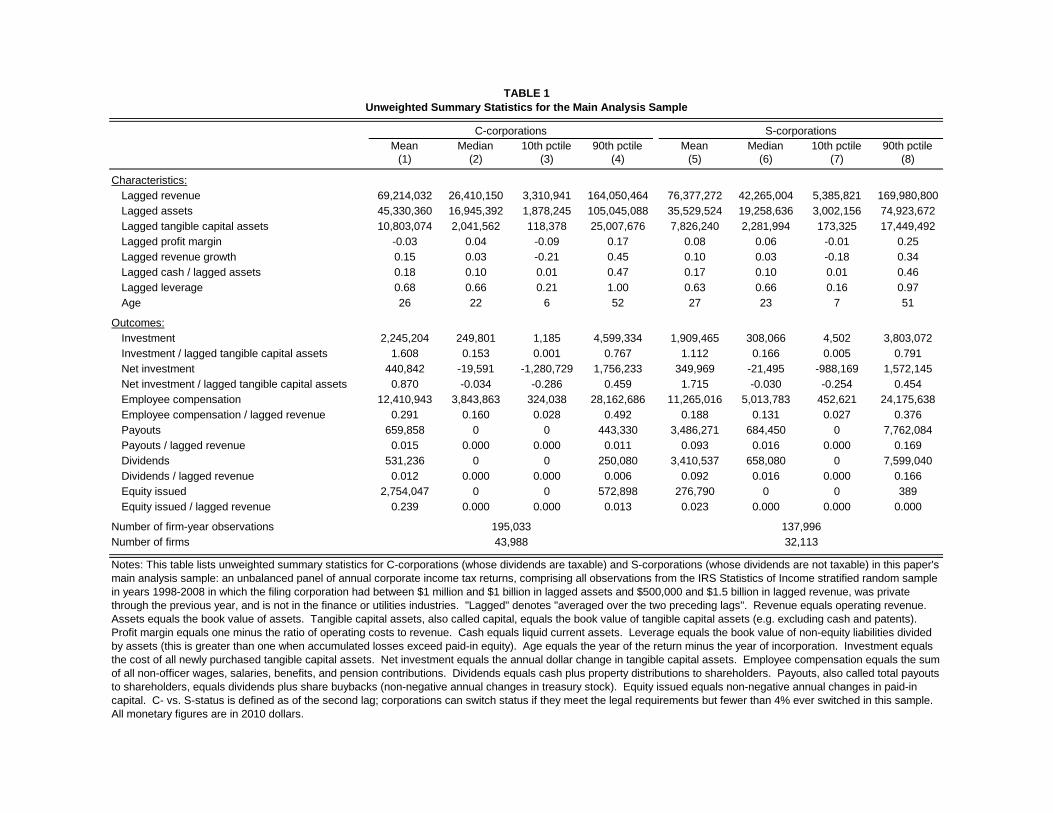
Mean Median 10th pctile 90th pctile Mean Median 10th pctile 90th pctile

(1) (2) (3) (4) (5) (6) (7) (8)

Characteristics:

Lagged revenue 69,214,032 26,410,150 3,310,941 164,050,464 76,377,272 42,265,004 5,385,821 169,980,800

Lagged assets 45,330,360 16,945,392 1,878,245 105,045,088 35,529,524 19,258,636 3,002,156 74,923,672

Lagged tangible capital assets 10,803,074 2,041,562 118,378 25,007,676 7,826,240 2,281,994 173,325 17,449,492

Lagged profit margin -0.03 0.04 -0.09 0.17 0.08 0.06 -0.01 0.25

Lagged revenue growth 0.15 0.03 -0.21 0.45 0.10 0.03 -0.18 0.34

Lagged cash / lagged assets 0.18 0.10 0.01 0.47 0.17 0.10 0.01 0.46

Lagged leverage 0.68 0.66 0.21 1.00 0.63 0.66 0.16 0.97

Age 26 22 6 52 27 23 7 51

Outcomes:

Investment 2,245,204 249,801 1,185 4,599,334 1,909,465 308,066 4,502 3,803,072

Investment / lagged tangible capital assets 1.608 0.153 0.001 0.767 1.112 0.166 0.005 0.791

Net investment 440,842 -19,591 -1,280,729 1,756,233 349,969 -21,495 -988,169 1,572,145

Net investment / lagged tangible capital assets 0.870 -0.034 -0.286 0.459 1.715 -0.030 -0.254 0.454

Employee compensation 12,410,943 3,843,863 324,038 28,162,686 11,265,016 5,013,783 452,621 24,175,638

Employee compensation / lagged revenue 0.291 0.160 0.028 0.492 0.188 0.131 0.027 0.376

Payouts 659,858 0 0 443,330 3,486,271 684,450 0 7,762,084

Payouts / lagged revenue 0.015 0.000 0.000 0.011 0.093 0.016 0.000 0.169

Dividends 531,236 0 0 250,080 3,410,537 658,080 0 7,599,040

Dividends / lagged revenue 0.012 0.000 0.000 0.006 0.092 0.016 0.000 0.166

Equity issued 2,754,047 0 0 572,898 276,790 0 0 389

Equity issued / lagged revenue 0.239 0.000 0.000 0.013 0.023 0.000 0.000 0.000

Number of firm-year observations

Number of firms

Notes: This table lists unweighted summary statistics for C-corporations (whose dividends are taxable) and S-corporations (whose dividends are not taxable) in this paper's

main analysis sample: an unbalanced panel of annual corporate income tax returns, comprising all observations from the IRS Statistics of Income stratified random sample

in years 1998-2008 in which the filing corporation had between $1 million and $1 billion in lagged assets and $500,000 and $1.5 billion in lagged revenue, was private

through the previous year, and is not in the finance or utilities industries. "Lagged" denotes "averaged over the two preceding lags". Revenue equals operating revenue.

Assets equals the book value of assets. Tangible capital assets, also called capital, equals the book value of tangible capital assets (e.g. excluding cash and patents).

Profit margin equals one minus the ratio of operating costs to revenue. Cash equals liquid current assets. Leverage equals the book value of non-equity liabilities divided

by assets (this is greater than one when accumulated losses exceed paid-in equity). Age equals the year of the return minus the year of incorporation. Investment equals

the cost of all newly purchased tangible capital assets. Net investment equals the annual dollar change in tangible capital assets. Employee compensation equals the sum

of all non-officer wages, salaries, benefits, and pension contributions. Dividends equals cash plus property distributions to shareholders. Payouts, also called total payouts

to shareholders, equals dividends plus share buybacks (non-negative annual changes in treasury stock). Equity issued equals non-negative annual changes in paid-in

capital. C- vs. S-status is defined as of the second lag; corporations can switch status if they meet the legal requirements but fewer than 4% ever switched in this sample.

All monetary figures are in 2010 dollars.

TABLE 1

Unweighted Summary Statistics for the Main Analysis Sample

C-corporations S-corporations

195,033 137,996

43,988 32,113

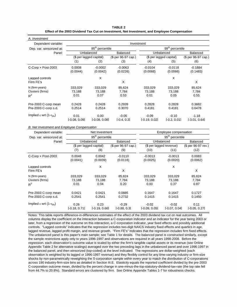
A. Investment

Dependent variable:

Dep. var. winsorized at:

Panel: Balanced Balanced

($ per 96-97 cap.) ($ per 96-97 cap.)

(1) (2) (3) (4) (5) (6)

C-Corp × Post-2003 0.0008 -0.0002 -0.0063 -0.0104 -0.0118 -0.1884

(0.0044) (0.0042) (0.0226) (0.0068) (0.0066) (0.1483)

Lagged controls X X

Firm FE's X X

N (firm-years) 333,029 333,029 85,624 333,029 333,029 85,624Clusters (firms) 73,188 73,188 7,784 73,188 73,188 7,784

R2 0.01 0.07 0.53 0.01 0.05 0.55

Pre-2003 C-corp mean 0.2428 0.2428 0.2939 0.2828 0.2828 0.3682

Pre-2003 C-corp s.d. 0.2514 0.2514 0.3070 0.4181 0.4181 0.6478

0.01 0.00 -0.05 -0.09 -0.10 -1.18

[-0.08, 0.09] [-0.08, 0.08] [-0.4, 0.3] [-0.19, 0.02] [-0.2, 0.01] [-3.01, 0.64]

B. Net Investment and Employee Compensation

Dependent variable:

Dep. var. winsorized at:

Panel: Balanced Balanced

($ per 96-97 cap.) ($ per 96-97 rev.)

(7) (8) (9) (10) (11) (12)

C-Corp × Post-2003 0.0048 0.0042 -0.0110 -0.0013 -0.0013 0.0083

(0.0041) (0.0039) (0.0116) (0.0025) (0.0020) (0.0062)

Lagged controls X X

Firm FE's X X

N (firm-years) 333,029 333,029 85,624 333,029 333,029 85,624Clusters (firms) 73,188 73,188 7,784 73,188 73,188 7,784

R2 0.01 0.04 0.20 0.00 0.37 0.87

Pre-2003 C-corp mean 0.0421 0.0421 0.0885 0.1647 0.1647 0.1727

Pre-2003 C-corp s.d. 0.2541 0.2541 0.2732 0.1415 0.1415 0.1450

0.26 0.23 -0.29 -0.02 -0.02 0.11

[-0.18, 0.71] [-0.19, 0.66] [-0.88, 0.3] [-0.09, 0.05] [-0.07, 0.04] [-0.05, 0.27]

Notes: This table reports difference-in-differences estimates of the effect of the 2003 dividend tax cut on real outcomes. All

columns display the coefficient on the interaction between a C-corporation indicator and an indicator for the year being 2003 or

later, from a regression of the outcome on this interaction, a C-corporation indicator, year fixed effects and possibly additional

controls. "Lagged controls" indicates that the regression includes two-digit NAICS industry fixed effects and quartics in age,

lagged revenue, lagged profit margin, and revenue growth. "Firm FE's" indicates that the regression includes firm fixed effects.

The unbalanced panel is this paper's main sample; see Table 1 for details. The balanced panel is constructed similarly, except

the sample restrictions apply only to years 1996-1997 and observations are required in all years 1998-2008. Before the

regression, each observation's outcome value is scaled by either the firm's tangible capital assets or its revenue (see Online

Appendix Table 2 for alternative scalings) averaged over the two preceding lags in the unbalanced panel and over 1996-1997 in

the balanced panel, and then winsorized (top-coded) at the level indicated. The regressions are dollar-weighted (each

observation is weighted by its lagged or 1996-1997 revenue) and they flexibly control for any time-varying industry or firm-size

shocks by non-parametrically reweighting the S-corporation sample within every year to match the distribution of C-corporations

across 190 industry-firm-size bins as detailed in Section III.E. Elasticity equals the reported coefficient divided by the pre-2003

C-corporation outcome mean, divided by the percent change in one-minus-the-top-statutory-dividend-tax-rate (the top rate fell

from 44.7% to 20.8%). Standard errors are clustered by firm. See Online Appendix Tables 1-7 for robustness checks.

($ per lagged capital)

Implied ε wrt (1-τdiv)

Investment

99th

percentile

Unbalanced

95th

percentile

($ per lagged revenue)

($ per lagged capital)

Implied ε wrt (1-τdiv)

Net Investment Employee compensation

Unbalanced Unbalanced

95th

percentile 95th

percentile

Unbalanced

($ per lagged capital)

TABLE 2

Effect of the 2003 Dividend Tax Cut on Investment, Net Investment, and Employee Compensation

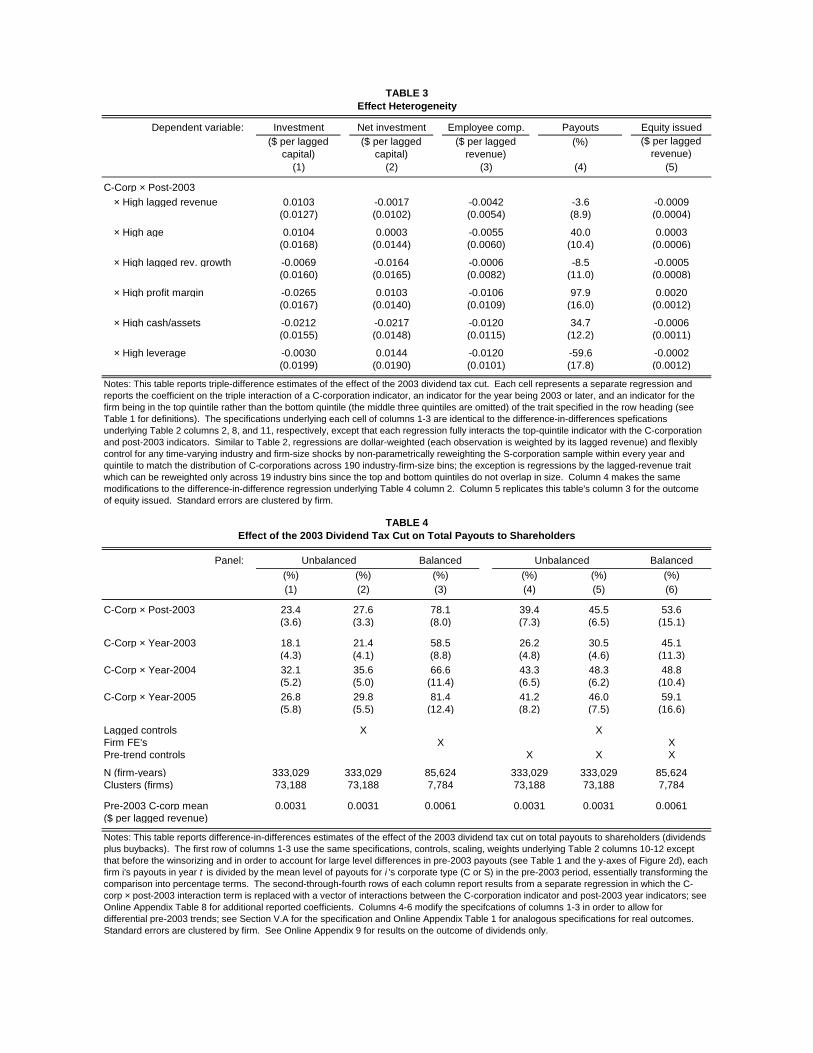
Dependent variable: Equity issued

($ per lagged

revenue)

(5)

C-Corp × Post-2003

× High lagged revenue -0.0009

(0.0004)

× High age 0.0003

(0.0006)

× High lagged rev. growth -0.0005

(0.0008)

× High profit margin 0.0020

(0.0012)

× High cash/assets -0.0006

(0.0011)

× High leverage -0.0002

(0.0012)

Panel: Balanced

(%) (%)

(1) (6)

C-Corp × Post-2003 23.4 53.6

(3.6) (15.1)

C-Corp × Year-2003 18.1 45.1

(4.3) (11.3)

C-Corp × Year-2004 32.1 48.8

(5.2) (10.4)

C-Corp × Year-2005 26.8 59.1

(5.8) (16.6)

Lagged controls

Firm FE's X

Pre-trend controls X

N (firm-years) 333,029 85,624

Clusters (firms) 73,188 7,784

Pre-2003 C-corp mean 0.0031 0.0061

($ per lagged revenue)

73,188

0.0031

41.2

(4.6)

333,029

73,188

0.00310.0031

29.8

(5.5)

X

27.6

(3.3)

21.4

(4.1)

(0.0155)

0.0144

(0.0190)

(%)

0.0103

(0.0140)

TABLE 4

(0.0101)

(%)

Unbalanced Balanced

Investment

($ per lagged

capital)

(1)

333,029

73,188

35.6

(5.0)

-0.0017

(0.0102)

0.0104

(0.0168)

39.4

(7.3)

-59.6

(17.8)

(%)

(4)

-0.0106

(0.0109)

(%)

(2)

-0.0265

(0.0167)

-0.0120

(0.0115)

-3.6

Effect of the 2003 Dividend Tax Cut on Total Payouts to Shareholders

X

0.0061

(7.5)

X

X

0.0103

(0.0127)

-0.0030

(0.0199)

-0.0212

Unbalanced

85,624

-0.0217

(0.0148)

34.7

(12.2)

X

(4.8)

43.3

(6.5)

26.2

(8.2)

(5)

333,029

TABLE 3

Effect Heterogeneity

Notes: This table reports triple-difference estimates of the effect of the 2003 dividend tax cut. Each cell represents a separate regression and

reports the coefficient on the triple interaction of a C-corporation indicator, an indicator for the year being 2003 or later, and an indicator for the

firm being in the top quintile rather than the bottom quintile (the middle three quintiles are omitted) of the trait specified in the row heading (see

Table 1 for definitions). The specifications underlying each cell of columns 1-3 are identical to the difference-in-differences spefications

underlying Table 2 columns 2, 8, and 11, respectively, except that each regression fully interacts the top-quintile indicator with the C-corporation

and post-2003 indicators. Similar to Table 2, regressions are dollar-weighted (each observation is weighted by its lagged revenue) and flexibly

control for any time-varying industry and firm-size shocks by non-parametrically reweighting the S-corporation sample within every year and

quintile to match the distribution of C-corporations across 190 industry-firm-size bins; the exception is regressions by the lagged-revenue trait

which can be reweighted only across 19 industry bins since the top and bottom quintiles do not overlap in size. Column 4 makes the same

modifications to the difference-in-difference regression underlying Table 4 column 2. Column 5 replicates this table's column 3 for the outcome

of equity issued. Standard errors are clustered by firm.

-0.0006

(0.0082)

(8.9)

97.9

(16.0)

40.0

(10.4)

-8.5

(11.0)

Payouts

(%)

-0.0069

(0.0160)

Net investment

($ per lagged

capital)

(2)

7,784

(8.8)

66.6

-0.0120

0.0003

(0.0144)

-0.0164

(0.0165)

(3)

78.1

(8.0)

(12.4)

(11.4)

Employee comp.

($ per lagged

revenue)

(3)

-0.0042

(0.0054)

-0.0055

(0.0060)

(4)

Notes: This table reports difference-in-differences estimates of the effect of the 2003 dividend tax cut on total payouts to shareholders (dividends

plus buybacks). The first row of columns 1-3 use the same specifications, controls, scaling, weights underlying Table 2 columns 10-12 except

that before the winsorizing and in order to account for large level differences in pre-2003 payouts (see Table 1 and the y-axes of Figure 2d), each

firm i's payouts in year t is divided by the mean level of payouts for i 's corporate type (C or S) in the pre-2003 period, essentially transforming the

comparison into percentage terms. The second-through-fourth rows of each column report results from a separate regression in which the C-

corp × post-2003 interaction term is replaced with a vector of interactions between the C-corporation indicator and post-2003 year indicators; see

Online Appendix Table 8 for additional reported coefficients. Columns 4-6 modify the specifcations of columns 1-3 in order to allow for

differential pre-2003 trends; see Section V.A for the specification and Online Appendix Table 1 for analogous specifications for real outcomes.

Standard errors are clustered by firm. See Online Appendix 9 for results on the outcome of dividends only.

48.3

(6.2)

46.0

45.5

(6.5)

30.5

81.4

58.5

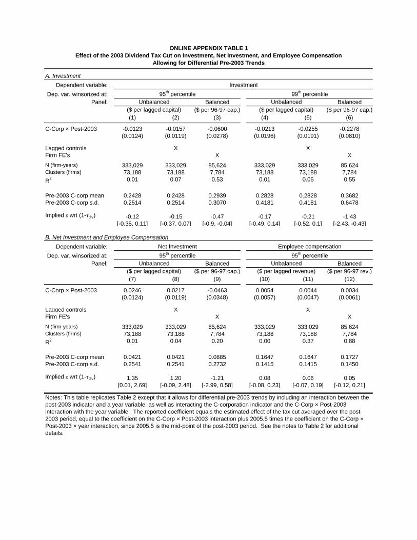
A. Investment

Dependent variable:

Dep. var. winsorized at:

Panel: Balanced Balanced

($ per 96-97 cap.) ($ per 96-97 cap.)

(1) (2) (3) (4) (5) (6)

C-Corp × Post-2003 -0.0123 -0.0157 -0.0600 -0.0213 -0.0255 -0.2278

(0.0124) (0.0119) (0.0278) (0.0196) (0.0191) (0.0810)

Lagged controls X X

Firm FE's X X

N (firm-years) 333,029 333,029 85,624 333,029 333,029 85,624Clusters (firms) 73,188 73,188 7,784 73,188 73,188 7,784

R2 0.01 0.07 0.53 0.01 0.05 0.55

Pre-2003 C-corp mean 0.2428 0.2428 0.2939 0.2828 0.2828 0.3682

Pre-2003 C-corp s.d. 0.2514 0.2514 0.3070 0.4181 0.4181 0.6478

-0.12 -0.15 -0.47 -0.17 -0.21 -1.43

[-0.35, 0.11] [-0.37, 0.07] [-0.9, -0.04] [-0.49, 0.14] [-0.52, 0.1] [-2.43, -0.43]

B. Net Investment and Employee Compensation

Dependent variable:

Dep. var. winsorized at:

Panel: Balanced Balanced

($ per 96-97 cap.) ($ per 96-97 rev.)

(7) (8) (9) (10) (11) (12)

C-Corp × Post-2003 0.0246 0.0217 -0.0463 0.0054 0.0044 0.0034

(0.0124) (0.0119) (0.0348) (0.0057) (0.0047) (0.0061)

Lagged controls X X

Firm FE's X X

N (firm-years) 333,029 333,029 85,624 333,029 333,029 85,624Clusters (firms) 73,188 73,188 7,784 73,188 73,188 7,784

R2 0.01 0.04 0.20 0.00 0.37 0.88

Pre-2003 C-corp mean 0.0421 0.0421 0.0885 0.1647 0.1647 0.1727

Pre-2003 C-corp s.d. 0.2541 0.2541 0.2732 0.1415 0.1415 0.1450

1.35 1.20 -1.21 0.08 0.06 0.05

[0.01, 2.69] [-0.09, 2.48] [-2.99, 0.58] [-0.08, 0.23] [-0.07, 0.19] [-0.12, 0.21]

Unbalanced Unbalanced

Allowing for Differential Pre-2003 Trends

ONLINE APPENDIX TABLE 1

Effect of the 2003 Dividend Tax Cut on Investment, Net Investment, and Employee Compensation

Investment

95th percentile 99

th percentile

Notes: This table replicates Table 2 except that it allows for differential pre-2003 trends by including an interaction between the

post-2003 indicator and a year variable, as well as interacting the C-corporation indicator and the C-Corp × Post-2003

interaction with the year variable. The reported coefficient equals the estimated effect of the tax cut averaged over the post-

2003 period, equal to the coefficient on the C-Corp × Post-2003 interaction plus 2005.5 times the coefficient on the C-Corp ×

Post-2003 × year interaction, since 2005.5 is the mid-point of the post-2003 period. See the notes to Table 2 for additional

details.

($ per lagged capital) ($ per lagged capital)

Implied ε wrt (1-τdiv)

Net Investment Employee compensation

95th percentile 95

th percentile

Unbalanced Unbalanced

($ per lagged capital) ($ per lagged revenue)

Implied ε wrt (1-τdiv)

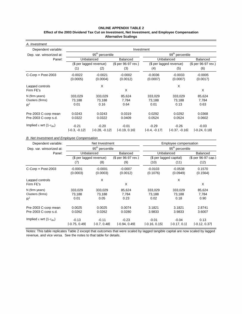
A. Investment

Dependent variable:

Dep. var. winsorized at:

Panel: Balanced Balanced

($ per 96-97 rev.) ($ per 96-97 rev.)

(1) (2) (3) (4) (5) (6)

C-Corp × Post-2003 -0.0022 -0.0021 -0.0002 -0.0036 -0.0033 -0.0005

(0.0005) (0.0004) (0.0012) (0.0007) (0.0007) (0.0017)

Lagged controls X X

Firm FE's X X

N (firm-years) 333,029 333,029 85,624 333,029 333,029 85,624Clusters (firms) 73,188 73,188 7,784 73,188 73,188 7,784

R2 0.01 0.16 0.64 0.01 0.13 0.63

Pre-2003 C-corp mean 0.0243 0.0243 0.0319 0.0292 0.0292 0.0368

Pre-2003 C-corp s.d. 0.0322 0.0322 0.0409 0.0524 0.0524 0.0602

-0.21 -0.20 -0.01 -0.29 -0.26 -0.03

[-0.3, -0.12] [-0.28, -0.12] [-0.19, 0.16] [-0.4, -0.17] [-0.37, -0.16] [-0.24, 0.18]

B. Net Investment and Employee Compensation

Dependent variable:

Dep. var. winsorized at:

Panel: Balanced Balanced

($ per 96-97 rev.) ($ per 96-97 cap.)

(7) (8) (9) (10) (11) (12)

C-Corp × Post-2003 -0.0001 -0.0001 -0.0007 -0.0103 -0.0538 0.1570

(0.0003) (0.0003) (0.0012) (0.1076) (0.0949) (0.1564)

Lagged controls X X

Firm FE's X X

N (firm-years) 333,029 333,029 85,624 333,029 333,029 85,624Clusters (firms) 73,188 73,188 7,784 73,188 73,188 7,784

R2 0.01 0.05 0.23 0.02 0.18 0.90

Pre-2003 C-corp mean 0.0025 0.0025 0.0074 3.1821 3.1821 2.8741

Pre-2003 C-corp s.d. 0.0262 0.0262 0.0280 3.9833 3.9833 3.6007

-0.13 -0.11 -0.23 -0.01 -0.04 0.13

[-0.75, 0.49] [-0.7, 0.48] [-0.94, 0.49] [-0.16, 0.15] [-0.17, 0.1] [-0.12, 0.37]

Notes: This table replicates Table 2 except that outcomes that were scaled by lagged tangible capital are now scaled by lagged

revenue, and vice versa. See the notes to that table for details.

($ per lagged revenue) ($ per lagged revenue)

Implied ε wrt (1-τdiv)

Net Investment Employee compensation

95th percentile 95

th percentile

Unbalanced Unbalanced

($ per lagged revenue) ($ per lagged capital)

Implied ε wrt (1-τdiv)

Unbalanced Unbalanced

Alternative Scalings

ONLINE APPENDIX TABLE 2

Effect of the 2003 Dividend Tax Cut on Investment, Net Investment, and Employee Compensation

Investment

95th percentile 99

th percentile

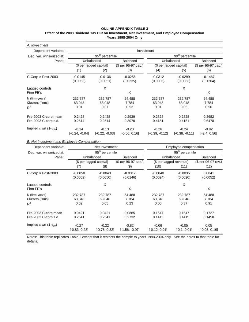
A. Investment

Dependent variable:

Dep. var. winsorized at:

Panel: Balanced Balanced

($ per 96-97 cap.) ($ per 96-97 cap.)

(1) (2) (3) (4) (5) (6)

C-Corp × Post-2003 -0.0145 -0.0136 -0.0256 -0.0312 -0.0299 -0.1467

(0.0053) (0.0051) (0.0235) (0.0085) (0.0083) (0.1204)

Lagged controls X X

Firm FE's X X

N (firm-years) 232,787 232,787 54,488 232,787 232,787 54,488Clusters (firms) 63,048 63,048 7,784 63,048 63,048 7,784

R2 0.01 0.07 0.52 0.01 0.05 0.50

Pre-2003 C-corp mean 0.2428 0.2428 0.2939 0.2828 0.2828 0.3682

Pre-2003 C-corp s.d. 0.2514 0.2514 0.3070 0.4181 0.4181 0.6478

-0.14 -0.13 -0.20 -0.26 -0.24 -0.92

[-0.24, -0.04] [-0.22, -0.03] [-0.56, 0.16] [-0.39, -0.12] [-0.38, -0.11] [-2.4, 0.56]

B. Net Investment and Employee Compensation

Dependent variable:

Dep. var. winsorized at:

Panel: Balanced Balanced

($ per 96-97 cap.) ($ per 96-97 rev.)

(7) (8) (9) (10) (11) (12)

C-Corp × Post-2003 -0.0050 -0.0040 -0.0312 -0.0040 -0.0035 0.0041

(0.0052) (0.0050) (0.0146) (0.0024) (0.0020) (0.0052)

Lagged controls X X

Firm FE's X X

N (firm-years) 232,787 232,787 54,488 232,787 232,787 54,488Clusters (firms) 63,048 63,048 7,784 63,048 63,048 7,784

R2 0.02 0.05 0.23 0.00 0.37 0.91

Pre-2003 C-corp mean 0.0421 0.0421 0.0885 0.1647 0.1647 0.1727

Pre-2003 C-corp s.d. 0.2541 0.2541 0.2732 0.1415 0.1415 0.1450

-0.27 -0.22 -0.82 -0.06 -0.05 0.05

[-0.83, 0.28] [-0.76, 0.32] [-1.56, -0.07] [-0.12, 0.01] [-0.1, 0.01] [-0.08, 0.19]

Net Investment Employee compensation

ONLINE APPENDIX TABLE 3

Effect of the 2003 Dividend Tax Cut on Investment, Net Investment, and Employee Compensation

Years 1998-2004 Only

Investment

95th percentile 99

th percentile

Unbalanced Unbalanced

($ per lagged capital) ($ per lagged capital)

Implied ε wrt (1-τdiv)

Implied ε wrt (1-τdiv)

Notes: This table replicates Table 2 except that it restricts the sample to years 1998-2004 only. See the notes to that table for

details.

95th percentile 95

th percentile

Unbalanced Unbalanced

($ per lagged capital) ($ per lagged revenue)

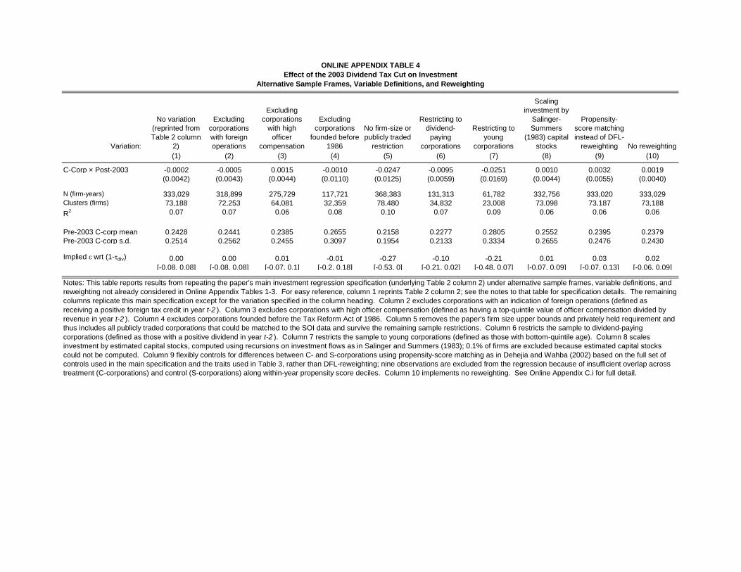
Variation:

No variation

(reprinted from

Table 2 column

2)

Excluding

corporations

with foreign

operations

Excluding

corporations

with high

officer

compensation

Excluding

corporations

founded before

1986

No firm-size or

publicly traded

restriction

Restricting to

dividend-

paying

corporations

Restricting to

young

corporations

Scaling

investment by

Salinger-

Summers

(1983) capital

stocks

Propensity-

score matching

instead of DFL-

reweighting No reweighting

(1) (2) (3) (4) (5) (6) (7) (8) (9) (10)

C-Corp × Post-2003 -0.0002 -0.0005 0.0015 -0.0010 -0.0247 -0.0095 -0.0251 0.0010 0.0032 0.0019

(0.0042) (0.0043) (0.0044) (0.0110) (0.0125) (0.0059) (0.0169) (0.0044) (0.0055) (0.0040)

N (firm-years) 333,029 318,899 275,729 117,721 368,383 131,313 61,782 332,756 333,020 333,029Clusters (firms) 73,188 72,253 64,081 32,359 78,480 34,832 23,008 73,098 73,187 73,188

R2 0.07 0.07 0.06 0.08 0.10 0.07 0.09 0.06 0.06 0.06

Pre-2003 C-corp mean 0.2428 0.2441 0.2385 0.2655 0.2158 0.2277 0.2805 0.2552 0.2395 0.2379

Pre-2003 C-corp s.d. 0.2514 0.2562 0.2455 0.3097 0.1954 0.2133 0.3334 0.2655 0.2476 0.2430

0.00 0.00 0.01 -0.01 -0.27 -0.10 -0.21 0.01 0.03 0.02

[-0.08, 0.08] [-0.08, 0.08] [-0.07, 0.1] [-0.2, 0.18] [-0.53, 0] [-0.21, 0.02] [-0.48, 0.07] [-0.07, 0.09] [-0.07, 0.13] [-0.06, 0.09]

Notes: This table reports results from repeating the paper's main investment regression specification (underlying Table 2 column 2) under alternative sample frames, variable definitions, and

reweighting not already considered in Online Appendix Tables 1-3. For easy reference, column 1 reprints Table 2 column 2; see the notes to that table for specification details. The remaining

columns replicate this main specification except for the variation specified in the column heading. Column 2 excludes corporations with an indication of foreign operations (defined as

receiving a positive foreign tax credit in year t-2 ). Column 3 excludes corporations with high officer compensation (defined as having a top-quintile value of officer compensation divided by

revenue in year t-2 ). Column 4 excludes corporations founded before the Tax Reform Act of 1986. Column 5 removes the paper's firm size upper bounds and privately held requirement and

thus includes all publicly traded corporations that could be matched to the SOI data and survive the remaining sample restrictions. Column 6 restricts the sample to dividend-paying

corporations (defined as those with a positive dividend in year t-2 ). Column 7 restricts the sample to young corporations (defined as those with bottom-quintile age). Column 8 scales

investment by estimated capital stocks, computed using recursions on investment flows as in Salinger and Summers (1983); 0.1% of firms are excluded because estimated capital stocks

could not be computed. Column 9 flexibly controls for differences between C- and S-corporations using propensity-score matching as in Dehejia and Wahba (2002) based on the full set of

controls used in the main specification and the traits used in Table 3, rather than DFL-reweighting; nine observations are excluded from the regression because of insufficient overlap across

treatment (C-corporations) and control (S-corporations) along within-year propensity score deciles. Column 10 implements no reweighting. See Online Appendix C.i for full detail.

Implied ε wrt (1-τdiv)

ONLINE APPENDIX TABLE 4

Effect of the 2003 Dividend Tax Cut on Investment

Alternative Sample Frames, Variable Definitions, and Reweighting

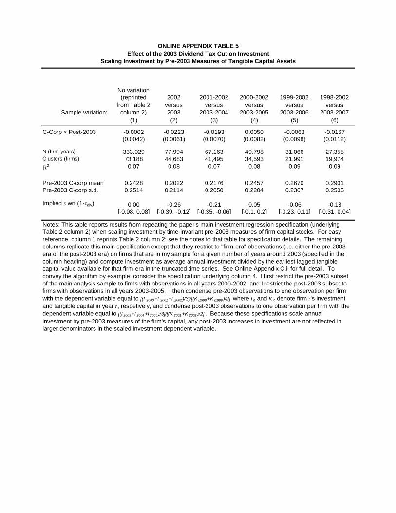
Sample variation:

No variation

(reprinted

from Table 2

column 2)

2002

versus

2003

2001-2002

versus

2003-2004

2000-2002

versus

2003-2005

1999-2002

versus

2003-2006

1998-2002

versus

2003-2007

(1) (2) (3) (4) (5) (6)

C-Corp × Post-2003 -0.0002 -0.0223 -0.0193 0.0050 -0.0068 -0.0167

(0.0042) (0.0061) (0.0070) (0.0082) (0.0098) (0.0112)

N (firm-years) 333,029 77,994 67,163 49,798 31,066 27,355Clusters (firms) 73,188 44,683 41,495 34,593 21,991 19,974

R2 0.07 0.08 0.07 0.08 0.09 0.09

Pre-2003 C-corp mean 0.2428 0.2022 0.2176 0.2457 0.2670 0.2901

Pre-2003 C-corp s.d. 0.2514 0.2114 0.2050 0.2204 0.2367 0.2505

0.00 -0.26 -0.21 0.05 -0.06 -0.13

[-0.08, 0.08] [-0.39, -0.12] [-0.35, -0.06] [-0.1, 0.2] [-0.23, 0.11] [-0.31, 0.04]

ONLINE APPENDIX TABLE 5

Effect of the 2003 Dividend Tax Cut on Investment

Scaling Investment by Pre-2003 Measures of Tangible Capital Assets

Implied ε wrt (1-τdiv)

Notes: This table reports results from repeating the paper's main investment regression specification (underlying

Table 2 column 2) when scaling investment by time-invariant pre-2003 measures of firm capital stocks. For easy

reference, column 1 reprints Table 2 column 2; see the notes to that table for specification details. The remaining

columns replicate this main specification except that they restrict to "firm-era" observations (i.e. either the pre-2003

era or the post-2003 era) on firms that are in my sample for a given number of years around 2003 (specified in the

column heading) and compute investment as average annual investment divided by the earliest lagged tangible

capital value available for that firm-era in the truncated time series. See Online Appendix C.ii for full detail. To

convey the algorithm by example, consider the specification underlying column 4. I first restrict the pre-2003 subset

of the main analysis sample to firms with observations in all years 2000-2002, and I restrict the post-2003 subset to

firms with observations in all years 2003-2005. I then condense pre-2003 observations to one observation per firm

with the dependent variable equal to [(I i2000 +I i2001 +I i2002 )/3]/[(K i1998 +K i1999 )/2] where I it and K it denote firm i 's investment

and tangible capital in year t , respetively, and condense post-2003 observations to one observation per firm with the

dependent variable equal to [(I 2003 +I 2004 +I 2005 )/3]/[(K 2001 +K 2002 )/2] . Because these specifications scale annual

investment by pre-2003 measures of the firm's capital, any post-2003 increases in investment are not reflected in

larger denominators in the scaled investment dependent variable.

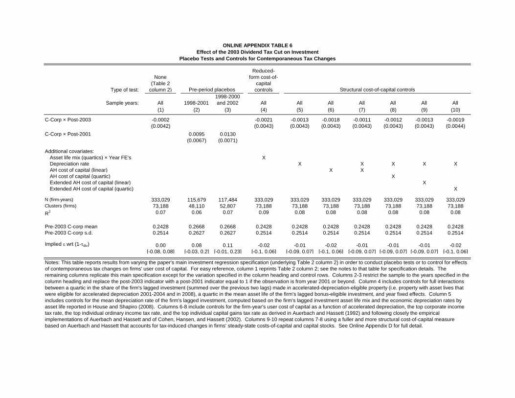
Type of test:

None

(Table 2

column 2)

Reduced-

form cost-of-

capital

controls

Sample years: All 1998-2001

1998-2000

and 2002 All All All All All All All

(1) (2) (3) (4) (5) (6) (7) (8) (9) (10)

C-Corp × Post-2003 -0.0002 -0.0021 -0.0013 -0.0018 -0.0011 -0.0012 -0.0013 -0.0019

(0.0042) (0.0043) (0.0043) (0.0043) (0.0043) (0.0043) (0.0043) (0.0044)

C-Corp × Post-2001 0.0095 0.0130

(0.0067) (0.0071)

Additional covariates:

Asset life mix (quartics) × Year FE's X

Depreciation rate X X X X X

AH cost of capital (linear) X X

AH cost of capital (quartic) X

Extended AH cost of capital (linear) X

Extended AH cost of capital (quartic) X

N (firm-years) 333,029 115,679 117,484 333,029 333,029 333,029 333,029 333,029 333,029 333,029Clusters (firms) 73,188 48,110 52,807 73,188 73,188 73,188 73,188 73,188 73,188 73,188

R2 0.07 0.06 0.07 0.09 0.08 0.08 0.08 0.08 0.08 0.08

Pre-2003 C-corp mean 0.2428 0.2668 0.2668 0.2428 0.2428 0.2428 0.2428 0.2428 0.2428 0.2428

Pre-2003 C-corp s.d. 0.2514 0.2627 0.2627 0.2514 0.2514 0.2514 0.2514 0.2514 0.2514 0.2514

0.00 0.08 0.11 -0.02 -0.01 -0.02 -0.01 -0.01 -0.01 -0.02

[-0.08, 0.08] [-0.03, 0.2] [-0.01, 0.23] [-0.1, 0.06] [-0.09, 0.07] [-0.1, 0.06] [-0.09, 0.07] [-0.09, 0.07] [-0.09, 0.07] [-0.1, 0.06]

Notes: This table reports results from varying the paper's main investment regression specification (underlying Table 2 column 2) in order to conduct placebo tests or to control for effects

of contemporaneous tax changes on firms' user cost of capital. For easy reference, column 1 reprints Table 2 column 2; see the notes to that table for specification details. The

remaining columns replicate this main specification except for the variation specified in the column heading and control rows. Columns 2-3 restrict the sample to the years specified in the

column heading and replace the post-2003 indicator with a post-2001 indicator equal to 1 if the observation is from year 2001 or beyond. Column 4 includes controls for full interactions

between a quartic in the share of the firm's lagged investment (summed over the previous two lags) made in accelerated-depreciation-eligible property (i.e. property with asset lives that

were eligible for accelerated depreciation 2001-2004 and in 2008), a quartic in the mean asset life of the firm's lagged bonus-eligible investment, and year fixed effects. Column 5

includes controls for the mean depreciation rate of the firm's lagged investment, computed based on the firm's lagged investment asset life mix and the economic depreciation rates by

asset life reported in House and Shapiro (2008). Columns 6-8 include controls for the firm-year's user cost of capital as a function of accelerated depreciation, the top corporate income

tax rate, the top individual ordinary income tax rate, and the top individual capital gains tax rate as derived in Auerbach and Hassett (1992) and following closely the empirical

implementations of Auerbach and Hassett and of Cohen, Hansen, and Hassett (2002). Columns 9-10 repeat columns 7-8 using a fuller and more structural cost-of-capital measure

based on Auerbach and Hassett that accounts for tax-induced changes in firms' steady-state costs-of-capital and capital stocks. See Online Appendix D for full detail.

Pre-period placebos

ONLINE APPENDIX TABLE 6

Effect of the 2003 Dividend Tax Cut on Investment

Placebo Tests and Controls for Contemporaneous Tax Changes

Implied ε wrt (1-τdiv)

Structural cost-of-capital controls

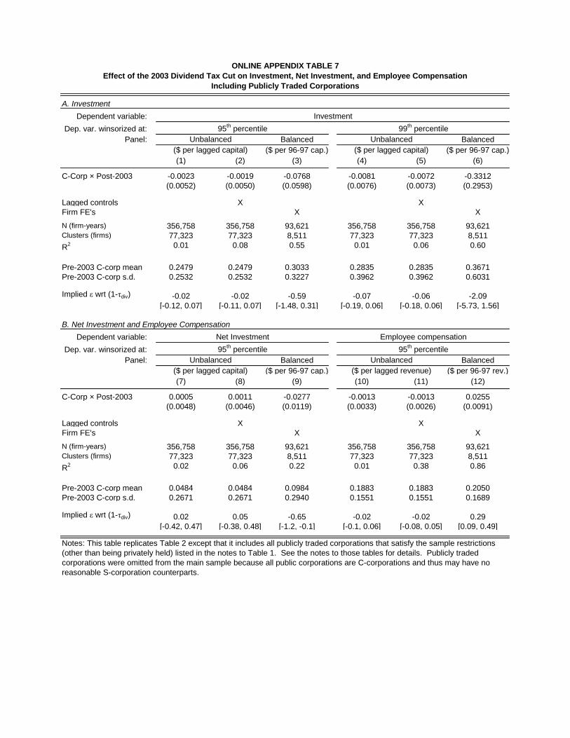
A. Investment

Dependent variable:

Dep. var. winsorized at:

Panel: Balanced Balanced

($ per 96-97 cap.) ($ per 96-97 cap.)

(1) (2) (3) (4) (5) (6)

C-Corp × Post-2003 -0.0023 -0.0019 -0.0768 -0.0081 -0.0072 -0.3312

(0.0052) (0.0050) (0.0598) (0.0076) (0.0073) (0.2953)

Lagged controls X X

Firm FE's X X

N (firm-years) 356,758 356,758 93,621 356,758 356,758 93,621Clusters (firms) 77,323 77,323 8,511 77,323 77,323 8,511

R2 0.01 0.08 0.55 0.01 0.06 0.60

Pre-2003 C-corp mean 0.2479 0.2479 0.3033 0.2835 0.2835 0.3671

Pre-2003 C-corp s.d. 0.2532 0.2532 0.3227 0.3962 0.3962 0.6031

-0.02 -0.02 -0.59 -0.07 -0.06 -2.09

[-0.12, 0.07] [-0.11, 0.07] [-1.48, 0.31] [-0.19, 0.06] [-0.18, 0.06] [-5.73, 1.56]

B. Net Investment and Employee Compensation

Dependent variable:

Dep. var. winsorized at:

Panel: Balanced Balanced

($ per 96-97 cap.) ($ per 96-97 rev.)

(7) (8) (9) (10) (11) (12)

C-Corp × Post-2003 0.0005 0.0011 -0.0277 -0.0013 -0.0013 0.0255

(0.0048) (0.0046) (0.0119) (0.0033) (0.0026) (0.0091)

Lagged controls X X

Firm FE's X X

N (firm-years) 356,758 356,758 93,621 356,758 356,758 93,621Clusters (firms) 77,323 77,323 8,511 77,323 77,323 8,511

R2 0.02 0.06 0.22 0.01 0.38 0.86

Pre-2003 C-corp mean 0.0484 0.0484 0.0984 0.1883 0.1883 0.2050

Pre-2003 C-corp s.d. 0.2671 0.2671 0.2940 0.1551 0.1551 0.1689

0.02 0.05 -0.65 -0.02 -0.02 0.29

[-0.42, 0.47] [-0.38, 0.48] [-1.2, -0.1] [-0.1, 0.06] [-0.08, 0.05] [0.09, 0.49]

Unbalanced Unbalanced

Including Publicly Traded Corporations

ONLINE APPENDIX TABLE 7

Effect of the 2003 Dividend Tax Cut on Investment, Net Investment, and Employee Compensation

Investment

95th percentile 99

th percentile

Notes: This table replicates Table 2 except that it includes all publicly traded corporations that satisfy the sample restrictions

(other than being privately held) listed in the notes to Table 1. See the notes to those tables for details. Publicly traded

corporations were omitted from the main sample because all public corporations are C-corporations and thus may have no

reasonable S-corporation counterparts.

($ per lagged capital) ($ per lagged capital)

Implied ε wrt (1-τdiv)

Net Investment Employee compensation

95th percentile 95

th percentile

Unbalanced Unbalanced

($ per lagged capital) ($ per lagged revenue)

Implied ε wrt (1-τdiv)

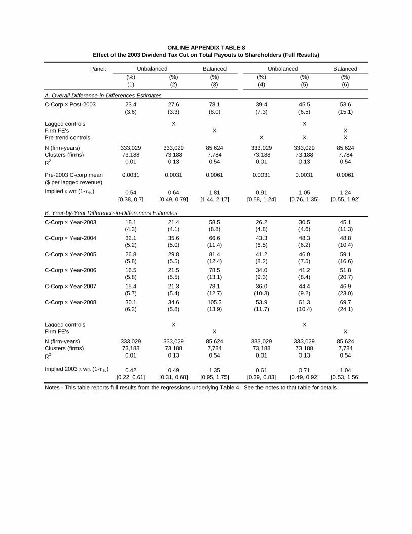
Panel: Balanced Balanced

(%) (%) (%) (%) (%) (%)

(1) (2) (3) (4) (5) (6)

A. Overall Difference-in-Differences Estimates

C-Corp × Post-2003 23.4 27.6 78.1 39.4 45.5 53.6

(3.6) (3.3) (8.0) (7.3) (6.5) (15.1)

Lagged controls X X

Firm FE's X X

Pre-trend controls X X X

N (firm-years) 333,029 333,029 85,624 333,029 333,029 85,624

Clusters (firms) 73,188 73,188 7,784 73,188 73,188 7,784

R2 0.01 0.13 0.54 0.01 0.13 0.54

Pre-2003 C-corp mean 0.0031 0.0031 0.0061 0.0031 0.0031 0.0061

($ per lagged revenue)

0.54 0.64 1.81 0.91 1.05 1.24

[0.38, 0.7] [0.49, 0.79] [1.44, 2.17] [0.58, 1.24] [0.76, 1.35] [0.55, 1.92]

B. Year-by-Year Difference-in-Differences Estimates

C-Corp × Year-2003 18.1 21.4 58.5 26.2 30.5 45.1

(4.3) (4.1) (8.8) (4.8) (4.6) (11.3)

C-Corp × Year-2004 32.1 35.6 66.6 43.3 48.3 48.8

(5.2) (5.0) (11.4) (6.5) (6.2) (10.4)

C-Corp × Year-2005 26.8 29.8 81.4 41.2 46.0 59.1

(5.8) (5.5) (12.4) (8.2) (7.5) (16.6)

C-Corp × Year-2006 16.5 21.5 78.5 34.0 41.2 51.8

(5.8) (5.5) (13.1) (9.3) (8.4) (20.7)

C-Corp × Year-2007 15.4 21.3 78.1 36.0 44.4 46.9

(5.7) (5.4) (12.7) (10.3) (9.2) (23.0)

C-Corp × Year-2008 30.1 34.6 105.3 53.9 61.3 69.7

(6.2) (5.8) (13.9) (11.7) (10.4) (24.1)

Lagged controls X X

Firm FE's X X

N (firm-years) 333,029 333,029 85,624 333,029 333,029 85,624

Clusters (firms) 73,188 73,188 7,784 73,188 73,188 7,784

R2 0.01 0.13 0.54 0.01 0.13 0.54

0.42 0.49 1.35 0.61 0.71 1.04

[0.22, 0.61] [0.31, 0.68] [0.95, 1.75] [0.39, 0.83] [0.49, 0.92] [0.53, 1.56]

Implied ε wrt (1-τdiv)

Notes - This table reports full results from the regressions underlying Table 4. See the notes to that table for details.

Implied 2003 ε wrt (1-τdiv)

ONLINE APPENDIX TABLE 8

Effect of the 2003 Dividend Tax Cut on Total Payouts to Shareholders (Full Results)

Unbalanced Unbalanced

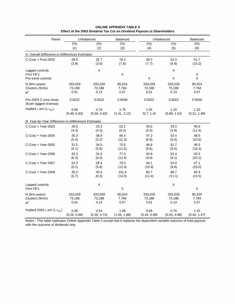
Panel: Balanced Balanced

(%) (%) (%) (%) (%) (%)

(1) (2) (3) (4) (5) (6)

A. Overall Difference-in-Differences Estimates

C-Corp × Post-2003 28.5 32.7 76.2 45.5 52.0 51.7

(3.9) (3.6) (7.8) (7.7) (6.9) (15.2)

Lagged controls X X

Firm FE's X X

Pre-trend controls X X X

N (firm-years) 333,029 333,029 85,624 333,029 333,029 85,624

Clusters (firms) 73,188 73,188 7,784 73,188 73,188 7,784

R2 0.01 0.13 0.57 0.01 0.13 0.57

Pre-2003 C-corp mean 0.0022 0.0022 0.0048 0.0022 0.0022 0.0048

($ per lagged revenue)

0.66 0.76 1.76 1.05 1.20 1.20

[0.48, 0.83] [0.59, 0.92] [1.41, 2.12] [0.7, 1.4] [0.89, 1.52] [0.51, 1.89]

B. Year-by-Year Difference-in-Differences Estimates

C-Corp × Year-2003 20.0 23.3 63.2 28.6 33.0 49.9

(4.4) (4.3) (9.2) (5.0) (4.8) (11.4)

C-Corp × Year-2004 35.3 38.9 66.4 47.2 52.4 48.5

(5.4) (5.2) (11.3) (6.8) (6.5) (10.6)

C-Corp × Year-2005 31.5 34.5 70.6 46.8 51.7 48.3

(6.1) (5.8) (11.5) (8.6) (8.0) (16.3)

C-Corp × Year-2006 26.3 31.5 77.3 44.8 52.4 50.5

(6.3) (6.0) (12.4) (9.9) (9.1) (20.2)

C-Corp × Year-2007 22.3 28.4 78.3 44.1 53.0 47.1

(6.1) (5.8) (12.4) (10.9) (9.8) (23.0)

C-Corp × Year-2008 35.5 40.3 101.6 60.7 68.7 65.9

(6.7) (6.3) (14.0) (12.4) (11.1) (24.5)

Lagged controls X X

Firm FE's X X

N (firm-years) 333,029 333,029 85,624 333,029 333,029 85,624

Clusters (firms) 73,188 73,188 7,784 73,188 73,188 7,784

R2 0.01 0.13 0.57 0.01 0.13 0.57

0.46 0.54 1.46 0.66 0.76 1.15

[0.26, 0.66] [0.35, 0.73] [1.05, 1.88] [0.44, 0.89] [0.55, 0.98] [0.64, 1.67]

Implied 2003 ε wrt (1-τdiv)

Notes - This table replicates Online Appendix Table 5 except that it replaces the dependent variable outcome of total payouts

with the outcome of dividends only.

ONLINE APPENDIX TABLE 9

Effect of the 2003 Dividend Tax Cut on Dividend Payouts to Shareholders

Unbalanced Unbalanced

Implied ε wrt (1-τdiv)

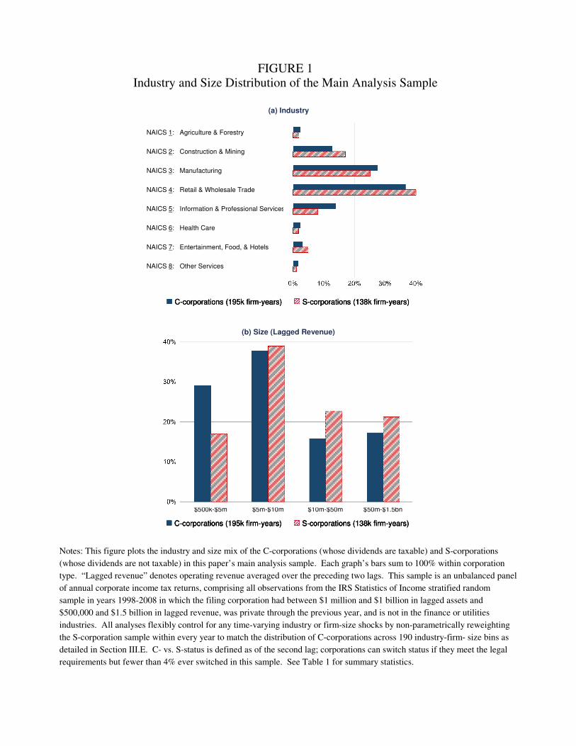
FIGURE 1Industry and Size Distribution of the Main Analysis Sample

C-corporations (195k firm-years) S-corporations (138k firm-years)C-corporations (195k firm-years)C-corporations (195k firm-years) S-corporations (138k firm-years)S-corporations (138k firm-years)

(a) Industry

NAICS 1: Agriculture & Forestry

NAICS 6: Health Care

NAICS 2: Construction & Mining

NAICS 3: Manufacturing

NAICS 4: Retail & Wholesale Trade

NAICS 5: Information & Professional Services

NAICS 7: Entertainment, Food, & Hotels

NAICS 8: Other Services

(b) Size (Lagged Revenue)

$5m-$10m$500k-$5m $10m-$50m $50m-$1.5bn

C-corporations (195k firm-years) S-corporations (138k firm-years)C-corporations (195k firm-years)C-corporations (195k firm-years) S-corporations (138k firm-years)S-corporations (138k firm-years)

Notes: This figure plots the industry and size mix of the C-corporations (whose dividends are taxable) and S-corporations

(whose dividends are not taxable) in this paper’s main analysis sample. Each graph’s bars sum to 100% within corporation

type. “Lagged revenue” denotes operating revenue averaged over the preceding two lags. This sample is an unbalanced panel

of annual corporate income tax returns, comprising all observations from the IRS Statistics of Income stratified random

sample in years 1998-2008 in which the filing corporation had between $1 million and $1 billion in lagged assets and

$500,000 and $1.5 billion in lagged revenue, was private through the previous year, and is not in the finance or utilities

industries. All analyses flexibly control for any time-varying industry or firm-size shocks by non-parametrically reweighting

the S-corporation sample within every year to match the distribution of C-corporations across 190 industry-firm- size bins as

detailed in Section III.E. C- vs. S-status is defined as of the second lag; corporations can switch status if they meet the legal

requirements but fewer than 4% ever switched in this sample. See Table 1 for summary statistics.

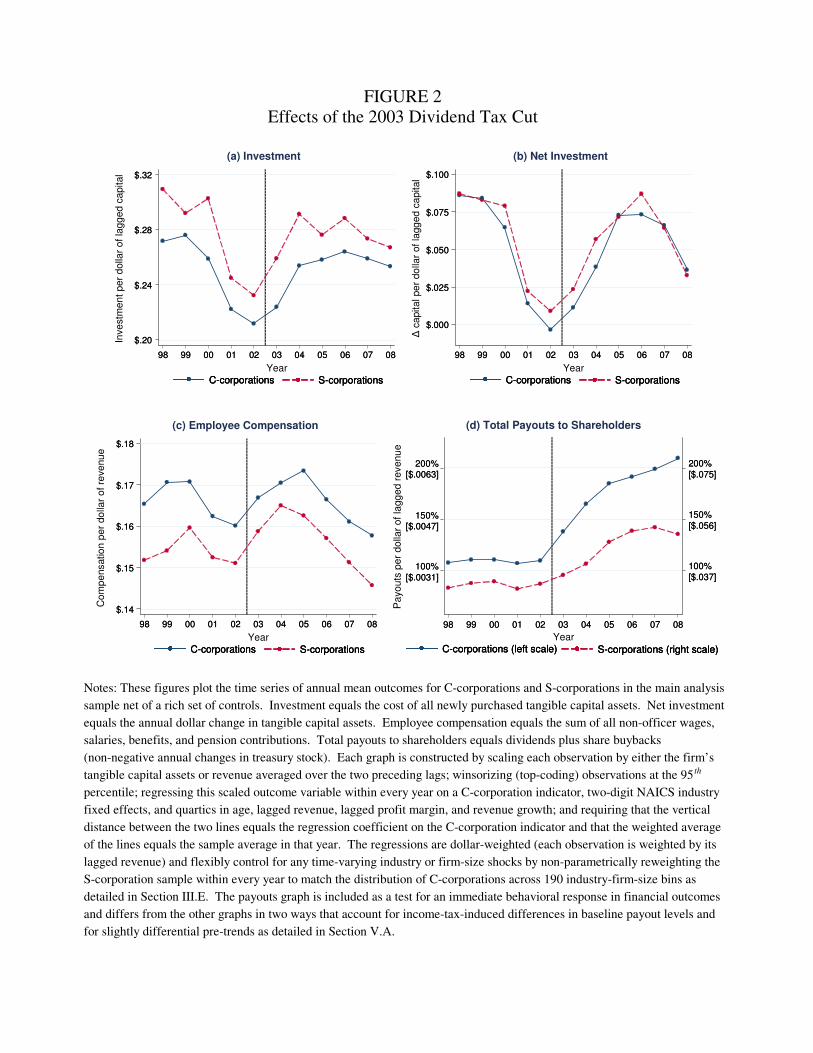
FIGURE 2Effects of the 2003 Dividend Tax Cut

(a) Investment

Year

Inve

stm

en

t pe

r d

olla

r o

f la

gg

ed c

apital

9898

$.32$.32

$.24$.24

$.20$.20

0808

$.28$.28

C-corporations S-corporationsC-corporationsC-corporations S-corporationsS-corporations

9999 0000 0101 0202 0303 0404 0505 0606 0707

Year

∆ca

pital pe

r do

llar

of

lagg

ed c

apital

C-corporations S-corporationsC-corporationsC-corporations S-corporationsS-corporations

(b) Net Investment

$.100$.100

$.050$.050

$.000$.000

$.075$.075

$.025$.025

9898 08089999 0000 0101 0202 0303 0404 0505 0606 0707

Year

Co

mp

ensatio

n p

er

do

llar

of re

ve

nu

e

C-corporations S-corporationsC-corporationsC-corporations S-corporationsS-corporations

(c) Employee Compensation

$.18$.18

$.15$.15

$.14$.14

$.16$.16

$.17$.17

9898 08089999 0000 0101 0202 0303 0404 0505 0606 0707

Year

(d) Total Payouts to Shareholders

Pa

you

ts p

er

do

llar

of

lag

ge

d r

eve

nu

e

200% [$.0063]

200% [$.0063]

200% [$.075]200% [$.075]

150% [$.056]150% [$.056]

100% [$.037]100% [$.037]

100% [$.0031]

100% [$.0031]

150% [$.0047]

150% [$.0047]

C-corporations (left scale) S-corporations (right scale)C-corporations (left scale)C-corporations (left scale) S-corporations (right scale)S-corporations (right scale)

9898 08089999 0000 0101 0202 0303 0404 0505 0606 0707

Notes: These figures plot the time series of annual mean outcomes for C-corporations and S-corporations in the main analysis

sample net of a rich set of controls. Investment equals the cost of all newly purchased tangible capital assets. Net investment

equals the annual dollar change in tangible capital assets. Employee compensation equals the sum of all non-officer wages,

salaries, benefits, and pension contributions. Total payouts to shareholders equals dividends plus share buybacks

(non-negative annual changes in treasury stock). Each graph is constructed by scaling each observation by either the firm’s

tangible capital assets or revenue averaged over the two preceding lags; winsorizing (top-coding) observations at the 95 th

percentile; regressing this scaled outcome variable within every year on a C-corporation indicator, two-digit NAICS industry

fixed effects, and quartics in age, lagged revenue, lagged profit margin, and revenue growth; and requiring that the vertical

distance between the two lines equals the regression coefficient on the C-corporation indicator and that the weighted average

of the lines equals the sample average in that year. The regressions are dollar-weighted (each observation is weighted by its

lagged revenue) and flexibly control for any time-varying industry or firm-size shocks by non-parametrically reweighting the

S-corporation sample within every year to match the distribution of C-corporations across 190 industry-firm-size bins as

detailed in Section III.E. The payouts graph is included as a test for an immediate behavioral response in financial outcomes

and differs from the other graphs in two ways that account for income-tax-induced differences in baseline payout levels and

for slightly differential pre-trends as detailed in Section V.A.

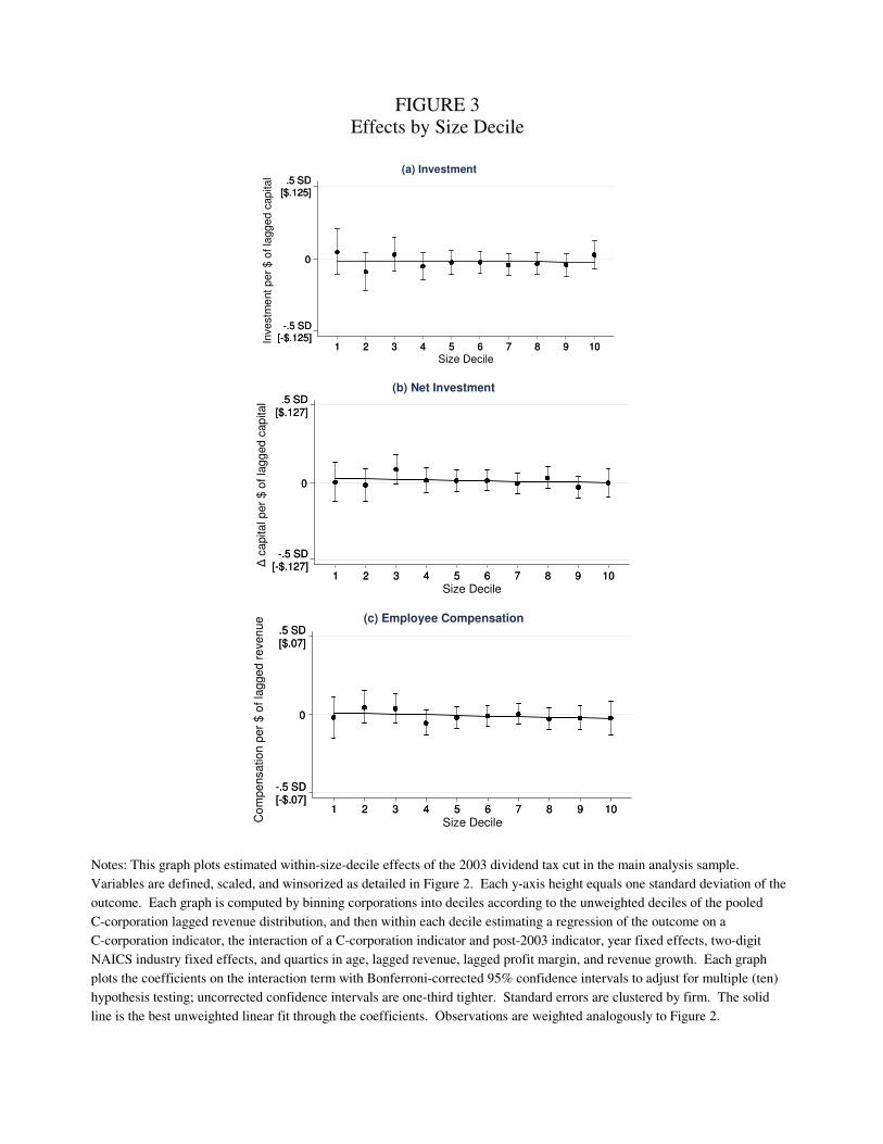
FIGURE 3Effects by Size Decile

(a) Investment

Investm

ent

per

$ o

f la

gg

ed c

ap

ital

Size Decile11 101022 33 44 55 66 77 88 99

.5 SD [$.125].5 SD

[$.125]

-.5 SD [-$.125]-.5 SD

[-$.125]

00

(b) Net Investment

∆ca

pita

l p

er

$ o

f la

gg

ed

cap

ital

Size Decile11 101022 33 44 55 66 77 88 99

.5 SD [$.127].5 SD

[$.127]

-.5 SD [-$.127]-.5 SD

[-$.127]

00

(c) Employee Compensation

Co

mpensatio

n p

er

$ o

f la

gged r

even

ue

Size Decile11 101022 33 44 55 66 77 88 99

.5 SD [$.07].5 SD [$.07]

-.5 SD [-$.07]-.5 SD [-$.07]

00

Notes: This graph plots estimated within-size-decile effects of the 2003 dividend tax cut in the main analysis sample.

Variables are defined, scaled, and winsorized as detailed in Figure 2. Each y-axis height equals one standard deviation of the

outcome. Each graph is computed by binning corporations into deciles according to the unweighted deciles of the pooled

C-corporation lagged revenue distribution, and then within each decile estimating a regression of the outcome on a

C-corporation indicator, the interaction of a C-corporation indicator and post-2003 indicator, year fixed effects, two-digit

NAICS industry fixed effects, and quartics in age, lagged revenue, lagged profit margin, and revenue growth. Each graph

plots the coefficients on the interaction term with Bonferroni-corrected 95% confidence intervals to adjust for multiple (ten)

hypothesis testing; uncorrected confidence intervals are one-third tighter. Standard errors are clustered by firm. The solid

line is the best unweighted linear fit through the coefficients. Observations are weighted analogously to Figure 2.

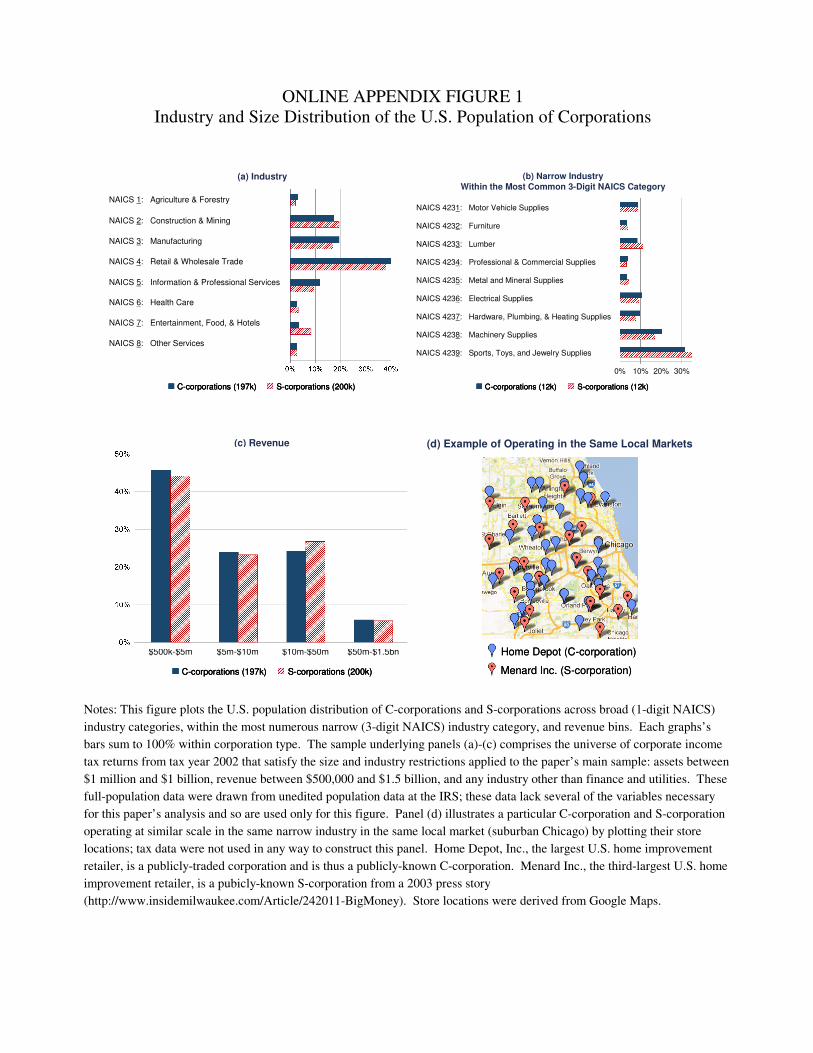
ONLINE APPENDIX FIGURE 1Industry and Size Distribution of the U.S. Population of Corporations

C-corporations (197k) S-corporations (200k)C-corporations (197k)C-corporations (197k) S-corporations (200k)S-corporations (200k)

(a) Industry

NAICS 1: Agriculture & Forestry

NAICS 6: Health Care

NAICS 2: Construction & Mining

NAICS 3: Manufacturing

NAICS 4: Retail & Wholesale Trade

NAICS 5: Information & Professional Services

NAICS 7: Entertainment, Food, & Hotels

NAICS 8: Other Services

(b) Narrow Industry

Within the Most Common 3-Digit NAICS Category

NAICS 4231: Motor Vehicle Supplies

NAICS 4236: Electrical Supplies

NAICS 4232: Furniture

NAICS 4233: Lumber

NAICS 4234: Professional & Commercial Supplies

NAICS 4235: Metal and Mineral Supplies

NAICS 4237: Hardware, Plumbing, & Heating Supplies

NAICS 4238: Machinery Supplies

NAICS 4239: Sports, Toys, and Jewelry Supplies

30%20%10%

C-corporations (12k) S-corporations (12k)C-corporations (12k)C-corporations (12k) S-corporations (12k)S-corporations (12k)

0%

(c) Revenue

$5m-$10m$500k-$5m $10m-$50m $50m-$1.5bn

C-corporations (197k) S-corporations (200k)C-corporations (197k)C-corporations (197k) S-corporations (200k)S-corporations (200k)

Home Depot (C-corporation)Home Depot (C-corporation)

(d) Example of Operating in the Same Local Markets

Menard Inc. (S-corporation)Menard Inc. (S-corporation)

Notes: This figure plots the U.S. population distribution of C-corporations and S-corporations across broad (1-digit NAICS)

industry categories, within the most numerous narrow (3-digit NAICS) industry category, and revenue bins. Each graphs’s

bars sum to 100% within corporation type. The sample underlying panels (a)-(c) comprises the universe of corporate income

tax returns from tax year 2002 that satisfy the size and industry restrictions applied to the paper’s main sample: assets between

$1 million and $1 billion, revenue between $500,000 and $1.5 billion, and any industry other than finance and utilities. These

full-population data were drawn from unedited population data at the IRS; these data lack several of the variables necessary

for this paper’s analysis and so are used only for this figure. Panel (d) illustrates a particular C-corporation and S-corporation

operating at similar scale in the same narrow industry in the same local market (suburban Chicago) by plotting their store

locations; tax data were not used in any way to construct this panel. Home Depot, Inc., the largest U.S. home improvement

retailer, is a publicly-traded corporation and is thus a publicly-known C-corporation. Menard Inc., the third-largest U.S. home

improvement retailer, is a pubicly-known S-corporation from a 2003 press story

(http://www.insidemilwaukee.com/Article/242011-BigMoney). Store locations were derived from Google Maps.