NBER WORKING PAPER SERIES

BALANCED AND UNBALANCED GROWTH

James E. Rauch

Working Paper No, 4659

NATIONALBUREAU OF ECONOMIC RESEARCH1050 Massachusetts Avenue

Cambridge, MA 02138February 1994

I thank Pu Shen for her invaluable research assistance, Andy Levin for his helpful comments,and Rudolf Buitelaar for providing me with data from the files of ECLAC. I am also gratefulfor research assistance provided by Subir Bose, Brad Kamp, Jaesun Noh, and Rajiv Sarin, andfor support from NSF grant # SES9I-21217. Earlier drafts of this paper were presented atseminars at Princeton University, Yale University, the National Bureau of Economic ResearchConference on Economic Growth, and the University of Wisconsin, Madison. I amresponsible for any errors. This paper is part of NBER's research program in InternationalTrade and Investment. Any opinions expressed are those of the author and not those of theNational Bureau of Economic Research.

NBER Working Paper #4659February 1994

BALANCED AND UNBALANCED GROWTH

ABSTRACT

A mechanism of endogenous growth suitable for investigation of sectoral or regional

interaction is developed. It is shown how the high value placed on production linkages by

economic historians might be reconciled with the high value placed on openness (often implying

lack of linkages) by observers of contemporary less developed countries. When the output of one

sector is traded and the output of the other is nontraded, it is shown how the traded goods sector

acts as the "engine of growth" in the sense that its profitability of knowledge acquisition

primarily determines the steady state aggregate growth rate. It is also shown how sectors or

regions interact out of steady state through product, labor, and capital markets, and in particular

how if the former interaction dominates the growth of one sector "pulls along' the growth of the

other while if the latter two interactions dominate one sector or region booms while the other

declines. The paper builds on these results to show why liberalization of foreign trade should

lead to a transition from a lower to a higher steady state growth rate and why, during the course

of this transition, growth might initially be even slower than before liberalization, On this basis

a reinterpretation of the post-1973 economic performance of Chile is offered. A final application

to economic integration of previously separate regions or countries shows that the largest growth

effects are to be had if one region is allowed to decline and provide a source of cheap labor for

the other region.

James E. RauchDepartment of EconomicsUniversity of California, San DiegoLa Jolla, CA 92093and NBER

1

This paper addresses several related issues. How does growth in one region or sector of a

country stimulate growth in another sector or region? This phenomenon is known in the

economic development literature as linkage. If the linkage is severed, what happens to the

sector or region that served as the "engine of growth," and what happens to the sector or

region that was being pulled along? How does this sectoral interaction work to determine

the country's aggregate growth rate?

In the model I propose there are two sectors, which can in specific historical

circumstances correspond to two regions. Sector T is a traded goods sector and sector N is

a nontraded goods sector. Goods may be nontraded because of transportation costs (e.g.,

services, perishable agricultural products, poor internal transport to interior regions) or

because of government policy (high barriers to international trade).1 The country is

assumed to be small relative to the world economy so that the price of traded goods is fixed

in international markets. Growth occurs by accumulation of knowledge. Like most small

countries (and many large, poor ones) this country does not do any research and

development, acquiring all of its new knowledge from abroad instead. I suppose that the

country is sufficiently "backward" that we can treat the supply of this new knowledge as

inexhaustible.

I suppose that knowledge acquired in one sector is not directly useful in the other.

For this reason there is no cause to believe a priori that both sectors will grow at the same

rate, i. e., that growth will be "balanced". Sectoral growth rates are nevertheless linked

through product, labor, and capital markets. Growth of sector T generates demand forthe

output of sector N by increasing consumer income (a "consumption linkage").2 Suppose

then that sector T is initially growing faster than sector N, causing the relative price of

'\Vhen nontradeability is due to transportation costs it might be reasonable to think of thearea covered by the two sectors of the model as smaller than that of the entire country. Inthe concluding section of this paper I discuss how my model could be more formally relatedto the regional economics literature.2In Rauch (1992) I also cover the case where sector N output is used as an input by sectorT

(a "production linkage").

nontraded goods to increase. Since both sectors draw on a common pool of labor, this

movement of the terms of trade in favor of sector N will raise the real wage for sector T

and thus reduce the incentive to invest in more knowledge, slowing growth there, while

having the opposite effect in sector N. In short, some (perhaps unique) terms of trade will

exist that balances growth between the two sectors, and associated with these terms of

trade will be a (perhaps unique) steady state rate of growth.3

Most empirical studies of this kind of sectoral growth interaction identify the two

sectors as agriculture and industry, either of which may play the "leading" role depending

on the specific historical situation. The interaction between agriculture and industry is an

attractive subject for empirical research for at least two reasons: it is a key to almost any

country's economic development (or lack of it), and the division into industry and

agriculture is the most commonly available disaggregation of output series. Perhaps the

most thoroughly studied example of agro-industrial growth linkages is the development of

the Punjab region of India and Pakistan that has taken place since the introduction of

"green revolution" technology there in the 1960s. Drawing on the empirical work of Child

and Kaneda (1975) and Chadha (1986), Stewart and Ghani (1991) state that in the Indian

Punjab

In the early stages, much of the industrial growth was due to pecuniaryexternalities--i.e., improved markets for industrial products arising fromlinkages with agriculture. ...The strong linkages present can be seen in thegeographical spread of industries which closely corresponds to theagricultural development of the state (p. 583).

Stewart and Ghani also note the presence of "informational externalities" within the

agricultural and industrial sectors. In agriculture

3Note that the balanced growth steady state is actually the end product of an out of steadystate adjustment process that Hirschman (1958) would call "unbalanced growth". I reservethe term "unbalanced growth" for the situation, discussed below, where growth in onesector or region reduces rather than stimulates growth in the other sector or region.

3

The new technology requires a specific combination of inputs which dependon soil conditions. An individual farmer wanting to adopt the newtechnology would have to incur the cost of acquiring information on inputrequirements. The farmer is not in a position fully to appropriate thebenefits, however, since neighboring farmers, with similar soil conditions,may observe the input mix (p. 582).

In industryTechnologies were rapidly diffused by copying, sometimes aided by thetransfer of labor from one firm to another (p. 585).

These within-sector knowledge spillovers will be incorporated into the growth mechanism I

develop in section 1 below.

Less direct evidence for the interaction between agricultural and industrial growth

that I describe is abundantly available. A strong association between agricultural growth

and the growth of manufacturing establishments by region was found for the Philippines by

Anderson and Khambata (1981). Tang (1958) and Nicholls (1969) present evidence that

nearby industrial-urban development induced technological change in agriculture in the

Southern Piedmont region of the United States and in Brazil, respectively. Using

cross-national data, Nishimizu and Page (1988) find a strong partial correlation between

total factor productivity growth in industry and agricultural growth during the period

1960-1980. Finally, evidence suggesting that the terms of trade mechanism described

above is at work in India is contained in Ahiuwalia and Rangarajan (1988, pp. 234-236),

who find that the terms of trade for agriculture positively influence agricultural investment

and negatively influence industrial investment.

Now suppose that the output of sector N is traded, so that the intersectoral terms of

trade are determined on international markets rather than by the need to equate domestic

supply and demand. Without the terms of trade adjustment mechanism, more rapid

growth in one sector will merely serve to raise wages and lower profitability in theother

sector, inducing a cumulative decline in the slower-growing sector. I call this situation

"unbalanced growth". We see that the presence of a labor market that is integrated across

sectors or regions is crucial to the existence of unbalanced growth, as opposed to growth

along different steady state paths as might occur among different countries. Good

4

historical examples are the deindustrializations that occurred in Burma, Philippines, and

Thailand with the increase in specialization in rice production for export during the period

1870-1938, as documented by Resnick (1970).4 Unbalanced growth would also seem to be

a good description of the decades-long declines of the Northeast region of Brazil relative to

the South and the South of Italy relative to the North. The population share of the

Brazilian Northeast declined monotonically from 46.7 percent in 1872 to 29 percent in

1980, with net emigration being reported in every ten- or twenty-year period for which

data is available (Baer 1989, pp. 317, 326). The Italian case will be discussed in some

detail in section 4 below. Determination of the aggregate growth rate of an economy along

an unbalanced growth path is discussed in section 3.

In the theoretical literature several papers stand out most clearly as antecedents for

the present work. In Ranis and Fei (1961), adjustment in the intersectoral terms of trade

leads to balanced growth in the same manner as in this paper. In their classical model

endogenous growth is possible because labor is in unlimited supply, allowing capital to be

accumulated without encountering diminishing returns. They do not, however, consider

the case of fixed terms of trade and unbalanced growth. The two-country model of

Grossman and Helpman (1990) has some important formal similarities to the unbalanced

growth model in this paper. Their assumption that knowledge that accumulates in one

country does not spill over to the other country parallels my assumption that knowledge

acquired in one sector does not benefit the other sector. There are three steady states in

their model, two where only the country that had a "head start" acquiresknowledge while

the other specializes in "traditional" production, and one unstableone where both countries

acquire knowledge. Similarly, there are three steady states in my unbalanced growth

model: two where the country specializes in the sector that had a "headstart", and one

41n Thailand deindustrialization progressed least in the most geographically remote areas, aswe would expect from the above discussion. In the Philippines substantial new industryarose through "forward linkages" to agro-processing, and something similar appears tohave happened in the Chilean case disccussed in section 3 below (see especiallyFigure 9).

5

unstable balanced growth steady state. However, Grossman and Helpman are not

concerned with explaining the same phenomena as is this paper. They have no model

comparable to my balanced growth model, and their two countries do not share a common

labor market as do my two sectors. Murphy, Shleifer, and Vishny (1989) develop a model

where an agricultural "leading sector" stimulates nontraded industrial production, but

their analysis is comparative static and their chief concern is with the interaction of income

distribution and the size of the domestic market for industry. Finally, Matsuyama (1991)

allows agricultural productivity to either stimulate or retard industrial growth, depending

on whether the economy is closed or open to international trade. Knowledgeis

accumulated in industry through learning-by-doing rather than by the decisions of

profit-seeking firms, however, and there is no endogenous accumulation of knowledgein

agriculture, ruling out balanced growth as defined above.

The plan for the remainder of this paper is as follows. In the first section I formally

develop the mechanism of exponential growth on which all of the following analysis is

based. Readers less interested in derivations can skim this rather long section. The next

section completes the core model by embedding this mechanism in a two sector framework,

and derives some results on steady state growth rates. The stability of the balanced

growth path is also discussed. Section 3 analyzes what happens when an economy moves

from balanced to unbalanced growth as a result of trade liberalization, and argues that the

unbalanced growth model is useful for understanding the post-1973 economic performance

of Chile. Section 4 uses the unbalanced growth model to analyze the effects ofeconomic

integration of separate regions or countries into one country. In the concluding section I

summarize the results of the paper and explore the possibilities for extensions of themodels

presented.

1. The mechanism of growth

As stated in the introduction above, this paper intends to explore phenomena

6

generated by the interaction of growth in different sectors of the economy. Its purpose is

not to postulate a new mechani.sm for "endogenous growth". In section 1.1, therefore, I

take what I believe is the most appropriate "off-the-shelf' mechanism as far as it can go in

explaining the phenomena of interest. Unfortunately this turns out to be not far enough,

and a "new" mechanism must be developed in the following subsection that adds both

descriptive realism and explanatory power but loses some transparency. Indeed, it is this

loss that makes explicit presentation of the results obtained using the off-the-shelf

mechanism worthwhile.

1.1 A candidate mechanism

The candidate mechanism of growth is a discrete time version of what Romer (1989)

in his survey of the endogenous growth literature calls the Krugman-Lucas model. This

model has two special features that make it attractive for present purposes: the knowledge

accumulated by each sector is specific to it, allowing the sectors potentially to grow at

different rates, and the supply of knowledge to each sector is inexhaustible, suiting our

assumption of relative backwardness. Specifically, knowledge accumulation in each sector

takes place entirely through learning by doing according to the equation

K1.1 = K + KjtJ4, (1.1.1)

where K is human capital (knowledge) specialized to the production of good j at time t, p3

is a constant "learning coefficient" for sector j, and 4 is the fraction of the labor force

devoted to producing output of sector j at time t.5 Specialized knowledge in turn feeds

into Ricardian production functions for each sector:

= K4L, (1.1.2)

where Q{ is output of sector j at time t and t is the inelasticaily supplied labor endowment

of the economy. It is immediately clear that, given a steady state value of V, a steady

5lmplicitly equation (1.1.1) assumes costless diffusion of knowledge amon perfectlycompetitive firms within a sector so that no individual firm has an incentwe to increase itsemployment in order to capture more technological progress.

7

state growth rate p]!3 of sector j output per worker is determined.

Lucas (1988) supposes, as does the present paper, that there exist two sectors, the

outputs of which are imperfect substitutes in consumption. He specifies the preferences of

the representative consumer by the function

U(c',c2) = [(lO)(c')' + O(c2Y']'/", p < 1, (1.1.3)

where c is individual consumption of the output of sector jand time subscripts have been

omitted since the consumer has no intertemporal decisions to make. This utility function

yields a constant elasticity in consumption equal to c = 1/(1-p) � 0. Given a wage w we

can find aggregate demand functions

C' = {(l) (10)E/[(pl)_E(lQ)E +

C2 = {(p2) (O)E/[(pl)(1_O) + (p2)l(O)E]}wL, (1.1.4)

where C is aggregate consumption and pi is the price of output of sector j.

Consider an autarkic economy (one where the output of both sectors is nontraded).

In such an economy C' = Qi, and if we add the assumption of pure competition we also

have p. = w/KJ. Clearly relative prices move inversely to physical productivity. We can

then ask, if the physical productivity of one sector is initially growing faster, will the

induced change in relative prices be sufficient to "pull along" the lagging sector? We can

find the answer as follows. Noting that the derived demands for labor are given by

dividing equations (1.1.4) by K' and K2, respectively, the ratio of labor shares is given by

4/1= =

= (1.1.5)

If < 1, the rising relative price of the lagging sector causes its share of the labor force to

increase, increasing its rate of physical productivity growth relative to theother sector. If

f> 1, the opposite happens. It seems reasonable to assume that the elasticity of

substitution in consumption between agricultural and manufacturing output is low, in

which case this model can explain the kind of sectoral growth interaction described in the

8

introduction to this paper.

We can substitute equation (1.1.1) and pi = w/KJ into equation (1.1.5) and

rearrange slightly to get

= (j/,2)[(1_O)/O(K/K)&l. (1.1.6)

We see that there is a unique steady state knowledge stock ratio K'/K2 given by

{(1/2)[(1_9)/7]f}h/(1) (which is also the autarky price ratio p2/p') and that for < 1

the steady state is globally stable. We also have p'L' = ji212 in the steady state, which can

be used in combination with the the full employment condition £1 + 12 = 1 to obtain 1' =

p/(p' + p2). The steady state autarky growth rate of GDP per worker is then

gA = p1l = p1p2/(1 + p2). (1.1.7)

Now suppose that the reason the output of our autarkic economy is nontraded is

government barriers to international trade. If these barriers are removed our country faces

a price ratio determined in world markets that I assume it is too small to influence. This

opening causes the country to immediately specialize completely in one of the two sectors

(unless the world price ratio is the same as our country's autarky price ratio), yielding a

new steady state growth rate of GDP per worker equal to either p' or p2 that is necessarily

higher than gA This result is consistent with the cross—sectional empirical evidence

relating openness to per capita GDP growth in LDCs (see Edwards 1992 for a survey).

What are the defects of this candidate mechanism for our purposes? First, we

would like to be able to identify one sector as the "engine of growth". But in the above

model, the sectors are symmetric in determining the steady state growth rate. Second, we

would like insight into the sustained sectoral booms and declines that can follow the

opening of national economies to international trade and into the growth of aggregate GDP

during these long transitions. In the above model, however, there are no transition

dynamics for the move from a closed to an open economy. Third, we would like to model

the engine of growth and transition dynamics while retaining the responsiveness of the

steady state growth rate to savings parameters or policies such as capital income taxation

9

that is the hallmark of endogenous growth models. This is not possible if we use the

candidate mechanism of growth.

1.2 Addition of a more realistic process of knowledge acquisition

In their study of the process of technological change, Pack and Westphal (1986) do

not find that a backward country's firms acquire new knowledge as a costless by-product of

production (the pure learning-by-doing model). Rather, they find that since this

knowledge is foreign the country's firms must incur some direct cost to assimilate and

adapt it. Because firms would be willing to incur this cost only if they expect to thereby

increase future profits, incorporation of these findings into a mechanism of growth sets up

the Schumpeterian tradeoff of allocative efficiency versus entrepreneurial rents that

characterizes many endogenous growth models, for example those of Grossman and

Helpman (1991).

Given the complexity relative to the candidate mechanism of growth that is added

by this more realistic process of knowledge acquisition, it will be easiest to understand the

mechanism of growth in my model if we begin by limiting our attention to the case where

there is only one active sector. Output of this numeraire good is not storable and is traded

freely on international markets. Production is carried out by identical price-taking firms,

each managed by an identical entrepreneur. In any period the states of the entrepreneur's

knowledge K and the average level of knowledge in the industry i are given. The

entrepreneur is also assumed to supply her entire time endowment E inelastically to

production in every period. Technology displays constant returns to scale in

entrepreneurial time, laborer time L, and intermediate goods M (assumed to be imported

at a price determined in world markets):

Q = Q[H(J,K)F(E,L), M], (1.2.1)

where the scalar Q denotes output and the functions Q, H, and F are all standard CRS

neoclassical production functions. The H function reflects the benefits of knowledge

spillovers within an industry. As in Romer (1987), H is assumed to be linear homogeneous

10

in order to allow the model to generate a constant (steady-state) growth rate. Time

subscripts are omitted for now. In any period the entrepreneur wishes to maximize her

profits (rents to her time), which are given by Q - wL - pM, where w is the wage paid to

hire labor and p is the price of the intermediate good. This maximization yields the profit

function fl(H,w,p), where the constant argument E has been suppressed to save notation.

Entrepreneurs are assumed to be endowed with special talents not present in (or obtainable

by) the labor force so their profits cannot be bid down by entry of new entrepreneur-firms.

(On the other hand, it is reasonable to think that if 11 fails below w there will be exit.) In

any period, the wage is determined by the need to clear the labor market:

I-Is = (1.2.2)

where L is the inelastically supplied labor endowment of the economy, fl denotes the

derivative of [I with respect to the wage rate, and '1 is the number of entrepreneurs. For

simplicity I assume that population is stationary in the discussion below so that t and i

are constants.

Now I introduce time into the model, which is measured in discrete periods. I

assume that all agents have access to a perfect capital market for consumption and

investment loans and that each agent is too small to affect the interest rate. The Fisher

separation theorem then tells us we can consider the entrepreneui's intertemporal

consumption and investment decisions separately. I suppose that entrepreneurs and

workers all have the same constant intertemporal elasticity of substitution utility

functions:

The H function used in Romer (1987) is Cobb-Douglas with exponents that sum to one.

He defines i as total knowledge rather than knowledge per entrepreneur. The latterformulation is more convenient here since with all entrepreneurs identical we will haveK = IC. In this paper the only substantive effect of assuming that spillovers are a functionof average rather than total knowledge is that a pure increase in scale of theeconomy (e.g.,doubling the number of entrepreneurs and workers) has no effect on its equilibrium throughthe channel of spillovers.

11

cr/(1a), o> 0, 0 < 5< 1,

t0<t<cv

where c is an agent's consumption of the numeraire good, 5gives the rate of time

discounting, and 1/c gives the intertemporal elasticity of substitution. Maximization of

this utility function over sequences {cj subject to the agent's intertemporal budget

constraint yields the standard first-order condition

(c1+Jcj = 5(1 +

where r is the interest rate. Clearly we can aggregate this first-order condition over all

agents without regard to distribution of wealth, so we can write

(Ct.jCt)c = 5(1 + r,1), (1.2.3)

where C is aggregate consumption. The interest rate is determined by the need to equate

desired domestic savings with desired domestic investment, i.e., our country does not

engage in international borrowing or lending.

The entrepreneur's optimal investment policy is to maximize the value of her

wealth, i.e., to maximize the present value of her firm. This value is given by the

discounted sum of the firm's net cash flows. I assume that the entrepreneur can treat the

amount of knowledge she purchases from abroad as a continuous variable. The cost of

acquiring knowledge from abroad includes a licensing fee proportional to the amount of

knowledge purchased plus convex training costs analogous to the convex adjustment costs

assumed in the standard neoclassical model of investment. This formulation is an attempt

to incorporate the findings of Pack and Westphal (1986) that the effort of firms to

assimilate and adapt foreign technology "takes the form of investments in technological

capability, which is the ability to make effective use of technological knowledge" (p. 105),

and that "For standard products, purchasing a license and technical help from the owner of

proprietary knowledge is likely to be the least cost short—run decision" (p. 121). I specify

the entrepreneur's net cash flow in period t as

NCF = fl(H,w,p) — — (fi/f()(I)2 (1.2.4)

12

where can be thought of as a licensing fee paid for knowledge acquired, /3/K can be

thought of as training costs per unit of time, and I = K,1 - K > 0 is investment in

knowledge. Following Teece (1976),7 I justify my specification of training costs as

decreasing in K by learning by doing on the part of trainers: the cost of training

entrepreneurs from a particular country declines with past experience in training as

measured by the number of entrepreneurs from that country trained times the total

amount of knowledge transferred.8 For simplicity it is assumed that variables determined

abroad and thus exogenously to the economy I am studying do not vary with time. The

value of the entrepreneur's firm is then given by

[ JJ (1 + r)'NCF] (1.2.5)t0<t(rD t0<e<t

The entrepreneur wants to maximize the value of her firm (1.2.5) with respect to

the sequence {I} subject to the equation of motion K+1 = K + 1L To solve this problem

we form the Ilamiltonian

= jJ (1 + rJ[NCF + (1 + r.1)),1(K + l)J,

where (1 + r,1)1\.1 is the shadow price of knowledge accumulation. It is possible that

is not concave in the state variable K, in which case the first-order conditions for a

maximum may not be sufficient. In order to avoid this problem I assume that the profit

function is concave in KL, which is equivalent to assuming that the production function Q

does not display increasing returns to scale in the variable inputs under the entrepreneur's

control.9 To gain further insight into what restrictions this places on the underlying

TOn p. 47 Teece states that the costs of technology transfer are reduced by "Experience withtastes, skills, attitudes and knowledge of the infrastructure of the host country". Heprovides statistical evidence that transfer costs decrease with the number of transfers.

8We can nevertheless put the average level of knowledge i( in the denominator of thetraining cost term by simply incorporating the number of entrepreneurs into thedenominator of /3. We should keep in mind, however, that now the scale of the economyaffects its equilibrium through the channel of the training cost parameter.91n the presence of convex adjustment costs, the first-order conditions are sufficient for a

13

technologies we recall that ll = fl[U(i,K),w,p]. We can write H(i,K) =

= Rth(KL/t), where H(1,K/I) h(KJRJ. In order for the profit

function to be concave in K we therefore require that the convexity of II in its first

argument be more than offset by the concavity of h. Assuming this to be true, the

following first-order conditions are sufficient for a maximum to the entrepreneur's

problem:

- — 2(/3/KjI + (1 + r+j)1.X.1 � 0, with equality if I > 0

(1 + rt,j)1.).t + flKtht = AL

urn fJ (1 + rjAK 0,t—4u

where is the derivative of U with respect to its first argument and h is the derivative of

h. If the solution is interior, the first two first—order conditions imply

UKt+lht.I = (1 + rt.t)[7 + 2(fi/KjIJ — ['y + 2(fi/K+1)I.J. (1.2.6)

For simplicity I assume that every entrepreneur begins with the same initial stock of

knowledge K0, so that they all choose identical investment sequences {I}.10 In this case

always equals one and we can drop the time subscript from h.

I now demonstrate that this economy is capable of growing at a constant, positive

rate indefinitely, i. e., that a positive steady state growth rate can exist. Let us suppose

that knowledge is growing at the rate g, so that = i(1 + g) for all t. It can be shown

that the production function (1.2.1) implies that U is homogeneous of degree one in H and

w. It follows that and I1 are homogeneous of degree zero in cc and w, treating h as a

constant. From the labor market clearing condition (1.2.2) we then have the result that

maximum even if there are constant returns to scale in the variable inputs under theentrepreneur's control, leading to a profit function that is linear in K.

'°Even if entrepreneurs begin with different initial stocks of knowledge, I conjecture that theconcavity of each firm's profit function in its own knowledge will cause all firms toconverge after some time to the same K, after which time investment sequenceswill beidentical. Indeed, in the absence of adjustment costs and nonnegativity constraints oninvestment it can be shown that this convergence will occur in just one penod.

14

the wage rate must grow at the same rate as i. Therefore w/i x is constant along this

hypothetical steady state growth path. Turning to the entrepreneur's first-order condition

(1.2.6), we see that in a steady state we can rewrite the left-hand side as HK(h,x,p,E)h,

while the right-hand side equals r(7 + 2fig). Since all arguments of are Constant along

a steady state growth path, if Consumption is also growing at a constant rate than r is

constant from (1.2.3) and a steady state growth equilibrium is possible. To check this,

note first that the lack of international financial flows requires balanced trade in every

period t:

- C = 7771 + 77(fl/)(I)2 - fl,where fl, denotes the derivative of the profit function with respect to the price of the

intermediate good. The left-hand side of this expression gives the value of exports of the

numeraire good and the right-hand side gives the value of imports from abroad. Using the

fact that production is constant returns to scale in E, L, and M, we substitute

Q = [I - w[l - pIl into the last expression and rearrange to get

C = i[I1 — 71 — (fi/i)(i)2 — wllJ (1.2.7),

which simply states that in equilibrium expenditure on the consumption good exhausts net

cash flow of entrepreneurs and wages of workers. We can rewrite (1.2.7) as

C = i77[fl(h,x,p,E) - 'g -13(g)2

- xIlj, (1.2.8)

so it is clear that consumption also grows at the same rate as 1 along our hypothetical

steady state path.

I now show that any steady state growth rate g is unique, and that g> 0 for some

parameter values. First note that in the steady state we can write (1.2.3) as

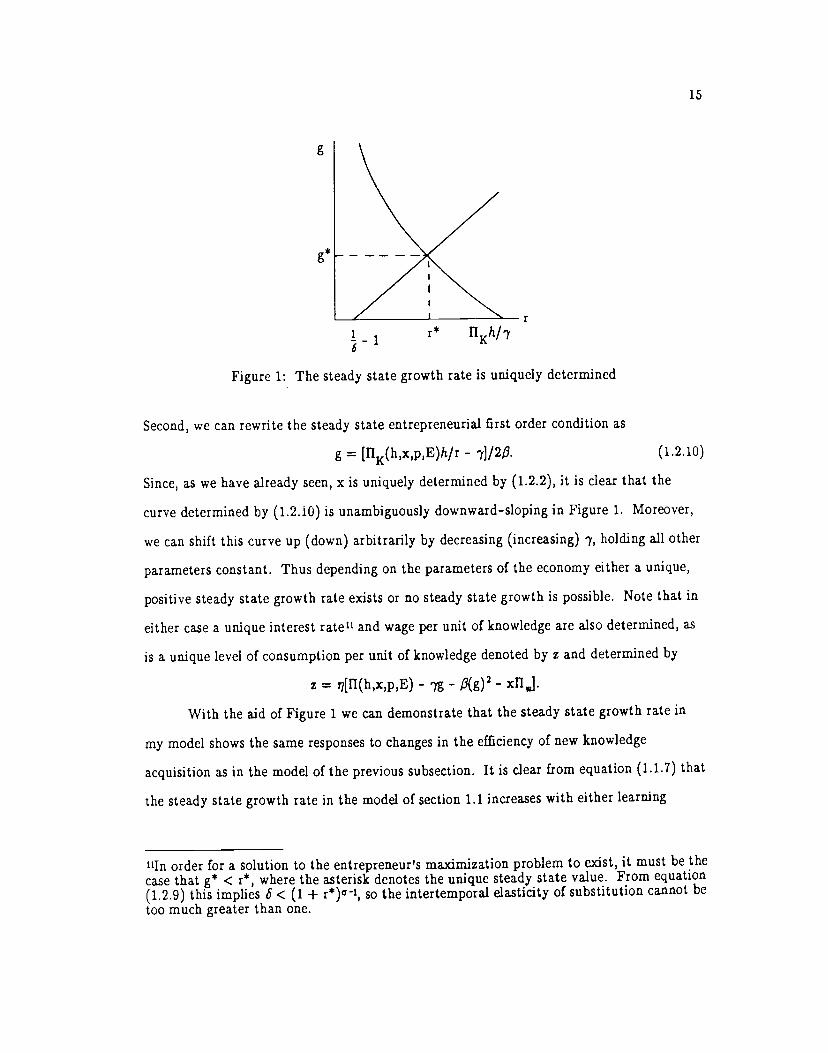
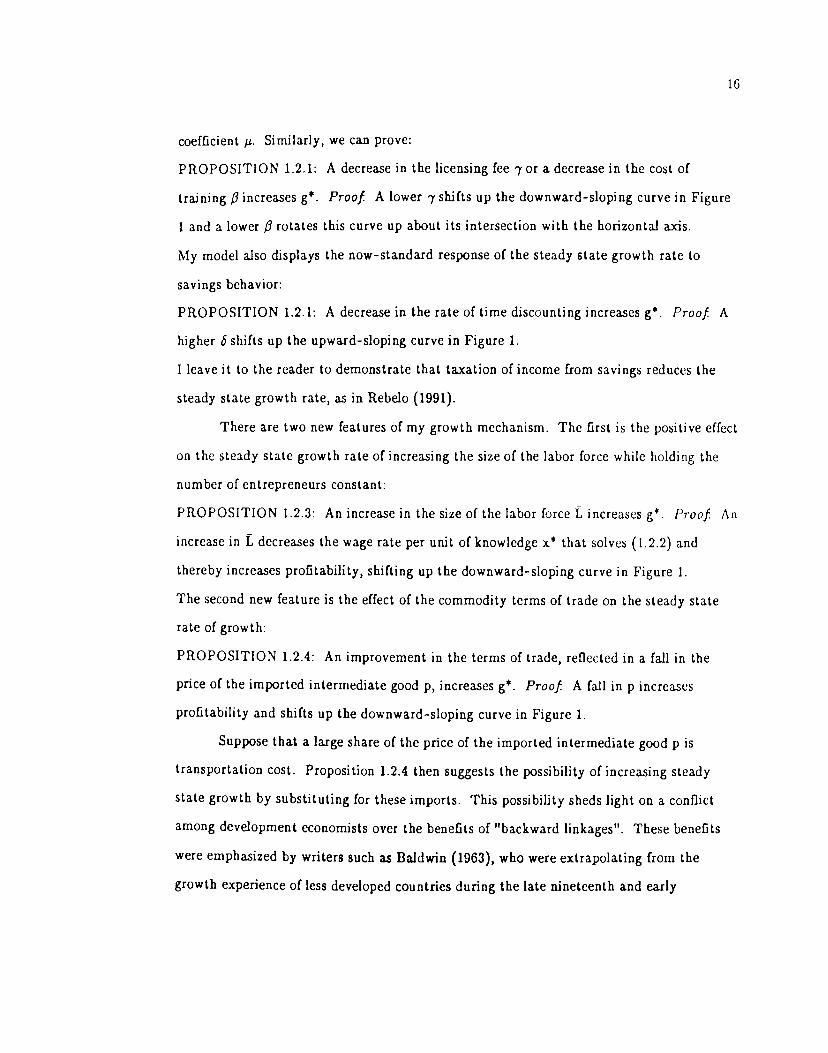
g = [5(1 + r)]" — 1. (1.2.9)

This equation determines an upward-sloping curve in r, g space. It is plotted for the case

= 1 in Figure 1.

15

g

g*

r

Figure 1: The steady state growth rate is uniquely determined

Second, we can rewrite the steady state entrepreneurial first order condition as

g = [flKO,x,p,E)h/r- y]/2fi. (1.2.10)

Since, as we have already seen, x is uniquely determined by (1.2.2), it is clear that the

curve determined by (1.2.10) is unambiguously downward-sloping in Figure 1. Moreover,

we can shift this curve up (down) arbitrarily by decreasing (increasing) y, holding all other

parameters constant. Thus depending on the parameters of the economy either a unique,

positive steady state growth rate exists or no steady state growth is possible. Note that in

either case a unique interest rate and wage per unit of knowledge are also determined, as

is a unique level of consumption per unit of knowledge denoted by z and determined by

z = i7[fl(h,x,p,E) - - /3(g)2 - xfl,J.

With the aid of Figure 1 we can demonstrate that the steady state growth rate in

my model shows the same responses to changes in the efficiency of new knowledge

acquisition as in the model of the previous subsection. It is clear from equation (1.1.7) that

the steady state growth rate in the model of section 1.1 increases with either learning

'In order for a solution to the entrepreneur's maximization problem to exist, it must be thecase that g* < r, where the asterisk denotes the unique steady state value. From equation(1.2.9) this implies S < (1 + r*)I, so the intertemporal elasticity of substitution cannot be

too much greater than one.

1 r* HKhII71

16

coefficient p. Similarly, we can prove:

PROPOSITION 1.2.1: A decrease in the licensing fee or a decrease in the cost of

training /3 increases gt. Proof A lower 7 shifts up the downward-sloping curve in Figure

1 and a lower /3 rotates this curve up about its intersection with the horizontal axis.

My model also displays the now-standard response of the steady state growth rate to

savings behavior:

PROPOSITION 1.2.1: A decrease in the rate of time discounting increases g. Proof A

higher S shifts up the upward-sloping curve in Figure 1.

I leave it to the reader to demonstrate that taxation of income from savings reduces the

steady state growth rate, as in Rebelo (1991).

There are two new features of my growth mechanism. The first is the positive effect

on the steady state growth rate of increasing the size of the labor force while holding the

number of entrepreneurs constant:

PROPOSITION 1.2.3: An increase in the size of the labor force L increases g. Proof An

increase in L decreases the wage rate per unit of knowledge x that solves (1.2.2) and

thereby increases profitability, shifting up the downward-sloping curve in Figure 1.

The second new feature is the effect of the commodity terms of trade on the steady state

rate of growth:

PROPOSITION 1.2.4: An improvement in the terms of trade, reflected in a fall in the

price of the imported intermediate good p, increases g*. Proof A fall in p increases

profitability and shifts up the downward-sloping curve in Figure 1.

Suppose that a large share of the price of the imported intermediate good p is

transportation cost. Proposition 1.2.4 then suggests the possibility of increasing steady

state growth by substituting for these imports. This possibility sheds light on a conflict

among development economists over the benefits of "backward linkages". These benefits

were emphasized by writers such as Baldwin (1963), who were extrapolating from the

growth experience of less developed countries during the late nineteenth and early

17

twentieth centuries when transportation costs (especially for raw materials) were much

higher than at present. Writing about Taiwan in the 1960s, on the other hand, Riedel

(1976) states) "it might be argued that Taiwan has been so successful precisely because its

industrial structure lacks backward linkages" (p. 320). Even in the high transportation

cost case, however, one must be careful before concluding that import substitution will

raise the steady state growth rate. Suppose that temporary protection were imposed in

order to establish a domestic intermediate goods sector, and that in true llirschmanian

fashion the demand for import substitutes thus created called forth its own supply of

entrepreneurs, leading to establishment of a balanced growth steady state at which all

domestic demand for intermediate good output is met at a price lower than the import

price inclusive of transportation costs. 12 This clearly "successful" case of import

substitution does not necessarily raise the steady state growth rate. The reason is that the

competing demand for labor thus established tends to raise the wage rate per unit of

knowledge. In the case where Q and F are Cobb-Douglas, it is easy to construct numerical

examples where establishment of backward linkages through successful import substitution

raises gt and numerical examples where the opposite occurs.

2. Tradeables as the engine of growth

I now introduce the second, "following" productive sector into my model. Its

output is not traded internationally, for example due to high transportation costs or to

government-imposed barriers to trade. For this reason the relative price or terms of trade

between its output and the output of the traded goods sector is determined endogenously.

Aside from the fact that its output is nontraded, the behavioral assumptions for the second

sector are the same as for the first. Two additional important assumptions concerning

intersectoral behavior mentioned in the introduction to this paper are necessary, however.

'2For a full investigation of the properties of this steady state see Rauch (1992).

18

First, the managerial talents of entrepreneurs are entirely sector-specific so that no

intersectoral mobility of entrepreneurs in response to differential rents is possible. Second,

stocks of knowledge are also entirely sector-specific, so that nospillovers of knowledge

between sectors take place. These assumptions lead naturally to identification of the two

sectors with agriculture and industry, but could also be suitable forapplication to two

regions, where not only geographic distance but also cultural and even linguistic differences

hamper intersectoral mobility of entrepreneurs and information.

2.1 Steady state growth

We saw in the previous section that reductions in the cost of knowledge acquisition(decreases in or fi) in the traded goods sector increased the steady-state growth rate ofthe economy. If in fact the traded goods sector "drives" regional growth, this should not be

true for the nontraded goods sector. Instead, decreases in these parameters fornontradeables should have only level effects, reducing the cost of nontraded goods toconsumers in the steady state.

Denote the traded and nontraded sectors by a superscript T and N, respectively. Inaddition to the growth rate, interest rate, and wage per unit of (sector T) knowledge, two

new variables must now be determined in the steady state: the terms of trade between the

nontraded and traded sectors p and the ratio ofknowledge stocks RT/IN k. The twoadditional equations are the optimal investment decision for sector N entrepreneurs and the

market clearing equation for sector N output.

To keep matters simple I drop the intermediate good from my model. In theabsence of these inputs, we write each sector's firm-level production function as

Qi = H(f(J,Ki)Fi(Ei,Li), j = T,N. (2.1.1)It is then easily shown that we obtain the profit functions JIT(HT,w) and IIN(pHN,w),

where the constant arguments E have been suppressed to save notation. We see that the

role played by the intersectoraj terms of trade is similar to the role played by the

international terms of trade in the one-sector model of section 1.2: there an increase in p

19

reduced profits in the traded goods sector, while here it increases profits in the nontraded

goods sector that is competing with the traded goods sector for scarce resources.

Since there are only two variable arguments in each of the profit functions, to avoid

confusion with the one-sector model I denote the derivatives with respect to each of these

arguments by n{ and fl, respectively. We can then write the labor market clearing

condition as

- ,TT(HTw) - ,7NnN(pHNw) = L

or - ,7Tfl'(hTx) - ,7Nfl(phN) = L, (2.1.2)

where x is the wage per unit of sector T knowledge.

Consumers can now choose to allocate their consumption expenditure to either T or

N output. We therefore change the consumer objective function in section 1.2 to

[U(cT,c)]1/(1-), > 0, 0 < 5< 1,to�t<a,

where U(c,c) is linear homogeneous. This linear homogeneity implies that the marginal

utilities aU/f and ôU/Oc are functions only of the ratio c'/cT, which in turn implies

from the first-order condition (OU/&)/(ôU/ôc'') =Pt that c/c'' is a function only of

the price ratio Pt• We can therefore write U(cT,c) = c'v(p), and the Euler equation for

consumption of the traded good becomes

(cT./c)° = [v(pt)/v(pt.j)Ja[(5U/acT+j)/( OU/ocT)]5(1 + r.j).Again we can aggregate this first-order condition without regard to distribution of wealth,

yielding a new version of equation (1.2.3):

(C'',jC'f)° = + r+). (2.1.3)

We can find the optimal investment policy for an entrepreneur in each sector

following the same procedure as in section 1.2. We obtain a new version of equation (1.2.6)

for each sector:

= (1 + rt,t)[7T + 2(9T/T)1T] - [7T + 2(flT/fC''.1)1T+J

fl+1h,1p+1 = (1 + rt+t)[7N + 2(/R)I] — [7N + 2(flN/41)J41]. (2.1.4)

20

Finally, we add the condition that the market for nontraded output must clear in

every period. We note that CN ,lNfl?HN and CT/CN = A(p), A' > 0. Balanced trade

yields CT = ,7T[QT - 7T1T - (fiT/T)(JT)2] - N[7NJN + (/3/1)(1N)1• We can combine

these three equations with the fact that QT 11T - wrI' H''HT to get the market

clearing equation

- 7T1T - (fiT/T)(1T)1 - N[7NJN + (flN/N)(jN)2J = A(p),I1HN.In the steady state p is constant so (2.1.3) reduces to (1.2.9), giving us the same

upward-sloping curve in Figure 1 as in the one-sector model. For the traded goods sector

(2.1.4) reduces to the equivalent of (1.2.10):

T T T Tg = [fl1(h ,x)h /r - y . (2.1.5)

In the one-sector model x was determined by the labor-market clearing equation (1.2.2)

alone. The labor-market clearing equation (2.1.2), however, involves the new variables p

and k. To solve for the steady state, therefore, we need the steady-state entrepreneurial

first-order condition for sector N, which we obtain from (2.1.4):

g = [flj(phN,kx)phN/r -7N1129N (2.1.6)

where we have used the fact that along a balanced growth path we have g = 1T1T =

1N1N We also need the market clearing equation for sector N output, which when we

divide both sides by RN can be written:

??TkEHT(hTX)hT - 7Tg - flTg2] - ,N[7Ng + flNg = A(p),fl(phN,kx)hN. (2.1.7)

Determination of the steady state is summarized in Table 1.

I would like to show that the latter four equations in Table 1 determine a

downward-sloping curve in Figure 1, thus demonstrating uniqueness of the steady state

growth rate g* in the same manner as in the one-sector model of the previous section. It

proves simpler to analyze whether an increase in g causes a decrease in r rather than vice

versa. In section A2 of the Appendix it is shown that the direct effect ofg on r through the

optimal investment decisions is indeed negative, under the sufficient but far fromnecessary

condition that A(p) - A'(p)p> 0. (This condition is satisfied, for example, if

21

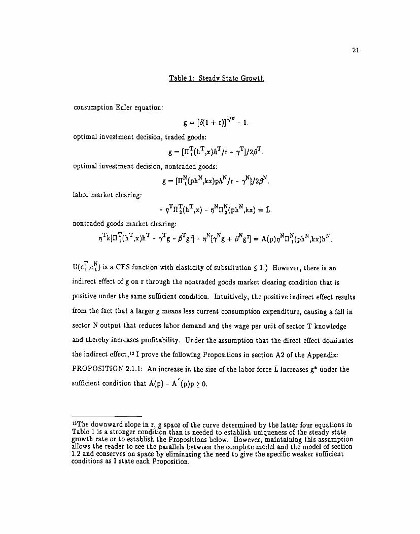
Table 1: Steady State Growth

consumption Euler equation:

g = [5(1 + r)J1 - 1.

optimal investment decision, traded goods:

g = [rI''(hT,x)hT/r 7T]/2T•

optimal investment decision, nontraded goods:

g = [ll(phN,kx)phN/rlabor market clearing:

- ,7TII'(hTx) - ,lNflN(phN) = L

nontraded goods market clearing:

Tk[flT(hTx)hT - - f3Tg - ,[71g + fiNg = A(p),rI(phN,kx)hN.

U(cT,c) is a CES function with elasticity of substitution 1.) However, there is an

indirect effect of g on r through the nontraded goods market clearing condition that is

positive under the same sufficient condition. Intuitively, the positive indirect effect results

from the fact that a larger g means less current consumption expenditure, causing a fall in

sector N output that reduces labor demand and the wage per unit of sector T knowledge

and thereby increases profitability. Under the assumption that the direct effect dominates

the indirect effect,'3 I prove the following Propositions in section A2 of the Appendix:

PROPOSITION 2.1.1: An increase in the size of the labor force L increases g* under the

sufficient condition that A(p) - A'(p)p � 0.

'3The downward slope in r, g space of the curve determined by the latter four equations inTable 1 is a stronger condition than is needed to establish uniqueness of the steady stategrowth rate or to establish the Propositions below. However, maintaining this assumptionallows the reader to see the parallels between the complete model and the model of section1.2 and conserves on space by eliminating the need to give the specific weaker sufficientconditions as I state each Proposition.

22

PROPOSITION 2.1.2: An increase in the cost of knowledge acquisition yT decreases g*

under the sufficient conditions that A(p) - A'(p)p � 0 and r � ghT/hT. Since restrictions

that imply r > g have already been assumed (see footnote 11), the latter condition is

satisfied if hT � hT, which holds if, for example, the function 11T is Cobb-Douglas.

PROPOSITION 2.1.3: An increase in the cost of training T decreases g* under the

suffident conditions that A(p) - A(p)p � 0 and r ghT/2hT.

Propositions 2.1.2-2.1.3 correspond to Proposition 1.1 in section 1.2, and are

consistent with the idea that the traded goods sector is the "engine of growth". The results

are different when we turn to sector N.

PROPOSITION 2.1.4: An increase in the cost of knowledge acquisition 7N increases g* if

U(c',c) is Cobb-Douglas. This effect approaches zero as approaches zero.

PROPOSITION 2.1.5: An increase in the cost of training decreases g* if U(c',c) is

Cobb-Douglas. This effect approaches zero as 1N approaches zero.

Propositions 2.1.4-2.1.5 show that changes in the cost of licensing knowledge for the

"lagging" sector perversely affect steady state growth, and changes in steady state growth

caused by either sector N knowledge acquisition parameter can be made arbitrarily small

by shrinking the size of the other parameter. We can see the underlying reason for this

property of my model by looking at Table 1 and observing that the only way in which

sector N can influence g* is by changing x*, the steady state wage per unit of sector T

knowledge.

Unlike their effects on steady state growth, the effects of the sector N knowledge

acquisition parameters on p should be robust. Consider a decrease in 7N or This

reduction in the cost of knowledge acquisition relative to sector T requires a decrease in the

profitability of knowledge acquisition relative to sector T in order to maintain balanced

growth, and this decrease in relative profitability is most directly accomplished by moving

the terms of trade against sector N. In order to do thecomparative static exercises needed

to verify this level effect intuition, I first need to establish that p is unique. Conditions

23

have already been given under which the balanced growth rate g* and interest rate r* are

unique. In section A2 of the Appendix I prove that pt, k*, and x are all uniquely

determined given g* and r* under the sufficient condition A(p) - A'(p)p 0. It is then

easy to also prove:

PROPOSITION 2.1.6: An increase in the cost of knowledge acquisition 7N (training)

increases p if U(c',c) is Cobb-Douglas and fiN (7N) equals zero.

Under the same conditions given for Proposition 2.1.6 it is easy to show that k* also

increases with rN or '4 The intuition is that the increase in or 13N temporarily

depresses knowledge growth in sector N, causing k* to rise until the increase in p restores

balanced growth.

2.2 Nontradeables: Pulled along or falling behind?

Since the model of section 2.1 yields exponential growth, we must normalize onone

of the knowledge stocks to obtain a stationary model whose stability we can analyze. In

the normalized model there is only one state variable, the knowledge stock ratio k, but two

control variables, the normalized investments of each sector. Unlike in the model of

section 1.1, a mathematically formal determination of whether my model is globally stable

given any set of parameters has not proved feasible. While it is in fact possible to obtain

some analytical results concerning local stability for certain special cases, it proves more

illuminating to combine an intuitive approach to the questions of interest with some

supporting simulations suggested by the model of section 1.1.

We saw in section 2.1 that, when g* and rt are uniquely determined under weaker

conditions so are the steady state knowledge stock ratio k* and the steady state terms of

trade p* Suppose that at some point in time k> k*. If the balanced growth path is

14Jf these conditions were eliminated while retaining the conditions for uniqueness, the effectof an increase in or fiN ()j p would be determined by the ratio of two 5 x 5determinants. The determinant in the denominator would be positive, while thedeterminant in the numerator would contain only one negative term, similar to the"indirect effect" above. This term would have to be dominated for the determinant to bepositive. Details are available from the author on request.

24

stable, sector T will "pull along" sector N by bidding up its terms of trade sufficiently

above p to cause it to acquire knowledge at a faster rate than does sector T. If the

balanced growth path is unstable, this terms of trade effect is too weak and sector N falls

further and further behind sector T in rate of knowledge acquisition, losing the competition

for labor and capital resources. The analogy to the model of section 1.1 is clear: there an

initial knowledge stock ratio greater than its balanced growth steady state value also yields

terms of trade for the lagging sector above their steady state value, which causes it to

acquire knowledge at a faster rate than the leading sector if the elasticity of substitution in

consumption is sufficiently small (less than unity).

This analogy suggests that the value of the elasticity of substitution in consumption

will be the key determinant of whether the balanced growth path in my model is stable. I

now try to see if this insight is borne out by simulations. In particular, I assign to

U(cT,cN) the CES functional form used in equation (1.1.3) above and consider what

happens to stability as I vary the elasticity of substitution c. Turning to the nontraded

goods market clearing equation in Table 1 above, it is easily shown that the function A(p)

associated with this CES specification is {[(1_Q)/0]}E• If 0 = .5 and the other parameters

of the model are such that p = 1, then one can see from Table 1 that it is possible to vary

without changing the balanced growth steady state. This is what I do in Figure 2, which

shows the results of simulations that all start with a knowledge stock ratio tenpercent

above the balanced growth steady state value but have different values of c. As expected,

the rate of convergence to the steady state declines with . For e > 3.5, the model becomes

locally unstable. Different initial percentage deriations of the knowledge stock ratio or

different underlying model parameters yield qualitatively similar results.

Analysis of why e >> 1 was required to generate instability in my model proves

helpful in understanding how the balanced growth process operates. In the model of

section 1.1 the variable affecting relative rates of knowledge acquisition is labor force

shares, while in my model it is relative profitability. Substituting K/K for p/p in the

25

last line of equation (1.1.5), we see that labor force shares are unaffected by a change in the

knowledge stock ratio if = 1, and move inversely (directly) with the knowledge stock

ratio if < 1 ( > 1), leading to stability (instability). In my model, however, one can

make a heuristic argument that relative profitability will be unaffected by a change in the

knowledge stock ratio only for some > 1. Suppose we disturb the steady state depicted in

Table 1 by a unanticipated ten percent increase in k. Holding g constant, this requires

adjustments in p and x to clear the nontraded goods and labor markets. Ignoring the term

N[yNg + fiNg in the nontraded goods market clearing equation, we can see that for c = 1

a ten percent increase in p and a constant x will dear both markets. Profitability of

investment in the traded goods sector is then unchanged, but we can see that profitability

of investment in the nontraded goods sector increases. Unchanged relative profitability

thus requires a percentage increase in p less than that in k, implying c > 1 in order to clear

the nontraded goods market. Inclusion of the term i[yNg + g2] only strengthens this

argument. Thus we see from Figure 2 that, as increases from unity towards its

"break-even" level, the percentage increase in p drops from about equal to about half the

percentage increase in k.

Figure 3 gives an example of the balanced growth process at work. It is suggested

by the experience of the Punjab cited in the introduction to this paper, where extension

services brought Green Revolution technology to the agricultural sector, stimulating its

growth which in turn stimulated industrial growth. An unanticipated fall in training costs

causes the rate of investment in the traded goods sector to accelerate above its previous

steady state level. The terms of trade for sector N are bid up, "pulling along" investment

there and allowing its rate of growth to catch up to that of sector T, thereby establishing a

new steady state at which growth in both sectors is permanently higher.

3. Liberalization and unbalanced growth, with an application to Chile

Suppose that sector N output is not traded internationally due to

26

government-imposed barriers to trade. We saw in the model of section 1.1 that

(generically) trade liberalization put the economy on a higher steady state growth path. I

begin this section by showing that the same is true in my model, and then go on to

simulate its transition dynamics (nonexistent in the model of section 1.1) and apply this

simulation to the Chilean economy after 1973.

I suppose that after liberalization the intersectoral terms of trade are fixed at p by

world markets. In section Al of the Appendix I prove that if a positive balanced growth

rate is feasible, then given any p" the balanced growth rate g**, interest rate r**, wage

per unit of sector T knowledge x1, and ratio of sector T to sector N knowledge k** are all

uniquely determined. In other words, for any p there exists a unique solution to the first

four equations in Table 1 (the market clearing equation for nontraded goods is no longer

relevant), provided g** > 0. As discussed in the introduction to this paper, in the absence

of the terms of trade adjustment mechanism this steady state should be globally unstable,

by which I mean that given any initial Ic k** the economy will diverge still further from

k**. A heuristic argument for this instability runs as follows. Suppose that at some point

in time Ic > k**. (The argument is symmetric if k < k**.) This "head start" for sector T

implies that the wage per unit of knowledge in sector T relative to sector N is lower than in

the steady state, making the profitability of investment in sector T relative to sector N

higher than in the steady state. Since the rate of knowledge acquisition in the two sectors

is equal in the steady state, knowledge growth in sector T is now relatively higher, causing

k to increase still further. An analytical proof that the balanced growth steady state is

globally unstable when the intersectoral terms of trade are fixed is given in Rauch (1992)

forthecasefiT=flo.Suppose that our country is on the balanced growth path of the model of section 2.1,

and then policy makers decide to remove the protection given sector N, causing the

27

domestic terms of trade to fall from p to the exogenously given world level p**.15 The

following Proposition is proven in section Al of the Appendix:

PROPOSITION 3.1: The balanced growth steady state knowledge stock ratio k** varies

directly with the exogenously given terms of trade

It follows from Proposition 3.1 that the knowledge stock ratio k* for the country prior to

liberalization will be above the k** associated with the post-liberalization terms of trade,

so after liberalization the country finds itself in a situation where sector T has more

knowledge relative to sector N than balanced growth would warrant. Following the

argument of the preceding paragraph, the country now embarks on an unbalanced growth

path where k increases without limit. Along this divergent path wages are rising since

investment in sector T is positive. Nevertheless since k is increasing we can see from the

labor-market clearing condition that x, the wage per unit of sector T knowledge, falls

steadily, increasing the profitability of knowledge acquisition in sector T and the share of

the labor force that it employs. Thus investment and production in the economy

ultimately become completely specialized in sector T.

I can now state

PROPOSITION 3.2: Liberalization raises the steady state growth rate. Proof We saw in

section 2. 1 that sector N only influences the steady state growth rate through its effect on

x, the wage rate per unit of sector T knowledge. Since its demand for labor in the labor

market clearing equation of Table 1 goes to zero in the new steady state, the value of x in

the new steady state is dearly less than x and thus the new steady state growth rate is

greater than g*.

The shift from the balanced growth steady state to a one sector steady state is in essence

equivalent to an increase in L in the model of section 1.2, and thus Proposition 3.2 actually

I5Jf p4 were below ptt the output of sector N would be exported, contradicting theassumption that its output is nontraded. In the knife-edge case pt = ptt the countryremains on the balanced growth path.

28

follows from Proposition 1.2.3.

Although the new steady state will be the same, the unbalanced growth path

following liberalization may be very different depending on the relative sizes of the two

sectors along the balanced growth path. Suppose, for example, that sector N was by far

the larger sector, perhaps by virtue of a much greater weight in consumer demand. Since

the two sectors were growing at the same proportionate rate, sector N was accounting for

the buJk of aggregate investment. When its entrepreneurs reduce or cease their knowledge

acquisition, the stimulus provided to investment in sector T by lower expected wages per

unit of sector T knowledge may not be sufficient (because of convex training costs) to

prevent a fall in the overall growth rate of the economy. Eventually, however, because

sector N is now shrinking relative to sector T, the accelerated growth of the latter must

dominate overall per capita income growth so that the unbalanced growth rate becomes

higher than the balanced growth rate. In sum, depending on the parameters of the

economy, "liberalization" may cause an immediate acceleration of growth, a brief growth

"recession", or a prolonged growth "depression" before the ultimate higher growth rate is

attained.

I shall argue below that it is useful to view the Chilean economy after l73 as being

on an unbalanced growth path following a liberalization, with agriculture and

manufacturing playing the roles of sectors T and N, respectively. I focus on Chile because

it is currently viewed by many policy makers from Latin America to Eastern Europe as a

model for economic restructuring. I stick to this case study rather than looking at

liberalization experiences more broadly because the Chilean trade liberalization was

atypically dear-cut. According to Edwards and Edwards (1987), "Between 1974 and 1979

Chile was transformed from a highly closed economy, where international transactions were

severely repressed, into an open economy whose foreign trade corresponded quite dosely to

the neoclassical ideal [p. 109]."

Since Chileans speak of the period 1974-1984 as a "lost decade" of economic growth,

29

it is interesting to explore whether liberalization is in fact capable of generating a

prolonged growth slowdown in my model starting from a balanced growth path that at

least superficially mimics the pre-liberalization Chilean economy. I thus choose simulation

parameters that yield a steady state balanced growth rate gt of two percent (roughly the

Chilean average for 1950-1973), a ratio of sector T to sector N output along the balanced

growth path of one-quarter (roughly equal to the ratio of agricultural to manufacturing

output in Chile in 1973), and a new steady state growth rate (in an economy specialized in

sector T) of 4 percent (close to the Chilean average for 1984—1991). To facilitate

simulation I adopt Cobb-Douglas functional forms for F and H and a CES functional

form with c = .5 for U. Parameters are chosen to make sector T production more

labor-intensive than sector N production in line with the realities of agricultural and

manufacturing production in Chile, but otherwise no additional attempts at verisimilitude

are made in choosing parameters. Two concessions are made to the solution powers of the

simulation program. 1) Agents are not allowed to anticipate the liberalization decision.

This permits us to treat the balanced growth knowledge stock ratio k* as a given initial

condition, which results from entrepreneurial decisions in the previous period that turned

out to be incorrect ex post. 2) The relative price of sector N output falls sufficiently to

make it optimal for sector N entrepreneurs to cease all knowledge acquisition immediately,

so that their investment is set to zero. In the simulation reported in Figure 4, p'4' is 18

percent lower than the balanced growth steady state value p*.

Figure 4 shows that the growth rate of GDP initially falls to one percent from the

balanced growth rate of two percent. Essentially, this result occurs because the fall in the

wage rate and interest rate due to decreased sector N labor and investment demand,

respectively, cause the sector T growth rate to jump immediately almost to its new steady

state level of four percent. Since the share of sector T in GDP immediately jumps from 20

percent to over 23 percent as a result of the relative price change alone (i.e., not counting

labor force reallocation), a one percent growth rate for total GDP follows. 15 years are

30

required for the growth rate to return to its balanced growth level of two percent.

While Figure 4 would appear to depict a "painIu.l" process of transition to a higher

steady state growth rate, in fact welfare as measured by Ej(.95)tlog(U) is higher at

every r with liberalization than without. The reason is that liberalization causes a fall in

the price of sector N output, which by assumption is the good on which consumers spend

most of their income.16 As Figure 5 shows, only after ten years has slower growth relative

to a hypothetical continuation of balanced growth dissipated the initial increase in U that

results from liberalization. The following discussion of the Chilean experience with

liberalization will suggest ways in which a more realistic unbalanced growth model could

capture the welfare losses that appear to have taken place during Chile's transition period.

Chile is a country rich in natural resources that experienced a long period of

primary-product export-led growth during the late nineteenth and early twentieth

centuries. The Great Depression led to a collapse in the world prices of primary products

and was a powerful stimulus to import-substituting industrialization in Chile and

throughout Latin America. After World War II Chile, like virtually all other Latin

American countries, adopted a policy of government-led import-substituting

industrialization. In particular this meant prohibitive trade barriers to manufactured

imports, though many other incentives for industrial investment were offered such as

subsidized credit. This policy led to the creation of a highly diversified but inefficient

manufacturing sector that could not compete in international markets. Per capita GDP

during the period 1950-1973 grew at an average annual rate of about 2 percent (see Figure

6), slightly higher or lower depending on the data source. In late 1973 a new regime came

to power and began a sweeping program of economic liberalization. After a sharp

contraction in 1975, a boom that carried per capita GDP to a new peak in 1981 was

followed by another sharp contraction in 1982-3. By 1984per capita GDP was essentially

'No tariff revenue was lost as a result of liberalization because the tariff is prohibitive alongthe balanced growth path by assumption.

31

back at its 1973 level (itself already down from the peak in 1971), hence the phrase "lost

decade" of economic growth. Since 1984, however, per capita GDP has grown at an

accelerating rate, with an annual average over the period 1984-1991 above four percent.

While most observers perceive the end of the boom after 1981 as caused by

avoidable macroeconomic mismanagement (Edwards and Edwards 1987 is typical), I want

to argue that the "lost decade" of economic growth was the natural outcome of a transition

from balanced growth to unbalanced growth, the latter being led by agriculture and

agro-processing industry. This larger picture was masked by the 1976-1981 boom, which

appears to have been the result of a speculative bubble in finance and urban real estate.17

The macroeconomic mismanagement story correctly captures the jagged ups and downs

shown in Figure 6 for per capita GDP during the period 1973-1984, but misses the

connection between the medium to long term growth performance of the economy and the

underlying structural transformation that began in 1973. It is partly the perception that

this transformation has "taken root" that leads observers to see the current boom, unlike

that during 1976-81, as sustainable.

In support of my reinterpretation of Chilean economic performance after 1973 I offer

the evidence of Figures 7, 8, and 9. These figures show, respectively, that after 1973 there

was: 1) a complete reversal of the historically declining trend in the ratio of agricultural to

manufacturing GDP; 2) an explosion of agricultural exports and manufacturing imports,

and 3) a rising import penetration ratio in manufacturing after one removes

agro-processing industries, much of the output of which would be classified as agricultural

if the Standard Industrial Trade Classification (SITC) was used. The trends predicted by

the unbalanced growth model, obscured by the 1981 peak in demand for manufactures

(both domestic and imported), are brought out by the estimated time trends included in

'7Morandé (1992) reports that an index of the real price of housing in Santiago more thanquadrupled from early 1976 to early 1981, then fell to its earlier level. Real stock pncesexperienced a similar boom and bust.

32

the Figures. Clearly, however, there are ways in which the data do not fit the stylized

story I am telling, which bring out several limitations in the ability of my simple model to

describe the real world. First, we note that during the period through 1973 that I identify

with balanced growth, Chile was a net importer of the products of agriculture, the sector I

identify with sector T. The true source of foreign exchange for the Chilean economy was

copper mining, not agriculture. The copper mining sector does not fit into the framework

of my model because wide swings in the world price of copper dominate any productivity

changes due to accumulation of knowledge and because its extremely low labor intensity

minimizes the importance of its labor market interactions with other sectors.18 Second, a

related point is that the ratio of agricultural to manufacturing production is in secular

decline through 1973, while of course this ratio should be constant along a balanced growth

path. This reflects not only government intervention on behalf of manufacturing over and

above protection, but also the operation of Engel's law as incomes rose while (as shown in

Figure 8) the Chilean agricultural and manufacturing sectors remained virtually closed to

international trade. Third, and most important, the model of unbalanced growth implies

that after liberalization the manufacturing sector will ultimately disappear completely.

The limitation of the model revealed by this undoubtedly false prediction flows from the

fact that all entrepreneurs/firms within a sector are identical, so if one ceases to invest and

ultimately goes out of business so must all the others.

One more key feature of the Chilean liberalization experience that is left out by my

market clearing model is the tremendous increase in unemployment that occurred: the

unemployment rate averaged 4.5 percent during the period 1966-1972 but never dropped

below 10 percent during the 1976-1981 "boom".19 This probably accounts for the fact that

'81n 1973 the ratios of mining employment to manufacturing employent and agriculturalemployment were 16.9 and 15.4 percent respectively (data supplied by Joseph Grunwaldfrom computations by Esteban Jadresic.t9The sources for the unemployment data are Economic and Social Indicators and variousissues of the Mont hl Bulletin of the Central Bank of Chile.

33

Chile did not merely experience a growth slowdown but an actual growth stoppage during

the period 1974-1984. This suggests that it is the assumption of costless movement of

labor between sectors that prevents my unbalanced growth model from capturing the

"painfulness" of the Chilean liberalization experience.

4. The effects of economic integration

Consider two countries or regions with separate labor markets. The two countries

or regions may be specialized in production of different goods which they trade with the

rest of the world (induding each other) at given world prices, or they may produce the

same good but be unable to exchange entrepreneurs and information due to geographic

distance or cultural and linguistic differences. Each country or region is on its own steady

state growth path as described by the model of section 1.2 (omitting the intermediate

good).

Now suppose the two countries or regions unite to become one country with free

internal labor mobility. If the new country adopts a policy of free trade, so that the

relative price of the regional outputs remains unchanged compared to the pre-integration

situation, then (as noted in the previous section) we know that there exists a unique

associated with this pt that yields balanced growth. (If the two regions produce the same

good then p is identically one, and if their knowledge acquisition technologies arc also the

same it is easily shown that k** equals one as well.) I also argued in section 3 that this

balanced growth steady state is globally unstable. Thus we expect that under free trade

one region will go into relative decline in the sense that its entrepreneurs will become

progressively poorer relative to those in the other region and will employ a monotonically

decreasing share of the new country's labor force. This implies continual emigration from

the declining region even in the case where the two regions produce different goods if

entrepreneurs in the booming region find that they need to continue to locate their

production there in order to benefit from knowledge spillovers in their industry.

34

Which region will ultimately dominate the integrated economy? To avoid

introducing new notation for the knowledge stock ratio and the terms of trade we label the

regions T and N. We can then say that region T (N) will dominate if the knowledge stock

ratio k at the time of integration is greater (less) than k**. It obviously follows that region

j is more likely to dominate the greater is at the time of integration. Since we already

saw in Proposition 3.1 that k** increases with p", a region is also more likely to dominate

the higher is the relative price of its output on world markets. Intuitively, a greater

knowledge stock or better terms of trade both act to raise the absolute wage rate of a

region, so that economic integration makes investment by that region's entrepreneurs more

profitable when it causes the new wage rate to settle in between the two old ones. By a

straightforward modification of the proof of Proposition 3.1 in the Appendix, the reader

can show that k** increases (decreases) with and T (N and jr), from which it can be

deduced that a region is more likely to dominate the easier is its acquisition of knowledge.

Again the intuition for this result runs through greater profitability of investment. While

the possible asymmetry between the production functions for the outputs of the two regions

prevents us from proving a Proposition, I have established a presumption that if, at the

time of economic integration, one region has a wage rate and growth rate greater than or

equal to those of the other region (with one strict inequality), that region's entrepreneurs

will ultimately employ the entire labor force of the integrated economy. It is easy to

construct examples where the region with the higher wage rate but lower growth rate or

vice versa will not dominate, simply by manipulating the ratio of the region's labor force

endowment to its entrepreneurial endowment. This ratio affects the absolute wage rate

and the growth rate in opposite directions, but it becomes irrelevant to relative

profitability after economic integration.

In the steady state the new country must grow faster than the region that came to

dominate the economy did in isolation: economic integration has simply provided this

region with a source of cheap labor, lowering the wage rate per unit of knowledge and

35

thereby increasing profitability and the growth rate. It is nevertheless theoretically

possible that this growth rate is lower than was the growth rate in isolation of the region

that declined. Let us set aside this case and suppose that in its steady state the new

country grows faster than did either of its component regions in isolation. Following the

analysis of liberalization in the previous section, immediately after economic integration

the new country may nevertheless grow slower than did either region in isolation if, for

example, the declining region was sufficiently larger than the booming region. Also as in

the case of liberalization, the welfare effect of any initial slower growth due to economic

integration may be more than offset by an initial efficiency gain, which now results from

the integration of two previously separate labor markets.

If it is the case that the two regions are specialized in producing different goods,

suppose that the quantity supplied of the output of the region that would decline under free

trade is smaller than the quantity demanded by the new country at the initial world price

ratio. It is then possible for a policy such as a common external tariff to allow the relative

price of that output to rise above the world price sufficiently to permit convergence to the

balanced growth path described in Table 1. How will the steady state growth rate compare

to the growth rates of the two regions in isolation? This is unclear since there need not be

any cheap labor effect: from the point of view of either region both labor supply and

competing labor demand are being added by economic integration. In fact, I have

constructed numerical examples where the new steady state growth rate is in between the

old regional growth rates, where it is above both old growth rates, and where it is below

both old growth rates. Of course we do know that the new country must grow slower along

the balanced growth path than it would have if it had been allowed to specialize in the

output of the region that would have dominated under free trade. It therefore appears that

in the choice between free trade, yielding an unbalanced growth path, and protection,

yielding a balanced growth path, the new country must trade off regional equity against

not only static but also dynamic efficiency.

36

It is interesting to view the much-studied problems of the South of Italy in light of

the discussion in this section. It is generally agreed that per capita output was lower in the

South than in the North of Italy when the country was unified in 1861. At that time the

tariffs between the various Italian states were eliminated and low Piedmontese external

tariffs were substituted for the much higher external tariffs of the Kingdom of the Two

Sicilies (the South). In line with the discussion above, let us think of the North and South

of Italy in 1861 as two regions that produce the same good but are unable to exchange

entrepreneurs and information. Given the initial difference in per capita output and the

closer proximity of the North to Northwest Europe, the source of the most advanced

technological knowledge at the time (effectively giving the North a superior knowledge

acquisition technology), it is reasonable to assume that the ratio of the Northern to

Southern knowledge stock exceeded k** at the time of Unification. My model then predicts

that a process of unbalanced growth should have begun, with continual migration of the

Southern labor force to the North and decline in Southern per capita income relative to the

North. These events did indeed take place, but there is considerable debate over their

timing. The censes of 1861, 1881, and 1901 show a faster rise in industrial employment in

the South than in the North up to 1881, followed by a sharp fall in Southern industrial

employment versus a continued increase in the North. King (1985, pp. 35-37) believes a

relative decline in Southern industrial employment began immediately but was masked by

a "rogue" census in 1881. Allen and MacLennan (1970, pp. 37-38) argue that the Southern

economy was relatively isolated until the mid—1880s, when the new State's program of

bringing the Southern road and railway network up to Northern standards began to bear

fruit, after which time the regional product and labor markets were more integrated and

the Southern decline began. But in any case, no significant decline in relative Southern

income was measured until after 1901, simply because neither region registered significant

per capita income growth before then. From 1901 to 1951, however, several different

statistical sources all support the occurrence of a more or less monotonic decline in relative

37

Southern income.20 According to Allen and MacLennan (1970,p. 40) virtually the entire

increase in Italy's agricultural output between 1900 and 1940 occurred in the North, and

industrial employment declined by about 10 percent between 1901 and 1936 in the South

but grew by roughly 50 percent in the North.

Since 1950, massive government transfers from the North to the South have allowed

the latter to keep pace with or even catch up slightly to the former in terms of per capita

GDP (OECD 1990, p. 70). Migration from the South to the North was nevertheless about

two million between 1951 and 1961 and again between 1961 and 1971, 600,000 between

1971 and 1981 and 100,000 between 1982 and 1988 (OECD 1990, p. 76, n. 38). The clear

slowdown in migration does not appear to reflect greater employment generation in the

South since the Southern unemployment rate rose to over 20 percent in 1988, more than

three times the level in the North (OECD 1990, p. 71). Modernization and growth has

definitely taken place in the South since 1950, but Northern entrepreneurs have been the

agents of this progress according to the literature surveyed by King (1987, pp. 19 1-192).

This indicates a gradual overcoming of the barriers of geographic distance, culture and

language that originally prevented the interregional mobility of entrepreneurs and

information, so that in terms of the discussion of this section the movement of the Italian

economy towards a steady state where Northern entrepreneurs employ the entire labor

force need not imply the emptying of the South in the long run.

5. Summary and conclusions: Application to the transition in Eastern Europe?

In this paper a mechanism of endogenous growth suitable for investigation of

sectoral or regional interaction was developed. It was shown how the high value placed on

production linkages by economic historians might be reconciled with the high value placed

on openness (often implying lack of linkages) by observers of contemporary less developed

20See the sources cited in OECD (1990, p. 64, n. 24) and Allen and MacLennan (1970, p. 39,n. 1).

38

countries. When the output of one sector is traded and the output of the other is

nontraded, it was shown how the traded goods sector acts as the "engine of growth" in the

sense that its profitability of knowledge acquisition primarily determines the steady state

aggregate growth rate. It was also shown how sectors or regions interact out of steady

state through product, labor, and capital markets, and in particular how if the former

interaction dominates the growth of one sector "pulls along" the growth of the other while

if the latter two interactions dominate one sector or region booms while the other declines.

The paper built on these results to show why liberalization of foreign trade should lead to a

transition from a lower to a higher steady state growth rate and why, during the course of

this transition, growth might initially be even slower than before liberalization. A final

application to economic integration of previously separate regions or countries showed that

the largest growth effects are to be had if one region is allowed to decline and provide a

source of cheap labor for the other region.

One way in which the theory developed in this paper could be profitably extended is

by developing the spatial implications of the balanced growth model in the case where

transportation costs cause the output of sector N to be nontraded. The spatial boundary of

tradeability could be determined endogenously, thereby defining a region within the

country. If this region is growing faster than the rest of the country a spatial

agglomeration at the regional level could result that is reminiscent of that described by

Krugman (1991) but is driven by a leading, technologically progressive industry as in

Perroux (1955).

A more speculative extension of the theory developed in this paper would be

application of the unbalanced growth model to the transition from state socialism to

capitalism. McMillan and Naughton (1992) argue that the immediate acceleration of

growth that followed reform in China compared to the depression that accompanied the

transition in much of Eastern Europe indicates the advantage of "evolutionary" over

"big-bang" reform. They point to three key factors in China's reform success (p. 131):

39

"first, massive entry of non-state firms; second, a dramatic increase in competition, both

among state firms and between state firms and non-state firms; and, third, improvements

in the performance of state-owned firms resulting from state-imposed market-like

incentives." Let us interpret sectors T and N in section 3 above as the non-state sector

and state enterprise sector, respectively. Entrepreneurs in the non—state sector acquire

knowledge in order to better meet the needs of the market while "entrepreneurs"

(manager-bureaucrats) in the state sector acquire knowledge in order to better meet the

needs of the state plan. In a "big-bang" liberalization further acquisition of the latter type

of knowledge is useless and the incumbent managers of state enterprises are unqualified to

acquire the former type of knowledge, hence investment on the part of state enterprises

dries up. Since the state sector is by far the larger sector initially, growth plummets and

could even turn negative if we allowed for costly movement of labor between the state and

non-state sectors. With an evolutionary liberalization of the type undertaken by China, on

the other hand, the state plan is gradually adjusted to become more "market-like" and

state enterprise managers either learn how to respond to the new incentives or are replaced

by people who are able to learn how, and in the limit they are not at a disadvantage

relative to non-state sector entrepreneurs with regard to further knowledge acquisition and

investment. State enterprises and non-state enterprises can then be viewed simply as firms

of different size within a unified economy, and there is no reason for investment to collapse

in either "sector". In short, the evolutionary reform policies followed by China work to

maintain investment by state enterprises, which is necessary to avoid a transitional

depression because the state sector is initially so much larger than the non-state sector.

40

APPENDIX

AO. Assumptions on second derivatives of the profit functions derived in section 2

Throughout this Appendix we will need assumptions on the second derivatives of

our profit functions that are stronger than the restrictions implied by the convexity

property we get from standard microeconomic theory. For example, convexity tells us that

the second derivative with respect to the price of output is nonnegative, so that output

supply functions are not downward-sloping, but we need to assume that output supply

functions are strictly upward-sloping, implying that this second derivative is positive. All

of the assumptions made here are satisfied if, for example, the underlying production

functions are Cobb-Douglas, as they are in all of the simulations conducted in the text.

ASSUMPTION AO.1: flJ1> 0, j = T,N.

This is true if and only if the supply functions are upward-sloping.

ASSUMPTION A0.2: fl2> 0, j = T,N.

This is true if and only if the input demand functions are downward-sloping.

ASSUMPTION AO.3: [P12 (= fl) <0, j = T,N.

This is true if and only if a marginal increase in knowledge increases input demand, or

equivalently if and only if an increase in input price reduces the marginal profit from an

additional unit of knowledge.

Al. Uniqueness and comparative statics with exogenous teruis of trade

Proof of uniqueness. I first demonstrate uniqueness of g** and r** by showing that

Figure 1 applies, i.e., that the two entrepreneurial first-order conditions and the

labor-market clearing condition yield g varying inversely with r. We totally differentiate

the appropriate equations from Table 1 to obtain

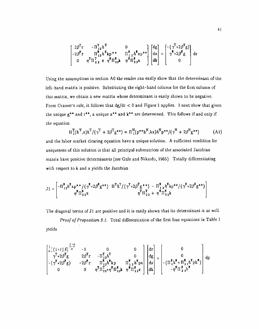
41

2;3T _fl'l2hT dg _(7T+2fiTg)

2flXr rI7hkp** I13hKxp** dx = yN+2flJg dr0 77TT 2 + ,7flk ,lMflx dk 0

Using the assumptions in section A0 the reader can easily show that the determinant of the

left-hand matrix is positive. Substituting the right-hand column for the first column of

this matrix, we obtain a new matrix whose determinant is easily shown to be negative.

From Cramer's rule, it follows that dg/dr < 0 and Figure 1 applies. I next show that given

the unique g** and rt, a unique and k** are determined. This follows if and only if

the equation

fl''(hT,x)hT/(7T + 2/3Tg**) = ll(p**hN,kx)hNp**/(7N + 2/?g**) (Al)

and the labor market clearing equation have a unique solution. A sufficient condition for

uniqueness of this solution is that all principal submatrices of the associated Jacobian

matrix have positive determinants (see Gale and Nikaido, 1965). Totally differentiating

with respect to k and x yields the Jacobian

Ji = _fl2hNxp*/(yN÷2Ig**) UThT/(7T+2IJTg**) - jj1 2hNkp**/(7N+2flNg**)ii fl22x 77 '22 + 77 [122k

The diagonal terms of Ji are positive and it is easily shown that its determinant is as well.

Proofof Propos1tion 3.1. Total differentiation of the first four equations in Table 1

yields

I -a

{(1÷r)61a -l 0 0 dr 0

7T2Tg 2Tr fl2hT 0 dg = 0dp

_(lM+2:3Ng) -2?r fl2hNkp [II2hKpx dx _(flhN+fl1h?Phro)

0 0 77TnT+77Kflk i7fl2x dk _17N[J 1hN

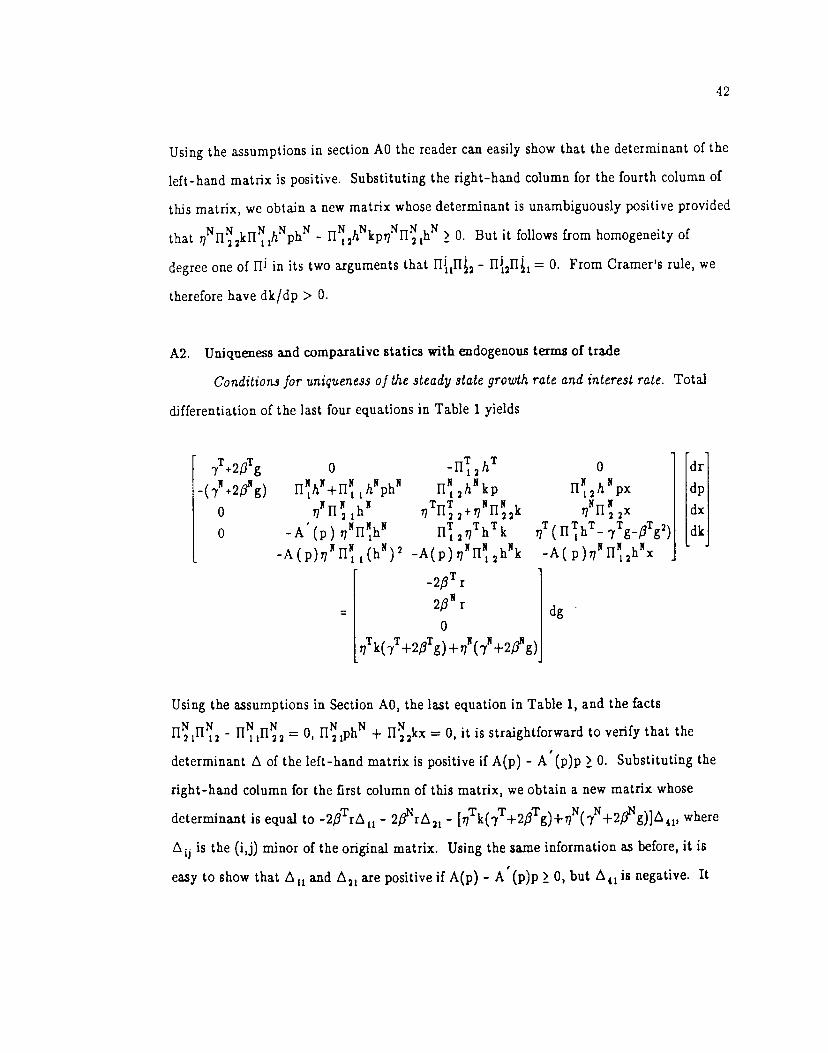
42

Using the assumptions in section AO the reader can easily show that the determinant of the

left-hand matrix is positive. Substituting the right-hand column for the fourth column of

this matrix, we obtain a new matrix whose determinant is unambiguously positive provided

that n2kfl1hNphN - fl2hNkpifI1hN � 0. But it follows from homogeneity of

degree one of fli in its two arguments that 11lt'12 - = 0. From Cramer's rule, we

therefore have dk/dp > 0.

A2. Uniqueness and comparative statics with endogenous terms of trade

Conditions for uniqueness of the steady state growth rate and interest rate. Total

differentiation of the last four equations in Table 1 yields

T T T T7+2/3g 0 -fl12h 0 dr

_(7N÷2flNg) flhN+U1hNphN rI2hNkp ll2hNpx dpNN N TT NN NN

o f121h 17 [122+17 1122k i fl22x dx

o _A(p),flhN .2?7ThTk ,lT(nhT_7Tg_fiTg2) dk_A(p),fl1(hN)2 _A(p),I1.2hNk -A(p)ifl2hx

2fiT

dg

Using the assumptions in Section A0, the last equation in Table 1, and the facts

[1211112 - = 0, fl1phN + flkx = 0, it is straightforward to verify that the

determinant i of the left-hand matrix is positive if A(p) - A'(p)p> 0. Substituting the

right-hand column for the first column of this matrix, we obtain a new matrix whose

determinant is equal to _2fiTr1j - 2LINrA21 where

is the (i,j) minor of the original matrix. Using the same information as before, it is

easy to show that H and 21 are positive if A(p) - A'(p)p> 0, but is negative. It

43

follows that the direct effect of g on r through the optimal investment decision, equal to

(_23Trii - 2/1Nr2i)/& is negative, arid that the indirect effect of g on r through the

nontraded goods market clearing condition, equal to

_[17Tk(7T+2flTg)+17N(7N+2flNg)]4j, is positive. If the direct effect dominates the

indirect effect, an increase in g will cause a decrease in r, and the latter four equations in

Table 1 determine a downward-sloping curve in Figure 1, proving the uniqueness of the

steady state growth rate and interest rate.

Proofs of Propositions 2.1.1-2.1.5: I again totally differentiate the last four

equations in Table 1 to obtain

o

_2fiNr rI2hNpx0 171122X

_17Tk(7T+2flTg) 17T(HhT 7Tg_fiTg2)

_iN(.2flNg) -A( p),fl2hNxdL

TddfiT

Nd7

d?

The assumption that the direct effect dominates the indirect effect of g on r implies that

the determinant of the left-hand matrix is positive. Therefore, to prove Propositions

2.1.1-2.1.5 all we need to do is substitute the appropriate column of the right-hand matrix

for the first column of the left-hand matrix and examine the sign of the determinant of the

new matrix.

Proposition 2.1.1: Substituting the first column of the right-hand matrix, the determinant

of the new matrix is -Afl, where is the (i,j) minor of the original left-hand matrix.

Simple algebra shows that -iis positive if A(p) - A'(p)p � 0.

0 11T ,T1 2

N K N

flhN+I1thNph 1112h kpNN N TryT N

17 1121h '7 U22+17 ll2k

-A(p) '7NflNhN

_A(p)'7JrI1(hN)2 _A(p)'7Nn2hNk

F o -r -2rg 0 0 1

_I0 0 0 r 2rgfI_i 0 0 0 0 I

N N 2'{ 0 '7Tkg '7Tk(g)2 g (gj

j

dg

dpdx

dk

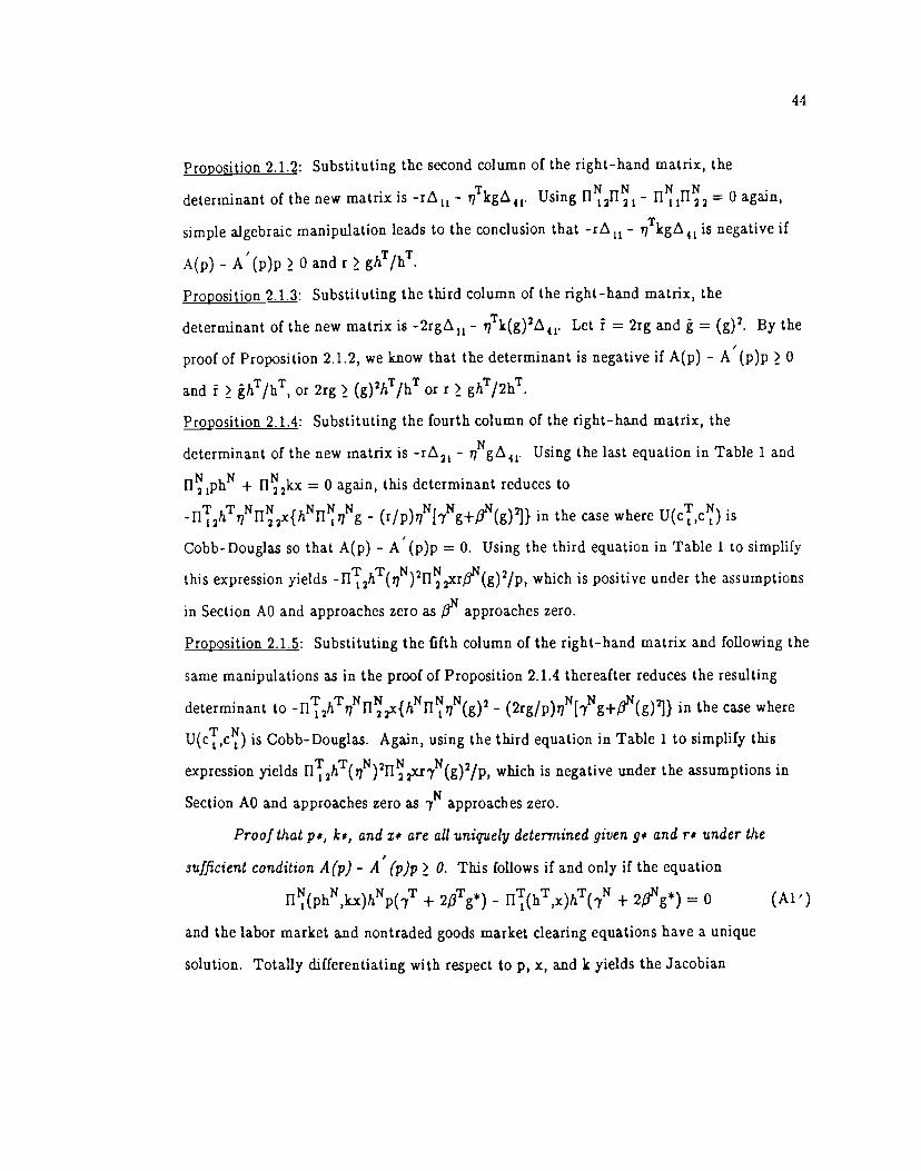
44

Proposition 2.1.2: Substituting the second column of the right-hand matrix, the

determinant of the new matrix is -r11 - iTkg41, Using fl2fl1 - I11I12 = 0 again,

simple algebraic manipulation leads to the conclusion that -r11 - llTkg4i is negative if

A(p) - A(p)p � 0 and r � ghT/hT.

Proposition 2.1.3: Substituting the third column of the right-hand matrix, the

determinant of the new matrix is -2rgL11 - ,lTk(g)24i Let = 2rg and = (g)2. By the

proof of Proposition 2.1.2, we know that the determinant is negative if A(p) - A'(p)p � 0

and ? � hT/hT, or 2rg � (g)2hTIhT or r � ghT/2hT.

Proposition 2.1.4: Substituting the fourth column of the right-hand matrix, the

determinant of the new matrix is -th21 - igi41. Using the last equation in Table 1 and

fl1phN + fl2kx = 0 again, this determinant reduces to

- (r/p) [yNg+(g)} in the case where U(c'',c') is

Cobb-Douglas so that A(p) - A(p)p = 0. Using the third equation in Table ito simplify

this expression yields _fl2hT(1N)2flxrfiN(g)2/p, which is positive under the assumptions

in Section A0 and approaches zero as fiN approaches zero.

Proposition 2.1.5: Substituting the fifth column of the right-hand matrix and following the

same manipulations as in the proof of Proposition 2.1.4 thereafter reduces the resulting

determinant to _fl2hTfl x{hNlll(g)2 - in the case where

U(ci',c) is Cobb-Douglas. Again, using the third equation in Table 1 to simplify this

expression yields fl2hT()2flxr7N(g)2/p, which is negative under the assumptions in

Section A0 and approaches zero as yN approaches zero.

Proof that p. k*, and z* are all tzniqizely determined given g and r# lhnder the

sufficient condition A(p) - A' (p)p � 0. This follows if and only if the equation

fl(phN,kx)hNp(7T + 2fiTg*) - rI'(hT,x)hT(lN + 2?g*) = 0 (Al')

and the labor market and nontraded goods market clearing equations have a unique

solution. Totally differentiating with respect to p, x, and k yields the Jacobian

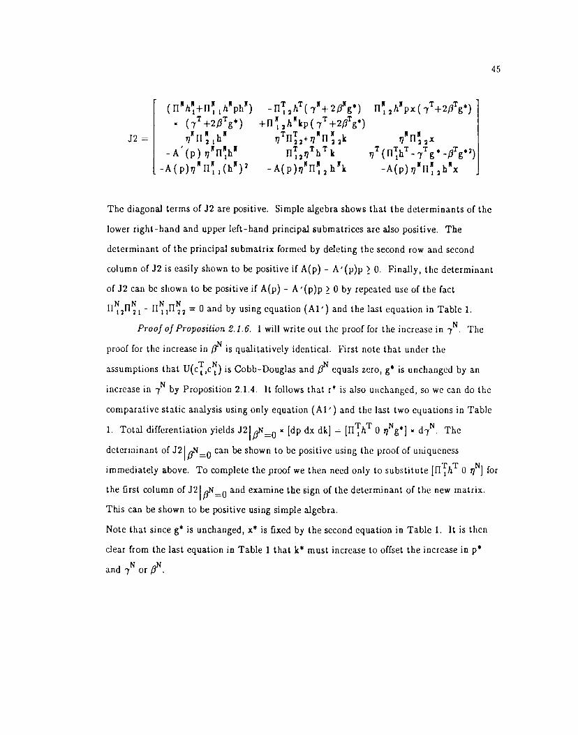
45

(IlNhN+lIJ 1hph) _fl2hT(7J2g*) fI 2hpx(,yT+2fiTg*)(7T+2flTg*) +112hJkp(7T+2/9Tg*)

N N N TT It It NJJ2= 17 fl21h 77 1122+17 fl22k 77 fl22x

-A(p)77flh 11T77ThTk 17T(nhT_7Tg*_flTg*2)-A(p)ifl 1(hK)2 -A(p),l1 2 hk -A(p)ifl 2h

The diagonal terms of J2 are positive. Simple algebra shows that the determinants of the

lower right-hand and upper left-hand principal submatrices are also positive. The

determinant of the principal submatrix formed by deleting the second row and second

column of J2 is easily shown to be positive if A(p) - A'(p)p � 0. Finally, the determinant

of J2 can be shown to be positive if A(p) - A'(p)p � 0 by repeated use of the factN N N N ." - 1''22 = 0 and by using equation (Al') and the last equation in Table 1.

Proof of Proposition 2.1.6. I will write out the proof for the increase in . The

proof for the increase in fiN is qualitatively identical. First note that under the

assumptions that U(cT,c) is Cobb-Douglas and fiN equals zero, g is unchanged by an

increase in 7N by Proposition 2.1.4. It follows that r* is also unchanged so we can do the

comparative static analysis using only equation (Al') and the last two equations in Table

1. Total differentiation yields J21flNQ [dp dx dk} = [nT/iT o 17Ng*J dyN. The

determinant of J2 fiN0 can be shown to be positive using the proof of uniqueness

immediately above. To complete the proof we then need only to substitute [U 'hT 0 ,jfor

the first column of J2N and examine the sign of the determinant of the new matrix.

This can be shown to be positive using simple algebra.

Note that since g* is unchanged, x is fixed by the second equation in Table 1. It is then

clear from the last equation in Table 1 that k* must increase to offset the increase in p'

and or

46

References

Ahiuwalia, Isher Judge, and C. Rangarajan. "A Study of Linkages between Agricultureand Industry: the Indian Experience." In The Balance Between In4ustry andAgriculture in Economic Development, Proceedings of the Eighth World Congress ofthe International Economic Association, Delhi, India, 1986. New York: St.Martin's, 1988.

Allen, Kevin, and M. C. MacLennan. Regional Problems and Policies in Italy and France.London: George Allen and Unwin, 1970.

Anderson, Dennis, and Panda Khambata. "Small Enterprises and Development Policy inthe Philippines: A Case Study." World Bank Staff Working Paper No. 468, 1981.

Baldwin, Robert E. "Export Technology and Development from a Subsistence Level."Economic Journal 73 (March 1963): 80-92.

Baer, Werner. The Brazilian Economy: Growth and Development. New York: Praeger,1989.

Chadha, G. K. The State and Rural Economic Tran.sforrnation: The Case of Punjab1950-1985. New Delhi: Sage Publications, 1986.

Child, Frank C., and Hiromitsu Kaneda. "Links to the Green Revolution: A Study ofSmall-Scale, Agriculturally Related Industry in the Pakistan Punjab." EconomicDevelopment and Cultural Change (January 1975): 249-275.

Edwards, Sebastian. "Trade Orientation, Distortions, and Growth in DevelopingCountries." Journal of Development Economics 39 (July 1992): 31-57.

Edwards, Sebastian, and Alejandra Cox Edwards. Monetarism and Liberalization: theChilean Ezperiment. Cambridge: Ballinger, 1987.

Gale, David and Hukukane Nikaido. "The Jacobian Matrix and Global Univalence ofMappings." Mathematische Annalen 159 (1965): 81-93.

Grossman, Gene, and Elhanan Helpman. "Hysteresis in the Trade Pattern." NBERWorking Paper No. 3526, December 1990.

Grossman, Gene, and Elhanan Helpman. Innovation and Growth in the Global Economy.Cambridge: MIT Press, 1991.

Hirschman, Albert. The Strategy of Economic Development. New Haven: YaleUniversity Press, 1958.

King, Russell. The Industrial Geography of Italy. New York: St. Martin's, 1985.

King, Russell. Italy. London: Harper and Row, 1987.

47

Krugman, Paul R. Geography and Trade. Cambridge: MIT Press, 1991.

Lucas, Robert E. "On the Mechanics of Economic Development." Journal of Monetan,,Economics 22 (July 1988): 3-42.

McMillan, John, and Barry Naughton. "How to Reform a Planned Economy: Lessonsfrom China." Oxford Review of Economic Polictj 8 (Spring 1992): 130-143.

Matsuyama, Kiminori. "Agricultural Productivity, Comparative Advantage, andEconomic Growth." Northwestern Discussion Paper No. 934, May 1991.

Morandé, Felipe. "The Dynamics of Real Asset Prices, the Real Exchange Rate, TradeReforms, and Foreign Capital Inflows: Chile, 1976-1989." Journal of DevelopmentEconomics 39 (July 1992): 111—139.

Murphy, Kevin M., Andrei Shleifer, and Robert Vishny. "Income Distribution, MarketSize, and Industrialization." Quarterly Journal of Economics 104 (August 1989):537-564.

Nicholls, William M. "Industrial-Urban Development as a Dynamic Force inTransforming Brazilian Agriculture, 1940-1950." In Erik Thorbecke, ed., The Roleof Agriculture in Economic Development. New York: National Bureau of EconomicResearch, 1969.

Nishimizu, Mieko, and John M. Page, Jr. "Productivity Change and Growth in Industryand Agriculture: An International Comparison." In The Balance Between Industryand Agriculture in Economic Development, Proceedings of the Eighth WorldCongress of the International Economic Association, Delhi, India, 1986. New York:St. Martin's, 1988.

OECD. OECD Economic Surveys: Italy. Paris: OECD, 1990.

Pack, Howard, and Larry E. Westphal. "Industrial Strategy and Technological Change:Theory versus Reality." Journal of Development Economics 22 (June 1986):87- 128.

Perroux, François. "Note sur la Notion de 'Pale de Croissance'." Economie Appliquée(January-June 1955): 307-320.

Ranis, Gustav, and John C. H. Fei. "A Theory of Economic Development." AmericanEconomic Review 51 (September 1961): 533-565.

Rauch, James E. "Balanced and Unbalanced Growth." University of California, SanDiego Discussion Paper 92—28 (August 1992).

Rebelo, Sergio. "Long-Run Policy Analysis and Long-Run Growth." Journal of PoliticalEconomy 99 (June 1991): 500-521.

Resnick, Stephen. "The Decline of Rural Industry Under Export Expansion: AComparison among Burma, Philippines, and Thailand, 1870-1938." Journal ofEconomic History 30 (March 1970): 51-73.

48

Riedel, James. "A Balanced Growth Version of the Linkage Hypothesis: Comment."Quarterly Journal of Economics 90 (May 1976): 319-322.

Romer, Paul M. "Crazy Explanations for the Productivity Slowdown." NBERMacroeconomics Annual 1987: 163-202.

_______________ 1989. "Capital Accumulation in the Theory of Long Run Growth."In Robert J. Barro, ed., Modern Bu-siness Cycle Theory. Cambridge: HarvardUniversity Press, 1989.

Stewart, Frances and Ejaz Gbani. "How Significant are Externalities for Development?"World Development 19 (June 1991): 569-594.

Tang, Anthony. Economic Development in the Southern Piedmont. Chapel Hill:University of North Carolina, 1958.

Teece, David J. The Multinational Corporation and the Resource Cost of TechnologyTransfer. Cambridge, MA: Ballinger, 1976.

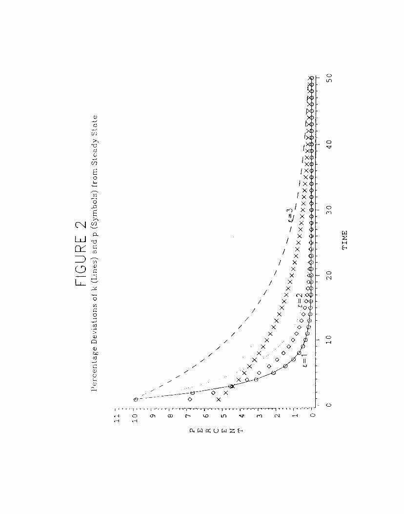
C)Lfl

p)

I>>

> I>.

IXXiX

U) IX

o X¾

XIX

0 f)'X -IXX

/ XI I-I

/ X )

XI XX i/ 'V(N/ X <)

X C'/ X (N.O0 / X Uo/ X O(

o X O)/ X/ x/ x ob/ X opQ) / X 0

-. — ______—t, 0 X0 X __ --C)

-.---'- -, ' T I

r1 CD O' CX) N -O 1(1 'J (N r4 C)

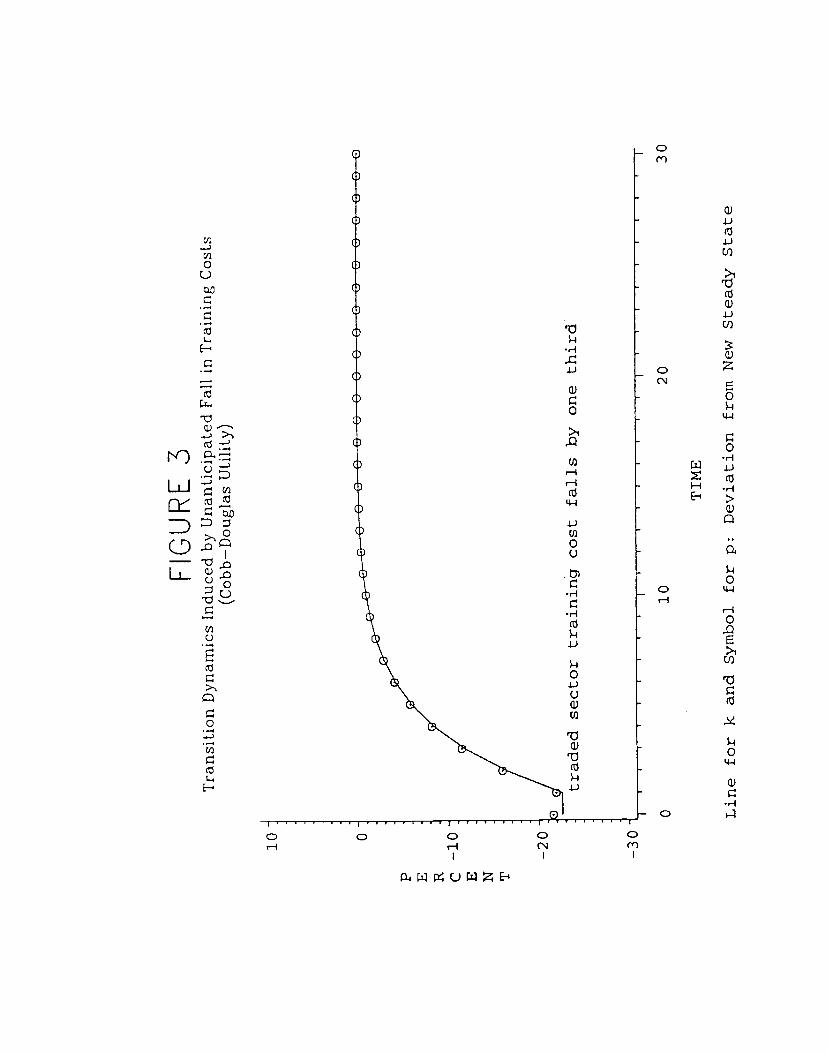
FIG

UR

E

3 T

rans

ition

Dyn

amic

s Ind

uced

by

Una

ntic

ipat

ed F

all

in T

rain

ing

Cos

ts

(Cob

b—D

ougl

as U

tility

)

10 0

p E

R

C -10

E

N

T

—20

trad

ed sector training cost falls by one third

—

1-1

I I

I I

I I

I I

I I

I

0 10

20

30

TIM

E

Lin

e fo

r k

and

Sym

bol

for

p:

Dev

iatio

n fr

om N

ew St

eady

Sta

te

3.0

2.9

2.8W

2.7

2.6

G 2.

5 R

2.

4 0

2.3

W 2.

2 T

2.1

H 2.0

1.9

1.8

1.7

1.6

1.5

1.4

1.3

1.2

1.1

1.0

FIG

UR

E

4 S

imul

ated

Gro

wth

Rat

es in

Per

cent

age

Ter

ms

unbala

R

A

T E

balanced

0 I

I I

I

I

I

I

I

I

I

-T

10

20

TIME

30

U

R

A

T I 0 1.

01

l.00

0.99

0.98

0. 9

7.

FIG

UR

E 5

Sim

ulat

ed W

elfa

re C

ompa

riso

n

1.09

1.08

1 . 0

7'

1.06

1.05'

1 . 04

1. 0

3'

1.02

(U unbalariced)/(U balanced)

0 10

1 1

T

I I

I I

I I

I I

I I

1111

11

20

30

TIM

E

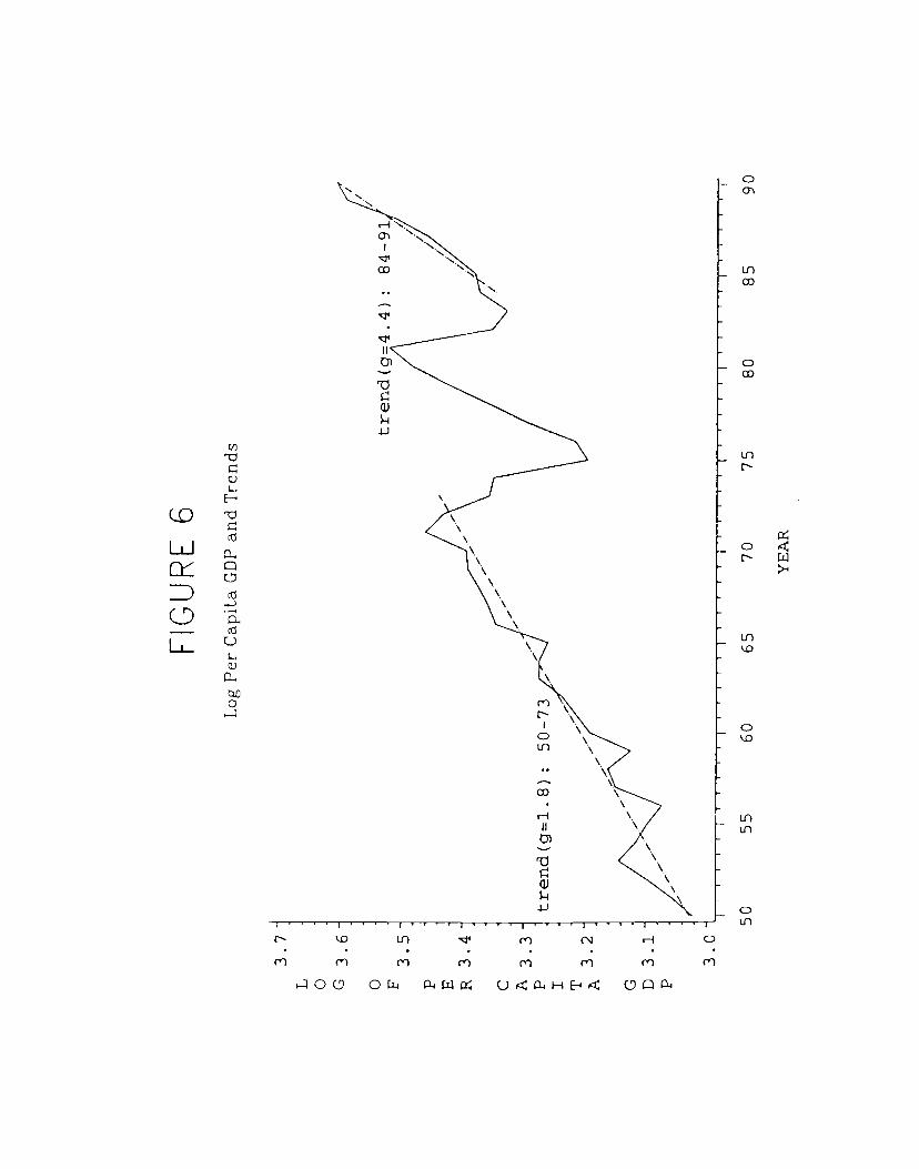
FIG

UR

E

6

Log

Per

Cap

ita G

DP

and

Tre

nds

L

0

G 0 F p E

R

C

A p I T

A

G

D p

3.7

3.6

3.5

3.4

3.3.

3.2

3.1

3.0-

trend

.4):

tren

d(g=

1.8)

: 50

-73

I j

I I

I I

I I

50

55

60

65

70

75

80

YE

AR

85

90

FIG

UR

E

7

Rat

io o

f A

gric

ultu

ral t

o M

anuf

actu

ring

GD

P

0.49

0.

48

0.47

0.

46

0.45

0.

44

0.43

0 .

42

0.41

R 0.40

A 0.39

T 0.38

0.37

o

0.36

0.35

0.34

0.33

0.32

0.31

0.30

0.29

0.28

0.27 -

0.26

60

65

80

85

90

YE

AR

trend: 73-91

trend: 60-72

I I

I

70

75

FIG

UR

E 8

Net

. E

xpor

ts o

f A

gric

ultu

re a

nd M

anuf

actu

res

3000

M

2000

L

L

I 0 N

0

—]0

00

—20

00

—30

00

S —4000

—5000

60

65

70

75

80

85

90

YE

AR

agricu.

trend: 73

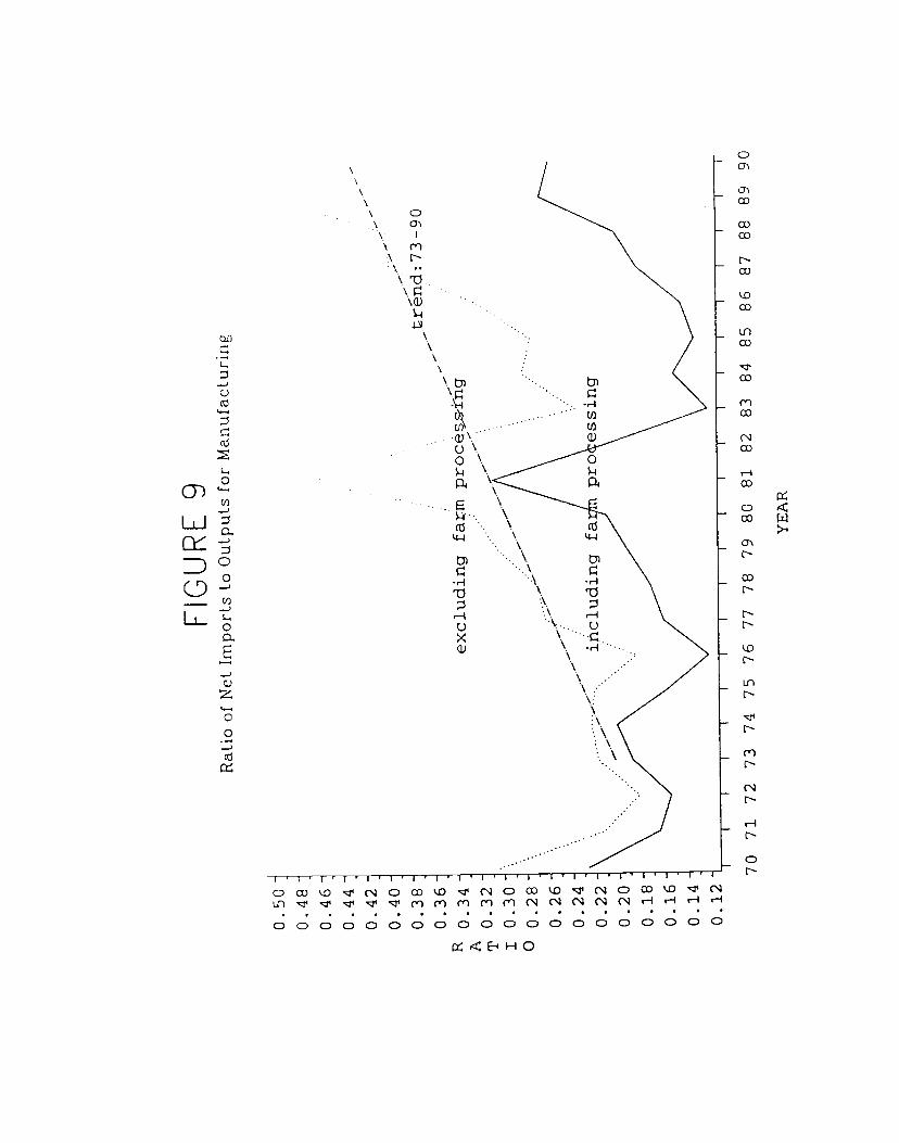
0.50

-

0.48

0.

46

0.44

0.42

0.40 -

0.38

0.36

R 034

0.32

I 0.30

0

0.28

0.

26

0.24

0.22

0.20

0.18

0.16

0.14'

0.12

FIG

UR

E

9 R

atio

of

Net

Im

port

s to

Out

puts

for

Man

ufac

turi

ng

YE

AR

excluding farm proce:

:73—

90

I I

I I

I I

I I

I I

I I

70 71 72 73 74 75 76 77 78 79 80 81 82 83 84 85 86 87 88 89 90

Notes to Figures 6 - 9

Figure 6:

Per capita GDP for 1960-1991 was computed using data for GDP in 1977 Chilean

pesos from Economic Commission for Latin America and the Caribbean (ECLAC),

based on official data, and population data from version 5 of the Penn World

Tables. Per capita GDP for 1950-1959 was computed by extrapolating backwards

from 1960 using the per capita GDP growth rates implied by version 5 of the Penn

World Tables.

Figure 7:

Source: ECLAC, based on official data.

Figure 8:

Agriculture includes Standard International Trade Classification (SITC) Sections 0,

1, 2, 4 less Divisions 27 and 28. Manufacturing includes SITC Sections 5-8 less

Division 68. Sources are United Nations, Yearbook of International Trade Statistics,

various years, and ECLAC, Data Bank on Latin American and Caribbean Foreign

Trade (BADECEL).

Figure 9:

Solid line shows manufacturing defined by International Standard Industrial

Classification (ISIC) Section 300 less 372 (Non-Ferrous Metals). Dotted line shows

manufacturing defined by ISIC 300 less 372, 311 (Food Products), 313 (Beverages),

314 (Tobacco), and 331 (Wood Products, Except Furniture). Source: Joint

ECLAC/UNIDO Industry and Technology Division.