NBER WORKING PAPER SERIES

ANTICIPATED AND UNANTICIPATED OILPRICE INCREASES AND THE CURRENT ACCOUNT

Nancy Peregrim Marion

Working Paper No. 759

NATIONAL BUREAU OF ECONOMIC RESEARCH1050 Massachusetts Avenue

Cambridge, MA 02138

September 1981

The author wishes to thank Robert Flood, DaleHenderson, Meir Kohn,

Lars Svensson and the seminar participants at the Board of Governorsof the Federal Reserve System for helpful comments. The researchreported here is part of the NBER's research program in InternationalStudies. Any opinions expressed are those of the author and notthose of the National Bureau of Economic Research.

NBER Working PaperSeptember 1981

Anticipated and Unanticipated Oil PriceIncreases and the Current Account

ABSTRACT

This paper examines thecurrent-accot response to anticipated

future increases in real oil prices as well as to Unexpected increases

which may be temporary or permanent in nature. Theanalysis is

conducted using an intertemporaltwo-period model of a small open

economy which produces both tradedand nontraded goods and imports its

oil.

The paper identifies thechannels through which various types of

oil price increases affect the current account. The inclusion of

nontraded investment and consumer goods permits oil price increases togenerate intertemporal and Static Substitution effects in productionand consumption which alter net international saving. Moreover, therelative oil—value_added ratio in the traded and nontraded sectorsplays a crucial role in shaping these substitution effects and hencethe current-accot response.

Nancy Peregrim MarionDepartment of EconomicsDartmouth CollegeHanover, NH 03755

603/646—2511

1

I. Introduction

Much research effort has been devoted to investigating the macro-

economic effects of an oil price "shock" on oil-importing nations.

Since a price "shock" connotates an unanticipated disturbance, but more

recent oil price hikes have been either partially or wholly expected,

it is important to study the economy's response to anticipated

disturbances as well. That is one purpose of this paper. It examines

the current—account response to anticipated future increases in real oil

prices as well as to unexpected increases which may be temporary or

permanent in nature.

The paper also stresses the important role of nontraded goods in

determining the current—account response to oil price increases. When

the economy produces nontraded investment goods and consumer goods, oil

price disturbances generate intertemporal and static substitution

effects in production and consumption which alter net international

saving. Moreover, the relative oil- value-added ratio in the traded and

nontraded sectors plays a crucial role in shaping these substitution

effects. This latter finding supports the oft-repeated observation

that structural characteristics of individual oil-importing countries

matter in any analysis of current—account adjustment to foreign price

disturbances.

Previous studies of oil price disturbances and current-account

adjustment in the small open economy (e.g. Findlay-

Rodriguez (1977), Buiter (1978), Bruno—Sachs (1978), Katseli—Marion

(1980), Obstfeld (1980), and Sachs (1981)) have considered only unexpected

disturbances. They usually conclude that permanent unexpected oil price

2

increases worsen the current—account of the net oil importer with limited

substitution in production.

However, most of these studies fail to consider the intertemporal

nature of current-accnt (net saving) behavior. The two recent exceptions

are the excellent papers by Obstfeld (1980) and Sachs (1981). Their

analyses indicate that permanent unexpected oil price increases can actually

improve the current account. But neither study considers the effects

of anticipated future oil price increases or the role of nontraded goods

in current-account adjustment. That is the task of this paper. Using

an intertemporal framework, it seeks to identify the channels through

which various types of oil price increases (i.e. expected or unexpected,

temporary, permanent, or future) affect the current account of an

economy producing both nontraded and traded goods.

The analysis is conducted using an intertemporal two-period model

of a small open economy facing given world prices and a given world rate

of interest. The model itself is based on intertemporal maximizing

behavior and saving is consistent with this behavior. The"dual"

approach, characterized by the use of expenditure and revenue functions

rather than utility and production functions, is adopted. As pointed

out by Dixit and Norman (1980) arid Dixit (1980), models employing

duality are formally equivalent to traditional ones, but have some

practical advantages, among them notational simplicity.

The rest of the paper is organized as follows. The basic model is

set out in Section 2. In Section 3, the response of the current account

to a change in world oil prices and world interest rates is derived,

and the distinction between expected and unexpected disturbances is

3

finally drawn. In Section 4, the results are extended to the case where

there are nontraded investment and consumer goods. Section 5 provides

some concluding remarks.

L.

2. The Model

Consider a small open economy in an intertemporal framework.1 There

are two dates, 1 and 2, and two goods, one final good and one intermediate

good. The country can trade on the world market at given spot prices at

each date, and it also has access to a world credit market with a given

world interest rate.2 Let the date 1 final good be the numeraire. Then

1 denotes the real spot price at date 1 of final goods at date 1, and

1/(l+r) represents the real discount rate, where r is the real interest

rate.3 Let q1 be the relative spot price at date i of intermediate goods

(in terms of final goods) at date i.

With respect to welfare and demand, assume the country can be

represented by a well—behaved utility function U(c1, c2), where c1, c2

are nonnegative and represent consumption at date 1 and 2, respectively.

Households seek to maximize utility subject to the constraint that present-

value expenditures not exceed present—value income. The dual is to

minimize the expenditure necessary to attain a target utility level at

given prices. The corresponding expenditure function is

E(l, S, u) E

mm c1 + c2 subject to U(c1, c2) > u.1 2c,c

The small economy produces final goods (x) using capital (k), labor

(9), and oil (z). For simplicity, assume initially that the supplies of

capital and labor are fixed and that all oil is imported. The assumption

of a fixed labor supply will be dropped in Section 3 and the assumption

of a fixed capital stock will be relaxed in Section 4. Firms maximize

5

the present value of total profit. Specifically, for given world prices

of final goods and oil and for given quantities of labor and capital, the

firms' problem is to choose a technologically feasible x to maximize the

present value of output. The corresponding maximized value of output is

a function of these fixed prices and factors inputs. It is called the

revenue, or national product, function. For the two—period case, we can

write the revenue functions as:

R1(1, q1, l) + SR2(l, q2, 2 k2) =

1 11 2 22max (x -qz)+(x -qz)1 2z,z

where denotes real income (value—added) at date 1 and 5R2 denotes the

real present value of income at date 2.

The equilibrium of the country can be represented by the intertemporal

budget constraint

E(l, , u) = R1(l, q1) + 6R2(l, q2) (2.1)

Equation (2.1) states that the present value of expenditure equals the

present value of domestic value—added.

There are many well known properties of expenditure and revenue

functions [see Dixit and Norman (1980) or Varian (1978)]. For instance,

the derivative of the expenditure function with respect to the price of

a good is the Hicksian compensated demand for that good. The derivative

of the revenue function with respect to the price of a good is the

6

optimally chosen supply of the good. It follows that optimal consumption,

production of final goods and imports of oil are given by

c1 = E1(l, S, u)

c2 = E2(l, , u)

1 1x =

2 2(2.2)

x =

1 1-z =R2

2 2—z =R2

where superscripts represent dates and subscripts refer to partials.

The real current—account surplus at date 1 is

1 1 1 11 1b = (x - c ) - q z = R -E1

(2.3)

which is the excess of income at date 1 over spending at date In the

absence of domestic investment or government deficits, the current account

surplus at date 1 is equal to real saving at date 1 and represents the

accumulation of net foreign assets. Equation (2.1) ensures that trade

in present—value terms is balanced over the two dates, though not

necessarily at each date.

7

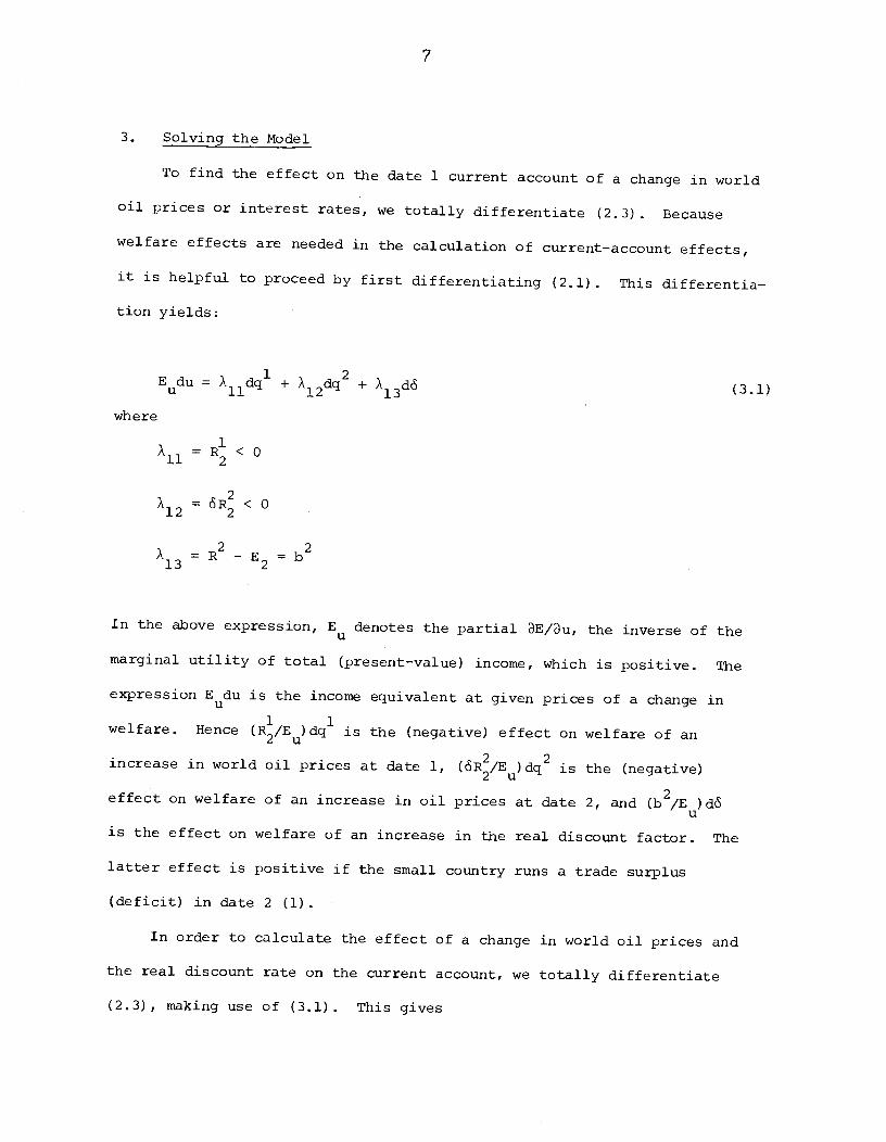
3. Solving the Model

To find the effect on the date 1 current account of a change in world

oil prices or interest rates, we totally differentiate (2.3). Because

welfare effects are needed in the calculation of current—account effects,

it is helpful to proceed by first differentiating (2.1). This differentia-

tion yields:

Edu =A11dq' +

A12dq2 + X13d (3.1)

where

A11 = < 0

A12 = < 0

2 2X13 = R -

E2= b

In the above expression, Eu denotes the partial BE/u, the inverse of the

marginal utility of total (present-value) income, which is positive. The

expression Edu is the income equivalent at given prices of a change in

welfare. Hence (R/E)dq1 is the (negative) effect on welfare of an

increase in world oil prices at date 1, (5R/E)dq2 is the (negative)

effect on welfare of an increase in oil prices at date 2, and (b2/E)dS

is the effect on welfare of an increase in the real discount factor. The

latter effect is positive if the small country runs a trade surplus

(deficit) in date 2 (1).

In order to calculate the effect of a change in world oil prices and

the real discount rate on the current account, we totally differentiate

(2.3), making use of (3.1). This gives

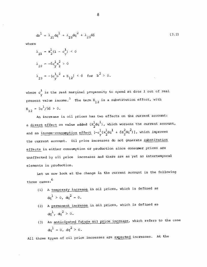
8

db1 =A21dq

+A22dq2

+A23dS

(3.2)

where

A =R1(1- c1) <021 2 y

A =—5c1R2>022 y2

A = -[c1b + E I < 0 for b2 > 0.23 y 12

where c1 is the real marginal propensity to spend at date 1 out of real

present value income.3 The term E12 is a substitution effect, with

E12 = c1/S > 0.

An increase in oil prices has two effects on the current account:

a direct effect on value added (Rdq), which worsens the current account,

and an income-consumption effect [-c1(Rdq1 + SRdq2)], which improves

the current account. Oil price increases do not generate substitution

effects in either consumption or production since consumer prices are

unaffected by oil price increases and there are as yet no intertemporal

elements in production.

Let us now look at the change in the current account in the following

three cases:

(1) A temporary increase in oil prices, which is defined as

dcl' > 0, dq2 = 0.

(2) A permanent increase in oil prices, which is defined as

dq1, dq2 > 0.

(3) An anticipated future oil price increase, which refers to the case

1 2dq = 0, dq > 0.

All three types of oil price increases are expected increases. At the

9

start of date 1, OPEC announces oil prices for dates 1 and 2. Agents can

fully adjust their behavior in dates 1 and 2 in response to this

announcement. Later, we shall distinguish between expected and unexpected

price increases.

As can be seen in (3.2), a temporary oil price increaseunambiguously

reduces the current—accot surplus; it has a direct negative effect on

value added and a smaller positive income effect on demand.

A permanent oil price increase has a larger impact on aggregate

demand and hence an ambiguous effect on the current account. As in the

case of a temporary increase, it has a direct negative effect and a smaller

positive income effect in date 1. But it also produces a positive income

effect in date 2. If the two income effects should dominate, then the

current account will improve.

An anticipated oil price increase improves the date 1 current account

since it lowers welfare, inducing a drop in domestic consumption in the

first period.

Up to this point, agents have been treated as having perfect foresight;

they can fully adjust in dates 1 and 2 to any oil price increase that

occurs in the present or the future.

Suppose we want to introduce a distinction between unexpected and

expected oil price increases. One way to do this is to impose some

constraint on the ability of agents to adjust their behavior in date 1 in

response to an announced oil price increase. In particular, suppose that

firms have limited production substitution possibilities in date 1. Any

change in date 1 oil prices — whether temporary or permanent - is now

unexpected in the sense that firms would have tried to alter their factor

10

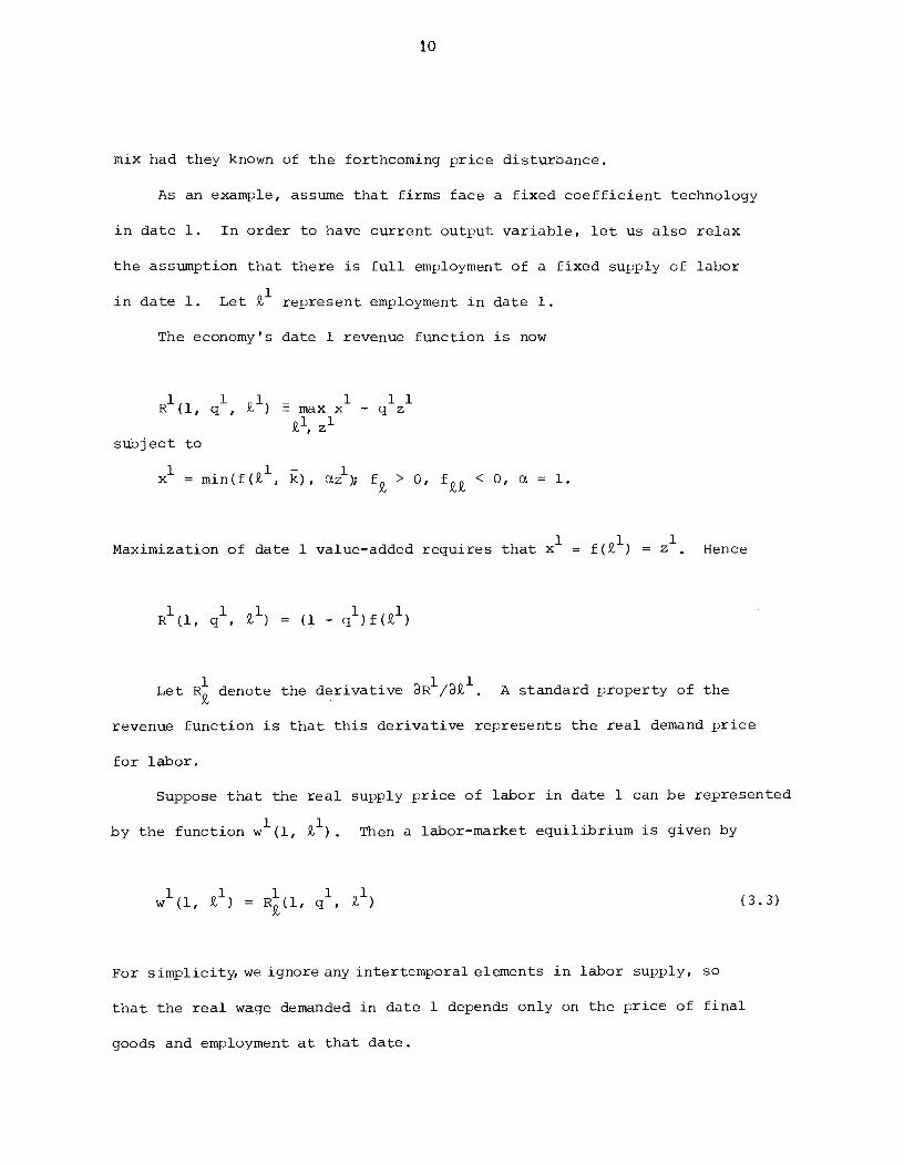
mix had they known of the forthcoming price disturbance.

As an example, assume that firms face a fixed coefficient technology

in date 1. In order to have current output variable, let us also relax

the assumption that there is full employment of a fixed supply of labor

in date 1. Let represent employment in date 1.

The economy's date 1 revenue function is now

1 1 1 — 1 11R (1, q , i ) = max x - q z

l, lsubject to

x1 = min(f(2), k), l) f > 0, f < 0, c = 1.

Maximization of date 1 value-added requires that x1 = f(9)) = z1. Hence

R1(l, q', l) = (1 -

Let denote the derivative A standard property of the

revenue function is that this derivative represents the real demand price

for labor.

Suppose that the real supply price of labor in date 1 can be represented

by the function w'(l, 2)). Then a labor-market equilibrium is given by

w1(l, l) = R(l, q1, i1) (3.3)

For simplicity, we ignore any intertemporal elements in labor supply, so

that the real wage demanded in date 1 depends only on the price of final

goods and employment at that date.

11

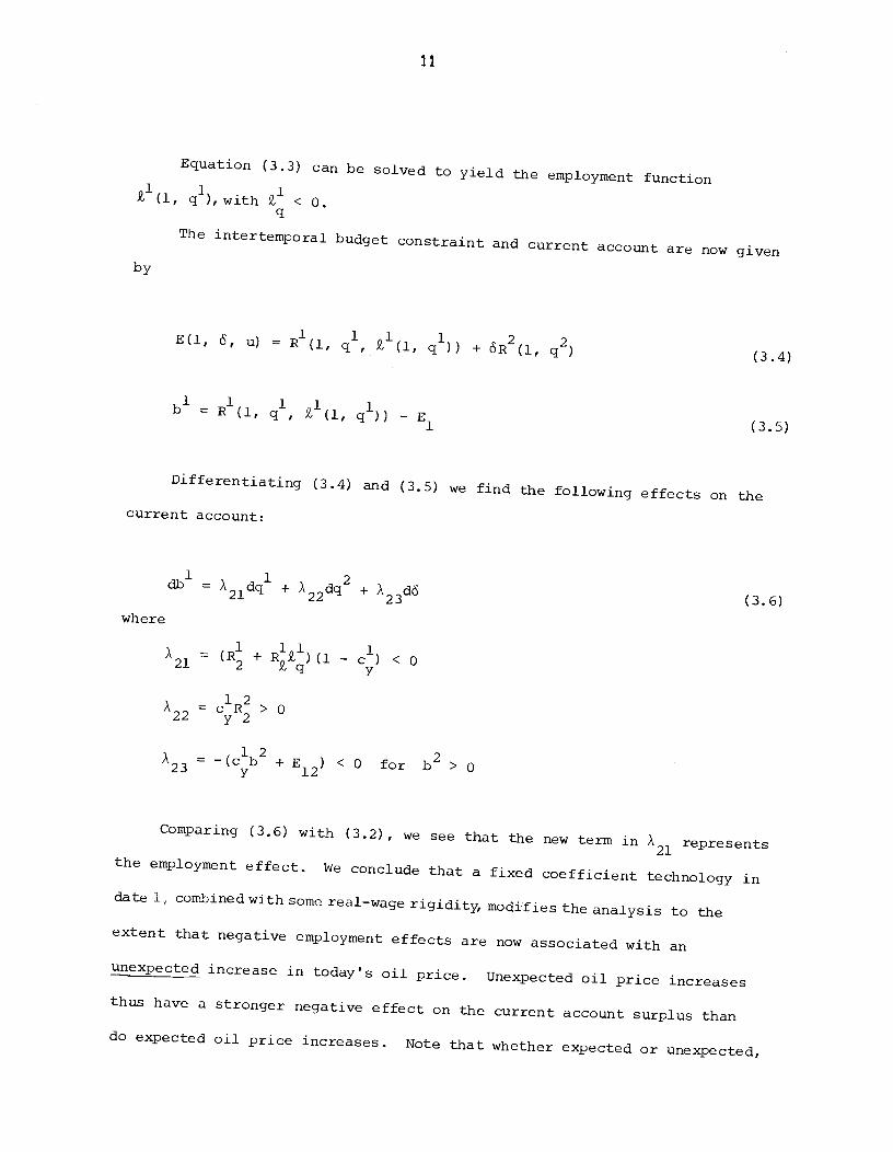
Equation (3.3) can be Solved toyield the employment function

1 1 12 (1, q ), with 9 < 0.

The intertemporal budget constraint and current account are now given

by

E(l, , u) = R1(l, q1, (l q1)) + R2(l q2)(3.4)

b1 = R1(l, q1, l(l q1)) -E1 (3.5)

Differentiating (3.4) and (3.5) we findthe following effects on the

Current account:

=A21dq' + A22dq2 + A23d (3.6)

where

A21 2 lq y

A c1R2>O22 y2

A23 = _(clb2 + E12) < 0 for b2 > 0

Comparing (3.6) with (3.2), we see that the new term in A21 represents

the employment effect. We conclude that a fixed coefficienttechnology in

date 1, combined with some real-wage rigidity, modifies the analysis to the

extent that negative employment effects are now associated with anUnexpected increase in today's oil price. Unexpected oil price increasesthus have a stronger negative effect on the current account surplus thando expected oil price increases. Note that whether expected or unexpected,

12

a temporary increase in oil prices reduces the current-account surplus and

a permanent increase in oil prices has an ambiguous effect on the current

account. Anticipated future oil price increases always improve today's

current account.

Let us now examine how the current—account response might differ when

a nontraded good is introduced.

13

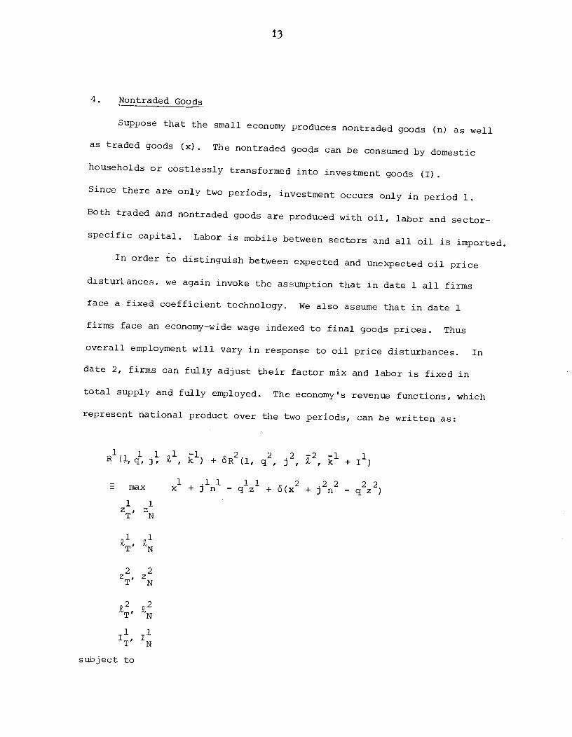
4. Nontraded Goods

Suppose that the small economy producesnontraded goods (n) as well

as traded goods (x). The nontraded goods can be consumed by domestic

households or costlessly transformed into investment goods (I).

Since there are only two periods,investment occurs only in period 1.

Both traded and nontraded goodsare produced with oil, labor and sector-

specific capital. Labor is mobile between sectors and all oil is imported.

In order to distinguish betweenexpected and unexpected oil price

disturLances, we again invoke the assumption that in date 1 all firms

face a fixed coefficient technology. We also assume that in date 1

firms face an economy—wide wage indexed to final goods prices. Thus

overall employment will vary in response to oil price disturbances. In

date 2, firms can fully adjust their factor mix and labor is fixed in

total supply and fully employed. The economy's revenue functions, whichrepresent national product over the two periods, can be written as:

R1(i c, J; l k1) + R2(l, q2, 2 2 jl + Ii)— 1 .11 11 2 .22 22= max x +Jn -qz +(x +jn -qz)

1 1z, zT N

1 1'T'

2 2z, zT N

2,2 2,2T N

1 1''IT N

subject to

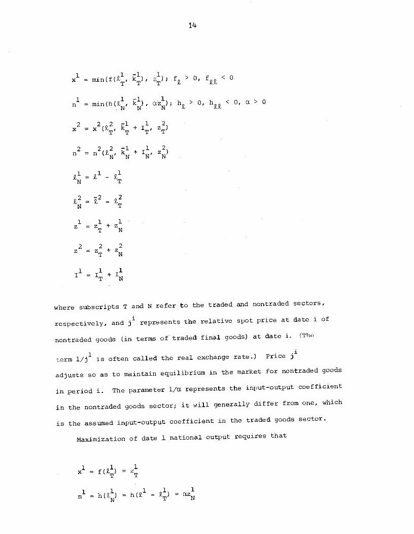
14

= min(f(9, k), z); f > 0, f < 0

n1 = min(h(9, kH, cz:hi; h > 0, h < o, c > 0

2 2 2 —1 1 2= T' kT + 'T' zT)

2 2 2 —1 1 22N' k + 'N' ZN)

= 1 -N T

= —

N T

l 1 1Z =Z +Z

T N

2 2 2Z =ZT+ZN

Ii = I +

where subscripts T and N refer to the traded and nontraded sectors,

respectively and j1 represents the relative spot price at date i of

nontraded goods (in terms of traded final goods) at date i. (The

term l/j1 is often called the real exchange rate.) Price

adjusts so as to maintain equilibrium in the market for nontraded goods

in period i. The parameter 1/ct represents the input-output coefficient

in the nontraded goods sector; it will generally differ from one, which

is the assumed input-output coefficient in the traded goods sector.

Maximization of date 1 national output requires that

1 1 1x =

= h(Z) = h( - ) =

15

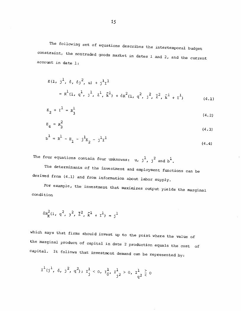
The following set of equations describes theintertemporal budget

constraint, the nontradedgoods market in dates 1 and 2, and the current

account in date 1:

.1 .2 .11E(l, j , , cSj , u) + j I

1 1 .1 1 —l 2 2 2 —2 —l 1= R (1, q , j , , k ) + SR (1, q , j , , k + I ) (4.1)

E2 + =

(4.2)

E4(4.3)

bl=R1_El_j1E_jlIl(44)

The four equations containfour unknowns: u, j1, j2 and b'.

The determinants of the investment and employment functions can be

derived from (4.1) and from information about labor Supply.

For example, the investmentthat maximizes Output yields the marginal

condition

SR(l, q2, 2 2 + Ii) =

which says that firms should investup to the point where the value of

the marginal product of capital in date 2 production equals the cost of

capital. it follows that investment demand can be represented by:

, j2, q2); i < O I, 12 > O 12

16

It is a function of the cost of capital, j1, the prices of date 2 final

goods, 5 and 2, and the date 2 price of oil. Since 5 l/(1 + r), the

investment function captures the familiar relationship between the

real interest rate and investment demand. Changes in the date 1 price

of oil affect investment demand indirectly through j1 and by influencing

the supply of investment goods.7 The properties of the investment function

can be obtained from information about the production technology. Given

a convex production technology in date 2, it can be shown that an increase

in the price of capital goods decreases investmentdemand while an

increase in date 2 final prices raises the marginal product of capital

and hence investment demand. An increase in date 2 oil prices lowers

investment demand if capital and oil are complements in date 2 production

and increases investment demand if the two factors are substitutes.

The employment function, S, can be derived from the labor-market

equilibrium condition:

1 1 .1 1 —l 1 .1 1

R(l, q, j , Z, k) =w (1, j , 5)

It follows that

1 .1 1 1> 12 (1, j , q ); 9. o 1

< 03 q

An increase in raises employment in the nontraded goods sector and

lowers it in the traded goods sector, so there is an ambiguous impact on

economy-wide employment in date 1. An increase in q1 lowers the net

marginal product of labor in both sectors and hence reduces overall

employment in the current period.

Having discussed some of the properties of the model, we are now ready

to analyze the effects of oil price increases on the current account when

the economy produces both traded goods and nontraded consumer and/or

17

investment goods.

First, totally differentiate (4.l)—(4.4).Equation (4.1) can be

solved separately to obtain the welfare effects of oil price increases.

Equations (4.2) and (4.3) must be solved simultaneously to obtain

equilibri values for the price of nontraded goods in dates 1 and 2.

The solutions to (4.l)—(4.3) can then be used in (4.4) to obtain the

current—accot effects of oil price increases.

The welfare and current—account effects are as follows:

Edu =X11dq1 +

A12dq2 + X13d + X14dj1 (4.5)where

1 ii=R2

+R;Zq

< o

A12=

5R < 0

A13 = b2

A14 R22— 0

=A21dq1

+A22dq2 + A23d +

A24dj1 + A25dj2 (4.6)

where

A = (R1 + RQ1) (1 — c1) < 021 2 iq y

A = — c5R2 > 0 if I < 022q2 y 2

q2

12 .2 1 .12 .11 >A23

= —(cb +E13

+ j E14 +j E23+ j j E + j I) 0

A24 = R11(l - c1) -E12

—j1E22

— 0

A25= l4 + 24 + 0

18

Equations (4.5) and (4.6) have been written in the above form even

though j1 andare endogenous variables in order to highlight the

channels through which oil price increases alter welfare and the current

account. Clearly, oil price increases affect welfare and the current

1account both directly, through q and q', as well as indirectly, through

their influence on nontraded goods prices j1 and j2.

4.1 The role of nontraded investment goods

In order to see clearly how these channels operate,consider first

the case where the only nontraded goods produced are investment goods,

and all investment takes place in date 1.This simplified case can be

represented by equations (4.7)—(4.9),which are a modification of equations

(4.l)-(4.4):

E(l, , u) + j111 = R1(1, q1, j1, 1 k1) + R2(1, q2, 2 l + Ii) (4.7)

I =(4.8)

b1 = — E1 — j111(4.9)

The investment and employment functions are now given by:

11(j1, , q2); I < 0,I > OF I <0

l(l ' q; l > Of 1l < 0j q

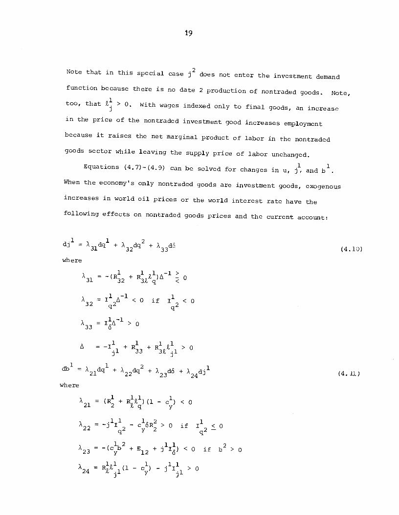
19

Note that in this special case j2 does not enter the investment demand

function because there is no date 2 production of nontraded goods. Note,

too, that > 0. With wages indexed only to final goods, an increase

in the price of the nontraded investment good increases employment

because it raises the net marginal product of labor in the nontraded

goods sector while leaving the supply price of labor unchanged.

1 1Equations (4.7)-(4.9) can be solved for changes in u, j, and b

When the economy's only nontraded goods are investment goods, exogenous

increases in world oil prices or the world interest rate have the

following effects on nontraded goods prices and the current account:

dj1 =A31dq1 +

A32dq+ A33d (4.10)

where

1 1 1 —1>131 = —(R32

+R3q)A 0

A =11A1<o if I <032 q2

133 = iA > 0

A = + R3 + R211 > 0

=A1dq1 + X2dq2 + A23d + A24dj' (4.11)

where

A = l + R1) (1 — c1) < 021 2 q y

A = — cSR2 > 0 if < 022q2 y 2 q2

123 = —(c1b2 + E12 + j1I) < 0 if b2 > 0

124 = R51(1 — c1) — > 0

20

A temporafy increase in oil prices affects the supply of investment

goods but not the demand. The disturbance can either raise or lower

nontraded goods prices, depending on the relative oil intensity of

production in the two sectors of the economy. Technically, the response

of j1 depends on the sign and size of R2 in A31. The term represents

the supply response in the nontraded goods sector to an increase in date

1 oil prices for a given economy—wide level of employment. If a

temporary increase in date 1 oil prices reduces the supply of nontraded

investment goods (R2 < 0), then j1 will rise. The resulting drop in

investment demand helps improve the current account (A24 > 0). Note that

the current account is also helped by the small drop in household

absorption induced by the oil shock. But since temporary oil price increases

also have a direct negative effect on GNP (R < 0 in A21), their net impact

on the current account is ambiguous. Only if temporary oil price increases

reduce the relative price of nontraded goods will the current account

clearly deteriorate. Recall that in the absence of nontraded goods,

temporary oil shocks always led to a current-account deterioration.

Temporary oil price increases are more likely to increase the supply

of nontraded goods and reduce their price the lower the oil—value—added

ratio (the greater the c*) in the nontraded goods sector relative to the

traded goods sector.9 That is because under such circumstances an

increase in oil prices will induce a movement of labor from traded to

nontraded goods. Temporary oil price increases which are unexpected

also generate additional employment effects in both sectors when there

is real-wage resistance.

Permanent oil price increases alter both the demand and the supply

of nontraded investment goods and have an ambiguous effect on their

21

price. As in the previous case, the supply of investment goods will

rise or fall depending on the relative oil intensity of capital goods

production. A permanent increase in oil prices will also reduce

(increase) the demand for investment goods if oil and capital arecomplements (substitutes) in date 2 production.

Permanent oil price increases have an ambiguous effect on the

current account as well. For given prices of nontraded goods, they

reduce GNP and employment (R + < 0 in A21), which worsens the

current account. They lead to a cut in absorption, which improves the

current account; the expressions (R1 + RQ1) (—c1) in A and R2(—c1)2 q y 21 2 yin A22 indicate that consumer expenditures fall and the term -j1I'2inA shows

q 22

that investment demand drops if capital and oil are complements in date

2 production. But prices of nontraded goods do not remain fixed. As

we have seen, permanent oil price increases can either raise or lower

nontraded goods prices. If j' should increase, we see from A24 that

employment is stimulated and investment demand is further reduced. The

spur to output and the fall in absorption help improve the current

account. If should fall, there is instead an additional negative

effect on the current account.

An anticipated future increase in oil prices reduces (increases)

the demand for investment goods if capital and oil are complements

(substitutes) in date 2 production, but has no effect on their current

supply. Consequently, the expected future disturbance reduces (increases)

today's relative price of nontraded goods.

When oil and capital are complements in date 2 production, an

anticipated future increase in oil prices improves the date 1 current

account. It can be shown that when 112 < 0, the expression [X22dq2+A2432dq2j

22

in (4.11) is unambiguously positive. The anticipated future increase in

oil prices reduces permanent income, leading households to cut their expend-

itures in both periods. The expected increase also lowers the relative

price of capital goods, j1, with a resulting drop in employment. This

additional welfare loss also induces households to reduce their spending.

Finally, since the drop in j1 triggers a contraction of employment in

the nontraded goods sector, there is a concomitant drop in the demand for

oil imports, given the fixed coefficient technology in place in date 1.

All of these responses contribute to an improved current account.

Recall that anticipated future oil price increases always led to an

improved current account when the economy produced just traded goods.

The introduction of nontraded investment goods, however, permits oil

price increases to influence the current account through additional

channels. As we have seen, anticipated future oil price increases

unambiguously improve the current account if capital and oil are

complements in date 2 production.

The inclusion of nontraded goods highlights the importance of the

oil—value—added ratio in the nontraded goods sector relative to the

traded goods sector in determining the current-account response to current

oil price increases. The relative oil intensity of production will also

be an important determinant of the current-account response to anticipated

future oil price increases once we introduce nontraded consumer goods

and hence nontraded goods production in both periods.

4.2 The role of nontraded consumer goods

Consider next the case where the small economy's only nontraded good

is a consumer good. Then the general model represented by equations

(4.1)-(4.4) can be modified as follows:

23

.1 .2 1 1 1 1—1 2 2 2—2—1E(l, j , S, S , U) = R (1, q , j , , k ) + R (1, q , j , , k ) (4.12)

E2 =(4,13)

E4 =(4.14)

1 1 1b = R -E1

- j E2 (4.15)

The employment function is now given by:

9,1(1 j1, q1); 2, 0, < 0

Its properties are identical to the employment function of the general model.

There is no investment function.

Equations (4.12)-(4.15) can be solved for changes in u, j', j2 and

b1. When the economy's only nontraded good is a final good, exogenous

increases in world oil prices or interest rates'1havethe following effects

on nontraded goods prices and the current account:

1 1 2dj =A31dq

+k32dq

+A33d (4.16)

where

= {[R2 + R39,l -cyN(R2 + R2)J [E44 - R3]

+ 2 (R1 + R11)E }V1 0yN 2 9,q 24

X32=

{_c1NR(E44-

R33)+ (-R2 +

cNR2)E4}V 0

.2 1 2 2A33 = {—tE23

+ J E24 +CyNb

) (E44—

R33)

+(-R

+E43

+j2E44

+cNb)E24}V o

24

—R 9 +c R)V=(E -R2)(E -R1 1 1 1 139j yNj44 33 22 33

—E24(E

+ C2 R19)) > 042 yNj

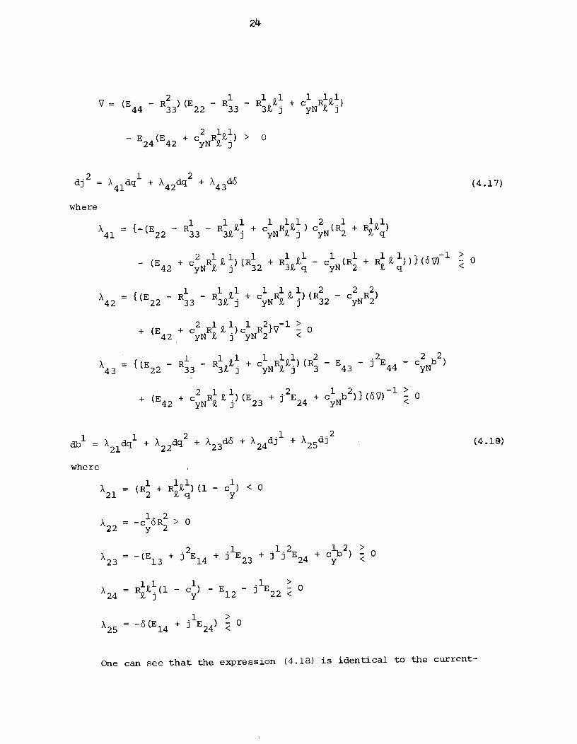
dj2 =A41dq1

+ A42dq2+ X43d (4.17)

where

1 1 11 2 1+c R9 )c (R +RS)A41 = {-E22-

R3-

yN 9, j yN 2

- CE + C2 R1i)(R1 + R1 9,1 - c1 CR1 + R11))}(OV)1>

42 yN j 32 32,q yN 2 q <0

X42={(E22—R3—R991 1 1 2 2 2+c R9)(R —c R)yN j 32 yN2

+ (E + C2 RQ1)c1 R2}V1 042 yN j yN2

A43=

{(E22-

R3— R2 + C1 RL) (R — E43

—j2E44

—CNb)yN 9, j

+ (E4 + C2 R19)(E23 + j2E24 + C1 b2)}(V) 1

yN2 yN j

=X21dq1

+ A22dq+ X23d + A24dj1 + A25dj2 (4.19)

where

A21 = (R + R1)(1 — c1) < 0

12A =—cR >022 y 2

1 212>A23 = -(E13 +JE14+JE23 + j j E24 + c b ) 0

y <

=R9, (1—c) -E —jE -0A24

1 1 >

2,j y 12 22<

1 >A25 = —S(E1 + j E24) 0

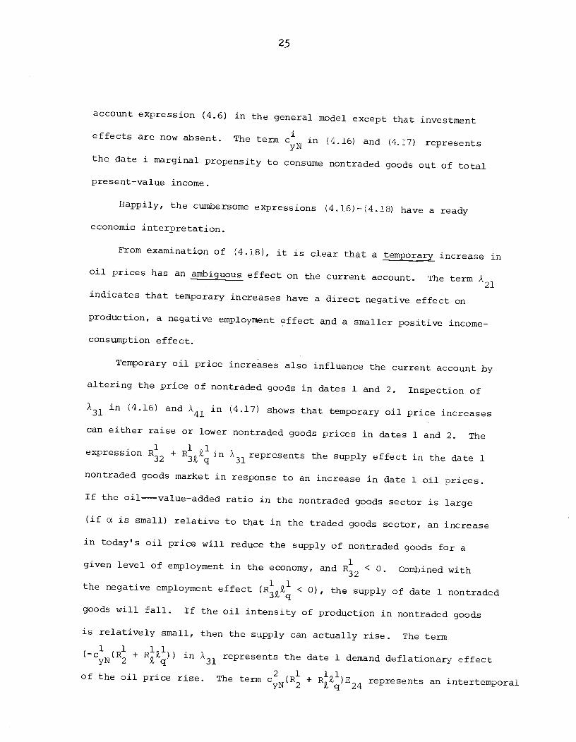
One can see that the expression (4.18) is identical to the current-

25

accoui-it expression (4.6) in the general model except that investment

effects are now absent. The term C in (4.16) and (4.17) representsthe date i marginal propensity to consume nontraded goods out of total

present—value income.

Happily, the cumbersome expressions (4.16)-(4.18) have a ready

economic interpretation.

From examination of (4.18), it is clear that a temporary increase in

oil prices has an ambiguous effect on the current account. The term'2l

indicates that temporary increases have a direct negative effect on

production, a negative employment effect and a smaller positive income-

consumption effect.

Temporary oil price increases also influence the current account by

altering the price of nontraded goods in dates 1 and 2. Inspection of

X31 in (4.16) and in (4.17) shows that temporary oil price increases

can either raise or lower nontraded goods prices in dates 1 and 2. The

expression + in X31 represents the supply effect in the date 1

nontraded goods market in response to an increase in date 1 oil prices.

If the oil—value-added ratio in the nontraded goods sector is large

(if c is small) relative to that in the traded goods sector, an increase

in today's oil price will reduce the supply of nontraded goods for a

given level of employment in the economy, and R2 < 0. Combined with

the negative employment effect (R9 < 0), the supply of date 1 nontraded

goods will fall. If the oil intensity of production in nontradedgoods

is relatively small, then the supply can actually rise. The term

(—c1 (R1 + R')) in A represents the date 1 demand deflationary effectyN 2 £q 31

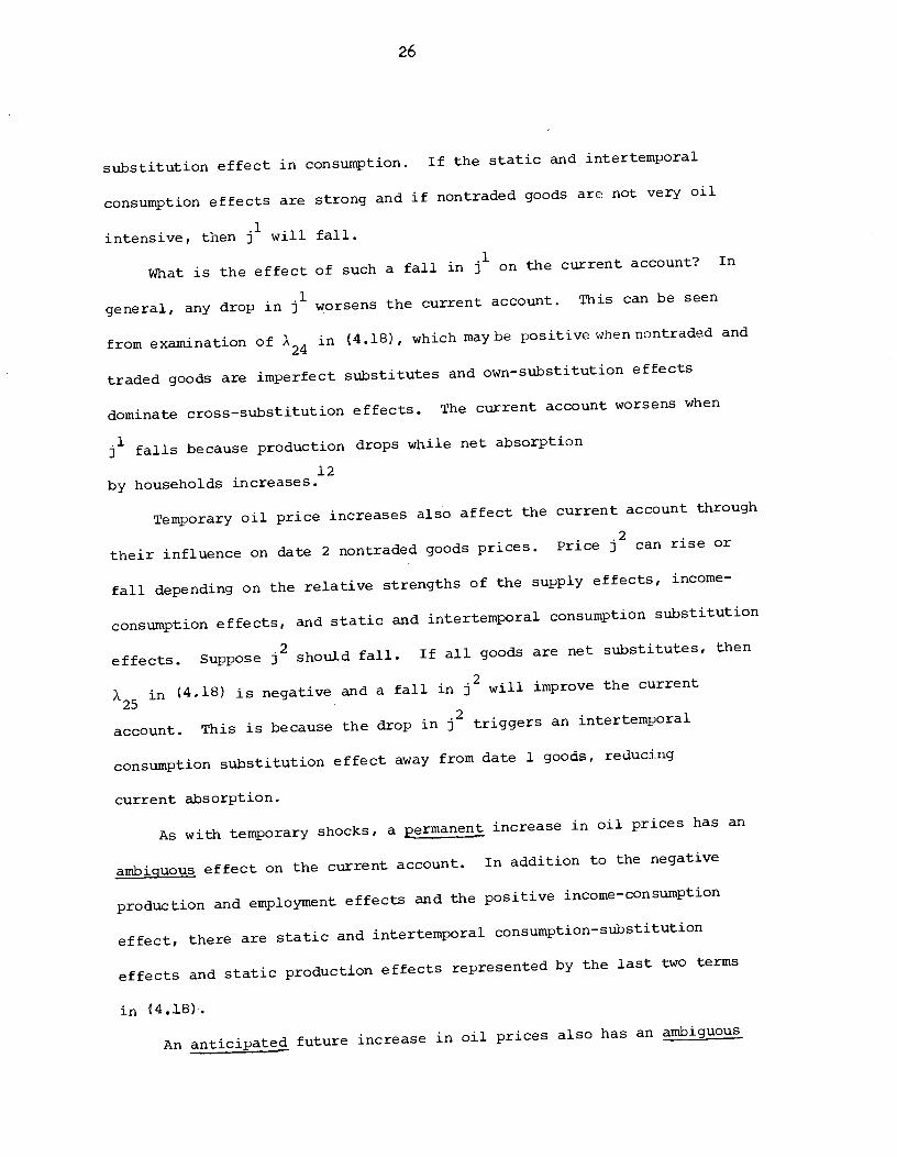
of the oil price rise. The term C2 (R1 + R1)E represents an intertemporalyN 2 q 24

26

substitution effect in consumption. If the static and intertempOral

consumption effects are strong and if nontraded goods are not very oil

intensive, then will fall.

What is the effect of such a fall in on the current account? In

general, any drop in worsens the current account. This can be seen

from examination of in (4.18), which maybe positive whennontraded and

traded goods are imperfect substitutes andown—substitution effects

dominate cross—substitution effects. The current account worsens when

falls because production drops while net absorption

by households increases.

Temporary oil price increases also affect the current account through

their influence on date 2 nontraded goods prices. Price can rise or

fall depending on the relative strengths of the supply effects, income-

consumption effects, and static and intertempOral consumption substitution

effects. Suppose should fall. If all goods are net substitutes, then

A25 in(4.18) is negative and a fall in will improve the current

account. This is because the drop in triggers an intertemPoral

consumption substitution effect away from date 1 goods, reducing

current absorption.

As with temporary shocks, a permanent increase in oil prices has an

effect on the current account. In addition to the negative

production and employment effects and the positive income-consumption

effect, there are static and intertemporal consumption_substitution

effects and static production effectsrepresented by the last two terms

in (4.18).

An anticipated future increasein oil prices also has an ambiguo

27

effect on the current account. In addition to the positive income—

consumption effect, A22, in (4.l8), expected future increases in oil

prices may raise or lower nontraded goods prices in dates 1 and 2, making

the last two terms in (4.18) of either sign.

Again, the response of nontraded goods prices depends crucially on

the relative oil intensity of nontraded goods production. The term

in both A32 andA42 represents the supply effect in the nontraded

goods market in date 2 following an increase in date 2 oil prices. The

smaller the oil intensity of production in the nontraded goods sector

relative to the traded goods sector, the more likely that R2 will be

positive. Indeed, if the nontraded good uses no oil inputs in date 2

production, and given that labor is fixed in supply and fully employed

in date 2, an expected future oil price increase will only induce a

movement of labor from traded to nontraded goods. will be positive.

Consequently A32 in (4.16) is negative, A42 in (4,17) is likely to be

negative, and we can say that expected future oil price increases will

lower the relative price of nontraded goods in dates 1 and 2.

We know that a fall in j1 tends to worsen the current account while

a fall in tends to improve it. Consequently, we cannot ascertain the

net impact on the current account of anticipated future oil priceincreases without knowledge of specific parameter values, includingthe relative oil intensity of production in the traded and nontraded

sectors.

Comparing the results in Section 4.2 with those in Section 3, wesee that the current—accouit response to various types of oil priceincreases are much less clear cut once we introduce nontraded goods and

28

the possibility of intertemporal and static substitution effects in

consuiript ion.

29

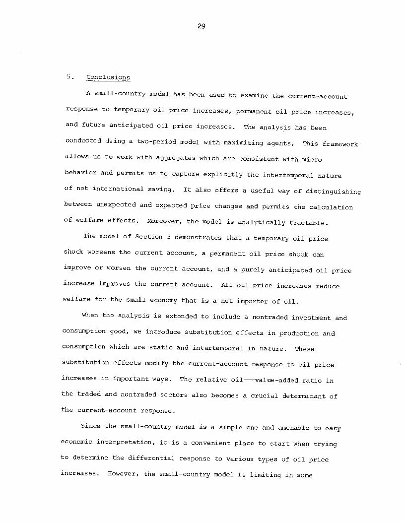
5. Conclusions

A small—country model has been used to examine the current—account

response to temporary oil price increases, permanent oil price increases,

and future anticipated oil price increases. The analysis has been

conducted Using a two—period model with maximizing agents. This framework

allows us to work with aggregates which are consistent with micro

behavior and permits us to capture explicitly the intertemporal nature

of net international saving. It also offers a useful way of distinguishing

between unexpected and expected price changes and permits the calculation

of welfare effects. Moreover, the model is analytically tractable.

The model of Section 3 demonstrates that a temporary oil price

shock worsens the current account, a permanent oil price shock can

improve or worsen the current account, and a purely anticipated oil price

increase improves the current account. All oil price increases reduce

welfare for the small economy that is a net importer of oil.

When the analysis is extended to include a nontraded investment and

consumption good, we introduce substitution effects in production and

consumption which are static and intertemporal in nature. These

sUbstitution effects modify the current—account response to oil price

increases in important ways. The relative oil—value—added ratio in

the traded and nontraded sectors also becomes a crucial determinant of

the current—account response.

Since the small—country model is a simple one and amenable to easy

economic interpretation, it is a convenient place to start when trying

to determine the differential response to various types of oil price

increases. However, the small—country model is limiting in some

30

respects. For instance, its partial—equilibrium nature ignores the

feedback effects of higher oil prices on traded goods prices and world

interest rates that have been stressed in the two-country model of

Sachs (1980) and the three—country model of Marion-Svensson (1981).

The model described here should be seen as offering a useful way to

analyze the effects of expected versus unexpected disturbances on

important macro variables, but should be viewed as a first step in

developing a more complete general equilibrium analysis.

F-i

Footnotes

Helpful comments from Robert Flood, Dale Henderson, Meir Kohn,Lars Svensson and the seminar participants at the Board ofGovernors of the Federal Reserve System are gratefullyacknowledged.

similar intertemporal framework that employs the dual approachcan be found in Svensson and Razjn (1981). See also Dixit and Norman(1980)

2For a model where prices of traded goods and world interest rates

are determined endogenously as part of a general equilibrium system,see Marion and Svensson (1981).

is the present—value price of date 2 final goods in terms ofthe date 1 price of final goods.

4By assumption there is no foreign debt initially, so there are nointerest payments in the current account at date 1. The current accountat date 1 is equal to the trade balance.

5Alternatively, c is the partial derivative with respect to present-value income of the Marshaflian

uncompensated demand for goods at date 1.

6The distinction between temporary, permanent and future eecteddisturbances has been made by Svensson and Razin (1981) in theirintertemporal analysis of the effect.

71n Sachs (1981), investment is determined solely by the exogenously-given world interest rate (our , where F 1/(1 + r)), and by date 2oil prices. Consecjuently, temporary oil price disturbances have noeffect on investment. Further, domestic variables cannot influenceinvestment. In our model, by contrast, temporary oil price increasesindirectly alter the demand for investment goods by changing their price.In addition, exogenous or policy-induced domestic disturbances, thoughnot explicitly modeled, can alter the relative price of nontraded goodsand thereby influence investment behavior. Moreover,

forein disturbancesinfluence investment demand not only directly, through , qr and q , butindirectly, through j' and j2.

F-2

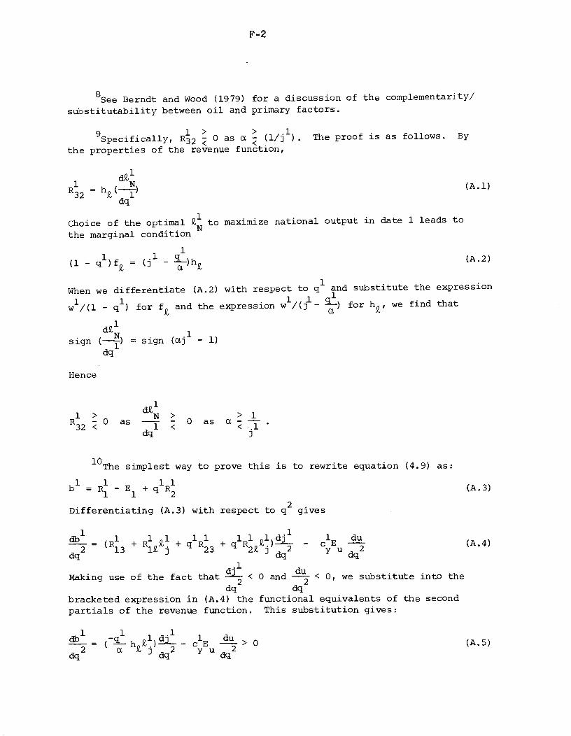
8See Berndt and Wood (1979) for a discussion of the complementarity/substitutability between oil and primary factors.

9 1> > .1Specifically, R32 0 as 0. (l/j ) . The proof is as follows. By

the properties of the revenue function,

1 NR32 = h,(—1-)

(A.l)

dq

Choice of the optimal to maximize national output in date 1 leads to

the marginal condition

(1 - q1)f = (j1 - -)h (A.2)

When we differentiate (A.2) with respect to q1 and substitute the expression

w1/(1 - q1) for f and the expression w1/(j1- -) for hi,, we find that

d9) 1sign (—-) = sign (0.j - 1)

dq

Hence

s,11> dN > >1R32O as —i- 0 as

dq j

10The simplest way to prove this is to rewrite equation (4.9) as:

b1=R-E1+q1R (A.3)

Differentiating (A.3) with respect to q2 gives

=(R3 + R2 + q1R3 + qlRll)J__ - c1E

d2(A.4)

Making use of the fact that < 0 and --- < 0, we substitute into the

bracketed expression in (A.4) the functional equivalents of the secondpartials of the revenue function. This substitution gives:

1 1 .1

= (i— h 9))----- - c1E —--- > 0 (A.5)

dq2 c Jdq2 Yhldq2

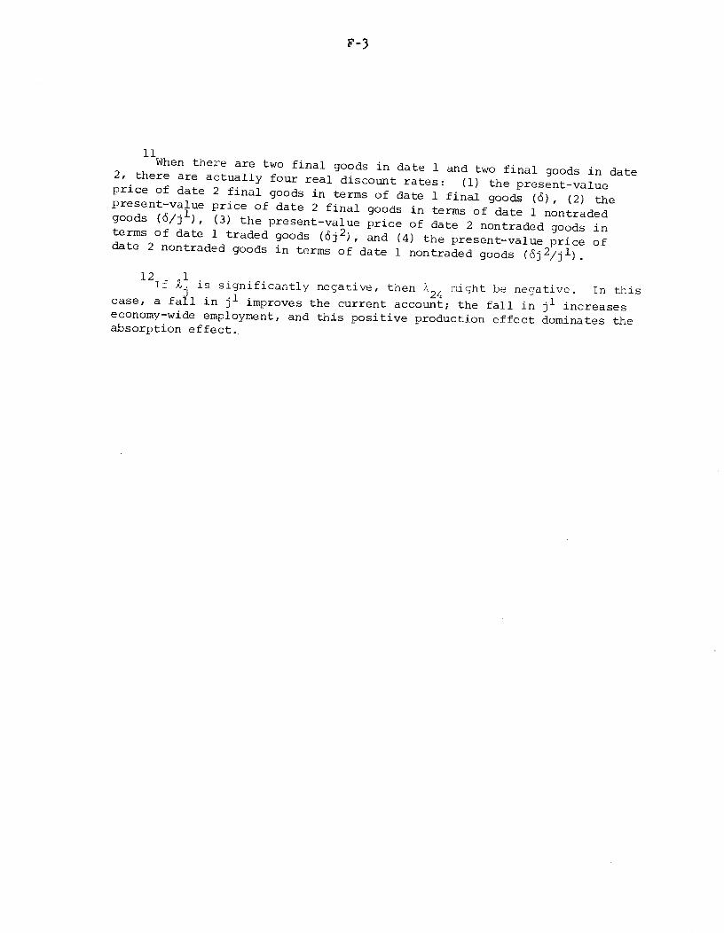
F-3

11When there are two final goods in date 1 and two final goods in date2, there are actually four real discount rates: (1) the present-valueprice of date 2 final goods in terms of date 1 final goods (5), (2) the

present-value price of date 2 final goods in terms of date 1 nontradedgoods (/j1), (3) the present-value price of date 2 nontraded goods interms of date 1 traded goods (cSj2), and (4) the present—value price ofdate 2 nontraded goods in terms of date 1 nontraded goods (j2/jJ)•

l2 is significantly negative, then A24 might be negative. In thiscase, a fail in j' improves the current accot; the fall in j1 increaseseconomy-wide employment, and this positive production effect dominates theabsorption effect.

a-i

References

Berndt, E. and D. Wood (1979). Engineering and Econometric Interpretations

of Energy—capital ComplementaritY,7merican Economic Review, June,

342-354.

Bruno, M. and J. Sachs (1978) . Macroeconomic Adjustment with Intermediate

Imports: Real and Monetary Aspects, Institute for International

Economic Studies Seminar Paper No. 118, Stockholm.

Buiter, W. (1978). Short-run and Long-runEffects of External Disturbances

Under a Floating Exchange Rate, Economica 45, August, 251-272.

DiXit, A. (1980). An Introduction to Duality Theory and Applications,

mixneo.

Dixit, A. and V. Norman (1980). Theory of International Trade, cambridge

University Press, London.

Findlay, R. and RodrigUez (1977).Intermediate Imports and Macroeconomic

Policy Under Flexible Exchange Rates, Canadian Journal of Economics

10, May, 208—217.

Katseli, L. and N. Marion (1980). Adjustment to Variations in Imported

Input Prices: The Role of Economic Structure, NBER Working Paper

No. 501.

Marion, N. and L. Svenssofl (1981) . Oil Price Increases and Macroeconomic

Adjustment in a Three-Country Model, mimeO.

Obstfeld, M. (1980). Intermediate Imports,the Terms of Trade, and the

Dynamics of the Exchange Rate and Current Account, Journal of

International EconomicS, November, 461-480.

R -2

Sachs, J. (1980). Energy and Growth under Flexible Exchange Rates: A

Simulation Study, NBER Working Paper No. 582.

____ (1981) . The Current Account and Macroeconomic Adjustment in

the l970s, Brookings Papers on Economic Activity, Volume 1.

Svensson, L. and A. Razjn (1981). The Terms of Trade, Spending and the

Current Account: The Harberger- Laursen- Metzler-Effect, Institute

for International Economic Studies Seminar Paper No. 170, Stockholm.

Varian, H. B. (1978). Microeconomic Analysis, Norton, New York.