NBER WORKING PAPER SERES

HAS WORK-SHARING WORKED IN GERMANY?

Jennifer Hunt

Working Paper 5724

NATIONAL BUREAU OF ECONOMIC RESEARCH1050 Massachusetts Avenue

Cambridge, MA 02138August 1996

I thank Alison Booth, Ed kear, Dan Hamermesh, Michael Lechner, John Pencavel, Joel Waldfogeland seminar participants at Stanford and the ZEW (Mannheim) for suggestions. Reinhard Bispinckprovided me with essential information, and Tomas Rauberger was invaluable in setting up theGSOEP data. This research was conducted while I was a National Fellow at the Hoover Institution.This paper is part of NBER’s research program in Labor Studies. Any opinions expressed are thoseof the author and not those of the National Bureau of Economic Research.

@ 1996 by Jennifer Hunt. All rights reserved. Short sections of text, not to exceed two paragraphs,may be quoted without explicit permission provided that full credit, including O notice, is given tothe source.

“About one third of the 3.2 million person increase in employment between 1983 and 1992 canbe attributed to the reduction in working hours. “

“me average standard yearly working time in the Federal Republic was [...] 1669.7 hours in1994. An employment-oriented reduction and flexibilization of standard working hours must aimto reduce this to [...] 1350 hours by 2005. “

Gennun government employment reports (Senatsvetvaltung fir Arbeit und Frauen 1995a, b)

There is a wide-spread popular belief that unemployment can be reduced by reducing the

number of hours worked per person. The reasoning is usually based on what is sometimes

called the “lump of work fallacy”: labor input is seen as fixed, and it is believed that if each

worker works fewer hours, this work can be spread over more workers, and employment will

rise. This is known as work-sharing. However, if restrictions on hours make labor less

attractive to employers, they will substitute to other inputs, and there will also be a scale effect

reducing use of all inputs

Interest in work-sharing resurfaces periodically in different countries, and has been

particularly high in Europe in recent years, following the rise in unemployment since the

mid- 1970s. The tool of choice in Europe for the reduction of working hours is a reduction in

the standard work week: that is, a reduction in the number of hours beyond which an overtime

premium must be paid. The French and Belgian governments mandated reductions in the

standard work week in the 1980s, while German unions have achieved more far-reaching

reductions on an industry by industry basis. In 1996 the French government is threatening to

reduce standard hours further from the current 39 if employers and unions do not agree amongst

themselves to do so. In the United States mandated overtime premia have been preferred as an

inducement to work-sharing (the 50% premium is higher than typical premia in Europe), but the

1

AFL-CIO in 1996 began a campaign for a 32-hour 4-day work week. The use of standard hours

as an hours-reducing tool introduces further ambiguity into the theoretical problem, however,

since employers have the option of shifting to using more overtime.

Most studies of reductions in standard hours have relied on aggregate time series, where

the effect of falling standard hours could be confounded with the effect of another variable

trending down. In this paper I take advantage of the industry level variation in standard hours

reductions in (West) Germany to identify the impact on employment, focusing particularly on

the 1980s. The reductions began with the metal-working and printing sectors in 1985, where

standard hours fell in steps from 40 to 37 between 1984 and 1989. Most other sectors had a

smaller reduction beginning later, while some sectors had no reductions in this period.

Only one econometric study of this episode has been carried out, a study using aggregate

time-series. I use data on 201 manufacturing industries to look at employment directly, and

individual-level data on all industries from the German Socio-Economic Panel to examine layoff

probabilities. Employer-initiated changes in employment stem from changes in hiring or layoff

rates, so at least one part of the process may be examined at a micro-level (hiring rates are

harder to study with individual data).

My results provide a less positive assessment of work-sharing than most of the existing

literature. Industry and individual level data indicate that employment increased by 0.3-0.7%

for hourly workers (Arbeiter) and by 0.2-0.3% for salaried workers (Angestellten) in response

to a one hour fall in standard hours. However, the implied aggregate employment rise of at

most 1.1 % from 1984-89 is small compared with the U.S. employment growth over the same

period (7. 3 % growth in the employment to population ratio), which is arguably the target for

2

the slower German employment growth (3.2% growth in the employment to population ratio).

Furthermore, reductions in standard hours led to large falls in total hours worked, and hence

possibly output losses: a one hour reduction in standard hours was associated with a 2-3% fall

in worker-hours for hourly-paid workers. Workers as a whole did appear to gain from the hours

reductions, however, as the wage bill rose for both hourly-paid and salaried workers. The first

phase of work-sharing thus apparently worked in the sense that employment rose and workers

as a group gained in terms of income and leisure. But employment did not rise enough to

redress Germany’s employment growth problem, and the large falls in worker-hours suggest that

output losses may have occurred. Results for the 1990-94 period are more pessimistic.

Hours Reductions in Gennuny

Unions in Germany bargain at the industry level, and conditions of union contracts apply

not only to members, but to almost all other workers as well. Amual hours may be reduced

either by increasing holiday time or by reducing standard weekly hours. By 1975 the prevailing

conditions were 40 hours per week and 30 days amual leave, and by 1981 95% of workers had

a standard working week of 40 hours’. The metal workers’ union, IG Metall, which along with

the printing union IG Druck had spearheaded earlier reductions in weekly hours, struck

unsuccessfully in 1978-9 to reduce standard weekly hours below 40. Other unions, such as IG

Chemie, the chemical union, focused on reducing life-time hours by reducing the retirement age.

IG Metall resumed its demands in 1982-3, and was successful after a protracted strike in early

1984. The declared aim of the hours reductions was a reduction in unemployment through

3

work-sharing. Hours in the metal-working sector (employing almost four million workers) were

reduced to 38.5 in 1985.

A key element of the agreement, upon which agreements in many other sectors were

modelled, was the concession to employers of greater flexibility in the use of standard hours.

In particular,

could in fact

standard hours no longer had to be spread evenly over each day of the week, and

vary from week to week as long as they averaged to the agreed number over a

certain number of months. 2 Also, standard hours could vary across employees as long as they

averaged to the agreed number. It is important to note that the implementation of flexibility is

a matter to be negotiated at the plant level between the management and the works council, and

surveys have found that the majority of plants, particularly small plants, have not taken

advantage of the flexibility provisions (Bosch et. al. 1988).

A further issue to be resolved by management and works councils is the method of

implementation of the reduced standard week. Some firms reduced hours on Thursdays and

Fridays, some reduced the hours of each weekday by an equal amount, while others reduced

hours by awarding workers days off. Bosch (1990) reports that, initially, capital-intensive

industries preferred days off, while labor intensive industries reduced weekly or daily hours.

As the standard work week fell further, however, the number of days off to be allocated became

too great to be efficient, and the move to a reduction in daily hours (or a mixture of reduction

in hours and days of~ became more generalized.

Finally, certain union agreements recommended caps on overtime (or the compensation

of some overtime with days of~ to prevent the substitution of overtime hours for standard hours.

4

This is again something to be implemented at the plant level by the works council and

management, and is obviously potentially important for work-sharing.

The agreement in the metal-working sector and the simultaneous agreement in the

printing sector were followed by more and more manufacturing and service industries over the

subsequent years. IG Metall itself in two later agreements negotiated further step-wise

reductions in standard hours, which have recently culminated (October 1995) in the 35-hour

week. IG Metall has announced that it seeks further reductions. Average standard hours

worked fell from 40.0 in 1984 to 38.8 in 1989 to 37.7 in 1994 (IAB 1995). In 1990 actual

annual hours per worker were 10% lower in Germany than in the U.S. (Bell and Freeman

1995) .3

The agreements reached concerning standard hours often extend over a period of several

years, involving step-wise falls in hours, while wages typically continue to be renegotiated each

year. In most cases the unions announced that they had achieved their aim of “full wage

compensation”, meaning that weekly or monthly earnings (without overtime) were not reduced

despite the hours reductions (which implies a rise in the hourly straight-time wage). Hunt (1996)

finds that in the period 1984-89 this did in fact occur, so that monthly pay for workers working

the standard week did not fall in industries with standard hours reductions, relative to other

industries.

5

~eoq

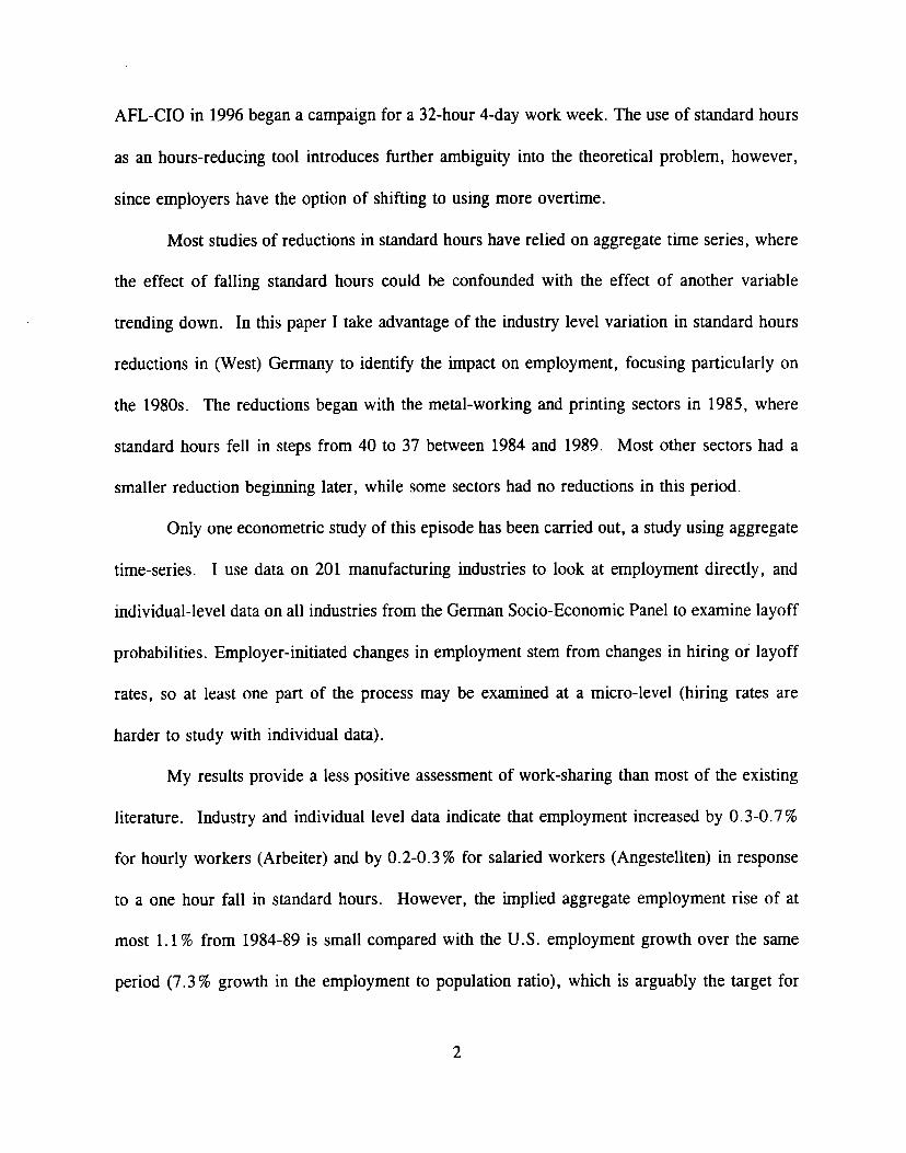
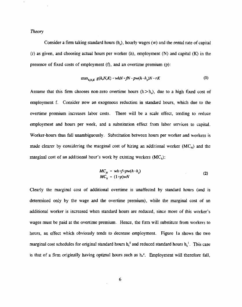
Consider a firm taking standard hours (h,), hourly wages (w) and the rental rate of capital

(r) as given, and choosing actual hours per worker (h), employment (N) and capital (K) in the

presence of fixed costs of employment (~, and an overtime premium (p):

‘h~~ g(hfl,fl - whN -P -pw(h -h,)N - rK (1)

Assume that this firm chooses non-zero overtime hours (h> ~), due to a high fixed cost of

employment f, Consider now an exogenous reduction in standard hours, which due to the

overtime premium increases labor costs. There will be a scale effect, tending to reduce

employment and hours per week, and a substitution effect from labor services to capital.

Worker-hours thus fall unambiguously. Substitution between hours per worker and workers is

made clearer by considering the marginal cost of hiring an additional worker (MC~) and the

marginal cost of an additional hour’s work by existing workers (MC~):

MC~ = wh+f+pw(h-h,)

MCh = (1 +p)wN(2)

Clearly the marginal cost of additional overtime is unaffected by standard hours (and is

determined only by the wage and the overtime premium), while the marginal cost of an

additional worker is increased when standard hours are reduced, since more of this worker’s

wages must be paid at the overtime premium. Hence, the firm will substitute from workers to

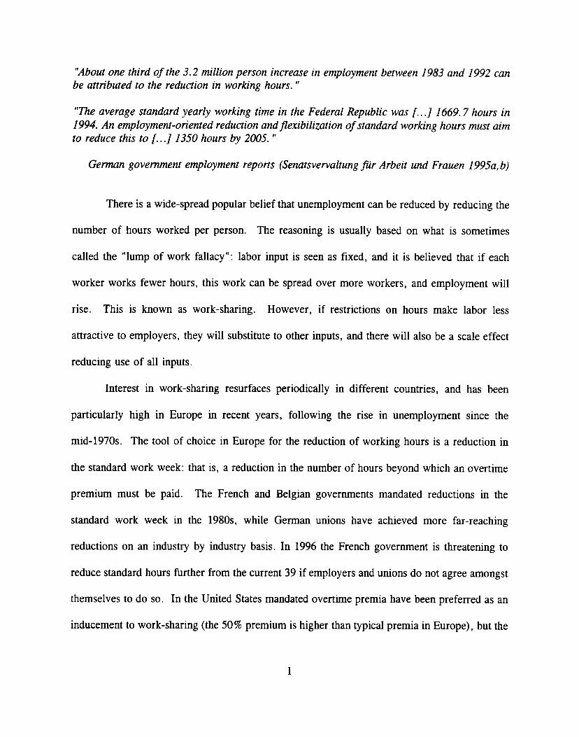
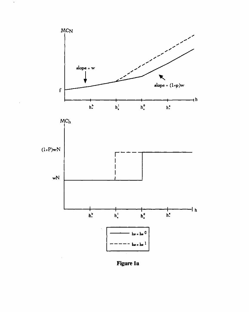
hours, an effect which obviously tends to decrease employment. Figure la shows the two

marginal cost schedules for original standard hours ho and reduced standard hours h,l. This case

is that of a firm originally having optimal hours such as h.’. Employment will therefore fall,

and the effect on weekly hours depends upon whether the scale effect and substitution from labor

to capital dominates the substitution from workers to hours.

Figure la makes clear, however, that the original optimal hours (and the magnitude of

the standard hours reduction) are critical for the response of the firm along the worker-hours

margin. Consider a firm whose optimal hours are below even the new standard hours, at h+b.

If we assume that the law constrains hours to be at least standard hours, this firm will move its

actual hours from the original kink point ~“ to the new kink point &l. MC~ has thus not

changed, while MC~ has fallen, and the firm will substitute from hours to workers, the opposite

of the previous case. The scale effect and the capital-labor substitution effect will work to

increase employment. The overall effect is that hours will fall, while employment will rise.

We could extend the analysis to cases permitting firms to work less than standard hours

(since this is possible in Germany, albeit not on a permanent basis). If a firm’s original hours

are below both the new and old standard, as

not affect its behavior. If its original hours

in htb in Figure la, the fall in standard hours will

are above the new standard hours, workers-hours

substitution will depend on all the magnitudes involved (while scale and capital-labor substitution

effects will tend to lower employment and hours).

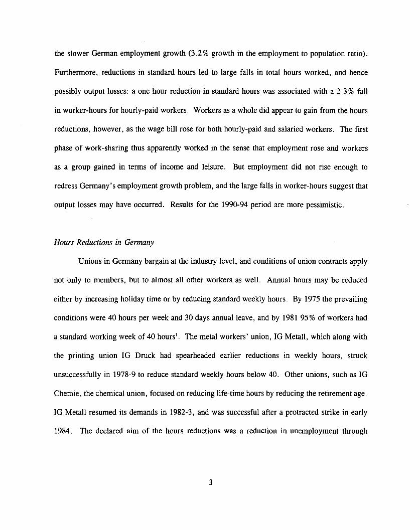
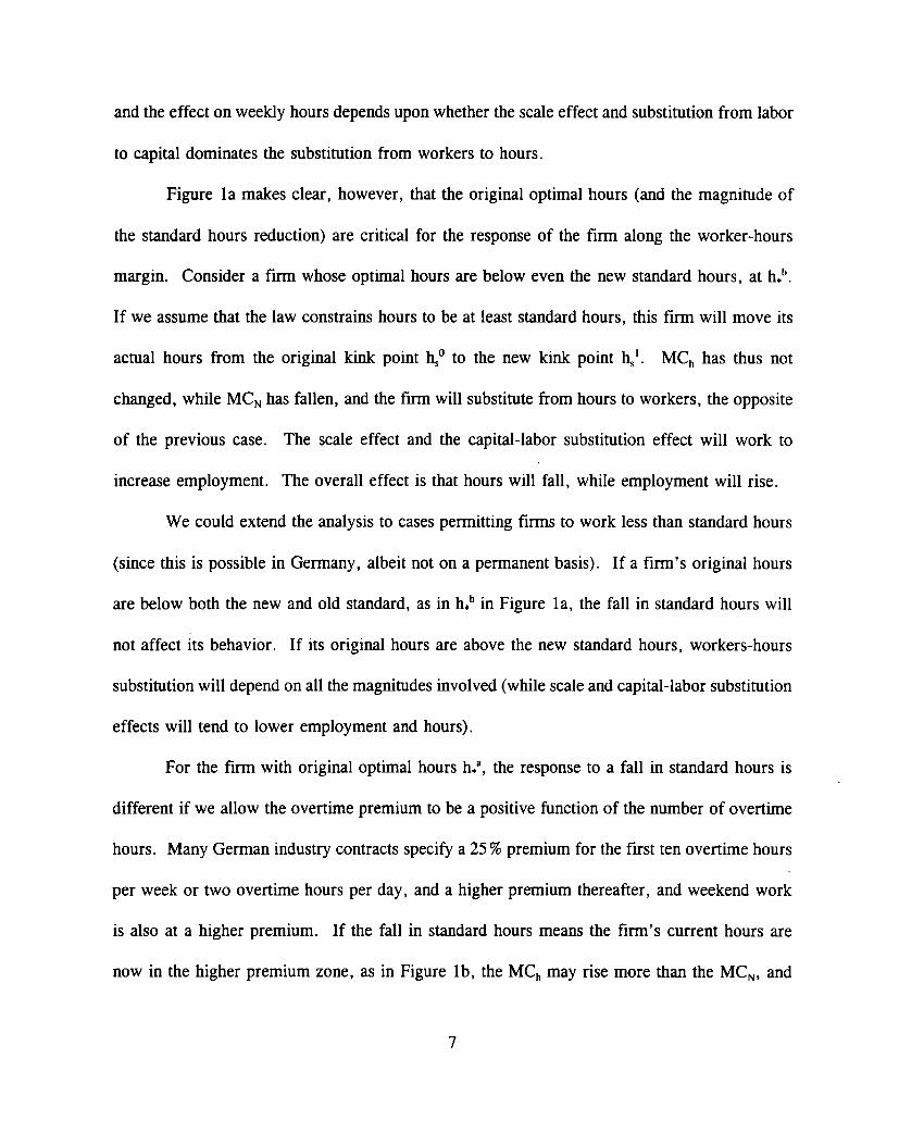
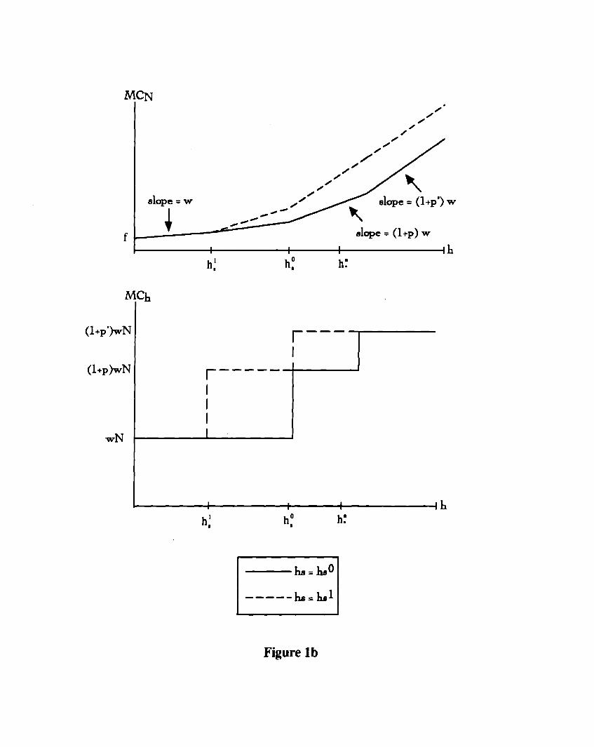
For the firm with original optimal hours h.’, the response to a fall in standard hours is

different if we allow the overtime premium to be a positive function of the number of overtime

hours. Many German industry contracts specify a 25 % premium for the first ten overtime hours

per week or two overtime hours per

is also at a higher premium. If the

day, and a higher premium thereafter, and weekend work

fall in standard hours means the firm’s current hours are

now in the higher premium zone, as in Figure lb, the MC~ may rise more than the MC~, and

7

the firm will substitute from hours to workers. The net effect on employment will be

ambiguous, and hours will fall.4

These cases make clear that if employment is to rise, there must be a large substitution

from hours to workers. The finding that actual hours fall a lot is a necessary condition for

work-sharing to be effective, but it is not a sufficient condition, since actual hours may be falling

due to the scale effect or substitution to capital.

It is important to consider that other parameters might change in response to the reduction

in standard hours. The overt concession in exchange for shorter standard hours on the part of

German unions was the introduction of greater flexibility. Presumably flexibility has a positive

scale effect, but it may be complementary with capital, and its effect on the trade-off between

workers and hours must be examined in a more complex model.

Another consideration important for Germany is that the hourly (straight-time) wage

apparently increased in response to standard hours deductions. A wage increase would cause

a substitution from hours to workers due to the fixed cost of hiring a worker. 5 The net effect

on hours per worker is therefore negative, and on employment is ambiguous, although we would

usually expect the scale effect and substitution to capital to predominate and lower employment,

Worker-hours will fall.6

Finally, it is possible that individuals are more productive when they work fewer hours.

Lower actual hours thus induce capital-saving technological progress. This has an ambiguous

effect on the already ambiguous employment response, but should lead to a larger fall (or lower

rise) in actual hours. Worker-hours still fall.

8

Previous Empirical Work

A number of papers use aggregate manufacturing times series data to look at the effect

of standard hours on actual hours per worker and employment, including Franz and Konig

(1986), who examine Germany from 1964-84, an earlier period of reduction in standard hours.

They report that a 1% reduction in standard hours raises employment by 1.09% and reduces

hours per worker by 0.99 %, which implies a slight rise in worker-hours. De Regt (1988) finds

an employment elasticity of -O.41 for the Netherlands in @e period 1954-82, and an hours per

worker elasticity of 0.89, implying a fall in worker-hours. Hart and Sharot (1978) find almost

identical results for UK males in the period 1961-72. Wadhwani (1987) and Faini and

Schiantarelli (1985) similarly estimate employment elasticities of -0.5, although they do not

estimate hours per worker elasticities. Brunello (1989), examining Japan in the period 1973-86,

finds a different result: that reducing standard hours has essentially no effect on actual hours,

although the employment elasticity is -0.34, thus implying a rise in worker-hours.

Hart (1987) uses pooled data for 25 German industries for 1969-81 and finds no response

of employment to standard hours, but that a 1% reduction in standard hours reduces hours per

worker (corrected for short time) by 1.2%. The variation in standard hours in this pooled

specification comes from both the cross-section and time-series. The only paper to examine

these issues using micro-data is Hart and Wilson (1988), which uses British firm-level data

pooled for the period 1978-82. They also find no response of employment to standard hours,

but find that a one hour reduction in standard hours reduces actual hours by 0.77 hours.

None of these papers describes the variation in standard hours that identifies the

coefficient of interest. With the time-series studies, standard hours may in many cases

9

essentially be a downward trend, and may proxy for omitted variables that are also falling over

time. Hart (1987) and Hart and Wilson (1988) use more suitable data, but the effect of pooling

time-series and cross-section observations is unclear - the use of a panel technique would have

been preferable.

Evidence on employment effects of the German standard hour reductions since 1984 is

not abundant. Using full-time workers in the GSOEP, Hunt (1996) finds that hours per worker

fell by 0.85-1 hour for each hour fall in standard hours. A necessary condition for employment

to rise is therefore satisfied. However, a second finding, that straight-time hourly wages rose

2-3 % for each hour reduction in standard hours, would work to reduce employment.

Stille and Zwiener (1987) attempt to tease out the effects of the 1985 standard hours

reduction in the metal-working sector by examining aggregate trends for that sector without

regression analysis. They judge that weekly overtime per person rose by half an hour due to

the standard hours reduction of 1.5 hours and that short time was unaffected by reductions in

standard hours, and influenced only by the business cycle. Their employment figures imply an

elasticity of employment with respect to standard hours of about -0.5, which lies between the

elasticities found by the employers’ association and the union. These results imply that worker-

hours stayed about the same. Finally, in the only econometric study of employment, Lehment

(1991) finds that when wage restraint is controlled for, reductions in standard hours are

insignificant in aggregate time series modelling employment growth for 1973-90.

10

Data

The principal data used are industry level data on manufacturing from the Statistisches

Bundesamt. Firms with at least twenty employees are required to report certain information to

the statistical office at the end of each month. The

belonging to these firms. The variables available are

data used here refer to establishments

employment and wage bills for hourly

workers (Arbeiter) and salaried

worked) for Arbeiter, and sales.

workers (Angestellten) separately,

Data are for 201 industries (a small

to problems with their data). Attention is focused on the first phase

1984 to 1989, although some results are presented for 1990-94

classification changes).

worker-hours (total hours

number were excluded due

of hours reductions from

(after 1994 the industry

‘Indices of collectively bargained wages (the average by industry for Arbeiter and

Angestellten) are available from the same source. However, these data are available only

quarterly, and have a different and more aggregated industry classification (45 categories), which

must be matched to that used for the rest of the data. Collectively bargained wages rather than

actual wages are used because the desired variable is the straight-time wage. Average actual

wages would include overtime pay, and hence confound wages and hours. Collectively

bargained wages are also slightly more exogenous to the firm, as there exists a certain amount

of wage drift (raising of wages above the collectively bargained floor).

Published standard hours by industry are obtained from tables supplied by the WSI

(Wirtschafts- und Sozialwissenschaftlichen Instituts des Deutschen Gewerkschaftbundes) (Hans-

Bockler-Stiftung 1995). In certain industries where standard hours vary by region, the average

across regions (weighted by employment) is computed.

11

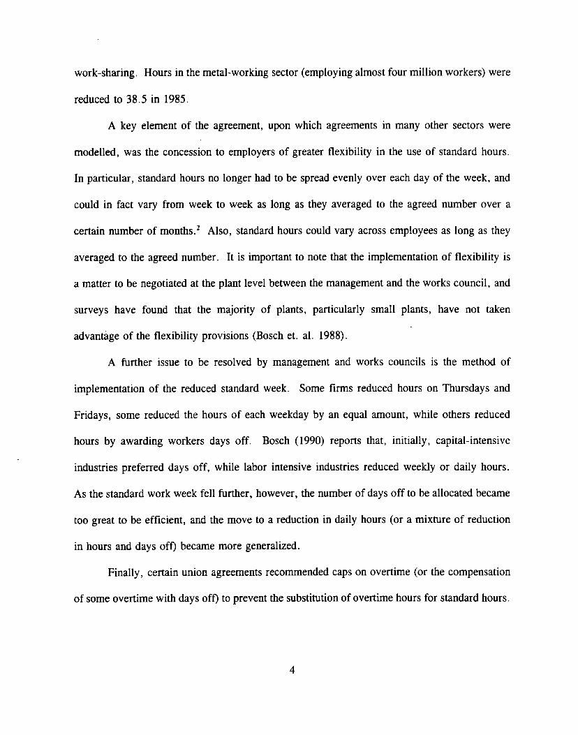
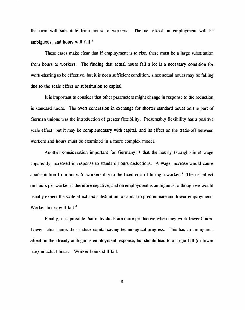
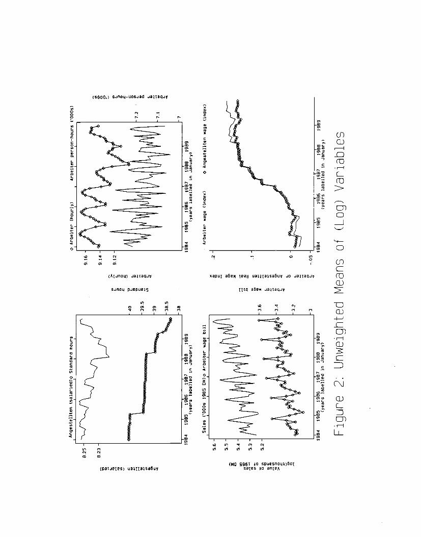
Figure 2 shows the means of the industry-level variables used.’ The means are

unweighed, which means that compared to aggregate patterns, small industries are

overrepresented. This appears to make average employment growth in the sample lower than

in the aggregate (although aggregate manufacturing employment did fall 1986-7). The spikes

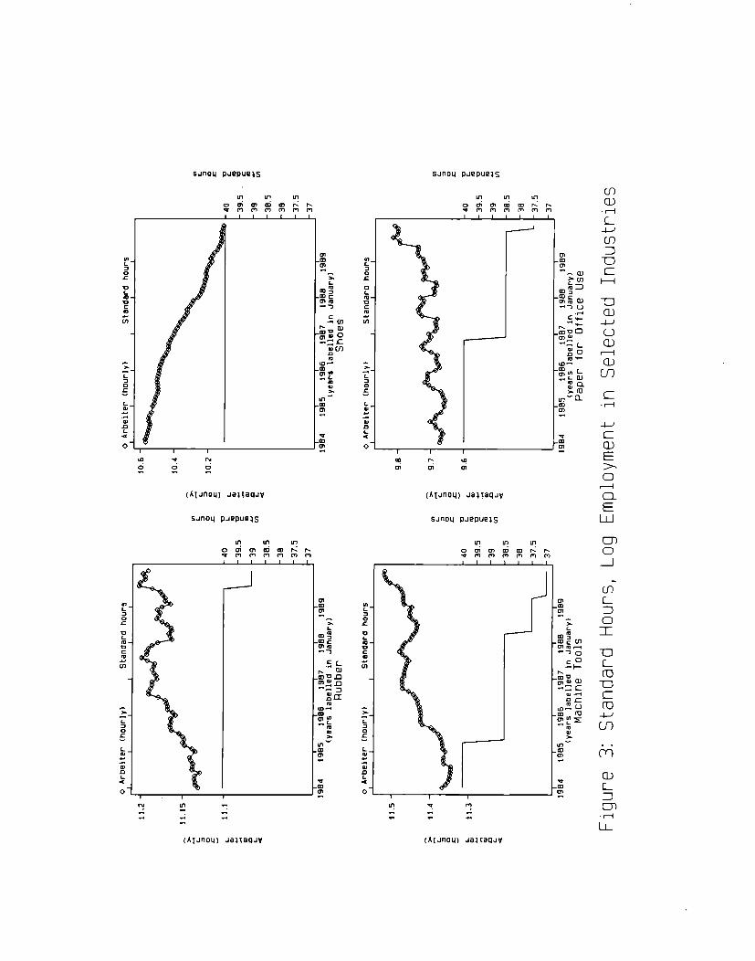
in the Arbeiter wage bill series are due to end of year bonuses. Figure 3 selects four industries

to represent the variety of standard hours reduction timing, and also plots employment of

Arbeiter (hourly workers).

Part of the analysis uses data from the German Socio-Economic Panel for the years 1984-

1989. In this section the standard hours variable is individual’s response to the question “What

are your collectively bargained weekly work hours without overtime?” (after the first survey,

the questionnaire specifies that if the respondent has more than one job, that s/he should refer

to the main job). The survey also asks respondents who are not working at the same job as in

the previous interview questions that seek to establish why the

used these responses to identify which job changes occurred

respondent changed jobs. I have

involuntarily (i. e. were fires or

layoffs). This is inherently somewhat subjective, relies on accurate reporting by respondents,

and assumes the quit/layoff distinction is meaningful. Therefore I also conduct analysis

assuming all separations are potentially involuntary.

When working with the individual data I focus on full-time workers (not possible in the

industry data), and hence drop respondents who said they had less than 35 standard hours. I

also drop workers who said their standard hours were greater than 45, to remove the most

obvious outliers (standard hours for all included industries were 40 or less throughout the sample

period). I drop workers in fishing, agriculture, or private households, and the self-employed,

12

for whom standard hours are not well-defined. I drop workers aged 550r over, since during

the period under consideration special agreements were reached insome industries to reduce the

hours ofolder workers below those ofothers in the same industry or to allow early retirement.

Ialsodrop those doing apprenticeships mdthoseunderage2O, although they could arguably

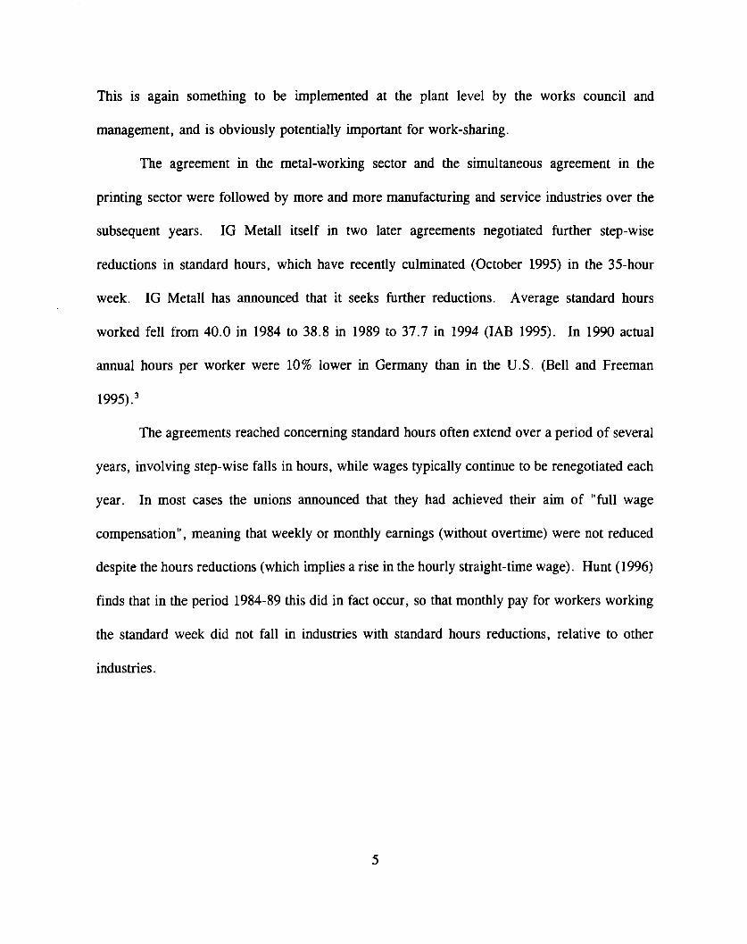
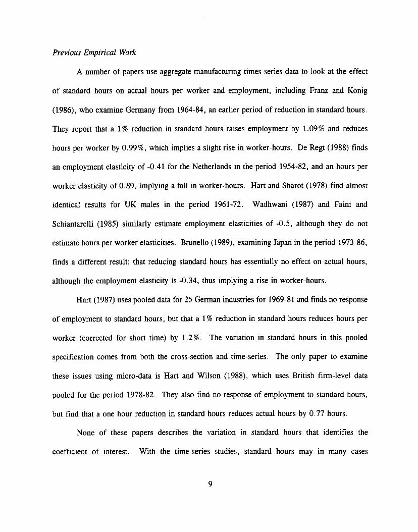
be included. Finally, I drop those with missing actual or standard (agreed) hours, industry, firm

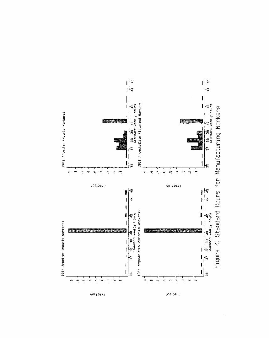
size, job type (self-employed, salaried etc), education, wage or job change information. Figure

4 shows the transformation in standard hours for 1984-89 as reported by manufacturing workers

in this sample.

Industry Level Results

The regressions using industry data are estimated using fixed effects. They include

month dummies interacted with dummies for ten aggregate industries to control for seasonal

patterns and are corrected for serial correlation of the errors with the iterative Cochrane-Orcutt

procedure. In addition to controlling for standard hours in the regressions, I control for sales

in each industry. This may be viewed as controlling for demand or, since sales and output are

closely related, for the scale effect. Including sales should control for endogeneity of

introduction of lower standard hours: if employers in industries expecting booms conceded lower

standard hours, this could lead to a negative sign on standard hours in an employment regression

(although a priori the endogeneity could go the other way). Thus specifications controlling for

sales should be free of bias due to endogenous hours reductions, unless industries introducing

lower standard hours were those expecting the capital to labor ratio to change in a particular

13

direction, which does not seem compelling. Notice that if the more flexible use of hours caused

a positive scale effect, this too will be controlled for.

Results will be presented both controlling for wages and omitting wages. Some

component of changes in wages is part of the German work-sharing experiment, and the

coefficient on standard hours with wages omitted is of interest. The counterfactual of unchanged

wages is also of some interest, however, to get an idea of what might happen when standard

hours are reduced in an institutional setting where wages might behave differently. *

Table 1 presents results of regressions omitting wages. The dependent variable of the

first column is the log of Arbeiter (hourly-paid workers) at the end of the month. The

coefficient on standard hours is negative and significant, with a magnitude indicating that a one

hour reduction in standard hours would increase employment by 0.3 %. If confidence is placed

in the theoretical prediction of a negative scale effect, and controlling for sales controls for the

scale effect, then this result is an upper bound on the beneficial impact on employment of

standard hours reductions. The net effect may even have been negative. Increased flexibility of

hours could play a role, but

Flexibility presumably does

is urdikely to be introducing a bias towards pessimistic results.

not cause substitution away from labor services; the effect on

substitution between hours per worker and workers is unclear, but it is unlikely that flexibility

reduced substitution from hours per worker substantially, since we shall see below that this

substitution seems to be close to its theoretical maximum.

The second column examines the effect of standard hours on the total hours worked by

Arbeiter over the month (worker-hours). The coefficient on standard hours is large and positive,

indicating that a one hour reduction in standard hours reduced worker-hours by 2,1%. If the

14

coefficient is also picking up substitution toward labor services due to increased hours flexibility,

the fall due to standard hours reductions alone would be more than 2.1%.

The third column uses the ratio of worker-hours and workers to construct hours per

worker (for Arbeiter), in order to see whether the effect of standard hours appears to be the

same in the industry data as in the individual data of Hunt (1996). The coefficient suggests that

a one hour fall in standard hours reduced hours per worker by 2.5%. The individual level result

of Hunt (1996) was that a full-time worker’s typical work week fell by 0.85-1 hour when

standard hours fell one hour, or a 2.1-2.4 % fall. The industry and individual data are thus fairly

consistent. The coefficients on standard hours are fairly consistent across the three measures of

Arbeiter labor inputs: a reduction of 2.5% in hours per worker (column 3) coupled with a rise

of 0.3 % in employment (column 1) implies a reduction in worker-hours of about 2.2%, close

to the 2.1% estimated in column 2.

No data on worker-hours for Angestellten (salaried workers) are available, but the

dependent variable of the fourth column is the log of Angestellten employed at the end of the

month. The coefficient on standard hours suggests that reducing standard hours by one hour

raised employment of Angestellten by 0.2 %, similar to the effect found for Arbeiter. The

individual level data used in Hunt (1996) suggested that actual hours for Angestellten fell about

one for one with standard hours, although these results were not as reliable as those for Arbeiter

(Hunt 1996). Together with the results of column 4 this implies a large fall in Angestellten

worker-hours, as for Arbeiter.

Thus for both Arbeiter and Angestellten, employment may have risen in response to a

one hour reduction in standard hours, by 0.2-0.3 %, implying an elasticity of about -0.06 to

15

-0.10. This is on the low end of the range found by the existing literature. This employment

rise had a considerable cost in terms of lost worker-hours, which fell by 2.1% in response to

a one hour standard hour reduction, an elasticity of 0.84.

However, since hourly wages are known from the results of Hunt (1996) to have risen

when standard hours fell, the impact on the wage bill will be much less than on worker-hours,

and could even be positive. If the wage bill rises, the group of workers that decided to reduce

standard hours will be better off as a group even if some of them lose their job, and if

redistribution occurred (for example through the union) each member of the group could be

better off. Unions are sometimes modelled as wage-bill maximizers. Columns 5 and 6 examine

the influence of standard hours on the wage bills of Arbeiter and Angestellten, and the

coefficients on standard hours are negative and significant. The rises of 2.7 % (for Arbeiter) and

3.9 % (for Angestellten) associated with a one hour reduction in standard hours seem large in

light of the results of Hunt (1996), which found that straight-time hourly wages rose 2-3%.

Table 2 adds the indices of collectively bargained wages for Arbeiter and Angestellten

to the regressions of Table 1, The coefficients on the added variables do not always have the

expected signs: in particular, the coefficients on the two wage variables are essentially the same

in the Arbeiter regression as in the Angestellten regression. It is thus not entirely clear what is

being captured by the wage variables. The coefficients on standard hours are less significant

than in Table 1, but generally paint a less optimistic picture. This is unexpected, since

controlling for what is thought to be a wage rise should make standard hours reductions look

better for employment. The coefficient for Angestellten changes sign to become significant and

positive, indicating that reducing standard hours by one hour reduced employment by 0.2%.

16

Thesign changes for Arbeiter too, although thecoefficient is insignificant. The coefficient in

the regression for worker-hours becomes small and insignificant (this change is in the expected

direction). Finally, the coefficient on hours per worker falls. The results for worker-hours and

hours per worker could have the interpretation that some of their fall in response to reductions

in standard hours was in fact due to the accompanying wage rise.

Table

average level

3 presents the results of weighted regressions. Regressions are weighted by the

of the dependent variable, with the exception of the hours per worker regression,

which is weighted by average number of Arbeiter. The weighted regressions have the advantage

that means are close to the means across workers. However, if the correct unit of analysis is

in fact the firm, and aggregation has uncertain effects, it may not be an improvement to down-

weight observations on small industries. Weighting increases the contribution to the estimates

of the large industries that struck in 1984 under IG Metall, and therefore provides an indication

as to whether the strike could be influencing the results.

The results are qualitatively similar to the unweighed results, although the magnitudes

of the standard hours coefficients differ, especially for Arbeiter worker-hours and the wage bills,

where the coefficients are considerably smaller and larger, respectively. The results of this table

suggest that a one hour fall in standard hours leads to

Angestellten and a 0.14 % rise in employment of Arbeiter.

The regressions presented so far have not taken into

a 0.26 % rise in employment of

account the fact that in some cases

firms might anticipate reductions in standard hours, since these were often known in advance,

nor that, particularly in cases where reductions took effect immediately they were agreed, the

firms might need some time to respond. The regressions of Table 4 add to the regressors six

17

leads and six lags of standard hours, and the sum of all the standard hours coefficients,

representing the steady-state effect, is reported. The results of these (unweighed) regressions

are similar to the regressions of Table 1 including only current standard hours, although the

standard hours “coefficient” is larger, most notably for the Arbeiter regression. Hence a one

hour reduction in standard hours is associated with a 2.7 % fall in Arbeiter worker-hours, a 0.7 %

rise in Arbeiter employment, and a 0.3 % rise in Angestellten employment. The implied

elasticity for Arbeiter, -0.26, is still lower than those estimated in the time-series literature.

These results and those of Table 1 are preferred to the specifications including wages or using

weighting.

A final set of results based on data for 1990-1994 is presented in Table 5. This period

is not as good for the purposes of this study, since a widespread move to begin cutting hours

between mid- 1989 and mid- 1990 means that all industries have falling standard hours. The

effect of interest is thus identified from differing rates of the fall in standard hours. Also, the

last years of the data seem to be of poorer quality, and 8% of the observations are missing for

the period 1990-1994. Table 5 does not provide evidence that cuts in standard hours increase

employment, g

The specification that has shown the most beneficial effects of standard hours reductions

is the coefficient of -0.0066 in the Arbeiter equation using leads and lags (column 1 of Table

4). Average standard hours in the sample fell 1.7 hours from 1984 to 1989, so this coefficient

implies a 1.1% employment gain due to work-sharing. Compared to the growth in

manufacturing employment of 5.2% from 1984-89 this is significant, although not large.

However, perhaps a better comparison is with the level of employment growth that was hoped

18

for over this period. Employment in the U.S. grew 11.6% and the employment to population

ratio grew 7.3 % (compared to 3.2% in Germany). Clearly, the employment growth achieved

in Germany through work-sharing is not close to bridging the German-American employment

growth gap. Furthermore, the large associated reductions in worker-hours suggest that the

standard hours reductions introduced a serious distortion and may have resulted in considerable

output loss .

Individual Level Results

Table 6 presents results from the GSOEP on the probability of a worker separating

involuntarily from the current job. A fixed effects conditional logit specification is used. The

regressors include year dummies, the current wage, current standard hours (as reported by the

respondent), and expected standard hours for the following year, to allow workers to anticipate

announced changes. Expected standard hours are calculated by averaging

responses in the following year of those in the individual’s current industry

the standard hours

and job type. The

results are similar (i. e. the coefficient is also insignificant) if expected standard hours are based

on published sources. Industry dummies are not generally included as, surprisingly, the

hypothesis that their coefficients were jointly zero could only be rejected in one regression.

Arbeiter in services and Angestellten in manufacturing are not broken out separately, as too few

separations identify the coefficients of interest. Manufacturing for the individual data does not

include construction, for consistency with the industry data.

For Arbeiter in all industries grouped together, the coefficient on standard hours is

positive and significant, suggesting a 7% decline in the probability of involuntary separation. 10

19

Since theprobability ofaninvoluntary separation is 4.2% for this group, aone hour reduction

in standard hours would reduce this probability to 3.8%, raising employment by about 0.3 %

(ignoring any effect on hires, of course). This falls within the range found using industry data.

If the effect on hires is of a similar magnitude, the total effect would be similar to the largest

effect found with industry data. For other groups the coefficient on standard hours is

insignificant, except when the whole sample is used. The similarity of the coefficients for

Arbeiter in manufacturing, all Arbeiter, and the whole sample suggests that reducing standard

hours has similar employment effects in services and manufacturing.

Expected standard hours always has an insignificant coefficient. Insofar as the coefficient

for Arbeiter in manufacturing is insignificant, these results do not accord with the industry level

data for manufacturing. Even for this group, the number of separations that identi~ the

coefficient is not large, however. Notice that the wage variable has a negative sign, and is

hence probably capturing information about how the firm values the individual, rather than a

labor demand story about how the firm responds to exogenous union wage increases.

If the regressions are rerun with the probability of any type of separation as the

dependent variable, the results are similar in terms of significance, but coefficients are smaller.

Conclusions

Using manufacturing data on 201 detailed industries for 1984-89, I find that reductions

in standard hours were associated with rises in employment. I find that, in the preferred

specifications, a one hour fall in standard hours raised employment of hourly workers (Arbeiter)

by 0,3-0. 7% and employment of salaried workers (Angestellten) by 0.2-0.3%. However, I find

20

that worker-hours

in standard hours.

of hourly workers (Arbeiter) fell by 2-3% in response to a one hour reduction

These results are conditional on sales, which removes endogeneity associated

with the adoption of lower standard hours, but may to some extent control for the scale effect,

expected to be negative. Hence, the employment rises may be upper bounds and the worker-

hours fall a lower bound. The implied elasticities for employment are at the low end of the

range in the existing literature on work-sharing, and the implied growth in employment of at

most 1.1 % (in response to a 1.7 hour reduction in mean standard hours) is small compared with

growth in U.S. employment over the same period.

Due to a rise in straight-time hourly wages, the wage bill actually rose in conjunction

with reduced standard hours, despite reduced worker-hours, for both Arbeiter and Angestellten.

This indicates that workers as a group benefited from hours reductions.

The employment results from industry level data are supported by analysis of the

probability of an involuntary separation in the individual level Socio-Economic Panel data, For

Arbeiter in manufacturing and services together a one hour reduction in standard hours reduced

the probability of an involuntary separation by 7%, a magnitude which would imply an

employment rise of 0.3 %, similar to the industry-level results. For Angestellten standard hours

had no significant effect on separations.

Industry-level results for the period

employment fell when standard hours fell.

1990-1994 are more pessimistic, and suggest that

Although this period, when standard hours were

falling in all industries, is less suitable for study, these results do caution that employment

outcomes could be different in different economic environments.

21

The good news from the first phase of Germany’s work-sharing experiment is thus that

employment rose, and that the wage bill increased. The bad news is that employment did not

rise enough to bring the German employment growth rate close to the American rate, and the

large fall in worker-hours indicates that an important distortion was introduced, which may have

caused loss of output.

22

References

Bell, Linda and Richard Freeman. 1995. “Why Do Americans and Germans Work DifferentHours?”. In Friedrich Buttler et. al. eds. Institutional Frameworks and Lubor MarketPe@onnance: Comparative views on the U.S. and Gewn Economies Ruttledge, NewYork.

Booth, Alison and Martin Ravallion. 1993. “Employment and Length of the Working Week ina Unionized Economy in which Hours of Work Influence Productivity. ” EconomicRecord pp.428-436.

Booth, Alison and Fabio Schiantarelli. 1987. “The Employment Effects of a Shorter WorkingWeek”. Economics pp. 237-248.

Bosch, Gerhard. 1990. “From 40 to 35 hours: Reduction and flexibilisation of the working weekin the Federal Republic of Germany”. International Labour Review pp.61 1-627.

Bosch, Gerhard et. al. 1988. Arbeitszeitverkiirzung im Betrieb: Die Umsetzung der 38. 5-Stunden-Woche in der Metall-, Druck- und Holzindustrie sowie im Einzelhandel K61n.

Bosch, Gerhard and Steffen Lehndorff. (n.d.) “Annual Working Hours in Germany”. Institut firArbeit und Technik mimeo.

Brunello, Giorgio. 1989. “The Employment Effects of Shorter Working Hours: An Applicationto Japanese Data. ” Economics pp. 473-86.

Calmfors, Lars. 1985. “Work Sharing, Employment and Wages. ” European Economic Reviewpp.293-309 .

deRegt, Erik. 1988. “Labor Demand and Standard Working Time in Dutch Manufacturing,1954- 1982.” In Robert Hart ed. Employment, Unemployment and Labor UtilizationUnwin Hyman, Boston.

Earle, John, and John Pencavel. 1990. “Hours of Work and Trade Unionism”. Journal of LaborEconomics pp. S150-174.

European Industrial Relations Review various issues.

Faini, Riccardo and Fabio Schiantarelli. 1985. “A Unified Frame for Firms’ Decisions:Theoretical Analysis and Empirical Application to Italy, 1970-1980.” In Daniel Weiserbs,ed., International Studies in Economics and Econometrics. Amsterdam: Martinus Nijhoff.

23

Franz, Wolfgang and Heinz Konig. 1986. “The Nature and Causes of Unemployment in theFederal Republic of Germany since the 1970s: An Empirical Investigation, ” Economicspp. S219-S244.

Freeman, Richard. 1995. “Work-Sharing to Full Employment: Serious Option or PopulistFallacy?”. Harvard University mimeo.

Hamermesh, Daniel. 1993. L.ubor Demnd. Princeton University Press.

Hamermesh, Daniel. 1995. “The Demand for Workers, Hours and Days”. Universi~ of Texasmimeo.

Hans-Bockler-Stiftung des Deutschen Gewerkschaftbundes. 1995. WSI-Informutionen zur

Hart,

Hart,

Hart,

Heel,

Tarifiolitik: A;beitszeitkalendar West und Ost 1995. Diisseldorf.

Robert. 1987. Working Time and Employment Allen and Unwin, Boston.

Robert and T Sharot. 1978. “The Short-Run Demand for Workers and Hours: A RecursiveModel. ” Review of Economic Studies pp.299-309.

Robert and Nicholas Wilson. 1988. “The Demand for Workers and Hours: MicroEvidence from the UK Metal Working Industry. ” In Robert Hart ed. Employment,Unemployment and kbor Utilization

Michael. 1987. “Can Shorter WorkingUnemployment and tibor Utilization

Unwin Hyman, Boston.

Time Reduce Unemployment?” In C .H Siven, ed.Unwin Hyman, Boston.

Houpis, George. 1993. “The Effect of Lower Hours of Work on Wages and Employment. ”

Hunt,

Hunt,

Centre for Economic Performance, LSE, mimeo.

Jennifer. 1995. “Which Slows Employment Adjustment More: Firing Costs orRestrictions on Hours Per Worker?”, Yale University mimeo.

Jemifer. 1996. “The Response of Wages and Actual Hours Worked toStandard Hours in Germany.” Hoover Institution mimeo.

Institut fir Arbeitsmarkt- und Berufsforschung (IAB). Various tables.

Konig, Heinz and Winfried Pohlmeier. 1988. “A Dynamic Model of LaborRobert Hart ed. Employment, Unemployment and Lubor UtilizationBoston.

the Reduction of

Utilization, ” InUnwin Hyman,

24

Lehment, Harmen. 1991, ''LohnuficMal~ng, Arbeitszeitvertirzung und Beschafiigung. Eineempirische Untersuching fir die Bundesrepublik Deutschland 1973-1990.” DieWeltwirtschafi pp,72-85.

Senatsverwaltung fir Arbeit und Frauen - Beirat Arbeitsmarktpolitik. 1995a. Berliner Erklarung- Zur Halbiewng der Arbeitslosigkeit bis zum Jahr 2000 Berlin.

Senatsverwaltung fi.ir Arbeit und Frauen - Beirat Arbeitsmarktpolitik. 1995b. BerlinerMemorandum zur Arbeitszeitpolitik 2000 Berlin.

Stille, Frank and Rudolf Zwiener. 1987. “Beschaftigungswirkungen der Arbeitszeitverfirzungvon 1985 in der Metallindustrie. ” Deutsches Institut fir WitischafisforschungWochenbericht pp. 273-279.

Wadhwani, Sushil. 1987. “The Effects of Inflation and Real Wages on Employment. ”Economics pp.21-40.

WSI-Mitteilungen Zeitschrift des Wirtschafts- und Sozialwissenschaftlichen Instituts desDeutschen Gewerkschaftbundes GmbH. Various issues, Bund Verlag, Koln.

25

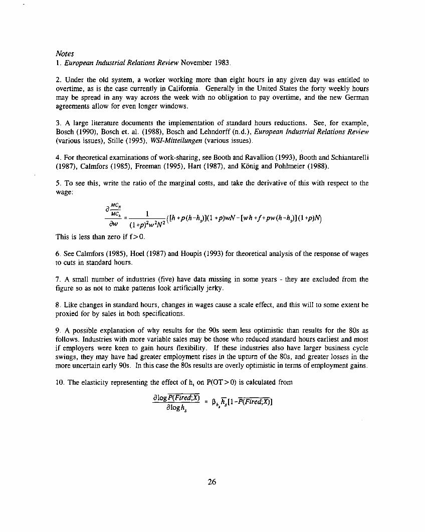
Notes1. European Industrial Relations Review November 1983.

2. Under the old system, a worker working more than eight hours in any given day was entitled toovertime, as is the case currently in California. Generally in the United States the forty weekly hoursmay be spread in any way across the week with no obligation to pay overtime, and the new Germanagreements allow for even longer windows.

3. A large literature documents the implementation of standard hours reductions. See, for example,Bosch (1990), Bosch et. al. (1988), Bosch and Lehndorff (n.d.), European Industrial Relations Review(various issues), Stille (1995), WSI-A4itleilungen (various issues).

4. For theoretical examinations of work-sharing, see Booth and Ravallion (1993), Booth and Schiantarelli(1987), Calmfors (1985), Freeman (1995), Hart (1987), and Konig and Pohlmeier (1988).

5. To see this, write the ratio of the marginal costs, and take the derivative of this with respect to thewage:

MCNa—“h - 1— -* (1+p)2w2N2

([h +p(h-h,)](l +p)wN- [Wh+f+pw(h-h.)l(l+p)q

This is less than zero if f >0.

6. See Calmfors (1985), Heel (1987) and Houpis (1993) for theoretical analysis of the response of wagesto cuts in standard hours.

7. A small number of industries (five) have data missing in some years - they are excluded from thefigure so as not to make patterns look artificially jerky.

8. Like changes in standard hours, changes in wages cause a scale effect, and this will to some extent beproxied for by sales in both specifications.

9. A possible explanation of why results for the 90s seem less optimistic than results for the 80s asfollows. Industries with more variable sales may be those who reduced standard hours earliest and mostif employers were keen to gain hours flexibility. If these industries also have larger business cycleswings, they may have had greater employment rises in the upturn of the 80s, and greater losses in themore uncertain early 90s. In this case the 80s results are overly optimistic

10. The elasticity representing the effect of h, on P(OT > O) is calculated

in terms of employment gains.

from

dlogP(Fire~~

alogh,= ~~,~[1 -P(Fire~X)]

26

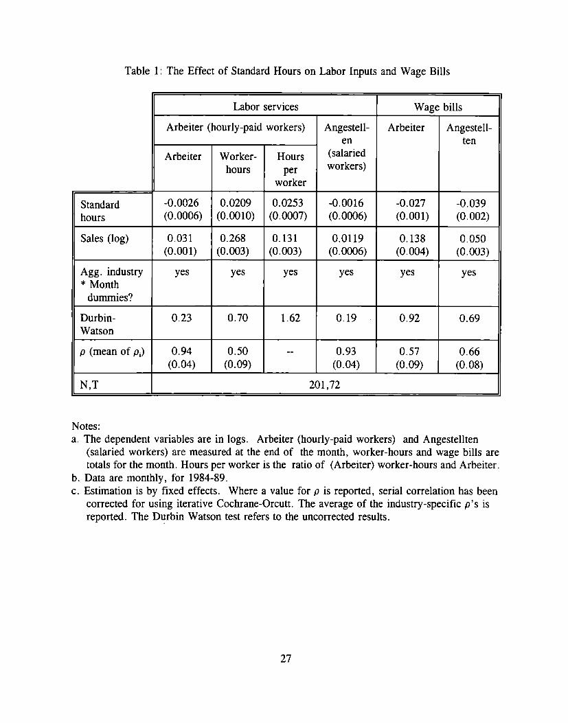
Table 1: The Effect of Standard Hours on Labor Inputs and Wage Bills

Standardhours

Sales (log)

Agg. industry* Month

durnrnies?

Durbin-Watson

p (mean of Pi)

N,T

Notes:a.

b.c.

Labor services

Arbeiter (hourly-paid workers)

worker

-0.0026 0.0209 0.0253(0.0006) (0.0010) (0.0007)

0.031 0.268 0.131(0.001) (0.003) (0.003)

yes yes yes

0.23 0,70 1.62

0.94 0.50 --(0.04) (0.09)

Angestell-

(sa;~iedworkers)

-0,0016(0.0006)

0.0119(0.0006)

yes

0.19

0.93(0.04)

201,72

Wage bills

Arbeiter

-0.027(0.001)

0.138(0.004)

yes

0.92

0.57(0.09)

Angestell-ten

-0.039(0.002)

0.050(0.003)

yes

0.69

0.66(0.08)

The dependent variables are in logs. Arbeiter (hourly-paid workers) and Angestellten(salaried workers) are measured at the end of the month, worker-hours and wage bills aretotals for the month. Hours per worker is the ratio of (Arbeiter) worker-hours and Arbeiter.Data are monthly, for 1984-89.Estimation is by fixed effects. Where a value for P is reported, serial correlation has beencorrected for using iterative Cochrane-Orcutt. The average of the industry-specific p‘s isreported. The Durbin Watson test refers to the uncorrected results.

27

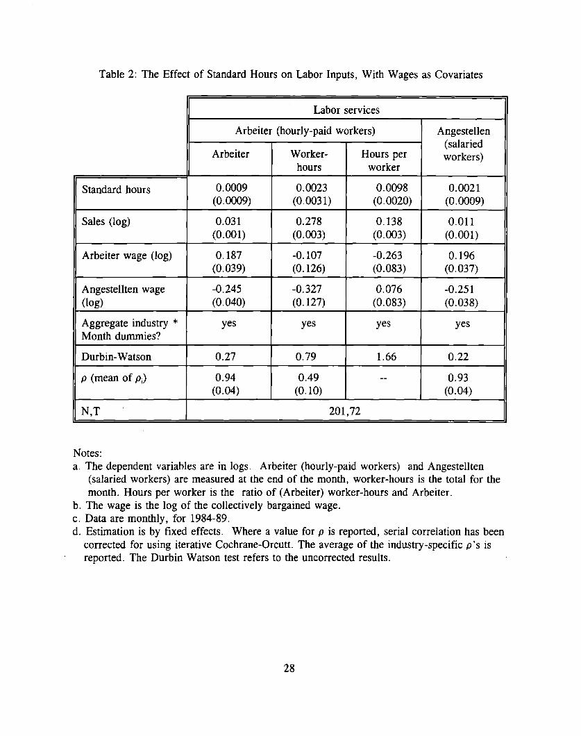
Table 2: The Effect of Standard Hours on Labor Inputs, With Wages as Covariates

II Labor services

Arbeiter (hourly-paid workers) Angestellen(salaried

Arbeiter Worker- Hours per workers)hours worker

Standud hours 0.0009 0.0023 0.0098 0.0021(0.0009) (0.0031) (0.0020) (0.0009)

Sales (log) 0.031 0.278 0.138 0.011(0.001) (0.003) (0.003) (0.001)

Arbeiter wage (log) 0.187 -0.107 -0.263 0.196(0.039) (O.126) (0.083) (0.037)

Angestellten wage -0.245 -0.327 0.076 -0.251(log) (0.040) (O.127) (0.083) (0.038)

Aggregate industry * yesI

yes yes yesMonth dummies?

Durbin- Watson I 0.27 I 0.79 I 1.66 I 0.22

p (mean Of pi) 0.94 0.49 -- 0.93(0.04) (0. 10) (0.04)

N,T I 201,72

Notes:a. The dependent variables are in logs. Arbeiter (hourly-paid workers) and Angestellten

(salaried workers) are measured at the end of the month, worker-hours is the total formonth. Hours per worker is the ratio of (Arbeiter) worker-hours and Arbeiter.

b. The wage is the log of the collectively bargained wage.c. Data are monthly, for 1984-89.

the

d. Estimation is by fixed effects. Where a value for p is reported, serial correlation has beencorrected for using iterative Cochrane-Orcutt. The average of the industry-specific p‘s isreported. The Durbin Watson test refers to the uncorrected results.

28

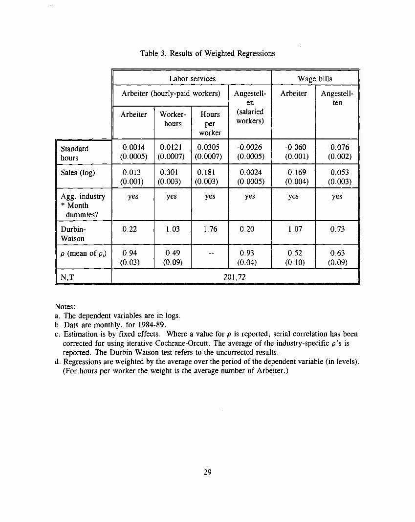
Table 3: Results of Weighted Regressions

Labor services Wage bills

Arbeiter (hourly-paid

,=Aworkers)

Hoursper

worker

Angestell-

(sa~iedworkers)

Angestel,ten

Arbeiter

0.0305 -0.0026(0.0007) (0.0005)

Standard -0.0014 0.0121

hours (0.0005) (0.0007)-0.060(0.001)

-0.076(0.002)

Sales (log) 0.013 0.301(0.001) (0.003)

0.181 0.0024(0.003) (0.0005)

0.169(0.004)

0.053(0.003)

Agg. indust~ yes yes* Month

dummies?

yes yes yes yes

E1.76 0.20

-- 0.93(0.04)

201,72

Durbin- 0.22 1,03Watson

1.07 0.73

p (mean Of pi) 0.94 0.49(0.03) (0.09)

0.52(o. 10)

0.63(0.09)

N,T I

Notes:a. The dependent variables are in logs.b. Data are monthly, for 1984-89.c. Estimation is by fixed effects. Where a value for P is reported, serial correlation has been

corrected for using iterative Cochrane-Orcutt. The average of the industry-specific p‘s isreported. The Durbin Watson test refers to the uncorrected results.

d. Regressions are weighted by the average over the period of the dependent variable (in levels).(For hours per worker the weight is the average number of Arbeiter.)

29

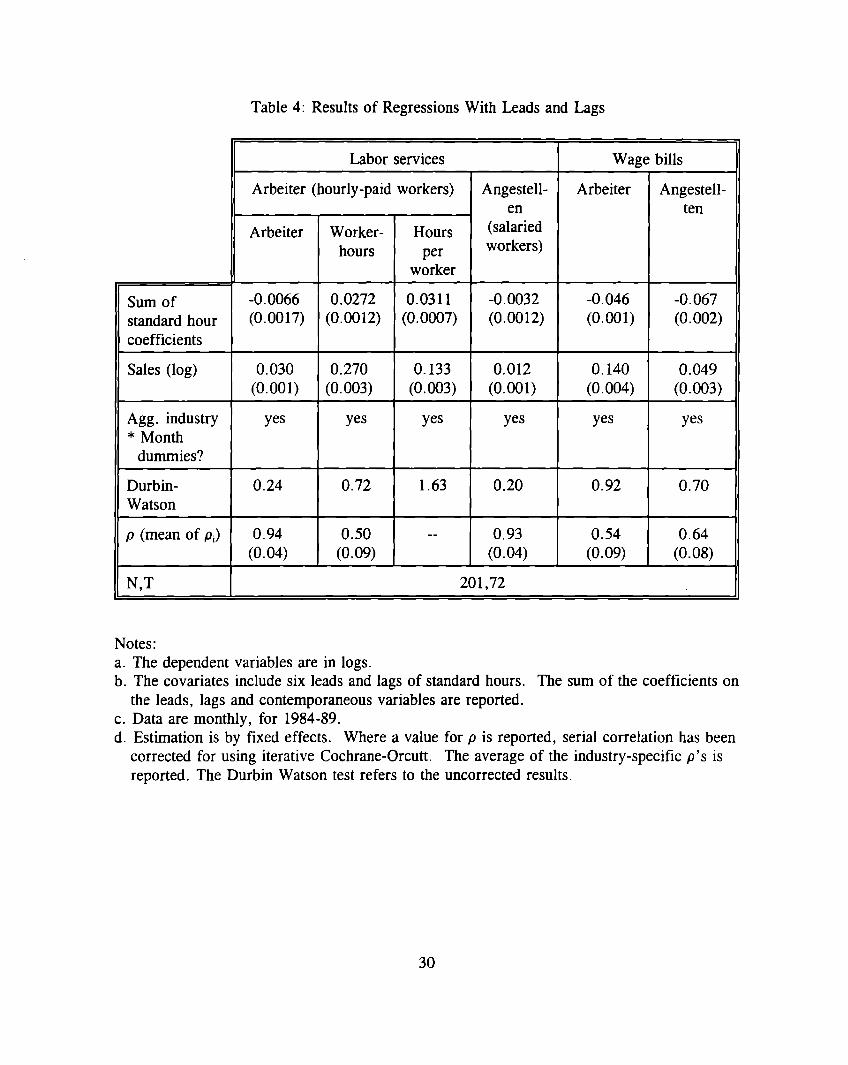
Table 4: Results of Regressions With Leads and Lags

Labor services

Arbeiter (hourly-paid workers)

Arbeiter

Sum of -0.0066

standard hour (0.0017)

coefficients

Sales (log) 0.030(0.001)

Agg. industry yes* Month

dummies?

Durbin- 0.24Watson

a.b.

c.d.

Worker- Hourshours per

worker

Angestell-

(sa;~iedworkers)

0.0272 0.0311 -0.0032(0.0012) (0.0007) (0.0012)

0.270 0.133 0.012(0.003) (0.003) (0.001)

yes yes yes

0.72 1.63 0.20

0.50 -- 0,93(0.09) (0.04)

201,72

Wage bills

Arbeiter

-0.046(0.001)

0.140(0.004)

yes

0.92

0.54(0.09)

Angestell-ten

-0.067(0.002)

0.049(0.003)

yes

0.70

0.64(0.08)

Notes:The dependent variables are in logs.The covariates include six leads and lags of standard hours. The sum of the coefficients onthe leads, lags and contemporaneous variables are reported.Data are monthly, for 1984-89.Estimation is by fixed effects. Where a value for p is reported, serial correlation has beencorrected for using iterative Cochrane-Orcutt. The average of the industry-specific p‘s isreported. The Durbin Watson test refers to the uncorrected results.

30

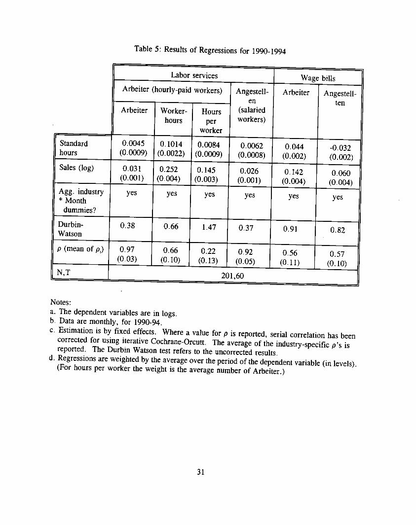
Table 5: Results of Regressions for 1990-1994

Labor services Wage bills

Arbeiter (hourly-paid workers) Angestell- Arbeiter Angestell-ten

Arbeiter Worker- Hours (sa~ried

hours per workers)

worker

Standard 0.0045 0.1014 0.0084 0.0062 0,044hours

-0.032(0.0009) (0.0022) (0.0009) (0.0008) (0.002) (0.002)

Sales (log) 0.031 0.252 0.145 0.026 0.142 0.060(0.001) (0.004) (0.003) (0.001) (0.004) (0.004)

Agg. industry yes yes yes* Month

yes yes yes

dummies?

Durbin- 0.38 0.66 1.47 0.37 0,91 0.82Watson

p (mean of pi) 0.97 0.66 0.22 0.92(0.03)

0.56(0. 10)

0.57(0. 13) (0.05) (0.11) (o. 10)

N,T 201,60

Notes:a. The dependent variables are in logs.b. Data are monthly, for 1990-94.c. Estimation is by fixed effects. Where a value for p is reported, serial correlation has been

corrected for using iterative Cochrane-Orcuti. The average of the industry-specific p‘s isreported. The Durbin Watson test refers to the uncorrected results.

d. Regressions are weighted by the average over the period of the dependent variable (in levels).(For hours per worker the weight is the average number of Arbeiter.)

31

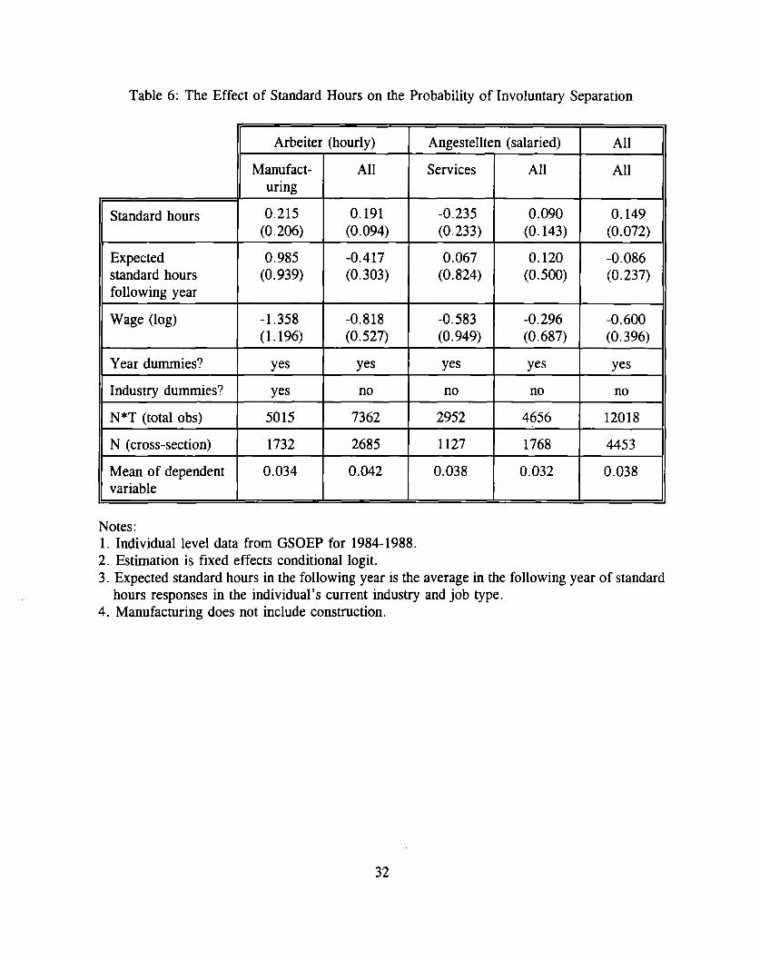
Table6: The Effect of Shndard Hours ontie Probability of Involunt~ Separation

Arbeiter (hourly) Angestellten (salaried) All

Manufact- All Services All Alluring

Standard hours 0.215 0.191 -0.235 0.090 0.149(0.206) (0.094) (0.233) (o. 143) (0.072)

Expected 0.985 -0,417 0.067 0.120 -0.086standard hours (0.939) (0.303) (0.824) (0.500) (0.237)following year

Wage (log) -1.358 -0.818 -0.583 -0.296 -0.600(1.196) (0.527) (0.949) (0.687) (0.396)

Year dummies? yes yes yes yes yes

Industry dummies? yes no no no no

N*T (total ohs) 5015 7362 2952 4656 12018

N (cross-section) 1732 2685 1127 1768 4453

Mean of dependent 0.034 0.042 0.038 0.032 0.038variable

Notes:1. Individual level data from GSOEP for 1984-1988.2. Estimation is fixed effects conditional logit.3. Expected standard hours in the following year is the average in the following year of standard

hours responses in the individual’s current industry and job type.4. Manufacturing does not include construction.

32

MCN

.“’0

/“””/

.“’”slope = w ,0’

i

000#

f ~elope = (l+p)w

m#

,I

I, 1 1

B

(l+P)wN

WN

r———-1II

h:

-—-—.

h

Figure la

WN

MCN/’/

00

/0

/

/’0

#/

0/

0slope = w /

+

/M“H

f al- = (l+p) w

I 1 1, I [hh: h; h:

II

r—.—— —IIII

h

h: h:

hs=h60

-–--- hs. bl

Figure lb

(SOOO, ) sJnog-uosJad Jal!aqdv

[Itq abem Ja]IaqJv

Inwmrititim

1 1 1 1 I

1 1

(H9 5961 {0 SDUe5nOul)601sales IO an~eh

>

mcm

a)L.

&

1 I 1 1 1 1

-J

/

m-a

mmm’

(A IJno~) JaJIaq Jv

sJno~ pJepue Js

U-lmm

otimtim~hWf.lr-lmmmm

, 1 1 ! 1 1 1

—

J

mal

mmm

-->

m

%m I

1 I 1 1 r 1 1 1 1

mm W.m lr-umN-. . .

I

I

I

I0m

Ulol Im-

1 1 1 1 1 ( 1 1 1

O-a w.LoulumN- . .

UOI+3QJj

#

I

I

H

I

I

1

I

I1 I 1 1 1 1 1 I 1