NBER WORKING PAPER SERIES

ESTIMATING THE PAYOFF TO ATTENDINGA MORE SELECTIVE COLLEGE:

AN APPLICATION OF SELECTION ONOBSERVABLES AND UNOBSERVABLES

Stacy Berg DaleAlan B. Krueger

Working Paper 7322http://www.nber.org/papers/w7322

NATIONAL BUREAU OF ECONOMIC RESEARCH1050 Massachusetts Avenue

Cambridge, MA 02138August 1999

We thank Orley Ashenfelter, Marianne Bertrand, Bill Bowen, David Breneman, David Card, Jim Heckman,Bo Honore, Larry Katz, Deborah Peikes, Michael Rothschild, Sarah Turner, and colleagues at the Mellonfoundation for helpful discussions. We alone are responsible for any errors in computation or interpretationthat may remain despite their helpful advice. This paper makes use of the College and Beyond (C&B)database. The C&B database is a “restricted access database.” Research who are interested in using thisdatabase may apply to the Andrew W. Mellon foundation for access. The views expressed herein are thoseof the authors and not necessarily those of the National Bureau of Economic Research.

© 1999 by Stacy Berg Dale and Alan B. Krueger. All rights reserved. Short sections of text, not to exceed

two paragraphs, may be quoted without explicit permission provided that full credit, including © notice, is givento the source.Estimating the Payoff to Attending a More Selective College:An Application of Selection on Observables and UnobservablesStacy Berg Dale and Alan B. KruegerNBER Working Paper No. 7322August 1999JEL No. J24

ABSTRACT

There are many estimates of the effect of college quality on students’ subsequent earnings. One

difficulty interpreting past estimates, however, is that elite colleges admit students, in part, based on

characteristics that are related to their earnings capacity. Since some of these characteristics are

unobserved by researchers who later estimate wage equations, it is difficult to parse out the effect of

attending a selective college from the students’ pre-college characteristics. This paper uses information on

the set of colleges at which students were accepted and rejected to remove the effect of unobserved

characteristics that influence college admission. Specifically, we match students in the newly colleted

College and Beyond (C&B) Data Set who were admitted to and rejected from a similar set of institutions,

and estimate fixed effects models. As another approach to adjust for selection bias, we control for the

average SAT score of the schools to which students applied using both the C&B and National Longitudinal

Survey of the High School Class of 1972. We find that students who attended more selective colleges do

not earn more than other students who were accepted and rejected by comparable schools but attended

less selective colleges. However, the average tuition charged by the school is significantly related to the

students’ subsequent earnings. Indeed, we find a substantial internal rate of return from attending a more

costly college. Lastly, the payoff to attending an elite college appears to be greater for students from more

disadvantaged family backgrounds.

Stacy Berg Dale Alan B. KruegerThe Andrew W. Mellon Foundation Woodrow Wilson School282 Alexander Road Princeton UniversityPrinceton, NJ 08540 Princeton, NJ 08544

and NBERakrueger@pucc.princeton.edu

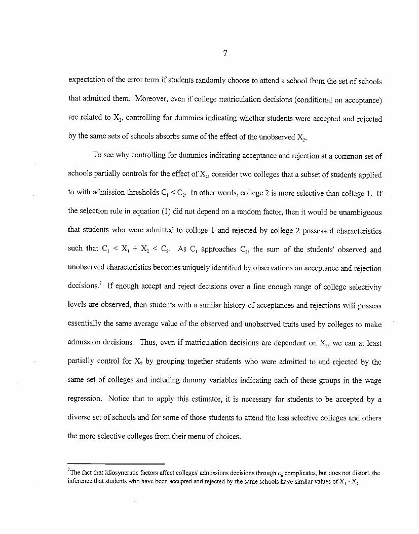
A burgeoning literature has addressed the question, "Does the 'quality' of the college that

students attend influence their subsequent earnings?" Obtaining accurate estimates of thepayoff to

attending a higher quality undergraduate institution is of obvious importance to the parents of

prospective students who foot the tuition bills, and to the students themselves. In addition, because

college selectivity is typically measured by the average characteristics (e.g., average SAT score) of

classmates, the literature is closely coimected to theoretical and empirical studies of peer group

effects on individual behavior. And with higher education making up 40 percent of total

educational expenditures in the United States (see U.S. Department of Education, 1997; Table 33),

understanding the impact of selective colleges on students' labor market outcomes is central for

understanding the role of human capital.2

Past studies have found that students who attended colleges with higher average SAT

scores or higher tuition tend to have higher earnings when they are observed in the labor market.

Attending a college with a 100 point higher average SAT is associated with 3to 7 percent higher

earnings later in life (see, e.g., Kane, 1998). An obvious concern with this conclusion, however,

is that students who attend more elite colleges may have greater earnings capacity regardless of

where they attend school. Indeed, the very attributes that lead admissions committees to select

certain applicants for admission may also be rewarded in the labor market. Most past studies

have used Ordinary Least Squares (OLS) regression analysis to attempt to control for differences in

student attributes that are correlated with earnings and college quality. But college admissions

'The modern literature began with papers by Hunt (1963), Solnion (1973), Wales (1973), Solmon and Wachtel (1975),and Wise (1975), and has undergone a recent renaissance, with papers by Brewer and Ehrenberg (1996), Behrman et al.(1996), Daniel (1997), Kane (1998), and others. See Brewer and Ehrenberg (1996; Table 1) for an excellent summaryof the literature.

2This figure ignores any earnings students forego while attending school, which would increase the relative cost ofhigher education.

decisions are based in part on student characteristics that are unobserved by researchers and

therefore not held constant in the estimated wage equations; if these unobserved characteristics are

positively correlated with wages, then OLS estimates will overstate the payoff to attending a

selective school. Only three previous papers that we are aware of have attempted to adjust for

selection on unobserved variables in estimating the payoff to attending an elite college. Brewer and

Ehrenberg (1996) use a parametric utility maximizing framework to model students' choice of

schools, under the assumption that all students can attend any school they desire. Behrman,

Rosenzweig and Taubman (1996) utilize data on female twins to difference out common

unobserved effects. And Berhman, et al. (1996) use family variables to instrument for college

choice. Our paper complements these previous approaches.

This paper employs two new approaches to adjust for nonrandom selection of students on

the part of elite colleges. In one approach, we only compare college quality and earnings among

students who were accepted and rejected by a comparable set of colleges, and are comparable in

terms of observable variables. In the second approach, we hold constant theaverage SAT score of

the schools to which each student applied, as well as the average SAT score of the school the

student attended, the student's SAT score, and other variables. The second approach is nested in the

first estimator. Conditions under which these estimators provide unbiased estimates of the payoff

to college quality are discussed in the next section. In short, if admission to a college is based on a

set of variables that are observed by the admissions committee and later by the econometrician

(e.g., student SAT), and another set of variables that is observed by the admissions committee (e.g.,

an assessment of student motivation) but not by the econometrician, and if both sets of variables

influence earnings, then looking within matched sets of students who were accepted and rejected by

3

the same groups of colleges can help overcome selection bias.

Bamow, Goldberger and Cain (1981) point out that, "Unbiasedness is attainable when the

variables that determined the assignment rule are known, quantified, and included in the

[regression] equation." Our first estimator extends the concept of "selection on the observables" to

"selection on the observables and unobservables," since information on the unobservables can be

inferred from the outcomes of independent admission decisions by the schools the student applied

to. The general idea of using information reflected in the outcome of independent screens to

control for selection bias may have applications to other estimation problems, such as estimating

wage differentials associated with working in different industries or sizes of firms (where hiring

decisions during the job search process provide screens) and racial differences in mortgage defaults

(where denials or acceptances of applications for loans provide screens).3

We provide selection-corrected estimates of the payoff to school quality using the

College and Beyond dataset, which was recently collected by the Andrew W. Mellon Foundation

and analyzed extensively in Bowen and Bok (1992), and the National Longitudinal Survey of the

High School Class of 1972 (NLS-72). We examine the effect on earnings of several school

quality indicators, including selectivity (as measured by .the school's average SAT score) and net

tuition. Our primary finding is that the financial return to attending a higher quality college falls

considerably once we adjust for selection on the part of the college. Nonetheless, we still find a

substantial payoff to attending schools with higher net tuition. Finally, we examine the impact of

attending a more selective college on students' grades, graduation rates, and post-college

3Braun and Szatrowjcsj (1984) use a related idea to evaluate law school grades across institutions by comparing theperformance of students who were accepted at a common set of law schools but attended different schools.

4

educational attainment.

1. Simulation of Admissions, College Attendance and Earnings

For most students, college attendance involves three sequential choices. First, a student

decides which set of colleges to apply to for admission. Second, colleges independently decide

whether to admit the student to their schools. Third, the student and her parents decide which

college the student will attend from the subset of colleges that admitted her.

We begin by assuming that colleges determine admissions decisions by weighing various

attributes of the student. Indeed, a recent survey by the National Association for College

Admission Counseling indicates that admissions officers consider many factors when selecting

students, including not only students' high school grades and test scores, but also factors such as

their essays, counselor and teacher recommendations, community service, and extracurricular

activities (NACAC Bulletin, November, 1998). Next, we assume that each college uses a threshold

to make admissions decisions. An applicant who possesses characteristics that place him or her

above the college's threshold is accepted; if not, he or she is rejected. Additionally, luckmay enter

into the admission decision.

To proceed analytically, we partition the characteristics that the admissions committee

observes into two sets of variables: a set that is subsequently observable by researchers, denoted X1,

and a set that is unobservable by researchers, denoted X2. The observable set of characteristics

could include factors such as the student's SAT score and high school grade point average (GPA),

whereas the unobservable set could include factors such as assessments of the student's motivation,

ambition and maturity as reflected in her essay, college interview and letters of recommendation.

5

Without loss of generality, assume that X and X2 are scalar variables. We assume a linear

admission rule, in which X1 and X2 have been scaled accordingly. In particular, we assume college

j uses the following rule to admit or reject applicant i:

(1) if Z =X1 + X2 + e.> C then admit to collegej

otherwise reject applicant at college j

where Z is the latent quality of the student as judged by the admission committee, represents the

idiosyncratic, views of college js admission committee, and C is the cutoff quality level the college

uses for admission.4 The term e1 represents luck arid idiosyncratic factors that affect admission

decisions but are unrelated to earnings. We assume ; is independent across colleges. By

definition, more selective colleges have higher values of C.

Now suppose the "structural earnings function" relating income to the students' attributes is:

(2) in W1 = + I3ISAT. + f32X11 + f33X2 +

where SAT. is the average SAT score of matriculants at the college student i attended, X1 and X2

are the two sets of characteristics used by the admission committee to determine admission, and c,

is an idiosyncratic error term that is uncorrelated with the other variables on the right hand side of

(2). Since individual SAT scores are a common X variable, SATJ. can be thought of as the mean

of X1 taken over students who attend college j'. The parameter 13, which may or may not equal

zero, represents the monetary payoff to attending a more selective college.

In practice, researchers have been forced to estimate a wage equation that omits X2:

(3) in = + 'ISATJ + j3'2X1 + u.

4We ignore the possibility of wait listing the student.

6

Even if students randomly select the college they attend from the set of colleges that admitted them,

estimation of (3) will yield biased and inconsistent parameter estimates of 13 and f2. Most

importantly for our purposes, if students choose their school randomly from their set of options, the

payoff to attending a selective school will be biased upward because students with higher values of

the omitted variable, X2, are more likely to be admitted to, and therefore attend, highly selective

schools. Since the labor market rewards X2, and school-average SAT and X2 are positively

correlated, the coefficient on school-average SAT will be biased upward. The coefficient on X1 can

be positively or negatively biased, depending on the relationship between X1 and X,. Also notice

that the greater the correlation between X1 and X2, the lesser the bias in I3I.5

Formally, the coefficient on school-average SAT score is biased upward in this situation

because E(ln W1 SAT.,XI) = 13 + 3ISATJ. + 132X1 + E(u1 X1 + X2 + e1. > The expected

value of the error term (u1) is higher for students who were admitted to, and therefore more likely to

attend, more selective schools.6

If, conditional on gaining admission, students choose to attend schools for reasons that are

independent of X2 and , then students who were accepted and rejected by the same set of schools

would have the same expected value of u. Consequently, our proposed solution to the school

selection problem is to include an unrestricted set of dummy variables indicating groups of students

who received the same admissions decisions (i.e., the same combination of acceptances and

rejections) from the same set of colleges. Including these dummy variables absorbs the conditional

5This should be intuitively clear from considering a situation in which X and X2 are perfectly correlated. In this case,the school average SAT is unaffected by the omitted X2, although the coefficient on X confounds the effect of X andx2.

6A classic reference on selection bias is Heckman (1979).

7

expectation of the error term if students randomly choose to attend a school from the set of schools

that admitted them. Moreover, even if college matriculation decisions (conditional on acceptance)

are related to X2, controlling for dummies indicating whether students were accepted and rejected

by the same sets of schools absorbs some of the effect of the unobserved X2.

To see why controlling for dummies indicating acceptance and rejection at a common set of

schools partially controls for the effect of X2, consider two colleges that a subset of students applied

to with admission thresholds C1 <C2. In other words, college 2 is more selective than college 1. If

the selection rule in equation (1) did not depend on a random factor, then it would be unambiguous

that students who were admitted to college 1 and rejected by college 2 possessed characteristics

such that C1 < X1 + X2 < C2. As C1 approaches C2, the sum of the students' observed and

unobserved characteristics becomes uniquely identified by observations on acceptance and rejection

decisions.7 If enough accept and reject decisions over a fine enough range of college selectivity

levels are observed, then students with a similar history of acceptances and rejections will possess

essentially the same average value of the observed and unobserved traits used by colleges to make

admission decisions. Thus, even if matriculation decisions are dependent on X2, we can at least

partially control for X2 by grouping together students who were admitted to and rejected by the

same set of colleges and including dummy variables indicating each of these groups in the wage

regression. Notice that to apply this estimator, it is necessary for students to be accepted by a

diverse set of schools and for some of those students to attend the less selective colleges and others

the more selective colleges from their menu of choices.

7The fact that idiosyncratic factors affect colleges' admissions decisions throughe13 complicates, but does not distort, theinference that students who have been accepted and rejected by the same schools have similar values of X1 +X2.

8

The following simulations illustrate these points, and suggest that information on a

relatively small number of college application outcomes is sufficient to reduce or eliminate the bias

caused by unobserved variables that influence college admission decisions. For a sample of 4,000

observations, we simulated data as follows. We assume X1, X2 and e1 are standard normal,

independently distributed variables. Every student applies to the same four colleges, and each

college has a different value of C. The values of C are set so that the most selective college admits

approximately the top 12 percent of applicants, the second most selective college admits the top 50

percent, the third most selective college admits the top 70 percent, and the least selective college

admits all applicants. A randomly selected quarter of students choose to attend the best school they

were admitted to, and the remaining students randomly select which college to attend from among

the ones that admitted them.8 We calculate each college's average SAT score by averaging over X1

for the students who attend the college. This acceptance and matriculation process naturally leads

more selective colleges to have higher average SAT scores. We assume the structural wage

equation specified in (2), and set 13 = 0 and 13 = 132 133= 0.5 and draw , from a standard normal

distribution.

Panel A of Table 1 reports average regression statistics from 100 simulations of this model.

As one would expect from the initial assumptions, a regression of mW on SAT, X1 and X2 yields a

coefficient of virtually 0 on school-average SAT (see column 1). If we omit X2 from the model,

however, the coefficient on school-average SAT averages .58 in the simulations, and the coefficient

8Random selection of colleges on the part of students is obviously an unreasonable assumption, but as mentioned, forour selection correction to work all that is required is that the choice of college is independent of the error term in wage

equation (2) and of X2.

9

on X, falls to .42 (see column 2). In column 3 we implement our selection correction method.

That is, we create 16 dummy variables indicating possible combinations of acceptances and

rejections at the 4 schools, and include 15 of these dummies as explanatory variables.'0 Including

these dummy variables drives the coefficient on the school-average SAT score toward 0. Note also

that the coefficient on X1 falls to .26 when the admitlreject dummies are included. This occurs

because X1 + X2 is only controlled imperfectly by the accept/reject dummies, so X1 still has some

independent explanatory power." Consequently, it is inappropriate to interpret the coefficient on X1

as a structural parameter in the selection-corrected model, even though the estimate of 13, is

unbiased.

If the admission rule used by colleges depended only on X,, and if X, were included in the

wage equation, we would have a case of 'selection on the observables" (see Barnow, Cain and

Goldberger, 1981). In this case, however, we have "selection on the observables and

unobservables' since X2 and ej are also inputs into admissions decisions. Nonetheless, as we have

shown, we can control for the bias due to selective admissions by controlling for the groups of

schools at which students were accepted and rejected.

The selection correction works well in this simulation because, conditional on being

9The coefficient on X1 falls because X1 and SAT are positively correlated. Since SAT is positively correlated with X,and X is uncorrelated with X2, the coefficient on SAT is biased up, which in turn causes the coefficient on X to bebiased down. If X1 and X2 are positively correlated, however, the effect of X, could be biased upward.

'°In practice, fewer than 15 dummies were often used because some of the cells were empty. That is, in spite of therandom factor in admissions, there were no simulated students who were rejected by some combination of schoolsand accepted by others.

we control for X1 and the latent variable Z = + e/4 instead of the college application dummies, then the

expected coefficient on X1 still exceeds zero because the coefficient on Z is less than .5due to idiosyncratic errorsin evaluating the candidates. The acceptlreject dummies are also imperfect measures of X1+X2, which is why X1 has

a coefficient that exceeds zero in column 3.

10

accepted, the average SAT score of the school students attend is uncorrelated with the students'

personal characteristics. Indeed, column 4 shows that including three dummy variables indicating

whether a student was admitted to each college has the same effect on the school SAT variable as

controlling for the 16 possible configurations of rejections and acceptances among the 4 schools.

In reality, all students do not apply to the same set of colleges, and it is probably

unreasonable to model students as randomly selecting the school they attend. A complete model of

the two-sided selection that takes place between students and colleges is beyond the scope of the

current paper, but it should be stressed that our selection correction still provides an unbiased

estimate of i3 if students' school enrollment decisions are a function of X1 or any variable outside

the model. The critical assumption is that students' enrollment decisions are uncorrelated with the

error term of equation (2) and X2. If the decision rule students use to choose the college they attend

from their set of options is related to their value of X2, then the bias in the within-matched applicant

model depends on the coefficient from a hypothetical regression of the average SAT score of the

school the student attends on X2, conditional on X1 and the accept/reject dummies. It is possible

that selection bias could be exacerbated by controlling for matched applicant effects. Griliches

(1979) makes this point in reference to twins models of earnings and education. In the current

context, however, if students apply to a fine enough range of colleges, the accept/reject dummies

would control for X2, and the within-matched applicant estimates would be unbiased even if college

choice on the part of students depended on X2. In the following simulation, we assume both

application and matriculation decisions are related to X2 Under these conditions, compared to

estimating equation (3), the proposed selection correction still yields a less biased estimate of

We alter the previous simulation in two respects. First, we assume that the bottom 40

11

percent of students (in terms of X, + X2) only apply to the two least selective schools; the other

students apply to all four schools. Second, we assume that more qualified students are more likely

to attend the most selective school from the set of schools that admitted them. To accomplish this,

we again assume that 25 percent of the students choose to attend the best college that admitted

them, but for this simulation, we randomly select this 25 percent from the top half of the applicant

pooi (i.e., those students with X,+X2> 0). All of the other students (which includes the bottom 40

percent of students who applied to two schools and the next 10 percent who applied to four)

randomly choose which school to attend from the set that admitted them. Panel B provides results

from simulating such a model 100 times. Although school-average SAT has a positive effect on

earnings in all the models that omit X2, it is less than half as large when we include 17 dummies

indicating the configurations of acceptances and rejections for the students who applied to the same

set of schools.'2 Also notice that in this simulation, the effect of school-average SAT is smaller in

the model that controls for the 17 accept/reject configurations than in the model that includes 3

dummies indicating acceptance at each college.

Another factor that would be expected to influence student matriculation decisions is

financial aid. By definition, merit aid is related to the school's assessment of the student's potential.

Past studies have found that students are more likely to matriculate to schools that provide them

with more generous financial aid packages (see, e.g., van der Klaauw, 1997). If more selective

colleges provide more merit aid, the estimated effect of attending an elite college will be biased

upward because relatively more students with higher values of X2 will matriculate at elite colleges,

'2There are 2 more dummy variables in this simulation than in the previous simulation because there are two morecombinations of acceptances and rejections representing the students that apply to only two schools.

12

even conditional on the outcomes of the applications to other colleges. The relationship between

aid and school selectivity is likely to be quite complicated, however. Breneman (1994; Chapter 3),

for example, finds that the middle ranked liberal arts colleges provide more financial aid than the

highest ranked and lowest ranked liberal arts colleges. If students with higher values of X2 are

more likely to attend less selective colleges because of financial aid, the selectivity bias could be

negative instead of positive.

Also notice that if students choose the college they attend based on 8, the error in the

structural wage equation, then the selection-bias adjustment could lead to more or less biased

estimates. The bias would depend on the coefficient on SAT from a hypothetical regression of s on

SAT, X1, and the accept/reject dummies.

Finally, an alternative though related approach to modelling unobserved student selection is

to assume that students are knowledgeable about their academic potential, and reveal their potential

ability by the choice of schools they apply to. Indeed, students may have a better sense of their

potential ability than college admissions committees. To cite one prominent example, note that

Steven Spielberg was rejected by both USC and UCLA film schools (Grover, 1998). It is plausible

that students with greater observed and unobserved ability are more likely to apply to more

selective colleges. In this situation, the error term in equation (3) could be modelled as a function

of the average SAT score (denoted AVG) of the schools to which the student applied: u = +

'r1AVG + v1. If v is uncorrelated with the SAT score of the school the student attended, we can

solve the selection problem by including AVG in the wage equation. When we implement this

approach, we also include dummy variables indicating the number of schools the students applied

to. We call this approach the "self-revelation" model because individuals reveal their unobserved

13

quality by their college application behavior. Notice also that the average SAT score of the schools

the student applied to, and the number of applications they submitted, would be absorbed by

including unrestricted dummies indicating students who were accepted and rejected by the same

sets of schools; therefore, the self-revelation model is a special case of our first selection correction

model.

2. Data and Comparison to Previous Literature

The College and Beyond (C&B) Survey is described in detail in Bowen and Bok (1998,

Appendix A). In short, the starting point for the C&B database was the institutional records of

students who enrolled in (but did not necessarily graduate from) one of 34 colleges in 1951, 1976

and 1989. These institutional records were linked to a survey administered by Mathematica Policy

Research, Inc. for the Andrew W. Mellon Foundation in 1995-97 and to files provided by the

College Entrance Examination Board (CEEB) and the Higher Education Research Institute (HERI)

at the University of California, Los Angeles. We focus here on the 1976 entering cohort. While

survey data are available for 23,572 students from this cohort, we exclude students from four

historically black colleges and universities, and for most of our analysis we restrict the sample to

those who were working full time. The 30 colleges and universities in our sample, as well as their

average SAT scores and tuition, are listed in Appendix Table A. Our final sample consists of

14,239 full-time, full-year workers.

The C&B institutional file consists of information drawn from students' applications and

transcripts, including variables such as students' GPA, major and SAT scores. These data were

collected for all matriculants at the C&B private schools; for the four public universities, however,

14

data were collected for a subsample of students, consisting of all known minority students, all

varsity letter-winners, all students with combined SAT scores of 1,350 and above, and a random

sample of all other students. We developed weights so that the sample is nationally representative

of public and private universities and liberal arts colleges.13

The C&B institutional data were linked to files provided by HERI and CEEB. The CEEB

file contains information from the Student Descriptive Questionnaire (SDQ), which students fill out

when they take the SAT exam. We use students' responses to the SDQ to determine their high

school class rank and parental income. The file that HERI provided is based on data from a

questionnaire administered to college freshman by the Cooperative Institutional Research Program

(CIRP). We use this file to supplement C&B data on parental occupation and education.

Finally, the C&B survey data consist of the responses to a questionnaire that most

respondents completed by mail in 1996, although those who did not respond to two different

mailings were surveyed over the phone. The survey response rate was approximately 80 percent.

The survey data include information on 1995 annual earnings, occupation, demographics,

education, civic activities, and satisfaction.'4 Importantly for our purposes, early in the

questionnaire respondents were asked, "In rough order of preference, please list the other schools

13We use Carnegie Classifications to define these categories. The public and private universities include allDoctorate-Granting Institutions (Research I and II and Doctorate I and II), and the liberal arts colleges include theLiberal Arts Colleges I.

'4The C&B survey asked respondents to report their 1995 pre-tax annual earnings in one of the following ten intervals:less than $1,000; $1 ,000-$9,999; $1 0,000-s19,999; $20,000-$29,999; $30,000-$49,999; 550,000-74,999; 575,000-100,000; 5100,000-5149,999; $l50,000-$199,999, and more than $200,000. We converted the lowest nine earningscategories to a cardinal scale by assigning values equal to the midpoint of each range, and then calculated the naturallog of earnings. For workers in the topcoded category, we used the 1990 Census (after adjusting the Census data to1995 dollars) to calculate mean log earnings for college graduates age 36-38 who earned more than $200,000 per year.

15

you seriously considered."15 Respondents were then asked whether they applied to, and were

accepted by, each of the schools they listed.'6 By linking the school identifiers to a file provided by

HERI, we determined the average SAT score of each school that each student applied to. This

information enabled us to form groups of students who applied to a similar set of schools and

received the same admissions decisions (i.e., the same combination of acceptances and rejections).

Because there were so many colleges to which students applied, we considered schools equivalent

if their average SAT score fell into the same 25 point interval. For example, iftwo schools had an

average SAT score between 1200 and 1225, we assumed they used the same admissions cutoff.

Then we formed groups of students who applied to, and were accepted and rejected by,

"equivalent" schools.'7

Table 2 illustrates how we would construct 5 groups of matched applicants for 15

hypothetical students. Students A and B applied to the exact same three schools and were accepted

and rejected by the same schools, so they were paired together. The four schools to which students

C, D, and E applied were sufficiently close in terms of average SAT scores that they were

considered to use the same admission standards; because these students received the same

5Students who responded to the C&B pilot survey were not asked this question, and therefore are excluded from ouranalysis.

16Students could have responded that they couldn't recall applying or being accepted, as well as yes or no. They wereasked to list three colleges other than the one they attended that they seriously considered. In addition, prior to thequestion on schools the student seriously considered, respondents were asked "which school did you most want toattend, that is, what was your first choice school?" If that school was different from the school the student attended,there was a follow-up question that asked whether the student applied to their first-choice school, and whether theywere accepted there. Consequently, infonnation was collected on a maximum of 4 colleges to which the student couldhave applied, in addition to the college the student attended.

'7Students who applied to only one school were not included in these matches.

16

admissions decisions from comparable schools, they were categorized as matched applicants.

Students were not matched if they applied to only one school (students F and G), or if no other

student applied to a set of schools with similar SAT scores (student 0). Five dummy variables

would be created indicating each of the matched sets.

Table 3 provides weighted means and standard deviations for men and women in the

sample who were employed full time in 1995. Everyone in the sample attended a C&B school as a

freshman but did not necessarily graduate from the school (or from any school). Nearly 70 percent

of students in the unweighted data listed at least one other school they applied to in addition to the

school they attended, whereas just over half of the students in the weighted sample reported

applying to at least one additional school. This difference stems from the fact that students from

public universities receive much more weight in the weighted sample than unweighted sample, and

students who attended public universities were less likely to report applying to another school that

they seriously considered attending. Among students who were accepted by more than one school,

59 percent chose to attend the most selective school to which they were admitted. We were able to

match 44 percent of the students with at least one other student in the sample on the basis of the

schools that they were accepted and rejected by. Summary statistics are also reported for the

subsample of matched applicants. It is clear that the C&B sample is very selective. The mean

annual earnings in 1995 for full-time, full-year workers is $89,026 for the male sample and $76,859

for the pooled sample of men and women, both of which are high even for college graduates. The

studentsT average SAT score (Math plus Verbal) exceeds 1,100. Nearly 40 percent of the sample

was ranked in the top 10 percent of their high school class.

Because the schools included in the C&B sample are highly selective, with average SAT

17

scores ranging from 1,020 to 1,360, we first compared the payoff to attending a more selective

school in the C&B sample to corresponding estimates from representative national samples of

college graduates. In Table 4 we replicate as closely as possible the wage regressions reported by

Kane (1998) and Daniel, Black and Smith (1997). Kane analyzes a pooled sample of men and

women from the High School and Beyond (HSB) Survey, whereas Daniel, et al. use a sample of

men from the National Longitudinal Survey of Youth (NLSY). In both studies, college selectivity

is measured by the average SAT of students who attend each college, as reported by the

institution.18 These estimates indicate that attending a school with a 100 point higher average SAT

score is associated with 5 to 8 percent higher earnings later in life, but the estimates based on the

C&B survey are slightly higher than the corresponding estimates from the NLSY and especially the

HSB. Brewer, Eide and Ehrenberg (1999) provide evidence that the payoff to attending an elite

college increased between 1986 and 1992, which could account for the larger C&B estimates. In

the next section, we examine whether these estimates are confounded by unobserved student

attributes.

3. The Effect of College Selectivity on Earnings

Tables 5a and Sb present our main set of log-earnings regressions. We limit the sample to

full-time, full-year workers, and estimate separate Weighted Least Squares (WLS) regressions for a

t8For the C&B survey, we based school-average SAT scores on a data file provided by HERI. HERI collects SATscore data from college guidebooks; the scores in the guidebooks are generally based on the schools' responses tosurveys. The correlation between the HERI SAT scores and the school averages calculated from the students in theC&B database for 30 schools is .94. The mean, however, is 25 points higher in the HERI data. We use the HERI datato be comparable with the previous literature (e.g., Kane, 1998), and because we do not have data on average SATscores for schools outside the C&B universe.

18

pooled sample of men and women (Table 5a), and for the subset of men (Table 5b).'9 The reported

standard errors are robust to correlation in the errors among students who attended the same

college. With the exception of a dummy variable indicating whether the student participated on a

varsity athletic team, the explanatory variables are all determined prior to the time the student

entered college. Most of the covariates are fairly standard, although an explanation of the

"predicted log parental income" variable is necessary. Parental income was missing for many

individuals in the sample. Consequently, we predicted income by first regressing log parental

income on mother's and father's education and occupation for the subset of students with available

family income data (see Appendix Table 2), and then multiplying the coefficients from this

regression by the values of the explanatory variables for every student in the sample.

The basic model, reported in the first column of Tables 5a and Sb, is comparable to the

models estimated in much of the previous literature in that no attempt is made to adjust for selective

admissions. In Table 5a, the basic model indicates that students who attended a school with a 100

point higher average SAT score earned about 6 percent higher earnings in 1995, holding constant

their own SAT score, race, gender, parental income, athletic status, and high school rank. For the

sample of men in Table 5b, the basic model shows that the effect of a 100 point higher school-

average SAT score on earnings is similar, about 7 percent.

Column 2 presents the "matched applicant" model, which adjusts for selection by including

dummy variables that indicate students who were accepted and rejected by the same sets of schools.

As mentioned earlier, to form these groups we treat schools with average SAT scores in the same

25 point range as identical. We were able to match 6,335 students with at least one other student

19The sample of women was too small to draw precise estimates from, but the results were qualitatively similar.

19

who applied to, and was accepted and rejected by, an equivalent set of institutions. Including

dummies for the sets of matched students renders the effect of school-average SAT

indistinguishable from zero in column 2 for both of the samples. The standard error doubles when

we look within matched sets of students, but for the pooled sample, we can reject an effect of

around 3 percent higher earnings for a 100 point increase in the school-average SAT score; that is,

we can reject an effect size that is smaller than that found in most of the previous literature. The

weaker effect of school SAT in the matched applicant models is not just a result of idiosyncracies

of the restrictive matched applicant samples; if we estimate the basic model in column 1 for the

matched applicant subsample, the results are qualitatively similar to those from the full sample.

Figure 1 illustrates the college application and attendance patterns of the most common sets

of matched applicants (i.e., those sets that include at least 15 students). The length of the bars

indicates the range of schools to which each set of matched students applied, and the shaded area of

each bar represents the range of schools that each set of students actually attended. As shown by

the figure, most students reported applying to a relatively narrow range of schools insofar as SAT

scores are concerned,2° and the range of schools that students attended is even narrower, The

average range of school-average SAT scores of students who were accepted by at least two schools

was 139 points.2' Furthermore, dummies indicating the groups of matched students account for 85

percent of the variability of in the average SAT scores of the schools the students actually attended.

201t is possible that the range of schools is particularly circumscribed because the C&B survey asked respondents toreport the schools they "seriously considered."

21This figure refers to the average range of school-SAT scores for the schools that accepted the students. The averagerange of school-average SAT scores for the schools that students applied to (regardless of whether they were accepted)was 158 for students who applied to more than one school.

20

Thus, it is possible that the restricted variability used to identify the effect of school selectivity

within matched groups of students does not influence earnings, whereas an experiment that moved

students from a school with a 1,000 average SAT score to one with a 1,300 average would have a

substantial effect on students! earnings. Although the latter experiment is relevant for larger

considerations of education policy (such as affirmative action), specific instances of students who

considered attending such a wide range of schools are rare. For parents and students, however, the

relevant comparison is among the set of schools that admitted the student.

Our second model that adjusts for selection, the "self-revelation" model, is shown in column

3 of Tables 5a and 5b. This model includes the average SAT score of the schools to which students

applied, and dummy variables indicating the number of schools to which students applied. The

effect of school-average SAT score is qualitatively similar in the self-revelation and matched

applicant models. In the self-revelation model for both of the samples, the effect of school-average

SAT in colunm 3 is close to zero, and more precisely estimated than in the matched applicant

model. Results of the self-revelation models are similar to those of the matched applicant models

because students who apply to schools with the same mean SAT tend to apply to a fairly narrow

range of schools around that mean. The average SAT score of the schools students applied to

accounts for 62 percent of the variability in the SAT score of the schools students attended.

Table 6 presents parameter estimates from models that are similar to the self-revelation

model, but use alternative selection controls in place of the average SAT score of the schools to

which the student applied. For example, the third row reports estimates from a model that controls

for the average SAT score of the schools at which the student was accepted. The results of this

model are similar to those in the self-revelation model in row 2, in that the effect on earnings of the

21

average SAT score of the school that the student attended is indistinguishable from zero. We also

obtain similar results when we control for the highest school-average SAT score among the

colleges that accepted the student (row 4) or the highest school-average SAT score among the

colleges to which the student applied (row 5). Moreover, we consistently find that the average SAT

score of the schools the student applied to, but either was rejected by or chose not to attend, has a

large effect on earnings. For example, results from the model in row 7 show that a 100 point

increase in the highest school-average SAT score among the colleges at which the student was

rejected is associated with an 8 percent increase in earnings. These results raise doubt about a

causal interpretation of the effect of attending a school with a higher average SAT score in

regressions that do not control for selection.

A. Results for National Longitudinal Survey of the High School Class of 1972

To explore the robustness of our results in a nationally representative data set, we analyzed

data from the National Longitudinal Study of the High School Class of 1972 (NLS-72). We restrict

the NLS-72 sample to those students who started at a four-year college or university in October of

1972, and we use 1985 annual earnings data from the fifth follow-up survey. In 1985 the NLS-72

respondents were about six years younger than the C&B respondents were in 1995 (typically 31

versus 37). In the first follow-up survey, the NLS-72 asked students questions about other schools

to which they may have applied in a fashion similar to the C&B survey.22 The NLS-72 also

22Specifically, respondents were asked, 'When you first applied, what was the name and address of the FIRST school orcollege of your choice? Were you accepted for admission at that school?" These questions were repeated for therespondents' second and third choice schools. We matched the responses to these questions to the HERI file todetermine the average SAT score in 1973 of the schools that students applied to.

22

contains detailed information about student& academic and family backgrounds, allowing us to

construct most of the same variables used in Table 5•23 The NLS-72 survey did not, however,

collect information on respondents' full-year work status in 1985. We include in the sample all

NLS-72 respondents (regardless of how much they worked) whose annual earnings exceeded

$5,000.

The means and standard deviations for the NLS-72 sample, as well as regression estimates,

are reported in Table 7. Because the NLS-72 sample is relatively small (2,127 workers), we could

not estimate the matched applicant model; however, we were able to estimate the basic regression

model and self-revelation model for a pooled sample of men and women. The basic model without

application controls, in column 2, indicates that a 100 point increase in the school-average SAT

score is associated with approximately 5.1 percent higher annual earnings. However, the self-

revelation model reported in column 3 suggests that the effect of school-average SAT score is close

to zero, although the standard error of .023 makes it difficult to draw a precise inference. The

school SAT score estimates based on the comparable C&B sample are strikingly similar: the

coefficient (standard error) on school-average SAT score was .055 (.019) in the basic model and

-.022 (.017) in the self-revelation model using the C&B sample and imposing similar sample

restrictions (in 1995 dollars). These results suggest that our findings in Tables 5a and 5b are not

unique to the schools covered by the C&B survey.

23We have parental income data for most of the NLS-72 sample, allowing us to control for actual, rather than predicted,parental income. We do not include a dummy variable for athletes because NLS-72 does not identify varsity letterwinners.

23

B. Interactions Between School-Average SAT and Student Characteristics

Table 8 reports another set of estimates of the three models using the C&B data set (basic,

matched applicant, and self-revelation model) augmented to include an interaction between school-

average SAT and predicted log parental income. For the pooled sample of men and women, in all

the models we estimated the coefficient on the interaction between parental income and school-

average SAT is negative, indicating a higher payoff to attending a more selective college for

children from lower income households. The interaction term is statistically significant and

generally has a sizable magnitude. For example, based on the self-revelation model in column 3 of

Table 8, the gain from attending a college with a 200 point higher average SAT score for a family

whose predicted log income is two standard deviations below the mean is 7 percent, versus

virtually nil for a family with mean income.

In results not reported here, we also experimented with adding a variable to each model in

Table 5a that interacted the students' own SAT score and the average SAT score of the school they

attended. These estimates uniformly yielded significant negative effects on the own SAT-school

SAT interaction term. Moreover, if we further allow for an asymmetric effect of the own SAT-

school SAT interaction for students whose SAT scores exceeded the school average (i.e., by also

including the product of a dummy variable indicating students whose SAT score exceeded their

school average and the interaction between school and own SAT), we continue to fmd negative

effects of the interactions between own SAT and school SAT. Thus, there is no evidence in these

data that students who score relatively low on the SAT exam do worse in the labor market by

attending schools with a relatively high average SAT.

24

C. The Effect of Other College Characteristics on Earnings

Although the average SAT score of the school a student attends does not have a robust

effect on earnings once selection on unobservables is taken into account, we do find that the school

a student attends is systematically related to his or her subsequent earnings. In particular, if we

include 30 unrestricted dummy variables indicating school of attendance instead of the average

SAT score in each of the models in Tables 5a and 5b, we reject the null hypothesis that schools are

unrelated to earnings at the .01 level. Thus, something about schools appears to influence earnings.

A possible reason for the insignificance of school-average SAT in the selection-adjusted models is

that the average SAT score is a crude measure of the quality of one's peer group. Since, to some

extent, all schools enroll a heterogeneous group of students, it might be possible for students to seek

out the type of peer group they desire if they had attended any of the schools that admitted them.

An able student who attends a lower tier school can find able students to study with, and, alas, a

weak student who attends an elite school can find many other weak students to not study with. Our

within-group models may place too much emphasis on an imperfect measure of school selectivity.

Therefore, we next examine the effect of other college characteristics on students' subsequent

earnings. First, we explore the effect on earnings of the dispersion in SAT scores within a school.

Then we examine the return to the schools' average tuition costs (net of financial aid) and to their

expenditures per student.

For each school in the C&B data set, we calculated the standard deviation of SAT scores

among freshmen in 1976. The standard deviation of within-school SAT scores ranged from 118 to

170 across schools, and the average standard deviation was 150 points. Across these colleges, the

correlation between the average SAT score and standard deviation of scores is -.39, which is

25

consistent with less selective schools imposing a lower admissions threshold and attracting a more

diverse student body in terms of achievement levels. We estimated a series of regressions in which

we included the school-average SAT score, cross-sectional standard deviation of scores, and

interaction between these two variables, in addition to the other variables in Table 5. The pattern of

results was similar for the three models we estimated. The estimated coefficients and standard

errors from the self-revelation model for the pooled sample of men and women are reported below

(4) In W = .77 SAT + 6.10 SD -.53 SAT*SD + other variables(.44) (3.49) (.30)

where SAT is the school-average SAT (divided by 100), SD is the school standard deviation of

SAT scores (divided by 100) and SAT*SD is the product of these two variables. Interestingly, each

of the variables is on the margin of being individually statistically significant. The mean and

dispersion of SAT scores among students in a college have a complex relationship with student

earnings. A higher school-average SAT score is negatively associated with earnings for a college

with dispersion in SAT scores greater than or equal to the average standard deviation of scores for

this sample of 30 colleges. For the top two-thirds of the schools in our sample in terms of average

SAT scores, greater dispersion in SAT scores is negatively associated with earnings.24

Table 9 presents models in which the logarithm of college tuition costs net of average

student aid is the school quality indicator.25 For the pooled sample of men and women, these

models indicate that students who attend higher tuition schools earn more after entering the labor

24This result is consistent with Hoxby and Terry (1998), although they do not present results controlling forselection on unobserved student characteristics.

25Net tuition for 1970 and 1980 was calculated by subtracting the average aid awarded to undergraduates from thesticker price tuition, as reported in the 11th and 12" editions of American Universities and Colleges. Then the 1976net tuition was interpolated from the 1970 and 1980 net tuition, assuming an exponential rate of growth.

26

market. The magnitude of the coefficient on tuition falls in the models that adjust for school

selection, but remains sizable. For example, the coefficient of .050 in column 5implies an internal

real rate of return of approximately 16 percent for a person who begins work after attending college

for four years, then earns mean 1995 income throughout his career and retires 44 years later.26 The

coefficient in column 3 implies an internal real rate of return of 18 percent. Notice also that the

coefficient on the interaction term for parental income and tuition (shown in columns 2, 4, and 6) is

negative, indicating that there is a higher payoff to attending a more expensive school for children

from low-income families. Although the implied internal rates of return to investing in a more

expensive college in Table 9 are extremely high, one should recognize that the cost of education has

roughly doubled in real terms since the late 1 970s, and the payoff to education increased in general

since the late 1 970s. The implicit internal real rate of return for the estimate in column 5 of Table 9

falls to 9 percent if tuition costs are doubled. Indeed, the supernormal return to investing in high-

tuition education in the 1 970s may explain why it was possible for colleges to raise tuition so much

inthe 1980s and 1990s.

College tuition may have a significant effect on subsequent earnings because schools with

higher tuition may provide their students with more, or higher quality, resources. We next

summarize estimates of the effect of expenditures per student on subsequent earnings. Interestingly,

the correlation between tuition and total expenditures per student in our sample of schools is less

than .30, so differences in tuition probably result from factors in addition to spending per student,

such as the value of the schooPs endowment and public support. One should also recognize

26This rate of return would fall to 14 percent if we assumed that the person spent 1.5 years in graduate school (theaverage time spent in graduate school for the C&B sample) immediately after college.

27

limitations of our measures of expenditures per students: (1) undergraduate and graduate student

expenditures are combined; (2) there are inherent difficulties classifying instructional and non-

instructional spending; and (3) expenditures are lumpy over time.

To directly explore the effect of school spending, we included either the log of total

expenditures per student (undergraduate and graduate), or the log of instructional expenditures per

student, in place of tuition in the earnings equation.27 Both measures of expenditures per pupil had

a statistically significant and large impact on earnings in the basic model for the pooled sample of

men and women. When we estimated the matched applicant model and the self-revelation model,

the effect of expenditures per pupil was smaller, and less precisely estimated. Although the effect

of expenditures per pupil was statistically insignificant, the coefficient was positive in all but one of

the models, and implied substantial internal rates of return to school spending.28 These results

provide mixed evidence on the effect of expenditures per student on students' subsequent income,

perhaps because spending per student is poorly measured.

D. Estimates for Black Students

Because of interest in the effect of affirmative action in admissions by more selective

schools, we have estimated all the preceding models separately for black students using the C&B

data set. Unfortunately, the sample of black students who enrolled in these schools in 1976 is

relatively small -- only 839 full-time workers. Consequently, our results are imprecise.

27We use 1976 expenditure data from the Integrated Postsecondary Education Data System (IPEDS) Survey.

28The coefficient (and standard error) on log instructional expenditures per student if this variable was included insteadof tuition in column 1, 3 and 5 of Table 9 were: .096 (.047); .073 (.082); and .036 (.045). The correspondingcoefficients for log total expenditures per student were: .110 (.066); -.009 (.088); and .041 (.068).

28

Nonetheless, there is no evidence that the relationship between school selectivity and subsequent

earnings is different for black students. For example, when we estimate the model in column 1 of

Table 5a for black students, the coefficient (and standard error) on school-average SAT is .060

(.025). The coefficient falls to .024 (.030) if the self-revelation model in column 3 is estimated.

Similar to all students, black students who attended higher tuition schools had higher earnings when

they joined the labor market, and the magnitudes on the coefficients were comparable to the

estimates for the full sample. In general, these data suggest that black students benefit from

attending more selective colleges just as much as other students, but we cannot draw a strong

inference because of the small number of black students in our sample in 1976.

4. Academic Outcomes

Finally, we examined the relationship between school selectivity and three academic

outcomes: the students' college grade point average (GPA), probability of graduating from the

college they first attended, and probability of obtaining a post-college degree Because of

differences in grading schemes and generosity across schools, we measure grades within colleges,

by the students' GPA percentile rank in their class. For each outcome, we estimated a linear

probability model for each of our three classes of models using the pooled sample of men and

women. Results are reported in Table 10.

In all three classes of models, students who attended a college with a higher average SAT

score tended to have a lower rank in the class, other things equal.29 For example, according to the

29Bowen and Bok (1998) report a similarresult.

29

basic model, students who attended a college with a 100 point higher average SAT score tended to

graduate 5.6 percentile ranks lower in their class. The corresponding deficit was 7.8 percentile

ranks in the matched applicant model and 6.4 percentile ranks in the self-revelation model. The

improvement in class rank for students who choose to attend a less selective college may help

explain why those students do not appear to incur lower earnings; employers (and graduate schools)

may value their higher class rank by enough to offset any other effect of attending a less selective

college on earnings. If we add class rank to the wage regressions in Table 5a, we find that students

who graduate 7 percentile ranks higher in their class earn about 3.2 percent higher earnings, which

may largely offset any advantage of attending an elite college on earnings.

Lastly, Table 10 provides mixed evidence for the effect of school-average SAT on

graduation rates and advanced degrees. The effect of school-average SAT score on graduation rates

is indistinguishable from zero in all three models. On the other hand, school-average SAT score

has a positive and significant effect on the probability of obtaining an advanced degree in both the

basic model and the self-revelation model; however, the effect is statistically insignificant in the

matched applicant model.

5. Conclusion

The colleges that students attend are affected by selection on the part of the schools that

students apply to, and by selection on the part of the students and their families from the menu of

feasible options. A major concern with past estimates of the payoff to attending an elite college is

that more selective schools tend to accept students with higher earnings capacity. This paper

adjusts for selection on the part of schools by comparing earnings and other outcomes among

30

students who applied to, and were accepted and rejected by, a comparable set of institutions.

Although our selection correction has many desirable features, a complete analysis of school

selection also would model students' choice of colleges. Nonetheless, since college admission

decisions are made by professional administrators who have much more information at their

disposal than researchers who later analyze student outcomes, we suspect that our selection

correction addresses a major cause of bias in past wage equations.

After we adjust for students' unobserved characteristics, our fmdings cast doubt on the view

that school selectivity, as measured by the average SAT score of the freshmen who attenda college,

is an important determinant of students' subsequent incomes. Students who attendedmore selective

colleges do not earn more than other students who were accepted and rejected by comparable

schools but attended less selective colleges. Additional evidence of omitted variable bias due to the

college application and admissions process comes from the fact that the average SAT score of

schools that a student applied to but was rejected from has a stronger effect on the student's

subsequent earnings than the average SAT score of the school the student actually attended. These

results are consistent with the conclusion of Hunt's (1963; p. 56) seminal research:

The C student from Princeton earns more than the A student from Podunk not mainlybecause he has the prestige of a Princeton degree, but merely because he is abler. Thegolden touch is possessed not by the Ivy League College, but by its students.

Even after adjusting for selection, however, we do find that the school a student attends

affects his or her subsequent income. The characteristics of schools that influence students'

subsequent income appear to be better captured by average tuition costs than by the school's

average SAT score. Indeed, we find that students who attend colleges with higher average tuition

costs tend to earn higher income years later. The internal real rate of return on college tuition for

31

students who attended college in the late 1 970s was quite high, in the neighborhood of 16 to 18

percent. But college tuition costs have risen considerably since the 1 970s, driving the internal rate

of return to a more normal level.

Finally, we find that the returns to school characteristics such as average SAT score or

tuition are greatest for students from more disadvantaged backgrounds. School admissions and

financial aid policies that have as a goal attracting qualified students from more disadvantaged

family backgrounds may raise national income, as these students appear to benefit most from

attending a more elite college. Eliwood and Kane's (1998) recent finding that college enrollment

hardly increased for children from low-income families in the 1980s is troubling in this regard.

32

References

American Council on Education, American Universities and Colleges, 12thedition (Hawthorn, NewYork: Walter de Gruyter, 1983).

Barron's, 1982, Barron's Profiles of American Colleges (Woodbury, NY: Barron's EducationalSeries, 12th edition).

Bamow, Burt S., Glen G. Cain and Arthur Goldberger, "Selection on Observables," EvaluationStudies Review Annual, 5:43-59, 1981.

Behrman, Jere R., Jill Constantine, Lori Kletzer, Michael McPherson, and Morton 0. Schapiro,"The Impact of College Quality on Wages: Are There Differences Among Demographic Groups?"Working Paper No. DP-38, William College, 1996.

Behrman, Jere R., Mark R. Rosenzweig and Paul Taubman, "College Choice and Wages: EstimatesUsing Data on Female Twins," Review of Economics and Statistics, 78 (4), 1996, pp. 672-85.

Bowen, William G., and Derek Bok, The Shape of the River: Long-Term Consequences ofConsidering Race in College and University Admissions (Princeton, NJ: Princeton UniversityPress, 1998).

Braun, Henry and Ted Szatrowski, "The Scale-Linkage Algorithm: Construction of a UniversalCriterion Scale for Families of Institutions," Journal of Educational Statistics 9, 1984, pp. 311-330.

Breneman, David W. Liberal Arts Colleges: Thriving, Surviving or Endangered (Washington,D.C.: The Brookings Institution, 1994).

Brewer, Dominic and Ronald Ehrenberg, "Does it Pay to Attend an Elite Private College? Evidencefrom the Senior High School Class of 1980" in Research in Labor Economics, vol. 15, pp. 239-71.

Brewer, Dominic, Eric Eide and Ronald Ehrenberg, "Does it Pay to Attend an Elite College? CrossCohort Evidence on the Effects of College Type on Earnings," Journal of Human Resources 34 (1),Winter 1999, pp. 104-23.

Daniel, Kermit, Dan Black, and Jeffrey Smith, "College Quality and the Wages of Young Men,"Research Report No. 9707, Department of Economics, University of Western Ontario, 1997.

Ellwood, David and Thomas Kane, "Who is Getting a College Education: Family Background andthe Growing Gaps in Enrollment," Mimeo., Kennedy School of Government, September 1998.

Fumiss, Todd W., ed. American Universities and Colleges ,11th edition (Washington D.C.:American Council on Education, 1973).

33

Griliches, Zvi, "Sibling Models and Data in Economics: Beginnings of a Survey," Journal ofPolitical Economy, 87 (5), 1979, pp. S37-S64.

Grover, Ronald, "How Steven Spielberg Sustains His Creative Empire," Business Week, July 13,1998, p. 96.

Heckman, James, "Sample Selection Bias as a Specification Error," Econometrica 47 (1), 1979, pp.153-6 1.

Hoxby, Caroline, and Bridget Terry, "Explaining Rising Income and Wage Inequality Among theCollege-Educated," Mimeo., Harvard University, April, 1999.

Hunt, Shane, "Income Determinants for College Graduates and the Return to EducationalInvestment." Unpublished Ph.D. Disseration, Yale University, 1963.

Kane, Thomas, "Racial and Ethnic Preferences in College Admission," in The Black-White TestScore Gap, edited by C. Jencks and M. Phillips, Washington, D.C.: Brookings Institution, 1998.

National Association for College Admission Counseling, "Survey Examines Trends," the NACACBulletin, November, 1998, p. 1.

Solmon, Lewis, "The Definition of College Quality," in Does College Matter: Some Evidence onthe Impacts of Higher Education, edited by Lewis Solmon and Paul Taubman (New York:Academic Press, 1973).

Solmon, Lewis, and Paul Wachtel, "The Effects on Income of Type of College Attended,"Sociology of Education 48, 1975, pp. 75-90.

U.S. Department of Education, National Center for Education Statistics, Digest of EducationStatistics 1997, NCES 98-015, Washington, D.C., 1997.

Van der Klaauw, Wilbert, "A Regression-Discontinuity Evaluation of the Effect of Financial AidOffers on College Enrollment," Mimeo., Department of Economics, NYU, October 1997.

Wales, Terence, "The Effect of College Quality on Earnings: Results from the NBER-ThorndikeData," Journal of Human Resources 8, 1973, pp. 306-17.

Winston, Gordon, and Ivan Yen, "Costs, Prices, Subsidies, and Aid in U.S. Higher Education,"Working Paper DP-32, Williams College, July, 1995.

Wise, David, "Academic Achievement and Job Performance," American Economic Review 65,1975, pp. 350-66.

</ref_section>

U)

Cu

C.)

C

) C

.)

0 C

) U

) .

C.)

w

>

C

) •C

C

) 0

C)

C-

C.

U)

0 0 .

C)

U)

'4-

0 C

) C

) C

u C

) I-

C

) LI

_c

0 —

o C

--

0 LU

cQ)

C . a

4-.

(N

Cu

j.-—

O

(

o —E

Li)

(0

>-

C . o

C.

0D

C.

cCC

)

- —

- CC

-=

- ) C.

o 0C)a

) . •=U

).C

e

(0O

JJ

Li)

1*. - o

U)

0U)

,-<

(I)

U)

C)

C)

Cu

>—

_ (jCI)

U)

C)

Li)•

>

<

-Li)0

•.- C) -

'4..

0

C,

—

C)

CLi

)C

C)

C

Cu

Q

—(0

C

(Si

C- 0

215;

- C

o c W

u,u,

C

LU

C,

U) 0 U) 0 U) 0 U) 0 U) 0 U) 0 U) 0

N 0 N

-

U) N 0 N-

U) N 0 N-

U) N 0 ()

C') N

N

N

N

- — - - 0 0 0 0 - '- - - - '- - '- '- '- '- '- - -

01

p8!d

dy

sioo

qos y jo

aioo

e6ie

Ay

U)

N-

C)

Table IAverage Regression Statistics from Simulating Selection Correction Model 100 Times

Panel A: All Students Apply to Four Schools; Random Matriculation

15 dummies for College Acceptance

and Rejection Configurations1

3 dummies indicating

College Acceptance

R2

Parameter EstimatesModel

(1) (2) (3)Variable

Intercept

School Average SATJ*

X1 (e.g., own SAT)

X2(e.g., unobserved ability)

0.50

(0.02)

0.58

(0.05)

0.42

(0.02)

0.50

(0.02)

0.01

(0.05)

0.50

(0.02)

0.50

(0.02)

0.59

(0.58)

0.01

(0.06)

0.26

(0.02)

(4)

-0.08

(0.04)

0.01

(0.06)

0.26

(0.02)

No No

No No

0.33 0.19

Yes No

No Yes

0.25 0.24

-Continued-

Table 1--Continued

Panel B: Bottom 40 Percent of Students Apply to Two Schools; Matriculation at Best SchoolRelated to Xl + X2>0 and Chance

Variable

Parameter Estimates

(1)

Model

(2) (3) (4)

Intercept 0.50

(0.02)

0.50

(0.02)

0.43

(0.58)0.17

(0.06)

School Average SATJ* 0.00

(0.05)

0.75

(0.04)

0.32

(0.08)

0.40

(0.08)

X1 (e.g., own SAT) 0.50

(0.02)

0.25

(0.02)

0.19

(0.02)

0.23

(0.02)

X2(e.g., unobserved ability) 0.50

(0.02)

-- -- --

17 dummies for College Acceptance

and Rejection Configurations1

No No Yes No

3 dummies indicating

College Acceptance

No No No Yes

R2 0.33 0.25 0.27 0.26

Notes:1. Actual number of dummies is usually fewer because of empty cells.

2. Each simulated sample had 4,000 observations. See text for further details.The standard deviation of each estimated coefficient is in parentheses.

Table 2Illustration of How Matched Applicant Groups Were Constructed

Student Applications to CollegeApplication 1 Application 2 Application 3 Application 4

Matched School School School School School School School School

Applicant Average Admissions Average Admissions Average Admissions Average AdmissionsStudent Group SAT Decision SAT Decision SAT Decision SAT Decision

StudentA 1 1280 Reject 1226 Accept* 1215 Accept na naStudent B 1 1280 Reject 1226 Accept 1215 Accept* na na

Student C 2 1360 Accept 1310 Reject 1270 Accept* 1155 AcceptStudent D 2 1355 Accept 1316 Reject 1270 Accept* 1160 AcceptStudent E 2 1370 Accept* 1316 Reject 1260 Accept 1150 Accept

Student F Excluded 1180 Accept* na na na na na naStudent G Excluded 1180 Accept* na na na na na na

Student H 3 1360 Accept 1308 Accept* 1260 Accept 1160 AcceptStudent I 3 1370 Accept* 1311 Accept 1255 Accept 1155 AcceptStudentJ 3 1350 Accept 1316 Accept* 1265 Accept 1155 Accept

Student K 4 1245 Reject 1217 Reject 1180 Accept* na naStudent L 4 1235 Reject 1209 Reject 1180 Accept* na na

StudentM 5 1140 Accept 1055 Accept* na na na na

StudentN 5 1145 Accept* 1060 Accept na na na na

Student 0 No Match 1370 Reject 1038 Accept* na na na na

*Denotes school attended

na=did not report submitting application

Notes: The data shown on this table represent hypothetical students. Students F and G would be excluded from thematched applicant subsample because they only applied to one school (the school they attended). Student 0would be excluded because no other student applied to an equivalent set of institutions.

Tab

le 3

M

eans

and

Sta

ndar

d D

evia

tions

of t

he C

&B

Dat

a S

et

Mea

n D

evia

tion

11.1

83

0.68

4 89

,026

60

,606

0.

036

0.18

6 0.

008

0.09

0 0.

016

0.12

5 0.

003

0.05

9 9.

953

0.35

0 11

.471

1.

566

11.1

47

0.78

5 17

41

1031

7.

290

0.59

2 0.

376

0.48

4 0.

358

0.48

0 0.

079

0.27

0 11

.133

0.

843

0.22

6 0.

418

0.18

5 0.

388

0.11

7 0.

321

0.02

9 0.

168

49.1

52

28.4

94

0.50

6 0.

500

0.83

1 0.

374

0.73

8 0.

440

0.17

3 0.

378

0.08

9 0.

285

Mea

n 11.2

25

93,2

59

0.03

2 0.

008

0.01

6 0.

005

9.96

0 11

.652

11

.265

18

84

7.36

6 0.

383

0.34

2 0.

084

11.2

14

0.59

1 0.

311

0.09

0 0.

007

49.5

39

0.53

6 0.

853

0.67

9 0.

228

0.09

3

Dev

iatio

n M

ean

0.72

6 11

.060

55,7

89

80,5

32

0.21

4 0.

048

0.09

3 0.

008

0.12

8 0.

020

0.06

2 0.

004

0.35

2 9.

961

1.61

0 11

.465

0.

820

11.2

97

1060

19

27

0.61

3 7.

380

0.48

8 0.

384

0.47

8 0.

355

0.24

9 0.

074

0.86

3 11

.188

0.

419

0.56

2 0.

383

0.33

5 0.

314

0.09

6 0.

157

0.00

7 28

.077

51

.332

0.

500

0.51

5 0.

380

0.84

8 0.

448

0.65

1 0.

355

0.19

8 0.

337

0.15

0

Dev

iatio

n 0.

728

58,2

29

0.21

4 0.

09 1

0.14

1 0.

062

0.34

9 1.

638

0.88

2 11

16

0.62

5 0.

486

0.47

9 0.

262

0.98

5 0.

496

0.47

2 0.

294

0.08

1 28

.059

0.

500

0.35

9 0.

476

0.39

9 0.

357

N

8,67

4 8,

674

3,54

4 14

,239

14

,239

63

35

Mal

e F

ull-T

ime

Wor

kers

U

nwei

ghte

d W

eigh

ted

Ful

l S

ampl

e F

ull S

ampl

e S

tand

ard

Mat

ched

App

lican

ts

Sta

ndar

d S

tand

ard

Mal

e an

d F

emal

e F

ull-T

ime

Wor

kers

U

nwei

ghte

d F

ull S

ampl

e S

tand

ard

Wei

ghte

d F

ull S

ampl

e S

tand

ard

Mat

ched

App

lican

ts

Sta

ndar

d V

aria

ble

Mea

n D

evia

tion

Log(

Ear

ning

s)

11.2

84

0.71

6 A

nnua

l Ear

ning

s ($

's)

99,7

21

66,7

65

Bla

ck

0.04

0 0.

196

His

pani

c 0.

015

0.12

3 A

sian

0.

027

0.16

3 O

ther

Rac

e 0.

003

0.05

7 P

redi

cted

Log

(Par

enta

l In

com

e)

9.99

9 0.

347

Ow

n S

AT

/100

11

.985

1.

619

Sch

ool A

vera

ge S

AT

/100

11

.840

0.

919

Net

Tui

tion

($'s

) 27

53

1058

Log(

Net

Tui

tion)

7.

796

0.57

4 H

igh

Sch

ool T

op 1

0%

0.42

1 0.

494

Hig

h S

choo

l Ran

k M

issi

ng

' 0.

358

0.47

9 C

olle

ge A

thle

te

0.11

8 0.

322

Ave

rage

SA

T/i

00 o

f Sch

ools

App

lied

to

11.6

99

0.92

2 O

ne A

dditi

onal

App

licat

ion

0.21

8 0.

413

Tw

o A

dditi

onal

App

licat

ions

0.

232

0.42

2 T

hree

Add

ition

al A

pplic

atio

ns

0.18

4 0.

388

Fou

r Add

ition

al A

pplic

atio

ns

0.05

3 0.

223

Und

ergr

adua

te

Per

cent

ile R

ank

in C

lass

49

.671

28

.938

A

ttain

ed A

dvan

ced

Deg

ree

0.57

9 0.

494

Gra

duat

ed f

rom

Col

lege

0.

849

0.35

8 P

ublic

Col

lege

0.

275

0.44

6 P

rivat

e C

olle

ge

0.60

8 0.

488

Libe

ral

Art

s C

olle

ge

0.11

7 0.

321

Dev

iatio

n M

ean

, D

evia

tion

Mea

n 0.

689

11.1

21

0.75

7 11

.016

63

,426

86

,768

62

,504

76

,859

0.

177

0.05

9 0.

235

0.04

8 0.

091

0.01

6 0.

124

0.00

9 0.

126

0.02

7 0.

162

0.01

7 0.

072

0.00

3 0.

059

0.00

4 0.

348

9.99

9 0.

354

9.94

9 1.

569

11.8

20

1.66

1 11

.306

0.

854

11.9

49

0.92

8 11

.183

10

85

2733

10

77

1761

0.

605

7.78

1 0.

591

7.29

1 0.

486

0.42

7 0.

495

0.39

1 0.

474

0.36

0 0.

480

0.35

3 0.

278

0.10

0 0.

300

0.06

7 0.

961

11.6

78

0.92

8 11

.125

0.

492

0.22

2 0.

416

0.22

8 0.

463

0.23

0 0.

421

0.17

8 0.

287

0.17

6 0.

380

0.11

1 0.

085

0.04

7 0.

211

0.02

5 28

.536

50

.703

28

.473

50

.885

0.

499

0.56

5 0.

496

0.48

6 0.

354

0.84

6 0.

361

0.82

5 0.

467

0.28

2 0.

450

0.72

2 0.

419

0.54

0 0.

498

0.14

8 0.

290

0.17

8 0.

382

0.13

0

Table 4Comparison of Estimates from C&B to Estimates from National Samples

Parameter EstimatesMen and Women Men Only

HSB NLSYC&B

Variable Name 1

(Kane) C&B (Daniel, et al.)2 3 4

School-Average SAT Score/I 00 0.069 0.056 0.087 0.061

(0.018) (0.010) (0.021) (0.013)

Own SAT Score/i 00 0.026 0.036 **

(0.006) (0.008)

Female -0.625

(0.017)

Black or Hispanic 0.076 -0.006

(0.017) (0.025)

Years of Father's Education 0.004

(0.003)

Years of Mother's Education -0.002

(0.004)

Parental Income (10K) 0.054

(0.008)

Parental Income Missing 0.150

(0.016)

High School Top Ten 0.09 1

(0.012)

High School Rank Missing -0.002

(0.044)

Any Post-Secondary Schooling**

N 17,213 3,686 9,106 3,100

*This regression includes controls for parental education, family income, gender, student SAT,and high school grade point average: however, the coefficients are not reported in Kane (1998).

**This regression includes controls for student ability (age-adjusted ASVAB scores), and a dummyindicating whether the respondent had any post-secondary schooling: however, the coefficients arenot reported in Daniel, et al. (1997).

Notes: All equations also include constant terms. Standard errors are in parentheses.The C&B model in column 1 includes all survey respondents, except those who earned less than$1,000. The HSB regression in column 2 excludes those who earned less than $1,000or more than $100,000 in 1991. The C&B model in column 3 and the NLSY modelin column 4 include all male workers, regardless of whether they worked full-time.C&B estimates are weighted using sample weights, and the reported standard errors are robustto correlated errors among students who attended the same institution.

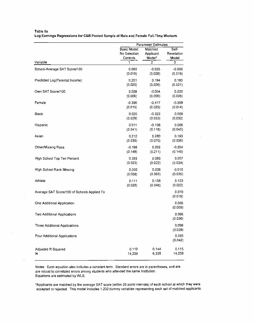
Table 5aLog Earnings Regressions for C&B Pooled Sample of Male and Female Full-Time Workers

Parameter EstimatesBasic Model: Matched Self-No Selection Applicant Revelation

Controls Model ModelVariable 1 2 3

School-Average SAT Score/i 00 0.060 -0.025 -0.009

(0.016) (0.028) (0.019)

Predicted Log(Parerital Income) 0.201 0.194 0.180

(0.020) (0.026) (0.021)

Own SAT Score/i 00 0.028 -0.004 0.020

(0.006) (0.006) (0.005)

Female -0.396 -0.417 -0.389

(0.015) (0.025) (0.014)

Black 0.020 -0.023 0.009

(0.029) (0.053) (0.030)

Hispanic 0.011 -0.106 0.006

(0.041) (0.118) (0.045)

Asian 0.212 0.280 0.193

(0.035) (0.070) (0.036)

Other/Missing Race -0.198 0.202 -0.204

(0.148) (0.211) (0.145)

High School Top Ten Percent 0.055 0.093 0.057

(0.023) (0.022) (0.024)

High School Rank Missing 0.000 0.036 -0.010

(0.038) (0.060) (0.035)

Athlete 0.111 0.138 0.103

(0.025) (0.048) (0.022)

Average SAT Score/i 00 of Schools Applied To 0.079

(0.016)

One Additional Application 0.055

(0.009)

Two Additional Applications 0.066

(0.026)

Three Additional Applications 0.096

(0.039)

Four Additional Applications 0.093

(0.042)

AdjustedRSquared 0.110 0.144 0.115N 14,239 6,335 14,239

Notes: Each equation also includes a constant tern,. Standard errors are in parentheses, and areare robust to correlated errors among students who attended the same institution.Equations are estimated by WLS.

*Applicants are matched by the average SAT score (within 25 point intervals) of each school at which they wereaccepted or rejected. This model includes 1232 dummy variables representing each set of matched applicants.

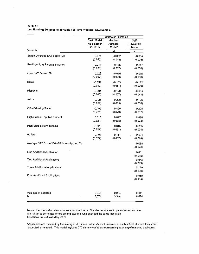
Table 5bLog Earnings Regression for Male Full-Time Workers, C&B Sample

Parameter EstimatesBasic Model: Matched Self-No Selection Applicant Revelation

Controls ModeI ModelVariable 1 2 3

School-Average SAT Score/i 00 0.071 -0.002 -0.004

(0.020) (0.044) (0.025)

Predicted Log(Parental Income) 0.241 0.176 0.217

(0.031) (0.067) (0.030)

Own SAT Score/i 00 0.026 -0.010 0.016(0.007) (0.020) (0.006)

Black -0.099 -0.183 -0.112

(0.040) (0.087) (0.039)

Hispanic -0.004 -0.170 -0.004

(0.043) (0.157) (0.041)

Asian 0.126 0.239 0.105

(0.059) (0.085) (0.060)

Other/Missing Race -0.195 0.450 -0.208

(0.271) (0.373) (0.267)

High School Top Ten Percent 0.016 0.077 0.020

(0.021) (0.035) (0.023)

High School Rank Missing -0.025 0.013 -0.035

(0.027) (0.061) (0.024)

Athlete 0.107 0.111 0.094

(0.027) (0.037) (0.024)

Average SAT Score/i 00 of Schools Applied To 0.088

(0.023)

One Additional Application 0.061

(0.015)Two Additional Applications 0.043

(0.019)Three Additional Applications 0.119

(0.030)

Four Additional Applications 0.060

(0.034)

Adjusted R Squared 0.043 0.094 0.051N 8,674 3,544 8,674

Notes: Each equation also includes a constant term. Standard errors are in parentheses, and areare robust to correlated errors among students who attended the same institution.Equations are estimated by WLS.

*Applicants are matched by the average SAT score (within 25 point intervals) of each school at which they wereaccepted or rejected. This model includes 770 dummy variables representing each set of matched applicants.

Table 6The Effect of School-Average SAT Score on Earnings in Models that Use AlternativeSelection Controls, C&B Pooled Sample of Male and Female Full-Time Workers

Type of SelectionControl

Parameter Estimates

School-AverageSAT Score

SelectionControl N

(1) None (Basic Model) 0.060

(0.016)

- 14239

(2) Average SAT Score/i 00 of Schools

Applied to (Self-Revelation Model)-0.009

(0.019)

0.079

(0.016)

14239

(3) Average SAT Score/I 00of Schools Accepted by

-0.008

(0.022)

0.073

(0.021)

14239

(4) Highest SAT Score/i 00 of

Schools Accepted by-0.014

(0.023)

0.081

(0.024)

14239

(5) Highest SAT Score/i 00 ofAll Schools Applied to

0.002

(0.018)

0.077

(0.015)14,239

(6) Highest SAT Score/i 00 of SchoolsApplied to but not Attended

0.029

(0.015)

0.047

(0.006)9,358

(7) Average SAT Score/I 00 of Schools

Rejected by

0.039

(0.014)

0.081

(0.014)3,805

(8) Highest SAT Score/I 00 of SchoolsAccepted by but not Attended

0.025

(0.015)

0.043

(0.010)8,257

Notes: Each model also includes the same control variables as the Self-Revelation Model shownin column 3 of Table 5a. Standard errors are in parentheses and are robust to correlatederrors among students who attended the same institution. Equations are estimated by WLS.The first data column presents the coefficient on the average SAT score at the school the studentattended; the second data column presents the coefficient on the selection control described inthe left margin of the table.

Table 7

Means, Standard Deviations, and Log Earnings Regressions for NLS-72 Pooled Sample of Male and Female Workers

Parameter EstimatesVariable Means Basic Model: Self-Revelation

[Standard Deviation] No Selection Controls ModelVariable Name 1 2 3

School-Average SAT Score/I 00 9.943 0.051 0.013[1.181] (0.010) (0.023)

Log(Parental Income) 9.455 0.081 0.074[0.615] (0.018) (0.018)

Own SAT Score/I 00 9.755 0.022 0.020[2.057] (0.006) (0.006)

Female 0.398 -0.384 -0.384[0.489] (0.022) (0.022)

Black 0.060 0.065 0.053[0.238] (0.047) (0.047)

Hispanic 0.016 0.096 0.085[0.124] (0.084) (0.084)

Asian 0.010 -0.175 -0.167[0.099] (0.103) (0.103)

Other/Missing Race 0.023 -0.525 -0.503[0.151] (0.069) (0.069)

High School Top Ten Percent 0.201 0.055 0.063[0.401] (0.029) (0.030)

High School Rank Missing 0.193 0.039 0.040[0.394] (0.027) (0.027)

Average SAT Score/i 00 of Schools Applied To 9.996 0.034[1.114] (0.025)

One Additional Application 0.246 0.026[0.4311 (0.025)

Two Additional Applications 0.202 0.107[0.402] (0.028)

Three Additional Applications 0.008 0.010[0.089] (0.115)

Adjusted R Squared --- 0.199 0.205N 2127 2127 2,127

Notes: Each equation also includes a constant term. Standard errors are in parentheses. Equations are estimated by WLS.All respondents who earned over $5000 in 1985 are included, regardless of full-time work status.The mean of the dependent variable is 10.087, and the standard deviation is .525.

Table 8Log Earnings Regression Allowing the Effect of School-Average SAT to Vary with Parental Income,C&B Pooled Sample of Male and Female Full-Time Workers

Parameter EstimatesBasic Model: Matched Self-No Selection Applicant Revelation

Controls Model* ModelVariable 1 2 3

School-Average SAT Score/i 00 0.660 0.654 0.573(0.226) (0.256) (0.230)

Predicted Log(Parental Income) 0.871 0.964 0.830(0.255) (0.278) (0.258)

Predicted Log of Parental lncome*School SAT Score/i 00 -0.060 -0.068 -0.058(0.023) (0.026) (0.023)

Own SAT ScoreIlOO 0.029 -0.004 0.021

(0.005) (0.006) (0.005)

Female -0.395 -0.416 -0.388(0.014) (0.025) (0.013)

Black 0.017 -0.027 0.006

(0.030) (0.052) (0.030)

Hispanic -0.001 -0.115 -0.005(0.042) (0.118) (0.046)

Asian 0.209 0.279 0.190

(0.034) (0.071) (0.036)

Other/Missing Race -0.198 0.196 -0.203(0.147) (0.210) (0.144)

High School Top Ten Percent 0.055 0.094 0.058

(0.024) (0.022) (0.024)

High School Rank Missing 0.003 0.039 -0.006(0.038) (0.061) (0.035)

Athlete 0.113 0.139 0.105

(0.024) (0.048) (0.022)

Average SAT Score/i 00 of Schools Applied To 0.079

(0.016)

One Additional Application 0.055

(0.009)

Two Additional Applications 0.065

(0.026)

Three Additional Applications 0.095

(0.039)Four Additional Applications 0.094

(0.041)

Adjusted RSquared 0.109 0.146 0.114N 14,239 6,335 14,239

Notes: Each equation also includes a constant term. Standard errors are in parentheses, andare robust to correlated errors among students who attended the same institution. Equations areestimated by WLS.

*Applicants are matched by the average SAT score (within 25 point intervals) of each school at which they wereaccepted or rejected. This model includes 1,232 dummy variables representing each set of matched applicants.

Table 9

Log Earnings Regressions using Net Tuition as School Quality Indicator, C&B Pooled Sample of Male andFemale Full-Time Workers

Parameter EstimatesBasic Models: Matched Applicant Self-Revelation

No Selection ControlsVariable 1 2

Models*3 4 5

Models6

Log(NetTuition) 0.100 0.722 0.059 1.021 0.050 0.792(0.016) (0.322) (0.031) (0.409) (0.019) (0.319)

Predicted Log(Parental Income) 0.192 0.646 0.190 0.902 0.176 0.718(0.020) (0.242) (0.025) (0.317) (0.021) (0.247)

Log(Net Tuition)*Predicted Log (Parental Income) -0.062 -0.097 -0.075(0.033) (0.043) (0.033)

Own SAT Score/i 00 0.029 0.029 -0.005 -0.005 0.019 0.019(0.005) (0.005) (0.006) (0.006) (0.005) (0.005)

Female -0.392 -0.390 -0.417 -0.416 -0.392 -0.390(0.013) (0.013) (0.024) (0.024) (0.014) (0.014)

Black 0.030 0.031 -0.025 -0.029 0.004 0.004(0.027) (0.028) (0.052) (0.052) (0.028) (0.029)

Hispanic 0.005 -0.001 -0.117 -0.127 -0.010 -0.018(0.039) (0.040) (0.116) (0.117) (0.045) (0.046)

Asian 0.206 0.204 0.275 0.274 0.186 0.184(0.031) (0.031) (0.070) (0.070) (0.035) (0.036)

Other/Missing Race -0.188 -0.187 0.212 0.206 -0.202 -0.201

(0.147) (0.147) (0.210) (0.209) (0.147) (0.147)

High School lop Ten Percent 0.067 0.068 0.098 0.100 0.062 0.063(0.027) (0.028) (0.021) (0.021) (0.027) (0.027)

High School Rank Missing -0.002 -0.001 0.041 0.044 -0.008 -0.006(0.035) (0.035) (0.060) (0.060) (0.035) (0.034)

Athlete 0.114 0.115 0.137' 0.136 0.097 0.098(0.025) (0.024) (0.048) (0.048) (0.022) (0.022)

Average SAT Score/i 00 of Schools Applied To 0.053 0.055(0.010) (0.010)

One Additional Application 0.047 0.046

(0.008) (0.007)

Two Additional Applications 0.052 0.052

(0.024) (0.024)

Three Additional Applications 0.082 0.082

(0.036) (0.036)

Four Additional Applications 0.082 0.084

(0.044) (0.043)

AdjustedRSquared 0.112 0.112 0.146 0.147 0.115 0.115N 14,239 14,239 6,335 6,335 14,239 14,239

Notes: Each equation also includes a constant term. Standard errors are in parentheses, andare robust to correlated errors among students who attended the same institution.Equations are estimated by WLS. Net tuition is average tuition minus average aid (see text).

*Applicants are matched by the average SAT score (within 25 point intervals) of each school at which they wereaccepted or rejected. This model includes 1,232 dummy variables representing each set of matched applicants.

Table 10

Linear Probability Models for Class Rank, Graduation Probability, and Advance Degree Attainment; C&B Pooled Sample of Men and Women

Dependent VanablePercentile Rank in Class Graduation (1 =yes; 0=no) Advanced Degree (1 ye5. 0=no)

Basic Model: Matched Self- Basic Model: Matched Self- Basic Model: Matched Self-No Selection Applicant Revelation No Selection Applicant Revelation No Selection Applicant Revelation

ControlsVariable 1

Modet Model Controls ModeF Model Controls Model Model2 3 4 5 6 7 8 9

School-Average SAT Score/ISO -5.636 -7.825 -6.404 0.002 -0.016 0.007 0.069 -0.002 0.035(0.661) (0.636) (0.923) (0.015) (0.015) (0.018) (0.007) (0.013) (0.011)

Predicted Log(Parental Income) 4.566 2.677 4.689 0.046 0.040 0.048 0.126 0.086 0.117(1.333) (0.946) (1.156) (0.008) (0.018) (0.009) (0.022) (0.019) (0.021)

Own SAT Score/100 5.914 5.958 5.841 0.024 0.026 0.025 0.052 0.051 0.048(0.375) (0,517) (0.391) (0.006) (0.005) (0.006) (0.007) (0.004) (0.007)

Female 7.795 8.616 7.735 0.000 -0.007 -0.001 -0.067 -0.067 -0.064(0.705) (1.138) (0.702) (0.009) (0.010) (0.009) (0.009) (0.010) (0.009)

Blach -11.375 -12.571 -11.359 -0.009 0.034 -0.008 0.131 0.127 0.126(1.649) (1.867) (1.650) (0.021) (0.038) (0.021) (0.027) (0.028) (0.027)

Hispanic -3.510 -6,388 -3.527 -0.067 -0.111 -0.068 0.106 0.077 0,103(3.395) (3.749) (3.223) (0.031) (0.076) (0.031) (0,054) (0.062) (0.055)

Asian• -0.054 -3.309 -0,108 . 0.027 0.027 0.028 0,087 0.137 0.079(2.770) (1.861) (2.661) (0.017) (0.029) (0.017) (0.026) (0.053) (0.024)

Other/Missing Race -10.957 -10.525 -11.216 -0.193 -0.177 -0.192 -0.062 -0.229 -0.064(2.148) (2.801) (2.175) (0.074) (0.151) (0.073) (0.031) (0.047) (0.032)

High School Top Ten Percent 9.566 9.753 9.322 0.050 0.028 0.051 0.072 0.064 0071(1.343) (1.637) (1.382) (0.009) (0.016) (0.009) (0.017) (0.031> (0.018)

High School Rank Missing 3.711 3.262 3.655 0,045 0.015 0.047 0.018 0.019 0.014(0.912) (1.059) (0.927) (0.016) (0.017) (0.015) (0.017) (0.029) (0.019)

Athlete -1.293 -1.592 -1.103 0.063 0.022 0.063 0.006 0.008 0.004(0.818) (1.798) (0.867) (0.014> (0.012) (0.013) (0.019) (0.029) (0.019)

Average SAT Score/lOU of Schools Applied To 1,681 -0.007 0.043(0.841) (0.005) (0.012)

One Additional Application 0.052 0.015 0.018(0.640) (0.012) (0.011)

Two Additional Applications -1.436 0.015 0.034(0.843) (0.009) (0.013)

Three Additional Applications -4,009 0.006 0.013

(0.863) (0.015> (0.020)

Four Additional Applications -7,507 -0.064 -0.002(1.344) (0.022) (0.020)

Adjusted R Squared 0.181 0.232 0.185 0.023 0.099 0.024 0.087 0.120 0.089N . 19,062 9,042 19,062 19,505 9.207 19,505 19.505 9,207 19,505

Notes: Sample includes all survey respondents, regardless of full-time work status. The percentile rank in class regression excludes those who were missing gradepoint averages. The graduation regression counts as graduates only those students who graduated from the same C&B school at which they first matriculated.Each equation also includes a constant term. Standard enore are in parentheses, and are robust to correlated errors among students whoattended the same institution. Equations are estimated by WLS.

Applicants are matched by the average SAT score (within 25 point intervals> of each school at which they wereaccepted or rejected. This model indudes 1.566 dummy variables representing each set of matched applicants.

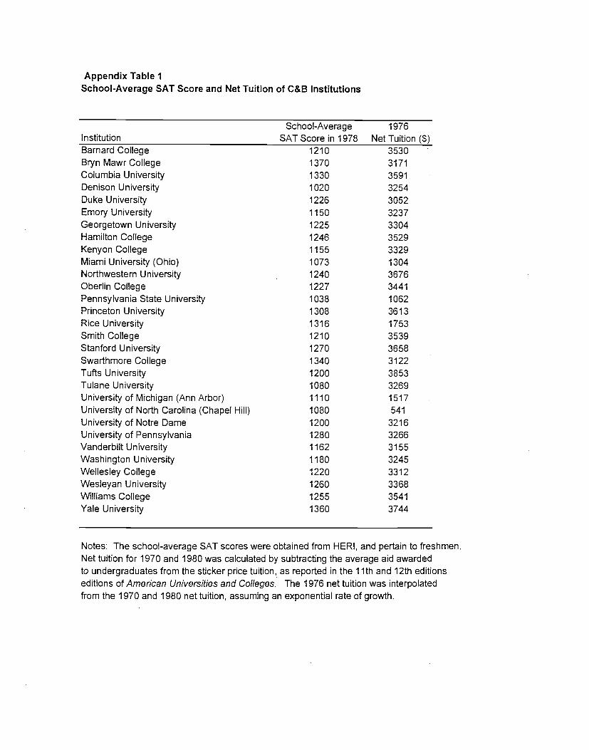
Appendix Table ISchool-Average SAT Score and Net Tuition of C&B Institutions

School-Average 1976Institution SAT Score in 1978 Net Tuition ($)Barnard College 1210 3530Bryn Mawr College 1370 3171Columbia University 1330 3591Denison University 1020 3254Duke University 1226 3052Emory University 1150 3237

Georgetown University 1225 3304Hamilton College 1246 3529

Kenyon College 1155 3329

Miami University (Ohio) 1073 1304Northwestern University 1240 3676Oberlin College 1227 3441

Pennsylvania State University 1038 1062

Princeton University 1308 3613Rice University 1316 1753Smith College 1210 3539Stanford University 1270 3658Swarthmore College 1340 3122Tufts University 1200 3853Tulane University 1080 3269

University of Michigan (Ann Arbor) 1110 1517

University of North Carolina (Chapel Hill) 1080 541University of Notre Dame 1200 3216

University of Pennsylvania 1280 3266Vanderbilt University 1162 3155

Washington University 1180 3245

Wellesley College 1220 3312

Wesleyan University 1260 3368Williams College 1255 3541

Yale University 1360 3744

Notes: The school-average SAT scores were obtained from HERI, and pertain to freshmen.Net tuition for 1970 and 1980 was calculated by subtracting the average aid awardedto undergraduates from the sticker price tuition, as reported in the 11th and 12th editionseditions of American Universities and Colleges. The 1976 net tuition was interpolatedfrom the 1970 and 1980 net tuition, assuming an exponential rate of growth.

Appendix Table 2Regression Predicting the Natural Log of Parental Income, C&B Sample

Parameter StandardVariable Estimate ErrorYears of Father's Education 0.067 0.003Years of Mothers Education 0.031 0.003Mothers Education Missing 0.550 0.096Fathers Education Missing 0.915 0.085Fathers Occupation Missing*Fathers Education 0.015 0.004Mothers Occupation MissingMother's Education 0.007 0.005Father Clerical Occupation 0.567 0.097Father Management Consultant 0.678 0.168Father Sales 0.669 0.044Father Social Work 0.563 0.283Father Communications 0.790 0.129Father Policeman 0.503 0.182Father Financial Services 0.813 0.048Father Engineer 0.808 0.042Father Computer Occupation 0.564 0.154Father Physician 0.839 0.047Father Religious Worker 0.132 0.069Father Social Sciences 0.695 0.096Father Primary or Secondary Teacher 0.549 0.047Father Post-Secondary Teacher 0.466 0.050Father Writer, Arts, etc. 0.670 0.063Father Top Government position 0.897 0.220Father Lawyer or Judge 0.819 0.049Father Health Occupation .

0.640 0,054Father Math or Science Occupation 0.678 0.059Father Military 0.531 0,056Father Service Occupation 0.521 0.061Father Agriculture 0.333 0.062Father Businessman (general) 0.752 0.043Father Other Occupation 0.606 0.042Father Management Occupation 0.886 0.040Father Skilled Worker 0.577 0.045Father Semi-skilled Worker 0.409 0.050Father Unskilled Worker 0.339 0.063Fathers Occupation Missing 0.376 0.082Mother Clerical Occupation -0.098 0.019Mother Management Consultant -0.393 0.654Mother Sales -0.090 0.039Mother Social Work 0.032 0.118Mother Communications 0.009 0.142Mother Policeman 0.388 0.341Mother Financial Services -0.004 0.054Mother Engineer -0.078 0.188Mother Computer Occupation 0.149 0.222Mother Physician 0.061 0.097Mother Religious Worker -0.477 0.180Mother Social Sciences -0.031 0.071Mother Primary or Secondary Teacher -0.045 0.019Mother Post-Secondary Teacher -0.062 0.055Mother Writer. Arts, etc. -0.125 0.039Mother Top Government Position 0.077 0.308Mother Lawyer or Judge -0.018 0.168Mother Health Occupation -0.081 0.023Mother Math or Science Occupation -0.004 0.150Mother Service Occupation -0.201 0.069Mother Agriculture -0.043 0.281Mother Business (general) 0.008 0.053Mother Other Occupation -0.077 0.019Mother Management Occupation 0.025 0.038Mother Skilled Worker -0.140 0.052Mother Semi-skilled Worker -0.176 0.039Mother Unskilled Worker -0.299 0.070Mothers Occupation Missing -0.054 0,08 1

R Squared 0.342N 10,525

Notes: Baseline categories are "father not working" and "mother not working.' The equation also includes a constant term.The primary source of parental occupation is the C&B institutional file, which is based on students' college applications.Parental Income information is from responses to the Student Descriptive Questionnaire (SDQ), administered by theEducational Testing Service (ETS) when the students took the SAT. Mother's and father's education are basedon responses to the C&B survey: "During your senior year in high school, what was the highest level of educationyour mother (father) had attained?" Students' responses to the CIRP freshmen questionnaire were used to fill in parentaloccupation and education if these variables were unavailable from the other sources.