Embed Size (px)
Citation preview
NAZAROV-WENZL ALGEBRAS, COIDEAL SUBALGEBRAS
AND CATEGORIFIED SKEW HOWE DUALITY
MICHAEL EHRIG AND CATHARINA STROPPEL
Abstract. We describe how certain cyclotomic Nazarov-Wenzl alge-bras occur as endomorphism rings of projective modules in a parabolicversion of BGG category O of type D. Furthermore we study a fam-ily of subalgebras of these endomorphism rings which exhibit similarbehaviour to the family of Brauer algebras even when they are notsemisimple. The translation functors on this parabolic category O arestudied and proven to yield a categorification of a coideal subalgebra ofthe general linear Lie algebra. Finally this is put into the context ofcategorifying skew Howe duality for these subalgebras.
Contents
Introduction 11. Basics 52. Brauer and VW-algebra 73. Isomorphism theorem 164. Cyclotomic quotients 285. Koszulness and Gradings 366. Coideal subalgebras 377. Skew Howe duality 518. Appendix 63References 68
Introduction
In [BK09] a remarkable connection between the representation theory ofHecke algebras and Lusztig’s canonical bases was established by showingthat cyclotomic Hecke algebras are isomorphic to cyclotomic quotients ofquiver Hecke algebras introduced in [KL09], [KL08], where also a connectionbetween the representation theory of these algebras and Lusztig’s geometricconstruction of canonical bases was predicted. This prediction was verified,
Key words and phrases. category O, coideal algebras, Kazhdan-Lusztig polynomials,categorification, skew Howe duality.
M.E. was financed by the DFG Priority program 1388. This material is based on worksupported by the National Science Foundation under Grant No. 0932078 000, while theauthors were in residence at the MSRI in Berkeley, California.
1
2 MICHAEL EHRIG AND CATHARINA STROPPEL
[VV11], and so therefore a connection between representations of cyclotomicHecke algebras and canonical bases was established. In this way, cyclotomicHecke algebras inherit an interesting grading which in type A can also beobtained from the graded versions of parabolic category O’s and hence bedescribed in terms of type A Kazhdan-Lusztig polynomials, see [BS11b],[HM11]. In other types however, Schur-Weyl duality connects the Lie al-gebra with a centralizer algebra (Brauer algebra) different from the groupalgebra of any Weyl group. In this paper we investigate relations betweenparabolic category Op(so2n), Brauer algebras and their degenerate affineversions ⩔d =⩔d(Ξ), depending on a parameter set Ξ, and their cyclotomicquotients, [AMR06]. The algebras ⩔d(Ξ) were introduced in [Naz96] basedon work of Wenzl, we call them therefore VW-algebra an abbreviation of theGerman ‘verallgemeinerte Wenzl algebra’.1 These families are the Braueralgebra analogues of the cyclotomic Hecke algebras, but in contrast to themnot well understood and so far slightly neglected; maybe also because ofthe lack of a good combinatorial description and geometric realization. Themain goal of the paper is to connect these algebras to category O and itsKazhdan-Lusztig combinatorics and in this way obtain canonical bases ofrepresentations for coideal subalgebras in quantum groups.
We start with a type D analogue of the Arakawa-Suzuki theorem:
Theorem A. Let M be a highest weight module in O(so2n). With anappropriate choice of Ξ there is an algebra homomorphism
ΨM ∶ ⩔d Ð→ Endg(M ⊗ (C2n)⊗d
)opp.
In general this morphism is not surjective and it is impossible to describethe kernel. We study in detail the case where M is a parabolic Verma moduleMp(λ) for a maximal parabolic subalgebra of type A inside type D. We showthat cyclotomic quotients ⩔d(α,β) of level 2 occur as endomorphism ringsif we choose λ = δω0 as an appropriate multiple of a fundamental weight:
Theorem B (see Theorem 3.1). If n ≥ 2d and δ ∈ Z then
⩔d(α,β) ≅ Endg(Mp(δ)⊗ (C2n
)⊗d
)opp.
We deduce that the ⩔d(α,β)’s inherit a positive Koszul grading from the
graded version O, of category O, hence a geometric interpretation; in termsof first perverse sheaves on isotropic Grassmannians, [ES13b], and secondtopological Springer fibres, [ES12], via the Khovanov algebra of typeD. ThisKhovanov algebra also allows us, [ES13a], to mimic (with some effort) theapproach from [BS12] to construct a graded version of the Brauer algebraBr(δ) for an arbitrary integral parameter δ. Since this requires passingto orthosymplectic Lie superalgebras, we just identify here a subalgebrazd⩔d(α,β)zd of the cyclotomic quotient, given by an idempotent zd andshow that this algebra shares properties of the Brauer algebra:
1Keeping in mind that VW can be seen as a degeneration of BMW, the affine Birman-Murakawi-Wenzl algebras.
NAZAROV-WENZL ALGEBRAS AND SKEW HOWE DUALITY 3
Theorem C (see Proposition 4.4 and Theorem 4.5). .
(1) The algebra zd⩔d(α,β)zd has dimension (2d − 1)!!.(2) The algebra zd⩔d(α,β)zd is semisimple if and only if δ /= 0 and
δ ≥ d − 1 or δ = 0 and d = 1,3,5.
These connections give a conceptual explanation for the fact, [CDVM09b]and [CDVM09a], that the decomposition numbers of Brauer algebras aregiven by the combinatorics of Weyl groups of type D.
Theorems A and B and [ES13a] rely on a good understanding of (a gradedversion of) tensoring with the natural representation C2n on category Op.Since C2n is self-dual and hence ⊗ C2n self-adjoint, we do not get an ac-tion of a quantum group action on our categories, but rather of certaincoideal subalgebras H and H of Uq(glZ) so-called quantum symmetric pairsin [Let03], [Let02], [Kol12]. These are quantum group analogues of the fixedpoint subalgebra glN ×gl−N inside glZ. Since the integral weights of so2n canbe partitioned into integer or half-integer weights in the standard ε-basis,the integral part, Op(so2n), of parabolic category O can be decomposed intotwo subcategories Op
1(so2n) and Op (so2n) stable under tensoring with the
natural representation. We obtain two categorifications
Theorem D (see Proposition 6.25).
(1) The H-module ⋀nCZ is categorified by Op1(so2n).
(2) The H -module ⋀nCZ+ 12 is categorified by Op
(so2n).
The classes of Verma modules correspond hereby to the standard basis.The involved categories have a contravariant duality, hence the categori-fication equips the modules on the left with a bar-involution, see Propo-sition 6.30. Mimicking Lusztig’s approach for quantum groups, we definecanonical bases on the above modules and show that the classes of simplemodules correspond to the canonical basis. Theorem D gives a new instanceof based categorifications in the context of category O, but now connectingcanonical bases of Hecke algebras with canonical bases of quantum sym-metric pairs instead of quantum groups as for instance in [BS10], [FKS06],[Sar13], [Web10], see [Maz12] for an overview. The base change matrix ishere given by parabolic type D Kazhdan-Lusztig polynomials; see [LS13] forexplicit formulas in the Grassmannian case.
Finally we investigate generalizations of these modules from the viewpointof skew Howe duality, [How92], and its categorification. For this we considermore general parabolic category O’s and their block decompositions for Levisubalgebras isomorphic to products of glk’s. Denote the sum of these blocksby ⊕ΓOΓ(n). Considering analogous projective functors in this setup wecategorify the two actions of glm × glm and glr × glr on the vector space
⋀(n,m, r) ∶= ⋀n(Cm ⊗ C2 ⊗ Cr) separately and then show they are gradedderived equivalent via Koszul duality. Under this identification we can real-ize both commuting actions on the same category. The projective functorsturn into derived Zuckerman functors under this identification.
4 MICHAEL EHRIG AND CATHARINA STROPPEL
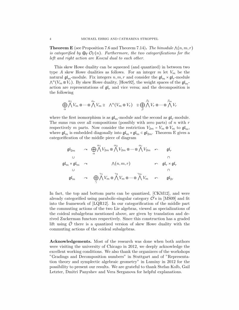
Theorem E (see Proposition 7.6 and Theorem 7.14). The bimodule ⋀(n,m, r)is categorified by ⊕ΓOΓ(n). Furthermore, the two categorifications for theleft and right action are Koszul dual to each other.
This skew Howe duality can be squeezed (and quantized) in between twotype A skew Howe dualities as follows. For an integer m let Vm be thenatural glm-module. Fix integers n,m, r and consider the glm × glr-module
⋀n(Vm⊗Vr). By skew Howe duality, [How92], the weight spaces of the glm-
action are representations of glr and vice versa; and the decomposition isthe following
⊕α
α1
⋀Vm ⊗⋯⊗αr
⋀Vm ≅ ⋀n(Vm ⊗ Vr) ≅⊕
β
β1
⋀Vr ⊗⋯⊗βm
⋀ Vr
where the first isomorphism is as glm-module and the second as glr-module.The sums run over all compositions (possibly with zero parts) of n with rrespectively m parts. Now consider the restriction V2m = Vm ⊕ Vm to glm,where glm is embedded diagonally into glm × glm ⊂ gl2m. Theorem E gives acategorification of the middle piece of diagram
gl2m ⊕α
α1
⋀V2m ⊗α2
⋀V2m ⊗⋯⊗αr
⋀V2m glr
∪ ∩
glm × glm ⋀(n,m, r) glr × glr
∪ ∩
glm ⊕γ
γ1
⋀Vm ⊗γ2
⋀Vm ⊗⋯⊗γ2r
⋀ Vm gl2r
In fact, the top and bottom parts can be quantized, [CKM12], and werealready categorified using parabolic-singular category O’s in [MS09] and fitinto the framework of [LQR12]. In our categorification of the middle partthe commuting actions of the two Lie algebras, viewed as specializations ofthe coideal subalgebras mentioned above, are given by translation and de-rived Zuckerman functors respectively. Since this construction has a gradedlift using O there is a quantized version of skew Howe duality with thecommuting actions of the coideal subalgebras.
Acknowledgements. Most of the research was done when both authorswere visiting the university of Chicago in 2012, we deeply acknowledge theexcellent working conditions. We also thank the organizers of the workshops”Gradings and Decomposition numbers” in Stuttgart and of ”Representa-tion theory and symplectic algebraic geometry” in Luminy in 2012 for thepossibility to present our results. We are grateful to thank Stefan Kolb, GailLetzter, Dmitri Panyshev and Vera Serganova for helpful explanations.
NAZAROV-WENZL ALGEBRAS AND SKEW HOWE DUALITY 5
1. Basics
Throughout this paper let g denote the Lie algebra so2n defined overthe complex numbers. We denote by U(g) its enveloping algebra and byZ(U(g)) the center of U(g). In Section 2 we will fix a specific presentationfor so2n.
We denote by εi the standard basis of the dual of the Cartan h∗ withsimple roots αi = εi+1 − εi for 1 ≤ i ≤ n − 1 and α0 = ε1 + ε2. By abuse ofnotation we denote by O the sum of all integral blocks of the BGG-categoryO of g. We fix the maximum standard parabolic p of type A correspondingto the roots α1, . . . , αn−1 and denote the associated parabolic subcategoryof O by Op(n), i.e. the subcategory of O of all p-finite modules. Thecombinatorics of this parabolic subcategory was studied in [ES13b] and werecall some of the notations used therein.
A weight λ = (λ1, . . . , λn) ∈ h∗ of so2n is integral if it is in the Z-span or
the (Z+ 12)-span of the εi’s. In the former case we say the weight is supported
on the integers, in the latter that it is supported on the half-integers.For λ ∈ h∗ let Mp(λ) denote the parabolic Verma module of highest weight
λ, that is the maximal quotient of the ordinary Verma module M(λ) whichis locally p-finite. Explicitly, Mp(λ) = 0 if λ is not p-dominant and otherwise
Mp(λ) = U(g)⊗U(p) E(λ) (1)
where E(λ) denotes the finite dimensional l-module of highest weight λfor the Levi subalgebra l of p inflated trivially to a p-module. The set ofp-dominant weights will be denoted by
Λ = λ ∈ h∗ integral ∣Mp(λ) /= 0
= λ ∈ h∗ integral ∣ λ =n
∑i=1
λiεi where λ1 ≤ λ2 ≤ ⋯ ≤ λn
= λ ∈ h∗ integral ∣ λ + ρ =n
∑i=1
λ′iεi where λ′1 < λ′2 < ⋯ < λ′n . (2)
where ρ denotes the half-sum of positive roots, ρ = ∑ni=1(i − 1)εi or ρ =
(0,1,2, . . . , n−1) in the ε-basis. It decomposes into a disjoint union Λ1 ∪Λ ,the weights supported on the integers and those supported on half-integers.Since up to the last section we only work with parabolic Verma modules, wejust call them by abuse of language for short Verma modules.
The action of the center U(g) decomposes each module into generalizedeigenspaces, which induces a decomposition O = ⊕χOχ of the category Ofor g indexed (via the Harish-Chandra isomorphism) by orbits of integralweights under the dot action w ⋅λ = w(λ+ ρ)− ρ of the Weyl group Wn of g.The decomposition of O induces a decomposition of the subcategory Op(n).We denote by Op
λ(n) the summand containing Mp(λ), i.e. the summandcorresponding to the orbit through λ + ρ. Note that the ordinary action aswell as the dot-action of the Weyl group on integral weights preserve the
6 MICHAEL EHRIG AND CATHARINA STROPPEL
lattices of weights supported on integers resp. on half-integers. Hence, wehave a decomposition
Op(n) = Op
1(n)⊕Op (n), (3)
where Op1(n) (resp. Op
(n)) is the direct sum of all Opλ(n), such that λ is
supported on the integers (resp. half-integers).Our goal is to equip the Grothendieck groups of Op
1(n) and Op (n) with
the structure of a representation of a certain coideal subalgebra induced bythe action of translation functors, see Section 6. To make this explicit itis helpful to use the combinatorics from [ES13b, Section 2.2] to identify p-dominant weights with diagrammatic weights, allowing us to describe theblocks of category Op(n) combinatorially. Since we want to distinguishthe combinatorics for the two subcategories in (3) we slightly modify theindexing sets for diagrammatic weights from [ES13b].
Definition 1.1. We denote by Xn the set of sequences a = (ai)i∈Z≥0 suchthat ai ∈ ∧,∨,×, ,, ai ≠ for i ≠ 0, a0 ∈ ,, and
#ai ∣ ai ∈ ∧,∨, + 2#ai ∣ ai = × = n.
Elements of Xn are called diagrammatic weights supported on the integers.
Remark 1.2. The translation from a diagrammatic weight a ∈ X to a di-agrammatic weight a in the sense of [ES13b] is done by setting ai = ai−1,except for i = 1 and a0 = where we choose a1 ∈ ∧,∨ such that the totalnumber of ∨’s is even. In the language of [ES13b] we have thus always fixedthe even parity for these blocks where a0 = .
Similarly we have a set-up for half-integers.
Definition 1.3. We denote by X n the set of sequences a = (ai)i∈Z≥0+ 1
2such
that ai ∈ ∧,∨,×, and #ai ∣ ai ∈ ∧,∨ + 2#ai ∣ ai = × = n. We callthese elements diagrammatic weights supported on the half-integers.
Remark 1.4. Translating a diagrammatic weight a ∈ X to a diagrammaticweight a in the sense of [ES13b] is done by putting ai = ai− 1
2.
Obviously a diagrammatic weight a is uniquely determined by the sets
P⋆(a) = i ∣ ai = ∗,
for ⋆ ∈ ∧,∨,×, ,. Given a p-dominant weight λ = (λ1, . . . , λn), denoteλ′ = (λ′1, . . . , λ
′n) = λ + ρ and let aλ be the diagrammatic weight defined by
P∨(λ) = λ′i ∣ λ′i > 0 and − λ′i does not appear in λ′,
P∧(λ) = −λ′i ∣ λ′i < 0 and − λ′i does not appear in λ′,
P×(λ) = λ′i ∣ λ′i > 0 and − λ′i appears in λ′,
P(λ) = λ′i ∣ λ′i = 0,
P(λ) = Z≥0 ∖ (P∨ ∪ P∧ ∪ P× ∪ P) if λ is supported on integers,Z≥0 +
12 ∖ (P∨ ∪ P∧ ∪ P×) if λ is supported on half-integers.
NAZAROV-WENZL ALGEBRAS AND SKEW HOWE DUALITY 7
The assignment λ ↦ aλ defines a bijection between p-dominant weightsand Xn ∪ X
n. In the following we will not distinguish between a weightand a diagrammatic weight and denote both by λ. We use the followingidentifications
K0 (Op1(n)) ≅ ⟨Xn⟩Q and K0 (O
p (n)) ≅ ⟨X
n⟩Q ,
between the Q-vector spaces on basis Xn resp. X n and the Grothendieck
group scalar extended to Q by sending the class of a parabolic Verma moduleof highest weight λ to aλ.
Our weight dictionary induces an action of the Weyl group Wn on dia-grammatic weights corresponding to the dot-action on weights for g. Twodiagrammatic weights are in the same orbit (and thus the correspondingVerma modules have the same central character) if and only if one is ob-tained from the other by a finite sequence of changes of the following form:swapping a ∨ with an ∧ or replacing two ∨’s with two ∧’s or two ∧’s with two∨’s (keeping all ×’s and ’s untouched), see [ES13b]. Orbits of diagrammaticweights, called diagrammatic blocks are given by fixing the positions of the×’s and ’s (called block diagram in [ES13b, Section 2.2]) and the parity of#∨+#× of any of its weights. Moving ∨’s to the left or turning two ∧’s intotwo ∨’s makes the weight bigger (with respect to the standard ordering onweights). Note that diagrammatic blocks correspond precisely to blocks ofOp(n) by sending Γ to the summand Op(n)Γ containing all Verma moduleswith highest weight in Γ which is indeed a block of the category.
2. Brauer and VW-algebra
2.1. VW-algebras and translated highest weight modules. The mainpurpose of this section is a generalization of the Arakawa-Suzuki action,[AS98], to the Lie algebra of type Dn. The replacement of the degenerateaffine Hecke algebra is the affine Nazarov-Wenzl algebra ⩔d(Ξ).
Definition 2.1. Let d ∈ N. We fix a set Ξ of parameters wk ∈ C, k ≥ 0.Then the affine Nazarov-Wenzl algebra ⩔d = ⩔d(Ξ), short VW -algebra, isgenerated by
si, ei, yj 1 ≤ i ≤ d − 1,1 ≤ i ≤ d, k ∈ N, (4)
subject to the relations (for 1 ≤ a, b ≤ d − 1, 1 ≤ c < d − 1, and 1 ≤ i, j ≤ d):
(VW.1) s2a = 1
(VW.2) (a) sasb = sbsa for ∣ a − b ∣> 1(b) scsc+1sc = sc+1scsc+1
(c) sayi = yisa for i /∈ a, a + 1(VW.3) e2
a = w0ea(VW.4) e1y
k1e1 = wke1 for k ∈ N
(VW.5) (a) saeb = ebsa and eaeb = ebea for ∣ a − b ∣> 1(b) eayi = yiea for i /∈ a, a + 1(c) yiyj = yjyi
8 MICHAEL EHRIG AND CATHARINA STROPPEL
(VW.6) (a) easa = ea = saea(b) scec+1ec = sc+1ec and ecec+1sc = ecsc+1
(c) ec+1ecsc+1 = ec+1sc and sc+1ecec+1 = scec+1
(d) ec+1ecec+1 = ec+1 and ecec+1ec = ec(VW.7) saya − ya+1sa = ea − 1 and yasa − saya+1 = ea − 1(VW.8) (a) ea(ya + ya+1) = 0
(b) (ya + ya+1)ea = 0
Remark 2.2. Relations (6b), (6c), (6d), (7) come in pairs and it is infact sufficient to either require the first set of relations or the second, theother is then satisfied automatically. All relations are symmetric or come insymmetric pairs, thus we have a canonical isomorphism ⩔d(Ξ) ≅⩔d(Ξ)opp.
From now on we fix a natural number n ≥ 4 and set N = 2n. Let I+ ∶=1, . . . , n and I ∶= I+ ∪ −I+. We denote by V the vector space with basisvi ∣ i ∈ I and by gl(I) its corresponding Lie algebra of endomorphisms,viewed as the matrices with respect to the chosen basis. Let J be the matrixsuch that Jkl = δk,−l for k, l ∈ I with respect to the chosen basis. If we ordercolumns and rows decreasing from top to bottom and left to right this is thematrix with ones on the anti-diagonal and zeros elsewhere.
Definition 2.3. The Lie algebra g = so2n is the Lie subalgebra of gl(I) ofall matrices A satisfying JA +AtJ = 0; that is all matrices which are skew-symmetric with respect to the anti-diagonal, Ai,j = −A−j,−i. In terms of thebilinear form ⟨−,−⟩ on V defined by J we thus have ⟨Xv,w⟩ + ⟨v,Xw⟩ = 0.
Fix the Cartan subalgebra h ⊂ g given by all diagonal matrices and a basisεi ∣ i ∈ I
+ for h∗ such that the weight of vi is εi if i ∈ I+ and the weight of vi is−εi if i ∈ I−. For any α ∈ Rn = R(so2n) = ±εi±εj ∣ i ≠ j fix a root vector Xα
of weight α and for i ∈ I+ let Xi be the element in h dual to εi. Then Xγ ∣ γ ∈
Bn with Bn = Rn ∪ I+ form a basis of so2n. We set n+ = ⟨Xεi±εj ∣ i > j⟩, and
n− = ⟨X−(εi±εj) ∣ i > j⟩ and fix the Borel subalgebra b = n+⊕h. In this notation
the natural representation V is the irreducible representation L(εn) withhighest weight εn, the fundamental weight corresponding to αn−1 = εn−εn−1.Furthermore, the X±(εi−εj)’s for i > j together with h form a Levi subalgebra l
isomorphic to gln with corresponding standard parabolic subalgebra p = l+n+
from Section 1.For i ∈ I denote by v∗i = v−i the basis element dual to vi with respect to
⟨−,−⟩ and for Xγ denote by X∗γ the element dual to Xγ with respect to the
Killing form of so2n.
Definition 2.4. Let M be a g-module. For d ≥ 0 consider M ⊗ V ⊗d. Thelinear endomorphisms τ, σ ∶ V ⊗ V Ð→ V ⊗ V defined as
τ ∶ v ⊗w ↦ ⟨v,w⟩∑i∈I
vi ⊗ v∗i , (5)
σ ∶ v ⊗w ↦ w ⊗ v. (6)
NAZAROV-WENZL ALGEBRAS AND SKEW HOWE DUALITY 9
induce the following endomorphisms si, ei of M ⊗ V ⊗d for 1 ≤ i ≤ d − 1
si = Id⊗ Id⊗(i−1)⊗σ ⊗ Id⊗(d−i−3), (7)
ei = Id⊗ Id⊗(i−1)⊗τ ⊗ Id⊗(d−i−3) . (8)
By definition of the comultiplication it is obvious that si is a g-homomorphismand using the compatibility of g and the bilinear form it immediately followsthat ei is as well (see also Remark 2.6), hence both are in Endg (M ⊗ V ⊗d).
Definition 2.5. The pseudo Casimir element in U(g)⊗ U(g) is defined as
Ω = ∑γ∈Bn
Xγ ⊗X∗γ . (9)
It is connected to the ordinary Casimir element C = ∑γ∈BnXγX∗γ by the
formula
Ω =1
2(∆(C) −C ⊗ 1 − 1⊗C),
where ∆ denotes the comultiplication of g. Denote by cλ the value by whichC acts on a module of highest weight λ. For 0 ≤ i < j ≤ d we define
Ωij = ∑γ∈Bn
1⊗ . . .⊗Xγ ⊗ 1⊗ . . .⊗ 1⊗X∗γ ⊗ 1⊗ . . .⊗ 1, (10)
where Xγ is at position i and x∗γ is at position j. Multiplication with Ωi,j
defines an element Ωi,j ∈ Endg(M ⊗ V ⊗d) and we finally set for i ∈ I
yi = ∑0≤k<i
Ωki + (2n − 1
2Id) , (11)
By definition of Ω it is clear that yi is a g-endomorphism on M ⊗ V ⊗d.
Remark 2.6. The representation V ⊗ V decomposes as a g-module intothe irreducible representations L(0), L(2εn), and L(εn + εn−1). A smallcomputation shows that on V ⊗ V the following equation holds
Ω = −prL(0)(cεn id + σ) + σ.
Note that τ is a quasi-projection from V ⊗ V onto the copy of the trivialrepresentation L(0) inside V ⊗ V . A small computation using the explicitform of Ω given above shows that multiplication with Ω on V ⊗ V is equalto the morphism σ − τ .
Recall that a highest weight module for g is a g-module M which is gen-erated by a non-zero vector m ∈ M satisfying n+m = 0 and hm ⊆ Cm.Note that it satisfies Endg(M) = C. Associated with λ ∈ h∗ and the corre-sponding 1-dimensional module Cλ we have the (ordinary) Verma moduleM(λ) = U(g)⊗U(b)Cλ of highest weight λ and its irreducible quotient L(λ).
Lemma 2.7. If M is a highest weight module then for each k ∈ N, thereexist ak(M) ∈ C such that e1y
k1e1 = ak(M)e1 as elements in Endg(M ⊗V ⊗d)
with a0(M) = N .
10 MICHAEL EHRIG AND CATHARINA STROPPEL
Proof. The first equality follows directly from the definitions. RecallingRemark 2.6, we first let d = 2 and consider the composition
f ∶M =M ⊗L(0)Ð→M ⊗ V ⊗ Vyk1Ð→M ⊗ V ⊗ V
e1Ð→M ⊗L(0) =M,
where the first map is the canonical inclusion. Now f is an endomorphism ofM , hence must be a multiple, say ak(M), of the identity. By pre-composingwith e1 we obtain e1y
k1e1 = ak(M)e1. This identity also holds for d > 2 since
we just add a couple of identities on the following tensor factors.
Theorem 2.8. Let M be a highest weight module for g = so2n and ΞM =
ak(M) ∣ k ≥ 0 as in Lemma 2.7. Then there is a well-defined right actionof ⩔d(2n) on M ⊗ V ⊗d defined by
p.si = si(p), p.ei = ei(p), p.yj = yj(p), p.wk = ak(M)p
for p ∈M ⊗ V ⊗d, 1 ≤ i ≤ r − 1, 1 ≤ j ≤ r and k ∈ Z. In particular, we get analgebra homomorphism
ΨM = Ψd,nM ∶ ⩔d(ΞM) Ð→ Endg(M ⊗ V ⊗d
)opp.
Proof. To prove the statement we need to show that the assignment respectsthe relations of the degenerate affine Wenzl algebra. This will be done inseparate Lemmas in the Appendix. Relation (1) is obvious, as are relations(2a) and (2b), while (2c) follows from Lemma 8.1. Relation (3) is obviousas well and relation (4) follows from Lemma 2.7. The relations (6a)-(6d)follow from Lemma 8.2, Relation (5a) is trivial as well, while (5b) followsfrom Lemma 8.4 and (5c) from Lemma 8.5. Finally relation (7) follows fromLemma 8.3 and relations (8a)-(8b) from Lemma 8.6.
As one can see from the proof of Theorem 2.8 the parameters of thedegenerate affine Wenzl algebra depend on n and the highest weight of M .This is different from the type A situation. There, the degenerate affineHecke algebra Hd acts on the endofunctor Er ∶= ⊗ V ⊗r of O(gln) for anyn, with V being the natural representation of gln. This property plays animportant role in the context of categorification of modules over quantumgroups, [KL09], [Rou08], [BK08], [BS11b]. To achieve a similar situationone could enlarge the algebra to the algebra generated by ei, si 1 ≤ i ≤ d − 1plus an extra central generator w0 subject to the same relations as beforeexcept that we have to drop relation (4). If one works with the Birman-Murakawi-Wenzl algebra instead a similar action is given in [OR07].
Remark 2.9. The action defined here can also be modified to give an actionof ⩔d(ΞM) for a highest weight module M for a Lie algebra of types B orC and the respective defining representation as V .
2.2. Brauer algebras. Let r ∈ Z≥0. A Brauer diagram on 2r vertices isa partitioning b of the set 1,2, . . . , r,1∗,2∗, . . . r∗ into r subsets of car-dinality 2. Let B[r] be the set of such Brauer diagrams. A Brauer di-agram can be displayed graphically by arranging 2r vertices in two rows
NAZAROV-WENZL ALGEBRAS AND SKEW HOWE DUALITY 11
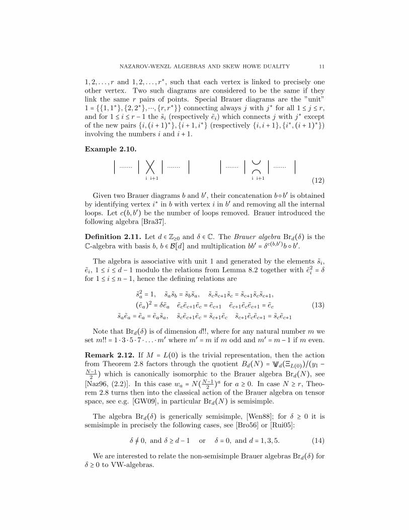
1,2, . . . , r and 1,2, . . . , r∗, such that each vertex is linked to precisely oneother vertex. Two such diagrams are considered to be the same if theylink the same r pairs of points. Special Brauer diagrams are the ”unit”1 = 1,1∗,2,2∗,⋯,r, r∗ connecting always j with j∗ for all 1 ≤ j ≤ r,and for 1 ≤ i ≤ r − 1 the si (respectively ei) which connects j with j∗ exceptof the new pairs i, (i + 1)∗,i + 1, i∗ (respectively i, i + 1,i∗, (i + 1)∗)involving the numbers i and i + 1.
Example 2.10.
i i+1 i i+1 (12)
Given two Brauer diagrams b and b′, their concatenation bb′ is obtainedby identifying vertex i∗ in b with vertex i in b′ and removing all the internalloops. Let c(b, b′) be the number of loops removed. Brauer introduced thefollowing algebra [Bra37].
Definition 2.11. Let d ∈ Z≥0 and δ ∈ C. The Brauer algebra Brd(δ) is the
C-algebra with basis b, b ∈ B[d] and multiplication bb′ = δc(b,b′)b b′.
The algebra is associative with unit 1 and generated by the elements si,ei, 1 ≤ i ≤ d − 1 modulo the relations from Lemma 8.2 together with e2
i = δfor 1 ≤ i ≤ n − 1, hence the defining relations are
s2a = 1, sasb = sbsa, scsc+1sc = sc+1scsc+1,
(ea)2 = δea ecec+1ec = ec+1 ec+1ecec+1 = ec (13)
saea = ea = easa, scec+1ec = sc+1ec sc+1ecec+1 = scec+1
Note that Brd(δ) is of dimension d!!, where for any natural number m weset m!! = 1 ⋅ 3 ⋅ 5 ⋅ 7 ⋅ . . . ⋅m′ where m′ =m if m odd and m′ =m− 1 if m even.
Remark 2.12. If M = L(0) is the trivial representation, then the actionfrom Theorem 2.8 factors through the quotient Bd(N) = ⩔d(ΞL(0))/(y1 −N−1
2 ) which is canonically isomorphic to the Brauer algebra Brd(N), see
[Naz96, (2.2)]. In this case wa = N(N−12 )a for a ≥ 0. In case N ≥ r, Theo-
rem 2.8 turns then into the classical action of the Brauer algebra on tensorspace, see e.g. [GW09], in particular Brd(N) is semisimple.
The algebra Brd(δ) is generically semisimple, [Wen88]; for δ ≥ 0 it issemisimple in precisely the following cases, see [Bro56] or [Rui05]:
δ /= 0, and δ ≥ d − 1 or δ = 0, and d = 1,3,5. (14)
We are interested to relate the non-semisimple Brauer algebras Brd(δ) forδ ≥ 0 to VW-algebras.
12 MICHAEL EHRIG AND CATHARINA STROPPEL
2.3. Cyclotomic quotients and admissibility. Recall from [AMR06, Def-inition 2.10] that the parameters wa, a ≥ 0 are admissible if they satisfy thefollowing admissibility condition
w2a+1 +1
2w2a −
1
2
2a
∑b=1
(−1)b−1wb−1w2a−b+1 = 0 (15)
Example 2.13. The values wa ∶= N(N−12 )a for a ≥ 0 from Remark 2.12 form
an admissible sequence.
Admissibility ensures the existence of a nice basis of ⩔d as follows: Fixa Brauer diagram b ∈ B[d]. By Remark 2.12 we can write it as a productof generators si, ei. Fix such an expression and consider the correspondingexpression B in the VW-algebra. More generally, given γ, η ∈ Zr≥0 and b ∈B[d] we have the monomial yγ11 y
γ22 ⋯yγdd By
η11 y
η22 ⋯yηdd ∈ ⩔d. A monomial of
this form is regular if γi /= 0 implies i is the left endpoint of a horizontal arcin b, and ηi = 0 if i∗ is the left endpoint of a horizontal arc in b, see (27).These monomials form a basis for ⩔d by [Naz96, Theorem 4.6] in case theparameters are admissible.
Given u = (u1, u2, . . . , ul) ∈ Cl we denote by ⩔d(Ξ;u) the quotient
⩔d(Ξ,u) =⩔d(Ξ)/l
∏i=1
(y1 − ui) (16)
and call it the cyclotomic VW-algebra of level l with parameters u. Undersome additional admissibility condition, [AMR06, Theorem A, Prop. 2.15],the above basis is compatible with the cyclotomic quotients:
Proposition 2.14. If the wa, a ≥ 0 are u-admissible then ⩔d(u) has di-mension ld(2d − 1)!!. The regular monomials with 0 ≤ γi, ηi < l for 1 ≤ i ≤ rform a basis B(⩔d(u)).
For the definition of u-admissibility see [AMR06, Def. 3.6]. We only needthe special example from [AMR06, Lemma 3.5]:
Example 2.15. Assume the entries of u are pairwise distinct and non-zero.Then the wa = ∑
li=1(2ui−(−1)l)uai ∏1≤j/=i≤l
ui+ujui−uj
for a ≥ 0 form a u-admissiblesequence.
2.4. The special case M =Mp(δ). In the following we study Theorem 2.8in detail in the special case where M is a specific type of parabolic Vermamodule. Recall our choice of parabolic p from Section 1.
To δ ∈ Z we associate the weight δ = δω0 = δ2 ∑
ni=1 εi, where ω0 = ∑
ni−1 εi
denotes the fundamental weight of g corresponding to α0. In particular,δ ∈ Λ and we have the Verma module Mp(δ).
Lemma 2.16. For λ ∈ Λ, Mp(λ)⊗ V has a filtration with sections isomor-phic to Mp(λ±εj) for all j ∈ I+ such that λ±εj ∈ Λ and each of these Vermamodules appearing exactly once.
NAZAROV-WENZL ALGEBRAS AND SKEW HOWE DUALITY 13
Proof. This is a standard consequence of the definition (1) and the tensoridentity; see e.g. [Hum08, Theorem 3.6].
Applying Lemma 2.16 iteratively, we obtain a bijection between Vermamodules Mp(µ) appearing as subquotients in a Verma filtration of Mp(δ)⊗V ⊗d and d-admissible weight sequences ending at µ where the latter is de-fined as follows: For fixed d ≥ 1 and δ ≥ 0 a weight µ ∈ Λ is called d-admissiblefor δ if there is a sequence
δ = λ1→ λ2
→ ⋯→ λd = µ (17)
of length d, starting at δ and ending at µ, of weights in Λ such that λi+1
differs from λi by adding precisely one weight of V , i.e. there exists j ∈ I+
such that λi+1 = λi ± εj . For instance, there are eight 2-admissible weightsequences for δ.
δ → δ − ε1 → δ − 2ε1, δ → δ − ε1 → δ − ε1 − ε2,δ → δ − ε1 → δ, δ → δ − ε1 → δ − ε1 + εn,δ → δ + εn → δ + 2εn, δ → δ + εn → δ + εn + εn−1,δ → δ + εn → δ, δ → δ + εn → δ + εn − ε1.
Proposition 2.17. There is an isomorphism of g-modules M(δ) ⊗ V ≅
M(δ − ε1) ⊕M(δ + εn). This is an eigenspace decomposition for the actionof y1. The eigenvalues are α = 1
2(1 − δ) and β = 12(δ +N − 1).
Proof. By Lemma 2.16, Mp(δ) ⊗ V has a Verma flag of length two withthe asserted Verma modules appearing. The filtration obviously splits sincethey have different central character. The Casimir C = ∑γ∈BnXγX
∗γ acts
on a highest weight module with highest weight λ by cλ = ⟨λ,λ + 2ρ⟩, seee.g. [Mus12, Lemma 8.5.3] and on the tensor product Mp(δ)⊗V as ∆(C) =
C ⊗ 1 + 1 ⊗ C + Ω0,1. Hence y1 −N−1
2 acts on the summands Mp(δ + ν),ν = −ε1, εn of Mp(δ)⊗ V by
1
2(⟨δ + ν, δ + ν + 2ρ⟩ − ⟨δ, δ + 2ρ⟩ − ⟨εn, εn + 2ρ⟩) =
⎧⎪⎪⎨⎪⎪⎩
−δ2 − (n − 1) if ν = −ε1δ2 if ν = εn
The statement follows now from the definition of α and β.
Corollary 2.18. For M = Mp(δ), the action from Theorem 2.8 factorsthrough the cyclotomic quotient with parameters (α,β) inducing an algebrahomomorphism
Ψd,nM(δ)
∶ ⩔d(ΞM(δ);α,β) Ð→ Endg(Mp(δ)⊗ V ⊗d
)opp. (18)
Definition 2.19. From now on set α = 12(1 − δ) and β = 1
2(δ +N − 1) andabbreviate ⩔d =⩔d(ΞM(δ)) and ⩔d(α,β) =⩔d(ΞM(δ);α,β).
Lemma 2.20. The elements wa, a ≥ 0 in ⩔d satisfy the recursion formulaw0 = N , w1 = N
N−12 , and for a ≥ 2
wa = (α + β)wa−1 − αβwa−2. (19)
14 MICHAEL EHRIG AND CATHARINA STROPPEL
Proof. By definition we have e1y01e1 = e
21 = Ne1, hence w0 = N . On the other
hand for any j ∈ I+ we have
e1y1e1(m⊗ vj ⊗ v∗j ) = ∑
k∈I
e1y1(m⊗ vk ⊗ v∗k)
Recalling (9), (11) this is equal to
e1∑k∈I
⎛
⎝∑i∈I+
X∗i m⊗Xivk ⊗ v
∗k + ∑
α∈Rn
Xαm⊗X∗αvk ⊗ v
∗k
⎞
⎠
+N(N − 1)
2e1m⊗ vj ⊗ v
∗j =
e1 ∑i∈I+
(∑k∈I+
X∗i m⊗ εk(Xi)vk ⊗ v
∗k − ∑
k∈I−X∗i m⊗ εk(Xi)vk ⊗ v
∗k)
+N(N − 1)
2e1m⊗ vj ⊗ v
∗j .
We obtain w1 =12(N −1)N . Finally, y2
1 = (α+β)y1−αβ by Proposition 2.17,
and hence e1yn1 e1 = (α + β)e1y
n−11 e1 − αβe1y
n−21 e1.
Lemma 2.21. The wa from Lemma 2.20 are explicitly given as
wa = Na
∑k=0
αa−k (N
2− α)
k
−N
2
a−1
∑k=0
αa−1−k(N
2− α)
k
(20)
Proof. For a = 0,1 the formula is obviously correct. Note that the recursionformula (19) has the general solution wa = Aα
a +Bβa with boundary condi-tions A +B = N and Aα +Bβ = N
2 (N − 1), see e.g. [LP98, Theorem 33.10].Hence
A =1
α − β(N
2(N − 1) −Nβ) =
1
α − β(Nα −
N
2)
and therefore
wa = N(α −1
2)αa − βa
α − β+Nβa = N(α −
1
2)a−1
∑k=0
αa−1−kβk +Nβa. (21)
The Lemma follows then by plugging in β = N2 − α.
For convenience we give a direct proof of the following result (which couldalternatively be deduced from Lemma 2.24 using [AMR06, Corollary 3.9]).
Lemma 2.22. The wa from Lemma 2.21 are admissible, i.e. satisfy (15).
Proof. Set Q(a) ∶= N ∑ak=0 αa−k (N
2 − α)k. Then wa = Q(a) − 1
2Q(a − 1) andthe admissibility condition (15) is for m = 2a + 1 equivalent to
0 = 2Q(m) −1
2Q(m − 2) +R
−m−1
∑b=1
(−1)b−1(Q(b − 1)Q(m − b) +
1
4Q(b − 2)Q(m − b − 1)) (22)
NAZAROV-WENZL ALGEBRAS AND SKEW HOWE DUALITY 15
where R = ∑m−1b=1 (−1)b−1(Q(b− 2)Q(m− b)+Q(b− 1)Q(m− b− 1)) = 0, since
Q(−1) = 0 by definition and then
R =m−1
∑b=0
(−1)bQ(b − 1)Q(m − b − 1) +m
∑b=1
(−1)b−1Q(b − 1)Q(m − b − 1)
= (−1)m−1Q(m − 1)Q(−1) +Q(−1)Q(m − 1) = 0.
By the right hand side of (22), it is enough to show that S(t) ∶= 2Q(t) −
∑tb=1(−1)b−1Q(b − 1)Q(t − b) = 0 for t = m,m − 1. For this we consider S(t)
as a polynomial in N and show that all the coefficients vanish. First notethat
2Q(t) = 2Nt
∑k=0
αt−kk
∑r=0
(k
r)
1
2rN r
(−α)k−r =t
∑k=0
k
∑r=0
(k
r)
1
2r−1(−1)k−rαt−rN r+1
Hence its coefficient in front of N s+1 equals
cs+1 =1
2s−1(−1)sαt−s
t
∑k=0
(−1)k(k
s). (23)
On the other handt
∑b=1
(−1)b−1Q(b − 1)Q(t − b) = N2t
∑b=1
(−1)b−1b−1
∑r=0
t−b
∑j=0
αb−1−r+t−b−j(N
2− α)
r+j
hence its coefficient in front of N s+1 equals
ds+1 =1
2s−1(−1)sαt−s
t
∑b=1
b−1
∑r=0
t−b
∑j=0
(−1)b+r+j(r + j
s − 1). (24)
Clearly c0 = 0 = d0 and then cs+1 = ds+1 for all s ≥ 0 by the Lemma 2.23below.
Lemma 2.23. Let m ≥ 0 be odd and s ≥ 1. Thenm
∑k=0
(−1)k(k
s) =
m
∑b=1
b−1
∑r=0
m−b
∑j=0
(−1)b+r+j(r + j
s − 1). (25)
Proof. For m = 1 the statement is clear. Let L(m) and R(m) be the left andright side of (25). We assume L(m) = R(m) and want to deduce L(m+2) =R(m+2) for which it is enough to show R(m+2)−R(m) = L(m+2)−L(m).Since m is odd, the latter is equivalent to verifying
(m + 1
s) − (
m + 2
s) = R(m + 2) −R(m) (26)
Now by definition R(m + 2) −R(m) equals
m+1
∑r=0
0
∑j=0
(−1)m+r+j(r + j
s − 1) +
m
∑r=0
1
∑j=0
(−1)m+r+j+1(r + j
s − 1)
+m
∑b=1
b−1
∑r=0
(−1)m+r+1(r +m + 1 − b
s − 1) +
m
∑b=1
b−1
∑r=0
(−1)m+r(r +m + 2 − b
s − 1)
16 MICHAEL EHRIG AND CATHARINA STROPPEL
= (−1)2m+1(m + 1
s − 1) +
m
∑r=0
(−1)m+r+2(r + 1
s − 1) +
m−1
∑r=0
(−1)m+r+1(r + 1
s − 1)
+0
∑r=0
(−1)m(m + 1
s − 1) +
m−1
∑b=1
(−1)m+b(m + 1
s − 1)
= −(m + 1
s − 1) + (
m + 1
s − 1) − (
m + 1
s − 1) − (
m + 1
s − 1)m−1
∑b=1
(−1)b
´¹¹¹¹¹¹¹¹¹¹¹¹¹¹¹¹¸¹¹¹¹¹¹¹¹¹¹¹¹¹¹¹¹¶=0
= −(m + 1
s − 1)
= (m + 1
s) − (
m + 2
s).
Lemma 2.24. The sequence wa, a ≥ 0 from Lemma 2.21 is u-admissiblefor u = (α,β).
Proof. Substituting N in formula (21) we obtain
wa =α + β
α − β(2αa+1
− 2βa+1− αa + βa)
which is easy to see to agree with the formula for wa in Example 2.15.
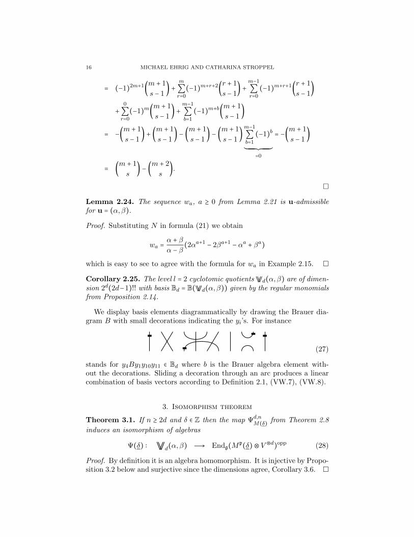
Corollary 2.25. The level l = 2 cyclotomic quotients ⩔d(α,β) are of dimen-sion 2d(2d−1)!! with basis Bd = B(⩔d(α,β)) given by the regular monomialsfrom Proposition 2.14.
We display basis elements diagrammatically by drawing the Brauer dia-gram B with small decorations indicating the yi’s. For instance
(27)
stands for y4By1y10y11 ∈ Bd where b is the Brauer algebra element with-out the decorations. Sliding a decoration through an arc produces a linearcombination of basis vectors according to Definition 2.1, (VW.7), (VW.8).
3. Isomorphism theorem
Theorem 3.1. If n ≥ 2d and δ ∈ Z then the map Ψd,nM(δ)
from Theorem 2.8
induces an isomorphism of algebras
Ψ(δ) ∶ ⩔d(α,β) Ð→ Endg(Mp(δ)⊗ V ⊗d
)opp (28)
Proof. By definition it is an algebra homomorphism. It is injective by Propo-sition 3.2 below and surjective since the dimensions agree, Corollary 3.6.
NAZAROV-WENZL ALGEBRAS AND SKEW HOWE DUALITY 17
3.1. Injectivity. We start with the proof for the injectivity.
Proposition 3.2. If n ≥ 2d and δ ∈ Z then Ψd,nM(δ)
from Theorem 2.8 induces
an injective map of algebras
Ψ(δ) ∶ ⩔d(α,β) Ð→ Endg(Mp(δ)⊗ V ⊗d
)opp (29)
Proof. By Corollary 2.25 it is enough to show that the regular monomialsyγ11 y
γ22 ⋯yγdd By
η11 y
η22 ⋯yηdd for b ∈ Bd and 1 ≤ γi, ηi < l are mapped to linearly
independent morphisms. By Remark 2.6 and (9) we have yi = Ω0,i+x, wherex is some Brauer algebra element. Let now m ∈Mp(δ) be a highest weightvector. Then Xγm = 0 for Xγ ∈ n+ and furthermore X−(εi+εj)m = 0 for all
i > j because of our specific choice of δ. (Note that E(δ) is one dimensionalin the description of Mp(δ) from (1).) Applying (9) we obtain for any a ∈ I+
Ω0,1m⊗ va =δ
2m⊗ va, Ω0,1m⊗ v−a =
δ
2m⊗ va +∑
i/=a
aiX−(εi+εj)m⊗ vi
for some ai ∈ C∗. The pm⊗ vi1 ⊗ vi2 ⊗⋯⊗ vid−1 ⊗ vid , where p runs throughall monomials in the variables X−(εi+εj) for i, j ∈ I+ with i > j form a basis
B(Mp(δ) ⊗ V ⊗d) of Mp(δ) ⊗ V ⊗d. (Note that the X−(εi+εj)’s commute due
to the structure of the root system). In particular,
yrm⊗ va =⎧⎪⎪⎨⎪⎪⎩
∑i/=ir airX−(εi+εir )vi1 ⊗⋯⊗ vir−1 ⊗ vi ⊗ vir+1 ⊗ vid + () if −a ∈ I+
() if a ∈ I+
where () stands for some linear combination of basis vectors where theabove mentioned monomials have degree zero.
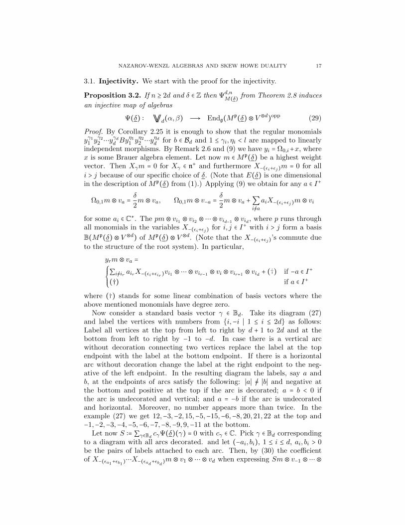
Now consider a standard basis vector γ ∈ Bd. Take its diagram (27)and label the vertices with numbers from i,−i ∣ 1 ≤ i ≤ 2d as follows:Label all vertices at the top from left to right by d + 1 to 2d and at thebottom from left to right by −1 to −d. In case there is a vertical arcwithout decoration connecting two vertices replace the label at the topendpoint with the label at the bottom endpoint. If there is a horizontalarc without decoration change the label at the right endpoint to the neg-ative of the left endpoint. In the resulting diagram the labels, say a andb, at the endpoints of arcs satisfy the following: ∣a∣ /= ∣b∣ and negative atthe bottom and positive at the top if the arc is decorated; a = b < 0 ifthe arc is undecorated and vertical; and a = −b if the arc is undecoratedand horizontal. Moreover, no number appears more than twice. In theexample (27) we get 12,−3,−2,15,−5,−15,−6,−8,20,21,22 at the top and−1,−2,−3,−4,−5,−6,−7,−8,−9,9,−11 at the bottom.
Let now S ∶= ∑γ∈Bd cγΨ(δ)(γ) = 0 with cγ ∈ C. Pick γ ∈ Bd correspondingto a diagram with all arcs decorated. and let (−ai, bi), 1 ≤ i ≤ d, ai, bi > 0be the pairs of labels attached to each arc. Then, by (30) the coefficientof X−(εa1+εb1)
⋯X−(εad+εbd)m ⊗ v1 ⊗⋯⊗ vd when expressing Sm ⊗ v−1 ⊗⋯⊗
18 MICHAEL EHRIG AND CATHARINA STROPPEL
v−d in our basis is precisely cγ , hence cγ = 0. Repeating this argumentgives cγ = 0 for all diagrams with all strands decorated. Next pick b ∈ Bdwhich corresponds to a diagram with all arcs except one decorated and letj1, . . . jd and j′1, . . . j
′d be the associated labels at the bottom respectively
top of the diagram read from left to right. Let (−ai, bi), 1 ≤ i ≤ d − 1,ai, bi > 0 be the pairs of labels attached to each arc. By (30), the coefficientof X−(εa1+εb1)
⋯X−(εad−1+εbd−1)m⊗vi1 ⊗⋯vid when expressing Sm⊗vj1 ⊗⋯vjd
in our basis is then precisely cγ . Hence cγ = 0 for all diagrams with only oneundecorated arc. Proceeding like this gives finally cγ = 0 for all γ. Hencethe linearly independence follows.
3.2. Weight diagrams and bipartitions. Based on [AMR06] we intro-duce a labelling set for a basis in the cyclotomic quotients and connect itwith the counting of Verma modules from Lemma 2.16 via the diagrammaticweights.
Fix integers d and t with 0 ≤ t ≤ ⌊d2⌋. A partition of d is a sequenceλ = (λ1, λ2,⋯) of weakly decreasing non-negative integers λi which sum upto d, i.e. ∣λ∣ ∶= ∑i≥1 λi = d. As usual we identify a partition with its Ferresor Young diagram containing λi boxes in the i-th row. Its top left vertex iscalled the origin. A bipartition is an ordered pair λ = (λ1, λ2) of partitionsλ1, λ2. We denote by P2 (resp. P2(d)) the set of bipartitions (of d) andby P1 (resp. P1(d)) the set of partitions (of d). An up-down-bitableauis a sequence (∅,∅) = λ(0), λ(1),⋯, λ(d) of bipartitions starting from theempty bipartition and such that λ(i + 1) differs from λ(i) by removing oradding exactly one box. If the length of the sequence is d + 1 we call it alsoan up-down-d-bitableau. The set of all up-down-bitableaux is denoted T 2
with the subset T 2d of all up-down-d-bitableaux and the subset T 1
d (λ) of allλ-up-down-tableaux. i.e. all those up-down-d-bitableau ending at a fixedbipartition λ. Similarly we define the sets T 1, T 1
d , T 1d (λ) of all up-down-
tableaux, all up-down-d-tableaux and λ-up-down-d-tableaux for a partitionλ. From [AMR06] it follows in particular that for l = 1,2
∑λ
∣Tld (λ)∣
2= ld(2d − 1)!! (30)
As defined in Section 1 we associate a diagrammatic weight to each weightin Λ. For simplicity we will denote this by the same letter and in light ofCorollary 3.6 stick here to the case δ ≥ 0. Then the corresponding dia-grammatic weights are the following. (The first and third are diagrammatic
NAZAROV-WENZL ALGEBRAS AND SKEW HOWE DUALITY 19
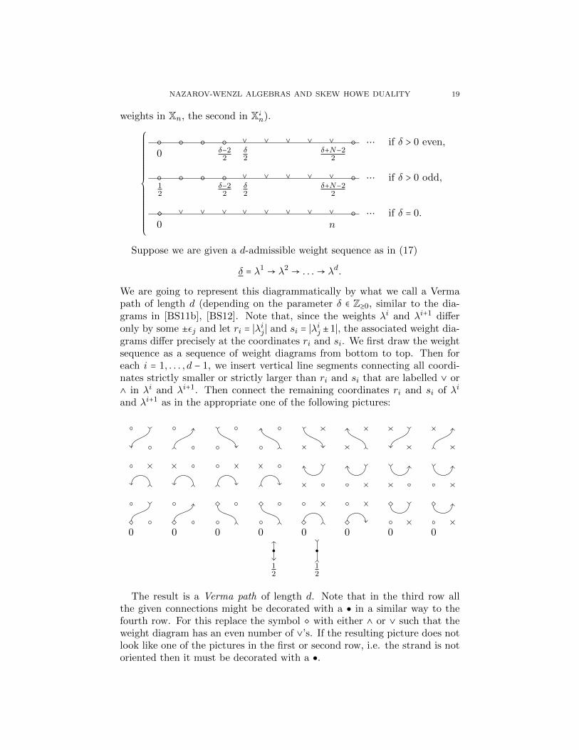
weights in Xn, the second in X n).
⎧⎪⎪⎪⎪⎪⎪⎪⎪⎪⎪⎪⎪⎪⎪⎪⎪⎨⎪⎪⎪⎪⎪⎪⎪⎪⎪⎪⎪⎪⎪⎪⎪⎪⎩
0
δ−22
∨
δ2
∨ ∨ ∨ ∨
δ+N−22
⋯ if δ > 0 even,
12
δ−22
∨
δ2
∨ ∨ ∨ ∨
δ+N−22
⋯ if δ > 0 odd,
0
∨ ∨ ∨ ∨ ∨ ∨ ∨ ∨
n ⋯ if δ = 0.
Suppose we are given a d-admissible weight sequence as in (17)
δ = λ1→ λ2
→ . . .→ λd.
We are going to represent this diagrammatically by what we call a Vermapath of length d (depending on the parameter δ ∈ Z≥0, similar to the dia-grams in [BS11b], [BS12]. Note that, since the weights λi and λi+1 differonly by some ±εj and let ri = ∣λij ∣ and si = ∣λij ±1∣, the associated weight dia-grams differ precisely at the coordinates ri and si. We first draw the weightsequence as a sequence of weight diagrams from bottom to top. Then foreach i = 1, . . . , d − 1, we insert vertical line segments connecting all coordi-nates strictly smaller or strictly larger than ri and si that are labelled ∨ or∧ in λi and λi+1. Then connect the remaining coordinates ri and si of λi
and λi+1 as in the appropriate one of the following pictures:
0 0 0 0 0 0 0 0
12
12
The result is a Verma path of length d. Note that in the third row allthe given connections might be decorated with a in a similar way to thefourth row. For this replace the symbol with either ∧ or ∨ such that theweight diagram has an even number of ∨’s. If the resulting picture does notlook like one of the pictures in the first or second row, i.e. the strand is notoriented then it must be decorated with a .
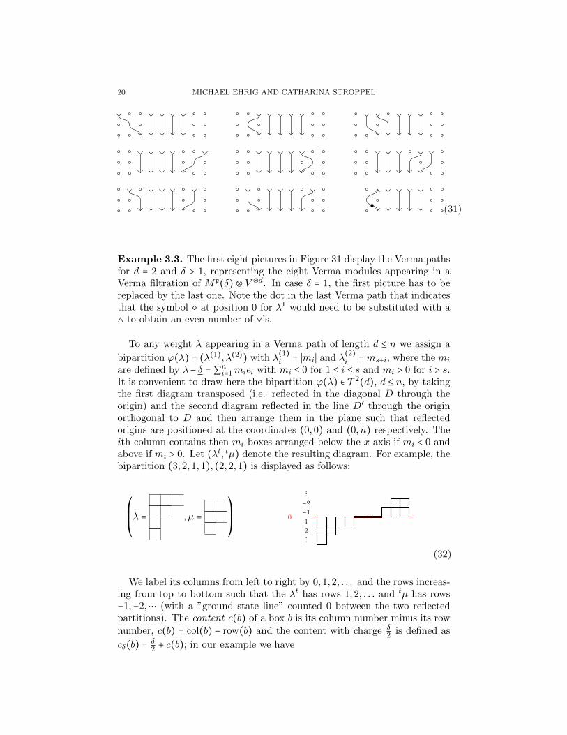
20 MICHAEL EHRIG AND CATHARINA STROPPEL
(31)
Example 3.3. The first eight pictures in Figure 31 display the Verma pathsfor d = 2 and δ > 1, representing the eight Verma modules appearing in aVerma filtration of Mp(δ) ⊗ V ⊗d. In case δ = 1, the first picture has to bereplaced by the last one. Note the dot in the last Verma path that indicatesthat the symbol at position 0 for λ1 would need to be substituted with a∧ to obtain an even number of ∨’s.
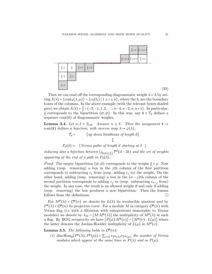
To any weight λ appearing in a Verma path of length d ≤ n we assign a
bipartition ϕ(λ) = (λ(1), λ(2)) with λ(1)i = ∣mi∣ and λ
(2)i =ms+i, where the mi
are defined by λ− δ = ∑ni=1miεi with mi ≤ 0 for 1 ≤ i ≤ s and mi > 0 for i > s.It is convenient to draw here the bipartition ϕ(λ) ∈ T 2(d), d ≤ n, by takingthe first diagram transposed (i.e. reflected in the diagonal D through theorigin) and the second diagram reflected in the line D′ through the originorthogonal to D and then arrange them in the plane such that reflectedorigins are positioned at the coordinates (0,0) and (0, n) respectively. Theith column contains then mi boxes arranged below the x-axis if mi < 0 andabove if mi > 0. Let (λt, tµ) denote the resulting diagram. For example, thebipartition (3,2,1,1), (2,2,1) is displayed as follows:
⎛⎜⎜⎝
λ = , µ =
⎞⎟⎟⎠
⋮
−2
−1
1
2
⋮
0
(32)
We label its columns from left to right by 0,1,2, . . . and the rows increas-ing from top to bottom such that the λt has rows 1,2, . . . and tµ has rows−1,−2,⋯ (with a ”ground state line” counted 0 between the two reflectedpartitions). The content c(b) of a box b is its column number minus its row
number, c(b) = col(b) − row(b) and the content with charge δ2 is defined as
cδ(b) =δ2 + c(b); in our example we have
NAZAROV-WENZL ALGEBRAS AND SKEW HOWE DUALITY 21
δ2 -1
δ2 -2
δ2 -3
δ2
δ2 -1
δ2+1 δ
2+2
δ2+n-2
δ2+n
δ2+n-1
δ2+n+1
δ2+n
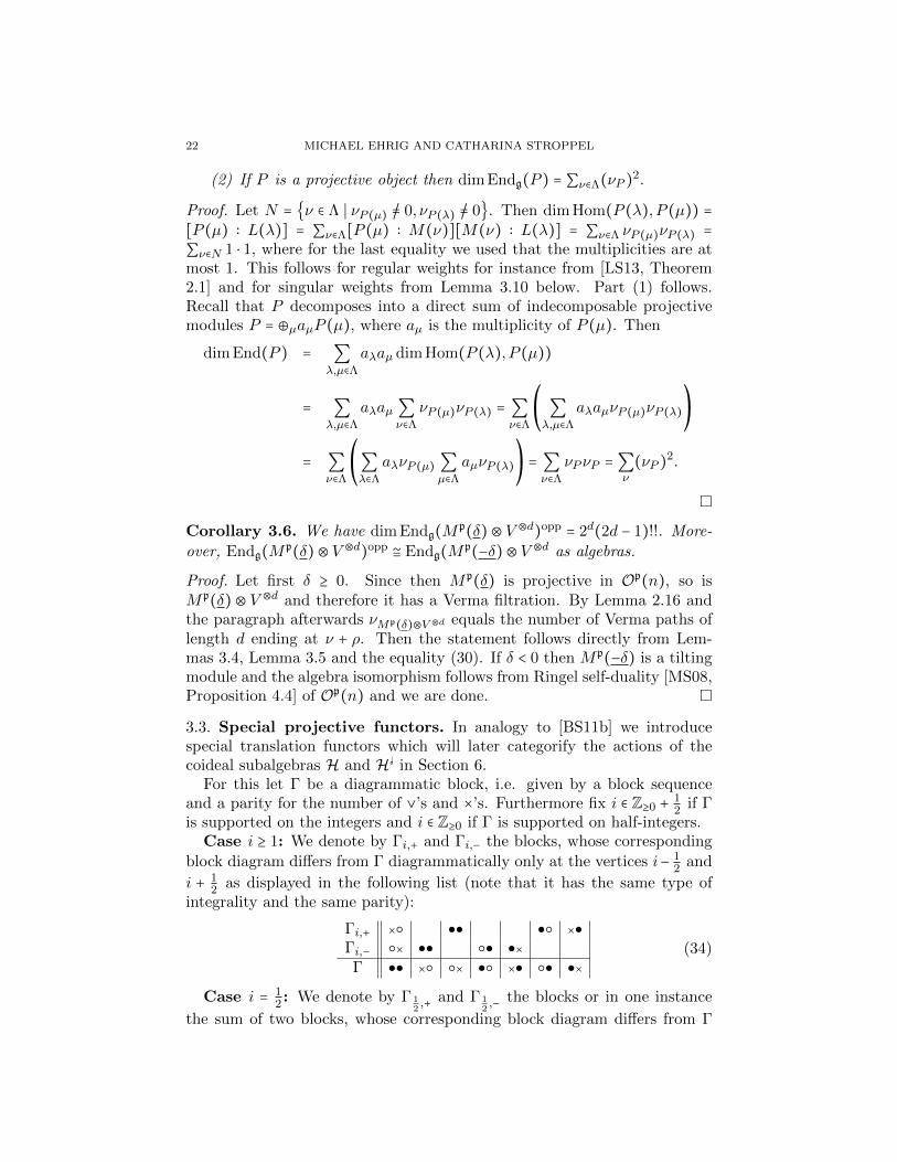
(33)
Then we can read off the corresponding diagrammatic weight λ ∈ Λ by set-ting I(λ) = contδ(λ,µ) = cδ(bi) ∣ 1 ≤ i ≤ n, where the bi are the boundaryboxes of the columns. In the above example (with the relevant boxes shaded
grey) we obtain I(λ) = δ2 +−3,−1,1,2, . . . , n−4, n−2, n, n+1. In particular,
δ corresponds to the bipartition (∅,∅). In this way, any t ∈ Td defines asequence cont(t) of diagrammatic weights.
Lemma 3.4. Let n, δ ∈ Z≥0. Assume n ≥ δ. Then the assignment t ↦cont(t) defines a bijection, with inverse map λ↦ ϕ(λ),
Td = up-down bitableaux of length d
Pd(δ) ∶= Verma paths of length d starting at δ
inducing also a bijection between ⋃0≤k≤⌊ d2⌋P2(d − 2k) and the set of weights
appearing at the end of a path in Pd(δ).
Proof. The empty bipartition (∅,∅) corresponds to the weight δ + ρ. Nowadding (resp. removing) a box in the jth column of the first partitioncorresponds to subtracting εj from (resp. adding εj to) the weight. On theother hand, adding (resp. removing) a box in the (n − j)th column of thesecond partition corresponds to adding εj to (resp. subtracting εn−j from)the weight. In any case, the result is an allowed weight if and only if adding(resp. removing) the box produces a new bipartition. Then the lemmafollows from the definitions.
For Mp(λ) ∈ Op(n) we denote by L(λ) its irreducible quotient and byP p(λ) ∈ Op(n) its projective cover. For a module M in category Op(n) withVerma flag (i.e with a filtration with subquotients isomorphic to Vermamodules) we denote by λM = [M ∶Mp(λ)] the multiplicity of Mp(λ) in sucha flag. By BGG reciprocity we have [P (µ)∶Mp(ν)] = [Mp(ν) ∶ L(µ)] wherethe latter denotes the Jordan-Hoelder multiplicity of L(µ) in Mp(ν).
Lemma 3.5. The following holds in Op(n):
(1) dim Homg(Pp(λ), P p(µ)) = ∑ν∈Λ νP p(λ)νP p(µ), the number of Verma
modules which appear at the same time in P (λ) and in P (µ).
22 MICHAEL EHRIG AND CATHARINA STROPPEL
(2) If P is a projective object then dim Endg(P ) = ∑ν∈Λ(νP )2.
Proof. Let N = ν ∈ Λ ∣ νP (µ) /= 0, νP (λ) /= 0. Then dim Hom(P (λ), P (µ)) =[P (µ) ∶ L(λ)] = ∑ν∈Λ[P (µ) ∶ M(ν)][M(ν) ∶ L(λ)] = ∑ν∈Λ νP (µ)νP (λ) =
∑ν∈N 1 ⋅ 1, where for the last equality we used that the multiplicities are atmost 1. This follows for regular weights for instance from [LS13, Theorem2.1] and for singular weights from Lemma 3.10 below. Part (1) follows.Recall that P decomposes into a direct sum of indecomposable projectivemodules P = ⊕µaµP (µ), where aµ is the multiplicity of P (µ). Then
dim End(P ) = ∑λ,µ∈Λ
aλaµ dim Hom(P (λ), P (µ))
= ∑λ,µ∈Λ
aλaµ∑ν∈Λ
νP (µ)νP (λ) = ∑ν∈Λ
⎛
⎝∑λ,µ∈Λ
aλaµνP (µ)νP (λ)
⎞
⎠
= ∑ν∈Λ
⎛
⎝∑λ∈Λ
aλνP (µ) ∑µ∈Λ
aµνP (λ)
⎞
⎠= ∑ν∈Λ
νP νP =∑ν
(νP )2.
Corollary 3.6. We have dim Endg(Mp(δ)⊗ V ⊗d)opp = 2d(2d − 1)!!. More-
over, Endg(Mp(δ)⊗ V ⊗d)opp ≅ Endg(M
p(−δ)⊗ V ⊗d as algebras.
Proof. Let first δ ≥ 0. Since then Mp(δ) is projective in Op(n), so isMp(δ) ⊗ V ⊗d and therefore it has a Verma filtration. By Lemma 2.16 andthe paragraph afterwards νMp(δ)⊗V ⊗d equals the number of Verma paths oflength d ending at ν + ρ. Then the statement follows directly from Lem-mas 3.4, Lemma 3.5 and the equality (30). If δ < 0 then Mp(−δ) is a tiltingmodule and the algebra isomorphism follows from Ringel self-duality [MS08,Proposition 4.4] of Op(n) and we are done.
3.3. Special projective functors. In analogy to [BS11b] we introducespecial translation functors which will later categorify the actions of thecoideal subalgebras H and H in Section 6.
For this let Γ be a diagrammatic block, i.e. given by a block sequenceand a parity for the number of ∨’s and ×’s. Furthermore fix i ∈ Z≥0 +
12 if Γ
is supported on the integers and i ∈ Z≥0 if Γ is supported on half-integers.Case i ≥ 1: We denote by Γi,+ and Γi,− the blocks, whose corresponding
block diagram differs from Γ diagrammatically only at the vertices i− 12 and
i + 12 as displayed in the following list (note that it has the same type of
integrality and the same parity):
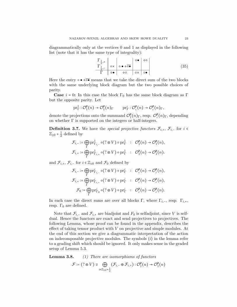
Γi,+ × ×
Γi,− × ×
Γ × × × ×
(34)
Case i = 12 : We denote by Γ 1
2,+ and Γ 1
2,− the blocks or in one instance
the sum of two blocks, whose corresponding block diagram differs from Γ
NAZAROV-WENZL ALGEBRAS AND SKEW HOWE DUALITY 23
diagrammatically only at the vertices 0 and 1 as displayed in the followinglist (note that it has the same type of integrality):
Γ 12,+
Γ 12,− × +
Γ ×
(35)
Here the entry + means that we take the direct sum of the two blockswith the same underlying block diagram but the two possible choices ofparity.
Case i = 0: In this case the block Γ0 has the same block diagram as Γbut the opposite parity. Let
pr1Γ ∶ O
p1(n)→ O
p1(n)Γ pr
Γ ∶ Op (n)→ O
p (n)Γ,
denote the projections onto the summand Op1(n)Γ, resp. Op
(n)Γ, dependingon whether Γ is supported on the integers or half-integers.
Definition 3.7. We have the special projective functors Fi,+, Fi,− for i ∈
Z≥0 +12 defined by
Fi,− ∶=⊕Γ
pr1Γi,− (?⊗ V ) pr1
Γ ∶ Op1(n)→ O
p1(n),
Fi,+ ∶=⊕Γ
pr1Γi,+ (?⊗ V ) pr1
Γ ∶ Op1(n)→ O
p1(n).
and Fi,+, Fi,− for i ∈ Z≥0 and F0 defined by
Fi,− ∶=⊕Γ
pr Γi,− (?⊗ V ) pr
Γ ∶ Op (n)→ O
p (n),
Fi,+ ∶=⊕Γ
pr Γi,+ (?⊗ V ) pr
Γ ∶ Op (n)→ O
p (n),
F0 ∶=⊕Γ
pr Γ0(?⊗ V ) pr
Γ ∶ Op (n)→ O
p (n).
In each case the direct sums are over all blocks Γ, where Γi,−, resp. Γi,+,resp. Γ0 are defined.
Note that Fi,− and Fi,+ are biadjoint and F0 is selfadjoint, since V is self-dual. Hence the functors are exact and send projectives to projectives. Thefollowing Lemma, whose proof can be found in the appendix, describes theeffect of taking tensor product with V on projective and simple modules. Atthe end of this section we give a diagrammatic interpretation of the actionon indecomposable projective modules. The symbols ⟨i⟩ in the lemma referto a grading shift which should be ignored. It only makes sense in the gradedsetup of Lemma 5.3.
Lemma 3.8. (1) There are isomorphisms of functors
F ∶= (?⊗ V ) ≅ ⊕i∈Z≥0+ 1
2
(Fi,− ⊕Fi,+) ∶ Op1(n)→ O
p1(n)
24 MICHAEL EHRIG AND CATHARINA STROPPEL
and
F ∶= (?⊗ V ) ≅ ⊕
i∈Z>0(Fi,− ⊕Fi,+)⊕F0 ∶ O
p (n)→ O
p (n).
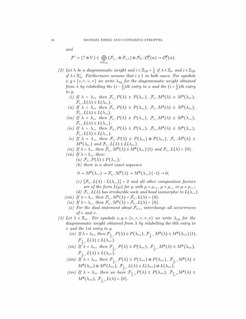
(2) Let λ be a diagrammatic weight and i ∈ Z≥0 +12 if λ ∈ Xn and i ∈ Z≥0
if λ ∈ X n. Furthermore assume that i ≥ 1 in both cases. For symbols
x, y ∈ ,∧,∨,× we write λxy for the diagrammatic weight obtained
from λ by relabelling the (i − 12)th entry to x and the (i + 1
2)th entryto y.
(i) If λ = λ∨ then Fi,−P (λ) ≅ P (λ∨), Fi,−Mp(λ) ≅ Mp(λ∨),
Fi,−L(λ) ≅ L(λ∨).(ii) If λ = λ∧ then Fi,−P (λ) ≅ P (λ∧), Fi,−M
p(λ) ≅ Mp(λ∧),Fi,−L(λ) ≅ L(λ∧).
(iii) If λ = λ×∨ then Fi,−P (λ) ≅ P (λ∨×), Fi,−Mp(λ) ≅ Mp(λ∨×),
Fi,−L(λ) ≅ L(λ∨×).(iv) If λ = λ×∧ then Fi,−P (λ) ≅ P (λ∧×), Fi,−M
p(λ) ≅ Mp(λ∧×),Fi,−L(λ) ≅ L(λ∧×).
(v) If λ = λ∨∧ then Fi,−P (λ) ≅ P (λ×) ⊕ P (λ×), Fi,−Mp(λ) ≅
Mp(λ×) and Fi,−L(λ) ≅ L(λ×).(vi) If λ = λ∧∨ then Fi,−M
p(λ) ≅Mp(λ×) ⟨1⟩ and Fi,−L(λ) = 0.(vii) If λ = λ× then:
(a) Fi,−P (λ) ≅ P (λ∨∧);(b) there is a short exact sequence
0→Mp(λ∧∨)→ Fi,−M
p(λ)→Mp
(λ∨∧) ⟨−1⟩→ 0;
(c) [Fi,−L(λ) ∶ L(λ∨∧)] = 2 and all other composition factorsare of the form L(µ) for µ with µ = µ∨∨, µ = µ∧∧ or µ = µ∧∨;
(d) Fi,−L(λ) has irreducible socle and head isomorphic to L(λ∨∧).(viii) If λ = λ∨∨ then Fi,−M
p(λ) = Fi,−L(λ) = 0.(ix) If λ = λ∧∧ then Fi,−M
p(λ) = Fi,−L(λ) = 0.(x) For the dual statement about Fi,+, interchange all occurrences
of and ×.(3) Let λ ∈ Xn. For symbols x, y ∈ ,∧,∨,×, we write λxy for the
diagrammatic weight obtained from λ by relabelling the 0th entry tox and the 1st entry to y
(xi) If λ = λ∨ then F 12,−P (λ) ≅ P (λ×), F 1
2,−M
p(λ) ≅Mp(λ×) ⟨1⟩,
F 12,−L(λ) ≅ L(λ×).
(xii) If λ = λ∧ then F 12,−P (λ) ≅ P (λ×), F 1
2,−M
p(λ) ≅ Mp(λ×),
F 12,−L(λ) ≅ L(λ×).
(xiii) If λ = λ then F 12,−P (λ) ≅ P (λ∧) ⊕ P (λ∨), F 1
2,−M
p(λ) ≅
Mp(λ∧)⊕Mp(λ∨), F 1
2,−L(λ) ≅ L(λ∧)⊕L(λ∨).
(xiv) If λ = λ∨ then we have F 12,+P (λ) ≅ P (λ), F 1
2,+M
p(λ) ≅
Mp(λ), F 12,+L(λ) = 0.
NAZAROV-WENZL ALGEBRAS AND SKEW HOWE DUALITY 25
(xv) If λ = λ∧ then F 12,+P (λ) ≅ P (λ), F 1
2,+M
p(λ) ≅ Mp(λ),
F 12,+L(λ) = 0.
(xvi) If λ = λ× then:(a) F 1
2,+P (λ) ≅ P (λ∧);
(b) there is a short exact sequence
0→Mp(λ∨)→ F 1
2,+M
p(λ)→Mp
(λ∧) ⟨−1⟩→ 0;
(c) [F 12,+L(λ)∶L(∧)] = 2 and all other composition factors
are of the form L(µ) for µ with µ = µ∨,(xvii) If λ = λ× then we have F 1
2,−P (λ) = 0, F 1
2,−M
p(λ) = 0,
F 12,−L(λ) = 0.
(xviii) If λ = λ then we have F 12,−P (λ) = 0, F 1
2,−M
p(λ) = 0,
F 12,−L(λ) = 0.
(4) Finally assume λ ∈ X n. For symbols x ∈ ,∧,∨,× we write λx for
the diagrammatic weight obtained from λ by relabelling the 12 th entry
to x. Then we have(xiv) If λ = λ∧ then F0P (λ) ≅ P (λ∨), F0M
p(λ) ≅Mp(λ∨), F0L(λ) ≅L(λ∨).
(xiv) If λ = λ∨ then F0P (λ) ≅ P (λ∧), F0Mp(λ) ≅Mp(λ∧), F0L(λ) ≅
L(λ∧).
Remark 3.9. Note that each of the Fi,+, Fi,−, F0 is a translation functor inthe sense of [Hum08]. It is either an equivalence of categories, a translationfunctor to the wall, a translation functor out of the wall or, in the specialcase of F 1
2,− and the choice of a specific block diagram a direct sum of two
translation functors out of the wall. In contrast to the type A situation from[BS11b] not all translations to walls appear however as summands.
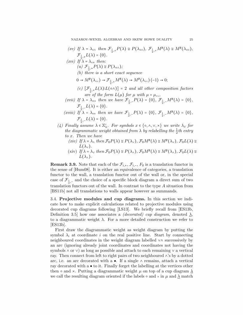
3.4. Projective modules and cup diagrams. In this section we indi-cate how to make explicit calculations related to projective modules usingdecorated cup diagrams following [LS13]. We briefly recall from [ES13b,Definition 3.5] how one associates a (decorated) cup diagram, denoted λ,to a diagrammatic weight λ. For a more detailed construction we refer to[ES13b].
First draw the diagrammatic weight as weight diagram by putting thesymbol λi at coordinate i on the real positive line. Start by connectingneighboured coordinates in the weight diagram labelled ∨∧ successively byan arc (ignoring already joint coordinates and coordinates not having thesymbols ∧ or ∨) as long as possible and attach to each remaining ∨ a verticalray. Then connect from left to right pairs of two neighboured ∧’s by a dottedarc, i.e. an arc decorated with a . If a single ∧ remains, attach a verticalray decorated with a to it. Finally forget the labelling at the vertices otherthen and ×. Putting a diagrammatic weight µ on top of a cup diagram λwe call the resulting diagram oriented if the labels and × in µ and λ match
26 MICHAEL EHRIG AND CATHARINA STROPPEL
precisely, undecorated rays are labelled ∨ and decorated rays are labelled∧ and every undecorated cup has exactly one ∧ and one ∨ whereas anydecorated cup has either two ∨’s or two ∧’s at its endpoints.
The multiplicities µP (λ) are then easily calculated:
Lemma 3.10.
µP (λ) =
⎧⎪⎪⎨⎪⎪⎩
1 if µλ is oriented
0 if µλ is not oriented.
Proof. For regular weights, i.e. weights which do not contain ×’s or ’s thiswas proved is [LS13, Theorem 2.1]. (Lemma 4.3 therein and the paragraphafterwards makes the translation into our setup.) For singular weights ob-serve that diagrammatically the numbers stay the same if we remove the ×’sand ’s. This corresponds Lie theoretically to the Enright-Shelton equiva-lence [ES87] between singular blocks and regular blocks for smaller rank Liealgebras, and hence the multiplicities agree.
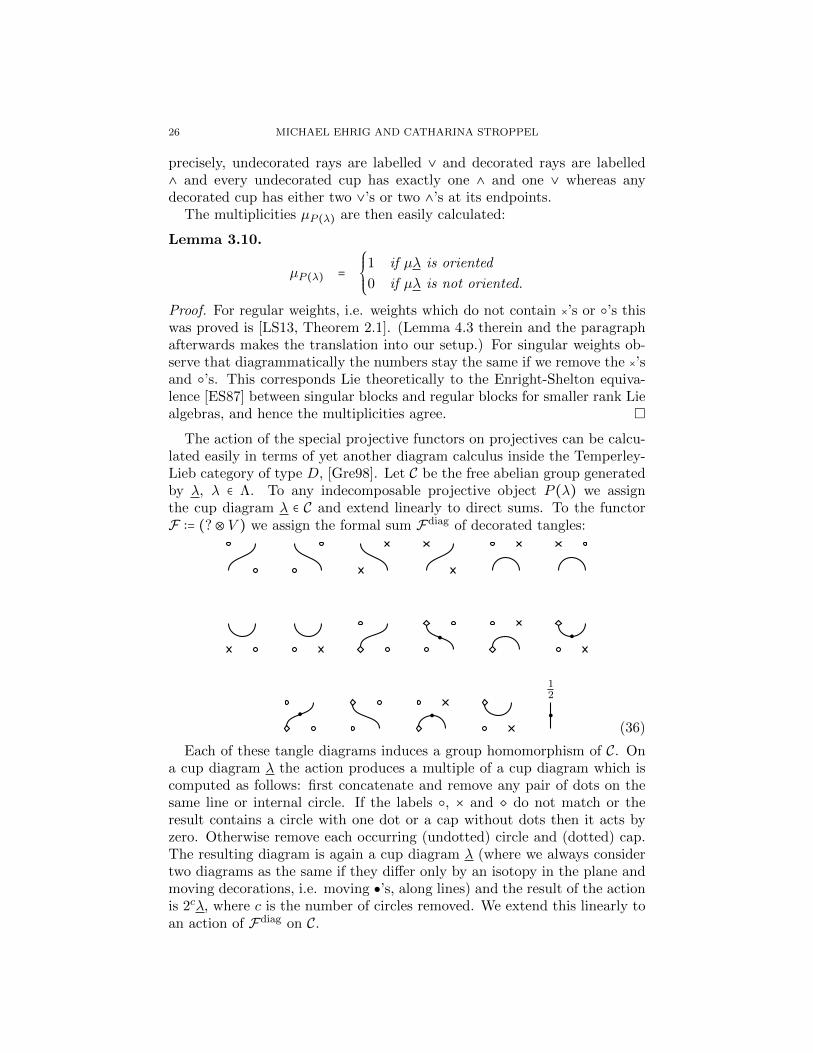
The action of the special projective functors on projectives can be calcu-lated easily in terms of yet another diagram calculus inside the Temperley-Lieb category of type D, [Gre98]. Let C be the free abelian group generatedby λ, λ ∈ Λ. To any indecomposable projective object P (λ) we assignthe cup diagram λ ∈ C and extend linearly to direct sums. To the functorF ∶= (?⊗ V ) we assign the formal sum Fdiag of decorated tangles:
12
(36)
Each of these tangle diagrams induces a group homomorphism of C. Ona cup diagram λ the action produces a multiple of a cup diagram which iscomputed as follows: first concatenate and remove any pair of dots on thesame line or internal circle. If the labels , × and do not match or theresult contains a circle with one dot or a cap without dots then it acts byzero. Otherwise remove each occurring (undotted) circle and (dotted) cap.The resulting diagram is again a cup diagram λ (where we always considertwo diagrams as the same if they differ only by an isotopy in the plane andmoving decorations, i.e. moving ’s, along lines) and the result of the actionis 2cλ, where c is the number of circles removed. We extend this linearly toan action of Fdiag on C.
NAZAROV-WENZL ALGEBRAS AND SKEW HOWE DUALITY 27
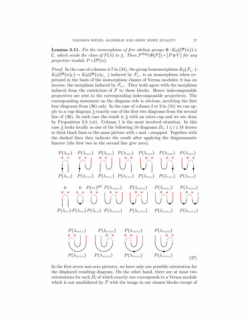
Lemma 3.11. Fix the isomorphism of free abelian groups Φ ∶K0(Op(n)) ≅
C, which sends the class of P (λ) to λ. Then Fdiag(Φ[P ]) = [P ⊗V ] for anyprojective module P ∈ Op(n).
Proof. In the case of columns 4-7 in (34), the group homomorphismK0(Fi,−) ∶
K0(Op(n)Γ) → K0(O
p(n)Γi,−) induced by Fi,− is an isomorphism when ex-pressed in the basis of the isomorphism classes of Verma modules; it has aninverse, the morphism induced by Fi,+. They both agree with the morphisminduced from the restriction of F to these blocks. Hence indecomposableprojectives are sent to the corresponding indecomposable projectives. Thecorresponding statement on the diagram side is obvious, involving the firstfour diagrams from (36) only. In the case of column 2 or 3 in (34) we can ap-ply to a cup diagram λ exactly one of the first two diagrams from the secondline of (36). In each case the result is λ with an extra cup and we are doneby Proposition 3.8 (vii). Column 1 is the most involved situation. In thiscase λ looks locally as one of the following 18 diagrams Di, 1 ≤ i ≤ 18 drawnin thick black lines or the same picture with and × swapped. Together withthe dashed lines they indicate the result after applying the diagrammaticfunctor (the first two in the second line give zero).
P (λ∧∨)
P (λ×)
P (λ∧∨∧)
P (λ×∧)
P (λ∨∨∧)
P (λ×∧)
P (λ∨∧∨)
P (λ∨×)
P (λ∧∧∨)
P (λ∧×)
P (λ∨∧∧)
P (λ∨×)
P (λ∧∧∧)
P (λ∨×)
P (λ∨∨)
0
P (λ∧∧)
0
P (λ∨∧)
P (×)⊕2
P (λ∨∧∨∧)
P (λ∨×∧)
P (λ∧∧∨∧)
P (λ∧×∧)
P (λ∨∧∧∧)
P (λ∧×∧)
P (λ∧∧∧∧)
P (λ∨×∧)
P (λ∨∨∧∧)
P (λ×∧∧)
P (λ∨∨∧∧)
P (λ∨∨×)
P (λ∧∨∧∧)
P (λ×∧∧)
P (λ∧∨∧∧)
P (λ∧∨×)
(37)
In the first seven non-zero pictures, we have only one possible orientation forthe displayed resulting diagram. On the other hand, there are at most twoorientations for each Di of which exactly one corresponds to a Verma modulewhich is not annihilated by F with the image in our chosen blocks except of
28 MICHAEL EHRIG AND CATHARINA STROPPEL
the last and penultimate diagram where none of the two is annihilated. Sim-ilar arguments can be used for the functors F 1
2,+, F 1
2,−, and F0. Comparing
with Proposition 3.8 using Lemma 3.10, we see that Fdiag(Φ[P ]) = [P ⊗V ]
in the basis of Verma modules.
As a special case we obtain the following:
Corollary 3.12. Assume we are in case (vi) of Proposition 3.8 and assumethere is no ∨ to the left of our fixed ∧∨ pair then Fi,−P
p(λ) ≅ P p(λ×).
Proof. By assumption and construction, the cup diagram λ looks locally atour two fixed vertices as displayed in one of the pictures in the top line of thefollowing diagram. Applying Fdiag gives for each diagram precisely one newdiagram in the required block as displayed. Hence the statement follows byapplying ϕ−1 and the definition of Fi,−.
4. Cyclotomic quotients
For this whole section we will always assume n ≥ 2d. This isimportant for all statements that involve the idempotent zd introduced inDefinition 4.3.
The action of the commuting y’s decomposes Mp(δ)⊗V ⊗d and ⩔d(α,β)into generalized eigenspaces. Fix the sets J = δ
2 +Z and J< =δ2 +Z<(n−1).
Definition 4.1. We identify ⩔d(α,β) with Endg(Mp(δ)⊗ V ⊗d) via Theo-
rem 3.1. Define the orthogonal weight idempotents e(i), i ∈ Jd characterizedby the property that
e(i)(yr − ir)m= (yr − ir)
m e(i) = 0
for each 1 ≤ r ≤ d and m≫ 0 (for instance m ≥ d is enough).
Then we have the generalized eigenspace decompositions
Mp(δ)⊗ V ⊗d = ∑i∈JdMp(δ)⊗ V ⊗d e(i),
⩔d(α,β) = ∑i∈Jd⩔d(α,β) e(i) and ⩔d(α,β) = ∑i∈Jd e(i)⩔d(α,β)
as right respectively left modules. The quasi-idempotents ek only acts be-tween certain generalized eigenspaces:
Lemma 4.2. Let 1 ≤ k ≤ d − 1. If p ∶= ∑i∈Jd,ik+1=−ik e(i) then we haveek = pek = ekp = pekp. In particular e(i)ek = 0 = ek e(i) if ik+1 /= ik.
Proof. Let m ∈ ⩔d(α,β) or Mp(δ) ⊗ V ⊗d be contained in the generalizedeigenspace for ı, hence m e(i) /= 0. We claim that if mek /= 0 then ir+1+ir = 0.First note that for (yk+yk+1−ik+1−ik)
rm = ∑ra=0(yk−ik)
a(yk+1−ik+1)r−am = 0
for r ≫ 0. Hence m is in the µ ∶= ik+1 + ik-generalized eigenspace for yk+1+yk.Then 0 =m(yk+yk+1−µ)
rek =mek(−µ)k by (8a). Hence µ = 0 and the claim
follows. Since the modules have a generalized eigenspace decompositionpek = 0 = ekp. The rest follows analogously.
NAZAROV-WENZL ALGEBRAS AND SKEW HOWE DUALITY 29
4.1. Semisimplicity.
Definition 4.3. The Brauer algebra idempotent is defined as
zd = ∑i∈(J<)d
e(i). (38)
Multiplication by e(i) projects any ⩔d(α,β)-module onto its i-weightspace, that is, the simultaneous generalised eigenspace for the commutingoperators y1, . . . , yr with respective eigenvalues i1, . . . , ir. By (33), Lemma3.4 and our assumption on n being large, the element zd is just the projectiononto the blocks containing Verma modules indexed by bipartitions of theform (λ,∅) where λ is an up-down-tableau. (The corresponding weights are
precisely those λ which satisfy I(λ) ⊂ [−( δ2 + n − 1), δ2 + n − 1].)
Proposition 4.4. The algebra zd⩔d(α,β)zd has dimension (2d − 1)!!.
Proof. Using Lemma 3.4 and the fact that the algebra has a basis given byVerma paths that correspond to bipartitions of the form (λ,∅) gives theresult.
Theorem 4.5.
(1) The algebra ⩔d(α,β) is semisimple if and only if δ ≥ d − 1.(2) The algebra zd⩔d(α,β)zd is semisimple if and only if δ /= 0 and
δ ≥ d − 1 or δ = 0 and d = 1,3,5.
Proof. Note that Endg(Mp(δ)⊗V ⊗d) is semisimple if and only ifMp(δ)⊗V ⊗d
is a direct sum of projective Verma modules. Or equivalently if all occurringVerma modules have highest weight λ such that λ + ρ is dominant. This isequivalent to the statement that the corresponding diagrammatic weightsdo not contain two ∧’s any pair ∨, ∧ (in this order) or a pair ∧. Startingfrom the diagrammatic weight δ we need precisely δ steps to create an ∧ leftto a ∨, hence δ+2 steps to create a ∨, ∧; we also need 2( δ2 +1) steps to createa pair of two ∧’s and δ + 2 steps to create , ∧. Hence both algebras aresemisimple at least if d < δ+2. Now in case (1), we always can add εn withoutchanging those pairs, an hence the algebra is not semisimple for all d ≥ δ+2.In case (2) with δ /= 0,1 we can always find some at some position < nand hence add or subtract some appropriate εj without changing the pair.That means the truncated algebra is not semisimple for d ≥ δ + 2. For δ = 1we need 3 steps to create a weight starting with ∧ ∨. Hence the algebrais not semisimple and stays not semisimple, since we can always repeatedlyswap the with the ∨ without changing the ∧ pair. Hence (2) holds forany δ > 0. In case δ = 0 one can calculate directly that it is semisimple in thecases d = 1, d = 3, d = 5, but not in the cases d = 2,4,6 and for = 7 we obtaina weight starting with ∧∧∨. Since we can change the last two symbols ∧∨into × and back again without loosing the ∧-pair, the algebra stays notsemisimple for d ≥ 7 and δ = 0. The theorem follows.
30 MICHAEL EHRIG AND CATHARINA STROPPEL
4.2. The basic algebra underlying Endg(Mp(δ)⊗ V ⊗d). Our next goal
is to determine for δ ≥ the projective modules appearing in Mp(δ) ⊗ V ⊗d
and hence the basic algebra underlying Endg(Mp(δ)⊗ V ⊗d) for δ ∈ Z. Our
main tool here is the notion of htδ which measures the minimal length of aVerma path needed to create a Verma module of a given weight.
Definition 4.6. Let δ, d ∈ Z, δ ≥ 0, d ≥ 1 and µ ∈ Λ. The δ-height of µ, htδis defined as htδ(µ) = ∑
ni=1 ∣(δ + ρ)i − (µ + ρ)i∣ = ∑
ni=1 ∣δi − µi∣.
Note that, by Lemma 2.16, the highest weights λ occurring in a Vermafiltration of Mp(δ) ⊗ V ⊗d satisfy htδ(λ) ≤ d and htδ(λ) is precisely thenumber of boxes in ϕ(λ), see (32), (33).
Proposition 4.7. Let δ, d ∈ Z, δ ≥ 0, d ≥ 1. Then Mp(δ)⊗V ⊗d ≅ ⊕µ∈ΛaµP (µ)with multiplicities aµ and aµ /= 0 if and only if htδ ≤ d and d − htδ is even.
Proof. Starting with d = 0 there is only one weight with δ-height zero, namelyδ and the statement is clear. For d = 1 there are two weights, δ−ε1 and δ+εn.Again the statement is clear, since the corresponding two Verma modulesare projective. Now we want to prove the lemma for arbitrary d assumingit for all smaller ones. Note that aµ /= 0 implies that Mp(µ) appears in a
Verma flag of Mp(δ) ⊗ V ⊗d, and hence htδ(µ) ≤ d. Moreover, the highestweights of the occurring Verma modules change in each step by ±εj whichchanges the δ-height either by 1 or −1. By induction, d − htδ(µ) is even.
Conversely, assume µ is a weight with htδ(µ) = d − 2k for some k ≥ 0. If
k > 0 then by induction hypothesis P (µ) appears in M(δ) ⊗ V ⊗d−2. Theweight µ contains at least one neighboured ∧, ∨, or × pair (since onlyfinitely many vertices are labelled ∧, ∨ or ×). Hence we are in one of the cases(i), (ii) or (vii) of Proposition 3.8 so P (µ) is a summand of Fi,+Fi,−P (µ)
and therefore also a summand in Mp(δ)⊗V ⊗d. Now we have to proceed viaa case-by case argument for k = 0:
(1) Assume first that there exist i ∈ I(µ), −i /∈ I(µ) with i ∶= (µ+ρ)a > 0and δa − µa > 0 for some a. (In the diagram picture this means thatthe ath ∨ in δ was moved to the left and gives a ∨ in µ at position i).We assume that a was chosen to be maximal amongst these (thatis the rightmost ∨ which got moved to the left to create some ∨).Locally at the positions i and i + 1 the diagram for µ could look asfollows(a) ∨. In this case set ν = ∨(b) ∨∧. In this case set ν = ×(c) ∨×. In this case set ν = ×∨
(d) ∨∨. Since a was maximal, this means that the ∨ at position i+1forces i + 1 = (µ + ρ)a+1 and at the same time δa+1 − µa+1 ≤ 0which is a contradiction.
In each of the first three cases P (µ) appears as a summand inP (ν)⊗V (by Lemma 3.8 (iii), (vii), (x)) and htδ(ν) = htδ(µ)−1. By
NAZAROV-WENZL ALGEBRAS AND SKEW HOWE DUALITY 31
induction hypothesis P (ν) appears as summand in M(δ) ⊗ V ⊗d−1
and we are done.(2) Assume, (1) does not hold and moreover that if i ∶= (µ + ρ)a > 0
for some a and −i ∉ I then δa − µa = 0. (Diagrammatically thismeans that ∨′s did either not move or turned into ∧′s, creatingpossibly some ×’s). Choose, if it exists, −j ∈ I maximal such that−j < 0. (Diagrammatically we look at the ∧’s and ×’s and choose theleftmost. It sits at position j). Locally at the positions j − 1 and j,for j > 1
2 , the diagram for µ could look as follows(a) ∧. In this case set ν = ×.(b) ∨∧. In this case set ν = ×.(c) ∧. In this case set ν = ∧.(d) ∨×. In this case set ν = ×∨.(e) ×. In this case set ν = ∧∨. The ∨ in δ at place j − 1 got
moved, hence turned into an ∧ or created a ×. But then thesame happened to all the ∨’s further to the left. In particular,ν has no ∨ left of the ∧ at position j and hence we can applyLemma 3.12 to P (ν).
Again, in each of the last four cases P (µ) appears as a summandin P (ν) ⊗ V by Proposition 3.8 and by induction hypothesis P (ν)appears as summand in M(δ) ⊗ V ⊗d−1. In case no ∧ or × exists weeither have µ = δ and there is nothing to do or µ has a ∨ or ∨ pairwhich we swap to create a new weight ν and argue as above usingProposition 3.8 (i) or (iii) with (x).
(3) Assume finally that neither (1) nor (2) holds. The arguments arecompletely analogous to (2) except for the case(e’) ×. In case there is no ∨ to the left of the cross we set ν = ∧∨
and argue as before using Lemma 3.12. Otherwise such a ∨ didnot get moved or got moved to the right, since we excluded case(1). Since it is separated from our × at position j by a , our × iscreated from a ∨ which got moved to the right. Hence changing× to ∨∧ decreases the height by 1. Then we can argue againusing Proposition 3.8, this time part (v).
Lemma 4.8. Let δ, d ∈ Z, δ ≥ 0, d ≥ 1. The set
S = S(δ, d) = µ ∈ Λ ∣ htδ(µ) ≤ d,htδ(µ) ≡ d mod 2 (39)
is saturated in the following sense: if µ ∈ S and ν ∈ Λ such that µ and ν arein the same block and ν ≥ λ then ν ∈ S.
Proof. Assume µ is in the same block as ν, µ < ν. Then the diagrammaticweight for ν is obtained from µ by applying a finite sequence of changesfrom ∧∧ to ∨∨ or from ∨∧ to ∧∨ at positions only separated by ′ and ×’s.Hence it is enough to consider these basic changes.
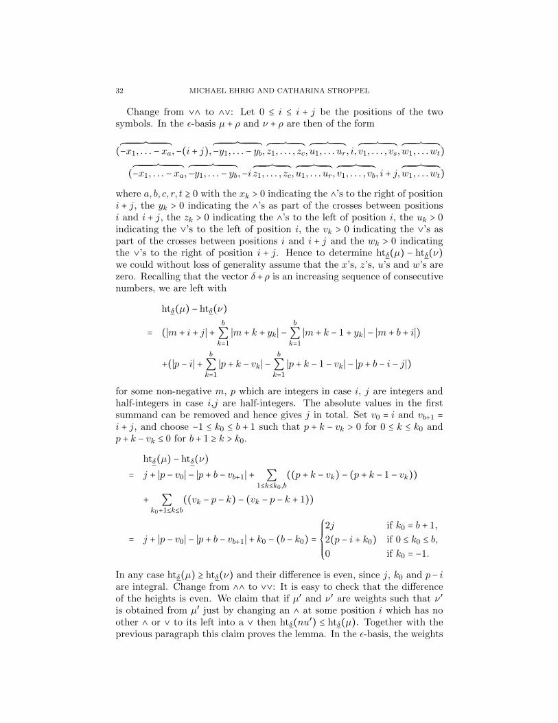
32 MICHAEL EHRIG AND CATHARINA STROPPEL
Change from ∨∧ to ∧∨: Let 0 ≤ i ≤ i + j be the positions of the twosymbols. In the ε-basis µ + ρ and ν + ρ are then of the form
(³¹¹¹¹¹¹¹¹¹¹¹¹¹¹¹¹¹¹¹¹¹¹¹¹¹¹¹·¹¹¹¹¹¹¹¹¹¹¹¹¹¹¹¹¹¹¹¹¹¹¹¹¹¹¹¹µ−x1, . . . − xa,−(i + j),
³¹¹¹¹¹¹¹¹¹¹¹¹¹¹¹¹¹¹¹¹¹¹¹¹¹·¹¹¹¹¹¹¹¹¹¹¹¹¹¹¹¹¹¹¹¹¹¹¹¹¹¹µ−y1, . . . − yb,
³¹¹¹¹¹¹¹¹¹¹¹¹¹¹¹·¹¹¹¹¹¹¹¹¹¹¹¹¹¹¹¹µz1, . . . , zc,
³¹¹¹¹¹¹¹¹¹¹¹¹¹¹·¹¹¹¹¹¹¹¹¹¹¹¹¹¹µu1, . . . ur, i,
³¹¹¹¹¹¹¹¹¹¹¹¹¹¹¹¹·¹¹¹¹¹¹¹¹¹¹¹¹¹¹¹¹µv1, . . . , vs,
³¹¹¹¹¹¹¹¹¹¹¹¹¹¹¹¹·¹¹¹¹¹¹¹¹¹¹¹¹¹¹¹¹µw1, . . .wt)
(³¹¹¹¹¹¹¹¹¹¹¹¹¹¹¹¹¹¹¹¹¹¹¹¹¹¹¹·¹¹¹¹¹¹¹¹¹¹¹¹¹¹¹¹¹¹¹¹¹¹¹¹¹¹¹¹µ−x1, . . . − xa,
³¹¹¹¹¹¹¹¹¹¹¹¹¹¹¹¹¹¹¹¹¹¹¹¹¹·¹¹¹¹¹¹¹¹¹¹¹¹¹¹¹¹¹¹¹¹¹¹¹¹¹¹µ−y1, . . . − yb,−i
³¹¹¹¹¹¹¹¹¹¹¹¹¹¹¹·¹¹¹¹¹¹¹¹¹¹¹¹¹¹¹¹µz1, . . . , zc,
³¹¹¹¹¹¹¹¹¹¹¹¹¹¹·¹¹¹¹¹¹¹¹¹¹¹¹¹¹µu1, . . . ur,
³¹¹¹¹¹¹¹¹¹¹¹¹¹¹¹¹·¹¹¹¹¹¹¹¹¹¹¹¹¹¹¹¹µv1, . . . , vb, i + j,
³¹¹¹¹¹¹¹¹¹¹¹¹¹¹¹¹·¹¹¹¹¹¹¹¹¹¹¹¹¹¹¹¹µw1, . . .wt)
where a, b, c, r, t ≥ 0 with the xk > 0 indicating the ∧’s to the right of positioni + j, the yk > 0 indicating the ∧’s as part of the crosses between positionsi and i + j, the zk > 0 indicating the ∧’s to the left of position i, the uk > 0indicating the ∨’s to the left of position i, the vk > 0 indicating the ∨’s aspart of the crosses between positions i and i + j and the wk > 0 indicatingthe ∨’s to the right of position i + j. Hence to determine htδ(µ) − htδ(ν)we could without loss of generality assume that the x’s, z’s, u’s and w’s arezero. Recalling that the vector δ+ρ is an increasing sequence of consecutivenumbers, we are left with
htδ(µ) − htδ(ν)
= (∣m + i + j∣ +b
∑k=1
∣m + k + yk∣ −b
∑k=1
∣m + k − 1 + yk∣ − ∣m + b + i∣)
+(∣p − i∣ +b
∑k=1
∣p + k − vk∣ −b
∑k=1
∣p + k − 1 − vk∣ − ∣p + b − i − j∣)
for some non-negative m, p which are integers in case i, j are integers andhalf-integers in case i,j are half-integers. The absolute values in the firstsummand can be removed and hence gives j in total. Set v0 = i and vb+1 =
i + j, and choose −1 ≤ k0 ≤ b + 1 such that p + k − vk > 0 for 0 ≤ k ≤ k0 andp + k − vk ≤ 0 for b + 1 ≥ k > k0.
htδ(µ) − htδ(ν)
= j + ∣p − v0∣ − ∣p + b − vb+1∣ + ∑1≤k≤k0,b
((p + k − vk) − (p + k − 1 − vk))
+ ∑k0+1≤k≤b
((vk − p − k) − (vk − p − k + 1))
= j + ∣p − v0∣ − ∣p + b − vb+1∣ + k0 − (b − k0) =
⎧⎪⎪⎪⎪⎨⎪⎪⎪⎪⎩
2j if k0 = b + 1,
2(p − i + k0) if 0 ≤ k0 ≤ b,
0 if k0 = −1.
In any case htδ(µ) ≥ htδ(ν) and their difference is even, since j, k0 and p− iare integral. Change from ∧∧ to ∨∨: It is easy to check that the differenceof the heights is even. We claim that if µ′ and ν′ are weights such that ν′
is obtained from µ′ just by changing an ∧ at some position i which has noother ∧ or ∨ to its left into a ∨ then htδ(nu
′) ≤ htδ(µ). Together with theprevious paragraph this claim proves the lemma. In the ε-basis, the weights
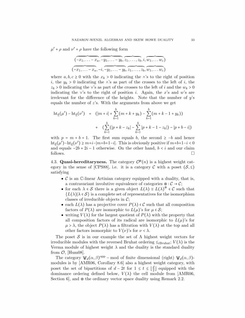
NAZAROV-WENZL ALGEBRAS AND SKEW HOWE DUALITY 33
µ′ + ρ and ν′ + ρ have the following form
(³¹¹¹¹¹¹¹¹¹¹¹¹¹¹¹¹¹¹¹¹¹¹¹¹¹¹¹·¹¹¹¹¹¹¹¹¹¹¹¹¹¹¹¹¹¹¹¹¹¹¹¹¹¹¹¹µ−x1, . . . − xa,
³¹¹¹¹¹¹¹¹¹¹¹¹¹¹¹¹¹¹¹¹¹¹¹¹¹·¹¹¹¹¹¹¹¹¹¹¹¹¹¹¹¹¹¹¹¹¹¹¹¹¹¹µ−y1, . . . − yb,
³¹¹¹¹¹¹¹¹¹¹¹¹¹¹¹·¹¹¹¹¹¹¹¹¹¹¹¹¹¹¹¹µz1, . . . , zb, i,
³¹¹¹¹¹¹¹¹¹¹¹¹¹¹¹¹·¹¹¹¹¹¹¹¹¹¹¹¹¹¹¹¹¹µw1, . . .wc)
(³¹¹¹¹¹¹¹¹¹¹¹¹¹¹¹¹¹¹¹¹¹¹¹¹¹¹¹·¹¹¹¹¹¹¹¹¹¹¹¹¹¹¹¹¹¹¹¹¹¹¹¹¹¹¹¹µ−x1, . . . − xa,−i,
³¹¹¹¹¹¹¹¹¹¹¹¹¹¹¹¹¹¹¹¹¹¹¹¹¹·¹¹¹¹¹¹¹¹¹¹¹¹¹¹¹¹¹¹¹¹¹¹¹¹¹¹µ−y1, . . . − yb,
³¹¹¹¹¹¹¹¹¹¹¹¹¹¹¹·¹¹¹¹¹¹¹¹¹¹¹¹¹¹¹¹µz1, . . . , zb,
³¹¹¹¹¹¹¹¹¹¹¹¹¹¹¹¹·¹¹¹¹¹¹¹¹¹¹¹¹¹¹¹¹¹µw1, . . .wc)
where a, b, c ≥ 0 with the xk > 0 indicating the ∧’s to the right of positioni, the yk > 0 indicating the ∧’s as part of the crosses to the left of i, thezk > 0 indicating the ∨’s as part of the crosses to the left of i and the wk > 0indicating the ∨’s to the right of position i. Again, the x’s and w’s areirrelevant for the difference of the heights. Note that the number of y’sequals the number of z’s. With the arguments from above we get
htδ(µ′) − htδ(ν
′) = (∣m + i∣ +
b
∑k=1
(m + k + yk) −b
∑k=1
(m + k − 1 + yk))
+ (b
∑k=1
(∣p + k − zk∣ −b
∑k=1
∣p + k − 1 − zk∣) − ∣p + b − i∣)
with p = m + b + 1. The first sum equals b, the second ≥ −b and hencehtδ(µ
′)−htδ(ν′) ≥m+i−∣m+b+1−i∣. This is obviously positive ifm+b+1−i < 0
and equals −2b + 2i − 1 otherwise. On the other hand, b < i and our claimfollows.
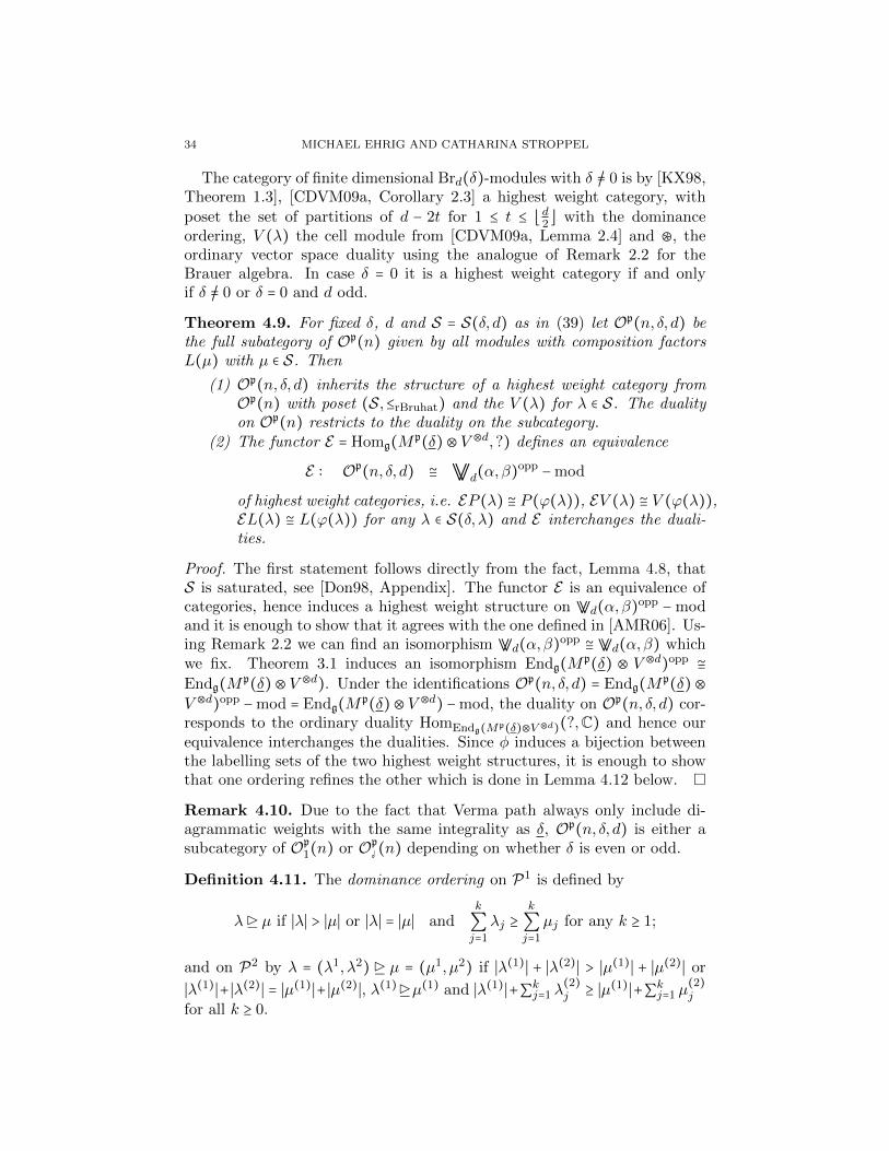
4.3. Quasi-hereditaryness. The category Op(n) is a highest weight cat-egory in the sense of [CPS88], i.e. it is a category C with a poset (S,≤)satisfying
C is an C-linear Artinian category equipped with a duality, that is,a contravariant involutive equivalence of categories ⊛ ∶ C → C;
for each λ ∈ S there is a given object L(λ) ≅ L(λ)⊛ ∈ C such thatL(λ)∣λ ∈ S is a complete set of representatives for the isomorphismclasses of irreducible objects in C;
each L(λ) has a projective cover P (λ) ∈ C such that all compositionfactors of P (λ) are isomorphic to L(µ)’s for µ ∈ S;
writing V (λ) for the largest quotient of P (λ) with the property thatall composition factors of its radical are isomorphic to L(µ)’s forµ > λ, the object P (λ) has a filtration with V (λ) at the top and allother factors isomorphic to V (ν)’s for ν < λ.
The poset S is in our example the set of Λ highest weight vectors forirreducible modules with the reversed Bruhat ordering ≤rBruhat; V (λ) is theVerma module of highest weight λ and the duality is the standard dualityfrom O, [Hum08].
The category ⩔d(α,β)opp − mod of finite dimensional (right) ⩔d(α,β)-
modules is by [AMR06, Corollary 8.6] also a highest weight category, with
poset the set of bipartitions of d − 2t for 1 ≤ t ≤ ⌊d2⌋ equipped with thedominance ordering defined below, V (λ) the cell module from [AMR06,Section 6], and ⊛ the ordinary vector space duality using Remark 2.2.
34 MICHAEL EHRIG AND CATHARINA STROPPEL
The category of finite dimensional Brd(δ)-modules with δ /= 0 is by [KX98,Theorem 1.3], [CDVM09a, Corollary 2.3] a highest weight category, with
poset the set of partitions of d − 2t for 1 ≤ t ≤ ⌊d2⌋ with the dominanceordering, V (λ) the cell module from [CDVM09a, Lemma 2.4] and ⊛, theordinary vector space duality using the analogue of Remark 2.2 for theBrauer algebra. In case δ = 0 it is a highest weight category if and onlyif δ /= 0 or δ = 0 and d odd.
Theorem 4.9. For fixed δ, d and S = S(δ, d) as in (39) let Op(n, δ, d) bethe full subategory of Op(n) given by all modules with composition factorsL(µ) with µ ∈ S. Then
(1) Op(n, δ, d) inherits the structure of a highest weight category fromOp(n) with poset (S,≤rBruhat) and the V (λ) for λ ∈ S. The dualityon Op(n) restricts to the duality on the subcategory.
(2) The functor E = Homg(Mp(δ)⊗ V ⊗d, ?) defines an equivalence
E ∶ Op(n, δ, d) ≅ ⩔d(α,β)
opp−mod
of highest weight categories, i.e. EP (λ) ≅ P (ϕ(λ)), EV (λ) ≅ V (ϕ(λ)),EL(λ) ≅ L(ϕ(λ)) for any λ ∈ S(δ, λ) and E interchanges the duali-ties.
Proof. The first statement follows directly from the fact, Lemma 4.8, thatS is saturated, see [Don98, Appendix]. The functor E is an equivalence ofcategories, hence induces a highest weight structure on ⩔d(α,β)
opp − modand it is enough to show that it agrees with the one defined in [AMR06]. Us-ing Remark 2.2 we can find an isomorphism ⩔d(α,β)
opp ≅ ⩔d(α,β) whichwe fix. Theorem 3.1 induces an isomorphism Endg(M
p(δ) ⊗ V ⊗d)opp ≅
Endg(Mp(δ)⊗ V ⊗d). Under the identifications Op(n, δ, d) = Endg(M
p(δ)⊗
V ⊗d)opp −mod = Endg(Mp(δ)⊗ V ⊗d) −mod, the duality on Op(n, δ, d) cor-
responds to the ordinary duality HomEndg(Mp(δ)⊗V ⊗d)(?,C) and hence ourequivalence interchanges the dualities. Since φ induces a bijection betweenthe labelling sets of the two highest weight structures, it is enough to showthat one ordering refines the other which is done in Lemma 4.12 below.
Remark 4.10. Due to the fact that Verma path always only include di-agrammatic weights with the same integrality as δ, Op(n, δ, d) is either asubcategory of Op
1(n) or Op (n) depending on whether δ is even or odd.
Definition 4.11. The dominance ordering on P1 is defined by
λ µ if ∣λ∣ > ∣µ∣ or ∣λ∣ = ∣µ∣ andk
∑j=1
λj ≥k
∑j=1
µj for any k ≥ 1;
and on P2 by λ = (λ1, λ2) µ = (µ1, µ2) if ∣λ(1)∣ + ∣λ(2)∣ > ∣µ(1)∣ + ∣µ(2)∣ or
∣λ(1)∣+ ∣λ(2)∣ = ∣µ(1)∣+ ∣µ(2)∣, λ(1)µ(1) and ∣λ(1)∣+∑kj=1 λ
(2)j ≥ ∣µ(1)∣+∑
kj=1 µ
(2)j
for all k ≥ 0.
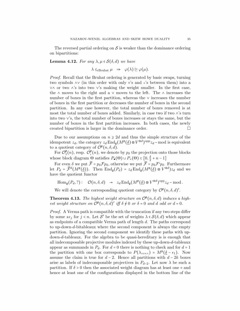
NAZAROV-WENZL ALGEBRAS AND SKEW HOWE DUALITY 35
The reversed partial ordering on S is weaker than the dominance orderingon bipartitions:
Lemma 4.12. For any λ,µ ∈ S(δ, d) we have
λ ≤rBruhat µ ⇒ ϕ(λ) ϕ(µ).
Proof. Recall that the Bruhat ordering is generated by basic swaps, turningtwo symbols ∧∨ (in this order with only ’s and ×’s between them) into a∨∧ or two ∧’s into two ∨’s making the weight smaller. In the first case,the ∧ moves to the right and a ∨ moves to the left. The ∧ increases thenumber of boxes in the first partition, whereas the ∨ increases the numberof boxes in the first partition or decreases the number of boxes in the secondpartition. In any case however, the total number of boxes removed is atmost the total number of boxes added. Similarly, in case two if two ∧’s turninto two ∨’s, the total number of boxes increases or stays the same, but thenumber of boxes in the first partition increases. In both cases, the newlycreated bipartition is larger in the dominance order.
Due to our assumptions on n ≥ 2d and thus the simple structure of theidempotent zd, the category zdEndg(M
p(δ)⊗V ⊗d)oppzd −mod is equivalentto a quotient category of Op(n, δ, d).
For Op1(n), resp. Op
(n), we denote by pδ the projection onto those blocks
whose block diagram Θ satisfies P(Θ) ∪ P×(Θ) ⊂ [0, δ2 + n − 1]
For even δ we put F = pδFpδ, otherwise we put F = pδF pδ. Furthermore
let Pd = Fd(Mp(δ)). Then Endg(Pd) = zdEndg(Mp(δ) ⊗ V ⊗d)zd and we
have the quotient functor
Homg(Pd, ?) ∶ O(n, δ, d) → zdEndg(Mp(δ)⊗ V ⊗d
)oppzd −mod .
We will denote the corresponding quotient category by Op(n, δ, d)′.
Theorem 4.13. The highest weight structure on Op(n, δ, d) induces a high-est weight structure on Op(n, δ, d)′ iff δ /= 0 or δ = 0 and d odd or d = 0.
Proof. A Verma path is compatible with the truncation if any two steps differby some ±εj for j < n. Let S ′ be the set of weights λ ∈ S(δ, d) which appearas endpoints of a compatible Verma path of length d. The paths correspondto up-down-d-bitableaux where the second component is always the emptypartition. Ignoring the second component we identify these paths with up-down-d-tableaux. For the algebra to be quasi-hereditary is is enough thatall indecomposable projective modules indexed by these up-down-d-tableauxappear as summands in Pd. For d = 0 there is nothing to check and for d = 1the partition with one box corresponds to P (λ∧×∧) = Mp(δ − ε1). Nowassume the claim is true for d − 2. Hence all partitions with d − 2k boxesarise as labels of indecomposable projectives in Pd−2. Let now λ be such apartition. If δ > 0 then the associated weight diagram has at least one andhence at least one of the configurations displayed in the bottom line of the
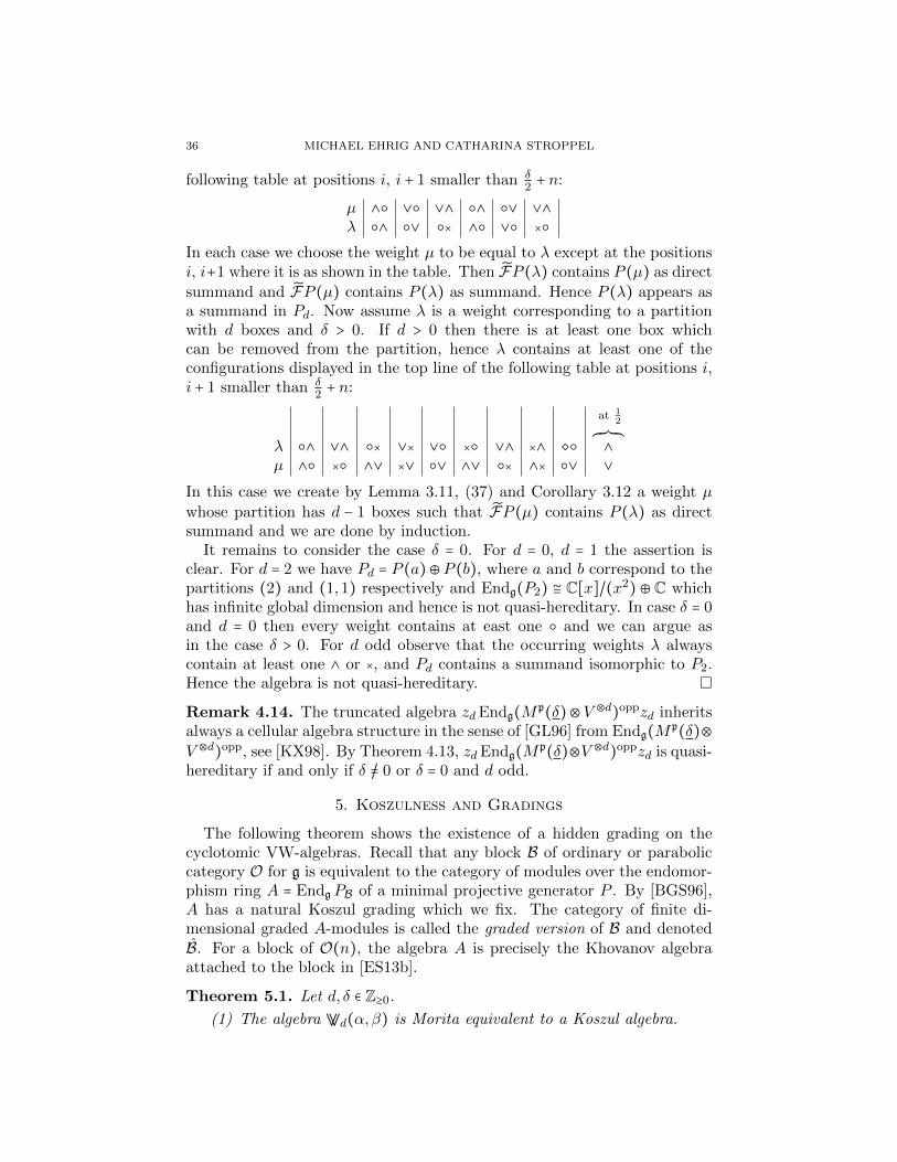
36 MICHAEL EHRIG AND CATHARINA STROPPEL
following table at positions i, i + 1 smaller than δ2 + n:
µ ∧ ∨ ∨∧ ∧ ∨ ∨∧
λ ∧ ∨ × ∧ ∨ ×
In each case we choose the weight µ to be equal to λ except at the positionsi, i+1 where it is as shown in the table. Then FP (λ) contains P (µ) as direct
summand and FP (µ) contains P (λ) as summand. Hence P (λ) appears asa summand in Pd. Now assume λ is a weight corresponding to a partitionwith d boxes and δ > 0. If d > 0 then there is at least one box whichcan be removed from the partition, hence λ contains at least one of theconfigurations displayed in the top line of the following table at positions i,i + 1 smaller than δ
2 + n:
λ ∧ ∨∧ × ∨× ∨ × ∨∧ ×∧
at 12
³·µ∧
µ ∧ × ∧∨ ×∨ ∨ ∧∨ × ∧× ∨ ∨
In this case we create by Lemma 3.11, (37) and Corollary 3.12 a weight µ
whose partition has d − 1 boxes such that FP (µ) contains P (λ) as directsummand and we are done by induction.
It remains to consider the case δ = 0. For d = 0, d = 1 the assertion isclear. For d = 2 we have Pd = P (a)⊕P (b), where a and b correspond to thepartitions (2) and (1,1) respectively and Endg(P2) ≅ C[x]/(x2) ⊕C whichhas infinite global dimension and hence is not quasi-hereditary. In case δ = 0and d = 0 then every weight contains at east one and we can argue asin the case δ > 0. For d odd observe that the occurring weights λ alwayscontain at least one ∧ or ×, and Pd contains a summand isomorphic to P2.Hence the algebra is not quasi-hereditary.
Remark 4.14. The truncated algebra zdEndg(Mp(δ)⊗V ⊗d)oppzd inherits
always a cellular algebra structure in the sense of [GL96] from Endg(Mp(δ)⊗
V ⊗d)opp, see [KX98]. By Theorem 4.13, zdEndg(Mp(δ)⊗V ⊗d)oppzd is quasi-
hereditary if and only if δ /= 0 or δ = 0 and d odd.
5. Koszulness and Gradings
The following theorem shows the existence of a hidden grading on thecyclotomic VW-algebras. Recall that any block B of ordinary or paraboliccategory O for g is equivalent to the category of modules over the endomor-phism ring A = Endg PB of a minimal projective generator P . By [BGS96],A has a natural Koszul grading which we fix. The category of finite di-mensional graded A-modules is called the graded version of B and denotedB. For a block of O(n), the algebra A is precisely the Khovanov algebraattached to the block in [ES13b].
Theorem 5.1. Let d, δ ∈ Z≥0.
(1) The algebra ⩔d(α,β) is Morita equivalent to a Koszul algebra.
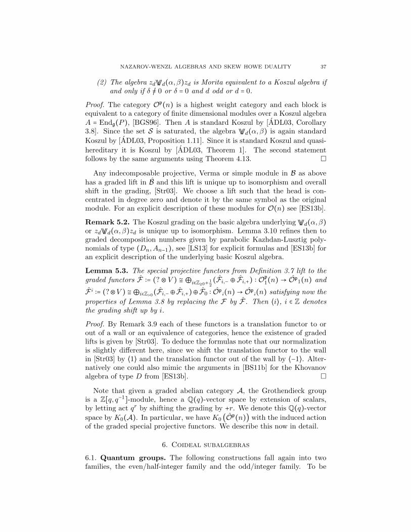
NAZAROV-WENZL ALGEBRAS AND SKEW HOWE DUALITY 37
(2) The algebra zd⩔d(α,β)zd is Morita equivalent to a Koszul algebra ifand only if δ /= 0 or δ = 0 and d odd or d = 0.
Proof. The category Op(n) is a highest weight category and each block isequivalent to a category of finite dimensional modules over a Koszul algebraA = Endg(P ), [BGS96]. Then A is standard Koszul by [ADL03, Corollary3.8]. Since the set S is saturated, the algebra ⩔d(α,β) is again standard
Koszul by [ADL03, Proposition 1.11]. Since it is standard Koszul and quasi-
hereditary it is Koszul by [ADL03, Theorem 1]. The second statementfollows by the same arguments using Theorem 4.13.
Any indecomposable projective, Verma or simple module in B as abovehas a graded lift in B and this lift is unique up to isomorphism and overallshift in the grading, [Str03]. We choose a lift such that the head is con-centrated in degree zero and denote it by the same symbol as the originalmodule. For an explicit description of these modules for O(n) see [ES13b].
Remark 5.2. The Koszul grading on the basic algebra underlying ⩔d(α,β)or zd⩔d(α,β)zd is unique up to isomorphism. Lemma 3.10 refines then tograded decomposition numbers given by parabolic Kazhdan-Lusztig poly-nomials of type (Dn,An−1), see [LS13] for explicit formulas and [ES13b] foran explicit description of the underlying basic Koszul algebra.
Lemma 5.3. The special projective functors from Definition 3.7 lift to thegraded functors F ∶= (? ⊗ V ) ≅ ⊕i∈Z≥0+ 1
2(Fi,− ⊕ Fi,+) ∶ O
p1(n) → O
p1(n) and
F ∶= (?⊗V ) ≅⊕i∈Z>0(Fi,−⊕ Fi,+)⊕ F0 ∶ Op (n)→ Op
(n) satisfying now the
properties of Lemma 3.8 by replacing the F by F . Then ⟨i⟩, i ∈ Z denotesthe grading shift up by i.
Proof. By Remark 3.9 each of these functors is a translation functor to orout of a wall or an equivalence of categories, hence the existence of gradedlifts is given by [Str03]. To deduce the formulas note that our normalizationis slightly different here, since we shift the translation functor to the wallin [Str03] by ⟨1⟩ and the translation functor out of the wall by ⟨−1⟩. Alter-natively one could also mimic the arguments in [BS11b] for the Khovanovalgebra of type D from [ES13b].
Note that given a graded abelian category A, the Grothendieck groupis a Z[q, q−1]-module, hence a Q(q)-vector space by extension of scalars,by letting act qr by shifting the grading by +r. We denote this Q(q)-vector
space by K0(A). In particular, we have K0 (Op(n)) with the induced action
of the graded special projective functors. We describe this now in detail.
6. Coideal subalgebras
6.1. Quantum groups. The following constructions fall again into twofamilies, the even/half-integer family and the odd/integer family. To be
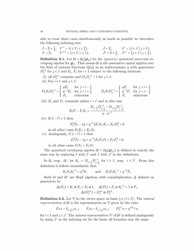
38 MICHAEL EHRIG AND CATHARINA STROPPEL
able to treat these cases simultaneously as much as possible we introducethe following indexing sets:
I = Z + 12 , I++ = i ∈ I ∣ i ≥ 3
2, J = Z, J+ = j ∈ J ∣ j ≥ 1,I = Z, I ,++ = i ∈ I ∣ i ≥ 1, J = Z + 1
2 , J ,+ = j ∈ J ∣ j ≥ 12.
Definition 6.1. Let U = Uq(glZ) be the (generic) quantized universal en-veloping algebra for glZ. That means U is the associative unital algebra overthe field of rational functions Q(q) in an indeterminate q with generatorsD±1j for j ∈ J and Ei, Fi for i ∈ I subject to the following relations:
(i) all D±1j commute and DjD
−1j = 1 for j ∈ J ,
(ii) For i ∈ I and j ∈ J :
DjEiD−1j =
⎧⎪⎪⎪⎨⎪⎪⎪⎩
qEi for j = i − 12
q−1Ei for j = i + 12
Ei otherwiseDjFiD
−1j =
⎧⎪⎪⎪⎨⎪⎪⎪⎩
qFi for j = i + 12
q−1Fi for j = i − 12
Fi otherwise
(iii) Ei and Fi′ commute unless i = i′ and in this case
EiFi − FiEi =Di− 1
2D−1i+ 1
2
−Di+ 12D−1i− 1
2
q − q−1.
(iv) If ∣i − i′∣ = 1 then
E2i Ei′ − (q + q−1
)EiEi′Ei +Ei′E2i = 0
in all other cases EiEi′ = Ei′Ei.(v) Analogously, if ∣i − i′∣ = 1 then
F 2i Fi′ − (q + q−1
)FiFi′Fi + Fi′F2i = 0
in all other cases FiFi′ = Fi′Fi.
The quantized enveloping algebra U = Uq(glZ ) is defined in exactly thesame way by replacing I with I and J with J in the definitions.
In U , resp. U , let Ki ∶= Di− 12D−1i+ 1
2
for i ∈ I, resp. i ∈ I . From this
definition it follows immediately that
KiEiK−1i = q2Ei and KiFiK
−1i = q−2Fi.
Both U and U are Hopf algebras with comultiplication ∆ defined ongenerators by
∆(Ei) =Ki ⊗Ei +Ei ⊗ 1, ∆(Fi) = Fi ⊗K−1i + 1⊗ Fi,
∆(D±1j ) =D±1
j ⊗D±1j .
Definition 6.2. Let V be the vector space on basis vl ∣ l ∈ J. The naturalrepresentation of U is the representation on V given by the rules
Eivl = δi+ 12,lvl−1 Fivl = δi− 1
2,lvl+1 D±1
j vl = q±δj,lvl
for i ∈ I and j ∈ J . The natural representation V of U is defined analogouslyby using J as the indexing set for the basis; all formulas stay the same.
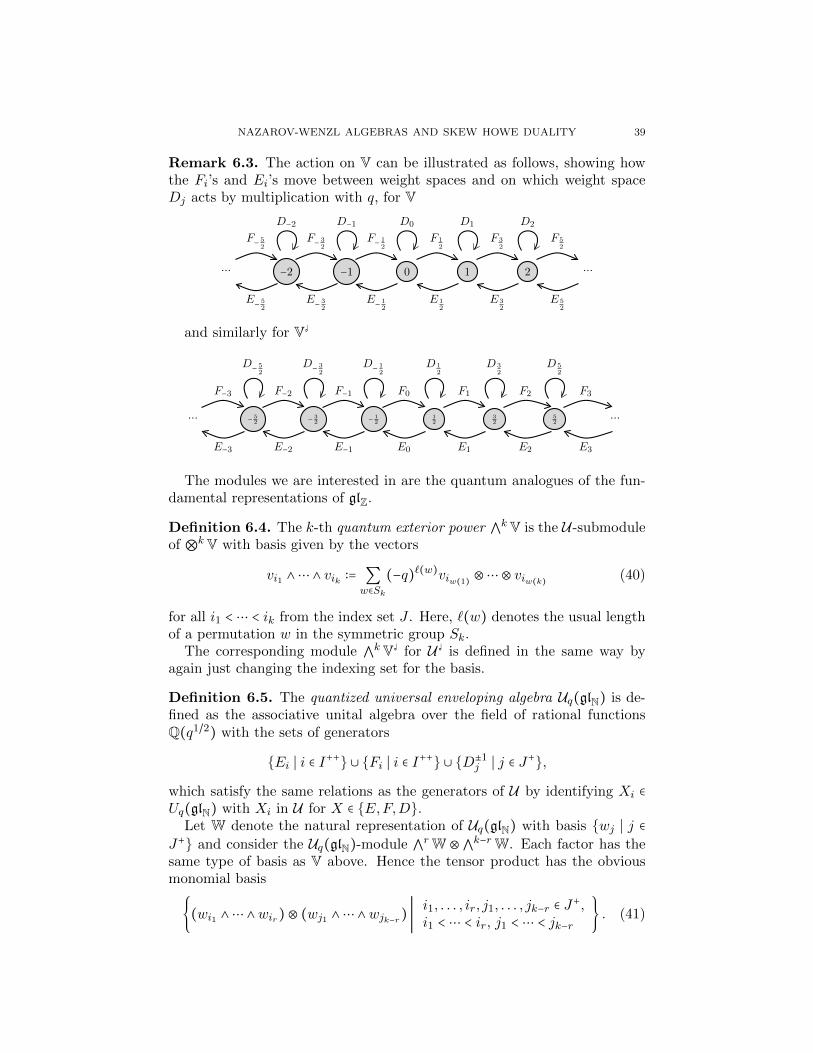
NAZAROV-WENZL ALGEBRAS AND SKEW HOWE DUALITY 39
Remark 6.3. The action on V can be illustrated as follows, showing howthe Fi’s and Ei’s move between weight spaces and on which weight spaceDj acts by multiplication with q, for V
⋯ −2
F− 52
E− 52
D−2
−1
F− 32
E− 32
D−1
0
F− 12
E− 12
D0
1
F 12
E 12
D1
2
F 32
E 32
D2
⋯
F 52
E 52
and similarly for V
⋯ −52
F−3
E−3
D− 52
−32
F−2
E−2
D− 32
−12
F−1
E−1
D− 12
12
F0
E0
D 12
32
F1
E1
D 32
52
F2
E2
D 52
⋯
F3
E3
The modules we are interested in are the quantum analogues of the fun-damental representations of glZ.
Definition 6.4. The k-th quantum exterior power ⋀kV is the U-submoduleof ⊗kV with basis given by the vectors
vi1 ∧⋯ ∧ vik ∶= ∑w∈Sk
(−q)`(w)viw(1) ⊗⋯⊗ viw(k) (40)
for all i1 < ⋯ < ik from the index set J . Here, `(w) denotes the usual lengthof a permutation w in the symmetric group Sk.
The corresponding module ⋀kV for U is defined in the same way byagain just changing the indexing set for the basis.
Definition 6.5. The quantized universal enveloping algebra Uq(glN) is de-fined as the associative unital algebra over the field of rational functionsQ(q1/2) with the sets of generators
Ei ∣ i ∈ I++
∪ Fi ∣ i ∈ I++
∪ D±1j ∣ j ∈ J+,
which satisfy the same relations as the generators of U by identifying Xi ∈
Uq(glN) with Xi in U for X ∈ E,F,D.Let W denote the natural representation of Uq(glN) with basis wj ∣ j ∈
J+ and consider the Uq(glN)-module ⋀rW ⊗⋀k−rW. Each factor has the
same type of basis as V above. Hence the tensor product has the obviousmonomial basis
(wi1 ∧⋯ ∧wir)⊗ (wj1 ∧⋯ ∧wjk−r) ∣i1, . . . , ir, j1, . . . , jk−r ∈ J
+,i1 < ⋯ < ir, j1 < ⋯ < jk−r
. (41)
40 MICHAEL EHRIG AND CATHARINA STROPPEL
As before we can change the indexing set for the generators of Uq(glN) toI ,++ and J ,+ and would obtain an isomorphic algebra with correspondingnatural representation W .
Remark 6.6. Although the above definition of Uq(glN) gives a natural em-bedding of Hopf algebras into both U and U we will be interested in anothercopy of Uq(glN) inside U and U given by certain involution invariant gener-ators.
6.2. Coideal subalgebra. We are interested in the quantization of thefixed point Lie algebra gθ for a certain involution θ. Unfortunately, theobvious construction Uq(g
θ) does not naturally embed into Uq(g). A wayaround this is to study coideal subalgebras (instead of Hopf subalgebras) ofUq(g) which specialize to gθ. This was studied in [Let03] and [Let02].
Lemma 6.7. The assignment
Ei ↦ qK−iF−i, Fi ↦ q−1E−iK−1−i (42)
Dj ↦D−1−j , Ki ↦K−i, q ↦ q−1 (43)
defines a q-antilinear involution θ on both U and U .
Proof. We first note that θ2(X) =X for any generator X, e.g.
θ2(Ei) = θ(qK−iF−i) = q
−1Kiq−1EiK
−1i = Ei.
To see that it is well-defined we have to verify the relations. They fall intothree families of which we check explicitly one each and omit the analogouscalculations. Commuting relations:
θ(Di+ 12EiD
−1i+ 1
2
) =D−1−i− 1
2
qK−iF−iD−i− 12= q2K−iF−i = θ(q
−1Ei).
Commutator relations:
θ(EiFi − FiEi) = K−iF−iE−iK−1−i −E−iF−i
= F−iE−i −E−iF−i = −D−i− 1
2D−1−i+ 1
2
−D−i+ 12D−1−i− 1
2
q − q−1
= θ⎛⎜⎝
Di+ 12D−1i− 1
2
−Di− 12D−1i+ 1
2
q−1 − q
⎞⎟⎠= θ
⎛⎜⎝
Di− 12D−1i+ 1
2
−Di+ 12D−1i− 1
2
q − q−1
⎞⎟⎠,
Quantum Serre relations:
θ (E2i Ei+1 − (q + q−1
)EiEi+1Ei +Ei+1E2i )
= q3K−iF−iK−iF−iK−i−1F−i−1 − (q + q−1)q3K−iF−iK−i−1F−i−1K−iF−i
+q3K−i−1F−i−1K−iF−iK−iF−i
= q3K2−iK−i−1 (F
2−iF−i−1 − (q + q−1
)F−iF−i−1F−i + F−i−1F2−i) = 0
The claim follows.
NAZAROV-WENZL ALGEBRAS AND SKEW HOWE DUALITY 41
To study the fixed points of our involution θ, we enlarge the quantumgroups U and U by also including the elements d±1
j for j ∈ J , resp. j ∈ J ,
satisfying d2j = Dj and corresponding elements ki = di− 1
2d−1i+ 1
2
. The relations
for these elements are the same as for their squares just dividing the powers
of q by two, hence we enlarge the base field to Q(q12 ). Denote these algebras
by U and U respectively.
Lemma 6.8. The involution θ ∶ U → U fixes the following elements Bi ∈ U
Bi = q−12Eik
−1i k
−1−i + q
− 12F−ik−ik
−1i for i ≠ −1
2 ,
B− 12
= E− 12k−1− 1
2
k−112
+ q−1F 12k 1
2k−1− 1
2
.
The involution θ fixes the following elements Bi ∈ U
Bi = q−12Eik
−1i k
−1−i + q
− 12F−ik−ik
−1i for i ≠ 0,
B0 = q−1E0K−10 + F0.
Proof. This is just a straight-forward calculation. For example one checks
θ (q−12Eik
−1i k
−1−i ) = q
32K−iF−ik
−1−i k
−1i = q−
12F−ik−ik
−1i .
Note that the definition of the generators of the coideal subalgebras varyslightly in the literature, see [Let03] and [Let02], although the coideals areclassified. For our purposes a slight renormalisation of the generators ismore suited.
Definition 6.9. We fix the following elements in U
Bi ∶= q12 Bikik
−1−i = EiK
−1−i + F−i for i ≠ ±1
2 ,
B 12∶= q
12 B 1
2k 1
2k−1− 1
2
= E 12K−1− 1
2
+ F− 12,
B− 12∶= qB− 1
2k− 1
2k−1
12
= qE− 12K−1
12
+ F 12.
and also the following elements in U
Bi ∶= q12 Bikik
−1−i = EiK
−1−i + F−i for i ≠ 0,
B0 ∶= B0 = q−1E0K−10 + F0.
Definition 6.10. Let R denote the commutative subalgebra of U generatedby the elements of the form (DjD−j)
±1 for all j ∈ J . Analogously we have R
the commutative subalgebra of U generated by all (DjD−j)±1 for all j ∈ J .
Even though the generators are not invariant under θ it follows from thedefinition that they are mapped to their inverse via θ and thus R and R
themselves are stable under θ.
Remark 6.11. The subalgebras R and R contain the elements of the formKiK
−1−i . They are slightly larger than the commutative subalgebra of the
coideal subalgebra appearing in [Let03], since we are considering gl insteadof sl.
42 MICHAEL EHRIG AND CATHARINA STROPPEL
Definition 6.12. Let H be the subalgebra of U generated by the Bi for i ∈ Iand the subalgebra R. In analogy, let H be the subalgebra of U generatedby the Bi for i ∈ I and the subalgebra R .
The following lemma is straight-forward and checked on generators.
Lemma 6.13. We have ∆(H) ⊂ H ⊗ U , resp. ∆(H ) ⊂ H ⊗ U , hence H,resp. H , is a right coideal subalgebra of U , resp. U .
Remark 6.14. If we truncate our indexing set at m, we obtain the coidealsubalgebra of type AIII discussed in [Let03, Section 7] specializing to theLie subalgebra glm × glm ⊂ gl2m (resp. glm × glm+1). Our renormalisationdoes not change this fact as we only multiplied with elements of the formkik
−1−i . See also Section 7 for fixed point Lie algebras.
Although H and H are not quantum groups, they each contain a copy ofthe quantum group Uq(glN):
Lemma 6.15. The assignment
Ei ↦ Bi, Fi ↦ B−i, D±1j ↦ (DjD−j)
±1 ,
for i ∈ I++ and j ∈ J+ extends to an injective map of algebras from Uq(glN)
to H. We denote the image of this embedding by U .
Proof. Obviously the images of the D±1j ’s are pairwise inverse elements that
form a commutative subalgebra. Furthermore one checks that
DjD−jBi(DjD−j)−1
=
⎧⎪⎪⎪⎨⎪⎪⎪⎩
qBi if j = i − 12
q−1Bi if j = i + 12
Bi otherwise
and that the analogous statement for B−i with inverse q’s holds as well.Computing the commutator we obtain
[Bi,B−i] = [EiK−1−i , Fi] + [F−i,E−iK
−1i ] = [Ei, Fi]K
−1−i + [F−i,E−i]K
−1i
=KiK
−1−i −K−iK
−1i
q − q−1.
and [Bi,B−i′] = 0 if i ≠ i′. It remains to verify the quantum Serre relations,which is a long, but straight-forward calculation and therefore omitted.
Remark 6.16. By using the indexing set I ,++ and J ,+ for Uq(glN) we
obtain the same embedding for H and denote its image by U .
The coideal subalgebras have a Serre type presentation very similar tothe quantum groups except that the Serre relations involving the generatorsB± 1
2and B0 are slightly modified, see [Let03, Theorem 7.1] for a general
statement. In our case we have:
Proposition 6.17. The coideal subalgebra H is isomorphic to the Q(q)-algebra H with generators
Ei, Fi ∣ i ∈ I++
∪ B+, B− ∪ D±1j ∣ j ∈ J+ ∪ D±1
0 ,
NAZAROV-WENZL ALGEBRAS AND SKEW HOWE DUALITY 43
subject to the following relations
(1) The D±1i generate a subalgebra isomorphic to R.
(2) The Ei, Fi, and D±1j for i ∈ I++ and j ∈ J+ generate a subalgebra
isomorphic to Uq(glN).
(3) D0 commutes with Ei and Fi for all i ∈ I++, while B+ and B− com-mute with all other generators except for the following relations(a) Commutation relations:
D1B+D−11 = q−1B+, D1B−D
−11 = qB−
D0B+D−10 = q2B+, D0B−D
−10 = q−2B−
(b) Quantum Serre relations:
B2+E 3
2− (q + q−1
)B+E 32B+ + E 3
2B2+ = 0,
B2−F 3
2− (q + q−1
)B−F 32B− + F 3
2B2− = 0,
E232
B+ − (q + q−1)E 3
2B+E 3
2+ B+E
232
= 0,
F 232
B− − (q + q−1)F 3
2B−F 3
2+ B−F
232
= 0,
(c) Modified quantum Serre relations:
B2+B− − (q + q−1
)B+B−B+ + B−B2+
= −(q + q−1)B+(qD
−11 D0 + q
−1D1D−10 ),
B2−B+ − (q + q−1
)B−B+B− + B+B2−
= −(q + q−1)B−(q
2D1D−10 + q−2D−1
1 D0).
Proof. Up to renormalization these are the relations from [Let03] for thecoideal subalgebra of type AIII. The isomorphism is then given by Ei ↦ Bi,Fi ↦ B−i, D
±1j ↦ (DjD−j)
±1 , and B+ ↦ B 12, B− ↦ B− 1
2, D0 ↦D2
0.
An analogous statement also holds for H .
Proposition 6.18. The coideal subalgebra H is isomorphic to the Q(q)-algebra H with generators
Ei, Fi ∣ i ∈ I ,++
∪ B ∪ D±1j ∣ j ∈ J ,+
,
subject to the following relations
(1) The D±1i generate a subalgebra isomorphic to R .
(2) The Ei, Fi, and D±1j for i ∈ I ,++ and j ∈ J ,+ generate a subalgebra
isomorphic to Uq(glN).
(3) The generator B commutes with all other generators except for thefollowing relations:
E21B − (q + q−1
)E1BE1 + BE21 = 0,
F 21 B − (q + q−1
)F1BF1 + BF21 = 0,
44 MICHAEL EHRIG AND CATHARINA STROPPEL
B2E1 − (q + q−1)BE1B + E1B
2= E1,
B2F1 − (q + q−1)BF1B + F1B
2= F1.
6.3. Action on ⋀nV. In [BS11a], a calculus of diagrammatic weights and
diagrammatic algebras was introduced to describe maximal parabolic ver-sions of the BGG-category O in type A. In particular, the Grothendieckgroup of the maximal parabolic category O was identified with the Q(q)-vector space over the basis of diagrammatic weights which in turn was identi-fied with a module for the quantum group Uq(glZ). Here we like to developan analogous picture (based on [ES13b]). The first step is to decomposespecific U-modules with respect to U .
For a sequence i = (i1 < . . . < ir) of strictly decreasing integers we denoteby i+ the subsequence of strictly positive numbers, by i− the subsequence ofstrictly negative numbers and by i0 the subsequence consisting of the entryequal to 0 if they exists, otherwise they are empty. Furthermore we denoteby −i the sequence (−ir < . . . < −i1).
Lemma 6.19. There is an isomorphism of Uq(glN)-modules
Φ ∶n
⋀VÐ→n
⊕r=0
(r
⋀W⊗n−r
⋀ W)⊕n−1
⊕r=0
(r
⋀W⊗Q(q)⊗n−1−r
⋀ W)
where Uq(glN) acts on the left via the isomorphism with U and Q(q) is thetrivial representation with basis w0. The map is given by
Φ(vi) = w−i− ⊗wi0 ⊗wi+ if i0 ≠ ∅,w−i− ⊗wi+ otherwise.
Similarly, there is an isomorphism of Uq(glN)-modules
Φ ∶n
⋀V Ð→
n
⊕r=0
(r
⋀W ⊗n−r
⋀ W ) ,
where Uq(glN) acts on the left via the isomorphism with U and the map isgiven by Φ (vi) = w−i− ⊗wi+ .
Proof. We will omit the proof since the second isomorphism is a special caseof Lemma 6.20 and the first completely analogous.
The following more general decomposition will be used in Section 7.
Lemma 6.20. Let r ∈ Z≥1 and k1, . . . , kr ∈ Z≥1. We have an isomorphismof Uq(glN)-modules
Φ ∶k1
⋀V ⊗. . .⊗
kr
⋀V Ð→ ⊕
0≤si≤ki
(kr−sr
⋀ W ⊗ . . .⊗
k1−s1
⋀ W ⊗
s1
⋀W ⊗ . . .⊗
sr
⋀W ) ,
where Uq(glN) acts on the left via the isomorphism with U followed by thecomultiplication of U and the map is given by
Φ (vi1 ⊗ . . .⊗ vir) = w−ir,− ⊗ . . .⊗w−i1,− ⊗wi1,+ ⊗ . . .⊗wir,+ .
NAZAROV-WENZL ALGEBRAS AND SKEW HOWE DUALITY 45
Proof. The map is an isomorphism of vector spaces since it sends a basis to abasis and both spaces have the same dimension. We need to verify that it isUq(glN)-linear. We will only check the linearity on generators Ea for a ∈ I ,++,since the arguments for the others are parallel. On the left hand side, Ea actsvia the isomorphism, which maps Ea to Ba followed by successive applicationof the comultiplication. Hence Ea acts by multiplication with
r−1
∑l=0
(KaK−1−a)
⊗l⊗EaK
−1−a ⊗ (K−1
−a)⊗(r−1−l)
+r−1
∑l=0
1⊗l ⊗ F−a ⊗ (K−1−a)
⊗(r−1−l).
If we denote by d(i, a) and d(i,−a) the integers such that
Kavi = qd(i,a)vi, K−avi = q
−d(i,−a)vi.
for a vector v = vi = vi1 ⊗ . . .⊗ vir , then we get
Ea.v =r−1
∑l=0
1⊗l ⊗Ea ⊗ 1⊗(r−1−l).v ⋅ qd(i1,−a)+...+d(ir,−a)qd(i1,a)+...+d(il,a)
+r−1
∑l=0
1⊗l ⊗ F−a ⊗ 1⊗(r−1−l).v ⋅ qd(il+2,−a)+...+d(ir,−a).
On the other hand w ∶= Φ (v) = w−ir,− ⊗ . . .⊗w−i1,− ⊗wi1,+ ⊗ . . .⊗wir,+ . Since
Kawi+ = qd(i,a)wi+ Kaw−ii = q
d(i,−a)w−i−
for Ka ∈ Uq(glZ) and any sequence i we obtain
Ea.w =r−1
∑l=0
1⊗l ⊗Ea ⊗ 1⊗(2r−1−l).w ⋅ qd(ir,−a)+...+d(ir−l+1,−a)
+2r−1
∑l=r
1⊗l ⊗Ea ⊗ 1⊗(2r−1−l).w ⋅ qd(ir,−a)+...+d(i1,−a)qd(i1,a)+...+d(il−r,a)
=r−1
∑l=0
1⊗(r−1−l)⊗Ea ⊗ 1⊗(r+l).w ⋅ qd(ir,−a)+...+d(il+2,−a)
+r−1
∑l=0
1⊗(r+l)⊗Ea ⊗ 1⊗(r−1−l).w ⋅ qd(ir,−a)+...+d(i1,−a)qd(i1,a)+...+d(il,a).
In the last step we just reordered the first sum and shifted the indexingof the second. In particular, Φ commutes with the action of Ea. Simi-lar calculations for the other generators imply that Φ is a Uq(glN)-modulehomomorphism.
Using the identification of K0 (Op1(n)), resp. K0 (O
p (n)), with the Q(q)-
vector spaces having Xn, resp. X n, as basis we can identify our modules
with these spaces.Integer case: Consider the Uq(glN)-module ⋀nV. To a standard basis
vector vi we can assign a diagrammatic weight in Xn via defining the sets
46 MICHAEL EHRIG AND CATHARINA STROPPEL
P∨(i) = ij ∣ ij > 0, P∧(i) = −ij ∣ ij < 0 and P(i) = ij ∣ ij = 0. The map
Γ ∶n
⋀VÐ→K0 (Op1(n)) ,
defined on bases vectors by
Γ(vi)l ∶=
⎧⎪⎪⎪⎪⎪⎪⎪⎨⎪⎪⎪⎪⎪⎪⎪⎩
∨ if l ∈ P∨(i) ∖ P∧(i),∧ if l ∈ P∧(i) ∖ P∨(i), if l ∈ P(i),× if l ∈ P∧(i) ∩ P∨(i), if l /∈ P∧(i) ∪ P∨(i) ∪ P(i).
yields an isomorphism of vector spaces. For a diagrammatic weight λ wedenote the corresponding standard basis vector by vλ.
Half-integer case: Consider the Uq(glN)-module ⋀nV . To a standardbasis vector vi we again assign a diagrammatic weight, this time in X
n viadefining the sets P∨(i) = ij ∣ ij > 0 and P∧(i) = −ij ∣ ij < 0. The map
Γ ∶n
⋀V Ð→K0 (O
p (n)) ,
defined on basis vectors by
Γ (vi)l ∶=
⎧⎪⎪⎪⎪⎪⎨⎪⎪⎪⎪⎪⎩
∨ if l ∈ P∨(i) ∖ P∧(i),∧ if l ∈ P∧(i) ∖ P∨(i),× if l ∈ P∧(i) ∩ P∨(i), if l /∈ P∧(i) ∪ P∨(i).
yields an isomorphism of vector spaces. Again we denote the preimage of adiagrammatic weight λ by vλ.
Using these two isomorphisms Γ and Γ we can transfer the action of U andU to the vector spaces of diagrammatic weights. In general the generatorsof U and U will not act in a way that is compatible with the structureof the categories underlying these vector spaces, but we will see that thegenerators of H and H act in a way that can be interpreted categoricallyas the induced action of translation functors. The following Lemmas are allproved by a straightforward case by case calculation.
Lemma 6.21. Let λ be a diagrammatic weight, then
DjD−jλ =
⎧⎪⎪⎪⎨⎪⎪⎪⎩
λ if λj = ,qλ if λj ∈ ∨,∧,q2λ if λj = ×.
Lemma 6.22. Let λ be a diagrammatic weight in Xn and i ∈ I++. Forsymbols x, y ∈ ,∧,∨,× we write λxy for the diagrammatic weight obtained
from λ by relabelling the (i − 12)th entry to x and the (i + 1
2)th entry to y.
(1) We first consider the action of Bi:(i) If λ = λ∨, then Bi.λ = λ∨.
(ii) If λ = λ∧, then Bi.λ = λ∧.(iii) If λ = λ∧×, then Bi.λ = λ×∧.(iv) If λ = λ∨×, then Bi.λ = λ×∨.
NAZAROV-WENZL ALGEBRAS AND SKEW HOWE DUALITY 47
(v) If λ = λ∧∨, then Bi.λ = qλ×.(vi) If λ = λ∨∧, then Bi.λ = λ×.
(vii) If λ = λ×, then Bi.λ = q−1λ∨∧ + λ∧∨.
(viii) For all other λ we have Bi.λ = 0.(2) We now consider the action of B−i:
(i) If λ = λ∧, then B−i.λ = λ∧.(ii) If λ = λ∨, then B−i.λ = λ∨.
(iii) If λ = λ×∨, then B−i.λ = λ∨×.(iv) If λ = λ×∧, then B−i.λ = λ∧×.(v) If λ = λ∧∨, then B−i.λ = qλ×.
(vi) If λ = λ∨∧, then B−i.λ = λ×.(vii) If λ = λ×, then B−i.λ = q
−1λ∨∧ + λ∧∨.(viii) For all other λ we have B−i.λ = 0.
Remark 6.23. The analogous version of Lemma 6.22 also holds if we lookat diagrammatic weights in X and i ∈ I ,++, i.e replace X by X and I++ byI ,++ in the statements.
With Lemmas 6.21 and 6.22 we know the action of the generators Ei, Fi,and D±1
i of H and H induced on K0 (Op(n)) and K0 (O
p (n)) for i ∈ I++
and i ∈ I ,++. We consider the action of the special generators B0, B− 12.
Lemma 6.24. (1) The element B0 acts by zero on a diagrammatic weightλ ∈ X
n unless λ 12∈ ∧,∨. If λ = λ∨ then B0.λ = λ∧ and if λ = λ∧
then B0.λ = λ∨.(2) Let λ ∈ Xn. For symbols x, y ∈ ,∧,∨,×, we write λxy for the
diagrammatic weight obtained from λ by relabelling the 0th entry tox and the 1st entry to y.
(i+) If λ = λ∨ then B 12.λ = λ.
(ii+) If λ = λ∧ then B 12.λ = λ.
(iii+) If λ = λ× then B 12.λ = q−1λ∧ + λ∨.
(iv+) For all other λ we have B 12.λ = 0.
(i-) If λ = λ then B− 12.λ = λ∧ + λ∨.
(ii-) If λ = λ∨ then B− 12.λ = qλ×.
(iii-) If λ = λ∧ then B− 12.λ = λ×.
(iv-) For all other λ we have B− 12.λ = 0.
By comparing the actions of Bi on diagrammatic weights with the inducedaction of translation functors we obtain the following result.
Proposition 6.25. On K0 (Op1(n)), the induced action of B±i and B± 1
2on
K0 via Γ coincides with the action of [Fi,±] and [F 12,±] respectively. On
K0 (Op (n)), the induced action of B±i and B0 on K0 via Γ coincides with
the action of [Fi,±] and [F 12,±] respectively.
48 MICHAEL EHRIG AND CATHARINA STROPPEL
Proof. This follows by comparing the action as described in Lemma 6.22and Lemma 6.24 with the description of the action of the special translationfunctors Fi,± on Verma modules in Lemma 3.8.
6.4. Bar involution and dual canonical basis. We start by defining aninvolution on H and H . In generalizes Lusztig’s bar involution to coideals.
Lemma 6.26. There is a unique Q(q)-antilinear bar-involution − ∶ H → H
such that Bi = Bi and DjD−j =D−1j D
−1−j ; similar for H .
Proof. Using Proposition 6.17 one checks easily that such an assignmentextends to an algebra involution.
Definition 6.27. By a compatible bar-involution on an H-module M wemean an anti-linear involution − ∶ M → M such that uv = uv for eachu ∈H, v ∈M and analogously for a H -module.
Note that as a U-module V has one-dimensional weight spaces with allstandard basis vectors being weight vectors. The next lemma shows that themodule ⋀nV possesses a compatible bar-involution. As our identification ofthe action of H and the translation functors already indicates, we will needto focus on vectors wλ that correspond to a diagrammatic weight λ. Recallthat for two diagrammatic weights in the same block ΛεΘ we have the Bruhatorder which gives a unique minimal element in each block. As usual, we startwith the case of diagrammatic weights supported on the integers.
Lemma 6.28. There is a unique compatible bar-involution on the H-module
⋀nV such that wλ = wλ for each diagrammatic weight λ ∈ X that is minimal
in its block with respect to the Bruhat order. Moreover:
wλ ∈ wλ + ∑µ<λ
q−1Z[q−1]wµ,
for any λ ∈ X.
Proof. We prove uniqueness, the existence follows below from Lemma 6.30.For any diagrammatic weight λ let l(λ) denote the height of the weight inthe reversed Bruhat order, i.e. the minimal number of changes that need tomade to obtain the minimal element as described in [ES13b, Lemma 2.3].
Enough to show: wλ is uniquely determined by the properties. For λminimal wλ = wλ, hence it is determined. So let us fix λ non-minimal andassume that wµ is uniquely determined for all µ with l(µ) < l(λ). Note thatthis includes diagrammatic weights in other blocks.
Case I: Assume there exists i < j such that λi = ∧ and λj = ∨ andλs ∈ ,× for i < s < j. Let λ′ be the diagrammatic weight that coincideswith λ except for λ′i+1 = ∨ and λ′s = λs−1 for i+ 1 < s ≤ j, i.e. we have movedthe ∨ at position j next to the ∧ at position i. By Lemma 6.22 it followsthat there exists B ∈ H such that Bwλ′ = wλ. Furthermore let µ be thediagrammatic weight that coincides with λ′ except the positions i and i + 1
NAZAROV-WENZL ALGEBRAS AND SKEW HOWE DUALITY 49
are swapped, then l(µ) < l(λ′) = l(λ). Then it follows again by Lemma 6.22that
B−i− 12Bi+ 1
2.wµ = q
−1wµ +wλ′ .
This implies
wλ = BB−i− 12Bi+ 1
2.wµ − qBwµ.
Hence wλ is uniquely determined.Case II: Assume there is no pair i < j as in Case I, then there exists
i < j such that λi ∈ ∨, and λj = ∨ and choose i and j minimal with thisproperty. As before we can always assume that j = i + 1 since there can beno ∧’s between i and j by assumption.
If i = 0 let µ be the weight sequence coinciding with λ except µ1 = ∧.Then by Lemma 2
B 12B− 1
2(wµ) = q
−1wµ +wλ.
Again this implies
wλ = B 12B− 1
2(wµ) − qwµ.
If on the other hand i ≠ 0 then move the symbols at position i and i+1 toposition 0 and 1, denote the corresponding weight by η. By the calculationabove we already know
wη = B 12B− 1
2(wµ) − qwµ,
where µ coincides with η except that µ1 = ∧. We can now use the elementB′ ∈H that first moves the symbols at position 1 back to position i + 1 andafterwards the symbol at position 0 back to position i and obtain
B′wη = B′B 1
2B− 1
2(wµ) − qB
′wµ,
since l(µ) < l(λ) the right hand side is known, but
B′wη = wλ +wλ′ ,
with λ′ coinciding with λ except λ′i = ∧. Since l(λ′) = l(λ) we can useCase I to deduce that wλ′ is already determined and hence wλ is uniquelydetermined.
Lemma 6.29. There is a unique compatible bar-involution on the H -module
⋀nV such that wλ = wλ for each diagrammatic weight λ ∈ X that is minimal
in its block with respect to the Bruhat order. Moreover:
wλ ∈ wλ + ∑µ<λ
q−1Z[q−1]wµ,
for any λ ∈ X .
Proof. The uniqueness of a bar-involution on the H -module ⋀nV followswith similar arguments to Lemma 6.28, although they are slightly simplerbecause the special generator B0 behaves nicer. The details are left to thereader.
50 MICHAEL EHRIG AND CATHARINA STROPPEL
For the existence of a bar-involution with these properties we use that
⋀nV ≅ K0 (O
p1(n)) and that there is a graded duality on Op
1(n) satisfyingthese properties.
Proposition 6.30. The graded duality d on Op1(n), sending a module M to
M, induces a compatible bar-involution on ⋀nV, satisfying the propertiesof Lemma 6.28. The same also holds for the graded duality on Op
(n) andthe induced involution on ⋀nV .
Proof. Let M(λ) be a parabolic Verma module corresponding to a diagram-matic weight being minimal in its block. Then M(λ) = L(λ) and hence
dM(λ) = dL(λ) = L(λ) =M(λ).
If on the other hand M(λ) is a Verma module corresponding to an arbi-trary diagrammatic weight, we have that dM(λ) =M(λ) = ∇(λ), the dualparabolic Verma module by definition. It is known, see [Str03] that
[∇(λ)] ∈ [M(λ)] + ∑µ<λ
q−1Z[q−1][M(µ)].
It remains to show that d is compatible with the action of H.Since the simple modules form a basis of the Grothendieck group it is
enough to check the compatibility on those, i.e. we need to show that fora translation functor F corresponding to a generator of H and any simplemodule L(λ) we have
[FL(λ)] = [FdL(λ)] = [dFL(λ)],
where the first equality is due to the fact that simple modules are self-dual.Thus we need to show that [FL(λ)] is self-dual as well. We will focus onFi,+ and leave the other cases to the reader. Using Lemma 3.8 we know that
Fi,+L(λ∨) = L(λ∨) Fi,+L(λ∧) = 0,
Fi,+L(λ∧×) = L(λ×∧) Fi,+L(λ∨×) = 0,
Fi,+L(λ∧∨) = 0 Fi,+L(λ∨∧) = L(λ×).
All of these are obviously self-dual and we are left with the case where Fi,+is applied to a weight λ = λ×. This is done by showing that
[Fi,+L(λ×)] = q[L(λ∨∧)] + [L(λ∧∨)] + q−1
[L(λ∨∧)],
which is self-dual. Let Y be a set of diagrammatic weights and rµ and sµintegers such that
[L(λ×)] = ∑µ∈Y
(−1)rµqsµ[M(µ)],
then for all these µ we have µ = µ×. Applying Lemma 6.22 we obtain
[Fi,+L(λ×)] = ∑µ∈Y
(−1)rµqsµ−1[M(µ∨∧)] + (−1)rµqsµ[M(µ∧∨)]
= q−1∑µ∈Y
(−1)rµqsµ[M(µ∨∧)]
NAZAROV-WENZL ALGEBRAS AND SKEW HOWE DUALITY 51
+ ∑µ∈Y
(−1)rµ (qsµ[M(µ∧∨)] − qsµ+1
[M(µ∨∧)])
+q ∑µ∈Y
(−1)rµqsµ[M(µ∨∧)].
Expressing [L(λ∨∧)], and [L(λ∧∨)] in terms of Verma modules one checksthat this is equal to (q + q−1)[L(λ∨∧)] + [L(λ∧∨)].
Note that the isomorphism classes of simple modules concentrated in de-gree zero form a canonical basis of ⋀nV ≅ K0 (O
p1(n)), that is they are
bar-invariant and the transformation matrix to the standard basis is lowerdiagonal with 1’s in the diagonal and elements in Z[q] below the diago-nal. These entries are the parabolic Kazhdan-Lusztig polynomials of type(Dn,An−1).
7. Skew Howe duality
In the following we want to look at more general versions of parabolic cat-egory O of type D and correspondingly categorifications of tensor productsas in Lemma 6.20 for Uq(glZ) and H. Since the quantum parameter in thesecases is very technical we will work first in the classical case and considercategorifications of glr × glr-modules, instead of H-modules.
7.1. The module ⋀(n,m, r). For a positive integer t we denote by W t
the vector space of dimension t with basis v 12, . . . , vt− 1
2, with basis elements
labelled by half-integers. Similarly we denote by V 2k the vector space of di-
mension 2t with basis v−t+ 12, . . . , vt− 1
2. Finally denote by M the 2-dimensional
vector space with basis v+ and v−. Depending on the situation we will regardthese as vector spaces over C or over Q(q), in which case they are truncationof the spaces W and V we had in Section 6.
In the following fix m and r positive integers. We want to consider modulestructures on the vector space
⋀(n,m, r) ∶=n
⋀ (W m ⊗M⊗W
r) .
Since one can identify W m ⊗ M ≃ V
2m and M ⊗ W r ≃ V
2r we can view
⋀(n,m, r) natural both as a (gl2m,glr)-bimodule and a (glm,gl2r)-bimodule.
7.2. Fixed point subalgebra. We first identify the fixed point subalgebraof gl2m which is the non-quantized analogue of H. The classical analogueof the involution from Lemma 6.7 is Θ ∶ gl2m → gl2m defined as A ↦ JAJ ,
where J = (0 JJ 0
) with J as in Section 2. i.e has 1’s on the anti-diagonal
and zeros elsewhere. Then
gΘ= X ∈ gl2m ∣ JXJ =X with J = (
0 JJ 0
) ,
52 MICHAEL EHRIG AND CATHARINA STROPPEL
We have gΘ ≅ glm × glm, since it is the image of the involution
TA ∶ gl2m Ð→ gl2m, X ↦ AXA−1 with A = (1 JJ −1
) ,
where 1 is the m×m identity matrix. Restricted to glm×glm, let gl+m and gl−mdenote the images of the first respectively second factor one easily verifies,
using JA = A(1 00 −1
) and AJ = (1 00 −1
)A, that
gl+m = (X XJJX JXJ
) X ∈ glm and (44)
gl−m = (X −XJ
−JX JXJ) X ∈ glm . (45)
Fix the identification W m⊗M ≃ V
2m, vi⊗v+ ↦ vi and vi⊗v− ↦ v−i as vectorspaces. Twisting with TA gives the decomposition
V 2m =W
m ⊗ ⟨v+ + v−⟩⊕W m ⊗ ⟨v+ − v−⟩ , (46)
as a gΘ = gl+m × gl−m-module. One should note that gl+m acts as zero onthe second summand, while gl−m acts as zero on the first summand. Thediagonally embedded glm in glm × glm with its Chevalley generators normal-ized by 1
2 maps via TA to an isomorphic subalgebra of gl2m with generatorsEi ∶= Ei+1,i + E−i−1,−i and Fi ∶= Ei,i+1 + E−i,−i−1 for 0 < i < m. These areexactly the specialization of the generators Bi and B−i from Definition 6.9.Together with the specialization of R they generate the diagonally embed-ded glm in gl+m × gl−m. The special generator B0 specializes to the elementG = E1,−1 + E−1,1 and generates together with the diagonal embedded Lie
algebra the whole fixed point Lie algebra gΘ.
7.3. The classical and quantum skew Howe duality. All the identifi-cations made above can of course also be done for gl2r and we will use thesame notations for them. Using the decomposition from (46) we obtain
⋀(n,m, r) =n
⋀ (W m ⊗ ⟨v+ + v−⟩⊗W
r ⊕W m ⊗ ⟨v+ − v−⟩⊗W
r) (47)
≃n
⊕i=0
i
⋀ (W m ⊗ ⟨v+ + v−⟩⊗W
r)⊗n−i
⋀ (W m ⊗ ⟨v+ − v−⟩⊗W
r)
≃n
⊕i=0
i
⋀ (W m ⊗ ⟨v+ + v−⟩⊗W
r) ⊠n−i
⋀ (W m ⊗ ⟨v+ − v−⟩⊗W
r) ,
where the ⊠ should denote that we regard the first factor as a (gl+m,gl+r )-
bimodule and the second as a (gl−m,gl−r )-bimodule and take the outer tensor
product of these two bimodules in each summand. From the usual skewHowe duality of glm and glr on ⋀n(W
m ⊗W r) we can deduce that on each
summand the gl+m × gl−m-endomorphisms are generated by gl+r × gl−r and that
there are no such morphisms between different summands. We obtain
NAZAROV-WENZL ALGEBRAS AND SKEW HOWE DUALITY 53
Theorem 7.1. The actions of U(gl+m ×gl−m) and U(gl+r ×gl−r ) on ⋀(n,m, r)
commute and generate each others commutant.
7.4. The categorified classical skew Howe duality. To categorify thebimodule ⋀(n,m, r) we first use classical skew Howe duality for the pair(gl2m,glr) to obtain a decomposition as gl2m-module
⋀(n,m, r) ≅ ⊕k∈C(n,r)
k
⋀V m,
where C(n, r) denotes the set of composition of n with r parts and ⋀kV m =
⋀k1 V
m ⊗ . . . ⊗ ⋀kr V m. Naturally each summand is also a module for the
subalgebra gl+m × gl−m. To identify each summand with the Grothendieckgroup of certain blocks of parabolic category O we denote by pk the standardparabolic of so2n corresponding to the root subsystem where we omit thesimple roots
α0, αk1 , αk1+k2 , αk1+k2+k3 , . . . , αk1+...+kr−1 ,
for each choice of k ∈ C(n, r). In this language our original parabolic p = p(n).
As in Section 1 we have the corresponding parabolic category Opk(n)inside the full category O. For the basis of the corresponding Grothendieckgroups, we have to look at pk-dominant weights.
Definition 7.2. An integral weight λ is pk-dominant if it is of the form
λ = (λ1 ≤ . . . ≤ λk1 , λk1+1 ≤ . . . ≤ λk1+k2 , . . . , λk1+...+kr−1+1 ≤ . . . ≤ λn).
Let Λk denote the set of all pk-dominant weights, decomposing as usual into
Λk = Λ1k ∪Λ
k, depending on whether the λi’s are integers or half-integers.
Consider the subcategoryOpk≤m(n) generated by simple modules with high-
est weight in
Λ≤mk = λ ∈ Λ
k ∣ ∣λi + ρi∣ ≤m −1
2 .
This is obviously a finite set and stable under the dot-action of the Weyl
group, thus Opk≤m(n) is a finite sum of certain blocks in O
pk≤m(n). In complete
analogy to Section 6, we associate to λ ∈ Λ≤mk a vector vλ ∈ ⋀
kV m in the
following way. First denote λ′ = λ + ρ, then consider the sequence
ijλ = (λ′k1+...+kj > λ′k1+...+kj−1 > . . . > λ
′k1+...+kj−1+1),
and define the corresponding standard basis vector as vλ = vi1λ⊗ . . . ⊗ virλ .
Then [Mpk(λ)]↦ vλ defines an isomorphism of vector spaces
Γk ∶ K0 (Opk≤m(n))Ð→
k
⋀V m.
Taking (direct) sums we obtain
Γm ∶ K0⎛
⎝⊕
k∈C(n,r)
Opk≤m(n)
⎞
⎠Ð→⋀(n,m, r). (48)
54 MICHAEL EHRIG AND CATHARINA STROPPEL
Alternatively we could look at the decomposition as gl2r-module and get
Γr ∶ K0⎛
⎝⊕
k∈C(n,m)
Opk≤r(n)
⎞
⎠Ð→⋀(n,m, r). (49)
Next, we decompose the categories Opk≤m(n). Although we will refer to this
as a block decomposition, this is not completely correct as the subcategoriesmight decompose further, but it is a decomposition by central character.
Remark 7.3. Note that two pk-dominant weights give rise to parabolicVerma modules with the same central character iff they are in the same Weylgroup orbit with respect to the dot-action. After adding ρ this correspondsto usual Weyl group orbits. Then two weights lie in the same orbit iff themultiplicity for each half-integer 1
2 , . . . ,m − 12 , up to sign, agrees in the two
weights and the multiplicities of negative integers have the same parity.
Definition 7.4. Let (k,µ, ε) be two compositions of n, k with at most r
non-trivial parts and µ with at most m non-trivial parts and ε ∈ 0,1 a
parity. Then O(k,µ,ε)(n), will denote the subcategory of Opk≤m(n) such that
all weights λ of parabolic Verma modules appearing satisfy
# j ∣ λj + ρj ∣= i −12
= µi and # j λj + ρi < 0 = ε.
Let us denote by Bl(n, r,m) the set of all triples (k,µ, ε) as above, calledblock triples. Then we define, for a block triple Γ, the projection
prΓ ∶ Opk≤m → OΓ(n).
For 1 ≤ i ≤m − 1 and a block triple Γ = (k,µ, ε) we define the triples
Γi,+ = (k,µ′, ε) via µ′l =
⎧⎪⎪⎪⎪⎨⎪⎪⎪⎪⎩
µl − 1 if l = i + 1
µl + 1 if l = i
µl otherwise,
(50)
Γi,− = (k,µ′, ε) via µ′l =
⎧⎪⎪⎪⎪⎨⎪⎪⎪⎪⎩
µl + 1 if l = i + 1
µl − 1 if l = i
µl otherwise,
(51)
and
Γ0 = (k,µ, ε + 1). (52)
Generalizing Definition 3.7 we can now define certain translation functors.
Definition 7.5. We have the special projective functors Fi,+, Fi,− for i ∈ Z≥0
and F0 defined by
Fi,− ∶=⊕Γ
prΓi,− (?⊗ V ) prΓ ∶ ⊕Γ
OΓ(n)→⊕Γ
OΓ(n),
Fi,+ ∶=⊕Γ
prΓi,+ (?⊗ V ) prΓ ∶ ⊕Γ
OΓ(n)→⊕Γ
OΓ(n),
NAZAROV-WENZL ALGEBRAS AND SKEW HOWE DUALITY 55
F0 ∶=⊕Γ
prΓ0(?⊗ V ) prΓ ∶ ⊕
Γ
OΓ(n)→⊕Γ
OΓ(n),
with all sums running over Γ ∈ Bl(n, r,m).
Proposition 7.6. Under the identification
K0⎛
⎝⊕
Γ∈Bl(n,r,m)
OΓ(n)⎞
⎠=⋀(n,m, r)
the action of [Fi,−] coincides with the one of Fi, the action of [Fi,+] coincideswith the one of Ei and the action of [F0] coincides with the action of G,hence gives a categorification of the action of gl+m × gl−m.
Proof. We show the claim for Fi,+ and leave the rest to the reader. LetΓ = (k,µ, ε) be a block triple andMpk(λ) be a parabolic Verma module in the
corresponding block. Then we can express Mpk(λ)⊗V in the Grothendieckgroup as
[Mpk(λ)⊗ V ] = ∑l∶λ+εl∈Λk
[Mpk(λ + εl)] + ∑l∶λ−εl∈Λk
[Mpk(λ − εl)].
Checking now when a parabolic Verma module of the form Mpk(λ − εl) liesin the block corresponding to Γi,+ we see that this is the case if and only if
λl + ρl = i +12 and similarly with Mpk(λ + εl). Under our identification this
coincides exactly with the way Ei acts on the Grothendieck group.
7.5. The commuting action of the Hecke algebra. As before we re-strict to the half-integer case. Consider the special case where k = (1,1, . . . ,1),
hence ⋀kV m = V
m⊗r.
Definition 7.7. The Hecke algebra Hr corresponding to the Weyl groupWr = ⟨sαi ∣ 0 ≤ i ≤ r⟩ of so2r is the unital Q(q)-algebra with generators Hi,0 ≤ i ≤ r subject to the quadratic relation H2
i = 1+ (q−1 − q)Hi, and the typeD braid relations HiHj = HjHi if sαisαj = sαjsαi and HiHjHi = HjHiHj ifsαisαjsαi = sαjsαisαj with 1 ≤ i, j ≤ r.
Lemma 7.8. There is a right action of the Hecke algebra Hr on V m⊗r
commuting with the action of H . The generator Hi for 1 ≤ i ≤ r acts on theith and i + 1th tensor factor by the formula
va ⊗ vb.Hi =
⎧⎪⎪⎪⎪⎨⎪⎪⎪⎪⎩
vb ⊗ va if a < b
vb ⊗ va + (q−1 − q)va ⊗ vb if a > b
q−1vb ⊗ va if a = b.
(53)
and H0 acts on the first and second tensor factor by
va ⊗ vb.H0 =
⎧⎪⎪⎪⎪⎨⎪⎪⎪⎪⎩
v−b ⊗ v−a if (55) holds,
v−b ⊗ v−a + (q−1 − q)va ⊗ vb if (56) holds
q−1v−b ⊗ v−a if a = −b,
(54)
for a, b > 0, or (∣a∣ > ∣b∣ and b < 0 < a), or (∣a∣ < ∣b∣ and a < 0 < b); (55)

56 MICHAEL EHRIG AND CATHARINA STROPPEL
for a, b < 0, or (∣a∣ > ∣b∣ and a < 0 < b), or (∣a∣ < ∣b∣ and b < 0 < a). (56)
Proof. One can directly verify that the rules are compatible with the re-lations in the Hecke algebra, hence indeed define an action. The verifica-tion that it commutes with the action of the coideal subalgebra is a lengthystraight forward case by case calculation showing that (Bj .v).Hi = Bj .(v.Hi)
for any choice of j, i and basis vector v.
Analogously we can identify ⋀(n,m, r) with K0 (⊕Γ∈Bl(n,m,r)OΓ(n)) and
with the analogous functors obtain an action of gl+r × gl−r .
Consider the graded version Opk≤m(n) of O
pk≤m(n) as described in Section 5.
We again have the corresponding identification of Q(q)-vector spaces
Γk ∶ K0 (Opk≤m(n))Ð→
k
⋀V m. (57)
by sending the class [Mpk(λ)] of the standard graded lift of the parabolicVerma module Mpk(λ) to vλ with head concentrated in degree zero. (Themultiplication with q corresponds to the grading shift ⟨1⟩).
Recall from [AL03], [AS03] the right exact twisting endofunctors Ti ∶= Tsαiof the integral category O attached to sαi . Their left derived functors defineauto-equivalences of the derived category. The Hecke algebra action has acategorification given by graded lifts of these derived functors:
Proposition 7.9. Let k = (1,1, . . . ,1). Then the derived functor LTi, 0 ≤
i ≤ n − 1 has a graded lift,
LTi ∶ Db(O
pk≤m(n))→Db
(Opk≤m(n)), (58)
an automorphism of the bounded derived category Db(Opk≤m(n)) such that the
induced action of LTi on K0(Db(O
pk≤m(n))) = K0(O
pk≤m(n)) agrees with the
action of the Hecke algebra generator Hi under the identification Γk.
Proof. If we forget the grading this is [AL03, 2.1]. The graded version is[FKS06, Propositions 5.1 and 5.2].
We like to extend the categorification from Proposition 7.6 to the quantumcase. We first have to give an alternative description of the special functors.Recall from [BG80], [Hum08] the definition and classification of translationon and out of walls. Given integral weights λ,µ with corresponding blockOλ(n) and Oµ(n) let Wn(λ), Wn(µ) be their stabilizer under the dot-actionof the Weyl group. Assume Wn(λ) ⊂Wn(µ) then we have the translation toand the translation out of the walls functors
θµλ ∶ Oλ(n)→ Oµ(n)
θλµ ∶ Oµ(n)→ Oλ(n).
We are in particular interested in the case, where Wn(µ) differs from Wn(λ)by one additional simple reflection sαi . We call the corresponding functorsthen translation to the ith wall and from the ith wall and denote them by
NAZAROV-WENZL ALGEBRAS AND SKEW HOWE DUALITY 57
θon,i, and θout,i respectively. To make formulas easier we abuse notationand also write θon,i and θout,i in case Wn(µ) =Wn(λ) in which case the twotranslation functors are just inverse equivalences, [Hum08, 7.8].
For 0 ≤ i ≤ m − 1 and a block triple Γ = ((1,1, . . . ,1), µ, ε) we define the
compositions µ↑,i, µ↓,i, where
µ↑,il
=
⎧⎪⎪⎪⎪⎨⎪⎪⎪⎪⎩
µl−1 if l > i + 1,
0 if l = i + 1,
µl if l < i + 1,
µ↓,il
=
⎧⎪⎪⎨⎪⎪⎩
µl+1 if l ≥ i + 1,
µl if l < i + 1,
and Γ↑,i = ((1,1, . . . ,1), µ↑,i, ε), Γ↓,i = ((1,1, . . . ,1), µ↓,i, ε) and consider thecomposition of functors:
Bi,+,Γ ∶ OΓ(n)η→ OΓ1
θout,i+1→ OΓ2
θon,i→ OΓ3
η→ OΓ4 , (59)
where Γ1 = Γ↑,i, Γ2 = (Γ1)i+1,+, Γ3 = (Γ2)i,+, and Γ4 = (Γ3)↓,i = (Γ1)i,+, using
Definition, (50). The η’s stand for the translation functors indicated by theblocks. Since by [Hum08, 7.8] these are equivalences of categories we justdenote them by η. Note that these equivalences exists, since the blocks onlydepends on the singularity type of the corresponding highest weights. Let
Bi,−,Γ4 ∶ OΓ4
η−1→ OΓ3
θout,i→ OΓ2
θon,i+1→ OΓ1
η−1→ OΓ, (60)
be the adjoint functor. We set Bi,+ = ⊕ΓBi,+,Γ and Bi,− = ⊕ΓBi,−,Γ for i > 0and B0 = ⊕Γ(B0,+,Γ ⊕B0,−,Γ) in analogy to Definition 7.5.
Example 7.10. For instance if µ = (0,2,2,2,2) and i = 2 then for Bi we
start at the block k = (1,1, . . . ,1) which is equivalent to (k, (0,2,0,2,2,2), ε),then translate out of the third wall to get to (k, (0,2,1,1,2,2), ε) followed bytranslating to the second wall which ends in (k, (0,3,0,1,2,2), ε). Applyingagain an equivalence we end in (k, (0,3,1,2,2,2), ε), hence we reduced thenumbers of 3’s and increased the number of 2’s.
Lemma 7.11. There are isomorphisms Bi,± ≅ Fi,± for i ≥ 0 and B0 ≅ F0.
Proof. Recall from [BG80] that projective functors, i.e. direct summandsof endofunctors on O(n) given by taking the tensor product with finite di-mensional modules are determined up to isomorphism already by their valueon the Verma modules whose weight is maximal in their dot-orbit of Wn.Hence to prove the lemma it is enough to compare the value on these Vermamodules. Since such a Verma module is a projective object it is enough tocompare their values in the Grothendieck group. We explain this for Bi,+and B0, the case Bi,− is similar. Consider a block Γ = ((1,1, . . . ,1), µ, ε) withcorresponding maximal weight λ such that
λ + ρ = (1, . . . ,1´¹¹¹¹¹¹¹¹¹¸¹¹¹¹¹¹¹¹¹
µ1
, . . . , n, . . . , n´¹¹¹¹¹¹¹¹¹¹¸¹¹¹¹¹¹¹¹¹¹¹
µn
) − (12 , . . . ,
12)
58 MICHAEL EHRIG AND CATHARINA STROPPEL
in case ε = 0 and with the first occurring number negated if ε = 1. Forinstance (2,2,2,3,3,3,4,4) respectively (−2,2,2,3,3,3,4,4) are examples.Now fix first i > 0 and consider Bi,+. Applying the equivalence η sendsM(λ) to M(λ↑,i), where λ↑,i is obtained from λ by changing the numberswith absolute value ≥ (i + 1) by 1 if positive and by −1 if negative.
In our examples above we obtain for instance for i = 2 the highest weightλ↑,2 (up to the shift by ρ and 1
2 in each coordinate) of Verma modules as
(2,2,2,4,4,4,5,5) respectively (−2,2,2,4,4,4,5,5).
Translation out of the (i + 1)th wall gives a module which has a Vermaflag with Verma subquotients precisely the M(ν − ρ) for ν obtained fromλ↑,i by changing exactly one i + 2 to i + 1, [Hum08, 7.12]. In our exam-ple we get for ν exactly the weights (2,2,2,4,4,3,5,5), (2,2,2,4,3,4,5,5),(2,2,2,3,4,4,5,5) for ε = 0 and (−2,2,2,4,4,3,5,5), (−2,2,2,4,3,4,5,5),(−2,2,2,3,4,4,5,5) for ε = 1. Translation to the ith wall maps each Vermamodule M(ν − ρ) to a Verma module M(ν′ − ρ), where ν′ is obtained fromν by changing the unique number i+ 1 into i, [Hum08, 7.6]. In our examplewe get the three highest weights (again without the shifts)
(2,2,2,4,4,2,5,5), (2,2,2,4,2,4,5,5), (2,2,2,2,4,4,5,5)
in case ε = 0 and
(−2,2,2,4,4,2,5,5), (−2,2,2,4,2,4,5,5), (−2,2,2,2,4,4,5,5)
in case ε = 1. The final equivalence just rescales again and we obtain
(2,2,2,3,3,2,4,4), (2,2,2,3,2,3,4,4), (2,2,2,2,3,3,4,4)
respectively
(−2,2,2,3,3,2,4,4), (−2,2,2,3,2,3,4,4), (−2,2,2,2,3,3,4,4).
Comparing with Proposition 7.6 we see this agrees with the values for Fi,±,hence Fi,+ ≅ Bi,+. In case i = 0 we first increase all numbers in absolutevalue by 1, keeping their signs. For instance (1,1,1,2,2) gives (2,2,2,3,3)and (−1,1,1,2,2) gives (−2,2,2,3,3). Then we translate out of the 1th wallif ε = 1 and out of the 0th wall if ε = 0. In our examples we obtain the threehighest weights ν (up to ρ and shift by 1
2) equal to (2,2,1,3,3), (2,1,2,3,3),(1,2,2,3,3) respectively (2,2,−1,3,3), (2,−1,2,3,3), (−1,2,2,3,3). Apply-ing the translation to the 0th respectively 1th wall we obtain Vermas of high-est weights (1,1,1,3,3), (1,1,1,3,3), (1,1,1,3,3) respectively (−1,1,1,3,3),(−1,1,1,3,3), (−1,1,1,3,3). Applying the last equivalence gives the desiredresult and hence B0 ≅ F0.
7.6. Graded translation functors. By [Str03], the translation functorsto and out of a wall θon,i ∶ Oλ(n) → Oµ(n), θout,i ∶ Oλ(n) → Oµ(n) have
NAZAROV-WENZL ALGEBRAS AND SKEW HOWE DUALITY 59
graded lifts, that means can be lifted to graded functors2
θon,i ∶ Oλ(n)Ð→ Oµ(n), θout,i ∶ Oµ(n)Ð→ Oλ(n). (61)
By [BG80], the functors θon,i, and θout,i are indecomposable, hence a gradedlift is unique up to isomorphism and overall shift in the grading, [Str03,Lemma 1.5]. We fix graded lifts θon,i, θout,i such that the graded version ofthe Verma module with maximal weight in the orbit is sent to a projectivemodule with head concentrated in degree zero. We define graded lifts of thefunctors in (59) and (60) by setting for i > 0:
Bi,+,Γ ∶= (η θon,i ˆθout, i + 1 η)⟨µi−1 − µi + 1⟩ (62)
Bi,−,Γ ∶= (η θon,i ˆθout, i + 1 η)⟨µi+1 − µi + 1⟩ (63)
and Bi = ⊕ΓBi,+,Γ and B−i = ⊕ΓBi,−,Γ, where ⟨r⟩, r ∈ Z, means that thegrading is shifted by adding r to the degree. For i = 0 we set
B0 ∶= ⊕Γ(η θon,1 ˆθout,0 η)⊕ (η θon,0 θout,1 η). (64)
These functors induce functors on Opk≤m(n) and then via the identification
(57) Q(q)-linear endomorphisms on the Q(q)-vector space ⋀(n,m, r). Ourmain result here is the following categorification theorem
Theorem 7.12. Under the identification
K0⎛
⎝⊕
Γ∈Bl(n,r,m)
OΓ(n)⎞
⎠=⋀(n,m, r)
as Q(q)-vector space, the action induced from the exact functor Bi coincideswith the action of Bi ∈H
for any i ∈ Z.
We start with the following main insight:
Lemma 7.13. Theorem 7.12 is true when restricted to V m⊗r
.
Proof. It is enough to verify that the action of [Bi] agrees with the actionof Bi ∈ H
on the standard basis corresponding to isomorphism classes ofgraded lifts of Verma modules. Recall the commuting action of the Heckealgebra from Lemma 7.8 and note that twisting functors commute withtranslation functors, [AS03, Theorem 3.2]. Hence by Proposition 7.9 it isenough to compare the action for Verma modules whose highest weight λis maximal in their dot-orbit. Moreover by linearity we can restrict our-selves to the case of standard graded lifts M(λ). We follow the proof of
Lemma 7.11. Consider first the functors Bi for i > 0. The equivalence η liftsto the graded setting and just renames the highest weight of M(λ). Thetranslation out of the wall produces an indecomposable projective moduleP , [Hum08, 7.11] with a graded Verma flag. The Verma subquotients are,
2The arguments about the existence in [Str03] are only for the principal block, butgeneralize directly to arbitrary integral blocks by taking invariants of the coinvariants.
60 MICHAEL EHRIG AND CATHARINA STROPPEL
up to some grading shifts, the M(ν − ρ) with the same weights ν as be-fore. Amongst them let ν(r) be the weight where the rth i + 2 from the
left has been changed. By our normalization, M(ν(rmax)− ρ) with r = rmax
maximal occurs without grading shift and hence P ≅ P (ν(rmax) − ρ). By[BGS96, Theorem 3.11.4], the graded multiplicities are encoded in parabolicKazhdan-Lusztig polynomials. Our case corresponds to the explicit formula[Soe97, Proposition 2.9] and we obtain that P has a filtration with subquo-
tients M(ν(r)−ρ)⟨rmax−r⟩. In our example we get [M((2,2,2,4,4,3,5,5)−
ρ)] + q[M((2,2,2,4,3,4,5,5) − ρ)] + q2[M((2,2,2,3,4,4,5,5) − ρ)] in theGrothendieck group. Now translation to the wall just changes the num-bers i + 1 appearing in the weights to i without any extra grading shiftby [Str03, Theorem 8.1]. The last step is a graded equivalence renam-
ing the weights. In our example we obtain [M((2,2,2,3,3,2,4,4) − ρ)] +
q[M((2,2,2,3,2,3,4,4) − ρ)] + q2[M((2,2,2,2,3,3,4,4) − ρ)]. In any case,the result agrees with the action of Bi up to an overall grading shift by⟨µi−1 −µi + 1⟩. In case i = 0 the arguments are completely parallel except ofthe grading shift at the end. As above, the lowest grading shift appearing forVerma modules is zero. Expressing B0vλ in the standard basis, the smallestq power appearing equals (−1) + n1 − n−1 + (n−1 − n1 + 1) = 0, where nj isthe number of j’s appearing in the weight λ. Hence the claim of the Lemmafollows for B0. For B−i, i > 0 the arguments are analogous.
Proof of Theorem 7.12. Let i > 0. Recall from (40) that the action of Bi onsome standard basis vector v = vi1 ⊗ . . .⊗vir ∈ ⋀
k1 V ⊗ . . .⊗⋀kr V from (41)can be obtained by viewing v as a vector inside ⊗k1 V ⊗ . . . ⊗⊗kr V andcompute the action there. Let [Mpk(µ)] be the class of the standard lift ofthe parabolic Verma module attached to v. Assume first that the stabilizerof µ is trivial under the dot-action and write µ = x ⋅λ with λ maximal in thesame dot-orbit and x ∈Wn. Recall that by definition the Levi subalgebra ofpk is of type A with Weyl group isomorphic to the product Sk of symmetricgroups. Then
[Mpk(µ)] = [Mpk(x ⋅ λ)] = ∑y∈Sk
(−q)`(w)[M(yx ⋅ λ)] (65)
by the formula [Soe97, Proposition 3.4] for parabolic Kazhdan-Lusztig poly-nomials together with [Str05, Corollary 2.5]. This however fits preciselywith the formula (40) and the claim follows. Assume now that the stabilizerW (µ) of µ is not trivial under the dot-action. Then choose λ′ an integralweight, maximal in its dot-orbit and with W (λ′) trivial. Following [Str03]
choose a graded lift θµλ′ of θµλ′ such that θλλ′M(λ′) ≅ M(λ). We claim that
θλλ′M(x ⋅ λ′) ≅ M(x ⋅ λ) (66)
for any shortest coset representative x ∈Wn/W (λ). Since this is true if weforget the grading and M(x ⋅λ) is indecomposable we only have to figure outpossible overall grading shifts, [Str03, Lemma 1.5]. If x is the identity we
NAZAROV-WENZL ALGEBRAS AND SKEW HOWE DUALITY 61
are done by convention. Otherwise we find a simple reflection sαi such that`(sαix) < `(x) and use again that twisting functors, even graded, commutewith translation functors. From Lemma 7.8 and Proposition 7.9 the resultfollows then by induction on `(x). This implies θλλ′M
pk(x ⋅ λ′) ≅ Mpk(x ⋅ λ),since this is again true up to a possible overall shift in the grading which ishowever zero by (66). Moreover, we can choose λ′ such that yx is of minimallength in its coset for any y ∈ Sk. (In practice we consider λ + ρ and replaceits entries by a strictly increasing sequence of positive integers. We do thisby replacing first the lowest numbers from the left to right, then replace thesecond lowest from the left to right etc.) Now we apply [θµλ′] to (65) andobtain with (66)
[Mpk(x ⋅ λ)] = ∑y∈Sk
(−q)`(w)[M(yx ⋅ λ)] (67)
The claim follows then from (40) and Lemma 7.13.
For the block triple Γ = (k,µ, ε) ∈ Bl(n, r,m) we associate the transposed
block triple Γ∨ = (µ, k, nε) ∈ Bl(n,m, r). In other words, the parabolic typeis flipped with the type of the singularity and the parity is kept if n is evenand swapped if n is odd.
Theorem 7.14. Let Γ ∈ Bl(n, r,m) then OΓ(n) is Koszul dual to OΓ∨(n).
Proof. We first recall the description of the Koszul dual block in generalfollowing [Bac99]. Assume we have a blockOIJ of categoryO for any complexsemisimple Lie algebra, where the parabolic is given by a subset I of thesimple roots and the stabilizer of the highest weights of the parabolic Vermamodules are generated by simple reflections given by a subset J of simpleroots. Then the Koszul dual is the block OJI′ , where I ′ = −w0(I) with w0
the longest element in the Weyl group, [Bac99, Theorem 1.1]. In our case oftype Dn, we have −w0(I) = I if n is even and −w0(I) is the set obtained fromI by applying the unique nontrivial diagram automorphism of the Dynkindiagram. Hence the Koszul dual of Γ = (k,µ,0) is the block (µ, k,0) if
n is even and equal to (µ, k,1) in case n is odd; and the Koszul dual of
Γ = (k,µ,1) is the block (µ, k,1) if n is even and equal to (µ, k,0) if n isodd.
Koszul duality, [BGS96], defines an equivalence of categories
Db(OΓ(n)) ≅D
b(OΓ∨(n))
sending Mpk(x ⋅ µ) to Mpµ(x−1w0 ⋅ λ), where µ and λ are maximal weightsin the corresponding dot-orbits of the Weyl group. This duality and itsconnection to the quantum exterior powers can be nicely encoded in termsof box diagrams.
Given Mpk(x ⋅ µ) consider the weight x ⋅ µ + ρ = (µ1, µ2, . . . , µn). This isstrictly increasing in the r parts given by k. Assign to this weight a box
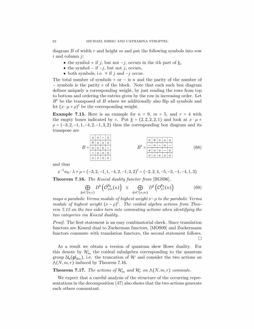
62 MICHAEL EHRIG AND CATHARINA STROPPEL
diagram B of width r and height m and put the following symbols into rowi and column j:
the symbol + if j, but not −j, occurs in the ith part of k, the symbol − if −j, but not j, occurs, both symbols, i.e. ∓ if j and −j occur.
The total number of symbols + or − is n and the parity of the number of− symbols is the parity ε of the block. Note that each such box diagramdefines uniquely a corresponding weight, by just reading the rows from topto bottom and ordering the entries given by the row in increasing order. LetBt be the transposed of B where we additionally also flip all symbols andlet (x ⋅ µ + ρ)t be the corresponding weight.
Example 7.15. Here is an example for n = 9, m = 5, and r = 4 withthe empty boxes indicated by . Put k = (2,2,2,2,1) and look at x ⋅ µ +ρ = (−3,2,−1,1,−4,2,−1,3,2) then the corresponding box diagram and itstranspose are
B =
+ −
∓
+ −
− +
+
Bt=
∓ +
− − −
+ −
+
(68)
and thus
x−1w0 ⋅ λ + ρ = (−3,2,−1,1,−4,2,−1,3,2)t = (−2,2,4,−5,−3,−1,−4,1,3)
Theorem 7.16. The Koszul duality functor from [BGS96],
⊕k∈C(n,r)
Db(O
pk≤m(n)) ≅ ⊕
k∈C(n,m)
Db(O
pk≤r(n)) (69)
maps a parabolic Verma module of highest weight ν−ρ to the parabolic Vermamodule of highest weight (ν − ρ)t. The coideal algebra actions from Theo-rem 7.12 on the two sides turn into commuting actions when identifying thetwo categories via Koszul duality.
Proof. The first statement is an easy combinatorial check. Since translationfunctors are Koszul dual to Zuckerman functors, [MOS09] and Zuckermannfunctors commute with translation functors, the second statement follows.
As a result we obtain a version of quantum skew Howe duality. Forthis denote by H
m the coideal subalgebra corresponding to the quantumgroup Uq(gl2m), i.e. the truncation of H and consider the two actions on
⋀(N,m, r) induced by Theorem 7.16.
Theorem 7.17. The actions of H m and H
r on ⋀(N,m, r) commute.
We expect that a careful analysis of the structure of the occurring repre-sentations in the decomposition (47) also shows that the two actions generateeach others commutant.
NAZAROV-WENZL ALGEBRAS AND SKEW HOWE DUALITY 63
8. Appendix
8.1. Proof of 2.8. This subsection is devoted to the proof of Theorem 2.8.
Lemma 8.1. For 1 ≤ i ≤ d − 1 and j /∈ i, i + 1 we have siyj = yjsi.
Proof. The case j < i is obvious by definition. For the case j > i+ 1 we havefor v ∈M ⊗ V ⊗d:
siyj(v) = si⎛
⎝
⎛
⎝∑
0≤k<j
Ωkj +2n − 1
2
⎞
⎠v⎞
⎠= ∑
0≤k<j
si (Ωkjv) +2n − 1
2si(v)
=⎛
⎝∑
0≤k<j
Ωkj
⎞
⎠si(v) +
2n − 1
2si(v) = yjsi(v).
The claim follows.
The following are the Brauer algebra relations, see e.g. [GW09, Lemma10.1.5]:
Lemma 8.2. For 1 ≤ i ≤ d− 2, the relations eisi = ei = siei, siei+1ei = si+1ei,ei+1eisi+1 = ei+1si, and ei+1eiei+1 = ei+1 hold.
Proof. The first equality is obvious by definition of the map τ . We will onlyproof the second one, the final two are shown analogously. To shorten thenotations we will assume that our morphisms si, ei, and ei+1 only live ona threefold tensor product, with the first factor being the position i, thesecond i + 1, and the third i + 2. Let a, b, c ∈ I and v = va ⊗ vb ⊗ vc, then
(si+1ei).v = ⟨va, vb⟩∑k∈I
vk ⊗ vc ⊗ vk
and
(siei+1ei).v = (siei+1)(⟨va, vb⟩∑k∈I
vk ⊗ v∗k ⊗ vc) = ⟨va, vb⟩∑
k∈I
vk ⊗ vc ⊗ v∗k .
and the claim follows.
Lemma 8.3. For 1 ≤ i ≤ d − 1 we have siyi − yi+1si = ei − 1.
Proof. Since si is invertible it is equivalent to show yi − siyi+1si = ei − si byLemma8.2. Note that siyi+1si equals
si ( ∑0≤k<i+1
Ωki + (2n − 1
2Id)) si = ( ∑
0≤k<i
Ωki + siΩi(i+1)si + (2n − 1
2Id))
Therefore, yi − siyi+1si = −siΩi(i+1)si = −Ωi(i+1) = ei − si, where the lastequality follows from Remark 2.6.
The proofs of the following identities rely on the explicit form of Ω andits action on V ⊗ V .
Lemma 8.4. For 1 ≤ i, j ≤ d − 1 and j /∈ i, i + 1 we have eiyj = yjei.
64 MICHAEL EHRIG AND CATHARINA STROPPEL
Proof. As in Lemma 8.1 the case j < i is obvious by definition and we areleft with the case j > i + 1. The essential part that we need to prove is
(Ωij +Ω(i+1)j) ei = ei (Ωij +Ω(i+1)j) , (70)
since ei naturally commutes with all other summands of yj . Again, wepretend that Ωij , Ω(i+1)j , and ei act only on a threefold tensor product,corresponding to the factors at position i, i + 1 and j.
Consider first the left hand side. Since we first apply ei, the element eiyjkills all basis vectors except the ones of the form x = va ⊗ v
∗a ⊗ vc for some
a, c ∈ I, in which case x.ei = ∑k∈I vk ⊗ v∗k ⊗ vc. and applying Ωij + Ω(i+1)j
gives
∑α∈Bn
∑k∈I
(Xαvk ⊗ v∗k + v
∗k ⊗Xαvk)⊗X
∗αvc
= ∑α∈Bn
∑k∈I
∑l∈I
(⟨Xαvk, vl⟩ v∗l ⊗ v
∗k + v
∗k ⊗ ⟨Xαvk, vl⟩ v
∗l )⊗X
∗αvc
= ∑α∈Bn
∑k,l∈I
(⟨Xαvk, vl⟩ v∗l ⊗ v
∗k − ⟨Xαvl, vk⟩ v
∗k ⊗ v
∗l )⊗X
∗αvc
= 0
Thus (Ωij +Ω(i+1)j) ei = 0 on M ⊗ V ⊗d.Consider now the right hand side of (70), let x = va⊗ vb⊗ vc for a, b, c ∈ I,
then
x.(Ωij +Ω(i+1)j) = ∑α∈Bn
(Xαva ⊗ vb + va ⊗Xαvb)⊗X∗αvc
= ∑α∈Bn,k∈I
(⟨Xαva, vk⟩ v∗k ⊗ vb + ⟨Xαvb, vk⟩ va ⊗ v
∗k)⊗X
∗αvc
Applying ei kills, for fixed α, all except one summand and we obtain
∑l∈I
(⟨Xαva, vb⟩ vl ⊗ v∗l + ⟨Xαvb, va⟩ vl ⊗ v
∗l )⊗X
∗αvc
= ∑l∈I
(⟨Xαva, vb⟩ vl ⊗ v∗l − ⟨Xαva, vb⟩ vl ⊗ v
∗l )⊗X
∗αvc = 0.
Thus, ei (Ωij +Ω(i+1)j) = 0 on M ⊗ V ⊗d and the lemma follows.
Lemma 8.5. For 1 ≤ i, j ≤ d we have yiyj = yjyi.
Proof. We show this by using the following statements:
(i) [Ωij ,Ωkl] = 0 for pairwise different i, j, k, l,(ii) [Ωij +Ωjk,Ωik] = 0 for pairwise different i, j, k.
Equality (i) is obvious. To show (ii) we consider the i-th, j-th and k-thfactor in V ⊗d and calculate
[Ωij +Ωjk,Ωik] = ∑α,β,γ∈Bn
[Xα ⊗X∗α ⊗ 1 + 1⊗Xβ ⊗X
∗β ,Xγ ⊗ 1⊗X∗
γ ]
= ∑α,β,γ∈Bn
[Xα,Xγ]⊗X∗α ⊗X
∗γ +Xγ ⊗Xβ ⊗ [X∗
β ,X∗γ ]
NAZAROV-WENZL ALGEBRAS AND SKEW HOWE DUALITY 65
= ∑α,β,γ,µ∈Bn
([Xα,Xγ],X∗µ)Xµ ⊗X
∗α ⊗X
∗γ
+ ∑α,β,γ,µ∈Bn
Xγ ⊗Xβ ⊗ ([X∗β ,X
∗γ ],Xµ)X
∗µ
(1)= ∑
α,β,γ,µ∈Bn
([Xα,Xγ],X∗µ)Xµ ⊗X
∗α ⊗X
∗γ
+ ∑α,β,γ,µ∈Bn
([X∗α,X
∗µ],Xγ)Xµ ⊗Xα ⊗X
∗γ
(2)= ∑
α,β,γ,µ∈Bn
([Xα,Xγ],X∗µ)Xµ ⊗X
∗α ⊗X
∗γ
− ∑α,β,γ,µ∈Bn
([Xα,Xγ],X∗µ)Xµ ⊗X
∗α ⊗X
∗γ = 0
Here equality (1) is just a relabelling in the second sum and extractinga scalar factor, while equality (2) follows from the invariance of the Killingform, i.e.
∑α∈Bn
([X∗α,X
∗µ],Xγ)Xα = ∑
α∈Bn
(X∗α, [X
∗µ ,Xγ])Xα = ∑
α∈Bn
(Xα, [X∗µ ,Xγ])X
∗α
= − ∑α∈Bn
([Xα,Xγ],X∗µ)X
∗α.
Lemma 8.6. For 1 ≤ 1 < d we have
ei(yi + yi+1) = 0 and (yi + yi+1)ei = 0.
Proof. We start with the first relation and expand the left hand side.
ei(yi + yi+1) = ei ( ∑0≤k<i
(Ωki +Ωk(i+1)) +Ωi(i+1) +N − 1)
= ei ( ∑0≤k<i
(Ωki +Ωk(i+1)) + si − ei +N − 1)
= ei ( ∑0≤k<i
(Ωki +Ωk(i+1))) + ei −Nei + (N − 1)ei
= ei ( ∑0≤k<i
(Ωki +Ωk(i+1)))
We have seen in the proof of Lemma 8.4 that ei (Ωki +Ωk(i+1)) acts as zero
if k > 0. Thus we are left to show that ei (Ω0i +Ω0(i+1)) acts as zero. Letx = m ⊗ va ⊗ vb for m ∈ M and a, b ∈ I, again these should be thought ofpositions 0, i, and i + 1. Applying (Ω0i +Ω0(i+1)) gives us
x. (Ω0i +Ω0(i+1))
66 MICHAEL EHRIG AND CATHARINA STROPPEL
= ∑α∈Bn
Xαm⊗X∗αva ⊗ vb +Xαm⊗ va ⊗X
∗αvb
= ∑α∈Bn
∑k∈I
⟨X∗αva, vk⟩Xαm⊗ v∗k ⊗ vb + ⟨X∗
αvb, vk⟩Xαm⊗ va ⊗ v∗k .
Now applying ei to each summand for α ∈ Bn we obtain
∑l∈I
⟨X∗αva, vb⟩Xαm⊗ vl ⊗ v
∗l + ⟨X∗
αvb, va⟩Xαm⊗ vl ⊗ v∗l
= ∑l∈I
⟨X∗αva, vb⟩Xαm⊗ vl ⊗ v
∗l − ⟨X∗
αva, vb⟩Xαm⊗ vl ⊗ v∗l = 0.
Thus we have ei(yi + yi+1) = 0 on M ⊗ V ⊗d.For the second equality with start with the same x as above and apply
ei, then the result will be either zero or
∑l∈I
m⊗ vl ⊗ v∗l =∑
l∈I
m⊗ v∗l ⊗ vl.
Applying (Ω0i +Ω0(i+1)) to this, we obtain
∑α∈Bn
∑l∈I
Xαm⊗X∗αv
∗l ⊗ vl +Xαm⊗ vl ⊗X
∗αv
∗l
= ∑α∈Bn
∑k,l∈I
⟨X∗αv
∗l , v
∗k⟩Xαm⊗ vk ⊗ vl + ⟨X∗
αv∗l , v
∗k⟩Xαm⊗ vl ⊗ vk
= ∑α∈Bn
∑k,l∈I
⟨X∗αv
∗l , v
∗k⟩Xαm⊗ vk ⊗ vl − ⟨X∗
αv∗k , v
∗l ⟩Xαm⊗ vl ⊗ vk = 0.
For the last equality one just switches k and l in the second sum. Hence wealso have (yi + yi+1)ei = 0 on M ⊗ V ⊗d.
8.2. Proof of Lemma 3.8.
Proof. The statements about Verma modules follow directly from Lemma2.16 and the definition of our functors. Moreover, the functors ⊕i∈Xδ(Fi,−⊕Fi,+) ⊕ F 1
2and F ∶= (? ⊗ V ) applied to a Verma module produce the same
number of Verma modules, hence part (1) of the Lemma follows.We next check (viii) and (ix) for L(λ). In all these cases, we know already
that Fi,−Mp(λ) = 0. As L(λ) is a quotient of Mp(λ) and Fi,− is exact, it
follows immediately that Fi,−L(λ) = 0.The proofs of (i)-(iv) for L(λ) are not much harder. For example, if
λ = λ∨ as in (i), then Fi,−L(λ) is a quotient of Fi,−Mp(λ) ≅ Mp(λ∨).
Moreover it is self-dual. This is because L(λ) is self-dual with respect tothe duality on category O, and F commutes with this duality and F = Fi,−when applied to our modules. Hence we either have that Fi−L(λ) = 0 orFi−L(λ) ≅ L(λ∨), as these are the only self-dual quotients of Mp(λ∨). Torule out the possibility that it is zero, consider the group homomorphismK0(Fi,−) ∶ K0(O
p(n, δ)Γ) → K0(Op(n, δ)Γ−) induced by Fi,−. Expressed in
the basis of isomorphism classes of Verma modules, it has an inverse, themorphism induced by Fi,+. Hence Fi,− is non-zero on every non-zero module.This proves (i) for L(λ), and the proofs of (ii)-(iv) are similar.
NAZAROV-WENZL ALGEBRAS AND SKEW HOWE DUALITY 67
Next we check (v) and (vi) for L(λ), i.e. we show that Fi,−L(λ∨∧) ≅
L(λ×) and Fi,−L(λ∧∨) = 0. We know that Fi,−Mp(λ∨∧) ≅ Fi,−M
p(λ∧∨) ≅Mp(λ×). Again by self-duality, we either have that Fi−L(λ∨∧) ≅ L(λ×) orFi,−L(λ∨∧) = 0. Similarly, either Fi,−L(λ∧∨) ≅ L(λ×) or Fi,−L(λ∧∨) = 0.As [Fi,−M
p(λ∨∧) ∶ L(λ×)] = 1, there must be some composition factor L(µ)of Mp(λ∨∧) such that [Fi,−L(µ) ∶ L(λ×)] = 1. The facts proved so far implyeither that µ = λ∨∧ or that µ = λ∧∨. But the latter case cannot occur as λ∧∨is strictly bigger than λ∨∧ in the Bruhat ordering. Hence µ = λ∨∧ and wehave proved that [Fi,−L(λ∨∧) ∶ L(λ×)] = 1. This gives Fi,−L(λ∨∧) ≅ L(λ×)as required for (v). It remains for (vi) to show that Fi,−L(λ∧∨) = 0.Suppose for a contradiction that it is non-zero, hence Fi,−L(λ∧∨) ≅ L(λ×).By Lemma 3.10 and BGG-reciprocity we have Mp(λ∧∨) has both L(λ∧∨) andL(λ∨∧) as composition factors, so we deduce that [FiM
p(λ∧∨) ∶ L(λ×)] ≥ 2,which is the desired contradiction.
In this paragraph, we check (vii)(c). Take λ with λ = λ×. Let Γ bethe block containing λ. Note that Fi,− maps the summand correspondingto the block Γ to Γ− and then to Γ′ = (Γ−)−. We know for any ν ∈ Γthat F2
i,−Mp(ν) ≅ Mp(ν×) ⊕M
p(ν×). Hence F2i,− induces a Z-module iso-
morphism between K0(Op(n, δ)Γ) and 2[Op(n, δ)G′]. We deduce for any
non-zero module M ∈ Op(n, δ)Γ that F2i,−M is non-zero and its class is di-
visible by two in [Op(n, δ)Γ′]. In particular, F2i,−L(λ) is a non-zero self-dual
quotient of Mp(λ×)⊕Mp(λ×) whose class is divisible by two. This implies
that
F2i,−L(λ) ≅ L(λ×)⊕L(λ×). (71)
Now take any µ ∈ Γ−. We know already that Fi,−L(µ) ≅ L(µ×) if µ = µ∨∧,and Fi,−L(µ) = 0 otherwise. Assuming now that µ = µ∨∧, we deduce fromthis that [Fi,−L(λ) ∶ L(µ)] = [F2
i,−L(λ) ∶ L(µ×)]. Using (71), we conclude
for µ = µ∨∧ that [Fi,−L(λ) ∶ L(µ)] = 0 unless µ = λ∨∧, and [Fi,−L(λ) ∶
L(λ∨∧)] = 2. It is easy to see that the analogous statements hold for Fi,+.Now we deduce all the statements (i)–(ix) for P (λ) by using the fact that
(Fi,−,Fi,+) is an adjoint pair of functors. We just explain the argumentin case (v), since the other cases are similar (actually, easier). As Fi,−sends projectives to projectives, Fi,−P (λ) is a direct sum of indecomposableprojectives. To compute the multiplicity of P (µ) in this decomposition wecalculate
homg(Fi,−P (λ), L(µ)) ≅ homg(P (λ),Fi,−L(µ)) = [Fi,−L(µ) ∶ L(λ)].
By the analogue of (vi)(c) for Fi,+ this multiplicity is zero unless µ = λ×,when it is two. Hence Fi,−P (λ) ≅ P (λ×)⊕ P (λ×).
For part (1) it just remains to deduce (vii)(d). By (vii)(a), (vii)(c) andexactness of Fi,−, we get that Fi,−L(λ) is a non-zero quotient of P (λ∨∧),hence it has irreducible head isomorphic to L(λ∨∧). Since it is self-dualit also has irreducible socle isomorphic to L(λ∨∧). Now consider the casei = 0. The statement for the Verma modules is again clear and for the
68 MICHAEL EHRIG AND CATHARINA STROPPEL
simple modules we argue as above. For the projective modules we consideragain each case. Part (xiii) is proved as (i) or (ii), whereas (xv) is proved asthe dual version (x) of (iii). Now for (xiv) and (xviii) each Verma moduleoccurring in a filtration of the projective module has highest weight ν andν equals λ at the places 0 and 1, hence the whole module get killed by thefunctor. Case (xvi) is proved as case (iv) whereas (xvii) is proved as thedual (x) of (vii). Hence it remains to show (xi) and (xii) which however canbe proved with the arguments from (v). Finally (4) can be proved as thecases (i)-(iv).
References
[ADL03] I. Agoston, V. Dlab, and E. Lukacs. Quasi-hereditary extension algebras.Algebr. Represent. Theory, 6(1):97–117, 2003.
[AL03] H. H. Andersen and N. Lauritzen. Twisted Verma modules. In Studies inmemory of Issai Schur (Chevaleret/Rehovot, 2000), volume 210 of Progr.Math., pages 1–26. Birkhauser Boston, Boston, MA, 2003.
[AMR06] S. Ariki, A. Mathas, and H. Rui. Cyclotomic Nazarov-Wenzl algebras.Nagoya Math. J., 182:47–134, 2006.
[AS98] T. Arakawa and T. Suzuki. Duality between sln(C) and the degenerate affineHecke algebra. J. Algebra, 209(1):288–304, 1998.
[AS03] H. H. Andersen and C. Stroppel. Twisting functors on O. Represent. Theory,7:681–699 (electronic), 2003.
[Bac99] E. Backelin. Koszul duality for parabolic and singular category O. Represent.Theory, 3:139–152 (electronic), 1999.
[BG80] J. N. Bernstein and S. I. Gel′fand. Tensor products of finite- and infinite-dimensional representations of semisimple Lie algebras. Compositio Math.,41(2):245–285, 1980.
[BGS96] A. Beilinson, V. Ginzburg, and W. Soergel. Koszul duality patterns in rep-resentation theory. J. Amer. Math. Soc., 9(2):473–527, 1996.
[BK08] J. Brundan and A. Kleshchev. Schur-Weyl duality for higher levels. SelectaMath. (N.S.), 14(1):1–57, 2008.
[BK09] J. Brundan and A. Kleshchev. Blocks of cyclotomic Hecke algebras andKhovanov-Lauda algebras. Invent. Math., 178:451–484, 2009.
[Bra37] R. Brauer. On algebras which are connected with the semisimple continuousgroups. Ann. of Math. (2), 38(4):857–872, 1937.
[Bro56] W. P. Brown. The semisimplicity of ωnf . Ann. of Math. (2), 63:324–335, 1956.[BS10] J. Brundan and C. Stroppel. Highest weight categories arising from Kho-
vanov’s diagram algebra. II. Koszulity. Transform. Groups, 15(1):1–45, 2010.[BS11a] J. Brundan and C. Stroppel. Highest weight categories arising from Kho-
vanov’s diagram algebra I: cellularity. Mosc. Math. J., 11(4):685–722, 2011.[BS11b] J. Brundan and C. Stroppel. Highest weight categories arising from Kho-
vanov’s diagram algebra III: category O. Represent. Theory, 15:170–243,2011.
[BS12] J. Brundan and C. Stroppel. Gradings on walled Brauer algebras and Kho-vanov’s arc algebra. Adv. Math., 231(2):709–773, 2012.
[CDVM09a] A. Cox, M. De Visscher, and P. Martin. The blocks of the Brauer algebra incharacteristic zero. Represent. Theory, 13:272–308, 2009.
[CDVM09b] A. Cox, M. De Visscher, and P. Martin. A geometric characterisation of theblocks of the Brauer algebra. J. Lond. Math. Soc. (2), 80(2):471–494, 2009.
[CKM12] C. Cautis, J. Kamnitzer, and S. Morrison. Webs and quantum skew howeduality. arXiv:1210.6437, 2012.
NAZAROV-WENZL ALGEBRAS AND SKEW HOWE DUALITY 69
[CPS88] E. Cline, B. Parshall, and L. Scott. Finite-dimensional algebras and highestweight categories. J. Reine Angew. Math., 391:85–99, 1988.
[Don98] S. Donkin. The q-Schur algebra, volume 253 of London Mathematical SocietyLecture Note Series. Cambridge University Press, Cambridge, 1998.
[ES87] T. J. Enright and B. Shelton. Categories of highest weight modules: ap-plications to classical Hermitian symmetric pairs. Mem. Amer. Math. Soc.,67(367), 1987.
[ES12] M. Ehrig and C. Stroppel. 2-row Springer fibres and Khovanov diagram al-gebras for type D. arXiv:1209.4998, 2012.
[ES13a] M. Ehrig and C. Stroppel, 2013. in preparation.[ES13b] M. Ehrig and C. Stroppel. Diagrams for perverse sheaves on isotropic Grass-
mannians and the supergroup SOSP (m ∣ 2n). arXiv:1306.4043, 2013.[FKS06] I. Frenkel, M. Khovanov, and C. Stroppel. A categorification of finite-
dimensional irreducible representations of quantum sl2 and their tensor prod-ucts. Selecta Math. (N.S.), 12(3-4):379–431, 2006.
[GL96] J. J. Graham and G. I. Lehrer. Cellular algebras. Invent. Math., 123(1):1–34,1996.
[Gre98] R. M. Green. Generalized Temperley-Lieb algebras and decorated tangles.J. Knot Theory Ramifications, 7(2):155–171, 1998.
[GW09] R. Goodman and N. R. Wallach. Symmetry, representations, and invariants,volume 255 of Graduate Texts in Mathematics. Springer, Dordrecht, 2009.
[HM11] J. Hu and A. Mathas. Quiver Schur algebras I: linear quivers.arXiv:1110.1699, 2011.
[How92] R. Howe. Perspectives on invariant theory: Schur duality, multiplicity-freeactions and beyond. In The Schur lectures (1992) (Tel Aviv), volume 8 ofIsrael Math. Conf. Proc., pages 1–182. Bar-Ilan Univ., 1992.
[Hum08] J. E. Humphreys. Representations of semisimple Lie algebras in the BGGcategory O, volume 94 of Graduate Studies in Mathematics. American Math-ematical Society, Providence, RI, 2008.
[KL08] M. Khovanov and A. D. Lauda. A diagrammatic approach to categorificationof quantum groups II., 2008. arXiv:0804.2080, to appear in Trans. AMS.
[KL09] M. Khovanov and A. D. Lauda. A diagrammatic approach to categorificationof quantum groups. I. Represent. Theory, 13:309–347, 2009.
[Kol12] S. Kolb. Quantum symmetric Kac-Moody pairs. arXiv:1207.6036, 2012.[KX98] S. Konig and C. Xi. On the structure of cellular algebras. In Algebras and
modules, II (Geiranger, 1996), volume 24 of CMS Conf. Proc., pages 365–386. Amer. Math. Soc., Providence, RI, 1998.
[Let02] G. Letzter. Coideal subalgebras and quantum symmetric pairs. In New di-rections in Hopf algebras, volume 43 of Math. Sci. Res. Inst. Publ., pages117–165. Cambridge Univ. Press, Cambridge, 2002.
[Let03] G. Letzter. Quantum symmetric pairs and their zonal spherical functions.Transform. Groups, 8(3):261–292, 2003.
[LP98] R. Lidl and G. Pilz. Applied abstract algebra. Undergraduate Texts in Math-ematics. Springer-Verlag, New York, second edition, 1998.
[LQR12] A. Lauda, H. Queffelec, and D. Rose. Khovanov homology is a skew howe2-representation of categorified quantum sl(m). arXiv:1212.6076, 2012.
[LS13] T. Lejczyk and C. Stroppel. A graphical description of (Dn,An−1) Kazhdan-Lusztig polynomials. Glasg. Math. J., 55(2):313–340, 2013.
[Maz12] V. Mazorchuk. Lectures on algebraic categorification. QGM Master Class Se-ries. European Mathematical Society (EMS), Zurich, 2012.
[MOS09] V. Mazorchuk, S. Ovsienko, and C. Stroppel. Quadratic duals, Koszul dualfunctors, and applications. Trans. Amer. Math. Soc., 361(3):1129–1172, 2009.
70 MICHAEL EHRIG AND CATHARINA STROPPEL
[MS08] V. Mazorchuk and C. Stroppel. Projective-injective modules, Serre functorsand symmetric algebras. J. Reine Angew. Math., 616:131–165, 2008.
[MS09] V. Mazorchuk and C. Stroppel. A combinatorial approach to functorial quan-tum slk knot invariants. Amer. J. Math., 131(6):1679–1713, 2009.
[Mus12] I. M. Musson. Lie superalgebras and enveloping algebras, volume 131 of Grad-uate Studies in Mathematics. American Mathematical Society, Providence,RI, 2012.
[Naz96] M. Nazarov. Young’s orthogonal form for Brauer’s centralizer algebra. J.Algebra, 182(3):664–693, 1996.
[OR07] R. Orellana and A. Ram. Affine braids, Markov traces and the category O.In Algebraic groups and homogeneous spaces, Tata Inst. Fund. Res. Stud.Math., pages 423–473. Tata Inst. Fund. Res., Mumbai, 2007.
[Rou08] R. Rouquier. 2-Kac-Moody algebras. arXiv preprint arXiv:0812.5023, 2008.[Rui05] H. Rui. A criterion on the semisimple Brauer algebras. J. Combin. Theory
Ser. A, 111(1):78–88, 2005.[Sar13] A. Sartori. Categorification of tensor powers of the vector representation of
Uq(gl(1 ∣ 1)). arXiv:1305.6162, 2013.[Soe97] W. Soergel. Kazhdan-Lusztig polynomials and a combinatoric[s] for tilting
modules. Represent. Theory, 1:83–114, 1997.[Str03] C. Stroppel. Category O: gradings and translation functors. J. Algebra,
268(1):301–326, 2003.[Str05] C. Stroppel. Categorification of the Temperley-Lieb category, tangles, and
cobordisms via projective functors. Duke Math. J., 126(3):547–596, 2005.[VV11] M. Varagnolo and E. Vasserot. Canonical bases and KLR-algebras. J. Reine
Angew. Math., 659:67–100, 2011.[Web10] B. Webster. Knot invariants and higher representation theory I: di-
agrammatic and geometric categorification of tensor products, 2010.arXiv:1001.2020.
[Wen88] H. Wenzl. On the structure of Brauer’s centralizer algebras. Ann. of Math.(2), 128(1):173–193, 1988.


![Petr Nazarov - SABLab.netedu.sablab.net/r2017/IntroductionR.pdf · Introduction to R [link] 1 Petr Nazarov petr.nazarov@lih.lu 10 / 11-05-2017](https://img.pdfslide.us/doc/110x75/605ff1e8f0f42f04d851c727/petr-nazarov-introduction-to-r-link-1-petr-nazarov-petrnazarovlihlu-10-.jpg)
![Maxim Nazarov arXiv:math/0307091v3 [math.RT] 5 Apr 2004 · Maxim Nazarov Department of Mathematics, University of York, York YO10 5DD, England Email address: mln1@york.ac.uk D´edi´e](https://img.pdfslide.us/doc/110x75/605ff2ca8c007677777fa431/maxim-nazarov-arxivmath0307091v3-mathrt-5-apr-2004-maxim-nazarov-department.jpg)