Politecnico di MilanoDipartimento di Elettronica e Informazione

DOTTORATO DI RICERCA IN INGEGNERIADELL'INFORMAZIONE

Navigation Strategiesfor Exploration and Patrolling

with Autonomous Mobile Robots

Doctoral Dissertation of:Nicola Basilico

Advisor:Prof. Francesco Amigoni

Tutor:Prof. Letizia Tanca

Supervisor of the Doctoral Program:Prof. Barbara Pernici

2010 - XXIII

P MDipartimento di Elettronica e Informazione

Piazza Leonardo da Vinci 32, I-20133 --- Milano

Ogni notte per mee tempesta di pensieri.

Alda Merini

iii

Ringraziamenti

Era un giorno di Gennaio quando, prendendo posto nel mio ufficio,iniziavo timidamente il cammino del Dottorato di Ricerca. I tre an-ni successivi sono stati per me un'esperienza unica di arricchimentoscientifico e personale e, senza dubbio, li ricordero tra i piu stimo-lanti e intensi della mia vita. Sono molte le persone che mi hannoaccompagnato in questo viaggio e alle quali devo la mia gratitudine.Francesco Amigoni e stato per me molto piu di un relatore. Ha avutofiducia in me anche quando ero io stesso a non averne e la sua co-stante supervisione, sia professionale che umana, e colonna portantedi quanto ho realizzato in questi anni. Ancora molto ho da imparareda lui.Ricordo il giorno in cui Nicola Gatti entro nel mio ufficio con un pro-blema interessante sotto braccio. Il lavoro che quel giorno iniziammoquasi per gioco ha dato molti frutti ed e oggi motivo di grande sod-disfazione (e un gioco lo e davvero). Senza le brillanti doti di Nicolanon avrei saputo sostenere da solo le difficolta incontrate lungo lastrada.Un caloroso ringraziamento va a tutti i colleghi del dipartimento edel laboratorio di Intelligenza Artificiale e Robotica, specialmente aRiccardo Tasso, Ahmed Ghozia e al goliardico ''Consiglio dei Pro-biviri''. Un grazie anche agli studenti di cui sono stato correlatore ein particolare a Federico Villa, omas Rossi, Alessandro Saporiti eStefano Troiani per l'impegno dimostrato.Ringrazio i miei amici per il conforto che hanno saputo darmi. Inparticolare Massimo Basilico, Paolo Sala, Paolo Chiari, Davide Bor-roni e Paolo Basilico coi quali ho vissuto molte avventure; Elisa Maz-zola e Flavio Monti, per la loro ospitalita e generosita verso gli amici;Lucia Basilico, per avermi ascoltato in lunghe chiacchierate; Melis-sa Basilico, per la sua allegria e positivita; Chiara Castelnovo, peril suo carattere deciso e forte; Flavio Gallo, per aver condiviso conme la passione verso la Musica. Un grazie anche a Vanessa Scordo,Chiara Giudici, Marco Papandrea, Elisa Rapisarda, Gianluca Serio,Ramona Mantegazza, Marco Castelnovo, Emilio Conegliano, Fa-brizio Basilico e Alessandro Bacuzzi. Ci sono poi degli amici chehanno svolto per me un ruolo speciale. Andrea Bonavita, che, mo-strandomi la bellezza della filosofia, mi aiuto (ma forse lui non sa) aduscire da un periodo buio della mia vita. Marco Colnago, con cui hocondiviso momenti e pensieri a Tokyo. Anche lui, come me, percorre

iv

una strada impegnativa guidato dalla sua passione e spero per lui cioche, similmente, spero anche per me. David Laniado, per essere lapersona piu straordinaria che ho conosciuto da sempre. Mi mancal'energia positiva che sempre ha saputo trasmettermi quando erava-mo compagni d'ufficio. Davide Eynard, per la sua innata capacita diaiutare gli altri e di portare il sorriso, magari con un gioco di presti-gio. Sofia Ceppi, per la vicinanza con la quale ha condiviso con mei momenti belli del dottorato e per avermi aiutato ad uscire da quellidifficili.Non possono poi dimenticare di ringraziare la mia famiglia: miopadre Maurizio, mia madre Nicoletta, mio fratello Antonio e mianonna Virginia che in questi anni mi hanno supportato e sopporta-to spinti dall'affetto verso di me. Mia zia Giancarla e mia cuginaValentina, per avermi donato, sin da quando ero bambino, affetto egenerosita senza mai chiedere niente in cambio. Voglio poi esprime-re un pensiero di vicinanza a Gianpietro, che e stato per me al pari diun parente stretto e che in questi giorni vive momenti di difficolta.Infine, voglio ringraziare Elisa per essere stata sempre al mio fiancoanche nei momenti piu bui. Se cio che faccio ogni giorno fosse undisegno a matita su un foglio bianco, lei sarebbe il colore che lo rendevivo e sensato.

Da bambino un giorno chiesi a mio padre che cosa si facesse nellavita una volta conclusi gli studi. Mi disse che alcune persone specialifanno dello studio il proprio lavoro, dedicandosi a scoprire nuova co-noscenza che poi diventa materia di studio per altri. Mi stupisco dicome, anche a distanza di anni, quelle parole ancora mi ispirino.

Milano,24 Gennaio 2011

N B

vi

Abstract

Recent advances in mobile robotics showed that the em-ployment of autonomous mobile robots can be an effectivetechnique to deal with tasks that are difficult or dangerousfor humans. Examples include exploration, coverage, searchand rescue, and surveillance. Fundamental issues involved inthe development of autonomous robots span locomotion, sens-ing, localization, and navigation. One of the most challengingproblems is the definition of navigation strategies. A naviga-tion strategy can be generally defined as the set of techniquesthat allow a robot to autonomously decide where to move inthe environment in order to accomplish a given task. As a typ-ical example, consider a robot exploring and mapping an un-known environment that has to select the next location, withinthe currently explored portion of space, where to take a sensingaction. Independently of the particular applicative scenario,navigation strategies have a remarkable influence over the per-formance of the task execution and significantly contribute inbuilding the robot's autonomy. Despite their centrality, a gen-eral characterization of navigation strategies and the definitionof application-independent methods for their development arestill largely considered as open issues. e majority of worksproposed in literature provide ad hoc approaches, making theproposed techniques hardly adaptable to scenarios differentfrom that they have been tailored for.

In this dissertation, we aim at contributing towards a gen-eral framework for navigation strategies. Our approach is basedon considering a mobile robot as a decision maker that makesdecisions about where to move. is allows us to study thedefinition and the adoption of general decision-theoretic tech-niques for defining navigation strategies. We apply this ap-proach to relevant applicative domains that are classified ac-cording to some dimensions, e.g., single or multi robot, partialor global knowledge of the environment. e first case we ad-dress involves exploration for map building of unknown envi-ronments and search and rescue for victims. To deal with thesesettings a technique called Multi Criteria Decision Making(MCDM) has been applied. In MCDM a robot evaluates thecandidate locations in a partially explored environment accord-ing to an utility function that combines different criteria (forexample, the distance of the candidate location from the robotand the expected amount of new information acquirable from

vii

there). Criteria are combined in a general utility function thataccounts for their synergy and redundancy. In the second casewe consider robotic patrolling, where a mobile robot navigatesthrough an environment to detect possible intrusions. e ap-proach we propose to compute effective patrolling strategies isbased on modeling the patrolling setting as a competitive gamebetween the patroller and the intruder. e optimal patrollingstrategy is thus determined by computing an equilibrium ofthe game.

e obtained results are encouraging and suggest the pos-sibility of developing a general theoretical framework in whichnavigation strategies can be defined.

viii

Sommario

I recenti sviluppi nel campo della robotica hanno mostratocome l'esecuzione di compiti difficili o pericolosi per gli esse-ri umani possa essere efficacemente affrontata attraverso l'im-piego di robot mobili autonomi. Questi compiti includono, adesempio, l'esplorazione di ambienti, la ricerca e soccorso di vit-time e la sorveglianza. Alcune tra le problematiche fondamen-tali coinvolte nella progettazione di un robot mobile autonomoriguardano lamessa a punto del sistema di locomozione e la de-finizione degli algoritmi per la localizzazione e la navigazione.Un particolare e interessante problema e la definizione di stra-tegie di navigazione. Una strategia di navigazione puo esseredefinita come la tecnica che consente ad un robot di prende-re autonomamente decisioni su dove spostarsi all'interno di unambiente, cosı da poter completare, in modo efficace, un com-pito assegnato. Ad esempio, per un robot mobile che ha ilcompito di costruire la mappa di un ambiente esplorandolo, lastrategia di navigazione interviene nella selezione della pros-sima posizione dove effettuare una nuova acquisizione di datisensoriali. Indipendentemente dal particolare scenario appli-cativo, le strategie di navigazione hanno una notevole influenzasulle performance con cui un robot esegue un dato compito erappresentano una parte costitutiva dell'autonomia del robot.Una caratterizzazione generale delle strategie di navigazione elo studio di metodi per la loro definizione che non dipendanostrettamente dallo scenario applicativo sono ancora consideratiproblemi aperti. La maggior parte dei lavori proposti in lette-ratura presenta approcci sviluppati ad hoc che, di conseguenza,risultano difficilmente adattabili a contesti diversi da quelli percui sono stati specificatamente progettati.

Il lavoro presentato in questa tesi vuole contribuire alla de-finizione di una metodologia generale per le strategie di navi-gazione. Nell'approccio seguito, il robot mobile e modellatocome un decisore di fronte alla ripetuta scelta di dove spostar-si. L'adozione di questa prospettiva ha permesso di studiareed adottare tecniche generali della teoria delle decisioni per ladefinizione di strategie di navigazione in diversi domini ap-plicativi rilevanti. In particolare, sono state considerate dueapplicazioni, classificate secondo attributi come la presenza diuno o piu robot o il tipo di conoscenza (globale o parziale) cheil robot ha dell'ambiente. La prima applicazione riguarda l'e-splorazione di ambienti sconosciuti. Questa viene effettuata

ix

sia con lo scopo di costruire una mappa sia, in ambienti chesono luogo di un incidente, per effettuare ricerca e soccorso dieventuali vittime. In questo caso, per definire strategie di navi-gazione e stata applicata una tecnica generale chiamata Multi-Criteria DecisionMaking (MCDM). InMCDMun robot va-luta ciascuna posizione candidata nell'ambiente parzialmenteesplorato attraverso una funzione di utilita. Questa funzionecombina in modo generale diversi criteri di scelta (ad esempio,la distanza della posizione dal robot o la stima della quantita dinuove informazioni acquisibili da quella posizione) e permettedi considerare la loro sinergia e ridondanza. La seconda appli-cazione e il pattugliamento robotico. Questa prevede che unrobot mobile, equipaggiato con opportuni sensori, navighi inun ambiente noto con lo scopo di rilevare la presenza di intru-si. L'approccio seguito in questo caso e basato sulla teoria deigiochi. In particolare, lo scenario di pattugliamento e model-lato attraverso un gioco in cui robot pattugliatore e possibileintruso competono l'uno contro l'altro. Attraverso il calcolodegli equilibri del gioco e possibile determinare la strategia dipattugliamento ottima.

I risultati ottenuti in fase sperimentale sono incoraggianti esupportano ampiamente la possibilita di sviluppare una meto-dologia generale per la definizione di strategie di navigazione.

Contents

1 Introduction 11.1 Navigation Strategies for Mobile Robots . . . . . . . 31.2 Motivations and Objectives . . . . . . . . . . . . . . 51.3 A Decision-eoretical Perspective . . . . . . . . . . 61.4 Original Contributions . . . . . . . . . . . . . . . . 81.5 Document Structure . . . . . . . . . . . . . . . . . 10

I Autonomous Exploration 11

2 Approaches for Exploration Strategies 15

3 ADecisioneoretical Framework 213.1 Evaluating Observation Locations . . . . . . . . . . 213.2 Using MCDM to Combine Utilities . . . . . . . . . 22

4 Exploration Strategies for Map Building 294.1 Building Geometrical Maps with Discrete Perceptions 29

4.1.1 Exprimental Setting . . . . . . . . . . . . . 294.1.2 Experimental Evaluation . . . . . . . . . . . 33

4.2 Building Grid-Based Maps with Continuous Per-ceptions . . . . . . . . . . . . . . . . . . . . . . . . 374.2.1 Experimental Setting . . . . . . . . . . . . . 374.2.2 Experimental Evaluation . . . . . . . . . . . 41

5 Exploration Strategies for Search and Rescue 455.1 e AOJRF Controller . . . . . . . . . . . . . . . . 455.2 Developing MCDM-based Strategies . . . . . . . . 475.3 Experimental evaluation . . . . . . . . . . . . . . . 50

x

CONTENTS xi

II Robotic Patrolling 55

6 Approaches to Robotic Patrolling 596.1 Robotic Patrolling . . . . . . . . . . . . . . . . . . . 59

6.1.1 Problem's Dimensions . . . . . . . . . . . . 596.1.2 Main Related Works . . . . . . . . . . . . . 60

6.2 Security Games . . . . . . . . . . . . . . . . . . . . 646.3 Other Related Works . . . . . . . . . . . . . . . . . 66

7 e Patrolling Game 697.1 A Game eoretical Framework for Patrolling . . . . 69

7.1.1 Patrolling Setting . . . . . . . . . . . . . . . 707.1.2 Game Model . . . . . . . . . . . . . . . . . 72

7.2 Solution Concept . . . . . . . . . . . . . . . . . . . 757.2.1 Solution Concept in Absence of any Com-

mitment . . . . . . . . . . . . . . . . . . . . 757.2.2 Reduction to a Strategic-Form Game for a

Given l . . . . . . . . . . . . . . . . . . . . 767.3 Basic Algorithm . . . . . . . . . . . . . . . . . . . . 77

7.3.1 Strictly Competitive Settings . . . . . . . . . 807.3.2 Non-Strictly Competitive Settings . . . . . . 827.3.3 Non Optimality of Markovian Strategies . . 83

7.4 Limits . . . . . . . . . . . . . . . . . . . . . . . . . 84

8 Deterministic Patrolling Strategies 878.1 Finding a Deterministic Strategy . . . . . . . . . . . 87

8.1.1 NP-Completeness . . . . . . . . . . . . . . 918.1.2 Solution Length and Simple Algorithm . . . 91

8.2 Solving Algorithm . . . . . . . . . . . . . . . . . . 928.2.1 Example . . . . . . . . . . . . . . . . . . . 958.2.2 Improving Efficiency and Heuristics . . . . . 96

9 Simplifying a Patrolling Game 999.1 Removing Dominated Strategies . . . . . . . . . . . 99

9.1.1 Patroller's Dominated Actions . . . . . . . . 1009.1.2 Intruder's Dominated Actions . . . . . . . . 1019.1.3 Iterated Dominance . . . . . . . . . . . . . 105

9.2 Information Lossless Abstractions . . . . . . . . . . 1069.2.1 Abstraction Definition . . . . . . . . . . . . 1069.2.2 Defining Information Lossless Abstractions . 108

xii CONTENTS

9.2.3 Computing Information Lossless Abstractions1109.3 Information Loss Abstractions . . . . . . . . . . . . 112

9.3.1 Automated Information Loss Abstractions . 1129.3.2 Refining Intruder's Dominated Actions . . . 114

10 Experimental Evaluation 11710.1 Finding a Deterministic Equilibrium Strategy . . . . 11810.2 Simplifying Large Games . . . . . . . . . . . . . . . 122

10.2.1 Open Perimetral Settings . . . . . . . . . . . 12310.2.2 Closed Perimetral Settings . . . . . . . . . . 12810.2.3 Arbitrary Settings . . . . . . . . . . . . . . . 132

10.3 Toward a Real Deployment . . . . . . . . . . . . . . 13410.3.1 Experimental Setting . . . . . . . . . . . . . 13610.3.2 Experimental Results . . . . . . . . . . . . . 139

11 Conclusions 145

A Proofs 149A.1 Proof of Proposition 7.3.6 . . . . . . . . . . . . . . . 149A.2 Proof of eorem 8.1.4 . . . . . . . . . . . . . . . . 150A.3 Proof of eorem 8.1.5 . . . . . . . . . . . . . . . . 151A.4 Proof of eorem 8.2.1 . . . . . . . . . . . . . . . . 151A.5 Proof of eorem 9.1.1 . . . . . . . . . . . . . . . . 152A.6 Proof of eorem 9.1.2 . . . . . . . . . . . . . . . . 152A.7 Proof of eorem 9.1.3 . . . . . . . . . . . . . . . . 153A.8 Proof of eorem 9.1.6 . . . . . . . . . . . . . . . . 153A.9 Proof of eorem 9.1.10 . . . . . . . . . . . . . . . 154A.10 Proof of eorem 9.2.8 . . . . . . . . . . . . . . . . 154

Bibliography 157

Introduction 1

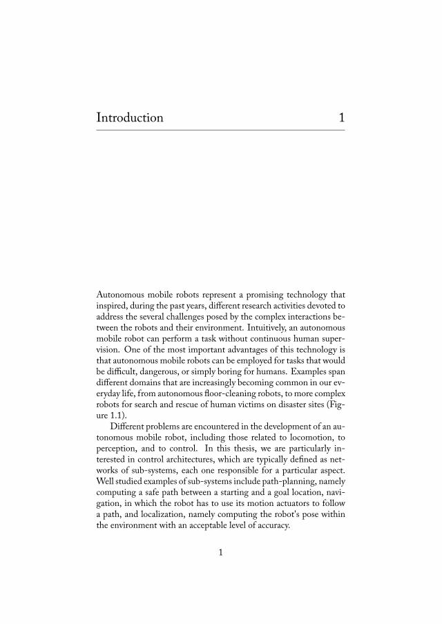
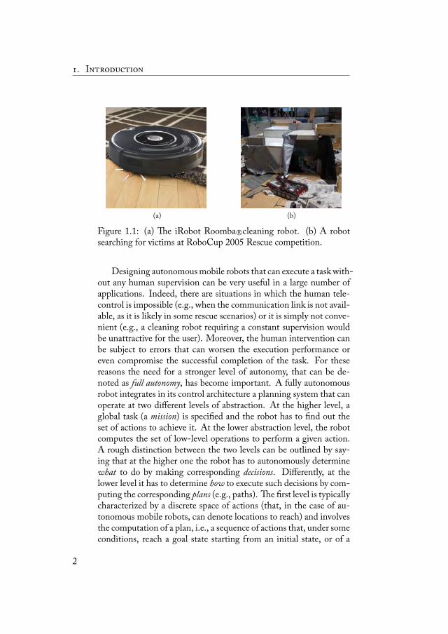
Autonomous mobile robots represent a promising technology thatinspired, during the past years, different research activities devoted toaddress the several challenges posed by the complex interactions be-tween the robots and their environment. Intuitively, an autonomousmobile robot can perform a task without continuous human super-vision. One of the most important advantages of this technology isthat autonomous mobile robots can be employed for tasks that wouldbe difficult, dangerous, or simply boring for humans. Examples spandifferent domains that are increasingly becoming common in our ev-eryday life, from autonomous floor-cleaning robots, to more complexrobots for search and rescue of human victims on disaster sites (Fig-ure 1.1).

Different problems are encountered in the development of an au-tonomous mobile robot, including those related to locomotion, toperception, and to control. In this thesis, we are particularly in-terested in control architectures, which are typically defined as net-works of sub-systems, each one responsible for a particular aspect.Well studied examples of sub-systems include path-planning, namelycomputing a safe path between a starting and a goal location, navi-gation, in which the robot has to use its motion actuators to followa path, and localization, namely computing the robot's pose withinthe environment with an acceptable level of accuracy.

1

. I

(a) (b)

Figure 1.1: (a) e iRobot Roomba R©cleaning robot. (b) A robotsearching for victims at RoboCup 2005 Rescue competition.

Designing autonomousmobile robots that can execute a task with-out any human supervision can be very useful in a large number ofapplications. Indeed, there are situations in which the human tele-control is impossible (e.g., when the communication link is not avail-able, as it is likely in some rescue scenarios) or it is simply not conve-nient (e.g., a cleaning robot requiring a constant supervision wouldbe unattractive for the user). Moreover, the human intervention canbe subject to errors that can worsen the execution performance oreven compromise the successful completion of the task. For thesereasons the need for a stronger level of autonomy, that can be de-noted as full autonomy, has become important. A fully autonomousrobot integrates in its control architecture a planning system that canoperate at two different levels of abstraction. At the higher level, aglobal task (a mission) is specified and the robot has to find out theset of actions to achieve it. At the lower abstraction level, the robotcomputes the set of low-level operations to perform a given action.A rough distinction between the two levels can be outlined by say-ing that at the higher one the robot has to autonomously determinewhat to do by making corresponding decisions. Differently, at thelower level it has to determine how to execute such decisions by com-puting the corresponding plans (e.g., paths). e first level is typicallycharacterized by a discrete space of actions (that, in the case of au-tonomous mobile robots, can denote locations to reach) and involvesthe computation of a plan, i.e., a sequence of actions that, under someconditions, reach a goal state starting from an initial state, or of a

2

1.1. Navigation Strategies for Mobile Robots

strategy (or policy), i.e., a method to decide what action to select in agiven state. e second level typically deals with continuous solutionspaces and requires to compute the low-level operations to executea selected action. Consider, for example, a robot employed for ex-ploring an initially unknown environment to build a map of it. Herean action can prescribe to reach a particular location where the robotcan acquire sensorial data about the environment. In this example,planning at the higher level means to decide a location to reach andplanning at the lower level includes to compute a safe path from therobot's current location to the selected location.

is thesis is about techniques to design strategies, i.e., to equipmobile robots with the ability to make decisions at the higher plan-ning level. An interesting approach to deal with this kind of prob-lems is to exploit techniques from Artificial Intelligence and fromDecision eory [85]. Generally speaking, a mobile robot can bemodeled as an intelligent agent, able to interact both with the en-vironment and with other agents populating it. Decision-theoreticmodels can then be applied to capture the agents' objectives, definehow to measure the goodness of a decision, and compute a strategy.In this dissertation, we focus on the problem an autonomous mobilerobot faces when deciding how to exploit its mobility to completea given task or mission, namely on the problem of deciding where tomove. We refer to this problem as the definition of the mobile robot'snavigation strategy. Our general aim is to contribute to a more formalsystematization of these issues, bringing them under the umbrella ofDecision eory.

1.1 Navigation Strategies for Mobile Robots

To better focus the problem we address, we provide a very generalmodel of the behavior of a fully autonomous mobile robot while ex-ecuting some task:

(a) perform some action in the current location,

(b) decide a location of the environment where to move,

(c) reach the selected location,

(d) return to step (a).

3

. I

Although over-simplified, the above model evidences some interest-ing issues. Step (c) involves low-level planning (e.g., path-planningand localization), while Step (a) relates to actions specific to the taskthat the robot executes at the reached location (e.g., acquire senso-rial data or move some object). e navigation strategy is involvedin Step (c) and we will refer to it according to the following broaddefinition.

A navigation strategy is the set of techniques that allow anautonomous mobile robot to answer the question "where to gonext?", given the knowledge it possesses so far.

For example, in exploration a robot's navigation strategy could be torandomly select next locations or to simply follow a pre-computedtrajectory. In general, the navigation strategy significantly impactson the task execution's performance. erefore, the problem is todefine good navigation strategies, i.e., strategies that allow the robotto perform its taskmaximizing some performancemetric or criterion.

e major challenges related to this problem mainly derive fromtwo issues. e first one is that the definition of a navigation strategystrongly depends on the robot's particular task. Compare, for exam-ple, a robot employed for exploration with another robot that has topatrol an environment. In the first case, the robot should select thelocations to reach such that it can obtain good views of the surround-ings to be integrated in the map. In the second case, the robot has toaccount also for tactical issues such as preventing an intruder to pre-dict its movements and elude it. As this example suggests, differentnavigation strategies should be developed for different tasks.

e second issue is related to the goodness of a navigation strat-egy. Sometimes this concept is intuitively easy to define. For exam-ple, in the case of the surveillance robot one could define the optimalstrategy as the one that minimizes the probability for an intruder tobreak in. However, in other situations the goodness of a navigationstrategy is harder to capture. In the exploration example, differentcriteria contribute to the goodness of a strategy, e.g., the amount ofmapped area, the total traveled distance, the quality of the obtainedmap, the time spent, and many others. In this case, a trade-off be-tween benefits and costs has to be addressed. In general, searchingfor the best strategy according to some metric increases the problem's

4

1.2. Motivations and Objectives

difficulty with respect to the case in which a sub-optimal strategy isemployed.

1.2 Motivations and Objectives

Despite its importance in the development of fully autonomous mo-bile robots, a general satisfactory characterization of the problem ofdefining navigation strategies is still missing. General methods thatcan address wide ranges of applications and that can simplify experi-mental evaluation of navigation strategies have not been exhaustivelystudied. However, as some of the previous examples suggest, navi-gation strategies are a fundamental component in many applicationsfor autonomous mobile robots, and different works in literature dealtwith them. e mainstream approach followed so far seems to adoptad hoc solutions specifically tailored for the particular situation inwhich the robot is deployed, without any attempt to define a moregeneral theoretical framework. For example, in autonomous explo-ration the proposed strategies to determine sensing locations go fromrandom selection or pre-determined trajectories [23] to the so callednext-best-view systems, where a set of locations is evaluated accord-ing to an utility function and the best one is selected [101].

Although many solutions have been proved effective in practice,this trend presents limiting drawbacks. First, it is difficult to comparedifferent strategies with the aim, for example, of selecting the bestone for a given situation. Moreover, modifying a strategy for beingemployed in different contexts or for improving it can require signif-icant efforts. is demand for comparability and flexibility encour-ages the study of more general application-independent frameworkswhere the problem of defining navigation strategies can be cast.

e objective of this dissertation is to contribute along this direc-tion by tackling the problem of defining navigation strategies from amore general perspective. We start from the idea that defining nav-igation strategies is a decision-theoretical problem and that severaladvantages can be obtained when applying techniques coming fromthis field. is idea is not new (e.g., [8, 105]), but we will derivenew original and interesting results within the scope of two appli-cations, namely exploration of unknown environments and surveil-lance. Decision theoretical models are characterized by establishedformal foundations that can enable the development of more general

5

. I

and flexible navigation strategies. For example, some decision theo-retical models allow one to easily combine together different criteriato drive the decision-making process or to model complex scenar-ios characterized by some degree of uncertainty or by the interactionwith other agents. Exploiting general models also simplifies the taskof evaluating and comparing different strategies. From this disser-tation, it emerges that the employment of decision-theoretic tech-niques can, from the one hand, provide a robot with effective nav-igation strategies and, from the other hand, contribute to developmore flexible and comparable navigation strategies.

1.3 ADecision-eoretical Perspective

In order to apply decision-theoretical techniques to develop navi-gation strategies for particular tasks, a classification of the problemunder a decision-theoretical perspective is worth, especially because,as previously discussed, different tasks require different techniques.Navigation strategies can be characterized according to many dimen-sions, here we discuss those that are relevant to the contributions pre-sented in this dissertation, being aware that the list is far from beingdefinitive and complete.

Formally, almost all navigation strategies take as input a state en-closing task-related information about the environment (e.g., in ex-ploration usually it is a map of the currently explored space and thecurrent position of the robot) and provide a set of locations to reachas output. A first distinction can be done between offline and on-line strategies. In the first case, the set of locations to reach is com-puted for every possible input state before the robot actually executesthe task, i.e., before the robot employs the strategy. With an onlinestrategy, instead, the decision is computed during the task execu-tion for the different situations the robot encounters. is distinctioncan also be described with respect to another dimension, namely theamount of available information about the environment. If the envi-ronment (or, more precisely, all the information needed for makingdecisions) is fully known in advance, the robot has a global knowledge.Conversely, if only partial or no environment's information is ini-tially available, the robot has a partial knowledge and should increaseits knowledge to make more informed decisions. e availability ofglobal knowledge results in the possibility of computing the strat-

6

1.3. A Decision-eoretical Perspective

egy offline and, possibly, searching for an optimal solution. On theother hand, a partial knowledge is typically associated with the useof an online navigation strategy where sub-optimal algorithms areemployed.

As an example, consider the two common tasks of coverage andexploration. In coverage, the environment is known in advance andthe robot should cover (possibly, under some constraints) all the freearea. In exploration, the environment is unknown at the beginningand the robot has to ''discover'' it. e first case is characterized bya global knowledge and the optimal strategy, e.g., the shortest route,can be computed offline. e second case is an example of partialknowledge situation for which decisions have to be made online, dueto the impossibility to predict the states that the robot will face. eoptimal strategy cannot be found in general and sub-optimal greedyalgorithms (e.g., next-best-view approaches) must be employed.

e number of decision makers (robots) is another dimension. epresence of multiple agents can pose significant difficulties. Deter-mining a navigation strategy for a team of robots has to deal withthe exponential growth (in the number of robots) of the number ofactions, and usually involves a task-assignment problem [42] wherethe task is a location to be assigned a robot. Multiple robots can co-operate to make a globally optimal decision or can compete to makeindividually optimal decisions.

e presence of multiple agents introduces another dimensionrepresented by the adversarial nature of the setting that is related tothe possible presence of adversaries. An adversary can be defined asa rational agent acting against the robot's objectives, and whose in-teraction has to be considered when computing the navigation strat-egy. Intuitive examples of these last two dimensions can be found inrobotic patrolling. In this application, one or more robots are em-ployed to monitor an environment to prevent intrusions. An adver-sary, i.e., a possible intruder, can be considered by the robots in de-ciding where to move for protecting the environment. In this case, acompetitive interacting scenario emerges and game theoretical tech-niques [74] can be employed to model it and find navigation strate-gies.

7

. I

1.4 Original Contributions

Covering all the possible classes of problems involving navigationstrategies would be non-affordable, therefore we decided to focus ontwo particular applications. e first one is exploration, where therobot is deployed in an initially unknown environment and has toexplore it in order to build a map or to find something. e secondapplication is patrolling, where the environment is known in advanceand the robot has to move around in order to avoid the entrance of apossible intruder. We chose these two applications because of theirpractical importance, confirmed by the significant interest devotedto them by the scientific community. ey have been considered inliterature as separated problems, therefore they exhibit disjoint andtechnically different states of the arts. is is the main reason for pre-senting them separately in two distinct parts of this work. However,despite the differences that these two problems present, the under-lying problem of calculating a navigation strategy is common. Insome sense, we can consider them as instances of the same decision-theoretical problem of answering the question ''where to go next?''.However, this decision-theoretical problem is solved resorting to dif-ferent techniques in the two cases. From a decision-theoretical per-spective, we can identify two different types of challenges related tonavigation strategies in these two domains. We briefly describe themin what follows, listing the original contributions of this work.

Exploration is a very common task in mobile robotics, mainly dueto the large number of applications that require it as pre-requisite,for instance, search and rescue [92] and map building [93]. We con-sidered this problem as characterized by a partial knowledge with anonline strategy in a single agent (non-adversarial) scenario. We studythe employment of a general decision-theoretical technique that con-trasts the several ad hoc solutions presented in literature. More pre-cisely, the contributions of this dissertation in the development ofnavigation strategies for exploration can be summarized as follows(some results have been presented in [16, 58]):

• in the context of next-best-view approaches we provide amulti-objective formulation of the problem of selecting observationlocations;

• we introduce the employment ofMulti-CriteriaDecisionMak-ing (MCDM) [51] as a general and flexible technique to define

8

1.4. Original Contributions

utility functions for the evaluation and selection of candidatelocations;

• we provide an experimental evaluation of MCDM strategies,considering two particular applications: exploration for mapbuilding and for search and rescue.

e second application we address, robotic patrolling, is char-acterized by several open scientific problems, mainly due to the highcomplexity that a patrolling scenario can exhibit. Here the problem ischaracterized by a global knowledge. e environment is fully knownin advance and an offline (optimal) navigation strategy to protect ithas to be computed. e scenario is multi-agent and adversarial,since we explicitly consider the interaction of the robot with an adver-sary (the intruder). We propose novel algorithms to compute optimalpatrolling strategies, that could guarantee the maximum level of pro-tection for a given environment and an optimal fully rational adver-sary. More precisely, the contributions of this dissertation in the de-velopment of navigation strategies for patrolling can be summarizedas follows (some results have been presented in [11, 12, 17, 18]):

• given a game-theoretical patrolling scenario, where two agents(the patrolling robot and the intruder) play against each otherwhile moving in an arbitrary graph-like environment, we pro-pose an algorithm to solve the obtained game determining theoptimal patrolling strategy;

• we provide a set of techniques to reduce the computational ef-fort needed to compute the strategies in order to enable theemployment of our algorithm in realistically large settings;

• we present an experimental evaluation of the efficiency of theproposed technique by testing it on a dataset of patrolling set-tings' instances;

• we showhow the obtained patrolling strategies can be deployedon a realistic robot controller and we conduct tests for evaluat-ing its properties in realistic settings, when some of the theo-retical hypotheses of the model do not hold anymore.

9

. I

1.5 Document Structure

is document is structured in two parts describing our contributionsrelated to exploration and patrolling respectively. Part I encloses thecontributions on autonomous exploration. Chapter 2 surveys therelated works on navigation strategies for exploration of unknownenvironments. Chapter 3 formally introduces Multi-Criteria Deci-sion Making (MCDM) as a general technique to define explorationstrategies by defining flexible global utility functions that, combin-ing different criteria in a general way, can be used to evaluate candi-date observation locations. Chapter 4 and Chapter 5 describe howMCDM can be exploited in two applications where exploration playsa fundamental role, i.e., map building and search and rescue of hu-man victims in a disaster site, respectively.

Part II encloses the contributions on robotic patrolling. Chap-ter 6 reviews the state of the art on patrolling with particular atten-tion on game theoretical approaches. In Chapter 7 we introduce ourgame-theoretical framework to compute optimal patrolling strate-gies and we provide a basic algorithm. In Chapter 8 we describe afirst approach to overcome the computational intractability of non-Markovian strategies in the particular case of deterministic patrollingstrategies. In Chapter 9 we deal with Markovian strategies, describ-ing some game-theoretical techniques to simplify the game and im-prove computational tractability. Chapter 10 discusses experimentalresults with respect to the algorithm's efficiency and to its deploy-ment in a realistic robotic scenario. Chapter 11 concludes this thesisand outlines some directions of future research.

10

Part I

Autonomous Exploration

e first part of this dissertation focuses on autonomous explo-ration. As already anticipated in Chapter 1, this is a task that plays afundamental role in many applicative contexts such as detecting gasor fire sources, cleaning, search and rescue for human victims, andmany others. Here, we will consider a basic version of the prob-lem in which autonomous exploration is characterized by a mobilerobot deployed in an initially unknown environment. e robot isequipped with sensors (e.g., laser range scanners) that allow it to ac-quire spatial data in its surroundings (e.g., the distance of obstacles)within a limited range. It has to move, repeatedly sensing differentportions of the environment, and build a corresponding map. Otherautonomous exploration problems are similarly defined and involve,for example, initially unknown positions of gas or fire sources, of dirt,of human victims, and so on. e problem is characterized by partialknowledge and, in this work, we concentrate on the single robot case.

Navigation strategies (that in this context are also denoted asexploration strategies) allow the robot to determine the locations itshould visit while acquiring information about the environment. How-ever, defining an exploration strategy can involve a large number ofdifferent criteria whose relative importance can vary. For example,one can search for the strategy that minimizes the total time spentin exploration or for the one that minimizes the total distance trav-eled by the robot or for the one that produces the most accurate map.Sometimes the satisfaction of a combination of these criteria can bedesirable also. Partial knowledge prevents from searching the opti-mal strategy. In such situations, if no further information is givena priori, greedy methods, that try to optimize locally (i.e., over sin-gle decisions) instead of globally (i.e., over sequences of decisions)are employed. In this work we consider an iterative next-best-view(NBV) approach, where at each step the robot evaluates a set of can-didate locations and selects the best one according to some objectivefunction. We explicitly remark that the idea that selecting the nextbest sensing location is basically a multi-objective optimization prob-lem, although it has rarely been considered as such in literature. enumber of criteria used to evaluate the goodness of a location canbe large, depending on the particular context in which explorationis involved. erefore, searching for "the best exploration strategy"would be an ill-posed problem and, for this reason, it is not embracedbetween the objectives of this work.

We consider the application of a decision-theoretic technique

called Multi-Criteria Decision Making (MCDM) that allows a de-signer to effectively address the tradeoff among the different criteriaemployed in the evaluation of a candidate location. In particular, westudy and experimentally validate the application of MCDM tech-niques to the definition of multi-objective utility functions to be usedfor evaluating candidate locations in exploration.

Approaches for Exploration Strategies 2

Exploration strategies are used to move autonomous robots aroundinitially unknown environments in order to incrementally ''discover''their features. For example, inmap building the ''discovered'' featuresare the obstacles and the free space, while in search and rescue canbe the locations of the victims.

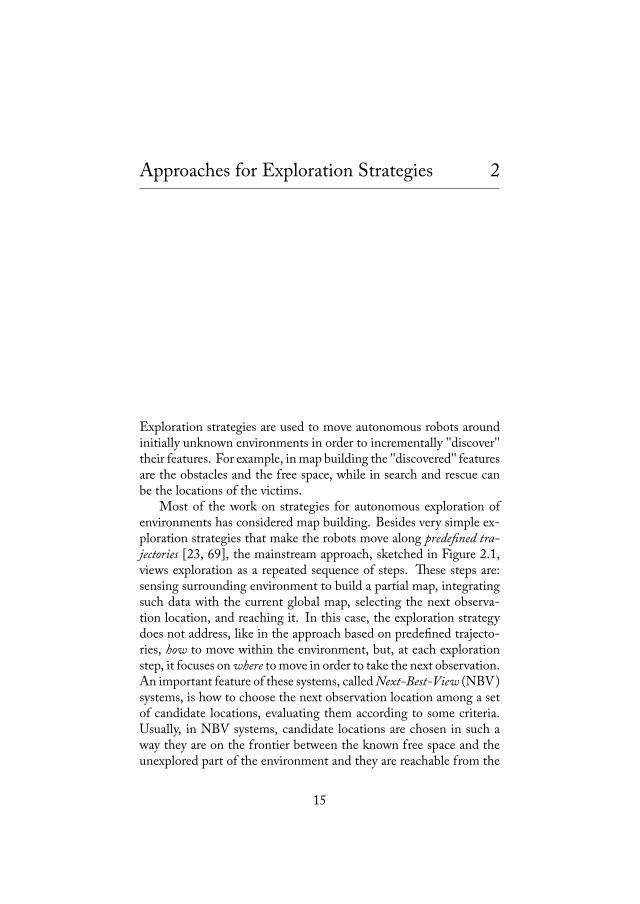
Most of the work on strategies for autonomous exploration ofenvironments has considered map building. Besides very simple ex-ploration strategies that make the robots move along predefined tra-jectories [23, 69], the mainstream approach, sketched in Figure 2.1,views exploration as a repeated sequence of steps. ese steps are:sensing surrounding environment to build a partial map, integratingsuch data with the current global map, selecting the next observa-tion location, and reaching it. In this case, the exploration strategydoes not address, like in the approach based on predefined trajecto-ries, how to move within the environment, but, at each explorationstep, it focuses onwhere tomove in order to take the next observation.An important feature of these systems, calledNext-Best-View (NBV)systems, is how to choose the next observation location among a setof candidate locations, evaluating them according to some criteria.Usually, in NBV systems, candidate locations are chosen in such away they are on the frontier between the known free space and theunexplored part of the environment and they are reachable from the

15

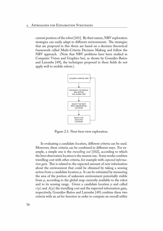
. A E S

current position of the robot [101]. By their nature, NBV explorationstrategies can easily adapt to different environments. e strategiesthat are proposed in this thesis are based on a decision theoreticalframework called Multi-Criteria Decision Making and follow theNBV approach. (Note that NBV problems have been studied inComputer Vision and Graphics but, as shown by Gonzales-Banosand Latombe [49], the techniques proposed in these fields do notapply well to mobile robots.)

Figure 2.1: Next-best-view exploration.

In evaluating a candidate location, different criteria can be used.Moreover, these criteria can be combined in different ways. For ex-ample, a simple one is the travelling cost [102], according to whichthe best observation location is the nearest one. Someworks combinetravelling cost with other criteria, for example with expected informa-tion gain. is is related to the expected amount of new informationabout the environment that could be obtained by taking a sensingaction from a candidate location p. It can be estimated by measuringthe area of the portion of unknown environment potentially visiblefrom p, according to the global map currently available to the robotand to its sensing range. Given a candidate location p and calledc(p) and A(p) the travelling cost and the expected information gain,respectively, Gonzales-Banos and Latombe [49] combine these twocriteria with an ad hoc function in order to compute an overall utility

16

(λ weighs the travelling cost and the information gain):

u(p) = A(p)e−λc(p) (2.1)

Similar criteria are considered by Stachniss and Burgard [90], wherethe cost of reaching a candidate location p is linearly combined withits benefits. Measuring the cost as the distance d(p) from the currentrobot's location and the benefit as an estimate of the new informationA(p) acquirable from p, the global utility of p is computed as:

u(p) = A(p)− βd(p) (2.2)

where β balances the relative weight of benefits versus cost and isusually chosen in the interval [0.01, 50] (authors show that choosingwithin this interval does not causes significant variations in the explo-ration performance). Other examples include the work of Amigoniet al. [9], in which a technique based on relative entropy is used, andof Tovar et al. [94], where several criteria are employed to evaluate acandidate location: travelling cost, uncertainty in landmark recogni-tion, number of visible features, length of visible free edges, rotationand number of stops needed to follow the path to the location. eyare combined in a multiplicative function (in order to guarantee thatlocations with a good global utility satisfy well all the criteria) to ob-tain a global utility value.

e above strategies aggregate different criteria in utility func-tions that are defined ad hoc and are strongly dependent on the cri-teria they combine. Amigoni and Gallo [8] dealt with this prob-lem and proposed a more theoretically-grounded approach based onmulti-objective optimization, in which the best candidate location isselected on the Pareto frontier. Besides distance and expected in-formation gain, also overlap is taken into account. is criterion isrelated to the amount of old information that will be acquired againfrom a candidate location. Maximizing the overlap can improve theperformance of self-localization of the robot.

Some solutions have been also proposed for multirobot scenarioswhere map building is performed by a team of robots. In this case,besides the problem of evaluating candidate locations, also a robot-location assignment problem has to be addressed. A seminal workhas been proposed by Burgard et al. [24] where each robot evaluatesa candidate location by means of a weighted aggregation functionwhich combines two criteria: the travelling cost and a general mea-sure of goodness, initially equal for all candidates, that decreases once

17

. A E S

a location is assigned to a robot. With this method robots tend tospread over the environment, avoiding to make perceptions in prox-imity of other robots. Other examples of combinations of criteriainclude the work of Zlot et al. [105], where the robot-location as-signment problem is addressed by exploiting a coordination paradigmbased on a market economy approach, and of Franchi et al. [38]where a cooperative exploration strategy based on Sensor-based Ran-dom Trees (representing roadmaps of the environment) is proposedas an extension of previous works [73] for the single robot case. Fi-nally, Haumann et al. [55] consider location selection and path plan-ning as a joint task in an objective function combining distance, ori-entation costs, and estimated information gain to select a collisionfree path.

Compared with exploration strategies for map building, relativelyfewworks proposed exploration strategies for autonomous search andrescue. A work that explicitly addressed this problem has been pro-posed by Visser and Slame [98]. Authors propose to combine thedistance, the expected information gain, and the probability of a suc-cessful communication from a candidate location in a fractional non-linear function. is strategy has been employed, with good results,in different RoboCup Rescue Virtual Robots Competitions. An-other example the work of Calisi et al. [25], where a formalism basedon Petri nets is employed for the definition of an exploration strat-egy that exploits a priori information about the victims' distribution(e.g., if they are uniformly spread or concentrated in few clusters) toimprove the search.

A number of works can also be found in the theoretical com-puter science literature, where the problem of exploring a polygonalenvironment with a mobile robot is addressed with a computationalgeometry approach (see [43] for a survey of algorithms). For exam-ple Hoffmann et al. [56] propose an on-line algorithm to explorean unknown simple polygon that outperforms the offline computedshortest watchman route. Icking et al. [60] dealt with grid-based en-vironments and propose an algorithm to cover all the free cells withthe minimum number of multiple visits to a same cell. A last signif-icant example has been proposed by Fekete and Schmidt [36] wherepolygons exploration is performed with a mobile robot characterizedby a discrete perception, i.e, the impossibility of scanning the envi-ronment continuously while in motion. e important ideal assump-tions made in these works make them not directly applicable to real

18

robotic scenarios.According to the broad objectives of this thesis, in the following

chapters we propose the adoption of a decision theoretical frameworkcalled Multi-Criteria Decision Making (MCDM) for the definitionof exploration strategies in two popular applicative contexts in whichautonomous exploration plays a fundamental role: map building andsearch and rescue. MCDM is a more theoretically-grounded andflexible way to combine criteria that should be contrasted with ad hoccompositions (like weighted mean of [90], the multiplicative func-tion of [94], and the other works listed above). is technique dealswith problems in which a decisionmaker has to choose among a set ofalternatives and its preferences depend on different, and sometimesconflicting, criteria. It is employed in several applicative domainssuch as Economy, Ecology, and Computer Science [51, 89]. eChoquet fuzzy integral [52] is used in MCDM to combine differ-ent criteria in a global utility function whose main advantage is thepossibility to account for the relations between criteria [50, 51]. eresults presented in the following chapters have been discussed, in avery preliminary form, in [16].

19

A Decision eoretical Framework forExploration Strategies 3

In this chapter, we formally introduce Multi-Criteria Decision Mak-ing (MCDM) as a genenral and flexible tool for defining explorationstrategies.

3.1 Evaluating Observation Locations

When designing an effective NBV exploration strategy, the mainchallenge is to achieve a good long-term performance by means ofshort-term decisions that are made on the basis of partial knowledge.As discussed in the previous chapter, choosing observation locationscan involve several evaluation criteria, ranging from travelling dis-tance to estimates of the information gain that can be obtained ina particular location. erefore, the problem of evaluating candi-date observation locations can be more properly modeled as a multi-objective optimization problem where objectives are encoded in thecriteria used for evaluating locations. emajority of techniques pro-posed in literature do not follow this approach and combine a numberof criteria into a global utility function, whose maximization leads tothe selection of the best observation location. However, often suchmethods strongly depend on the number of criteria they combine

21

. A D T F

and the way they are computed. ey can be difficult to extend, forexample introducing new criteria, and can be hardly exploited in ap-plicative contexts different from the one they have been tailored for.

Another significant aspect is a criterion can be computed in mul-tiple ways. For instance, the information gain estimate conceptu-ally represents a single criterion but it can be computed, for exam-ple, by estimating the new area or by measuring the length of thevisible frontier between mapped and unknown space. In the sameway, some criteria can be substantially different but intrinsically ac-count for very similar selection principles (e.g., the distance of a can-didate location and the time needed to reach it). From a general anddecision-theoretical perspective, this aspect comes from the fact thatcriteria, in general, are not independent one from each other. Howto consider possible dependencies when combining them in an util-ity function can be a very important and sometimes hard issue to beaddressed.

In what follows, we describe a decision-theoretical technique thatpresents interesting features with respect to what discussed above.is technique is called Multi-Criteria Decision Making (MCDM)and allows to find Pareto optimal candidates, to easily extend theevaluation function with new criteria, and to account for dependen-cies between criteria. e robot is modeled as a generic decisionmaker and a flexible aggregation function is exploited for combin-ing different criteria.

3.2 UsingMCDM to Combine Utilities

e formulation of the problem to be addressed by a NBV strategy isstraightforward: given a set of alternatives C, choose the ''best'' oneamong them. Despite the simplicity of its formulation, the definitionof ''best'' has not yet found a theoretically sound solution. Formally,we will denote as criteria the features for evaluating candidate loca-tions and we will denote by ui(p) the utility of a candidate p ∈ Cwith respect to criterion i. Utility is a measure of how good a candi-date is with respect to the considered criterion. Without any loss ofgenerality, we will assume that ui(p) ∈ [0, 1] and that the larger theutility, the better a candidate. In this way, we have a common scale ofevaluation for each criterion. If we assume to have n criteria denotedby the set N = {1, 2, . . . , n}, a candidate p can be associated to a

22

3.2. Using MCDM to Combine Utilities

vector of n elements, namely its utilities, (u1(p), u2(p), . . . , un(p)).Hence, the Pareto frontier ofC can be determined as the largest sub-setP ⊆ C such that for every p ∈ P there is not any candidate q ∈ Cwith ui(q) > ui(p) for all i ∈ N .

Informally, providing amethod to select a candidate on the Paretofrontier amounts to define the meaning of ''best''. e proposedMCDM approach solves this problem by providing a general wayto define a global utility function, according to which a candidate onthe Pareto frontier is selected. Global utility can be simply definedas a (non decreasing) aggregation function which combines all theutilities of a candidate p to obtain an overall evaluation of p. We willdenote global utility as u : [0, 1]n → [0, 1]. Examples of well-knownaggregation functions are the arithmetic or weighted mean. Givenu, we can determine the Pareto optimal candidate that maximizes it,thus selecting the ''best'' candidate.

To better motivate the MCDM approach, let us introduce anexample. Suppose to evaluate a candidate location p considering thefollowing three criteria (for presentation purposes, here we providea concise description of criteria that will be fully detailed in the nextchapters):

• the travelling cost c as the distance from the robot's currentposition to p;

• the area-based information gain estimate iArea as the area ofunknown space potentially visible by the robot at p;

• the segments-based information gain estimate iSeg as the lengthof the frontier between mapped and unknown space the robotcan sense at p;

ese criteria define the setN = {c, iArea, iSeg}. e simplest wayto compute a global utility starting from the single utilities is to use aweighted average as aggregation function, as in [24]. For example, letus suppose that we want to give slight more importance to acquiringnew information than to saving energy in movements. We can setthe following weights, representing the relative importance of thecriteria:

23

. A D T F

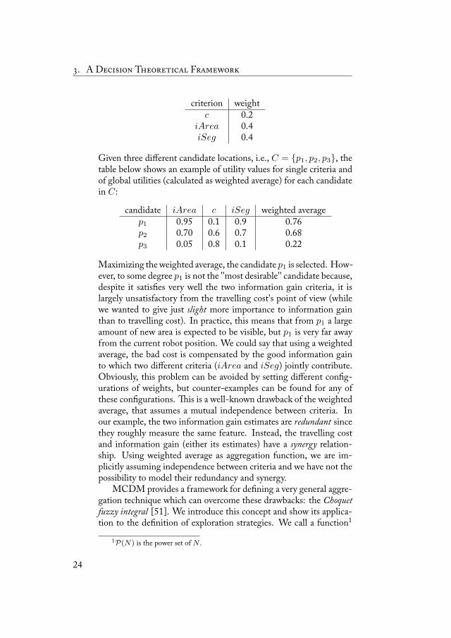
criterion weightc 0.2

iArea 0.4iSeg 0.4

Given three different candidate locations, i.e., C = {p1, p2, p3}, thetable below shows an example of utility values for single criteria andof global utilities (calculated as weighted average) for each candidatein C:

candidate iArea c iSeg weighted averagep1 0.95 0.1 0.9 0.76p2 0.70 0.6 0.7 0.68p3 0.05 0.8 0.1 0.22

Maximizing theweighted average, the candidate p1 is selected. How-ever, to some degree p1 is not the ''most desirable'' candidate because,despite it satisfies very well the two information gain criteria, it islargely unsatisfactory from the travelling cost's point of view (whilewe wanted to give just slight more importance to information gainthan to travelling cost). In practice, this means that from p1 a largeamount of new area is expected to be visible, but p1 is very far awayfrom the current robot position. We could say that using a weightedaverage, the bad cost is compensated by the good information gainto which two different criteria (iArea and iSeg) jointly contribute.Obviously, this problem can be avoided by setting different config-urations of weights, but counter-examples can be found for any ofthese configurations. is is a well-known drawback of the weightedaverage, that assumes a mutual independence between criteria. Inour example, the two information gain estimates are redundant sincethey roughly measure the same feature. Instead, the travelling costand information gain (either its estimates) have a synergy relation-ship. Using weighted average as aggregation function, we are im-plicitly assuming independence between criteria and we have not thepossibility to model their redundancy and synergy.

MCDM provides a framework for defining a very general aggre-gation technique which can overcome these drawbacks: the Choquetfuzzy integral [51]. We introduce this concept and show its applica-tion to the definition of exploration strategies. We call a function1

1P(N) is the power set of N .

24

3.2. Using MCDM to Combine Utilities

µ : P(N) → [0, 1] a fuzzy measure on the set of criteria N when itsatisfies the following properties:

1. µ(∅) = 0, µ(N) = 1,

2. if A ⊂ B ⊂ N then µ(A) ≤ µ(B).

Given A ∈ P(N), µ(A) represents the weight of the set of criteriaA. In this way, weights are associated not only to single criteria,but also to their combinations. Global utility u(p) for a location p iscomputed by means of the Choquet integral with respect to the fuzzymeasure µ:

u(p) =n∑

j=1

(u(j)(p)− u(j−1)(p))µ(A(j)), (3.1)

where (j) indicates the indices after a permutation that changed theirorder to have, for a given p, u(1)(p) ≤ . . . ≤ u(n)(p) ≤ 1 (it is sup-posed that u(0)(p) = 0) and

A(j) = {i ∈ N |u(j)(p) ≤ ui(p) ≤ u(n)(p)}.

Different aggregation functions can be defined by changing the def-inition of µ. For example, weighted average is a particular case ofthe Choquet integral when µ is additive (i.e., µ(A ∪ B) = µ(A) +µ(B)). Most importantly, through µ it is possible to model two dif-ferent types of dependency relationships between criteria. e firstone models the situation in which, when combining criteria into theaggregation function, their joint contribution to the global utilityshould be less than the sum of their individual ones. In this case,a redundancy relation holds between criteria. e more redundanttwo criteria are, the more strongly good utilities for one will counter-balance bad utilities for the other. A symmetric situation occurs whentwo or more criteria are very different and, in general, can be hardlyoptimized together. In this case, a synergy relation holds betweenthem, and their joint contribution should be considered larger thanthe sum of the individual ones. When two criteria are synergic, goodutilities for both are very difficult to achieve in a single candidate andcandidates that satisfy both criteria reasonably well should be pre-ferred to candidates that satisfy them in an unbalanced way. Moreformally, given two criteria c1 and c2 and their weights µ(c1) andµ(c2):

25

. A D T F

• if µ({c1, c2}) < µ(c1) + µ(c2) the two criteria are said to beredundant,

• if µ({c1, c2}) > µ(c1) + µ(c2) the two criteria are said to besynergic.

e same principle holds for sets of more than two criteria. Return-ing to the above example, we can keep the same weights for the singlecriteria:

µ(iArea) = 0.4µ(c) = 0.2µ(iSeg) = 0.4

but we can now model redundancy between iArea and iSeg andsynergy between them and travelling cost c, for instance setting thefollowing values:

µ({iArea, c}) = 0.8µ({iArea, iSeg}) = 0.5µ({c, iSeg}) = 0.8

Applying the Choquet integral with the above definition of µ, wehave the following utility values:

candidate iArea c iSeg Choquet integralp1 0.95 0.1 0.9 0.52p2 0.70 0.6 0.7 0.65p3 0.05 0.8 0.1 0.23

What has been obtained is a sort of ''distorted'' weighted average,which takes into account dependency between criteria. Now the se-lected candidate is p2, which is the candidate that is expected to pro-vide visibility over large areas of unknown environment but that isreasonably close to the current robot position.

In the following chapters, we exploit MCDM to develop ex-ploration strategies, namely to define utility functions that drive therobot's selection of the next observation location. To show its prop-erties, we developed MCDM-based exploration strategies in differ-ent applications involving the exploration of unknown environments.In each setting, we define groups of criteria and we assign a corre-sponding set of weights. is last step can be particularly tricky. In-deed, in this phase, the designer considers the particular applicative

26

3.2. Using MCDM to Combine Utilities

domain and defines a trade-off in specifying the importance of sin-gle criteria and their groups. We remark the idea that searching forthe ''best'' set of weights is a meaningless problem in the context ofMCDM. MCDM is not a method to determine the best explorationstrategy, but provides a flexible tool to combine criteria. erefore,we assigned weights manually, considering the particular applicativescenario. is manual method does not scale well with the num-ber n of criteria since 2n − 2 weights have to be assigned. However,semi-automated techniques can compute weights for large sets of cri-teria. As described in [51], the designer can specify constraints overweights and feasible sets of values can be automatically computed.

e first setting (Chapter 4) concerns exploration for map build-ing, i.e., a setting in which a robot's task is to build a map of theenvironment. e second setting (Chapter 5) deals with a searchand rescue domain [15], where exploration drives the robot to searchfor human victims in a disaster environment. MCDM-based strate-gies are experimentally evaluated and compared with other strategiesto measure their performance and to asses if MCDM can be a validalternative to the methods proposed in literature.

27

Exploration Strategies for Map Building 4

In this chapter, we apply MCDM to the definition of explorationstrategies for map building where the objective is to efficiently pro-duce a map of the environment. We present results obtained in twodifferent experimental settings where the mapping task is performedby a single robot. To better focus on the performance of navigationstrategies, we conducted tests in simulation, using realistic and pop-ular robotic simulators.

4.1 Building Geometrical Maps with DiscretePerceptions

In this setting we consider a simple scenario where the robot main-tains a geometrical map, localization and movement errors of therobot are not considered, and the perception is discrete, i.e., the robotacquires spatial data only at the selected observation locations and notwhen it moves.

4.1.1 Exprimental SettingWe assume to have a mobile robot equipped with a laser range scan-ner sensor able to acquire 360◦ range data within a range r. Explo-ration is performed as a sequence of discrete perceptions, namely the

29

. E S M B

robot senses the surroundings only at the selected observation loca-tion p and not along the path that connects its current position top.

e map is represented with 2D line segments, organized in twolists. e obstacle list contains the line segments representing theboundaries of the obstacles detected in the environment. e freeedge list stores the line segments representing the frontiers betweenknown and unknown space. Line segments are obtained from datareturned by the sensor in the following way. At each observation lo-cation, a 360◦ scan of the environment, with a resolution of 0.5◦,is performed by the laser range scanner. A set of 720 points is ob-tained, expressed in a polar coordinate system centered in the sensorposition. A point is thus represented by an angle θ and a distance ρ.Points are then classified with respect to ρ as free edge points (whenρ = r) or as obstacle points (when ρ < r). Line segments are theparts of the polylines obtained by joining points of those sets. Eachobservation produces a partial map m, which is integrated in a globalmap M , in order to incrementally build a complete representation ofthe environment. In a partial map m obtained after an observation,there are line segments representing obstacles and line segments rep-resenting free edges1. e global map M is updated by aligning mto M (according to the position of the robot, that is assumed to beknown exactly) and by fusing their line segments. Obstacle line seg-ments of m are added to the obstacle list of M and, similarly, freeedges ofm are inserted in the free edge list ofM . Moreover, old freeedges ofM which, after the observation, belong to the explored area,are deleted from the corresponding list.

Following the frontier-based approach [8, 101], we generate theset of candidate locations by considering the middle points of the linesegments in the free edge list. Hence, there are as many candidatelocations as line segments in the free edge list.

Given a candidate location p, we consider up to four criteria forits evaluation. e travelling cost c(p) is computed as the length ofthe path connecting the current position of the robot with p. Forpath-planning purposes, a reachability tree is maintained during theexploration, similarly to [82]. Leaves are associated to current candi-date locations while internal nodes are previously visited observation

1We consider as free edges also line segments between two obstacle points (θ, ρ1)and (θ + 0.5◦, ρ2) such that |ρ1 − ρ2| is larger than a threshold.

30

4.1. Building Geometrical Maps with Discrete Perceptions

(a) iArea(p) (b) iSeg(p)

(c) o(p)

Figure 4.1: Information gain estimates and overlap for a candidatelocation p.

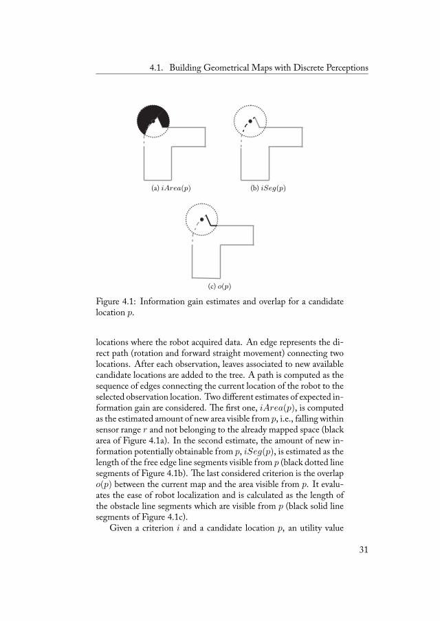
locations where the robot acquired data. An edge represents the di-rect path (rotation and forward straight movement) connecting twolocations. After each observation, leaves associated to new availablecandidate locations are added to the tree. A path is computed as thesequence of edges connecting the current location of the robot to theselected observation location. Two different estimates of expected in-formation gain are considered. e first one, iArea(p), is computedas the estimated amount of new area visible from p, i.e., falling withinsensor range r and not belonging to the already mapped space (blackarea of Figure 4.1a). In the second estimate, the amount of new in-formation potentially obtainable from p, iSeg(p), is estimated as thelength of the free edge line segments visible from p (black dotted linesegments of Figure 4.1b). e last considered criterion is the overlapo(p) between the current map and the area visible from p. It evalu-ates the ease of robot localization and is calculated as the length ofthe obstacle line segments which are visible from p (black solid linesegments of Figure 4.1c).

Given a criterion i and a candidate location p, an utility value

31

. E S M B

ui(p) in the [0, 1] interval is computed in order to evaluate on a com-mon scale p's goodness according to every criterion. e utility isdefined by normalization over all the candidates in the current ex-ploration step. For example, considering the travelling cost c(p) andcalled C the set of (current) candidate locations, the utility uc(p)(with p ∈ C) is computed with the following linear mapping func-tion:

uc(p) = 1− (c(p)− minq∈C c(q))

(maxq∈C c(q)− minq∈C c(q))

e same normalization technique is employed for all other criteriaused in our experiments, with the idea that the larger the utility valuethe better the satisfaction of the criterion. e use of relative nor-malization is justified by the independence between different robot'schoices at different steps. Indeed, due to the greedy nature of theNBV approach (Figure 2.1), the result of the robot's decision at anystep depends only on C and not on previous decisions and previoussets of candidate locations.

In order to compare the MCDM approach with other proposedtechniques, in this setting we considered two exploration strategiestaken from literature. e first one is a strategy based on the weightedaverage, as in [24], where the criteria c, iArea, and iSeg are com-bined together with the weights reported in the second and thirdcolumns of Table 4.1. We will refer to this strategy as the WA strat-egy. e second one is the strategy proposed in [49] where c andiArea are combined using (2.1) (this strategy was tested imposingλ = 0.2 1

m as suggested in the original paper, we denote it as Latombestrategy).

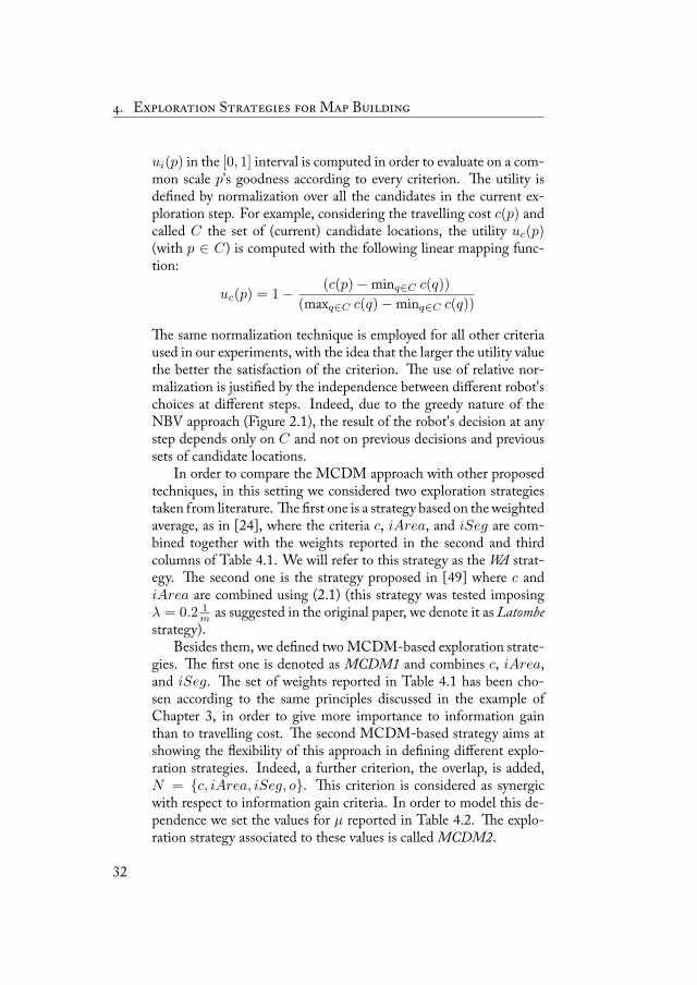
Besides them, we defined two MCDM-based exploration strate-gies. e first one is denoted as MCDM1 and combines c, iArea,and iSeg. e set of weights reported in Table 4.1 has been cho-sen according to the same principles discussed in the example ofChapter 3, in order to give more importance to information gainthan to travelling cost. e second MCDM-based strategy aims atshowing the flexibility of this approach in defining different explo-ration strategies. Indeed, a further criterion, the overlap, is added,N = {c, iArea, iSeg, o}. is criterion is considered as synergicwith respect to information gain criteria. In order to model this de-pendence we set the values for µ reported in Table 4.2. e explo-ration strategy associated to these values is called MCDM2.

32

4.1. Building Geometrical Maps with Discrete Perceptions

MCDM1 criteria µ() criteria µ()

c 0.2 {c, iArea} 0.9iArea 0.4 {c, iSeg} 0.9iSeg 0.4 {iArea, iSeg} 0.6

Table 4.1: Definition of µ for the MCDM1 strategy.

MCDM2

criteria µ() criteria µ()c 0.3 {iArea, iSeg} 0.2

iArea 0.2 {iArea, o} 0.5iSeg 0.2 {iSeg, o} 0.5o 0.2 {c, iArea, iSeg} 0.8

{c, iArea} 0.8 {c, iArea, o} 0.9{c, iSeg} 0.8 {c, iSeg, o} 0.9{c, o} 0.5 {iArea, iSeg, o} 0.45

Table 4.2: Definition of µ for the MCDM2 strategy.

4.1.2 Experimental Evaluation

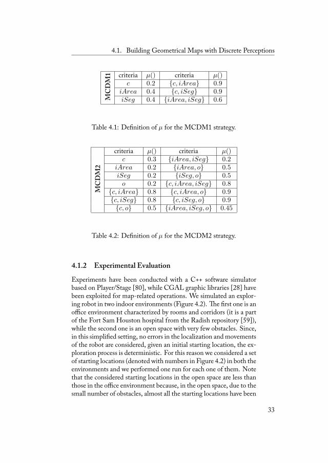
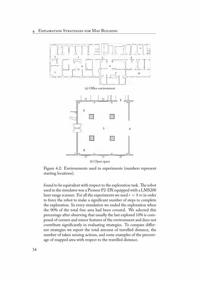
Experiments have been conducted with a C++ software simulatorbased on Player/Stage [80], while CGAL graphic libraries [28] havebeen exploited for map-related operations. We simulated an explor-ing robot in two indoor environments (Figure 4.2). e first one is anoffice environment characterized by rooms and corridors (it is a partof the Fort Sam Houston hospital from the Radish repository [59]),while the second one is an open space with very few obstacles. Since,in this simplified setting, no errors in the localization and movementsof the robot are considered, given an initial starting location, the ex-ploration process is deterministic. For this reason we considered a setof starting locations (denoted with numbers in Figure 4.2) in both theenvironments and we performed one run for each one of them. Notethat the considered starting locations in the open space are less thanthose in the office environment because, in the open space, due to thesmall number of obstacles, almost all the starting locations have been

33

. E S M B

(a) Office environment

(b) Open space

Figure 4.2: Environments used in experiments (numbers representstarting locations).

found to be equivalent with respect to the exploration task. e robotused in the simulator was a Pioneer P2-DX equipped with a LMS200laser range scanner. For all the experiments we used r = 8m in orderto force the robot to make a significant number of steps to completethe exploration. In every simulation we ended the exploration whenthe 90% of the total free area had been covered. We selected thispercentage after observing that usually the last explored 10% is com-posed of corners and minor features of the environment and does notcontribute significantly in evaluating strategies. To compare differ-ent strategies we report the total amount of travelled distance, thenumber of taken sensing actions, and some examples of the percent-age of mapped area with respect to the travelled distance.

34

4.1. Building Geometrical Maps with Discrete Perceptions

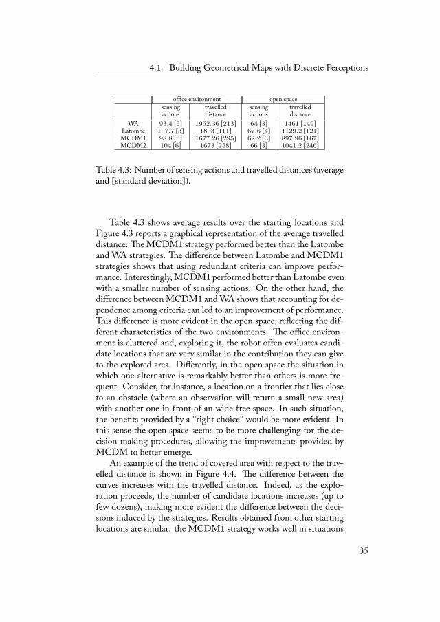
office environment open spacesensing travelled sensing travelledactions distance actions distance

WA 93.4 [5] 1952.36 [213] 64 [3] 1461 [149]Latombe 107.7 [3] 1803 [111] 67.6 [4] 1129.2 [121]MCDM1 98.8 [3] 1677.26 [295] 62.2 [3] 897.96 [167]MCDM2 104 [6] 1673 [258] 66 [3] 1041.2 [246]

Table 4.3: Number of sensing actions and travelled distances (averageand [standard deviation]).

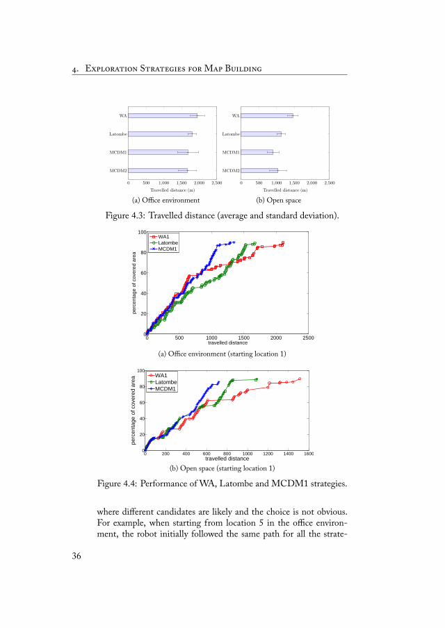
Table 4.3 shows average results over the starting locations andFigure 4.3 reports a graphical representation of the average travelleddistance. e MCDM1 strategy performed better than the Latombeand WA strategies. e difference between Latombe and MCDM1strategies shows that using redundant criteria can improve perfor-mance. Interestingly,MCDM1performed better thanLatombe evenwith a smaller number of sensing actions. On the other hand, thedifference between MCDM1 and WA shows that accounting for de-pendence among criteria can led to an improvement of performance.is difference is more evident in the open space, reflecting the dif-ferent characteristics of the two environments. e office environ-ment is cluttered and, exploring it, the robot often evaluates candi-date locations that are very similar in the contribution they can giveto the explored area. Differently, in the open space the situation inwhich one alternative is remarkably better than others is more fre-quent. Consider, for instance, a location on a frontier that lies closeto an obstacle (where an observation will return a small new area)with another one in front of an wide free space. In such situation,the benefits provided by a ''right choice'' would be more evident. Inthis sense the open space seems to be more challenging for the de-cision making procedures, allowing the improvements provided byMCDM to better emerge.

An example of the trend of covered area with respect to the trav-elled distance is shown in Figure 4.4. e difference between thecurves increases with the travelled distance. Indeed, as the explo-ration proceeds, the number of candidate locations increases (up tofew dozens), making more evident the difference between the deci-sions induced by the strategies. Results obtained from other startinglocations are similar: the MCDM1 strategy works well in situations

35

. E S M B

0 500 1,000 1,500 2,000 2,500

MCDM2

MCDM1

Latombe

WA

Travelled distance (m)

(a) Office environment

0 500 1,000 1,500 2,000 2,500

MCDM2

MCDM1

Latombe

WA

Travelled distance (m)

(b) Open space

Figure 4.3: Travelled distance (average and standard deviation).

0 500 1000 1500 2000 25000

20

40

60

80

100

travelled distance

perc

enta

ge o

f cov

ered

are

a

WA1LatombeMCDM1

(a) Office environment (starting location 1)

0 200 400 600 800 1000 1200 1400 16000

20

40

60

80

100

travelled distance

perc

enta

ge o

f cov

ered

are

a

WA1LatombeMCDM1

(b) Open space (starting location 1)

Figure 4.4: Performance of WA, Latombe and MCDM1 strategies.

where different candidates are likely and the choice is not obvious.For example, when starting from location 5 in the office environ-ment, the robot initially followed the same path for all the strate-

36

4.2. Building Grid-Based Maps with Continuous Perceptions

gies (i.e., it went outside the left bottom room). However, once therobot reached the main horizontal corridor, paths, and consequentlyperformances, started to differ according to the strategies, and theMCDM1 strategy drove the robot in the right bottom direction re-sulting in a more efficient exploration than other strategies that drovethe robot up.

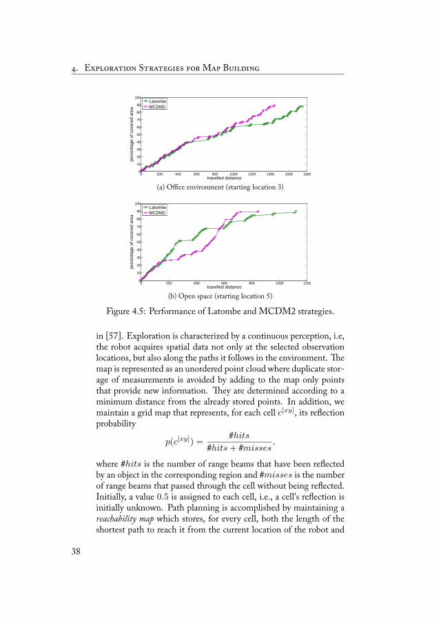
As reported in the last row of Table 4.3, the MCDM2 strategyshows a worsening of the performance with respect to MCDM1. In-deed, this strategy is sometimes penalized in terms of distance trav-elled by the overlap criterion. is can be explained by consideringthat it is often the case when MCDM2 brings the robot towards lo-cations not close to its current position or with limited informationgain in order to guarantee a good level of overlap (see also [7] for adiscussion of this behavior). As expected, this is more evident in theopen space environment where, due to the presence of few obstacles,the satisfaction of the overlap criterion is more difficult. Despite thepenalization introduced by the overlap criterion, we observed situa-tions, like the one depicted in Figure 4.5, in which MCDM2 per-formed better than the Latombe strategy. e advantages of usingthe overlap criterion could be measured in terms of better robot self-localization. However, a quantitative evaluation of these advantagesheavily depends on the localization method used by the robot that, inthis experimental setting, has not been employed (being localizationerror-free).

4.2 Building Grid-BasedMaps with ContinuousPerceptions

We now introduce our second experimental setting in which we eval-uated the MCDM approach. Compared to the previous one, this isa more realistic setting since movement and localization errors areexplicitly considered and the map has a grid-based representation.Moreover, the robot performs a continuous perception, acquiringdata also while moving.

4.2.1 Experimental Setting

Robot localization and mapping are performed by incrementally reg-istering raw 2D laser range scans following the approach proposed

37

. E S M B

0 200 400 600 800 1000 1200 1400 1600 18000

10

20

30

40

50

60

70

80

90

100

travelled distance

perc

enta

ge o

f cov

ered

are

a

LatombeMCDM2

(a) Office environment (starting location 3)

0 200 400 600 800 1000 12000

10

20

30

40

50

60

70

80

90

100

travelled distance

perc

enta

ge o

f cov

ered

are

a

LatombeMCDM2

(b) Open space (starting location 5)

Figure 4.5: Performance of Latombe and MCDM2 strategies.

in [57]. Exploration is characterized by a continuous perception, i.e,the robot acquires spatial data not only at the selected observationlocations, but also along the paths it follows in the environment. emap is represented as an unordered point cloud where duplicate stor-age of measurements is avoided by adding to the map only pointsthat provide new information. ey are determined according to aminimum distance from the already stored points. In addition, wemaintain a grid map that represents, for each cell c[xy], its reflectionprobability

p(c[xy]) =#hits

#hits+ #misses,

where #hits is the number of range beams that have been reflectedby an object in the corresponding region and #misses is the numberof range beams that passed through the cell without being reflected.Initially, a value 0.5 is assigned to each cell, i.e., a cell's reflection isinitially unknown. Path planning is accomplished by maintaining areachability map which stores, for every cell, both the length of theshortest path to reach it from the current location of the robot and

38

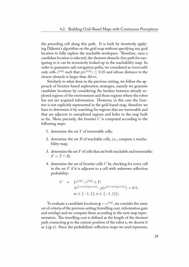
4.2. Building Grid-Based Maps with Continuous Perceptions

the preceding cell along this path. It is built by iteratively apply-ing Dijkstra's algorithm on the grid map without specifying any goallocation to fully explore the reachable workspace. erefore, once acandidate location is selected, the shortest obstacle-free path for nav-igating to it can be recursively looked up in the reachability map. Inorder to guarantee safe navigation paths, we considered as traversableonly cells c[xy] such that p(c[xy]) ≤ 0.25 and whose distance to theclosest obstacle is larger than 30cm.

Similarly to what done in the previous setting, we follow the ap-proach of frontier-based exploration strategies, namely we generatecandidate locations by considering the borders between already ex-plored regions of the environment and those regions where the robothas not yet acquired information. However, in this case the fron-tier is not explicitly represented in the grid-based map, therefore wehave to determine it by searching for regions that are traversable andthat are adjacent to unexplored regions and holes in the map builtso far. More precisely, the frontier C is computed according to thefollowing steps:

1. determine the set T of traversable cells;

2. determine the set R of reachable cells, i.e., compute a reacha-bility map;

3. determine the setF of cells that are both reachable and traversable:F = T ∩R;

4. determine the set of frontier cells C by checking for every cellin the set F if it is adjacent to a cell with unknown reflectionprobability:

C = {c[xy] | c[xy] ∈ F,

∃c[(x+m)(y+n)] : p(c[(x+m)(y+n)]) = 0.5,

m ∈ {−1, 1}, n ∈ {−1, 1}};

To evaluate a candidate locations p = c[xy], we consider the sameset of criteria of the previous setting (travelling cost, information gainand overlap) and we compute them according to the new map repre-sentation. e travelling cost is defined as the length of the shortestpath connecting p to the current position of the robot r, we denote itas L(p, r). Since the probabilistic reflection maps we used represent,

39

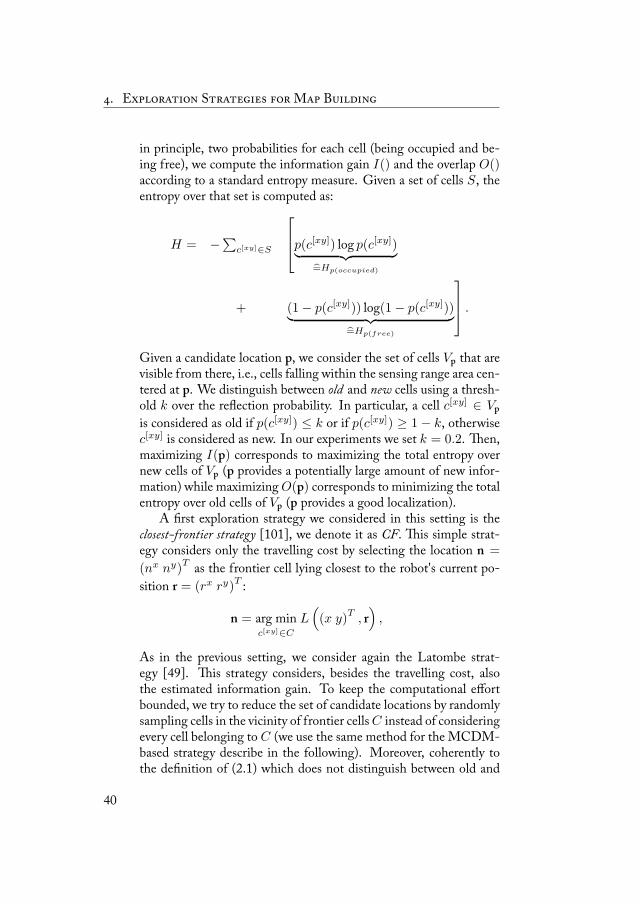
. E S M B

in principle, two probabilities for each cell (being occupied and be-ing free), we compute the information gain I() and the overlap O()according to a standard entropy measure. Given a set of cells S, theentropy over that set is computed as:

H = −∑

c[xy]∈S

p(c[xy]) log p(c[xy])︸ ︷︷ ︸=Hp(occupied)

+ (1− p(c[xy])) log(1− p(c[xy]))︸ ︷︷ ︸=Hp(free)

.

Given a candidate location p, we consider the set of cells Vp that arevisible from there, i.e., cells falling within the sensing range area cen-tered at p. We distinguish between old and new cells using a thresh-old k over the reflection probability. In particular, a cell c[xy] ∈ Vpis considered as old if p(c[xy]) ≤ k or if p(c[xy]) ≥ 1− k, otherwisec[xy] is considered as new. In our experiments we set k = 0.2. en,maximizing I(p) corresponds to maximizing the total entropy overnew cells of Vp (p provides a potentially large amount of new infor-mation) while maximizingO(p) corresponds to minimizing the totalentropy over old cells of Vp (p provides a good localization).

A first exploration strategy we considered in this setting is theclosest-frontier strategy [101], we denote it as CF. is simple strat-egy considers only the travelling cost by selecting the location n =

(nx ny)T as the frontier cell lying closest to the robot's current po-

sition r = (rx ry)T :

n = arg minc[xy]∈C

L((x y)

T, r),

As in the previous setting, we consider again the Latombe strat-egy [49]. is strategy considers, besides the travelling cost, alsothe estimated information gain. To keep the computational effortbounded, we try to reduce the set of candidate locations by randomlysampling cells in the vicinity of frontier cellsC instead of consideringevery cell belonging to C (we use the same method for the MCDM-based strategy describe in the following). Moreover, coherently tothe definition of (2.1) which does not distinguish between old and

40

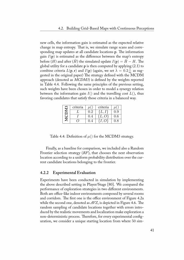
4.2. Building Grid-Based Maps with Continuous Perceptions

new cells, the information gain is estimated as the expected relativechange in map entropy. at is, we simulate range scans and corre-sponding map updates at all candidate locations p. e informationgain I(p) is estimated as the difference between the map's entropybefore (H) and after (H) the simulated update I(p) = H −H . eglobal utility for a candidate p is then computed by applying (2.1) tocombine criteria L(p, r) and I(p) (again, we set λ = 0.2 1

m as sug-gested in the original paper) e strategy defined with the MCDMapproach (denoted as MCDM3) is defined by the weights reportedin Table 4.4. Following the same principles of the previous setting,such weights have been chosen in order to model a synergy relationbetween the information gain I() and the travelling cost L(), thusfavoring candidates that satisfy those criteria in a balanced way.

MCDM3 criteria µ() criteria µ()

L 0.2 {L, I} 0.9I 0.4 {L,O} 0.6O 0.4 {I,O} 0.8

Table 4.4: Definition of µ() for the MCDM3 strategy.

Finally, as a baseline for comparison, we included also a RandomFrontier selection strategy (RF ), that chooses the next observationlocation according to a uniform probability distribution over the cur-rent candidate locations belonging to the frontier.

4.2.2 Experimental EvaluationExperiments have been conducted in simulation by implementingthe above described setting in Player/Stage [80]. We compared theperformance of exploration strategies in two different environments.Both are office-like indoor environments composed by several roomsand corridors. e first one is the office environment of Figure 4.2awhile the second one, denoted as AVZ, is depicted in Figure 4.6. erandom sampling of candidate locations together with errors intro-duced by the realistic movements and localization make exploration anon-deterministic process. erefore, for every experimental config-uration, we consider a unique starting location from where 50 sim-

41

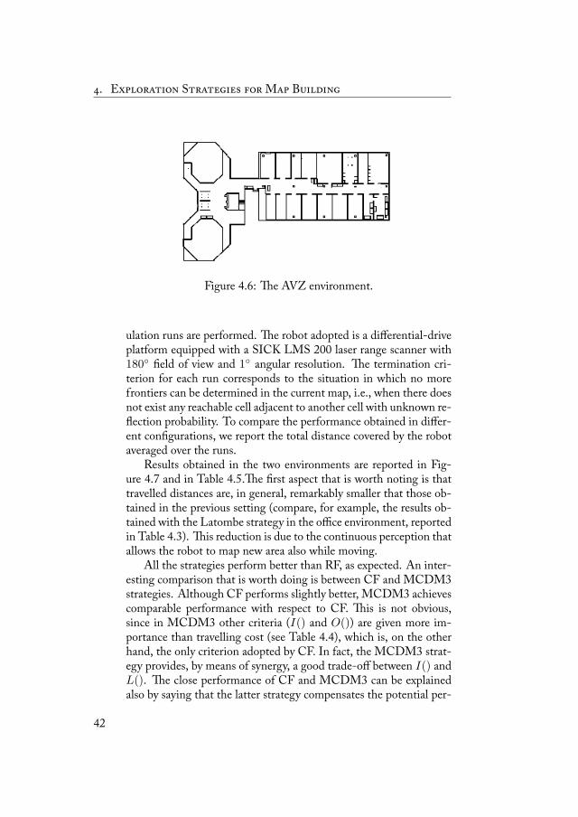
. E S M B

Figure 4.6: e AVZ environment.

ulation runs are performed. e robot adopted is a differential-driveplatform equipped with a SICK LMS 200 laser range scanner with180◦ field of view and 1◦ angular resolution. e termination cri-terion for each run corresponds to the situation in which no morefrontiers can be determined in the current map, i.e., when there doesnot exist any reachable cell adjacent to another cell with unknown re-flection probability. To compare the performance obtained in differ-ent configurations, we report the total distance covered by the robotaveraged over the runs.

Results obtained in the two environments are reported in Fig-ure 4.7 and in Table 4.5.e first aspect that is worth noting is thattravelled distances are, in general, remarkably smaller that those ob-tained in the previous setting (compare, for example, the results ob-tained with the Latombe strategy in the office environment, reportedin Table 4.3). is reduction is due to the continuous perception thatallows the robot to map new area also while moving.

All the strategies perform better than RF, as expected. An inter-esting comparison that is worth doing is between CF and MCDM3strategies. Although CF performs slightly better, MCDM3 achievescomparable performance with respect to CF. is is not obvious,since in MCDM3 other criteria (I() and O()) are given more im-portance than travelling cost (see Table 4.4), which is, on the otherhand, the only criterion adopted by CF. In fact, the MCDM3 strat-egy provides, by means of synergy, a good trade-off between I() andL(). e close performance of CF and MCDM3 can be explainedalso by saying that the latter strategy compensates the potential per-

42

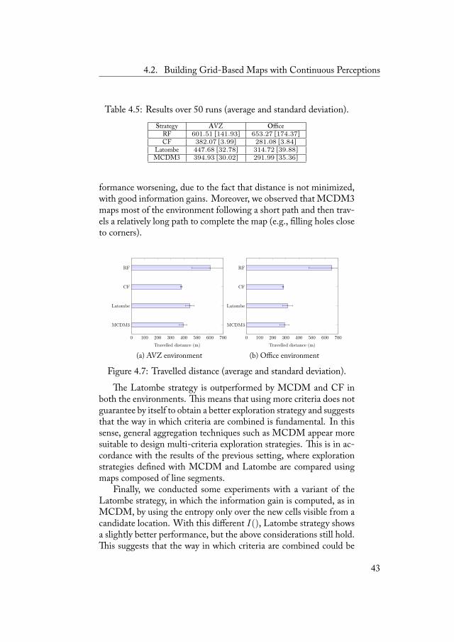
4.2. Building Grid-Based Maps with Continuous Perceptions

Table 4.5: Results over 50 runs (average and standard deviation).Strategy AVZ Office

RF 601.51 [141.93] 653.27 [174.37]CF 382.07 [3.99] 281.08 [3.84]

Latombe 447.68 [32.78] 314.72 [39.88]MCDM3 394.93 [30.02] 291.99 [35.36]

formance worsening, due to the fact that distance is not minimized,with good information gains. Moreover, we observed that MCDM3maps most of the environment following a short path and then trav-els a relatively long path to complete the map (e.g., filling holes closeto corners).

0 100 200 300 400 500 600 700

MCDM3

Latombe

CF

RF

Travelled distance (m)

(a) AVZ environment

0 100 200 300 400 500 600 700

MCDM3

Latombe

CF

RF

Travelled distance (m)

(b) Office environment

Figure 4.7: Travelled distance (average and standard deviation).

e Latombe strategy is outperformed by MCDM and CF inboth the environments. is means that using more criteria does notguarantee by itself to obtain a better exploration strategy and suggeststhat the way in which criteria are combined is fundamental. In thissense, general aggregation techniques such as MCDM appear moresuitable to design multi-criteria exploration strategies. is is in ac-cordance with the results of the previous setting, where explorationstrategies defined with MCDM and Latombe are compared usingmaps composed of line segments.

Finally, we conducted some experiments with a variant of theLatombe strategy, in which the information gain is computed, as inMCDM, by using the entropy only over the new cells visible from acandidate location. With this different I(), Latombe strategy showsa slightly better performance, but the above considerations still hold.is suggests that the way in which criteria are combined could be

43

. E S M B

even more important than the methods used to compute the criteriathemselves.

44

Exploration Strategies for Search and Rescue 5

In this chapter, we applyMCDMto search and rescue settings, wherethe primary objective is not only to build an accuratemap of the phys-ical space but to search the environment for locating the largest num-ber of victims in a limited amount of time. Differently from map-ping, search and rescue settings are characterized by time constraintsand battery limitations and generally require to privilege the amountof explored area (and, consequently, the possibility to find victims)over the map quality. Taking the step from mapping to search andrescue, we show how MCDM, due to its flexibility, can be easilyadopted also in this applicative context to obtain a good level of per-formance. In the situation we consider, a team of robots have tosearch an (initially unknown) environment for victims. Since no apriori knowledge about the possible locations of the victims is avail-able, we can safely reduce the problem of maximizing the number ofvictims found in a given time interval to the problem of maximizingthe amount of mapped area in the same time interval.

5.1 e AOJRF Controller

We implemented MCDM-based exploration strategies for searchand rescue applications in an existing robot controller. We looked atthe participants to the RoboCup Rescue Virtual Robots Competi-

45

. E S S R

tion where different teams compete in developing simulated roboticplatforms operating in Urban Search And Rescue scenarios simu-lated in USARSim [26] (an high fidelity 3D robot simulator). Froman analysis based on availability of code and performance obtainedin the competition, we selected the controller developed by Ams-terdam and Oxford Universities (Amsterdam Oxford Joint RescueForces1) for the 2009 competition [99]. e reasons for implement-ing MCDM-based exploration strategies in an existing controller arethat we can focus on the exploration strategies, exploiting existingand tested methods for navigation, localization, and mapping andthat we have a fair way to compare our exploration strategies withthat originally used in the controller.

e controller manages a team of robots. e robotic platformused is a Pioneer P3AT, whose basic model and sensors are providedwith the USARSim simulator. e map of the environment is main-tained by a base station (whose position is fixed in the environment)to which robots periodically send data. e map is two-dimensionaland is represented with two superimposed occupancy grids. e firstone is obtained with a small-range (typically 3 meters) scanner andconstitutes the safe area, i.e., the area where the robot can safelymove.e second one is obtained from maximum-range scans (typically 20meters) and constitutes the free area, i.e., the area which is believedto be free but not yet safe. Moreover, a clear area is also maintainedon the map as a subset of the safe area that has been checked for thepresence of victims (this task is accomplished with simulated sensorsfor victim detection). Given a map represented in this way, a set ofboundaries between safe and free regions are extracted and consid-ered as frontiers. For each frontier, the middle point is considered asa candidate location to reach. e utility of a candidate p is evaluatedby combining the following criteria:

• A(p) is the amount of free area beyond the frontier of p com-puted according to the free area occupancy grid;

• P (p) is the probability that the robot, once reached p, will beable to transmit data (such as the acquired data about the en-vironment or the locations of victims) to the base station, thiscriterion depends on the distance between p and the base sta-tion;

1http://www.jointrescueforces.eu/

46

5.2. Developing MCDM-based Strategies

• d(p, r) is the distance between p and current robot's position r,this criterion is calculated with two different methods: dEU (),using the Euclidean distance, and dPP (), using the exact valueof the distance returned by a path planner.

Given these criteria, the global utility for a candidate p is calculatedwith the following function:

u(p, r) =A(p)P (p)

d(p, r). (5.1)

We will refer to the exploration strategy using this global utility func-tion as the AOJRF strategy.

e assignment between robots and candidate locations is per-formed with the following algorithm:

1. compute the global utility u(p, r) of assigning each candidatep to each robot r using (5.1) where d(p, r) is calculated usingthe Euclidean distance dEU (),

2. find the pair (p∗, r∗) such that the previously computed utilityis maximum (p∗, r∗) = argmaxp,r u(p, r),

3. re-compute the distance of p∗ for r∗ using dPP ()with the pathplanner and update the utility of (p∗, r∗) using such exact valueinstead of the Euclidean distance (note that dPP () is alwayslarger, or equal, to dEU ()),

4. if (p∗, r∗) is still the best assignment, then assign robot r∗ tolocation p∗, otherwise go to Step 2,

5. eliminate robot r∗ and candidate p∗ and go to Step 2.

e reason behind the utility update of Step 3 is that computingdPP () requires a considerable amount of time. Doing this for allthe candidate locations and all robots would be not affordable in therescue competition, since a maximum exploration time of 20minutesis enforced.

5.2 DevelopingMCDM-based Strategies

We now describe the changes we made to the original controller toinclude ourMCDM-based strategies. e firstMCDM-based strat-egy we propose adopts the same criteria of AOJRF strategy (i.e., A,

47

. E S S R

P , and d as described above), but combines them with the MCDMapproach. Basically, we replace function (5.1) with function (3.1),with the weights reported in Tab. 5.1 (top). e resulting strategyis denoted as MCDMa. is strategy assigns more importance to Athan to P and d, pushing the robot to discover new areas, even cov-ering long distances or risking a loss of communication. e jointcontribution of d and P is inhibited by establishing redundancy be-tween them. On the other side, a synergy holds between d and A,privileging locations satisfying these criteria in a balanced way.

To applyMCDM, utilities have to be normalized (see Section 3.2).is forces us to compute the values of criteria for every candidatelocation. As already discussed, computing dPP () requires a largeamount of time. erefore, normalizing the updated utility in Step 3would require to determine the path for every candidate location,making the 20 minutes limit too strict to achieve an acceptable per-formance. To deal with this problem we use the following procedurein Step 3: once computed dPP (p

∗, r∗), we normalize it by using thepreviously calculated values dEU (p, r

∗) for other candidates.e second MCDM-based strategy we propose shows the flexi-

bility of MCDM in adding a new criterion, i.e., the robot's batteryremaining charge b. Considering the battery can improve explorationby preventing the robot from making decisions it cannot complete(e.g., selecting a location not reachable with the residual energy). Tocompute ub(p) we need an estimate of the energy spent for reach-ing p. We consider a very simple model in which the power limitis translated in a time limit, i.e., we assume that the robot can fullyoperate for 20 minutes, which is the time limit of the competition.In order to estimate the time needed to reach a location p we con-sider the corresponding path the robot should cover in terms of linearsegments and rotations. By approximating the linear and angular ve-locities of the robot as constants, we can derive acceptable estimatesof the time b(p) needed to reach p. Obviously, the smaller b(p) thebetter ub(p). Notice that, despite b strongly depends on d, it capturesalso the difficulty for covering a path (e.g., short but winding pathscould require lot of time and battery). We denote the obtained strat-egy as MCDMb, whose weights are reported in Tab. 5.1 (middle).

Finally, we show how MCDM can be also adopted for definingdifferent behaviors in exploration. Broadly speaking, given a set ofcriteria, a behavior is associated to a set of weights that drive the de-cisions of the robot during exploration. We introduce a MCDMw

48

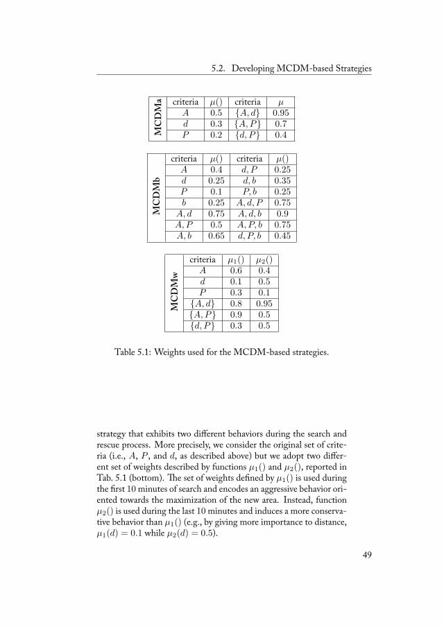
5.2. Developing MCDM-based Strategies

MCDMa criteria µ() criteria µ

A 0.5 {A, d} 0.95d 0.3 {A,P} 0.7P 0.2 {d, P} 0.4

MCDMb

criteria µ() criteria µ()A 0.4 d, P 0.25d 0.25 d, b 0.35P 0.1 P, b 0.25b 0.25 A, d, P 0.75

A, d 0.75 A, d, b 0.9A,P 0.5 A,P, b 0.75A, b 0.65 d, P, b 0.45

MCDMw

criteria µ1() µ2()A 0.6 0.4d 0.1 0.5P 0.3 0.1

{A, d} 0.8 0.95{A,P} 0.9 0.5{d, P} 0.3 0.5

Table 5.1: Weights used for the MCDM-based strategies.

strategy that exhibits two different behaviors during the search andrescue process. More precisely, we consider the original set of crite-ria (i.e., A, P , and d, as described above) but we adopt two differ-ent set of weights described by functions µ1() and µ2(), reported inTab. 5.1 (bottom). e set of weights defined by µ1() is used duringthe first 10minutes of search and encodes an aggressive behavior ori-ented towards the maximization of the new area. Instead, functionµ2() is used during the last 10minutes and induces a more conserva-tive behavior than µ1() (e.g., by giving more importance to distance,µ1(d) = 0.1 while µ2(d) = 0.5).

49

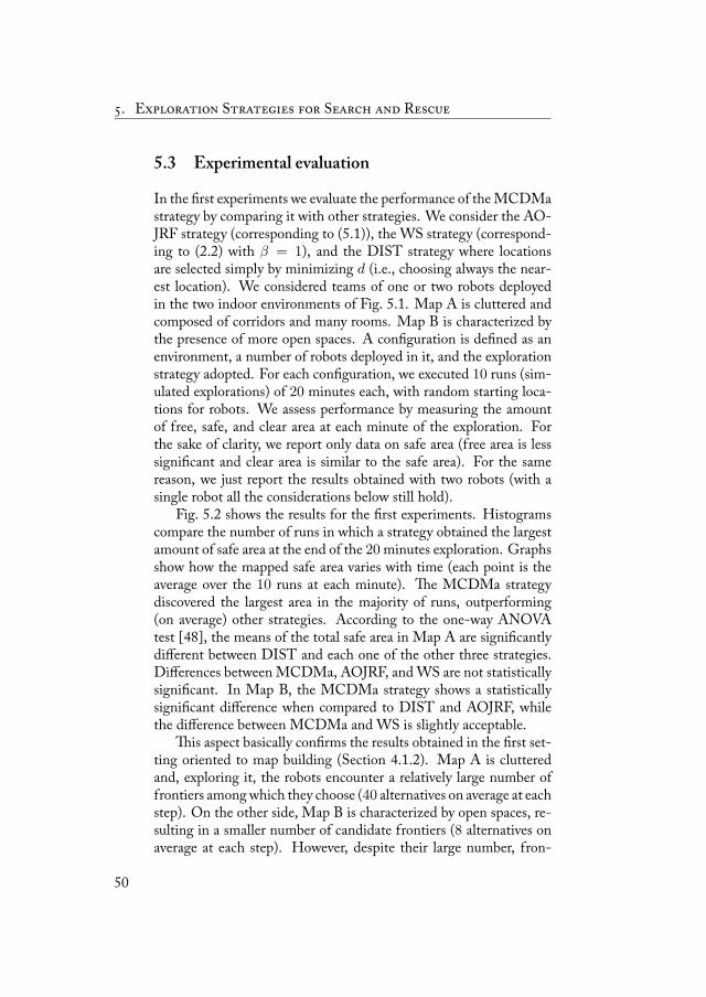
. E S S R

5.3 Experimental evaluation

In the first experiments we evaluate the performance of the MCDMastrategy by comparing it with other strategies. We consider the AO-JRF strategy (corresponding to (5.1)), the WS strategy (correspond-ing to (2.2) with β = 1), and the DIST strategy where locationsare selected simply by minimizing d (i.e., choosing always the near-est location). We considered teams of one or two robots deployedin the two indoor environments of Fig. 5.1. Map A is cluttered andcomposed of corridors and many rooms. Map B is characterized bythe presence of more open spaces. A configuration is defined as anenvironment, a number of robots deployed in it, and the explorationstrategy adopted. For each configuration, we executed 10 runs (sim-ulated explorations) of 20 minutes each, with random starting loca-tions for robots. We assess performance by measuring the amountof free, safe, and clear area at each minute of the exploration. Forthe sake of clarity, we report only data on safe area (free area is lesssignificant and clear area is similar to the safe area). For the samereason, we just report the results obtained with two robots (with asingle robot all the considerations below still hold).

Fig. 5.2 shows the results for the first experiments. Histogramscompare the number of runs in which a strategy obtained the largestamount of safe area at the end of the 20minutes exploration. Graphsshow how the mapped safe area varies with time (each point is theaverage over the 10 runs at each minute). e MCDMa strategydiscovered the largest area in the majority of runs, outperforming(on average) other strategies. According to the one-way ANOVAtest [48], the means of the total safe area in Map A are significantlydifferent between DIST and each one of the other three strategies.Differences between MCDMa, AOJRF, and WS are not statisticallysignificant. In Map B, the MCDMa strategy shows a statisticallysignificant difference when compared to DIST and AOJRF, whilethe difference between MCDMa and WS is slightly acceptable.

is aspect basically confirms the results obtained in the first set-ting oriented to map building (Section 4.1.2). Map A is clutteredand, exploring it, the robots encounter a relatively large number offrontiers amongwhich they choose (40 alternatives on average at eachstep). On the other side, Map B is characterized by open spaces, re-sulting in a smaller number of candidate frontiers (8 alternatives onaverage at each step). However, despite their large number, fron-

50

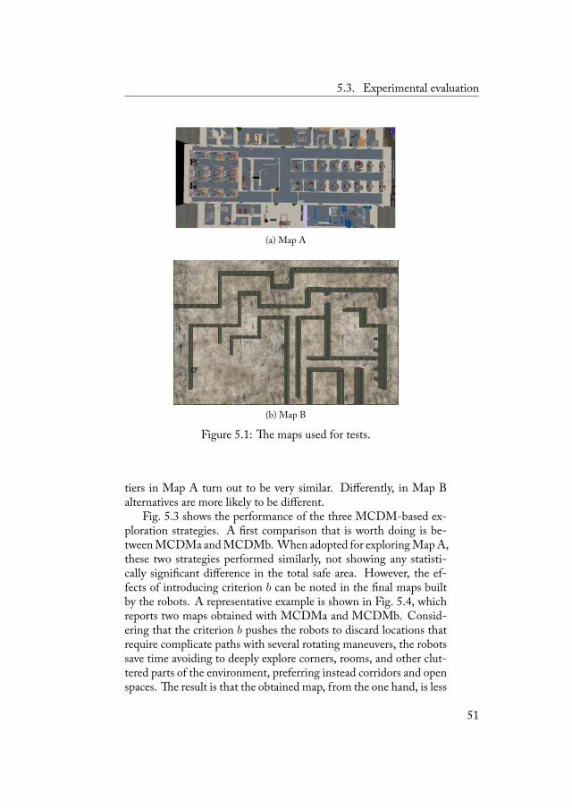
5.3. Experimental evaluation

(a) Map A

(b) Map B

Figure 5.1: e maps used for tests.

tiers in Map A turn out to be very similar. Differently, in Map Balternatives are more likely to be different.

Fig. 5.3 shows the performance of the three MCDM-based ex-ploration strategies. A first comparison that is worth doing is be-tweenMCDMa andMCDMb. When adopted for exploringMapA,these two strategies performed similarly, not showing any statisti-cally significant difference in the total safe area. However, the ef-fects of introducing criterion b can be noted in the final maps builtby the robots. A representative example is shown in Fig. 5.4, whichreports two maps obtained with MCDMa and MCDMb. Consid-ering that the criterion b pushes the robots to discard locations thatrequire complicate paths with several rotating maneuvers, the robotssave time avoiding to deeply explore corners, rooms, and other clut-tered parts of the environment, preferring instead corridors and openspaces. e result is that the obtained map, from the one hand, is less

51

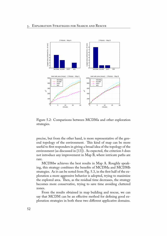
. E S S R

MCDMa AOJRF DIST WS0

1

2

3

4

5

Larg

est a

rea

achi

eved

(no

. of r

uns)

2 Robots − Map A

MCDMa AOJRF DIST WS0

1

2

3

4

5

6

7

8

Larg

est a

rea

achi

eved

(no

. of r

uns)

2 Robots − Map B

0 5 10 15 200

100

200

300

400

500total safe area (mean) − 2 Robots − Map A

minutes

m2

MCDMaAOJRFDISTWS

0 5 10 15 200

200

400

600

800

1000total safe area (mean) − 2 Robots − Map B

minutes

m2

MCDMaAOJRFDISTWS

Figure 5.2: Comparisons between MCDMa and other explorationstrategies.

precise, but from the other hand, is more representative of the gen-eral topology of the environment. is kind of map can be moreuseful to first responders in giving a broad idea of the topology of theenvironment (as discussed in [13]). As expected, the criterion b doesnot introduce any improvement in Map B, where intricate paths arerare.

MCDMw achieves the best results in Map A. Roughly speak-ing, this strategy combines the benefits of MCDMa and MCDMbstrategies. As it can be noted from Fig. 5.3, in the first half of the ex-ploration a more aggressive behavior is adopted, trying to maximizethe explored area. en, as the residual time decreases, the strategybecomes more conservative, trying to save time avoiding clutteredzones.

From the results obtained in map building and rescue, we cansay that MCDM can be an effective method for defining good ex-ploration strategies in both these two different applicative domains.

52

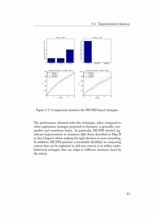
5.3. Experimental evaluation

MCDM MCDMb MCDMw0

1

2

3

Larg

est a

rea

achi

eved

(no

. of r

uns)

2 Robots − Map A

MCDM MCDMb MCDMw0

1

2

3

4

5

Larg

est a

rea

achi

eved

(no

. of r

uns)

2 Robots − Map B

0 5 10 15 200

100

200

300

400

500total safe area (mean) − 2 Robots − Map A

minutes

m2

MCDMMCDMbMCDMw

0 5 10 15 200

200

400

600

800

1000total safe area (mean) − 2 Robots − Map B

minutes

m2

MCDMMCDMbMCDMw

Figure 5.3: Comparisons between the MCDM-based strategies.

e performance obtained with this technique, when compared toother exploration strategies proposed in literature, is generally com-parable and sometimes better. In particular, MCDM showed sig-nificant improvements in situations (like those described in Map Bin this Chapter) where making the right decision is more rewarding.In addition, MCDM presents a remarkable flexibility in composingcriteria that can be exploited to add new criteria or to define multi-behavioral strategies that can adapt to different situations faced bythe robots.

53

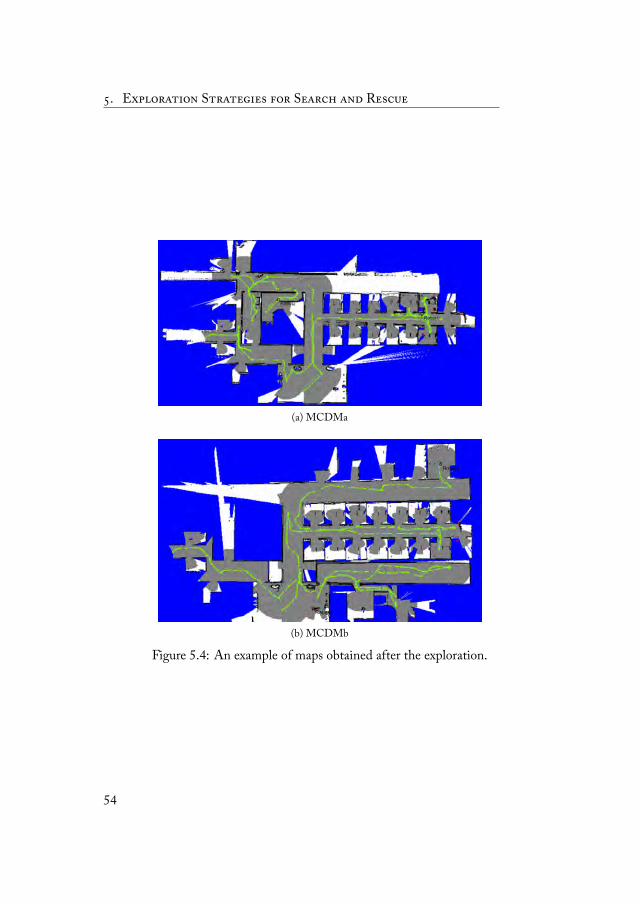
. E S S R

(a) MCDMa

(b) MCDMb

Figure 5.4: An example of maps obtained after the exploration.

54

Part II

Robotic Patrolling

e second part of this dissertation focuses on robotic patrolling.is task is performed by an autonomousmobile robot equipped withsensors that allow it to detect the presence of a possible intruderwithin some range. e robot moves within the environment andchecks for intrusions in order to find the intruder or, more generally,to avoid its entrance. e environment is typically fully known inadvance, according to a global knowledge situation, and the optimalstrategy can be computed offline. Decisions that are determined bythe navigation strategy (also denoted as patrolling strategy) amount tothe next environment's location where to check for the presence of anintruder. As it is evident, the patrolling strategy plays a critical rolein providing some protection level. Differently from autonomous ex-ploration, the patrolling scenario can be characterized by the interac-tion between the robot and another agent with contrasting objectives,i.e., an adversary. In this work we explicitly adopt this adversarialscenario by modeling a rational intruder whose objectives consist intrying to break the protection of the environment. e intruder ismodeled according to a worst case stance, by allowing it to observethe patrolling robot and to fully know its patrolling strategy. Differ-ent works in the field of security games modeled this situation witha leader-follower game, i.e., a particular class of games that prop-erly captures this kind of interaction where one agent knows in ad-vance the strategy employed by the other and uses this information tocompute its own strategy. e use of a game-theoretical frameworktranslates the concept of optimal patrolling strategy to that of equi-librium patrolling strategy. e optimal patrolling strategy, definedas the strategy that maximizes the revenue of the patrolling robot,can be found by solving the game and computing its equilibria. Inthis work we adopt this interactive decision-theoretical approach andwe show how it can be applied to patrolling settings in which theenvironment is modeled as an arbitrary graph. We propose an al-gorithm to find the optimal patrolling strategy and game-theoreticaltechniques to simplify the problem, reducing the computational timerequired for finding equilibria. We experimentally evaluate the algo-rithms' efficiency by solving a large number of instances and we assesstheir practical applicability by deploying the patrolling strategies ona realistic robot controller.

Approaches to Robotic Patrolling 6

In this chapter we present a survey of the main works on roboticpatrolling. We discuss how this problem has been addressed fromrobotic and game theoretical perspectives and how some works pre-sented in the operational research literature can be related to it.

6.1 Robotic Patrolling

Patrolling is an umbrella term that denotes several specific tasks. Abroad definition of patrolling is the act of walking or traveling aroundan area, at regular intervals, in order to protect or supervise it [70]. Manyscientific areas are involved in patrolling (e.g., hardware and softwarearchitectures [70]). Among them, we focus on algorithms for pro-ducing patrolling strategies. ese can be characterized according tothree main dimensions.

6.1.1 Problem's Dimensions

e first dimension concerns the representation of the patrolled area.It can be graph-based or continuous. In the case of graph-based repre-sentations, four types of topologies have been considered: perimeter(closed or open fence), fully connected (every vertex is connected to

59

. A R P

all the others), arbitrary, and arbitrary with targets (where the targetsconstitute a subset of vertices of interest).

e second dimension is the objective function of the patroller. Itcan explicitly take into account the presence of adversaries (adver-sarial) or not (non-adversarial). In the case it does not, objectivefunctions that have been studied include: coverage, where the aimis to cover at best a given area, frequency-based, where the aim is topatrol an area with a frequency that satisfies some properties, andother ad hoc objective functions or combinations of multiple objec-tive functions. In particular, four frequency-based approaches canbe identified: uniform (also called blanket time), where each locationof the area (e.g., a vertex) must be visited with the same given fre-quency, maximal average (also called average idleness1), where the aimis to maximize the average frequency of visit, maximal minimum (alsocalled worst idleness), where the aim is to maximize the minimumfrequency of visit, and location specific constraints, where each specificlocation has a specific lower bound over the frequency with which itshould be visited. In the case the presence of adversaries is explicitlyconsidered, there are two cases: expected utility with fixed adversary,where the expected utility of the patroller is maximized given a fixednon-rational model of the adversary, and expected utility with ratio-nal adversary, where the adversary is modeled as a rational decisionmaker.

e third dimension is the number of employed patrollers (corre-sponding to the resources available to the defender). Settings can besingle agent or multi agent.

6.1.2 Main RelatedWorks

Table 6.1 shows the classification of the main works on patrollingaccording to the above dimensions. e symbols ♦ and ? denote thecontributions we provide in Chapter 8 and Chapter 9, respectively.In the following we discuss in some detail the main related works onpatrolling reported in the table.

Carroll et al. [27] and Girard et al. [46] compose systems of mul-tiple air vehicles that patrol a border area. e environment is repre-sented as a continuous two-dimensional region that is divided in sub-regions. Each sub-region is assigned to an air vehicle that patrols it

1Idleness denotes the time between two successive visits of a vertex.

60

6.1. Robotic Patrolling

with a spiral trajectory. Also Guo et al. [53] consider multirobot pa-trolling of continuous environments. In this case, the environment ispartitioned in sub-regions using a Voronoi tessellation, robots are as-signed to sub-regions, and each robot patrols its sub-region in orderto have a complete coverage with minimum repeated coverage. emovements of a robot are determined by a neural network model thatallows to deal with dynamically varying environments.Martins-Filhoand Macau [72] exploit unpredictable chaotic trajectories to have arobot covering a continuous environment.

e work presented by Machado et al. [70] deals with multiagentpatrolling of vertices of graphs whose edges have unitary lengths.Several agent architectures are experimentally compared accordingto their effectiveness in minimizing the idleness. e approach hasbeen generalized by Almeida et al. [6], where edges with arbitrarylengths are considered, and analyzed from a theoretical perspectiveby Chevaleyre [29]. Moreover, Santana et al. [87] proposed rein-forcement learning as a way to coordinate patrolling agents and todrive them around the environment. e work of Elmaliach et al.[35] provides efficient algorithms to findmultiagent patrolling strate-gies in perimeters (closed and open fence) that minimize differentnotions of idleness, while Elmaliach et al. [34] propose a method toefficiently compute patrolling strategies minimizing the worst idle-ness in arbitrary graphs. Also the approach described by Yanovskiet al. [103] considers multiagent patrolling on graphs, but the goal isto patrol edges and not vertices. e objective function is the blan-ket time criterion. e proposed ant-based algorithm is shown toconverge to an Eulerian cycle in a finite number of steps and to re-visit edges with a finite period. A somehow similar work is discussedby Glad et al. [47]. Ruan et al. [83] and Marier et al. [71] consider amultiagent patrolling setting where the objective takes into accountmultiple criteria (e.g., idleness and distribution probabilities over theoccurrence of incidents) and is pursued exploiting MDP techniques.

e contribution we provide in Chapter 8 of this paper (denotedwith ♦ in Table 6.1) studies problems different from those studied bythe above frequency-basedworks. emain difference is that we lookfor a solution that satisfies a set of constraints without minimizing agiven function of the idleness.

Agmon et al. [2] provide an efficient (polynomial time) algorithmto solve perimeter multiagent patrolling settings in a game theoreticalfashion. A possible intruder can enter any vertex and is required to

61

. A R P

spend a given time (measured in turns and called penetration time) tohave success. e intruder and the patrollers have no preferences overthe vertices and the intruder will enter the vertex in which the prob-ability to be captured is minimum. e patrollers are synchronous.e problem is essentially a zero-sum game and the solution (i.e., thepatrolling strategy) is the patrollers' maxmin strategy. In [4] and [5]the model is extended by considering uncertainty over the sensing,while in [3] non-rational intruders are considered. Agmon [1] intro-duces the presence of events. Gatti [41] considers a fully connectedtopology graph where the patroller and the intruder can have differ-ent preferences over the vertices (i.e., the game is general sum) andprovides an efficient algorithm to compute the Nash equilibria of thegame. Sak et al. [86] assume three different fixed behaviors for ad-versaries: a random adversary, an adversary that always chooses topenetrate through a recently visited node, and an adversary that usesstatistical methods to predict the chances that a node will be visited.Authors experimentally evaluate by simulation the patrolling strate-gies, showing that no strategy is optimal for all the possible adver-saries. Amigoni et al. [10] study arbitrary topology graphs providingan on-line heuristic approach to find the agents' optimal strategies.

e contribution we provide in Chapter 9 of this paper (denotedwith ? in Table 6.1) generalizes both the works in [2] and [41] toarbitrary graphs with targets, but it is less computationally efficientfor the settings to which both approaches are applicable. Moreover,our contribution extends [86], capturing a rational adversary.

62

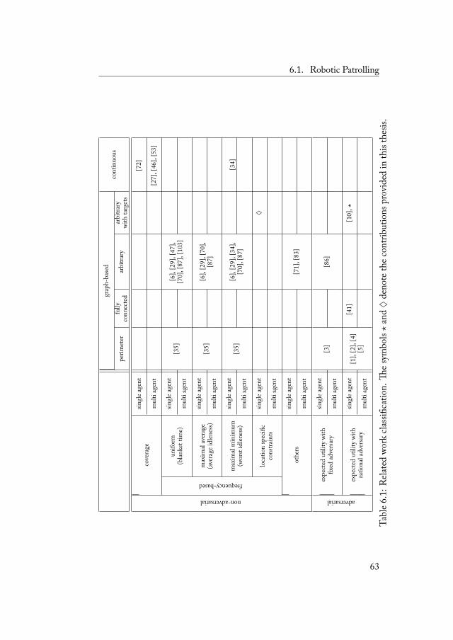
6.1. Robotic Patrolling

grap

h-ba

sed

cont

inuo

uspe

rimet

erfu

llyar

bitra

ryar

bitra

ryco

nnec

ted

with

targ

ets

non-adversarialco

vera

gesin

glea

gent

[72]

mul

tiag

ent

[27]

,[46

],[5

3]frequency-based

singl

eage

nt[3

5]un

iform

[6],

[29]

,[47

],(b

lanke

ttim

e)m

ulti

agen

t[7

0],[

87],

[103

]

singl

eage

nt[3

5]m

axim

alav

erag

e[6

],[2

9],[

70],

(ave

rage

idlen

ess)

mul

tiag

ent

[87]

singl

eage

nt[3

5]m

axim

alm

inim

um[6

],[2

9],[

34],

[34]

(wor

stid

lenes

s)m

ulti

agen

t[7

0],[

87]

singl

eage

nt♦

loca

tion

spec

ific

cons

train

tsm

ulti

agen

t

othe

rssin

glea

gent

[71]

,[83

]m

ulti

agen

t

adversarial

singl

eage

nt[3

][8

6]ex

pected

utili

tywi

thfix

edad

versar

ym

ulti

agen

t

singl

eage

nt[4

1][1

0],?

expe

cted

utili

tywi

th[1

],[2

],[4

]ra

tiona

ladv

ersa

rym

ulti

agen

t[5

]

Tabl

e6.1

:Rela

ted

work

classifi

catio

n.

esym

bols?

and♦

deno

teth

econ

tribu

tions

prov

ided

inth

isth

esis.

63

. A R P

6.2 Security Games

e approach we propose in this work resorts to game theory [40],modeling the patrolling scenario as two-player security game [76] be-tween a defender and an attacker. e basic ingredients of a securitygame are a number of targets, each with a value (potentially differ-ent for different players), and a number of resources available to thedefender to protect the targets from the attacker. In most situationsof interest, the resources available to the defender are not enoughto protect all the targets at once. is induces the defender to ran-domize (adopting a mixed strategy) over the possible assignments ofresources to targets to maximize its expected utility. On the otherhand, while the defender continuously and repeatedly protects thetargets, the attacker is assumed to be in the position to observe thedefender and derive a correct belief over its strategy. is last as-sumption places security games in the general class of leader-followergames where the leader, that commits to a strategy, is the defenderand the follower, that acts as a best responder given the leader's com-mitment, is the attacker.

Leader-follower games have been studied by von Stengel andZamir [100], who proposed the leader-follower equilibrium and dis-cussed some properties of this solution concept. In a leader-followerequilibrium, the leader plays the strategy that maximizes its expectedutility given that the follower observes this strategy and acts as a bestresponder.2 Although the leader-follower solution concept is appli-cable to games with an arbitrary number of players, it is particularlyappealing for two-player games. Indeed, von Stengel and Zamirshow that in these games any leader-follower equilibrium is neverworse than every Nash equilibrium. Hence, in some situations, theleader can receive an expected utility larger than that it receives withthe best Nash equilibrium. Another advantage is that, as we shalldiscuss below, computing a leader-follower equilibrium is much eas-ier than computing a Nash equilibrium and much larger games canbe solved.

Computing a leader-follower equilibrium is essentially a two-level mathematical programming problem where, in the first level,the leader's expected utility is maximized and, in the second one, the

2Technically speaking, the follower is not merely a best responder: at the equilib-rium, if it is indifferent among multiple actions, it must play the action that maximizesthe leader's expected utility.

64

6.2. Security Games

follower's expected utility is maximized. e basic work on com-puting a leader-follower equilibrium is by Conitzer and Sandholm[31]. By exploiting the fact that the follower, being a best respon-der, acts in pure strategies, they provide a multi-linear mathematicalprogramming (Multi-LP) formulation. Moreover, they show thatthe problem of computing a leader-follower equilibrium is polyno-mial in the size of the game (specifically, in the number of players'actions), when uncertainty is over the follower's payoffs, and it isNP-hard, when uncertainty is over the leader's payoffs.3 Paruchuriet al. [77] provide a mixed integer linear mathematical programming(MILP) formulation and show that it is very efficient (with respectto the Multi-LP formulation) when the number of follower's typesis large. Several works on security games have built on these two re-sults to produce more efficient algorithms by exploiting insights onthe game structure.

In the seminal work on security games, Paruchuri et al. [76] studythe problem of placing checkpoints to secure a number of targets.e defender's actions are plans of assignment of checkpoints to tar-gets over time (modeled with discrete turns), whereas the attacker'sactions are the intrusions in targets. An attack requires a numberof turns during which, if the defender assigns a checkpoint to the at-tacked target, the attacker is captured. e players act simultaneouslyat the initial turn, the defender implementing the plan of checkpointassignment to targets and the attacker intruding the chosen target.e authors assume that the attacker's payoffs are uncertain to thedefender and provide heuristics to solve large settings (withmany tar-gets and resources). e work has been refined in [77] and applied atthe Los Angels International Airport [63, 78]. Two other extensionsare worth citing: Kiekintveld et al. [64] study scheduling constraintsover the resource assignment and apply their algorithm to the FederalAir Marshal Service and Tsai et al. [95] introduce graph-based con-straints to capture the topology of a city. Yin et al. [104] show severalinteresting properties of security games, such as the interchangeabil-ity of the Nash equilibria and the equivalence between the maxminsolution and the Nash equilibria, and discuss the conditions underwhich the Nash equilibria are equivalent to the leader-follower equi-

3We recall that the problem of finding aNash equilibrium is PPAD-complete [88]and that P⊆PPAD⊆NP. Although we do not know whether or not P≡PPAD, it isgenerally believed that it is not and that searching for a Nash equilibrium requires anexponential time in the worst case.

65

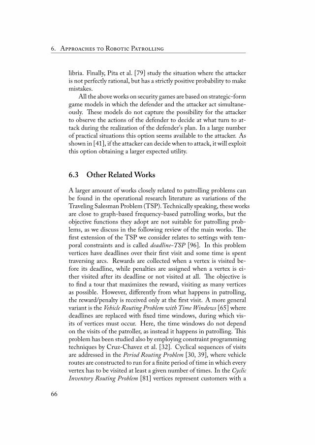
. A R P

libria. Finally, Pita et al. [79] study the situation where the attackeris not perfectly rational, but has a strictly positive probability to makemistakes.

All the above works on security games are based on strategic-formgame models in which the defender and the attacker act simultane-ously. ese models do not capture the possibility for the attackerto observe the actions of the defender to decide at what turn to at-tack during the realization of the defender's plan. In a large numberof practical situations this option seems available to the attacker. Asshown in [41], if the attacker can decide when to attack, it will exploitthis option obtaining a larger expected utility.

6.3 Other RelatedWorks

A larger amount of works closely related to patrolling problems canbe found in the operational research literature as variations of theTraveling SalesmanProblem (TSP). Technically speaking, these worksare close to graph-based frequency-based patrolling works, but theobjective functions they adopt are not suitable for patrolling prob-lems, as we discuss in the following review of the main works. efirst extension of the TSP we consider relates to settings with tem-poral constraints and is called deadline-TSP [96]. In this problemvertices have deadlines over their first visit and some time is spenttraversing arcs. Rewards are collected when a vertex is visited be-fore its deadline, while penalties are assigned when a vertex is ei-ther visited after its deadline or not visited at all. e objective isto find a tour that maximizes the reward, visiting as many verticesas possible. However, differently from what happens in patrolling,the reward/penalty is received only at the first visit. A more generalvariant is the Vehicle Routing Problem with Time Windows [65] wheredeadlines are replaced with fixed time windows, during which vis-its of vertices must occur. Here, the time windows do not dependon the visits of the patroller, as instead it happens in patrolling. isproblem has been studied also by employing constraint programmingtechniques by Cruz-Chavez et al. [32]. Cyclical sequences of visitsare addressed in the Period Routing Problem [30, 39], where vehicleroutes are constructed to run for a finite period of time in which everyvertex has to be visited at least a given number of times. In the CyclicInventory Routing Problem [81] vertices represent customers with a

66

6.3. Other Related Works

given demand rate and storage capacity. e objective is to find atour such that a distributor can repeatedly restock customers undersome constraints over visiting frequencies.

Finally, we note that problems similar to adversarial patrollinghave been studied in the pursuit-evasion (e.g., see the work of Isleret al. [62] and Vidal et al. [97]) and hide-and-seek fields (e.g., see thework of Halvorson et al. [54]). Roughly speaking, in both cases, ahider can hide itself in vertices of an arbitrary graph and a seeker canmove along the graph to seek the hider within a finite time. How-ever, some assumptions, including the fact that the hider's goal isonly to avoid capture and not to enter an area of interest, make thepursuit-evasion and the hide-and-seek problems not directly compa-rable with the patrolling problems we are considering.

67

e Patrolling Game 7

In this chapter we introduce our approach to compute navigationstrategies in the applicative context of robotic patrolling. We adopta game theoretical framework, where the adversary is explicitly con-sidered. Our contribution deals with a patrolling scenario where theintruder can observe the execution of the actions of the patroller andexploit this information to decide when to attack. With respect tothe works proposed in literature, we address adversarial patrolling onarbitrary graphs, while previous main results are either for perime-ter topologies with rational adversaries [2] or for arbitrary topologieswith non-rational adversaries [86].

In the following of this chapter, we describe our game modelthat captures our patrolling setting, we show that the appropriate so-lution concept to solve the game is the leader-follower equilibrium,we provide a basic solving algorithm according to the current stateof the art, and we discuss its limitations and the open problems. Inthe next chapters, we will propose solutions to these limitations andproblems.

7.1 AGameeoretical Framework for Patrolling

e patrolling situation we consider is characterized by the followingassumptions:

69

. T P G

• the environment to be patrolled is represented by an arbitrarygraph where all the arcs have the same length (as in [2]);

• some vertices, called targets, present some values;

• time is discretized in turns (as in [2, 76]);

• there is a single patrolling robot equipped with sensors (e.g.,a camera) and able to move along the graph and to detect thepresence of other agents in its current vertex;

• there is an intruder able to penetrate in a target of the environ-ment (as in [76, 77]);

• the intruder enters in a target directly appearing on it;

• an intrusion takes a given number of turns to be completed; thisnumber is in general different for each target (as in [2, 76]);

• the intruder can perfectly observe the patroller's strategy beforeentering a target, deriving a correct belief over it (as in [2, 76]);

• the patroller and the intruder are rational agents (as in [76,77]).

7.1.1 Patrolling SettingA patrolling setting is composed of the environment to be patrolledand of the sensing and action capabilities of the patroller and the in-truder.

A patrolling environment is described by a direct graph G =(V,A, T, v, d).1 V is the set of vertices to be patrolled. A is the setof arcs connecting the vertices. We often represent A by a functiona : V ×V → {0, 1}, where a(i, j) = 1means that there exists an arcdirected from vertex i to vertex j and a(i, j) = 0 means that thereis not. Given a vertex i, a vertex j is adjacent to i when a(i, j) = 1.T ⊆ V contains the targets having some value for both the patrollerand the intruder. Vertices that are not targets (in V \ T ) are part ofthe paths that the patroller traverses to move between targets. v is apair of functions (vp, vi) where vp : T → R+ assigns each target avalue for the patroller and vi : T → R+ assigns each target a value

1e graph representation of a real environment can be produced as in [67].

70

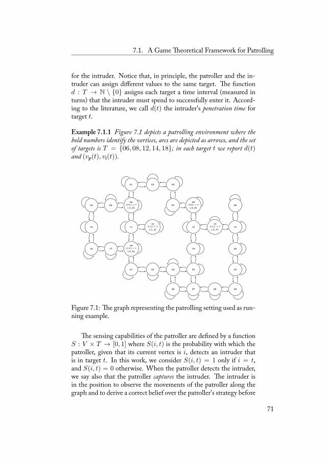
7.1. A Game eoretical Framework for Patrolling

for the intruder. Notice that, in principle, the patroller and the in-truder can assign different values to the same target. e functiond : T → N \ {0} assigns each target a time interval (measured inturns) that the intruder must spend to successfully enter it. Accord-ing to the literature, we call d(t) the intruder's penetration time fortarget t.

Example 7.1.1 Figure 7.1 depicts a patrolling environment where thebold numbers identify the vertices, arcs are depicted as arrows, and the setof targets is T = {06, 08, 12, 14, 18}; in each target t we report d(t)and (vp(t), vi(t)).

01 02 03

04 05

06d(06) = 9

(.1,.6)07

08d(08) = 8

(.3,.8)09

10 11

12d(12) = 9

(.1,.2)13

14d(14) = 9

(.2,.7)15

16 17

18d(18) = 8

(.3,.6)19 20

21 22 23 24 25

26 27 28 29

Figure 7.1: e graph representing the patrolling setting used as run-ning example.

e sensing capabilities of the patroller are defined by a functionS : V × T → [0, 1] where S(i, t) is the probability with which thepatroller, given that its current vertex is i, detects an intruder thatis in target t. In this work, we consider S(i, t) = 1 only if i = t,and S(i, t) = 0 otherwise. When the patroller detects the intruder,we say also that the patroller captures the intruder. e intruder isin the position to observe the movements of the patroller along thegraph and to derive a correct belief over the patroller's strategy before

71

. T P G

entering a target. is amounts to assume, according to a worst casestance, that the intruder knows the patroller's strategy before acting.

e action capabilities of the patroller are such that it spends oneturn to move between two adjacent vertices inG and patrol the arrivalvertex, while the intruder is able to appear directly in a target whenit decides to enter and to disappear directly from the target once theintrusion is completed. When an intrusion is attempted in target t,the intruder stays there and cannot do anything else for d(t) turns.During these turns the intruder can be detected (captured) by thepatroller.

7.1.2 GameModelA game is formally defined by a mechanism specifying the rules of thegame and the preferences of the agents over the outcomes and by thestrategies of the agents specifying their behavior during the game [40].

We model the patrolling scenario as a two-player multi-stagegame with imperfect information and infinite horizon [40], wherethe players are the patroller agent and the intruder agent.2 At eachstage of the game (corresponding to a turn), the patroller and theintruder act simultaneously. e patroller's available actions are de-noted by move(j) where j ∈ V is a vertex adjacent to the patroller'scurrent one. We assume that when action move(j) is played at turnk, then at turn k + 1 the patroller occupies vertex j and checks itfor the presence of the intruder. e intruder's available actions aredenoted by wait and enter(t) with t ∈ T . Playing action wait at turnk means not to attempt any intrusion for that turn. Playing actionenter(t) at turn k means to attempt an intrusion in target t and pre-vents the intruder from taking any other action in the time interval{k+1, . . . , k+d(t)−1}. e intruder's actions are not perfectly ob-servable and thus the patroller, when acting, does not know whetherthe intruder is currently within a target or it is still waiting to attack.e game has an infinite horizon, since the intruder is allowed to waitindefinitely outside the environment.

e possible outcomes of this game are:

• no-attack: when the intruder plays wait at every turn k, i.e., itnever attacks any target;

2Note that the game could be represented also as a partially-observable stochasticgame with infinite states.

72

7.1. A Game eoretical Framework for Patrolling

• intruder-capture: when the intruder plays enter(t) at turn k andthe patroller visits target t in the time interval I = {k, k +1, . . . , k + d(t)− 1} (and consequently detects the intruder);

• penetration-t: when the intruder plays enter(t) at turn k and thepatroller does not visit target t in the time interval I definedabove.

Example 7.1.2 Figure 7.2 reports a portion of the game tree for the set-ting of Figure 7.1, given that the initial position of the patroller is vertex01. Branches represent actions and players' information sets are depictedas dotted lines. Each turn of the game corresponds to two levels of the tree,where the patroller and the intruder take one action each.

patroller

move(01)

wait

move(0

1)

b

intruder-capture

enter(01)

ente

r(02)

move(0

1)

b

. . .

move(0

2)

wait

move(0

1)

ente

r(01)

move(0

1)

b

intruder-capture

enter(0

2)

. . .

move(06)

intruder

patroller patroller

. . .

. . . . . .

. . . . . . . . . . . . . . . . . . . . . . . . . . . . . . . . . . . .

Figure 7.2: A portion of the game tree for the patrolling setting ofFigure 7.1, with the patroller initially in 01.

Agents' utility functions over the outcomes are defined as follows.e patroller's utility function, denoted by up, is defined as the totalamount of preserved targets' value. Assuming that the patroller isrisk neutral, we have:

up(x) =

{∑i∈T vp(i) x = intruder-capture or no-attack∑i∈T\{t} vp(i) x = penetration-t

.

Notice that the patroller gets the same utility when the intruder iscaptured and when the intruder never enters. is is because, in thecase a utility surplus is given for capture, the patroller could prefer alottery between intruder-capture and penetration-t to no-attack. isbehavior is not reasonable, since the patroller's primary purpose in a

73

. T P G

typical patrolling setting is to preserve as much value as it can andnot necessarily capture the intruder. In the case of risk averse or riskseeking patroller, up should be defined as a concave or convex func-tion of the sum of the preserved values, respectively.

e intruder's utility function is denoted by ui. In case the in-truder is captured it gets a penalty, otherwise it gets the value of theattacked target. Assuming that the intruder is risk neutral, we have:

ui(x) =

0 x = no-attackvi(t) x = penetration-t−ε x = intruder-capture

,

where ε ∈ R+ is the penalty due to the capture. is is to saythat the status quo (i.e., no-attack) is better than being captured (i.e.,intruder-capture) for the intruder. In the case of risk averse or riskseeking intruder, ui should be a concave or convex function of theattacked target's value, respectively.

We denote byH the space of all the possible histories h of verticesvisited (or, equivalently, actions taken) by the patroller. For example,in Figure 7.1, given that the patroller starts from vertex 01, a possiblehistory is h = 〈01, 02, 03, 07, 08〉. We define the patroller's strategyas σp : H → ∆(V )where∆(V ) is a probability distribution over thevertices V or, equivalently, over the corresponding actions move(j).Given an history h ∈ H , the strategy σp gives the probability withwhich the patroller will move to vertices at the next turn. e pa-troller's strategy does not depend on the actions undertaken by theintruder, these being unobservable for the patroller. We can distin-guish between deterministic (pure) and non-deterministic (mixed) pa-trolling strategies. When σp is in pure strategies, assigning a prob-ability of one to a single vertex for each possible history h, we saythat the patrolling strategy is deterministic. Otherwise, we say thatthe patrolling strategy is non-deterministic. We define the intruder'sstrategy as σi : H → ∆(T ∪ {wait}) where ∆(T ∪ {wait}) is aprobability distribution over the vertices T (or, equivalently, over thecorresponding actions enter(t)) and the action wait.

Example 7.1.3 In Figure 7.1, a deterministic patrolling strategy couldprescribe the patroller to follow the cycle 〈04, 05, 06, 11, 18, 17, 16, 10, 04〉,while a non-deterministic patrolling strategy when the patroller is in ver-tex 01 after an history h could be:

74

7.2. Solution Concept

σp(h) =

01 with a probability of 0.2502 with a probability of 0.2506 with a probability of 0.5

.

An example of intruder's strategy is: play wait for all the histories whoselast vertex is not 04 and play enter(18) otherwise.

7.2 Solution Concept

e intruder's ability to observe the patroller's strategy and act onthe basis of such observation ''naturally'' induces a leader-followergame. In a leader-follower game the leader declares its strategy tothe follower that considers it when deciding its strategy. In the caseof patrolling, the patroller is the leader and the intruder is the fol-lower. is assumption amounts to suppose that the intruder canobserve the movements of the patroller and derive a correct belief onthe patrolling strategy. Indeed, the patroller, being observable, im-plicitly declares its strategy and the intruder considers the observedpatrolling strategy in deciding how to act. In [100], the authorsshow that in any two-player strategic-form game the leader nevergets worse by committing to a leader-follower equilibrium strategythan by playing a Nash equilibrium strategy. Since the game modeldescribed in the previous section is not properly a strategic-form one,the result in [100] is not directly applicable. However, we show in thenext sections that also in our case any equilibrium without commit-ment (discussed in Section 7.2.1) is never better than any equilibriumwith commitment (discussed in Section 7.2.2).

7.2.1 Solution Concept in Absence of any CommitmentWe consider the patroller's strategy in absence of any commitment.e appropriate solution concept for a multi-stage game with imper-fect information is the sequential equilibrium [68], which is a refine-ment of Nash equilibrium.3

3A sequential equilibrium is a pair (σ, µ) where σ is the agents' strategy profileand µ is a system of beliefs (it prescribes how agents update their beliefs during thegame). In a sequential equilibrium, the strategies are rational (sequential rationality)and the beliefs are consistent with the agents' optimal strategies (Kreps and Wilson'sconsistency).

75

. T P G

e presence of an infinite horizon complicates the study of thegame. With an infinite horizon, classic game theory studies a gameby introducing symmetries, e.g., an agent will repeat a given strategyevery k turns. Introducing symmetries in our game model amountsto force the agents' strategies to be defined on histories inH no longerthan a given value denoted by l.

Example 7.2.1 When l = 0, actions prescribed by the patroller's strategydo not depend on any previous action and the probability to visit a vertexis the same for all histories, namely for all the vertices where the patrolleris in. Notice that imposing l = 0 is not applicable for non-fully connectedgraph, where the set of actions available to the patroller actually dependson the current vertex. When l = 1, the patroller chooses its next action onthe basis of its last action (equivalently, the next action depends only onthe current vertex of the patroller). In this case, the patrolling strategy isMarkovian.

Unsurprisingly, when increasing the value of l, the patroller's ex-pected utility never decreases, because the patroller considers moreinformation to select its next action. Classical game theory [40]shows that games with infinite horizon admit a maximum length, sayl, of the symmetries such that the expected utility does not increaseanymore with l ≥ l and that usually l = 1 [40].4 In our model, thismeans that, when the patroller's strategy is defined on the last l ver-tices visited by the patroller, with l ≥ l the patroller's expected utilityis the same it receives with l = l. Notice that the number of possiblepure strategies σp(h) and σi(h) is O(nl), where n is the number ofvertices. erefore, we expect that, when increasing the value of l,the computational complexity for finding a patrolling strategy expo-nentially increases. In practical settings, the selection of a value for lis a trade-off between expected utility and computational effort.

7.2.2 Reduction to a Strategic-FormGame for a Given l

Given a value for l, our game can be reduced to a strategic-formgame by redefining the agents' actions and introducing constraintsthat force the patroller's strategies to be repeated every l turns (these

4A classical example is the Rubinstein's alternating-offers protocol [84], where abuyer and a seller can negotiate without any deadline. Here, the agents' strategies doesnot depend on the turn of the game and therefore l = 0.

76

7.3. Basic Algorithm

constraints will be formally defined in Section 7.3). e patroller'sactions are all the possible feasible probability assignments for {αh,i},where αh,i is the probability to execute action move(i) given historyh. e intruder's actions are enter-when(t, h), with t ∈ T andh ∈ H ,and stay-out. Action enter-when(t, h) corresponds to make wait un-til the patroller has followed history h and then to make enter(t);stay-out corresponds to make wait forever. With this representation,the two agents repeatedly act simultaneously, taking an action everyl turns of the original representation. Notice that the game does notdepend on the initial vertex of the patroller, both the patroller's andintruder's strategies not depending on it.

Example 7.2.2 Consider Figure 7.1. With l = 1, the available pa-trolling strategies are all the consistent probability assignments to {αi,j}where i, j ∈ V , while the intruder's actions are enter-when(t, j) witht ∈ T and j ∈ V and stay-out.

It can be easily observed that this reduced game is strategically equiv-alent to the original game and therefore every equilibrium of the re-duced game corresponds to an equilibrium of the original game. Be-ing a Nash equilibrium of a strategic-form game also a sequentialequilibrium, we have that a Nash equilibrium of the reduced gamecorresponds to a sequential equilibrium of the original game. Wecan now show that the leader-follower equilibrium is the appropriatesolution concept.

eorem 7.2.3 Given the game described above with a fixed l, the leadernever gets worse when committing to a leader-follower equilibrium strat-egy.

Proof. Since our game can be represented as a strategic-form gameand von Stengel andZamir [100] show that in any two-player strategic-form game the worst leader-follower equilibrium is not worse thanany Nash equilibrium for the leader, we have that the patroller canmaximize its expected utility by committing to a leader-follower equi-librium. �

7.3 Basic Algorithm

In order to find a leader-follower equilibrium of our patrolling game,we need to introduce the constraints that force the patroller's strate-

77

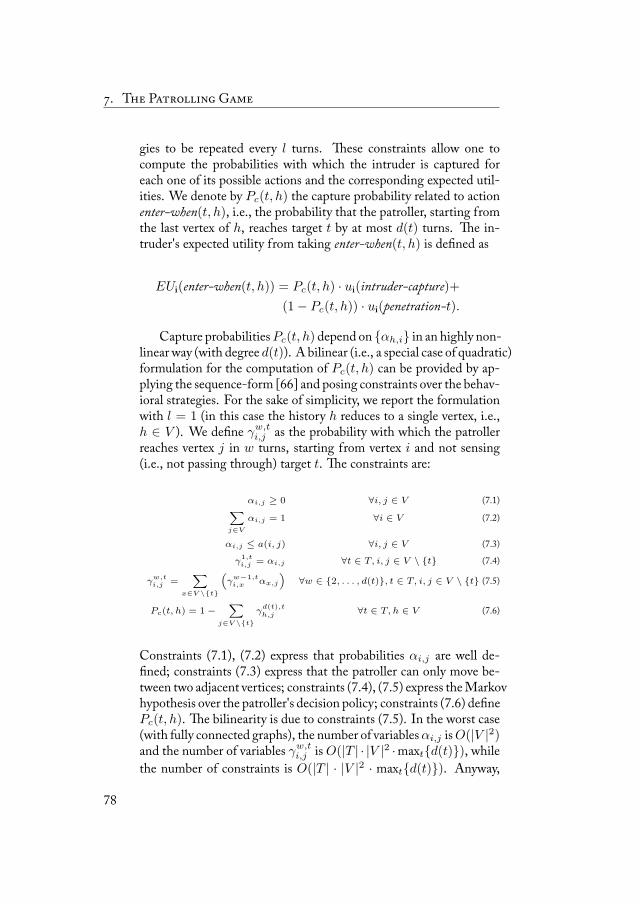
. T P G

gies to be repeated every l turns. ese constraints allow one tocompute the probabilities with which the intruder is captured foreach one of its possible actions and the corresponding expected util-ities. We denote by Pc(t, h) the capture probability related to actionenter-when(t, h), i.e., the probability that the patroller, starting fromthe last vertex of h, reaches target t by at most d(t) turns. e in-truder's expected utility from taking enter-when(t, h) is defined as

EUi(enter-when(t, h)) = Pc(t, h) · ui(intruder-capture)+(1− Pc(t, h)) · ui(penetration-t).

Capture probabilitiesPc(t, h) depend on {αh,i} in an highly non-linear way (with degree d(t)). A bilinear (i.e., a special case of quadratic)formulation for the computation of Pc(t, h) can be provided by ap-plying the sequence-form [66] and posing constraints over the behav-ioral strategies. For the sake of simplicity, we report the formulationwith l = 1 (in this case the history h reduces to a single vertex, i.e.,h ∈ V ). We define γw,t

i,j as the probability with which the patrollerreaches vertex j in w turns, starting from vertex i and not sensing(i.e., not passing through) target t. e constraints are:

αi,j ≥ 0 ∀i, j ∈ V (7.1)∑j∈V

αi,j = 1 ∀i ∈ V (7.2)

αi,j ≤ a(i, j) ∀i, j ∈ V (7.3)

γ1,ti,j = αi,j ∀t ∈ T, i, j ∈ V \ {t} (7.4)

γw,ti,j =

∑x∈V \{t}

(γw−1,ti,x αx,j

)∀w ∈ {2, . . . , d(t)}, t ∈ T, i, j ∈ V \ {t} (7.5)

Pc(t, h) = 1−∑

j∈V \{t}

γd(t),th,j ∀t ∈ T, h ∈ V (7.6)

Constraints (7.1), (7.2) express that probabilities αi,j are well de-fined; constraints (7.3) express that the patroller can only move be-tween two adjacent vertices; constraints (7.4), (7.5) express theMarkovhypothesis over the patroller's decision policy; constraints (7.6) definePc(t, h). e bilinearity is due to constraints (7.5). In the worst case(with fully connected graphs), the number of variablesαi,j isO(|V |2)and the number of variables γw,t

i,j is O(|T | · |V |2 ·maxt{d(t)}), whilethe number of constraints is O(|T | · |V |2 · maxt{d(t)}). Anyway,

78

7.3. Basic Algorithm

some variables and constraints of the above formulation are redun-dant and can be removed as shown in the following example.

Example 7.3.1 Consider action enter-when(14, 12) in Figure 7.1. Fo-cus on γ2,14

12,12, i.e., the probability associated with the event in which thepatroller starting from 12 reaches 12 after 2 turnswithout passing through14. If the event associated with γ2,14

12,12 happens, the probability withwhich the patroller reaches 14 by d(14) = 9 turns is zero, because thedistance between 12 and 14 is 9 and only 7 turns are left, and thereforethe intruder cannot be captured. e above constraints consider the possi-bility that the patroller moves from 12 to other vertices for 7 turns after theevent associated with γ2,14

12,12, introducing variables and constraints thatcould be safely omitted.

We modify the above constraints to make the computation ofPc(t, h) more efficient. To do this, we study the situation in whichthe intruder plays the corresponding action enter-when(t, h). Whenthe attack to t is started, the patroller is in vertex h (recall that, sincewe are considering l = 1, the history h reduces to a single vertex)and, in order to capture the intruder, it has to visit target t at leastonce in the following d(t) turns. In such scenario, a sufficient con-dition for a successful intrusion is the following: if after some turns,say ρ, the patroller has not yet visited t and occupies a vertex i suchthat ρ + dist(i, t) > d(t), then the intrusion has success.5 In otherwords, if the realization of the patroller's path drove it in a vertexfrom which t cannot be reached by its penetration time, the intrudercannot be captured at all. We can easily determine the minimumvalue of ρ for a target t when the patroller occupies a generic vertexi as ρ(i, t) = d(t)− dist(i, t) + 1. We can now reduce the numberof variables of the form γw,t

h,j that are included in the computation ofPc(t, h) by setting ρ(j, t) as the upper bound of index w. To do this,constraints (7.5) and (7.6) are replaced with the following ones:

5dist(i, j) is the shortest distance between two vertices i and j.

79

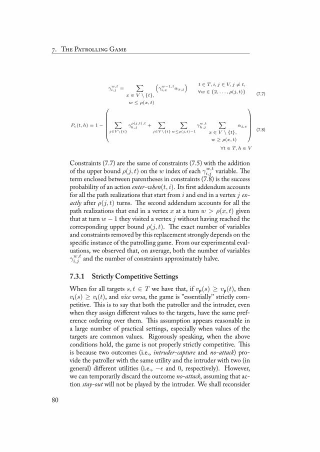
. T P G

γw,ti,j =

∑x ∈ V \ {t},w ≤ ρ(x, t)

(γw−1,ti,x αx,j

) t ∈ T, i, j ∈ V, j 6= t,

∀w ∈ {2, . . . , ρ(j, t)} (7.7)

Pc(t, h) = 1−

∑

j∈V \{t}

γρ(j,t),th,j +

∑j∈V \{t}

∑w≤ρ(j,t)−1

γw,th,j

∑x ∈ V \ {t},w ≥ ρ(x, t)

αj,x

∀t ∈ T, h ∈ V

(7.8)

Constraints (7.7) are the same of constraints (7.5) with the additionof the upper bound ρ(j, t) on the w index of each γw,t

i,j variable. eterm enclosed between parentheses in constraints (7.8) is the successprobability of an action enter-when(t, i). Its first addendum accountsfor all the path realizations that start from i and end in a vertex j ex-actly after ρ(j, t) turns. e second addendum accounts for all thepath realizations that end in a vertex x at a turn w > ρ(x, t) giventhat at turn w− 1 they visited a vertex j without having reached thecorresponding upper bound ρ(j, t). e exact number of variablesand constraints removed by this replacement strongly depends on thespecific instance of the patrolling game. From our experimental eval-uations, we observed that, on average, both the number of variablesγw,ti,j and the number of constraints approximately halve.

7.3.1 Strictly Competitive SettingsWhen for all targets s, t ∈ T we have that, if vp(s) ≥ vp(t), thenvi(s) ≥ vi(t), and vice versa, the game is ''essentially'' strictly com-petitive. is is to say that both the patroller and the intruder, evenwhen they assign different values to the targets, have the same pref-erence ordering over them. is assumption appears reasonable ina large number of practical settings, especially when values of thetargets are common values. Rigorously speaking, when the aboveconditions hold, the game is not properly strictly competitive. isis because two outcomes (i.e., intruder-capture and no-attack) pro-vide the patroller with the same utility and the intruder with two (ingeneral) different utilities (i.e., −ε and 0, respectively). However,we can temporarily discard the outcome no-attack, assuming that ac-tion stay-out will not be played by the intruder. We shall reconsider

80

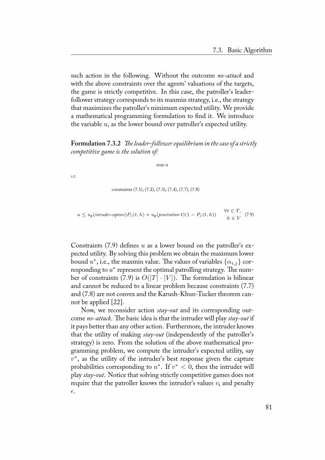
7.3. Basic Algorithm

such action in the following. Without the outcome no-attack andwith the above constraints over the agents' valuations of the targets,the game is strictly competitive. In this case, the patroller's leader-follower strategy corresponds to its maxmin strategy, i.e., the strategythat maximizes the patroller's minimum expected utility. We providea mathematical programming formulation to find it. We introducethe variable u, as the lower bound over patroller's expected utility.

Formulation 7.3.2 e leader-follower equilibrium in the case of a strictlycompetitive game is the solution of:

maxu

s.t.

constraints (7.1), (7.2), (7.3), (7.4), (7.7), (7.8)

u ≤ up(intruder-capture)Pc(t, h) + up(penetration-t)(1− Pc(t, h))∀t ∈ T,

h ∈ V(7.9)

Constraints (7.9) defines u as a lower bound on the patroller's ex-pected utility. By solving this problem we obtain the maximum lowerbound u∗, i.e., the maxmin value. e values of variables {αi,j} cor-responding to u∗ represent the optimal patrolling strategy. e num-ber of constraints (7.9) is O(|T | · |V |). e formulation is bilinearand cannot be reduced to a linear problem because constraints (7.7)and (7.8) are not convex and the Karush-Khun-Tucker theorem can-not be applied [22].

Now, we reconsider action stay-out and its corresponding out-come no-attack. e basic idea is that the intruder will play stay-out ifit pays better than any other action. Furthermore, the intruder knowsthat the utility of making stay-out (independently of the patroller'sstrategy) is zero. From the solution of the above mathematical pro-gramming problem, we compute the intruder's expected utility, sayv∗, as the utility of the intruder's best response given the captureprobabilities corresponding to u∗. If v∗ < 0, then the intruder willplay stay-out. Notice that solving strictly competitive games does notrequire that the patroller knows the intruder's values vi and penaltyε.

81

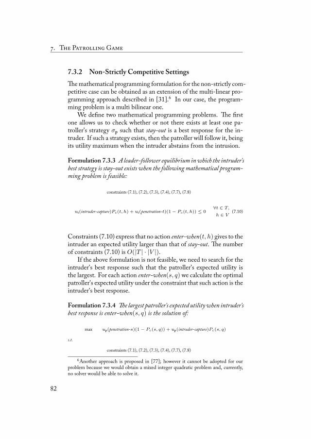
. T P G

7.3.2 Non-Strictly Competitive Settingsemathematical programming formulation for the non-strictly com-petitive case can be obtained as an extension of the multi-linear pro-gramming approach described in [31].6 In our case, the program-ming problem is a multi bilinear one.

We define two mathematical programming problems. e firstone allows us to check whether or not there exists at least one pa-troller's strategy σp such that stay-out is a best response for the in-truder. If such a strategy exists, then the patroller will follow it, beingits utility maximum when the intruder abstains from the intrusion.

Formulation 7.3.3 A leader-follower equilibrium inwhich the intruder'sbest strategy is stay-out exists when the following mathematical program-ming problem is feasible:

constraints (7.1), (7.2), (7.3), (7.4), (7.7), (7.8)

ui(intruder-capture)Pc(t, h) + ui(penetration-t)(1− Pc(t, h)) ≤ 0∀t ∈ T,

h ∈ V(7.10)

Constraints (7.10) express that no action enter-when(t, h) gives to theintruder an expected utility larger than that of stay-out. e numberof constraints (7.10) is O(|T | · |V |).

If the above formulation is not feasible, we need to search for theintruder's best response such that the patroller's expected utility isthe largest. For each action enter-when(s, q)we calculate the optimalpatroller's expected utility under the constraint that such action is theintruder's best response.

Formulation 7.3.4 e largest patroller's expected utilitywhen intruder'sbest response is enter-when(s, q) is the solution of:

max up(penetration-s)(1− Pc(s, q)) + up(intruder-capture)Pc(s, q)

s.t.

constraints (7.1), (7.2), (7.3), (7.4), (7.7), (7.8)

6Another approach is proposed in [77]; however it cannot be adopted for ourproblem because we would obtain a mixed integer quadratic problem and, currently,no solver would be able to solve it.

82

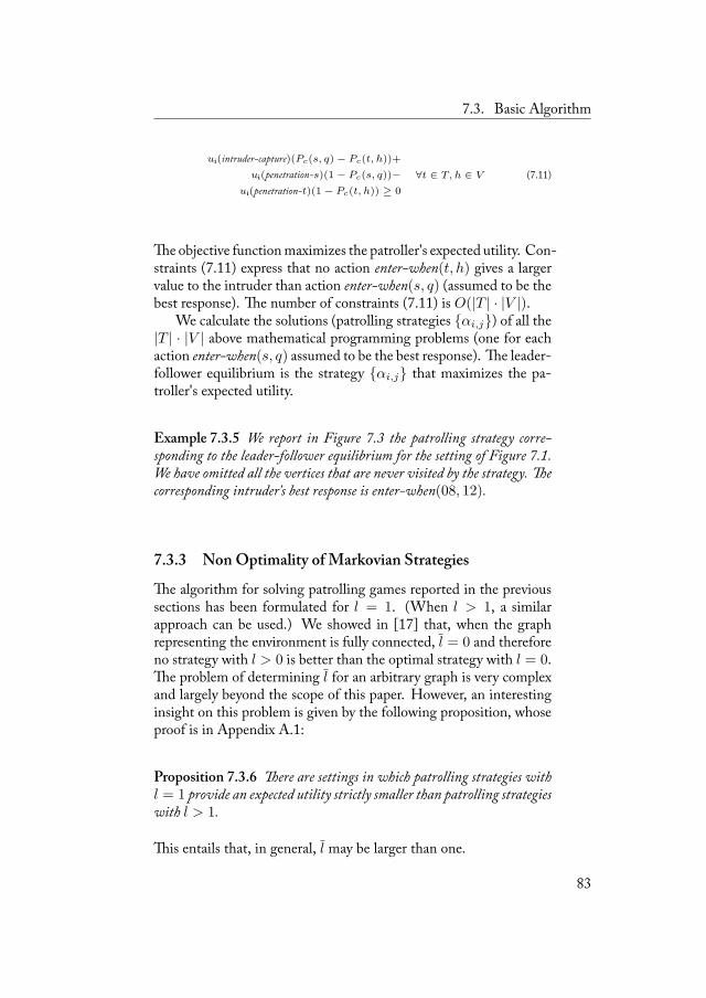
7.3. Basic Algorithm

ui(intruder-capture)(Pc(s, q)− Pc(t, h))+

ui(penetration-s)(1− Pc(s, q))−ui(penetration-t)(1− Pc(t, h)) ≥ 0

∀t ∈ T, h ∈ V (7.11)

eobjective functionmaximizes the patroller's expected utility. Con-straints (7.11) express that no action enter-when(t, h) gives a largervalue to the intruder than action enter-when(s, q) (assumed to be thebest response). e number of constraints (7.11) is O(|T | · |V |).

We calculate the solutions (patrolling strategies {αi,j}) of all the|T | · |V | above mathematical programming problems (one for eachaction enter-when(s, q) assumed to be the best response). e leader-follower equilibrium is the strategy {αi,j} that maximizes the pa-troller's expected utility.

Example 7.3.5 We report in Figure 7.3 the patrolling strategy corre-sponding to the leader-follower equilibrium for the setting of Figure 7.1.We have omitted all the vertices that are never visited by the strategy. ecorresponding intruder's best response is enter-when(08, 12).

7.3.3 NonOptimality of Markovian Strategies

e algorithm for solving patrolling games reported in the previoussections has been formulated for l = 1. (When l > 1, a similarapproach can be used.) We showed in [17] that, when the graphrepresenting the environment is fully connected, l = 0 and thereforeno strategy with l > 0 is better than the optimal strategy with l = 0.e problem of determining l for an arbitrary graph is very complexand largely beyond the scope of this paper. However, an interestinginsight on this problem is given by the following proposition, whoseproof is in Appendix A.1:

Proposition 7.3.6 ere are settings in which patrolling strategies withl = 1 provide an expected utility strictly smaller than patrolling strategieswith l > 1.

is entails that, in general, l may be larger than one.

83

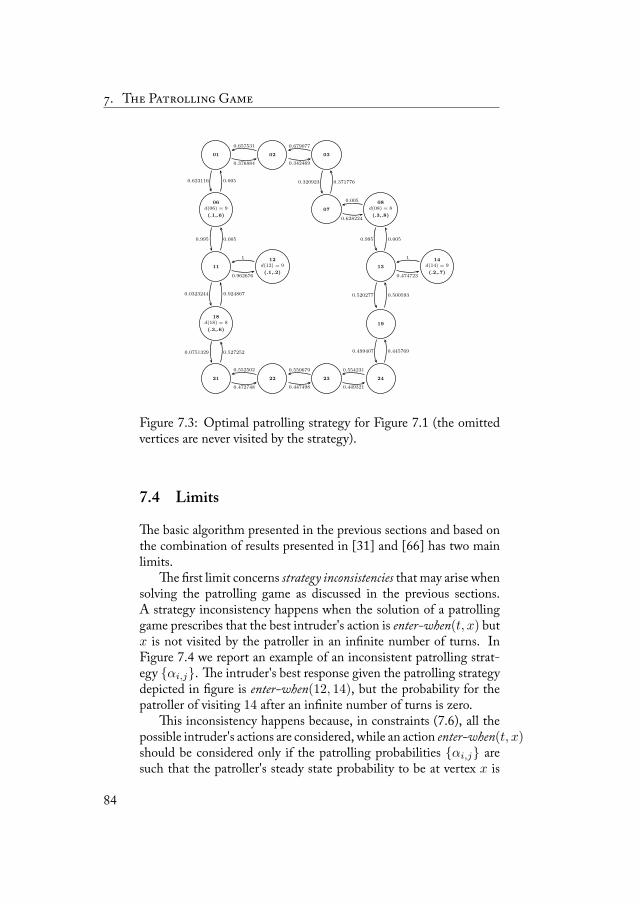
. T P G

01 02 03

06d(06) = 9

(.1,.6)07

08d(08) = 8

(.3,.8)

11

12d(12) = 9

(.1,.2)13

14d(14) = 9

(.2,.7)

18d(18) = 8

(.3,.6)19

21 22 23 24

0.376884

0.623116

0.657531

0.342469

0.679077

0.3209230.005

0.995

0.371776

0.628224

0.005

0.9950.005

0.962676

0.0323244

1

0.005

0.474723

0.520277

1

0.924867

0.0751329

0.500593

0.4994070.527252

0.472748

0.552502

0.447498

0.550679

0.449321

0.445769

0.554231

Figure 7.3: Optimal patrolling strategy for Figure 7.1 (the omittedvertices are never visited by the strategy).

7.4 Limits

e basic algorithm presented in the previous sections and based onthe combination of results presented in [31] and [66] has two mainlimits.

e first limit concerns strategy inconsistencies that may arise whensolving the patrolling game as discussed in the previous sections.A strategy inconsistency happens when the solution of a patrollinggame prescribes that the best intruder's action is enter-when(t, x) butx is not visited by the patroller in an infinite number of turns. InFigure 7.4 we report an example of an inconsistent patrolling strat-egy {αi,j}. e intruder's best response given the patrolling strategydepicted in figure is enter-when(12, 14), but the probability for thepatroller of visiting 14 after an infinite number of turns is zero.

is inconsistency happens because, in constraints (7.6), all thepossible intruder's actions are considered, while an action enter-when(t, x)should be considered only if the patrolling probabilities {αi,j} aresuch that the patroller's steady state probability to be at vertex x is

84

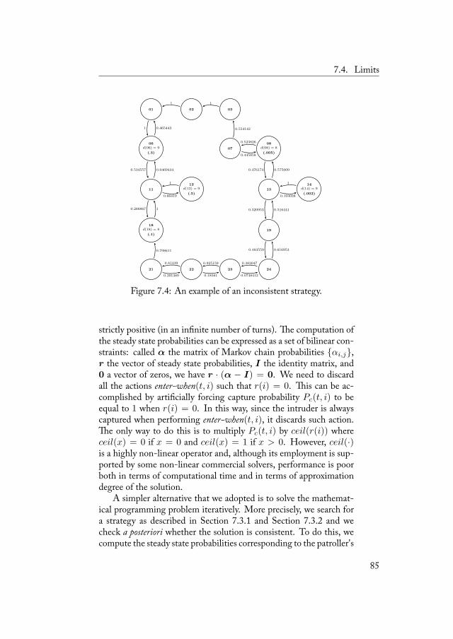
7.4. Limits

01 02 03

06d(06) = 9

(.3)07

08d(08) = 8

(.005)

11

12d(12) = 9

(.5)13

14d(14) = 9

(.002)

18d(18) = 8

(.1)19

21 22 23 24

1

1 1

0.465443

0.534557

0.554142

0.445858

0.523826

0.4761740.0469434

0.66419

0.288867

1

0.575009

0.104038

0.320953

1

1 0.516441

0.4835590.798611

0.201389

0.81439

0.18561

0.925159

0.0748412

0.616953

0.383047

Figure 7.4: An example of an inconsistent strategy.

strictly positive (in an infinite number of turns). e computation ofthe steady state probabilities can be expressed as a set of bilinear con-straints: called α the matrix of Markov chain probabilities {αi,j},r the vector of steady state probabilities, I the identity matrix, and0 a vector of zeros, we have r · (α − I) = 0. We need to discardall the actions enter-when(t, i) such that r(i) = 0. is can be ac-complished by artificially forcing capture probability Pc(t, i) to beequal to 1 when r(i) = 0. In this way, since the intruder is alwayscaptured when performing enter-when(t, i), it discards such action.e only way to do this is to multiply Pc(t, i) by ceil(r(i)) whereceil(x) = 0 if x = 0 and ceil(x) = 1 if x > 0. However, ceil(·)is a highly non-linear operator and, although its employment is sup-ported by some non-linear commercial solvers, performance is poorboth in terms of computational time and in terms of approximationdegree of the solution.

A simpler alternative that we adopted is to solve the mathemat-ical programming problem iteratively. More precisely, we search fora strategy as described in Section 7.3.1 and Section 7.3.2 and wecheck a posteriori whether the solution is consistent. To do this, wecompute the steady state probabilities corresponding to the patroller's

85

. T P G

strategy {αi,j} checking whether the steady state probability relatedto vertex i of the intruder's best response enter-when(t, i) is strictlypositive. If the solution is not consistent, then we remove vertex ifrom the graph. In the case removing i makes the resulting graphdisconnected, we remove also the component that does not containt. Its removal is safe because the intruder would never enter possibletargets in this component. en we attempt again to solve the newlyobtained patrolling setting.

e second important limit of the algorithm is its computationalhardness for solving realistically large game instances. In general,solving non-linear mathematical programming problems requires re-markable computational efforts. As we shall discuss in our experi-mental evaluations, only small settings (with respect to the number ofvertices and targets) can be solved with l = 1 and, when l > 1, evensmall instances become intractable. e computational time growsexponentially in the size (in terms of variables and constraints) of theproblem: called s the size of themathematical programming problemwith l = 1, the size with an arbitrary l is sl. is fact has two conse-quences. From the one hand, the limited scalability with respect tothe settings' size prevents the model from being applied to practicalscenarios even with l = 1. From the other hand, the practical im-possibility of increasing the value of l precludes the opportunity tofind more effective patrolling strategies, whose existence is suggestedby Proposition 7.3.6. To improve scalability and solving large gameinstances, we propose two approaches. In the first one (Chapter 8),we limit the generality of the solution by looking only for determin-istic (pure) strategies. We show that the limit on the value of l can beovercome in the specific case of deterministic strategies. Note that, ifthe equilibrium of a patrolling game admits a deterministic strategyσp for an arbitrary value of l such that the associated intruder's bestresponse is stay-out, then σp can be efficiently found by exploiting thestructure of the problem, avoiding mathematical programming andreducing the computational burden. is is the primary reason forwhich the computation of an equilibrium in deterministic strategiesis treated as a separate problem with respect to the computation ofan equilibrium in non-deterministic strategies. e second approach(Chapter 9) is based on the idea of simplifying the patrolling settingby introducing a pre-processing phase that eliminates variables andconstraints, while preserving the game theoretical consistency andthe solution optimality.

86

Deterministic Patrolling Strategies 8

Markovian strategies with l = 1 are, in general, non optimal. As dis-cussed in Section 7.3.3, increasing the value of the history length lcan led to better solutions in terms of expected utility to the patroller.However, the main difficulty in relaxing the Markovian assumptionresides in computational intractability. In this chapter, we describehow to overcome this limitation by exploiting the problem's struc-ture at the cost of restricting the solution's generality. We limit ourattention to deterministic (or pure) strategies that for each possiblehistory h assign a probability of one to an unique vertex (recall Sec-tion 7.1). We show that when limiting the search to this kind ofstrategies the structure of the problem can be effectively exploited todesign an algorithm that does not depend on the particular value of l.More precisely, we provide a formulation of the problem of finding adeterministic patrolling strategy in a constraint programming fash-ion, we analyze its complexity, and we propose and efficient solvingalgorithm.

8.1 Finding a Deterministic Strategy

Adeterministic patrolling strategyσp can be conveniently representedas a sequence of vertices. is representation does not depend on thevalue of l and, consequently, we allow l to assume arbitrary values.

87

. D P S

We are interested in finding (if it exists) a deterministic strategy suchthat the intruder's best response is stay-out and, as a consequence,such that the utility of the patroller is maximum. is strategy musthave the following property: when it is adopted by the patroller, eachtarget t is left uncovered for a number of turns not larger than its pen-etration time d(t) and thus every action enter-when(t, j)would resultin a certain capture for the intruder. Obviously, if this strategy exists,the patroller does not need to resort to randomization. Accordingto the classification proposed in Chapter 6, this solution belongs tothe class of frequency-based approaches with location specific con-straints.

Without loss of generality, a deterministic strategy can be definedonly on targets, assuming that the patroller will move between twotargets along the shortest path. We omit the proof, being trivial. isallows us to reduce drastically the space of search excluding all thevertices that are not targets. We reduce graph G = (V,A, T, v, d)to a weighted graph G′ = (T,A′, w, d), where targets T are thevertices of G′; A′ is the set of arcs connecting the targets defined asa function a′ : T × T → {0, 1} and derived from set A as follows:for every pair of targets i, j ∈ T and i 6= j, a′(i, j) = 1 if at leastone of the shortest paths connecting i to j in G does not visit anyother target, a′(i, j) = 0 otherwise; w is a weight function definedas w : T × T → N \ {0} where w(i, j) is the length of the shortestpath between i and j in G (w(i, j) is defined only when a′(i, j) = 1and represents the number of turns the patroller spends for goingfrom target i to target j along the shortest path); and d is the samefunction as defined in G. e reduction from G to G′ can be easilyaccomplished by applying Dijkstra's algorithm to every pair of targetsin G. For the sake of presentation, from here on we denote as σ adeterministic patrolling strategy over G′ and we refer to vertices ofG′, instead of targets.

Example 8.1.1 Consider the graph reported in Figure 7.1. e corre-sponding reduced graph G′ is reported in Figure 8.1a. G′ is composed ofonly 5 vertices. (e graph in Figure 8.1b differs from that in Figure 8.1ain the values of penetration times; we shall use it as example in the fol-lowing sections.)

We formally define the problem of searching for a determinis-tic strategy. Notice that pure strategy equilibria are usually found by

88

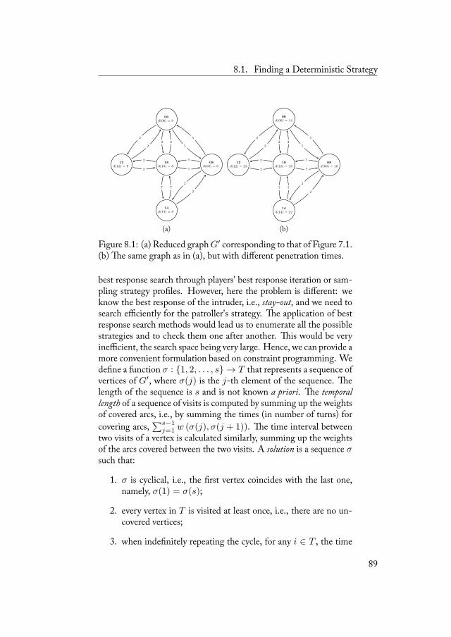
8.1. Finding a Deterministic Strategy

06d(06) = 9

12d(12) = 9

18d(18) = 8

08d(08) = 8

14d(14) = 9

2

22 2

5

5

2

2 7

7

772

2

(a)

06d(06) = 14

12d(12) = 23

18d(18) = 18

08d(08) = 18

14d(14) = 22

2

22 2

5

5

2

2 7

7

772

2

(b)

Figure 8.1: (a) Reduced graphG′ corresponding to that of Figure 7.1.(b) e same graph as in (a), but with different penetration times.

best response search through players' best response iteration or sam-pling strategy profiles. However, here the problem is different: weknow the best response of the intruder, i.e., stay-out, and we need tosearch efficiently for the patroller's strategy. e application of bestresponse search methods would lead us to enumerate all the possiblestrategies and to check them one after another. is would be veryinefficient, the search space being very large. Hence, we can provide amore convenient formulation based on constraint programming. Wedefine a function σ : {1, 2, . . . , s} → T that represents a sequence ofvertices of G′, where σ(j) is the j-th element of the sequence. elength of the sequence is s and is not known a priori. e temporallength of a sequence of visits is computed by summing up the weightsof covered arcs, i.e., by summing the times (in number of turns) forcovering arcs,

∑s−1j=1 w (σ(j), σ(j + 1)). e time interval between

two visits of a vertex is calculated similarly, summing up the weightsof the arcs covered between the two visits. A solution is a sequence σsuch that:

1. σ is cyclical, i.e., the first vertex coincides with the last one,namely, σ(1) = σ(s);

2. every vertex in T is visited at least once, i.e., there are no un-covered vertices;

3. when indefinitely repeating the cycle, for any i ∈ T , the time

89

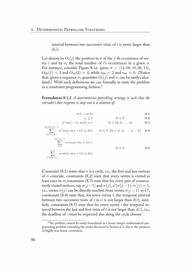
. D P S

interval between two successive visits of i is never larger thand(i).

Let denote by Oi(j) the position in σ of the j-th occurrence of ver-tex i and by oi the total number of i's occurrences in a given σ.For instance, consider Figure 8.1a: given σ = 〈14, 08, 18, 08, 14〉,O08(1) = 2 and O08(2) = 4, while o08 = 2 and o06 = 0. (Noticethat, given a sequence σ, quantities Oi(j) and oi can be easily calcu-lated.) With such definitions we can formally re-state the problemin a constraint programming fashion.1

Formulation 8.1.2 A deterministic patrolling strategy σ such that theintruder's best response is stay-out is a solution of:

σ(1) = σ(s) (8.1)oi ≥ 1 ∀i ∈ T (8.2)

a′(σ(j − 1), σ(j)) = 1 ∀j ∈ {2, 3, . . . , s} (8.3)

Oi(k+1)−1∑j=Oi(k)

w (σ(j), σ(j + 1)) ≤ d(i) ∀i ∈ T, ∀k ∈ {1, 2, . . . , oi − 1} (8.4)

Oi(1)−1∑j=1

w (σ(j), σ(j + 1))+

s−1∑j=Oi(oi)

w (σ(j), σ(j + 1)) ≤ d(i)

∀i ∈ T (8.5)

Constraint (8.1) states that σ is a cycle, i.e., the first and last verticesof σ coincide; constraints (8.2) state that every vertex is visited atleast once in σ; constraints (8.3) state that for every pair of consecu-tively visited vertices, say σ(j−1) and σ(j), a′(σ(j−1), σ(j)) = 1,i.e., vertex σ(j) can be directly reached from vertex σ(j − 1) in G′;constraints (8.4) state that, for every vertex i, the temporal intervalbetween two successive visits of i in σ is not larger than d(i); simi-larly, constraints (8.5) state that for every vertex i the temporal in-terval between the last and first visits of i is not larger than d(i), i.e.,the deadline of i must be respected also along the cycle closure.

1e problem cannot be easily formulated as a linear integer mathematical pro-gramming problem extending the works discussed in Section 6.3, due to the presenceof highly non-linear constraints.

90

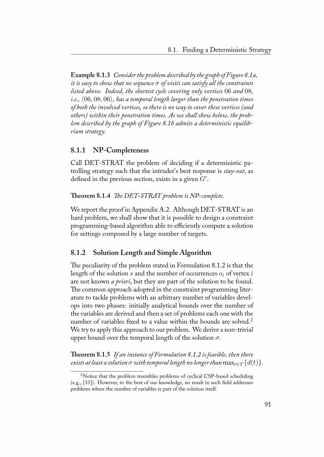
8.1. Finding a Deterministic Strategy

Example 8.1.3 Consider the problem described by the graph of Figure 8.1a,it is easy to show that no sequence σ of visits can satisfy all the constraintslisted above. Indeed, the shortest cycle covering only vertices 06 and 08,i.e., 〈06, 08, 06〉, has a temporal length larger than the penetration timesof both the involved vertices, so there is no way to cover these vertices (andothers) within their penetration times. As we shall show below, the prob-lem described by the graph of Figure 8.1b admits a deterministic equilib-rium strategy.

8.1.1 NP-CompletenessCall DET-STRAT the problem of deciding if a deterministic pa-trolling strategy such that the intruder's best response is stay-out, asdefined in the previous section, exists in a given G′.

eorem 8.1.4 e DET-STRAT problem is NP-complete.

We report the proof in Appendix A.2. Although DET-STRAT is anhard problem, we shall show that it is possible to design a constraintprogramming-based algorithm able to efficiently compute a solutionfor settings composed by a large number of targets.

8.1.2 Solution Length and Simple Algorithme peculiarity of the problem stated in Formulation 8.1.2 is that thelength of the solution s and the number of occurrences oi of vertex iare not known a priori, but they are part of the solution to be found.e common approach adopted in the constraint programming liter-ature to tackle problems with an arbitrary number of variables devel-ops into two phases: initially analytical bounds over the number ofthe variables are derived and then a set of problems each one with thenumber of variables fixed to a value within the bounds are solved.2We try to apply this approach to our problem. We derive a non-trivialupper bound over the temporal length of the solution σ.

eorem 8.1.5 If an instance of Formulation 8.1.2 is feasible, then thereexists at least a solutionσwith temporal length no longer thanmaxt∈T {d(t)}.

2Notice that the problem resembles problems of cyclical CSP-based scheduling(e.g., [33]). However, to the best of our knowledge, no result in such field addressesproblems where the number of variables is part of the solution itself.

91

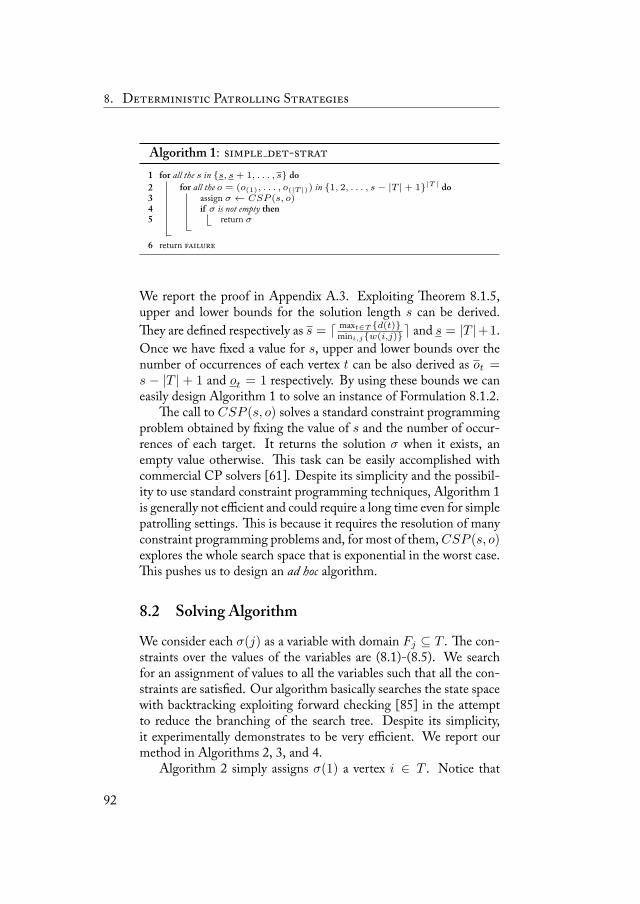
. D P S

Algorithm 1: -for all the s in {s, s + 1, . . . , s} do1

for all the o = (o(1), . . . , o(|T |)) in {1, 2, . . . , s− |T |+ 1}|T | do2assign σ ← CSP (s, o)3if σ is not empty then4

return σ5

return 6

We report the proof in Appendix A.3. Exploiting eorem 8.1.5,upper and lower bounds for the solution length s can be derived.ey are defined respectively as s = d maxt∈T {d(t)}

mini,j{w(i,j)}e and s = |T |+1.Once we have fixed a value for s, upper and lower bounds over thenumber of occurrences of each vertex t can be also derived as ot =s − |T | + 1 and ot = 1 respectively. By using these bounds we caneasily design Algorithm 1 to solve an instance of Formulation 8.1.2.

e call to CSP (s, o) solves a standard constraint programmingproblem obtained by fixing the value of s and the number of occur-rences of each target. It returns the solution σ when it exists, anempty value otherwise. is task can be easily accomplished withcommercial CP solvers [61]. Despite its simplicity and the possibil-ity to use standard constraint programming techniques, Algorithm 1is generally not efficient and could require a long time even for simplepatrolling settings. is is because it requires the resolution of manyconstraint programming problems and, for most of them,CSP (s, o)explores the whole search space that is exponential in the worst case.is pushes us to design an ad hoc algorithm.

8.2 Solving Algorithm

We consider each σ(j) as a variable with domain Fj ⊆ T . e con-straints over the values of the variables are (8.1)-(8.5). We searchfor an assignment of values to all the variables such that all the con-straints are satisfied. Our algorithm basically searches the state spacewith backtracking exploiting forward checking [85] in the attemptto reduce the branching of the search tree. Despite its simplicity,it experimentally demonstrates to be very efficient. We report ourmethod in Algorithms 2, 3, and 4.

Algorithm 2 simply assigns σ(1) a vertex i ∈ T . Notice that

92

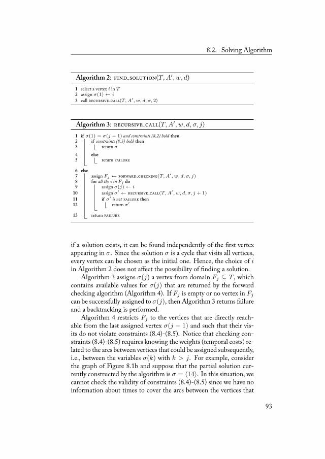
8.2. Solving Algorithm

Algorithm 2: (T,A′, w, d)select a vertex i in T1assign σ(1)← i2call (T,A′, w, d, σ, 2)3

Algorithm 3: (T,A′, w, d, σ, j)if σ(1) = σ(j − 1) and constraints (8.2) hold then1

if constraints (8.5) hold then2return σ3

else4return 5

else6assign Fj ← (T,A′, w, d, σ, j)7for all the i in Fj do8

assign σ(j)← i9assign σ′ ← (T,A′, w, d, σ, j + 1)10if σ′ is not then11

return σ′12

return 13

if a solution exists, it can be found independently of the first vertexappearing in σ. Since the solution σ is a cycle that visits all vertices,every vertex can be chosen as the initial one. Hence, the choice of iin Algorithm 2 does not affect the possibility of finding a solution.

Algorithm 3 assigns σ(j) a vertex from domain Fj ⊆ T , whichcontains available values for σ(j) that are returned by the forwardchecking algorithm (Algorithm 4). If Fj is empty or no vertex in Fj

can be successfully assigned to σ(j), then Algorithm 3 returns failureand a backtracking is performed.

Algorithm 4 restricts Fj to the vertices that are directly reach-able from the last assigned vertex σ(j − 1) and such that their vis-its do not violate constraints (8.4)-(8.5). Notice that checking con-straints (8.4)-(8.5) requires knowing the weights (temporal costs) re-lated to the arcs between vertices that could be assigned subsequently,i.e., between the variables σ(k) with k > j. For example, considerthe graph of Figure 8.1b and suppose that the partial solution cur-rently constructed by the algorithm is σ = 〈14〉. In this situation, wecannot check the validity of constraints (8.4)-(8.5) since we have noinformation about times to cover the arcs between the vertices that

93

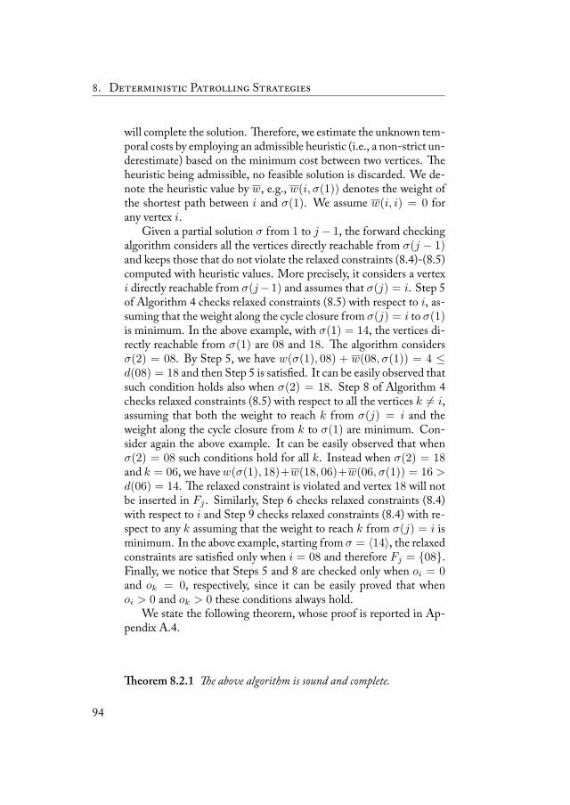
. D P S

will complete the solution. erefore, we estimate the unknown tem-poral costs by employing an admissible heuristic (i.e., a non-strict un-derestimate) based on the minimum cost between two vertices. eheuristic being admissible, no feasible solution is discarded. We de-note the heuristic value by w, e.g., w(i, σ(1)) denotes the weight ofthe shortest path between i and σ(1). We assume w(i, i) = 0 forany vertex i.

Given a partial solution σ from 1 to j − 1, the forward checkingalgorithm considers all the vertices directly reachable from σ(j − 1)and keeps those that do not violate the relaxed constraints (8.4)-(8.5)computed with heuristic values. More precisely, it considers a vertexi directly reachable from σ(j−1) and assumes that σ(j) = i. Step 5of Algorithm 4 checks relaxed constraints (8.5) with respect to i, as-suming that the weight along the cycle closure from σ(j) = i to σ(1)is minimum. In the above example, with σ(1) = 14, the vertices di-rectly reachable from σ(1) are 08 and 18. e algorithm considersσ(2) = 08. By Step 5, we have w(σ(1), 08) + w(08, σ(1)) = 4 ≤d(08) = 18 and then Step 5 is satisfied. It can be easily observed thatsuch condition holds also when σ(2) = 18. Step 8 of Algorithm 4checks relaxed constraints (8.5) with respect to all the vertices k 6= i,assuming that both the weight to reach k from σ(j) = i and theweight along the cycle closure from k to σ(1) are minimum. Con-sider again the above example. It can be easily observed that whenσ(2) = 08 such conditions hold for all k. Instead when σ(2) = 18and k = 06, we havew(σ(1), 18)+w(18, 06)+w(06, σ(1)) = 16 >d(06) = 14. e relaxed constraint is violated and vertex 18 will notbe inserted in Fj . Similarly, Step 6 checks relaxed constraints (8.4)with respect to i and Step 9 checks relaxed constraints (8.4) with re-spect to any k assuming that the weight to reach k from σ(j) = i isminimum. In the above example, starting from σ = 〈14〉, the relaxedconstraints are satisfied only when i = 08 and therefore Fj = {08}.Finally, we notice that Steps 5 and 8 are checked only when oi = 0and ok = 0, respectively, since it can be easily proved that whenoi > 0 and ok > 0 these conditions always hold.

We state the following theorem, whose proof is reported in Ap-pendix A.4.

eorem 8.2.1 e above algorithm is sound and complete.

94

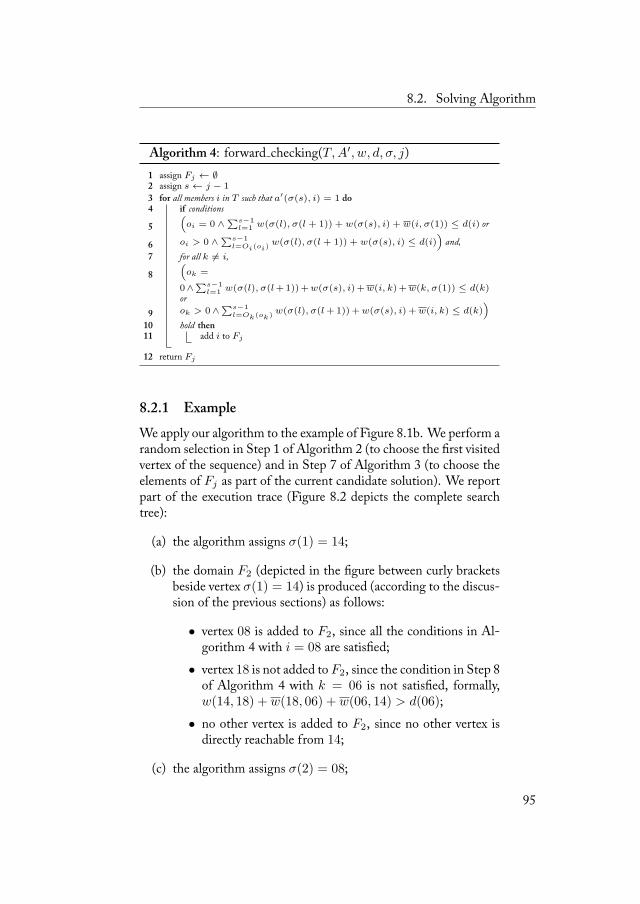
8.2. Solving Algorithm

Algorithm 4: forward checking(T,A′, w, d, σ, j)assign Fj ← ∅1assign s← j − 12for all members i in T such that a′(σ(s), i) = 1 do3

if conditions4 (oi = 0 ∧

∑s−1l=1 w(σ(l), σ(l + 1)) + w(σ(s), i) + w(i, σ(1)) ≤ d(i) or5

oi > 0 ∧∑s−1

l=Oi(oi)w(σ(l), σ(l + 1)) + w(σ(s), i) ≤ d(i)

)and,6

for all k 6= i,7 (ok =8

0∧∑s−1

l=1 w(σ(l), σ(l+1))+w(σ(s), i)+w(i, k)+w(k, σ(1)) ≤ d(k)orok > 0∧

∑s−1l=Ok(ok)

w(σ(l), σ(l+1))+w(σ(s), i) +w(i, k) ≤ d(k))

9hold then10

add i to Fj11

return Fj12

8.2.1 ExampleWe apply our algorithm to the example of Figure 8.1b. We perform arandom selection in Step 1 of Algorithm 2 (to choose the first visitedvertex of the sequence) and in Step 7 of Algorithm 3 (to choose theelements of Fj as part of the current candidate solution). We reportpart of the execution trace (Figure 8.2 depicts the complete searchtree):

(a) the algorithm assigns σ(1) = 14;

(b) the domain F2 (depicted in the figure between curly bracketsbeside vertex σ(1) = 14) is produced (according to the discus-sion of the previous sections) as follows:

• vertex 08 is added to F2, since all the conditions in Al-gorithm 4 with i = 08 are satisfied;

• vertex 18 is not added to F2, since the condition in Step 8of Algorithm 4 with k = 06 is not satisfied, formally,w(14, 18) + w(18, 06) + w(06, 14) > d(06);

• no other vertex is added to F2, since no other vertex isdirectly reachable from 14;

(c) the algorithm assigns σ(2) = 08;

95

. D P S

(d) the domain F3 is produced similarly as above, yielding to F3 ={06};

(e) the algorithm assigns σ(3) = 06 and continues.

Some issues are worth noting. In the 10th node of the search tree,a sequence σ with σ(1) = σ(s) and including all the vertices wasfound. However, this sequence does not satisfy constraints (8.5). Ifthe search is not stopped and backtracked at the the 10th node (inStep 5 of Algorithm 3), the algorithm would never terminate. In-deed, the subtrees that would follow this vertex would be the infiniterepetition of part of the tree already built. Finally, in the 6th node, nopossible successor is allowed by the forward checking, and thereforethe algorithm backtracks.

8.2.2 Improving Efficiency and Heuristics

Our algorithm can be improved as follows. Consider the conditionsin Steps 5 and 8 of Algorithm 4. Except for the first execution ofAlgorithm 4 (i.e., when j = 2), the satisfaction of the condition atStep 5 for a given j is guaranteed if the condition in Step 8 for j − 1is satisfied. erefore, we can safely limit the algorithm to check theconditions at Step 5 exclusively when j = 2. e same considerationshold also for the conditions in Steps 6 and 9. erefore, we can safelylimit the algorithm to check the conditions at Step 6 and 9 exclusivelywhen j = 2.

We can introduce a more sophisticated stopping criterion calledLSC (Length Stopping Criterion) based on eorem 8.1.5 and suchthat if

∑s−1l=1 w(σ(l), σ(l + 1)) + w(σ(s), σ(1)) > maxt∈T {d(t)},

then the search is stopped and backtracked. We can also introduce ana priori check (IFC, Initial Forward Checking): before starting thesearch, we consider each vertex as the root node of the search treeand we apply the forward checking. If at least one domain is empty,the algorithm returns failure. Otherwise, the tree search is started.

Finally, we propose some heuristic criteria for choosing from setFj the next vertex to expand in Step 8 of Algorithm 3: lexicographic(hl), random with uniform probability distribution (hr), maximumand minimum number of incident arcs (hmax a and hmin a), less vis-ited (hmin v), andmaximum andminimumpenetration time (hmax d

and hmin d). For all the ordering criteria except hr, we introduce a

96

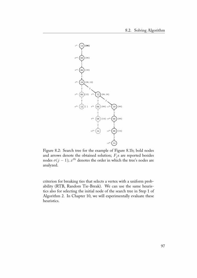
8.2. Solving Algorithm

14

08

06

18

12

06

08

14

18

06

08

14

06

12

2

25

22252

2

22

5

2

2

2

5

2

2

{08}

{06}

{18}

{06, 12}

{06, 18}

{08}

{14}

{ } {06}

{08}

{14}

{12}

{08}1st

2nd

3rd

4th

5th

6th

7th

8th

9th

10th

11th

12th

13th

14th

Figure 8.2: Search tree for the example of Figure 8.1b; bold nodesand arrows denote the obtained solution; Fjs are reported besidesnodes σ(j − 1); xth denotes the order in which the tree's nodes areanalyzed.

criterion for breaking ties that selects a vertex with a uniform prob-ability (RTB, Random Tie-Break). We can use the same heuris-tics also for selecting the initial node of the search tree in Step 1 ofAlgorithm 2. In Chapter 10, we will experimentally evaluate theseheuristics.

97

Simplifying a Patrolling Game 9

Looking for general solutions, i.e., randomized strategies, poses sev-eral computational difficulties, especially for settings with a realis-tically large number of vertices and targets, even assuming that thestrategies are Markovian. However, in this chapter we show somegame theoretical techniques that can be applied to reduce the size ofthe game. is reduction improves the resolution efficiency, savingcomputational time. More precisely, we propose algorithms to re-move agents' dominated strategies and we discuss how to use game-theoretical abstractions to further simplify the game.

9.1 Removing Dominated Strategies

In this section we present some techniques that can be exploited tosimplify a patrolling game before solving it and that are based on theremoval of the players' dominated strategies. A strategy is dominatedwhen it assigns to a dominated action a non-null probability of beingplayed. An action a is dominated by an action b when the expectedutility of playing a is larger than that of playing b independently ofthe actions played by others. To remove dominated strategies weidentify and discard dominated actions, obtaining an equivalent (withthe same equilibria) but smaller game with a consequent reduction ofthe computational time needed for its resolution.

99

. S P G

9.1.1 Patroller's Dominated ActionsIn order to be dominated, a patroller's action move(j) has to sat-isfy the following condition: if such action is removed from the setof patroller's available actions, i.e., the patroller is prevented fromvisiting vertex j, then its expected utility does not decrease. ishappens when, after the removal of move(j), no capture probabil-ity Pc(t, i) ∀t ∈ T, i ∈ V \ {j} (i.e., for each intruder's strategy)decreases. Formally, removing move(j) means reducing graph G byremoving vertex j and all its incident arcs.

Patroller's dominated actions are identified in two steps. e firstone focuses on vertices and corresponding incident arcs and it is basedon the following theorem, whose proof is reported in Appendix A.5

eorem 9.1.1 Visiting a vertex that is not on any shortest path betweenany pair of targets is a dominated action.

When there are multiple shortest paths connecting the same pair oftargets (t1, t2), visiting each vertex of some of them can be a domi-nated action that can be identified according to the following theo-rem, whose proof is reported in Appendix A.6.

eorem 9.1.2 Given two targets t1 and t2 and two shortest pathsP =〈t1, . . . , pi . . . , t2〉 and Q = 〈t1, . . . , qi . . . , t2〉 of length L betweenthem, if for all k ∈ {2, . . . , L − 1} and t ∈ T \ {t1, t2} we havedist(pk, t) ≥ dist(qk, t), then visiting each internal vertex of P (i.e.,all pi excluding t1 and t2) is dominated.

e first step identifies actions that are dominated independently ofthe current vertex of the patroller. Ifmove(j) is dominated, then thepatroller should not visit j from every adjacent vertex.

In the second step we account for the current vertex occupiedby the patroller by considering all the patroller's actions move(j),given that the current vertex is i. We can state the following theorem,whose proof is reported in Appendix A.7:

eorem 9.1.3 Given that the patroller is in vertex j ∈ V \ T , eachaction prescribing to remain in the same vertex j for a further turn is adominated action.

e application of eorem 9.1.3 allows us to remove all the loops ofG \ T . No more patroller's strategies can be removed independently

100

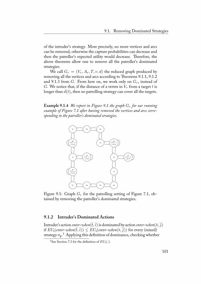
9.1. Removing Dominated Strategies

of the intruder's strategy. More precisely, no more vertices and arcscan be removed, otherwise the capture probabilities can decrease andthen the patroller's expected utility would decrease. erefore, theabove theorems allow one to remove all the patroller's dominatedstrategies.

We call Gr = (Vr, Ar, T, v, d) the reduced graph produced byremoving all the vertices and arcs according to eorems 9.1.1, 9.1.2and 9.1.3 from G. From here on, we work only on Gr, instead ofG. We notice that, if the distance of a vertex in Vr from a target t islonger than d(t), then no patrolling strategy can cover all the targets.

Example 9.1.4 We report in Figure 9.1 the graph Gr for our runningexample of Figure 7.1 after having removed the vertices and arcs corre-sponding to the patroller's dominated strategies.

01 02 03

06d(06) = 9

(.1,.6)07

08d(08) = 8

(.3,.8)

11

12d(12) = 9

(.1,.2)13

14d(14) = 9

(.2,.7)

18d(18) = 8

(.3,.6)19

21 22 23 24

Figure 9.1: Graph Gr for the patrolling setting of Figure 7.1, ob-tained by removing the patroller's dominated strategies.

9.1.2 Intruder's Dominated ActionsIntruder's action enter-when(t, i) is dominated by action enter-when(s, j)if EUi(enter-when(t, i)) ≤ EUi(enter-when(s, j)) for every (mixed)strategyσp.1 Applying this definition of dominance, checkingwhether

1See Section 7.3 for the definition of EUi(·).

101

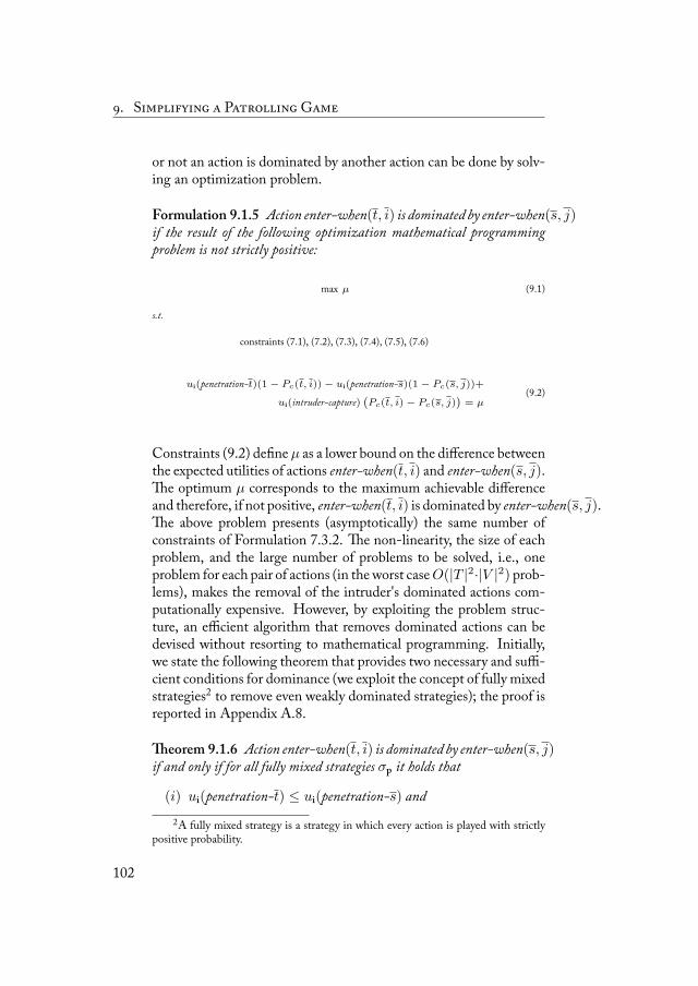
. S P G

or not an action is dominated by another action can be done by solv-ing an optimization problem.

Formulation 9.1.5 Action enter-when(t, i) is dominated by enter-when(s, j)if the result of the following optimization mathematical programmingproblem is not strictly positive:

max µ (9.1)

s.t.

constraints (7.1), (7.2), (7.3), (7.4), (7.5), (7.6)

ui(penetration-t)(1− Pc(t, i))− ui(penetration-s)(1− Pc(s, j))+

ui(intruder-capture)(Pc(t, i)− Pc(s, j)

)= µ

(9.2)

Constraints (9.2) define µ as a lower bound on the difference betweenthe expected utilities of actions enter-when(t, i) and enter-when(s, j).e optimum µ corresponds to the maximum achievable differenceand therefore, if not positive, enter-when(t, i) is dominated by enter-when(s, j).e above problem presents (asymptotically) the same number ofconstraints of Formulation 7.3.2. e non-linearity, the size of eachproblem, and the large number of problems to be solved, i.e., oneproblem for each pair of actions (in the worst caseO(|T |2·|V |2) prob-lems), makes the removal of the intruder's dominated actions com-putationally expensive. However, by exploiting the problem struc-ture, an efficient algorithm that removes dominated actions can bedevised without resorting to mathematical programming. Initially,we state the following theorem that provides two necessary and suffi-cient conditions for dominance (we exploit the concept of fully mixedstrategies2 to remove even weakly dominated strategies); the proof isreported in Appendix A.8.

eorem 9.1.6 Action enter-when(t, i) is dominated by enter-when(s, j)if and only if for all fully mixed strategies σp it holds that

(i) ui(penetration-t) ≤ ui(penetration-s) and2A fully mixed strategy is a strategy in which every action is played with strictly

positive probability.

102

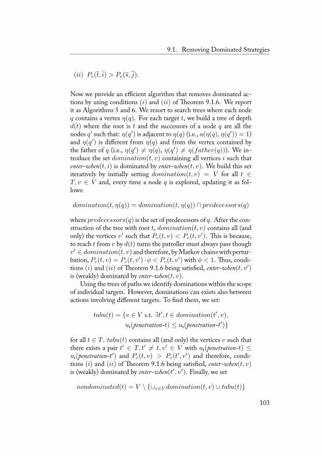
9.1. Removing Dominated Strategies

(ii) Pc(t, i) > Pc(s, j).

Now we provide an efficient algorithm that removes dominated ac-tions by using conditions (i) and (ii) of eorem 9.1.6. We reportit as Algorithms 5 and 6. We resort to search trees where each nodeq contains a vertex η(q). For each target t, we build a tree of depthd(t) where the root is t and the successors of a node q are all thenodes q′ such that: η(q′) is adjacent to η(q) (i.e., a(η(q), η(q′)) = 1)and η(q′) is different from η(q) and from the vertex contained bythe father of q (i.e., η(q′) 6= η(q), η(q′) 6= η(father(q))). We in-troduce the set domination(t, v) containing all vertices i such thatenter-when(t, i) is dominated by enter-when(t, v). We build this setiteratively by initially setting domination(t, v) = V for all t ∈T, v ∈ V and, every time a node q is explored, updating it as fol-lows:

domination(t, η(q)) = domination(t, η(q)) ∩ predecessors(q)

where predecessors(q) is the set of predecessors of q. After the con-struction of the tree with root t, domination(t, v) contains all (andonly) the vertices v′ such that Pc(t, v) < Pc(t, v

′). is is because,to reach t from v by d(t) turns the patroller must always pass thoughv′ ∈ domination(t, v) and therefore, byMarkov chains with pertur-bation, Pc(t, v) = Pc(t, v

′) ·φ < Pc(t, v′) with φ < 1. us, condi-

tions (i) and (ii) of eorem 9.1.6 being satisfied, enter-when(t, v′)is (weakly) dominated by enter-when(t, v).

Using the trees of paths we identify dominations within the scopeof individual targets. However, dominations can exists also betweenactions involving different targets. To find them, we set:

tabu(t) = {v ∈ V s.t. ∃t′, t ∈ domination(t′, v),

ui(penetration-t) ≤ ui(penetration-t′)}

for all t ∈ T . tabu(t) contains all (and only) the vertices v such thatthere exists a pair t′ ∈ T, t′ 6= t, v′ ∈ V with ui(penetration-t) ≤ui(penetration-t′) and Pc(t, v) > Pc(t

′, v′) and therefore, condi-tions (i) and (ii) of eorem 9.1.6 being satisfied, enter-when(t, v)is (weakly) dominated by enter-when(t′, v′). Finally, we set

nondominated(t) = V \ {∪v∈V domination(t, v) ∪ tabu(t)}

103

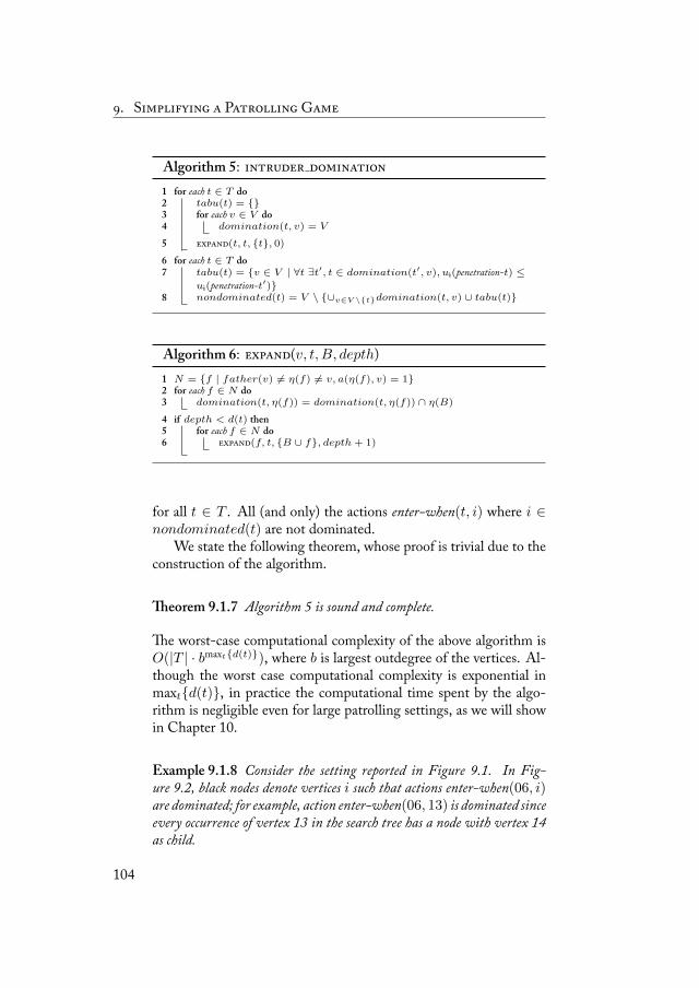
. S P G

Algorithm 5: for each t ∈ T do1

tabu(t) = {}2for each v ∈ V do3

domination(t, v) = V4(t, t, {t}, 0)5

for each t ∈ T do6tabu(t) = {v ∈ V | ∀t ∃t′, t ∈ domination(t′, v), ui(penetration-t) ≤7ui(penetration-t′)}nondominated(t) = V \ {∪v∈V \{t}domination(t, v) ∪ tabu(t)}8

Algorithm 6: (v, t, B, depth)N = {f | father(v) 6= η(f) 6= v, a(η(f), v) = 1}1for each f ∈ N do2

domination(t, η(f)) = domination(t, η(f)) ∩ η(B)3if depth < d(t) then4

for each f ∈ N do5(f, t, {B ∪ f}, depth + 1)6

for all t ∈ T . All (and only) the actions enter-when(t, i) where i ∈nondominated(t) are not dominated.

We state the following theorem, whose proof is trivial due to theconstruction of the algorithm.

eorem 9.1.7 Algorithm 5 is sound and complete.

e worst-case computational complexity of the above algorithm isO(|T | · bmaxt{d(t)}), where b is largest outdegree of the vertices. Al-though the worst case computational complexity is exponential inmaxt{d(t)}, in practice the computational time spent by the algo-rithm is negligible even for large patrolling settings, as we will showin Chapter 10.

Example 9.1.8 Consider the setting reported in Figure 9.1. In Fig-ure 9.2, black nodes denote vertices i such that actions enter-when(06, i)are dominated; for example, action enter-when(06, 13) is dominated sinceevery occurrence of vertex 13 in the search tree has a node with vertex 14as child.

104

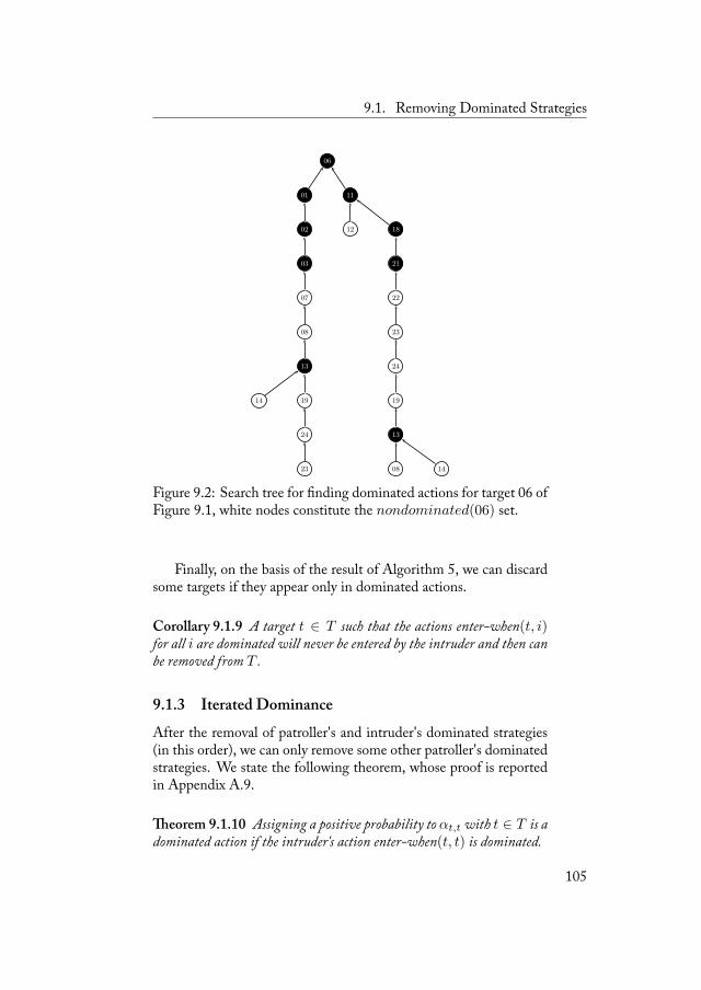
9.1. Removing Dominated Strategies

06

01 11

02 12 18

03 21

07 22

08 23

13 24

14 19 19

24 13

23 08 14

Figure 9.2: Search tree for finding dominated actions for target 06 ofFigure 9.1, white nodes constitute the nondominated(06) set.

Finally, on the basis of the result of Algorithm 5, we can discardsome targets if they appear only in dominated actions.

Corollary 9.1.9 A target t ∈ T such that the actions enter-when(t, i)for all i are dominated will never be entered by the intruder and then canbe removed from T .

9.1.3 Iterated Dominance

After the removal of patroller's and intruder's dominated strategies(in this order), we can only remove some other patroller's dominatedstrategies. We state the following theorem, whose proof is reportedin Appendix A.9.

eorem 9.1.10 Assigning a positive probability to αt,t with t ∈ T is adominated action if the intruder's action enter-when(t, t) is dominated.

105

. S P G

No more steps of iterated dominance are possible because, after theremoval of the arcs prescribed byeorem 9.1.10, the intruder's dom-inated strategies do not change.3

We remark that, by resorting to the concept of never best re-sponse [88], additional intruder's actions can be removed. However,differently from what happens for removal of dominated actions, toremove never best responses we cannot avoid using non-linear math-ematical programming. As a result, removing a never best responserequires the same computational effort as solving an instance of For-mulation 7.3.4.

9.2 Information Lossless Abstractions

Although the removal of dominated strategies drastically reduces thesize of patrolling games in terms of vertices and number of intruder'sbest responses, hence reducing the computational time of about 95%in average, the resolution of realistic games is still hard (as we showin Chapter 10). An effective technique that has received a lot ofattention in the literature to deal with large games is strategy abstrac-tion [44, 45]. In this section, we apply it to the patrolling games weare considering.

9.2.1 Abstraction Definition

e basic idea behind abstractions is to group together multiple ac-tions into a single macro action. is allows one to reduce the size ofthe game. e most interesting kind of abstractions are those with-out loss of information, allowing one to find the optimal solution ofa game by solving the abstracted one. A number of works on abstrac-tions have been developed for extensive-form games with imperfect-information and, in particular, for poker games [44, 45]. However,the application of the seminal result in [44] to patrolling games pro-duces a game that is exactly the same of the original one, patrollinggames being general-sum and without chance moves. is pushes usto define ad hoc abstractions for patrolling games.

3We notice that, after the removal of intruder's dominated actions, we can dis-cover that some targets will never be entered by the intruder. However, in our case,these targets are on some shortest paths connecting other targets and therefore theycannot be removed.

106

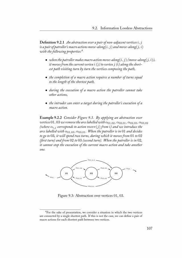
9.2. Information Lossless Abstractions

Definition 9.2.1 An abstraction over a pair of non-adjacent vertices i, jis a pair of patroller's macro actionsmove-along(i, j) andmove-along(j, i)with the following properties:4

• when the patrollermakesmacro actionmove-along(i, j) (move-along(j, i)),it moves from the current vertex i (j) to vertex j (i) along the short-est path visiting turn by turn the vertices composing the path,

• the completion of a macro action requires a number of turns equalto the length of the shortest path,

• during the execution of a macro action the patroller cannot takeother actions,

• the intruder can enter a target during the patroller's execution of amacro action.

Example 9.2.2 Consider Figure 9.3. By applying an abstraction oververtices 01, 03we remove the arcs labelledwithα01,02, α02,01, α02,03, α03,02

(where αi,j corresponds to actionmove(j) from i) and we introduce thearcs labelled with α01,03, α03,01. When the patroller is in 01 and decidesto go to 03, it will spend two turns, during which it moves from 01 to 02(first turn) and from 02 to 03 (second turn). When the patroller is in 02,it cannot stop the execution of the current macro action and take anotherone.

01 02 03

α01, ·

α01,0,3

α01,02

α02,01

α02,03

α03,02

α03,01

α03, ·

Figure 9.3: Abstraction over vertices 01, 03.

4For the sake of presentation, we consider a situation in which the two verticesare connected by a single shortest path. If this is not the case, we can define a pair ofmacro actions for each shortest path between two vertices.

107

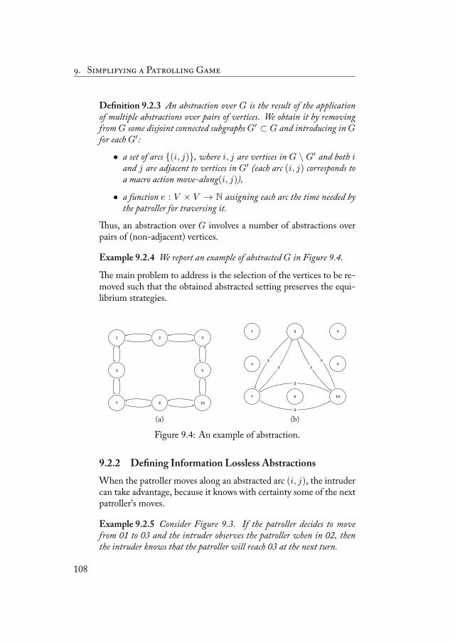
. S P G

Definition 9.2.3 An abstraction over G is the result of the applicationof multiple abstractions over pairs of vertices. We obtain it by removingfromG some disjoint connected subgraphsG′ ⊂ G and introducing inGfor eachG′:

• a set of arcs {(i, j)}, where i, j are vertices in G \ G′ and both iand j are adjacent to vertices in G′ (each arc (i, j) corresponds toa macro action move-along(i, j)),

• a function e : V × V → N assigning each arc the time needed bythe patroller for traversing it.

us, an abstraction over G involves a number of abstractions overpairs of (non-adjacent) vertices.

Example 9.2.4 We report an example of abstractedG in Figure 9.4.

e main problem to address is the selection of the vertices to be re-moved such that the obtained abstracted setting preserves the equi-librium strategies.

1 2 3

4 5

7 8 10

(a)

1 2 3

4 5

7 8 10

3

33

3

2

2

(b)

Figure 9.4: An example of abstraction.

9.2.2 Defining Information Lossless AbstractionsWhen the patroller moves along an abstracted arc (i, j), the intrudercan take advantage, because it knows with certainty some of the nextpatroller's moves.

Example 9.2.5 Consider Figure 9.3. If the patroller decides to movefrom 01 to 03 and the intruder observes the patroller when in 02, thenthe intruder knows that the patroller will reach 03 at the next turn.

108

9.2. Information Lossless Abstractions

We produce information lossless abstractions such that the set of in-truder's dominated strategies (computed as discussed in Section 9.1.2)is an invariant, namely they are left unchanged by the application ofabstractions. As a result, the intruder will never (optimally) enter atarget during the patroller's execution of an action move-along(i, j)and therefore it cannot take advantage from knowing some of thenext patroller's moves. We state the following theorem, whose proofis trivial and then omitted.

eorem 9.2.6 A necessary condition for an (ex-ante) abstraction to bewithout information loss is that the set of intruder's dominated strategiesis invariant.

We provide some necessary conditions for a vertex to be removedduring the application of an abstraction without changing the set ofintruder's dominated strategies.

Corollary 9.2.7 e removal of a vertex i during the application of anabstraction can be without information loss only if:

• when i 6∈ T , for all t ∈ T , actions enter-when(t, i) are dominated,

• when i ∈ T , for all t ∈ T , actions enter-when(t, i) are dominatedand, for all j ∈ V , actions enter-when(i, j) are dominated.

Assuring that the set of intruder's dominated strategies does not changeis not sufficient, because we need to assure that solving the abstractedgame we can find a strategy no worse than the optimal strategy inthe non-abstracted game. We denote by dom(i, t) the set of ver-tices i′ such that enter-when(t, i′) is not dominated and dominatesenter-when(t, i) (as calculated in Section 9.1.2). We state the fol-lowing theorem, whose proof is reported in Appendix A.10.

eorem 9.2.8 Given an abstraction over G, if, for all the abstractionsover pairs of vertices i, j and for all vertices k on the shortest path con-necting i and j:

• dist(i, dom(k, t)) ≥ dist(i, k) and

• dist(j, dom(k, t)) ≥ dist(j, k) for all targets t ∈ T ,

109

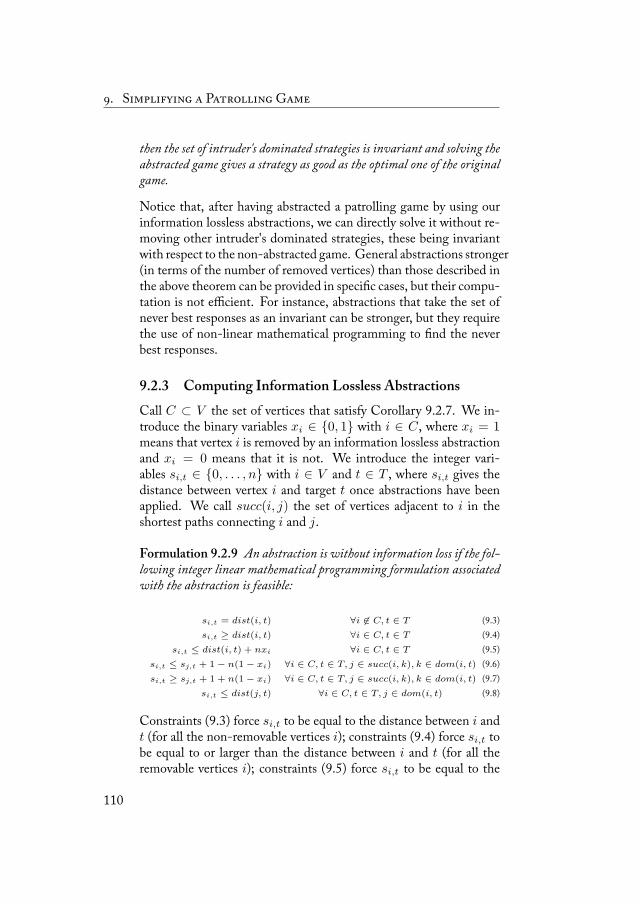
. S P G

then the set of intruder's dominated strategies is invariant and solving theabstracted game gives a strategy as good as the optimal one of the originalgame.

Notice that, after having abstracted a patrolling game by using ourinformation lossless abstractions, we can directly solve it without re-moving other intruder's dominated strategies, these being invariantwith respect to the non-abstracted game. General abstractions stronger(in terms of the number of removed vertices) than those described inthe above theorem can be provided in specific cases, but their compu-tation is not efficient. For instance, abstractions that take the set ofnever best responses as an invariant can be stronger, but they requirethe use of non-linear mathematical programming to find the neverbest responses.

9.2.3 Computing Information Lossless AbstractionsCall C ⊂ V the set of vertices that satisfy Corollary 9.2.7. We in-troduce the binary variables xi ∈ {0, 1} with i ∈ C, where xi = 1means that vertex i is removed by an information lossless abstractionand xi = 0 means that it is not. We introduce the integer vari-ables si,t ∈ {0, . . . , n} with i ∈ V and t ∈ T , where si,t gives thedistance between vertex i and target t once abstractions have beenapplied. We call succ(i, j) the set of vertices adjacent to i in theshortest paths connecting i and j.

Formulation 9.2.9 An abstraction is without information loss if the fol-lowing integer linear mathematical programming formulation associatedwith the abstraction is feasible:

si,t = dist(i, t) ∀i 6∈ C, t ∈ T (9.3)si,t ≥ dist(i, t) ∀i ∈ C, t ∈ T (9.4)

si,t ≤ dist(i, t) + nxi ∀i ∈ C, t ∈ T (9.5)si,t ≤ sj,t + 1− n(1− xi) ∀i ∈ C, t ∈ T, j ∈ succ(i, k), k ∈ dom(i, t) (9.6)si,t ≥ sj,t + 1 + n(1− xi) ∀i ∈ C, t ∈ T, j ∈ succ(i, k), k ∈ dom(i, t) (9.7)

si,t ≤ dist(j, t) ∀i ∈ C, t ∈ T, j ∈ dom(i, t) (9.8)

Constraints (9.3) force si,t to be equal to the distance between i andt (for all the non-removable vertices i); constraints (9.4) force si,t tobe equal to or larger than the distance between i and t (for all theremovable vertices i); constraints (9.5) force si,t to be equal to the

110

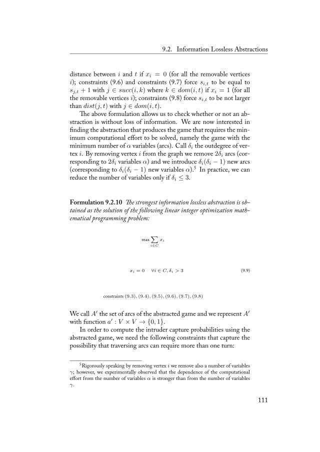
9.2. Information Lossless Abstractions

distance between i and t if xi = 0 (for all the removable verticesi); constraints (9.6) and constraints (9.7) force si,t to be equal tosj,t + 1 with j ∈ succ(i, k) where k ∈ dom(i, t) if xi = 1 (for allthe removable vertices i); constraints (9.8) force si,t to be not largerthan dist(j, t) with j ∈ dom(i, t).

e above formulation allows us to check whether or not an ab-straction is without loss of information. We are now interested infinding the abstraction that produces the game that requires the min-imum computational effort to be solved, namely the game with theminimum number of α variables (arcs). Call δi the outdegree of ver-tex i. By removing vertex i from the graph we remove 2δi arcs (cor-responding to 2δi variables α) and we introduce δi(δi − 1) new arcs(corresponding to δi(δi − 1) new variables α).5 In practice, we canreduce the number of variables only if δi ≤ 3.

Formulation 9.2.10 e strongest information lossless abstraction is ob-tained as the solution of the following linear integer optimization math-ematical programming problem:

max∑i∈C

xi

xi = 0 ∀i ∈ C, δi > 3 (9.9)

constraints (9.3), (9.4), (9.5), (9.6), (9.7), (9.8)

We call A′ the set of arcs of the abstracted game and we represent A′with function a′ : V × V → {0, 1}.

In order to compute the intruder capture probabilities using theabstracted game, we need the following constraints that capture thepossibility that traversing arcs can require more than one turn:

5Rigorously speaking by removing vertex i we remove also a number of variablesγ; however, we experimentally observed that the dependence of the computationaleffort from the number of variables α is stronger than from the number of variablesγ.

111

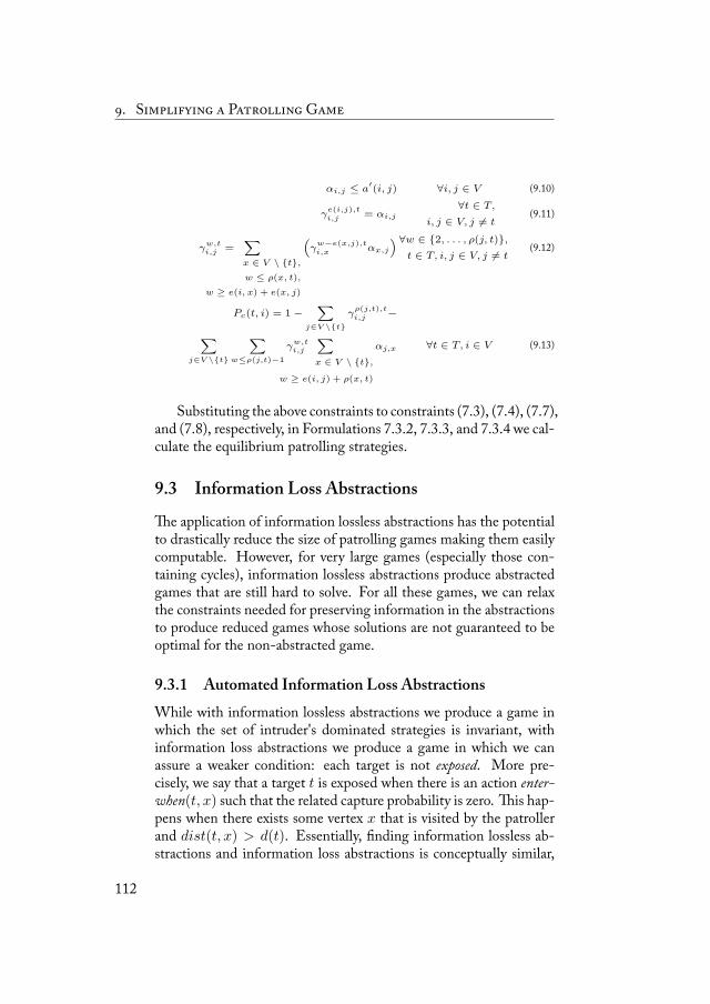
. S P G

αi,j ≤ a′(i, j) ∀i, j ∈ V (9.10)

γe(i,j),ti,j = αi,j

∀t ∈ T,

i, j ∈ V, j 6= t(9.11)

γw,ti,j =

∑x ∈ V \ {t},w ≤ ρ(x, t),

w ≥ e(i, x) + e(x, j)

(γw−e(x,j),ti,x αx,j

) ∀w ∈ {2, . . . , ρ(j, t)},t ∈ T, i, j ∈ V, j 6= t

(9.12)

Pc(t, i) = 1−∑

j∈V \{t}

γρ(j,t),ti,j −

∑j∈V \{t}

∑w≤ρ(j,t)−1

γw,ti,j

∑x ∈ V \ {t},

w ≥ e(i, j) + ρ(x, t)

αj,x ∀t ∈ T, i ∈ V (9.13)

Substituting the above constraints to constraints (7.3), (7.4), (7.7),and (7.8), respectively, in Formulations 7.3.2, 7.3.3, and 7.3.4 we cal-culate the equilibrium patrolling strategies.

9.3 Information Loss Abstractions

e application of information lossless abstractions has the potentialto drastically reduce the size of patrolling games making them easilycomputable. However, for very large games (especially those con-taining cycles), information lossless abstractions produce abstractedgames that are still hard to solve. For all these games, we can relaxthe constraints needed for preserving information in the abstractionsto produce reduced games whose solutions are not guaranteed to beoptimal for the non-abstracted game.

9.3.1 Automated Information Loss AbstractionsWhile with information lossless abstractions we produce a game inwhich the set of intruder's dominated strategies is invariant, withinformation loss abstractions we produce a game in which we canassure a weaker condition: each target is not exposed. More pre-cisely, we say that a target t is exposed when there is an action enter-when(t, x) such that the related capture probability is zero. is hap-pens when there exists some vertex x that is visited by the patrollerand dist(t, x) > d(t). Essentially, finding information lossless ab-stractions and information loss abstractions is conceptually similar,

112

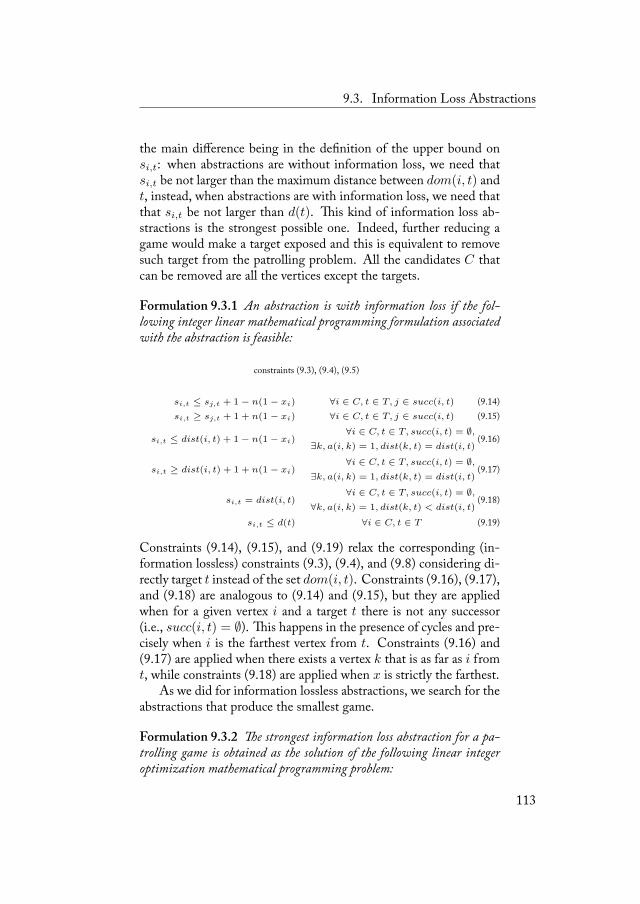
9.3. Information Loss Abstractions

the main difference being in the definition of the upper bound onsi,t: when abstractions are without information loss, we need thatsi,t be not larger than the maximum distance between dom(i, t) andt, instead, when abstractions are with information loss, we need thatthat si,t be not larger than d(t). is kind of information loss ab-stractions is the strongest possible one. Indeed, further reducing agame would make a target exposed and this is equivalent to removesuch target from the patrolling problem. All the candidates C thatcan be removed are all the vertices except the targets.

Formulation 9.3.1 An abstraction is with information loss if the fol-lowing integer linear mathematical programming formulation associatedwith the abstraction is feasible:

constraints (9.3), (9.4), (9.5)

si,t ≤ sj,t + 1− n(1− xi) ∀i ∈ C, t ∈ T, j ∈ succ(i, t) (9.14)si,t ≥ sj,t + 1 + n(1− xi) ∀i ∈ C, t ∈ T, j ∈ succ(i, t) (9.15)

si,t ≤ dist(i, t) + 1− n(1− xi)∀i ∈ C, t ∈ T, succ(i, t) = ∅,

∃k, a(i, k) = 1, dist(k, t) = dist(i, t)(9.16)

si,t ≥ dist(i, t) + 1 + n(1− xi)∀i ∈ C, t ∈ T, succ(i, t) = ∅,

∃k, a(i, k) = 1, dist(k, t) = dist(i, t)(9.17)

si,t = dist(i, t)∀i ∈ C, t ∈ T, succ(i, t) = ∅,

∀k, a(i, k) = 1, dist(k, t) < dist(i, t)(9.18)

si,t ≤ d(t) ∀i ∈ C, t ∈ T (9.19)

Constraints (9.14), (9.15), and (9.19) relax the corresponding (in-formation lossless) constraints (9.3), (9.4), and (9.8) considering di-rectly target t instead of the set dom(i, t). Constraints (9.16), (9.17),and (9.18) are analogous to (9.14) and (9.15), but they are appliedwhen for a given vertex i and a target t there is not any successor(i.e., succ(i, t) = ∅). is happens in the presence of cycles and pre-cisely when i is the farthest vertex from t. Constraints (9.16) and(9.17) are applied when there exists a vertex k that is as far as i fromt, while constraints (9.18) are applied when x is strictly the farthest.

As we did for information lossless abstractions, we search for theabstractions that produce the smallest game.

Formulation 9.3.2 e strongest information loss abstraction for a pa-trolling game is obtained as the solution of the following linear integeroptimization mathematical programming problem:

113

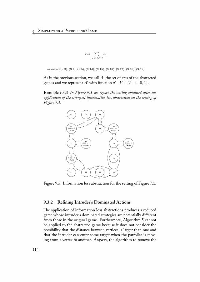
. S P G

max∑

i∈C,δi≤3

xi

constraints (9.3), (9.4), (9.5), (9.14), (9.15), (9.16), (9.17), (9.18), (9.19)

As in the previous section, we call A′ the set of arcs of the abstractedgames and we represent A′ with function a′ : V × V → {0, 1}.

Example 9.3.3 In Figure 9.5 we report the setting obtained after theapplication of the strongest information loss abstraction on the setting ofFigure 7.1.

01 02 03

06d(06) = 9

(.1,.6)07

08d(08) = 8

(.3,.8)

11

12d(12) = 9

(.1,.2)13

14d(14) = 9

(.2,.7)

18d(18) = 8

(.3,.6)19

21 22 23 24

3

3

2

2

2

2

22

Figure 9.5: Information loss abstraction for the setting of Figure 7.1.

9.3.2 Refining Intruder's Dominated Actionse application of information loss abstractions produces a reducedgame whose intruder's dominated strategies are potentially differentfrom those in the original game. Furthermore, Algorithm 5 cannotbe applied to the abstracted game because it does not consider thepossibility that the distance between vertices is larger than one andthat the intruder can enter some target when the patroller is mov-ing from a vertex to another. Anyway, the algorithm to remove the

114

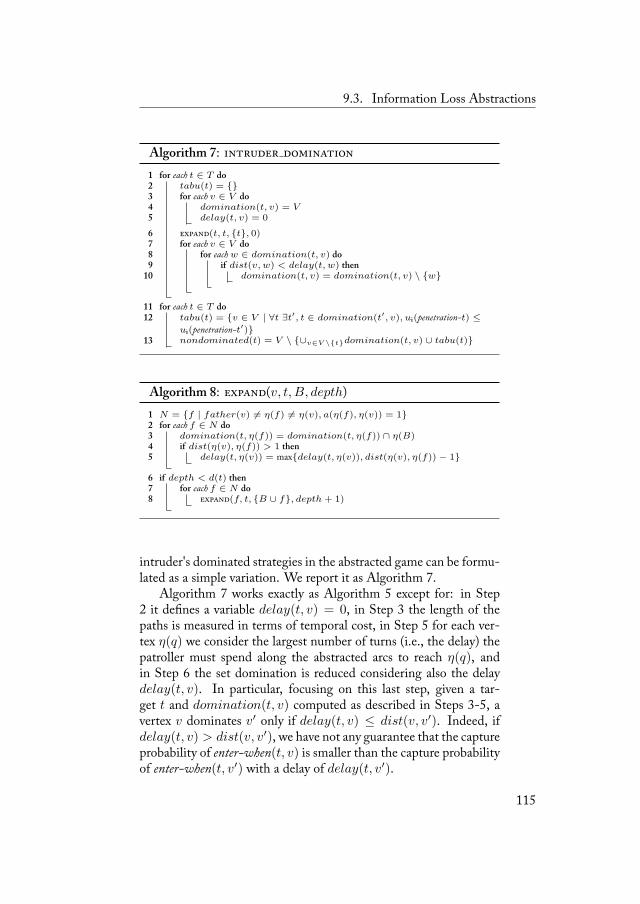
9.3. Information Loss Abstractions

Algorithm 7: for each t ∈ T do1

tabu(t) = {}2for each v ∈ V do3

domination(t, v) = V4delay(t, v) = 05

(t, t, {t}, 0)6for each v ∈ V do7

for eachw ∈ domination(t, v) do8if dist(v, w) < delay(t, w) then9

domination(t, v) = domination(t, v) \ {w}10

for each t ∈ T do11tabu(t) = {v ∈ V | ∀t ∃t′, t ∈ domination(t′, v), ui(penetration-t) ≤12ui(penetration-t′)}nondominated(t) = V \ {∪v∈V \{t}domination(t, v) ∪ tabu(t)}13

Algorithm 8: (v, t, B, depth)N = {f | father(v) 6= η(f) 6= η(v), a(η(f), η(v)) = 1}1for each f ∈ N do2

domination(t, η(f)) = domination(t, η(f)) ∩ η(B)3if dist(η(v), η(f)) > 1 then4

delay(t, η(v)) = max{delay(t, η(v)), dist(η(v), η(f))− 1}5

if depth < d(t) then6for each f ∈ N do7

(f, t, {B ∪ f}, depth + 1)8

intruder's dominated strategies in the abstracted game can be formu-lated as a simple variation. We report it as Algorithm 7.

Algorithm 7 works exactly as Algorithm 5 except for: in Step2 it defines a variable delay(t, v) = 0, in Step 3 the length of thepaths is measured in terms of temporal cost, in Step 5 for each ver-tex η(q) we consider the largest number of turns (i.e., the delay) thepatroller must spend along the abstracted arcs to reach η(q), andin Step 6 the set domination is reduced considering also the delaydelay(t, v). In particular, focusing on this last step, given a tar-get t and domination(t, v) computed as described in Steps 3-5, avertex v dominates v′ only if delay(t, v) ≤ dist(v, v′). Indeed, ifdelay(t, v) > dist(v, v′), we have not any guarantee that the captureprobability of enter-when(t, v) is smaller than the capture probabilityof enter-when(t, v′) with a delay of delay(t, v′).

115

. S P G

Once we have removed intruder's dominated strategies, the com-putation of the leader-follower equilibrium is based on the samemath-ematical programming formulation used for information lossless ab-stractions (Section 9.2.3) except that, for each non-dominated actionenter-when(t, v), we use d(t)− delay(t, v) instead of delay(t, v).

116

Experimental Evaluation 10

Exploiting the problem's structure to find a deterministic strategy(Chapter 8) and to simplify the game (Chapter 9) enables the compu-tation of equilibrium patrolling strategies for large patrolling settings,typically involving some dozens of vertices and targets (e.g., see [67]).In this chapter, we aim at obtaining experimental insights on the sizeof instances that can be tackled with reasonable computational re-sources. e two approaches presented in the previous chapters arebased on resolution techniques with different computational prop-erties whose experimental evaluation requires distinct data sets andanalyses. For this reason, following the same scheme of their presen-tation, we discuss the corresponding experimental results separately.Moreover, we provide a comparison by showing the computationaladvantages of finding a deterministic strategy (when it exists) withrespect to the algorithm for randomized strategies. Finally, we movetoward the implementation of our approach, addressing a number ofissues involved in applying our patrolling strategies in a realistic robotcontroller. We verify if the optimal patrolling strategy performs wellalso in situations that violate the idealized assumptions of the the-oretical model and we assess how much it outperforms other (non-optimal) patrolling strategies that require much less computationaleffort for their development.

117

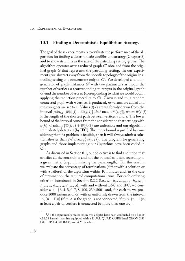
. E E

10.1 Finding a Deterministic Equilibrium Strategy

egoal of these experiments is to evaluate the performance of the al-gorithm for finding a deterministic equilibrium strategy (Chapter 8)and to show its limits as the size of the patrolling setting grows. ealgorithm operates over a reduced graph G′ obtained from the orig-inal graph G that represents the patrolling setting. In our experi-ments, we abstract away from the specific topology of the original pa-trolling setting and concentrate only on G′. We developed a randomgenerator of graph instances G′ with two parameters as input: thenumber of vertices n (corresponding to targets in the original graphG) and the number of arcsm (corresponding to what wewould obtainapplying the reduction procedure to G). Given n and m, a randomconnected graphwithn vertices is produced,m−n arcs are added andtheir weights are set to 1. Values d(k) are uniformly drawn from theinterval [mini,j {w(i, j) + w(j, i)}, 2n2 maxi,j w(i, j)], wherew(i, j)is the length of the shortest path between vertices i and j. e lowerbound of the interval comes from the consideration that settings withd(k) < mini,j {w(i, j) + w(j, i)} are unfeasible and our algorithmimmediately detects it (by IFC). e upper bound is justified by con-sidering that if a problem is feasible, then it will always admit a solu-tion shorter than 2n2 maxi,j{w(i, j)}. e program for generatinggraphs and those implementing our algorithms have been coded inC1.

As discussed in Section 8.1, our objective is to find a solution thatsatisfies all the constraints and not the optimal solution according toa given metric (e.g., minimizing the cycle length). For this reason,we evaluate the percentage of terminations (either with a solution orwith a failure) of the algorithm within 10 minutes and, in the caseof termination, the required computational time. For each orderingcriterion introduced in Section 8.2.2 (i.e., hl, hr, hmax a, hmin a,hmin v, hmax d, hmin d), with and without LSC and IFC, we con-sider n ∈ {3, 4, 5, 6, 7, 8, 100, 250, 500} and, for each n, we pro-duce 1000 instances ofG′ withm uniformly drawn from the interval[n, (n− 1)n] (if m < n the graph is not connected, if m > (n− 1)nat least a pair of vertices is connected by more than one arc).

1All the experiments presented in this chapter have been conducted on a Linux(2.6.24 kernel) machine equipped with a DUAL QUAD CORE Intel XEON 2.33GHz CPU, 4 GB RAM, and 4 MB cache.

118

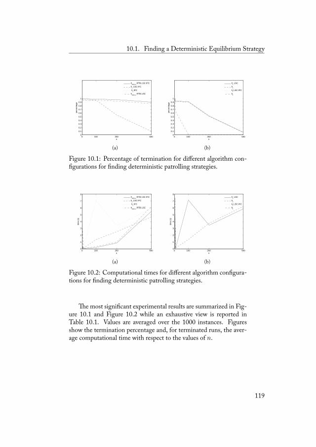
10.1. Finding a Deterministic Equilibrium Strategy

0 100 250 5000

0.1

0.2

0.3

0.4

0.5

0.6

0.7

0.8

0.9

1

n

perc

enta

ge

h

min v RTB LSC IFC

hr LSC IFC

hr IFC

hmin v

RTB LSC

(a)

0 100 250 5000

0.1

0.2

0.3

0.4

0.5

0.6

0.7

0.8

0.9

1

n

perc

enta

ge

h

r LSC

hr

hl LSC IFC

hl

(b)

Figure 10.1: Percentage of termination for different algorithm con-figurations for finding deterministic patrolling strategies.

0 100 250 5000

1

2

3

4

5

6

7

8

n

time

(s)

h

min v RTB LSC IFC

hr LSC IFC

hr IFC

hmin v

RTB LSC

(a)

0 100 250 5000

1

2

3

4

5

6

7

8

n

time

(s)

h

r LSC

hr

hl LSC IFC

hl

(b)

Figure 10.2: Computational times for different algorithm configura-tions for finding deterministic patrolling strategies.

e most significant experimental results are summarized in Fig-ure 10.1 and Figure 10.2 while an exhaustive view is reported inTable 10.1. Values are averaged over the 1000 instances. Figuresshow the termination percentage and, for terminated runs, the aver-age computational time with respect to the values of n.

119

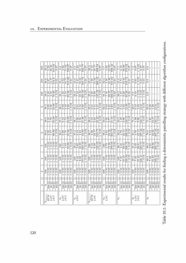
. E E

n3

45

67

8100

250

500

hm

in

v%

100

100

100

99.8

99.6

99.5

98.9

96.6

90.2

RTB

time[

s]<

0.01

<0.01

<0.01

0.32

0.10

0.05

0.16

0.87

5.50

LSC

dev[

s]<

0.01

<0.01

<0.01

5.17

1.78

0.96

3.52

14.47

30.28

IFC

max

[s]

<0.01

<0.01

<0.01

98.00

35.00

19.00

78.26

316.9

413.94

min

[s]

<0.01

<0.01

<0.01

<0.01

<0.01

<0.01

<0.01

0.01

0.07

hr

%100

100

100

98.5

97.5

96.5

95.1

55.1

9.8

LSC

time[

s]<

0.01

<0.01

0.11

0.09

0.16

0.02

1.34

2.52

4.66

IFC

dev[

s]<

0.01

<0.01

1.64

1.70

1.73

0.18

6.19

16.75

51.62

max

[s]

<0.01

<0.01

32.00

33.00

24.00

2.00

93.36

513.66

590.87

min

[s]

<0.01

<0.01

<0.01

<0.01

<0.01

<0.01

<0.01

0.01

0.07

hr

%100

100

99.0

97.2

96.7

95.5

94.0

53.0

8.9

IFC

time[

s]<

0.01

0.44

3.65

0.14

0.26

0.01

7.12

3.41

5.94

dev[

s]<

0.01

8.68

38.89

2.24

2.36

0.16

39.32

18.02

55.14

max

[s]

<0.01

173.55

594.10

43.03

31.86

2.09

561.95

501.72

582.77

min

[s]

<0.01

<0.01

<0.01

<0.01

<0.01

<0.01

<0.01

0.01

0.07

hm

in

v%

100

100

100

96.7

96.0

95.5

95.0

93.3

86.2

RTB

time[

s]<

0.01

<0.01

0.34

2.98

0.16

0.01

0.30

1.00

6.19

LSC

dev[

s]<

0.01

<0.01

6.29

33.77

2.24

0.11

6.50

15.32

35.77

max

[s]

<0.01

<0.01

125.03

519.75

42.22

2.41

145.22

366.42

498.04

min

[s]

<0.01

<0.01

<0.01

<0.01

<0.01

<0.01

<0.01

0.01

0.07

hr

%100

100

100

95.4

93.9

92.5

91.2

52.4

7.7

LSC

time[

s]<

0.01

<0.01

0.79

3.04

0.30

0.03

7.16

3.48

5.83

dev[

s]<

0.01

<0.01

13.58

24.32

2.77

0.21

39.53

18.46

55.65

max

[s]

<0.01

<0.01

270.03

303.72

41.53

2.83

566.04

531.64

596.42

min

[s]

<0.01

<0.01

<0.01

<0.01

<0.01

<0.01

0.02

0.01

0.07

hr

%100

100

98.7

94.2

93.0

91.8

90.3

51.0

7.1

time[

s]<

0.01

7.45

2.45

4.78

1.38

0.14

1.37

3.74

6.18

dev[

s]<

0.01

55.45

28.61

42.13

9.96

1.03

6.28

18.45

56.80

max

[s]

<0.01

556.92

506.72

496.84

140.31

12.86

93.26

516.72

576.52

min

[s]

<0.01

<0.01

<0.01

<0.01

<0.01

<0.01

0.02

0.01

0.07

hl

%100

99.2

91.0

81.1

75.3

69.0

3.9

2.3

1.5

LSC

time[

s]<

0.01

7.45

2.45

4.78

1.38

0.14

0.10

0.01

0.07

IFC

dev[

s]<

0.01

55.45

28.61

42.13

9.96

1.03

<0.01

<0.01

<0.01

max

[s]

<0.01

548.41

505.74

497.46

140.11

12.01

<0.01

0.01

0.07

min

[s]

<0.01

<0.01

<0.01

<0.01

<0.01

<0.01

<0.01

0.01

0.07

hl

%100

99.2

88.0

78.0

71.7

65.0

0.0

0.0

0.0

time[

s]<

0.01

7.42

2.61

5.12

1.61

0.20

−−

−de

v[s]

<0.01

55.23

28.66

42.65

10.57

1.29

−−

−m

ax[s]

<0.01

548.41

505.74

497.46

140.11

12.01

−−

−m

in[s]

<0.01

<0.01

<0.01

<0.01

<0.01

<0.01

−−

−

Tabl

e10.

1:Exp

erim

enta

lres

ults

forfi

ndin

gad

eter

min

istic

patro

lling

strat

egywi

thdi

ffere

ntalg

orith

mco

nfigu

ratio

ns.

120

10.1. Finding a Deterministic Equilibrium Strategy

For all the algorithm configurations, the average computationaltime keeps reasonably short (few seconds) even with large values ofn. On the other hand, the termination percentage varies substan-tially in different configurations. is behavior resembles that ofmany constraint programming algorithms, whose termination timeis usually either very short (when a solution is found) or the dead-line is exceeded. Moreover, the obtained results present outliers thatcan emerge by observing the maximum computational times in Ta-ble 10.1 and that cause some irregular trends on Figure 10.2. Somecases were hard to solve and required an amount of time significantlylarge (in practice, they both reduce the percentage of termination andincrease the computational time). ese hard cases represent outlierswithin the population of instances obtained with the random graphgenerator. ey are typically characterized by tangled topologies oroddly-distributed relative deadlines.

We now comment the techniques of Section 8.2.2 for improvingthe efficiency of our algorithm.

Ordering criteria e best ordering criterion seems to be hmin v

withRTB.e experimental results withhmax a, hmin a, hmax d,hmin d are very similar to those obtained with hl and thenomitted. e criterion hmin v with RTB leads the algorithmto terminate with a percentage close to hr for small values of nand about 80% larger for large values of n. Instead, hl providesvery bad performance, especially for large values of n, when thealgorithm terminates with percentages close to 0%.

LSC e improved stopping criterion allows the algorithm to in-crease the termination percentage by a value between 0% and2%, without distinguishable effects on the computational time.is improvement depends on the configuration of the algo-rithm since it affects the construction of the search tree.

IFC is criterion allows the algorithm to increase the terminationpercentage by a value between 1% and 4%, reducing the com-putational time (since the non-feasible open settings are solvedin a negligible computational time). is improvement doesnot depend on the configuration of the algorithm since it doesnot affect the search, working before it.

Hence, the best algorithm configuration appears to be hmin v withRTB, LSC, and IFC. With this configuration, the results are satis-

121

. E E

factory: the termination percentage is high also for large settings, likethose with 500 targets, and the corresponding average computationaltime, about 5.5 s, is reasonably short.

Note that our approach is not directly comparable with the otherapproaches for finding deterministic patrolling strategies reported inChapter 6 (see also Table 6.1), because we solve a feasibility prob-lem (i.e., finding a patrolling strategy that satisfies some constraints),while other approaches solve an optimization problem (i.e., findingthe best patrolling strategy according to some criteria).

10.2 Simplifying Large Games and Finding aRandomized Equilibrium Strategy

e goal of these experiments is to show the advantages, in terms ofsettings that can be solved and in terms of computational time, pro-vided by the use of the methods for simplifying patrolling games pre-sented in Chapter 9. Given the several formulations of the patrollingproblem (see Table 6.1), to the best of our knowledge the definitionof a data set for experimentation and comparison has not yet been ad-dressed. Some partial attempts of defining non-adversarial patrollingsettings can be found in [87] (used also in [71]) where the authorspropose two arbitrary topology maps with about 50/60 vertices. elack of a suitable data set for our experimental activity pushes us todevelop an ad hoc data set.

Our data set for adversarial patrolling is partitioned in two parts.e first one is composed of settings with perimetral topologies (inwhich we further distinguish open and closed topologies), while thesecond part is composed of settings with arbitrary topologies (theseare essentially constituted of a set of (mixed) open and closed topolo-gies). e settings with arbitrary topologies have been obtained bothby introducing targets in the setting presented in [87] and by produc-ing new patrolling settings inspired by environments in RADISH.2We characterize the patrolling settings with respect to two values:the number of vertices, denoted by n, and the density of targets, de-noted by δ and representing the percentage of targets over vertices(i.e., δ = |T |/n).

2RADISH is a repository containing data sets of environmental acquisitions per-formed with real robots [59].

122

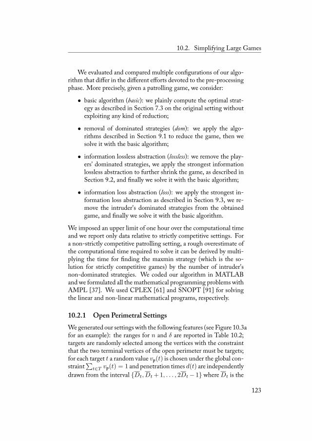
10.2. Simplifying Large Games

We evaluated and compared multiple configurations of our algo-rithm that differ in the different efforts devoted to the pre-processingphase. More precisely, given a patrolling game, we consider:

• basic algorithm (basic): we plainly compute the optimal strat-egy as described in Section 7.3 on the original setting withoutexploiting any kind of reduction;

• removal of dominated strategies (dom): we apply the algo-rithms described in Section 9.1 to reduce the game, then wesolve it with the basic algorithm;

• information lossless abstraction (lossless): we remove the play-ers' dominated strategies, we apply the strongest informationlossless abstraction to further shrink the game, as described inSection 9.2, and finally we solve it with the basic algorithm;

• information loss abstraction (loss): we apply the strongest in-formation loss abstraction as described in Section 9.3, we re-move the intruder's dominated strategies from the obtainedgame, and finally we solve it with the basic algorithm.

We imposed an upper limit of one hour over the computational timeand we report only data relative to strictly competitive settings. Fora non-strictly competitive patrolling setting, a rough overestimate ofthe computational time required to solve it can be derived by multi-plying the time for finding the maxmin strategy (which is the so-lution for strictly competitive games) by the number of intruder'snon-dominated strategies. We coded our algorithm in MATLABand we formulated all the mathematical programming problems withAMPL [37]. We used CPLEX [61] and SNOPT [91] for solvingthe linear and non-linear mathematical programs, respectively.

10.2.1 Open Perimetral SettingsWegenerated our settings with the following features (see Figure 10.3afor an example): the ranges for n and δ are reported in Table 10.2;targets are randomly selected among the vertices with the constraintthat the two terminal vertices of the open perimeter must be targets;for each target t a random value vp(t) is chosen under the global con-straint

∑t∈T vp(t) = 1 and penetration times d(t) are independently

drawn from the interval {Dt, Dt+1, . . . , 2Dt − 1} where Dt is the

123

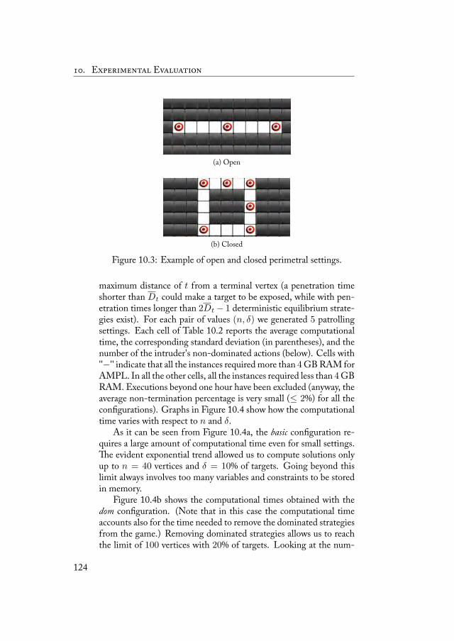
. E E

(a) Open

(b) Closed

Figure 10.3: Example of open and closed perimetral settings.

maximum distance of t from a terminal vertex (a penetration timeshorter than Dt could make a target to be exposed, while with pen-etration times longer than 2Dt − 1 deterministic equilibrium strate-gies exist). For each pair of values (n, δ) we generated 5 patrollingsettings. Each cell of Table 10.2 reports the average computationaltime, the corresponding standard deviation (in parentheses), and thenumber of the intruder's non-dominated actions (below). Cells with''−'' indicate that all the instances requiredmore than 4GBRAM forAMPL. In all the other cells, all the instances required less than 4GBRAM. Executions beyond one hour have been excluded (anyway, theaverage non-termination percentage is very small (≤ 2%) for all theconfigurations). Graphs in Figure 10.4 show how the computationaltime varies with respect to n and δ.

As it can be seen from Figure 10.4a, the basic configuration re-quires a large amount of computational time even for small settings.e evident exponential trend allowed us to compute solutions onlyup to n = 40 vertices and δ = 10% of targets. Going beyond thislimit always involves too many variables and constraints to be storedin memory.

Figure 10.4b shows the computational times obtained with thedom configuration. (Note that in this case the computational timeaccounts also for the time needed to remove the dominated strategiesfrom the game.) Removing dominated strategies allows us to reachthe limit of 100 vertices with 20% of targets. Looking at the num-

124

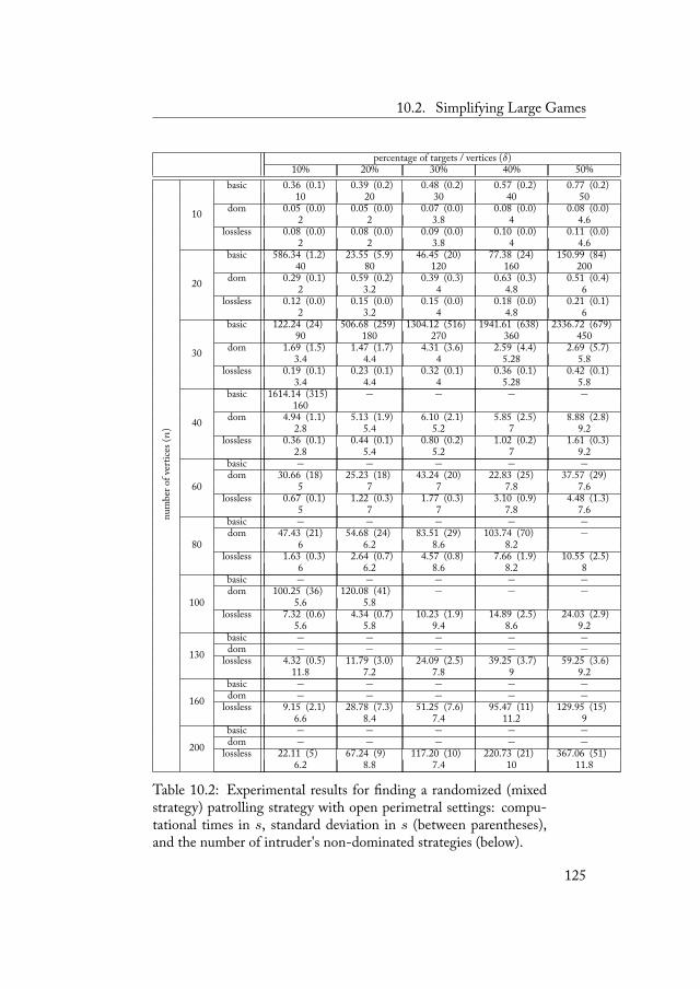
10.2. Simplifying Large Games

percentage of targets / vertices (δ)10% 20% 30% 40% 50%

num

bero

fver

tices

(n)

10

basic 0.36 (0.1) 0.39 (0.2) 0.48 (0.2) 0.57 (0.2) 0.77 (0.2)10 20 30 40 50

dom 0.05 (0.0) 0.05 (0.0) 0.07 (0.0) 0.08 (0.0) 0.08 (0.0)2 2 3.8 4 4.6

lossless 0.08 (0.0) 0.08 (0.0) 0.09 (0.0) 0.10 (0.0) 0.11 (0.0)2 2 3.8 4 4.6

20

basic 586.34 (1.2) 23.55 (5.9) 46.45 (20) 77.38 (24) 150.99 (84)40 80 120 160 200

dom 0.29 (0.1) 0.59 (0.2) 0.39 (0.3) 0.63 (0.3) 0.51 (0.4)2 3.2 4 4.8 6

lossless 0.12 (0.0) 0.15 (0.0) 0.15 (0.0) 0.18 (0.0) 0.21 (0.1)2 3.2 4 4.8 6

30

basic 122.24 (24) 506.68 (259) 1304.12 (516) 1941.61 (638) 2336.72 (679)90 180 270 360 450

dom 1.69 (1.5) 1.47 (1.7) 4.31 (3.6) 2.59 (4.4) 2.69 (5.7)3.4 4.4 4 5.28 5.8

lossless 0.19 (0.1) 0.23 (0.1) 0.32 (0.1) 0.36 (0.1) 0.42 (0.1)3.4 4.4 4 5.28 5.8

40

basic 1614.14 (315) − − − −160

dom 4.94 (1.1) 5.13 (1.9) 6.10 (2.1) 5.85 (2.5) 8.88 (2.8)2.8 5.4 5.2 7 9.2

lossless 0.36 (0.1) 0.44 (0.1) 0.80 (0.2) 1.02 (0.2) 1.61 (0.3)2.8 5.4 5.2 7 9.2

60

basic − − − − −dom 30.66 (18) 25.23 (18) 43.24 (20) 22.83 (25) 37.57 (29)

5 7 7 7.8 7.6lossless 0.67 (0.1) 1.22 (0.3) 1.77 (0.3) 3.10 (0.9) 4.48 (1.3)

5 7 7 7.8 7.6

80

basic − − − − −dom 47.43 (21) 54.68 (24) 83.51 (29) 103.74 (70) −

6 6.2 8.6 8.2lossless 1.63 (0.3) 2.64 (0.7) 4.57 (0.8) 7.66 (1.9) 10.55 (2.5)

6 6.2 8.6 8.2 8

100

basic − − − − −dom 100.25 (36) 120.08 (41) − − −

5.6 5.8lossless 7.32 (0.6) 4.34 (0.7) 10.23 (1.9) 14.89 (2.5) 24.03 (2.9)

5.6 5.8 9.4 8.6 9.2

130basic − − − − −dom − − − − −

lossless 4.32 (0.5) 11.79 (3.0) 24.09 (2.5) 39.25 (3.7) 59.25 (3.6)11.8 7.2 7.8 9 9.2

160basic − − − − −dom − − − − −

lossless 9.15 (2.1) 28.78 (7.3) 51.25 (7.6) 95.47 (11) 129.95 (15)6.6 8.4 7.4 11.2 9

200basic − − − − −dom − − − − −

lossless 22.11 (5) 67.24 (9) 117.20 (10) 220.73 (21) 367.06 (51)6.2 8.8 7.4 10 11.8

Table 10.2: Experimental results for finding a randomized (mixedstrategy) patrolling strategy with open perimetral settings: compu-tational times in s, standard deviation in s (between parentheses),and the number of intruder's non-dominated strategies (below).

125

. E E

ber of the intruder's non-dominated actions in Table 10.2 it can beobserved that the removal of dominated strategies has a remarkableimpact on the intruder's side: on average approximately 95% of in-truder's possible best responses are removed, being dominated. isshows an interesting feature of open perimetral settings: the numberof possible intruder's strategies is relatively small. Despite eliminat-ing dominated strategies obviously produces some time saving, thenumber of variables still becomes very large when n grows and theproblems are not solvable for n > 100. e percentage of the pre-processing time over the total computational time with dom is 4% onaverage (the max is 18% and the min is 1%).

e application of our information lossless abstraction removesabout 92% of the vertices. e joint reduction performed by lossless,acting both on the intruder's dominated strategies and on the numberof variables, drastically improves the efficiency of our algorithm asshown in Figure 10.4c. Enabling the lossless abstraction, settingscomposed up to 200 vertices and 50% of targets are computationallytractable. e percentage of the pre-processing time over the totalcomputational time with lossless is 76% on average (the max is 99%and the min is 9%). Given that realistic open perimetral settings(more than 200 vertices and 100 targets) are solvable with the losslessconfiguration, we did not resort to the loss configuration.

Particular closed perimetral settings with δ = 100% (namely, allvertices are targets) and with the same penetration time for all thetargets have been considered in [2]. On these settings, the com-putational time for finding the optimal patrolling strategy with themethod in [2] ismuch shorter than that corresponding to ourmethod.is is largely expected since, as discussed in Chapter 6 (see also Ta-ble 6.1), the method in [2] is specific for closed perimetral settings,while our method is applicable to more general settings.

126

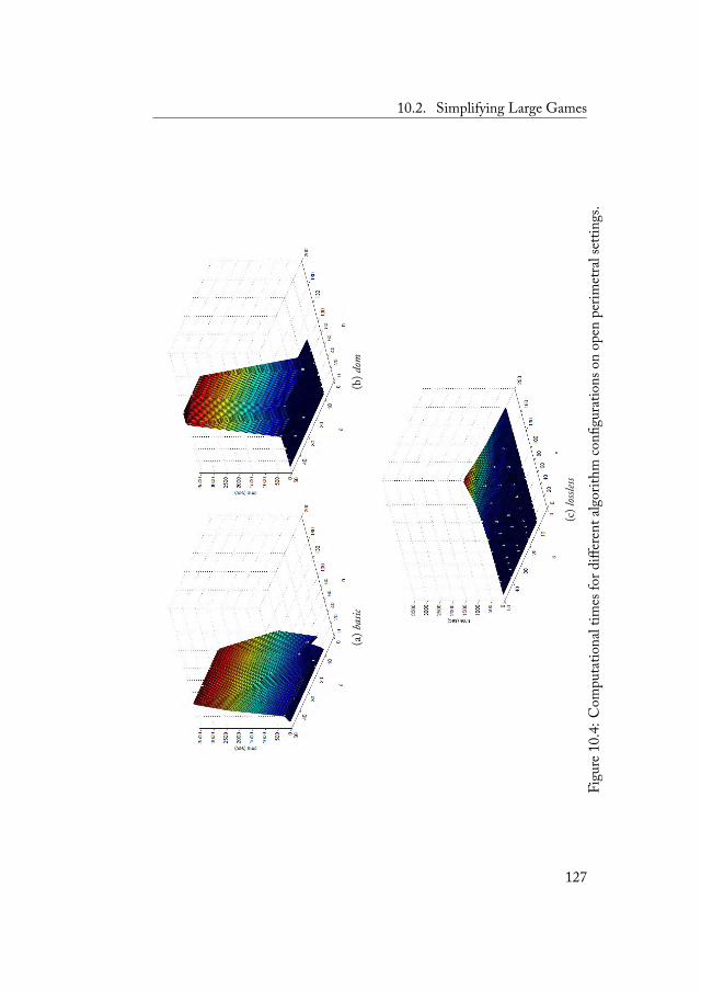
10.2. Simplifying Large Games

(a)b

asic

(b)d

om

(c)lossle

ss

Figu

re10

.4:C

ompu

tatio

nalt

imes

ford

iffer

enta

lgor

ithm

confi

gura

tions

onop

enpe

rimet

rals

ettin

gs.

127

. E E

10.2.2 Closed Perimetral Settings

Closed perimetral settings are squares with edges whose length is fvertices. We generated our settings with the following features (seeFigure 10.3b for an example): the ranges for n and δ are reportedin Table 10.3; targets are randomly selected among the vertices withthe constraints that the four corners are targets and that the graphis not reducible, by removal of patroller's dominated actions, to anopen setting; for each target t a random value vp(t) is chosen un-der the global constraint

∑t∈T vp(t) = 1 and penetration times d(t)

are independently drawn from the interval {2f, 2f + 1, . . . , n− 1}(a penetration time shorter than 2f could make a target to be ex-posed, while with penetration times longer than n− 1 deterministicequilibrium strategies exist). Table 10.3 reports the exhaustive ex-perimental results. (As for the open perimetral settings, the averagenon-termination percentage is very small, less than 2%, for all theconfigurations.)

Comparing Figure 10.4a and Figure 10.5b it can be observed thereduction of the average computational time when introducing theremoval of dominated strategies. Closed perimetral settings revealedto be more difficult with respect to open ones. Indeed, the basic con-figuration ran out of memory with n = 44 vertices and δ = 20% oftargets and only slight improvements are obtained when enabling theremoval of dominated strategies. With the dom configuration, an av-erage 41% reduction of intruder's best responses has been obtained,but the limit over the setting size is only improved to 44 vertices and30% targets. e percentage between the pre-processing time andthe total computational time with dom is < 1% on average (the maxis 2%, and the min is < 1%). We omit the results of lossless configu-ration because with closed settings no lossless abstraction is feasible.Indeed, no vertex can be removed while preserving both the set ofnon-dominated strategies and optimality; therefore the lossless con-figuration would be equivalent to the dom configuration.

e only method that can be applied at this point is to relax op-timality and compute the abstraction with information loss. Ourinformation loss abstractions remove about 72% for intruder's bestresponses. Figure 10.5c shows the obtained computational times.In this case the limit over the settings' size is n = 84 vertices withδ = 30% targets. e percentage between the pre-processing timeand the total computational time with loss is 14% on average (the max

128

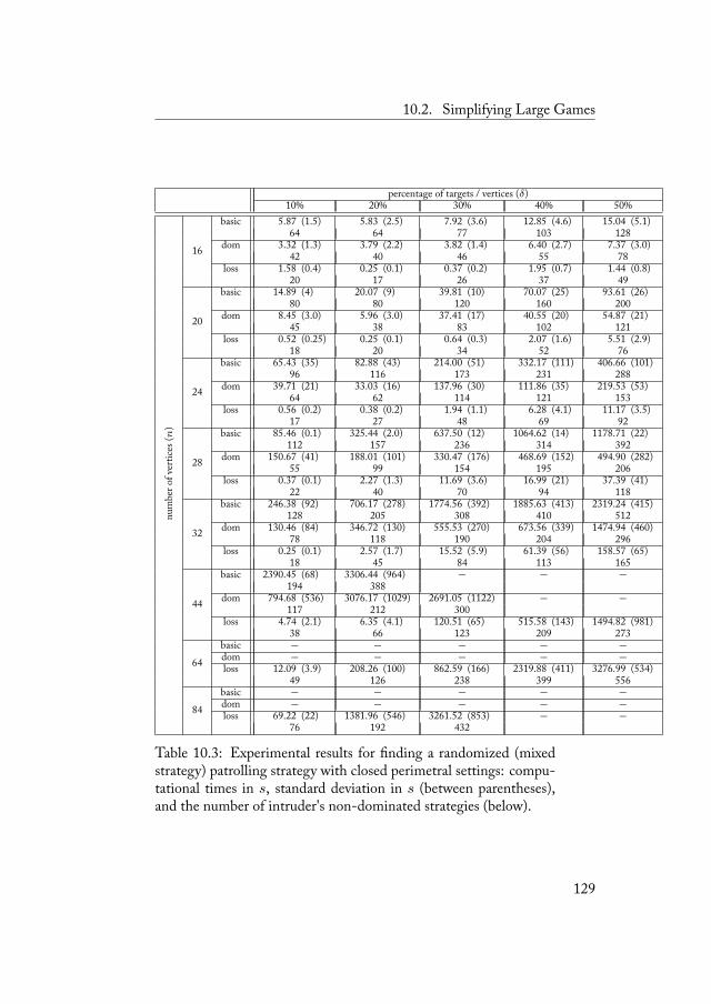
10.2. Simplifying Large Games

percentage of targets / vertices (δ)10% 20% 30% 40% 50%

num

bero

fver

tices

(n)

16

basic 5.87 (1.5) 5.83 (2.5) 7.92 (3.6) 12.85 (4.6) 15.04 (5.1)64 64 77 103 128

dom 3.32 (1.3) 3.79 (2.2) 3.82 (1.4) 6.40 (2.7) 7.37 (3.0)42 40 46 55 78

loss 1.58 (0.4) 0.25 (0.1) 0.37 (0.2) 1.95 (0.7) 1.44 (0.8)20 17 26 37 49

20

basic 14.89 (4) 20.07 (9) 39.81 (10) 70.07 (25) 93.61 (26)80 80 120 160 200

dom 8.45 (3.0) 5.96 (3.0) 37.41 (17) 40.55 (20) 54.87 (21)45 38 83 102 121

loss 0.52 (0.25) 0.25 (0.1) 0.64 (0.3) 2.07 (1.6) 5.51 (2.9)18 20 34 52 76

24

basic 65.43 (35) 82.88 (43) 214.00 (51) 332.17 (111) 406.66 (101)96 116 173 231 288

dom 39.71 (21) 33.03 (16) 137.96 (30) 111.86 (35) 219.53 (53)64 62 114 121 153

loss 0.56 (0.2) 0.38 (0.2) 1.94 (1.1) 6.28 (4.1) 11.17 (3.5)17 27 48 69 92

28

basic 85.46 (0.1) 325.44 (2.0) 637.50 (12) 1064.62 (14) 1178.71 (22)112 157 236 314 392

dom 150.67 (41) 188.01 (101) 330.47 (176) 468.69 (152) 494.90 (282)55 99 154 195 206

loss 0.37 (0.1) 2.27 (1.3) 11.69 (3.6) 16.99 (21) 37.39 (41)22 40 70 94 118

32

basic 246.38 (92) 706.17 (278) 1774.56 (392) 1885.63 (413) 2319.24 (415)128 205 308 410 512

dom 130.46 (84) 346.72 (130) 555.53 (270) 673.56 (339) 1474.94 (460)78 118 190 204 296

loss 0.25 (0.1) 2.57 (1.7) 15.52 (5.9) 61.39 (56) 158.57 (65)18 45 84 113 165

44

basic 2390.45 (68) 3306.44 (964) − − −194 388

dom 794.68 (536) 3076.17 (1029) 2691.05 (1122) − −117 212 300

loss 4.74 (2.1) 6.35 (4.1) 120.51 (65) 515.58 (143) 1494.82 (981)38 66 123 209 273

64basic − − − − −dom − − − − −loss 12.09 (3.9) 208.26 (100) 862.59 (166) 2319.88 (411) 3276.99 (534)

49 126 238 399 556

84basic − − − − −dom − − − − −loss 69.22 (22) 1381.96 (546) 3261.52 (853) − −

76 192 432

Table 10.3: Experimental results for finding a randomized (mixedstrategy) patrolling strategy with closed perimetral settings: compu-tational times in s, standard deviation in s (between parentheses),and the number of intruder's non-dominated strategies (below).

129

. E E

is 93% and the min is < 1%). For all the settings solvable with dom,we compared the patroller's expected utility given by the strategiesreturned by dom with that given by the strategies returned by loss.We observed that the loss strategies are never worse more than 5%than the dom strategies (the average worsening is 2.5%). ereforewe can say that, for closed perimetral settings, loss configuration pro-vides a very good approximation of the best patrolling strategy in areasonably short time.

130

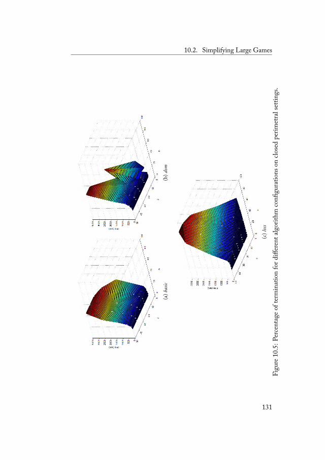
10.2. Simplifying Large Games

(a)b

asic

(b)d

om

(c)loss

Figu

re10

.5:P

erce

ntag

eoft

erm

inat

ion

ford

iffer

enta

lgor

ithm

confi

gura

tions

onclo

sed

perim

etra

lset

tings

.

131

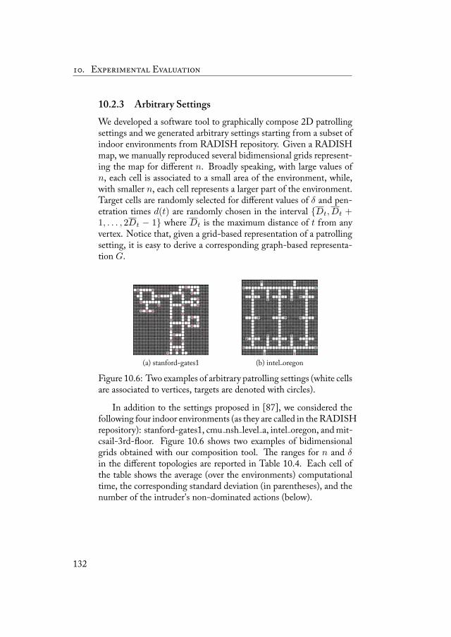
. E E

10.2.3 Arbitrary SettingsWe developed a software tool to graphically compose 2D patrollingsettings and we generated arbitrary settings starting from a subset ofindoor environments from RADISH repository. Given a RADISHmap, we manually reproduced several bidimensional grids represent-ing the map for different n. Broadly speaking, with large values ofn, each cell is associated to a small area of the environment, while,with smaller n, each cell represents a larger part of the environment.Target cells are randomly selected for different values of δ and pen-etration times d(t) are randomly chosen in the interval {Dt, Dt +1, . . . , 2Dt − 1} where Dt is the maximum distance of t from anyvertex. Notice that, given a grid-based representation of a patrollingsetting, it is easy to derive a corresponding graph-based representa-tion G.

(a) stanford-gates1 (b) intel oregon

Figure 10.6: Two examples of arbitrary patrolling settings (white cellsare associated to vertices, targets are denoted with circles).

In addition to the settings proposed in [87], we considered thefollowing four indoor environments (as they are called in theRADISHrepository): stanford-gates1, cmu nsh level a, intel oregon, andmit-csail-3rd-floor. Figure 10.6 shows two examples of bidimensionalgrids obtained with our composition tool. e ranges for n and δin the different topologies are reported in Table 10.4. Each cell ofthe table shows the average (over the environments) computationaltime, the corresponding standard deviation (in parentheses), and thenumber of the intruder's non-dominated actions (below).

132

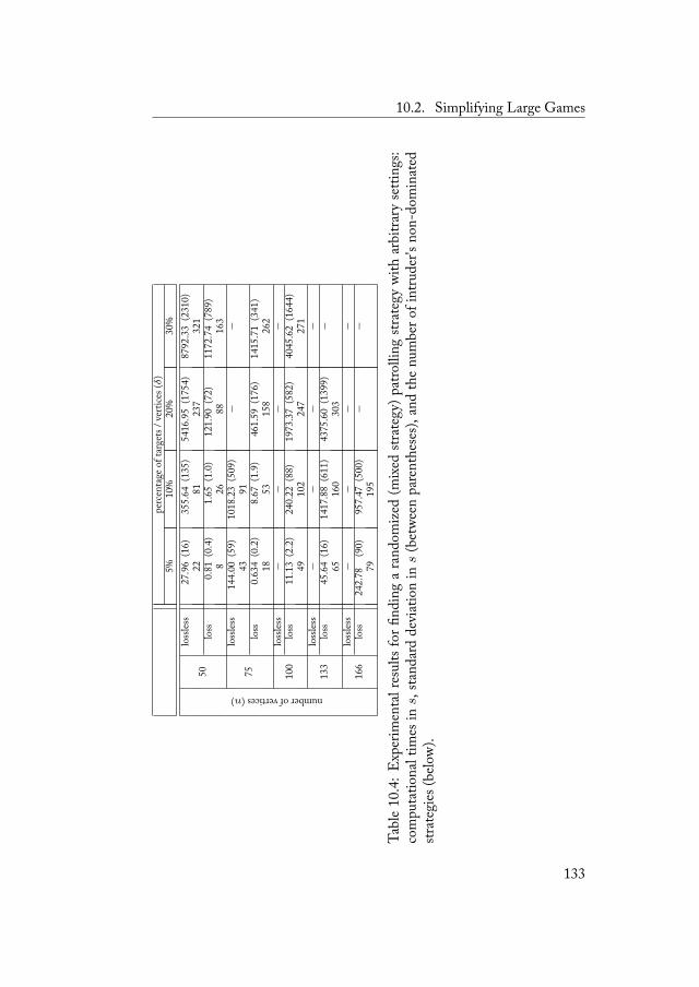
10.2. Simplifying Large Games

perc

enta

geof

targ

ets/

verti

ces(δ)

5%10

%20

%30

%

numberofvertices(n)

50lo

ssles

s27

.96

(16)

355.

64(1

35)

5416

.95

(175

4)87

92.3

3(2

310)

2281

237

321

loss

0.81

(0.4

)1.

65(1

.0)

121.

90(7

2)11

72.7

4(7

89)

826

8816

3

75lo

ssles

s14

4.00

(59)

1018

.23

(509

)−

−43

91lo

ss0.

634

(0.2

)8.

67(1

.9)

461.

59(1

76)

1415

.71

(341

)18

5315

826

2

100

lossles

s−

−−

−lo

ss11

.13

(2.2

)24

0.22

(88)

1973

.37

(582

)40

45.6

2(1

644)

4910

224

727

1

133

lossles

s−

−−

−lo

ss45

.64

(16)

1417

.88

(611

)43

75.6

0(1

399)

−65

160

303

166

lossles

s−

−−

−lo

ss24

2.78

(90)

957.

47(5

00)

−−

7919

5

Tabl

e10

.4:Exp

erim

enta

lres

ults

forfi

ndin

gara

ndom

ized

(mixed

strat

egy)

patro

lling

strat

egy

with

arbi

trary

setti

ngs:

com

puta

tiona

ltim

esin

s,sta

ndar

dde

viat

ion

ins

(bet

ween

pare

nthe

ses),

and

thenu

mbe

rofi

ntru

der's

non-

dom

inat

edstr

ateg

ies(

belo

w).

133

. E E

In this case we did not consider any time threshold in exper-iments, therefore memory was the only limited computational re-source. We solved the game instances only with the lossless and lossconfigurations (results with dom are worse than those with lossless,while with basic all the instances required more than 4 GB RAM).As it can be seen from Table 10.4, arbitrary settings turned out toless hard than the closed perimetral ones. By employing the losslessconfiguration we encountered a limit with n = 75 vertices (cells)with δ = 10% of targets. e loss configuration allowed us to solveinstances up to 166 cells with 10% of targets (also in this case thepatroller's expected utility worsening with respect to the lossless con-figuration is at most 5%). However, differently from the results ob-tained for open and closed perimetral settings, these computationallimits are less representative. e reason is that the particular topol-ogy of a setting has a very strong influence over the performance ofour algorithm. When dealing with arbitrary topologies, this preventsus from an exhaustive experimental analysis.

As a last experiment, we relaxed the penetration times in theabove instances such that they admit a pure strategy equilibriumwherethe intruder acts stay-out. We solved these instances with the losslessand loss configurations. e average computational times are close tothose reported in Table 10.4. ey are about 103 larger than thoseobtained with the algorithm we described in Chapter 8. In addi-tion, the solutions returned by the non-deterministic algorithm (be-ing Markovian) does not assure the patroller to capture the intruderwith a probability of one. is result justifies (a posteriori) our ap-proach to consider the problem of finding a deterministic patrollingstrategy as separate from the problem of finding a non-deterministicpatrolling strategy.

10.3 Toward a Real Deployment

In this last part of experiments we aim at shedding some light onthe real applicability of the patrolling strategies returned by the pro-posed game theoretical approach. A number of issues must be ad-dressed when moving from the theoretical model to a real imple-mentation. To the best of our knowledge, the only work that studiedgame-theoretical patrolling strategies in situations that are ''outside''the models assumptions is [3], where authors show how considering

134

10.3. Toward a Real Deployment

intruders with different degrees of knowledge about the patrollingstrategy can impact on the strategy's optimality. Following a similarapproach, we try to challenge some idealistic assumptions, includingthe following ones.

• e intruder is supposed to be a best responder, namely a ra-tional agent that maximizes its utility, given the strategy of thepatroller. is amounts to suppose that the patroller is facingthe strongest intruder that can play the game. However, in realsettings, the patroller can also face weaker intruders.

• e movements and the localization of the patrolling robot aresupposed to be error-free. is is obviously not true in a realsetting.

• e penetration times d(t) are known perfectly by both theplayers. In real settings, the values d(t) can be estimated, forexample, analyzing the integrity of windows and doors in nodest. Hence, values d(t) may be not precisely known by the play-ers.

• e intruder knows exactly the patroller's strategy. is as-sumption is realistic if we suppose, for example, that the in-truder can compute the optimal patrolling strategy in the sameway the patroller does or that it can look at the robot's controlsoftware. However, if we assume that the intruder derives suchknowledge only by observation, then its knowledge of the pa-trolling strategy will be approximated (at best), otherwise aninfinite observation time would be required. Note that know-ing the patrolling strategy {αi,j} does not mean to know thenext action of the patroller, but only the probability distribu-tion with which this action will be selected.

Other issues must be considered in a real implementation (sensors todetect intruders, battery, . . . ), but we deem that those listed above,and analyzed in the following, are among the most important onesand represent significant elements to assess the practical applicabilityof ourmodel. e results presented in the following involve strategiesobtained with the basic algorithm described in Section 7.3.

135

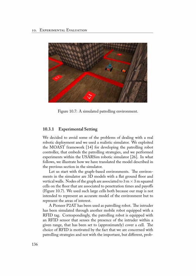
. E E

Figure 10.7: A simulated patrolling environment.

10.3.1 Experimental Setting

We decided to avoid some of the problems of dealing with a realrobotic deployment and we used a realistic simulator. We exploitedthe MOAST framework [14] for developing the patrolling robotcontroller, that embeds the patrolling strategies, and we performedexperiments within the USARSim robotic simulator [26]. In whatfollows, we illustrate how we have translated the model described inthe previous section in the simulator.

Let us start with the graph-based environments. e environ-ments in the simulator are 3D models with a flat ground floor andvertical walls. Nodes of the graph are associated to 3m× 3m squaredcells on the floor that are associated to penetration times and payoffs(Figure 10.7). We used such large cells both because our map is notintended to represent an accurate model of the environment but torepresent the areas of interest.

A Pioneer P2AT has been used as patrolling robot. e intruderhas been simulated through another mobile robot equipped with aRFID tag. Correspondingly, the patrolling robot is equipped withan RFID sensor that senses the presence of the intruder within agiven range, that has been set to (approximately) cover a cell. echoice of RFID is motivated by the fact that we are concerned withpatrolling strategies and not with the important, but different, prob-

136

10.3. Toward a Real Deployment

lems of detecting intruders. Note that the same technique is em-ployed in RoboCup Rescue Virtual Robots Competition to detectthe presence of victims.

e intruder's controller has been developed as a separate appli-cation that constantly ''observes'' the simulation and, according to thestrategy of the simulated intruder, decides when to attempt an intru-sion and in what cell. When an intrusion is attempted, the intruderrobot is inserted in the designated cell t. According to the theoreti-cal model, the simulated intruder ''appears'' at t. Starting from thatturn, if the penetration time d(t) expires before the patrolling robotcan sense the intruder's presence, then the intrusion is consideredsuccessfully completed and the outcome of the game is penetration-t.Otherwise, the intruder is detected and the outcome of the game isintruder-capture.

To quantify the advantages of the optimal patrolling strategy de-rived from our model over simpler patrolling strategies, we testedfour different patrollers. e optimal patroller moves according to theoptimal strategy {αij} returned by our model. At each turn, the nextcell to reach is randomly chosen according the probability distribu-tion defined by the {αij} values. en, the patroller moves from thecenter of its current cell to the center of the destination cell. e uni-form patroller determines the next cell to patrol extracting it from anuniform probability distribution over the cells adjacent to the currentone. Formally, if we call Ri the set of cells that are adjacent to celli, the strategy of the uniform patroller is defined as αij = 1/|Ri| ifj ∈ Ri and αij = 0 otherwise. e random patroller selects the nextcell according to a random probability distribution. Formally {αij}are randomly chosen with the constraint that

∑j∈Ri

αij = 1 andαij = 0 for every j /∈ Ri. Finally, the deterministic patroller cycli-cally follows the shortest path that visits all the cells. e differentpatrollers can be distinguished with respect to the amount of knowl-edge about the patrolling setting they use to compute their strategy.e optimal patroller has full knowledge of the environment topol-ogy and of the payoffs and penetration times. Differently, the otherpatrollers have only knowledge about the environment topology (forexample, penetration times are not considered by patrollers differentfrom the optimal one).

ree different intruders, with different intrusion strategies, havebeen defined. e optimal intruder is that assumed in our model. Itis the strongest intruder since it perfectly knows the strategy of the

137

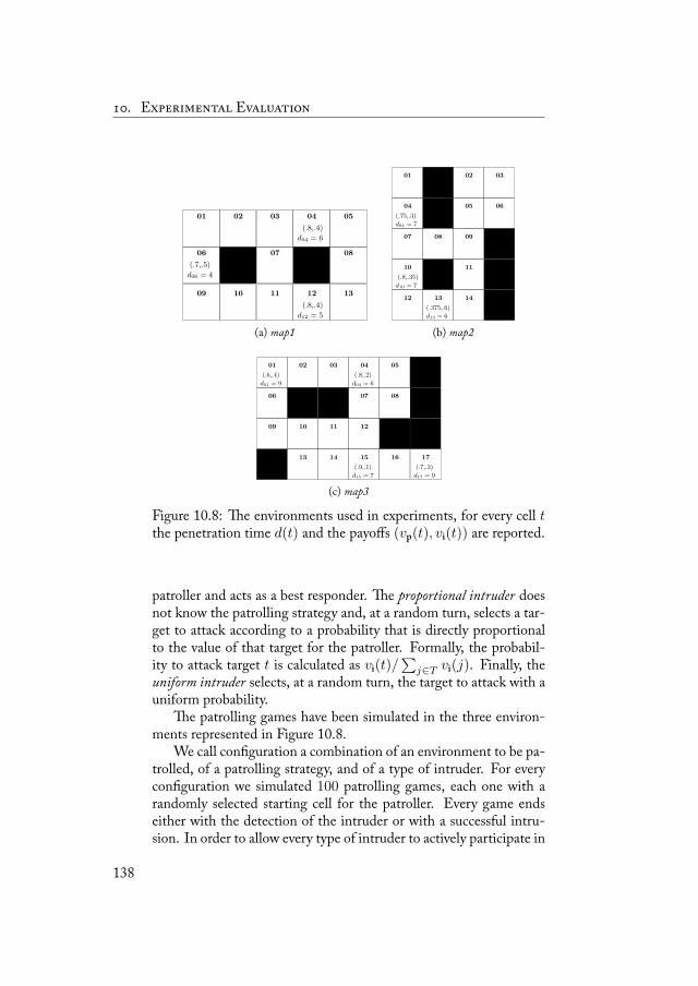
. E E

(.8,.4)

(.7,.5)

(.8,.4)

d12 = 5

d06 = 4

d04 = 6

01 02 03 04 05

06 07 08

09 10 11 12 13

(a) map1

(.8,.35)

(.75,.3)

(.375,.6)

d10 = 7

d04 = 7

d13 = 6

12

10

07

04

01

13

08

14

11

09

05

02

06

03

(b) map2

(.6,.4)

(.9,.1)

(.8,.2)

(.7,.3)

d01 = 9

d15 = 7

d04 = 6

d17 = 9

09

06

01

13

10

02

14

11

03

15

12

07

04

16

08

05

17

(c) map3

Figure 10.8: e environments used in experiments, for every cell tthe penetration time d(t) and the payoffs (vp(t), vi(t)) are reported.

patroller and acts as a best responder. e proportional intruder doesnot know the patrolling strategy and, at a random turn, selects a tar-get to attack according to a probability that is directly proportionalto the value of that target for the patroller. Formally, the probabil-ity to attack target t is calculated as vi(t)/

∑j∈T vi(j). Finally, the

uniform intruder selects, at a random turn, the target to attack with auniform probability.

e patrolling games have been simulated in the three environ-ments represented in Figure 10.8.

We call configuration a combination of an environment to be pa-trolled, of a patrolling strategy, and of a type of intruder. For everyconfiguration we simulated 100 patrolling games, each one with arandomly selected starting cell for the patroller. Every game endseither with the detection of the intruder or with a successful intru-sion. In order to allow every type of intruder to actively participate in

138

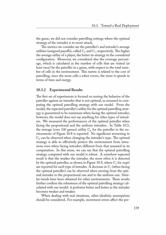
10.3. Toward a Real Deployment

the game, we did not consider patrolling settings where the optimalstrategy of the intruder is to never attack.

e metrics we consider are the patroller's and intruder's averageutilities (assigned payoffs), called Up and Ui, respectively. e higherthe average utility of a player, the better its strategy in the consideredconfiguration. Moreover, we considered also the coverage percent-age, which is calculated as the number of cells that are visited (atleast once) by the patroller in a game, with respect to the total num-ber of cells in the environment. is metric is related to the cost ofpatrolling, since the more cells a robot covers, the more it spends interms of time and energy.

10.3.2 Experimental Resultse first set of experiments is focused on testing the behavior of thepatroller against an intruder that is not optimal, as assumed in com-puting the optimal patrolling strategy with our model. From themodel, the expected patroller's utility for the optimal patrolling strat-egy is guaranteed to be maximum when facing the optimal intruder;however, the model does not say anything for other types of intrud-ers. We measured the performances of the optimal patroller whenfacing the proportional and the uniform intruders. In Table 10.5,the average (over 100 games) utility Up for the patroller in the en-vironments of Figure 10.8 is reported. No significant worsening inUp can be observed when changing the intruder's type. e optimalstrategy is able to effectively protect the environment from intru-sions even when facing intruders different from that assumed in itscomputation. In this sense, we can say that the optimal patrollingstrategy computed with our model is robust. A somehow expectedresult is that the weaker the intruder, the more often it is detectedby the optimal patroller, as shown in Figure 10.9, where Ui for map1are reported for each type of intruder. A decrease in Ui (when facingthe optimal patroller) can be observed when moving from the opti-mal intruder to the proportional one and to the uniform one. Simi-lar trends have been obtained for other environments. ese resultsfurther confirm the robustness of the optimal patrolling strategy cal-culated with our model: it performs better and better as the intruderbecomes weaker and weaker.

When dealing with real situations, other idealistic assumptionsshould be considered. For example, movement errors affect the per-

139

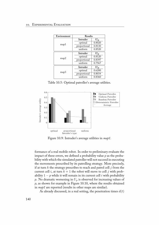
. E E

Environment Results

map1

Intruder Up

optimal 0.8020proportional 0.8130

uniform 0.8520

map2

Intruder Up

optimal 0.8120proportional 0.8397

uniform 0.7567

map3

Intruder Up

optimal 0.6200proportional 0.8034

uniform 0.8360

Table 10.5: Optimal patroller's average utilities.

optimal proportional uniform

0

0.1

0.2

0.3

0.4

0.5

0.6

Intruder’s type

Intruder’saverageutility

Optimal PatrollerUniform Patroller

Random PatrollerDeterministic Patroller

Average

Figure 10.9: Intruder's average utilities in map1.

formance of a real mobile robot. In order to preliminary evaluate theimpact of these errors, we defined a probability value p as the proba-bility with which the simulated patroller will not succeed in executingthe movements prescribed by its patrolling strategy. More precisely,if at turn k the strategy prescribes to reach and patrol cell j from thecurrent cell i, at turn k + 1 the robot will move to cell j with prob-ability 1− p while it will remain in its current cell i with probabilityp. No dramatic worsening in Up is observed for increasing values ofp, as shown for example in Figure 10.10, where the results obtainedin map1 are reported (results in other maps are similar).

As already discussed, in a real setting, the penetration times d(t)

140

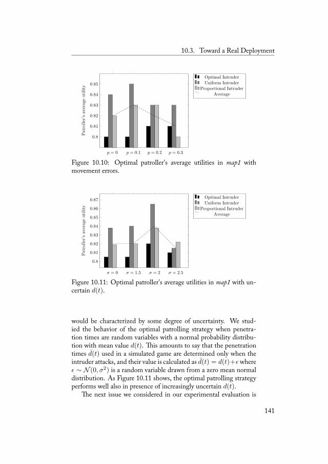
10.3. Toward a Real Deployment

p = 0 p = 0.1 p = 0.2 p = 0.3

0.8

0.81

0.82

0.83

0.84

0.85Patroller’saverageutility

Optimal Intruder

Uniform IntruderProportional Intruder

Average

Figure 10.10: Optimal patroller's average utilities in map1 withmovement errors.

σ = 0 σ = 1.5 σ = 2 σ = 2.5

0.8

0.81

0.82

0.83

0.84

0.85

0.86

0.87

Patroller’saverageutility

Optimal Intruder

Uniform IntruderProportional Intruder

Average

Figure 10.11: Optimal patroller's average utilities in map1 with un-certain d(t).

would be characterized by some degree of uncertainty. We stud-ied the behavior of the optimal patrolling strategy when penetra-tion times are random variables with a normal probability distribu-tion with mean value d(t). is amounts to say that the penetrationtimes d(t) used in a simulated game are determined only when theintruder attacks, and their value is calculated as d(t) = d(t)+εwhereε ∼ N (0, σ2) is a random variable drawn from a zero mean normaldistribution. As Figure 10.11 shows, the optimal patrolling strategyperforms well also in presence of increasingly uncertain d(t).

e next issue we considered in our experimental evaluation is

141

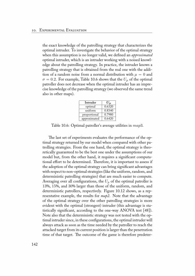
. E E

the exact knowledge of the patrolling strategy that characterizes theoptimal intruder. To investigate the behavior of the optimal strategywhen this assumption is no longer valid, we defined an approximatedoptimal intruder, which is an intruder working with a noised knowl-edge about the patrolling strategy. In practice, the intruder knows apatrolling strategy that is obtained from the real one with the addi-tion of a random noise from a normal distribution with µ = 0 andσ = 0.2. For example, Table 10.6 shows that the Up of the optimalpatroller does not decrease when the optimal intruder has an impre-cise knowledge of the patrolling strategy (we observed the same trendalso in other maps).

Intruder Up

optimal 0.6320uniform 0.8340

proportional 0.7980approximated 0.6420

Table 10.6: Optimal patroller's average utilities in map3.

e last set of experiments evaluates the performance of the op-timal strategy returned by our model when compared with other pa-trolling strategies. From the one hand, the optimal strategy is theo-retically guaranteed to be the best one under the assumptions of ourmodel but, from the other hand, it requires a significant computa-tional effort to be determined. erefore, it is important to assess ifthe adoption of the optimal strategy can bring significant advantageswith respect to non-optimal strategies (like the uniform, random, anddeterministic patrolling strategies) that are much easier to compute.Averaging over all configurations, the Up of the optimal patroller is13%, 15%, and 30% larger than those of the uniform, random, anddeterministic patrollers, respectively. Figure 10.12 shows, as a rep-resentative example, the results for map2. Note that the advantageof the optimal strategy over the other patrolling strategies is moreevident with the optimal (strongest) intruder (this advantage is sta-tistically significant, according to the one-way ANOVA test [48]).Note also that the deterministic strategy was not tested with the op-timal intruder since, in these configurations, the optimal intruder willalways attack as soon as the time needed by the patroller to reach theattacked target from its current position is larger than the penetrationtime of that target. e outcome of the game is therefore predeter-

142

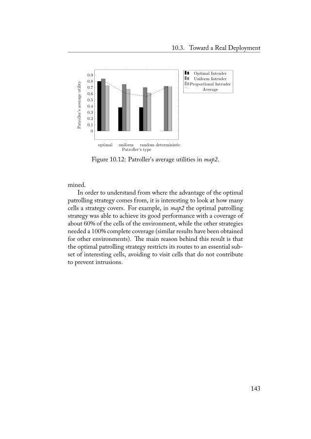
10.3. Toward a Real Deployment

optimal uniform random deterministic

0

0.1

0.2

0.3

0.4

0.5

0.6

0.7

0.8

0.9

Patroller’s type

Patroller’saverageutility

Optimal Intruder

Uniform IntruderProportional Intruder

Average

Figure 10.12: Patroller's average utilities in map2.

mined.In order to understand from where the advantage of the optimal

patrolling strategy comes from, it is interesting to look at how manycells a strategy covers. For example, in map2 the optimal patrollingstrategy was able to achieve its good performance with a coverage ofabout 60% of the cells of the environment, while the other strategiesneeded a 100% complete coverage (similar results have been obtainedfor other environments). e main reason behind this result is thatthe optimal patrolling strategy restricts its routes to an essential sub-set of interesting cells, avoiding to visit cells that do not contributeto prevent intrusions.

143

Conclusions 11

Navigation strategies are a fundamental component in building au-tonomy for mobile robots. ey allow a robot to autonomously de-cide where to move in the environment with the purpose of accom-plishing some task. A challenging problem is the definition of goodnavigation strategies that aim at optimizing some performance met-ric related to the task. In this thesis, we suggested to cast this prob-lem in a general and application-independent framework representedby decision-theoretical techniques. e technical contributions pre-sented in this thesis have considered the definition of navigation strate-gies from this perspective and addressed two applicative domains,exploration and patrolling, that constitute representative scenarioswhere the availability of effective navigation strategies is a key fac-tor.

In exploration, a mobile robot is deployed in an initially unknownenvironment with the goal of autonomously detect the free space andthe obstacles. e exploration strategy is the method with which therobot selects the next observation location to reach in order to sensethe environment. We considered two particular scenarios where ex-ploration is aimed at two different purposes, namely building a mapand searching for the presence of human victims on a disaster site.Multi-Criteria Decision Making (MCDM) is proposed as a gen-eral and flexible decision-theoretical technique to evaluate and select

145

. C

observation locations. e main advantage of MCDM is the pos-sibility to combine multiple evaluation criteria into a global utilityfunction. is method differs from the mainstream approach, whereexploration strategies are based on ad hoc utility functions, in generalhardly applicable to situations different from those they have beentailored for. In our experimental analysis we showed that MCDMallow to define exploration strategies that have good performance,while providing a flexible way to define the trade-off between a set ofcriteria for evaluating candidate locations.

In robotic patrolling, a mobile robot moves within a known en-vironment with the objective of avoiding the entrance of intruders.e patrolling strategy drives the robot in deciding the environment'spositions to reach and monitor and, obviously, has a strong impactover the resulting protection level. To deal with the problem of defin-ing good patrolling strategies we adopt, following an approach thatrecently received much interest, a game-theoretical framework. eintruder is explicitly considered as a rational agent acting against thepatroller. It is assumed to have full knowledge of the the patroller'sstrategy. A game model is build, where the patroller and the intruderact one against each other. e optimal patrolling strategy can becomputed by searching for the equilibrium of this game. We pro-posed a general game model to capture more complex scenarios withrespect to those proposed in literature, considering arbitrary graph-like environments. In our experimental activities we show that theproposed techniques can enable the efficient computation of optimalpatrolling strategies in realistic settings. Moreover, we dealt with theproblem of employing this approach in realistic settings, where thecomputational effort needed to compute the optimal strategy and theinfringement of some idealized assumptions can represent a signifi-cant limitation.

With respect to the general objectives of this thesis, we drawthe following conclusions. e decision theoretical techniques stud-ied in this work turned out to be an effective tool for the definitionof navigation strategies in the two applicative contexts we consid-ered. e results obtained suggest that a global characterization ofthe problem under a decision theoretical perspective can introducesome advantages. e use of MCDM for exploration allowed us toeasily define, with a single method, exploration strategies adaptableto different purposes (map building and rescue). e flexibility of theproposed approach together with the comparable or, in some cases,

146

better performance we obtained with respect to the strategies pro-posed in literature make MCDM a profitable method for the def-inition of navigation strategies in exploration. Developing a gametheoretical framework for robotic patrolling, we showed how a com-plex robotic scenario, characterized by decision making in presenceof multiple interacting agents. can be properly modeled within adecision-theoretical framework. In this way, the availability of wellstudied game-theoretical techniques such as dominance and abstrac-tions allowed us to improve the efficiency in computing patrollingstrategies. is strongly contributed in achieving the goal of beingable to deal with realistic situations, characterized by relatively largeenvironments.

Several issues are worth further investigation both in autonomousexploration and in robotic patrolling. Le us start from autonomousexploration. To use MCDM with large set of criteria, we need to gobeyond the manual selection of weights. Different approaches canbe investigated for this goal, such as constraint satisfaction (as brieflydiscussed in Section 3.2) or machine learning techniques. More-over, a complete integration of MCDM within a multirobot scenarioneeds further work. In this case, task-assignment techniques can bestudied and tailored to the problem of assigning observation loca-tions to a group of robots that use MCDM to evaluate the utilityof a given robot-location assignment. Another interesting directionis related to decisions that can be revised, i.e., allowing the robot toeventually change a decision before having reached the selected ob-servation location by considering the new knowledge acquired fromthe last decision. is issue could allow the robot to limit the poten-tial performance worsening deriving from a previous ''wrong'' choice.For example, in the case of continuous perception, the robot couldselect a new observation location before having reached the previ-ously selected one as it discovers, moving along the path, that nonew information can be obtained by continuing on that way. Revis-ing decisions would introduce a computational cost and a trade-offwith potential benefits has to be addressed. Finally, other settingsin which exploration is employed can be interesting for assessing theproperties of MCDM, some example are planetary exploration, gasor fire source localization, or coverage.

Switching to robotic patrolling, abstractions constitute an inter-esting topic to investigate. Going beyond the best abstractions in

147

. C

terms of reduction of computational time (as we discussed in thiswork), it would be possible to studying abstractions that take intoaccount the patroller's expected utility, thus searching for the bestabstraction for a given trade-off between computational time andexpected utility. Another important issue is the development of adhoc techniques to improve the resolution process for finding equilib-rium patrolling strategies allowing to push forward the limit on themaximum size of computationally affordable game instances. Tech-niques could come from the operational research literature, includingcolumn generation or cut generation techniques. A key factor thatcould improve the ''on-the-field'' performance of our model is to en-rich it and capture more realistic situations. Some of these issueshave already been partially addressed. ey include refining the in-truder's movement model by allowing it to move along paths [20],limiting the observation capabilities of the intruder when starting anattack [20], considering the situationwherein there is a delay betweenthe turn at which the intruder decides to enter and the turn at whichit actually enters [19]. Finally, one of the most challenging exten-sions is represented by the multirobot case, where the patrolling taskhas to be performed by a team of cooperating robots. We preliminaryaddressed this issues in [21] by studying the problem of computingthe minimum number of robots to patrol a given environment andby investigating how different degrees of coordination between therobots can affect the process of computing a corresponding patrollingstrategy.

Considering navigation strategies from a decision-theoretical pointof view, we see three main future research directions. e first one in-volves the development of a general decision-theoretical frameworkaimed at characterizing the problem of defining a navigation strategyfor a given application under a set decision-theoretical features. Apossible approach to deal with this problem can be to start from whatwe presented in Section 1.3 where we list some significant dimen-sions according to which a navigation strategy can be classified. esecond direction is considering new kinds (according to dimensionsof Section 1.3) of problems within new applicative contexts in orderto further assess the applicability of a decision-theoretical approachfor navigation strategies. Finally, a last challenge involves experi-mental evaluation methodologies for navigation strategies. Defininggood experimental methodologies to evaluate and compare differentnavigation strategies still represents an important open problem.

148

Proofs A

A.1 Proof of Proposition 7.3.6

Consider the setting of Figure 7.1 with the following penetrationtimes:

d(06) = 14 d(08) = 18 d(12) = 23 d(14) = 22 d(18) = 18

is game admits a leader-follower deterministic patrolling strategywhere the patroller follows a cycle over the targets (i.e., 14, 08, 06, 18,12, 18, 06, 08, 14) moving along the shortest paths. e best in-truder's action is stay-out independently of the value of ε, otherwiseit would be captured with a probability of one. It can be easily ob-served that this patrolling strategy implies l = 2. Suppose to applyFormulation 7.3.3 to such a game. We can show that we can al-ways find a value of ε such that there is no patrolling strategy withl = 1 such that stay-out is the intruder's best response. Consideraction enter-when(06, 23), the associated capture probability is al-ways smaller than one when l = 1. Indeed, the values α11,i withi ∈ {06, 12, 18} are strictly positive to assure that the patroller cancover all the targets. en, by Markov chains, it follows that theprobability that the patroller reaches vertex 06 starting from vertex23 within 9 turns is strictly smaller than one. We can always find astrictly positive value of ε such that, when the patroller follows the

149

A. P

strategy with l = 1, the intruder strictly prefers to attack a targetrather than not to attack. Since the intruder will attack and theprobability of being captured is strictly smaller than one, the util-ity expected by the patroller from following the strategy with l = 1will be strictly smaller than the expected utility from following thedeterministic equilibrium strategy with l = 2. �

A.2 Proof ofeorem 8.1.4

We prove the NP-completeness by reducing the Directed Hamilto-nian Circuit problem (DHC) [75] to the DET-STRAT problem.DHC is the problem of determining if an Hamiltonian path, i.e.,a path that visits each vertex exactly once, exists in a given directedgraph. is is a well-known NP-complete problem. Let us considera generic instance of the DHC problem given by a directed graphGh = (Vh, Ah) where Vh is the set of vertices and Ah is the setof arcs. In order to prove that DHC can be reduced to the DET-STRAT problem, we show that for every instance Gh of the DHCproblem an instance G′s of the DET-STRAT problem can be builtin polynomial time and that by solving the DET-STRAT problemon G′s we obtain also a solution for the DHC problem on Gh. Aninstance G′s = (Ts, As, ws, ds) can be easily constructed from Gh inthe following way: Ts = Vh, As = Ah, for every v ∈ Ts we imposed(v) = |Vh| and ws(v, v

′) = 1 for all v, v′ ∈ Ts. It is straight-forward to see that a solution of G′s, if it exists, is an Hamiltoniancycle. Indeed, since the relative deadline of every target is equal tothe number of targets, a deterministic equilibrium strategy shouldvisit each target exactly once, otherwise at least one relative deadlinewould be violated (being ws(v, v

′) = 1 for all v, v′ ∈ Ts). erefore,computing the solution for G′s provides by construction a solutionfor Gh or, in other words, the DHC problem can be reduced to theDET-STRAT problem, proving its NP-completeness (the proof iscompleted by noting that it is trivially polynomial to verify that agiven sequence of vertices is a solution of the DET-STRAT prob-lem). �

150

A.3. Proof of eorem 8.1.5

A.3 Proof ofeorem 8.1.5

In order to prove the theorem it is sufficient to prove that, if a prob-lem is solvable, then there exists a solution σ in which there is at leasta vertex that only appears once, excluding σ(s). Indeed, if this state-ment holds then the maximum temporal length of σ is bounded byd(i) where i is the vertex that appears only one time in σ. It easilyfollows that, in the worst case, the maximum temporal length of σ ismaxt∈T {d(t)}.

We now prove that, if the problem is solvable, then there is a so-lution in which at least a vertex appears only once. To prove this,we consider a solution σ wherein σ(1) is the vertex with the mini-mum relative deadline, i.e, σ(1) = argmint∈T {d(t)}. (Notice thatthis assignment does not preclude finding a solution.) We call k theminimum integer such that all the vertices appear in the subsequenceσ(1)− σ(k). We show that, if the problem is solvable, then it is notnecessary that vertex v = σ(k) appears again after k. A visit to vafter k would be observed if either it is necessary to pass through v toreach σ(1) or it is necessary to re-visit v, due to its relative deadline,before σ(1). However, since all the vertices but v = σ(k) are vis-ited before k, all the vertices but v can be visited without necessarilyvisiting v. Furthermore, the deadline of σ(1) is by hypothesis harderthan σ(k)'s one and then the occurrence of v = σ(k) after k is notnecessary. erefore, vertex σ(k) occurs only one time. �

A.4 Proof ofeorem 8.2.1

We initially prove the soundness of the algorithm. We need to provethat all the solutions it produces satisfy constraints (8.1)-(8.5). Con-straints (8.1), (8.2), and (8.5) are satisfied by Algorithm 3. If at leastone of them does not hold, no solution is produced. e satisfactionof constraints (8.3) is assured by Algorithm 4 in Step 3, while thesatisfaction of constraints (8.4) is assured by Algorithm 4 in Steps 6and 9.

In order to prove completeness we need to show that the algo-rithm produces a solution whenever at least one exists. In the al-gorithm there are only two points in which a candidate solution isdiscarded. e first one is the forward checking in Algorithm 4.Indeed, it iteratively applies constraints (8.4)-(8.5) to a partial se-

151

A. P

quence σ exploiting a heuristic over the future weights (i.e., the timespent to visit the successive vertices). Since the employed heuristicis admissible, no feasible candidate solution can be discarded. esecond point is the stopping criterion in Algorithm 3: when all thevertices occur in σ (at least once) and the first and the last vertexin σ are equal, no further successor is considered and the search isstopped. If σ satisfies all the constraints, then σ is a solution, oth-erwise backtracking is performed. We show that, if a solution canbe found without stopping the search at this point, then a solutioncan be found also by stopping the search and backtracking (the viceversa does not hold). is issue is of paramount importance since itassures that the algorithm terminates (in Section 8.2.1 we provide anexample in which, without this stopping criterion, the search couldnot terminate). Consider a σ such that σ(1) = σ(s) and includingall the vertices in T . e search subtree following σ(s) and producedby the proposed algorithm is (non-strictly) contained in the searchtree following from σ(1). is is because the constraints consideredby the forward checking from σ(s) on are (non-strictly) harder thanthose considered from σ(1) to σ(s). e increased hardness is due tothe activation of constraints (8.4) that are needed given that at leastone occurrence of each vertex is in σ. us, if a solution can be foundby searching from σ(s), then a shorter solution can be found by stop-ping the search at σ(s) and backtracking. is concludes the proofof completeness. �

A.5 Proof ofeorem 9.1.1

Call z a vertex that is not on any shortest path between any pair oftargets. If a strategy σp prescribes that the patroller can make ac-tion move(z) with a strictly positive probability, then it can be easilyobserved that, if the patroller does not make such action, it cannotdecrease its expected utility. Indeed, the intruder capture probabilityPc(t, x) for any t ∈ T and x ∈ V cannot decrease since visiting zwould introduce an unnecessary temporal cost. �

A.6 Proof ofeorem 9.1.2

e proof is trivial. When the patroller moves along Q, the intrudercapture probabilities are not smaller than in the case in which the

152

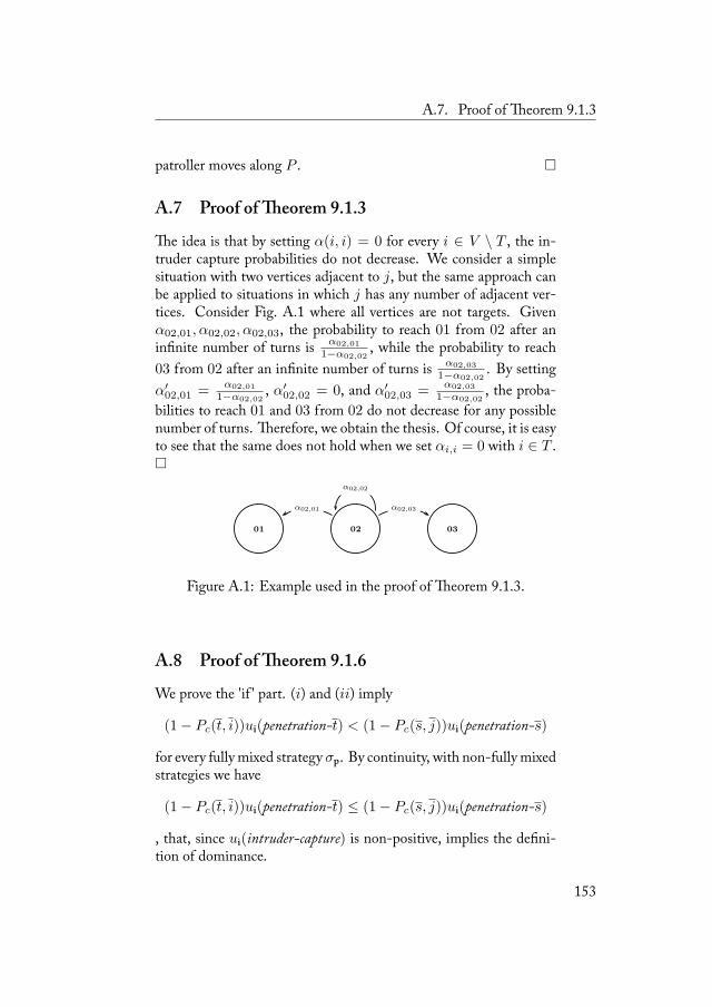
A.7. Proof of eorem 9.1.3

patroller moves along P . �

A.7 Proof ofeorem 9.1.3

e idea is that by setting α(i, i) = 0 for every i ∈ V \ T , the in-truder capture probabilities do not decrease. We consider a simplesituation with two vertices adjacent to j, but the same approach canbe applied to situations in which j has any number of adjacent ver-tices. Consider Fig. A.1 where all vertices are not targets. Givenα02,01, α02,02, α02,03, the probability to reach 01 from 02 after aninfinite number of turns is α02,01

1−α02,02, while the probability to reach

03 from 02 after an infinite number of turns is α02,03

1−α02,02. By setting

α′02,01 =α02,01

1−α02,02, α′02,02 = 0, and α′02,03 =

α02,03

1−α02,02, the proba-

bilities to reach 01 and 03 from 02 do not decrease for any possiblenumber of turns. erefore, we obtain the thesis. Of course, it is easyto see that the same does not hold when we set αi,i = 0 with i ∈ T .�

01 02 03

α02,01

α02,02

α02,03

Figure A.1: Example used in the proof of eorem 9.1.3.

A.8 Proof ofeorem 9.1.6

We prove the 'if ' part. (i) and (ii) imply

(1− Pc(t, i))ui(penetration-t) < (1− Pc(s, j))ui(penetration-s)

for every fully mixed strategy σp. By continuity, with non-fully mixedstrategies we have

(1− Pc(t, i))ui(penetration-t) ≤ (1− Pc(s, j))ui(penetration-s)

, that, since ui(intruder-capture) is non-positive, implies the defini-tion of dominance.

153

A. P

We prove the 'only if ' part of (i). For all the possible patrollingsettings, if ui(penetration-t) > ui(penetration-s), it is possible tofind a fully mixed strategy σp such that EUi(enter-when(t, i)) >

EUi(enter-when(s, j)) in the following way. We set all the prob-abilities leading to s from j equal to 1 − ε with ε > 0 arbitrar-ily small. If the path connecting t to i is not strictly contained inthe path connecting s to j, then we can set some probability in thepath connecting t to i equal to ε and thus (1 − Pc(t, i)) ' 1 and(1 − Pc(s, j)) ' 0, satisfying the previous inequality. If the pathconnecting t to i is strictly contained in the path connecting s to j,we have (1 − Pc(t, i)) < (1 − Pc(s, j)). However, we can set theprobabilities leading to s from t equal to 1− ε′ such that Pc(s, j) ≥(1− ε′)kPc(t, i) where k is the distance between t and s. It is alwayspossible to find a ε′ such thatPc(s, j)−Pc(t, i) is arbitrarily small andsince the difference between ui(penetration-t) and ui(penetration-s)is finite, EUi(enter-when(t, i)) > EUi(enter-when(s, j)).

We prove the 'only if ' part of (ii). If there exists a strategy σpsuch that Pc(t, i) < Pc(s, j), then the path connecting t to i is notstrictly contained in the path connecting s to j. In this case, wecan find a σp (as we discussed above) such that (1 − Pc(t, i)) ' 1

and (1 − Pc(s, j)) ' 0 and therefore action enter-when(t, i) is notdominated. �

A.9 Proof ofeorem 9.1.10

e proof is trivial. e intruder's action enter-when(t, t) being dom-inated, the intruder will never enter t when the patroller is in t.erefore, setting αt,t = 0, the probability that the intruder willbe captured when it enters t will never decrease. �

A.10 Proof ofeorem 9.2.8

e proof has two steps. In the first one, we show that, after the ap-plication of the lossless abstractions, the set of intruder's dominatedstrategies is left unchanged, and therefore we can focus only on thedominant strategies. In the second one, we show that for any strategyσ in the non-abstracted game, we can find, by solving the abstractedgame, a strategy σ′ that gives the patroller a utility not smaller thanthat σ gives. With abuse of notation, we denote by Pc(x, y, z) the

154

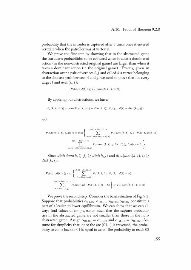
A.10. Proof of eorem 9.2.8

probability that the intruder is captured after z turns once it enteredvertex x when the patroller was at vertex y.

We prove the first step by showing that in the abstracted gamethe intruder's probabilities to be captured when it takes a dominatedaction (in the non-abstracted original game) are larger than when ittakes a dominant action (in the original game). Exactly, given anabstraction over a pair of vertices i, j and called k a vertex belongingto the shortest path between i and j, we need to prove that for everytarget t and dom(k, t):

Pc(k, t, d(t)) ≥ Pc(dom(k, t), t, d(t))

By applying our abstractions, we have:

Pc(k, t, d(t)) = max{Pc(i, t, d(t)− dist(k, i)), Pc(j, t, d(t)− dist(k, j))}

and

Pc(dom(k, t), t, d(t)) = max{

d(t)−dist(i,t)∑h=dist(dom(k,t),i)

Pr(dom(k, t), i, h)·Pc(i, t, d(t)−h),

d(t)−dist(j,t)∑h=dist(dom(k,t),j)

Pr(dom(k, t), j, h) · Pc(j, t, d(t)− h)

}

Since dist(dom(k, t), j) ≥ dist(k, j) and dist(dom(k, t), i) ≥dist(k, i):

Pc(k, t, d(t)) ≥ max{

d(t)−dist(i,t)∑h=dist(k,i)

Pr(k, i, h) · Pc(i, t, d(t)− h),

d(t)−dist(j,t)∑h=dist(k,j)

Pr(k, j, h) · Pc(j, t, d(t)− h)

}≥ Pc(dom(k, t), t, d(t))

Weprove the second step. Consider the basic situation of Fig. 9.3.Suppose that probabilities α01,02, α02,01, α02,03, α03,02 constitute apart of a leader-follower equilibrium. We can show that we can al-ways find values of α01,03, α03,01 such that the capture probabili-ties in the abstracted game are not smaller than those in the non-abstracted game. Assign α01,03 = α01,02 and α03,01 = α03,02. As-sume for simplicity that, once the arc (01, ·) is traversed, the proba-bility to come back to 01 is equal to zero. e probability to reach 03

155

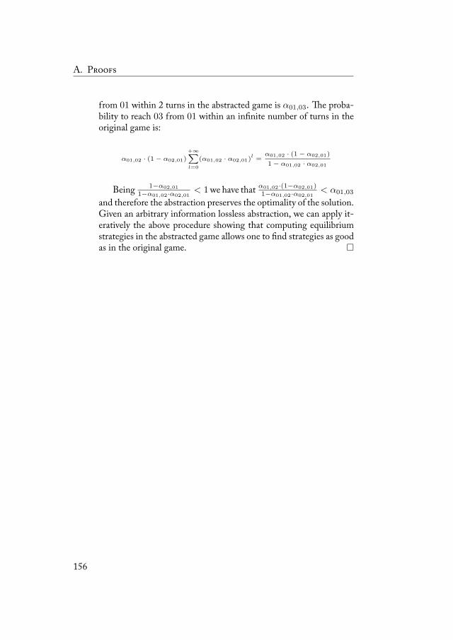
A. P

from 01 within 2 turns in the abstracted game is α01,03. e proba-bility to reach 03 from 01 within an infinite number of turns in theoriginal game is:

α01,02 · (1− α02,01)

+∞∑l=0

(α01,02 · α02,01)l=

α01,02 · (1− α02,01)

1− α01,02 · α02,01

Being 1−α02,01

1−α01,02·α02,01< 1we have that α01,02·(1−α02,01)

1−α01,02·α02,01< α01,03

and therefore the abstraction preserves the optimality of the solution.Given an arbitrary information lossless abstraction, we can apply it-eratively the above procedure showing that computing equilibriumstrategies in the abstracted game allows one to find strategies as goodas in the original game. �

156

Bibliography

[1] N. Agmon. On events in multi-robot patrol in adversarial en-vironments. In Proceedings of International Joint Conference onAutonomous Agents and Multi-Agent Systems (AAMAS), pages591--598, Toronto, Canada, 2010.

[2] N. Agmon, S. Kraus, andG. Kaminka. Multi-robot perimeterpatrol in adversarial settings. In Proceedings of the IEEE Inter-national Conference on Robotics and Automation (ICRA), pages2339--2345, Pasadena, USA, 2008.

[3] N. Agmon, V. Sadov, G. Kaminka, and S. Kraus. e impactof adversarial knowledge on adversarial planning in perimeterpatrol. In Proceedings of the International Joint Conference onAutonomous Agents and Multi Agent Systems (AAMAS), pages55--62, Estoril, Portugal, May 12-16 2008.

[4] N. Agmon, S. Kraus, and G. Kaminka. Uncertainties in ad-versarial patrol. In Proceedings of the International Joint Confer-ence on Autonomous Agents and Multi Agent Systems (AAMAS),pages 1267--1268, Budapest, Hungary, May 10-15 2009.

[5] N. Agmon, S. Kraus, G. Kaminka, and V. Sadov. Adversarialuncertainty in multi-robot patrol. In Proceedings of the Inter-national Joint Conference on Artificial Intelligence (IJCAI), pages1811--1817, 2009.

[6] A. Almeida, G. Ramalho, H. Santana, P. Tedesco,T. Menezes, V. Corruble, and Y. Chevaleyre. Recent ad-vances on multi-agent patrolling. In Proceedings of the Brazil-ian Symposium on Artificial Intelligence (SBIA), volume LNCS3171, pages 126--138, 2004.

157

B

[7] F. Amigoni. Experimental evaluation of some explorationstrategies for mobile robots. In Proceedings of IEEE Inter-national Conference on Robotics and Automation (ICRA), pages2818--2823, 2008.

[8] F. Amigoni and A. Gallo. A multi-objective exploration strat-egy for mobile robots. In Proceedings of IEEE InternationalConference on Robotics and Automation (ICRA), pages 3861--3866, 2005.

[9] F. Amigoni, V. Caglioti, and U. Galtarossa. A mobile robotmapping system with an information-based exploration strat-egy. In Proceedings of International Conference on Informaticsin Control, Automation and Robotics (ICINCO), pages 71--78,2004.

[10] F. Amigoni, N. Gatti, and A. Ippedico. A game-theoretic ap-proach to determining efficient patrolling strategies for mobilerobots. In Proceedings of the IEEE/WIC/ACM InternationalConference on Agent Intelligent Technology (IAT), pages 500--503, Sydney, Australia, December 9-12 2008.

[11] F. Amigoni, N. Basilico, and N. Gatti. Finding the op-timal strategies in robotic patrolling with adversaries intopologically-represented environments. In Proceedings ofthe IEEE International Conference on Robotics and Automation(ICRA), pages 819--824, Kobe, Japan, May 12-17 2009.

[12] F. Amigoni, N. Basilico, N. Gatti, A. Saporiti, and S. Troiani.Moving game theoretical patrolling strategies from theory topractice: An usarsim simulation. In Proceedings of IEEE Inter-national Conference on Robotics and Automation (ICRA), pages426 -- 431, 2010.

[13] B. Balaguer, S. Balakirsky, S. Carpin, and A. Visser. Evaluat-ingmaps produced by urban search and rescue robots: Lessonslearned from robocup. Autonomous Robots, 27(4):449--464,2009.

[14] S. Balakirsky, C. Scrapper, and E. Messina. Mobility openarchitecture simulation and tools environment. In Proceedingsof the International Conference on Integration of Knowledge In-tensive Multi-Agent Systems (KIMAS), pages 175--180, 2005.

158

Bibliography

[15] S. Balakirsky, C. Scrapper, S. Carpin, and M. Lewis. Usarsim:a robocup virtual urban search and rescue competition. InProceedings of SPIE, volume 6561, 2007.

[16] N. Basilico and F. Amigoni. Exploration strategies basedon multi-criteria decision making for an autonomous mobilerobot. In Proceedings of the European Conference on MobileRobots (ECMR), pages 259--264, 2009.

[17] N. Basilico, N. Gatti, and F. Amigoni. Leader-followerstrategies for robotic patrolling in environments with arbitrarytopologies. In Proceedings of the International Joint Confer-ence on Autonomous Agents and Multi Agent Systems (AAMAS),pages 57--64, Budapest, Hungary, May 10-15 2009.

[18] N. Basilico, N. Gatti, and F. Amigoni. Developing a deter-ministic patrolling strategy for security agents. In Proceed-ings of the IEEE/WIC/ACM International Conference on Intel-ligent Agent Technology (IAT), pages 565--572, Milan, Italy,September 15-18 2009.

[19] N. Basilico, N. Gatti, and T. Rossi. Capturing augmentedsensing capabilities and intrusion delay in patrolling-intrusiongames. In Proceedings of the IEEE Symposium on Compu-tational Intelligence in Games (CIG), pages 186--193, Milan,Italy, September 7-10 2009.

[20] N. Basilico, N. Gatti, T. Rossi, S. Ceppi, and F. Amigoni. Ex-tending algorithms for mobile robot patrolling in the presenceof adversaries to more realistic settings. In Proceedings of theIEEE/WIC/ACM International Conference on Intelligent AgentTechnology (IAT), pages 557--564, Milan, Italy, September15-18 2009.

[21] N. Basilico, N. Gatti, and F. Villa. Asynchronous multi-robotpatrolling against intrusion in arbitrary topologies. In Pro-ceedings of the AAAI Conference on Artificial Intelligence (AAAI),pages 1224--1229, 2010.

[22] M. Bazaraa, H. Sherali, and C. Shetty. Nonlinear Program-ming: eory and Algorithms. Wiley, 2006.

159

B

[23] E. Bourque and G. Dudek. Viewpoint selection - an au-tonomous robotic system for virtual environment creation. InProceedings of the IEEE International Conference on IntelligentRobots and Systems (IROS), pages 526--532, 1998.

[24] W. Burgard, M. Moors, and F. E. Schneider. Coordinatedmulti-robot exploration. IEEE Transactions on Robotics, 21(3):376--378, 2005.

[25] D. Calisi, A. Farinelli, L. Iocchi, and D. Nardi. Multi-objective exploration and search for autonomous rescuerobots: Research articles. Journal of Field Robotics, 24(8-9):763--777, 2007.

[26] S. Carpin, M. Lewis, J. Wang, S. Balakirsky, and C. Scrapper.Usarsim: a robot simulator for research and education. InProceedings of the IEEE International Conference onRobotics andAutomation (ICRA), pages 1400--1405, 2007.

[27] D. Carroll, C. Nguyen, H. Everett, and B. Frederick. Devel-opment and testing for physical security robots. In Proceedingsof the International Society for Optical Engineering (SPIE) Un-manned Ground Vehicle Technology VII, pages 550--559, 2005.

[28] cgal. Cgal - computational geometry algorithms library -http://www.cgal.org/. URL http://www.cgal.org/.

[29] Y. Chevaleyre. eoretical analysis of the multi-agent pa-trolling problem. In Proceedings of the IEEE/WIC/ACM Inter-national Conference on Agent Intelligent Technology (IAT), pages302--308, Beijing, China, September 20-24 2004.

[30] N. Christofides and J. Beasley. e period routing problem.Networks, 14(2):237--256, 1984.

[31] V. Conitzer and T. Sandholm. Computing the optimal strat-egy to commit to. In Proceedings of the ACM Conference onElectronic Commerce (EC), pages 82--90, Ann Arbor, USA,June 11-15 2006.

[32] M.A. Cruz-Chavez, O. Diaz-Parra, J.A. Hernandez, J.C.Zavala-Diaz, and M.G. Martinez-Rangel. Search algorithm

160

Bibliography

for the constraint satisfaction problem of VRPTW. In Pro-ceedings of the Conference onElectronics, Robotics and AutomativeMechanics (CERMA), pages 746--751, Cuernavaca, Mexico,September 25-28 2007.

[33] D. Draper, A.K. Jonsson, D.P. Clements, and D. Joslin.Cyclic scheduling. In Proceedings of the International JointConference on Artificial Intelligence (IJCAI), pages 1016--1021,Stockholm, Sweden, July 31 - August 6 1999.

[34] Y. Elmaliach, N. Agmon, and G. Kaminka. Multi-robot areapatrol under frequency constraints. In Proceedings of the IEEEInternational Conference on Robotics and Automation (ICRA),pages 385--390, 2007.

[35] Y. Elmaliach, A. Shiloni, and G. Kaminka. A realisticmodel of frequency-based multi-robot polyline patrolling.In Proceedings of the International Joint Conference on Au-tonomous Agents andMulti-Agent Systems (AAMAS), pages 63--70, 2008.

[36] S. P. Fekete and C. Schmidt. Polygon exploration with time-discrete vision. Computational Geometry, 43(2):148 -- 168,2010.

[37] R. Fourer, D.M. Gay, and B.W. Kernighan. A modeling lan-guage for mathematical programming. Management Science,36(5):519--554, 1990.

[38] A. Franchi, L. Freda, G. Oriolo, and M. Vendittelli. A ran-domized strategy for cooperative robot exploration. In Pro-ceedings of the IEEE International Conference on Robotics andAutomation (ICRA), pages 768 --774, 2007.

[39] P. Francis, K. Smilowitz, and M. Tzur. e period vehiclerouting problem with service choice. Transportation Science,40(4):439--454, 2006.

[40] D. Fudenberg and J. Tirole. Game eory. e MIT Press,1991.

[41] N. Gatti. Game theoretical insights in strategic patrolling:Model and algorithm in normal-form. In Proceedings of the

161

B

European Conference on Artificial Intelligence (ECAI), pages403--407, Patras, Greece, July 21-25 2008.

[42] B.P. Gerkey and M.J. Mataric. Multi-robot task allocation:analyzing the complexity and optimality of key architectures.In Proceedings of the IEEE International Conference on Roboticsand Automation (ICRA), pages 3862--3868, 2003.

[43] S. K. Ghosh and R. Klein. Online algorithms for searchingand exploration in the plane. Computer Science Review, 2010.Available online.

[44] A. Gilpin and T. Sandholm. Lossless abstraction of imperfectinformation games. Journal od the ACM, 54(5), 2007.

[45] A. Gilpin, T. Sandholm, and T.B. Sørensen. A heads-up no-limit texas hold'em poker player: discretized bettingmodels and automatically generated equilibrium-finding pro-grams. In Proceedings of the International Joint Conference onAutonomous Agents and Multi Agent Systems (AAMAS), pages911--918, Estoril, Portugal, May 12-16 2008.

[46] A. Girard, A. Howell, and J. K. Hedrick. Border patrol andsurveillance missions using multiple unmanned air vehicles.In Proceedings of the IEEE Conference on Decision and Control(CDC), pages 620--625, 2004.

[47] A. Glad, O. Simonin, O. Buffet, and F. Charpillet. eoret-ical study of ant-based algorithms for multi-agent patrolling.In Proceedings of European Conference on Artificial Intelligence(ECAI), pages 626--630, Patras, Greece, 2008.

[48] S. Glantz and B. Slinker. Primer of Applied Regression andAnalysis of Variance. McGraw-Hill/Appleton & Lange, 2000.

[49] H. Gonzales-Banos and J.-C. Latombe. Navigation strategiesfor exploring indoor environments. International Journal ofRobotics Research, 21(10-11):829--848, 2002.

[50] M. Grabisch. e application of fuzzy integrals in multicrite-ria decision making. European Journal of Operational Research,89(3):445--456, 1996.

162

Bibliography

[51] M. Grabisch and C. Labreuche. A decade of application ofthe Choquet and Sugeno integrals in multi-criteria decisionaid. 4OR A Quarterly Journal of Operations Research, 6(1):1--44, 2008.

[52] M. Grabisch, T. Murofushi, M. Sugeno, and J. Kacprzyk.Fuzzy Measures and Integrals. eory and Applications. PhysicaVerlag, 2000.

[53] Y. Guo, L. Parker, and R. Madhavan. Collaborative robotsfor infrastructure security applications. In N. Nedjah, L. dosSantos Coelho, and L. de Macedo Mourelle, editors, Mo-bile Robots: e Evolutionary Approach, Book Series on Intelli-gent Systems Engineering, pages 185--200. Springer-Verlag,2006.

[54] E. Halvorson, V. Conitzer, and R. Parr. Multi-step multi-sensor hider-seeker games. In Proceedings of the InternationalJoint Conference on Artificial Intelligence (IJCAI), pages 159--166, Pasadena, USA, 2009.

[55] A.D. Haumann, K.D. Listmann, and V. Willert. Discover-age: A new paradigm for multi-robot exploration. In Proceed-ings of the IEEE International Conference on Intelligent Robotsand Systems (IROS), pages 929 --934, 2010.

[56] F. Hoffmann, C. Icking, R. Klein, and K. Kriegel. e poly-gon exploration problem. SIAM Journal on Computing, 31(2):577--600, 2002.

[57] D. Holz and S. Behnke. Sancta simplicitas -- on the efficiencyand achievable results of SLAM using ICP-Based Incremen-tal Registration. In Proceedings of the IEEE International Con-ference on Robotics and Automation (ICRA), pages 1380 --1387,2010.

[58] D. Holz, N. Basilico, F. Amigoni, and S. Behnke. Evaluatingthe efficiency of frontier-based exploration strategies. In Pro-ceedings of the International Symposium on Robotics (ISR), pages36--43, 2010.

[59] A. Howard and N. Roy. e robotics data set reposi-tory (radish) - http://radish.sourceforge.net/. URL http:

//radish.sourceforge.net/.

163

B

[60] C. Icking, T. Kamphans, R. Klein, and E. Langetepe. Explor-ing simple grid polygons. In Lusheng Wang, editor, Comput-ing and Combinatorics, volume 3595 of Lecture Notes in Com-puter Science, pages 524--533. Springer Berlin / Heidelberg,2005.

[61] ILOG CP. http://www.ilog.com/products/cp/.

[62] V. Isler, S. Kannan, and S. Khanna. Randomized pursuit-evasion in a polygonal environment. IEEE Transactions onRobotics, 5(21):864--875, 2005.

[63] M. Jain, J. Pita, M. Tambe, F. Ordonez, P. Paruchuri, andS. Kraus. Bayesian stackelberg games and their applicationfor security at los angeles international airport. SIGecom Ex-changes, 7(2), 2008.

[64] C. Kiekintveld, M. Jain, J. Tsai, J. Pita, F. Ordonez, andM. Tambe. Computing optimal randomized resource alloca-tions for massive security games. In Proceedings of the Interna-tional Joint Conference on Autonomous Agents and Multi AgentSystems (AAMAS), pages 689--696, Budapest, Hungary, May10-15 2009.

[65] A. Kolen, A. Kan, and H. Trienekens. Vehicle routing withtime windows. Operations Research, 35(2):266--273, 1987.

[66] D. Koller, N. Megiddo, and B. von Stengel. Efficient com-putation of equilibria for extensive two-person games. Gamesand Economic Behavior, 14(2):220--246, 1996.

[67] A. Kolling and S. Carpin. Extracting surveillance graphs fromrobotmaps. InProceedings of the IEEE International Conferenceon Intelligent Robots and Systems (IROS), pages 2323--2328,Nice, France, September 22-26 2008.

[68] D. Kreps and R. Wilson. Sequential equilibria. Econometrica,50(4):863--894, 1982.

[69] J. Leonard and H. Feder. A computationally efficient methodfor large-scale concurrent mapping and localization. In Pro-ceedings of International Symposium on Robotics Research, pages169--176, 1999.

164

Bibliography

[70] A. Machado, G. Ramalho, J.-D. Zucker, and A. Drogoul.Multi-agent patrolling: An empirical analysis of alternativearchitectures. In Proceedings of the ird International Work-shop on Multi-Agent-Based Simulation (MABS2002), volumeLNAI 2581, pages 155--170, 2003.

[71] J.S. Marier, C. Besse, and B. Chaib-draa. Solving the contin-uous time multiagent patrol problem. In Proceedings of IEEEInternational Conference on Robotics and Automation (ICRA),pages 941 -- 946, Anchorage, USA, 2010.

[72] L. Martins-Filho and E. Macau. Patrol mobile robots andchaotic trajectories. In Mathematical Problems in Engineering.Hindawi, 2007.

[73] G. Oriolo, M. Vendittelli, L. Freda, and G. Troso. e srtmethod: randomized strategies for exploration. In Proceedingsof the IEEE International Conference on Robotics and Automa-tion (ICRA), volume 5, pages 4688--4694, 2004.

[74] M. J. Osborne. An Introduction to Game eory. Oxford Uni-versity Press, New York, USA, 2004.

[75] C. Papadimitriou. Computational Complexity. Addison Wes-ley, 1993.

[76] P. Paruchuri, J. Pearce, M. Tambe, F. Ordonez, and S. Kraus.An efficient heuristic approach for security against multipleadversaries. In Proceedings of the International Joint Confer-ence on Autonomous Agents and Multi Agent Systems (AAMAS),pages 311--318, Honolulu, USA, May 14-18 2007.

[77] P. Paruchuri, J. Pearce, J. Marecki, M. Tambe, F. Ordonez,and S. Kraus. Playing games for security: An efficient exactalgorithm for solving Bayesian Stackelberg games. In Proceed-ings of the International Joint Conference on Autonomous Agentsand Multi Agent Systems (AAMAS), pages 895--902, Estoril,Portugal, May 12-16 2008.

[78] J. Pita, M. Jain, J. Marecki, F. Ordonez, C. Portway,M. Tambe, C. Western, P. Paruchuri, and S. Kraus. De-ployed ARMOR protection: the application of a game theo-retic model for security at the Los Angeles International Air-port. In Proceedings of the International Joint Conference on

165

B

Autonomous Agents and Multi Agent Systems (AAMAS), pages125--132, Estoril, Portugal, May 12-16 2008.

[79] J. Pita, M. Jain, F. Ordonez, M. Tambe, S. Kraus, andR. Magori-Cohen. Effective solutions for real-world stack-elberg games: when agents must deal with human uncer-tainties. In Proceedings of the International Joint Conference onAutonomous Agents and Multi-Agent Systems (AAMAS), pages369--376, 2009.

[80] player. e player project - free software tools for robotand sensor applications - http://playerstage.sourceforge.net/.URL http://playerstage.sourceforge.net/.

[81] B. Raa and E. Aghezzaf. A practical solution approach for thecyclic inventory routing problem. European Journal of Opera-tional Research, 192(2):429--441, 2009.

[82] R. Rocha, F. Ferreira, and J. Dias. Multi-robot completeexploration using hill climbing and topological recovery. InProceedings of the IEEE International Conference on IntelligentRobots and Systems (IROS), pages 1884--1889, 2008.

[83] S. Ruan, C. Meirina, F. Yu, K. Pattipati, and R. Popp. Pa-trolling in a stochastic environment. In Proceedings of the Inter-national Command andControl Research and Technology Sympo-sium (CCRTS), 2005.

[84] A. Rubinstein. Perfect equilibrium in a bargaining model.Econometrica, 50(1):97--109, 1982.

[85] S. Russell and P. Norvig. Artificial Intelligence: A Modern Ap-proach (Second Edition). Prentice Hall, 2003.

[86] T. Sak, J. Wainer, and S.K. Goldenstein. Probabilistic multi-agent patrolling. In Proceedings of the Brazilian Symposium onArtificial Intelligence (SBIA), pages 124--133, 2008.

[87] H. Santana, G. Ramalho, V. Corruble, and B. Ratitch. Multi-agent patrolling with reinforcement learning. In Proceedingsof the International Joint Conference on Autonomous Agents andMulti Agent Systems (AAMAS), pages 1120--1127, 2004.

166

Bibliography

[88] Y. Shoham and K. Leyton-Brown. Multiagent Systems: Al-gorithmic, Gameeoretic and Logical Foundations. CambridgeUniversity Press, 2008.

[89] P. Sridhar, A. Madni, and M. Jamshidi. Multi-criteria de-cision making in sensor networks. IEEE Instrumentation &Measurement Magazine, 11(1):24--29, 2008.

[90] C. Stachniss and W. Burgard. Exploring unknown environ-ments with mobile robots using coverage maps. In Proceedingsof the International Joint Conference on Artificial Intelligence (IJ-CAI), pages 1127--1134, 2003.

[91] Stanford Business Software Inc. http://www.sbsi-sol-optimize.com/.

[92] S. Tadokoro. Rescue Robotics. Springer-Verlag, 2010.

[93] S. run. Robotic mapping: A survey. In G. Lakemeyer andB. Nebel, editors, Exploring Artificial Intelligence in the NewMillenium, pages 1--35. Morgan Kaufmann, 2002.

[94] B. Tovar, L. Munoz-Gomez, R. Murrieta-Cid,M. Alencastre-Miranda, R. Monroy, and S. Hutchin-son. Planning exploration strategies for simultaneouslocalization and mapping. Robotics and Autonomous Systems,54(4):314 -- 331, 2006.

[95] J. Tsai, Z. Yin, J.-Y. Kwak, D. Kempe, C. Kiekintveld, andM. Tambe. How to protect a city: Strategic security place-ment in graph-based domains. In Proceedings of the Interna-tional Joint Conference on Autonomous Agents and Multi-AgentSystems (AAMAS), pages 1453--1454, 2010.

[96] J. Tsitsiklis. Special cases of traveling salesman and repair-man problems with time windows. Networks, 22(3):263--282,1992.

[97] R. Vidal, O. Shakernia, J. Kim, D. Shim, and S. Sastry. Prob-abilistic pursuit-evasion games: eory, implementation andexperimental results. IEEE Transactions on Robotics and Au-tomation, 18(5):662--669, 2002.

167

B

[98] A. Visser and B. A. Slame. Including communication suc-cess in the estimation of information gain for multi-robot ex-ploration. In Proceedings of International Symposium of Model-ing and Optimization of Mobile, Ad Hoc, and Wireless Networks(WiOPT), pages 680--687, 2008.

[99] A. Visser, G. de Buy Wenniger, H. Nijhuis, F. Alnajar,B. Huijten, M. van der Velden, W. Josemans, B. Terwijn,R. Sobolewski, H. Flynn, and J. deHoog. AmsterdamOxfordjoint rescue forces - team description paper - Virtual Robotcompetition - Rescue simulation league - robocup 2009. InProceedings CD of the 13th RoboCup Symposium, June -- July2009.

[100] B. von Stengel and S. Zamir. Leadership with commitmentto mixed strategies. CDAM Research Report LSE-CDAM-2004-01, London School of Economics, 2004.

[101] B. Yamauchi. A frontier-based approach for autonomous ex-ploration. In Proceedings of IEEE International symposium onComputational Intelligence in Robotics and Automation (CIRA),pages 146--151, 1997.

[102] B. Yamauchi, A. Schultz, W. Adams, and K. Graves. Inte-grating map learning, localization and planning in a mobilerobot. In Proceedings of Intelligent Control (ISIC), pages 331--336, 1998.

[103] V. Yanovski, I. Wagner, and A. Bruckstein. A distributed antalgorithm for efficiently patrolling a network. Algorithmica,37:165--186, 2003.

[104] Z. Yin, D. Korzhyk, C. Kiekintveld, V. Conitzer, andM. Tambe. Stackelberg vs. nash in security games: Inter-changeability, equivalence, and uniqueness. In Proceedingsof the International Joint Conference on Autonomous Agents andMulti-Agent Systems (AAMAS), pages 1139--1146, 2010.

[105] R. Zlot, A. Stentz, M.B. Dias, and S. ayer. Multi-robotexploration controlled by a market economy. In Proceedings ofthe IEEE International Conference on Robotics and Automation(ICRA), volume 3, pages 3016 --3023, 2002.

168