Embed Size (px)
Citation preview
Navier-Stokes/Darcy Coupling: Modeling,Analysis, and Numerical Approximation
Marco DISCACCIATI 1, and Alfio QUARTERONI 1,2,
1IACS - Chair of Modeling and Scientific Computing
Ecole Polytechnique Federale de Lausanne
CH-1015 Lausanne — Switzerland
2MOX, Politecnico di Milano
P.zza Leonardo da Vinci 32
I-20133 Milano — Italy
Received: November 21, 2008
Accepted: April 16, 2009
ABSTRACT
This paper is an overview of known and new results about the coupling ofNavier-Stokes and Darcy equations to model the filtration of incompressiblefluids through porous media. We discuss coupling conditions and we analyze theglobal coupled model in order to prove its well-posedness and to characterizeeffective algorithms to compute the solution of its numerical approximation.
Key words: Navier-Stokes equations, Darcy’s law, Interface conditions, Domain decom-position, Finite elements, Environmental flows, Blood flow.
2000 Mathematics Subject Classification: 76D05, 76S05, 65M60, 65M55, 86A05, 76Z05.
1. Introduction
The filtration of fluids through porous media is an interesting research subject withmany relevant applications. To quote some examples, these phenomena occur inphysiology when studying the filtration of blood through arterial vessel walls, in in-dustrial processes involving, e.g., air or oil filters, in the environment concerning thepercolation of waters of hydrological basins through rocks and sand.
The modeling of such physical processes requires to consider different systems ofpartial differential equations in each subregion of the domain of interest. Typically,
The supports of the FNS Project 200020–117587 “Interface operators and solutions algorithmsfor fluid-structure interaction problems with applications” and of the European Project ERC-2008-AdG /20080228 “MATHCARD” are kindly acknowledged.
Rev. Mat. Complut.
22 (2009), no. 2, 315–426 315 ISSN: 1139-1138
M. Discacciati/A. Quarteroni Navier-Stokes/Darcy coupling
the motion of incompressible free fluids are described by the Navier-Stokes equationswhile Darcy equations are adopted to model the filtration process. These equationsmust be linked through suitably chosen conditions that describe the fluid flow acrossthe surface of the porous media through which the filtration occurs. In this respect,we are facing a global heterogeneous partial differential model as those considered,e.g., in [110, Chapter 8].
This system may be possibly completed by considering the transport of passivescalars in the main field and in the porous medium representing different substances,e.g., solutes, chemical pollutants, etc.
For example, in hydrological environmental applications, we can model the trans-port of contaminants in coastal areas, rivers, basins, or lakes. In this case, the couplingof the Navier-Stokes equations for free-surface flows, with the ground-water flow inthe porous media, together with a numerical model of transport-diffusion of a chem-ical pollutant in the two regions, would help in assessing the short and medium-termeffects of polluting agents.
On the other hand, in bio-engineering applications, blood oxygenators and hemo-dialysis devices are based on the transport of chemicals from the main blood streamin the arteries through a porous membrane. Similar problems occur within humanarteries when chemical substances (such as lipo-proteins, drugs or oxygen) are carriedthrough the vessel wall from the main blood stream. Here, the problem is made moredifficult by the complex mechanical behavior of the material constituting the severallayers of a vessel wall. In both cases we are facing a coupling between fluid flow inheterogeneous media and transport-diffusion (and possibly reaction) phenomena.
Those coupled problems have received an increasing attention during the last yearsboth from the mathematical and the numerical point of view.
Starting from the original experimental works of Beavers and Joseph on the cou-pling conditions between a fluid and a porous medium, mathematical investigationshave been carried out in [66, 83, 84, 85, 89, 95].
Under these conditions, the analysis of the coupled Stokes/Darcy problem hasbeen studied in [40, 49, 53, 55, 56, 68, 69, 70, 71, 72, 88, 112, 113] in the steadycase, and in [43, 124] in the time-dependent case. Moreover, extensions to the Navier-Stokes equations [13, 53, 75] and to the Shallow Water Equations [55, 97, 98] havebeen considered.
Applications in the biomedical context have been investigated as well. Let usmention, e.g., [18, 82, 107, 124].
A vast literature on the approximation methods, as well as on numerical algorithmsfor the solutions of the associated systems is available (see Section 7).
In this paper, we give an overview on the coupled free/porous-media flow problem.Precisely, the paper is structured as follows.
In Section 2 we present the differential model introducing the Navier-Stokes equa-tions for the fluid and Darcy equations for the porous media. The coupling conditions(the so-called Beavers-Joseph-Saffman conditions) are discussed in Section 3, besides
Revista Matematica Complutense
2009: vol. 22, num. 2, pags. 315–426 316

M. Discacciati/A. Quarteroni Navier-Stokes/Darcy coupling
explaining their physical meaning we comment also on their mathematical justifica-tion via homogenization theory.
In Section 4 we deal with the analysis of the linear Stokes/Darcy model. Weshow that the problem features a saddle-point structure and its well-posedness canbe proved using classical results on saddle-point problems.
Section 5 introduces the multi-domain formulation of the Stokes/Darcy problem.The idea is that, based on the naturally decoupled structure of the fluid-porous me-dia problem, it would be interesting to reduce the size of the global problem bykeeping separated the fluid and the porous media parts and exchanging informationbetween surface and groundwater flows only through boundary conditions at the in-terface. Therefore, we introduce and analyze the Steklov-Poincare interface equationassociated to the Stokes/Darcy problem, in order to reformulate it solely in terms ofinterface unknows. This re-interpretation will be crucial to set up iterative proceduresbetween the subdomains as we will see in Section 8.
In Section 6 we extend the approach to the non-linear Navier-Stokes/Darcy prob-lem. In this case, we will use the multi-domain formulation of the problem also toprove the existence and uniqueness of the solution under suitable hypotheses on thedata.
Then, after giving an overview on the most common discretization strategies basedon the finite element method (Section 7), in Section 8 we study possible iterativemethods to solve the linear Stokes/Darcy problem and we discuss their effectivenessin Section 9 by showing several numerical results. We will see how the characteristicphysical parameters, such as the fluid viscosity and the porosity of the porous medium,have a major influence on the convergence behavior of these methods. This will leadus to investigate more robust algorithms such as the Robin-Robin methods that wepresent in Section 10.
Section 11 is devoted to the non-linear Navier-Stokes/Darcy problem. In particu-lar, we investigate theoretically and experimentally fixed-point and Newton methodsto compute its solution.
Finally, Section 12 briefly introduces some recent results in hemodynamic appli-cations in the context of filtration of blood through the arterial walls described asporoelastic structures.
2. Setting of the problem
In this section we introduce the setting of a coupled free/porous-media flow problemkeeping in mind two diverse applications. On one hand we consider the couplingbetween surface and groundwater flows, on the other hand we consider the filtrationof blood through the arterial wall. In both cases we make some model simplifications.In the first one, we assume that the free fluid has a fixed upper surface, i.e., we neglectthe case of free surface. This amounts to considering a computational domain closeenough to the porous media and we impose a suitable boundary condition on the top
317Revista Matematica Complutense
2009: vol. 22, num. 2, pags. 315–426
M. Discacciati/A. Quarteroni Navier-Stokes/Darcy coupling
artificial boundary to simulate the presence of a volume of water above. The extensionof our analysis to the free-surface case can be found in [97, 55] and references therein.
Concerning blood flow applications, we refer to Section 12.
Our computational domain will be a region naturally split into two parts: oneoccupied by the fluid, the other by the porous media. More precisely, let Ω ⊂ R
d
(d = 2, 3) be a bounded domain, partitioned into two non intersecting subdomains Ωf
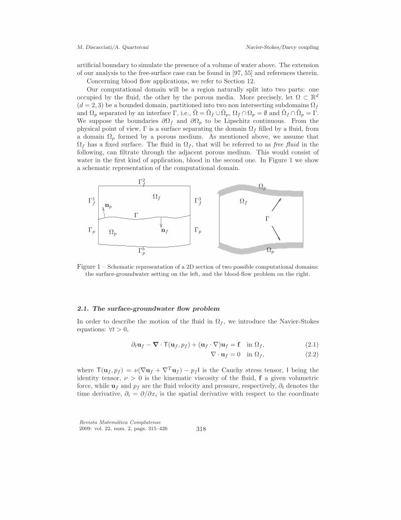
and Ωp separated by an interface Γ, i.e., Ω = Ωf ∪ Ωp, Ωf ∩Ωp = ∅ and Ωf ∩ Ωp = Γ.We suppose the boundaries ∂Ωf and ∂Ωp to be Lipschitz continuous. From thephysical point of view, Γ is a surface separating the domain Ωf filled by a fluid, froma domain Ωp formed by a porous medium. As mentioned above, we assume thatΩf has a fixed surface. The fluid in Ωf , that will be referred to as free fluid in thefollowing, can filtrate through the adjacent porous medium. This would consist ofwater in the first kind of application, blood in the second one. In Figure 1 we showa schematic representation of the computational domain.
Ωf
Ωpnf
npΓ1
f
Γ2f
Γ3f
Γp Γp
Γbp
Γ
Ωf
Ωp
Ωp
Γ
Figure 1 – Schematic representation of a 2D section of two possible computational domains:the surface-groundwater setting on the left, and the blood-flow problem on the right.
2.1. The surface-groundwater flow problem
In order to describe the motion of the fluid in Ωf , we introduce the Navier-Stokesequations: ∀t > 0,
∂tuf − ∇ · T(uf , pf ) + (uf · ∇)uf = f in Ωf , (2.1)
∇ · uf = 0 in Ωf , (2.2)
where T(uf , pf) = ν(∇uf + ∇T uf ) − pf I is the Cauchy stress tensor, I being theidentity tensor, ν > 0 is the kinematic viscosity of the fluid, f a given volumetricforce, while uf and pf are the fluid velocity and pressure, respectively, ∂t denotes thetime derivative, ∂i = ∂/∂xi is the spatial derivative with respect to the coordinate
Revista Matematica Complutense
2009: vol. 22, num. 2, pags. 315–426 318
M. Discacciati/A. Quarteroni Navier-Stokes/Darcy coupling
xi, while ∇ and ∇· are, respectively, the gradient and the divergence operator withrespect to the space coordinates. Moreover,
∇ · T =
d∑
j=1
∂jTij
i=1,...,d
.
Finally, we recall that
(v · ∇)w =
d∑
i=1
vi∂iw,
for all vector functions v = (v1, . . . , vd) and w = (w1, . . . , wd).
The filtration of an incompressible fluid through porous media is often describedusing Darcy’s law. The latter provides the simplest linear relation between velocityand pressure in porous media under the physically reasonable assumption that fluidflows are usually very slow and all the inertial (non-linear) terms may be neglected.
Groundwater flows could be treated microscopically by the laws of hydrodynamicsif the granular skeleton of the porous medium were a simple geometrical assembly ofunconnected tubes. However, the seepage path is tortuous and it branches into amultitude of tributaries. Darcy’s law avoids the insurmountable difficulties of thehydrodynamic microscopic picture by introducing a macroscopic concept. In fact, itconsiders a fictitious flow velocity, the Darcy velocity or specific discharge q througha given cross section of the porous medium, rather than the true velocity up withrespect to the porous matrix:
up =q
n, (2.3)
with n being the volumetric porosity, defined as the ratio between the volume of voidspace and the total volume of the porous medium.
This simplifying concept was introduced by the nature of Darcy’s experiment (see[50]) which only permitted the measurement of averaged hydraulic values from thepercolation of water through a column of horizontally stratified beds of sand in acylindrical pipe.
To introduce Darcy’s law, we define a scalar quantity ϕ called piezometric headwhich essentially represents the fluid pressure in Ωp:
ϕ = z +pp
g,
where z is the elevation from a reference level, accounting for the potential energy perunit weight of fluid, pp is the ratio between the fluid pressure in Ωp and its viscosityρf , and g is the gravity acceleration.
Then, Darcy’s law can be written as
q = −K∇ϕ, (2.4)
319Revista Matematica Complutense
2009: vol. 22, num. 2, pags. 315–426
M. Discacciati/A. Quarteroni Navier-Stokes/Darcy coupling
Table 1 – Typical values of hydraulic conductivity K.
K (m/s): 1 10−1 10−2 10−3 10−4 10−5 10−6 10−7 10−8 10−9 10−10 10−11 10−12
Permeability Pervious Semipervious ImperviousClean Clean sand or Very fine sand, silt,
Soils gravel sand and gravel loamPeat Stratified clay Unweathered clay
Good Breccia,Rocks Oil rocks Sandstone limestone, granite
dolomite
where K is a symmetric positive definite tensor K = (Kij)i,j=1,...,d, Kij ∈ L∞(Ωp),Kij > 0, Kij = Kji, called hydraulic conductivity tensor, which depends on theproperties of the fluid as well as on the characteristics of the porous medium. Infact, its components are proportional to nε2, where ε is the characteristic length ofthe pores; then, K ∝ ε2. The hydraulic conductivity K is therefore a macroscopicquantity characterizing porous media; in Table 1 we report some typical values thatit may assume (see [20]).
Finally, we notice that the hydraulic conductivity tensor K can be diagonalized byintroducing three mutually orthogonal axes called principal directions of anisotropy.In the following, we will always suppose that the principal axes are in the x, y andz directions so that the tensor will be considered diagonal: K = diag(K1,K2,K3).Moreover, let us denote K = K/n.
In conclusion, the motion of an incompressible fluid through a saturated porousmedium is described by the following equations:
up = −K∇ϕ in Ωp, (2.5)
∇ · up = 0 in Ωp. (2.6)
Extensions of Darcy’s law are given, e.g., by the Forchheimer’s or Brinkman’s equa-tions when the Reynolds number in Ωp is not small (see [67, 73, 95, 38]), or by morecomplicated models like Richards’ equations apt to describe saturated-unsaturatedfluid flows (see, e.g., [24] and references therein).
3. Interface conditions to couple surface and groundwater flows
We consider now the issue of finding effective coupling conditions across the interfaceΓ which separates the fluid flow in Ωf and the porous medium. This is a classical prob-lem which has been investigated from both a physical and a rigorous mathematicalpoint of view.
A mathematical difficulty arises from the fact that we need to couple two differentsystems of partial differential equations: Darcy equations (2.5)–(2.6) contain second
Revista Matematica Complutense
2009: vol. 22, num. 2, pags. 315–426 320

M. Discacciati/A. Quarteroni Navier-Stokes/Darcy coupling
order derivatives for the pressure and first order for the velocity, while in the Navier-Stokes system it is the opposite.
In the following, np and nf denote the unit outward normal vectors to the surfaces∂Ωp and ∂Ωf , respectively, and we have nf = −np on Γ. We suppose nf and np tobe regular enough. Moreover, we shall indicate n = nf for simplicity of notation, andby ∂n the partial derivative along n.
Three conditions are to be prescribed on Γ.
(i) The obvious condition to assign at a permeable interface is the continuity of thenormal velocity, which is a consequence of the incompressibility of both fluids:
uf · n = up · n on Γ.
(ii) Moreover, a suitable condition relating the pressures of the two fluids across Γhas to be prescribed.
(iii) Finally, in order to have a completely determined flow of the free fluid, we haveto specify a further condition on the tangential component of the fluid velocityat the interface.
Concerning the third point, a classically used condition for the free fluid is thevanishing of the tangential velocity at the interface, uf · τ j = 0 on Γ, where τ j
(j = 1, . . . , d − 1) are linear independent unit tangential vectors to the boundary Γ.However, this condition, which is correct in the case of a permeable surface, is notcompletely satisfactory for a permeable interface. (Let us remark that this conditionhas been used in [124] for blood flow simulations.) Beavers and Joseph proposed a newcondition postulating that the difference between the slip velocity of the free fluid andthe tangential component of the velocity through the porous medium is proportionalto the shear rate of the free fluid (see [21]). They verified this law experimentally andfound that the proportionality constant depends linearly on the square root of thepermeability. Precisely, the coupling condition that they advocated reads:
τ j · ∂nuf =αBJ√
K(uf − up) · τ j on Γ, (3.1)
where αBJ is a dimensionless constant which depends only on the structure of theporous medium.
This experimentally found coupling condition was further studied by Saffman (see[115]) who pointed out that the velocity up was much smaller than the other quantitiesappearing in equation (3.1) and that, in fact, it could be dropped. The new proposedinterface condition reads therefore
τ j · ∂nuf =αBJ√
Kuf · τ j +O(
√K) on Γ. (3.2)
321Revista Matematica Complutense
2009: vol. 22, num. 2, pags. 315–426
M. Discacciati/A. Quarteroni Navier-Stokes/Darcy coupling
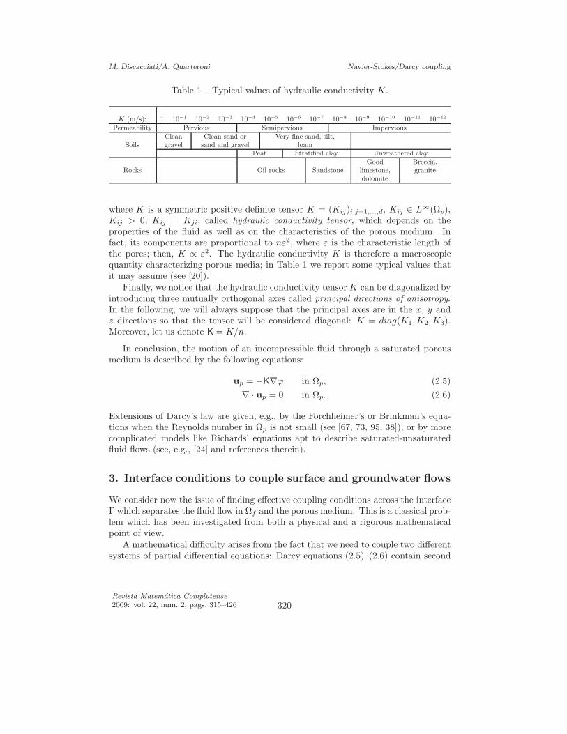
This problem was later reconsidered in [66] and [89] using an asymptotic expansionargument and distinguishing two cases. First, the authors considered the case of apressure gradient on the side of the porous medium normal to the interface (seeFigure 2, left); they found that the flow is balanced on both sides of the interfaceand that the velocities across Γ are of the same order. Then, using an asymptoticexpansion, they obtained the following interface laws:
uf · n = up · n, pf = const on Γ.
ΓΓ
ΩfΩf
ufuf
ΩpΩp
∇pf∇pf
∇pp∇pp
Figure 2 – Two configurations for the pressure gradient: on the left, normal to theinterface Γ; on the right, oblique to Γ.
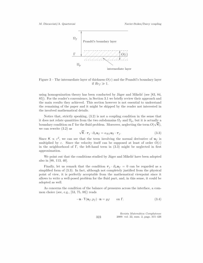
Secondly, they studied the case of pressure gradient not normal (oblique) to theinterface (see Figure 2, right). In this case, it is found in [66] and [89] that thevelocity uf is much larger than the filtration velocity in the porous body and, in thefirst approximation, the flow around the porous medium is the same as if the bodywere impervious. Then, investigation in the vicinity of Γ lead to the existence ofan intermediate layer, of characteristic thickness ε (the representative length of theporous matrix), which allows the asymptotic matching of the free fluid with the flowin the porous body. The free fluid contains a Prandtl’s type boundary layer near Γ forlarge Reynolds number Ref (see Figure 3). We recall that Ref = LfUf/ν, Lf beinga characteristic length of the domain Ωf and Uf a characteristic velocity of the fluid.The conclusion drawn is that a suitable interface condition across Γ is the continuityof the pressure.
In practice, however, when solving the effective equations, the boundary conditionson Γ are not enough to guarantee the well-posedness of the fluid problem, as opposedto the interface equations of Beavers and Joseph that yield a well-posed problem inthe free fluid domain.
A first attempt toward an analytical study of the interface conditions between afree fluid and a porous medium can be found in [105]; a mathematical investigation
Revista Matematica Complutense
2009: vol. 22, num. 2, pags. 315–426 322
M. Discacciati/A. Quarteroni Navier-Stokes/Darcy coupling
intermediate layer
Prandtl’s boundary layer
O(ε)
Ωf
Ωp
Γ
Figure 3 – The intermediate layer of thickness O(ε) and the Prandtl’s boundary layerif Ref ≫ 1.
using homogenization theory has been conducted by Jager and Mikelic (see [83, 84,85]). For the reader’s convenience, in Section 3.1 we briefly review their approach andthe main results they achieved. This section however is not essential to understandthe remaining of the paper and it might be skipped by the reader not interested inthe involved mathematical details.
Notice that, strictly speaking, (3.2) is not a coupling condition in the sense thatit does not relate quantities from the two subdomains Ωf and Ωp, but it is actually a
boundary condition on Γ for the fluid problem. Moreover, neglecting the term O(√
K),we can rewrite (3.2) as √
K · τ j · ∂nuf = αBJuf · τ j . (3.3)
Since K ∝ ε2, we can see that the term involving the normal derivative of uf ismultiplied by ε. Since the velocity itself can be supposed at least of order O(ε)in the neighborhood of Γ, the left-hand term in (3.3) might be neglected in firstapproximation.
We point out that the conditions studied by Jager and Mikelic have been adoptedalso in [88, 113, 40].
Finally, let us remark that the condition τ j · ∂nuf = 0 can be regarded as asimplified form of (3.3). In fact, although not completely justified from the physicalpoint of view, it is perfectly acceptable from the mathematical viewpoint since itallows to write a well-posed problem for the fluid part, and, in this sense, it could beadopted as well.
As concerns the condition of the balance of pressures across the interface, a com-mon choice (see, e.g., [53, 75, 88]) reads
−n · T(uf , pf ) · n = gϕ on Γ. (3.4)
323Revista Matematica Complutense
2009: vol. 22, num. 2, pags. 315–426
M. Discacciati/A. Quarteroni Navier-Stokes/Darcy coupling
This condition, which actually allows the pressure to be discontinuous across Γ, iswell-suited for the analysis of the coupled fluid-groundwater flow problem. Indeed,it can be naturally incorporated in its weak formulation as it is a Neumann-typeboundary condition on Γ for the Navier-Stokes equations (2.1)–(2.2). We will show itin details in Section 4. Let us notice that if one adopted the divergence form of theNavier-Stokes momentum equation:
∂tuf − ∇ · T(uf , pf ) + ∇ · (uf uTf ) = f in Ωf ,
then, (3.4) should be replaced by the following one (see [75])
−n · T(uf , pf ) · n +1
2(uf · uf ) = gϕ on Γ, (3.5)
that is, pressure pf in (3.4) has to be replaced by the total pressure pf + 12 |uf |2 in
(3.5).
At the end of this section, let us write the coupled Navier-Stokes/Darcy model:
∂tuf − ∇ · T(uf , pf ) + (uf · ∇)uf = f in Ωf ,
∇ · uf = 0 in Ωf , (3.6)
up = −K∇ϕ in Ωp, (3.7)
∇ · up = 0 in Ωp, (3.8)
uf · n = up · n on Γ, (3.9)
−n · T(uf , pf ) · n = gϕ on Γ, (3.10)ναBJ√
Kuf · τ j − τ j · T(uf , pf ) · n = 0 on Γ. (3.11)
Moreover, let us point out that using Darcy’s law we can rewrite the system (2.5)–(2.6) as an elliptic equation for the scalar unknown ϕ:
−∇ · (K∇ϕ) = 0 in Ωp. (3.12)
In this case, the differential formulation of the coupled Navier-Stokes/Darcy prob-lem becomes:
∂tuf − ∇ · T(uf , pf ) + (uf · ∇)uf = f in Ωf , (3.13)
∇ · uf = 0 in Ωf (3.14)
−∇ · (K∇ϕ) = 0 in Ωp, (3.15)
with the interface conditions on Γ:
uf · n = −K∂nϕ, (3.16)
−n · T(uf , pf ) · n = gϕ, (3.17)ναBJ√
Kuf · τ j − τ j · T(uf , pf ) · n = 0. (3.18)
Revista Matematica Complutense
2009: vol. 22, num. 2, pags. 315–426 324
M. Discacciati/A. Quarteroni Navier-Stokes/Darcy coupling
The global problem is then non-linear. A linearization can be obtained by replacingthe Navier-Stokes momentum equation (3.13) with the Stokes one:
∂tuf − ∇ · T(uf , pf) = f in Ωf , (3.19)
i.e., dropping the non-linear convective terms. This replacement is justified whenthe Reynolds number Ref of the fluid is low, i.e., in case of slow motion of fluidswith high viscosity. This linearized problem is also interesting since a steady Stokesproblem can be generated when considering a semi-implicit time advancement of theNavier-Stokes equations where all terms but the non-linear convective one have beendealt with implicitly.
3.1. Mathematical derivation of the law of Beavers, Joseph and Saffmanvia homogenization
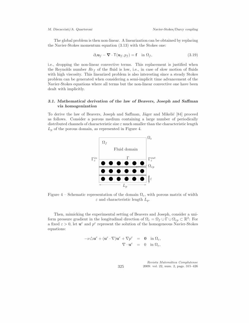
To derive the law of Beavers, Joseph and Saffman, Jager and Mikelic [84] proceedas follows. Consider a porous medium containing a large number of periodicallydistributed channels of characteristic size εmuch smaller than the characteristic lengthLp of the porous domain, as represented in Figure 4.
Ωf
Ωεp
Γ
ε
Lp
Γinε Γout
ε
Fluid domain
Ωε
Figure 4 – Schematic representation of the domain Ωε, with porous matrix of widthε and characteristic length Lp.
Then, mimicking the experimental setting of Beavers and Joseph, consider a uni-form pressure gradient in the longitudinal direction of Ωε = Ωf ∪ Γ ∪ Ωεp ⊂ R
2: Fora fixed ε > 0, let uε and pε represent the solution of the homogeneous Navier-Stokesequations:
−νuε + (uε · ∇)uε + ∇pε = 0 in Ωε,
∇ · uε = 0 in Ωε,
325Revista Matematica Complutense
2009: vol. 22, num. 2, pags. 315–426
M. Discacciati/A. Quarteroni Navier-Stokes/Darcy coupling
withpε = p0 on Γin
ε and pε = pb on Γoutε ,
and homogeneous boundary conditions on the velocity (see [84]).
Remark 3.1. Adopting the Navier-Stokes equations not only in Ωf but also in Ωεp
is motivated by the fact that Darcy’s law can be obtained from the (Navier-)Stokesequations through homogenization, at least in the interior of Ωεp. A proof can befound, e.g., in [117] where it is shown that the sequences of functions (depending onε) uε and pε in Ωεp which satisfy the Stokes equations
−uε + ∇pε = f in Ωεp,
∇ · uε = 0 in Ωεp,
uε = 0 on ∂Ωεp,
tend to the asymptotic velocity u0p and pressure p0
p:
uε
ε2 u0
p weakly in L2(Ωp),
pε → p0p strongly in L2(Ωp),
where u0p and p0
p satisfy the boundary value problem
u0p = −K(∇p0
p − f) in Ωp,
∇ · u0p = 0 in Ωp,
u0p · np = 0 on ∂Ωp.
From the convergence proof it can be seen that K ∝ ε2/ν.
Jager and Mikelic proved that, consistently with the considerations by Ene andSanchez-Palencia, the velocity field is of order O(1) in Ωf , of order O(ε2) in Ωεp,and that there is a boundary layer of thickness O(ε) for the velocity at the interface,while the pressure fields are of order O(1) in both media. In particular, the effectivevelocity field in Ωf is described by the solution u0
f of Stokes equations with the no-slip
condition u0f = 0 on Γ, giving an L2-approximation of order O(ε) for the velocity uε.
However, since this approximation is too rough as it cannot account for the velocityin the porous medium which is O(ε2), in [84] higher order terms in ε are consideredfor the velocity, introducing a boundary layer problem across Γ whose solution decaysexponentially away from Γ and which accounts for the shear effects near the interface.
This correction yields the following interface conditions for the macroscale prob-lem:
uf · τ j − εCbl1 τ j · ∂nuf = 0 on Γ (3.20)
andpp = pf − νCbl
2 n · ∂nuf on Γ, (3.21)
Revista Matematica Complutense
2009: vol. 22, num. 2, pags. 315–426 326
M. Discacciati/A. Quarteroni Navier-Stokes/Darcy coupling
where Cbl1 and Cbl
2 (bl stands for boundary layer) are two suitable positive constants.Finally, the following estimates hold (see [84]):
‖∇(uε − uf )‖L1(Ωf ) ≤ Cε| log ε|,‖uε − uf‖H1/2−γ(Ωf ) ≤ C′ε3/2| log ε|,
where 0 < γ < 1/2 (the log term being due to the presence of corners in the domain).Notice that (3.20) is exactly Saffman’s modification of Beavers and Joseph’s law
with√
K/αBJ = εCbl1 , while condition (3.21) shows that, somehow contrary to intu-
ition, the effective pressure in the system free flow/porous medium is not necessar-ily continuous and, therefore this contradicts the continuity assumption of Sanchez-Palencia [66, 89].
As for the quantitative value of the constants Cbl1 , Cbl
2 , the latter have been com-puted for some configurations of porous media; on the base of the results reported in[85], it may be speculated that Cbl
1 , Cbl2 ∼ 1. In the computations that are presented
in this paper we have actually set Cbl1 = αBJ and Cbl
2 = 1.
4. Weak formulation and analysis
From now on, we focus on the coupled problem (3.13)–(3.18), however we considerthe steady Navier-Stokes problem by dropping the time-derivative in the momentumequation (3.13):
−∇ · T(uf , pf) + (uf · ∇)uf = f in Ωf . (4.1)
A similar kind of “steady” problem can be found when using an implicit time-advancing scheme on the time-dependent problem (3.13). In that case, however,an extra reaction term αuf would show up on the left-hand side of (4.1), where thepositive coefficient α plays the role of inverse of the time-step. This reaction termwould not affect our forthcoming analysis, though.
Let us discuss now about possible boundary conditions to be prescribed on theexternal boundary of Ωf and Ωp.
We split the boundaries ∂Ωf and ∂Ωp of Ωf and Ωp as ∂Ωf = Γ ∪ Γ1f ∪ Γ2
f ∪ Γ3f
and ∂Ωp = Γ ∪ Γp ∪ Γbp, as shown in Figure 1, left.
For the Darcy equation we assign the piezometric head ϕ = ϕp on Γp; moreover,we require that the normal component of the velocity vanishes on the bottom surface,that is, up · np = 0 on Γb
p.For the Navier-Stokes problem, several combinations of boundary conditions could
be considered, representing different kinds of flow problems; we indicate some of them.A first possibility is to assign the velocity vector uf = 0 on Γ1
f ∪Γ3f and a natural
boundary condition T(uf , pf ) · nf = g on Γ2f (a fictitious boundary), where g is a
given vector function, representing the flux across Γ2f of the fluid column standing
above.
327Revista Matematica Complutense
2009: vol. 22, num. 2, pags. 315–426
M. Discacciati/A. Quarteroni Navier-Stokes/Darcy coupling
Alternatively, we can prescribe a non-null inflow uf = uin on the left-hand bound-ary Γ1
f , a slip condition uf · nf = 0 and τ i · T(uf , pf) · nf = 0 on Γ2f and an outflow
condition T(uf , pf ) · nf = 0 on the right-hand boundary Γ3f which describes a free
outflow or a free stress at the outflow boundary.A third possibility consists of assigning again a non-null inflow uf = uin on the
left-hand boundary Γ1f and a no-slip condition uf = 0 on the remaining boundary
Γ2f ∪ Γ3
f .Our analysis considers the last choice we have indicated, but it can be modified to
accommodate the other boundary conditions as well. From now on, we denote Γ1f as
Γinf (standing for Γinflow
f ) and the remaining boundary Γ2f ∪ Γ3
f simply by Γf . Thus,we supplement the coupled problem (3.13)–(3.18) with the boundary conditions:
uf = uin on Γinf , (4.2)
uf = 0 on Γf ,
ϕ = ϕp on Γp,
K ∂nϕ = 0 on Γbp. (4.3)
We introduce the following functional spaces:
HΓf= v ∈ H1(Ωf ) : v = 0 on Γf,
HΓf∪Γinf
= v ∈ HΓf: v = 0 on Γin
f , Hf = (HΓf∪Γinf
)d,
H0f = v ∈ Hf : v · nf = 0 on Γ,fHf = v ∈ (H1(Ωf ))d : v = 0 on Γf ∪ Γ,
Q = L2(Ωf ), Q0 = q ∈ Q :∫
Ωfq = 0,
Hp = ψ ∈ H1(Ωp) : ψ = 0 on Γp, H0p = ψ ∈ Hp : ψ = 0 on Γ.
We denote by | · |1 and ‖ · ‖1 the H1–seminorm and norm, respectively, and by‖ · ‖0 the L2–norm; it will always be clear form the context whether we are referringto spaces on Ωf or Ωp.
The space W = Hf ×Hp is a Hilbert space with norm
‖w‖W =(
‖w‖21 + ‖ψ‖2
1
)1/2 ∀w = (w, ψ) ∈W.
Finally, we consider on Γ the trace space Λ = H1/200 (Γ) and denote its norm by ‖ · ‖Λ
(see [90]).
We introduce a continuous extension operator
Ef : (H1/2(Γinf ))d →fHf . (4.4)
Then ∀uin ∈ (H1/200 (Γin
f ))d we can construct a vector function Efuin ∈fHf such thatEfuin|Γin
f= uin.
Revista Matematica Complutense
2009: vol. 22, num. 2, pags. 315–426 328

M. Discacciati/A. Quarteroni Navier-Stokes/Darcy coupling
Remark 4.1. Alternatively, we could consider a divergence free extension ÜEfuin of uin.To this aim, let Efuin ∈ (HΓf
)d such that Efuin = uin on Γinf . Then, we construct a
function win which is the solution of the following problem: find win ∈ Hf such thatfor all q ∈ Q
−∫
Ωf
q∇ · win =
∫
Ωf
q∇ · (Efuin) . (4.5)
The solvability of (4.5) is guaranteed by the inf-sup condition: there exists a constantβ∗ > 0 such that
∀q ∈ Q ∃v ∈ Hf , v 6= 0 : −∫
Ωf
q∇ · v ≥ β‖v‖1‖q‖0 (4.6)
(see, e.g., [110, pages 157–158]). Finally, we indicate by ÜEfuin = Efui + win the
divergence-free extension of uin. We remark that ÜEfuin = uin on Γinf , ÜEfuin = 0 on
Γf and that, thanks to (4.5), it holds
∫
Ωf
q∇ · (ÜEfuin) = 0, ∀q ∈ Q .
We point out that the extension ÜEfuin cannot satisfy the additional constraint ÜEfuin ·nf = 0 on Γ, except for the special case of uin such that
∫
Γinf
uin · nf = 0.
We introduce another continuous extension operator:
Ep : H1/2(Γbp) → H1(Ωp) such that Epϕp = 0 on Γ.
Then, for all ϕ ∈ H1(Ωp) we define the function ϕ0 = ϕ− Epϕp.
Finally, we define the following bilinear forms:
af (v,w) =
∫
Ωf
ν
2(∇v + ∇Tv) · (∇w + ∇T w) ∀v,w ∈ (H1(Ωf ))d,
bf(v, q) = −∫
Ωf
q∇ · v ∀v ∈ (H1(Ωf ))d, ∀q ∈ Q,
ap(ϕ, ψ) =
∫
Ωp
∇ψ · K∇ϕ ∀ϕ, ψ ∈ H1(Ωp) ,
and, for all v,w, z ∈ (H1(Ωf ))d, the trilinear form
cf (w; z,v) =
∫
Ωf
[(w · ∇)z] · v =
d∑
i,j=1
∫
Ωf
wj∂zi
∂xjvi .
329Revista Matematica Complutense
2009: vol. 22, num. 2, pags. 315–426
M. Discacciati/A. Quarteroni Navier-Stokes/Darcy coupling
Now, if we multiply (4.1) by v ∈ Hf and integrate by parts we obtain
af (uf ,v) + cf (uf ;uf ,v) + bf (v, pf ) −∫
Γ
n · T(uf , pf)v =
∫
Ωf
f v .
Notice that we can write
−∫
Γ
n · T(uf , pf )v = −∫
Γ
[n · T(uf , pf ) · n]v · n−∫
Γ
d−1∑
j=1
[n · T(uf , pf ) · τ j ]v · τ j ,
so that we can incorporate in weak form the interface conditions (3.17) and (3.18) asfollows:
−∫
Γ
n · T(uf , pf )v =
∫
Γ
gϕ(v · n) +
∫
Γ
d−1∑
j=1
ναBJ√K
(uf · τ j)(v · τ j) .
Finally, we consider the lifting Efuin of the boundary datum and we split uf =u0
f + Efuin with u0f ∈ Hf ; we recall that Efuin = 0 on Γ and we get
af (u0f ,v) + cf (u0
f + Efuin;u0f + Efuin,v) + bf (v, pf )
+
∫
Γ
gϕ(v · n) +
∫
Γ
d−1∑
j=1
ναBJ√K
(uf · τ j)(v · τ j) =
∫
Ωf
f v − af (Efuin,v). (4.7)
From (3.14) we find
bf (u0f , q) = −bf(Efuin, q) ∀q ∈ Q. (4.8)
On the other hand, if we multiply (3.15) by ψ ∈ Hp and integrate by parts we get
ap(ϕ, ψ) +
∫
Γ
K∂nϕψ = 0 .
Now we incorporate the interface condition (3.16) in weak form as
ap(ϕ, ψ) −∫
Γ
(uf · n)ψ = 0,
and, considering the splitting ϕ = ϕ0 + Epϕp we obtain
ap(ϕ0, ψ) −∫
Γ
(uf · n)ψ = −ap(Epϕp, ψ). (4.9)
Revista Matematica Complutense
2009: vol. 22, num. 2, pags. 315–426 330
M. Discacciati/A. Quarteroni Navier-Stokes/Darcy coupling
We multiply (4.9) by g and sum to (4.7) and (4.8). Then, we define
A(v, w) = af (v,w) + g ap(ϕ, ψ) +
∫
Γ
g ϕ(w · n) −∫
Γ
g ψ(v · n)
+
∫
Γ
d−1∑
j=1
ναBJ√K
(w · τ j)(v · τ j),
C(v;w, u) = cf (v;w,u),
B(w, q) = bf (w, q),
for all v = (v, ϕ), w = (w, ψ), u = (u, ξ) ∈ W , q ∈ Q. Finally, we define the followinglinear functionals:
〈F , w〉 =
∫
Ωf
f w − af (Efuin,w) − g ap(Epϕp, ψ), (4.10)
〈G, q〉 = −bf(Efuin, q),
for all w = (w, ψ) ∈W , q ∈ Q.Adopting these notations, the weak formulation of the coupled Navier-Stokes/Dar-
cy problem reads:
find u = (u0f , ϕ0) ∈W , pf ∈ Q such that
A(u, v) + C(u+ u∗;u+ u∗, v) + B(v, pf) = 〈F , v〉 ∀v = (v, ψ) ∈ W, (4.11)
B(u, q) = 〈G, q〉 ∀q ∈ Q, (4.12)
with u∗ = (Efuin, 0) ∈fHf ×H1(Ωp).
Remark that the interface conditions (3.16)–(3.18) have been incorporated in theabove weak model as natural conditions on Γ. In particular, (3.17) and (3.18) arenatural conditions for the Navier-Stokes problem, while (3.16) becomes a naturalcondition for Darcy’s problem.
4.1. Analysis of the linear coupled Stokes/Darcy problem
In this section we consider the analysis of the coupled problem where we replacethe Navier-Stokes equations by the Stokes equations, i.e., we neglect the non-linearconvective term. The weak formulation of the Stokes/Darcy problem can be obtainedstraightforwardly from (4.11)–(4.12) dropping the trilinear form C(·; ·, ·). Thus, wehave:
find u = (u0f , ϕ0) ∈W , pf ∈ Q such that
A(u, v) + B(v, pf ) = 〈F , v〉 ∀v = (v, ψ) ∈W, (4.13)
B(u, q) = 〈G, q〉 ∀q ∈ Q. (4.14)
331Revista Matematica Complutense
2009: vol. 22, num. 2, pags. 315–426
M. Discacciati/A. Quarteroni Navier-Stokes/Darcy coupling
In order to prove existence and uniqueness for the solution of the Stokes/Darcycoupled problem, we introduce some preliminary results on the properties of thebilinear forms A and B and of the functional F .
Lemma 4.2. The following results hold:
(i) A(·, ·) is continuous and coercive on W and, in particular, it is coercive on thekernel of B
W 0 = v ∈ W : B(v, q) = 0, ∀q ∈ Q ;
(ii) B(·, ·) is continuous on W×Q and satisfies the following inf-sup condition: thereexists a positive constant β > 0 such that
∀q ∈ Q ∃w ∈W, w 6= (0, 0) : B(w, q) ≥ β‖w‖W ‖q‖0. (4.15)
(iii) F is a continuous linear functional on W .
(iv) G is a continuous linear functional on Q.
Proof.(i) The following trace inequalities hold (see [90]):
∃Cf > 0 such that ‖v|Γ‖Λ ≤ Cf‖v‖1 ∀v ∈ Hf ; (4.16)
∃Cp > 0 such that ‖ψ|Γ‖Λ ≤ Cp‖ψ‖1 ∀ψ ∈ Hp. (4.17)
Thanks to the Cauchy–Schwarz inequality and the above trace inequalities the conti-nuity of A(., .) follows:
|A(v, w)| ≤ 2ν‖v‖1‖w‖1 + gmaxj
‖Kj‖∞‖ψ‖1‖ϕ‖1
+gCfCp‖ϕ‖1‖w‖1 + gCfCp‖ψ‖1‖v‖1
+(d− 1)(ναBJ/√
K)C2f‖v‖1‖w‖1.
We defineγ = maxγ1, γ2, (4.18)
where
γ1 = max2ν + (d− 1)C2f (ναBJ/
√K), gCfCp,
γ2 = maxgmaxj
‖Kj‖∞, gCfCp,
so that|A(v, w)| ≤ γ(‖v‖1 + ‖ϕ‖1)(‖w‖1 + ‖ψ‖1) ≤ 2γ‖v‖W ‖w‖W ,
which follows from the inequality (x + y) ≤√
2(x2 + y2)1/2, ∀x, y ∈ R+.
Revista Matematica Complutense
2009: vol. 22, num. 2, pags. 315–426 332
M. Discacciati/A. Quarteroni Navier-Stokes/Darcy coupling
The coercivity is a consequence of the Korn inequality (see, e.g., [51, page 416] or[110, page 149]): ∀v = (v1, . . . , vd) ∈ Hf
∃κf > 0 such that
∫
Ωf
d∑
j,l=1
(∂lvj + ∂jvl)2 ≥ κf‖v‖2
1 , (4.19)
and the Poincare inequality (see [90] and [109, page 11]):
∃CΩp > 0 such that ‖ψ‖20 ≤ CΩp‖∇ψ‖2
0 ∀ψ ∈ Hp .
In fact we have for all v = (v, ϕ) ∈W ,
A(v, v) = af (v,v) + g ap(ϕ,ϕ) +
∫
Γ
d−1∑
j
ναBJ√K
(v · τ j)2
≥ af (v,v) + g ap(ϕ,ϕ)
≥ νκf‖v‖21 + gmK min(1, C−1
Ωp)‖ϕ‖2
1 ≥ α‖v‖2W ,
whereα = minνκf , gmK min(1, C−1
Ωp), (4.20)
with mK = mini=1,...,d infx∈Ωp Ki(x) > 0. Finally, since W 0 ⊂W , the thesis follows.
(ii) Concerning the continuity, thanks to the Cauchy–Schwarz inequality, we have
|B(w, q)| ≤ ‖q‖0‖w‖W ∀w ∈ W, q ∈ Q.
Moreover, thanks to (4.6), there exists a constant β∗ > 0 such that
∀q ∈ Q ∃w ∈ Hf , w 6= 0 : −∫
Ωf
q∇ · w ≥ β∗‖w‖1‖q‖0.
Then, considering w = (w, 0) ∈ Hf ×Hp, the result follows with β = β∗ > 0.
(iii) Thanks to the Cauchy-Schwarz inequality and the continuity of the extensionoperators Ef and Ep, whose continuity constants are denoted hereafter by C1 andC2, respectively, we have
|〈F , w〉| ≤ ‖f‖0‖w‖1 + νC1‖uin‖H1/2(Γinf )‖w‖1
+gmaxj
‖Kj‖∞C2‖ψ‖1‖ϕ‖H1/2(Γbp)
≤ CF (‖w‖1 + ‖ϕ‖1) ≤√
2CF‖w‖W ,
where
CF = max‖f‖0 + C1ν‖uin‖H1/2(Γinf ), gC2 max
j‖Kj‖∞‖ϕp‖H1/2(Γb
p). (4.21)
333Revista Matematica Complutense
2009: vol. 22, num. 2, pags. 315–426
M. Discacciati/A. Quarteroni Navier-Stokes/Darcy coupling
(iv) The continuity of the functional G follows from the Cauchy-Schwarz inequalityand from the continuity of the extension operator Ef ; in fact it holds:
|〈G, q〉| ≤ CG‖q‖0, (4.22)
with CG = C1‖uin‖H1/2(Γinf ).
We can now prove the main result of this Section.
Proposition 4.3. The Stokes/Darcy coupled problem (4.13)–(4.14) admits a uniquesolution (u0
f , pf , ϕ0) ∈ Hf ×Q×Hp which satisfies the following a-priori estimates:
‖(u0f , ϕ0)‖W ≤ 1
α
(√2CF +
α+ 2γ
βCG
)
,
‖pf‖0 ≤ 1
β
[(
1 +2γ
α
)√2CF +
2γ(α+ 2γ)
αβCG
]
,
where β, γ, α, CF and CG are the constants defined in (4.15), (4.18), (4.20), (4.21)and (4.22), respectively.
Proof. This is a straightforward consequence of the existence and uniqueness theoremof Brezzi (see [29, 33]), whose hypotheses are satisfied thanks to Lemma 4.2.
Remark 4.4. From Proposition 4.3 it follows in particular that −K∂nϕ|Γ ∈ Λ, sinceuf · n|Γ ∈ Λ. Then, on Γ, ϕ has a higher regularity than one might have expected.
4.2. Mixed formulation of Darcy’s equation
In the analysis presented so far we have chosen to rewrite Darcy’s equation in formof the Poisson problem (3.15). Should we keep the mixed formulation (2.5)–(2.6) awell-posedness analysis can be developed as well; we refer to [88]. In this reference aStokes/Darcy coupling analogous to the one of Section 4.1 is considered. Still adoptingthe interface conditions proposed by Jager and Mikelic, a mixed form of Darcy’sequations is used; the coupling is realized via Lagrange multipliers. In particular, thefollowing Lagrange multiplier
ℓ ∈ Λ, ℓ = −n · T(uf , pf ) · n = pp on Γ,
and the dual pairing
bΓ : (Hf ×X2) × Λ → R, bΓ(v, ℓ) = 〈v1 · n + v2 · n, ℓ〉
are introduced, where X2 is a suitable subspace of H(div; Ωp) accounting for theboundary conditions and where we have denoted v = (v1,v2).
Revista Matematica Complutense
2009: vol. 22, num. 2, pags. 315–426 334
M. Discacciati/A. Quarteroni Navier-Stokes/Darcy coupling
Then, existence and uniqueness of the solution of the following global mixed problemis proved:
find u = (uf ,up) ∈ Hf ×X2, p = (pf , pp) ∈M , ℓ ∈ Λ:
a(u, v) + b(v, p) + bΓ(v, ℓ) = f(v) ∀v ∈ Hf ×X2, (4.23)
b(u, q) = g(q) ∀q ∈M, (4.24)
bΓ(u, σ) = 0 ∀σ ∈ Λ, f (4.25)
with
a(u, v) = af (uf ,vf ) +
∫
Γ
d−1∑
j=1
ναBJ√K
(uf · τ j)(vf · τ j) +
∫
Ωp
K−1up vp,
b(v, p) = bf (vf , pf ) −∫
Ωp
pp∇ · vp,
where f , g are suitably defined linear continuous functionals. Finally, M is a subspaceof Q× L2(Ωp).
If the computational domain is such that Γ∩∂Ω = ∅, i.e., if the porous medium isentirely enclosed in the fluid region, then (4.23)–(4.25) can be equivalently restatedon the subspace of Hf ×X2 with trace continuous normal velocities:
v ∈ Hf ×X2 : bΓ(v, σ) = 0, ∀σ ∈ Λ ⊂ Hf ×X2.
A study of the Stokes/Darcy problem in mixed form can also be found in [69, 72].In particular, in [69] different possible weak formulations are studied.
4.3. Time-dependent Stokes/Darcy model
The analysis of a time-dependent Stokes/Darcy system has been recently carried outin [43]. In particular, equation (2.6) has been replaced by the saturated flow model:
s∂tϕ+ ∇ · up = 0 in Ωp, (4.26)
where s denotes the mass storativity coefficient which gives the mass of water added tostorage (or released from it) in the porous medium depending on the rise (or decline)of the potential ϕ. Combining (4.26) and (2.5), the following time-dependent equationfor the piezometric head is obtained:
s∂tϕ−∇ · (K∇ϕ) = 0 in Ωp.
The Beavers-Joseph condition without Saffman’s simplification is used for the cou-pling, i.e.,
−τ j · T(uf , pf) · n =ναBJ√K
(uf − up) · τ j on Γ.
335Revista Matematica Complutense
2009: vol. 22, num. 2, pags. 315–426
M. Discacciati/A. Quarteroni Navier-Stokes/Darcy coupling
Consider now the bilinear form Aη(v, w) : W ×W → R,
Aη(v, w) = af (v,w) +η
sap(ϕ, ψ) +
∫
Γ
g ϕ(w · n) − η
s
∫
Γ
ψ(v · n)
+
∫
Γ
d−1∑
j=1
ναBJ√K
((v + K∇ϕ) · τ j)(w · τ j),
for all v = (v, ϕ), w = (w, ψ) ∈ W , where η is a suitable scaling parameter, and thefollowing duality pairing associated with the time derivative:
〈vt, w〉 = 〈∂tv,w〉 + η〈∂tϕ, ψ〉.
Then, we can write the weak form of the coupled time-dependent Stokes/Darcy prob-lem as:
find u = (uf , ϕ) and pf such that
〈ut, v〉 + Aη(u, v) + B(v, pf ) = 〈fF , v〉 ∀v = (v, ψ) ∈W,B(u, q) = 0 ∀q ∈ Q,
where fF is a linear continuous functional defined similarly to (4.10) and B is thebilinear form (4.10).
The problem is studied firstly in the steady case showing its well-posedness forsmall enough values of the coefficient αBJ . Then, a backward-Euler discretization intime is introduced and the convergence to the continuous solution as the time steptends to zero is proved. Finally, the convergence of the fully discretized system isguaranteed.
These results rely on the choice of a suitably large parameter η. Notice that thechoice of a large rescaling parameter η makes sense since the flow in porous mediaevolves on a relatively slow time scale compared to that of the flow in the conduit,and the re-scaling essentially brings them to the same time scale.
5. Multi-domain formulation of the Stokes/Darcy problem
Another possible approach to study the Navier-Stokes/Darcy problem is to exploit itsnaturally decoupled structure keeping separated the fluid and the porous media partsand exchanging information between surface and groundwater flows only throughboundary conditions at the interface. From the computational point of view, thisstrategy is useful at the stage of setting up effective methods to solve the problemnumerically. As we shall illustrate in Section 7, a discretization of this problem using,e.g., finite elements leads to a large sparse ill-conditioned linear system which requiresa suitable preconditioning strategy to be solved. We would like to exploit the intrinsicdecoupled structure of the problem at hand to design an iterative procedure requiring
Revista Matematica Complutense
2009: vol. 22, num. 2, pags. 315–426 336
M. Discacciati/A. Quarteroni Navier-Stokes/Darcy coupling
at each step to compute independently the solution of the fluid and of the groundwaterproblems.
Therefore, in the next sections we shall apply a domain decomposition techniqueat the differential level to study the Navier-Stokes/Darcy coupled problem. Our aimwill be to introduce and analyze a generalized Steklov-Poincare interface equation (see[110]) associated to our problem, in order to reformulate it solely in terms of interfaceunknowns. This re-interpretation will be crucial to set up iterative procedures betweenthe subdomains Ωf and Ωp, that will be later replicated at the discrete level.
In this section we start by considering the Stokes/Darcy problem, while Section 6concerns the Navier-Stokes/Darcy coupling.
The Stokes/Darcy problem can be rewritten in a multi-domain formulation and,in particular, we prove the following result.
Proposition 5.1. Let Λ be the space of traces introduced in Section 4. Problem(4.11)–(4.12) can be reformulated in an equivalent way as follows:
find u0f ∈ Hf , pf ∈ Q, ϕ0 ∈ Hp such that
af(u0f + Efuin,w) + bf (w, pf )
+
∫
Γ
d−1∑
j=1
ναBJ√K
(u0f · τ j)(R1µ · τ j) =
∫
Ωf
f w ∀w ∈ H0f , (5.1)
bf(u0f + Efuin, q) = 0 ∀q ∈ Q, (5.2)
ap(ϕ0 + Epϕp, ψ) = 0 ∀ψ ∈ H0p , (5.3)
∫
Γ
(u0f · n)µ = ap(ϕ0 + Epϕp, R2µ) ∀µ ∈ Λ, (5.4)
∫
Γ
gϕ0µ =
∫
Ωf
f (R1µ) − af (u0f + Efuin, R1µ) − bf(R1µ, pf )
−∫
Γ
d−1∑
j=1
ναBJ√K
(u0f · τ j)(R1µ · τ j) ∀µ ∈ Λ, (5.5)
where R1 is any possible extension operator from Λ to Hf , i.e., a continuous operatorfrom Λ to Hf such that (R1µ) · n = µ on Γ for all µ ∈ Λ, and R2 is any possiblecontinuous extension operator from H1/2(Γ) to Hp such that R2µ = µ on Γ for allµ ∈ H1/2(Γ).
Proof. Let (u, p) ∈ W ×Q be the solution of (4.11)–(4.12). Considering in (4.11) astest functions (w,ψ) ∈ H0
f ×H0p , we obtain (5.1) and (5.3). Moreover, (4.12) implies
(5.2).
337Revista Matematica Complutense
2009: vol. 22, num. 2, pags. 315–426
M. Discacciati/A. Quarteroni Navier-Stokes/Darcy coupling
Now let µ ∈ Λ, R1µ ∈ Hf , and R2µ ∈ Hp. From (4.11) we have:
af (u0f + Efuin, R1µ) −
∫
Ωf
f(R1µ) + g ap(ϕ0 + Epϕp, R2µ) −∫
Γ
g(u0f · n)µ
+bf (R1µ, pf ) +
∫
Γ
d−1∑
j=1
ναBJ√K
(u0f · τ j)(R1µ · τ j) = −
∫
Γ
gϕ0µ,
so that (5.4) and (5.5) are satisfied.
Consider now two arbitrary functions w ∈ Hf , ψ ∈ Hp and let us indicate by µthe normal trace of w on Γ, i.e., w ·n|Γ = µ ∈ Λ, and by η the trace of ψ on Γ, that is
ψ|Γ = η ∈ H1/2(Γ). Then (w−R1µ) ∈ H0f and (ψ−R2η) ∈ H0
p . Setting u = (u0f , ϕ0)
and v = (w, ψ) we have:
A(u, v) + B(v, p) = af(u0f ,w −R1µ) + bf(w −R1µ, pf)
+
∫
Γ
d−1∑
j=1
ναBJ√K
(u0f · τ j)((w −R1µ) · τ j)
+gap(ϕ0, ψ −R2η) +
∫
Γ
gϕ0(w −R1µ) · n
−∫
Γ
g(ψ −R2η)(u0f · n)
+af(u0f , R1µ) + bf (R1µ, pf)
+
∫
Γ
d−1∑
j=1
ναBJ√K
(u0f · τ j)(R1µ · τ j)
+
∫
Γ
gϕ0(R1µ · n) + gap(ϕ0 + Epϕp, R2η)
−gap(Epϕp, R2µ) −∫
Γ
g(R2η)(u0f · n).
Then, using (5.1) and (5.3)–(5.5) we obtain:
A(u, v) + B(v, p) =
∫
Ωf
f (w −R1µ) − af (Efuin,w −R1µ)
−gap(Epϕp, ψ −R2µ) +
∫
Ωf
f (R1µ) − af(Efuin, R1µ)
+
∫
Γ
g(u0f · n)η −
∫
Γ
g(u0f · n)η − gap(Epϕp, R2η)
and, recalling the definition (4.10) of the functional F , we find that u = (u0f , ϕ0) and
pf satisfy (4.11), for all w ∈ Hf , ψ ∈ Hp.The proof is completed by observing that (4.12) follows from (5.2).
Revista Matematica Complutense
2009: vol. 22, num. 2, pags. 315–426 338
M. Discacciati/A. Quarteroni Navier-Stokes/Darcy coupling
5.1. The interface equation associated to the Stokes/Darcy problem
We choose now a suitable governing variable on the interface Γ. Considering theinterface conditions (3.16) and (3.17), we can foresee two different strategies to selectthe interface variable:
(i) we can set the interface variable λ as the trace of the normal velocity on theinterface:
λ = uf · n = −K∂nϕ; (5.6)
(ii) we can define the interface variable σ as the trace of the piezometric head on Γ:
σ = ϕ = −1
gn · T(uf , pf) · n.
Both choices are suitable from the mathematical viewpoint since they guaranteewell-posed subproblems in the fluid and the porous medium part. We shall analyzehere the interface equation corresponding to λ. We refer the reader to [53] for thestudy of the equation associated to σ.
Remark 5.2. The role played in this context by the interface variables λ and σ is quitedifferent than the classical cases encountered in domain decomposition. We clarifythis point on a test example.Consider the Poisson problem −u = f on a domain split into two non-overlappingsubdomains. The interface conditions are
u1 = u2 and ∂nu1 = ∂nu2 on the interface.
We have therefore two possible choices of the interface variable, say λ:
1. λ = u1 = u2 on the interface: this is the classical approach (see [110, Chap-ter 1]) which gives the usual Steklov-Poincare equation in λ featuring the so-called Dirichlet-to-Neumann maps. Note that λ provides a Dirichlet boundarycondition on the interface for both subproblems.
2. λ = ∂nu1 = ∂nu2: this is the so-called FETI approach (see [119, Chapters 1, 6])which can be seen as dual to the one recalled in 1. In this case the value of λprovides a Neumann boundary condition on the interface for the two subprob-lems.
After computing λ, we have to solve in both cases the same kind of boundaryvalue problem in the subdomains to recover the global solution.For the Stokes/Darcy problem this is no longer true: in fact, should we know λ onΓ, then we would have to solve a “Dirichlet” problem in Ωf and a Neumann problemin Ωp. On the other hand, choosing σ as interface variable would lead to considera Stokes problem in Ωf with a Neumann boundary condition on Γ, and a Darcyproblem in Ωp with a Dirichlet boundary condition on Γ.
339Revista Matematica Complutense
2009: vol. 22, num. 2, pags. 315–426
M. Discacciati/A. Quarteroni Navier-Stokes/Darcy coupling
This behavior is due to the heterogeneity of the coupling itself and it will stronglyinfluence the construction of the Steklov-Poincare operators that will not play therole of Dirichlet-to-Neumann maps for both subdomains as in the Laplace case.
An analogous asymmetry can be encountered in other heterogeneous problems,e.g., in the interface conditions when dealing with an heterogeneous fluid-structurecoupling (see [52]).
We consider as governing variable on the interface Γ the normal component of thevelocity field λ = uf · n as indicated in (5.6).
Should we know a priori the value of λ on Γ, from (5.6) we would obtain a Dirichletboundary condition for the Stokes system in Ωf (uf · n = λ on Γ) and a Neumannboundary condition for the Darcy equation in Ωp (−K∂nϕ = λ on Γ).
Joint with (3.18) for the fluid problem, these conditions allow us to recover (inde-pendently) the solutions (uf , pf ) of the Stokes problem in Ωf and the solution ϕ ofthe Darcy problem in Ωp.
For simplicity, from now on we consider the following condition on the interface:
uf · τ j = 0 on Γ, (5.7)
instead of (3.18). This simplification is acceptable from the physical viewpoint asdiscussed in Section 3 and it does not dramatically influence the coupling of the twosubproblems since, as we have already pointed out, condition (3.18) is not strictly acoupling condition but only a boundary condition for the fluid problem in Ωf .
Remark that using the simplified condition (5.7), the multi-domain formulation ofthe Stokes/ Darcy problem (5.1)–(5.2) becomes:
find u0f ∈ Hτ
f , pf ∈ Q, ϕ0 ∈ Hp such that
af (u0f + Efuin,w) + bf (w, pf ) =
∫
Ωf
f w ∀w ∈ (H10 (Ωf ))d, (5.8)
bf (u0f + Efuin, q) = 0 ∀q ∈ Q, (5.9)
ap(ϕ0 + Epϕp, ψ) = 0 ∀ψ ∈ H0p , (5.10)
∫
Γ
(u0f · n)µ = ap(ϕ0 + Epϕp, R2µ) ∀µ ∈ Λ, (5.11)
∫
Γ
gϕ0µ =
∫
Ωf
f (Rτ1µ) − af (u0
f + Efuin, Rτ1µ) − bf (Rτ
1µ, pf ) ∀µ ∈ Λ, (5.12)
with R2 defined as in Proposition 5.1, and Rτ1 : Λ → Hτ
f is any possible continuousextension operator from Λ to Hτ
f such that Rτ1µ · n = µ on Γ for all µ ∈ Λ, with
Hτf = v ∈ Hf : v · τ j = 0 on Γ.
Revista Matematica Complutense
2009: vol. 22, num. 2, pags. 315–426 340
M. Discacciati/A. Quarteroni Navier-Stokes/Darcy coupling
We define the continuous extension operator
EΓ : H1/2(Γ) → Hτf , η → EΓη such that EΓη · n = η on Γ.
We consider the (unknown) interface variable λ = uf ·n on Γ, λ ∈ Λ, and we splitit as λ = λ0 + λ∗ where λ∗ ∈ Λ depends on the inflow data and satisfies
∫
Γ
λ∗ = −∫
Γinf
uin · n , (5.13)
whereas λ0 ∈ Λ0, with
Λ0 = µ ∈ Λ :∫
Γµ = 0 ⊂ Λ.
Then, we introduce two auxiliary problems whose solutions (which depend on theproblem data) are related to that of the global problem (5.8)–(5.12), as we will seelater on:
(P1) Find ω∗0 ∈ (H1
0 (Ωf ))d, π∗ ∈ Q0 such that
af (ω∗0 + Efuin + EΓλ∗,v) + bf (v, π∗) =
∫
Ωf
f v ∀v ∈ (H10 (Ωf ))d,
bf (ω∗0 + Efuin + EΓλ∗, q) = 0 ∀q ∈ Q0.
(P2) Find ϕ∗0 ∈ Hp such that
ap(ϕ∗0 + Epϕp, ψ) =
∫
Γ
λ∗ψ ∀ψ ∈ Hp.
Now we define the following extension operators:
Rf : Λ0 → Hτf ×Q0, η → Rfη = (R1
fη,R2fη)
such that (R1fη) · n = η on Γ and
af (R1fη,v) + bf (v, R2
fη) = 0 ∀v ∈ (H10 (Ωf ))d, (5.14)
bf(R1fη, q) = 0 ∀q ∈ Q0; (5.15)
Rp : Λ → Hp , η → Rpη
such that
ap(Rpη,R2µ) =
∫
Γ
ηµ ∀µ ∈ H1/2(Γ). (5.16)
341Revista Matematica Complutense
2009: vol. 22, num. 2, pags. 315–426
M. Discacciati/A. Quarteroni Navier-Stokes/Darcy coupling
We define the Steklov-Poincare operator S as follows: for all η ∈ Λ0, µ ∈ Λ,
〈Sη, µ〉 = af (R1fη,R
τ1µ) + bf (Rτ
1µ,R2fη) +
∫
Γ
g(Rpη)µ,
which can be split as the sum of two sub-operators S = Sf + Sp:
〈Sfη, µ〉 = af (R1fη,R
τ1µ) + bf (Rτ
1µ,R2fη) , (5.17)
〈Spη, µ〉 =
∫
Γ
g (Rpη)µ, (5.18)
for all η ∈ Λ0 and µ ∈ Λ.Moreover, we define the functional χ : Λ0 → R,
〈χ, µ〉 =
∫
Ωf
f (Rτ1µ) − af (ω∗
0 + Efuin + EΓλ∗, Rτ1µ)
−bf (Rτ1µ, π
∗) −∫
Γ
g ϕ∗0µ ∀µ ∈ Λ. (5.19)
Now we can express the solution of the coupled problem in terms of the interfacevariable λ0; precisely, we can prove the following result.
Theorem 5.3. The solution to (5.8)–(5.12) can be characterized as follows:
u0f = ω∗
0 +R1fλ0 + EΓλ∗, pf = π∗ +R2
fλ0 + pf , ϕ0 = ϕ∗0 +Rpλ0 , (5.20)
where pf = (meas(Ωf ))−1∫
Ωfpf and λ0 ∈ Λ0 is the solution of the following Steklov-
Poincare problem:
〈Sλ0, µ0〉 = 〈χ, µ0〉 ∀µ0 ∈ Λ0 . (5.21)
Moreover, pf can be obtained from λ0 by solving the algebraic equation
pf =1
meas(Γ)〈Sλ0 − χ, ζ〉 , (5.22)
where ζ ∈ Λ is a fixed function such that
1
meas(Γ)
∫
Γ
ζ = 1 .
Proof. Thanks to the divergence theorem, for all constant functions c,
bf(w, c) = c
∫
∂Ωf
w · n = 0 ∀w ∈ (H10 (Ωf ))d.
Revista Matematica Complutense
2009: vol. 22, num. 2, pags. 315–426 342
M. Discacciati/A. Quarteroni Navier-Stokes/Darcy coupling
Then, by direct inspection, the functions defined in (5.20) satisfy (5.8), (5.10) and(5.11). Moreover (5.9) is satisfied too. Indeed, ∀q ∈ Q
bf (ω∗0 +R1
fλ0 + EΓλ∗ + Efuin, q) = bf (ω∗0 +R1
fλ0 + EΓλ∗ + Efuin, q − q)
+bf(ω∗0 +R1
fλ0 + EΓλ∗ + Efuin, q),
where q is the constant q = (meas(Ωf ))−1∫
Ωfq. Still using the divergence theorem,
bf (ω∗0 +R1
fλ0 + EΓλ∗ + Efuin, q) = q
∫
Γ
λ0 + q
∫
Γ
λ∗ + q
∫
Γinf
uin · nf .
The right hand side is null thanks to (5.13) and since λ0 ∈ Λ0.We now consider (5.12). Using (5.20) we obtain, ∀µ ∈ Λ,
∫
Γ
g(Rpλ0)µ+ af (R1fλ0, R
τ1µ) + bf(Rτ
1µ,R2fλ0) =
∫
Ωf
f (Rτ1µ) −
∫
Γ
gϕ∗0µ
− af (ω∗0 + Efuin + EΓλ∗, R
τ1µ) − bf (Rτ
1µ, π∗) − bf(Rτ
1µ, pf),
that is,〈Sλ0, µ〉 = 〈χ, µ〉 − bf (Rτ
1µ, pf ) ∀µ ∈ Λ . (5.23)
In particular, if we take µ ∈ Λ0 ⊂ Λ, we can invoke the divergence theorem andconclude that λ0 is the solution to the Steklov-Poincare equation (5.21).
Now any µ ∈ Λ can be decomposed as µ = µ0+µΓζ, with µΓ = (meas(Γ))−1∫
Γ µ ,so that µ0 ∈ Λ0.
From (5.23) we obtain
〈Sλ0, µ0〉 + 〈Sλ0, µΓζ〉 = 〈χ, µ0〉 + 〈χ, µΓζ〉 + pf
∫
Γ
µ ∀µ ∈ Λ.
Therefore, thanks to (5.21), we have
µΓ〈Sλ0 − χ, ζ〉 = pf
∫
Γ
µ ∀µ ∈ Λ .
Since∫
Γ µ = µΓmeas(Γ), we conclude that (5.22) holds.
In next section we prove that (5.21) has a unique solution.
5.2. Analysis of the Steklov-Poincare operators Sf and Sp
We shall now prove some properties of the Steklov-Poincare operators Sf , Sp and S.
Lemma 5.4. The Steklov-Poincare operators enjoy the following properties:
343Revista Matematica Complutense
2009: vol. 22, num. 2, pags. 315–426
M. Discacciati/A. Quarteroni Navier-Stokes/Darcy coupling
1. Sf and Sp are linear continuous operators on Λ0 (i.e., Sfη ∈ Λ′0, Spη ∈ Λ′
0,∀η ∈ Λ0 );
2. Sf is symmetric and coercive;
3. Sp is symmetric and positive.
Proof. 1. Sf and Sp are obviously linear. Next we observe that for every µ ∈ Λ0
we can make the special choice Rτ1µ = R1
fµ . Consequently, from (5.17) and (5.15) itfollows that Sf can be characterized as:
〈Sfη, µ〉 = af (R1fη,R
1fµ) ∀η, µ ∈ Λ0 . (5.24)
To prove continuity, we introduce the vector operator H : Λ0 → Hf , µ → Hµ, suchthat
∫
Ωf
∇(Hµ) · ∇v = 0 ∀v ∈ (H10 (Ωf ))d,
(Hµ) · n = µ on Γ,(Hµ) · τ j = 0 on Γ , j = 1, . . . , d− 1,Hµ = 0 on ∂Ωf \ Γ.
(5.25)
By comparison with the operator R1f introduced in (5.14)–(5.15), we see that, for all
µ ∈ Λ0, the vector functionz(µ) = R1
fµ−Hµ (5.26)
satisfies z(µ) = 0 on Γ; therefore z(µ) ∈ (H10 (Ωf ))d. By taking v = z(µ) in (5.14), in
view of the definition (5.26) we have
|af (R1fµ, z(µ))| =
∣
∣bf (Hµ,R2fµ)∣
∣ ≤ ‖R2fµ‖0‖Hµ‖1. (5.27)
We now consider the function R2fµ. Since it belongs to Q0, there exists w ∈
(H10 (Ωf ))d, w 6= 0, such that
β0‖R2fµ‖0‖w‖1 ≤ bf(w, R2
fµ),
where β0 > 0 is the inf-sup constant, independent of µ (see, e.g., [33]). Since w ∈(H1
0 (Ωf ))d, we can use (5.14) and obtain:
β0‖R2fµ‖0‖w‖1 ≤ |af (R1
fµ,w)| ≤ 2ν‖R1fµ‖1‖w‖1.
The last inequality follows from the Cauchy–Schwarz inequality. Therefore
‖R2fµ‖0 ≤ 2ν
β0‖R1
fµ‖1 ∀µ ∈ Λ0 . (5.28)
Now, using the Poincare inequality (see, e.g., [109, page 11])
∃CΩf> 0 : ‖v‖0 ≤ CΩf
|v|1 ∀v ∈ Hf , (5.29)
Revista Matematica Complutense
2009: vol. 22, num. 2, pags. 315–426 344
M. Discacciati/A. Quarteroni Navier-Stokes/Darcy coupling
and relations (5.26)–(5.28), we obtain:
‖R1fµ‖2
1 ≤ 1 + CΩf
νaf (R1
fµ,R1fµ)
=1 + CΩf
ν
[
af (R1fµ, z(µ)) + af (R1
fµ,Hµ)]
≤ 1 + CΩf
ν
[
‖R2fµ‖0‖Hµ‖1 + 2ν‖R1
fµ‖1‖Hµ‖1
]
≤ 2(1 + CΩf)
(
1 +1
β0
)
‖R1fµ‖1‖Hµ‖1
for all µ ∈ Λ0. Therefore
‖R1fµ‖1 ≤ 2(1 + CΩf
)
(
1 +1
β0
)
‖Hµ‖1
≤ 2α∗(1 + CΩf)
(
1 +1
β0
)
‖µ‖Λ . (5.30)
The last inequality follows from the observation that Hµ is a harmonic extension ofµ; then there exists a positive constant α∗ > 0 (independent of µ) such that
‖Hµ‖1 ≤ α∗‖Hµ|Γ‖Λ = α∗‖µ‖Λ
(see, e.g., [110]).
Thanks to (5.30) we can now prove the continuity of Sf ; in fact, for all µ, η ∈ Λ0,we have
|〈Sfµ, η〉| = |af (R1fµ,R
1fη)| ≤ βf‖µ‖Λ‖η‖Λ ,
where βf is the positive continuity constant
βf = 2ν
[
α∗(1 + CΩf)
(
1 +1
β0
)]2
.
We now turn to the issue of continuity of Sp. Let mK be the positive constantintroduced in (4.20). Thanks to the Poincare inequality and to (5.16) we have:
‖Rpµ‖21 ≤ (1 + CΩp)‖∇Rpµ‖2
0 ≤ 1 + CΩp
mKap(Rpµ,Rpµ) =
1 + CΩp
mK
∫
Γ
(Rpµ)|Γ µ.
Finally, the Cauchy–Schwarz inequality and the trace inequality (4.17) allow usto deduce that
‖Rpµ‖1 ≤ (1 + CΩp)
mKCp‖µ‖Λ ∀µ ∈ Λ0 .
345Revista Matematica Complutense
2009: vol. 22, num. 2, pags. 315–426
M. Discacciati/A. Quarteroni Navier-Stokes/Darcy coupling
Then, for all µ, η ∈ Λ0 ,
|〈Spµ, η〉| ≤ g‖Rpµ|Γ‖L2(Γ)‖η‖L2(Γ)
≤ gCp‖Rpµ‖1‖η‖Λ ≤ gC2p(1 + CΩp)
mK‖µ‖Λ‖η‖Λ.
Thus Sp is continuous, with continuity constant
βp =gC2
p(1 + CΩp)
mK. (5.31)
2. Sf is symmetric thanks to (5.24). Again using the Korn inequality and the traceinequality (4.16), for all µ ∈ Λ0 we obtain
〈Sfµ, µ〉 ≥νκf
2‖R1
fµ‖21 ≥ νκf
2Cf‖(R1
fµ · n)|Γ‖2Λ = αf‖µ‖2
Λ;
thus Sf is coercive, with a coercivity constant given by
αf =νκf
2Cf. (5.32)
3. Sp is symmetric: for all µ, η ∈ Λ:
〈Spµ, η〉 = g
∫
Γ
(Rpη)|Γµ = gap(Rpµ,Rpη)
= gap(Rpη,Rpµ) = g
∫
Γ
η(Rpµ)|Γ = 〈Spη, µ〉.
Moreover, thanks to (5.16), ∀µ ∈ Λ0
〈Spµ, µ〉 =
∫
Γ
g (Rpµ)µ = g ap(Rpµ,Rpµ) .
On the other hand, we have
‖µ‖Λ′ = supη∈Λ0
〈µ, η〉‖η‖Λ
= supη∈Λ0
〈−K∂n(Rpµ), η〉‖η‖Λ
= supη∈Λ0
ap(Rpµ,Hpη)
‖η‖Λ≤ sup
η∈Λ0
α∗ap(Rpµ,Hpη)
‖Hpη‖1
≤ α∗ maxj
‖Kj‖∞ supη∈Λ0
‖Rpµ‖1‖Hpη‖1
‖Hpη‖1
= α∗ maxj
‖Kj‖∞‖Rpµ‖1 .
Revista Matematica Complutense
2009: vol. 22, num. 2, pags. 315–426 346
M. Discacciati/A. Quarteroni Navier-Stokes/Darcy coupling
We have denoted by Λ′ the dual space of Λ0 , and by 〈·, ·〉 the duality pairing betweenΛ′ and Λ0 . Moreover, Hpη is the harmonic extension of η to H1(Ωp), i.e., the (weak)solution of the problem:
∇ · (K∇(Hpη)) = 0 in Ωp,
K∇(Hpη) · np = 0 on Γp,
Hpη = 0 on Γbp,
Hpη = η on Γ,
and we have used the equivalence of the norms (see, e.g., [99] or [110, Chapter 4])
α∗‖η‖Λ ≤ ‖Hpη‖1 ≤ α∗‖η‖Λ.
We conclude that 〈Spµ, µ〉 ≥ C‖µ‖2Λ′ for a suitable constant C > 0.
The following result is a straightforward consequence of Lemma 5.4.
Corollary 5.5. The global Steklov-Poincare operator S is symmetric, continuous andcoercive. Moreover S and Sf are spectrally equivalent, i.e., there exist two positiveconstants k1 and k2 (independent of η) such that
k1〈Sfη, η〉 ≤ 〈Sη, η〉 ≤ k2〈Sfη, η〉 ∀η ∈ Λ0.
Before concluding this section, let us point out which differential problems corre-spond to the Steklov-Poincare operators.
(i) The operator Sf : Λ0 → Λ′0 maps
Sf : normal velocities on Γ → normal stresses on Γ.
Computing Sfλ0 involves solving a Stokes problem in Ωf with the boundaryconditions uf · n = λ0 and uf · τ j = 0 on Γ, and then to compute the normalstress −n · T(uf , pf ) · n on Γ. Moreover, Sf is spectrally equivalent to S andthere exists S−1
f : Λ′0 → Λ0.
(ii) The operator Sp : Λ0 → Λ′0 maps
Sp : fluxes of ϕ on Γ → traces of ϕ on Γ.
Computing Spλ0 corresponds to solve a Darcy problem in Ωp with the Neumannboundary condition −K∂nϕ = λ0 on Γ and to recover ϕ on Γ.
347Revista Matematica Complutense
2009: vol. 22, num. 2, pags. 315–426
M. Discacciati/A. Quarteroni Navier-Stokes/Darcy coupling
6. Multi-domain formulation and some non-linear extension op-erators associated to the Navier-Stokes/Darcy problem
In this section we apply domain decomposition techniques at the differential level tostudy the Navier-Stokes/Darcy problem (4.1), (3.6)–(3.11). In particular, we intro-duce and analyze some non-linear extension operators that will be used in Section 6.1to write the Steklov-Poincare interface equation associated to the coupled problem.
Due to the non-linearity of the problem, for the sake of simplicity we adopt inour analysis homogeneous boundary conditions, i.e., we will set uin = 0 in (4.2) andϕp = 0 in (4.3).
We consider a linear continuous extension operator R1 : Λ → Hf such that R1µ ·n = µ on Γ, for all µ ∈ Λ, while let R2 be the operator introduced in Proposition 5.1.Since there holds Hf = H0
f + R1µ : µ ∈ Λ, we can prove the following result (seealso [53]).
Proposition 6.1. The coupled Navier-Stokes/Darcy problem (4.1), (3.6)–(3.11) canbe equivalently reformulated in the multi-domain form:
find uf ∈ Hf , pf ∈ Q, ϕ ∈ Hp such that
af (uf ,v) + cf (uf ;uf ,v) + bf (v, pf )
+
∫
Γ
d−1∑
j=1
ναBJ√K
(uf · τ j)(v · τ j)=
∫
Ωf
f v ∀v ∈ H0f , (6.1)
bf (uf , q) = 0 ∀q ∈ Q , (6.2)
ap(ϕ, ψ) = 0 ∀ψ ∈ H0p , (6.3)
∫
Γ
(uf · n)µ = ap(ϕ,R2µ) ∀µ ∈ Λ , (6.4)
∫
Γ
g ϕµ =
∫
Ωf
f(R1µ) − af (uf , R1µ) − cf (uf ;uf , R1µ)
− bf (R1µ, pf) −∫
Γ
d−1∑
j=1
ναBJ√K
(uf · τ j)(R1µ · τ j) ∀µ ∈ Λ . (6.5)
In order to rewrite (6.1)–(6.5) as an interface equation in a scalar interface un-known defined on Γ corresponding to the trace of the fluid normal velocity uf · n onΓ, we need to introduce and analyze some further extension operators.
Similarly to the case of Stokes/Darcy (see Section 5.1), we consider the (unknown)interface variable λ = (uf · n)|Γ. Due to the incompressibility constraint in Ωf andto the boundary conditions imposed on ∂Ωf \ Γ, it must be λ ∈ Λ0.
Let us define the linear extension operator:ÜRf : Λ0 → Hf ×Q0, η → ÜRfη = (ÜR1fη,ÜR2
fη), (6.6)
Revista Matematica Complutense
2009: vol. 22, num. 2, pags. 315–426 348
M. Discacciati/A. Quarteroni Navier-Stokes/Darcy coupling
satisfying ÜR1fη · n = η on Γ, and, for all v ∈ H0
f , q ∈ Q0,
af (ÜR1fη,v) + bf (v, ÜR2
fη) +
∫
Γ
d−1∑
j=1
ναBJ√K
(ÜR1fη · τ j)(v · τ j) = 0, (6.7)
bf(ÜR1fη, q) = 0. (6.8)
Moreover, let Rp : Λ0 → Hp be the linear extension operator introduced in (5.16).Finally, let us introduce the following non-linear extension operator:
Rf : Λ0 → Hf ×Q0, η → Rf (η) = (R1f (η),R2
f (η))
such that R1f (η) · n = η on Γ, and, for all v ∈ H0
f , q ∈ Q0,
af (R1f (η),v) + cf (R1
f (η);R1f (η),v) + bf (v,R2
f (η))
+
∫
Γ
d−1∑
j=1
ναBJ√K
(R1f (η) · τ j)(v · τ j) =
∫
Ωf
f v, (6.9)
bf(R1f (η), q) = 0. (6.10)
In order to prove the existence and uniqueness of Rf , we define the auxiliarynon-linear operator
R0 : Λ0 → H0f ×Q0, η → R0(η) = (R1
0(η),R20(η)),
with Ri0(η) = Ri
f (η) −Rifη, i = 1, 2.
(6.11)
Clearly, R10(η) · n = 0 on Γ, and it satisfies:
af (R10(η),v) + cf (ÜR1
fη + R10(η);
ÜR1fη + R1
0(η),v)
+bf(v,R20(η)) +
∫
Γ
d−1∑
j=1
ναBJ√K
(R10(η) · τ j)(v · τ j) =
∫
Ωf
f v, (6.12)
bf(R10(η), q) = 0, (6.13)
for all v ∈ H0f , q ∈ Q0. Remark that problem (6.12)–(6.13) is analogous to (6.9)–
(6.10), but here R10(η) ∈ H0
f , while R1f (η) ∈ Hf .
Moreover, given η ∈ Λ0, we define the form
a(w; z,v) = af (z,v) + cf (w; z,v) + cf (ÜR1fη; z,v)
+ cf (z; ÜR1fη,v) +
∫
Γ
d−1∑
j=1
ναBJ√K
(z · τ j)(v · τ j) ∀w, z,v ∈ (H1(Ωf ))d ,
349Revista Matematica Complutense
2009: vol. 22, num. 2, pags. 315–426
M. Discacciati/A. Quarteroni Navier-Stokes/Darcy coupling
and the functional
〈ℓ,v〉 = −cf (ÜR1fη; ÜR1
fη,v) +
∫
Ωf
f v ∀v ∈ (H1(Ωf ))d .
Thus, we can rewrite (6.12)–(6.13) as:Given η ∈ Λ0,
find R10(η) ∈ V 0
f : a(R10(η);R1
0(η),v) = 〈ℓ,v〉 ∀v ∈ V 0f . (6.14)
Finally, let us recall the following inequality
∃CN > 0 : |cf (w; z,v)| ≤ CN |w|1 |z|1 |v|1 ∀w, z,v ∈ Hf , (6.15)
which follows from the Poincare inequality (5.29) and the inclusion (H1(Ωf ))d ⊂(L4(Ωf ))d (for d = 2, 3) due to the Sobolev embedding theorem (see [6]).
We can now state the following result.
Proposition 6.2. Let f ∈ L2(Ωf ) be such that
CNCΩf||f ||0 <
(κfν
2
)2
, (6.16)
where κf is the constant in the Korn inequality (4.19) and CN is given in (6.15). If
η ∈
µ ∈ Λ0 : |ÜR1fµ|1 <
κfν −√
(κf ν2
)2+ 3CNCΩf
||f ||03CN
, (6.17)
then there exists a unique non-linear extension Rf (η) = (R1f (η),R2
f (η)) ∈ Hf ×Q0.
Remark 6.3. Notice that (6.17) imposes a constraint on η. In particular, since the
norms |ÜR1fη|1 and ‖η‖Λ are equivalent (see [56, Lemma 4.1]), this condition implies
that a unique extension Rf (η) exists, provided the norm of η is small enough. In ourspecific case, this means that we would be able to consider an extension Rf (λ) onlyif the normal velocity λ across the interface Γ is sufficiently small. Finally, remarkthat (6.16) guarantees that the radius of the ball in (6.17) is positive.
Proof. The proof is made of several steps and it is based on Theorems A.1–A.2.
1. Let v,w ∈ V 0f and η ∈ Λ0. Then, we have
a(w;v,v) = af (v,v) + cf (w;v,v)
+ cf (ÜR1fη;v,v) + cf (v; ÜR1
fη,v) +
∫
Γ
d−1∑
j=1
ναBJ√K
(v · τ j)(v · τ j). (6.18)
Revista Matematica Complutense
2009: vol. 22, num. 2, pags. 315–426 350
M. Discacciati/A. Quarteroni Navier-Stokes/Darcy coupling
Integrating by parts and recalling that w ∈ V 0f , then
cf (w;v,v) =1
2
∫
∂Ωf
w · n|v|2 − 1
2
∫
Ωf
∇ ·w|v|2 = 0 ,
where |v| is the Euclidean norm of the vector v. Since
∫
Γ
d−1∑
j=1
ναBJ√K
(v · τ j)(v · τ j) ≥ 0,
from (6.18) we get
a(w;v,v) ≥ af (v,v) + cf (ÜR1fη;v,v) + cf (v; ÜR1
fη,v),
and using the inequalities (4.19) and (6.15) we obtain
a(w;v,v) ≥ κfν
2|v|21 − 2CN |v|21 |ÜR1
fη|1 .
Then, thanks to (6.17), the bilinear form a(w; ·, ·) is uniformly elliptic on V 0f with
respect to w, with constant αa (independent of w)
αa =κfν
2− 2CN |ÜR1
fη|1 .
2. Still using (6.15), we easily obtain:
|a(w1; z,v) − a(w2; z,v)| = |cf (w1 − w2; z,v)| ≤ CN |w1 − w2|1|v|1|z|1.
3. We have
‖Π ℓ‖(V 0
f )′ = supv∈V 0
f ,v 6=0
∣
∣
∣
∣
∣
−cf (ÜR1fη;ÜR1
fη,v) +
∫
Ωf
f v
∣
∣
∣
∣
∣
|v|1
≤ supv∈V 0
f ,v 6=0
CN |ÜR1fη|21 |v|1 + CΩf
||f ||0 |v|1|v|1
= CN |ÜR1fη|21 + CΩf
||f ||0.
Conditions αa > 0 and
CN
‖Π ℓ‖(V 0
f )′
α2a
< 1
are equivalent to
CN |ÜR1fη|1 <
1
2
κfν
2(6.19)
351Revista Matematica Complutense
2009: vol. 22, num. 2, pags. 315–426
M. Discacciati/A. Quarteroni Navier-Stokes/Darcy coupling
and
3(
CN |ÜR1fη|1
)2
− 4κfν
2CN |ÜR1
fη|1 +(κfν
2
)2
− CNCΩf||f ||0 > 0 (6.20)
respectively. Condition (6.19) imposes (κfν/2)2 > CNCΩf||f ||0 in (6.20). This condi-
tion is (6.16), and, in this case, conditions (6.19) and (6.20) hold if (6.17) is satisfied.
4. Thanks to (6.17) and 1–3, a(·; ·, ·) and ℓ satisfy the hypotheses of Theorem A.1,which allows us to conclude that there exists a unique solution R1
0(η) ∈ V 0f to (6.14).
5. Since the inf-sup condition is satisfied, Theorem A.2 guarantees that there existsa unique solution (R1
0(η),R20(η)) to (6.12)–(6.13). The thesis follows from (6.11) and
from the uniqueness of the operator ÜRf (6.6).
6.1. The interface equation associated to the Navier-Stokes/Darcy prob-lem
In this section we reformulate the global coupled problem (6.1)–(6.5) as an interfaceequation depending solely on λ = (uf · n)|Γ.
We formally define the non-linear pseudo-differential operator S : Λ0 → Λ′0,
〈S(η), µ〉 = af (R1f (η), R1µ) + cf (R1
f (η);R1f (η), R1µ) + bf(R1µ,R2
f (η))
+
∫
Γ
d−1∑
j=1
ναBJ√K
(R1f (η) · τ j)(R1µ · τ j) −
∫
Ωf
f (R1µ)
+
∫
Γ
g(Rpη)µ ∀η ∈ Λ0, ∀µ ∈ Λ . (6.21)
The operator S is composed of two parts: a non-linear component associated tothe fluid problem in Ωf (the terms in the first two lines), and the linear part Sp thatwe have already studied in Section 5.2 related to the problem in the porous media(corresponding to the last integral). The fluid part extends to the non-linear casethe operator Sf of Section 5.2 and, similarly to Sf , it plays the role of a non-linearDirichlet-to-Neumann map that associates at any given normal velocity η on Γ thenormal component of the corresponding Cauchy stress tensor on Γ.
We have the following equivalence result, whose proof follows the guidelines ofTheorem 5.3.
Theorem 6.4. The solution of (6.1)–(6.5) can be characterized as follows:
uf = R1f (λ), pf = R2
f (λ) + pf , ϕ = Rpλ ,
where pf = (meas(Ωf ))−1∫
Ωfpf , and λ ∈ Λ0 is the solution of the non-linear inter-
face problem:〈S(λ), µ〉 = 0 ∀µ ∈ Λ0 . (6.22)
Revista Matematica Complutense
2009: vol. 22, num. 2, pags. 315–426 352
M. Discacciati/A. Quarteroni Navier-Stokes/Darcy coupling
Moreover, pf can be obtained from λ by solving the algebraic equation
pf = (meas(Γ))−1〈S(λ), ε〉,
where ε ∈ Λ is a fixed function such that
1
meas(Γ)
∫
Γ
ε = 1 .
Notice that a more useful characterization of the operator S can be provided.Indeed, with the special choice R1 = ÜR1
f in (6.21), thanks to (6.7), we obtain
bf(ÜR1fµ,R2
f (η)) = 0 ∀η, µ ∈ Λ0 .
Moreover, owing to (6.11), for η, µ ∈ Λ0, we have
〈S(η), µ〉 = af (R10(η) + ÜR1
fη,ÜR1
fµ) + cf (R10(η) + ÜR1
fη;R10(η) + ÜR1
fη,ÜR1
fµ)
+
∫
Γ
d−1∑
j=1
ναBJ√K
((R10(η) + ÜR1
fη) · τ j)(ÜR1fµ · τ j)
−∫
Ωf
f (ÜR1fµ) +
∫
Γ
g(Rpη)µ .
By taking R10(η) ∈ H0
f as test function in (6.7), we obtain:
af (ÜR1fµ,R1
0(η)) + bf (R10(η), R
2fµ) +
∫
Γ
d−1∑
j=1
ναBJ√K
(ÜR1fµ · τ j)(R1
0(η) · τ j) = 0 .
Finally, since R2fµ ∈ Q0, owing to (6.12)–(6.13) it follows that
af (ÜR1fµ,R1
0(η)) +
∫
Γ
d−1∑
j=1
ναBJ√K
(ÜR1fµ · τ j)(R1
0(η) · τ j) = 0,
so that, for all η, µ ∈ Λ0, the operator S can be characterized as
〈S(η), µ〉 = af (ÜR1fη,ÜR1
fµ) + cf (R10(η) + ÜR1
fη;R10(η) + ÜR1
fη,ÜR1
fµ)
+
∫
Γ
d−1∑
j=1
ναBJ√K
(ÜR1fη · τ j)(ÜR1
fµ · τ j) −∫
Ωf
f (ÜR1fµ) +
∫
Γ
g(Rpη)µ. (6.23)
353Revista Matematica Complutense
2009: vol. 22, num. 2, pags. 315–426
M. Discacciati/A. Quarteroni Navier-Stokes/Darcy coupling
6.2. Well-posedness of the non-linear interface problem
We study now the well-posedness of the non-linear interface problem (6.22).Note that in view of (6.23), S(λ) is defined in terms of the operator R1
0(λ), which,thanks to (6.12)–(6.13), satisfies in its turn the following problem:
af (R10(λ),v) + cf (R1
0(λ) + ÜR1fλ;R1
0(λ) + ÜR1fλ,v)
+
∫
Γ
d−1∑
j=1
ν
ε(R1
0(λ) · τ j)(v · τ j) =
∫
Ωf
f v ∀v ∈ V 0f . (6.24)
Therefore, in order to prove the existence and uniqueness of the solution of theinterface problem, we have to consider (6.22), with the characterization of S givenin (6.23), coupled with (6.24), i.e., we have to guarantee at once the existence anduniqueness of λ ∈ Λ0 and R1
0(λ) ∈ V 0f . To this aim we apply Theorem A.1 considering
the product space W = Λ0 × V 0f endowed with the norm:
‖v‖W = (|ÜR1fµ|21 + |v|21)1/2 ∀v = (µ,v) ∈ W .
We introduce the trilinear form and the linear functional associated with ourproblem in the space W . For any fixed (η,w) ∈ W , we define the following operatordepending on w:
A(η,w) : W → W ′,
〈(A(η,w))(ξ,u), (µ,v)〉 = 〈(Af (η,w))(ξ,u), µ〉 + 〈(A0(η,w))(ξ,u),v〉
where, for every test function µ ∈ Λ0,
〈(Af (η,w))(ξ,u), µ〉 = af (ÜR1f ξ,ÜR1
fµ) + cf (w + ÜR1fη;u + ÜR1
fξ,ÜR1
fµ)
+
∫
Γ
d−1∑
j=1
ναBJ√K
(ÜR1f ξ · τ j)(ÜR1
fµ · τ j) +
∫
Γ
g(Rpξ)µ ,
whereas for any test function v ∈ V 0f ,
〈(A0(η,w))(ξ,u),v〉 = af (u,v) + cf (w + ÜR1fη;u + ÜR1
fξ,v)
+
∫
Γ
d−1∑
j=1
ναBJ√K
(u · τ j)(v · τ j) .
We indicate by a the form associated to the operator A:
a(w; u, v) = 〈(A(η,w))(ξ,u), (µ,v)〉,
for all w = (η,w), u = (ξ,u), v = (µ,v) ∈ W .
Revista Matematica Complutense
2009: vol. 22, num. 2, pags. 315–426 354
M. Discacciati/A. Quarteroni Navier-Stokes/Darcy coupling
Next, we define two functionals ℓf : Λ0 → R and ℓ0 : V 0f → R as:
〈ℓf , µ〉 =
∫
Ωf
f (ÜR1fµ) ∀µ ∈ Λ0 ,
〈ℓ0,v〉 =
∫
Ωf
f v ∀v ∈ V 0f ,
and denote〈ℓ, v〉 = 〈ℓf , µ〉 + 〈ℓ0,v〉 ∀v = (µ,v) ∈ W .
Thus, the problem defined by (6.22) and (6.24) can be reformulated as:
find u = (λ,R10(λ)) ∈ W : a(u; u, v) = 〈ℓ, v〉 ∀v = (µ,v) ∈ W . (6.25)
We shall prove the existence and uniqueness of the solution only in a closed convexsubset of W .
Lemma 6.5. Let f ∈ L2(Ωf ) be such that
2(1 +√
2)√
2CNCΩf‖f‖0 ≤ κfν , (6.26)
and consider two constants
rm =C1 −
√
C21 − 4C2
2and rM = C1 −
√√2C2 , (6.27)
where
C1 =κfν
4CNand C2 =
√2CΩf
‖f‖0
2CN. (6.28)
Notice that, thanks to (6.26), there holds
0 ≤ rm < rM . (6.29)
If we considerBr = w = (η,w) ∈ W : |ÜR1
fη|1 ≤ r , (6.30)
withrm < r < rM , (6.31)
then, there exists a unique solution u = (λ,R10(λ)) ∈ Br of (6.25).
Remark 6.6. Condition (6.26) is equivalent to
C21 ≥ 3 + 2
√2√
2C2. (6.32)
355Revista Matematica Complutense
2009: vol. 22, num. 2, pags. 315–426
M. Discacciati/A. Quarteroni Navier-Stokes/Darcy coupling
Proof. The proof is composed of several parts.
1. For each w = (η,w) ∈ Br the bilinear form a(w; ·, ·) is uniformly coercive on W .
By definition, for all v = (µ,v) ∈ W we have
a(w; v, v) = af (ÜR1fµ,
ÜR1fµ) + af (v,v) +
∫
Γ
g(Rpµ)µ
+cf (w + ÜR1fη;v + ÜR1
fµ,v + ÜR1fµ)
+
∫
Γ
d−1∑
j=1
ναBJ√K
(ÜR1fµ · τ j)(ÜR1
fµ · τ j) +
∫
Γ
d−1∑
j=1
ναBJ√K
(v · τ j)(v · τ j) .
Thanks to (5.16), we have∫
Γ g(Rpµ)µ ≥ 0. Using the inequalities (4.19) and (6.15)and the fact that w ∈ V 0
f , we obtain
a(w; v, v) ≥ Ckν
2(|ÜR1
fµ|21 + |v|21) − 2CN |ÜR1fη|1(|ÜR1
fµ|21 + |v|21) .
Thus,
a(w; v, v) ≥ αa(|ÜR1fµ|21 + |v|21) ,
having set
αa =Ckν
2− 2CN |ÜR1
fη|1 . (6.33)
Condition αa > 0 is equivalent to |ÜR1fη|1 < C1, which is satisfied in view of (6.29),
(6.27) and (6.31). Thus, the bilinear form a(w; ·, ·) is uniformly coercive with respectto any w ∈ Br.
Thanks to the Lax-Milgram Lemma (see, e.g., [109, page 133]) the operator A(w) ∈L(W ;W ′) is invertible for each w ∈ Br. Moreover, the inverse T (w) = (A(w))−1
belongs to L(W ′;W) and satisfies
‖T (w)‖L(W′;W) ≤1
αa.
Now, we prove that there exists a unique u ∈ Br such that u = T (u)ℓ, i.e., (6.25) hasa unique solution in Br.
2. v → T (v)ℓ maps Br into Br and is a strict contraction in Br.
For all v = (µ,v) ∈ Br we have
‖T (v)ℓ‖W ≤ ‖T (v)‖L(W′;W)||ℓ||W′ ≤ ||ℓ||W′
αa.
Revista Matematica Complutense
2009: vol. 22, num. 2, pags. 315–426 356
M. Discacciati/A. Quarteroni Navier-Stokes/Darcy coupling
Moreover,
||ℓ||W′ = supv∈W,v 6=0
∣
∣
∣
∣
∣
∫
Ωf
f (ÜR1fµ) +
∫
Ωf
f v
∣
∣
∣
∣
∣
‖v‖W
≤ CΩf‖f‖0 sup
v∈W,v 6=0
|ÜR1fµ|1 + |v|1‖v‖W
≤√
2CΩf‖f‖0 . (6.34)
From (6.34) and (6.33), corresponding to some w = (η,w) ∈ Br, condition
||ℓ||W′
αa≤ r
is equivalent tor2 − C1r + C2 ≤ 0 , (6.35)
that is rmin ≤ r ≤ rmax with
rmin =C1 −
√
C21 − 4C2
2and rmax =
C1 +√
C21 − 4C2
2.
Since C21 −4C2 ≥ 0 from (6.32), for any v ∈ Br with r satisfying (6.35), T (v)ℓ belongs
to Br.Finally, to find r such that that the map v → T (v)ℓ is a strict contraction in Br,
we should guarantee (see [74, page 282]) that for any w1, w2 ∈ Br
‖(T (w1) − T (w2))ℓ‖W ≤ ||ℓ||W′
α2a
L(r)‖w1 − w2‖W < ‖w1 − w2‖W ,
L(r) being the Lipschitz continuity constant associated to A. However,
|〈(A(w1) − A(w2))(u), v〉| = |a(w1; u, v) − a(w2; u, v)|= |cf (w1 + ÜR1
fη1 − (w2 + ÜR1fη2);u + ÜR1
fλ,v + ÜR1fµ)|
≤ CN |w1 + ÜR1fη1 − w2 − ÜR1
fη2|1 |u + ÜR1fλ|1 |v + ÜR1
fµ|1≤ 2
√2CN ‖w1 − w2‖W‖u‖W‖v‖W ,
so that L(r) = 2√
2CN . Thus, condition
||ℓ||W′
α2a
L(r) < 1
is equivalent tor2 − 2C1r + C2
1 −√
2C2 > 0, (6.36)
357Revista Matematica Complutense
2009: vol. 22, num. 2, pags. 315–426
M. Discacciati/A. Quarteroni Navier-Stokes/Darcy coupling
i.e.,
r < rMIN = C1 −√√
2C2 or r > rMAX = C1 +
√√2C2 .
It is easy to see that rmax < rMAX . Consequently, there exists a r which satisfies(6.35) and (6.36) if and only if rmin ≤ rMIN ≤ rmax, which is equivalent to condition(6.32) or to condition (6.26). Under this condition, any r in the interval (6.31) withrm = rmin and rM = rMIN , will satisfy both (6.35) and (6.36).
3. The existence and uniqueness of the solution u = (λ,R10(λ)) ∈ Br to (6.25) is now
a simple consequence of the Banach contraction theorem (see, e.g., [123]).
The following Theorem is a direct consequence of the previous Lemma 6.5.
Theorem 6.7. If (6.26) holds, then problem (6.25) has a unique solution
u = (λ,R10(λ))
in the setBrM = w = (η,w) ∈W : |ÜR1
fη|1 < rM ,
and it satisfies |ÜR1fλ|1 ≤ rm, where rm and rM are defined in (6.27). In particular,
it follows that (6.22) has a unique solution λ in the set SrM = η ∈ Λ0 : |ÜR1fη|1 <
rM ⊂ Λ0 which indeed belongs to Srm = η ∈ Λ0 : |ÜR1fη|1 ≤ rm.
Proof. Since problem (6.22) has a solution λ if and only if u = (λ,R10(λ)) is a solution
of problem (6.25), we prove only the first part of theorem.From Lemma 6.5, if (6.26) holds, (6.25) has at least a solution in BrM as it has
a solution in Br ⊂ BrM , for any rm < r < rM . To prove the uniqueness, let usassume that (6.25) has two solutions u1 = (λ1, (R1
0(λ))1) 6= u2 = (λ2, (R10(λ))2) in
BrM . Then, r1 = |ÜR1fλ1|1 < rM and r2 = |ÜR1
fλ2|1 < rM . Therefore, any set Br withmaxrm, r1, r2 < r < rM contains two different solutions of problem (6.25). Thiscontradicts the result of Lemma 6.5. Now, let u = (λ,R1
0(λ)) be the unique solutionof problem (6.25) in BrM . According to Lemma 6.5, it belongs to each Br ⊂ BrM
with rm < r < rM , and consequently |ÜR1fλ|1 ≤ rm.
Remark 6.8. Notice that condition (6.26) is analogous to that usually required toprove existence and uniqueness of the solution of the Navier-Stokes equations. More-over, we have proved that the solution is unique in SrM . Thus, in view of Remark6.3, Theorem 6.7 states that the solution is unique only for sufficiently small normalvelocities λ across the interface Γ. Finally, notice that (6.26) implies (6.16) and thatSrm is included in the set (6.17), so that the existence and uniqueness of the non-linearextension R1
0(λ) is ensured as well.
Revista Matematica Complutense
2009: vol. 22, num. 2, pags. 315–426 358
M. Discacciati/A. Quarteroni Navier-Stokes/Darcy coupling
Remark 6.9. The steady Navier-Stokes/Darcy problem has also been recently studiedin [75]. In this case, no multi-domain approach is considered and the analysis of theproblem is carried out following the classical theory for non-linear systems (see [74,42, 35, 36, 37]).
7. Finite element approximation of free and groundwater flows
We consider a triangulation Th of the domain Ωf ∪ Ωp, depending on a positiveparameter h > 0, made up of triangles if d = 2, or tetrahedra in the three-dimensionalcase. As usual, we assume that:
(i) each triangle or thetrahedra, say T , is such that int(T ) 6= ∅;
(ii) int(T1)∩int(T2) = ∅ for each pair of different T1, T2 ∈ Th, and if T1∩T2 = F 6= ∅,then F is a common face or edge or vertex to T1 and T2;
(iii) diam(T ) ≤ h for all T ∈ Th;
(iv) Th is regular, that is there exists a constant Creg ≥ 1 such that
maxT∈Th
diam(T )
ρT≤ Creg ∀h > 0,
with ρT = supdiam(B) : B is a ball contained in T ;
(v) the triangulations Tfh and Tph induced on the subdomains Ωf and Ωp are com-patible on Γ, that is they share the same edges (if d = 2) or faces (if d = 3)therein.
Remark 7.1. The case of non-matching grids across the interface Γ for the Stokes-Darcy coupling has been studied in [23, 49, 68, 69, 71, 112, 113]. For a more generaloverview on non-matching grids approximations see, e.g., the monographs [22, 76,121].
We shall denote by Pr, with r a non negative integer, the usual space of algebraicpolynomials of degree less than or equal to r.
In the next section, we briefly discuss some possible choices of finite element spacesthat may be adopted to compute the solution of the fluid and the porous mediaproblems.
7.1. Overview on the classical finite element approximation techniques
The literature on finite elements methods for the (Navier-)Stokes equations is quitebroad. The crucial issue concerning the finite dimensional spaces, say Vh and Qh,approximating the spaces of velocity and pressure, respectively, is that they must
359Revista Matematica Complutense
2009: vol. 22, num. 2, pags. 315–426
M. Discacciati/A. Quarteroni Navier-Stokes/Darcy coupling
satisfy the discrete compatibility condition [29]: there exists a positive constant β∗ >0, independent of h, such that
∀qh ∈ Qh, ∃vh ∈ Vh, vh 6= 0 : bf(vh, qh) ≥ β∗‖vh‖1‖qh‖0 . (7.1)
Spaces satisfying (7.1) are said inf-sup stable.Several choices can be made in this direction featuring both discontinuous pressure
finite elements (e.g., the P2 − P0 elements or the Crouzeix-Raviart elements definedusing cubic bubble functions) and continuous pressure finite elements: among thelatter we recall the Taylor-Hood (or P2−P1) elements and the (P1isoP2)−P1 elements.See, e.g., [109, Chapter 9] or [33, Chapter VI].
Concerning the solution of the Darcy problem (2.5)–(2.6), currently used numericalmethods are based on two different approaches that we will briefly discuss in the nextsections.
7.1.1. Darcy equation as a scalar elliptic problem
The first approach that we consider to solve Darcy equations is based on the pri-mal, single field formulation (3.12) for the piezometric head: it amounts to solving aPoisson problem in the unknown ϕ using classical finite elements spaces and then torecover the velocity field by numerically computing the gradient of ϕ. This approachmay lead to a loss of accuracy, i.e., to lower-order approximations for fluxes than theprimal variable; besides, mass conservation is not guaranteed.However, post-processing techniques for the velocity field based on gradient superconvergence phenomena, like those studied by Zienkiewicz and Zhu, have been suc-cessfully used to improve accuracy and enforce mass conservation. In [92] it is shownthat these methods and their variants may provide higher rates of convergence ifcompared with the classical displacement or mixed methods.
Let us point out that, in general, the coefficients of the tensor K in (3.12) canbe oscillatory or discontinuous with large jumps. Indeed, as we have observed inSection 2, K depends on the properties of the porous media which may strongly varyin space due to the heterogeneity of subsurface rock formations. The heterogeneityhere is presented by the multiscale fluctuations in the permeability of the media.Problems of this kind are referred to as multiscale problems in the literature.
Multiscale problems pose several challenges for computational science and engi-neering. The smaller scales must be well resolved over the range of the larger scales.Multiscale objects must therefore be described by a very large set of unknowns. Thelarger the range of scales, the more unknowns are needed and the higher the compu-tational costs. Many of these challenges can be met owing to the recent progress inmultiscale computational techniques coupled to the capability of the latest generationof computer systems.
Computational multiscale methods can be classified under three different types. Inthe first class of methods the full multiscale problem is discretized and highly efficient
Revista Matematica Complutense
2009: vol. 22, num. 2, pags. 315–426 360
M. Discacciati/A. Quarteroni Navier-Stokes/Darcy coupling
numerical methods are then applied to accurately compute the full range of scales.Multigrid [9, 28, 102] and multilevel domain decomposition methods [60, 93, 4, 1] areexamples of such techniques.
In the second class of multiscale methods only a fraction of the “microscale” spaceis included in order to reduce the number of unknowns. The microscales and themacroscales are coupled in the same simulation exploiting special properties of theoriginal problem. This means that the method can not be fully general but ratherrelies on special assumptions on the coefficients. Techniques of this type includevariational multiscale methods [80, 81, 34, 116], multiscale finite element methods[78, 79, 65, 44] and heterogeneous multiscale methods [62, 64, 63].
In the last class of multiscale methods the initial elliptic operator is replaced by anupscaled or homogenized operator. These techniques can be understood as more orless sophisticated averaging procedures where small scale variations in the coefficientsare replaced by some kind of effective properties in regions that correspond to a gridblock in the numerical model [59, 61, 104, 10, 120].
In the following subsections we will give a brief overview of multiscale methods.
Variational Multiscale Method. The variational multiscale method was intro-duced by Hughes, Brezzi et al. in [80, 81, 34]. Let us briefly illustrate it consideringthe variational problem:
find u ∈ V :
∫
Ω
K∇u · ∇v =
∫
Ω
fv ∀v ∈ V, (7.2)
where V = H10 (Ω) and Ω is a bounded domain in R
d (d = 2, 3) with smooth boundary.A conforming Galerkin finite element approximation of (7.2) reads:
find uR ∈ Vh :
∫
Ω
K∇uR · ∇vR =
∫
Ω
fvR ∀vR ∈ Vh, (7.3)
where Vh is a finite dimensional space Vh ⊂ V and uR represents the resolvable partof the solution.
Let V b be a closed subspace of H10 (Ω) such that Vh∩V b = 0. Further, we define
V ⊕ = Vh ⊕ V b. (7.4)
This space can be considered as the augmented space of Vh. Using the decomposition(7.4), we can express any v⊕ ∈ V ⊕ as the sum of a resolvable part vR ∈ Vh, and anunresolvable part vU ∈ V b in a unique way:
v⊕ = vR + vU ∈ Vh ⊕ V b.
The variational problem (7.3) can be re-formulated as follows:
361Revista Matematica Complutense
2009: vol. 22, num. 2, pags. 315–426
M. Discacciati/A. Quarteroni Navier-Stokes/Darcy coupling
find uh = uR + uU ∈ Vh ⊕ V b such that∫
Ω
K∇(uR + uU ) · ∇vR =
∫
Ω
fvR ∀vR ∈ Vh, (7.5)
∫
Ω
K∇(uR + uU ) · ∇vU =
∫
Ω
fvU ∀vU ∈ V b. (7.6)
Equation (7.6) can be written as∫
Ω
K∇uU · ∇vU = −∫
Ω
K∇uR · ∇vU +
∫
Ω
fvU ∀vU ∈ V b. (7.7)
Problem (7.7) can be “solved” for any uR and the solution can be formally written as
uU = L(−∇ · (K∇uR) − f), (7.8)
where L is a linear solution operator from H−1(Ω) to H10 (Ω) which can also be viewed
as the fine grid solution operator (or the discrete Green function operator) acting onthe unresolvable scales. Substituting the unresolvable part of the solution (7.8) into(7.5) for the resolvable part, we get∫
Ω
K∇uR · ∇vR +
∫
Ω
K(L(−∇ · (K∇uR) − f)) · ∇vR =
∫
Ω
fvR ∀vR ∈ V h. (7.9)
The second term on the left in (7.9) represents the contribution of small scales tolarge scales.
Solving uU exactly would be as expensive as solving the fine grid solution globally.In order to localize the computation of uU , in [80, 81, 34] it is assumed that
V b =⊕
T
H10 (T ).
In other words, only those unresolvable scales that vanish on the boundaries of the gridelements T are accounted for, in the hope that their effect on Vh can be representativeenough of the effect of all unresolvable scales. This is a quite strong assumption which,however, gives good approximation schemes in many cases. In other cases, as shownby the analysis in [78, 65], this assumption can introduce an O(1) error, especiallynear the boundary of each coarse element. Using the assumption uU |∂T = 0, uU canbe uniquely decomposed among each element T :
uU =∑
T
uU,T , uU,T ∈ H10 (T ).
The variational problem (7.3) then becomes:
find u⊕ = uR + uU +∑
T uU,T ∈ Vh ⊕ V b such that∫
Ω
K∇(uR + uU ) · ∇vR =
∫
Ω
fvR ∀vR ∈ Vh
∫
T
K∇(uR + uU,T ) · ∇vU,T =
∫
T
fvU,T ∀uU,T ∈ H10 (T ), ∀T.
Revista Matematica Complutense
2009: vol. 22, num. 2, pags. 315–426 362
M. Discacciati/A. Quarteroni Navier-Stokes/Darcy coupling
The multiscale finite element method. The multiscale finite element method[78, 79, 65] is an extension of an early idea of Babuska [12], which incorporates thefine scale information into the basis functions by solving the original homogeneousfine-scale differential equations on each element with proper boundary conditions.The small scale information is then brought to the large scales through the couplingof the global stiffness matrix. Thus, the effect of the small scales on the large scalesis correctly captured. As a consequence, the basis function are adapted to the localproperties of the differential operator.
In practical computations a large amount of overhead time comes from construct-ing the basis functions. In general, these multiscale basis functions are constructednumerically, and since they are independent from each other, they can be constructedin parallel. In many applications it is important to obtain a scaled-up equation fromthe fine grid equation in order to perform many useful tests in the scale-up (coarsegrid) model with different boundary conditions or source terms. The multiscale finiteelement method can be used for such a purpose [122]. While methods based on ho-mogenization theory are usually limited by restrictive assumptions on the media suchas scale separation and periodicity, besides being expensive to use for solving prob-lems with many separate scales, the number of scales is irrelevant for the multiscalefinite element method. It is worth to note that multiscale finite element methods havealso been developed in their adaptive [2], discontinuous [3] and mixed [5] version.
Heterogeneous multiscale methods. There are two main components in theheterogeneous multiscale methods [62, 63, 64]: an overall macroscopic scheme for themacroscale variables on a macroscale grid and estimating the missing macroscopicdata from the microscopic model. For (7.2) the macroscopic solver can be chosensimply as the standard piecewise linear finite element method over a macroscopictriangulation TH of mesh size H . The data that need to be estimated is the stiffnessmatrix on TH . This is equivalent to evaluating the effective quadratic form
∫
ΩK∇vH ·
∇vH for vH ∈ VH , where VH is the macroscopic finite element space.
The heterogeneous multiscale method offers substantial saving of cost comparedto solve the full fine scale problems for problems with scale separation.
7.1.2. Darcy equation in mixed form
The second (and more popular) approach for the discretization of the Darcy problemis based on the mixed formulation (2.5)–(2.6), since the latter permits to recoversimultaneously both the primal unknown and its gradient with the same order ofconvergence. Moreover, mass is locally conserved and the continuity of fluxes ispreserved.
This approach comprises the so-called mixed (MFE) and mixed-hybrid (MHFE)finite elements, among which we recall the Raviart-Thomas (RT) elements, the Brezzi-Douglas-Marini (BDM) and the Brezzi-Douglas-Fortin-Marini (BDFM) elements, only
363Revista Matematica Complutense
2009: vol. 22, num. 2, pags. 315–426
M. Discacciati/A. Quarteroni Navier-Stokes/Darcy coupling
to quote the most classical ones (see [33, 111, 118, 100, 101, 30, 31, 32]). In this con-text we cite also the recent work [96] which presents a new stabilized MFE methodwithout mesh-dependent parameters, and the comparative study [77] concerning thenumerical reliability of MFE and MHFE methods applied to porous media flows underthe influence of mesh parameters and medium heterogeneity.
Other approaches are based on the Discontinuous Galerkin (DG) methods (see[11, 47]) which are attractive for porous media flow due to their high order conver-gence property, local conservation of mass, flexibility with respect of meshing andhp-adaptive refinement, and their robustness with respect to strongly discontinuouscoefficients. A numerical comparison between DG and MFE for porous media can befound in [19].
MFE and DG have been also adopted in the recent works [88, 112, 113, 72] forthe Stokes/Darcy coupling, and in [75] for the Navier-Stokes/Darcy problem. Inparticular, in [88] a coupling between inf-sup-stable finite elements for Stokes andMFE for Darcy equations is realized using hanging nodes on the interface Γ. Theanalysis developed shows that optimal error bounds can be obtained in both the fluidand the porous region.
DG methods based on Interior Penalty are considered in [112, 75] for both thefluid and the groundwater problem, and all unknowns are approximated by totallydiscontinuous polynomials of different orders.
The two approaches are combined in [113] where the fluid velocity and pressureare obtained by MFE in the porous media region, while they are approximated byDG in the incompressible flow region. Error estimates are derived for two-dimensionalproblems and the authors point out that non-matching grids on the interface can beused, with the space of discrete normal velocities on Γ playing the role of a mortarspace.
The issue of adopting different meshes in the two subdomains has been consideredalso in [40], where P1 − P0 finite elements, stabilized through a generalization of theBrezzi-Pitkaranta penalization, have been used for both the fluid and the porousmedium, realizing the coupling via a Nitsche method.
A finite element scheme for the approximation of multi-domain heterogeneousproblems like Stokes/Darcy has been proposed in [49]. This approach exploits sta-bilized mixed finite elements together with Nitsche type matching conditions thatautomatically adapt to the coupling of different subproblem combinations. See also[39, 41, 125].
The original variational multiscale method introduced in [80] that we have recalledabove can be extended to the mixed formulation (2.5)–(2.6) to obtain a stabilizationtechnique leading to inf-sup stable velocity and pressure spaces. The key idea of theformulation is still a multiscale splitting of the variables of interest into resolved (grid)scale and unresolved (subgrid) scales. The variational multiscale method provides thetheoretical foundation from which stabilization methods such as the algebraic subgridscales [80] and the orthogonal subgrid scales [48] are derived. For further discussions
Revista Matematica Complutense
2009: vol. 22, num. 2, pags. 315–426 364
M. Discacciati/A. Quarteroni Navier-Stokes/Darcy coupling
on these methods we refer to [107].Stabilized finite element methods for both Stokes and Darcy problems based on
the variational multiscale method can be found in [14].
7.2. Galerkin finite-element approximation of the Stokes/Darcy problem
In this section, we present a possible approximation of the Stokes/Darcy problemconsidering the single field formulation (3.15) for Darcy equation. This approachallows the treatment of the interface conditions as natural conditions for both thefluid and the porous media, as for the continuous case; moreover, this approach willperfectly serve our purpose to characterize iterative substructuring methods to solvethe coupled problem.
The setting of the coupled problem is the same as in Section 4.1.What matters for the analysis we are going to develop, is only to guarantee that
the compatibility condition (7.1) holds. Therefore, in the following, for the sake ofexposition, we will consider the special choice of piecewise quadratic elements for thevelocity components and piecewise linear for the pressure in the fluid domain (P2−P1
finite elements), while we shall consider quadratic P2 elements for the piezometrichead in the porous media domain. For the sake of clarity let us illustrate the degreesof freedom we are considering and how they match across the interface Γ: in Figure5 we sketch two triangles of a conforming regular mesh and we indicate the degreesof freedom corresponding to the velocity uf and the pressure pf in Ωf , and to thepiezometric head ϕ in Ωp.
*
* *
* Ωf
Ωp
nodes for uf
nodes for pf
nodes for ϕΓ
Figure 5 – Degrees of freedom of the finite elements used for approximating velocity,pressure and piezometric head.
365Revista Matematica Complutense
2009: vol. 22, num. 2, pags. 315–426
M. Discacciati/A. Quarteroni Navier-Stokes/Darcy coupling
We define the discrete spaces:
Vfh = vh ∈ Xfh : vh = 0 on Γinf , Hfh = (Vfh)d, d = 2, 3,
Xfh = vh ∈ C0(Ωf ) : vh = 0 on Γf and vh|K ∈ P2(K), ∀K ∈ Tfh,fHfh = (ÜVfh)d, d = 2, 3, where ÜVfh = vh ∈ Xfh : vh = 0 on Γ,H0
fh = vh ∈ Hfh : vh · n = 0 on Γ,Qh = qh ∈ C0(Ωf ) : qh|K ∈ P1(K), ∀K ∈ Tfh,Xph = ψh ∈ C0(Ωp) : ψh|K ∈ P2(K), ∀K ∈ Tph,Hph = ψh ∈ Xph : ψh = 0 on Γb
p, H0ph = ψh ∈ Hph : ψh = 0 on Γ,
Wh = Hfh ×Hph.
Finally, we consider the spaces:
Λh = vh|Γ : vh ∈ Vfh and Λ†h = ψh|Γ : ψh ∈ Xph,
to approximate the trace spaces Λ and H1/2(Γ) on Γ, respectively.
Now, let us consider the approximation of the boundary data. If we suppose thatthe Darcy datum ϕp on Γb
p belongs to ϕp ∈ H1/2(Γbp) ∩ C0(Γb
p) , we can take the
quadratic interpolant ϕph of its nodal values on Γbp, and then the extension Ephϕph ∈
Xph, such that Ephϕph = ϕph at the nodes lying on Γbp and Ephϕph = 0 at the nodes
of Ωp \ Γbp.
We can proceed in the same way for the boundary datum uin for the Stokesproblem, provided it belongs to (H1/2(Γin
f ))d ∩ (C0(Γinf ))d . We consider again its
quadratic interpolant, say uinh, and then its extension
Efhuinh ∈fHfh.
Remark 7.2. The discrete extension operator Efh is the counterpart of the continuousoperator Ef defined in (4.4). Note that also in this case we could have considered
a discrete divergence free extension operator, say ÜEfh, corresponding to ÜEf that we
have characterized in Remark 4.1. We point out that to define ÜEfh we should considerthe discrete counterpart of problem (4.5) whose solvability is now guaranteed thanksto (7.1).
The Galerkin approximation of the coupled Stokes/Darcy problem reads:
find uh = (u0fh, ϕ0h) ∈Wh and pfh ∈ Qh:
A(uh, vh) + B(vh, pfh) = 〈F∗, vh〉 ∀vh ∈ Wh, (7.10)
B(uh, qh) = 〈G∗, qh〉 ∀qh ∈ Qh, (7.11)
Revista Matematica Complutense
2009: vol. 22, num. 2, pags. 315–426 366
M. Discacciati/A. Quarteroni Navier-Stokes/Darcy coupling
where
〈F∗, w〉 =
∫
Ωf
fw − af (Efhuinh,w) − g ap(Ephϕph, ψ) ∀w = (w, ψ) ∈W,
〈G∗, q〉 = −bf(Efhuinh, q) ∀q ∈ Q.
The existence, uniqueness and stability of the discrete solution of (7.10)–(7.11)can be proved following the same steps of the continuous case, using in addition thefact that the spaces Hfh and Qh satisfy the inf-sup condition (7.1).
The following error estimates hold. Let u = (u0f , ϕ0) ∈ W , pf ∈ Q be the solutions
to (4.13)–(4.14). Then, (see [29, 33])
‖u− uh‖W ≤(
1 +γ
α
)
infvh∈X0
h
‖u− vh‖W +1
αinf
qh∈Qh
‖pf − qh‖0 (7.12)
and
‖pf − pfh‖0 ≤ γ
β∗
(
1 +γ
α
)
infvh∈X0
h
‖u− vh‖W +
(
1 +1
β∗+
γ
αβ∗
)
‖p− qh‖0, (7.13)
where γ and α are the h-independent continuity and coercivity constants of the bilin-ear form A(·, ·) defined in (4.18) and (4.20), respectively. Finally X0
h is the discretespace
X0h = vh ∈Wh : B(vh, qh) = 0 ∀qh ∈ Qh.
We remark that since constants α, γ and β∗ are all independent of the discretiza-tion parameter h, (7.12) and (7.13) give optimal convergence estimates.
Remark 7.3. Notice that in addition to the discrete inf-sup condition (7.1), no furthercompatibility condition is required for the discrete spaces Hfh and Hph. In fact, themixed coupling terms on the interface appearing in the definition of the bilinear formA(·, ·):
∫
Γ
gϕh(wh · n) −∫
Γ
gψh(vh · n),
give null contribution when we consider wh = vh and ψh = ϕh.
Finally, let us underline that in the finite-element approximation, the couplingcondition (3.16), which imposes the continuity of normal velocity across the interface,has to be intended in the sense of the L2(Γ)-projection on the finite element spaceHph on Γ. In fact, in (7.10) we are imposing
∫
Γ
(−K∂nϕh − ufh · n)ψh|Γ = 0 ∀ψh ∈ Hph.
367Revista Matematica Complutense
2009: vol. 22, num. 2, pags. 315–426
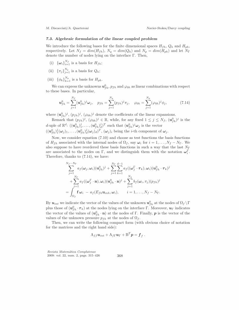
M. Discacciati/A. Quarteroni Navier-Stokes/Darcy coupling
7.3. Algebraic formulation of the linear coupled problem
We introduce the following bases for the finite dimensional spaces Hfh, Qh and Hph,respectively. Let Nf = dim(Hfh), Nq = dim(Qh) and Np = dim(Hph) and let NΓ
denote the number of nodes lying on the interface Γ. Then,
(i) ωiNf
i=1 is a basis for Hfh;
(ii) πjNq
j=1 is a basis for Qh;
(iii) φkNp
k=1 is a basis for Hph.
We can express the unknowns u0fh, pfh and ϕ0h as linear combinations with respect
to these bases. In particular,
u0fh =
Nf∑
j=1
(u0fh)jωj , pfh =
Nq∑
j=1
(pfh)jπj , ϕ0h =
Np∑
j=1
(ϕ0h)jφj , (7.14)
where (u0fh)j , (pfh)j , (ϕ0h)j denote the coefficients of the linear expansions.
Remark that (pfh)j , (ϕ0h)j ∈ R, while, for any fixed 1 ≤ j ≤ Nf , (u0fh)j is the
d-uple of Rd: ((u0
fh)j1, . . . , (u
0fh)j
d)T such that (u0
fh)jωj is the vector
((u0fh)j
1(ωj)1, . . . , (u0fh)j
d(ωj)d)T , (ωj)i being the i-th component of ωj .
Now, we consider equation (7.10) and choose as test functions the basis functionsof Hfh associated with the internal nodes of Ωf , say ωi for i = 1, . . . , Nf −NΓ. Wealso suppose to have reordered these basis functions in such a way that the last NΓ
are associated to the nodes on Γ, and we distinguish them with the notation ωΓi .
Therefore, thanks to (7.14), we have:
Nf−NΓ∑
j=1
af (ωj ,ωi)(u0fh)j +
NΓ∑
j=1
d−1∑
k=1
af ((ωΓj · τ k),ωi)(u
0fh · τ k)j
+
NΓ∑
j=1
af ((ωΓj · n),ωi)(u
0fh · n)j +
Nq∑
j=1
bf(ωi, πj)(pfh)j
=
∫
Ωf
f ωi − af (Efhuinh,ωi), i = 1, . . . , Nf −NΓ.
By uint we indicate the vector of the values of the unknown u0fh at the nodes of Ωf \Γ
plus those of (u0fh · τ k) at the nodes lying on the interface Γ. Moreover, uΓ indicates
the vector of the values of (u0fh · n) at the nodes of Γ. Finally, p is the vector of the
values of the unknown pressure pfh at the nodes of Ωf .Then, we can write the following compact form (with obvious choice of notation
for the matrices and the right hand side):
Affuint + AfΓuΓ + BT p = f f .
Revista Matematica Complutense
2009: vol. 22, num. 2, pags. 315–426 368
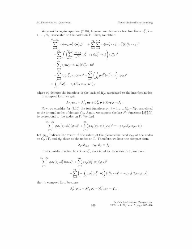
M. Discacciati/A. Quarteroni Navier-Stokes/Darcy coupling
We consider again equation (7.10), however we choose as test functions ωΓi , i =
1, . . . , NΓ, associated to the nodes on Γ. Then, we obtain:
Nf−NΓ∑
j=1
af (ωj ,ωΓi )(u0
fh)j +
NΓ∑
j=1
d−1∑
k=1
af ((ωΓj · τ k),ωΓ
i )(u0fh · τ k)j
+
NΓ∑
j=1
∫
Γ
(
d−1∑
k=1
ναBJ√K
(ωΓi · τ k)(ωΓ
j · τ k)
)
(u0fh)j
+
NΓ∑
j=1
af (ωΓj · n,ωΓ
i )(u0fh · n)j
+
Nq∑
j=1
bf(ωΓi , πj)(pfh)j +
NΓ∑
j=1
(∫
Γ
g φΓj (ωΓ
i · n)
)
(ϕ0h)j
=
∫
Ωf
f ωΓi − af (Efhuinh,ω
Γi ) ,
where φΓj denotes the functions of the basis of Hph associated to the interface nodes.
In compact form we get:
AΓfuint + AfΓΓuΓ + BT
fΓp + MΓΓφ = fΓ .
Now, we consider for (7.10) the test functions φi, i = 1, . . . , Np −NΓ, associated
to the internal nodes of domain Ωp. Again, we suppose the last NΓ functions φΓi NΓ
i=1
to correspond to the nodes on Γ. We find:
Np−NΓ∑
j=1
g ap(φj , φi) (ϕ0h)j +
NΓ∑
j=1
g ap(φΓj , φi) (ϕ0h)j = −g ap(Ephϕph, φi) .
Let φint indicate the vector of the values of the piezometric head ϕ0h at the nodeson Ωp \ Γ, and φΓ those at the nodes on Γ. Therefore, we have the compact form:
Appφint + ApΓφΓ = fp .
If we consider the test functions φΓi , associated to the nodes on Γ, we have:
Np−NΓ∑
j=1
g ap(φj , φΓi )(ϕ0h)j +
NΓ∑
j=1
g ap(φΓj , φ
Γi )(ϕ0h)j
+
NΓ∑
j=1
(
−∫
Γ
g φΓi (ωΓ
j · n)
)
(u0fh · n)j = −g ap(Ephϕph, φ
Γi ),
that in compact form becomes
ATpΓφint + Ap
ΓΓφΓ − MTΓΓuΓ = fpΓ .
369Revista Matematica Complutense
2009: vol. 22, num. 2, pags. 315–426
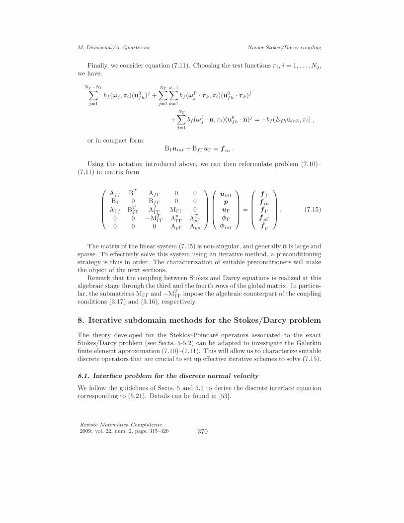
M. Discacciati/A. Quarteroni Navier-Stokes/Darcy coupling
Finally, we consider equation (7.11). Choosing the test functions πi, i = 1, . . . , Nq,we have:
Nf−NΓ∑
j=1
bf (ωj , πi)(u0fh)j +
NΓ∑
j=1
d−1∑
k=1
bf (ωΓj · τ k, πi)(u
0fh · τ k)j
+
NΓ∑
j=1
bf (ωΓj · n, πi)(u
0fh · n)j = −bf(Efhuinh, πi) ,
or in compact form:B1uint + BfΓuΓ = f in .
Using the notation introduced above, we can then reformulate problem (7.10)–(7.11) in matrix form
Aff BT AfΓ 0 0B1 0 BfΓ 0 0
AΓf BTfΓ Af
ΓΓ MΓΓ 0
0 0 −MTΓΓ Ap
ΓΓ ATpΓ
0 0 0 ApΓ App
uint
p
uΓ
φΓ
φint
=
f f
f in
fΓ
fpΓ
fp
. (7.15)
The matrix of the linear system (7.15) is non-singular, and generally it is large andsparse. To effectively solve this system using an iterative method, a preconditioningstrategy is thus in order. The characterization of suitable preconditioners will makethe object of the next sections.
Remark that the coupling between Stokes and Darcy equations is realized at thisalgebraic stage through the third and the fourth rows of the global matrix. In particu-lar, the submatrices MΓΓ and −MT
ΓΓ impose the algebraic counterpart of the couplingconditions (3.17) and (3.16), respectively.
8. Iterative subdomain methods for the Stokes/Darcy problem
The theory developed for the Steklov-Poincare operators associated to the exactStokes/Darcy problem (see Sects. 5-5.2) can be adapted to investigate the Galerkinfinite element approximation (7.10)–(7.11). This will allow us to characterize suitablediscrete operators that are crucial to set up effective iterative schemes to solve (7.15).
8.1. Interface problem for the discrete normal velocity
We follow the guidelines of Sects. 5 and 5.1 to derive the discrete interface equationcorresponding to (5.21). Details can be found in [53].
Revista Matematica Complutense
2009: vol. 22, num. 2, pags. 315–426 370
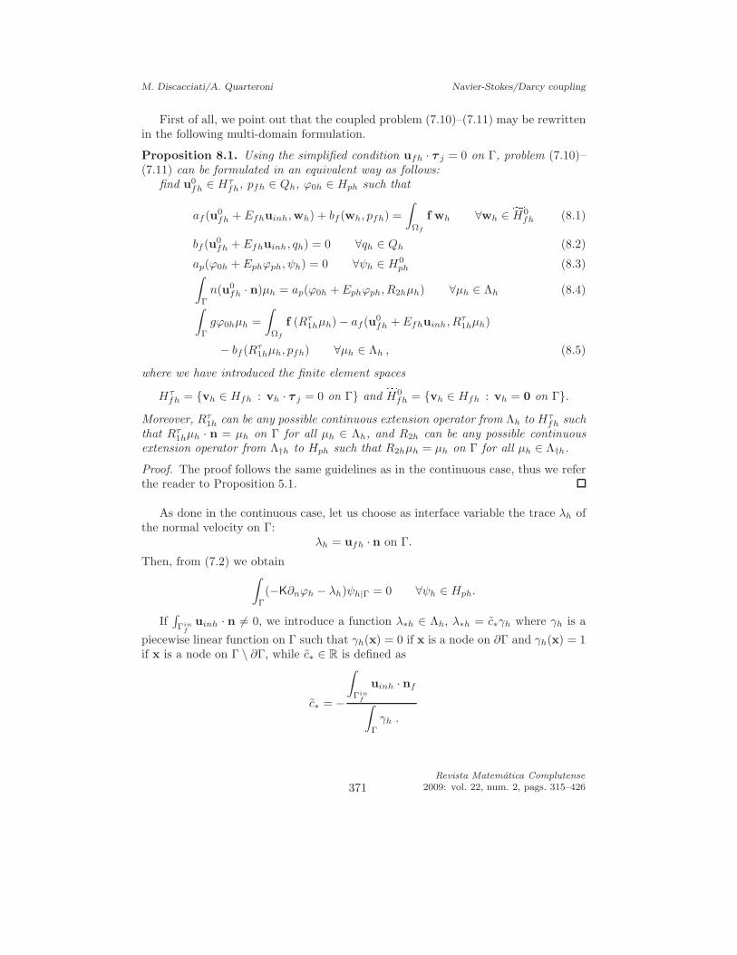
M. Discacciati/A. Quarteroni Navier-Stokes/Darcy coupling
First of all, we point out that the coupled problem (7.10)–(7.11) may be rewrittenin the following multi-domain formulation.
Proposition 8.1. Using the simplified condition ufh · τ j = 0 on Γ, problem (7.10)–(7.11) can be formulated in an equivalent way as follows:
find u0fh ∈ Hτ
fh, pfh ∈ Qh, ϕ0h ∈ Hph such that
af(u0fh + Efhuinh,wh) + bf(wh, pfh) =
∫
Ωf
f wh ∀wh ∈fH0fh (8.1)
bf(u0fh + Efhuinh, qh) = 0 ∀qh ∈ Qh (8.2)
ap(ϕ0h + Ephϕph, ψh) = 0 ∀ψh ∈ H0ph (8.3)
∫
Γ
n(u0fh · n)µh = ap(ϕ0h + Ephϕph, R2hµh) ∀µh ∈ Λh (8.4)
∫
Γ
gϕ0hµh =
∫
Ωf
f (Rτ1hµh) − af(u0
fh + Efhuinh, Rτ1hµh)
− bf(Rτ1hµh, pfh) ∀µh ∈ Λh , (8.5)
where we have introduced the finite element spaces
Hτfh = vh ∈ Hfh : vh · τ j = 0 on Γ and fH0
fh = vh ∈ Hfh : vh = 0 on Γ.Moreover, Rτ
1h can be any possible continuous extension operator from Λh to Hτfh such
that Rτ1hµh · n = µh on Γ for all µh ∈ Λh, and R2h can be any possible continuous
extension operator from Λ†h to Hph such that R2hµh = µh on Γ for all µh ∈ Λ†h.
Proof. The proof follows the same guidelines as in the continuous case, thus we referthe reader to Proposition 5.1.
As done in the continuous case, let us choose as interface variable the trace λh ofthe normal velocity on Γ:
λh = ufh · n on Γ.
Then, from (7.2) we obtain∫
Γ
(−K∂nϕh − λh)ψh|Γ = 0 ∀ψh ∈ Hph.
If∫
Γinf
uinh · n 6= 0, we introduce a function λ∗h ∈ Λh, λ∗h = c∗γh where γh is a
piecewise linear function on Γ such that γh(x) = 0 if x is a node on ∂Γ and γh(x) = 1if x is a node on Γ \ ∂Γ, while c∗ ∈ R is defined as
c∗ = −
∫
Γinf
uinh · nf
∫
Γ
γh .
371Revista Matematica Complutense
2009: vol. 22, num. 2, pags. 315–426
M. Discacciati/A. Quarteroni Navier-Stokes/Darcy coupling
Then∫
Γ
λ∗h = −∫
Γinf
uinh · nf . (8.6)
We introduce the space
Λ0h =
µh ∈ Λh :
∫
Γ
µh = 0
,
and we define the following extension operators:
Rfh : Λ0h → Hτfh ×Q0h, ηh → Rfhηh = (R1
fhηh, R2fhηh),
such that (R1fhηh) · n = ηh on Γ and
af (R1fhηh,wh) + bf (wh, R
2fhηh) = 0 ∀wh ∈ H0
fh,
bf (R1fhηh, qh) = 0 ∀qh ∈ Q0h,
andRph : Λ0h → Hph, ηh → Rphηh,
such that
ap(Rphηh, R2hµh) =
∫
Γ
nηhµh ∀µh ∈ Λ†h, (8.7)
where R2h is the extension operator introduced in Proposition 8.1.
Now we can define the discrete Steklov-Poincare operator Sh : Λ0h → Λ′h, for all
ηh ∈ Λ0h and for all µh ∈ Λh, as follows:
〈Shηh, µh〉 = af (R1fhηh, R
τ1hµh) + bf(Rτ
1hµh, R2fhηh) +
∫
Γ
g(Rphηh)µh.
Sh can be split as sum of two suboperators Sh = Sfh+Sph, associated with the Stokesand Darcy problems, respectively, and defined respectively by
〈Sfhηh, µh〉 = af (R1fhηh, R
τ1hµh) + bf (Rτ
1hµh, R2fhηh) , (8.8)
〈Sphηh, µh〉 =
∫
Γ
g (Rphηh)µh ,
for all ηh ∈ Λ0h, µh ∈ Λh.Finally, let χh be the linear functional which represents the Galerkin counterpart
of (5.19).
A reinterpretation of problem (8.1)–(8.5) in terms of a Steklov-Poincare discreteinterface problem is provided by the following result, which is the discrete counterpartof Theorem 5.3.
Revista Matematica Complutense
2009: vol. 22, num. 2, pags. 315–426 372
M. Discacciati/A. Quarteroni Navier-Stokes/Darcy coupling
Theorem 8.2. The solution to (8.1)–(8.5) can be characterized as follows:
u0fh = ω∗
0h +R1fhλ0h + EΓhλ∗h, pfh = π∗
h +R2fhλ0h + pfh,
ϕ0h = ϕ∗0h +Rphλ0h ,
where pfh = (meas(Ωf ))−1∫
Ωfph, and λ0h ∈ Λ0h is the solution of the discrete
Steklov-Poincare interface problem:
〈Shλ0h, µ0h〉 = 〈χh, µ0h〉 ∀µ0h ∈ Λ0h . (8.9)
Moreover, pfh can be obtained from λ0h by solving the algebraic equation
pfh =1
meas(Γ)〈Shλ0h − χh, ζh〉 ,
where ζh ∈ Λh is a given function that satisfies
1
meas(Γ)
∫
Γ
ζh = 1 .
8.2. Analysis of the discrete Steklov-Poincare operators Sfh and Sph
Let us investigate some properties of the discrete Steklov-Poincare operators Sfh, Sph
and Sh that will allow us to prove existence and uniqueness for problem (8.9). Sincetheir proof is similar to the one of the continuous case, we shall only sketch them,referring to Lemma 5.4 for more details.
Lemma 8.3. The discrete Steklov–Poincare operators enjoy the following properties:
(i) Sfh and Sph are linear continuous operators on Λ0h, i.e., Sfhηh ∈ Λ′0, Sphηh ∈
Λ′0, ∀ηh ∈ Λ0h ;
(ii) Sfh is symmetric and coercive;
(iii) Sph is symmetric and positive;
(iv) Sh and Sfh are uniformly spectrally equivalent, i.e., there exist two constants
k1 and k2 independent of h, such that ∀ηh ∈ Λh,
k1〈Sfhηh, ηh〉 ≤ 〈Shηh, ηh〉 ≤ k2〈Sfhηh, ηh〉.
Proof. 1. Making the special choice Rτ1h = R1
fh, the operator Sfh can be representedas follows
〈Sfhηh, µh〉 = af (R1fhηh, R
1fhµh) ∀ηh, µh ∈ Λ0h. (8.10)
Now, proceeding as done at point 1. of Lemma 5.4, we can define the functionzh(µh) = R1
fhµh−Hhµh ∈fH0fh, Hh being the Galerkin approximation of the harmonic
extension operator defined in (5.25).
373Revista Matematica Complutense
2009: vol. 22, num. 2, pags. 315–426
M. Discacciati/A. Quarteroni Navier-Stokes/Darcy coupling
Using the inf-sup condition (5.3.43) of [109, page 173], we have for all µh ∈ Λ0h
‖R2fhµh‖0 ≤ ν
β∗‖R1
fhµh‖1 ,
and therefore
‖R1fhµh‖1 ≤ (1 + CΩf
)
(
1 +1
β∗
)
‖Hhµh‖1 , (8.11)
CΩfbeing a positive constant due to the Poincare inequality. Now, thanks to the
Uniform Extension Theorem (see [109, Theorem 4.1.3] and [94]), there exists a positiveconstant C|Ωf | > 0, depending on the measure of the subdomain Ωf , but independentof the parameter h, such that
‖Hhµh‖1 ≤ C|Ωf |‖µh‖Λ ∀µh ∈ Λh.
Therefore, (8.11) yields ∀µh ∈ Λ0h
‖R1fhµh‖1 ≤ C|Ωf |(1 + CΩf
)
(
1 +1
β∗
)
‖µh‖Λ . (8.12)
From (8.12) we deduce the continuity of Sfh:
|〈Sfhµh, ηh〉| ≤ βf‖µh‖Λ‖ηh‖Λ ,
where βf is the following positive constant, independent of h,
βf = ν
[
C|Ωf |(1 + CΩf)
(
1 +1
β∗
)]2
. (8.13)
Proceeding as for the continuous case, we can prove that Sph is continuous withconstant βp, independent of h, defined in (5.31).
2. Sfh is symmetric thanks to (8.10) and the proof of its coercivity follows the one inthe continuous case, the coercivity constant αf being the same (see (5.32)).
3. This property follows from point 3. of the proof of Lemma 5.4.
Remark 8.4. Notice that the discrete operator Sph is actually coercive (see, e.g.,[45, 7]); however, its coercivity constant, say αph > 0 depends on h and, in particular,it vanishes as h → 0. Since we are primarily looking for preconditioners for theinterface problem (8.9) which are optimal with respect to h, we will not consider Sph
as a possible preconditioner any longer.
Remark 8.5. Thanks to Lax-Milgram Lemma (see, e.g., [109, page 133]), Lemma 8.3guarantees that the discrete Steklov-Poincare equation (8.9) has a unique solution.
Revista Matematica Complutense
2009: vol. 22, num. 2, pags. 315–426 374

M. Discacciati/A. Quarteroni Navier-Stokes/Darcy coupling
8.3. Algebraic formulation of the discrete Steklov-Poincare operator Sh
We consider the linear system (7.15) and we set uf = (uint,p)T and φ = (φΓ,φint)T .
Then, with obvious choice of notation, we can rewrite (7.15) in the following blockform:
F F1Γ 0
F2Γ Af
ΓΓ M1
0 M2 D
uf
uΓ
φ
=
f1
fΓ
f2
. (8.14)
By writing uΓ = u0Γ + λ∗, where λ∗ is the vector whose components are the
(known) values of λ∗h at the nodes on Γ, system (8.14) reduces to:
F F1Γ 0
F2Γ Af
ΓΓ M1
0 M2 D
uf
u0Γ
φ
=
f1
fΓ
f2
where f1 = f1 − F1Γλ∗, fΓ = fΓ − Af
ΓΓλ∗ and f2 = f2 − M2λ∗.
Upon eliminating the unknowns uf and φ, we obtain the reduced Schur comple-ment system:
Σhu0Γ = χh, (8.15)
where we have defined
Σh = AfΓΓ − F2
ΓF−1F1Γ − M1D
−1M2 (8.16)
and
χh = fΓ − F2ΓF−1f1 − M1D
−1f2 .
In (8.16) the first term
Σfh = AfΓΓ − F2
ΓF−1F1Γ (8.17)
arises from domain Ωf , whereas
Σph = −M1D−1M2 (8.18)
from Ωp. The matrices Σfh and Σph are the algebraic counterparts of the operatorsSfh and Sph, respectively.
Remark 8.6. To be precise, notice that we are slightly abusing in notation, sincefor the algebraic system (7.15) we have considered the complete interface condition(3.18), while in order to characterize the discrete Steklov-Poincare operators we haveused its simplified form ufh · τ j = 0 on Γ. Therefore, the exact algebraic counterpartof Sfh and Sph should be obtained considering a basis of Hτ
fh rather than Hfh.
375Revista Matematica Complutense
2009: vol. 22, num. 2, pags. 315–426
M. Discacciati/A. Quarteroni Navier-Stokes/Darcy coupling
Thanks to Lemma 8.3, the matrices Σfh and Σh are symmetric and positive defi-nite. Moreover
[Σfhµ,µ] ≤ [Σhµ,µ] ≤(
1 +βp
αf
)
[Σfhµ,µ] ∀µ ∈ RNΓ ,
where [., .] is the Euclidean scalar product in RNΓ and αf and βp are the constants
defined in (5.32) and (5.31), respectively.
Thus, the spectral condition number χsp of the matrix Σ−1fhΣh is bounded inde-
pendently of h:
χsp(Σ−1fhΣh) ≤ 1 +
βp
αf,
and Σfh is an optimal preconditioner for Σh. Therefore, should we use Σfh as precon-ditioner to solve the symmetric linear system (8.15) using the preconditioned Richard-son method
(u0Γ)k+1 = (u0
Γ)k + Σ−1fh (χh − Σh(u0
Γ)k), (8.19)
we would get convergence with a rate independent of h. Same conclusion if insteadof (8.19) we would use a Krylov type method (e.g., the conjugate gradient method).
In the next section, we shall interpret (8.19) as a Dirichlet-Neumann substructur-ing scheme and we shall prove its convergence.
8.4. A subdomain iterative method for the Stokes/Darcy problem
The iterative method we propose to compute the solution of the Stokes/Darcy problem(8.1)–(8.5) consists in solving first Darcy problem in Ωp imposing the continuity ofthe normal velocities across Γ. Then, we solve the Stokes problem in Ωf imposing thecontinuity of the normal stresses across the interface, using the value of ϕh on Γ thatwe have just computed in the porous media domain. Precisely, the iterative schemereads as follows.
Given uinh, construct λ∗h as in (8.6). Then, let λ0h ∈ Λ0h be the initial guess, and,
for k ≥ 0:
(i) Find ϕk+10h ∈ Hph such that, for all ψh ∈ Hph,
ap(ϕk+10h , ψh) −
∫
Γ
nψh λk0h = −ap(Ephϕph, ψh) +
∫
Γ
nψhλ∗h. (8.20)
Revista Matematica Complutense
2009: vol. 22, num. 2, pags. 315–426 376
M. Discacciati/A. Quarteroni Navier-Stokes/Darcy coupling
(ii) Find (u0fh)k+1 ∈ Hτ
fh, pk+1fh ∈ Qh:
af ((u0fh)k+1,wh) + bf(wh, p
k+1fh ) +
∫
Γ
gϕk+1h wh · n
=
∫
Ωf
f wh − af (Efhuinh,wh) ∀wh ∈ Hτfh, (8.21)
bf ((u0fh)k+1, qh) = −bf(Efhuinh, qh) ∀qh ∈ Qh, (8.22)
with ϕk+1h = ϕk+1
0h + Ephϕph.
(iii) Update λk0h:
λk+10h = θ(uk+1
fh · n− λ∗h)|Γ + (1 − θ)λk0h , (8.23)
θ being a positive relaxation parameter and uk+1fh = (u0
fh)k+1 + Efhuinh.
Remark 8.7. Note that λk0h ∈ Λ0h for all k ≥ 0. In fact, λ0h ∈ Λ0h given, suppose
λk0h ∈ Λ0. Then
∫
Γ
λk+10h = θ
∫
Γ
(uk+1fh · n|Γ − λ∗h) .
Now, since∫
Ωf∇ · uk+1
fh = 0, thanks to the divergence theorem we have
∫
Γ
uk+1fh · n = −
∫
Γinf
uinh · n
and recalling (8.6) the thesis follows.
Following the general theory developed in [110], the above iterative method canbe reinterpreted as a preconditioned Richardson method for the Steklov–Poincareproblem (8.9).
Lemma 8.8. The iterative substructuring scheme (8.20)–(8.23) to compute the solu-tion of the finite element approximation of the coupled problem Stokes/Darcy (8.1)–(8.5) is equivalent to a preconditioned Richardson method for the discrete Steklov-Poincare equation (8.9), the preconditioner being the operator Sfh introduced in (8.8).
Proof. Since Efhuinh · n = 0 on Γ, (8.23) reduces to:
λk+10h = θ((u0
fh)k+1 · n − λ∗h)|Γ + (1 − θ)λk0h .
Let Rτ1h : Λh → Hτ
fh be the extension operator introduced in Proposition 8.1. For allµh ∈ Λh, we can rewrite (8.21) as:
af ((u0fh)k+1, Rτ
1hµh) + bf (Rτ1hµh, p
k+1fh ) +
∫
Γ
gϕk+1h µh
=
∫
Ωf
f (Rτ1hµh) − af (Efhuinh, R
τ1hµh) ∀µh ∈ Λh. (8.24)
377Revista Matematica Complutense
2009: vol. 22, num. 2, pags. 315–426
M. Discacciati/A. Quarteroni Navier-Stokes/Darcy coupling
Let us define pk+1fh = (meas(Ωf ))−1
∫
Ωfpk+1
fh ; then we set
pk+10h = pk+1
fh − pk+1fh ,
and we note that pk+10h ∈ Q0. Then (8.24) gives:
af ((u0fh)k+1, Rτ
1hµh) + bf (Rτ1hµh, p
k+10h ) +
∫
Γ
gϕk+1h µh
=
∫
Ωf
f (Rτ1hµh) + bf (Rτ
1hµh, pk+1fh ) − af (Efhuinh, R
τ1hµh) ∀µh ∈ Λh. (8.25)
Let ω∗0h, π∗
h be the solution to the following problem:
find ω∗0h ∈fH0
fh, π∗h ∈ Q0h such that for all vh ∈fH0
fh, qh ∈ Q0h
af (ω∗0h + Efhuinh + EΓhλ∗h,vh) + bf (vh, π
∗h) =
∫
Ωf
f vh,
bf(ω∗0h + Efhuinh + EΓhλ∗h, qh) = 0 ,
where we have set Q0h = qh ∈ Qh :∫
Ωfqh = 0 and EΓhλ∗h ∈ Hτ
fh denotes a
suitable discrete extension of λ∗h, such that EΓhλ∗h · n = λ∗h on Γ. Moreover, letϕ∗
0h ∈ Hph be such that
ap(ϕ∗0h + Ephϕph, ψh) =
∫
Γ
nλ∗hψh ∀ψh ∈ Hph. (8.26)
Subtracting from both members in (8.25) the following terms:
af (ω∗0h + EΓhλh∗, R
τ1hµh) + bf (Rτ
1hµh, π∗h) +
∫
Γ
g ϕ∗0hµh ,
we have, for all µh ∈ Λh,
af ((u0fh)k+1 − ω∗
0h − EΓhλh∗, Rτ1hµh) + bf (Rτ
1hµh, pk+10h − π∗
h)
+
∫
Γ
g(ϕk+1h − ϕ∗
0h)µh
=
∫
Ωf
f (Rτ1hµh) − bf (Rτ
1hµh, π∗h)
− af (ω∗0h + EΓhλh∗
+ Efhuinh, Rτ1hµh) −
∫
Γ
g ϕ∗0hµh + bf (Rτ
1hµh, pk+1fh ). (8.27)
Since∫
Ωf
∇ · (ω∗0 + EΓhλ∗h + Efhuinh) = 0
Revista Matematica Complutense
2009: vol. 22, num. 2, pags. 315–426 378
M. Discacciati/A. Quarteroni Navier-Stokes/Darcy coupling
and∫
Ωf
∇ · ((u0fh)k+1 + Efhuinh) = 0,
we obtain∫
Ω
∇ · ((u0fh)k+1 − ω∗
0 − EΓhλ∗h) = 0.
Now, if we apply the divergence theorem and recall that (u0fh)k+1 ∈ Hτ
fh, ω∗0h ∈fH0
fh
and EΓhλ∗h ∈ Hτfh, we see that [(u0
fh)k+1 −EΓhλ∗h] ·n|Γ ∈ Λ0h. Therefore, using thedefinition (8.8) of Sfh, we have:
af ((u0fh)k+1 − ω∗
0h − EΓhλ∗h, Rτ1hµh) + bf (Rτ
1hµh, pk+10h − π∗
h)
= 〈Sfh(((u0fh)k+1 − EΓhλ∗h) · n)|Γ, µh〉
for all µh ∈ Λh.Moreover, if we subtract (8.26) from (8.20), we obtain
ap(ϕk+10h − ϕ∗
0h, ψh) =
∫
Γ
nλk0hψh ∀ψh ∈ Hph ,
whence, thanks to (8.7), ϕk+10h − ϕ∗
0h = Rphλk0h. Therefore
∫
Γ
g(ϕk+1h − ϕ∗
0h)µh = 〈Sphλk0h, µh〉 ∀µh ∈ Λh.
Finally, if we apply the divergence theorem to the last term on the right hand side of(8.27) and we use the definition of χh, we can rewrite the right hand side of (8.27) as
〈χh, µh〉 + pk+1fh
∫
Γ
µh ∀µh ∈ Λh .
Now, for all µh ∈ Λ0h, it follows:
〈Sfh(((u0fh)k+1 − EΓhλ∗h) · n)|Γ, µh〉 + 〈Sphλ
k0h, µh〉 = 〈χh, µh〉 .
Therefore we can conclude that (8.20)–(8.23) is equivalent to the preconditioned Ri-chardson scheme: let λ0
0h ∈ Λ0h be given; for k ≥ 0, find λk+10h ∈ Λ0h s.t.
λk+10h = λk
0h + θhS−1fh (χh − Shλ
k0h) . (8.28)
Remark 8.9. The algorithm (8.20)–(8.23) does not feature the classical structure of aDirichlet-Neumann method, which would require to solve one subproblem in the firstsubdomain with a Dirichlet boundary condition on the interface, and one problem
379Revista Matematica Complutense
2009: vol. 22, num. 2, pags. 315–426
M. Discacciati/A. Quarteroni Navier-Stokes/Darcy coupling
in the second subdomain with a Neumann boundary condition on the interface. Asa matter of fact, the condition that we are imposing for the first subdomain Ωp isa Neumann (rather than a Dirichlet) natural condition on Γ. However, in view of(8.28), it shares with the Dirichlet-Neumann method the fact that the preconditionerof the Richardson iterations is the Steklov-Poincare operator associated to the secondsubdomain Ωp.
The formulation (8.28) is very convenient for the analysis of convergence of theiterative scheme (8.20)–(8.23). Indeed, with this aim we can apply the followingabstract convergence result (see [110, Theorem 4.2.2 and Remark 4.2.4]).
Lemma 8.10. Let X be a (real) Hilbert space and X ′ be its dual. We consider alinear invertible continuous operator Q : X → X ′, which can be split as Q = Q1 +Q2,where both Q1 and Q2 are linear operators. Taken Z ∈ X ′, let x ∈ X be the unknownsolution to the equation
Qx = Z , (8.29)
and consider for its solution the preconditioned Richardson method
Q2(xk+1 − xk) = θ(Z −Qxk), k ≥ 0,
θ being a positive relaxation parameter. Suppose that the following conditions aresatisfied:
(i) Q2 is symmetric, continuous with constant β2 and coercive with constant α2;
(ii) Q1 is continuous with constant β1;
(iii) Q is coercive with constant αQ.
Then, for any given x0 ∈ X and for any 0 < θ < θmax, with
θmax =2αQα
22
β2(β1 + β2)2,
the sequence
xk+1 = xk + θQ−12 (Z −Qxk)
converges in X to the solution of problem (8.29).
We can now prove the main result of this section.
Theorem 8.11. For any choice of the initial guess λ00h ∈ Λ0h and for suitable val-
ues of the relaxation parameter θ the iterative method (8.20)–(8.23) converges to thesolution (u0
fh, pfh, ϕ0h) ∈ Hτfh×Qh×Hph of the coupled Stokes/Darcy problem (8.1)–
(8.5).
Revista Matematica Complutense
2009: vol. 22, num. 2, pags. 315–426 380
M. Discacciati/A. Quarteroni Navier-Stokes/Darcy coupling
Proof. Upon setting X = Λ0h, Q = Sh, Q1 = Sph, Q2 = Sfh and Z = χh, the prooffollows from Theorem 8.10, whose hypotheses are satisfied thanks to Lemma 8.3. Infact, for any initial guess λ0
0h ∈ Λ0h, and any 0 < θ < θmax with
θmax =2α3
f
βf (βf + βp)2,
the sequence defined in (8.28) converges to the solution of the Steklov–Poincare equa-tion (8.9). Taking the limit k → ∞ in the iterative procedure (8.20)–(8.23), it followsthat ((u0
fh)k, pkfh, ϕ
k0h)k → (u0
fh, pfh, ϕ0h).
The upper bound θmax is independent of h as such are the constants αf , βf
and βp. (We recall that the constants αf , βf and βp are respectively the coercivityand the continuity constants of the operator Sfh and the continuity constant of Sph,and they have been introduced in (5.32), (8.13) and (5.31), respectively. See alsoLemma 8.3.)
8.5. Matrix interpretation of the subdomain iterative method
The iterative scheme (8.20)–(8.23) corresponds to the following steps.Let λk
0 ∈ RNΓ be the vector of the values of λk
0h at the k-th step at the nodes of Γ.Problem (8.20) yields the following algebraic system:
(
ApΓΓ AT
pΓ
ApΓ App
)(
φk+1Γ
φk+1int
)
=
(
fpΓ + MTΓλk
0 + MTΓλ∗
fp
)
, (8.30)
where φk+1Γ and φk+1
int are the vectors of the nodal values of the solution ϕk+10h at the
interface and internal nodes, respectively.By formally eliminating φk+1
int from (8.30), we obtain
(ApΓΓ −AT
pΓA−1pp ApΓ)φk+1
Γ = fpΓ − ATpΓA−1
pp fp + MTΓλk + MT
Γλ∗.
Now use φk+1Γ to compute the unknown vector uk+1
Γ by solving the followingsystem, which corresponds to the Stokes problem (8.21)–(8.22):
Aff BT AfΓ
B1 0 BfΓ
AfΓ BTfΓ Af
ΓΓ
uk+1int
pk+1
uk+1Γ
=
f f
f in
fΓ − MΓφk+1Γ
.
The vectors uk+1int and pk+1 contain respectively the nodal values of (u0
fh)k+1 and of
the pressure pk+1fh at the internal points of Ωf , while uk+1
Γ the nodal values of the
normal velocity uk+1fh · n on Γ.
Finally, according to (8.23), we set
λk+10 = θ(uk+1
Γ − λ∗) + (1 − θ)λk0 ,
381Revista Matematica Complutense
2009: vol. 22, num. 2, pags. 315–426
M. Discacciati/A. Quarteroni Navier-Stokes/Darcy coupling
and we iterate restarting from (8.30) until the convergence test
‖λk+10 − λk
0‖RNΓ
‖λk+10 ‖
RNΓ
≤ ǫ
is satisfied for a prescribed tolerance ǫ; ‖ · ‖R
NΓ denotes the Euclidean norm in RNΓ .
9. Some numerical results for the Stokes/Darcy coupling
For the sake of clarity, before presenting the numerical results, we give a schematicoverview of the numerical algorithm we shall adopt, and we discuss the implementa-tion of the preconditioned conjugate gradient (PCG) methods (see, e.g., [114]) whichexploit the preconditioners Σfh of Section 8.3.
The method introduced in Sects. 8.4 and 8.5 can be written in the followingpseudo-algorithmic form.
Algorithm 1. Choose an initial guess (uf )0 · n on Γ. Then, for k = 0, 1, . . . untilconvergence, do
1. Solve Darcy equation with boundary condition −K∂nϕk+1 = uk
f · n on Γ.
2. Solve Stokes problem imposing −n · T(uk+ 1
2
f , pk+ 1
2
f ) · n = gϕk+1 on Γ.
3. Update: uk+1f · n = θ u
k+ 1
2
f · n + (1 − θ)ukf · n on Γ, with θ ∈ (0, 1).
On the other hand, the preconditioner Σfh can be used in the framework of PCGiterations to solve the symmetric positive definite Schur complement system (8.15).In this case, the algorithm reads as follows.
Algorithm 2. Given an initial guess (u0Γ)0 for the fluid velocity on Γ, set r0 =
χh − Σh(u0Γ)0, and w0 = z0 = Σ−1
fhr0. Then, for k ≥ 0:
vk = Σhwk, (9.1)
αk =[wk, rk]
[wk,vk],
(u0Γ)k+1 = (u0
Γ)k + αkwk,
rk+1 = rk − αkvk,
solve Σfhzk+1 = rk+1, (9.2)
βk =[vk, zk+1]
[wk,vk],
wk+1 = zk+1 − βkwk,
where [·, ·] denotes the Euclidean scalar product in RNΓ.
Revista Matematica Complutense
2009: vol. 22, num. 2, pags. 315–426 382
M. Discacciati/A. Quarteroni Navier-Stokes/Darcy coupling
The most expensive steps in terms of computational effort are (9.1) and (9.2).Indeed, step (9.1) requires
• to compute Σfhwk which amounts to solving a Stokes problem in Ωf with aDirichlet boundary condition on Γ (see the corresponding differential operatorSf in Section 5.2);
• to compute Σphwk which amounts to solve a Darcy problem in Ωp with Neu-mann boundary condition on Γ (see the definition of the corresponding differ-ential operator Sp in Section 5.2).
Step (9.2) demands to solve the linear system Σfhzk+1 = rk+1 ⇔ zk+1 =Σ−1
fhrk+1 which amounts to solve a Stokes problem in Ωf with Neumann boundary
condition on Γ (see also the definition of the differential operator S−1f in Section 5.2).
Each step of the PCG method requires therefore to solve one Darcy problem inΩp and two Stokes problems in Ωf .
9.1. Numerical tests with respect to the grid parameter
We investigate the convergence properties of Algorithms 1 and 2 with respect tothe grid parameter h. For the moment we set the physical parameters ν, K, g to1. We consider the computational domain Ω ⊂ R
2 with Ωf = (0, 1) × (1, 2), Ωp =(0, 1) × (0, 1) and the interface Γ = (0, 1) × 1. We impose Dirichlet boundaryconditions on the velocity on ∂Ωf \Γ, while we consider a Dirichlet boundary conditionϕ = ϕp on the bottom boundary (0, 1) × 0 and Neumann boundary conditions onthe lateral boundaries 0, 1× (0, 1) of the domain Ωp. The boundary conditions andthe forcing terms are chosen in such a way that the exact solution of the coupledStokes/Darcy problem is
(uf )1 = − cos(π
2y)
sin(π
2x)
, (uf )2 = sin(π
2y)
cos(π
2x)
− 1 + x,
pf = 1 − x, ϕ =2
πcos(π
2x)
cos(π
2y)
− y(x− 1),
where (uf )1 and (uf )2 are the components of the velocity field uf . Note in particularthat uf · τ = (uf )1 = 0 on Γ according to (5.7). Finally, remark that in Darcyequation a non null forcing term has been considered. This implies the presence of anadditional term in the definition of the functional F in (4.10), but it does not affectthe theory we have developed.
In our computation, four different regular conforming meshes have been consideredwhose number of elements in Ω and of nodes on Γ are reported in Table 2, togetherwith the number of iterations to convergence obtained using Algorithms 1 and 2.The P2 − P1 Taylor-Hood finite elements have been used for Stokes problem and P2
elements for Darcy equation.
383Revista Matematica Complutense
2009: vol. 22, num. 2, pags. 315–426
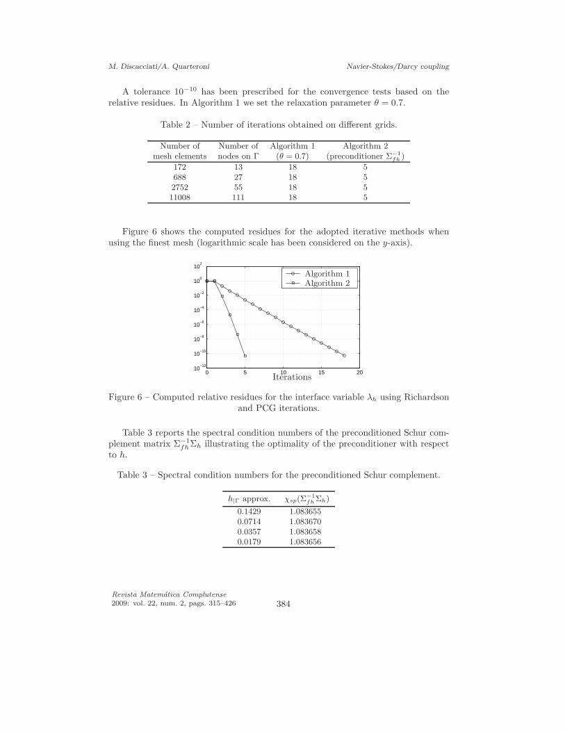
M. Discacciati/A. Quarteroni Navier-Stokes/Darcy coupling
A tolerance 10−10 has been prescribed for the convergence tests based on therelative residues. In Algorithm 1 we set the relaxation parameter θ = 0.7.
Table 2 – Number of iterations obtained on different grids.
Number of Number of Algorithm 1 Algorithm 2mesh elements nodes on Γ (θ = 0.7) (preconditioner Σ−1
fh )
172 13 18 5688 27 18 52752 55 18 511008 111 18 5
Figure 6 shows the computed residues for the adopted iterative methods whenusing the finest mesh (logarithmic scale has been considered on the y-axis).
0 5 10 15 2010
−12
10−10
10−8
10−6
10−4
10−2
100
102
Iterations
Algorithm 1Algorithm 2
Figure 6 – Computed relative residues for the interface variable λh using Richardsonand PCG iterations.
Table 3 reports the spectral condition numbers of the preconditioned Schur com-plement matrix Σ−1
fhΣh illustrating the optimality of the preconditioner with respectto h.
Table 3 – Spectral condition numbers for the preconditioned Schur complement.
h|Γ approx. χsp(Σ−1
fh Σh)
0.1429 1.0836550.0714 1.0836700.0357 1.0836580.0179 1.083656
Revista Matematica Complutense
2009: vol. 22, num. 2, pags. 315–426 384
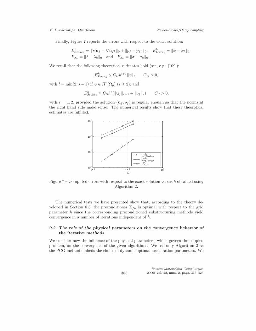
M. Discacciati/A. Quarteroni Navier-Stokes/Darcy coupling
Finally, Figure 7 reports the errors with respect to the exact solution:
EhStokes = ‖∇uf −∇ufh‖0 + ‖pf − pfh‖0, Eh
Darcy = ‖ϕ− ϕh‖1
Eλh= ‖λ− λh‖0 and Eσh
= ‖σ − σh‖0.
We recall that the following theoretical estimates hold (see, e.g., [109]):
EhDarcy ≤ CDh
l+1‖ϕ‖l CD > 0,
with l = min(2, s− 1) if ϕ ∈ Hs(Ωp) (s ≥ 2), and
EhStokes ≤ CSh
r(‖uf‖r+1 + ‖pf‖r) CS > 0,
with r = 1, 2, provided the solution (uf , pf ) is regular enough so that the norms atthe right hand side make sense. The numerical results show that these theoreticalestimates are fulfilled.
10−2
10−1
100
10−8
10−6
10−4
10−2
h
EhStokes
EhDarcy
Eλh
Figure 7 – Computed errors with respect to the exact solution versus h obtained usingAlgorithm 2.
The numerical tests we have presented show that, according to the theory de-veloped in Section 8.3, the preconditioner Σfh is optimal with respect to the gridparameter h since the corresponding preconditioned substructuring methods yieldconvergence in a number of iterations independent of h.
9.2. The role of the physical parameters on the convergence behavior ofthe iterative methods
We consider now the influence of the physical parameters, which govern the coupledproblem, on the convergence of the given algorithms. We use only Algorithm 2 asthe PCG method embeds the choice of dynamic optimal acceleration parameters. We
385Revista Matematica Complutense
2009: vol. 22, num. 2, pags. 315–426
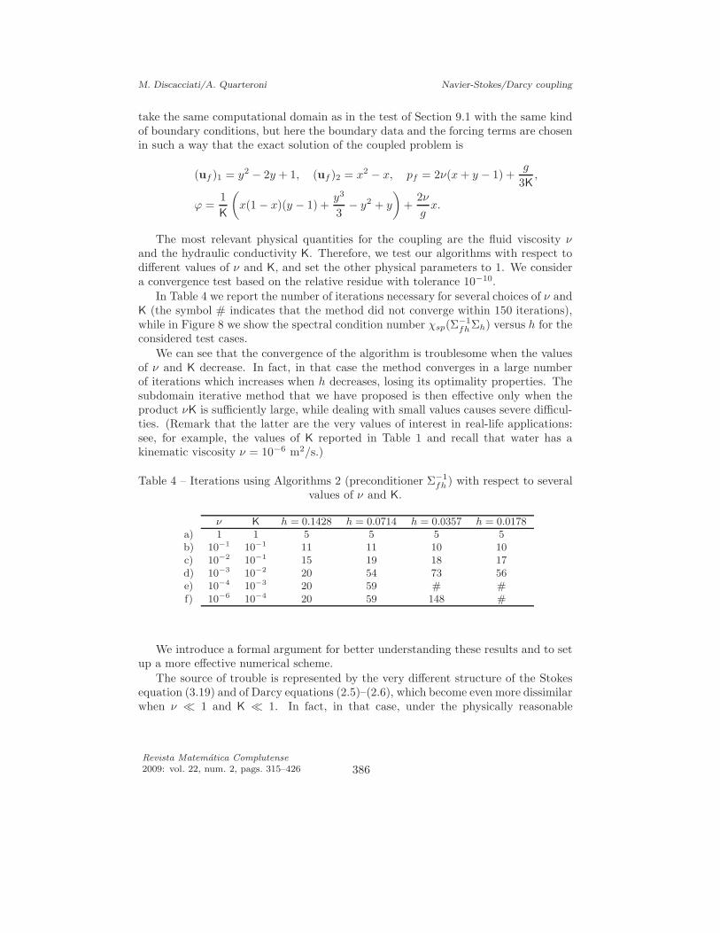
M. Discacciati/A. Quarteroni Navier-Stokes/Darcy coupling
take the same computational domain as in the test of Section 9.1 with the same kindof boundary conditions, but here the boundary data and the forcing terms are chosenin such a way that the exact solution of the coupled problem is
(uf )1 = y2 − 2y + 1, (uf )2 = x2 − x, pf = 2ν(x+ y − 1) +g
3K,
ϕ =1
K
(
x(1 − x)(y − 1) +y3
3− y2 + y
)
+2ν
gx.
The most relevant physical quantities for the coupling are the fluid viscosity νand the hydraulic conductivity K. Therefore, we test our algorithms with respect todifferent values of ν and K, and set the other physical parameters to 1. We considera convergence test based on the relative residue with tolerance 10−10.
In Table 4 we report the number of iterations necessary for several choices of ν andK (the symbol # indicates that the method did not converge within 150 iterations),while in Figure 8 we show the spectral condition number χsp(Σ
−1fhΣh) versus h for the
considered test cases.
We can see that the convergence of the algorithm is troublesome when the valuesof ν and K decrease. In fact, in that case the method converges in a large numberof iterations which increases when h decreases, losing its optimality properties. Thesubdomain iterative method that we have proposed is then effective only when theproduct νK is sufficiently large, while dealing with small values causes severe difficul-ties. (Remark that the latter are the very values of interest in real-life applications:see, for example, the values of K reported in Table 1 and recall that water has akinematic viscosity ν = 10−6 m2/s.)
Table 4 – Iterations using Algorithms 2 (preconditioner Σ−1fh ) with respect to several
values of ν and K.
ν K h = 0.1428 h = 0.0714 h = 0.0357 h = 0.0178a) 1 1 5 5 5 5b) 10−1 10−1 11 11 10 10c) 10−2 10−1 15 19 18 17d) 10−3 10−2 20 54 73 56e) 10−4 10−3 20 59 # #f) 10−6 10−4 20 59 148 #
We introduce a formal argument for better understanding these results and to setup a more effective numerical scheme.
The source of trouble is represented by the very different structure of the Stokesequation (3.19) and of Darcy equations (2.5)–(2.6), which become even more dissimilarwhen ν ≪ 1 and K ≪ 1. In fact, in that case, under the physically reasonable
Revista Matematica Complutense
2009: vol. 22, num. 2, pags. 315–426 386
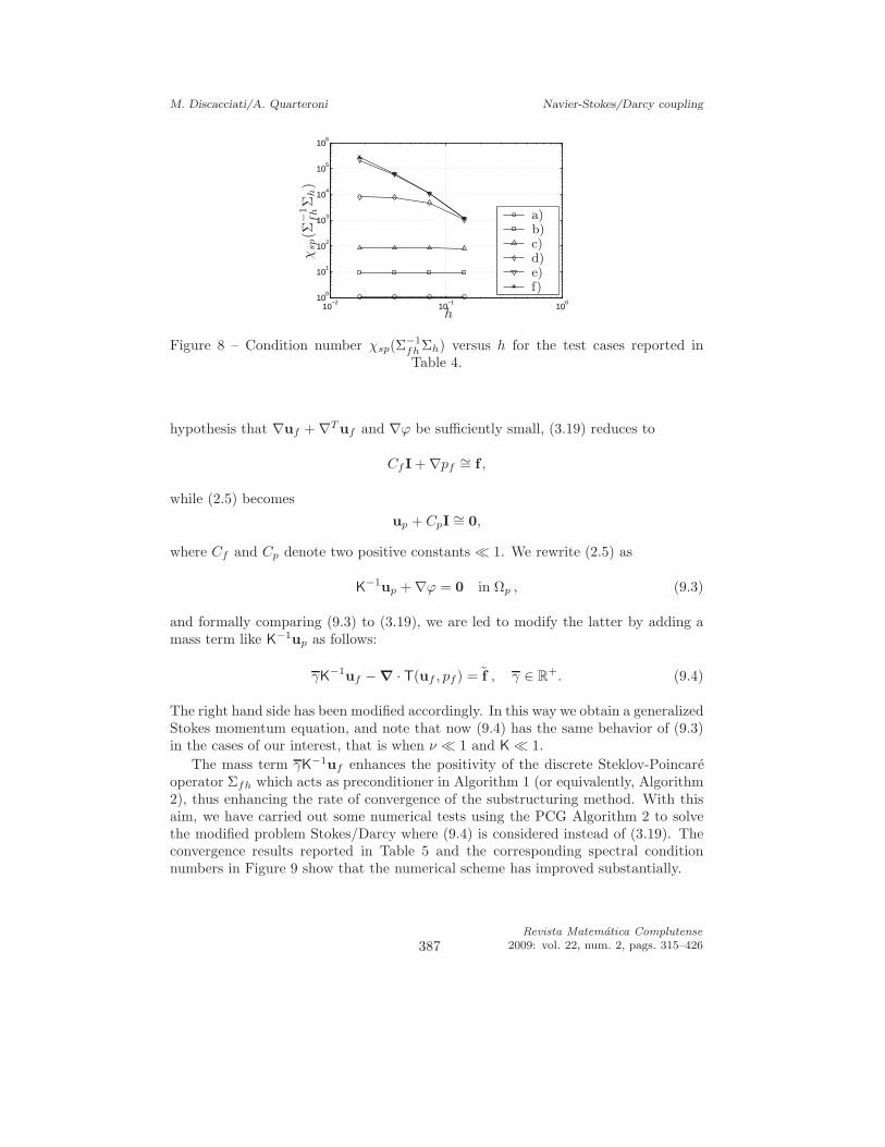
M. Discacciati/A. Quarteroni Navier-Stokes/Darcy coupling
10−2
10−1
100
100
101
102
103
104
105
106
hχ
sp(Σ
−1
fhΣ
h)
a)b)c)d)e)f)
Figure 8 – Condition number χsp(Σ−1fh Σh) versus h for the test cases reported inTable 4.
hypothesis that ∇uf + ∇Tuf and ∇ϕ be sufficiently small, (3.19) reduces to
Cf I + ∇pf∼= f ,
while (2.5) becomes
up + CpI ∼= 0,
where Cf and Cp denote two positive constants ≪ 1. We rewrite (2.5) as
K−1up + ∇ϕ = 0 in Ωp , (9.3)
and formally comparing (9.3) to (3.19), we are led to modify the latter by adding amass term like K
−1up as follows:
γK−1uf − ∇ · T(uf , pf) = f , γ ∈ R+. (9.4)
The right hand side has been modified accordingly. In this way we obtain a generalizedStokes momentum equation, and note that now (9.4) has the same behavior of (9.3)in the cases of our interest, that is when ν ≪ 1 and K ≪ 1.
The mass term γK−1uf enhances the positivity of the discrete Steklov-Poincareoperator Σfh which acts as preconditioner in Algorithm 1 (or equivalently, Algorithm2), thus enhancing the rate of convergence of the substructuring method. With thisaim, we have carried out some numerical tests using the PCG Algorithm 2 to solvethe modified problem Stokes/Darcy where (9.4) is considered instead of (3.19). Theconvergence results reported in Table 5 and the corresponding spectral conditionnumbers in Figure 9 show that the numerical scheme has improved substantially.
387Revista Matematica Complutense
2009: vol. 22, num. 2, pags. 315–426
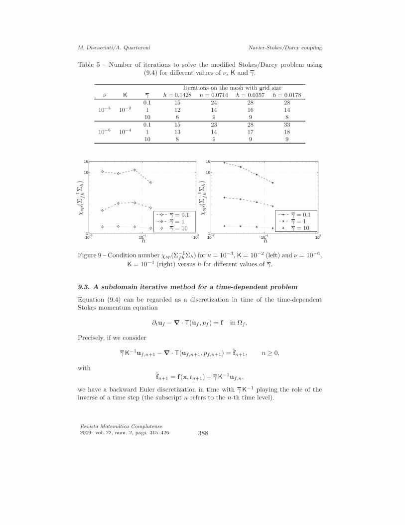
M. Discacciati/A. Quarteroni Navier-Stokes/Darcy coupling
Table 5 – Number of iterations to solve the modified Stokes/Darcy problem using(9.4) for different values of ν, K and γ.
Iterations on the mesh with grid sizeν K γ h = 0.1428 h = 0.0714 h = 0.0357 h = 0.0178
0.1 15 24 28 2810−3 10−2 1 12 14 16 14
10 8 9 9 8
0.1 15 23 28 3310−6 10−4 1 13 14 17 18
10 8 9 9 9
10−2
10−1
100
1
10
15
h
χsp(Σ
−1
fhΣ
h)
γ = 0.1γ = 1γ = 10
10−2
10−1
100
1
10
15
h
χsp(Σ
−1
fhΣ
h)
γ = 0.1γ = 1γ = 10
Figure 9 – Condition number χsp(Σ−1fhΣh) for ν = 10−3, K = 10−2 (left) and ν = 10−6,
K = 10−4 (right) versus h for different values of γ.
9.3. A subdomain iterative method for a time-dependent problem
Equation (9.4) can be regarded as a discretization in time of the time-dependentStokes momentum equation
∂tuf − ∇ · T(uf , pf ) = f in Ωf .
Precisely, if we consider
γ K−1uf,n+1 − ∇ · T(uf,n+1, pf,n+1) = fn+1, n ≥ 0,
with
fn+1 = f(x, tn+1) + γ K−1uf,n,
we have a backward Euler discretization in time with γ K−1 playing the role of the
inverse of a time step (the subscript n refers to the n-th time level).
Revista Matematica Complutense
2009: vol. 22, num. 2, pags. 315–426 388
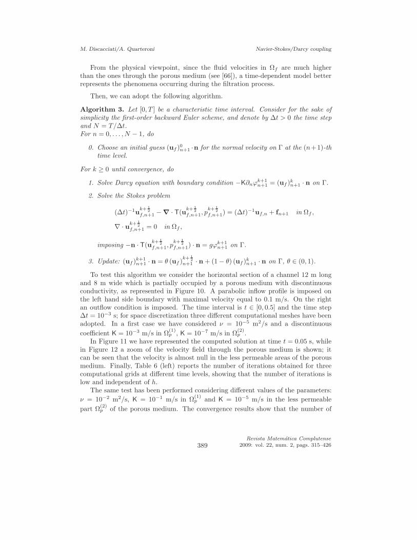
M. Discacciati/A. Quarteroni Navier-Stokes/Darcy coupling
From the physical viewpoint, since the fluid velocities in Ωf are much higherthan the ones through the porous medium (see [66]), a time-dependent model betterrepresents the phenomena occurring during the filtration process.
Then, we can adopt the following algorithm.
Algorithm 3. Let [0, T ] be a characteristic time interval. Consider for the sake ofsimplicity the first-order backward Euler scheme, and denote by ∆t > 0 the time stepand N = T/∆t.For n = 0, . . . , N − 1, do
0. Choose an initial guess (uf )0n+1 ·n for the normal velocity on Γ at the (n+1)-thtime level.
For k ≥ 0 until convergence, do
1. Solve Darcy equation with boundary condition −K∂nϕk+1n+1 = (uf )k
n+1 · n on Γ.
2. Solve the Stokes problem
(∆t)−1uk+ 1
2
f,n+1 − ∇ · T(uk+ 1
2
f,n+1, pk+ 1
2
f,n+1) = (∆t)−1uf,n + fn+1 in Ωf ,
∇ · uk+ 1
2
f,n+1 = 0 in Ωf ,
imposing −n · T(uk+ 1
2
f,n+1, pk+ 1
2
f,n+1) · n = gϕk+1n+1 on Γ.
3. Update: (uf )k+1n+1 · n = θ (uf )
k+ 1
2
n+1 · n + (1 − θ) (uf )kn+1 · n on Γ, θ ∈ (0, 1).
To test this algorithm we consider the horizontal section of a channel 12 m longand 8 m wide which is partially occupied by a porous medium with discontinuousconductivity, as represented in Figure 10. A parabolic inflow profile is imposed onthe left hand side boundary with maximal velocity equal to 0.1 m/s. On the rightan outflow condition is imposed. The time interval is t ∈ [0, 0.5] and the time step∆t = 10−3 s; for space discretization three different computational meshes have beenadopted. In a first case we have considered ν = 10−5 m2/s and a discontinuous
coefficient K = 10−3 m/s in Ω(1)p , K = 10−7 m/s in Ω
(2)p .
In Figure 11 we have represented the computed solution at time t = 0.05 s, whilein Figure 12 a zoom of the velocity field through the porous medium is shown; itcan be seen that the velocity is almost null in the less permeable areas of the porousmedium. Finally, Table 6 (left) reports the number of iterations obtained for threecomputational grids at different time levels, showing that the number of iterations islow and independent of h.
The same test has been performed considering different values of the parameters:
ν = 10−2 m2/s, K = 10−1 m/s in Ω(1)p and K = 10−5 m/s in the less permeable
part Ω(2)p of the porous medium. The convergence results show that the number of
389Revista Matematica Complutense
2009: vol. 22, num. 2, pags. 315–426
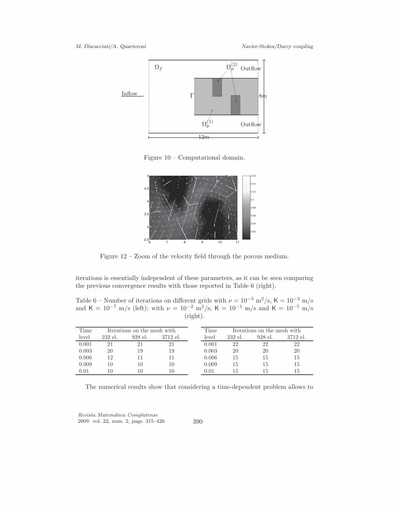
M. Discacciati/A. Quarteroni Navier-Stokes/Darcy coupling
Inflow
Outflow
Outflow
12m
8mΓ
Ωf Ω(2)p
Ω(1)p
Figure 10 – Computational domain.
0.02
0.04
0.06
0.08
0.1
0.12
0.14
0.16
6 7 8 9 10 112.5
3
3.5
4
4.5
5
Figure 12 – Zoom of the velocity field through the porous medium.
iterations is essentially independent of these parameters, as it can be seen comparingthe previous convergence results with those reported in Table 6 (right).
Table 6 – Number of iterations on different grids with ν = 10−5 m2/s, K = 10−3 m/sand K = 10−7 m/s (left); with ν = 10−2 m2/s, K = 10−1 m/s and K = 10−5 m/s
(right).
Time Iterations on the mesh withlevel 232 el. 928 el. 3712 el.0.001 21 21 210.003 20 19 190.006 12 11 110.009 10 10 100.01 10 10 10
Time Iterations on the mesh withlevel 232 el. 928 el. 3712 el.0.001 22 22 220.003 20 20 200.006 15 15 150.009 15 15 150.01 15 15 15
The numerical results show that considering a time-dependent problem allows to
Revista Matematica Complutense
2009: vol. 22, num. 2, pags. 315–426 390
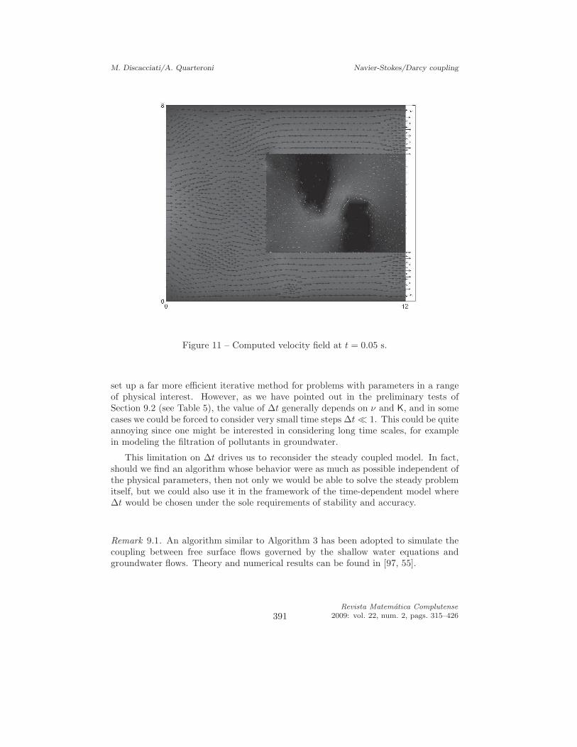
M. Discacciati/A. Quarteroni Navier-Stokes/Darcy coupling
Figure 11 – Computed velocity field at t = 0.05 s.
set up a far more efficient iterative method for problems with parameters in a rangeof physical interest. However, as we have pointed out in the preliminary tests ofSection 9.2 (see Table 5), the value of ∆t generally depends on ν and K, and in somecases we could be forced to consider very small time steps ∆t≪ 1. This could be quiteannoying since one might be interested in considering long time scales, for examplein modeling the filtration of pollutants in groundwater.
This limitation on ∆t drives us to reconsider the steady coupled model. In fact,should we find an algorithm whose behavior were as much as possible independent ofthe physical parameters, then not only we would be able to solve the steady problemitself, but we could also use it in the framework of the time-dependent model where∆t would be chosen under the sole requirements of stability and accuracy.
Remark 9.1. An algorithm similar to Algorithm 3 has been adopted to simulate thecoupling between free surface flows governed by the shallow water equations andgroundwater flows. Theory and numerical results can be found in [97, 55].
391Revista Matematica Complutense
2009: vol. 22, num. 2, pags. 315–426
M. Discacciati/A. Quarteroni Navier-Stokes/Darcy coupling
10. Robin-Robin methods for the Stokes/Darcy coupling
In this section, we consider iterative methods to solve the Stokes/Darcy problem(4.13)–(4.14) based on Robin conditions across the interface Γ, i.e., proper linearcombinations of the coupling conditions (3.16) and (3.17). These methods extendthose illustrated in Section 8 and they are more robust giving a convergence rate thatwe observed numerically to be essentially independent of the grid parameter h and ofthe physical quantities characterizing the filtration.
We point out that these methods and their algebraic interpretation (see [53, 54])have inspired algorithms featuring a similar structure in the context of fluid-structureinteractions between blood flows and the poroelastic arterial wall. We refer the readerto [15] and also to [107, Chapter 6].
For the sake of simplicity, in the rest of this section we will consider the simpli-fied condition on the interface uf · τ j = 0 instead of (3.18). Moreover, we will usehomogeneous boundary conditions, i.e., we will set uin = 0 in (4.2) and ϕp = 0 in(4.3).
10.1. A sequential Robin-Robin (sRR) method
We consider a sequential Robin-Robin (sRR) method which at each iteration requiresto solve a Darcy problem in Ωp followed by a Stokes problem in Ωf , both with Robinconditions on Γ. Precisely, the algorithm reads as follows.
Having assigned a trace function η0 ∈ L2(Γ), and two acceleration parametersγf ≥ 0 and γp > 0, for each k ≥ 0:
(i) Find ϕk+1 ∈ Hp such that
γpap(ϕk+1, ψ) +
∫
Γ
gϕk+1|Γ ψ|Γ =
∫
Γ
ηkψ|Γ ∀ ψ ∈ Hp . (10.1)
This corresponds to imposing the following interface condition (in weak, ornatural, form) for the Darcy problem:
−γpK∂nϕk+1 + gϕk+1
|Γ = ηk on Γ . (10.2)
(ii) Then, find (uk+1f , pk+1
f ) ∈ Hτf ×Q such that
af (uk+1f ,v) + bf (v, pk+1
f ) + γf
∫
Γ
(uk+1f · n)(v · n)
=
∫
Γ
(γf
γpηk − γf + γp
γpgϕk+1
|Γ
)
(v · n) +
∫
Ωf
f v ∀ v ∈ Hτf , (10.3)
bf(uk+1f , q) = 0 ∀ q ∈ Q . (10.4)
Revista Matematica Complutense
2009: vol. 22, num. 2, pags. 315–426 392
M. Discacciati/A. Quarteroni Navier-Stokes/Darcy coupling
This corresponds to imposing on the Stokes problem the following matchingconditions on Γ (still in natural form):
n · T(uk+1f , pk+1
f ) · n + γfuk+1f · n =
γf
γpηk − γf + γp
γpgϕk+1
|Γ
= −gϕk+1|Γ − γfK∂nϕ
k+1 (10.5)
uk+1f · τ j = 0, j = 1, . . . , d− 1.
(iii) Finally, set
ηk+1 = − n · T(uk+1f , pk+1
f ) · n + γpuk+1f · n
=(γf + γp)(uk+1f · n) +
γf + γp
γpgϕk+1
|Γ − γf
γpηk ∈ L2(Γ). (10.6)
Concerning the solvability of problem (10.3)–(10.4), we note first that using thetrace theorem and the Korn inequality (4.19), there exist two constants κ1, κ2 > 0such that
∫
Γ
|uf · n|2 ≤ κ1
(
∫
Ωf
(|uf |2 + |∇uf |2))
≤ κ2
∫
Ωf
|∇uf + ∇T uf |2 .
Therefore, the bilinear form
af (uf ,v) + γf
∫
Γ
(uf · n)(v · n)
is continuous and coercive in Hτf ×Hτ
f . Moreover, the bilinear form bf(v, p) satisfiesan inf–sup condition on the space Hτ
f ×Q (see, e.g., [110, pages 157–158]). Then, for
every f ∈ (L2(Ωf ))d, ηk ∈ L2(Γ) and ϕk+1|Γ ∈ L2(Γ), there exists a unique solution of
problem (10.3)–(10.4).
If the sRR method converges, in the limit we recover the solution (uf , pf) ∈ Hτf ×Q
and ϕ ∈ Hp of the coupled Stokes/Darcy problem. Indeed, denoting by ϕ∗ the limitof the sequence ϕk in H1(Ωp) and by (u∗
f , p∗f) that of (uk
f , pkf) in (H1(Ωf ))d ×Q, we
obtain−γpK∇ϕ∗ · n + gϕ∗
|Γ = −n · T(u∗f , p
∗f) · n + γpu
∗f · n on Γ , (10.7)
so that, as a consequence of (10.5), we have
(γf + γp)u∗f · n = −(γf + γp)K∇ϕ∗ · n on Γ ,
yielding, since γf + γp 6= 0, u∗f · n = −K∂nϕ
∗ on Γ, and also, from (10.7), thatn ·T(u∗
f , p∗f)·n = −gϕ∗
|Γ on Γ. Thus, the two interface conditions (3.16) and (3.17) are
satisfied, and we can conclude that the limit functions ϕ∗ ∈ Hp and (u∗f , p
∗f ) ∈ Hτ
f ×Qare the solutions of the coupled Stokes/Darcy problem.
We address the issue of convergence of the sRR method in Section 10.3.
393Revista Matematica Complutense
2009: vol. 22, num. 2, pags. 315–426
M. Discacciati/A. Quarteroni Navier-Stokes/Darcy coupling
10.2. Interpretation of the sRR method as an alternating direction scheme
The sRR method can be interpreted as an alternating direction scheme (see [8] andalso [53]). For technical reasons, to make precise this statement let us assume thatthe flux boundary condition T(uf , pf) ·n = 0 is imposed on the top Γ2
f (see Figure 1)of the fluid domain Ωf . This allows us to guarantee at each step the uniqueness ofthe pressure pf in the space Q. Moreover, we assume that the interface Γ is smooth,say, a C2-manifold with boundary. Then, we introduce the spaces Hf = v ∈ (H1(Ωf ))d : v = 0 on Γ1
f ∪ Γ3f, Hτ
f = v ∈ Hf : v · τ j = 0 on Γ, j = 1, . . . , d− 1, Hτ,nf = v ∈ Hτ
f : v · n = 0 on Γ,
and we define the operator ÒSf asÒSf : H1/200 (Γ) → (H
1/200 (Γ))′, χ→ ÒSfχ = n · (T(uχ, pχ) · n),
where (uχ, pχ) ∈ Hτf ×Q satisfies
af (uχ,v) + bf (v, pχ) = 0 ∀ v ∈ Hτ,nf (Ωf ) ,
bf (uχ, q) = 0 ∀ q ∈ Q ,
with uχ · n = χ on Γ.
Notice that ÒSf corresponds essentially to the operator Sf defined in (5.17) exceptfor the boundary condition T(uf , pf) · n = 0 on Γ2
f . Indeed, in the definition of Sf
only homogeneous Dirichlet boundary conditions on ∂Ωf \ Γ were imposed.On the other hand, let Sp be the operator defined in (5.18). Let us recall that, for
each η ∈ (H1/200 (Γ))′,
Sp : (H1/200 (Γ))′ → H
1/200 (Γ), η → Spη = gϕη|Γ,
where ϕη ∈ Hp is the solution of
ap(ϕη, ψ) = 〈η, ψ|Γ〉Γ ∀ ψ ∈ Hp ,
and 〈·, ·〉Γ denotes the duality pairing between (H1/200 (Γ))′ and H
1/200 (Γ). As a conse-
quence, we have −K∂nϕη = η on Γ.Since for each ϕ ∈ Hp we have Sp(−K∂nϕ) = gϕ|Γ, the first step (10.3)–(10.4) of
our procedure corresponds to imposing on Γ
−γpK∂nϕk+1 + gϕk+1
|Γ = −γpK∇ϕk+1 · n + Sp(−K∂nϕk+1)
= (γpI + Sp)(−K∂nϕk+1) = ηk ,
Revista Matematica Complutense
2009: vol. 22, num. 2, pags. 315–426 394
M. Discacciati/A. Quarteroni Navier-Stokes/Darcy coupling
hence−K∂nϕ
k+1 = (γpI + Sp)−1ηk .
On the other hand, the right hand side in (10.5) can be written as
−gϕk+1|Γ − γfK∂nϕ
k+1 =Sp(K∂nϕk+1) − γfK∂nϕ
k+1
= − (γfI − Sp)K∂nϕk+1
=(γf I − Sp)(γpI + Sp)−1ηk . (10.8)
In an analogous way, still denoting by (uk+1f , pk+1
f ) the solution of (10.3)–(10.4)
with f = 0 and Hτf replaced by Hτ
f , one has ÒSf (uk+1f · n) = n · T(uk+1
f , pk+1f ) · n.
Then, the left hand side in (10.5) can be written as
n · T(uk+1, pk+1) · n + γfuk+1 · n = ÒSf (uk+1 · n) + γfu
k+1 · n= (γf I + ÒSf )(uk+1 · n) . (10.9)
Using (10.8) and (10.9), the interface condition (10.5) becomes
uk+1 · n = (γfI + ÒSf )−1(γfI − Sp)(γpI + Sp)−1ηk .
In conclusion, our iterative procedure (with f = 0) can be written as
ηk+1 = −n · T(uk+1, pk+1 · n) + γpuk+1 · n
= −ÒSf(uk+1 · n) + γpuk+1 · n
= (γpI − ÒSf )uk+1 · n= (γpI − ÒSf )(γf I + ÒSf )−1(γf I − Sp)(γpI + Sp)
−1ηk . (10.10)
This is an alternating direction scheme, a la Peaceman–Rachford (see [106]), thathas been deeply analyzed in the literature. Sufficient conditions for convergence arethat γf = γp and the operators ÒSf and Sp are bounded and strictly positive in a
given Hilbert space. These do not apply in the present situation, as the operators ÒSf
and Sp act from a space into its dual. In fact, we can only prove that the iteration
operator is non-expansive, but not a contraction in (H1/200 (Γ))′.
On the other hand, it is worthy to note that the convergence of this alternatingdirection scheme can be easily proved in the discrete case, as the matrices that cor-respond to the finite dimensional Steklov–Poincare operators ÒSf and Sp are in factsymmetric and positive definite. Indeed, the discrete counterpart of Sp is the local
Schur complement Σp introduced in (8.18), while ÒSf corresponds to a slight modifi-cation of Σf in (8.17) to account for the boundary condition T(uf , pf) ·n = 0 insteadof uf = 0 on Γ2
f .The prove of convergence of (10.10) can be found in [57].
395Revista Matematica Complutense
2009: vol. 22, num. 2, pags. 315–426
M. Discacciati/A. Quarteroni Navier-Stokes/Darcy coupling
10.3. Convergence of the sRR method
We prove that the sequences ϕk and (ukf , p
kf ) generated by the sRR method (10.1)–
(10.6) converge in H1(Ωp) and (H1(Ωf ))d × Q, respectively. As a consequence, thesequence ηk is convergent in the dual spaceH−1/2(Γ) and weakly convergent in L2(Γ).
The proof of convergence that we are presenting follows the guidelines of the theoryby P.-L. Lions [91] for the Robin-Robin method (see also [110, Section 4.5]).
We denote by eku = uk
f − uf , ekp = pk
f − pf and ekϕ = ϕk − ϕ the errors at the
k-th step. Remark that, thanks to the linearity, the functions (eku, e
kp) satisfy problem
(10.3)–(10.4) with f = 0, while ekϕ is a solution to (10.3)–(10.4). Moreover, we assume
that γp = γf , and we denote by γ their common value.Finally, let us point out that the solutions (uf , pf ) ∈ Hτ
f ×Q and ϕ ∈ Hp of the
coupled Stokes/Darcy problem satisfy n · T(uf , pf ) · n ∈ H1/2(Γ) (as it is equal to−gϕ|Γ on Γ), and ∇ϕ · n ∈ L2(Γ) (as it is equal to −K
−1uf · n on Γ), i.e., thesefunctions enjoy a better regularity than one might usually expect. Therefore, theinterface conditions (10.2) and (10.5) for the error functions hold in L2(Γ).
Let us come to the proof of convergence. Choosing ψ = ek+1ϕ in (10.1), and using
the identity
AB =1
4[(A+B)2 − (A−B)2] ,
we have
g ap(ek+1ϕ , ek+1
ϕ ) =1
γ
∫
Γ
(ηk − gek+1ϕ|Γ )gek+1
ϕ|Γ
=1
4γ
∫
Γ
(ηk)2 − 1
4γ
∫
Γ
(ηk − 2gek+1ϕ|Γ )2 . (10.11)
Similarly, taking v = ek+1u in (10.3) and using (10.6) we have:
af (ek+1u , ek+1
u ) =1
γ
∫
Γ
(ηk − 2gek+1ϕ|Γ − γek+1
u · n)(γek+1u · n)
=1
4γ
∫
Γ
(ηk − 2gek+1ϕ|Γ )2 − 1
4γ
∫
Γ
(ηk − 2gek+1ϕ|Γ − 2γek+1
u · n)2
=1
4γ
∫
Γ
(ηk − 2gek+1ϕ|Γ )2 − 1
4γ
∫
Γ
(ηk+1)2 . (10.12)
Adding (10.11) and (10.12) we find
g ap(ek+1ϕ , ek+1
ϕ ) + af (ek+1u , ek+1
u ) +1
4γ
∫
Γ
(ηk+1)2 =1
4γ
∫
Γ
(ηk)2 .
Summing over k from k = 0 to k = N , with N ≥ 1, we finally obtain
N∑
k=0
(
g ap(ek+1ϕ , ek+1
ϕ ) + af (ek+1u , ek+1
u ))
+1
4γ
∫
Γ
(ηN+1)2 =1
4γ
∫
Γ
(η0)2.
Revista Matematica Complutense
2009: vol. 22, num. 2, pags. 315–426 396
M. Discacciati/A. Quarteroni Navier-Stokes/Darcy coupling
Thus, the series∞∑
k=0
(
g ap(ek+1ϕ , ek+1
ϕ ) + af (ek+1u , ek+1
u ))
is convergent, and the errors ekϕ and ek
u tend to zero in H1(Ωp) and (H1(Ωf ))d,
respectively. The convergence of the pressure error ekp to 0 in Q is then a well-known
consequence of the convergence of the velocity.
10.4. Some numerical results
The sRR algorithm on the discrete problem (5.8)–(5.12) becomes: taking a tracefunction η0
h ∈ Λh, and considering two acceleration parameters γf ≥ 0 and γp > 0,for each k ≥ 0,
(i) Find ϕk+1h ∈ Hph such that
γpap(ϕk+1h , ψh) +
∫
Γ
gϕk+1h|Γ ψh|Γ =
∫
Γ
ηkhψh|Γ ∀ ψh ∈ Hph . (10.13)
(ii) Then, find (uk+1fh , pk+1
fh ) ∈ Hτfh ×Qh such that
af (uk+1fh ,vh) + bf (vh, p
k+1fh ) + γf
∫
Γ
(uk+1fh · n)(vh · n)
=
∫
Γ
(γf
γpηk
h − γf + γp
γpgϕk+1
h|Γ
)
(vh · n) +
∫
Ωf
f · vh ∀ vh ∈ Hτfh,
bf (uk+1fh , qh) = 0 ∀ qh ∈ Qh .
(10.14)
(iii) Finally, set
ηk+1h = (γf + γp)(u
k+1fh · n) +
γf + γp
γpgϕk+1
h|Γ − γf
γpηk
h ∈ Λh .
For γp = γf , the convergence of this algorithm can be proved as we did in Sec-tion 10.3 to show the convergence of (10.1)–(10.5). Moreover, it is also possible toprove the convergence of the alternating direction scheme (see Section 10.2), as thediscrete Steklov–Poincare operators are positive definite (however, in principle theproof of convergence cannot assure that the rate of convergence is independent of themesh size h).
For the numerical tests we have exploited the interpretation of the method in termsof alternating direction iterations (Section 10.2) in order to obtain some guidelines forthe choice of the relaxation parameters, at least for the case of our interest, that is,when ν and the entries of K are very small (we recall that in this case the convergencerate of the Dirichlet-Neumann method deteriorates, see Section 9.2).
397Revista Matematica Complutense
2009: vol. 22, num. 2, pags. 315–426
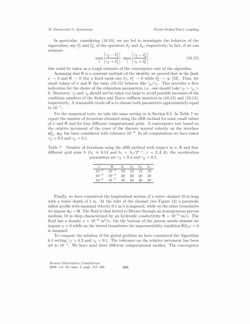
M. Discacciati/A. Quarteroni Navier-Stokes/Darcy coupling
In particular, considering (10.10), we are led to investigate the behavior of theeigenvalues, say δj
f and δjp, of the operators Sf and Sp, respectively; in fact, if we can
estimate
maxj
∣
∣
∣
∣
∣
γp − δjf
γf + δjf
∣
∣
∣
∣
∣
· maxj
∣
∣
∣
∣
∣
γf − δjp
γp + δjp
∣
∣
∣
∣
∣
, (10.15)
this could be taken as a rough estimate of the convergence rate of the algorithm.Assuming that K is a constant multiple of the identity, we proved that in the limit
ν → 0 and K → 0 (for a fixed mesh size h), δjf → 0 while δj
p → ∞ [53]. Thus, forsmall values of ν and K the ratio (10.15) behaves like γp/γf . This provides a firstindication for the choice of the relaxation parameters, i.e., one should take γf > γp >0. Moreover, γf and γp should not be taken too large to avoid possible increases of thecondition numbers of the Stokes and Darcy stiffness matrices in (10.13) and (10.14),respectively. A reasonable trade-off is to choose both parameters approximately equalto 10−1.
For the numerical tests, we take the same setting as in Section 9.2. In Table 7 wereport the number of iterations obtained using the sRR method for some small valuesof ν and K and for four different computational grids. A convergence test based onthe relative increment of the trace of the discrete normal velocity on the interfaceuk
fh ·n|Γ has been considered with tolerance 10−9. In all computations we have takenγf = 0.3 and γp = 0.1.
Table 7 – Number of iterations using the sRR method with respect to ν, K and fourdifferent grid sizes h (h1 ≈ 0.14 and hi = h1/2
i−1, i = 2, 3, 4); the accelerationparameters are γf = 0.3 and γp = 0.1.
ν K h1 h2 h3 h4
10−4 10−3 19 19 19 1910−6 10−4 20 20 20 2010−6 10−7 20 20 20 20
Finally, we have considered the longitudinal section of a water channel 10 m longwith a water depth of 1 m. At the inlet of the channel (see Figure 13) a parabolicinflow profile with maximal velocity 0.1 m/s is imposed, while on the other boundarieswe impose uf = 0. The fluid is thus forced to filtrate through an homogeneous porousmedium 10 m deep characterized by an hydraulic conductivity K = 10−3 m/s. Thefluid has a density ν = 10−6 m2/s. On the bottom of the porous media domain weimpose ϕ = 0 while on the lateral boundaries the impermeability condition K∂nϕ = 0is assumed.
To compute the solution of the global problem we have considered the Algorithm6.1 setting γf = 0.3 and γp = 0.1. The tolerance on the relative increment has beenset to 10−5. We have used three different computational meshes. The convergence
Revista Matematica Complutense
2009: vol. 22, num. 2, pags. 315–426 398
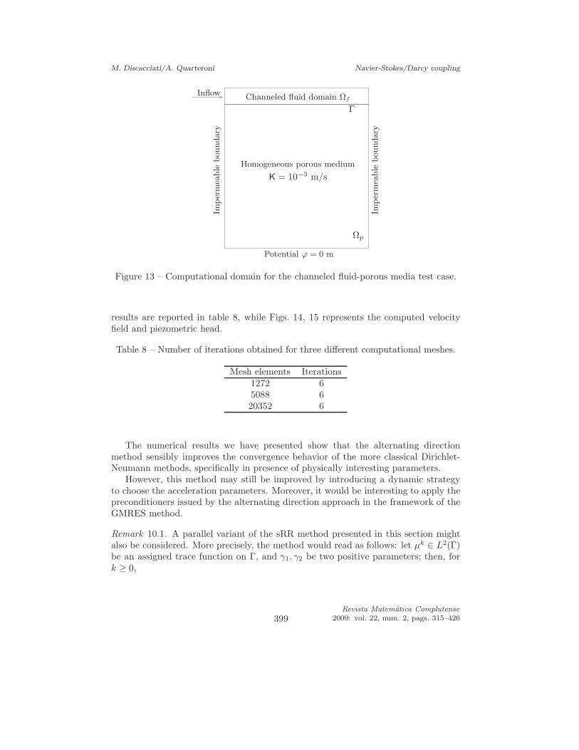
M. Discacciati/A. Quarteroni Navier-Stokes/Darcy coupling
Inflow
Γ
Ωp
Homogeneous porous medium
K = 10−3 m/s
Potential ϕ = 0 m
Imper
mea
ble
boundary
Imper
mea
ble
boundary
Channeled fluid domain Ωf
Figure 13 – Computational domain for the channeled fluid-porous media test case.
results are reported in table 8, while Figs. 14, 15 represents the computed velocityfield and piezometric head.
Table 8 – Number of iterations obtained for three different computational meshes.
Mesh elements Iterations1272 65088 620352 6
The numerical results we have presented show that the alternating directionmethod sensibly improves the convergence behavior of the more classical Dirichlet-Neumann methods, specifically in presence of physically interesting parameters.
However, this method may still be improved by introducing a dynamic strategyto choose the acceleration parameters. Moreover, it would be interesting to apply thepreconditioners issued by the alternating direction approach in the framework of theGMRES method.
Remark 10.1. A parallel variant of the sRR method presented in this section mightalso be considered. More precisely, the method would read as follows: let µk ∈ L2(Γ)be an assigned trace function on Γ, and γ1, γ2 be two positive parameters; then, fork ≥ 0,
399Revista Matematica Complutense
2009: vol. 22, num. 2, pags. 315–426
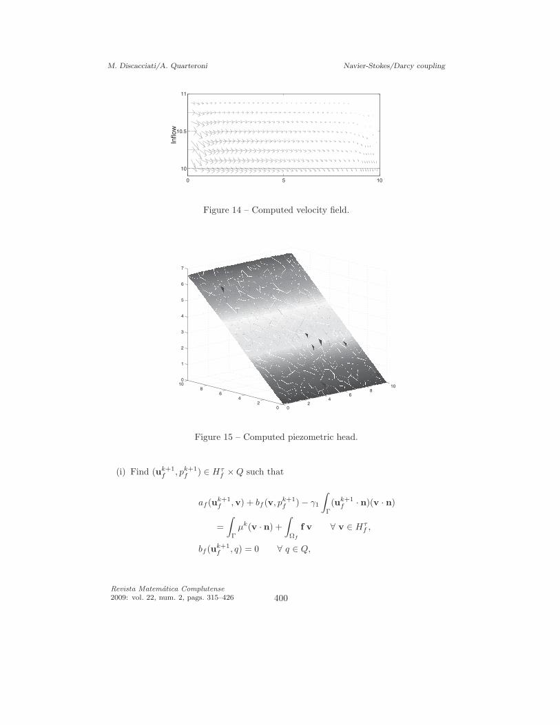
M. Discacciati/A. Quarteroni Navier-Stokes/Darcy coupling
0 5 10
10
10.5
11
Inflow
Figure 14 – Computed velocity field.
0
2
4
6
8
10
0
2
4
6
8
10
0
1
2
3
4
5
6
7
Figure 15 – Computed piezometric head.
(i) Find (uk+1f , pk+1
f ) ∈ Hτf ×Q such that
af (uk+1f ,v) + bf (v, pk+1
f ) − γ1
∫
Γ
(uk+1f · n)(v · n)
=
∫
Γ
µk(v · n) +
∫
Ωf
f v ∀ v ∈ Hτf ,
bf (uk+1f , q) = 0 ∀ q ∈ Q,
Revista Matematica Complutense
2009: vol. 22, num. 2, pags. 315–426 400
M. Discacciati/A. Quarteroni Navier-Stokes/Darcy coupling
and, at the same time, find ϕk+1 ∈ Hp such that
ap(ϕk+1, ψ) +
1
γ1
∫
Γ
gϕk+1|Γ ψ|Γ = − 1
γ1
∫
Γ
µkψ|Γ ∀ ψ ∈ Hp .
Remark that on the interface Γ we are imposing the matching conditions
n · T(uk+1f , pk+1) · n− γ1u
k+1f · n = µk= −gϕk+1
|Γ + γ1K∂nϕk+1,
uk+1f · τ j = 0, j = 1, . . . , d− 1.
(ii) As a second step, find (bωk+1, bπk+1) ∈ Hτf ×Q such that
af (bωk+1,v) + bf(v, bπk+1) + γ2
∫
Γ
(bωk+1 · n)(v · n)
= γ2
∫
Γ
bσk+1(v · n) ∀ v ∈ Hτf ,
bf (bωk+1, q) = 0 ∀ q ∈ Q ,
and find bχk+1 ∈ Hp such that
ap(bχk+1, ψ) +1
γ2
∫
Γ
gbχk+1|Γ ψ|Γ =
∫
Γ
bσk+1ψ|Γ ∀ ψ ∈ Hp ,
wherebσk+1 = uk+1f · n + K∂nϕ
k+1 = uk+1f · n +
1
γ1(gϕk+1
|Γ + µk) ∈ L2(Γ) .
Note that on the interface Γ we are now imposing the matching conditions
n · T(bωk+1, bπk+1) · n + γ2bωk+1 · n = γ2bσk+1 = gbχk+1|Γ − γ2K∂nbχk+1,bωk+1 · τ j = 0, j = 1, . . . , d− 1.
(iii) Finally, set
µk+1 = µk − θ[n · T(bωk+1, bπk+1) · n + gbχk+1|Γ ]
= µk − θ[γ2(bσk+1 − bωk+1 · n) + gbχk+1|Γ ] ∈ L2(Γ) ,
where θ > 0 is a further acceleration parameter.
Although interesting from the theoretical point of view this algorithm unfortu-nately yields poor convergence results. We refer the reader to [57].
401Revista Matematica Complutense
2009: vol. 22, num. 2, pags. 315–426
M. Discacciati/A. Quarteroni Navier-Stokes/Darcy coupling
11. Iterative methods for the Navier-Stokes/Darcy problem
In this section, we introduce and analyze some iterative methods to compute the solu-tion of a conforming finite element approximation of the non-linear Navier-Stokes/Dar-cy problem (4.11)–(4.12). For the easiness of notation, we will write our algorithmsin continuous form. However, they can be straightforwardly translated into a discretesetting considering conforming internal Galerkin approximations of the spaces usedhereafter.
Moreover, the convergence results that we will present hold in the discrete case(i.e., in the finite element spaces) without any dependence of the convergence rateon the grid parameter h, since they are established by using the properties of theoperators in the continuous case.
Finally, for the sake of simplicity, we adopt homogeneous boundary conditions asalready done in Section 6.
11.1. Fixed-point iterations
Fixed-point iterations to solve the coupled problem (4.11)–(4.12) can be written asfollows. Given u0
f ∈ Hf , for n ≥ 1, find unf ∈ Hf , pn
f ∈ Q, ϕn ∈ Hp such that
af (unf ,v) + cf (un−1
f ;unf ,v) + bf (v, pn
f )
+
∫
Γ
g ϕn(v · n) +
∫
Γ
d−1∑
j=1
ναBJ√K
(unf · τ j)(v · τ j) =
∫
Ωf
f v , (11.1)
bf (unf , q) = 0 , (11.2)
ap(ϕn, ψ) =
∫
Γ
ψ(unf · n) , (11.3)
for all v ∈ Hf , q ∈ Q, ψ ∈ Hp.
Algorithm (11.1)–(11.3) requires to solve at each iteration a linear coupled prob-lem, and it can be reinterpreted as a fixed-point method to solve the interface problem(6.25). Indeed, let us first rewrite (11.1)–(11.2) in the equivalent form:
find unf ∈ Vf such that
af (unf ,v) + cf (un−1
f ;unf ,v) +
∫
Γ
g ϕn(v · n)
+
∫
Γ
d−1∑
j=1
ναBJ√K
(unf · τ j)(v · τ j) =
∫
Ωf
f v ∀v ∈ Vf . (11.4)
We denote λn = unf · n on Γ and we remark that λn ∈ Λ0. Then, we considerÜR1
fλn ∈ Hf and we set un = un
f − ÜR1fλ
n. By definition, un · n = 0 on Γ. Moreover,
Revista Matematica Complutense
2009: vol. 22, num. 2, pags. 315–426 402
M. Discacciati/A. Quarteroni Navier-Stokes/Darcy coupling
remark that for all η ∈ Λ0, (6.8) implies that ∇ · ÜR1fη = 0 in Ωf since we can choose
q = ∇ · ÜR1fη. Thus, un ∈ V 0
f .
From (11.3) it follows −K∂nϕn = un
f · n = λn on Γ, so that by definition of Rp,we can write ϕn = Rpλ
n.
Finally, since v ∈ Vf , proceeding as for unf , we can split v = w+ÜR1
fµ with µ = v·non Γ and w ∈ V 0
f . Thus, (11.4) becomes
af (un + ÜR1fλ
n,w + ÜR1fµ) + cf (un−1 + ÜR1
fλn−1;un + ÜR1
fλn,w + ÜR1
fµ)
+
∫
Γ
g(Rpλn)(w + ÜR1
fµ) · n +
∫
Γ
d−1∑
j=1
ναBJ√K
((un + ÜR1fλ
n) · τ j) ((w + ÜR1fµ) · τ j)
=
∫
Ωf
f(w + ÜR1fµ) .
Taking into account that w ∈ V 0f and the definition of ÜR1
f (6.7)–(6.8), this correspondsto the fixed-point method:
Given un−1 = (λn−1,un−1) ∈ W , for n ≥ 1,
find un = (λn,un) ∈ W : a(un−1; un, w) = 〈ℓ, w〉 ∀w = (µ,w) ∈ W .
(Recall that W = Λ0 × V 0f . See Section 6.2.)
Thanks to this equivalence, the convergence of (11.1)–(11.3) is a direct consequenceof Lemma 6.5. We can state the following result which is a straightforward corollaryof Theorem 6.7.
Proposition 11.1. If (6.26) holds and if u0f is such that the H1 seminorm in Ωf
|ÜR1f (u0
f · n)|1 < rM with rM given in (6.27), then the sequence (unf , p
nf , ϕ
n) converges
for n → ∞ to the unique solution (uf , pf , ϕ) of problem (4.11)–(4.12), and |ÜR1f (uf ·
n)|1 ≤ rm.
11.2. Newton-like methods
Let us consider now the following Newton method to solve (the discrete form of)(4.11)–(4.12): let u0
f ∈ Hf be given; then, for n ≥ 1, find unf ∈ Hf , pn
f ∈ Q, ϕn ∈ Hp
403Revista Matematica Complutense
2009: vol. 22, num. 2, pags. 315–426
M. Discacciati/A. Quarteroni Navier-Stokes/Darcy coupling
such that, for all v ∈ Hf , q ∈ Q, ψ ∈ Hp,
af(unf ,v) + cf (un
f ;un−1f ,v) + cf (un−1
f ;unf ,v) + bf (v, pn
f ) +
∫
Γ
gϕn(v · n)
+
∫
Γ
d−1∑
j=1
ναBJ√K
(unf · τ j)(v · τ j) = cf(un−1
f ;un−1f ,v) +
∫
Ωf
f v , (11.5)
bf(unf , q) = 0 , (11.6)
ap(ϕn, ψ) =
∫
Γ
ψ(unf · n) . (11.7)
In order to reduce the computational cost, we might consider the modified Newtonmethod:
find unf ∈ Hf , pn
f ∈ Q, ϕn ∈ Hp such that, for all v ∈ Hf , q ∈ Q, ψ ∈ Hp,
af (unf ,v) + cf (un
f ;u0f ,v) + cf (u0
f ;unf ,v) + bf(v, pn
f ) +
∫
Γ
gϕn(v · n)
+
∫
Γ
d−1∑
j=1
ναBJ√K
(unf · τ j)(v · τ j) = cf (un−1
f ;u0f ,v)
+ cf (u0f − un−1
f ;un−1f ,v) +
∫
Ωf
f v , (11.8)
bf (unf , q) = 0 , (11.9)
ap(ϕn, ψ) =
∫
Γ
ψ(unf · n) . (11.10)
Like for fixed-point iterations, we have to solve a linearized coupled problem ateach iteration of the Newton algorithms.
This method corresponds to using an inexact Jacobian in which we have droppedthe terms arising from the linearized trilinear convective terms. The matrix associatedto this inexact Jacobian is now independent of the iteration level, hence it can befactorized once and for all (offline) at the very first iteration.
We would like to rewrite the Newton methods (11.5)–(11.7) and (11.8)–(11.10) asiterative schemes for the interface equation (6.25). Let us consider the exact Newtonmethod first. First of all, notice that it can be expressed in the equivalent form:
Revista Matematica Complutense
2009: vol. 22, num. 2, pags. 315–426 404
M. Discacciati/A. Quarteroni Navier-Stokes/Darcy coupling
find unf ∈ Vf , ϕn ∈ Hp such that, for all v ∈ Vf , ψ ∈ Hp,
af (unf ,v) + cf (un
f ;un−1f ,v) + cf (un−1
f ;unf ,v) +
∫
Γ
gϕn(v · n)
+
∫
Γ
d−1∑
j=1
ναBJ√K
(unf · τ j)(v · τ j) = cf (un−1
f ;un−1f ,v) +
∫
Ωf
f v , (11.11)
ap(ϕn, ψ) =
∫
Γ
ψ(unf · n) .
Furthermore, (11.11) can be equivalently restated as:
find unf ∈ Vf such that
af (unf − un−1
f ,v) + cf(unf − un−1
f ;un−1f ,v) + cf (un−1
f ;unf − un−1
f ,v)
+
∫
Γ
g(ϕn − ϕn−1)(v · n) +
∫
Γ
d−1∑
j=1
ναBJ√K
((unf − un−1
f ) · τ j)(v · τ j)
= −af(un−1f ,v) − cf (un−1
f ;un−1f ,v) −
∫
Γ
gϕn−1(v · n)
−∫
Γ
d−1∑
j=1
ναBJ√K
(un−1f · τ j)(v · τ j) +
∫
Ωf
f v ∀v ∈ Vf . (11.12)
Let us now indicate by P (u) the operator associated to (6.25): P (u) : W → W ′,P (u) = (Au)u − ℓ, u = (λ,u) ∈ W , A and ℓ being defined in Section 6.2. Moreprecisely,
〈P (u), w〉 = af (ÜR1fλ, ÜR1
fµ) + af (u,w) + cf (u + ÜR1fλ;u + ÜR1
fλ,w + ÜR1fµ)
+
∫
Γ
d−1∑
j=1
ναBJ√K
(ÜR1fλ · τ j)(ÜR1
fµ · τ j) +
∫
Γ
d−1∑
j=1
ναBJ√K
(u · τ j)(w · τ j)
+
∫
Γ
g(Rpλ)µ−∫
Ωf
f(w + ÜR1fµ) ∀w = (µ,w) ∈ W .
405Revista Matematica Complutense
2009: vol. 22, num. 2, pags. 315–426
M. Discacciati/A. Quarteroni Navier-Stokes/Darcy coupling
The Gateaux derivative of the operator P in u reads, ∀v = (η,v), w = (µ,w) ∈ W ,
〈(P ′(u))(v), w〉 = af (ÜR1fη, ÜR1
fµ) + af (v,w)
+cf (v + ÜR1fη;u + ÜR1
fλ,w + ÜR1fµ)
+cf (u + ÜR1fλ;v + ÜR1
fη,w + ÜR1fµ)
+
∫
Γ
d−1∑
j=1
ναBJ√K
(ÜR1fη · τ j)(ÜR1
fµ · τ j)
+
∫
Γ
d−1∑
j=1
ναBJ√K
(v · τ j)(w · τ j) +
∫
Γ
g(Rpη)µ .
Notice also that, in view of the definition of ÜR1f , we have
〈P (u), w〉 =af (u + ÜR1fλ,w + ÜR1
fµ) + cf (u + ÜR1fλ;u + ÜR1
fλ,w + ÜR1fµ)
+
∫
Γ
d−1∑
j=1
ναBJ√K
((u + ÜR1fλ) · τ j)((w + ÜR1
fµ) · τ j)
+
∫
Γ
g(Rpλ)µ−∫
Ωf
f(w + ÜR1fµ) ,
and
〈(P ′(u))(v), w〉 = af(v + ÜR1fη,w + ÜR1
fµ) + cf (v + ÜR1fη;u + ÜR1
fλ,w + ÜR1fµ)
+ cf (u + ÜR1fλ;v + ÜR1
fη,w + ÜR1fµ)
+
∫
Γ
d−1∑
j=1
ναBJ√K
((v + ÜR1fη) · τ j)((w + ÜR1
fµ) · τ j) +
∫
Γ
g(Rpη)µ .
Following the same argument used in Section 11.1, we can write in (11.12) ukf =
uk+ÜR1fλ
k with uk ∈ V 0f and λk = uk
f ·n on Γ, and we can set ϕk = Rpλk (k = n−1, n).
Moreover, using again the fact that Vf = V 0f + ÜR1
fµ : µ ∈ Λ0, we can write
v = w + ÜR1fµ for w ∈ V 0
f and µ = v · n ∈ Λ0 on Γ.Substituting into (11.12), we can easily see that it corresponds to the following
Newton method to solve (6.25): given u0 = (λ0,u0) ∈ W , for n ≥ 1, find un =(λn,un) ∈ W such that
〈(P ′(un−1))(un − un−1), w〉 = −〈P (un−1), w〉 ∀w = (µ,w) ∈ W . (11.13)
Proceeding in an analogous way, one can show that algorithm (11.8)–(11.10) cor-responds to the modified Newton method to solve (6.25): given u0 = (λ0,u
0) ∈ W ,
Revista Matematica Complutense
2009: vol. 22, num. 2, pags. 315–426 406
M. Discacciati/A. Quarteroni Navier-Stokes/Darcy coupling
for n ≥ 1, find un = (λn,un) ∈ W such that
〈(P ′(u0))(un − un−1), w〉 = −〈P (un−1), w〉 ∀w = (µ,w) ∈ W . (11.14)
Concerning the convergence of the Newton methods, we can prove the followingresult.
Proposition 11.2. Let f ∈ L2(Ωf ) and let
C1 =32CNCΩf
‖f‖0
(Cκν)2, C2 =
2√
2CΩf||f ||0
Cκν.
If
C1 ≤ 1
2, (11.15)
then, there exists a unique solution u = (λ,R10(λ)) ∈ Br0
of (6.25), with
Br0= w = (η,w) ∈ W : ‖w‖W ≤ r0 (11.16)
and
r0 =1 −
√
1 − 2C1
C1
C2 . (11.17)
Moreover, the sequence un = (λn,un), n ≥ 1, obtained by the Newton algorithms(11.13) or (11.14), taking u0 = (0,0) ∈ W, converges to this solution.
The following error estimate holds for the Newton method (11.13):
||u− un||W ≤ 1
2n(2C1)
2n C2
C1
, n ≥ 0, (11.18)
while for the modified Newton method (11.14) we have (if C1 < 1/2):
||u− un||W ≤ C2
C1
(
1 −√
1 − 2C1
)n+1
, n ≥ 0. (11.19)
Proof. The proof, which is a corollary of Theorem A.3, is given in [13]. We report ithere as well for sake of completeness. Consider u0 = (λ0,u0) = (0,0) ∈ W . Then, forall w = (η,w) ∈ W , we have:
〈(P ′(u0))(w), w〉 = af (ÜR1fη,ÜR1
fη) + af (w,w) +
∫
Γ
d−1∑
j=1
ναBJ√K
(ÜR1fη · τ j)(ÜR1
fη · τ j)
+
∫
Γ
d−1∑
j=1
ναBJ√K
(w · τ j)(w · τ j) +
∫
Γ
g(Rpη)η
≥ Cκν
2(|ÜR1
fη|21 + |w|21) =Cκν
2||w||2W .
407Revista Matematica Complutense
2009: vol. 22, num. 2, pags. 315–426
M. Discacciati/A. Quarteroni Navier-Stokes/Darcy coupling
Consequently, [P ′(u0)]−1 exists and
||[P ′(u0)]−1||L(W′,W) ≤2
Cκν.
Moreover,
〈P (u0), w〉 = −∫
Ωf
f(w + ÜR1fη) ≤
√2CΩf
‖f‖0||w||W ,
and therefore,||P (u0)||W′ ≤
√2CΩf
‖f‖0 .
The second derivative of the operator P reads:
〈((P ′′(u))(v))(w), ζ〉 = cf (w + ÜR1fη;v + ÜR1
fµ, z + ÜR1fξ)
+ cf (v + ÜR1fµ;w + ÜR1
fη, z + ÜR1fξ) ,
for u = (λ,u), v = (µ,v), w = (η,w), ζ = (ξ, z) ∈ W . Thus,
〈((P ′′(u))(v))(w), ζ〉 ≤ 2CN |w + ÜR1fη|1|v + ÜR1
fµ|1|z + ÜR1fξ|1
≤ 4√
2CN |v|W |w|W |ζ|W ,
so that||P ′′(u)||L(W,L(W,W′)) ≤ 4
√2CN .
Consequently, in our case, inequality (A.3) corresponds to (11.15).Moreover, since the operator P is defined and has continuous second derivative on
W , we can select a radius r satisfying (A.4)–(A.7) with r0 in (11.17) and
r1 =1 +
√
1 − 2C1
C1
C2 .
Finally, the error estimates (11.18) and (11.19) are directly obtained from (A.8) and(A.9), respectively.
Remark 11.3. With the help of a little algebra we can see that C1 and C2 are relatedto the constants C1 and C2 in (6.28) as: C1 = 2
√2C2/C1 and C2 = 2
√2C2
2/C1. Thus,condition (6.26) can be reformulated as C1 ≤ (3 + 2
√2)/8. If we compare it with
(11.15), we can see that the condition required for the convergence of the Newtonmethod is more restrictive than condition (6.26).
Finally, notice that rm becomes
rm =1 −
√
1 −√
2C1
C1
√2C2 .
Thus, rm has a form similar to r0 in (11.17) and r0 ≥ rm. Notice however that in the
definition of Brm (see (6.30)) we control only |ÜR1fλ|1, while in Br0
in (11.16) we takethe whole norm ‖u‖W . We can conclude that the well-posedness results of Lemma 6.5and Proposition 11.2 are consistent.
Revista Matematica Complutense
2009: vol. 22, num. 2, pags. 315–426 408
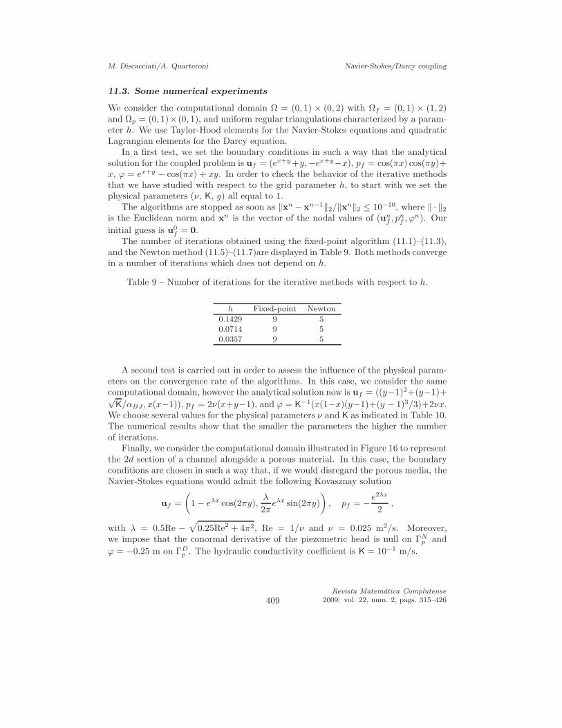
M. Discacciati/A. Quarteroni Navier-Stokes/Darcy coupling
11.3. Some numerical experiments
We consider the computational domain Ω = (0, 1) × (0, 2) with Ωf = (0, 1) × (1, 2)and Ωp = (0, 1)× (0, 1), and uniform regular triangulations characterized by a param-eter h. We use Taylor-Hood elements for the Navier-Stokes equations and quadraticLagrangian elements for the Darcy equation.
In a first test, we set the boundary conditions in such a way that the analyticalsolution for the coupled problem is uf = (ex+y+y,−ex+y−x), pf = cos(πx) cos(πy)+x, ϕ = ex+y − cos(πx) + xy. In order to check the behavior of the iterative methodsthat we have studied with respect to the grid parameter h, to start with we set thephysical parameters (ν, K, g) all equal to 1.
The algorithms are stopped as soon as ‖xn − xn−1‖2/‖xn‖2 ≤ 10−10, where ‖ · ‖2
is the Euclidean norm and xn is the vector of the nodal values of (unf , p
nf , ϕ
n). Our
initial guess is u0f = 0.
The number of iterations obtained using the fixed-point algorithm (11.1)–(11.3),and the Newton method (11.5)–(11.7)are displayed in Table 9. Both methods convergein a number of iterations which does not depend on h.
Table 9 – Number of iterations for the iterative methods with respect to h.
h Fixed-point Newton
0.1429 9 50.0714 9 50.0357 9 5
A second test is carried out in order to assess the influence of the physical param-eters on the convergence rate of the algorithms. In this case, we consider the samecomputational domain, however the analytical solution now is uf = ((y−1)2+(y−1)+√
K/αBJ , x(x−1)), pf = 2ν(x+y−1), and ϕ = K−1(x(1−x)(y−1)+(y − 1)3/3)+2νx.
We choose several values for the physical parameters ν and K as indicated in Table 10.The numerical results show that the smaller the parameters the higher the numberof iterations.
Finally, we consider the computational domain illustrated in Figure 16 to representthe 2d section of a channel alongside a porous material. In this case, the boundaryconditions are chosen in such a way that, if we would disregard the porous media, theNavier-Stokes equations would admit the following Kovasznay solution
uf =
(
1 − eλx cos(2πy),λ
2πeλx sin(2πy)
)
, pf = −e2λx
2,
with λ = 0.5Re −√
0.25Re2 + 4π2, Re = 1/ν and ν = 0.025 m2/s. Moreover,we impose that the conormal derivative of the piezometric head is null on ΓN
p and
ϕ = −0.25 m on ΓDp . The hydraulic conductivity coefficient is K = 10−1 m/s.
409Revista Matematica Complutense
2009: vol. 22, num. 2, pags. 315–426
M. Discacciati/A. Quarteroni Navier-Stokes/Darcy coupling
Table 10 – Convergence behavior of the iterative methods with respect to the param-eters ν and K.
Number of iterations for the fixed-point methodν K h = 0.1429 h = 0.0714 h = 0.0357
1 1 7 7 71 10−4 5 5 5
10−1 10−1 10 10 1010−2 10−1 15 15 1510−2 10−3 13 13 13
Number of iterations for the Newton methodν K h = 0.1429 h = 0.0714 h = 0.0357
1 1 4 4 41 10−4 4 4 4
10−1 10−1 5 5 510−2 10−1 6 6 610−2 10−3 6 6 6
We have solved this problem using two different grids and adopting the Newtonmethod. The convergence results are reported in Table 11, the computed velocity andpiezometric head are displayed in Figure 17.
Table 11 – Newton iterations to solve the problem illustrated in Figure 16.
Grid elements Newton iterations
792 73168 8
Concerning the computational costs, let us point out that the fixed-point algorithmrequires at each iteration the assembly of the matrix corresponding to the lineariza-tion of the Navier-Stokes equations and the solution of a linear system involving thevariables in both Ωf and Ωp. The Newton method is slightly more expensive sinceone has to assemble two matrices at each iteration and to update the right-hand side.The system to be solved features a similar structure to the one for fixed-point. Thesetwo methods are comparable since the additional cost required for assembling theNavier-Stokes system pays back with fewer iterations.
Remark 11.4. To solve (4.11)–(4.12), one could also consider the following precondi-tioned Richardson method : given u0
f ∈ Hf , ϕ0 ∈ Hp, for n ≥ 1, find unf ∈ Hf , qn
f ∈ Q,
Revista Matematica Complutense
2009: vol. 22, num. 2, pags. 315–426 410
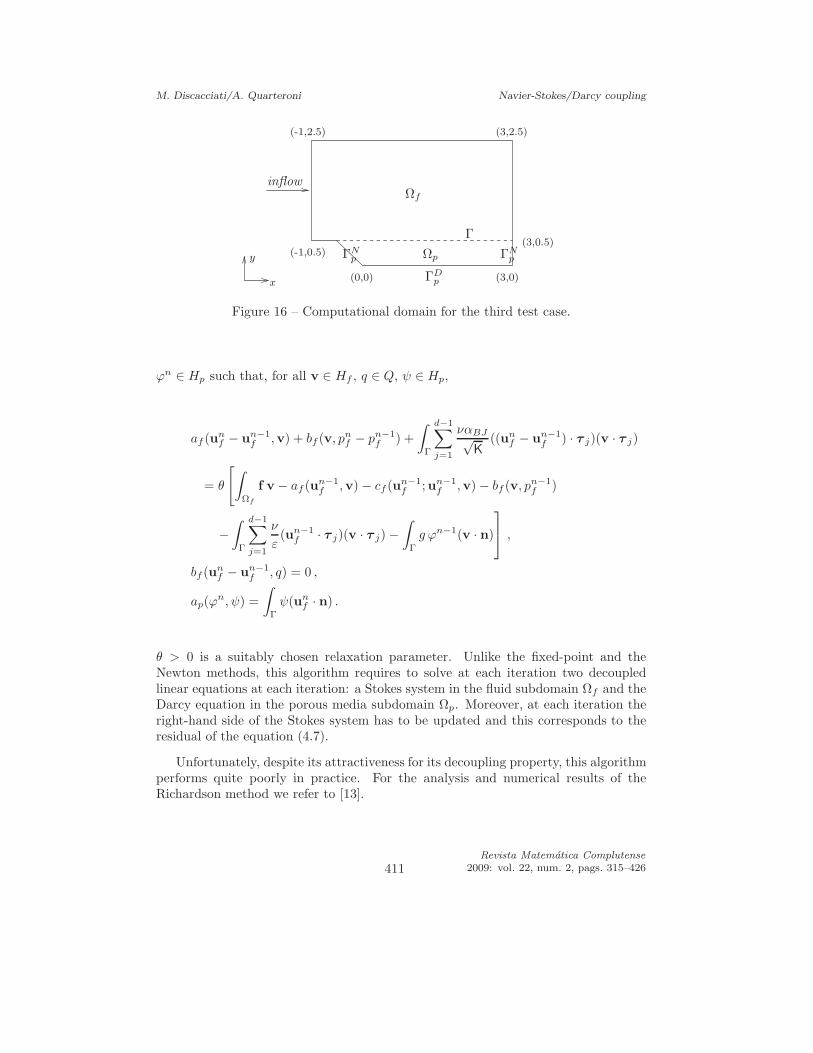
M. Discacciati/A. Quarteroni Navier-Stokes/Darcy coupling
Ωf
Ωp
Γ
ΓDp
ΓNpΓN
p
x
y
inflow
(-1,2.5) (3,2.5)
(-1,0.5)(3,0.5)
(0,0) (3,0)
Figure 16 – Computational domain for the third test case.
ϕn ∈ Hp such that, for all v ∈ Hf , q ∈ Q, ψ ∈ Hp,
af (unf − un−1
f ,v) + bf (v, pnf − pn−1
f ) +
∫
Γ
d−1∑
j=1
ναBJ√K
((unf − un−1
f ) · τ j)(v · τ j)
= θ
[
∫
Ωf
f v − af (un−1f ,v) − cf (un−1
f ;un−1f ,v) − bf (v, pn−1
f )
−∫
Γ
d−1∑
j=1
ν
ε(un−1
f · τ j)(v · τ j) −∫
Γ
g ϕn−1(v · n)
,
bf (unf − un−1
f , q) = 0 ,
ap(ϕn, ψ) =
∫
Γ
ψ(unf · n) .
θ > 0 is a suitably chosen relaxation parameter. Unlike the fixed-point and theNewton methods, this algorithm requires to solve at each iteration two decoupledlinear equations at each iteration: a Stokes system in the fluid subdomain Ωf and theDarcy equation in the porous media subdomain Ωp. Moreover, at each iteration theright-hand side of the Stokes system has to be updated and this corresponds to theresidual of the equation (4.7).
Unfortunately, despite its attractiveness for its decoupling property, this algorithmperforms quite poorly in practice. For the analysis and numerical results of theRichardson method we refer to [13].
411Revista Matematica Complutense
2009: vol. 22, num. 2, pags. 315–426
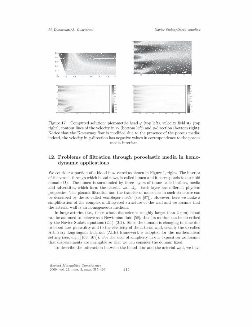
M. Discacciati/A. Quarteroni Navier-Stokes/Darcy coupling
0.5 0 0.5 1 1.5 2 2.5 30
0.1
0.2
0.3
0.4
0.5
1 0.5 0 0.5 1 1.5 2 2.5 30.5
1
1.5
2
2.5
1 0.5 0 0.5 1 1.5 2 2.5 30.5
1
1.5
2
2.5
0.4
0.3
0.2
0.1
0
0.1
0.2
0.3
0.4
0.5
0.6
1 0.5 0 0.5 1 1.5 2 2.5 30.5
1
1.5
2
2.5
1.5
1
0.5
0
0.5
1
1.5
2
2.5
3
3.5
Figure 17 – Computed solution: piezometric head ϕ (top left), velocity field uf (topright), contour lines of the velocity in x- (bottom left) and y-direction (bottom right).Notice that the Kovasznay flow is modified due to the presence of the porous media:indeed, the velocity in y-direction has negative values in correspondence to the porous
media interface.
12. Problems of filtration through poroelastic media in hemo-dynamic applications
We consider a portion of a blood flow vessel as shown in Figure 1, right. The interiorof the vessel, through which blood flows, is called lumen and it corresponds to our fluiddomain Ωf . The lumen is surrounded by three layers of tissue called intima, mediaand adventitia, which form the arterial wall Ωp. Each layer has different physicalproperties. The plasma filtration and the transfer of molecules in such structure canbe described by the so-called multilayer model (see [87]). However, here we make asimplification of the complex multilayered structure of the wall and we assume thatthe arterial wall is an homogeneous medium.
In large arteries (i.e., those whose diameter is roughly larger than 2 mm) bloodcan be assumed to behave as a Newtonian fluid [58], thus its motion can be describedby the Navier-Stokes equations (2.1)–(2.2). Since the domain is changing in time dueto blood flow pulsatility and to the elasticity of the arterial wall, usually the so-calledArbitrary Lagrangian Eulerian (ALE) framework is adopted for the mathematicalsetting (see, e.g., [103, 107]). For the sake of simplicity in our exposition we assumethat displacements are negligible so that we can consider the domain fixed.
To describe the interaction between the blood flow and the arterial wall, we have
Revista Matematica Complutense
2009: vol. 22, num. 2, pags. 315–426 412
M. Discacciati/A. Quarteroni Navier-Stokes/Darcy coupling
to consider a poroelastic model for the wall.A porous medium is defined as a mixture of a solid material, called skeleton or
matrix, and connecting pores filled with fluid. The fluid and the solid are assumed tobe incompressible. Consequently, the dynamics of such a medium can be describedby the Biot system [25, 26, 27]: ∀t > 0,
ρp∂tus + ρd∂tq−∇ · σEs (η) + ∇pp = fs in Ωp, (12.1)
ρd∂tus + ρd∂tq
n+K−1q + ∇pp = fd in Ωp, (12.2)
∇ · (us + q) = 0 in Ωp. (12.3)
The momentum equation for the balance of total forces is (12.1), while (12.2) is themomentum conservation equation for the fluid phase only, and (12.3) is the incom-pressibility constraint. ρd is the density of the fluid in the pores, ρp = ρs(1−n)+ρdnthe density of the saturated porous medium, ρs the density of the solid material, andn the porosity. The latter is the ratio of the pore volume over the total volume (pore+ skeleton) (see (2.3)).
We denote by us = ∂tη the velocity of the skeleton, where η is the displacement ofthe porous structure. q is the filtration velocity, i.e., the relative velocity of the fluidphase with respect to the solid one: q = n(up − us). Here, up is the velocity of thefluid in the porous medium, K is the hydraulic conductivity tensor (see (2.4)). Theeffective Cauchy stress tensor of the matrix is σE
s and it is related to the displacementof the porous structure η by a suitable constitutive law. For example, we can considerthe linear Saint-Venant Kirchhoff three-dimensional elastic model:
σEs (η) = 2µℓǫ(η) + λℓ(∇ · η)I,
where ǫ(η) = (∇η + ∇T η)/2, µℓ and λℓ are the Lame constants, representing theshear and dilation moduli of elasticity. The first constant accounts for distortion andthe second for compression of the medium [46].
The pressure of the fluid in the pore is given by pp. We define the total Cauchystress for the poroelastic structure as
σs = −ppI + σEs .
The right-hand side vectors fs and fd account for external body forces.Typical values of the physical parameters in hemodynamic applications are re-
ported in Table 12.
Notice that the Biot system (12.1)–(12.3) extends the Darcy equations takinginto account not only the filtration through the porous medium but also the elasticproperties of the porous medium itself.
In order for system (12.1)–(12.3) to be well-posed, proper initial and boundaryconditions must be imposed. In the following, the boundary conditions on ∂Ωp \Γ are
413Revista Matematica Complutense
2009: vol. 22, num. 2, pags. 315–426
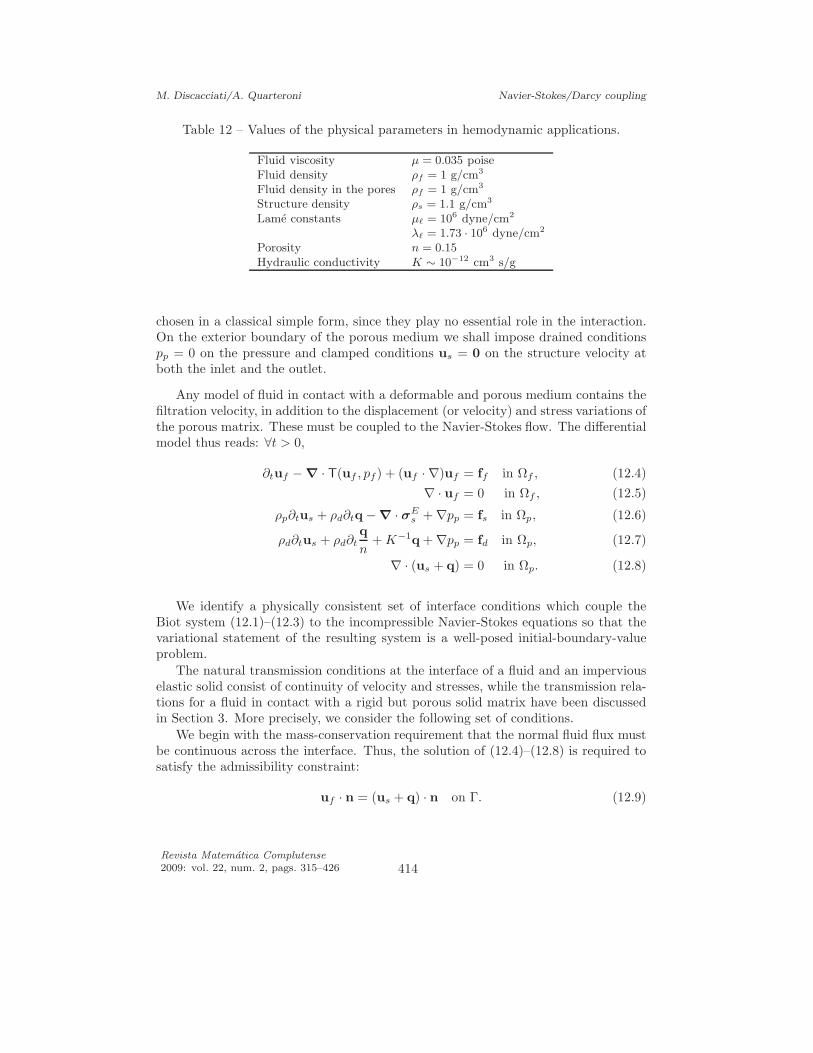
M. Discacciati/A. Quarteroni Navier-Stokes/Darcy coupling
Table 12 – Values of the physical parameters in hemodynamic applications.
Fluid viscosity µ = 0.035 poiseFluid density ρf = 1 g/cm3
Fluid density in the pores ρf = 1 g/cm3
Structure density ρs = 1.1 g/cm3
Lame constants µℓ = 106 dyne/cm2
λℓ = 1.73 · 106 dyne/cm2
Porosity n = 0.15Hydraulic conductivity K ∼ 10−12 cm3 s/g
chosen in a classical simple form, since they play no essential role in the interaction.On the exterior boundary of the porous medium we shall impose drained conditionspp = 0 on the pressure and clamped conditions us = 0 on the structure velocity atboth the inlet and the outlet.
Any model of fluid in contact with a deformable and porous medium contains thefiltration velocity, in addition to the displacement (or velocity) and stress variations ofthe porous matrix. These must be coupled to the Navier-Stokes flow. The differentialmodel thus reads: ∀t > 0,
∂tuf − ∇ · T(uf , pf) + (uf · ∇)uf = ff in Ωf , (12.4)
∇ · uf = 0 in Ωf , (12.5)
ρp∂tus + ρd∂tq − ∇ · σEs + ∇pp = fs in Ωp, (12.6)
ρd∂tus + ρd∂tq
n+K−1q + ∇pp = fd in Ωp, (12.7)
∇ · (us + q) = 0 in Ωp. (12.8)
We identify a physically consistent set of interface conditions which couple theBiot system (12.1)–(12.3) to the incompressible Navier-Stokes equations so that thevariational statement of the resulting system is a well-posed initial-boundary-valueproblem.
The natural transmission conditions at the interface of a fluid and an imperviouselastic solid consist of continuity of velocity and stresses, while the transmission rela-tions for a fluid in contact with a rigid but porous solid matrix have been discussedin Section 3. More precisely, we consider the following set of conditions.
We begin with the mass-conservation requirement that the normal fluid flux mustbe continuous across the interface. Thus, the solution of (12.4)–(12.8) is required tosatisfy the admissibility constraint:
uf · n = (us + q) · n on Γ. (12.9)
Revista Matematica Complutense
2009: vol. 22, num. 2, pags. 315–426 414
M. Discacciati/A. Quarteroni Navier-Stokes/Darcy coupling
For the balance of the normal stresses in the fluid phase across Γ, we have
−n · T(uf , pf ) · n = pp. (12.10)
The conservation of momentum requires that the total stress of the porous mediumis balanced by the total stress of the fluid:
σs · n = T(uf , pf ) · n. (12.11)
Finally, the fluid tangential stress (which is equal to the one of the solid phase) isassumed to be proportional to the slip rate according to the Beavers-Joseph-Saffmancondition:
τ j · T(uf , pf ) · n = −αBJ√K
(uf − us) · τ j , j = 1, . . . , d− 1. (12.12)
The global coupled system is then non-linear with a structure similar to the Navier-Stokes/Darcy system that we have analyzed in Section 6. Fixed-point of Newtonmethods can be used for the linearization of the Navier-Stokes/Biot coupled system.To solve the linear fluid-poroelastic-structure interaction problem, in [107, 18] severalmethods are proposed based both on the so-called monolytic approach and on domaindecomposition methods. In the first case the linear system obtained after time andspace discretizations is solved using direct or iterative methods with ad-hoc precondi-tioners (see [108, 17, 16]). On the other hand, partitioned procedures derived from adomain decomposition viewpoint feature similar structures to the Dirichlet-Neumannor Robin-Robin algorithms that we have illustrated in Section 8.4 and 10, respectively,for fluid-groundwater coupling. We refer to [107, 18] for an extensive analysis of thesemethods and for several numerical results.
Finally, let us point out that the finite element discretization of problem (12.4)–(12.12) can be carried out in analogous way to the Navier-Stokes/Darcy case usinginf-sup stable finite element spaces or any convenient stabilization techniques. Inparticular, in [107] an effective stabilization strategy based on variational multiscalemethods is investigated.
Appendix
A. Some existence and uniqueness results for non-linear prob-lems
In this section we recall some existence and uniqueness results for non-linear saddle-point problems, referring the reader to, e.g., [35, 36, 37, 42, 74] for a rigorous study.
Let (X, ‖ · ‖X) and (Y, ‖ · ‖Y ) be two real Hilbert spaces and consider a bilinearcontinuous form b(·, ·) : X×Y → R, (v, q) → b(v, q), and a trilinear form a(·; ·, ·) : X×
415Revista Matematica Complutense
2009: vol. 22, num. 2, pags. 315–426
M. Discacciati/A. Quarteroni Navier-Stokes/Darcy coupling
X ×X → R, (w, u, v) → a(w;u, v), where, for w ∈ X the mapping (u, v) → a(w;u, v)is a bilinear continuous form on X ×X .
Then, we consider the following problem: given l ∈ X ′, find a pair (u, p) ∈ X ×Ysatisfying
a(u;u, v) + b(v, p) = 〈l, v〉 ∀v ∈ Xb(u, q) = 0 ∀q ∈ Y.
(A.1)
Introducing the linear operators A(w) ∈ L(X ;X ′) for w ∈ X , and B ∈ L(X ;Y ′):
〈A(w)u, v〉 = a(w;u, v) ∀u, v ∈ X,
〈Bv, q〉 = b(v, q) ∀v ∈ X, ∀q ∈ Y,
problem (A.1) becomes:find (u, p) ∈ X × Y such that
A(u)u +BT p = l in X ′ ,Bu = 0 in Y ′ .
Taking V = Ker(B), we associate (A.1) with the problem:
find u ∈ V : a(u;u, v) = 〈l, v〉 ∀v ∈ V , (A.2)
or, equivalently:find u ∈ V such that ΠA(u)u = Π l in V ′, where the linear operator Π ∈ L(X ′;V ′)
is defined by 〈Π l, v〉 = 〈l, v〉, ∀v ∈ V .If (u, p) is a solution of problem (A.1), then u solves (A.2). The converse may
be proved provided an inf-sup condition holds. Indeed, the following results can beproved.
Theorem A.1 (Existence and uniqueness). Suppose that:
(i) The bilinear form a(w; ·, ·) is uniformly elliptic in the Hilbert space V with re-spect to w, i.e., there exists a constant α > 0 such that
a(w; v, v) ≥ α‖v‖2X ∀v, w ∈ V.
(ii) The mapping w → ΠA(w) is locally Lipschitz-continuous in V , i.e., there existsa continuous and monotonically increasing function L : R
+ → R+ such that for
all m > 0
|a(w1;u, v) − a(w2;u, v)| ≤ L(m)‖u‖X‖v‖X‖w1 − w2‖X
∀u, v ∈ V , ∀w1, w2 ∈ Sm with Sm = w ∈ V : ‖w‖X ≤ m.(iii) It holds that
‖Π l‖V ′
α2L
(‖Π l‖V ′
α
)
< 1 .
Revista Matematica Complutense
2009: vol. 22, num. 2, pags. 315–426 416

M. Discacciati/A. Quarteroni Navier-Stokes/Darcy coupling
Then (A.2) has a unique solution u ∈ V .
We consider now problem (A.1).
Theorem A.2. Assume that the bilinear form b(·, ·) satisfies the inf-sup condition:there exists a positive constant β > 0, such that
∀q ∈ Y, ∃v ∈ X, v 6= 0 : b(v, q) ≥ β‖v‖X‖q‖Y .
Then for each solution u of (A.2) there exists a unique p ∈ Y such that the pair (u, p)is a solution of (A.1).
Finally, let us recall an important result on the convergence of Newton methodsin Banach spaces.
Let X and Y be two Banach spaces. We consider the sphere of radius R > 0centered in x0 ∈ X : Ω = x ∈ X : ||x − x0||X < R, and the closed sphere of radius0 < r < R centered in x0: Ω0 = x ∈ X : ||x − x0||X ≤ r. We assume that Ωcontains a zero of an operator P : Ω ⊂ X → Y , i.e., a point x∗ ∈ Ω such thatP(x∗) = 0.
If P has a continuous Gateaux derivative in Ω, we can apply the Newton methodto compute the zero x∗: given an initial approximation x0 ∈ Ω of x∗, for n ≥ 0,
xn+1 = xn − [P ′(xn)]−1(P(xn)) ,
assuming that [P ′(xn)]−1 exists.
Alternatively, we can use the modified Newton algorithm: given x0 ∈ Ω, for n ≥ 0,
xn+1 = xn − [P ′(x0)]−1(P(xn)) .
Concerning the convergence of these methods, we have the following theorem (see [86,Theorem 6 (1.XVIII), page 708]).
Theorem A.3 (Kantorovich Theorem). Let P be defined on Ω ⊂ X with continuoussecond derivative in Ω0. Moreover assume that:
(1) There exists the continuous linear operator [P ′(x0)]−1.
(2) There exists a positive constant K1 > 0 : ||[P ′(x0)]−1(P(x0))||X ≤ K1.
(3) There exists a positive constant K2 > 0 : ||[P ′(x0)]−1P ′′(x)||X ≤ K2 for allx ∈ Ω0.
If
K3 = K1K2 ≤ 1
2, (A.3)
417Revista Matematica Complutense
2009: vol. 22, num. 2, pags. 315–426
M. Discacciati/A. Quarteroni Navier-Stokes/Darcy coupling
and the radius r of Ω0 satisfies
r ≥ r0 =1 −
√1 − 2K3
K3K1 , (A.4)
then, there exists a zero x∗ of P to which the Newton and the modified Newton methodsconverge. In this case,
||x∗ − x0||X ≤ r0. (A.5)
Furthermore, if for K3 < 1/2
r < r1 =1 +
√1 − 2K3
K3K1 , (A.6)
or for K3 = 1/2r ≤ r1 , (A.7)
the solution x∗ is unique in the sphere Ω0.The convergence rate of the Newton method is characterized by
||x∗ − xn||X ≤ 1
2n(2K3)
2n K1
K3, n ≥ 0, (A.8)
while that of the modified method, for K3 < 1/2, by
||x∗ − xn||X ≤ K1
K3(1 −
√
1 − 2K3)n+1 , n ≥ 0. (A.9)
Acknowledgement. The authors would like to acknowledge the anonymous refereefor many useful comments and suggestions that have led to improving the originalmanuscript.
References
[1] J. Aarnes. Efficient domain decomposition methods for elliptic problems arising fromflows in heterogeneous porous media. Comput. Vis. Sci., 8(2):93–106, 2005.
[2] J. Aarnes and Y. Efendiev. An adaptive multiscale method for simulation of fluid flowin heterogeneous porous media. Multiscale Model. Simul., 5(3):918–939 (electronic),2006.
[3] J. Aarnes and B.-O. Heimsund. Multiscale discontinuous Galerkin methods for ellipticproblems with multiple scales. In Multiscale Methods in Science and Engineering,volume 44 of Lect. Notes Comput. Sci. Eng., pages 1–20. Springer, Berlin, 2005.
[4] J. Aarnes and T.Y. Hou. Multiscale domain decomposition methods for elliptic prob-lems with high aspect ratios. Acta Math. Appl. Sin. Engl. Ser., 18(1):63–76, 2002.
Revista Matematica Complutense
2009: vol. 22, num. 2, pags. 315–426 418
M. Discacciati/A. Quarteroni Navier-Stokes/Darcy coupling
[5] J.E. Aarnes. On the use of a mixed multiscale finite element method for greaterflexibility and increased speed or improved accuracy in reservoir simulation. MultiscaleModel. Simul., 2(3):421–439 (electronic), 2004.
[6] R.A. Adams. Sobolev Spaces. Academic Press, New York, 1975.
[7] V.I. Agoshkov. Poincare-Steklov operators and domain decomposition in finite dimen-sional spaces. In First International Symposium on Domain Decomposition Methodsfor Partial Differential Equations, Paris 1987, pages 73–112. SIAM, Philadephia, 1988.
[8] V.I. Agoshkov and V.I. Lebedev. Variational algorithms of the domain decompositionmethod. Sov. J. Numer. Anal. Math. Modelling, 5(1):27–46, 1990. Originally publishedin Russian as Preprint No. 54, Dept. Numer. Math. URSS Acad. Sci. Moscow, 1983.
[9] R.E. Alcouffe, A. Brandt, J.E. Dendy, and J.W. Painter. The multigrid method forthe diffusion equation with strongly discontinuous coefficients. SIAM J. Sci. Statist.Comput., 2(4):430–454, 1981.
[10] T. Arbogast, J. Douglas, and U. Hornung. Derivation of the double porosity modelof single phase flow via homogenization theory. SIAM J. Math. Anal., 21(4):430–454,1990.
[11] D.N. Arnold, F. Brezzi, B. Cockburn, and L.D. Marini. Unified analysis of discontinu-ous Galerkin methods for elliptic problems. SIAM J. Numer. Anal., 39(5):1749–1779,2002.
[12] I. Babuska and J.E. Osborn. Generalized finite element methods: their performanceand their relation to mixed methods. SIAM J. Numer. Anal., 20(3):510–536, 1983.
[13] L. Badea, M. Discacciati, and A. Quarteroni. Numerical analysis of the Navier-Stokes/Darcy coupling. Technical report, Ecole Polytechnique Federale de Lausanne,IACS-CMCS, 2008.
[14] S. Badia and R. Codina. Unified stabilized finite element formulations for the Stokesand the Darcy problems. Technical report, Universitat Politecnica de Catalunya, 2008.
[15] S. Badia, F. Nobile, and C. Vergara. Robin-Robin preconditioned Krylov methods forfluid-structure interaction problems. Technical Report 19/2008, MOX - Politecnico diMilano, 2008.
[16] S. Badia, A. Quaini, and A. Quarteroni. Modular vs. non-modular preconditioners forfluid-structure systems with large added-mass effect. Comput. Methods Appl. Mech.Engrg., 197(49–50):4216–4232, 2008.
[17] S. Badia, A. Quaini, and A. Quarteroni. Splitting methods based on algebraic factor-ization for fluid-structure interaction. SIAM J. Sci. Comput., 30(4):1778–1805, 2008.
[18] S. Badia, A. Quaini, and A. Quarteroni. Coupling Biot and Navier-Stokes problemsfor fluid-poroelastic structure interaction. Technical report, Universitat Politcnica deCatalunya, 2009. Available at http://hdl.handle.net/2072/13533.
[19] P. Bastian. Higher order discontinuous Galerkin methods for flow and transport inporous media. In E. Baensch, editor, Challenges in Scientific Computing CISC2002.Lecture Notes in Computational Science and Engineering (35), pages 1–22. Springer,Berlin and Heidelberg, 2003.
419Revista Matematica Complutense
2009: vol. 22, num. 2, pags. 315–426
M. Discacciati/A. Quarteroni Navier-Stokes/Darcy coupling
[20] J. Bear. Hydraulics of Groundwater. McGraw-Hill, New York, 1979.
[21] G.S. Beavers and D.D. Joseph. Boundary conditions at a naturally permeable wall. J.Fluid Mech., 30:197–207, 1967.
[22] C. Bernardi, Y. Maday, and F. Rapetti. Discretisations variationnelles de problemesaux limites elliptiques, volume 45 of Mathematiques & Applications (Berlin) [Mathe-matics & Applications]. Springer-Verlag, Berlin, 2004.
[23] C. Bernardi, T.C. Rebollo, F. Hecht, and Z. Mghazli. Mortar finite element discretiza-tion of a model coupling Darcy and Stokes equations. M2AN Math. Model. Numer.Anal., 42(3):375–410, 2008.
[24] H. Berninger. Domain Decomposition Methods for Elliptic Problems with JumpingNonlinearities and Application to the Richards Equation. PhD thesis, Freie UniversitatBerlin, 2007.
[25] M.A. Biot. General theory of three-dimensional consolidation. J. Appl. Phys., 12:155–164, 1941.
[26] M.A. Biot. Theory of elasticity and consolidation for a porous anisotropic solid. J.Appl. Phys., 25:182–185, 1955.
[27] M.A. Biot. Theory of finite deformation of porous solids. Indiana Univ. Math. J.,21:597–620, 1971/72.
[28] A. Brandt. Multi-level adaptive solutions to boundary-value problems. Math. Comp.,31(138):333–390, 1977.
[29] F. Brezzi. On the existence, uniqueness and approximation of saddle-point prob-lems arising from Lagrange multipliers. Rev. Francaise Automat. Informat. RechercheOperationnelle, ser. Rouge, 8:129–151, 1974.
[30] F. Brezzi, J. Douglas Jr., R. Duran, and M. Fortin. Mixed finite elements for secondorder elliptic problems in three variables. Numer. Math., 51(2):237–250, 1987.
[31] F. Brezzi, J. Douglas Jr., M. Fortin, and L.D. Marini. Efficient rectangular mixedfinite elements in two and three space variables. RAIRO Model. Math. Anal. Numer.,21(4):581–604, 1987.
[32] F. Brezzi, J. Douglas Jr., and L.D. Marini. Two families of mixed finite elements forsecond order elliptic problems. Numer. Math., 47(2):217–235, 1985.
[33] F. Brezzi and M. Fortin. Mixed and Hybrid Finite Element Method. Springer, NewYork, 1991.
[34] F. Brezzi, L.P. Franca, T.J.R. Hughes, and A. Russo. b =∫
g. Comput. Methods Appl.Mech. Engrg., 145((3–4)):329–339, 1997.
[35] F. Brezzi, J. Rappaz, and P.A. Raviart. Finite dimensional approximation of nonlinearproblems. Part I: Branches of nonlinear solutions. Numer. Math., 36:1–25, 1980.
[36] F. Brezzi, J. Rappaz, and P.A. Raviart. Finite dimensional approximation of nonlinearproblems. Part II: Limit points. Numer. Math., 37:1–28, 1981.
[37] F. Brezzi, J. Rappaz, and P.A. Raviart. Finite dimensional approximation of nonlinearproblems. Part III: Simple bifurcation points. Numer. Math., 38:1–30, 1981.
Revista Matematica Complutense
2009: vol. 22, num. 2, pags. 315–426 420
M. Discacciati/A. Quarteroni Navier-Stokes/Darcy coupling
[38] H.C. Brinkman. A calculation of the viscous force exerted by a flowing fluid on a denseswarm of particles. Appl. Sci. Res. A, 1:27–34, 1947.
[39] E. Burman. Pressure projection stabilizations for galerkin approximations of Stokes’and Darcy’s problems. Numer. Methods Partial Differential Equations, 24(1):127–143,2008.
[40] E. Burman and P. Hansbo. A unified stabilized method for Stokes’ and Darcy’s equa-tions. J. Comput. Appl. Math., 198(1):35–51, 2007.
[41] E. Burman and P. Zunino. A domain decomposition method based on weighted in-terior penalties for advection-diffusion-reaction problems. SIAM J. Numer. Anal.,44(4):1612–1638, 2006.
[42] G. Caloz and J. Rappaz. Numerical Analysis for Nonlinear and Bifurcation Problems.In Handbook of Numerical Analysis, Vol. V, pages 487–637. North-Holland, Amster-dam, 1997.
[43] Y. Cao, M. Gunzburger, F. Hua, and X. Wang. Coupled Stokes-Darcy model withBeavers-Joseph interface boundary conditions. Comm. Math. Sci., 2008. To appear.
[44] Z. Chen and T.Y. Hou. A mixed finite element method for elliptic problems withrapidly oscillating coefficients. Math. Comput., 72:541–576, 2002.
[45] P.G. Ciarlet. The Finite Element Method for Elliptic Problems. North-Holland Pub-lishing Co., Amsterdam, 1978.
[46] P.G. Ciarlet. Mathematical elasticity. Vol. I, volume 20 of Studies in Mathematics andits Applications. North-Holland Publishing Co., Amsterdam, 1988. Three-dimensionalelasticity.
[47] B. Cockburn, G. E. Karniadakis, and C.-W. Shu. The development of discontinuousGalerkin methods. In Discontinuous Galerkin methods (Newport, RI, 1999), volume 11of Lect. Notes Comput. Sci. Eng., pages 3–50. Springer, Berlin, 2000.
[48] R. Codina. Stabilized finite element approximation of transient incompressible flowsusing orthogonal subscales. Comput. Methods Appl. Mech. Engrg., 191:4295–4321,2002.
[49] C. D’Angelo and P. Zunino. A finite element method based on weighted interiorpenalties for heterogenenous incompressible flows. Technical Report 14/2008, MOX -Politecnico di Milano, 2008.
[50] H. Darcy. Les Fontaines Publiques de la Ville de Dijon. Dalmont, Paris, 1856.
[51] R. Dautray and J.-L. Lions. Mathematical Analysis and Numerical Methods for Scienceand Technology, volume 2. Springer, Berlin, 1988.
[52] S. Deparis, M. Discacciati, and A. Quarteroni. A domain decomposition frameworkfor fluid-structure interaction problems. In C. Groth and D.W. Zingg, editors, Com-putational Fluid Dynamics 2004, pages 41–58. Springer, New York, 2006.
[53] M. Discacciati. Domain Decomposition Methods for the Coupling of Surface andGroundwater Flows. PhD thesis, Ecole Polytechnique Federale de Lausanne, Switzer-land, 2004.
[54] M. Discacciati. An operator-splitting approach to nonoverlapping domain decomposi-tion methods. Technical Report 14, Section de Mathematiques, EPFL, 2004.
421Revista Matematica Complutense
2009: vol. 22, num. 2, pags. 315–426
M. Discacciati/A. Quarteroni Navier-Stokes/Darcy coupling
[55] M. Discacciati, E. Miglio, and A. Quarteroni. Mathematical and numerical models forcoupling surface and groundwater flows. Appl. Numer. Math., 43:57–74, 2002.
[56] M. Discacciati and A. Quarteroni. Analysis of a domain decomposition method forthe coupling of Stokes and Darcy equations. In F. Brezzi, A. Buffa, S. Corsaro, andA. Murli, editors, Numerical Mathematics and Advanced Applications, ENUMATH2001, pages 3–20. Springer. Milan, 2003.
[57] M. Discacciati, A. Quarteroni, and A. Valli. Robin-Robin domain decomposition meth-ods for the Stokes-Darcy coupling. SIAM J. Numer. Anal., 45(3):1246–1268 (elec-tronic), 2007.
[58] D.A. Mc Donald. Blood Flow in Arteries. Edward Arnoldt Ltd., London, 1990.
[59] M. Dorobantu and B. Engquist. Wavelet-based numerical homogenization. SIAM J.Numer. Anal., 35:540–559, 1998.
[60] M. Dryja, M.V. Sarkis, and O.B. Widlund. Multilevel Schwarz methods for el-liptic problems with discontinuous coefficients in three dimensions. Numer. Math.,72(3):313–348, 1996.
[61] L.J. Durlofsky. Coarse scale models of two phase flow in heterogeneous reservoirs:volume avaraged equations and their relationship to existing upscaling techniques.Comput. Geosci., 2(2):73–92, 1998.
[62] W. E and B. Engquist. The heterogeneous multiscale method. Commun. Math. Sci.,1(1):87–132, 2003.
[63] W. E and B. Engquist. Multiscale modeling and computation. Notices Amer. Math.Soc., 50(9):1062–1070, 2003.
[64] W. E and B. Engquist. The heterogeneous multi-scale method for homogenizationproblems. In Multiscale Methods in Science and Engineering, volume 43 of Lect. NotesComput. Sci. Eng., pages 89–110. Springer, Berlin, 2005.
[65] Y.R. Efendiev, T.Y. Hou, and X.-H. Wu. Convergence of a nonconforming multiscalefinite element method. SIAM J. Numer. Anal., 37(3):888–910, 2000.
[66] H.I. Ene and E. Sanchez-Palencia. Equations et phenomenes de surface pourl’ecoulement dans un modele de milieu poreux. J. Mecanique, 14(1):73–108, 1975.
[67] P. Forchheimer. Wasserbewegung durch Boden. Z. Ver. Deutsch. Ing., 45:1782–1788,1901.
[68] J. Galvis and M. Sarkis. BDD and FETI methods for mortar coupling of Stokes-Darcy.Technical Report Serie A 563, Instituto de Matematica Pura e Aplicada, Brazil, 2007.Submitted.
[69] J. Galvis and M. Sarkis. Non-matching mortar discretization analysis for the couplingStokes-Darcy equations. Electon. Trans. Numer. Anal., 26:350–384, 2007.
[70] J.C. Galvis and M. Sarkis. Inf-sup for coupling Stokes-Darcy. In A. Loula et al.,editor, XXV Iberian Latin American Congress in Computational Methods in Engi-neering, 2005, Recife. Proceedings of the XXV Iberian Latin American Congress inComputational Methods in Engineering, Recife, Brazil, 2004. Universidade Federal dePernambuco, 2004.
Revista Matematica Complutense
2009: vol. 22, num. 2, pags. 315–426 422
M. Discacciati/A. Quarteroni Navier-Stokes/Darcy coupling
[71] J.C. Galvis and M. Sarkis. Balancing domain decomposition methods for mortarcoupling Stokes-Darcy systems. In D.E. Keyes and O.B. Widlund, editors, DomainDecomposition Methods in Science and Engineering XVI, pages 373–380. Springer,Berlin and Heidelberg, 2006.
[72] G.N. Gatica, R. Oyarzua, and F.-J. Sayas. Convergence of a family of Galerkin dis-cretizations for the Stokes-Darcy coupled problem. Technical Report 08-11, Departa-mento de Ingegnerıa Matematica, Universidad de Conception, 2008.
[73] T. Giorgi. Derivation of the Forchheimer law via matched asymptotic expansions.Transport in Porous Media, 29:191–206, 1997.
[74] V. Girault and P.A. Raviart. Finite Element Methods for Navier-Stokes Equations.Theory and Algorithms. Springer, Berlin, 1986.
[75] V. Girault and B. Riviere. DG approximation of coupled Navier-Stokes and Darcyequations by Beaver-Joseph-Saffman interface condition. Technical Report TR-MATH07-09, University of Pittsburgh, Department of Mathematics, 2007.
[76] J.S. Hesthaven and T. Warburton. Nodal Discontinuous Galerkin Methods, volume 54of Texts in Applied Mathematics. Springer, New York, 2008. Algorithms, analysis, andapplications.
[77] H. Hoteit, J. Erhel, R. Mose, B. Philippe, and Ph. Ackerer. Numerical reliabilityfor mixed methods applied to flow problems in porous media. Comput. Geosciences,6:161–194, 2002.
[78] T.Y. Hou and X. Wu. A multiscale finite element method for elliptic problems incomposite materials and porous media. J. Comput. Phys., 134(1):169–189, 1997.
[79] T.Y. Hou, X. Wu, and Z. Cai. Convergence of a multiscale finite element method forelliptic problems with rapidly oscillating coefficients. Math. Comp., 68(227):913–943,1999.
[80] T.J.R. Hughes. Multiscale phenomena: Green’s functions, the Dirichlet-to-Neumannformulation, subgrid scale models, bubbles and the origins of stabilized methods. Com-put. Methods Appl. Mech. Engrg., 127:387–401, 1995.
[81] T.J.R. Hughes, G.R. Feijoo, L. Mazzei, and J.-B. Quincy. The variational multiscalemethod – a paradigm for computational mechanics. Comput. Methods Appl. Mech.Engrg., 166(1–2):3–24, 1998.
[82] O. Iliev, A. Mikelic, and P. Popov. On upscaling certain flows in deformable porousmedia. Multiscale Model. Simul., 7(1):93–123, 2008.
[83] W. Jager and A. Mikelic. On the boundary conditions at the contact interface betweena porous medium and a free fluid. Ann. Scuola Norm. Sup. Pisa Cl. Sci., 23:403–465,1996.
[84] W. Jager and A. Mikelic. On the interface boundary condition of Beavers, Joseph andSaffman. SIAM J. Appl. Math., 60(4):1111–1127, 2000.
[85] W. Jager, A. Mikelic, and N. Neuss. Asymptotic analysis of the laminar viscous flowover a porous bed. SIAM J. Sci. Comput., 22(6):2006–2028, 2001.
423Revista Matematica Complutense
2009: vol. 22, num. 2, pags. 315–426
M. Discacciati/A. Quarteroni Navier-Stokes/Darcy coupling
[86] L.V. Kantorovich and G.P. Akilov. Functional Analysis in Normed Spaces. Translatedfrom the Russian by D. E. Brown. Edited by A. P. Robertson. International Seriesof Monographs in Pure and Applied Mathematics, Vol. 46. The Macmillan Co., NewYork, 1964.
[87] G. Karner and K. Perktold. Effect of endothelial injury and increased blood pressure onalbumin accumulation in the arterial wall: a numerical study. J. Biomech., 33:709–715,2000.
[88] W.L. Layton, F. Schieweck, and I. Yotov. Coupling fluid flow with porous media flow.SIAM J. Num. Anal., 40:2195–2218, 2003.
[89] T. Levy and E. Sanchez-Palencia. On the boundary conditions for fluid flow in porousmedia. Int. J. Engng. Sci., 13:923–940, 1975.
[90] J.L. Lions and E. Magenes. Problemes aux Limites Non Homogenes et Applications,volume 1. Dunod, Paris, 1968.
[91] P.L. Lions. On the Schwarz alternating method III: a variant for non-overlappingsubdomains. In T.F. Chan et al., editor, Third International Symposium on Do-main Decomposition Methods for Partial Differential Equations, pages 202–231. SIAM,Philadelphia, 1990.
[92] A.F.D. Loula, F.A. Rochinha, and M.A. Murad. High-order gradient post-processingsfor second-order elliptic problems. Comput. Meth. Appl. Mech. Engrg., 128:361–381,1995.
[93] Y. Maday and F. Magoules. Optimized Schwarz methods without overlap for highlyheterogeneous media. Comput. Methods Appl. Mech. Engrg., 196(8):1541–1553, 2007.
[94] L.D. Marini and A. Quarteroni. A relaxation procedure for domain decompositionmethods using finite elements. Numer. Math., 55:575–598, 1989.
[95] E. Marusic-Paloka and A. Mikelic. The derivation of a nonlinear filtration law includingthe inertia effects via homogenization. Nonlin. Anal., 42:97–137, 2000.
[96] A. Masud and T.J.R. Hughes. A stabilized mixed finite element method for Darcyflow. Comput. Meth. Appl. Mech. Engrg., 191:4341–4370, 2002.
[97] E. Miglio. Mathematical and Numerical Modeling for Enviromental Applications. PhDthesis, Universita degli Studi di Milano, Politecnico di Milano, 2000.
[98] E. Miglio, A. Quarteroni, and F. Saleri. Coupling of free surface and groundwaterflows. Comput. Fluids, 32(1):73–83, 2003.
[99] J. Necas. Les Methodes Directes en Theorie des Equations Elliptiques. Masson, Paris,1967.
[100] J.-C. Nedelec. Mixed finite elements in R3. Numer. Math., 35:119–136, 1980.
[101] J.-C. Nedelec. A new family of mixed finite elements in R3. Numer. Math., 50(1):57–81,
1986.
[102] N. Neuss, W. Jager, and G. Wittum. Homogenization and multigrid. Computing,66(1):1–26, 2001.
[103] F. Nobile. Numerical Approximation of Fluid-Structure Interaction Problems with Ap-plications to Haemodynamics. PhD thesis, Ecole Polytechnique Federale de Lausanne,Switzerland, 2001.
Revista Matematica Complutense
2009: vol. 22, num. 2, pags. 315–426 424
M. Discacciati/A. Quarteroni Navier-Stokes/Darcy coupling
[104] J.T. Oden and K.S Vemaganti. Estimation of local modeling error and goal-orientedadaptive modeling of heterogeneous materials. I. Error estimates and adaptive algo-rithms. J. Comput. Phys., 164(1):22–47, 2000.
[105] L.E. Payne and B. Straughan. Analysis of the boundary condition at the interfacebetween a viscous fluid and a porous medium and related modelling questions. J.Math. Pures Appl., 77:317–354, 1998.
[106] D. Peaceman and H. Rachford. The numerical solution of parabolic and elliptic differ-ential equations. J. SIAM, 3:28–41, 1955.
[107] A. Quaini. Algorithms for Fluid-Structure Interaction Problems Arising in Hemody-namics. PhD thesis, Ecole Polytechnique Federale de Lausanne, Switzerland, 2008.Submitted.
[108] A. Quaini and A. Quarteroni. A semi-implicit approach for fluid-structure interac-tion based on an algebraic fractional step method. Math. Models Methods Appl. Sci.,17(6):957–983, 2007.
[109] A. Quarteroni and A. Valli. Numerical Approximation of Partial Differential Equa-tions. Springer, Berlin, 1994.
[110] A. Quarteroni and A. Valli. Domain Decomposition Methods for Partial DifferentialEquations. Oxford University Press, New York, 1999.
[111] P.-A. Raviart and J. M. Thomas. A mixed finite element method for 2nd order ellipticproblems. In Mathematical Aspects of Finite Element Methods (Proc. Conf., ConsiglioNaz. delle Ricerche (C.N.R.), Rome, 1975), pages 292–315. Lecture Notes in Math.,Vol. 606. Springer, Berlin, 1977.
[112] B. Riviere. Analysis of a discontinuous finite element method for the coupled Stokesand Darcy problems. J. Sci. Comput., 22(1):479–500, 2005.
[113] B. Riviere and I. Yotov. Locally conservative coupling of Stokes and Darcy flows.SIAM J. Numer. Anal., 42(5):1959–1977, 2005.
[114] Y. Saad. Iterative Methods for Sparse Linear Systems. Society for Industrial andApplied Mathematics, Philadelphia, second edition, 2003.
[115] P.G. Saffman. On the boundary condition at the interface of a porous medium. Stud.Appl. Math., 1:93–101, 1971.
[116] G. Sangalli. Capturing small scales in elliptic problems using a residual-free bubblesfinite element method. Multiscale Model. Simul., 1(3):485–503, 2003.
[117] L. Tartar. Incompressible fluid flow in a porous medium: convergence of the homog-enization process. In E. Sanchez-Palencia: Non-Homogeneous Media and VibrationTheory. Lecture Notes in Physics 127, pages 368–377. Springer, Berlin, 1980.
[118] J.M. Thomas. Sur l’Analyse Numerique des Methodes d’Elements Finis Hybrides etMixtes. PhD thesis, Universite Pierre et Marie Curie, 1977.
[119] A. Toselli and O. Widlund. Domain Decomposition Methods - Algorithms and Theory.Springer, New York, 2005.
[120] U. Hornung, editor. Homogenization and Porous Media, volume 6 of InterdisciplinaryApplied Mathematics. Springer, New York, 1997.
425Revista Matematica Complutense
2009: vol. 22, num. 2, pags. 315–426
M. Discacciati/A. Quarteroni Navier-Stokes/Darcy coupling
[121] B.I. Wohlmuth. Discretization Methods and Iterative Solvers Based on Domain De-composition, volume 17 of Lecture Notes in Computational Science and Engineering.Springer-Verlag, Berlin, 2001.
[122] X.H. Wu, Y. Efendiev, and T.Y. Hou. Analysis of upscaling absolute permeability.Discrete Contin. Dyn. Syst. Ser. B, 2(2):185–204, 2002.
[123] K. Yosida. Functional Analysis. Springer, Berlin, 1974.
[124] P. Zunino. Mathematical and Numerical Modeling of Mass Transfer in the VascularSystem. PhD thesis, Ecole Polytechnique Federale de Lausanne, Switzerland, 2002.
[125] P. Zunino. Mortar and discontinuous Galerkin methods based on weighted interiorpenalties. In U. Langer et al., editor, Domain Decomposition Methods in Science andEngineering XVII, volume 60 of Lect. Notes Comput. Sci. Eng., pages 321–327, Berlin,2008. Springer.
Revista Matematica Complutense
2009: vol. 22, num. 2, pags. 315–426 426