842 J. AIRCRAFT VOL. 25, NO. 9

Navier-Stokes Simulationfor Flow Past an Open Cavity

Deepak Om*The Boeing Company, Seattle, Washington

A two-dimensional Navier-Stokes code was developed to simulate the flow past an open cavity. The codeemploys the split explicit predictor-corrector algorithm of MacCormack in conservation law form. The purposewas to examine the unsteadiness of the shear layer and obtain details of the flowfield. Cavity flow was simulatedfor two different cavity sizes as well as for two different ramp shapes. Comparison with a wind-tunnelexperiment shows good agreement. Those flows that were observed to be steady in the experiment were alsosteady in the computation; those flows that exhibited unsteady behavior of the shear layer in the experiment werealso unsteady in the computation. Computations also showed that the shear-layer stability depends very stronglyon the shape of the aft ramp and, with a proper ramp shape, the effect of cavity size was negligible on theshear-layer stability. These conclusions, also in agreement with the experimental results, were very useful indesigning the cavity shape for the Boeing 767-AOA airplane.

Introduction

T HERE have been numerous experimental investigationsof flows over open cavities. Rossiter1 measured time-

averaged and unsteady pressures for a series of rectangularcavities. He found that the unsteady pressures contained bothrandom and periodic components. Spee2 conducted wind-tun-nel experiments on the unsteady flow over a cavity system athigh subsonic speeds to understand the interaction betweensound waves and two-dimensional transonic flows. Heller andBliss3 used a water table to simulate supersonic flow over openrectangular cavities and to explain the unsteady behavior ofthe shear layer. Franke and Carr4 studied the effects ofgeometric modifications for reducing flow-induced pressureoscillations in shallow, open, two-dimensional, rectangularcavities. Ethembabaoglu5 also examined various types ofgeometric modifications to reduce the amplitude of cavityoscillations. Rockwell and Naudascher6'7 have presented adetailed review of self-sustaining oscillations of the flow pastcavities.

Thus, extensive measurements exist to give a qualitativedescription of cavity-flow phenomena. However, numericalsimulations of cavity flow have not received the same kind ofattention. Borland8 used Euler equations to predict theunsteady flow over a rectangular cavity. Hankey and Shang9

obtained numerical solutions of the Navier-Stokes equationsfor an open cavity at supersonic speed.

The purpose of the present investigation was to conduct anumerical study of the cavity-flow phenomenon on a modifiedBoeing 767. The Boeing 767-AOA (Airborne Optical Adjunct)airplane currently in design includes a large cupola fairing ontop of the fuselage to house two optical sensor devices. Eachoptical sensor resides in its own compartment, one forwardand one aft. Each compartment has a viewing port on the sideof cupola, which will be opened during the observation part ofthe mission (Fig. 1). Therefore, the external cupola air mustflow past two large open cavities.

The intent here is to design a cavity configuration thatwould have acceptable aerodynamic, acoustic, and opticaltransmission characteristics. The thin, stable shear layer,

Presented as Paper 86-2628 at the AIAA Aircraft Systems, Designand Technology Meeting, Dayton, OH, Oct. 20-22, 1986; receivedSept. 30, 1987; revision received April 26, 1988. Copyright ©American Institute of Aeronautics and Astronautics, Inc., 1986. Allrights reserved.

*Senior Specialist Engineer. Member AIAA.

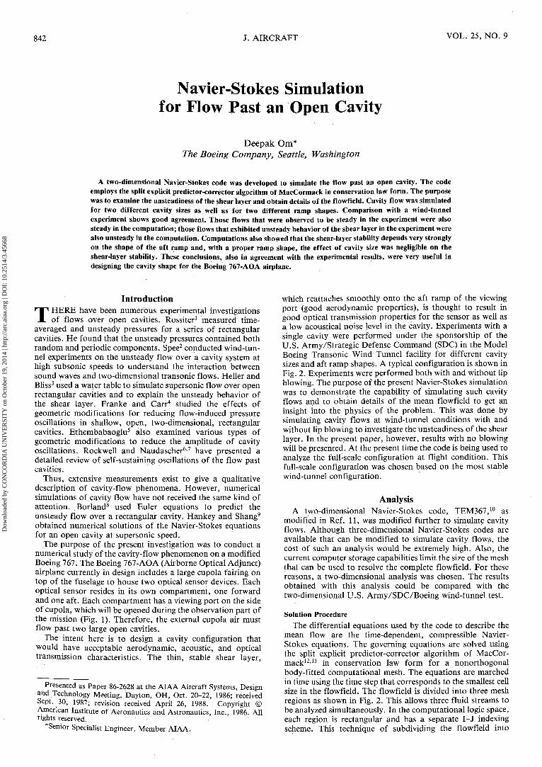
which reattaches smoothly onto the aft ramp of the viewingport (good aerodynamic properties), is thought to result ingood optical transmission properties for the sensor as well asa low acoustical noise level in the cavity. Experiments with asingle cavity were performed under the sponsorship of theU.S. Army/Strategic Defense Command (SDC) in the ModelBoeing Transonic Wind Tunnel facility for different cavitysizes and aft ramp shapes. A typical configuration is shown inFig. 2. Experiments were performed both with and without lipblowing. The purpose of the present Navier-Stokes simulationwas to demonstrate the capability of simulating such cavityflows and to obtain details of the mean flowfield to get aninsight into the physics of the problem. This was done bysimulating cavity flows at wind-tunnel conditions with andwithout lip blowing to investigate the unsteadiness of the shearlayer. In the present paper, however, results with no blowingwill be presented. At the present time the code is being used toanalyze the full-scale configuration at flight condition. Thisfull-scale configuration was chosen based on the most stablewind-tunnel configuration.

AnalysisA two-dimensional Navier-Stokes code, TEM367,10 as

modified in Ref. 11, was modified further to simulate cavityflows. Although three-dimensional Navier-Stokes codes areavailable that can be modified to simulate cavity flows, thecost of such an analysis would be extremely high. Also, thecurrent computer storage capabilities limit the size of the meshthat can be used to resolve the complete flowfield. For thesereasons, a two-dimensional analysis was chosen. The resultsobtained with this analysis could be compared with thetwo-dimensional U.S. Army/SDC/Boeing wind-tunnel test.

Solution ProcedureThe differential equations used by the code to describe the

mean flow are the time-dependent, compressible Navier-Stokes equations. The governing equations are solved usingthe split explicit predictor-corrector algorithm of MacCor-mack12'13 in conservation law form for a nonorthogonalbody-fitted computational mesh. The equations are marchedin time using the time step that corresponds to the smallest cellsize in the flowfield. The flowfield is divided into three meshregions as shown in Fig. 2. This allows three fluid streams tobe analyzed simultaneously. In the computational logic space,each region is rectangular and has a separate I-J indexingscheme. This technique of subdividing the flowfield into

Dow

nloa

ded

by C

ON

CO

RD

IA U

NIV

ER

SIT

Y o

n O

ctob

er 1

9, 2

014

| http

://ar

c.ai

aa.o

rg |

DO

I: 1

0.25

14/3

.456

68

SEPTEMBER 1988 FLOW PAST AN OPEN CAVITY 843

DOMAIN I

r~ VIEWING PORT

Fig. 1 Cupola fairing on top of 767 fuselage.

0.6 T

0.4

Y(m)

0.2

REGION III

REGION I

0.0X(m)

Fig. 2 Three regions of the flowfield.

DOMAIN II -

Y(m)

U.b-

0.4

0.2

n n -

———————————————— UUMAIN IV

DOMAIN 1 /"~~"N DOMAIN III

DOMAIN IV

-0.4 -0.2 0.0 0.2 0.4 0.6X(m)

Fig. 3 Four domains for generating grids.

0.50

Y(m)

0.300 0.10 0.20 0.30 0.40 0.50 0.60

X(m)

Fig. 4a Hyperbolic grid for domain III.

several coupled computational regions conserves computerstorage and eases mesh generation.

Grid GenerationIn the original code, the I-mesh lines were vertical and

parallel to the y -coordinate axis and the J-mesh lines werefitted to the body. The mesh system generated by this coderesulted in highly sheared meshes near the edge of the aftramp. The resultant truncation errors associated with thesemeshes caused the program to blow up in the region of shearedmeshes. For this reason, it was decided to use a hyperbolicH-mesh to reduce mesh shearing.

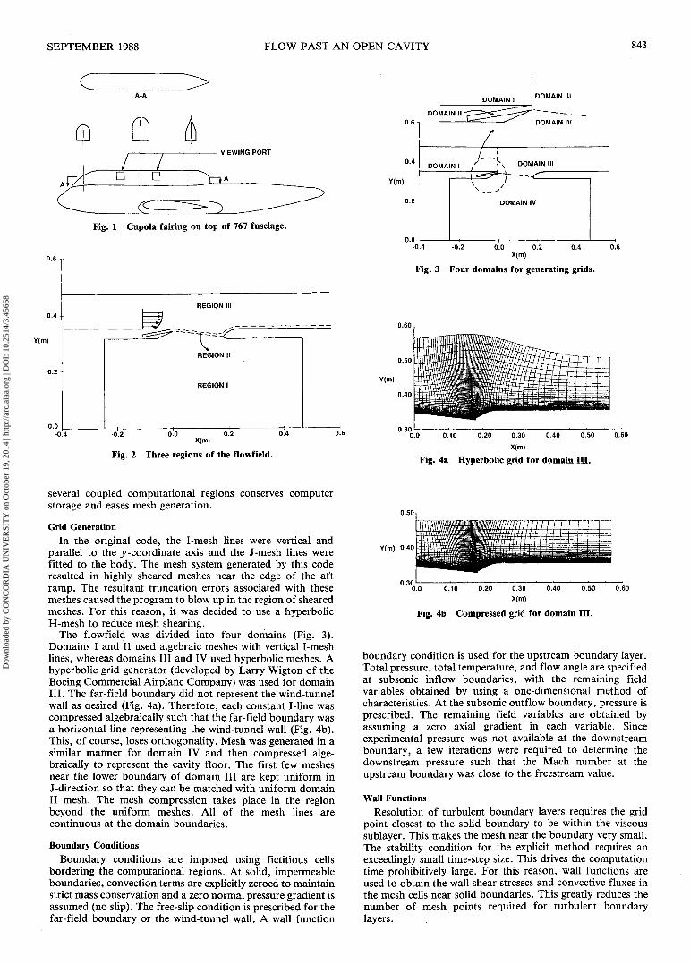
The flowfield was divided into four domains (Fig. 3).Domains I and II used algebraic meshes with vertical I-meshlines, whereas domains III and IV used hyperbolic meshes. Ahyperbolic grid generator (developed by Larry Wigton of theBoeing Commercial Airplane Company) was used for domainIII. The far-field boundary did not represent the wind-tunnelwall as desired (Fig. 4a). Therefore, each constant I-line wascompressed algebraically such that the far-field boundary wasa horizontal line representing the wind-tunnel wall (Fig. 4b).This, of course, loses orthogonality. Mesh was generated in asimilar manner for domain IV and then compressed alge-braically to represent the cavity floor. The first few meshesnear the lower boundary of domain III are kept uniform inJ-direction so that they can be matched with uniform domainII mesh. The mesh compression takes place in the regionbeyond the uniform meshes. All of the mesh lines arecontinuous at the domain boundaries.

Boundary ConditionsBoundary conditions are imposed using fictitious cells

bordering the computational regions. At solid, impermeableboundaries, convection terms are explicitly zeroed to maintainstrict mass conservation and a zero normal pressure gradient isassumed (no slip). The free-slip condition is prescribed for thefar-field boundary or the wind-tunnel wall. A wall function

Y(m) 0.40

0.300.0 0.10 0.20 0.30 0.40 0.50 0.60

X(m)

Fig. 4b Compressed grid for domain III.

boundary condition is used for the upstream boundary layer.Total pressure, total temperature, and flow angle are specifiedat subsonic inflow boundaries, with the remaining fieldvariables obtained by using a one-dimensional method ofcharacteristics. At the subsonic outflow boundary, pressure isprescribed. The remaining field variables are obtained byassuming a zero axial gradient in each variable. Sinceexperimental pressure was not available at the downstreamboundary, a few iterations were required to determine thedownstream pressure such that the Mach number at theupstream boundary was close to the freestream value.

Wall FunctionsResolution of turbulent boundary layers requires the grid

point closest to the solid boundary to be within the viscoussublayer. This makes the mesh near the boundary very small.The stability condition for the explicit method requires anexceedingly small time-step size. This drives the computationtime prohibitively large. For this reason, wall functions areused to obtain the wall shear stresses and convective fluxes inthe mesh cells near solid boundaries. This greatly reduces thenumber of mesh points required for turbulent boundarylayers.

Dow

nloa

ded

by C

ON

CO

RD

IA U

NIV

ER

SIT

Y o

n O

ctob

er 1

9, 2

014

| http

://ar

c.ai

aa.o

rg |

DO

I: 1

0.25

14/3

.456

68

844 D. OM J. AIRCRAFT

Turbulence ModelAlgebraic eddy-viscosity turbulence models used in the code

are described in detail in Ref. 10. A two-layer mixing-lengthmodel was used to describe the boundary layer. A simplemixing-length model was used to describe the shear layer inwhich the eddy viscosity is proportional to the thickness of themixing layer and the difference between the tangentialvelocities across the layer. The mixing-layer thickness wasassumed to vary linearly with downstream distance having aninitial value equal to the upstream boundary-layer thickness.

When the shear layer reattaches itself on the aft ramp, theuse of an algebraic eddy-viscosity turbulence model does notseem feasible for this complex region, where the length scaleof turbulence must make the transition from a free shear layerto an attached boundary layer. The problem is the a priorispecification of a length scale. An appropriate choice wouldbe the use of a two-equation model that calculates its ownlength scale. Since the main interest of the present study wasto study the shear-layer oscillati6n and not the redevelopmentof the boundary layer, it was decided to use the existingalgebraic turbulence model present in the code. Over the rampsurface, the eddy viscosity is computed using the boundary-layer model.

Smoothing TermsIn regions of low fluid velocity and particularly regions

where there exist large second derivatives in the conservativefield variables, the algorithm requires smoothing to preventnumerical instability. Explicit smoothers are added using thefourth-order pressure term introduced by MacCormack andBaldwin.13 In addition, a linear diffusion term was included,which was used mainly to damp large transients generated bythe initial conditions. The two smoothers are combined in asingle term and added to each of the field equations.

Initial ConditionsOutside the cavity (region III of Fig. 2), the upstream

condition is imposed everywhere. Inside the cavity (region I ofFig. 2), the flow is assumed to be static, i.e., (7 = 0, V = 0,T = TQ, and P = P^. Region II (Fig. 2) flow is also assumed tobe static.

The present code has a restart capability. The solutiongenerated for a particular mesh may be used as the initialcondition for subsequent computations involving the samemesh size but with a different CFL number or artificialviscosity coefficient.

Results and DiscussionThis paper presents results of the Navier-Stokes analysis for

three wind-tunnel cases, the data for which were made avail-able by the U.S. Army/SDC. The freestream total pressurewas 1 atm and the total temperature was 300 K. The cavityviewing port length is 0.1778 m (7.0 in.). M^ and 6, thethickness of the turbulent boundary layer, correspond to theupstream computational boundary. The three wind-tunnelcases are as follows:

I) 14 x 31 in. cavity size with a blunt ramp: M^ -0.65,6~ 1.0 in. (2.54cm).

II) 11 x 17 in. cavity size with a blunt ramp: M^ ~ 0.65,d = 1.0 in. (2.54cm).

III) 11 x 17 in. cavity size with a sharp ramp: M^ ~ 0.65,6= 1.0 in. (2.54cm).

All of the computations were performed on a Cray X-MPmachine. The number of cycles marched for each case is givenin the respective subsections that follow.

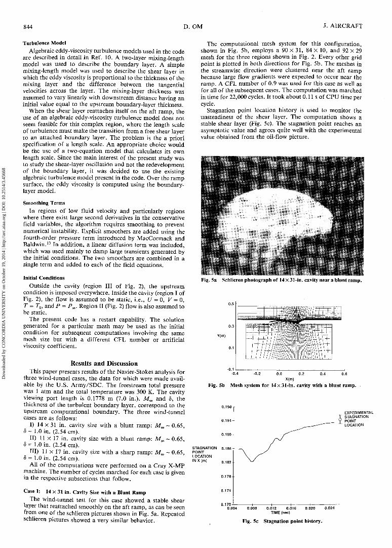
Case I: 14 x 31 in. Cavity Size with a Blunt RampThe wind-tunnel test for this case showed a stable shear

layer that reattached smoothly on the aft ramp, as can be seenfrom one of the schlieren pictures shown in Fig. 5a. Repeatedschlieren pictures showed a very similar behavior.

The computational mesh system for this configuration,shown in Fig. 5b, employs a 90 x 31, 84 x 10, and 92 x 29mesh for the three regions shown in Fig. 2. Every other gridpoint is plotted in both directions for Fig. 5b. The meshes inthe streamwise direction were clustered near the aft rampbecause large flow gradients were expected to occur near theramp. A CFL number of 0.9 was used for this case as well asfor all of the subsequent cases. The computation was marchedin time for 22,000 cycles. It took about 0.11 s of CPU time percycle.

Stagnation point location history is used to monitor theunsteadiness of the shear layer. The computation shows astable shear layer (Fig. 5c). The stagnation point reaches anasymptotic value and agrees quite well with the experimentalvalue obtained from the oil-flow picture.

Fig. 5a Schlieren photograph of 14 x 31-in. cavity near a blunt ramp.

Y(m)

-0.4 0.0 0.2 0.6X(m)

Fig. 5b Mesh system for 14 x 31-in. cavity with a blunt ramp.

STAGNATIONPOINTLOCATIONIN X (m)

EXPERIMENTALSTAGNATIONPOINTLOCATION

0.012 0.016TIME (sec)

0.020 0.024

Fig. 5c Stagnation point history.

Dow

nloa

ded

by C

ON

CO

RD

IA U

NIV

ER

SIT

Y o

n O

ctob

er 1

9, 2

014

| http

://ar

c.ai

aa.o

rg |

DO

I: 1

0.25

14/3

.456

68

SEPTEMBER 1988 FLOW PAST AN OPEN CAVITY 845

Velocity vectors at time = 20.48 ms are shown in Fig. 5d.The velocity vector plot shows a large recirculating flow nearthe aft ramp. Thus, mass is entrained into the cavity near theaft ramp, and it goes out of the cavity from the upstream endof its opening. This, in turn, causes a counterrotating flow inthe right side of the cavity. This flow is responsible forproducing the reversed flow underneath the ramp, which wasalso observed experimentally using the oil-flow technique.14

The Mach number contour at time = 20.48 ms is shown inFig. 5e. The upstream boundary layer becomes a shear layerover the cavity and reattaches itself on the aft ramp. Theproximity of the wind-tunnel wall to the cavity forms achannel over the ramp surface. The boundary layer down-stream in this channel becomes much thicker, as expected. Theother main features of the flow include the following: 1) verylow Mach number flow in the cavity, and 2) an increasedfreestream Mach number in the downstream channel. Withthe displacement thickness buildup in the downstream chan-nel, the effective area of the channel is reduced, whichproduces a higher Mach number flow.

The density contour at time = 20.48 ms is shown in Fig. 5f.It shows a steady shear layer reattaching smoothly onto the aftramp, as was seen in the schlieren photograph (Fig. 5a).

This suggests that, by properly contouring the aft rampshape, the shear layer can be made stable or the pressureoscillations in the shear layer can be reduced. Similarobservations were made by Franke and Carr4 and Ethem-babaoglu5 in their experimental investigations.

Case II: 11 x 17 in. Cavity Size with the Blunt RampThe wind-tunnel test for this case showed a stable shear

layer, as can be seen from one of the schlieren pictures shownin Fig. 6a. Repeated schlieren pictures showed a very similarbehavior.

The computational mesh system for this configuration, asshown in Fig. 6b, employs a 79 x 29, 84 x 10, and 92 x 29mesh for the three regions. The computation was marched intime for 17,000 cycles. It took about 0.1044 s of CPU time percycle. The computational results show a stable shear layer, asseen in Fig. 6c. The flow behaves very similar to the case Iflow. Experimental stagnation point location was not avail-able for this case as well as for the subsequent case. Machnumber contours at time = 19.36 ms are shown in Fig. 6d.

Case III: 11 X 17 in. Cavity Size with a Sharp RampThis case is identical to case II except the blunt ramp is

replaced with a sharp ramp. The wind-tunnel test for this caseshowed an unstable shear layer, as can be seen from one of theschlieren pictures shown in Fig. 7a. Repeated schlierenpictures showed an unsteady shear layer.

The computational mesh system for this configuration, asshown in Fig. 7b, employs 80 x 29, 84 x 10, and 92 x 29 meshfor the three regions. The computation was marched in timefor 13,000 cycles. It took about 0.16 s of CPU time per cycle.The computational results show an unsteady shear layer, ascan be seen from the stagnation point history (Fig. 7c).Stagnation point history (Fig. 7c) shows that the shear layerreattaches on the aft ramp but oscillates about a certain pointon the ramp. Pressure histories at two points in the shear layer(Figs. 7d and 7e) also show the unsteady nature of the shearlayer. The average pressure at P3R (Fig. 7d), which is near thestagnation point, is higher than the average pressure at P3L(Fig. 7e), as expected. The Mach number contour at time= 18.83 ms is shown in Fig. 7f.

A comparison of the Mach number contour (Fig. 7f) withthe Mach number contour of the same cavity size but with ablunt ramp (Fig. 6d) shows that the Mach number inside thecavity is higher for the sharp ramp. This suggests that moremass is entrained into the cavity for the sharper ramp, whichis probably responsible for inducing the shear-layer oscillationwith successive mass expulsion from the cavity and massentrainment into it.

Y(m)

-0.4 -0.3 -0.2 -0.1 0.0 0.1X(m)

0.2

Fig. 5d Velocity vectors at time = 20.48 ms.

0.34; " r ^ - r' T z " r *•

(m)

0.32

0.28

Fig. 5d (contd.)ms.

X(m)

Velocity vectors near the aft ramp at time = 20.48

Y(m)

1 0.0052 0.013 0.024 0.055 0.056 0.157 0.508 0.559 0.150 0.50A 0.55B 0.60C 0.65D 0.70E 0.72

-0.2 -0.1 0.2X(m)

Fig. 5e Mach number contours at time = 20.48 ms.

Y(m)

Fig. 5f Density contours at time = 20.48 ms.

Dow

nloa

ded

by C

ON

CO

RD

IA U

NIV

ER

SIT

Y o

n O

ctob

er 1

9, 2

014

| http

://ar

c.ai

aa.o

rg |

DO

I: 1

0.25

14/3

.456

68

846 D. OM J. AIRCRAFT

Fig. 6a Schlieren photograph of 11 x 17-in. cavity near a blunt ramp.

0.3

Y(m)

-0.1-0.4 -0.2 0.0 0.2 0.4 0 6

X(m)

Fig. 6b Mesh system for 11 x 17-in. cavity with a blunt ramp.

0.198

STAGNATION POINTLOCATION IN X(m)

0.178

0.009 0.014TIME (sec)

0.019

Fig. 7a Schlieren photograph of 11 x 17-in. cavity with a sharpramp.

0.3

Y(m)

-0.1-0.4 -0.2 0.0 0.2 0.4 0.6

X(m)

Fig. 7b Mesh system for 11X 17-in. cavity with a sharp ramp.

STAGNATION Q 186POINTLOCATIONINX(m)

Fig. 6c Stagnation point history.

0.006 0.008 0.010 0.012 0.014 0.016 0.018TIME (sec)

Fig. 7c Stagnation point history.

Y(m)

-0.2 -0.1 0.0 0.1 0.2 0.3 0.4 0.5X(m)

Fig. 6d Mach number contours at time = 19.36 ms.

This is consistent with Spec's2 observations from his wind-tunnel test. Spee mentions in his paper that periodical inflowsand outflows take place, from the outer flow into the cavityand back, associated with the lateral displacement at the aftramp, and caused by the fluctuating pressure differencebetween the inner and outer flows. This pressure difference inits turn is a consequence of the inflow and outflow. Spee alsofound visible variations of the stagnation point position on theaft ramp, which is consistent with the present numericalsolution (Fig. 7c).

An important condition for the generation of shear-layeroscillations can be described in terms of an effective feedback.Spee2 and Rockwell and Naudascher6 give a good descriptionof this mechanism. This feedback, which is essentially theupstream propagation of disturbances produced at the down-stream cavity edge, produces vorticity fluctuations near thesensitive shear-layer origin, which, in turn, provide enhanced

Dow

nloa

ded

by C

ON

CO

RD

IA U

NIV

ER

SIT

Y o

n O

ctob

er 1

9, 2

014

| http

://ar

c.ai

aa.o

rg |

DO

I: 1

0.25

14/3

.456

68

SEPTEMBER 1988 FLOW PAST AN OPEN CAVITY 847

PRESSURE ATP3R (N/m2)

74,0000.000 0.004 0.008 0,012 0.016

TIME (sec)

Fig. 7d Pressure history at point P3R.

Y(m)

0.3

Fig. 7g Density contours at time = 18.83 ms.

PRESSURE ATP3L (N/m2)

66,0000.000 0.004 0.008 0.012 0.016

TIME (sec)

Fig. 7e Pressure history at point P3L.

Y(m) 0.2

0.1

0.0

1 0.0052 0.013 0.024 0.055 0.056 0.157 0.508 0.559 0.150 0.50A 0.55B 0.60G 0.65D 0.70E 0.72

-0.2 -0.1 0.0 0.1 0.2 0.3 0.4 0.5 0.6X(m)

Fig. 7f Mach number contours at time = 18.83 ms.

disturbances to be amplified further in the shear layer, andso on.

The density contour, shown in Fig. 7g, clearly exhibits anunsteady behavior of the shear layer and qualitatively com-pares very favorably with the schlieren photograph of Fig. 7a.

Comment on Numerical SchemeThe split operators of MacGormack et al.,12'13 which

advance the solution from the n time level to the n + 1 timelevel, were not applied symmetrically in the original code.10

The scheme is second-order accurate in space, but since theoperators are not applied symmetrically, it is only first-orderaccurate in time. In the original code, only steady-state solu-tions were of interest; therefore, the lack of operator symmetrywas incorporated. However, for unsteady flows, second-orderaccuracy in time is desirable. But, since low GFL values areused with the explicit method, time accuracy is somewhatretained. It is felt that this would be adequate for the presentcavity problem since we are interested mainly in the qualitativedefinition of the shear-layer unsteadiness. However, in futureendeavors it is advisable to apply the operators symmetricallyto make the scheme second-order accurate in time.

It would be desirable to study the effect of mesh refinementin the normal direction over the aft ramp surface to see howwell it resolves the boundary layer. This is needed since thewall function boundary condition was not used on the rampsurface.

Concluding RemarksThe numerical simulation of the Airborne Optical Adjunct

(AOA) cavity flow using a two-dimensional, Navier-Stokescode showed good qualitative agreement with the U.S. Army/SDC wind-tunnel test. It also provided details of the flowfieldthat were not available from the wind-tunnel test. The analysisof two different cavity sizes (14 x 31 in. and 11 x 17 in.) witha blunt ramp showed that the shear layer remained stable forboth cases. When a sharp ramp was used in place of the bluntramp with the 11 x 17 in. cavity size, the shear layer exhibitedself-sustained oscillation. These results were in agreement withthe wind-tunnel results. Based on these results, the cavity withthe larger dimension (14 x 31 in.) and blunt ramp was chosenas the baseline configuration. A larger dimension of the cavityallows more room for the optical sensor.

Currently, the code is being used to analyze the full-scalecavity configuration for the 767-AOA airplane. This full-scaleconfiguration was chosen based on the wind-tunnel baselineconfiguration. The intent is to find out if the shear layer,which was stable at the wind-tunnel condition, would remainstable at the flight condition. Also, the density contoursobtained from the Navier-Stokes computation will be used toevaluate the optical transmission characteristics of the shearlayer at the flight condition.

AcknowledgmentsThis computational work was funded by the Boeing

Commercial Airplane Company. The author is thankful to theU.S. Army/SDC; to Dr. Mansop Hahn of Boeing Commer-cial Airplane Company for making available the experimentalresults; and to Edward Tinoco of Boeing CommercialAirplane Company for helpful discussions.

Dow

nloa

ded

by C

ON

CO

RD

IA U

NIV

ER

SIT

Y o

n O

ctob

er 1

9, 2

014

| http

://ar

c.ai

aa.o

rg |

DO

I: 1

0.25

14/3

.456

68

848 D. OM J. AIRCRAFT

References^ossiter, J. E., "Wind Tunnel Experiments on the Flow Over

Rectangular Cavities at Subsonic and Transonic Speeds," Aeronauti-cal Research Council, R&M 3428, Oct. 1964.

2Spee, B. M., "Wind-Tunnel Experiments on Unsteady CavityFlow at Subsonic Speeds," Separated Flow II, AGARD ConferenceProceedings, Rhode-Saint-Genese, Belgium, No. 4, May 1966.

3Heller, H. and Bliss, D., "Aerodynamically Induced PressureOscillations in Cavities: Physical Mechanisms and Suppresion Con-cepts," Wright-Patterson AFB, OH, Air Force Flight Dynamics Lab.,TR-74-133, Feb. 1975.

4Franke, M. E. and Carr, D. L., "Effect of Geometry on OpenCavity Flow-Induced Pressure Oscillations," AIAA Paper 75-492,March 1975.

5Ethembabaoglu, S., "On the Fluctuating Flow Characteristics inthe Vicinity of Gate Slots," Div. of Hydraulic Engineering, Univ. ofTrondheim, Norwegian Inst. of Technology, June 1973.

6Rockwell, D. and Naudascher E., "Review—Self-Sustaining Oscil-lations of Flow Past Cavities," Journal of Fluids Engineering, Vol.100, June 1978, pp. 152-165.

7Rockwell, D. and Naudascher, E., "Self-Sustained Oscillations ofImpinging Free Shear Layers," Annual Review of Fluid Mechanics,1979, pp. 67-94.

8Borland, C. J., "Numerical Prediction of the Unsteady Flowfieldin an Open Cavity," AIAA Paper 77-673, June 1977.

9Hankey, W. L. and Shang, J. S., "Analyses of Pressure Oscilla-tions in an Open Cavity," AIAA Journal, Vol. 18, Aug. 1980,pp. 892-898.

10Peery, K. M. and Forester, C. K., "Numerical Simulation ofMultistream Nozzle Flows," AIAA Journal, Vol. 18, Sept. 1980.

"Campbell, A. F. and Syberg, J., "Design Study of an ExternalCompression Supersonic Inlet Using a Finite-Difference Two-Dimen-sional Navier-Stokes Code," AIAA Paper 84-1275, June 1984.

12Hung, C. M. and MacCormack, R. W., "Numerical Solutions ofSupersonic and Hypersonic Laminar Flows Over a Two-DimensionalCompression Corner," AIAA Paper 75-2, Jan. 1975.

13MacCormack, R. W. and Baldwin, B. S., "A Numerical Methodfor Solving the Navier-Stokes Equations with Application to Shock-Boundary Layer Interactions," AIAA Paper 75-1, Jan. 1975.

14Hahn, M. M., Private communication, Oct. 1985.

Recommended Reading from the AIAAProgress in Astronautics and Aeronautics Series . . .

Numerical Methods forEngine-Airframe IntegrationS. N. B. Murthy and Gerald C. Paynter, editors

Constitutes a definitive statement on the current status and foreseeable possibilities incomputational fluid dynamics (CFD) as a tool for investigating engine-airframe integra-tion problems. Coverage includes availability of computers, status of turbulencemodeling, numerical methods for complex flows, and applicability of different levelsand types of codes to specific flow interaction of interest in integration. The authorsassess and advance the physical-mathematical basis, structure, and applicability ofcodes, thereby demonstrating the significance of CFD in the context of aircraftintegration. Particular attention has been paid to problem formulations, computerhardware, numerical methods including grid generation, and turbulence modeling forcomplex flows. Examples of flight vehicles include turboprops, military jets, civilfanjets, and airbreathing missiles.

TO ORDER: Write AIAA Order Department,370 L'Enfant Promenade, S.W., Washington, DC 20024Please include postage and handling fee of $4.50 with allorders. California and D.C. residents must add 6% salestax. All foreign orders must be prepaid.

1986 544 pp., illus. HardbackISBN 0-930403-09-6

AIAA Members $54.95Nonmembers $72.95

Order Number V-102

Dow

nloa

ded

by C

ON

CO

RD

IA U

NIV

ER

SIT

Y o

n O

ctob

er 1

9, 2

014

| http

://ar

c.ai

aa.o

rg |

DO

I: 1

0.25

14/3

.456

68